Image Generation for Efficient Neural Network Training in Autonomous Drone Racing

Abstract

Drone racing is a recreational sport in which the goal is to pass through a sequence of gates in a minimum amount of time, while avoiding collisions. In autonomous drone racing, one must accomplish this task by flying fully autonomously in an unknown environment by relying only on computer vision methods for detecting the target gates. Due to the challenges such as background objects and varying lighting conditions, traditional object detection algorithms based on colour or geometry tend to fail. Convolutional neural networks offer impressive advances in computer vision, but require an immense amount of data to learn. Collecting this data is a tedious process because the drone has to be flown manually, and the data collected can suffer from sensor failures. In this work, a semi-synthetic dataset generation method is proposed, using a combination of real background images and randomised 3D renders of the gates, to provide a limitless amount of training samples that do not suffer from those drawbacks. Using the detection results, a line-of-sight guidance algorithm is used to cross the gates. In several experimental real-time tests, the proposed framework successfully demonstrates fast and reliable detection and navigation.

I Introduction

Autonomous drone racing is an exciting case study that aims to motivate more experts to develop innovative ways of solving complex problems, which are applicable to other domains [1]. It is calling not only for breakthroughs in autonomous systems, but also for all intelligent robotic systems [2]. What makes drone racing such an interesting challenge for autonomous unmanned aerial vehicles (UAVs), is the cumulative complexity of each sub-problem to be solved [3], such as object detection [4], non-linear control [5] and path planning [6].

The rapid progress in the field of artificial intelligence brought a wider use of many novel concepts into robotics community, such as fuzzy logic [7], reinforcement learning [8] and deep learning [9]. Successively, with the recent breakthroughs in deep learning and the development of increasingly powerful computer chips, deep convolutional neural networks (CNNs) became the standard approach for computer vision applications [10]. They offer impressive performances, but require humongous quantities of data to learn a general representation of their target dataset [11]. It has been seen that collecting a dataset for drone racing can be tedious and time-consuming, and is rarely balanced enough to allow for good generalization of the knowledge [12].

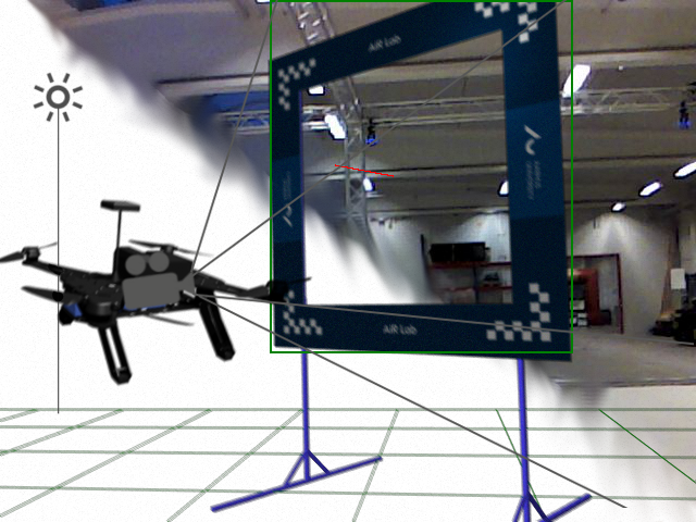
Figure 1: Semi-synthetic image generated from annotated background picture. A 3D render of a matched virtual scene is created with OpenGL, where the camera pose matches the one of the real camera used to take the background image. By using random picks from a dataset of base images annotated with their camera pose and by randomly positioning the desired meshes in the scene, an infinite amount of hybrid images can be produced.

Furthermore, available datasets do not necessarily provide adequate ground truth annotations for every application, and it can sometimes be troublesome to record a custom dataset with specific ground truth [13]. The problem also extends to deep learning in general, and large datasets of balanced data with specific ground truth labels are often hard to get hands on for unconventional applications. In the case of object detection, it might be better to create a dataset tailored to the target application domain when it differs from common challenges. This implies that a person has to spend a consequent amount of time annotating bounding boxes on each object of the dataset.

In an attempt to bypass this time-consuming process, researchers have put effort into training machine learning models directly in a simulated environment with reinforcement learning methods [14], or by feeding CNNs images extracted directly from visually realistic simulations [15]. The common conclusion to such experiments is that the model either learns too specifically about the synthetic domain [16], or benefits from a performance boost when trained on a dataset of real images enriched with synthetic ones [17].

This work proposes a novel approach to generate a semi-synthetic dataset from a combination of virtual scenes and real background images, to provide a limitless amount of racing circuit combinations to train the gate detection and distance estimation networks. The advantage of the proposed method is not limited to the generation of random and complex placement configurations, and it also provides automatic ground truth computation and annotation for virtually any measurement, as well as highly realistic scenes thanks to the alliance of real-world background photographs with modern computer graphics. The challenges of this work lie in the credibility of the generated pictures, where failure to render visually plausible scenes could cause the model to overfit on the training and validation sets. In order to assess the effectiveness of the dataset, a classical object detection CNN is trained to detect racing gates, and a convolution-based regression network is trained on the task of predicting the distance to the gate in meters.

This work is organised as follows. Section II starts with a brief overview of the related works. Section III describes the pipeline for the generation of semi-synthetic images. Section IV explains the approach to train the CNNs for the gate detection and distance estimation. Section V describes the experimental setup for real-time validation. Section VI provides offline validation of the gate detection model and the distance estimation; while Section VII presents online experimental results with a quadcopter UAV for the gate crossing, to verify the robustness of the proposed approach. Finally, Section VIII summarizes this work with conclusions and future work.

II Related Work

An early work in [18] presented a study of the use of computer graphics to render virtual scenes and images of pedestrians, and the potential adaptation for real-world usage of classifiers trained on such synthetic dataset. Even though the approach is based on engineered feature detection methods, such as histogram of gradients (HOG), and not deep convolutions, the final statement is still valid: there is a noticeable domain shift for classifiers trained on virtual-world data, only just as there would be with real-world data.

Another work, in [19], introduced a novel method for synthetic pedestrian integration on unannotated real-world background images. The novelty lies in the fact that since no annotations are used for the background dataset, an algorithm was developed to calibrate the virtual camera, compute the right pedestrians scale and infer a spawn probability map from features in the image. This method allows to overlay synthetic pedestrians onto any background image, while respecting the scale of the environment and the obstacles in the picture. Nevertheless, this approach requires a complex pipeline of algorithms to produce a visually coherent image.

To the best of the authors’ knowledge, for the specific case of autonomous drone racing, no occurrence of the use of synthetic datasets for the perception logic exists. What emerged from the literature review of the past research in this field, is that most deep learning-based methods make use of manually collected image datasets, mostly captured from a drone piloted by a human [20, 21, 22, 23]. Unfortunately, this kind of dataset is limited in the fact that it cannot be reused by other researchers without having the same test environment. The same goes for the annotations and the sensors used, which cannot be modified or enhanced without corrupting the dataset integrity. To conclude, most researchers need to create their own dataset when it comes to autonomous drone racing, simply because they have different needs in terms of the required data, and that is very time-consuming.

III Dataset Generation

With the aim of providing a way for researchers to focus on the development of their solution rather than the collection of a dataset, and to produce a theoretically infinite amount of possible configurations, a semi-synthetic dataset generation pipeline is proposed and further put to the test. The idea proposed for the aforementioned solution is to generate a virtual scene using OpenGL representing randomly positioned virtual gates that a drone would potentially have to fly through in the real world. Then, a rendered image of the scene is overlaid onto a real image, taken from the quadcopter’s camera, as to represent a random portion of a racing circuit, as seen from the UAV’s field of view. In order to do so, several requirements have to be met.

Firstly, the virtual camera must be a perfect model of the actual camera used to capture the background images, since the perspective calculation is derived from its intrinsic parameters. Therefore, the drone camera needs to be calibrated in order to estimate its intrinsic parameters, before being able to apply them to the virtual camera. Secondly, a motion capture system is used to record the position and orientation of the drone in 3D space, also known as the extrinsic parameters of the camera. This is crucial for the generation of a virtual scene whose perspective matches perfectly the perspective of the drone so that the generated scene can later be overlaid onto the real scene. Finally, the dimensions of the virtual scene must be in accordance with the actual dimensions of the physical space where the dataset of background images was recorded, otherwise unwanted artefacts such as gates being visible outside the confinement of the real scene could be produced. The same reasoning can be applied to the 3D models of gates or obstacles, since their scale matters for the usage of the generated images.

The process of generating a synthetic scene containing random meshes is done in several steps. Firstly, a virtual camera is initialized based on the real camera’s intrinsic parameters, from which a projection matrix can be derived. In a second time, a random choice of available meshes is spawned in the virtual scene, with random translations and rotations. The final step is to compute the closest gate to the camera being in its field of view, and project its center coordinates onto the image so that a ground truth label can be inferred. The general idea of this procedure is expressed as pseudo-code in Algorithm 1.

Algorithm 1 Semi-synthetic image generation

1:procedure GenerateImage

2:     $\textit{background}\leftarrow\textsc{GetRandomBaseImage}()$

3:     $\textit{cameraPose}\leftarrow\textsc{GetAnnotations}(\textit{background})$

4:     $\textit{gatePoses}\leftarrow[\,]$

5:     $i\leftarrow\textsc{Rand}(1,\textbf{MAX\_GATES})$

6:     for $i>0$ do

7:         repeat

8:              $\textit{pose}\leftarrow\textsc{RandomPose}()$

9:              $\textit{valid}\leftarrow\textbf{True}$

10:              for all gatePose in gatePoses do

11:                  $\textit{distance}\leftarrow\textsc{Norm}(\textit{pose},\textit{gatePose})$

12:                  if $\textit{distance}<\textbf{MIN\_DISTANCE}$ then

13:                       $\textit{valid}\leftarrow\textbf{False}$                                 

14:         until valid

15:         $\textit{gatePoses}[i]\leftarrow\textit{pose}$

16:         $i\leftarrow i-1$.      

17:     $\textit{scene}\leftarrow\textsc{Render}(\textit{cameraPose, gatePoses})$

18:     $\textit{scene}\leftarrow\textsc{AddNoise}(\textit{scene})$

19:     $\textit{scene}\leftarrow\textsc{AddMotionBlur}(\textit{scene})$

20:     $\textit{image}\leftarrow\textit{background}+\textit{scene}$

21:     $\textit{annotations}\leftarrow\textsc{Annotate}(gatePoses)$ return $\textit{image},\textit{annotations}$

In an OpenGL scene, the virtual camera is initialized with an up vector, an eye vector, and a target vector, as illustrated in Fig. 2. Those are passed to a helper function that computes the view matrix responsible for the 3D transformations. The target is a point in space where the camera is looking at; it is calculated by the Hamilton product of the drone orientation quaternion ($\mathbf{q}_{B}^{W}$) with the unit vector $\mathbf{\hat{x}}_{B}$ on the $\mathbf{x}_{B}$-axis (to be in front of the field of view) in the body frame, added to the drone translation, $\mathbf{r}_{W}$ in the world frame. Its final expression is as follows:

$$\mathbf{t}_{W}=\mathbf{r}_{W}+\mathbf{q}_{B}^{W}\>\mathbf{\hat{x}}_{B}\>(\mathbf{q}_{B}^{W})^{-1}.$$ (1)

As for the up vector $\mathbf{u}_{W}$, it is, in the body frame, a unit vector ($\mathbf{\hat{z}}_{B}$) orthogonal to the camera’s target vector, and calculated by the Hamilton product of the drone orientation quaternion $\mathbf{q}_{B}^{W}$ and a unit vector $\mathbf{\hat{z}}_{B}$ on the $\mathbf{z}_{B}$-axis. The final up vector in the world frame is expressed as follows:

$$\mathbf{u}_{W}=\mathbf{r}_{W}+\mathbf{q}_{B}^{W}\>\mathbf{\hat{z}}_{B}\>(\mathbf{q}_{B}^{W})^{-1}.$$ (2)

Figure 2: World frame and body frame camera coordinates. A target vector is computed from the camera extrinsics for the OpenGL camera initialization.

Once the camera is modelled and is positioned in the virtual scene, so that it matches the real world conditions, each randomly picked 3D mesh is translated and rotated in the scene. By applying random transformations, the algorithm aims to recreate unique combinations of gates for each frame. As a result, it is possible, and often the case, that only a small subset of the originally selected meshes are visible on the image frame (depending on the camera pose), or even none of them. For instance, if an extracted frame from the base dataset indicates that the drone is facing a wall up close, it would make sense not to render any gates at all to preserve coherence. In order to achieve this, the virtual scene is constrained within boundaries that match the physical environment in which the background images were recorded. The origin of the motion capture system being roughly at the centre of the premise, it is trivial to set boundaries around the origin of the virtual world, that match the ones of the physical environment.

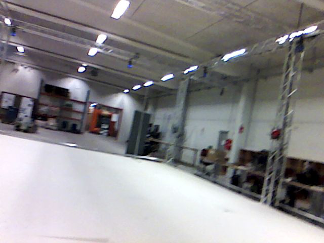
(a) Background only.

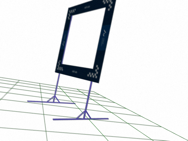
(b) Projection only.

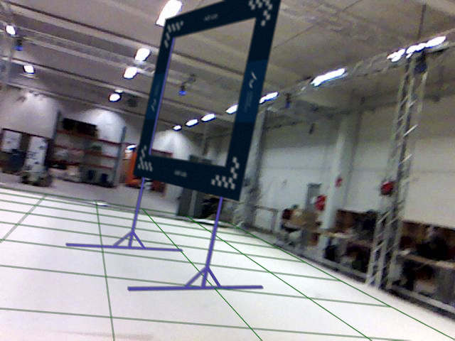
(c) Combined image.

Figure 3: The steps of a semi-synthetic image generation. Decomposition of the making of a semi-synthetic image, representing randomly positioned 3D models of randomly selected gates overlaid on top of a randomly selected real-world background image. The virtual scene’s camera is positioned and oriented using the exact configuration of the background image so that both perspectives match. The perspective grid is kept for visualization purposes.

Once the virtual scene is ready to be rendered, the annotations can be computed, namely: every gate’s bounding box coordinates and their distance to the camera. In order to compute the bounding box coordinates in the image frame, the gate centre has to be determined in the world frame, by simply applying the random 3D transformations to the centre vector parsed from a configuration file, for each mesh. From that same file, the width and height of each mesh are provided, allowing to compute easily the corners of the bounding box in the world frame. Lastly, the image frame coordinates (in pixel) can be obtained by applying the viewport transform:

$$\begin{bmatrix}x_{w}\\ y_{w}\end{bmatrix}=\begin{bmatrix}\cfrac{w}{2}x_{n}+x+\cfrac{w}{2}\\ \cfrac{h}{2}y_{n}+y+\cfrac{h}{2}\\ \end{bmatrix},$$ (3)

where $x_{w}$ and $y_{w}$ are the gate centre coordinates in the window frame (or image) and $x_{n}$ and $y_{n}$ in the normalised device coordinate system, $w$ and $h$ are the width and height of the view port – or the output image frame – and $x$ and $y$ correspond to the viewport offset in pixels, which are initially set to 0. Furthermore, to improve the correctness of the annotations and follow a human logic, an out-of-screen tolerance is added to select a target gate even if it is slightly outside of the viewport, by requiring that at least three corners of the gate be inside the frame. In that way, the intuition of targeting a gate which is clearly visible, but whose centre does not seem to be in the field of view, can be applied to the network.

The final step of forging semi-synthetic images is to merge the virtual scene into a real environment, and to blend the two images in a way that it looks as if it were real, as depicted in Fig. 3. First and foremost, a number of image deformations and distortions are applied to the rendered virtual scene. This is needed because real cameras cannot capture reality as it can be done in a controlled and sterile environment that can provide computer graphics. In particular, the camera used on the UAV produces noisy images, has a rather low resolution, does not perform well in high dynamic range and is highly subject to the motion blur. If the generated image of a still and sharp gate is simply overlaid on top of a blurry and noisy background, it will produce an incoherent and unnatural result. In order to apply a simulated motion blur, the amount of motion blur present in the background image is first estimated. This is done via the Laplacian operator, or the second order partial derivative defined as follows:

$$\nabla f=\frac{\partial^{2}f}{\partial x^{2}}+\frac{\partial^{2}f}{\partial y^{2}},$$ (4)

where $f$ is the pixel intensity. This operator detects high changes in the pixel intensity, or in other words: edges. A low amount of detected edges in the image reflects in a blurry image, where the pixel intensity is more evenly distributed. That is why the variance of the Laplacian of the image is used with a set of three thresholds, found by trial and error, to apply a different blur filter accordingly. Each of the three blur kernels has different coefficients, meaning that a different amount of synthetic motion blur is applied to the generated image by convolution, depending on the background image. Lastly, a reasonable amount of Gaussian-distributed additive noise is incorporated to the generated image. The mean value is set to $0$, while the variance is found by trial and error.

IV Convolutional Neural Networks Training

A single-shot detector is trained on the semi-synthetic dataset previously generated in Section III, and predicts bounding box coordinates for the closest visible gate. The given bounding box encloses the entire gate without its legs, as shown in Fig. 4a, and therefore the centre of this region corresponds to the desired crossing point.

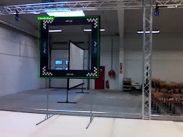
(a) Base image from the camera with bounding box annotation.

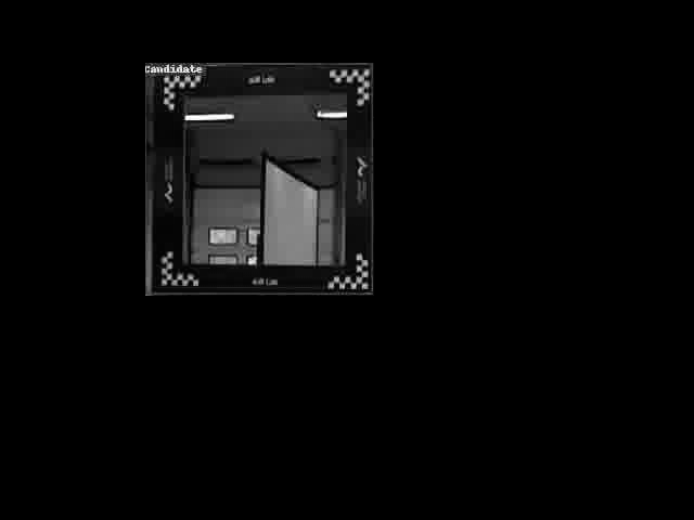
(b) Cropped image after pre-processing.

Figure 4: Region of interest extraction by cropping. The resulting image holds the essence of the distance information.

The network used for this task is the light version of SSD [24], called SSDLite, with MobileNetV2 [25] as the backbone feature extraction network. This choice is justified by the relatively low computation needs for a reasonably high detection precision. To train the network for this specific object detection task, transfer learning is used and the network architecture is left unchanged. The process only requires to change the input image resolution, the number of classes, and the different aspect ratios per layer (used for size and rotation invariance) which were set to globally match the aspect ratio of the gates at different orientations and distances to the camera.

A total of three classes were used to classify the gates: target, facing front and facing back. During training, the model’s performance is monitored using a semi-synthetic validation set, using $40\text{K}$ training samples for $4\text{K}$ validation samples. The domain shift is observed when evaluating the model on the test dataset, consisting of around $17\text{K}$ annotated images of real gates.

Furthermore, a second CNN, presented in Fig. 5, is needed to estimate the distance to the target gate. Indeed, a critical issue arises when the quadcopter gets closer to the gate: it becomes invisible in the camera’s FOV and the CNN can no longer detect it. To remedy the problem, the distance to the target gate is periodically checked during the flight, and when short enough, the crossing stage is initiated. This network is trained on a slightly different synthetic dataset consisting of grey scale images of a single gate in random orientations and distances.

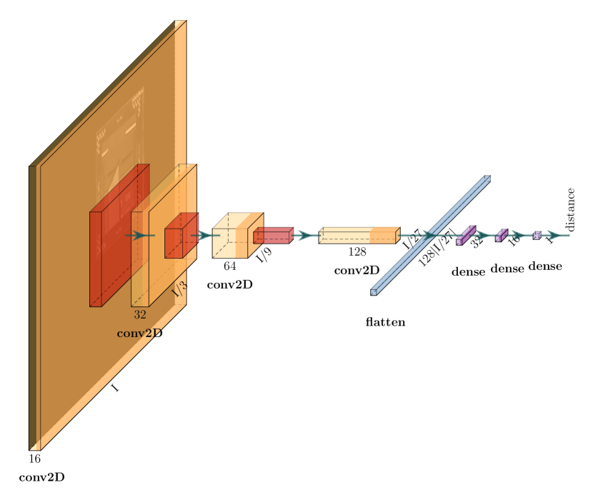
Figure 5: Topology of the proposed CNN for the estimation of the distance to the target gate. The network consists of four convolution layers with max pooling and ReLU activation functions, one flatten layer and three fully-connected layers with ReLU activation functions.

A pre-processing step is cropping the bounding box of the gate as to replace the rest of the image with black pixels, as shown in Fig. 4b. That way, only the relevant information is fed into the network, and the output is a floating-point value corresponding to the distance in meters. Finally, the perception module is implemented as a ROS node which runs the two neural networks, and does not apply any filtering to the bounding box predictions. The information published by the node contains the bounding box coordinates along with the estimated distance to the target.

V Experimental Setup

To validate the capabilities of the proposed methodology in Section VI, the Intel^® Aero Ready-to-Fly drone was chosen due to its compact size and flight characteristics that are suitable for a drone racing application. This UAV is geared for developers and researchers who desire a fast path to getting applications airborne. It is equipped with the Intel^® Aero Compute Board (CPU: Intel^® Atom^™ x7-Z8750; $4$\mathrm{G}\mathrm{B}$$ LPDDR3-1600, $32$\mathrm{G}\mathrm{B}$$ eMMC) where Linux was installed; while the robot operating system, ROS Kinetic, is used to communicate with the UAV. Moreover, the Vicon motion capture system is used to compute the UAV’s real-time velocity. The latter is fed into the extended Kalman filter (EKF) running on the Intel Aero Flight Controller with a Dronecode PX4 autopilot to obtain more accurate velocity information through sensor fusion with the data coming from inertial measurement unit. In addition, the Intel^® RealSense^™ R200 camera is used to provide an RGB video stream. This information is fed into the ground station computer (CPU (i5): $2.7$\mathrm{G}\mathrm{H}\mathrm{z}$$, $64$\mathrm{b}\mathrm{i}\mathrm{t}$$, quad-core; GPU (GeForce 940MX): $1$\mathrm{G}\mathrm{H}\mathrm{z}$$, $1$\mathrm{G}\mathrm{B}$$ GDDR5; RAM: $7$\mathrm{G}\mathrm{B}$$ DDR4) where the gate detection and distance estimation algorithms are executed. Moreover, the LeddarOne range finder is used to detect the gate crossing instant.

As for the gates to be crossed, they are made of laser-printed cardboard material glued onto a metal frame of size $1.5$\mathrm{m}$\times 1.5$\mathrm{m}$$. To provide ground truth annotations for the experiments, the motion capture system is used to record the poses of the gates and the UAV. The 3D models used for the generation of the synthetic images are $1:1$ polygon mesh representations of the actual gates.

VI Gate Detection

The performance of the gate detection model is evaluated on two datasets: a first semi-synthetic test dataset of 17K images and a test dataset consisting of 17K images of real gates. The latter was recorded with the UAV’s camera, and using the annotated 3D poses provided by the motion capture system, ground truth bounding boxes were automatically computed for the target gate only. Table I shows the average precision (AP) and average recall (AR) values for both datasets, with different intersection over union (IoU) threshold values, and for the same class representing the closest gate in the image.

TABLE I: Average precision and recall for different IoU thresholds.

IoU threshold	Semi-synthetic		Real
	AP	AR	AP	AR
0.50	0.891	0.647	0.905	0.576
0.75	0.797	0.601	0.648	0.471
0.90	0.436	0.396	0.011	0.050

A higher IoU requires the predicted bounding box to closer match the ground truth, while a lower value allows for a larger error margin. The results in Table I show an overall higher detection precision for the synthetic dataset, which is expected considering that the network was trained on such data. However, it is important to denote that the ground truth annotations for the test dataset are biased. In fact, several factors are responsible for the shift in the ground truth bounding boxes, namely: inaccurate gate 3D pose caused by manually recording it with a hand-held tracker, occluded UAV during the manual flight, network lag causing packet loss, and other possible causes. Nevertheless, an average precision of $0.9$ for an IoU of $0.5$ is a satisfying result proving that such model can be used for real time detection. Finally, Table II shows the mean average precision (mAP), AP and AR for the three classes evaluated on the synthetic test set (only the target gate ground truth could be computed for the real set). It shows that the model is well-balanced, which reflects the dataset it was trained on. This is rarely the case when manually collecting a dataset, and often leads to a biased predictor.

TABLE II: Average precision for different IoU thresholds and for every class. (synthetic dataset only)

Class	AP0.5	AP0.75	AP0.9
Target gate	0.891	0.797	0.436
Forward gate	0.819	0.726	0.231
Backward gate	0.907	0.811	0.382
mAP	0.872	0.778	0.35

Regarding the distance estimation, the model is evaluated on the same real test dataset and an equally large synthetic dataset that contains only images of single gates using the mean absolute error (MAE) in meters and an accuracy measure computed with respect to different error thresholds, as shown on Table III. One could interpret those error measurements to be high, however, precision is not required for this application, and $0.66$\mathrm{m}$$ of mean error proved to be sufficient for the crossing condition of the state machine.

TABLE III: Mean absolute error (in meters) and accuracy for different distance error thresholds.

Error threshold	Semi-synthetic		Real
(in meters)	MAE	Accuracy	MAE	Accuracy
0.75	0.401	0.854	0.660	0.660
0.50	0.401	0.722	0.660	0.505
0.25	0.401	0.445	0.660	0.283

VII Gate Crossing

The challenge of navigating through the gates is approached as a simpler sub-problem consisting of getting from point $A$ to point $B$, where $A$ is the position of the last crossed gate or starting point, and $B$ is the next gate to cross. Therefore, we opted for a state machine where each state represents a behaviour for a specific stage of the flight, since it is computationally efficient and can easily accept changes in the gate’s position. As illustrated in Fig. 6, a state machine supervises the flight and utilizes a proportional-integral-derivative (PID) controller to generate the velocity commands to align with the centre of the gate. This choice of approach is motivated by the fact that admittedly, if the nearest gate detection is quick and precise, considering a race as a succession of independent targets to be reached, it is a robust solution that can be applied to any environment with any gate of any size. For the tests, both gate detection and distance estimation networks are running off-board at $20$\mathrm{H}\mathrm{z}$$.

Figure 6: Block diagram of the proposed architecture for the real-time navigation of UAV to cross the gates.

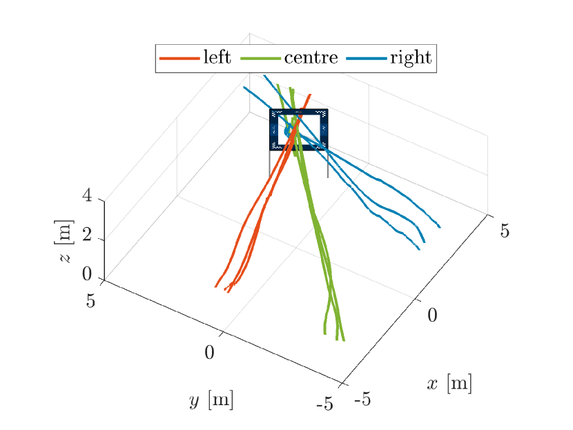
Figure 7: 3D view of the gate crossing at $2$\mathrm{m}\mathrm{/}\mathrm{s}$$ from different starting locations. It can be observed that UAV successfully crosses the gate regardless of its initial position.

To prove that the proposed method can be used in drone racing, real-time experiments are conducted, starting from three different locations (left, centre and right with respect to the gate position) for the exercise of crossing a single gate. Fig. 7 shows the 3D view of the UAV’s trajectories for different initial locations at the flying speed of $2$\mathrm{m}\mathrm{/}\mathrm{s}$$. The proposed method has not been tested for higher speeds for safety reasons, but it can be assumed by the low amount of failed attempts that the tested speed is not exploiting the full potential of the method. It is possible to observe from Fig. 7 that the proposed method is robust enough to handle fast flights and is not limited to perpendicular trajectories.

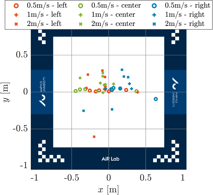
Figure 8: Gate crossing points at different speeds from different starting locations. For each speed-direction case, the experiments are repeated five times. It can be seen that at lower speed the vertical error is lower; while at higher speed the UAV tends to cross the gate in the upper part of the gate.

For the statistical analysis of navigation performances, the experiments are executed five times for three different cruise speeds ($0.5$\mathrm{m}\mathrm{/}\mathrm{s}$$, $1$\mathrm{m}\mathrm{/}\mathrm{s}$$ and $2$\mathrm{m}\mathrm{/}\mathrm{s}$$) starting from three different locations (left, centre and right) for a total of $45$ runs. A front view of the gate can be seen in Fig. 8, which shows the points at which the drone has crossed the gate. It can be observed that flights at $0.5$\mathrm{m}\mathrm{/}\mathrm{s}$$ are more stable and yield a more precise gate crossing than flights at $2$\mathrm{m}\mathrm{/}\mathrm{s}$$, where the points are more scattered and less clustered in the centre of the gate.

The Euclidean distance between the crossing point and the centre of the gate for different flying speed and starting locations is shown in Fig. 9. It is seen that on average the deviation from the centre of the gate for lower speeds ($0.5$\mathrm{m}\mathrm{/}\mathrm{s}$$ and $1$\mathrm{m}\mathrm{/}\mathrm{s}$$) has comparable magnitude; while this quantity increases for faster flights ($2$\mathrm{m}\mathrm{/}\mathrm{s}$$) because of the coupled dynamics of the UAV. Besides, the flights originating in front of the gate have predominantly lower fluctuation, since in those cases the crossing gate area is larger.

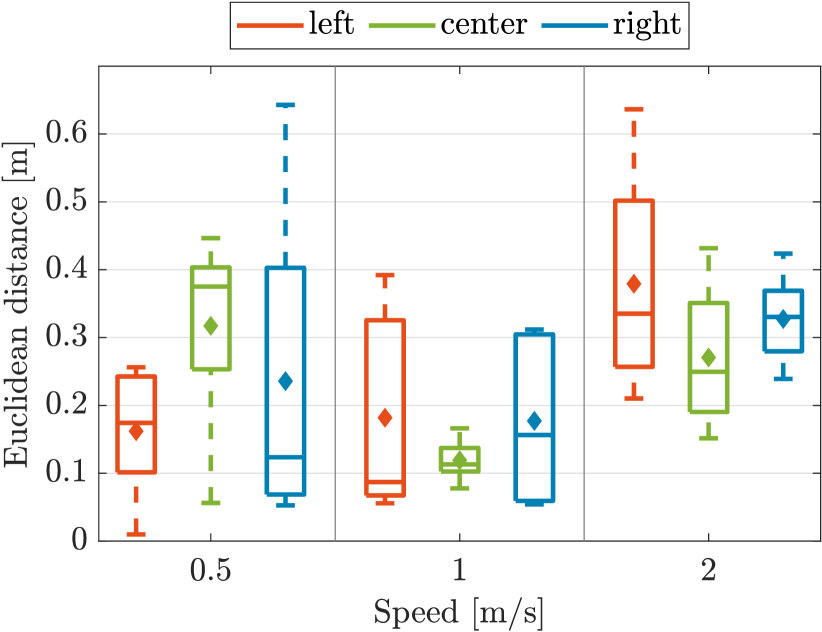
Figure 9: Euclidean distance between the crossing point and the centre of the gate at different speeds from different initial position. The diamond represents the average Euclidean distance.

VIII Conclusions and Future Work

In this work, a hypothesis on the use of synthetic images to solve the gate detection challenge in drone racing is proposed and put to the test. A complete semi-synthetic dataset generation pipeline is implemented, and this method’s results are tested on a state-of-the-art single-shot object detector. The model is evaluated on semi-synthetic images, as well as pictures of real gates. The results show that there is no significant domain shift impeding the precision of the detection. Furthermore, a flight framework is designed, based on a PID controller and a state machine. For the decision whether to cross the gate or keep aligning with it, a second, smaller CNN, is designed and trained on hybrid images to estimate the distance to the target object. The system is tested in real conditions in unknown states, and is able to successfully cross the same gate at different speeds and initial points, with a high success rate and a consistent trajectory. Thus, the proposed method for training CNNs with synthetic imagery is viable and shows to be usable for high-speed UAV flight in unknown environments, while dramatically decreasing the time spent on the preparation of a dataset.

In the future, several improvements can be brought to the proposed framework, more specifically on the control side. Adding path planning to the controller would allow for a fluid flight in a succession of gates. However, the orientation estimation of the gates must be implemented.

Supplementary Material

The real-time experimental video is available at youtu.be/T4gJgPNdiH8. The project’s code, datasets and trained models are available at: github.com/M4gicT0/autonomous-drone-racing.

References

- [1] H. Moon, J. Martinez-Carranza, T. Cieslewski, M. Faessler, D. Falanga, A. Simovic, D. Scaramuzza, S. Li, M. Ozo, C. De Wagter, G. de Croon, S. Hwang, S. Jung, H. Shim, H. Kim, M. Park, T.-C. Au, and S. J. Kim, “Challenges and implemented technologies used in autonomous drone racing,” Intelligent Service Robotics, vol. 12, no. 2, pp. 137–148, Apr 2019.
- [2] J. Delmerico, T. Cieslewski, H. Rebecq, M. Faessler, and D. Scaramuzza, “Are We Ready for Autonomous Drone Racing? The UZH-FPV Drone Racing Dataset,” in 2019 International Conference on Robotics and Automation (ICRA), May 2019, pp. 6713–6719.
- [3] S. Jung, S. Hwang, H. Shin, and D. H. Shim, “Perception, Guidance, and Navigation for Indoor Autonomous Drone Racing Using Deep Learning,” IEEE Robotics and Automation Letters, vol. 3, no. 3, pp. 2539–2544, July 2018.
- [4] C. Fu, R. Duan, D. Kircali, and E. Kayacan, “Onboard robust visual tracking for uavs using a reliable global-local object model,” Sensors, vol. 16, no. 9, p. 1406, Aug 2016.
- [5] A. Sarabakha and E. Kayacan, “Online Deep Fuzzy Learning for Control of Nonlinear Systems Using Expert Knowledge,” IEEE Transactions on Fuzzy Systems, pp. 1–1, 2019.
- [6] E. Camci and E. Kayacan, “Learning motion primitives for planning swift maneuvers of quadrotor,” Autonomous Robots, vol. 43, no. 7, pp. 1733–1745, Oct 2019.
- [7] A. Sarabakha, C. Fu, and E. Kayacan, “Intuit before Tuning: Type-1 and Type-2 Fuzzy Logic Controllers,” Applied Soft Computing, vol. 81, p. 105495, 2019.
- [8] A. Sarabakha and E. Kayacan, “Y6 Tricopter Autonomous Evacuation in an Indoor Environment using Q-Learning Algorithm,” in 2016 IEEE 55th Conference on Decision and Control (CDC), Dec 2016, pp. 5992–5997.
- [9] S. Zhou, M. K. Helwa, A. P. Schoellig, A. Sarabakha, and E. Kayacan, “Knowledge Transfer Between Robots with Similar Dynamics for High-Accuracy Impromptu Trajectory Tracking,” in 2019 18th European Control Conference (ECC), June 2019, pp. 1–8.
- [10] D. Ciregan, U. Meier, and J. Schmidhuber, “Multi-column deep neural networks for image classification,” in 2012 IEEE Conference on Computer Vision and Pattern Recognition, June 2012, pp. 3642–3649.
- [11] C. Sun, A. Shrivastava, S. Singh, and A. Gupta, “Revisiting Unreasonable Effectiveness of Data in Deep Learning Era,” in 2017 IEEE International Conference on Computer Vision (ICCV), Oct 2017, pp. 843–852.
- [12] E. Rodríguez-Hernandez, J. I. Vasquez-Gomez, and J. C. Herrera-Lozada, “Flying through Gates using a Behavioral Cloning Approach,” in 2019 International Conference on Unmanned Aircraft Systems (ICUAS), June 2019, pp. 1353–1358.
- [13] S. Jung, H. Lee, S. Hwang, and D. H. Shim, Real Time Embedded System Framework for Autonomous Drone Racing using Deep Learning Techniques.
- [14] H. X. Pham, H. M. La, D. Feil-Seifer, and L. V. Nguyen, “Autonomous UAV navigation using reinforcement learning,” CoRR, vol. abs/1801.05086, 2018.
- [15] A. Loquercio, E. Kaufmann, R. Ranftl, A. Dosovitskiy, V. Koltun, and D. Scaramuzza, “Deep drone racing: From simulation to reality with domain randomization,” CoRR, vol. abs/1905.09727, 2019.
- [16] P. Rajpura, R. Hegde, and H. Bojinov, “Object detection using deep cnns trained on synthetic images,” 06 2017.
- [17] A. Rozantsev, V. Lepetit, and P. Fua, “On rendering synthetic images for training an object detector,” Computer Vision and Image Understanding, vol. 137, pp. 24–37, Aug. 2015.
- [18] D. Vázquez, A. López, J. Marín, D. Ponsa, and D. Geronimo, “Virtual and real world adaptation for pedestrian detection,” IEEE Transactions on Pattern Analysis and Machine Intelligence, 08 2014.
- [19] E. Cheung, T. K. Wong, A. Bera, and D. Manocha, “STD-PD: generating synthetic training data for pedestrian detection in unannotated videos,” CoRR, vol. abs/1707.09100, 2017.
- [20] A. Loquercio, A. I. Maqueda, C. R. del Blanco, and D. Scaramuzza, “DroNet: Learning to fly by driving,” IEEE Robotics and Automation Letters, vol. 3, no. 2, pp. 1088–1095, Apr. 2018.
- [21] E. Kaufmann, M. Gehrig, P. Foehn, R. Ranftl, A. Dosovitskiy, V. Koltun, and D. Scaramuzza, “Beauty and the beast: Optimal methods meet learning for drone racing,” in 2019 International Conference on Robotics and Automation (ICRA). IEEE, May 2019.
- [22] E. Kaufmann, A. Loquercio, R. Ranftl, A. Dosovitskiy, V. Koltun, and D. Scaramuzza, “Deep drone racing: Learning agile flight in dynamic environments,” CoRR, vol. abs/1806.08548, 2018.
- [23] D. K. Kim and T. Chen, “Deep neural network for real-time autonomous indoor navigation,” CoRR, vol. abs/1511.04668, 2015.
- [24] W. Liu, D. Anguelov, D. Erhan, C. Szegedy, S. Reed, C.-Y. Fu, and A. C. Berg, “SSD: Single Shot MultiBox Detector,” in Computer Vision – ECCV 2016, B. Leibe, J. Matas, N. Sebe, and M. Welling, Eds. Cham: Springer International Publishing, 2016, pp. 21–37.
- [25] M. Sandler, A. Howard, M. Zhu, A. Zhmoginov, and L. Chen, “MobileNetV2: Inverted Residuals and Linear Bottlenecks,” in 2018 IEEE/CVF Conference on Computer Vision and Pattern Recognition, June 2018, pp. 4510–4520.