Dynamical Mean-Field Theory for Markovian Open Quantum Many-Body Systems

Abstract

Open quantum many body systems describe a number of experimental platforms relevant for quantum simulations, ranging from arrays of superconducting circuits hosting correlated states of light, to ultracold atoms in optical lattices in presence of controlled dissipative processes. Their theoretical understanding is hampered by the exponential scaling of their Hilbert space and by their intrinsic nonequilibrium nature, limiting the applicability of many traditional approaches. In this work we extend the nonequilibrium bosonic Dynamical Mean Field Theory (DMFT) to Markovian open quantum systems. Within DMFT, a Lindblad master equation describing a lattice of dissipative bosonic particles is mapped onto an impurity problem describing a single site embedded in its Markovian environment and coupled to a self-consistent field and to a non-Markovian bath, where the latter accounts for fluctuations beyond Gutzwiller mean-field theory due to the finite lattice connectivity.We develop non-perturbative approach to solve this bosonic impurity problem, which dresses the impurity, featuring Markovian dissipative channels, with the non-Markovian bath, in a self-consistent scheme based on a resummation of non-crossing diagrams. As a first application of our approach, we address the steady-state of a driven-dissipative Bose-Hubbard model with two-body losses and incoherent pump. We show that DMFT captures hopping-induced dissipative processes, completely missed in Gutzwiller mean-field theory, which crucially determine the properties of the normal phase, including the redistribution of steady-state populations, the suppression of local gain and the emergence of a stationary quantum-Zeno regime. We argue that these processes compete with coherent hopping to determine the phase transition towards a non-equilibrium superfluid, leading to a strong renormalization of the phase boundary at finite-connectivity. We show that this transition occurs as a finite-frequency instability, leading to an oscillating in time order parameter, that we connect with a quantum many-body synchronization transition of an array of quantum van der Pol oscillators.

I Introduction

Developments in quantum science and quantum engineering have brought forth a variety of platforms to store, control and process information at genuine quantum levels. Examples include trapped atoms and ions Cirac and Zoller (1995), quantum cavity-QED systems Raimond et al. (2001), superconducting qubitsSchoelkopf and Girvin (2008) or quantum optomechanical systems Aspelmeyer et al. (2014). These architectures are not only of great relevance for quantum technologies but also for the quantum simulation of emergent collective many-body phenomena. We now have several experimental quantum simulators worldwide running on a variety of architectures, from ultracold atoms in optical lattices Bloch et al. (2012), Rydberg gases Browaeys and Lahaye (2020), trapped ions Blatt and Roos (2012) and coupled cavity arrays Houck et al. (2012). Such simulators have led to significant advances in our understanding of quantum many-body phases and offer us an opportunity to address deep unanswered questions concerning the behavior of quantum matter in novel unexplored regimes, particularly far away from thermal equilibrium.

Many of these systems are typically characterized by excitations with a finite lifetime, due to unavoidable losses, dephasing and decoherence processes originating from their coupling to external environments and therefore feature an intrinsic nonequilibrium nature. Arrays of circuit QED cavities, for example, are emerging as a unique platform for the quantum simulation of driven-dissipative quantum many body systems Houck et al. (2012); Salathé et al. (2015); Puertas Martínez et al. (2019); Carusotto et al. (2020), where the balance of drive and loss processes and the presence of strong non-linearities, allows one to reach interesting non-equilibrium stationary states. Experiments have recently started to show a variety of dissipative quantum phases and phase transitions Fink et al. (2017); Fitzpatrick et al. (2017); Fink et al. (2018); Raftery et al. (2014), including the recent experimental realization of a dissipatively stabilised Mott insulator Ma et al. (2019). On a different front, recent advances with ultracold atoms in optical lattices allow the engineering of controlled dissipative processes, such as correlated losses Syassen et al. (2008); Tomita et al. (2017) or heating due to spontaneous emission Lüschen et al. (2017); Bouganne et al. (2020) and to study the resulting quantum many body dynamics over long time scales. These experimental settings offer fresh new inputs for quantum simulation of strongly correlated driven-dissipative quantum many-body systems, at the interface between quantum optics and condensed matter physics Carusotto and Ciuti (2013); Ritsch et al. (2013); Schmidt and Koch (2013); Hur et al. (2016); Noh and Angelakis (2017); Hartmann (2016).

From a theoretical standpoint these experimental platforms can be well described as open Markovian quantum systems, of either fermionic/bosonic particles or quantum spins, evolving through a Lindblad master equation for the many body density matrix $\rho$ Breuer and Petruccione (2007)

$$\partial_{t}\rho=-i[H,\rho]+\sum_{\alpha}\left(L_{\alpha}\rho L_{\alpha}^{\dagger}-\frac{1}{2}\left\{L^{\dagger}_{\alpha}L_{\alpha},\rho\right\}\right)\,.$$ (1)

The crucial aspect of this problem lies in the interplay between unitary dynamics and the dissipative evolution controlled by jump operators $L_{\alpha}$, out of which non trivial stationary states can be engineered Diehl et al. (2008); Verstraete et al. (2009); Murch et al. (2012); Leghtas et al. (2015). Open Markovian quantum many body systems are predicted to display a broad range of new transient dynamical phenomena Diehl et al. (2010); Poletti et al. (2012, 2013); Ludwig and Marquardt (2013) and dissipative quantum phase transitions Sieberer et al. (2013); Marino and Diehl (2016); Schiró et al. (2016); Minganti et al. (2018); Rota et al. (2019a); Young et al. (2020).

Solving the Lindblad equation for many-body systems is extremely challenging. Exact numerical solutions based on the diagonalization of the Lindbladian superoperator, or direct time evolution, are limited to very small systems, and only slightly larger systems can be addressed with quantum trajectories Daley (2014). For one dimensional systems an efficient representation of the problem in the language of matrix product operator is possible Verstraete et al. (2004); Zwolak and Vidal (2004) and has been successfully used in the recent past Kilda and Keeling (2019a), however its extension to higher dimensional systems poses problems, although some recent results have been obtained Kshetrimayum et al. (2017); Landa et al. (2020); Kilda et al. (2021). As a result, a number of theoretical approaches have been developed in recent years to tackle driven-dissipative lattice systems Finazzi et al. (2015); Weimer (2015); Jin et al. (2016); Sieberer et al. (2016); Biondi et al. (2017a); Vicentini et al. (2018); Weimer et al. (2019); Vicentini et al. (2019); Yoshioka and Hamazaki (2019); Nagy and Savona (2019); Hartmann and Carleo (2019); Landa et al. (2020). Driven-dissipative correlated bosons, such as those described by Bose-Hubbard and related models, are particularly challenging to tackle numerically due to the unbounded Hilbert space.

A powerful non-perturbative approach to quantum lattice models, based on the limit of large lattice connectivity $z$ Metzner and Vollhardt (1989); Georges and Kotliar (1992), is provided by the dynamical mean field theory (DMFT) of correlated electrons Georges et al. (1996) and bosons Byczuk and Vollhardt (2008); Anders et al. (2010, 2011). When applied to equilibrium lattice bosons DMFT captures, non-perturbatively, the $1/z$ corrections to Gutzwiller mean-field theory through the solution of a quantum impurity model. Originally introduced for equilibrium problems, DMFT has been successfully applied to a variety of nonequilibrium fermionic problems with or without dissipation Aoki et al. (2014), including Markovian fermions Panas et al. (2019), and to study unitary dynamics of correlated bosons Strand et al. (2015a).

In this work we introduce a new approach to Markovian bosonic quantum many-body systems. Specifically we extend the bosonic non-equilibrium DMFT Strand et al. (2015a) to systems evolving under the Lindblad master equation (1) and combine it with a strong coupling impurity solver tailored for correlated dissipative processes described by many-body jump operators. In the large connectivity limit DMFT maps the Lindblad dynamics (1) onto a dissipative quantum impurity model describing a single interacting bosonic mode, subject to many-body Markovian dissipation, coupled to a coherent field and a non-Markovian environment both to be determined self-consistently. The non-Markovian DMFT bath describes the effect of hopping processes from neighboring sites, which are completely missed by Gutzwiller mean-field theory. We will show that these processes are particularly interesting in open quantum systems since they not only introduce coherent effects but also provide new dissipative channels.

Solving the resulting quantum impurity model in presence of multiple many-body jump operators remains highly non-trivial and state of the art impurity solvers for non-equilibrium DMFT cannot be efficiently used in this setting. Here we build upon our recent work on Markovian impurity models Schiro and Scarlatella (2019) to develop and benchmark a DMFT solver for driven-dissipative bosonic systems. This approach is based on a super-operator hybridization expansion and resummation of an infinite class of diagrams known as non-crossing approximation (NCA).

As first application of the DMFT/NCA method we study a Bose-Hubbard model subject to two-particle losses and single particle incoherent pumping. This model is directly relevant for recent experiments with ultracold bosonic atoms in optical lattices under controlled dissipation Tomita et al. (2017); Bouganne et al. (2020) as well as for arrays of superconducting circuits Ma et al. (2019). We predict the emergence of a dissipative phase transition from a normal to a superfluid phase, where above a critical hopping or pump strength the system spontaneously develops a coherent field oscillating in time, and discuss the effect of finite-connectivity corrections to Gutzwiller mean-field. We highlight how this transition can be naturally interpreted as the onset of many body synchronization in an array of quantum Van der Pol oscillators, a phenomenon which recently attracted lots of attention Lee and Sadeghpour (2013); Lörch et al. (2016); Walter et al. (2014, 2015); Roulet and Bruder (2018a, b); Dutta and Cooper (2019); Giorgi et al. (2012); Manzano et al. (2013); Qiao et al. (2018); Sonar et al. (2018); Jaseem et al. (2020); Tindall et al. (2020). We show that DMFT allows to predict results which are qualitatively missed by Gutzwiller mean-field theory, including the redistribution of steady-state population and the suppression of gain due to hopping processes, a stationary quantum Zeno regime and a new competition between coherent and dissipative processes towards symmetry breaking. These results reflect in large quantitative corrections to the Gutzwiller mean-field phase diagram.

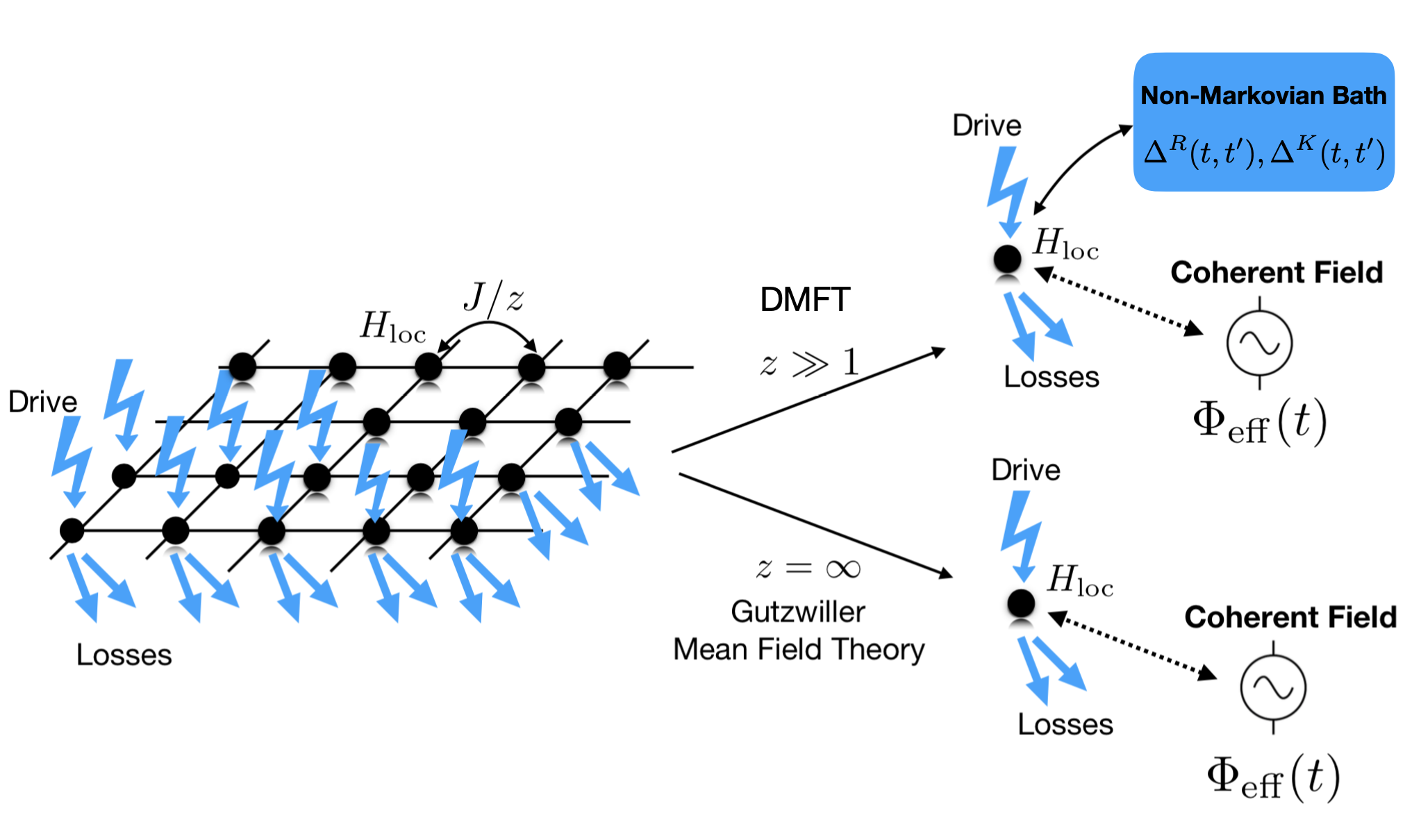
Figure 1: Sketch of the DMFT mapping for open Markovian bosonic quantum systems. A lattice of interacting, driven-dissipative bosons coupled by hopping (left, see Eq. (3-2) in the main text) is mapped in the large connectivity limit $z\gg 1$ onto a single site problem, with interactions, local Markovian drive and losses, coupled to a self-consistent environment (right, top panel). This includes a coherent drive and a non-Markovian bath (characterized by two independent hybridization functions $\Delta^{R}(t,t^{\prime})$ and $\Delta^{K}(t,t^{\prime})$) which accounts for fluctuations due to neighboring sites. In the infinite coordination limit, $z=\infty$, one recovers the Gutzwiller mean-field theory (right, bottom panel), where the effect of the lattice is simply encoded in a self-consistent field.

The paper is organized as follows. In the next section II we summarize the main concepts and results of this work, which will be presented in more detail in the rest of the paper. In Sec. III we introduce DMFT in more detail and discuss its physical content. In Sec. IV we discuss two methods to solve the quantum impurity problem: a strong coupling perturbative approach and a more powerful self-consistent NCA method. In Sec. V we present our results for an interacting Bose-Hubbard driven-dissipative lattice problem. Sec. VI is devoted to conclusions. In the Appendixes we provide technical details on the derivation of DMFT (Appendix A), a non trivial consistency check on the NCA approximation (Appendix B) and various analytical results quoted in the main text (Appendixes C-G).

II Summary of Main Results

In this section we present a summary of the main results of this work, which will be discussed more in detail in the rest of the paper. In particular in Sec. II.1 we discuss the formulation of DMFT for Markovian Bosons and of the NCA impurity solver, in Sec. II.2 we discuss our theoretical approach in relation to prior work on open quantum many-body systems, while in Sec. II.3 we present the application to a driven-dissipative Bose-Hubbard model with two-body losses and single-particle incoherent pump.

II.1 Dynamical Mean-Field Theory for Open Markovian Bosons

The class of models that we consider describe driven-dissipative bosonic particles on a lattice with coordination number $z$. The many-body density matrix of the system evolves according to a Lindblad master equation

$$\partial_{t}\rho=-i[H,\rho]+\sum_{i\mu}\left(L_{i\mu}\rho L_{i\mu}^{\dagger}-\frac{1}{2}\left\{L^{\dagger}_{i\mu}L_{i\mu},\rho\right\}\right)\,.$$ (2)

with a set of local jump operators for each lattice site $L_{i\mu}$, accounting for dissipative processes, and with coherent evolution governed by the Hamiltonian

$$H=-\frac{J}{z}\sum_{\langle ij\rangle}\left(b^{\dagger}_{i}b_{j}+\text{hc}\right)+\sum_{i}H_{loc}[b^{\dagger}_{i},b_{i}]\,.$$ (3)

Here $[b_{i},b^{\dagger}_{i}]=1$ are bosonic modes localized around the lattice site $i$, coupled together by a nearest-neighbours hopping term $J$. $H_{loc}[b^{\dagger}_{i},b_{i}]$ is a generic local Hamiltonian, which can contain arbitrary local interactions. In order for the problem to remain well defined in the limit of infinite connectivity $z\rightarrow\infty$, to which we will compare our DMFT results, we scale the hopping with a $1/z$ factor which is the correct scaling for bosons Fisher et al. (1989); Byczuk and Vollhardt (2008); Anders et al. (2010)(see also Sec. III.1 for further details).

The DMFT approach considers the master equation (2) in the limit of large, but finite, lattice connectivity $z\gg 1$. In fact, when the number of neighbors $z$ of a given lattice site is large, statistical and quantum fluctuations induced by the neighboring sites get small and can be treated in an approximate way, while the local, on-site physics is accounted for exactly. As we discuss in detail in Sec. III, in the $z\gg 1$ limit the Lindblad lattice problem formally maps onto a quantum impurity model describing an interacting Markovian single-site, characterized by the same local Hamiltonian $H_{\rm loc}$ and local jump operators $L_{i\mu}$ entering Eq. (1), coupled to a time-dependent field $\Phi_{\rm eff}(t)$ acting as a coherent drive and a non-Markovian quantum bath (Fig. 1, top panel). These take into account the effect of the neighboring sites and have to be determined self-consistently through the calculation of impurity properties. As a result of the non-equilibrium nature of the problem, the non-Markovian environment is described in terms of two independent bath hybridization functions, the retarded $\Delta^{R}(t,t^{\prime})$ and Keldysh $\Delta^{K}(t,t^{\prime})$ which in a stationary-state encode information about spectrum and occupation of the single-particle excitations. In a generic non-equilibrium condition these are independent and not related by the fluctuation-dissipation theorem.

To appreciate the physical content of DMFT it is instructive to compare it with the widely used Gutzwiller mean-field theory. As we will show in Sec. III.1 the latter coincides with the $z\rightarrow\infty$ solution of the many-body master equation and corresponds to DMFT when the non-Markovian bath is set to zero. Gutzwiller mean-field theory amounts to decouple the hopping term in the Hamiltonian (3), or equivalently assumes a product-state density matrix over different lattice sites, thus reducing the full many-body problem to a single site coupled to a self-consistent coherent field (Fig. 1, bottom panel). An obvious shortcoming of the Gutzwiller approach is that it cannot capture any coherent or dissipative processes arising from the coupling to neighboring sites, unless the system is in a broken-symmetry phase with a non-vanishing local order parameter, leading to a finite self-consistent field. The result is a particularly poor description of strongly interacting, yet incoherent, normal phases such as bosonic Mott insulators or many-body quantum Zeno phases that we discuss in this work, whose local properties within Gutzwller are completely independent on the hopping and identical to those of an isolated site. In this perspective DMFT accounts non-perturbatively, through the solution of a quantum impurity model with a non-Markovian bath $\Delta\sim 1/z$, for finite-connectivity corrections to Gutzwiller mean field theory, thus capturing fluctuations induced by the neighboring sites even in absence of an order parameter.

Although simplified with respect to the full master equation, the solution of DMFT equations and in particular of the quantum impurity problem sketched in Figure 1 still poses tremendous challenges. In particular the presence a Markovian environment containing arbitrary, possibly non-linear, jump operators, in addition to local interactions and the non-Markovian DMFT bath makes this problem hard to be solved efficiently with state of the art approaches for non-equilibrium DMFT. A major result of the present work is the development and benchmark of an impurity solver for Markovian bosonic DMFT based on the super-operator hybridization expansion formulated in Ref. Schiro and Scarlatella, 2019 and applied there to a simple non-interacting fermionic resonant level model. As we will discuss more in detail in Sec. IV.2 this approach fully captures the underlying Markovian dynamics of the impurity problem in Fig 1 and accounts for the non-Markovian bath $\Delta$ through the resummation of an infinite class of diagrams in the impurity-bath coupling known as non-crossing approximation (NCA).

As we will discuss further on in the paper, the self-consistent nature of the non-crossing approximation (NCA) we use, as opposed to bare perturbative expansions to which we will compare our results, is crucial to fully capture the non-trivial correlations associated to the DMFT bath. We give a more complete picture of the DMFT formalism, including a discussion of the basic equations and of impurity solvers in Sec. III and Sec. IV.

II.2 Relation to Prior Works

Here we wish to relate our approach with respect to previous works on nonequilibrium dissipative many-body systems. In the context of fermionic nonequilibrium DMFT, dissipation at single particle level (i.e. tunneling to external metallic leads) has been included before in several works, focusing for example on steady-state transport Joura et al. (2008); Li et al. (2015); Arrigoni et al. (2013a); Titvinidze et al. (2018); Matthies et al. (2018); Murakami and Werner (2018), Floquet driven systems Tsuji et al. (2008); Murakami et al. (2017); Qin and Hofstetter (2017) or photodoping Li and Eckstein (2021). We note that this type of dissipation is straightforward to handle within DMFT and pose no additional methodological challenges since it can be included within any impurity solver used for non-equilibrium DMFT in absence of dissipation. On the other hand many-body dissipative processes, such as those we focus here in the Lindblad context or those modeling the coupling between fermions and bosonic baths, are more challenging to handle since they induce effective interactions. Up to date these have been included in non-equilibrium DMFT studies of dissipative problems only through perturbative expansions Eckstein and Werner (2013); Golež et al. (2015); Chen et al. (2016); Bittner et al. (2018); Peronaci et al. (2020). In this respect our work goes beyond those studies in that all Markovian dissipative couplings (single and many-body) are treated on the same footing and encoded in the local Lindbladian of the impurity model, which opens up the possibilities for non-perturbative treatments of those couplings. This strategy is similar in spirit to what done for Markovian fermionic systems in Ref. Panas et al., 2019, where a discretization of the DMFT bath was used to solve the impurity problem with exact diagonalization. Here instead we use the NCA impurity solver which works directly in the thermodynamic limit of an infinite bath and does not introduce any discretization, which would be particularly severe for bosonic problems such as the one we focus here.

In the context of Markovian quantum many-body systems there have been recent methodological developments to include correlations beyond mean-field theory. Although a precise comparison with DMFT is beyond the scope of this work, it is worth to discuss some of those methods here. The Cluster Mean-Field Theory Jin et al. (2016), developed for driven-dissipative quantum spin models, is similar to DMFT in that it adds short-range correlations on top of a Gutzwiller mean-field, although this is achieved through the exact solution of a finite-size cluster, rather than through an infinite (non-interacting) bath. The Corner-Space Renormalization Method Finazzi et al. (2015) performs a diagonalization of the Lindbladian in a corner of the full Hilbert space, whose size is iteratively increased. As opposed to DMFT which works in the thermodynamic limit, this is a finite-size method, which can however produce converged results for sizes much larger than brute force methods Rota et al. (2019b). Both those approaches focus naturally on static correlations encoded in the stationary state density matrix while DMFT is constructed around the frequency-resolved Green’s functions.

II.3 Application to a Driven-Dissipative Bose Hubbard Lattice

In this work, we apply DMFT to a lattice model of driven-dissipative interacting bosons by specifying the local Hamiltonian and local jump operators entering Equations (2-3). We consider for the former

$$H_{\rm loc}=\omega_{0}b^{\dagger}_{i}b_{i}+\frac{U}{2}(b^{\dagger}_{i}b_{i})^{2}$$ (4)

i.e. a characteristic frequency $\omega_{0}$ and on-site Kerr non linearity of strength $U$ while for the latter we consider two kinds ($\mu=1,2$) of jump operators for each lattice site $i$,

$$L_{i2}=\sqrt{\eta}\,b_{i}b_{i}$$ (5)

$$L_{i1}=\sqrt{r}\sqrt{\eta}\,b_{i}^{\dagger}$$ (6)

We emphasize the correlated nature of the dissipative process encoded by $L_{i2}$ which acts only on states with multiple bosonic occupancy. This term will play a key role for our results. Interestingly this kind of loss process can be realized both with ultracold atoms Syassen et al. (2008); Tomita et al. (2017) as well with superconducting circuits Lescanne et al. (2020). The resulting lattice model, Eq. (3-6), therefore describes a driven-dissipative realisation of the Bose-Hubbard model Fisher et al. (1989) whose properties in presence of incoherent drive and dissipation has been the subject of tremendous attention recently Hartmann et al. (2006); Angelakis et al. (2007); Hartmann (2010); Diehl et al. (2010); Jin et al. (2013); Le Boité et al. (2013); Lebreuilly et al. (2017); Foss-Feig et al. (2017); Biondi et al. (2017b); Vicentini et al. (2018); Rota et al. (2019a); Scarlatella et al. (2019). The specific form of dissipation we consider in Eq. (5) is rather unexplored in a many-body context, although few results are available in the literature that we will recall briefly here.

The many body master equation (1,4-6) has a global $U(1)$ symmetry, associated with the invariance of the Liouvillian with respect to the transformation $b_{i}\rightarrow b_{i}e^{i\theta}$, and is time translational invariant (TTI). In the limit of a large number of bosons per site one expects a semiclassical description to work. The model reduces then to a discretized version of Gross-Pitaevskii equation, largely studied in the context of exciton-polariton condensation Sieberer et al. (2013), which predicts a coherent phase of bosons for any $r>0$, independently of $J/U$. This phase, which spontaneously breaks both the $U(1)$ and TTI symmetry corresponds to a nonequilibrium superfluid. In the opposite regime of uncoupled sites, $J/U=0$, the steady-state density matrix is known analytically from Refs. Dodonov and Mizrahi (1997); Dykman (1978) and describes an incoherent state: it is a statistical mixture of Fock states with $\langle{b_{i}}\rangle=0$, as might be expected given the lack of any coherent driving. How those two different phases are connected upon increasing $J/U$, in the quantum regime of few bosons per site and finite lattice connectivity, is one of the main focus of this paper.

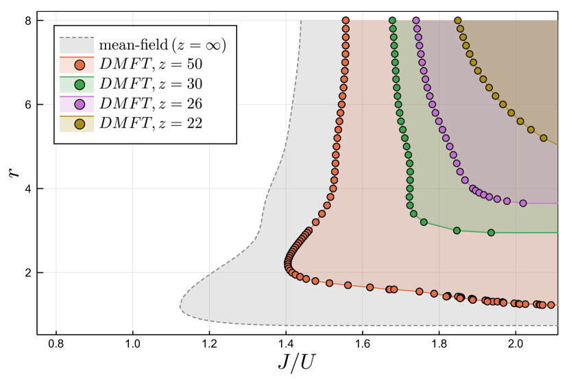
Figure 2: Phase Diagram of the Bose-Hubbard model (see Eq.(3-5)) obtained with DMFT and NCA, as a function of pump/loss ratio $r$ and hopping/interaction ratio $J/U$, for different values of the lattice connectivity $z$, compared to the Gutzwiller mean-field one ($z=\infty$). A critical line $r_{c}(J)$ separates a normal low-hopping phase from a broken symmetry phase where the system develops a local order parameter oscillating in time at finite frequency. Decreasing the lattice connectivity, i.e. increasing quantum fluctuations due to the finite number of neighbors, the ordered phase shrinks and the entire phase boundary is reshaped. In particular the re-entrant behavior of the normal phase found in mean-field disappears at small values of $z$. Parameters: $\eta/U=0.02$, $dt=0.004$, $t_{max}=10$, $dim_{H}=10$ (see Sec. V).

In Figure 2 we plot the DMFT phase diagram for our Bose-Hubbard model as a function of $r$ (the dimensionless pump-to-loss ratio) and $J/U$, for different values of the lattice connectivity $z$, together with the Gutzwiller mean field phase boundary corresponding to the $z=\infty$ limit . For a given fixed value of $z$ we find a critical line $r_{c}(J)$ separating a small-hopping normal phase where the bosons remain incoherent, $\langle b_{i}\rangle=0$, from a large hopping phase where the system develops a local order parameter breaking the $U(1)$ symmetry of the master equation. A first striking result that clearly appears from Figure 2 is that upon decreasing the connectivity, i.e. increasing the strength of fluctuations on top of the Gutzwiller mean field result, the phase diagram changes substantially. In particular the broken symmetry phase shrinks and moves toward larger values of pump and hopping. Interestingly, the DMFT corrections to the phase diagram turn out to be substantially larger than for equilibrium lattice bosons Anders et al. (2010, 2011); Strand et al. (2015a). The effect of finite-connectivity fluctuations is however not only quantitative. As we are going to discuss below, and more extensively in Sec. V, these corrections arise from a qualitatively new physics that is captured by the DMFT/NCA description of the normal phase and completely missed by Gutzwiller mean-field theory.

As we will discuss in more details in Sec. V.1-V.2, the normal phase of our model come with unique nonequilibrium properties, inherited from the local many-body physics of the single site problem Scarlatella et al. (2018). Above a pump threshold $r_{\rm ndos}$ the system develops a negative density of states (NDOS) at positive frequencies, a signature of incipient gain, i.e. energy emission in response to a weak coherent drive. Upon further increasing the pump to loss ratio above $r_{\rm inv}>r_{\rm ndos}$ the steady-state reduced density matrix shows population inversion, namely higher energy states become more occupied than lower energy ones. Within Gutzwiller mean-field theory, which describes the normal phase as a product state of single sites, those scales are independent from the hopping $J$. DMFT instead shows that fluctuations due to finite connectivity reshape completely the spectral and distribution properties of the normal phase, leading in particular to a suppression of NDoS and population inversion. This arises from hopping-induced losses, a hallmark of the interplay between coherent and dissipative dynamics in our model, which are the key physics captured by DMFT through the non-Markovian bath.

In Sec. V.3 we show that an interplay of NDoS and sufficiently strong hopping $J$ controls the true normal phase instability for values of the pump above $r_{\rm c}(J)$, when the system develops full phase coherence and enters the superfluid phase. In particular we find that the unstable mode is modulated in time and that the system displays a finite frequency phase transition corresponding to an order parameter which develops undamped oscillations, thus breaking TTI Buča et al. (2019); Iemini et al. (2018); Scarlatella et al. (2019). The large reduction of the normal phase at finite connectivity can be interpreted as an effect due to hopping-induced losses arising from the non-Markovian DMFT bath, which is able to wipe out the NDoS and absorb part of the energy emitted by the system, as we discuss more in detail in Sec. V.3.2.This mechanism for the destruction of an ordered phase is of genuine nonequilibrium origin and cannot be understood in terms of an effective heating. Indeed, as we show in Sec. V.3.3 while an effective thermalisation is captured by DMFT through an effective temperature, this remains comparable to the Gutzwiller mean-field result up to small values of the connectivity and therefore cannot explain by itself the substantial reshape of the phase diagram.

The finite-frequency transition towards an oscillating nonequilibrium superfluid shares similarities with phenomena such as lasing, limit cycles and synchronization. As we show more in detail in Sec. V.4, the driven-dissipative Bose-Hubbard (3-5) reduces in the semiclassical limit to an array of coupled classical van der Pol (vdP) oscillators Strogatz and Mirollo (1991); Matthews et al. (1991); Cross et al. (2004), which admits a stable limit cycle phase, a coherent phase with an order parameter oscillating in time at finite frequency, for any finite pump $r>0$ and any coupling $J$. In the quantum regime of few bosons per site, the picture qualitatively changes and a transition arises as a function of hopping $J$ depicted in Figure 2. This can be interpreted, in light of this analogy, as a many-body quantum synchronization Lee and Sadeghpour (2013); Lörch et al. (2016); Walter et al. (2014); Giorgi et al. (2012); Manzano et al. (2013); Walter et al. (2015); Roulet and Bruder (2018a, b); Qiao et al. (2018); Sonar et al. (2018); Davis-Tilley et al. (2018); Jaseem et al. (2020); Tindall et al. (2020); Dutta and Cooper (2019) where above a certain coupling $J$ all quantum VdP oscillators enter into a collective limit cycle phase.

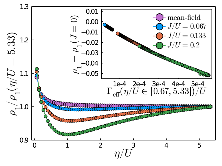
Figure 3: Emergence of Quantum Zeno Regime at fixed drive rate $f/U=r\eta/U=0.013$ and increasing two-particle loss rate $\eta$. Parameters: $t_{\rm max}=20$, $dt=0.002$, ${\rm dimH}=6$. Probability of having one boson per site in the steady-state $\rho_{1}$ as a function of $\eta/U$, rescaled by its value at $\eta/U=2.67$ for convenience. It follows a non-monotonic behaviour with a minimum at $\eta=U$, which is more pronounced the larger the hopping $J$. This behaviour is a manifestation of quantum Zeno physics, controlled by the hopping-induced loss rate $\Gamma_{\rm eff}$ as we show clearly in the inset, which is instead completely missed by Gutzwiller.

Finally, in order to highlight the role of hopping-induced dissipative processes and the qualitative differences between DMFT/NCA and Gutzwiller, in Sec. V.5 we consider the limit of large two body losses $\eta\gg J$ for our Bose-Hubbard model. We note that this regime is experimentally accessible with ultracold gases in presence of inelastic collisions Syassen et al. (2008); Tomita et al. (2017). For large two-body losses, and in absence of any external pump, perturbation theory shows that one can restrict the Bose-Hubbard dynamics to a subspace made by hard-core bosonic states, the dark states of the local dissipator García-Ripoll et al. (2009). Within this quantum Zeno subspace  Misra and Sudarshan (1977); Beige et al. (2000) the dominant dissipative processes left are those among neighboring sites, controlled by a hopping-induced loss rate $\Gamma_{\rm eff}=\frac{2(J/z)^{2}}{U^{2}+\eta^{2}}\eta$. This scale was shown to affect the transient dynamics Syassen et al. (2008); García-Ripoll et al. (2009); Rossini et al. (2020), featuring a power-law decay towards the trivial zero-density steady-state. Here we use DMFT/NCA to show that in presence of an additional small residual pump $f\ll\eta$ one can stabilize a Quantum Zeno stationary state in which physical properties are controlled by the scale $\Gamma_{\rm eff}$ (see Sec. V.5 for a detailed discussion). An example is provided in Figure 3, where we plot the DMFT/NCA steady-state occupation probability of the $n=1$ bosonic state versus $\eta/U$, for different values of $J/U$ and compare it with Gutzwiller results. The latter shows, independently of $J$, a very weak dependence from $\eta$ which would be completely absent if not for the small residual pump. DMFT results instead show a clear non-monotonous behavior as $J/U$ increases, with a minimum at $\eta\sim U$. This is a signature of the emergence of the Zeno scale $\Gamma_{\rm eff}$ controlling the physics, as we clearly reveal in the inset, where a scaling collapse is shown. We emphasize that the emergence of a Quantum Zeno stationary state represents a stringent test for the ability of DMFT of capturing hopping-induced losses, which are instead completely missed by Gutzwiller mean-field theory.

We give a more complete picture of our results for the Bose-Hubbard model in Sec. V.

III Dynamical Mean-Field Theory For Markovian Bosons

In this section we present the formalism of DMFT for Markovian bosons, including the basic self-consistency equations, its formal relation with Gutzwiller mean field theory and its physical interpretation, leaving its derivation to Appendix A. The starting point is to cast the Lindblad master equation (2) in the language of non-equilibrium Keldysh field theory, as discussed extensively in the literature Sieberer et al. (2016). The result is an action written in terms of bosonic coherent fields $\bar{b}_{i\alpha},b_{i\alpha}$ on each lattice site $i$ and on the upper/lower Keldysh contours, $\alpha=\pm$, which takes the form

$$\mathcal{S}=\int_{-\infty}^{\infty}dt\sum_{i\alpha}\alpha\bar{b}_{i\alpha}\,i\partial_{t}b_{i\alpha}-\int_{-\infty}^{\infty}dt\,i\mathcal{L}$$ (7)

where the Lindbladian $\mathcal{L}$ is given by

$$\begin{split}\mathcal{L}&=-i\left(H_{+}-H_{-}\right)+\\ &+\sum_{\mu,i}\gamma_{\mu}\left(L_{i\,\mu+}\bar{L}_{i\,\mu-}-\frac{1}{2}\bar{L}_{i\,\mu+}L_{i\,\mu+}-\frac{1}{2}L_{i\,\mu-}\bar{L}_{i\,\mu-}\right)\end{split}$$ (8)

with $H_{\alpha},L_{i\mu\alpha}$ are the expectation values of the Hamiltonian (3) and of the jump operators (5), expressed in terms of creation and annihilation operators belonging to the $\alpha$ contour, taken on bosonic coherent states. The full solution of the Keldysh action in Eq.(7) is of course not possible in general, due to the coupling between many interacting modes and the presence of interaction, drive and dissipation.

The key idea of DMFT is to write down an effective Keldysh action for the boson field of a single site of the lattice, obtained after integrating out all its neighbors Strand et al. (2015a). As we show in Appendix A, in the limit of large lattice connectivity, $z\gg 1$, this effective action has the closed form

$$\begin{split}\mathcal{S}_{\text{eff}}&[\mathbb{b}^{\dagger}_{\alpha},\mathbb{b}_{\alpha}]=S_{loc}[\mathbb{b}_{\alpha}^{\dagger},\mathbb{b}_{\alpha}]+\int dt\sum_{\alpha=\pm}\alpha\;\mathbb{\Phi}_{\text{eff}\,\alpha}^{\dagger}(t)\mathbb{b}_{\alpha}(t)+\\ &-\frac{1}{2}\int dtdt\sum_{\alpha,\beta=\pm}\alpha\beta\,\mathbb{b}^{\dagger}_{\alpha}(t)\mathbb{\Delta}^{\alpha\beta}(t,t^{\prime})\mathbb{b}_{\beta}(t^{\prime})\end{split}$$ (9)

where $\alpha,\beta$ are Keldysh contour indices and we have dropped the site index from the local boson field for simplicity (we assume translational invariance) and grouped together creation/annihilation fields into a Nambu field

$$\mathbb{b}^{\dagger}_{\alpha}=\left(\begin{array}[]{l}\bar{b}_{\alpha}\;b_{\alpha}\end{array}\right)\,\;\;\mathbb{b}_{\alpha}=\left(\begin{array}[]{l}b_{\alpha}\\ \bar{b}_{\alpha}\end{array}\right)$$ (13)

The above local Keldysh action describes a driven-dissipative quantum impurity model  Schiro and Scarlatella (2019). The first term in Eq. (9), $S_{loc}[\mathbb{b}_{\alpha}^{\dagger},\mathbb{b}_{\alpha}]$ is the local, on-site, contribution of the original lattice action (7-8) and therefore includes interactions, as well as Markovian incoherent drive and dissipation leading to off-diagonal terms in Keldysh space. The second and third terms describe the feedback of the rest of lattice onto the site through its neighbors, in terms of an effective coherent drive $\mathbb{\Phi}_{\text{eff}\,\alpha}^{\dagger}(t)$ and an effective non-Markovian bath with hybridization function $\mathbb{\Delta}^{\alpha\beta}(t,t^{\prime})$. Both these quantities have to be determined self-consistently, in particular the effective coherent drive reads

$$\mathbb{\Phi}_{\text{eff}\,\alpha}^{\dagger}=J\mathbb{\Phi}^{\dagger}_{\alpha}(t)+\int dt\,^{\prime}\sum_{\beta=\pm}\beta\mathbb{\Phi}_{\beta}^{\dagger}(t^{\prime})\mathbb{\Delta}^{\beta\alpha}(t^{\prime},t)$$ (14)

and has two contributions, the first coming from the average of the bosonic field as in Gutzwiller mean field theory

$$\mathbb{\Phi}^{\dagger}_{\alpha}=\langle{\mathbb{b}_{\alpha}^{\dagger}}\rangle_{S_{\text{eff}}}$$ (15)

and the second one coming from the non-Markovian bath, a non-trivial finite $z$ correction accounting for the feedback of neighboring sites on the local effective field Anders et al. (2010, 2011); Strand et al. (2015a). This latter term, whose origin will be discussed more in detail in Appendix A, plays a key role within DMFT, in particular for what concerns the corrections to phase diagram as we discuss in Sec. V.3-V.3.2.

The self-consistency relation for the Green’s function depends on the specific choice of the lattice. In the following we will use the simplified relation for the Bethe lattice Strand et al. (2015a)

$$\mathbb{\Delta}^{\alpha\beta}(t,t^{\prime})=\frac{J^{2}}{z}\,\mathbb{G}^{\alpha\beta}(t,t^{\prime})$$ (16)

which directly relates the hybridization function of the non-Markovian bath to the impurity connected Green’s function

$$\mathbb{G}^{\alpha\beta}(t,t^{\prime})=-i\langle\mathbb{b}_{\alpha}(t)\mathbb{b}^{\dagger}_{\beta}(t^{\prime})\rangle_{S_{\text{eff}}}+i\mathbb{\Phi}_{\alpha}(t)\mathbb{\Phi}_{\beta}^{\dagger}(t^{\prime})$$ (17)

The DMFT solution of the original Markovian lattice problem thus requires one to solve the Keldysh action (9), computing in particular the impurity Green’s function (17) and the average of the bosonic field (15), for given values of the non-Markovian bath $\Delta$ and effective field $\Phi$, and to iterate (14-16) until self-consistency.

III.1 Limit of infinite coordination number: Gutzwiller Mean Field Theory

It is instructive at this point to take explicitly the limit of infinite coordination number $z\rightarrow\infty$. In this limit, the DMFT effective action (18) becomes completely local in time

$$\begin{split}\mathcal{S}_{\text{eff}}&[\mathbb{b}^{\dagger}_{\alpha},\mathbb{b}_{\alpha}]\xrightarrow{z=\infty}S_{loc}[\mathbb{b}_{\alpha}^{\dagger},\mathbb{b}_{\alpha}]+\int\sum_{\alpha}\alpha dt\mathbb{\Phi}_{\text{eff}\alpha}^{\dagger}(t)\mathbb{b}_{\alpha}(t)\end{split}$$ (18)

since the non-Markovian bath scales as $1/z$ (See Eq.  16), and as such can be unfolded back into a master equation for a single-site density matrix $\rho$, which satisfies

$$\partial_{t}\rho(t)=i[\mathbb{b}^{\dagger}\mathbb{\Phi}(t),\rho]+\mathcal{L}\rho(t)$$

where $\mathcal{L}$ is the local part of the Lindbladian and the feedback from the neighboring sites is carried by $\mathbb{\Phi}(t)=\text{tr}[\mathbb{b}\rho(t)]$. This corresponds to a factorized Gutzwiller-like ansatz for the lattice many body density matrix

$$\rho_{\text{latt}}(t)=\prod_{i}\rho_{i}(t),$$

where $i$ is the site index and $\rho_{i}(t)\equiv\rho(t)$ because of translational invariance. In other words we have explicitly shown that, as for equilibrium or closed systems Anders et al. (2010); Strand et al. (2015a) also for driven-dissipative lattice systems the infinite connectivity limit of bosons coincides with Gutzwiller mean-field theory. We note that when $\mathbb{\Phi}=0$, this mean-field describes completely uncoupled sites, while DMFT ($z<\infty$) captures the feedback from neighboring sites through the self-consistent bath $\mathbb{\Delta}$. In the following section we are going to add some physical intuition on how the DMFT action (9) describes the effect of neighboring sites through a fictitious non-Markovian bath.

III.2 DMFT Effective Action in the Classical/Quantum basis

We now give a physical interpretation to the various terms entering the DMFT effective action in Eq. (9), in particular to the non-Markovian term. It is useful to introduce the so called classical and quantum components of the bosonic field

$$\mathbb{b}_{\rm cl/q}(t)=\frac{\mathbb{b}_{+}\pm\mathbb{b}_{-}}{\sqrt{2}}$$ (19)

$$\mathbb{b}^{\dagger}_{\rm cl/q}(t)=\frac{\mathbb{b}^{\dagger}_{+}\pm\mathbb{b}^{\dagger}_{-}}{\sqrt{2}}$$ (20)

in terms of which we can re-write the Keldysh action as

$$\begin{split}\mathcal{S}_{\text{eff}}&=S_{loc}[\mathbb{b}_{\rm cl/q}^{\dagger},\mathbb{b}_{\rm cl/q}]+\int dt\mathbb{\Phi}_{\text{eff}\,\rm cl}^{\dagger}\mathbb{b}_{\rm q}+\\ &-\frac{1}{2}\int dtdt^{\prime}\left(\mathbb{b}^{\dagger}_{\rm q}(t)\mathbb{\Delta}^{R}(t,t^{\prime})\mathbb{b}_{\rm cl}(t^{\prime})+hc\right)+\\ &-\frac{1}{2}\int dtdt^{\prime}\mathbb{b}^{\dagger}_{\rm q}(t)\mathbb{\Delta}^{K}(t,t^{\prime})\mathbb{b}^{\dagger}_{\rm q}(t^{\prime})\end{split}$$ (21)

In this basis only two independent combinations of the non-Markovian kernels $\mathbb{\Delta}^{\alpha\beta}$ enter, namely the retarded component $\mathbb{\Delta}^{R}(t,t^{\prime})=\theta(t-t^{\prime})\left(\mathbb{\Delta}^{-+}(t,t^{\prime})-\mathbb{\Delta}^{+-}(t,t^{\prime})\right)$, which couples the classical and quantum components of the field and encodes the spectral properties of the bath resulting in a frequency dependent damping for the bosonic mode and the Keldysh component $\mathbb{\Delta}^{K}=\mathbb{\Delta}^{-+}(t,t^{\prime})+\mathbb{\Delta}^{+-}(t,t^{\prime})$, encoding the occupation of the bath and resulting in a frequency dependent noise for the bosonic mode. It is worth stressing that the above Keldysh action contains quadratic, non-Markovian terms in the classical/quantum fields as well as non-linearities and higher powers of the classical/quantum fields included in the local part of the action $S_{loc}[\mathbb{b}_{\rm cl/q}^{\dagger},\mathbb{b}_{\rm cl/q}]$. While the structure of Eq. (21) is a generic feature of DMFT, the local part of the action depends on the particular form of local interaction and jump operators.

Finally, we can express also the impurity Green’s functions Eq (17) in this basis to obtain the retarded Green’s function and the Keldysh one

$$\mathbb{G}^{R}(t,t^{\prime})=-i\langle\mathbb{b}_{\rm cl}(t)\mathbb{b}^{\dagger}_{\rm q}(t^{\prime})\rangle_{S_{\text{eff}}}+i\mathbb{\Phi}_{\rm cl}(t)\mathbb{\Phi}_{\rm q}^{\dagger}(t^{\prime})$$ (22)

$$\mathbb{G}^{K}(t,t^{\prime})=-i\langle\mathbb{b}_{\rm cl}(t)\mathbb{b}^{\dagger}_{\rm cl}(t^{\prime})\rangle_{S_{\text{eff}}}+i\mathbb{\Phi}_{\rm cl}(t)\mathbb{\Phi}_{\rm cl}^{\dagger}(t^{\prime})$$

Those correlation functions contain crucial physical information about the local physics of the driven-dissipative lattice problem. The retarded Green’s function in particular encodes information about the local excitation spectrum of the system and it is known to be a crucial probe for the transition from delocalization to Mottness in strongly correlated systems at equilibrium Georges et al. (1996). For open Markovian quantum systems the retarded Green’s function contains, much like for closed equilibrium systems, information on the structure of the excitations on top of the stationary state Scarlatella et al. (2018) and it directly probes dissipative phase transitions where those excitations become unstable. Its poles correspond to eigenvalues of the Lindbladian in the single particle sector, which come with a characteristic frequency and lifetime, and their (possibly complex) weight. The retarded Green’s function has also a directly physical meaning: it describes the linear response of the expectation $\langle{b(t)}\rangle$ to a weak, classical field $h(t^{\prime})$, which couples linearly to $b^{\dagger}$. In the case where $b$ describes a photonic cavity mode, $G^{R}(t)$ can be directly measured by weakly coupling the cavity to an input-output waveguide and measuring the reflection of a weak probe tone (see e.g. Lemonde et al. (2013); Levitan et al. (2016)).

The Keldysh Green’s function on the other hand contains information about how the finite frequency excitations above the stationary state are populated. In thermal equilibrium those two functions are not independent, but constrained to satisfy the fluctuation-dissipation theorem Kamenev (2011).

III.3 Computing Lattice Quantities

Solving the DMFT effective action and computing the impurity Green’s functions (22) gives direct information on the local properties of the driven-dissipative lattice problem. Furthermore one can access non-local quantities, such as momentum distribution or non local correlation functions, through the lattice Green’s functions at momentum k

$$\mathbb{G}^{\alpha\beta}_{\textbf{k}}(t,t^{\prime})=-i\langle\mathbb{b}_{\textbf{k}\alpha}(t)\mathbb{b}^{\dagger}_{\textbf{k}\beta}(t^{\prime})\rangle+i\mathbb{\Phi}_{\textbf{k}\alpha}(t)\mathbb{\Phi}_{\textbf{k}\beta}^{\dagger}(t^{\prime})\,.$$ (23)

These satisfies a Dyson equation with a lattice self-energy $\mathbb{\Sigma}^{\alpha\beta}(t,t^{\prime})$, that within DMFT is momentum independent Georges and Kotliar (1992); Aoki et al. (2014),

$$\mathbb{G}^{\alpha\beta}_{\textbf{k}}(t,t^{\prime})=\mathbb{g}^{\alpha\beta}_{\textbf{k}}(t,t^{\prime})+\sum_{\gamma\delta}\mathbb{g}^{\alpha\gamma}_{\textbf{k}}\otimes\mathbb{\Sigma}^{\gamma\delta}\otimes\mathbb{G}^{\delta\beta}_{\textbf{k}}(t,t^{\prime})$$ (24)

and coincides with the self-energy of the impurity problem

$$\mathbb{G}^{\alpha\beta}(t,t^{\prime})=\mathbb{g}^{\alpha\beta}(t,t^{\prime})+\sum_{\gamma\delta}\mathbb{g}^{\alpha\gamma}\otimes\mathbb{\Sigma}^{\gamma\delta}\otimes\mathbb{G}^{\delta\beta}(t,t^{\prime})$$ (25)

where in the above equations $\otimes$ indicates time convolutions, $\mathbb{g}^{\alpha\beta}(t,t^{\prime})$ are the Green’s functions of the quantum impurity problem with no interactions, but including the non-Markovian bath $\mathbb{\Delta}$ and $\mathbb{g}^{\alpha\beta}_{\textbf{k}}(t,t^{\prime})$ are the non-interacting lattice Green’s functions.

IV Quantum Impurity Solvers

The main challenge behind our DMFT approach is to solve the Markovian quantum impurity model described by the Keldysh action  (9), computing in particular the Green’s functions. We stress that this remains a difficult task due to the presence of interactions on the impurity site, non-linear jump operators (such as our two-body losses) and the non-Markovian DMFT bath. While several impurity solvers have been developed in recent years for non-equilibrium DMFT Aoki et al. (2014), none of them can be efficiently applied in our case (See Sec. II.2 for a detailed discussion). To make progress we take explicit advantage of the Markovian structure of the impurity, which allows to treat non-linear jump operators as dissipative couplings of a local Lindbladian. This unleashes the possibility of developing strong-coupling impurity solvers for bosonic Markovian problems, which treat exactly the local Lindblad problem and include the effect of the non-Markovian DMFT bath through perturbative or non-perturbative schemes. We note that for non-equilibrium closed systems these strong-coupling methods represent the current state of the art of DMFT impurity solvers Aoki et al. (2014). Here we develop two such schemes for bosonic Markovian systems, the Hubbard-I approximation and the more powerful Non-Crossing-Approximation, that we both present below. We comment in the Sec. VI on possible methodological extensions.

IV.1 Hubbard-I Approximation

The simplest approximation to solve the impurity problem (9) is based on perturbation theory in the non-Markovian bath kernel $\mathbb{\Delta}$, and its lowest order is known as the Hubbard-I approximation Georges et al. (1996); Strand et al. (2015b). As we will see this approach already gives a hopping dependence of correlation functions which goes beyond Gutzwiller mean-field theory, but misses important correlations due to the non-Markovian bath. Our DMFT approach will be based on the more powerful non-crossing approximation solver which we will introduce in the next section, but we will use Hubbard-I results for comparison and to motivate the need of a more powerful solver.

For simplicity, we formulate Hubbard-I in the normal phase, where $\mathbb{\Phi}=0$ and anomalous correlation functions vanish, thus we can restrict to the first Nambu component and refer to it with non-bold symbols, e.g. $G^{\alpha\beta}=\mathbb{G}^{\alpha\beta}_{11}$ where $\alpha,\beta=\pm$ are Keldysh indexes. We also focus on the stationary state regime, where Green’s functions depend on time differences and we can move to the frequency domain i.e. $G^{\alpha\beta}(\omega)$, which is the case we will consider in our application in Sec. V.

The impurity Green’s function obeys a Dyson equation, see Eq. (25), in terms of a self-energy $\Sigma^{\alpha\beta}(\omega)$ which contains the effect of interaction, incoherent drive and dissipation and which is in general a functional of the non-Markovian bath kernel $\Delta^{\alpha\beta}(\omega)$. Hubbard-I consists in approximating the impurity self-energy by its value for ${\Delta}=0$, i.e. in absence of the bath, when it can be written as

$$\Sigma^{\alpha\beta}(\omega)\approx\left[g^{\alpha\beta}_{0}(\omega)\right]^{-1}-\left[G_{0}^{\alpha\beta}(\omega)\right]^{-1}\,.$$ (26)

Here $G^{\alpha\beta}_{0}(\omega)$ is the Green’s function of the impurity site with interaction, incoherent drive and dissipation, but without the bath (the latter condition is indicated by the index $0$); it can be computed numerically Scarlatella et al. (2018). In contrast $g^{\alpha\beta}_{0}(\omega)$ corresponds to the Green’s function of the impurity site in absence of the bath and without interactions (lowercase letter), which is known analytically. Plugging this self-energy back in the Dyson equation (25), and using the self-consistency condition on the Bethe Lattice, we obtain a closed matrix equation for the Keldysh components of the local lattice Green’s functions

$$\left[G^{\alpha\beta}(\omega)\right]^{-1}=\left[G_{0}^{\alpha\beta}(\omega)\right]^{-1}-\frac{J^{2}}{z}G^{\alpha\beta}(\omega)$$ (27)

The expressions of the retarded and Keldysh components are given explicitly in appendix E. In the appendix, we also show that the Hubbard-I approximation, despite introducing a beyond mean-field hopping dependence of Green’s functions, still yields the same phase diagram as mean-field, motivating the need for a more powerful solver.

IV.2 Super-Operator Hybridization Expansion and Non-Crossing Approximation

To go beyond the Hubbard-I approximation, we build upon the method recently formulated in Ref. Schiro and Scarlatella (2019) and applied so far only to a simple toy model fermionic system, to develop a DMFT/NCA impurity solver for bosonic Markovian systems. The idea is to perform a diagrammatic expansion in powers of the non-Markovian bath $\mathbb{\Delta}$ and to resum an infinite set of diagrams by solving a self-consistent Dyson-type equation. We remark that this expansion is carried out around an interacting problem, the single-site Markovian impurity, hence it is not based on Wick’s theorem as in weak-coupling perturbation theories. As such, working directly with Green’s functions is not convenient and the more natural formulation is in terms of evolution super-operators, that we will denote in the following with a hat Schiro and Scarlatella (2019). We start by defining the evolution super-operator $\hat{\mathcal{V}}$ of the reduced density matrix of the impurity

$$\rho_{\rm imp}(t)=\hat{\mathcal{V}}(t,0)\rho_{\rm imp}(0)$$ (28)

formally obtained by tracing out the bath degrees of freedom. We note that Eq. (28) assumes that at time $t=0$ the non-Markovian bath is not entangled with the impurity site, i.e. in the original lattice problem the initial condition corresponds to the limit of decoupled sites. Since the bath degrees of freedom are treated as non-interacting, only the single-particle Green’s function of the bath enters the reduced dynamics, the hybridization function $\mathbb{\Delta}$ introduced in Eq. (9). Expanding the super-operator $\hat{\mathcal{V}}(t,0)$ in powers of $\mathbb{\Delta}$ we obtain a series which can be represented diagrammatically as shown in Fig. 4, where bold solid lines describe the propagator $\hat{\mathcal{V}}(t,0)$, dashed lines represent the hybridization function $\mathbb{\Delta}$ while simple solid lines represent the bare Markovian evolution super-operator $\hat{\mathcal{V}}_{0}(t,0)=T\exp\left(\int_{0}^{t}dt^{\prime}\hat{\mathcal{L}}_{\text{eff}}(t^{\prime})\right)$, where $T$ is the time-ordering and $\hat{\mathcal{L}}_{\text{eff}}(t)=\hat{\mathcal{L}}_{0}+i[\hat{\mathbb{b}}^{\dagger}\hat{\mathbb{\Phi}}(t),\bullet]$ the effective single site Lindblad super-operator with argument $\bullet$.

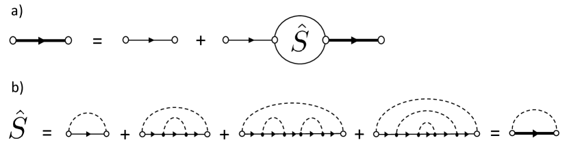
Figure 4: a) Diagrammatic representation of the Dyson series in Eq. (29). The bold (thin) solid lines represent the full, non-Markovian (bare, Markovian) impurity super-operator $\hat{\mathcal{V}}$ ($\hat{\mathcal{V}}_{0}$), while the dashed lines correspond to the non-Markovian bath $\mathbb{\Delta}$. b) Expression of the self-energy $\hat{S}$ in the NCA approximation, where only diagrams with non-crossing $\mathbb{\Delta}$ lines are retained whose sum can be explicitly evaluated, see Eq. (30).

This diagrammatic representation allows to define the self-energy $\hat{S}$ of the series as the sum of one-particle-irreducible (1PI) diagrams, which cannot be cut into two disconnected parts by removing a solid line, and thus to formally resum the series into the Dyson equation

$${\hat{\mathcal{V}}(t,t^{\prime})=\hat{\mathcal{V}}_{0}(t,t^{\prime})+\int_{t^{\prime}}^{t}dt_{1}\int_{t^{\prime}}^{t_{1}}dt_{2}\hat{\mathcal{V}}_{0}(t,t_{1})\hat{S}(t_{1},t_{2})\hat{\mathcal{V}}(t_{2},t^{\prime})}$$ (29)

We remark that $\hat{\mathcal{V}}_{0}$, $\hat{\mathcal{V}}$ and $\hat{S}$ here are super-operators and that the self-energy $\hat{S}$ is a functional of the propagator $\hat{\mathcal{V}}$ whose closed form is not known in general. The resulting series (29) generalizes to the case of Markovian impurities the hybridization expansion obtained for unitary quantum impurity models Schoeller and Schön (1994); Mühlbacher and Rabani (2008); Schiró and Fabrizio (2009); Schiró (2010); Werner et al. (2009). For the latter, exact resummation techniques based on diagrammatic Monte Carlo Gull et al. (2011) have been employed but generically suffer from the so called sign problem, especially out of equilibrium, limiting the propagation time. Here instead we adopt a self-consistent approximation for the self-energy $\hat{S}$. This can be written in general as a systematic expansion in diagrams with an increasing number of crossing hybridization lines, an approach which has been extensively used for unitary quantum impurity models Bickers (1987); Nordlander et al. (1999); Eckstein and Werner (2010); Rüegg et al. (2013). The lowest order contribution is given by non-crossing diagrams, e.g. in Fig. 4, giving an explicit expression for the NCA self-energy

$$\hat{S}(t_{1},t_{2})=-\frac{i}{2}\underset{ab}{\sum_{\alpha\beta}}\alpha\beta\left[\Delta_{ba}^{\beta\alpha}(t_{1},t_{2})\hat{b}_{\beta b}^{\dagger}\hat{\mathcal{V}}(t_{1},t_{2})\hat{b}_{\alpha a}+\Delta_{ab}^{\alpha\beta}(t_{2},t_{1})\hat{b}_{\beta b}\hat{\mathcal{V}}(t_{1},t_{2})\hat{b}^{\dagger}_{\alpha a}\right]$$ (30)

In the above expression $\alpha,\beta=\pm$ are Keldysh indices and $a,b=\left\{1,2\right\}$ are Nambu indices. Thus $\Delta^{\alpha\beta}_{ab}$ is a given component of the bath hybridization function introduced in Eq. (9) , i.e. ${\Delta}^{\alpha\beta}_{ab}=\left(\mathbb{\Delta}^{\alpha\beta}\right)_{ab}$. We also introduce the super-operators analogues of the Nambu fields of Eq. (13), that we define as

$$\hat{\mathbb{b}}^{\dagger}_{\alpha}=\left(\begin{array}[]{l}\hat{b}^{\dagger}_{\alpha}\;\hat{b}_{\alpha}\end{array}\right)\,\;\;\hat{\mathbb{b}}_{\alpha}=\left(\begin{array}[]{l}\hat{b}_{\alpha}\\ \hat{b}^{\dagger}_{\alpha}\end{array}\right)$$ (34)

and denote their $a$ Nambu component as $\hat{b}_{\alpha a}$ in Eq. (30). The Keldysh index $\alpha=\pm$ for a super-operator specifies whether it should act from the left or the right of its argument, i.e.

$$\hat{b}_{+}={b}\bullet\qquad\hat{b}_{-}=\bullet{b}$$ (35)

and similarly for $\hat{b}^{\dagger}_{\alpha}$. We notice that the self-energy depends on the full propagator $\hat{\mathcal{V}}$, rather than on the bare one $\hat{\mathcal{V}}_{0}$, thus containing diagrams to all orders in $\mathbb{\Delta}$. Corrections to the NCA can be obtained systematically including self-energy diagrams with higher number of crossings, although the resulting computational cost increases. In this work, where we focus on the normal phase and its instability, we will limit ourselves to the NCA scheme, while we expect that to access the superfluid phase or for lower values of the connectivity higher order corrections would become important. We note in fact that self-energy corrections including higher number of crossings diagrams come with higher powers of the DMFT bath, which for bosons is of order $J^{2}/z$ (see Eq. (16)) and therefore subleading at least for large to moderate values of the connectivity.

Once the self-energy $\hat{S}$ is known in closed form, the propagator $\hat{\mathcal{V}}$ can be obtained numerically by solving Eqs. (29) and (30). To use this NCA impurity solver in our DMFT approach, we need to compute the one-particle Green’s functions of the impurity, Eq. (17). This can be obtained by taking the functional derivative with respect to $\mathbb{\Delta}$ of the partition function $Z=\text{tr}\left[\rho_{\rm imp}(\infty)\right]$ in Eq. (28) and using the Dyson equation for $\hat{\mathcal{V}}$ (see Appendix G). The final result reads

$$\begin{split}G^{\alpha\beta}_{ab}(t,t^{\prime})=-i\Big{\{}&\text{tr}\left[\hat{b}_{\alpha a}\hat{\mathcal{V}}(t,t^{\prime})\hat{b}_{\beta b}^{\dagger}\rho_{\rm imp}(t^{\prime})\right]\theta(t-t^{\prime})+\\ +&\text{tr}\left[\hat{b}_{\beta b}^{\dagger}\hat{\mathcal{V}}(t^{\prime},t)\hat{b}_{\alpha a}\rho_{\rm imp}(t)\right]\theta(t^{\prime}-t)\Big{\}}+\\ +&i\Phi_{\alpha a}(t)\Phi_{\beta b}^{\dagger}(t^{\prime})\end{split}$$ (36)

where as before we have written explicitly both the Keldysh indices $\alpha,\beta$ and the Nambu ones $a,b$ and where $\Phi_{\alpha a}(t)=\text{tr}\left[\hat{b}_{\alpha a}\rho_{\rm imp}(t)\right]$. We notice that this result, which resembles a quantum regression theorem Breuer and Petruccione (2007) for the non-Markovian map $\hat{\mathcal{V}}(t,t^{\prime})$ is only valid within NCA, while including higher order diagrams into the self-energy would lead to further terms which can be interpreted as vertex corrections.

Finally, we conclude by emphasizing that the solver introduced in this section is different from other NCA approaches to quantum impurity models with or without dissipation Eckstein and Werner (2010); Strand et al. (2015a); Chen et al. (2016); Peronaci et al. (2020); Erpenbeck et al. (2021), which treat at the non-crossing level all couplings to the baths. Here, by formulating the hybridization expansion at the super-operator level, we are able to fully capture the underlying local Markovian dynamics, resorting to an NCA approximation only for the non-Markovian DMFT bath. This introduces several differences with respect to the NCA literature, including the way the Green’s functions are evaluated (see Eq. (36)) and in the way the stationary-state theory is constructed, as we discuss further in the next section.

IV.2.1 Stationary state DMFT/NCA

While the formalism introduced so far allows to compute the whole transient dynamics, in this section we show how to directly address the stationary state properties of the system within our DMFT/NCA approach. At stationarity we expect the local Green’s functions (17) and, through the self-consistent condition (16), the bath hybridization function $\mathbb{\Delta}^{\alpha\beta}$ to depend only on time differences. We can then solve the NCA Dyson equation (29) for the stationary state propagator $\hat{\mathcal{V}}(t-t^{\prime})$ which also depends only on time differences. This allows to significantly reduce the computational cost for time-propagating this equation from $O(t_{\rm max}^{3})$ to $O(t_{\rm max}^{2})$, where $t_{\rm max}$ is the maximum integration time.

A complete steady-state DMFT/NCA procedure requires to compute, in addition to the stationary state propagator, also the steady-state density matrix of the impurity $\rho_{s}\equiv\hat{\mathcal{V}}(\infty,0)\rho_{\rm imp}(0)$, which is needed to evaluate the impurity Green’s functions (See Eq. (36)). While in principle this would require to perform the full transient dynamics from an arbitrary initial condition, here we show how to obtain $\rho_{s}$ directly from the stationary state propagator $\hat{\mathcal{V}}(t-t^{\prime})$. We note that for Markovian open quantum systems the stationary-state density matrix can be directly obtained as zero-eigenvalue of the Lindblad supeoperator generating the dynamics. This argument however does not directly apply to the present case, since the DMFT bath makes the map $\hat{\mathcal{V}}(t,t^{\prime})$ non-Markovian. A generalized stationarity condition for the non-Markovian map (29) can be obtained  Schiro and Scarlatella (2019) by requiring the derivative of Eq. (29) to vanish at long times, i.e. $\mbox{lim}_{t\rightarrow\infty}\partial_{t}\hat{\mathcal{V}}(t,0)\rho_{0}=0$. This equation however still requires the knowledge of the full transient propagator. A major simplification arises in DMFT if the system reaches a stationary state becoming time-translational invariant. Then the condition for the impurity density matrix simplifies to (see Appendix (F))

$$\left(\hat{\mathcal{L}}_{\text{eff}}(\infty)+\int_{0}^{\infty}d\tau\hat{S}(\tau)\right)\rho_{s}=0$$ (37)

where the self-energy $\hat{S}(\tau)$ depends only on the steady-state propagator $\hat{\mathcal{V}}(\tau)$ and not on the transient dynamics, allowing to compute $\rho_{s}$ in a steady-state DMFT procedure. Equation (37) is analogous to the well known condition for the stationary state of Markovian master equations, with an additional contribution of the non-Markovian bath given by the time-integral of the NCA self-energy. In practice, to solve DMFT/NCA for the stationary state, we solve the Dyson equation (29) for $\hat{\mathcal{V}}(t)$ starting from an initial ansaz for $\mathbb{\Delta}(t-t^{\prime}),\mathbb{\Phi}(t^{\prime})$ and $\rho_{s}$. As an initial condition we usually compute these quantities from the steady-state solution of the single-site problem. Then we compute the updated stationary density matrix $\rho_{s}$ using Eq. (37) and the updated $\mathbb{\Delta}(t-t^{\prime}),\mathbb{\Phi}(t^{\prime})$ from Eqs. (14),(16) and iterate until convergence is reached. We conclude by noting that in principle the stationary state approximation could break down, leading to oscillatory behaviors. It is therefore important to study the stability of the steady state, which is encoded in the retarded Green’s function as we discuss more in detail in Sec. V.3.

V DMFT Results for a Driven-Dissipative Bose-Hubbard Lattice

In this section we discuss our results for the driven-dissipative Bose-Hubbard model introduced in Sec. II.3, comparing different impurity solvers (NCA and Hubbard-I approximation) and highlighting the effect of introducing fluctuations beyond Gutzwiller mean-field due to the finite lattice connectivity. We start by discussing the properties of the normal phase at low hopping as encoded in its local spectral function (Sec. V.1). We then move on to occupation properties of the nonequilibrium normal phase (Sec. V.2) from the point of view of the local density and populations of the stationary-state reduced density matrix. In Sec. V.3 we discuss the finite-frequency instability of the normal phase, leading to the DMFT/NCA phase diagram, and provide a physical interpretation based on hopping-induced dissipation for the large reduction of the ordered phase found in DMFT with respect to the Gutzwiller mean-field result. In Sec. V.4 we connect the phase transition in our driven-dissipative Bose-Hubbard model to the physics of an array of quantum Van der Pol oscillators, in particular to the onset of many body synchronization and limit cycles and discuss their fate at finite lattice connectivity. Finally, in Sec. V.5 we discuss the regime of large two-body losses, where Quantum Zeno physics emerges and the qualitative differences between Gutzwiller and DMFT/NCA results appear even more clearly.

Unless stated otherwise, we work in the regime where the interaction strength dominates the dissipation scale, i.e. we fix $\eta/U=0.02$, and study the model as a functions of the pump/loss ratio $r$ and the hopping to interaction ratio $J/U$. We set $U=5$ and $\omega_{0}=1$, although we note that this latter scale only sets the zero of energy and can be eliminated by going to a rotating frame, so it does not play any role in the physics.

We introduce a cutoff on the local Hilbert space $dim_{H}$, whose value will be specified for each result. We solve DMFT for the normal phase, where $\mathbb{\Phi}=0$ and the anomalous (Nambu) Green’s function components vanish so that the self-consistent bath only retains Keldysh indexes $\Delta^{\alpha\beta}$. The NCA propagator in the stationary regime $\mathcal{V}(t)$ is obtained, as described in Sec. IV.2.1, by propagating in time the derivative of the Dyson equation (29) assuming time-translational invariance

$${\partial_{t}\hat{\mathcal{V}}(t)=\hat{\mathcal{L}}_{0}\hat{\mathcal{V}}(t)+\int_{0}^{t}dt_{1}\hat{S}(t-t_{1})\hat{\mathcal{V}}(t_{1})}$$ (38)

with an implicit second-order Runge-Kutta scheme Aoki et al. (2014), a propagation time $t_{max}=10$ and a time step $dt=0.004$. We note that in the regime under consideration in this work the dynamics of the Dyson equation is dominated by the non-Markovian bath rather than by the two particle losses and therefore a $t_{max}=10=1/\eta$ is sufficient to reach convergence. Convergence of the implicit Runge-Kutta at each time step is assumed to be reached when $1/(dim_{H})^{4}\sum_{jk}|\mathcal{V}_{jk}^{(i)}(t)-\mathcal{V}_{jk}^{(i-1)}(t)|<10^{-5}$, being $i$ the iteration index. The convergence of the DMFT scheme is assessed by checking that $1/(2t_{max})\sum_{\alpha}\int_{0}^{t_{max}}|\left({\Delta}^{\alpha,-\alpha}\right)^{(i)}(t)-\left({\Delta}^{\alpha,-\alpha}\right)^{(i-1)}(t)|<10^{-5}$, being $i$ the index of the DMFT iteration. We have checked that our results essentially do not change by decreasing those thresholds or increasing the Hilbert space cutoff.

V.1 Spectral Function in the Normal Phase

To characterize the properties of the system, we first focus on the local retarded Green’s function defined in Eq. (22). Since in the normal phase all anomalous (Nambu) Green’s function components vanish as well as the average of the order parameter, we have only one independent Nambu component $G^{R}(t)=-i\theta(t)\langle[b(t),b^{\dagger}(0)]\rangle$. Its imaginary part defines the local spectral function

$$A(\omega)=-\frac{1}{\pi}\mbox{Im}G^{R}(\omega)$$ (39)

In Fig. 5 we plot the local spectral function in the low pump regime, $r=0.6$, for different values of $J/U$ and compare the DMFT/NCA results with those obtained with Hubbard-I impurity solver and Gutzwiller mean-field.

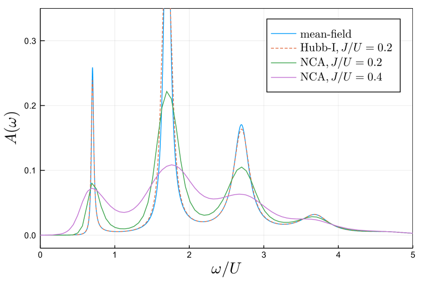
Figure 5: Local spectral function $A(\omega)$ for different values of $J/U$, as computed within Gutzwiller mean-field theory (blue line), DMFT with Hubbard-I impurity solver (dashed red line) and NCA impurity solver (green and violet full lines), for fixed $z=6$ and $r=0.6$. Gutzwiller results show a series of narrow peaks broadened by the local dissipation only. DMFT instead is able to capture additional broadening processes, already evident for $J/U=0.2$ within Hubbard-I, which however largely underestimates the effect of the non-Markovian bath as confirmed by the comparison with the more accurate NCA. Parameters: $dim_{H}=10$.

The Gutzwiller mean-field spectral function shows a series of narrow peaks, whose broadening is controlled only by the local dissipation. We remark that in this approach, corresponding to the infinite coordination number limit $z=\infty$, all properties of the normal phase are independent on the hopping and coincide with the single-site $J=0$ limit. Indeed as we have discussed in Sec. III.1, for $z=\infty$ the only feedback from neighboring sites comes through the order parameter $\mathbb{\Phi}$, which vanishes in this the normal phase.

DMFT instead is able to capture the effect of coherent hopping processes, resulting in a further broadening of the resonances. This finite hopping correction to the spectral function reflects the fact that the stationary density matrix in the normal phase is not a tensor product of single-site density matrices, as predicted by Gutzwiller, but rather includes correlations among neighboring sites encoded within DMFT in the non-Markovian bath.

A comparison between Hubbard-I and NCA, shows that the former largely underestimates the effect of the bath. Indeed within NCA the sharp peaks of the isolated single site problem are largely broadened already for a moderate value of the hopping rate $J/U=0.2$, a trend that further increases for larger values of $J/U$. At the same time the location of the poles is found to be weakly dependent on the hopping rate and, at least for $J/U=0.2$, essentially captured already by Hubbard-I and Gutzwiller mean-field. This difference can be understood by noticing that there are two main sources of resonance broadening within our DMFT approach, one coming from the bare non-Markovian bath $\Delta(\omega)$, the other coming from the Markovian interacting single-site problem, encoded in the self-energy $\Sigma(\omega)$ (see Sec. III.3). Within Hubbard-I the latter is independent of $J$, and only set by pump and losses. NCA on the other hand accounts for many body scattering channels mediated by the bath and results in an imaginary part of $\Sigma(\omega)$, also scaling with the hopping strength and responsible for the larger broadening. We emphasize that while the main effect of the DMFT bath in this regime is to broaden the resonances, this broadening is not uniform in frequency, i.e. it could not be reproduced by treating the DMFT bath with a Markov approximation. In fact, the self-consistent condition Eq. (16) implies that the spectrum of the DMFT bath is given by the local spectral function itself, namely it comes with a rich multi-peak structure in frequency which prevents the use of a simple Markovian approximation. Overall the spectral function in this low-drive, low-hopping normal region is very reminiscent of an equilibrium Bose Hubbard model in the Mott insulating phase Strand et al. (2015b), with Hubbard bands, describing doublon/holons and multiparticle excitations, which are partially filled by incoherent pump and dissipation. As we show in the next section, increasing the pump strength reveals a spectral feature which is instead unique to interacting driven-dissipative systems.

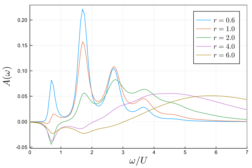
Figure 6: Local spectral function $A(\omega)$ obtained from DMFT/NCA for different values of the pump/loss ratio $r$ at fixed $J/U=0.2$ and $z=6$. Upon increasing $r$ the lowest Hubbard band flips sign and a region of Negative Density of States (NDoS) emerge at positive frequencies, up to $\omega=\Omega_{0}(r)$ where the spectral function vanishes, $A(\Omega_{0})=0$. The spectral range of NDoS increases with $r$. Parameters: $dim_{H}=14$.

V.1.1 Negative Density of States

We now discuss how the spectral features of the normal phase evolve upon increasing the strength of the drive/loss ratio $r$. While in the low pump regime all the peaks of the spectral function are positive, see Fig. 5, a novel effect appears at large drives. Above a threshold $r_{\rm ndos}$ the lowest Hubbard band flips sign and a region of Negative Density of States (NDoS) appears in a positive frequency range .

We show this in Fig. 6 where we plot the spectral function obtained within NCA/DMFT for different values of drive/loss ratio $r$, at fixed $J/U=0.2$. The region of NDoS extends up to $\omega=\Omega_{0}$, a frequency at which the imaginary part of the retarded Green’s function linearly vanishes, i.e. we have

$$A(\omega)=\gamma(\omega-\Omega_{0})\;\;\;\;\mbox{for}\;\omega\simeq\Omega_{0}$$ (40)

with $\gamma>0$, while for $\omega>\Omega_{0}$ the conventional positive sign is recovered. As we show in figure 6 the spectral range of NDoS increases with the drive $r$ and so does the frequency $\Omega_{0}(r)$. We stress that a negative spectral function at positive frequency is a genuine nonequilibrium phenomenon that cannot happen for closed systems in thermal equilibrium Scarlatella et al. (2018). It has a direct physical consequences on the response of the system to a weak local coherent drive oscillating at frequency $\omega$, $V(t)=\sum_{i}\left(v^{*}_{i}(t)b_{i}+\mbox{hc}\right)$ with $v_{i}^{*}(t)=v_{0}\delta_{i,0}\,e^{i\omega t}$. Indeed for an open system the power absorbed from the perturbation, defined as Alicki (1979); Feldmann and Kosloff (2003); Rivas (2020) $\dot{W}=\mbox{Tr}\rho(t)\dot{V}$ can be written within linear response theory as (see appendix D)

$$\dot{W}=v_{0}^{2}\omega A(\omega)$$ (41)

This expression highlights how the spectral function at frequency $\omega$ controls the power absorbed by the system under an external drive. A change in sign of this quantity, i.e. a negative absorbed power, signals the onset of energy emission and gain, a condition which is generally associated to optical amplification and lasing Scovil and Schulz-DuBois (1959); Boukobza and Tannor (2006, 2007); Liu et al. (2015). As we are going to discuss in Sec V.3 the NDoS effect and the frequency $\Omega_{0}$ will play a crucial role in the nonequilibrium phase transition from the normal to the superfluid phase.

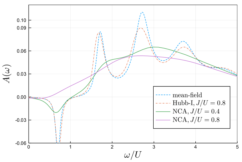
Figure 7: Local spectral function $A(\omega)$ for different values of $J/U$, as computed within Gutzwiller mean-field theory (dashed blue line), DMFT with Hubbard-I impurity solver (dashed red line) and NCA impurity solver (green and pink full lines), for fixed $z=6$ and $r=2$. Within NCA we see that increasing the hopping $J$ changes qualitatively the structure of the low frequency spectrum, washing out the NDoS and restoring a positive spectrum at $\omega>0$. This effect of the DMFT bath is completely missed by Gutzwiller mean-field as well as Hubbard-I approximations. Parameters: $dim_{H}=10$

We emphasize that the NDoS effect arises already in the single-site problem, i.e for $J=0$ in our model, above a threshold pump $r_{\rm ndos}$ which depends on the strength of Kerr nonlinearity, as discussed in Ref. Scarlatella et al. (2018). As a result, it naturally appears at large drive in the normal-phase spectral function of our lattice model calculated within Gutzwiller mean-field theory as well as DMFT/Hubbard-I, both built out of the exact solution of the single site problem.

We now discuss the dependence of the NDoS effect from the hopping $J$. Clearly such a question goes beyond Gutzwiller mean-field theory, which as we stressed cannot capture any effect due to coherent hopping within the normal phase. In figure 7 we plot the spectral function obtained with DMFT/Hubbard-I and NCA, for increasing values of $J/U$ and compare with the results obtained from Gutzwiller. We find that the NCA spectral function is strongly affected by the hopping, which broadens the sharp high-energy peaks and decreases the strength of the negative peak around $\Omega_{0}$, up to a value of $J/U\simeq 0.8$ at which this peak turns back to positive, washing away the NDoS effect. In other words NCA is able to capture a renormalization of the scale $\Omega_{0}$ from the hopping $J$. This is surprising at first since $J$ is a purely coherent energy scale while we have seen in Figure 6 that the strength of the peaks and the NDoS is controlled by the dissipative scales, i.e. the pump to loss ratio. We interpret this effect as a first example of hopping-induced losses, a mechanism that is unique to open quantum systems and that plays a key role in the physics of our model. Importantly, this effect is completely missed by the simple impurity solver Hubbard-I, whose spectral function, also shown in Figure 7, changes very little with respect to the Gutzwiller mean-field one  .

To summarize, we have seen that changing drive and hopping largely affects the spectral properties of the normal phase. In particular we have identified for positive frequencies $0<\omega<\Omega_{0}(r,J/U)$ a region of NDoS emerging above a threshold drive strength $r>r_{\rm ndos}(J/U)$. Both these quantities depend within DMFT/NCA from the hopping-to-interaction ratio $J/U$, an effect which is completely missed by Gutzwiller mean field as well as by Hubbard-I. As we are going to discuss in Sec. V.3, these dependencies of the critical frequency $\Omega_{0}$ and of the threshold drive $r_{\rm ndos}$ from the hopping strength $J$ will have direct consequences on the phase diagram of the model.

V.2 Steady State Local Density Matrix and Population Inversion

We now discuss the occupation properties of the stationary state distribution in the normal phase. For a lattice problem computing the full many-body density matrix can be done only for very small systems. Nevertheless, within our DMFT/NCA approach, describing the thermodynamic limit of infinitely-many sites, we can compute the reduced steady-state density matrix of a given site of the lattice, say site $i=0$, obtained by performing a partial trace on all other sites, namely $\rho_{s}=\text{tr}_{j\neq 0}\rho_{\rm latt,s}$. This corresponds to the steady-state density matrix of the DMFT self-consistent quantum impurity model (9) and thus of the non-Markovian map $\mathcal{\hat{V}}$ (28) and it obeys Eq. (37). This reduced on-site stationary density matrix allows to study the change of the local populations of bosons due to hopping processes, which is completely missed by Gutzwiller mean-field theory. Also, for open systems these hopping processes enable new, effective dissipative channels. For example a particle can be injected from the Markovian environment on one site, hop to another site and escape the system, rather than just being created and annihilated on the same site. Those processes are captured by our DMFT approach and mimicked by the non-Markovian environment $\Delta$ and unlock interesting new physics which we are going to discuss here.

V.2.1 Local Occupation vs J

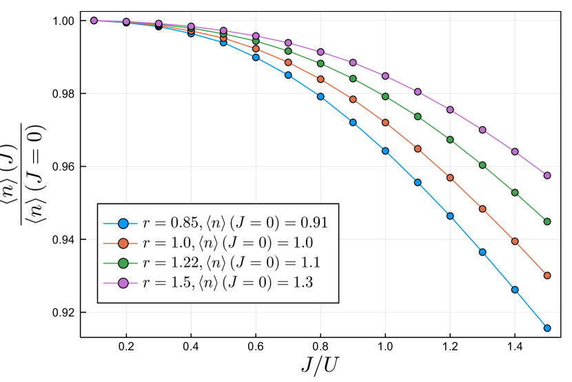
Figure 8: Local density of particles as a function of the hopping to interaction ratio $J/U$, within DMFT/NCA, for different values of the pump to loss ratio $r$, normalized to the values of the single site problem. We see that the density decreases with $J/U$, a specific feature of driven-dissipative lattices with two-body losses (see main text), which is captured by DMFT. Parameters: $z=50$, $dim_{H}=10$. The drive values used are marked on the y axis of Fig. 10.

From the knowledge of the on-site reduced stationary state density matrix $\rho_{s}$ we can obtain the average local density $\langle n\rangle=\text{tr}\left(b^{\dagger}b\rho_{s}\right)$. We notice that the local density can be also obtained from the Green’s functions, in particular from the Keldysh component at equal times

$$G^{K}(t,t)=-i\langle{\left\{b(t),b^{\dagger}(t)\right\}}\rangle=-i\left(2\langle{b^{\dagger}(t)b(t)}\rangle+1\right)$$ (42)

which gives consistently the same result in our NCA approach.

Within DMFT the local density acquires a dependence from the hopping $J$, which is obviously missing in Gutzwiller mean field. In Fig. 8 we plot the density as a function of $J/U$ at $z=6$ and for different values of the drive, normalised to the mean-field value ($z=\infty$). We see that quite generically the density decreases smoothly upon increasing the hopping within the normal phase, i.e. for $J<J_{c}$. This can be understood as an interplay of two particle losses and coherent hopping between neighboring sites, an effect that will be further explained by discussing the stationary-state populations in the next section. Interestingly the rate of decrease of the density with hopping changes quite strongly with the strength of the pump $r$ and in particular we notice in Figure 8 that a large drive seems to make the density more pinned to the single-site value.

The result in Fig. 8 turns out to be a specific feature of dissipative lattices with two-particle losses. In fact one can generically prove that for a driven-dissipative Bose-Hubbard model with only single particle losses and single particle drive the stationary state density matrix is independent of any Hamiltonian parameter Lebreuilly et al. (2016), leading to a density of particles independent of $J$ (although not necessarily integer, as it would be in the equilibrium Mott ground state of the Bose-Hubbard model ) and only set by drive/loss balance. In App. B we show that this effect is correctly captured by our DMFT/NCA approach, a highly non-trivial benchmark for its validity.

V.2.2 Steady-State Populations and Population Inversion

In this section we discuss the effect of coherent hopping processes on the steady state reduced density matrix, which as we show exhibits richer physics than the local occupancy. In the normal phase this quantity is diagonal in the basis of Fock states with $n$ bosons per site and the steady state populations $\rho_{n}$ are shown in Fig. 9 for different hopping values, $z=6$ and $r=3$.

First we observe that the single-site model, corresponding to $J=0$, shows a non-monotonic behavior of the populations as a function of the number of bosons per site, for drive/loss ratio $r>1$ and any value of the Kerr non-linearity $U$ (which in fact does not affect the stationary state as it is has been long known Dykman (1978)). This population inversion at $J=0$ appears clearly in Fig. 9, where the probability of finding $n$ bosons per site is maximum at $n=1$ despite the fact that a finite bosonic occupation costs energy $E_{n}=\omega_{0}n+Un^{2}/2\sim U$ and should be therefore thermodynamically suppressed.

Increasing the hopping changes the populations at low occupancy while leaving essentially unaffected the tail at large $n$. In particular, the coherent hopping from and into the neighboring sites increases the probability of having an empty site at expenses of finite occupation. This is a genuine feature of our dissipative many body lattice problem with local two body losses: starting from a state with average filling $n\sim 1$, hopping processes towards neighboring sites creates double occupations which escape at a rate $\eta$, reducing the total occupation. This trend goes on upon further increasing $J$, ultimately suppressing the population inversion above a threshold hopping. This mechanism also explains more in detail the observed overall decrease of average occupation with $J$, Fig. 8, which we already discussed in the previous section.

An interesting question concerns the relation between the NDoS effect discussed in Sec. V.1 and the population inversion in the reduced stationary density matrix. In closed quantum systems described by unitary evolution the two concepts are directly related, namely a NDoS could only emerge in presence of a inversion of populations where higher energy states are more occupied than lower energy ones. For open quantum systems the situation is more subtle and the two concepts are not in one-to-one correspondence Scarlatella et al. (2018).

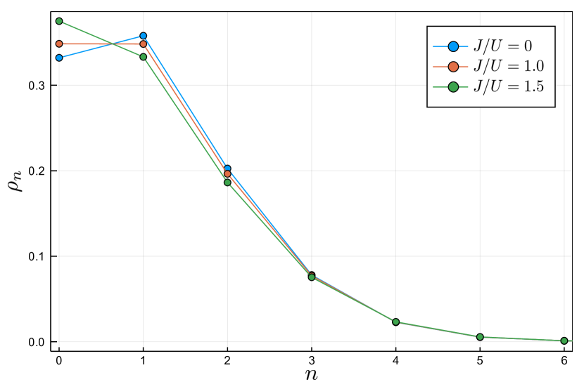
Figure 9: Steady state populations of the reduced density matrix $\rho_{n}=\langle n|\rho_{s}|n\rangle$, within DMFT/NCA, for different values of the hopping to interaction ratio $J/U$ and for $r=1.22$. We see that increasing $J/U$ changes the populations at low values of $n$ and ultimately washes away the population inversion found in the single site limit $J/U=0$. Parameters: $z=50$, $dim_{H}=10$. The drive value used is marked on the y axis of Fig. 10.

In Figure 10 we plot the behavior of the threshold for population inversion $r_{\rm inv}$ and for NDoS $r_{\rm ndos}$ as a function of $J/U$. We notice that those thresholds are independent from the hopping within Gutzwiller mean field (see dashed lines, which coincide with the $J=0$ values of DMFT) while they are substantially renormalized in DMFT. In particular the two scales $r_{\rm ndos}<r_{\rm inv}$ further deviates from each other as the hopping is increased. We note that $r_{\rm inv}$ increases monotonically with the hopping strength $J$ in DMFT. Based on closed systems arguments, this hopping-induced suppression of population inversion would suggest that the NDoS is also always suppressed by hopping, as for example Fig. 7 shows. Surprisingly, this is not always the case. Figure 10 shows that $r_{\rm ndos}$ has a non-monotonic behavior with the hopping rate $J$, namely its behavior changes from small and large hopping values. While for large values of $J$ the NDoS threshold $r_{\rm ndos}$ indeed increases following the behavior of the $r_{\rm inv}$ threshold, as expected from closed system arguments, for small values of $J$ it is actually reduced below the $J=0$ threshold, corresponding to the single site. Namely, for small values of $J$, the non-Markovian bath $\Delta$ actually generates a NDoS, even in a regime where the single site model would not present any signature of this effect. This is a unique feature of dissipative quantum systems, where an NDoS can be generated even in absence of population inversion. For Markovian systems it has been shown that this can be traced back to the structure of excitations on top of the stationary state, which come with characteristic complex weights, leading to anti-lorentzian lineshapes Scarlatella et al. (2018).

V.3 Finite Frequency Instability of the Normal Phase

In this section we discuss how the peculiar spectral and occupation properties of the normal phase contribute to an instability towards a spontaneous breaking of $U(1)$ symmetry. We show that the conventional static superfluid transition of the equilibrium Bose Hubbard model as a function of the hopping to interaction ratio $J/U$ is pushed to finite frequency as a result of drive and dissipation, leading to an order parameter oscillating in time. We emphasize the role of the NDoS for the onset of the phase transition and compare the DMFT/NCA and Gutzwiller phase boundaries. We argue that the effect of finite-connectivity fluctuations is not only quantitative, but rather underlines a qualitatively new physical mechanism for the onset of an ordered phase in open quantum lattices with two-body losses, which cannot be simply interpreted as the destruction of an ordered phase by thermal fluctuations in an effective equilibrium problem.

V.3.1 DMFT Phase Boundary

Within our DMFT approach, we can derive an equation for the phase boundary separating the normal and the broken symmetry phases. We assume to be in the early symmetry-broken phase, where the order parameter $\mathbb{\Phi}(t)=\langle{\mathbb{b}(t)}\rangle$ has just formed and it is small. This implies a small external field $\mathbb{\Phi}_{\text{eff}}(t)$ (14) in the DMFT effective action (9). We also assume to be in a stationary regime at long times, such that two point correlators depend only on time differences, and move to Fourier space. The average value of the bosonic field $\mathbb{\Phi}(\omega)\equiv\langle{\mathbb{b}(\omega)}\rangle$ is, to linear order in $\mathbb{\Phi}_{\text{eff}}$

$$\mathbb{\Phi}(\omega)=-\mathbb{G}^{R}(\omega)\mathbb{\Phi}_{\text{eff}}(\omega)$$ (43)

where we used the fact that $\langle{\mathbb{b}(\omega)}\rangle_{\mathbb{\Phi}_{\text{eff}}=0}=0$. A key point now is that at finite $z$ the effective field $\mathbb{\Phi}_{\text{eff}}(\omega)$ in DMFT has two contributions, one from the local order parameter itself and the other from neighboring sites encoded in the non-Markovian bath, see Eq. (14) which now reads (using $\mathbb{\Phi}_{+}=\mathbb{\Phi}_{-}$ as well as $\mathbb{\Phi}_{\text{eff}+}=\mathbb{\Phi}_{\text{eff}-}$ )

$$\mathbb{\Phi}_{\text{eff}}(\omega) =J\mathbb{\Phi}(\omega)+\mathbb{\Delta}^{R}(\omega)\mathbb{\Phi}(\omega)$$ (44)

Plugging (44) into (43) and using the DMFT self-consistency on the Bethe lattice (16) one finally gets

$$\mathbb{\Phi}(\omega)=\left(-J\mathbb{G}^{R}(\omega)-\frac{J^{2}}{z}\mathbb{G}^{R}(\omega)\mathbb{G}^{R}(\omega)\right)\mathbb{\Phi}(\omega)$$ (45)

The critical coupling $J_{c}$ and critical frequency $\Omega_{c}$ needed for a self-consistent broken-symmetry solution, $\mathbb{\Phi}(\Omega_{c})\neq 0$ corresponding to an order parameter whose phase oscillates in time $\langle b(t)\rangle\sim e^{-i\Omega_{c}t}$ for $J>J_{c}$, are given by

$$\frac{1}{J_{c}}+G^{R}(\Omega_{c},J_{c})+\frac{J_{c}}{z}\left[G^{R}(\Omega_{c},J_{c})\right]^{2}=0$$ (46)

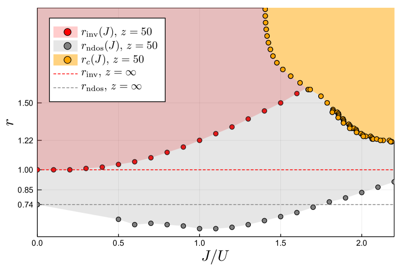
Figure 10: Threshold drives for NDoS $r_{\rm ndos}(J)$ and for population inversion in the density matrix $r_{\rm inv}(J)$, as a function of the hopping and compared with the critical drive $r_{\rm c}(J)$ (yellow points) for the finite-frequency superfluid transition. The ticks of the y axis correspond to the values of $r$ used for Figures 9 and 8. We see that for small value of $r$ the phase transition occurs even in absence of a population inversion, i.e. it is the NDoS the key effect leading to the instability of the normal phase. Parameters: $z=50$. Red curve: $t_{max}=10$, $dim_{H}=14$. Gray curve: $t_{max}=20$, $dim_{H}=10$.

Equation (46), which to the best of our knowledge is an original result of this paper, is generic for bosonic DMFT theories on the Bethe lattice and it holds also for equilibrium problems. Its solution, leading to the phase boundary in Figures 2 and 10, strongly depends on the driven-dissipative nature of the problem, as we are going to discuss now. First, Eq. (46) has real and imaginary parts, which both need to vanish simultaneously, resulting in the two conditions

$$\text{Im}G^{R}(\Omega_{c},J_{c}) =0$$ (47)

$$\frac{1}{J_{c}}+\text{Re}G^{R}(\Omega_{c},J_{c})+\frac{J_{c}}{z}\left[\text{Re}G^{R}(\Omega_{c},J_{c})\right]^{2} =0$$ (48)

We remark that there is another solution possible, where $\text{Im}G^{R}(\Omega_{c},J_{c})\neq 0$, but this is never realized in our simulations. In thermal equilibrium the first condition Eq. (47) can be only satisfied at zero frequency, where fluctuation-dissipation theorem constraints the imaginary part of a bosonic retarded Green’s function to vanish, thus allowing for static symmetry breaking patterns (as in equilibrium superfluids). Far from equilibrium this does not need to be the case Keeling et al. (2010); Scarlatella et al. (2019) and indeed we have seen that the normal phase shows, above a threshold drive $r_{\rm ndos}$, a spectral function vanishing at a positive frequency, corresponding to the formation of a NDoS and the onset of gain in the system. The critical frequency $\Omega_{c}$ solving Eq. (47) corresponds therefore to the frequency at which the local spectral function of the normal phase vanishes

$$\Omega_{c}=\Omega_{0}(r,J_{c}(r))$$ (49)

for a critical value of hopping $J_{c}$ determined by jointly solving Eq. (48). The energy scale $\Omega_{0}$ for the NDoS is therefore a precursor of the mode that will become unstable at the transition. We conclude that the NDoS effect discussed in previous section is a key, necessary condition for a phase transition into the nonequilibrium superfluid phase. This is clearly shown in Figure 10, where we plot the threshold pump $r_{\rm ndos}$ for NDoS and the critical drive $r_{c}$ obtained from solving Eq.  (46) with DMFT/NCA as a function of $J/U$. We see that generically $r_{\rm ndos}<r_{c}$, namely the system first develops gain and then becomes truly unstable towards $U(1)$ symmetry breaking. On the other hand, from Figure 10 we see that one can obtain an instability even in absence of population inversion.

V.3.2 Role of finite-connectivity fluctuations and comparison with Gutzwiller

We now go back to an important aspect mentioned at the beginning of our paper, namely the large renormalisation to the phase boundary obtained within DMFT/NCA upon decreasing the connectivity $z$. As we show in Figure 2 and Figure 11, fluctuations due to the finite-number of neighbors shift the phase boundary towards larger values of the hopping $J$ and pump/loss ratio $r$. We now provide a physical interpretation of this effect based on the properties of the normal phase discussed so far.

We start by considering the condition for the normal phase instability obtained within Gutzwiller mean-field theory, which corresponds to the $z\rightarrow\infty$ limit of the Eq. (46). In this limit the problem reduces to a quantum single site, while the feedback from neighboring sites is treated at a purely classical level (See Sec. III.1), in terms of a self-consistent coherent field which reads $\Phi_{\rm eff}=J_{c}\langle\mathbb{b}(t)\rangle\sim Je^{i\Omega_{c}t}$ near the instability. As such, if we repeat the argument of the previous section we can obtain a condition for the Gutzwiller phase boundary, which reads

$$\frac{1}{J_{c}(z=\infty)}+G_{0}^{R}(\Omega_{c}(z=\infty))=0$$ (50)

where the first term is the effective field contribution and $G_{0}^{R}(\omega)$ is the retarded Green’s function of the isolated single-site problem and is therefore independent from the hopping. Within Gutzwiller mean-field theory the hopping $J$ has only the role of triggering the symmetry breaking, through the self-consistent field $\Phi_{\rm eff}$, while the onset of gain is controlled by the pump to loss ratio $r$. Indeed we known that the single site spectral function develops a NDoS above a constant threshold pump $r_{\rm ndos}$ (see gray dashed line in Figure 11). The feedback from the neighboring sites acts as a seed for a single site which is on the verge of energy emission (negative absorbed power at $\Omega_{c}$, see Eq. (41)) and leads, above a threshold hopping $J_{c}$ shown in Figure 11, to amplification of the local coherent field at frequency $\Omega_{c}$ and a spontaneous breaking of $U(1)$ and time-translation symmetry. Interestingly, the Gutzwiller phase boundary is very close to the line $r_{\rm ndos}$ (see Figure 11) suggesting that at large hopping as soon as the system develops gain the symmetry breaking occurs.

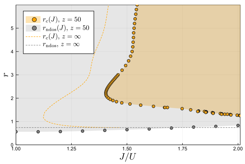
Figure 11: Phase diagram in the pump versus hopping plane obtained by DMFT/NCA for $z=50$ (yellow points) and Gutzwiller mean field theory ($z=\infty$, yellow dashed line). We further plots the thresholds for NDoS obtained within the two approaches. We see that fluctuations due to finite connectivity reduce the broken symmetry phase, pushing it towards higher values of hopping and drive. We interpret this effect as a signature of hopping-induced losses, which reduce the local gain and prevents the system to become unstable at finite frequency. Parameters :$dim_{H}=10$

DMFT/NCA on the other hand accounts for a more subtle effect of neighboring sites, which are encoded in the non-Markovian quantum bath, in addition to the classical coherent field. As we know this provides an increased effective dissipation, due to hopping processes from lossy neighboring sites, which is responsible for wiping out the NDoS region in the local spectral function, a necessary condition for the onset of the instability. This is clearly shown in Figure 10 where for large values of $J/U$ the threshold for NDoS eventually becomes larger than the Gutzwiller mean-field one (see gray dashed line in Figure 10), leaving a normal phase which would be superfluid at $z=\infty$. These hopping-induced losses provide therefore a clear physical mechanism behind the finite-connectivity renormalization of the phase boundary. The picture that emerges from DMFT is the one of a single site on the verge of energy emission, coupled to an oscillating seed field which would favor optical amplification and embedded in a non-Markovian bath which is instead able to absorb part of the emitted power from the system, thus reducing the effective gain and requiring a stronger value of pump to trigger the instability. This mechanism is presumably also effective at intermediate value of the hopping where, as we see in Figure 11, the DMFT/NCA threshold for NDoS remains well below the critical drive responsible for the true many-body instability at intermediate coupling, while approaching it at large hopping.

We conclude that this hopping-induced dissipation is a qualitatively new mechanism for the destruction of an ordered phase, which is unique to open systems settings and one of the hallmark of our DMFT/NCA approach. Quite interestingly this mechanism is not only completely missed by the Gutzwiller mean field approach, but also by a perturbative solver such as the Hubbard-I approximation. In fact we have discussed (see in figure 7) how the NDoS is changed very little within this scheme. In appendix E we also show that the Hubbard-I phase diagram, obtained using the DMFT equation for the critical point (46), still reduces to the Gutzwiller mean-field one. This further highlights the non-perturbative nature of the fluctuations responsible for the observed renormalization of the NDoS and the importance of using a self-consistent scheme such as our NCA approach.

V.3.3 Thermal vs. Non-Thermal Origin of Finite Connectivity Fluctuations

A different perspective on the role of finite-connectivity fluctuations on the phase boundary can be obtained by looking at the occupation of single particle modes at finite frequency, describing excitations on top of the stationary state and their effective thermal character. In fact, in an effective equilibrium picture, one could expect heating to provide an efficient mechanism for the reduction of a broken symmetry phase. To investigate this physics we look at the Keldysh Green’s function, defined in Eq (42), which heuristically describes the fluctuations of the observable ${b}$. If the system was in true thermal equilibrium, the quantum fluctuation-dissipation theorem (FDT) would constrain the Keldysh and the retarded components to obey the relation Kamenev (2011)

$$\frac{G^{K}(\omega)}{-2\pi iA(\omega)}\equiv F_{\rm eq}(\omega)=\coth\left(\frac{\omega}{2T}\right)$$ (51)

where $T$ is the system temperature. At low frequency or high temperatures, $\omega\ll T$, one has $F_{eq}(\omega)\sim T/\omega$. In a non-equilibrium system on the contrary there is no well-defined temperature and the FDT does not hold in general. Nonetheless, it is useful to use the left-hand side of the FDT relation in Eq. (51) to define an effective distribution function

$$F_{\rm neq}(\omega)=\frac{iG^{K}(\omega)}{2\pi A(\omega)}$$

and to study its frequency dependence.

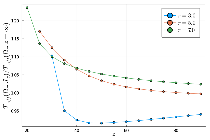
Figure 12: Change of the effective temperature $T_{\rm eff}$ at the critical point $(\Omega_{c},J_{c})$ as a function of lattice connectivity $z$, with respect to its mean-field value at $z=\infty$, for different values of the pump to loss ratio $r$. We see that the relative change in $T_{\rm eff}$ remains of the order of few percents up to connectivity $z=50$ and slightly increases up to $20\%$ for the lowest connectivity $z=20$. This should be compared to the DMFT renormalization of the critical hopping for similar values of drive and connectivity, which is instead much stronger as shown in Figure 2. In particular for $z=30$ and $r=3$ the critical hopping is pushed to infinity corresponding to a complete destruction of the normal phase. Parameters : $dim_{H}=14$.

Within the DMFT and Gutzwiller normal phases, for pump above the threshold for NDoS $r>r_{\rm ndos}$, the spectral function $A(\omega)$ vanishes at frequency $\Omega_{0}$, with linear corrections (see Eq. (40 ). On the other hand we find that the Keldysh component has a finite non-zero value at $\Omega_{0}$, which gives a distribution function of pseudo-equilibrium form at least for the modes around $\Omega_{0}$

$$F_{\rm neq}(\omega)\simeq\frac{T_{\rm eff}}{\omega-\Omega_{0}}$$ (52)

From this expression we can therefore identify an effective temperature $T_{\rm eff}$, which emerges quite ubiquitously in nonequilibrium quantum systems Mitra et al. (2006); Clerk et al. (2010); Foini et al. (2011); Dalla Torre et al. (2012); Schiró and Mitra (2014); Sieberer et al. (2016). At $z=\infty$, when the normal phase is described as a collection of independent sites, an effective temperature emerges due to the interplay of local drive and Kerr interaction Scarlatella et al. (2018). Within DMFT/NCA one could in principle expect important corrections due to the non-Markvovian bath, as we have seen for the NDoS. To assess this point we sit at the phase boundary, $J_{c}(r)$, choose the corresponding critical frequency $\Omega_{0}(J_{c},r)=\Omega_{c}$ and plot the behavior of $T_{\rm eff}$, scaled with respect to the $z=\infty$ value, as a function of the lattice connectivity $z$ and for different values of the pump-to-loss ratio $r$. We see that at large values of $r$ the effective temperature slightly increases upon decreasing $z$, while at smaller pumps, i.e. $r=3$, it shows a weak non-monotonic behavior with $z$. Overall, the relative variation of $T_{\rm eff}$ with respect to the Gutzwiller mean-field value remains rather moderate. On the other hand, in the same range of variation of $z$, the DMFT critical hopping shows instead strong renormalizations. This is particularly true for the small drive regime, where already for $r=3$ and $z=30$ the ordered phase is completely washed out. This observation suggests that effective thermal fluctuations and heating are not enough to explain the large renormalization of the phase diagram observed in DMFT, which is instead mainly driven by the reduction of local gain by virtual hopping processes, through the mechanism of hopping-induced losses.

V.4 Nonequilibrium Superfluidity, Lasing and Many Body Synchronization of Van der Pol Arrays

We now discuss how the nonequilibrium superfluid transition in our Bose-Hubbard model is connected to other dynamical phenomena associated with breaking of time-translation symmetry, such as nonequilibrium Bose-Einstein condensation, lasing and synchronization of Van der Pol oscillators. To appreciate this point it is useful to start from the semiclassical limit of our model (See Appendix C) where non-linear quantum fields contributions) are disregarded. The dynamics of the bosonic field at site $j$ takes the form of a Langevin equation

$$i\dot{b}_{j\rm cl}=\left(\tilde{\omega}_{0}(b_{j\rm cl})+i\gamma(b_{j\rm cl})\right)b_{j\rm cl}+\frac{J}{z}\sum_{\langle j^{\prime}\rangle}b_{j^{\prime}\rm cl}+\xi_{j}(t)=0$$ (53)

with an effective frequency and damping terms which depend non-linearly on the field itself, i.e. $\tilde{\omega}_{0}(b_{j\rm cl})=\omega_{0}+U|b_{j\rm cl}|^{2}/2$ and $\gamma(b_{j\rm cl})=f/2-\eta|b_{j\rm cl}|^{2}/2$, and where $\xi_{j}(t)$ is a zero average white noise $\langle\xi_{i}(t)\xi_{j}(t^{\prime})\rangle=f\delta(t-t^{\prime})\delta_{ij}$. In the continuum limit this reduces to a complex Gross-Pitaevski equation Pitaevskii and Stringari (2016); Aranson and Kramer (2002) with pump and non-linear losses which describes a variety of non-linear phenomena from exciton polariton condensates to multi-mode lasers Keeling and Kéna-Cohen (2020). In absence of any noise the spatially uniform stationary state admits a stable limit cycle, i.e. $\beta(t)=|\beta|e^{-i\omega_{\rm vdp}t}$ for $r>0$ and any $J$ with frequency $\omega_{\rm vdp}$

$$\omega_{\rm vdp}=\omega_{0}-J+U|\beta|^{2}/2$$ (54)

and amplitude set by the incoherent drive, $|\beta|=\sqrt{r}$.Equation (54) is therefore the semiclassical version of our condition for finite-frequency instability in the normal phase. A major difference exists between the lasing threshold and our case, namely that the threshold for the onset of gain and the one for development of full coherence is well separated, while it coincides in the usual lasing regime Keeling et al. (2010). This can be seen easily by looking at the Green’s function which develops a NDoS as soon as the system becomes unstable.

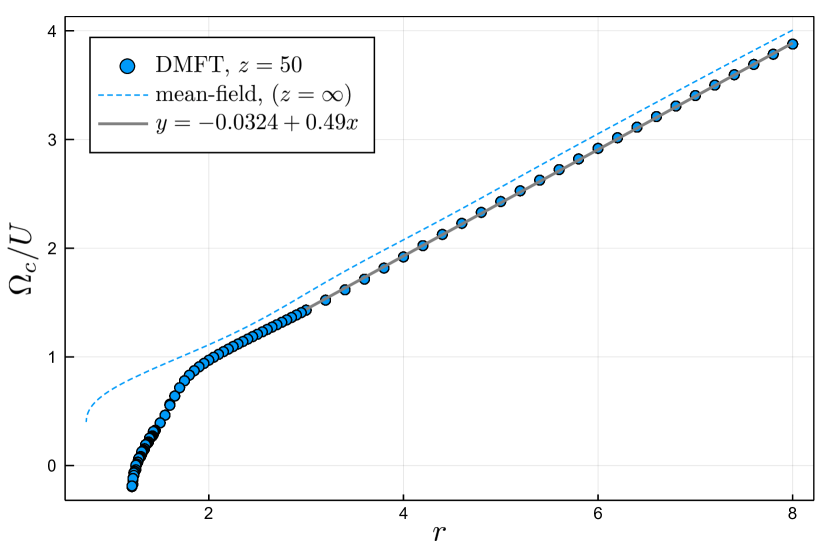
Figure 13: Critical frequency for quantum synchronization $\Omega_{c}$ as a function of the pump/loss ratio $r$, within DMFT/NCA for connectivity $z=50$ and Gutzwiller mean field theory ($z=\infty$). In the region of large drive the fit shows that $\Omega_{c}/U\sim r/2$, in agreement with the semiclassical result for the limit cycle in the VdP array. At lower drives, in the regimes of few bosons per sites, quantum fluctuations become relevant and the critical frequency is strongly renormalized. Parameters: $dim_{H}=14$.

The equation above describe also an array of coupled classical Van der Pol oscillators. Our driven-dissipative Bose-Hubbard model can be therefore also seen as a quantum many-body version of the VdP array. From this perspective, the onset of finite-frequency oscillations at $J_{c}(r)$ described in the last section can be seen as a signature of a quantum synchronization  Lee and Sadeghpour (2013); Lörch et al. (2016); Walter et al. (2014, 2015); Roulet and Bruder (2018a, b); Dutta and Cooper (2019); Giorgi et al. (2012); Manzano et al. (2013); Qiao et al. (2018); Sonar et al. (2018); Jaseem et al. (2020); Tindall et al. (2020), where above a certain coupling $J$ all quantum VdP oscillators enter into a collective limit-cycle phase. As we are going to discuss next, these oscillations share qualitative features with the semiclassical solution at least at large drive values, while deviate significantly for smaller drives where quantum fluctuations are important.

Despite the similarities the semiclassical limit described above is rather different from the large connectivity limit: in the former case one has a deterministic non-linear equation and desynchronization can only appear due to the noise. In the latter instead, corresponding to DMFT, one reduces to a quantum VdP oscillator coupled to a self-consistent field and a quantum bath. This is responsible for the large separation between the onset of gain and the true instability.

V.4.1 Critical Frequency versus Drive/Loss Ratio and Kerr Non-Linearity

In this section we discuss the behavior of the critical frequency $\Omega_{c}$, signaling the onset of a quantum synchronized phase, as a function of pump/loss ratio $r$ and Kerr non-linearity $U$. In Figure 13 we plot this frequency as a function of the incoherent drive amplitude $r$, both for DMFT (for $z=50$) and for Gutzwiller mean field theory ($z=\infty$). We see that $\Omega_{c}$ scales linearly with the drive at large values of $r$ (see fit in Fig. 13), a result which is in agreement with the semiclassical result obtained for the VdP array Eq. (54) where $\omega_{\rm vdp}/U\sim r/2$.

As the pump is reduced and the number of bosons per site decreases one expects quantum fluctuations to become more important. Indeed we see significant deviations from the semiclassical result at small $r$, already captured by Gutzwiller mean field but more pronounced for DMFT.

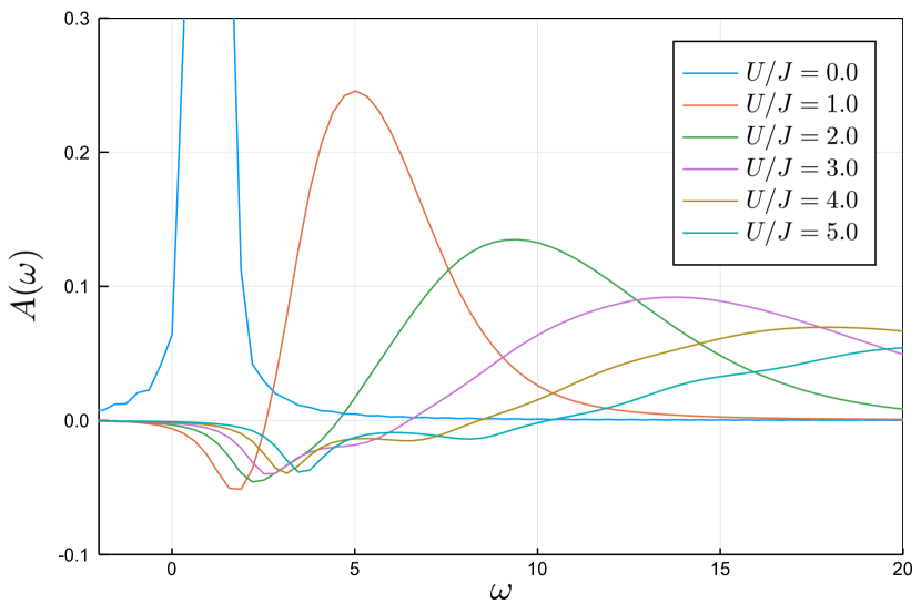
Figure 14: Local spectral function $A(\omega)$ for increasing values of the Kerr non-linearity $U$, at fixed value of hopping $J=\omega_{0}$ and drive-to-loss ratio $r=3$ within DMFT/NCA. We see that the frequency $\Omega_{0}$ at which the density of states vanishes, decreases with $U$ and eventually disappears for small enough values of $U$. Parameters: $z=6$, $dim_{H}=14$.

Another interesting aspect is the role played by the Kerr non-linearity. In Fig. 14 we plot the local density of states for fixed value of hopping and drive/loss ratio and for different values of the interaction $U$. A first interesting observation is that the frequency $\Omega_{0}$ at which NDoS emerges, related to the mode becoming critical at the synchronization transition (see Eq. (49), decreases upon reducing the Kerr non-linearity. A detailed analysis shows $\Omega_{c}\sim U$. We notice the analogy with the semiclassical result (54), nevertheless we stress that in this picture the critical frequency is proportional to the modulus square of the order parameter $|\langle b\rangle|^{2}\neq 0$, while within DMFT we find $\Omega_{c}\sim U$ at the critical point, where by definition $\langle b\rangle=0$ . This further highlights the quantum nature of the synchronization transition considered in this work. Indeed we have seen how $\Omega_{c}$ is smoothly connected to the frequency $\Omega_{0}$ where NDoS emerges, a scale that exists already well inside the normal incoherent phase and that is a genuine feature of the quantum impurity model. Furthermore this implies that the Kerr non linearity is crucial in order to push the transition at finite frequency, implying undamped oscillations of the order parameter. We indeed observe that for a related model of all-to-all coupled quantum VdP oscillators recent Gutzwiller mean-field analysis reported a static (first-order) transition in absence of any Kerr non-linearity Lee and Sadeghpour (2013); Davis-Tilley et al. (2018).

We conclude by noting that an oscillating phase in the order parameter could be in principle gauged away by going to an appropriate rotating frame. This however could not be done a priori, since as we have seen the critical frequency $\Omega_{c}$ itself depends from the many-body physics of the problem. We are considering here only the instability of the normal phase, rather than the dynamics in the full broken symmetry phase which could show a more complex dynamical behavior, whose description goes beyond the scope of the stationary-state oriented approach (see Sec. IV.2.1) used here.

V.4.2 Limit Cycles at Finite Connectivity

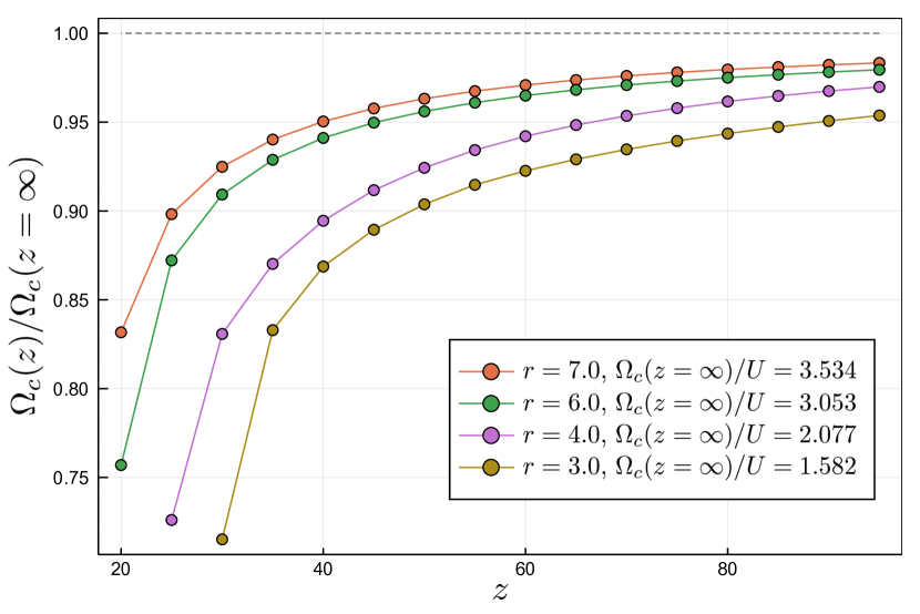
Figure 15: Critical Frequency for quantum synchronization, $\Omega_{c}$, within DMFT/NCA, as a function of the lattice connectivity $z$, for different values of the drive-to-loss ratio $r$ and hopping fixed on the phase boundary $J/U=(J/U)_{c}$. For clarity we normalize $\Omega_{c}$ to the mean field value obtained for $z=\infty$. We see that decreasing $z$ renormalizes down the frequency, but does not destroy the limit cycle. Parameters: $dim_{H}=14$.

Limit-cycles emerge ubiquitously within mean field approaches Lee et al. (2011); Chan et al. (2015); Wilson et al. (2016); Schiró et al. (2016), and indeed even in the present problem the Gutzwiller solution at $z=\infty$ predicts one. The role of fluctuations on their stability has been discussed before, in particular in the context of a coherently driven anisotropic Heisenberg model with spontaneous decay  Owen et al. (2018). There an approach based on self-consistent Mori projection Degenfeld-Schonburg and Hartmann (2014) and cluster mean field Jin et al. (2016) predicts that limit cycles disappear as the coordination number $z$ is decreased below a threshold value $z^{*}$ which depends on the system parameters.

On the basis of these results, it is particularly interesting to study the fate of our synchronization transition beyond Gutzwiller mean-field theory. In Fig. 15 we plot the behavior of the critical frequency $\Omega_{c}$ obtained from DMFT/NCA, as a function of $z$ for different value of $r$. We observe that finite $z$ corrections tend to reduce the value of $\Omega_{c}$ with respect to the mean field value, which nevertheless remains finite down to the lowest value of connectivity at which, for a given value of drive, a synchronization transition exists, consistently with the phase boundary moving to higher values of $r$ for decreasing $z$ (see Fig. 2). In other words we find that, within our treatment, finite connectivity does not destroy the limit cycle phase which is only pushed at higher values of the incoherent drive. Indeed in Fig. 15 we show that for drive $r=7$, the highest value that we can numerically access given the constraints on the local Hilbert space truncation, a limit cycle would exists down to $z=20$. We therefore expect that at higher drives the synchronized phase would survive down to low connectivity values. The regime of strong drive is however difficult to access within NCA and we leave this question open for future works. We remark nevertheless that our model is different from the one of Ref. Owen et al. (2018). In the present case the existence of a limit cycle phase is tightly related to a $U(1)$ symmetry present in the original Lindblad problem and spontaneously broken at the transition Scarlatella et al. (2019).

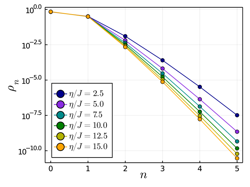
Figure 16: Quantum Zeno regime. Occupation probabilities of theDMFT/NCA on-site reduced density matrix $\rho_{n}=\langle n|\rho_{s}|n\rangle$, as a function of the number of number of particles per site and for different values of two-particle-loss rates $\eta/J$. For large $\eta/J$ we see that probabilities $\rho_{n\geq 2}$ are suppressed exponentially (note the log scale), with a rate that increases with $\eta/J$, while the states with $n=0,1$ bosons, not affected by the losses, retain a population of order one.

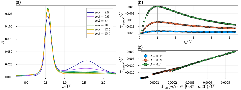
Figure 17: Quantum Zeno regime in the spectral function, increasing two-particle loss rate $\eta$ at fixed drive rate $f/U=r\eta/U=0.013$. Parameters: $t_{\rm max}=20$, $dt=0.002$, ${\rm dimH}=6$. (a) Spectral function at increasing $\eta/J$. The first peak corresponds to transitions between states with on-site occupation $n=0$ and $n=1$, while higher energy peaks are suppressed at large $\eta/J$. We fit the first peak as described in the main text in order to extract a measure of its lifetime $\gamma$. (b) Partial lifetime $\gamma_{\rm zeno}/U$ of the first peak of the spectral function obtained by removing the zero hopping and zero drive/dissipation contributions. We show that this quantity has a non-monotonic behaviour, analogous to the populations in Fig. (3), manifesting a quantum Zeno behaviour in the lifetime of excitations of the steady-state. (c) $\gamma_{\rm zeno}/U$ depends only on the dissipative scale $\Gamma_{\rm eff}/U$, analogously to the occupation probability $\rho_{1}$ as shown in the inset of Fig. (3).

V.5 Quantum-Zeno Regime

In the previous sections we have seen that the key feature of DMFT is the ability to capture hopping-induced dissipative processes in the normal phase, which are missed by Gutzwiller mean-field theory and ultimately responsible for the large corrections to the phase boundary due to finite connectivity. In this section we discuss a different parameter regime of our model, corresponding to large two-particle losses $\eta\gg J$, which alllows us to highlight even more the qualitative difference between DMFT and Gutzwiller predictions. In the large two-particle losses limit, and in absence of any external drive, a perturbative analysis has shown that the dissipative dynamics of the Bose-Hubbard model effectively takes place in the subspace with zero and one boson per site, which are dark states of the local dissipator García-Ripoll et al. (2009). These emergent hard-core bosons are subject to next-neighbor losses controlled by the scale

$$\Gamma_{\rm eff}=\frac{2(J/z)^{2}}{U^{2}+\eta^{2}}\eta$$ (55)

This effective dissipation is hopping-mediated – namely it is non-zero only at finite hopping $J$ – and remarkably it shows a non-monotonic behaviour as a function of the physical dissipation $\eta$: for $\eta\ll U$, it increases linearly with $\eta$. Instead, when $\eta\gg U$, the effective dissipation $\Gamma_{\rm eff}$ is suppressed by increasing the physical dissipation $\eta$. The latter is a quantum-Zeno regime Misra and Sudarshan (1977); Beige et al. (2000), in which the coherent hopping dynamics bringing the system outside of the hard-core bosons subspace is suppressed due to the large coupling to the environment García-Ripoll et al. (2009). In absence of an external pump the effective loss rate (55) ultimately leads the system to a zero density state and the Zeno scale 55 manifests itself in the transient dynamics García-Ripoll et al. (2009); Rossini et al. (2020). Here instead we demonstrate how, in presence of a small pump, the Quantum Zeno regime emerges in the stationary state properties of the system and how this effect is completely missed by Gutzwiller, even at a qualitative level, while captured by our DMFT/NCA approach.

We consider the regime of $\eta\gg J$ and a parametrically small pump rate $f\ll\eta$. In this case we expect the local occupation of all the states with more than one boson per site to be largely suppressed upon increasing the two-particle losses, since the small residual pump is not sufficient to counterbalance the losses. This is indeed shown in Fig. 16 where we plot the occupation probabilities of the on-site reduced density matrix obtained from DMFT/NCA and see that only the occupation of the states $n=0,1$ remain of order one, while $\rho_{n\geq 1}$ is exponentially suppressed. We emphasize that in this case the long-time limit of the problem remains non-trivial within this subspace, due to the interplay between the small residual pump and the coherent dynamics generated by the Hamiltonian. In Figure 3 we have shown that our DMFT/NCA approach is able to capture the emergence of a stationary Zeno regime, through a non-monotonic behavior of the steady-state probability of having exactly one bosons per site, namely $\rho_{1}$, versus $\eta/U$, showing a universal collapse when plotted against $\Gamma_{\rm eff}$. This is remarkable, since the dissipative scale in Eq. (55) describes particle losses which are non-local in space García-Ripoll et al. (2009) which a priori could have been expected to be beyond reach for a local approach such as DMFT. Instead, the non-Markovian bath is able to capture this hopping-induced dissipative processes. We emphasize that DMFT goes beyond the effective hard-core model of Ref. García-Ripoll et al., 2009 in that the full crossover from normal to Zeno phase is captured as $\eta/J$ is increased. In this sense we can see DMFT as providing a non-perturbative solution of the effective hard-core model in the limit of large lattice connectivity.

The presence of Zeno scale $\Gamma_{\rm eff}$ in the system not only affects the steady state populations, but is also expected to influence the lifetime of excitations of the steady-state, which can be extracted from the Green functions computed in DMFT. In Fig. 17 (a) we show the behaviour of the spectral function, defined in Eq. (39), for increasing $\eta/J$. We work in a regime in which $U$ is large so that different resonances in the spectrum, corresponding to single-particle transitions between states with occupation $n$ and $n+1$, are well separated Scarlatella et al. (2018). By increasing $\eta/J$ all the peaks but the first one decrease in amplitude, as the former are proportional to the occupation of states with $n\geq 2$, which decreases with $\eta$ (see Fig. 16). The amplitude of the lowest frequency peak, instead, increases with $\eta$ due to the increased probability of being in the subspace with occupation $n=0,1$. We concentrate on this peak in order to extract its width. In order to do so, we fit the peak with a generalized Lorentzian $A(\omega)=a\frac{(\omega-\omega_{0})b+1}{(\omega-\omega_{0})^{2}+\gamma^{2}}$, with fitting parameters $a,b,\gamma$, which exactly describes the shape of the peak at zero hopping and which approximates it at small hopping, whose lifetime is given by the fitting parameter $\gamma$.

We remark that the width $\gamma$ of the first peak has three contributions, $\gamma=\gamma_{\rm{diss}}+\gamma_{\rm{coh}}+\gamma_{\rm{zeno}}$. The first term comes from dissipation and pump at zero hopping $\gamma_{\rm{diss}}=\gamma(J=0,\eta,f,U)$ and it can be well estimated with perturbation theory Scarlatella et al. (2018), which shows it does not depend on $\eta$, as the transition $n=0\rightarrow n=1$ is unaffected by the two-particle losses at $J=0$. The second contribution to the lifetime is given by the hybridization of the energy levels of different sites at finite hopping, which is a purely coherent effect, independent of drive and dissipation. For example, this effect is responsible for the formation of the holon and doublon bands in the local spectral functions of the isolated Bose-Hubbard model, see e.g. Strand et al. (2015b). We call this term $\gamma_{\rm{coh}}=\gamma(J,\eta=0,f=0,U)$.

Finally, we expect a contribution coming from the hopping-induced decay, which we call $\gamma_{{\rm zeno}}$, which is present only for finite hopping and dissipation/drive. In Figure Fig. 17 (b), we show that the latter contribution follows a similar non-monotonic behaviour as $\Gamma_{\rm eff}$ as a function of $\eta/U$, witnessing the presence of quantum-Zeno behaviour in steady-state excitations. Analogously to populations, in Fig. 17 (c) we show that plotting $\gamma_{{\rm zeno}}/U$ as a function of $\Gamma_{\rm eff}/U$, the data points at different values of $J/U$ all collapse on the same curve, demonstrating that $\gamma_{{\rm zeno}}$ only depends on $J$ and $\eta$ through $\Gamma_{\rm eff}$.

VI Conclusions

In this paper we formulated the Dynamical Mean Field Theory for bosonic open quantum many-body systems described by a Lindblad master equation on the lattice. This method is based on a systematic expansion in the limit of large lattice connectivity $z$. Within DMFT, fluctuations due to finite lattice connectivity are treated non-perturbatively through the solution of a self-consistent quantum impurity model, which in our case amounts to a Markovian single-site problem coupled to a coherent field and to a non-Markovian quantum bath mimicking the rest of the lattice. The non-Markovian bath contains the key new ingredient of DMFT, which makes it different from the Gutzwiller mean-field theory, to which it reduces in the $z=\infty$ limit. In particular, with respect to the former, DMFT is able to capture both coherent and dissipative processes arising from the neighboring sites, the former playing a particularly crucial role in open quantum systems with correlated jump operators.

Using DMFT, together with a non-perturbative bosonic impurity solver based on a super-operator hybridization expansion truncated at the NCA level, we solved a Bose-Hubbard model in presence of two-particle losses and single particle pump, relevant for dissipative ultracold atoms as well as for arrays of superconducting circuits. We have shown that this model features a dissipative phase transition from an incoherent normal phase to a nonequilibrium superfluid, which occurs above a critical hopping or pump strength.

Within DMFT/NCA the phase boundary is strongly renormalized with respect to the Gutzwiller one, and pushed towards higher values of the couplings, leading to an increase of the normal phase. We have identified a new mechanism for this reduction of the broken symmetry phase which is unique to open quantum systems and arises from the suppression of local gain due to hopping-induced losses. This is a key feature brought forth by NCA, which treats the non-Markovian DMFT bath non-perturbatively, and it is instead missed by a simpler perturbative DMFT solver based on the Hubbard-I approximation. We have further discussed how the increased effective dissipation due to the finite number of lossy neighbors affects all the unusual properties of the DMFT/NCA normal phase, from the renormalization of the gain (NDOS) threshold and steady-state populations due to hopping, to the emergence of a stationary-state quantum Zeno regime for large two-body losses. These effects are all qualitatively missed by Gutzwiller mean-field theory.

Finally, we have shown that the transition into the nonequilibrium superfluid phase occurs at finite-frequency, corresponding to a local order parameter that oscillates in time at a frequency $\Omega_{*}$. Within DMFT/NCA this scale depends on both coherent and dissipative couplings, another important aspect which is missed by Gutzwiller mean-field theory. Drawing from the physics of quantum VdP oscillators we interpreted this phenomenon as the onset of quantum many body synchronization and limit cycles at finite lattice connectivity.

Our DMFT holds the promise to be applied to a variety of driven-dissipative quantum many body problems. Different bosonic models or driving schemes can be considered and readily studied with the NCA approach developed here, such as the recently introduced quadratically driven Kerr resonator Rota et al. (2019a), the coherently driven case explored in the context of quantum bistability Le Boité et al. (2013); Biondi et al. (2017b); Foss-Feig et al. (2017); Vicentini et al. (2018); Landa et al. (2020) or models relevant for the dissipatively stabilised Mott insulators of photons Ma et al. (2019). Interesting directions for the future involve the development of other quantum impurity solvers, made possible by the Markovian structure of the quantum impurity problem. In particular, one could go beyond the Non-Crossing Approximation by including higher-order diagrams or resumming the full hybridization expansion Schiro and Scarlatella (2019) with real-time diagrammatic Monte Carlo methods Schiró and Fabrizio (2009); Werner et al. (2009). Alternatively, one could map back the non-Markovian Keldysh action into a Lindbladian problem with a finite number of bath levels Arrigoni et al. (2013a) which could then be solved by exact diagonalisation Seclì et al. (2021), quantum trajectories, through a matrix product operator representations of the density matrix Strathearn et al. (2018); Kilda and Keeling (2019b) or using an extension of the numerical renormalization group Lotem et al. (2020). Further extensions of this approach could include the development of a cluster version of DMFT building upon recent developments for Markovian problems Jin et al. (2016).

Finally, we notice that a similar DMFT/NCA impurity solver, could be developed for driven-dissipative fermionic problems Arrigoni et al. (2013b); Panas et al. (2019) or quantum spins Otsuki and Kuramoto (2013), which are also being actively investigated and relevant for different experimental platforms Barreiro et al. (2011); Lee et al. (2013); Haller et al. (2015); Yamamoto et al. (2019); Nakagawa et al. (2020).

Appendix A Deriving DMFT for Open Markovian Quantum Systems

We present here a sketch of the derivation of the DMFT action and self-consistency conditions, using the quantum cavity method and following and extending Ref Strand et al. (2015a) to the open case. The main idea is to single out a given site of the lattice, $i=0$ in the following, and to write down its effective Keldysh action obtained after integrating out all the other sites.

$$i\mathcal{S}_{\text{eff}}[\bar{b}_{0},b_{0}]=\mbox{log}\int\prod_{i\neq 0}D\left[\bar{b}_{i},b_{i}\right]\,e^{i\mathcal{S}}$$ (56)

This effective single-site action describes, in principle, all the effects on site $i=0$ due to the coupling to the other sites by the hopping $J$, which, for our assumption of local jump operators and interactions (Sec. II), is the only term responsible for the coupling between different sites. To proceed, we notice that the full action Eq. (7) can be divided in three therms,

$$\mathcal{S}=\mathcal{S}_{0}+\delta\mathcal{S}+\mathcal{S}^{(0)}_{cav}\,$$

respectively $\mathcal{S}_{0}=\mathcal{S}[\bar{b}_{0},b_{0}]$ containing only the terms in Eqns. (7-8) involving fields at site $i=0$, a term $\delta\mathcal{S}$ containing the hopping terms to the $2z$ fields ($\bar{b}_{j},b_{j}$) at the neighboring sites

$$\delta\mathcal{S}=\frac{J}{z}\int dt\sum_{\alpha}\alpha\,\sum_{\langle 0j\rangle}\left(\bar{b}_{0\alpha}b_{j\alpha}+hc\right)$$ (57)

and a term $\mathcal{S}^{(0)}_{cav}$ describing a lattice with a cavity, namely including all the degrees of freedom except those at site $i=0$, see Figure 18. For an interacting many-body problem on a finite dimensional lattice integrating over the neighboring sites can only be done formally, as a cumulant expansion in $\delta S$, and leads to an effective action containing arbitrary powers of the local fields $\bar{b}_{0},b_{0}$, with coefficients given by the multipoints correlation functions of the cavity problem Georges et al. (1996). In the large connectivity limit, $z\gg 1$, one can formally organize this expansion in power of $1/z$ and obtain

$$\begin{split}\mathcal{S}_{\text{eff}}&[\mathbb{b}^{\dagger}_{0\alpha},\mathbb{b}_{0\alpha}]=S_{0}+\int dt\sum_{\alpha=\pm}\alpha\mathbb{\Phi}_{\text{eff}\alpha}^{\dagger}(t)\mathbb{b}_{0\alpha}(t)+\\ &+\frac{i^{2}}{2}\int dtdt\sum_{\alpha,\beta=\pm}\alpha\beta\,\mathbb{b}^{\dagger}_{0\alpha}(t)\mathbb{\Delta}^{\alpha\beta}(t,t^{\prime})\mathbb{b}_{0\beta}(t^{\prime})\end{split}$$ (58)

where, in order to allow for condensed phases, we have introduced the Nambu-spinor notation

$$\mathbb{b}^{\dagger}_{0}=\left(\begin{array}[]{l}b_{0}\;\bar{b}_{0}\end{array}\right)\,\;\;\mathbb{b}_{0}=\left(\begin{array}[]{l}b_{0}\\ \bar{b}_{0}\end{array}\right)$$

The coefficients entering the effective action (58) are related to quantum averages over the cavity action $\mathcal{S}^{(0)}_{cav}$

$$\mathbb{\Phi}_{\text{eff}\,\alpha}^{\dagger}(t)=J/z\sum_{\langle j0\rangle}\langle\mathbb{b}^{\dagger}_{j\alpha}(t)\rangle_{cav}^{(0)}$$ (59)

$$\mathbb{\Delta}^{\alpha\beta}(t,t^{\prime})=J^{2}/z^{2}\sum_{\langle j0\rangle\langle k0\rangle}\langle\mathbb{b}_{k\alpha}(t)\mathbb{b}^{\dagger}_{j\beta}(t^{\prime})\rangle^{(0)}_{cav}$$ (60)

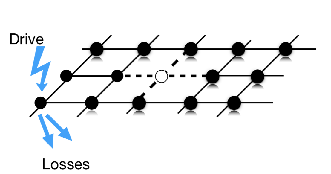
Figure 18: Sketch of the quantum cavity method to derive the effective action of DMFT for Markovian lattice problems (see text). A given lattice site is singled out (white dot in the figure) and all the remaining degrees of freedom are integrated out. Due to the coupling between the site and its $2z$ neighbors (dashed lines) this integration of degrees of freedom reduces to evaluate correlations function of a lattice with a cavity, containing all the remaining sites.

The final step, in order to obtain the self-consistent conditions, is to relate the average of bosonic fields on the cavity action to those evaluated to the effective action (58). For what concerns the non-Markovian bath in Eq. (60) this depends on the lattice geometry: it becomes particularly transparent for a Bethe lattice, a lattice with no loops such that once a cavity is created two neighbors $j,k$ are completely disconnected, where one gets

$$\langle\mathbb{b}_{k\alpha}(t)\mathbb{b}^{\dagger}_{j\beta}(t^{\prime})\rangle^{(0)}_{cav}=\delta_{kj}\langle\mathbb{b}_{j\alpha}(t)\mathbb{b}^{\dagger}_{k\beta}(t^{\prime})\rangle^{(0)}_{cav}=$$

$$=\delta_{kj}\langle\mathbb{b}_{j\alpha}(t)\mathbb{b}^{\dagger}_{j\beta}(t^{\prime})\rangle_{S}=\delta_{kj}\langle\mathbb{b}_{0\alpha}(t)\mathbb{b}^{\dagger}_{0\beta}(t^{\prime})\rangle_{S_{\rm eff}}$$ (61)

where we have used the property of the Bethe lattice in the first equality, the fact that in thermodynamic limit the local property of the cavity action and the original action must be the same in the second equality and translational invariance in the last step. Plugging this into Eq. (60) gives the self-consistency condition (16). We notice that simular arguments can be used for a different lattice, to relate averages over cavity and effective action, the only difference would be a more complicated self-consistency relation between bath and local Green’s function Georges et al. (1996). Finally, the average of the bosonic field taken on the cavity action can be related to the one on the effective action (58) as Strand et al. (2015a)

$$\langle\mathbb{b}^{\dagger}_{j\alpha}\rangle_{cav}^{(0)}=\langle\mathbb{b}^{\dagger}_{0\alpha}\rangle_{S_{\rm eff}}+$$ (62)

$$\int dt\,^{\prime}\sum_{\beta=\pm}\beta\langle\mathbb{b}^{\dagger}_{0\beta}(t^{\prime})\rangle_{S_{\rm eff}}\langle\mathbb{b}_{k\beta}(t^{\prime})\mathbb{b}^{\dagger}_{j\alpha}(t)\rangle^{(0)}_{cav}$$ (63)

which can be plugged in Eq. (59) to give the second self-consistent condition (14).

Appendix B NCA Benchmark: Local Occupation with Single-Particle Losses

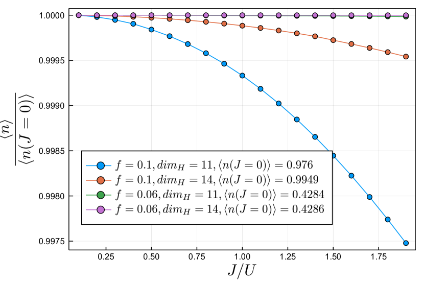
Figure 19: Local density of particles for the BH model with single-particle losses, as a function of the hopping to interaction ratio $J/U$, for different values of the drive amplitude $f$, normalized to the values of the single site problem. Parameters: $z=30$, $\kappa=0.2$, $dt=0.005$.

In this appendix we report a benchmark our DMFT/NCA approach for driven-dissipative many-body master equations defined by Eqs. (2) and (3). We consider a different model from the main text, namely the driven-dissipative Bose-Hubbard model with single-particle losses and single-particle drive. This is specified by the same Bose-Hubbard Hamiltonian Eqs. (3) and (4) as in the main text, but with the jump operators

$$\hat{L}_{i,l}=\sqrt{\kappa}\,\hat{b}_{i}$$ (64)

$$\hat{L}_{i,p}=\sqrt{f}\hat{b}_{i}^{\dagger}$$ (65)

where there is single-particle losses instead of the two-particle losses of the main text.

One can prove Lebreuilly et al. (2016) that the stationary state density matrix of this model is independent from any Hamiltonian parameter, thus, for example, the on-site occupation is constant with the hopping rate $J$. Obtaining this constant occupation with $J$ is a highly non-trivial benchmark for our DMFT/NCA approach. Figure 19 shows that this behavior is correctly reproduced by our approach. Small deviations from constant occupation show that this property is not exactly enforced by our numerical scheme and thus is a good test to validate our approach. Deviations from constant occupation are mostly a result of local Hilbert space truncation, which become more severe increasing the drive, but they are reduced by increasing the cutoff $\dim_{H}$.

Appendix C Keldysh Field Theory and Semiclassical Limit

In this section we write down the Keldysh field-theory associated to the Lindblad master equation for our driven-dissipative Bose-Hubbard model in Eq. (3-5). This is done by writing a coherent path-integral representation of the trace over the density matrix Kamenev (2011); Sieberer et al. (2016)

$$Z=\mbox{Tr}\rho(t)=\int\prod_{i}D\bar{b}_{i\rm cl}Db_{i\rm cl}D\bar{b}_{i\rm q}Db_{i\rm q}\,\exp\left(i\mathcal{S}\right)$$

in terms of bosonic fields in the classical-quantum basis $b_{j\rm cl/q}=\left(b_{j+}\pm b_{j-}\right)/\sqrt{2}$, where the Keldysh action reads

$$S=\int dt\sum_{j}\left[\bar{b}_{j\rm q}\left(i\partial_{t}-\omega_{0}-i\chi_{-}\right)b_{j\rm cl}+\mbox{hc}\right]-\frac{1}{2}\int dt\sum_{j}\left[\left(U+i\eta\right)\left(\bar{b}_{j\rm cl}^{2}b_{j\rm cl}b_{j\rm q}+\bar{b}_{j\rm q}^{2}b_{j\rm cl}b_{j\rm q}\right)+hc\right]+$$ (66)

$$+\int dt\sum_{j}\left(2i\chi_{+}-i\eta|b_{j\rm cl}|^{2}\right)\bar{b}_{j\rm q}b_{j\rm q}-\frac{J}{z}\int dt\sum_{\langle jj^{\prime}\rangle}\left([\bar{b}_{j\rm q}b_{j^{\prime}\rm cl}+hc\right)$$ (67)

where the first line describes the local non-interacting contribution, including the dissipative couplings $\chi_{\pm}=\left(\gamma_{p}\pm\gamma_{l}\right)/2$ which in the case considered in the main text, where $\gamma_{l}=0$ and $\gamma_{p}=f=r\eta$, reduce to $\chi_{\pm}=f/2$. The second line includes non-linearities due to interaction and two-body losses while the last term account for the hopping between neighboring sites. The semiclassical limit is obtained by disregarding terms with more than two quantum fields, which leaves the action at most quadratic in the quantum fields $b_{j\rm q}$ Sieberer et al. (2016). Those quadratic terms can be decoupled using a classical stochastic field Kamenev (2011) which allow to write the action as

$$S =\int dt\sum_{j}\left[\bar{b}_{j\rm q}\left(i\partial_{t}-\omega_{0}-i\chi_{-}+\xi_{j}(t)\right)b_{j\rm cl}+\mbox{hc}\right]+$$

$$+\left(U-i\eta\right)\int dt\sum_{j}\bar{b}_{j\rm q}|b_{j\rm cl}|^{2}b_{j\rm cl}+\mbox{hc}$$

$$-\frac{J}{z}\int dt\sum_{\langle jj^{\prime}\rangle}\left([\bar{b}_{j\rm q}b_{j^{\prime}\rm cl}+\mbox{hc}\right)$$ (68)

We can now take the saddle point conditions

$$\frac{\delta S}{\delta\bar{b}_{j\rm q}}=0=\frac{\delta S}{\delta\bar{b}_{j\rm cl}}$$

and obtain the Langevin equation given in Eq. (53) of the main text. We note that the non-interacting retarded Green’s function of the problem reads

$$G^{R}_{0}(\omega)=\frac{1}{\omega-\omega_{0}-i\chi_{-}}$$

which has NDoS as soon as $\chi_{-}\geq 0$, i.e. $r>0$ which is in the condition for the instability towards an oscillating solution.

Appendix D NDoS and Response to a Weak Coherent Drive

In this appendix we show that a direct consequence of the NDoS effect is that the average power absorbed from a weak coherent drive becomes negative, indicating the onset of gain and energy emission. We consider our lattice model in presence of a time dependent perturbation of the Hamiltonian describing a weak coherent drive with frequency $\omega$

$$H(t)=H+V(t)\equiv H+\sum_{i}\left(v_{i}^{*}e^{i\omega t}b_{i}+v_{i}e^{-i\omega t}b^{\dagger}_{i}\right)$$ (69)

where $H$ is the Bose Hubbard Hamiltonian defined in Eq.(3-4). The evolution of the density matrix of the system is described by the Lindblad master equation in presence of $H(t)$

$$\partial_{t}\hat{\rho}=-i[H(t),\hat{\rho}]+\sum_{i\mu}\left(\hat{L}_{i\mu}\hat{\rho}\hat{L}_{i\mu}^{\dagger}-\frac{1}{2}\left\{\hat{L}^{\dagger}_{i\mu}\hat{L}_{i\mu},\hat{\rho}\right\}\right)$$ (70)

We notice that the time derivative of the internal energy $E(t)=\langle H(t)\rangle$ in an open quantum system has two contributions, respectively coming from the derivative of the system Hamiltonian and from the time derivative of the density matrix

$$\dot{E}(t)=\mbox{Tr}\rho(t)\dot{H}(t)+\mbox{Tr}\dot{\rho}(t)H(t)\,$$ (71)

the latter being identified as heat flow which would be zero in a closed system evolving with unitary dynamics. We are interested in the first term which measures the absorbed power from the external perturbation Rivas (2020) and can be written as

$$\dot{W}(t)=\mbox{Tr}\rho(t)\dot{H}(t)=\sum_{i}\left(i\omega v^{*}_{i}\,e^{i\omega t}\langle b_{i}\rangle+\mbox{hc}\right)$$ (72)

Within linear response theory the average of the bosonic field can be written as

$$\langle b_{i}\rangle=\sum_{j}\int dt^{\prime}G^{R}_{ij}(t-t^{\prime})v_{j}(t^{\prime})$$ (73)

where $G^{R}_{ij}(t-t^{\prime})=-i\theta(t-t^{\prime})\langle[b_{i}(t),b^{\dagger}_{j}(t^{\prime})]\rangle$. Plugging this expression into Eq. (72) we obtain the average absorbed power

$$\dot{W}=\sum_{ij}v^{*}_{i}v_{j}\omega A_{ij}(\omega)$$ (74)

written in terms of the spectral function $A_{ij}(\omega)=(-1/\pi)\mbox{Im}G^{R}_{ij}(\omega)$. For a localized perturbation, $v_{i}=v_{0}\delta_{i,0}$ we obtain the result given in the main text, showing how a NDoS implies a negative absorption rate, namely the system transfer some of the energy from the perturbation to the emitted radiation.

Appendix E Hubbard-I Impurity Solver

In this appendix we compute the impurity Green’s functions in the simple Hubbard-I approximation discussed in Sec. IV.1 and show that the phase diagram computed in Hubbard-I coincides with the mean-field one. We restrict to study the symmetric phase, i.e. $\mathbb{\Phi}=0$, where equations involve one Nambu component and to the stationary regime where convolutions turn into product under Fourier transform.

Equation (27) is a closed second-order algebraic equation for $G^{\alpha\beta}(\omega)$, which is easily solved in the classical/quantum basis for the retarded and Keldysh components. The retarded Green’s function is simply given by taking its retarded component, yielding

$${J^{2}}/{z}\,G^{R}(\omega)=\left[G_{0}^{R}(\omega)\right]^{-1}-\left[G^{R}(\omega)\right]^{-1}$$ (75)

which can be solved and gives

$$G^{R}(\omega)=\frac{z}{2J^{2}}{G^{R}_{0}(\omega)}^{-1}\left(1-\sqrt{1-\frac{4J^{2}}{z}{G^{R}_{0}(\omega)}^{2}}\right)$$ (76)

The inverse Keldysh Green’s function is given by $\left[G^{-1}\right]^{K}=\left[G_{0}^{-1}\right]^{K}-\frac{J^{2}}{z}G^{K}$, that we invert with the standard relation $G^{K}=-G^{R}\left[G^{-1}\right]^{K}G^{A}$ giving

$$G^{K}(\omega)=\frac{\left\lvert G^{R}(\omega)\right\rvert^{2}G_{0}^{K}(\omega)}{\left\lvert G_{0}^{R}(\omega)\right\rvert^{2}\left(1-\frac{J^{2}}{z}\left\lvert G^{R}(\omega)\right\rvert^{2}\right)}$$ (77)

We finally show that the Hubbard-I impurity solver gives the same phase boundary and critical frequency as Gutzwiller mean-field. In fact if we plug the equation for the Hubbard-I retarded Green’s function, Eq. (75), into the equation for the finite-frequency transition in DMFT, Eq. (46) that we rewrite for convenience here

$$\frac{1}{J_{c}}+G^{R}(\Omega_{c},J_{c})+\frac{J_{c}}{z}\left[G^{R}(\Omega_{c},J_{c})\right]^{2}=0$$ (78)

we obtain

$$G^{R}(\Omega_{c},J_{c})\left(J_{c}+\left[G_{0}^{R}(\Omega_{c})\right]^{-1}\right)=0$$ (79)

where the term in parenthesis is exactly the Gutzwiller mean-field condition for critical hopping and frequency (see Eq. (50) or Eq. (46) for $z=\infty$). We conclude therefore that the reduction of the ordered phase discussed in the main text and the dependence of $\Omega_{c}$ from the hopping are key features of the NCA impurity solver.

Appendix F Stationary state in DMFT/NCA

A complete steady-state DMFT/NCA procedure requires to compute the steady-state density matrix of the impurity, which is defined by $\rho_{s}=\hat{\mathcal{V}}(\infty,0)\rho_{0}$, where we assume a unique steady-state. While in principle this would require to perform the full transient dynamics from an arbitrary initial condition, here we show how to obtain $\rho_{s}$ directly from the stationary-state propagator $\hat{\mathcal{V}}(t-t^{\prime})$. The steady-state density matrix satisfies the condition $\lim_{t\rightarrow\infty}\partial_{t}\rho(t)=\lim_{t\rightarrow\infty}\partial_{t}\hat{\mathcal{V}}(t,0)\rho_{0}=0$, where $\rho_{0}$ is an arbitrary initial state. Using the Dyson equation (29) this condition translates into the equation

$$\lim_{t\rightarrow\infty}\left[\hat{\mathcal{L}}_{\rm eff}(t)\hat{\mathcal{V}}(t,0)+\int_{0}^{t}d\tau\hat{S}(t,t-\tau)\hat{\mathcal{V}}(t-\tau,0)\right]\rho_{0}=0$$ (80)

where we have performed a change of variable in the convolution integral. The NCA self-energy $\hat{S}(t,t-\tau)$ in the equation above depends on the hybridization function of the bath $\mathbb{\Delta}$ (see Eq. 30), which is itself related to the local Green’s function of the system by the DMFT self-consistency. Therefore the assumption that for $t\rightarrow\infty$ the system reaches a unique steady-state, forgetting about its initial condition, translates within DMFT in a requirement on the behavior of the NCA self-energy for large values of its argument. In particular $\hat{S}(t,t-\tau)$ must vanish for $\tau\sim t\rightarrow\infty$, restricting the time convolution in the Dyson equation to times of the order $\tau\sim\tau_{*}\ll t$. We can therefore safely take the long time limit $t\rightarrow\infty$ in Eq. (80), use the fact that in this limit the self-energy becomes translational invariant, $\hat{S}(t,t-\tau)\rightarrow\hat{S}(\tau)$, and the state $\hat{\mathcal{V}}(t-\tau,0)\rho_{0}$ approaches the stationary state $\rho_{s}$, and finally send the scale $\tau_{*}$ to infinity, yielding the eigenvalue condition

$$\left(\hat{\mathcal{L}}_{\rm eff}(\infty)+\int_{0}^{\infty}d\tau\hat{S}(\tau)\right)\rho_{s}=0$$ (81)

This condition depends only on the stationary state propagator $\hat{\mathcal{V}}(\tau)$ through the NCA self-energy $\hat{S}(\tau)$, allowing to compute the stationary density matrix $\rho_{s}$ in the steady-state DMFT procedure.

Appendix G NCA Green functions Derivation

In this section we show how to compute impurity Green functions knowing $\mathcal{V}(t,t^{\prime})$. From the impurity action Eq. (9), the trace of the density matrix at infinite time is obtained by

$$Z=\text{tr}{\rho(\infty)}=\int\mathcal{D}\left[\bar{b}_{\alpha}b_{\alpha}\right]e^{iS_{loc}[\bar{b}_{\alpha,a},b_{\beta,b}]+i\int_{0}^{\infty}dt\underset{a}{\underset{{\alpha}}{\sum}}\alpha\;\bar{\Phi}_{\text{eff}\,\alpha a}(t)b_{\alpha a}(t)-\frac{i}{2}\int_{0}^{\infty}\int_{0}^{\infty}dt_{1}dt_{2}\underset{ab}{\underset{{\alpha\beta}}{\sum}}\bar{b}_{\alpha a}(t_{1})\alpha\beta\Delta^{\alpha\beta}_{ab}(t_{1},t_{2})b_{\beta b}(t_{2})}$$ (82)

where we explicited both Keldysh $\alpha,\beta\in\left\{+,-\right\}$ and Nambu $a,b$ indices, as in Sec. IV.2. One-particle Green functions can be obtained as functional derivatives of $Z$

$$G^{\alpha\beta}_{ab}\left(t,t^{\prime}\right)-i\phi_{\alpha a}(t)\phi^{\dagger}_{\beta b}(t^{\prime})=-i\langle{b_{\alpha a}(t)\bar{b}_{\beta b}(t^{\prime})}\rangle=2\alpha\beta\frac{\delta Z}{\delta\Delta^{\beta\alpha}_{ba}(t^{\prime},t)}$$ (83)

We remark that the derivative over $\Delta$ gives both the connected components $G^{\alpha\beta}_{ab}$, as defined in the main text Eq. (17), and the disconnected ones $-i\phi_{\alpha a}(t)\phi^{\dagger}_{\beta b}(t^{\prime})$. The density matrix trace can equally be expressed in terms of the evolution superoperator: $Z=\text{tr}\left[\rho(\infty)\right]=\text{tr}\left[\hat{\mathcal{V}}(\infty,0)\rho(0)\right]$. Using the Dyson equation (29) for $\hat{\mathcal{V}}(\infty,0)$, we get

$$\begin{split}-i\langle{b_{\alpha a}(t)\bar{b}_{\beta b}(t^{\prime})}\rangle=2\alpha\beta\text{tr}\left\{\int_{0}^{\infty}dt_{1}\int_{0}^{t_{1}}dt_{2}\left[\hat{\mathcal{V}}_{0}(\infty,t_{1})\frac{\delta\hat{S}(t_{1},t_{2})}{\delta\Delta_{ba}^{\beta\alpha}(t^{\prime},t)}\hat{\mathcal{V}}(t_{2},0)+\hat{\mathcal{V}}_{0}(\infty,t_{1})\hat{S}(t_{1},t_{2})\frac{\delta\hat{\mathcal{V}}(t_{2},0)}{\delta\Delta_{ba}^{\beta\alpha}(t^{\prime},t)}\right]\rho(0)\right\}\end{split}$$ (84)

In the last expression we first drop all $\hat{\mathcal{V}}_{0}$s as they leave the trace unchanged. The second contribution to the trace vanishes because $\text{tr}{\left(\hat{S}(t_{1},t_{2})\bullet\right)=0}$ for $t_{1}>t_{2}$, as dictated by the time integrals, as we now show. In order to to do this, we report here the NCA self-energy Eq. (30) for simplicity:

$$\hat{S}(t_{1},t_{2})=-\frac{i}{2}\underset{ab}{\sum_{\alpha\beta}}\alpha\beta\left[\Delta_{ba}^{\beta\alpha}(t_{1},t_{2})\hat{b}_{\beta b}^{\dagger}\hat{\mathcal{V}}(t_{1},t_{2})\hat{b}_{\alpha a}+\Delta_{ab}^{\alpha\beta}(t_{2},t_{1})\hat{b}_{\beta b}\hat{\mathcal{V}}(t_{1},t_{2})\hat{b}^{\dagger}_{\alpha a}\right]$$ (85)

We remark that, for the cyclic property of the trace, it holds that $\text{tr}\left[\hat{X}_{+}\bullet\right]=\text{tr}\left[\hat{X}_{-}\bullet\right]$, $\hat{X}_{\beta}$ being a generic super-operator. Then we can fix the $\hat{b}^{\dagger}_{\beta},\hat{b}_{\beta}$ super-operators to be $\hat{b}^{\dagger}_{+},\hat{b}_{+}$ under the trace, getting

$$\begin{split}&\text{tr}\left[\hat{S}(t_{1},t_{2})\bullet\right]=\\ =&\sum_{a,b}\sum_{\alpha\beta\in\{+,-\}}-\alpha\beta\,\frac{i}{2}\,\text{tr}\left[\Delta_{ba}^{\beta\alpha}(t_{1},t_{2})\hat{b}_{\beta b}^{\dagger}\hat{\mathcal{V}}(t_{1},t_{2})\hat{b}_{\alpha a}\bullet+\Delta_{ab}^{\alpha\beta}(t_{2},t_{1})\hat{b}_{\beta b}\hat{\mathcal{V}}(t_{1},t_{2})\hat{b}^{\dagger}_{\alpha a}\bullet\right]=\\ =&\sum_{a,b}\sum_{\alpha\in\{+,-\}}-\alpha\,\frac{i}{2}\,\text{tr}\left\{\sum_{\beta\in\{+,-\}}\left[\beta\Delta_{ba}^{\beta\alpha}(t_{1},t_{2})\right]\hat{b}_{+b}^{\dagger}\hat{\mathcal{V}}(t_{1},t_{2})\hat{b}_{\alpha a}\bullet+\sum_{\beta\in\{+,-\}}\left[\beta\Delta_{ab}^{\alpha\beta}(t_{2},t_{1})\right]\hat{b}_{+b}\hat{\mathcal{V}}(t_{1},t_{2})\hat{b}^{\dagger}_{\alpha a}\bullet\right\}\end{split}$$ (86)

Finally, we remark that the two sums over $\beta$ in the last line vanish respectively because of the identities on the Keldysh components $\Delta_{ba}^{++}(t_{1},t_{2})=\Delta_{ba}^{-+}(t_{1},t_{2})$, $\Delta_{ba}^{+-}(t_{1},t_{2})=\Delta_{ba}^{--}(t_{1},t_{2})$ and $\Delta_{ab}^{++}(t_{2},t_{1})=\Delta_{ab}^{+-}(t_{2},t_{1})$, $\Delta_{ab}^{-+}(t_{2},t_{1})=\Delta_{ab}^{--}(t_{2},t_{1})$ which hold for $t_{1}>t_{2}$ according to the definition of $\Delta$ in terms of bath Green functions: schematically its Keldysh components are given by $\Delta^{\beta\alpha}({t_{1}},{t_{2}})\sim\sum\dots\langle{T_{C}c(t_{1},\beta)c^{\dagger}(t_{2},\alpha)}\rangle$ with $c,c^{\dagger}$ bath operators and $T_{C}$ the contour-time-ordering operator. Going back to Eq. (84), from its first term we get

$$G^{\alpha\beta}_{ab}(t,t^{\prime})-i\phi_{\alpha a}(t)\phi^{\dagger}_{\beta b}(t^{\prime})=2\alpha\beta\text{tr}\left\{\int_{0}^{\infty}dt_{1}\int_{0}^{t_{1}}dt_{2}\frac{\delta\hat{S}(t_{1},t_{2})}{\delta\Delta_{ba}^{\beta\alpha}(t^{\prime},t)}\hat{\mathcal{V}}(t_{2},0)\rho(0)\right\}$$ (87)

Taking derivatives of the NCA self-energy, we get two contributions of the form $\simeq\text{tr}\left(\frac{\delta\Delta}{\delta\Delta}X_{1}\mathcal{V}X_{2}+\Delta X_{1}\frac{\delta\mathcal{V}}{\delta\Delta}X_{2}\right)$. The second one vanishes and the proof is analogous to Eq. (86), where we showed that the trace of the NCA self-energy vanishes. For the first term, we need remembering that $t_{1}>t_{2}$ and thus that we have to distinguish the two cases $t>t^{\prime}$ and $t<t^{\prime}$, getting

$$\frac{\delta\hat{S}(t_{1},t_{2})}{\delta\Delta_{ba}^{\beta\alpha}(t^{\prime},t)}=-\frac{i}{2}\alpha\beta\left[\hat{b}_{\alpha a}\hat{\mathcal{V}}(t,t^{\prime})\hat{b}_{\beta b}^{\dagger}\theta(t-t^{\prime})\delta(t_{1}-t)\delta(t_{2}-t^{\prime})+\hat{b}_{\beta b}^{\dagger}\hat{\mathcal{V}}(t^{\prime},t)\hat{b}_{\alpha a}\theta(t^{\prime}-t)\delta(t_{1}-t^{\prime})\delta(t_{2}-t)\right]$$ (88)

and the Green functions are eventually given by

$$G_{ab}^{\alpha\beta}(t,t^{\prime})-i\phi_{\alpha a}(t)\phi^{\dagger}_{\beta b}(t^{\prime})=-i\left\{\text{tr}\left[\hat{b}_{\alpha a}\hat{\mathcal{V}}(t,t^{\prime})\hat{b}_{\beta b}^{\dagger}\hat{\mathcal{V}}(t^{\prime},0)\rho(0)\right]\theta(t-t^{\prime})+\text{tr}\left[\hat{b}_{\beta b}^{\dagger}\hat{\mathcal{V}}(t^{\prime},t)\hat{b}_{\alpha a}\hat{\mathcal{V}}(t,0)\rho(0)\right]\theta(t^{\prime}-t)\right\}$$ (89)

that is equivalent to Eq. (36) of the main text. This equation has the same form of the quantum regression formulae for one-particle Green functions for Markovian systems and shows that these generalize to the case of non-Markovian baths within the NCA approximation.

References

- Cirac and Zoller (1995) J. I. Cirac and P. Zoller, “Quantum computations with cold trapped ions,” Phys. Rev. Lett. 74, 4091–4094 (1995).
- Raimond et al. (2001) J. M. Raimond, M. Brune, and S. Haroche, “Manipulating quantum entanglement with atoms and photons in a cavity,” Rev. Mod. Phys. 73, 565–582 (2001).
- Schoelkopf and Girvin (2008) R. J. Schoelkopf and S. M. Girvin, “Wiring up quantum systems,” Nature 451, 664–669 (2008).
- Aspelmeyer et al. (2014) Markus Aspelmeyer, Tobias J. Kippenberg, and Florian Marquardt, “Cavity optomechanics,” Reviews of Modern Physics 86, 1391–1452 (2014).
- Bloch et al. (2012) Immanuel Bloch, Jean Dalibard, and Sylvain Nascimbène, “Quantum simulations with ultracold quantum gases,” Nature Physics 8, 267 EP – (2012).
- Browaeys and Lahaye (2020) Antoine Browaeys and Thierry Lahaye, “Many-body physics with individually controlled rydberg atoms,” Nature Physics 16, 132–142 (2020).
- Blatt and Roos (2012) R. Blatt and C. F. Roos, “Quantum simulations with trapped ions,” Nature Physics 8, 277 EP – (2012).
- Houck et al. (2012) Andrew A. Houck, Hakan E. Türeci, and Jens Koch, “On-chip quantum simulation with superconducting circuits,” Nature Physics 8, 292–299 (2012).
- Salathé et al. (2015) Y. Salathé, M. Mondal, M. Oppliger, J. Heinsoo, P. Kurpiers, A. Potočnik, A. Mezzacapo, U. Las Heras, L. Lamata, E. Solano, S. Filipp, and A. Wallraff, “Digital quantum simulation of spin models with circuit quantum electrodynamics,” Physical Review X 5, 21027 (2015).
- Puertas Martínez et al. (2019) Javier Puertas Martínez, Sébastien Léger, Nicolas Gheeraert, Rémy Dassonneville, Luca Planat, Farshad Foroughi, Yuriy Krupko, Olivier Buisson, Cécile Naud, Wiebke Hasch-Guichard, Serge Florens, Izak Snyman, and Nicolas Roch, “A tunable Josephson platform to explore many-body quantum optics in circuit-QED,” npj Quantum Information 5, 19 (2019).
- Carusotto et al. (2020) Iacopo Carusotto, Andrew A. Houck, Alicia J. Kollár, Pedram Roushan, David I. Schuster, and Jonathan Simon, “Photonic materials in circuit quantum electrodynamics,” Nature Physics 16, 268–279 (2020).
- Fink et al. (2017) J. M. Fink, A. Dombi, A. Vukics, A. Wallraff, and P. Domokos, “Observation of the Photon-Blockade Breakdown Phase Transition,” Phys. Rev. X 7, 11012 (2017).
- Fitzpatrick et al. (2017) Mattias Fitzpatrick, Neereja M. Sundaresan, Andy C.Y. Y Li, Jens Koch, and Andrew A. Houck, “Observation of a Dissipative Phase Transition in a One-Dimensional Circuit QED Lattice,” Phys. Rev. X 7, 11016 (2017).
- Fink et al. (2018) Thomas Fink, Anne Schade, Sven Höfling, Christian Schneider, and Ataç Imamoglu, “Signatures of a dissipative phase transition in photon correlation measurements,” Nature Physics 14, 365–369 (2018).
- Raftery et al. (2014) J. Raftery, D. Sadri, S. Schmidt, H E Türeci, A. A. Houck, H. E. Tureci, and A. A. Houck, “Observation of a dissipation-induced classical to quantum transition,” Physical Review X 4, 031043 (2014).
- Ma et al. (2019) Ruichao Ma, Brendan Saxberg, Clai Owens, Nelson Leung, Yao Lu, Jonathan Simon, and David I. Schuster, “A dissipatively stabilized Mott insulator of photons,” Nature 566, 51–57 (2019).
- Syassen et al. (2008) N. Syassen, D. M. Bauer, M. Lettner, T. Volz, D. Dietze, J. J. García-Ripoll, J. I. Cirac, G. Rempe, and S. Dürr, “Strong dissipation inhibits losses and induces correlations in cold molecular gases,” Science 320, 1329–1331 (2008).
- Tomita et al. (2017) Takafumi Tomita, Shuta Nakajima, Ippei Danshita, Yosuke Takasu, and Yoshiro Takahashi, “Observation of the mott insulator to superfluid crossover of a driven-dissipative bose-hubbard system,” Science Advances 3 (2017), 10.1126/sciadv.1701513.
- Lüschen et al. (2017) Henrik P. Lüschen, Pranjal Bordia, Sean S. Hodgman, Michael Schreiber, Saubhik Sarkar, Andrew J. Daley, Mark H. Fischer, Ehud Altman, Immanuel Bloch, and Ulrich Schneider, “Signatures of many-body localization in a controlled open quantum system,” Phys. Rev. X 7, 011034 (2017).
- Bouganne et al. (2020) Raphaël Bouganne, Manel Bosch Aguilera, Alexis Ghermaoui, Jérôme Beugnon, and Fabrice Gerbier, “Anomalous decay of coherence in a dissipative many-body system,” Nature Physics 16, 21–25 (2020).
- Carusotto and Ciuti (2013) Iacopo Carusotto and Cristiano Ciuti, “Quantum fluids of light,” Rev. Mod. Phys. 85, 299–366 (2013).
- Ritsch et al. (2013) Helmut Ritsch, Peter Domokos, Ferdinand Brennecke, and Tilman Esslinger, “Cold atoms in cavity-generated dynamical optical potentials,” Reviews of Modern Physics 85, 553–601 (2013).
- Schmidt and Koch (2013) Sebastian Schmidt and Jens Koch, “Circuit QED lattices: Towards quantum simulation with superconducting circuits,” Annalen der Physik 525, 395–412 (2013).
- Hur et al. (2016) Karyn Le Hur, Loïc Henriet, Alexandru Petrescu, Kirill Plekhanov, Guillaume Roux, and Marco Schiró, “Many-body quantum electrodynamics networks: Non-equilibrium condensed matter physics with light,” Comptes Rendus Physique 17, 808 – 835 (2016).
- Noh and Angelakis (2017) Changsuk Noh and Dimitris G. Angelakis, “Quantum simulations and many-body physics with light,” Reports on Progress in Physics 80, 16401 (2017).
- Hartmann (2016) Michael J. Hartmann, “Quantum simulation with interacting photons,” Journal of Optics 18, 104005 (2016).
- Breuer and Petruccione (2007) Heinz Peter Breuer and Francesco Petruccione, The Theory of Open Quantum Systems, 1st ed., Vol. 9780199213 (OUP Oxford, 2007).
- Diehl et al. (2008) S. Diehl, A. Micheli, A. Kantian, B. Kraus, H. P. Büchler, and P. Zoller, “Quantum states and phases in driven open quantum systems with cold atoms,” Nature Physics 4, 878–883 (2008).
- Verstraete et al. (2009) Frank Verstraete, Michael M. Wolf, and J. Ignacio Cirac, “Quantum computation and quantum-state engineering driven by dissipation,” Nature Physics 5, 633–636 (2009).
- Murch et al. (2012) K. W. Murch, U. Vool, D. Zhou, S. J. Weber, S. M. Girvin, and I. Siddiqi, “Cavity-assisted quantum bath engineering,” Physical Review Letters 109, 183602 (2012).
- Leghtas et al. (2015) Z. Leghtas, S. Touzard, I. M. Pop, A. Kou, B. Vlastakis, A. Petrenko, K. M. Sliwa, A. Narla, S. Shankar, M. J. Hatridge, M. Reagor, L. Frunzio, R. J. Schoelkopf, M. Mirrahimi, and M. H. Devoret, “Confining the state of light to a quantum manifold by engineered two-photon loss,” Science 347, 853–857 (2015).
- Diehl et al. (2010) Sebastian Diehl, Andrea Tomadin, Andrea Micheli, Rosario Fazio, and Peter Zoller, “Dynamical phase transitions and instabilities in open atomic many-body systems,” Phys. Rev. Lett. 105, 015702 (2010).
- Poletti et al. (2012) Dario Poletti, Jean-Sébastien Bernier, Antoine Georges, and Corinna Kollath, “Interaction-induced impeding of decoherence and anomalous diffusion,” Phys. Rev. Lett. 109, 045302 (2012).
- Poletti et al. (2013) Dario Poletti, Peter Barmettler, Antoine Georges, and Corinna Kollath, “Emergence of glasslike dynamics for dissipative and strongly interacting bosons,” Phys. Rev. Lett. 111, 195301 (2013).
- Ludwig and Marquardt (2013) Max Ludwig and Florian Marquardt, “Quantum many-body dynamics in optomechanical arrays,” Phys. Rev. Lett. 111, 073603 (2013).
- Sieberer et al. (2013) L. M. Sieberer, S. D. Huber, E. Altman, and S. Diehl, “Dynamical Critical Phenomena in Driven-Dissipative Systems,” Physical Review Letters 110, 195301 (2013).
- Marino and Diehl (2016) Jamir Marino and Sebastian Diehl, “Driven markovian quantum criticality,” Phys. Rev. Lett. 116, 070407 (2016).
- Schiró et al. (2016) M. Schiró, C. Joshi, M. Bordyuh, R. Fazio, J. Keeling, and H. E. Türeci, “Exotic attractors of the nonequilibrium rabi-hubbard model,” Phys. Rev. Lett. 116, 143603 (2016).
- Minganti et al. (2018) Fabrizio Minganti, Alberto Biella, Nicola Bartolo, and Cristiano Ciuti, “Spectral theory of liouvillians for dissipative phase transitions,” Phys. Rev. A 98, 042118 (2018).
- Rota et al. (2019a) Riccardo Rota, Fabrizio Minganti, Cristiano Ciuti, and Vincenzo Savona, “Quantum critical regime in a quadratically driven nonlinear photonic lattice,” Phys. Rev. Lett. 122, 110405 (2019a).
- Young et al. (2020) Jeremy T. Young, Alexey V. Gorshkov, Michael Foss-Feig, and Mohammad F. Maghrebi, “Nonequilibrium fixed points of coupled ising models,” Phys. Rev. X 10, 011039 (2020).
- Daley (2014) Andrew J. Daley, “Quantum trajectories and open many-body quantum systems,” Advances in Physics 63, 77–149 (2014) .
- Verstraete et al. (2004) F. Verstraete, J. J. García-Ripoll, and J. I. Cirac, “Matrix product density operators: Simulation of finite-temperature and dissipative systems,” Phys. Rev. Lett. 93, 207204 (2004).
- Zwolak and Vidal (2004) Michael Zwolak and Guifré Vidal, “Mixed-state dynamics in one-dimensional quantum lattice systems: A time-dependent superoperator renormalization algorithm,” Phys. Rev. Lett. 93, 207205 (2004).
- Kilda and Keeling (2019a) Dainius Kilda and Jonathan Keeling, “Fluorescence spectrum and thermalization in a driven coupled cavity array,” Phys. Rev. Lett. 122, 043602 (2019a).
- Kshetrimayum et al. (2017) Augustine Kshetrimayum, Hendrik Weimer, and Román Orús, “A simple tensor network algorithm for two-dimensional steady states,” Nature Communications 8, 1291 (2017).
- Landa et al. (2020) Haggai Landa, Marco Schiró, and Grégoire Misguich, “Multistability of driven-dissipative quantum spins,” Phys. Rev. Lett. 124, 043601 (2020).
- Kilda et al. (2021) Dainius Kilda, Alberto Biella, Marco Schiró, Rosario Fazio, and Jonathan Keeling, “On the stability of the infinite projected entangled pair operator ansatz for driven-dissipative 2d lattices,” (2021), arXiv:2012.03095 [cond-mat.other] .
- Finazzi et al. (2015) S. Finazzi, A. Le Boité, F. Storme, A. Baksic, and C. Ciuti, “Corner-space renormalization method for driven-dissipative two-dimensional correlated systems,” Phys. Rev. Lett. 115, 080604 (2015).
- Weimer (2015) Hendrik Weimer, “Variational principle for steady states of dissipative quantum many-body systems,” Phys. Rev. Lett. 114, 040402 (2015).
- Jin et al. (2016) Jiasen Jin, Alberto Biella, Oscar Viyuela, Leonardo Mazza, Jonathan Keeling, Rosario Fazio, and Davide Rossini, “Cluster mean-field approach to the steady-state phase diagram of dissipative spin systems,” Phys. Rev. X 6, 031011 (2016).
- Sieberer et al. (2016) L M Sieberer, M Buchhold, and S Diehl, “Keldysh field theory for driven open quantum systems,” Reports on Progress in Physics 79, 096001 (2016).
- Biondi et al. (2017a) Matteo Biondi, Saskia Lienhard, Gianni Blatter, Hakan E Türeci, and Sebastian Schmidt, “Spatial correlations in driven-dissipative photonic lattices,” New Journal of Physics 19, 125016 (2017a).
- Vicentini et al. (2018) Filippo Vicentini, Fabrizio Minganti, Riccardo Rota, Giuliano Orso, and Cristiano Ciuti, “Critical slowing down in driven-dissipative bose-hubbard lattices,” Phys. Rev. A 97, 013853 (2018).
- Weimer et al. (2019) Hendrik Weimer, Augustine Kshetrimayum, and Román Orús, “Simulation methods for open quantum many-body systems,” Rev. Mod. Phys. 93, 015008 (2021).
- Vicentini et al. (2019) Filippo Vicentini, Alberto Biella, Nicolas Regnault, and Cristiano Ciuti, “Variational neural-network ansatz for steady states in open quantum systems,” Phys. Rev. Lett. 122, 250503 (2019).
- Yoshioka and Hamazaki (2019) Nobuyuki Yoshioka and Ryusuke Hamazaki, “Constructing neural stationary states for open quantum many-body systems,” Phys. Rev. B 99, 214306 (2019).
- Nagy and Savona (2019) Alexandra Nagy and Vincenzo Savona, “Variational quantum monte carlo method with a neural-network ansatz for open quantum systems,” Phys. Rev. Lett. 122, 250501 (2019).
- Hartmann and Carleo (2019) Michael J. Hartmann and Giuseppe Carleo, “Neural-network approach to dissipative quantum many-body dynamics,” Phys. Rev. Lett. 122, 250502 (2019).
- Metzner and Vollhardt (1989) Walter Metzner and Dieter Vollhardt, “Correlated Lattice Fermions in Infinite Dimensions,” Physical Review Letters 62, 324–327 (1989).
- Georges and Kotliar (1992) Antoine Georges and Gabriel Kotliar, “Hubbard model in infinite dimensions,” Physical Review B 45, 6479–6483 (1992).
- Georges et al. (1996) Antoine Georges, Gabriel Kotliar, Werner Krauth, and Marcelo J. Rozenberg, “Dynamical mean-field theory of strongly correlated fermion systems and the limit of infinite dimensions,” Reviews of Modern Physics 68, 13–125 (1996).
- Byczuk and Vollhardt (2008) Krzysztof Byczuk and Dieter Vollhardt, “Correlated bosons on a lattice: Dynamical mean-field theory for bose-einstein condensed and normal phases,” Phys. Rev. B 77, 235106 (2008).
- Anders et al. (2010) Peter Anders, Emanuel Gull, Lode Pollet, Matthias Troyer, and Philipp Werner, “Dynamical mean field solution of the bose-hubbard model,” Phys. Rev. Lett. 105, 096402 (2010).
- Anders et al. (2011) Peter Anders, Emanuel Gull, Lode Pollet, Matthias Troyer, and Philipp Werner, “Dynamical mean-field theory for bosons,” New Journal of Physics 13, 075013 (2011).
- Aoki et al. (2014) Hideo Aoki, Naoto Tsuji, Martin Eckstein, Marcus Kollar, Takashi Oka, and Philipp Werner, “Nonequilibrium dynamical mean-field theory and its applications,” Reviews of Modern Physics 86, 779–837 (2014).
- Panas et al. (2019) Jaromir Panas, Michael Pasek, Arya Dhar, Tao Qin, Andreas Geißler, Mohsen Hafez-Torbati, Max E. Sorantin, Irakli Titvinidze, and Walter Hofstetter, “Density-wave steady-state phase of dissipative ultracold fermions with nearest-neighbor interactions,” Phys. Rev. B 99, 115125 (2019).
- Strand et al. (2015a) Hugo U. R. Strand, Martin Eckstein, and Philipp Werner, “Nonequilibrium dynamical mean-field theory for bosonic lattice models,” Physical Review X 5, 11038 (2015a).
- Schiro and Scarlatella (2019) Marco Schiro and Orazio Scarlatella, “Quantum impurity models coupled to Markovian and non-Markovian baths,” The Journal of Chemical Physics 151, 044102 (2019).
- Lee and Sadeghpour (2013) Tony E. Lee and H. R. Sadeghpour, “Quantum Synchronization of Quantum van der Pol Oscillators with Trapped Ions,” Physical Review Letters 111, 234101 (2013).
- Lörch et al. (2016) Niels Lörch, Ehud Amitai, Andreas Nunnenkamp, and Christoph Bruder, “Genuine Quantum Signatures in Synchronization of Anharmonic Self-Oscillators,” Physical Review Letters 117, 073601 (2016).
- Walter et al. (2014) Stefan Walter, Andreas Nunnenkamp, and Christoph Bruder, “Quantum Synchronization of a Driven Self-Sustained Oscillator,” Physical Review Letters 112, 094102 (2014).
- Walter et al. (2015) Stefan Walter, Andreas Nunnenkamp, and Christoph Bruder, “Quantum synchronization of two Van der Pol oscillators,” Annalen der Physik 527, 131–138 (2015).
- Roulet and Bruder (2018a) Alexandre Roulet and Christoph Bruder, “Synchronizing the Smallest Possible System,” Physical Review Letters 121, 053601 (2018a).
- Roulet and Bruder (2018b) Alexandre Roulet and Christoph Bruder, “Quantum Synchronization and Entanglement Generation,” Physical Review Letters 121, 063601 (2018b).
- Dutta and Cooper (2019) Shovan Dutta and Nigel R. Cooper, “Critical Response of a Quantum van der Pol Oscillator,” Physical Review Letters 123, 250401 (2019).
- Giorgi et al. (2012) Gian Luca Giorgi, Fernando Galve, Gonzalo Manzano, Pere Colet, and Roberta Zambrini, “Quantum correlations and mutual synchronization,” Physical Review A 85, 052101 (2012).
- Manzano et al. (2013) Gonzalo Manzano, Fernando Galve, Gian Luca Giorgi, Emilio Hernández-García, and Roberta Zambrini, “Synchronization, quantum correlations and entanglement in oscillator networks,” Scientific Reports 3, 1–6 (2013).
- Qiao et al. (2018) Guo-jian Qiao, Hui-xia Gao, Hao-di Liu, and X. X. Yi, “Quantum synchronization of two mechanical oscillators in coupled optomechanical systems with Kerr nonlinearity,” Scientific Reports 8, 1–11 (2018).
- Sonar et al. (2018) Sameer Sonar, Michal Hajdušek, Manas Mukherjee, Rosario Fazio, Vlatko Vedral, Sai Vinjanampathy, and Leong-Chuan Kwek, “Squeezing enhances quantum synchronization,” Phys. Rev. Lett. 120, 163601 (2018).
- Jaseem et al. (2020) Noufal Jaseem, Michal Hajdušek, Vlatko Vedral, Rosario Fazio, Leong-Chuan Kwek, and Sai Vinjanampathy, “Quantum synchronization in nanoscale heat engines,” Phys. Rev. E 101, 020201 (2020).
- Tindall et al. (2020) J. Tindall, C. Sánchez Muñoz, B. Buča, and D. Jaksch, “Quantum synchronisation enabled by dynamical symmetries and dissipation,” New Journal of Physics 22, 013026 (2020).
- Fisher et al. (1989) Matthew P.A. Fisher, Peter B. Weichman, G. Grinstein, and Daniel S. Fisher, “Boson localization and the superfluid-insulator transition,” Physical Review B 40, 546–570 (1989).
- Joura et al. (2008) A. V. Joura, J. K. Freericks, and Th. Pruschke, “Steady-state nonequilibrium density of states of driven strongly correlated lattice models in infinite dimensions,” Phys. Rev. Lett. 101, 196401 (2008).
- Li et al. (2015) Jiajun Li, Camille Aron, Gabriel Kotliar, and Jong E. Han, “Electric-field-driven resistive switching in the dissipative hubbard model,” Phys. Rev. Lett. 114, 226403 (2015).
- Arrigoni et al. (2013a) Enrico Arrigoni, Michael Knap, and Wolfgang Von Der Linden, “Nonequilibrium dynamical mean-field theory: An auxiliary quantum master equation approach,” Physical Review Letters 110, 86403 (2013a).
- Titvinidze et al. (2018) Irakli Titvinidze, Max E. Sorantin, Antonius Dorda, Wolfgang von der Linden, and Enrico Arrigoni, “Charge redistribution in correlated heterostuctures within nonequilibrium real-space dynamical mean-field theory,” Phys. Rev. B 98, 035146 (2018).
- Matthies et al. (2018) Anne Matthies, Jiajun Li, and Martin Eckstein, “Control of competing superconductivity and charge order by nonequilibrium currents,” Phys. Rev. B 98, 180502 (2018).
- Murakami and Werner (2018) Yuta Murakami and Philipp Werner, “Nonequilibrium steady states of electric field driven mott insulators,” Phys. Rev. B 98, 075102 (2018).
- Tsuji et al. (2008) Naoto Tsuji, Takashi Oka, and Hideo Aoki, “Correlated electron systems periodically driven out of equilibrium: formalism,” Phys. Rev. B 78, 235124 (2008).
- Murakami et al. (2017) Yuta Murakami, Naoto Tsuji, Martin Eckstein, and Philipp Werner, “Nonequilibrium steady states and transient dynamics of conventional superconductors under phonon driving,” Phys. Rev. B 96, 045125 (2017).
- Qin and Hofstetter (2017) Tao Qin and Walter Hofstetter, “Spectral functions of a time-periodically driven falicov-kimball model: Real-space floquet dynamical mean-field theory study,” Phys. Rev. B 96, 075134 (2017).
- Li and Eckstein (2021) Jiajun Li and Martin Eckstein, “Nonequilibrium steady-state theory of photodoped mott insulators,” Phys. Rev. B 103, 045133 (2021).
- Eckstein and Werner (2013) Martin Eckstein and Philipp Werner, “Photoinduced states in a mott insulator,” Phys. Rev. Lett. 110, 126401 (2013).
- Golež et al. (2015) Denis Golež, Martin Eckstein, and Philipp Werner, “Dynamics of screening in photodoped mott insulators,” Phys. Rev. B 92, 195123 (2015).
- Chen et al. (2016) Hsing-Ta Ta Chen, Guy Cohen, Andrew J. Millis, and David R. Reichman, “Anderson-Holstein model in two flavors of the noncrossing approximation,” Physical Review B 93, 174309 (2016).
- Bittner et al. (2018) Nikolaj Bittner, Denis Golež, Hugo U. R. Strand, Martin Eckstein, and Philipp Werner, “Coupled charge and spin dynamics in a photoexcited doped mott insulator,” Phys. Rev. B 97, 235125 (2018).
- Peronaci et al. (2020) Francesco Peronaci, Olivier Parcollet, and Marco Schiró, “Enhancement of local pairing correlations in periodically driven mott insulators,” Phys. Rev. B 101, 161101 (2020).
- Rota et al. (2019b) Riccardo Rota, Fabrizio Minganti, Cristiano Ciuti, and Vincenzo Savona, “Quantum critical regime in a quadratically driven nonlinear photonic lattice,” Phys. Rev. Lett. 122, 110405 (2019b).
- Lescanne et al. (2020) Raphaël Lescanne, Marius Villiers, Théau Peronnin, Alain Sarlette, Matthieu Delbecq, Benjamin Huard, Takis Kontos, Mazyar Mirrahimi, and Zaki Leghtas, “Exponential suppression of bit-flips in a qubit encoded in an oscillator,” Nature Physics 16, 509–513 (2020).
- Hartmann et al. (2006) Michael J. Hartmann, Fernando G. S. L. Brandão, and Martin B. Plenio, “Strongly interacting polaritons in coupled arrays of cavities,” Nature Physics 2, 849–855 (2006).
- Angelakis et al. (2007) Dimitris G. Angelakis, Marcelo Franca Santos, and Sougato Bose, “Photon-blockade-induced mott transitions and spin models in coupled cavity arrays,” Phys. Rev. A 76, 031805 (2007).
- Hartmann (2010) Michael J. Hartmann, “Polariton crystallization in driven arrays of lossy nonlinear resonators,” Phys. Rev. Lett. 104, 113601 (2010).
- Jin et al. (2013) Jiasen Jin, Davide Rossini, Rosario Fazio, Martin Leib, and Michael J. Hartmann, “Photon solid phases in driven arrays of nonlinearly coupled cavities,” Phys. Rev. Lett. 110, 163605 (2013).
- Le Boité et al. (2013) Alexandre Le Boité, Giuliano Orso, and Cristiano Ciuti, “Steady-state phases and tunneling-induced instabilities in the driven dissipative bose-hubbard model,” Phys. Rev. Lett. 110, 233601 (2013).
- Lebreuilly et al. (2017) José Lebreuilly, Alberto Biella, Florent Storme, Davide Rossini, Rosario Fazio, Cristiano Ciuti, and Iacopo Carusotto, “Stabilizing strongly correlated photon fluids with non-markovian reservoirs,” Phys. Rev. A 96, 033828 (2017).
- Foss-Feig et al. (2017) M. Foss-Feig, P. Niroula, J. T. Young, M. Hafezi, A. V. Gorshkov, R. M. Wilson, and M. F. Maghrebi, “Emergent equilibrium in many-body optical bistability,” Phys. Rev. A 95, 043826 (2017).
- Biondi et al. (2017b) Matteo Biondi, Gianni Blatter, Hakan E. Türeci, and Sebastian Schmidt, “Nonequilibrium gas-liquid transition in the driven-dissipative photonic lattice,” Phys. Rev. A 96, 043809 (2017b).
- Scarlatella et al. (2019) Orazio Scarlatella, Rosario Fazio, and Marco Schiró, “Emergent finite frequency criticality of driven-dissipative correlated lattice bosons,” Phys. Rev. B 99, 064511 (2019).
- Dodonov and Mizrahi (1997) V. V. Dodonov and S. S. Mizrahi, “Exact stationary photon distributions due to competition between one-and two-photon absorption and emission,” Journal of Physics A: Mathematical and General 30, 5657–5667 (1997).
- Dykman (1978) M. Dykman, “Heating and cooling of local and quasilocal vibrations by a nonresonance field.pdf,” Sov. phys. Solid State 20, 1306–1311 (1978).
- Note (1) We are not limited to the coordination numbers we spanned in Fig. 2 and we can run DMFT equations for smaller values of , but computing the phase diagram becomes particularly challenging, as it moves towards higher pump-to-loss values, as shown in Fig. 2, which are numerically hard to access requiring bigger Hilbert space sizes.
- Scarlatella et al. (2018) Orazio Scarlatella, Aashish A. Clerk, and Marco Schirò, “Spectral functions and negative density of states of a driven-dissipative nonlinear quantum resonator,” New Journal of Physics 21, 043040 (2018).
- Buča et al. (2019) Berislav Buča, Joseph Tindall, and Dieter Jaksch, “Non-stationary coherent quantum many-body dynamics through dissipation,” Nature Communications 10, 1804.06744 (2019).
- Iemini et al. (2018) F. Iemini, A. Russomanno, J. Keeling, M. Schirò, M. Dalmonte, and R. Fazio, “Boundary time crystals,” Phys. Rev. Lett. 121, 035301 (2018).
- Strogatz and Mirollo (1991) Steven H. Strogatz and Renato E. Mirollo, “Stability of incoherence in a population of coupled oscillators,” Journal of Statistical Physics 63, 613–635 (1991).
- Matthews et al. (1991) Paul C. Matthews, Renato E. Mirollo, and Steven H. Strogatz, “Dynamics of a large system of coupled nonlinear oscillators,” Physica D: Nonlinear Phenomena 52, 293–331 (1991).
- Cross et al. (2004) M. C. Cross, A. Zumdieck, Ron Lifshitz, and J. L. Rogers, “Synchronization by Nonlinear Frequency Pulling,” Physical Review Letters 93, 224101 (2004).
- Davis-Tilley et al. (2018) C Davis-Tilley, C K Teoh, and A D Armour, “Dynamics of many-body quantum synchronisation,” New Journal of Physics 20, 113002 (2018).
- García-Ripoll et al. (2009) J. J. García-Ripoll, S. Dürr, N. Syassen, D. M. Bauer, M. Lettner, G. Rempe, and J. I. Cirac, “Dissipation-induced hard-core boson gas in an optical lattice,” New Journal of Physics 11, 013053 (2009).
- Misra and Sudarshan (1977) B. Misra and E. C. G. Sudarshan, “The Zeno’s paradox in quantum theory,” Journal of Mathematical Physics 18, 756–763 (1977).
- Beige et al. (2000) Almut Beige, Daniel Braun, Ben Tregenna, and Peter L. Knight, “Quantum Computing Using Dissipation to Remain in a Decoherence-Free Subspace,” Physical Review Letters 85, 1762–1765 (2000).
- Rossini et al. (2020) Davide Rossini, Alexis Ghermaoui, Manel Bosch Aguilera, Rémy Vatré, Raphaël Bouganne, Jérôme Beugnon, Fabrice Gerbier, and Leonardo Mazza, “Strong correlations in lossy one-dimensional quantum gases: From the quantum Zeno effect to the generalized Gibbs ensemble,” arXiv:2011.04318 [cond-mat] (2020).
- Lemonde et al. (2013) Marc Antoine Lemonde, Nicolas Didier, and Aashish A. Clerk, “Nonlinear interaction effects in a strongly driven optomechanical cavity,” Physical Review Letters 111, 53602 (2013).
- Levitan et al. (2016) B. A. Levitan, A. Metelmann, and A. A. Clerk, “Optomechanics with two-phonon driving,” New Journal of Physics 18, 93014 (2016).
- Kamenev (2011) Alex Kamenev, Field theory of non-equilibrium systems (Cambridge University Press, 2011).
- Strand et al. (2015b) Hugo U. R. Strand, Martin Eckstein, and Philipp Werner, “Beyond the Hubbard bands in strongly correlated lattice bosons,” Physical Review A - Atomic, Molecular, and Optical Physics 92, 63602 (2015b).
- Schoeller and Schön (1994) Herbert Schoeller and Gerd Schön, “Mesoscopic quantum transport: Resonant tunneling in the presence of a strong coulomb interaction,” Phys. Rev. B 50, 18436–18452 (1994).
- Mühlbacher and Rabani (2008) Lothar Mühlbacher and Eran Rabani, “Real-time path integral approach to nonequilibrium many-body quantum systems,” Physical Review Letters 100, 176403 (2008).
- Schiró and Fabrizio (2009) Marco Schiró and Michele Fabrizio, “Real-time diagrammatic Monte Carlo for nonequilibrium quantum transport,” Phys. Rev. B 79, 153302 (2009).
- Schiró (2010) Marco Schiró, “Real-time dynamics in quantum impurity models with diagrammatic Monte Carlo,” Physical Review B - Condensed Matter and Materials Physics 81, 85126 (2010).
- Werner et al. (2009) Philipp Werner, Takashi Oka, and Andrew J. Millis, “Diagrammatic Monte Carlo simulation of nonequilibrium systems,” Physical Review B - Condensed Matter and Materials Physics 79, 35320 (2009).
- Gull et al. (2011) Emanuel Gull, Andrew J. Millis, Alexander I. Lichtenstein, Alexey N. Rubtsov, Matthias Troyer, and Philipp Werner, “Continuous-time monte carlo methods for quantum impurity models,” Rev. Mod. Phys. 83, 349–404 (2011).
- Bickers (1987) N. E. Bickers, Review of Techniques in the Large-N Expansion for Dilute Magnetic Alloys, Tech. Rep. (1987) publication Title: Reviews of Modern Physics.
- Nordlander et al. (1999) Peter Nordlander, Michael Pustilnik, Yigal Meir, Ned S. Wingreen, and David C. Langreth, “How Long Does It Take for the Kondo Effect to Develop?” Physical Review Letters 83, 808–811 (1999).
- Eckstein and Werner (2010) Martin Eckstein and Philipp Werner, “Nonequilibrium dynamical mean-field calculations based on the noncrossing approximation and its generalizations,” Physical Review B - Condensed Matter and Materials Physics 82, 115115 (2010).
- Rüegg et al. (2013) Andreas Rüegg, Emanuel Gull, Gregory A. Fiete, and Andrew J. Millis, “Sum rule violation in self-consistent hybridization expansions,” Physical Review B - Condensed Matter and Materials Physics 87, 75124 (2013).
- Erpenbeck et al. (2021) A. Erpenbeck, E. Gull, and G. Cohen, “Revealing strong correlations in higher-order transport statistics: A noncrossing approximation approach,” Phys. Rev. B 103, 125431 (2021).
- Note (2) The spectral function obeys the frequency sum rule , which is exactly enforced by our NCA approximation of Green functions (36\@@italiccorr). This is easily verified by using the identity . In the numerics, the truncation of the bosonic Hilbert space spoils this exact identity, which we therefore use to assess that the Hilbert space cut-off we consider is sufficiently large.
- Alicki (1979) R Alicki, “The quantum open system as a model of the heat engine,” Journal of Physics A: Mathematical and General 12, L103–L107 (1979).
- Feldmann and Kosloff (2003) Tova Feldmann and Ronnie Kosloff, “Quantum four-stroke heat engine: Thermodynamic observables in a model with intrinsic friction,” Phys. Rev. E 68, 016101 (2003).
- Rivas (2020) Ángel Rivas, “Strong coupling thermodynamics of open quantum systems,” Phys. Rev. Lett. 124, 160601 (2020).
- Scovil and Schulz-DuBois (1959) H. E. D. Scovil and E. O. Schulz-DuBois, “Three-level masers as heat engines,” Phys. Rev. Lett. 2, 262–263 (1959).
- Boukobza and Tannor (2006) E. Boukobza and D. J. Tannor, “Thermodynamic analysis of quantum light amplification,” Phys. Rev. A 74, 063822 (2006).
- Boukobza and Tannor (2007) E. Boukobza and D. J. Tannor, “Three-level systems as amplifiers and attenuators: A thermodynamic analysis,” Phys. Rev. Lett. 98, 240601 (2007).
- Liu et al. (2015) Y.-Y. Liu, J. Stehlik, C. Eichler, M. J. Gullans, J. M. Taylor, and J. R. Petta, “Semiconductor double quantum dot micromaser,” Science 347, 285–287 (2015).
- Note (3) In fact one can show analytically, from the expression of the retarded Green function in appendix E, that in Hubbard-I is independent of the hopping and equivalent to the single-site and mean-field value.
- Lebreuilly et al. (2016) José Lebreuilly, Michiel Wouters, and Iacopo Carusotto, “Towards strongly correlated photons in arrays of dissipative nonlinear cavities under a frequency-dependent incoherent pumping,” Comptes Rendus Physique 17, 836–860 (2016).
- Keeling et al. (2010) Jonathan Keeling, Marzena H. Szymańska, and Peter B. Littlewood, “Keldysh green’s function approach to coherence in a non-equilibrium steady state: connecting bose-einstein condensation and lasing,” in Optical Generation and Control of Quantum Coherence in Semiconductor Nanostructures, edited by Gabriela Slavcheva and Philippe Roussignol (Springer Berlin Heidelberg, Berlin, Heidelberg, 2010) pp. 293–329.
- Mitra et al. (2006) Aditi Mitra, So Takei, Yong Baek Kim, and A. J. Millis, “Nonequilibrium quantum criticality in open electronic systems,” Phys. Rev. Lett. 97, 236808 (2006).
- Clerk et al. (2010) A. A. Clerk, M. H. Devoret, S. M. Girvin, Florian Marquardt, and R. J. Schoelkopf, “Introduction to quantum noise, measurement, and amplification,” Reviews of Modern Physics 82, 1155–1208 (2010).
- Foini et al. (2011) Laura Foini, Leticia F. Cugliandolo, and Andrea Gambassi, “Fluctuation-dissipation relations and critical quenches in the transverse field ising chain,” Phys. Rev. B 84, 212404 (2011).
- Dalla Torre et al. (2012) Emanuele G. Dalla Torre, Eugene Demler, Thierry Giamarchi, and Ehud Altman, “Dynamics and universality in noise-driven dissipative systems,” Phys. Rev. B 85, 184302 (2012).
- Schiró and Mitra (2014) Marco Schiró and Aditi Mitra, “Transient orthogonality catastrophe in a time-dependent nonequilibrium environment,” Phys. Rev. Lett. 112, 246401 (2014).
- Pitaevskii and Stringari (2016) Lev Pitaevskii and Sandro Stringari, Bose-Einstein condensation and superfluidity, International series of monographs on physics (Oxford University Press, Oxford, 2016).
- Aranson and Kramer (2002) Igor S. Aranson and Lorenz Kramer, “The world of the complex ginzburg-landau equation,” Rev. Mod. Phys. 74, 99–143 (2002).
- Keeling and Kéna-Cohen (2020) Jonathan Keeling and Stéphane Kéna-Cohen, “Bose–einstein condensation of exciton-polaritons in organic microcavities,” Annual Review of Physical Chemistry 71, 435–459 (2020), pMID: 32126177 .
- Lee et al. (2011) Tony E. Lee, H. Häffner, and M. C. Cross, “Antiferromagnetic phase transition in a nonequilibrium lattice of Rydberg atoms,” Phys. Rev. A 84, 031402 (2011).
- Chan et al. (2015) Ching-Kit Chan, Tony E. Lee, and Sarang Gopalakrishnan, “Limit-cycle phase in driven-dissipative spin systems,” Phys. Rev. A 91, 051601 (2015).
- Wilson et al. (2016) Ryan M. Wilson, Khan W. Mahmud, Anzi Hu, Alexey V. Gorshkov, Mohammad Hafezi, and Michael Foss-Feig, “Collective phases of strongly interacting cavity photons,” Phys. Rev. A 94, 033801 (2016).
- Owen et al. (2018) E. T. Owen, J. Jin, D. Rossini, R. Fazio, and M. J. Hartmann, “Quantum correlations and limit cycles in the driven-dissipative Heisenberg lattice,” New Journal of Physics 20, 045004 (2018).
- Degenfeld-Schonburg and Hartmann (2014) Peter Degenfeld-Schonburg and Michael J. Hartmann, “Self-consistent projection operator theory for quantum many-body systems,” Physical Review B - Condensed Matter and Materials Physics 89, 245108 (2014).
- Seclì et al. (2021) Matteo Seclì, Massimo Capone, and Marco Schirò, “Signatures of self-trapping in the driven-dissipative bose-hubbard dimer,” (2021), arXiv:2102.04076 [quant-ph] .
- Strathearn et al. (2018) A. Strathearn, P. Kirton, D. Kilda, J. Keeling, and B. W. Lovett, “Efficient non-markovian quantum dynamics using time-evolving matrix product operators,” Nature Communications 9, 3322 (2018).
- Kilda and Keeling (2019b) Dainius Kilda and Jonathan Keeling, “Fluorescence spectrum and thermalization in a driven coupled cavity array,” Phys. Rev. Lett. 122, 043602 (2019b).
- Lotem et al. (2020) Matan Lotem, Andreas Weichselbaum, Jan von Delft, and Moshe Goldstein, “Renormalized lindblad driving: A numerically exact nonequilibrium quantum impurity solver,” Phys. Rev. Research 2, 043052 (2020).
- Arrigoni et al. (2013b) Enrico Arrigoni, Michael Knap, and Wolfgang von der Linden, “Nonequilibrium dynamical mean-field theory: An auxiliary quantum master equation approach,” Phys. Rev. Lett. 110, 086403 (2013b).
- Otsuki and Kuramoto (2013) Junya Otsuki and Yoshio Kuramoto, “Dynamical mean-field theory for quantum spin systems: Test of solutions for magnetically ordered states,” Phys. Rev. B 88, 024427 (2013).
- Barreiro et al. (2011) Julio T. Barreiro, Markus Müller, Philipp Schindler, Daniel Nigg, Thomas Monz, Michael Chwalla, Markus Hennrich, Christian F. Roos, Peter Zoller, and Rainer Blatt, “An open-system quantum simulator with trapped ions,” Nature 470, 486–491 (2011).
- Lee et al. (2013) Tony E. Lee, Sarang Gopalakrishnan, and Mikhail D. Lukin, “Unconventional magnetism via optical pumping of interacting spin systems,” Phys. Rev. Lett. 110, 257204 (2013).
- Haller et al. (2015) Elmar Haller, James Hudson, Andrew Kelly, Dylan A. Cotta, Bruno Peaudecerf, Graham D. Bruce, and Stefan Kuhr, “Single-atom imaging of fermions in a quantum-gas microscope,” Nature Physics 11, 738–742 (2015).
- Yamamoto et al. (2019) Kazuki Yamamoto, Masaya Nakagawa, Kyosuke Adachi, Kazuaki Takasan, Masahito Ueda, and Norio Kawakami, “Theory of non-hermitian fermionic superfluidity with a complex-valued interaction,” Phys. Rev. Lett. 123, 123601 (2019).
- Nakagawa et al. (2020) Masaya Nakagawa, Naoto Tsuji, Norio Kawakami, and Masahito Ueda, “Dynamical sign reversal of magnetic correlations in dissipative hubbard models,” Phys. Rev. Lett. 124, 147203 (2020).