Discrimination of Ohmic thermal baths by quantum dephasing probes

Abstract

We address the discrimination of structured baths at different temperatures by dephasing quantum probes. We derive the exact reduced dynamics and evaluate the minimum error probability achievable by three different kinds of quantum probes, namely a qubit, a qutrit and a quantum register made of two qubits. Our results indicate that dephasing quantum probes are useful in discriminating low values of temperature, and that lower probabilities of error are achieved for intermediate values of the interaction time. A qutrit probe outperforms a qubit one in the discrimination task, whereas a register made of two qubits does not offer any advantage compared to two single qubits used sequentially.

I Introduction

Thermometry is about measuring the thermodynamic temperature of a system. In classical thermodynamics, thermometry is based on the zeroth principle, i.e. it relies on the achievable equilibrium between the system and a probe with a much smaller heat capacity. In quantum mechanics, temperature is not an observable in a strict sense. Rather, it is a parameter on which the state of a quantum system may depend on. For this very reason, direct measurement of temperature is not available, and one should resort to indirect measurement procedures. During the last decade, quantum thermometric strategies have emerged Mehboudi et al. (2019); De Pasquale and Stace (2018); Potts et al. (2019); Paris (2015), which are mostly based on using an external quantum probes interacting with the system under investigation, with the assumption that the interaction between the probe and the system does not change the temperature of the latter. Those strategies, usually termed quantum probing schemes, are not based on the zeroth principle, but rather on engineering of the interaction Hamiltonian, which is exploited to imprint the temperature of the system on the quantum state of the probe. As a matter of fact, quantum probing exploits the inherent fragility of quantum systems against decoherence, turning it into a resource to realize highly sensitive metrological schemes.

In the recent years, temperature estimation by quantum probes received much attention Bruderer and Jaksch (2006); Stace (2010); Brunelli et al. (2011, 2012); Marzolino and Braun (2013); Higgins et al. (2013); Mehboudi et al. (2015); Jarzyna and Zwierz (2015); Pasquale et al. (2016); Jorgensen et al. (2020), often using the tools offered by quantum estimation theory. The optimal sensitivity in temperature estimation has been studied for $N$-dimensional quantum probes Correa et al. (2015) and, more recently, the efficiency of infinite-dimensional quantum probes have been also investigated Mancino et al. (2020). The ultimate quantum limits to thermometric precision has been addressed Paris (2015), as well as the use of out-of-equilibrium quantum thermal machine has been suggested for temperature estimation Hofer et al. (2017). Quantum thermometry by dephasing has been also addressed in details and, in particular, the performance of single qubit probes Razavian et al. (2019) and of quantum registers made of two qubits Gebbia et al. (2020) have been explored.

As a matter of fact, less attention has been devoted to estimation of a discrete sets of temperature values, i.e. to temperature discrimination. The problem is that of telling apart thermal baths with different temperatures, assuming that the possible values of temperature belong to a discrete sets $\{T_{1},T_{2},...\}$ and are known in advance (see Fig. 1 for a pictorial description of the measurement scheme).

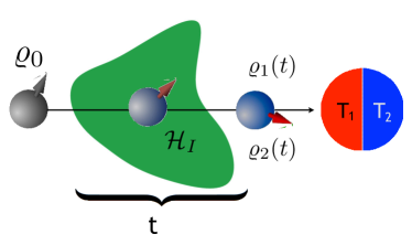
Figure 1: Discrimination of temperatures by quantum probes. A quantum system prepared in a known state $\varrho_{0}$ is let to interact with a thermal bath for a time $t$ and then measured in order to discriminate whether the state is $\varrho_{1}(t)$ or $\varrho_{2}(t)$, i.e. to infer whether the temperature of the bath is $T_{1}$ or $T_{2}$. After choosing a suitable interaction Hamiltonian ${\cal H}_{I}$, the scheme may be optimized over the initial preparation of the probe, and the value of the interaction time $t$.

In this framework, a single qubit has been suggested Jevtic et al. (2015) as an out-of-equilibrium probe to discriminate two thermal baths and, more recently, the discrimination between baths with different temperatures or statistical properties has been addressed Gianani et al. (2020), assuming that the quantum probe undergoes Markovian dynamics. In this paper, we extend these studies to more general quantum probes and taking into account the spectral structure of the bath. In particular, we assume a dephasing interaction between the probe and the bath, and derive the exact reduced evolution of the quantum probe. Then, we study the discrimination performance of our scheme for different kinds of Ohmic-like environments and for different quantum probes. In order to provide a benchmark, we first analyze discrimination by quantum probes at equilibrium, and then address the out-of-equilibrium case, looking for the optimal interaction time, leading to the smallest error probability. Our results clearly indicate that dephasing quantum probes are useful in discriminating low values of temperature, and that lower probabilities of error are achieved for intermediate values of the evolution time, i.e. for out-of-equilibrium quantum probes Razavian and Paris (2019).

The paper is structured as follows. In the next Section, we review some elements of quantum discrimination theory and establish notation. In Section III, we analyze discrimination of thermal baths by quantum probes at equilibrium. Besides being of interest in their own, the results of this Section serve as a benchmark to assess the performance of out-of-equilibrium quantum probes, which are analyzed in details in Section IV. Section V closes the paper with some concluding remarks, whereas few more details about the reduced dynamics of the quantum probes are reported in the Appendix.

II The quantum discrimination problem

In several problems of interest in quantum technology, an observer should discriminate between two or more quantum states. However, quantum states are not observable and this operation cannot be carried out directly. Furthermore, distinct states may have finite overlap, and there is no way to distinguish them with certainty Chefles (2000). The main consequence is that a correct discrimination among a generic set of quantum states is not always possible, and an intrinsic error in the process occurs. Many strategies for optimal discrimination of quantum stateBergou et al. (2004); Barnett and Croke (2009); Bae and Kwek (2015) have been suggested, each of them tailored to specific purpose. In this paper, we are going to use the minimum error discrimination strategy, which we briefly review in the following.

Let us consider the problem of binary discrimination between two quantum states $\rho_{1}$ and $\rho_{2}$ which are known in advance and occur with an priori probability $\{z_{k}\}$, $k=1,2$. Given a probability operator-valued measure (POVM) $\{\Pi_{1},\Pi_{2}\}$, the quantity $\hbox{Tr}\left[\Pi_{j}\rho_{j}\right]$ represents the probability of correctly infer the state $\rho_{j}$ by implementing the POVM. In order to optimize the discrimination, the POVM must be chosen to minimize the overall probability of error, i.e.

$$p_{e}=1-\sum_{j=1}^{2}z_{j}\hbox{Tr}\left[\Pi_{j}\rho_{j}\right],$$ (1)

Since $z_{1}+z_{2}=1$ and $\Pi_{1}+\Pi_{2}=\mathbb{I}$, $p_{e}$ may be rewritten as $p_{e}=p_{1}+\hbox{Tr}\left[\Lambda\Pi_{1}\right]=p_{2}-\hbox{Tr}\left[\Lambda\Pi_{2}\right]$ where the Hermitian operator $\Lambda$ is defined as

$$\Lambda=z_{2}\rho_{2}-z_{1}\rho_{2}.$$ (2)

Using the spectral decomposition $\Lambda=\sum_{k}\lambda_{k}|\psi_{k}\rangle\langle\psi_{k}|$, the minimum probability of error may be written in terms of the so-called Helstrom bound Helstrom (1969); Bergou (2007)

$$p_{e}=\frac{1}{2}\left(1-\sum_{k}|\lambda_{k}|\right)=\frac{1}{2}\left(1-\hbox{Tr}\left[|\Lambda|\right]\right).$$ (3)

Using the distance norm Nielsen and Chuang (2002) we can interpret the result from a geometrical point of view. Since $\hbox{Tr}\left[|\Lambda|\right]=\hbox{Tr}\left[|z_{2}\rho_{2}-z_{1}\rho_{1}|\right]=\|z_{2}\rho_{2}-z_{1}\rho_{1}\|_{1}$, if the occurrence probabilities of $\rho_{1}$ and $\rho_{2}$ are the same, we obtain

$$p_{e}=\frac{1}{2}\left[1-D(\rho_{1},\rho_{2})\right]\,,$$ (4)

where $D(\rho_{1},\rho_{2})=\frac{1}{2}\|\rho_{2}-\rho_{1}\|_{1}$ is the trace distance. This result confirms our intuition that the less two states are distant, the larger is the probability of error in discriminating them. We also remind that the optimal POVM, for which the probability of error is minimized, is given in terms of the eigenprojectors of the operator $\Lambda$, as $\Pi_{0}=\sum_{\lambda_{k}\leq 0}|\psi_{k}\rangle\langle\psi_{k}|$

III Quantum probes at thermal equilibrium

Let us now turn to the main problem of the paper, i.e. to discriminate whether a thermal bath is at temperatures $T_{1}$ or $T_{2}$ by performing measurements on a quantum probe interacting with it. In this Section, we assume that the probe is at the equilibrium with the bath. We do not study how the probe reaches the equilibrium with the bath, and simply assume that after enough time the probe has reached such equilibrium. In the next Section, we devote attention to the out-of-equilibrium case and will introduce an interaction model.

Let us consider quantum system governed by a bounded Hamiltonian $\mathcal{H}$ with an energy spectrum $\{|e_{n}\rangle,E_{n}\}_{n=0}^{N-1}$, then the equilibrium state of the probe is given by the Gibbs state

$$\rho_{eq}(\beta)=\frac{1}{Z(\beta)}\sum_{n=0}^{N-1}e^{-\beta E_{n}}|e_{n}\rangle\langle e_{n}|$$ (5)

where $Z(\beta)$ is the partition function $Z(\beta)=\sum_{n}e^{-\beta E_{n}}$ and $\beta=1/T$ (we set the Boltzmann constant to $1$ throughout the paper) is the inverse temperature of the heath bath.

Consider now the situation where we do not know in advance the temperature of the bath, but we know it must be $T_{1}$ or $T_{2}$. As a result, the thermal state will be different and our goal is to discuss the minimum probability of error in discriminating the two states $\rho_{eq}(\beta_{1})$ and $\rho_{eq}(\beta_{2})$. From the previous Section, we know that the best measurement is given by the operator $\Lambda$ in (2). In our case, since both states are diagonal in the energy eigenbasis of $\mathcal{H}$, the optimal measurement is an energy measurement. The probability of error in the discrimination is given by (4), that is

$$p_{e}^{eq}(\beta_{1},\beta_{2})=\frac{1}{2}-\frac{1}{4}\sum_{n=0}^{N-1}\left|\frac{e^{-\beta_{1}E_{n}}}{Z(\beta_{1})}-\frac{e^{-\beta_{2}E_{n}}}{Z(\beta_{2})}\right|.$$ (6)

When one of the temperature is vanishing, say $T_{2}=0$ ($\beta_{2}=+\infty$), the corresponding thermal probe collapses into the ground state $|e_{0}\rangle\langle e_{0}|$ and the probability of error becomes

$$p_{e}^{eq}(\beta_{1},+\infty) =\frac{1}{2}-\frac{1}{4}\left(\left|\frac{e^{-\beta_{1}E_{0}}}{Z(\beta_{1})}-1\right|+\sum_{n=1}^{N-1}\left|\frac{e^{-\beta_{1}E_{n}}}{Z(\beta_{1})}\right|\right)$$

$$=\frac{1}{2}\frac{e^{-\beta_{1}E_{0}}}{Z(\beta_{1})}$$ (7)

In the opposite limit, i.e. when on of the two baths has a very large temperature, say $T_{2}$ is very large ($\beta_{2}\to 0$) compared to the largest energy eigenvalue $\max_{n}\{E_{n}\}$, the corresponding thermal state approaches the equiprobable diagonal state $\rho_{eq}(0)=\mathbb{I}/N$.

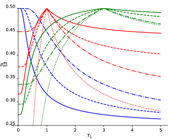
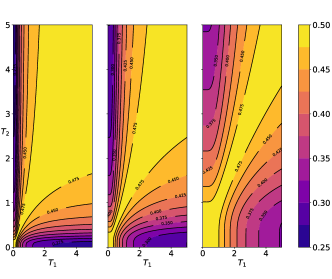
Figure 2: Upper panel: the probability of error at equilibrium $p_{e}^{eq}(T_{1},T_{2})$ for a qubit probe (11) as a function of $T_{1}$ and for different values of $T_{2}$ and $\omega_{0}$. Blue line $T_{2}=0$; Red line $T_{2}=1$; Green line $T_{2}=5$. Thick Line $\omega_{0}=\log(3)/2$, Dashed Line $\omega_{0}=\log(3)$, DotDashed Line $\omega_{0}=2\log(3)$. Lighter Red (Green) is the approximated probability of error (10) with $T_{2}=1$ ($T_{2}=5$) and $\omega_{0}=\log(3)$. Lower panels: Contour plots of $p_{e}^{eq}$ as a function of $T_{1}$ and $T_{2}$. Left: $\omega_{0}=\log(3)/2$; middle: $\omega_{0}=\log(3)$; right: $\omega_{0}=2\log(3)$.

In this limit, the partition function, up to terms $O(\beta^{2})$, may be written as

$$Z(\beta) \simeq\sum_{n=0}^{N-1}\left(1-\beta E_{n}\right)=N\left(1-\beta\bar{E}\right)\,,$$ (8)

with $\bar{E}=\sum_{n=0}^{N-1}E_{n}/N$. The Boltzmann weight becomes

$$\frac{e^{-\beta E_{n}}}{Z(\beta)}\simeq\frac{1}{N}-\frac{\beta}{N}\left(E_{n}-\bar{E}\right)\,,$$ (9)

and the probability of error is given by

$$p_{e}^{eq}(\beta_{1}, \beta_{2})=\frac{1}{2}\left(1-\frac{1}{2N}\sum_{n=0}^{N-1}\left|\left(E_{n}-\bar{E}\right)\left(\beta_{1}-\beta_{2}\right)\right|\right)$$ (10)

For a two-dimensional (qubit) probe $d=2$, a closed formula for (6) may be easily evaluated, obtaining

$$p_{e}^{eq} (\beta_{1},\beta_{2})=\frac{1}{2}\left[1+\left|\tanh\left(\frac{\omega_{0}\beta_{2}}{2}\right)-\tanh\left(\frac{\omega_{0}\beta_{1}}{2}\right)\right|\right]\,.$$ (11)

We will use this expression in the following Section, to compare performance of probes at equilibrium with that of out-of-equilibrium ones.

In the upper panel of Fig. 2, we show $p_{e}^{eq}(T_{1},T_{2})$ as a function of $T_{1}$ for a qubit system with frequency $\omega_{0}$, ($E_{0}=-\omega_{0}/2$ and $E_{1}=\omega_{0}/2$) and for different values of $T_{2}$. We see that the minimum of $p_{e}^{eq}(T_{1},T_{2})$ depends on the relative choice of $T_{1}$ and $T_{2}$. If $T_{2}=0$, the minimum is reached asymptotically for $T_{1}\to+\infty$, and we know from previous considerations that the limiting values is equal to $1/4$. Instead, for $T_{2}>0$, we have two cases: if $T_{2}\leq\omega_{0}\log(3)$, the minimum of $p_{e}^{eq}(T_{1},T_{2})$ is reached for $T_{1}\to 0$, while if $T_{2}\geq\omega_{0}/\log(3)$ then the minimum of $p_{e}^{eq}(T_{1},T_{2})$ is again obtained asymptotically for $T_{1}\to+\infty$. In the lower panels of Fig. 2, we show $p_{e}^{eq}(T_{1},T_{2})$ for the same qubit system as a function of $T_{1}$ and $T_{2}$ and for different values of $\omega_{0}$. We may clearly see the symmetry between $T_{1}$ and $T_{2}$. We also notice that as $\omega_{0}$ grows, discrimination improves, especially in the high temperature regime. This can be understood from (10), since for larger $\omega_{0}$ the second term, which is proportional to $\omega_{0}$ in the qubit case, is larger and thus $p_{e}^{eq}(T_{1},T_{2})$ is smaller.

IV Out-of-equilibrium dephasing quantum probes

Let us now study how dephasing, out-of-equilibrium, quantum probes may be exploited in the temperature discrimination problem. Here, the quantum probe is an open quantum system $S$ which effectively interacts with the reservoir, which is a thermal bath at temperature $T_{1}$ or $T_{2}$. We assume that the total Hamiltonian of the system is $\mathcal{H}=\mathcal{H}_{0}^{S}+\mathcal{H}_{0}^{B}+\mathcal{H}_{I}$, where the first term determines the free evolution of the system, the second the free evolution of the bath and the latter the interaction between the open quantum system and the reservoir. Before specifying the interaction model,let us discuss some general results about temperature discrimination, regardless of the system and of the interaction.

To perform our discrimination task, we prepare our quantum probe in a certain state and then we let it interact with the bath. We assume that the bath is at equilibrium in a Gibbs state

$$\nu_{k}=\frac{e^{-\beta_{k}\mathcal{H}_{0}^{B}}}{Z(\beta_{k})}.$$ (12)

where $\beta_{k},k=1,2$ are two distinct inverse temperature. Once fixed the probe state $\rho_{S}\equiv\rho_{S}(0)$ at time $t=0$ and the environment state $\nu_{k}$, the evolution of the initially factorized total system $\rho_{S}\otimes\nu_{k}$ is determined by a completely-positive trace-preserving (CPT) map $\Phi^{k}_{t}$. The state of the system at time $t$ will be

$$\rho_{Sk}(t)=\Phi^{k}_{t}[\rho_{S}]=\hbox{Tr}_{E}\left[U(t)\,\rho_{S}\otimes\nu_{k}\,U^{\dagger}(t)\right].$$ (13)

The two baths at different temperature define two different CPT maps, and we are going to see that the distance between these two different maps, defined in the last equation, has an upper bound which do not depend on the nature of the probe. The probability of incorrectly discriminate the two states originating from the interaction with the two baths is (4), and it depends on the trace distance $D(\rho_{S1}(t),\rho_{S2}(t))$. Since the trace distance is contractive under the action of trace-preverving map, and invariant under unitary transformations, Nielsen and Chuang (2002); Breuer et al. (2016), we have

$$D(\rho_{S1}(t),\rho_{S2}(t)) =D\Big{(}\Phi^{1}_{t}[\rho_{S}],\Phi^{2}_{t}[\rho_{S}]\Big{)}$$

$$\leq D(\rho_{S}\otimes\nu_{1},\rho_{S}\otimes\nu_{2})$$

$$=D(\nu_{1},\nu_{2})\,,$$ (14)

where the last equality is due to the fact that the state of quantum probe at time $t=0$ is fixed, regardless of the temperature, and thanks to the additivity under tensor products of the trace distance. This is an upper bound on the maximum distance between two states evolving under the same reduced dynamics with two baths at $T_{1}$ and $T_{2}$. Moreover, this bound depends only on the nature of the bath (namely its Hamiltonian $\mathcal{H}_{0}^{B}$) and on the temperatures to be discriminated. The upper bound translates into a lower bound on the probability of error (4), that is

$$p_{e}^{neq}(T_{1},T_{2})\geq\frac{1}{2}\left[1-D(\nu_{1},\nu_{2})\right]\,.$$ (15)

This bounds may be useful in dealing with finite size environment, whereas in the thermodynamical limit the orthogonality catastrophe is likely to make it useless Zanardi et al. (2008); Tonielli et al. (2019).

IV.1 Dephasing model

In this section we introduce a (pure) dephasing model that regulate the probe-environment interaction by generalizing the qubit model studied in Breuer et al. (2002). The full dynamics is generated by the Hamiltonian

$$\mathcal{H}_{T}=\mathcal{H}_{0}+\mathcal{H}_{I},$$ (16)

where $\mathcal{H}_{0}=\mathcal{H}_{0}^{S}+\mathcal{H}_{0}^{B}$ determines the free evolution of the probe and the bath, whereas $\mathcal{H}_{I}$ describes the interaction. Since we are going to consider quantum probes with a discrete energy spectrum, we may introduce an energy scale $\omega_{0}$to write the energy levels as $E_{n}=\delta_{n}\omega_{0}/2$. The Hamiltonian may be written as

$$\mathcal{H}_{0}^{S}=\frac{\omega_{0}}{2}\sum_{n=0}^{N-1}\delta_{n}|e_{n}\rangle\langle e_{n}|=\frac{\omega_{0}}{2}\mathcal{H}^{(n)}.$$ (17)

The diagonal matrix $\mathcal{H}^{(n)}$ represents the spacing of the energy levels, and it may describe the spectrum of a $n$-level system, such as qubit $\mathcal{H}^{(2)}=\sigma_{3}$, as well as that of a quantum register of 2 qubits $\mathcal{H}^{(2,2)}=\left(\sigma_{3}\otimes\mathbb{I}_{2}+\mathbb{I}_{2}\otimes\sigma_{3}\right)$Reina et al. (2002). In the second case, the spectrum might be degenerate. Moreover, where appropriate, we understand the index $n$ as a multiindex $n=(n_{1},n_{2})$, with each $n_{1}$,$n_{2}$ associated respectively with the first qubit and the second qubit.

The reservoir is described by a bath of harmonic oscillator $\mathcal{H}^{B}_{0}=\sum_{k}\omega_{k}b^{\dagger}_{k}b_{k}$, where $\omega_{k}$ are the frequencies of the $k$-th bosonic modes. Then, the interaction between the system and the reservoir is given by

$$\mathcal{H}_{I}=\mathcal{H}^{(n)}\otimes\sum_{k}(g_{k}b^{\dagger}_{k}+g^{*}_{k}b_{k})$$ (18)

The quantities $g_{k}$ are the coupling constants between each energy levels and the $k$-th mode of the bath. We assume they do not depend on the energy level with which they interact. This is justified by the assumption that the system is small compared to the size of the reservoir and a collective interaction is a good approximation. In other words, all the energy levels feel the same local environment. Moreover, we assume that in the case of quantum register, all the qubits interact locally with the same thermal bath Gebbia et al. (2020).

The model here is exactly solvable. The evolution of the quantum probe in the interaction picture, given the overall system prepared initially in a factorized state $\rho_{S}\otimes\nu$, is given by

$$\Phi^{\beta}_{t}[\rho]=\mathcal{V}^{\beta}(t)\circ\mathcal{R}(t)\circ\rho_{S}$$ (19)

where the $\circ$ is the Hadamard (entrywise) product and the quantities $\mathcal{V}^{\beta}$ and $\mathcal{R}(t)$ are given by

$$\mathcal{V}^{\beta}(t)=\sum_{j,k=0}^{N-1}e^{\frac{(\delta_{j}-\delta_{k})^{2}}{4}\Gamma(t|\beta)}|e_{j}\rangle\langle e_{k}|,$$ (20)

$$\mathcal{R}(t)=\sum_{j,k=0}^{N-1}e^{i\xi(t)\frac{\delta_{j}^{2}-\delta_{k}^{2}}{4}}|e_{j}\rangle\langle e_{k}|.$$ (21)

The evolution for a generic quantum probe, initialized in the state $\rho_{S}=\sum_{jk}\rho_{jk}|e_{j}\rangle\langle e_{k}|$ is given by

$$\rho_{S\beta}(t)=\sum_{jk}\rho_{jk}\,e^{i\xi(t)\frac{\delta_{j}^{2}-\delta_{k}^{2}}{4}}\,e^{\frac{(\delta_{j}-\delta_{k})^{2}}{4}\Gamma(t|\beta)}\,|e_{j}\rangle\langle e_{k}|.$$ (22)

The functions $\Gamma(t|\beta)$ and $\xi(t)$ are defined as follows

$$\Gamma(t|\beta) =-\sum_{k}4\frac{|g_{k}|^{2}}{\omega_{k}^{2}}\left[1-\cos(\omega_{k}t)\right]\coth\left(\frac{\omega_{k}\beta}{2}\right)$$ (23)

$$\xi(t) =-4\sum_{k}\frac{|g_{k}|^{2}}{\omega_{k}^{2}}\left[\omega_{k}t-\sin\left(\omega_{k}t\right)\right]$$ (24)

The first is the decoherence function. It represents the rate of the damping due to the interaction and it depends directly on the temperature. The second one is a temperature independent phase function which does not affect the probability of error, since the Hadamard product is distributive.

As final step, we take the continuous limit for the frequency of the bosonic bath, i.e. $\sum_{k}\to\int d\omega f(\omega)$ and $|g_{k}|^{2}\to|g(\omega)|^{2}$, where $f(\omega)$ the density of states. Upon definin the spectral density as $J(\omega)=4f(\omega)|g(\omega)|^{2}$, the decoherence function (23) and the temperature-independent phase function (24) become respectively

$$\Gamma(t|\beta) =-\int^{+\infty}_{0}\!\!\!d\omega\,J(\omega)\coth\left(\frac{\omega\beta}{2}\right)\frac{1-\cos(\omega t)}{\omega^{2}}$$ (25)

$$\xi(t) =-\int_{0}^{+\infty}\!\!\!\!d\omega\,J(\omega)\,\frac{\omega t-\sin(\omega t)}{\omega^{2}}$$ (26)

In the following, we consider environments characterized by Ohmic-like spectral densities of the form

$$J_{s}(\omega,\omega_{c})=\omega_{c}\left(\frac{\omega}{\omega_{c}}\right)^{s}\exp\left(-\frac{\omega}{\omega_{c}}\right).$$ (27)

where $\omega_{c}$ is the cutoff frequency and $s$ is the ohmicity parameter. The cutoff frequency is related to the environmental correlation time, and in turn to the decoherence time, whereas $s$ sets out the behavior of the spectral density in the low frequency range. Three main classes may be identified: the sub Ohmic ($0<s<1$), the Ohmic ($s=1$) and the superOhmic ($s>1$)Leggett et al. (1987); Shnirman et al. (2002).

Notice that for a dephasing quantum probe the populations of the energy levels are not changed by the evolution, which affects only the off diagonal terms of the density matrix of the system. In other words, there is no exchange of energy between the probe and the system under investigation, and the state of the probe is always out-of-equilibrium.

IV.2 Out-of-equilibrium qubit probe

Let us first consider a qubit probe. In this case, $\delta_{0}=-1$ and $\delta_{1}=+1$ and we make the identification $|e_{0}\rangle\to|0\rangle$ and $|e_{1}\rangle\to|1\rangle$. Thus $\mathcal{R}(t)=\mathbb{I}_{2}$ and we can write the density matrix (22) directly in the basis $|i\rangle$ at time $t$, obtaining

$$\rho^{\beta}_{S}(t)=\begin{bmatrix}1&e^{\Gamma(t|\beta)}\\ e^{\Gamma(t|\beta)}&1\end{bmatrix}\circ\rho_{S}$$ (28)

We assume no a priori information about the two temperatures to be discriminated, i.e. $z_{1}=z_{2}=\frac{1}{2}$. The operator $\Lambda$ in Eq. (2) may be written as

$$\Lambda=\begin{pmatrix}0&\rho_{10}\\ \rho_{01}&0\end{pmatrix}\,\frac{e^{\Gamma(t|\beta_{1})}-e^{\Gamma(t|\beta_{2})}}{2}$$ (29)

where $\rho_{10}$ and $\rho_{01}$ are the off diagonal elements of the initial state of the probe. The probability of error is thus given by

$$p_{e}^{neq}(\beta_{1},\beta_{2})=\frac{1}{2}\left[1-\Big{|}\rho_{10}\left(e^{\Gamma(t|\beta_{1})}-e^{\Gamma(t|\beta_{2})}\right)\Big{|}\right]$$ (30)

We notice that the probability of error depends only on the off diagonal values of the density matrix at time $t=0$ and it does not depend on the value of $\omega_{0}$. Using the Bloch vector formalism, it can be seen that the best preparation is given for $|\rho_{10}|=1/2$ and $\rho_{00}=\rho_{11}=1/2$. If $\rho_{01}$ is real, the optimal probe state is the maximally coherent state $|\psi_{S}(0)\rangle=1/\sqrt{2}\left(|0\rangle+|1\rangle\right)$.

Generally speaking, we can exactly find the optimal POVM to be implemented on the probe, which is identified by the projectors of the $\Lambda$ operator (29). Indeed, if we write $\rho_{01}=re^{-i\alpha}$, then we can write the projective measurement in terms of Pauli matrices as

$$\Pi_{1}=\frac{1}{2}\left(\mathbb{I}+\cos(\alpha)\sigma_{x}+\sin(\alpha)\sigma_{y}\right)$$ (31)

$$\Pi_{2}=\frac{1}{2}\left(\mathbb{I}-\cos(\alpha)\sigma_{x}-\sin(\alpha)\sigma_{y}\right)$$ (32)

This is a feasible POVM which depends on the initial preparation but not on the two temperatures (it does, however, depends on time since the above expression is in the interaction picture).

The above results may be interpreted in terms of coherence of the probe, i.e. the quantity $\mathcal{C}(\rho)=\sum_{i\neq j}|\rho_{ij}|$. For the state in Eq. (28), the coherence is

$$\mathcal{C}(\beta,t)=2|\rho^{0}_{01}|e^{\Gamma(t|\beta)}\,,$$ (33)

and the probability of error may be written as a function of the coherence only

$$p_{e}^{neq}(\beta_{1},\beta_{2})=\frac{1}{2}\left(1-\Big{|}\mathcal{C}(\beta_{1},t)-\mathcal{C}(\beta_{2},t)\Big{|}\right)$$ (34)

Better discrimination is thus obtained for states with larger differences of their coherence. In turn, maximally coherent states are optimal states, since they are more sensible to decoherence, which is the sole effect of the pure dephasing model.

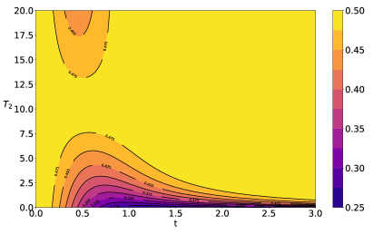
Figure 3: Probability of error $p_{e}^{neq}(T_{1},T_{2})$ using a dephasing probe, see Eq. (30), as a function of time $t$ and temperature $T_{2}$. We set $|\rho_{01}|=1/2$, $T_{1}=10$ and we consider an Ohmic environment $s=1$ with a cut-off frequency $\omega_{c}=1$.

In Fig. 3 we show the probability of error in Eq. (30) for an Ohmic environment with fixed $T_{1}=10$ and we see that for large $T_{2}$ it has only small deviations from the maximum error $p_{e}^{neq}=1/2$, meaning that in such regime the states are almost indistinguishable. Instead, in the low temperature regime and at intermediate time $t$ the $p_{e}^{neq}$ reaches smaller values. Similar behaviours may be observed for other values of $s$ and $\omega_{c}$. For this reason, henceforth we will focus only on low temperature regimes.

Next, in Fig. 4, we illustrate how the probability of error depends on the ohmicity parameter $s$ and the cut-off frequency $\omega_{c}$. There, we choose three paradigmatic values of $s$ to cover the three Ohmic regimes, that is $s=0.5$, $s=1$, and $s=3$. These plots show that a better discrimination is achievable for smaller values of the cutoff frequency and in subOhmic environments. This was predictable since in superOhmic environments the dephasing effects are smaller and consequently also the differences in the coherences are smaller, see (34). In all the plots, we may observe a common behaviour of the the probability of error: at $t=0$ $p_{e}^{neq}(T_{1},T_{2})$ is maximum and then starts to decrease (the exact behaviour depending on the nature of the environment) achieving the minimum probability of error. After the minimum, there is a slow increase which asymptotically tends the maximum error $p_{e}^{neq}$ again. This can be understood by the fact that after a large time, the decoherence effects are nearly the same for any values of temperatures $T_{1}$ and $T_{2}$.

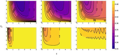
Figure 4: Plot of $p_{e}^{neq}(T_{1},T_{2})$ for a qubit system as a function of time $t$ and of $T_{2}$ with fixed $T_{1}=0$. We also set $|\rho_{01}|=1/2$. First row: $\omega_{c}=1/5$; second row: $\omega_{c}=5$. First Column $s=0.5$ (subOhmic); second column $s=1$ (Ohmic); third column $s=3$ (superOhmic).

Finally, in Fig. 5, we compare the performance of the equilibrium probe studied in Section III to those of a dephasing one. In order to have a faithful comparison, we introduce a gain factor defined as

$$\eta(T_{1},T_{2})=1-\frac{p_{e}^{neq}(T_{1},T_{2})}{p_{e}^{eq}(T_{1},T_{2})}.$$ (35)

A positive value of $\eta(T_{1},T_{2})$ means that the probability of error in the non-equilibrium regime is lower than the probability of error in the equilibrium regime. Thus $\eta$ quantifies the gain we obtain with a non equilibrium probe. On the contrary, negative $\eta$ means that an equilibrium probe provide a lower probability of error, and thus the latter is preferable. We show the gain factor in Fig. 5 for $T_{1}=0$ and for different values of $s$, $\omega_{c}$ and $\omega_{0}$. As it is apparent from the first two rows of Fig. 5, for small values of $\omega_{0}$ the equilibrium probe is almost everywhere better than the dephasing one. This is strongly different from the case of $\omega_{0}=2$, illustrated in the third and fourth rows, where for small values of the cutoff frequency (first row) and especially for $s\leq 1$ there is a wide range of interaction times and temperature of where the dephasing probe has a lower probability of error. For larger value of the cutoff frequency (second row), dephasing probes are suitable for very low temperature discrimination.

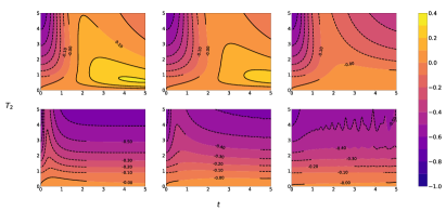
Figure 5: Plot of the gain factor $\eta(T_{1},T_{2})$ (35) as a function of time $t$ and $T_{2}$. We set $T_{1}=0$. The quantum probe is prepared in the maximally coherent state. First row: $\omega_{0}=0.5$ and $\omega_{c}=0.2$; second row: $\omega_{0}=0.5$ and $\omega_{c}=5.0$; third row: $\omega_{0}=2.0$ and $\omega_{c}=0.2$; fourth row: $\omega_{0}=2.0$ and $\omega_{c}=5.0$. First column $s=0.5$ (subOhmic); second column $s=1$ (Ohmic); third column $s=3$ (superOhmic).

IV.3 Out-of-equilibrium qutrit probe

In this section we devote our attention to a $3$-level system with equispaced energy levels. In this system, $\delta_{0}=-2$, $\delta_{1}=0$ and $\delta_{2}=+2$, and we make the identification $|e_{0}\rangle\to|0\rangle$, $|e_{1}\rangle\to|1\rangle$ and $|e_{2}\rangle\to|2\rangle$. The reduced dynamics is given by Eq. (19), with the matrix $\mathcal{V}^{\beta}(t)$ now given by

$$\mathcal{V}^{\beta}(t)=\begin{pmatrix}1&e^{\Gamma(t|\beta)}&e^{4\Gamma(t|\beta)}\\ e^{\Gamma(t|\beta)}&1&e^{\Gamma(t|\beta)}\\ e^{4\Gamma(t|\beta)}&e^{\Gamma(t|\beta)}&1\end{pmatrix}$$ (36)

In order to compare results with those obtained with a qubit probe, we consider qutrit initially prepared in a maximally coherent state $|\varphi_{3}\rangle=(|0\rangle+|1\rangle+|2\rangle)/\sqrt{3}$ and in a qubit-like state $|\varphi_{3}\rangle=(|0\rangle+|2\rangle)/\sqrt{2}$.

In the first case, the trace of the operator $|\Lambda|$ defined in (2) is given by

$$\hbox{Tr}\left[|\Lambda|\right]= \frac{1}{6}\left|e^{4\Gamma(t|\beta_{1})}-e^{4\Gamma(t|\beta_{2})}\right|$$ (37)

$$\times\left[1+\sqrt{1+8\left(\frac{e^{\Gamma(t|\beta_{1})}-e^{\Gamma(t|\beta_{2})}}{e^{4\Gamma(t|\beta_{1})}-e^{4\Gamma(t|\beta_{2})}}\right)^{2}}\right]$$

and the corresponding probability of error $p_{e3}^{neq}(T_{1},T_{2})$ may be then obtained from Eq. (3). For the state $|\varphi_{q}\rangle$, $p_{e2}^{neq}$ is instead similar to that of the qubit, i.e.

$$p_{e2}^{neq}(\beta_{1},\beta_{2})=\frac{1}{2}-\frac{|\rho_{10}|}{2}\Big{|}e^{4\Gamma(t|\beta_{1})}-e^{4\Gamma(t|\beta_{2})}\Big{|}\,,$$ (38)

with the difference that the exponentials have a more rapid decrease. The behaviour is thus similar to that of the qubit, but the minimum is achieved at smaller times.

We compare now the different probes. At first, we compare the probability of error obtained with an equilibrium probe to that obtained for a qutrit initially prepared in a maximally coherent state. The gain factor is defined as

$$\eta_{3}(T_{1},T_{2})=1-\frac{p_{e3}^{neq}(T_{1},T_{2})}{p_{e3}^{eq}(T_{1},T_{2})}\,,$$ (39)

and the value for $T_{1}=0$ in shown in the upper panel of Fig. 6. We see a positive gain factor for intermediate values of the interaction time low values of $T_{2}$.

We then compare the performance of a qutrit prepared in the state $|\varphi_{2}\rangle$ with that of a maximally coherent qubit by means the gain factor

$$\eta_{2}(T_{1},T_{2})=1-\frac{\tilde{p}_{e2}^{neq}(T_{1},T_{2})}{p_{e}^{neq}(T_{1},T_{2})}\,,$$ (40)

where $p_{e}^{neq}(T_{1},T_{2})$ is given in Eq. (30). We show $\eta_{2}(0,T_{2})$ in the middle panel of 6. We see that for short interaction times the qutrit state has always a lower probability of error for all temperatures $T_{2}$. Moreover, the lower is $T_{2}$ the larger is the time for which $\eta>0$.

Finally, we compare the probabilities of error obtained with a maximally coherent qubit and a maximally coherent qutrit. The corresponding gain factor is defined as

$$\eta_{c}(T_{1},T_{2})=1-\frac{p_{e3}^{neq}(T_{1},T_{2})}{p_{e}^{neq}(T_{1},T_{2})}$$ (41)

and it is shown in the lower panel of Fig. 6. We see that the gain factor is always positive. However, the largest improvement is achievable in the early phase of the interaction and for larger values of $T_{2}$. We thus conclude that a qutrit probe allows one to achiee lower error probability using a shorter interaction time. Upon comparing the different panels of Fig. 6 we see that preparing the qutrit in the initial state $|\varphi_{2}\rangle$ is suitable to discriminate low temperatures, whereas the maximally coherent preparation may be better employed when the two temperatures are more different.

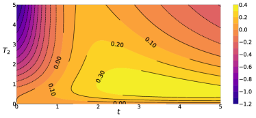
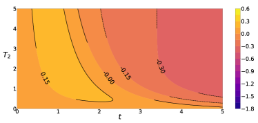
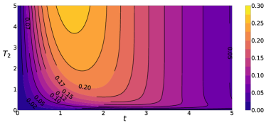
Figure 6: Upper panel: the gain factor $\eta_{3}(0,T_{2})$ of Eq. (39) as a function of the interaction time anof $T_{2}$. Middle panel: the gain factor $\eta_{2}(0,T_{2})$ of Eq.(40). Lower panel: the gain factor $\eta_{c}(0,T_{2})$ defined in Eq.(41). We have set $s=0.5$, $\omega_{c}=0.2$, $\omega_{0}=2$.

IV.4 Out-of-equilibrium quantum register made of two qubits

Finally, we investigate the performance of a quantum register of two qubits interacting locally with the thermal bath Gebbia et al. (2020); Reina et al. (2002). In this case the matrix of the levels spacing is given by

$$\mathcal{H}^{(2,2)}=\left(\sigma_{3}\otimes\mathbb{I}_{2}+\mathbb{I}_{2}\otimes\sigma_{3}\right)$$ (42)

We thus obtain that $\delta_{00}=-2$, $\delta_{01}=0=\delta_{10}$ and $\delta_{11}=+2$ and make the identifications $|e_{0}\rangle\to|00\rangle$, $|e_{1}\rangle\to|01\rangle$, $|e_{2}\rangle\to|10\rangle$ and $|e_{3}\rangle\to|11\rangle$. The reduced dynamics is given by Eq. (19), with the matrix $\mathcal{V}^{\beta}(t)$ now given by

$$\mathcal{V}^{\beta}(t)=\begin{pmatrix}1&e^{\Gamma(t|\beta)}&e^{\Gamma(t|\beta)}&e^{4\Gamma(t|\beta)}\\ e^{\Gamma(t|\beta)}&1&1&e^{\Gamma(t|\beta)}\\ e^{\Gamma(t|\beta)}&1&1&e^{\Gamma(t|\beta)}\\ e^{4\Gamma(t|\beta)}&e^{\Gamma(t|\beta)}&e^{\Gamma(t|\beta)}&1\end{pmatrix}$$ (43)

For the register initially prepared in a maximally coherent state $|\varphi_{4}\rangle=\frac{1}{4}\sum_{k}|e_{k}\rangle$ we have

$$\hbox{Tr}\left[|\Lambda|\right]= \frac{1}{8}\left|e^{4\Gamma(t|\beta_{1})}-e^{4\Gamma(t|\beta_{2})}\right|$$ (44)

$$\times\left[1+\sqrt{1+16\left(\frac{e^{\Gamma(t|\beta_{1})}-e^{\Gamma(t|\beta_{2})}}{e^{4\Gamma(t|\beta_{1})}-e^{4\Gamma(t|\beta_{2})}}\right)^{2}}\right]$$

and the corresponding probability of error $p_{e4}^{neq}(T_{1},T_{2})$ may be then obtained from Eq. (3). Having at disposal two qubits, one may wonder whether entanglement may play a role in the discrimination task. We thus consider the four Bell states as possibile initial preparation of the probe register. As it may be easily seen, the states $|\Psi^{\pm}\rangle=1/\sqrt{2}(|01\rangle\pm|10\rangle)$ are useless since they are invariant under dynamics 43. Concerning the states $|\Phi^{\pm}\rangle=1/\sqrt{2}(|00\rangle\pm|11\rangle)$ the probability of error is equal to that of the qutrit (38).

In order to asses the quantum register as quantum probe we first define the gain factor

$$\eta_{4}(T_{1},T_{2})=1-\frac{p^{neq}_{e4}(T_{1},T_{2})}{p^{eq}_{e4}(T_{1},T_{2})}$$ (45)

to compare the performance of the two-qubit dephasing probe with the corresponding equlibrium one. We show $\eta_{4}(0,T_{2})$ in the upper panel of 7, where we observe a behaviou similar to the previous dephasing probes. Here, the gain factor is larger for lower values of $T_{2}$ and for intermediate times.

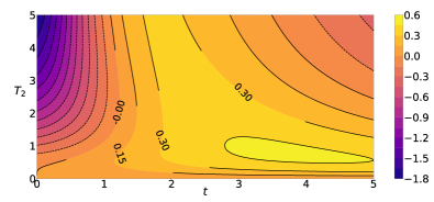
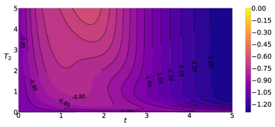
Figure 7: Upper panel: the gain factor $\eta_{4}(0,T_{2})$ defined in Eq. (45) as a function of the interaction time and $T_{2}$. Lower panel: the gain factor $\eta_{42}(0,T_{2})$ defined in Eq. (46). We set $s=0.5$, $\omega_{c}=0.2$, $\omega_{0}=2$.

It is also of interest to compare the performance of a (maximally coherent) two-qubit probe with that of a scheme using two consecutive and independent (maximally coherent) single-qubit probes. The corresponding figure of merit is given by the gain factor

$$\eta_{42}(T_{1},T_{2})=1-\frac{p^{neq}_{e4}(T_{1},T_{2})}{\left[p^{neq}_{e}(T_{1},T_{2})\right]^{2}}\,,$$ (46)

where $p_{e}^{neq}(T_{1},T_{2})$ is given in Eq. (30). As it is apparent from the lower panel of Fig. 7, there is no advantage in using two qubits simultaneously since the gain factor is always negative in the considered region.

V Conclusion

In this paper, we have analyzed in details the use of quantum probes to discriminate two structured baths at different temperatures. In particular, we have addressed quantum probes interacting with the thermal bath by a dephasing Hamiltonian and compared the discrimination performance with those of equilibrium probes.

At first, we have addressed the discrimination problem for an equilibrium probe and evaluated the probability of error in the discrimination problem, showing that energy measurement is optimal in this regime . We have then moved to out-of-equilibrium dephasing probes and derived the exact reduced dynamics for a finite quantum system locally interacting with a Ohmic-like thermal bath. Upon exploiting this result, we have studied the behaviour of the probability of error as a function of the interaction time and found that in the low-temperature regime out-of-equilibrium probes outperform equilibrium ones. For all the environments here considered there is a finite value of the interaction time minimizing the probability of error. In particular, for sub-Ohmic environments decoherence effects are stronger, and this leads to lower error probability for shorter interaction times. In turn, it results that for qubits systems, maximally coherent states represent the best preparation of the probe for the discrimination task.

We have also compared qubit probes with qutrit ones, and have shown numerically that qutrits allows one to achieve lower error probability. Finally, we have also compared schemes based on simultaneous probes (i.e. quantum registers made of two qubits) to those of based on two single-qubit probes, showing that the latter has always the lowest probability of error. Overall, our results indicate that dephasing quantum probes are useful for the taks of discriminating temperatures, and that out-of-equilibrium coherent quantum probes represent a resource not only for quantum estimation but also for quantum discrimination.