Supplementary information for Nontopological zero-bias peaks in full-shell nanowires induced by flux tunable Andreev states

Supplementary text

Model

The theoretical model used to describe the experimental results of this work is presented in what follows. It consists of a single impurity Anderson model (SIAM) coupled to a superconducting reservoir, the so-called superconducting Anderson model, in which we take into account the Little-Parks (LP) modulation of the gap with the applied flux, $\phi$ (see the details below). The impurity is also coupled to a normal reservoir, hence forming a superconductor-quantum dot-normal (SC-QD-N) junction.

The formation of the QD is taken here as an empirical fact derived from our experimental results. Its model is kept minimal, given that the precise mechanism behind its formation remains relatively unclear. Similarly, we do not add an explicit spin-orbit coupling term. Such a term would be crucial in a topological phase study, but not in the trivial regime of interest here. If the typical dot lengthscale becomes larger than the spin-orbit length (estimated in these wires to be in the hundreds of nanometers), it would modify the energy distribution and spatial profiles of the dot states, and also their couplings to the SC and N leads. As our low-energy model has a single dot orbital, any spin-orbit coupling in a more microscopic model can be understood to be already incorporated in the energy and couplings of the single dot level, which are fitting parameters in our model.

Despite its simplicity, this model correctly captures the interplay between two competing mechanisms, namely: Coulomb blockade in the QD region and Andreev processes at the superconducting interface. Each of them favors a different ground state (GS) configuration: the former favors a doublet phase, $|D\rangle$, with spin $\frac{1}{2}$, whereas the latter a singlet phase, $|S\rangle$, with spin 0.

The Hamiltonian of the system reads: $H=H_{QD}+H_{N}+H_{S}+H_{T}^{N}+H_{T}^{S}$. Here, $H_{QD}$ refers to the decoupled dot Hamiltonian given by

$$H_{QD}=\sum_{\sigma}\epsilon_{\sigma}d^{\dagger}_{\sigma}d_{\sigma}+Un_{\uparrow}n_{\downarrow},$$ (S1)

where $d_{\sigma}$ ($d_{\sigma}^{\dagger}$) destroys (creates) an electron with spin $\sigma=\{\uparrow,\downarrow\}$ and energy $\epsilon_{\sigma}=\epsilon_{0}\mp V_{Z}$, where $V_{Z}=g\mu_{B}B/2$ refers to the Zeeman energy owing to the external magnetic field $B$ (with $g$ and $\mu_{B}$ being, respectively, the gyromagnetic factor and the Bohr’s magneton). Electron-electron correlations in the dot occupations $n_{\sigma}=d^{\dagger}_{\sigma}d_{\sigma}$ are included by means of the charging energy $U$. The Hamiltonian of the normal reservoir is given by

$$H_{N}=\sum_{k_{N}\sigma}\varepsilon_{k_{N}\sigma}c^{\dagger}_{k_{N}\sigma}c_{k_{N}\sigma},$$ (S2)

where $c^{\dagger}_{k_{N}\sigma}$ ($c_{k_{N}\sigma}$) creates (destroys) an electron with momentum $k_{N}$, spin $\sigma$ and single-particle energy $\varepsilon_{k_{N}\sigma}$ in the normal reservoir.

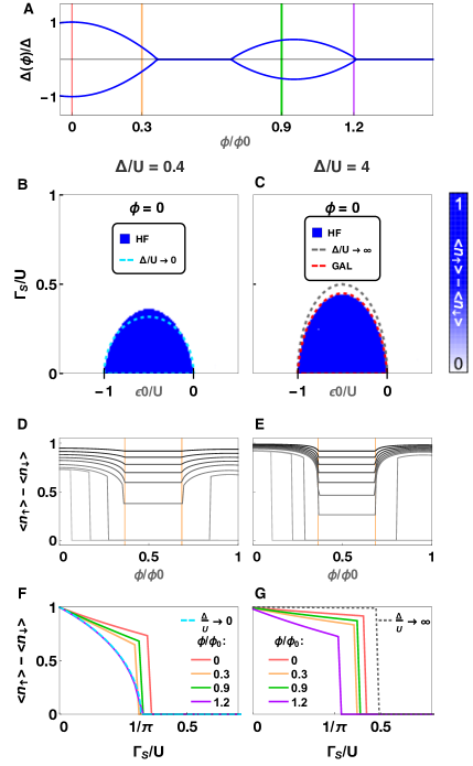
Figure S1: Gap modulation of the phase diagram through the Little-Parks effect. (A) LP modulation of the superconducting gap in the destructive regime vs normalized flux $\phi/\phi_{0}$ . (B and C) Full phase diagram of $\langle n_{\uparrow}\rangle-\langle n_{\downarrow}\rangle$ vs $\Gamma_{S}/U$ and $\epsilon_{0}/U$ for $\phi=0$ in the small and large $\Delta/U$ regimes, respectively. Only the LP effect is included here so we take $g=0$. Hartree-Fock (HF) solution: Inside the dark blue dome the superconductor-quantum dot (SC-QD) system is in a doublet ground state (GS), whereas it is in a singlet GS in the white region. Grey, red and cyan dashed lines mark the analytic boundaries in the $\Delta/U\rightarrow\infty$ (atomic), generalized atomic (GAL) and $\Delta/U\rightarrow 0$ (Anderson) approximations, respectively. (D and E) $\langle n_{\uparrow}\rangle-\langle n_{\downarrow}\rangle$ vs $\phi/\phi_{0}$ for fixed $\epsilon_{0}=-U/2$ and increasing values of $\Gamma_{S}/U$ from 0.06 (black) to 0.36 (D) and 0.45 (E) (light grey). The orange lines mark the destructive LP regime. Note that for the larger couplings, the singlet phase occurs before the LP destructive region. Similarly, the system is back to a doublet well outside the LP destructive region. (F and G) $\langle n_{\uparrow}\rangle-\langle n_{\downarrow}\rangle$ vs $\Gamma_{S}/U$ for fixed $\epsilon_{0}=-U/2$ and increasing fluxes marked with colors in (A) for the two regimes of (B) and (C), respectively, also in the absence of Zeeman effect. The LP effect results in an oscillatory modulation of the dome. Parameters: $g=0$, $\Gamma_{N}\approx 0$, $\Delta=0.2$ meV, $R=50$ nm, $d=35$ nm, and $U=0.5$ meV ($U=0.05$ meV) in (B), (D) and (F) [in (C), (E) and (G)].

Since the superconducting lead (full-shell proximitized NW) to which the dot is coupled has a doubly connected geometry and is longitudinally threaded by a magnetic flux, $\phi=\pi R^{2}B$ (with $R$ being the NW radius), the LP effect will manifest in the form of a modulation of the Bardeen–Cooper–Schrieffer (BCS) gap, $\Delta(\phi)$   (?, ?, ?). Such modulation may result in a full suppression of superconductivity in finite flux regions for cylinders characterized by small radius and thickness $d$, as compared to the zero temperature superconducting coherence length $\xi$, namely $d,R\ll\xi$  (?), which is the relevant experimental situation. Other than these finite size effects in the transversal direction, the finite length of the proximitized wire does not play a role since, in the experiment, this SC segment is effectively grounded. In the opposite case of a floating segment, a finite charging energy in the SC itself must be included, which significantly modifies the YSR picture presented here  (?, ?). Therefore, the resulting Hamiltonian for the SC is a standard BCS model that incorporates the LP modulation of the gap and reads

$$H_{S}=\sum_{k_{S}\sigma}\varepsilon_{k_{S}\sigma}c^{\dagger}_{k_{S}\sigma}c_{k_{S}\sigma}+\sum_{k_{S}}\Delta(\phi)(c^{\dagger}_{k_{S}\uparrow}c^{\dagger}_{-k_{S}\downarrow}+h.c.),$$ (S3)

where $c^{\dagger}_{k_{S}\sigma}$ ($c_{k_{S}\sigma}$) denotes the creation (destruction) operator in the superconducting lead with momentum $k_{S}$, spin $\sigma$ and energy $\varepsilon_{k_{S}\sigma}$. All energies are measured with respect to the chemical potential of the SC.

As was shown in  (?), a complete analogy can be established between pair-breaking mechanisms due to flux-induced circulating supercurrents in the shell and that of paramagnetic impurities in a disordered SC. Thus, the time-dependent Ginzburg-Landau formalism used to describe the latter can be applied to the former, giving rise to the following expression for the critical temperature $T_{C}(\phi)$ (see  (?) for a comprehensive derivation):

$$0=\ln\left(\frac{T_{C}(\phi)}{T_{C}^{0}}\right)+\psi\left(\frac{1}{2}+\frac{\Lambda_{n}(\phi)}{2\pi T_{C}({\phi})}\right)-\psi\left(\frac{1}{2}\right),$$ (S4)

where $T_{C}^{0}$ is the critical temperature at zero flux, $n$ is the fluxoid winding number, $\psi$ is the digamma function, and $\Lambda_{n}$ is the pair-breaking term corresponding to a hollow superconducting cylinder. This pair-breaking term can be derived solving the Ginzburg-Landau equations in the presence of impurities  (?), and yields

$$\Lambda_{n}(\phi)=\frac{T_{C}^{0}}{\pi}\frac{\xi^{2}}{(R+d)^{2}}\Big{[}4\left(n-\frac{\phi}{\phi_{0}}\right)^{2}+\frac{d^{2}}{(R+d)^{2}}\left(\frac{\phi^{2}}{\phi_{0}^{2}}+\left(\frac{1}{3}+\frac{d^{2}}{20(R+d)^{2}}\right)n^{2}\right)\Big{]},$$ (S5)

where $\phi_{0}$ denotes the superconducting flux quantum, $\phi_{0}=h/2e$. Once $T_{C}(\phi)$ is known, in small devices ($d,R\ll\xi$) the field-dependent critical current $I_{C}(\phi)$ can be expressed as $I_{C}(\phi)\propto T_{C}(\phi)^{3/2}$, thanks to a Ginzburg-Landau approximated relation in the presence of a magnetic field   (?). In the ballistic regime, $\Delta(\phi)$ is proportional to $I_{C}(\phi)$ and thus

$$\frac{\Delta(\phi)}{\Delta}\approx\left(\frac{T_{C}(\phi)}{T_{C}^{0}}\right)^{3/2},$$ (S6)

where $\Delta$ is the gap at $\phi=0$.

Departures from a power-law dependence of $\Delta(\phi)$ on $T_{C}(\phi)$ in the presence of pair-breaking mechanisms are predicted to happen as we go beyond the Ginzburg-Landau/BCS description  (?, ?, ?). However, Eq. (S6) suffices to accurately capture the LP modulation found in the experiment, as we describe in the Materials and Methods subsection.

The remaining two terms in the Hamiltonian:

$$H_{T}^{S}=\sum_{k_{S}\sigma}\left(V_{k_{S}}c^{\dagger}_{k_{S}\sigma}d_{\sigma}+h.c.\right),$$ (S7)

and

$$H_{T}^{N}=\sum_{k_{N}\sigma}\left(V_{k_{N}}c^{\dagger}_{k_{N}\sigma}d_{\sigma}+h.c.\right),$$ (S8)

stand for the couplings between the dot and the SC lead and the normal reservoir, respectively. These two tunneling processes define the two tunneling rates $\Gamma_{N,S}/\hbar$, where $\Gamma_{N,S}=\pi\sum_{k_{N,S}}|V_{k_{N,S}}|^{2}\delta(\omega-\epsilon_{k_{N,S}})=\pi|V_{{N,S}}|^{2}\rho_{{N,S}}$ are energy broadenings, with $\rho_{{N,S}}$ being the density of states of the normal/superconducting lead evaluated at the Fermi energy.

In order to compute spectral observables, the relevant quantity that has to be determined is the equilibrium retarded Green’s function in the dot, namely $\hat{\mathcal{G}}_{\sigma}(\omega)$. In a Nambu $2\times 2$ basis spanned by $\Psi_{\sigma}=\{d_{\sigma},d^{\dagger}_{-\sigma}\}^{T}$, the Dyson equation reads

$$\hat{\mathcal{G}}_{\sigma}^{-1}(\omega,\phi)=\hat{\mathcal{G}}_{0\sigma}^{-1}(\omega,\phi)-\hat{\Sigma}_{\sigma}(\omega,\phi).$$ (S9)

Here, $\hat{\mathcal{G}}_{0\sigma}(\omega)$ refers to the decoupled and non-interacting dot retarded Green’s function and $\hat{\Sigma}_{\sigma}=\hat{\Sigma}_{\sigma}^{QD}+\hat{\Sigma}_{\sigma}^{N}+\hat{\Sigma}_{\sigma}^{S}$ is the self-energy that takes into account the coupling to the leads, $\hat{\Sigma}_{\sigma}^{N,S}$, and the Coulomb interaction in the dot, $\hat{\Sigma}_{\sigma}^{QD}$. While a complete description of the problem needs to fully take into account electron-electron correlations, the Coulomb blockade regime is well captured by considering a diagrammatic expansion of the dot self-energy up to the lowest order in $U$:

$$\hat{\Sigma}^{QD,HF}_{\sigma}=U\begin{pmatrix}\langle n_{-\sigma}\rangle&\langle d_{\uparrow}d_{\downarrow}\rangle\\ \langle d^{\dagger}_{\downarrow}d^{\dagger}_{\uparrow}\rangle&-\langle n_{\sigma}\rangle\end{pmatrix}.$$ (S10)

This mean-field approximation, which neglects high-order correlations, is known as the Hartree-Fock-Bogoliubov (HF) approximation  (?, ?, ?). This level of approximation is enough to achieve an excellent agreement with the experimental results (away from the Kondo regime). Within this mean field picture, the retarded dot Green’s function reads

$$\hat{\mathcal{G}}_{\sigma}^{r,HF}(\omega,\phi)=\frac{1}{D(\omega,\phi)}\small{\begin{pmatrix}\omega+\epsilon_{-\sigma}+i\Gamma_{N}+\Gamma_{S}\frac{\omega}{\sqrt{\Delta(\phi)^{2}-\omega^{2}}}+U\langle n_{\sigma}\rangle&\Gamma_{S}\frac{\Delta(\phi)}{\sqrt{\Delta(\phi)^{2}-\omega^{2}}}+U\langle d_{\uparrow}d_{\downarrow}\rangle\\ \Gamma_{S}\frac{\Delta(\phi)}{\sqrt{\Delta(\phi)^{2}-\omega^{2}}}+U\langle d^{\dagger}_{\downarrow}d^{\dagger}_{\uparrow}\rangle&\omega-\epsilon_{\sigma}+i\Gamma_{N}+\Gamma_{S}\frac{\omega}{\sqrt{\Delta(\phi)^{2}-\omega^{2}}}-U\langle n_{-\sigma}\rangle\end{pmatrix},}$$ (S11)

where $D(\omega,\phi)$ is given by the determinant of $[\hat{\mathcal{G}}_{\sigma}^{r,HF}]^{-1}(\omega,\phi)$. The Andreev bound states (ABSs) are given by the zeroes of the determinant and can be written in a compact form as:

$$\left[\omega+i\Gamma_{N}+\Gamma_{S}\frac{\omega}{\sqrt{\Delta(\phi)^{2}-\omega^{2}}}\pm\tilde{V}_{Z}\right]^{2}=\tilde{\epsilon}^{2}+\left|\frac{\Gamma_{S}\Delta(\phi)}{\sqrt{\Delta(\phi)^{2}-\omega^{2}}}+\tilde{\Delta}\right|^{2},$$ (S12)

with $\tilde{V}_{Z}=V_{Z}+\frac{U}{2}(\langle n_{\uparrow}\rangle-\langle n_{\downarrow}\rangle)$, $\tilde{\epsilon}=\epsilon_{0}+\frac{U}{2}(\langle n_{\uparrow}\rangle+\langle n_{\downarrow}\rangle)$ and $\tilde{\Delta}=U\langle d_{\uparrow}d_{\downarrow}\rangle$. Physically, $\tilde{V}_{Z}$ and $\tilde{\epsilon}$ can be physically interpreted as an effective exchange field and a level shift due to correlations. When $\Delta\rightarrow 0$ they define two Coulomb resonances at $\tilde{\epsilon}\pm\tilde{V}_{Z}$ and broadened by $\Gamma_{N}+\Gamma_{S}$. When $\tilde{\epsilon}=0$, these two resonances are located at $\pm(V_{Z}+U/2)$. In the presence of superconducting correlations, these resonances become ABSs whose location and physical character depend on the ratios of different parameters [$\Delta(\phi)/U$, $\Gamma_{S}/U$, etc.] that give rise to different physical regimes, as we explain below.

The average values concerning the dot level occupations in Eqs. (S11) and (S12) are determined self-consistently in equilibrium. Once $\hat{\mathcal{G}}_{\sigma}^{r,HF}(\omega)$ is known, we can easily calculate the density of states (DOS) $\rho(\omega,\phi)=-\frac{1}{\pi}{\rm{Im\,Tr}}[\mathcal{G}_{\sigma}^{r,HF}(\omega,\phi)]$, where the trace includes both spin and Nambu degrees of freedom. At small bias voltage $V$ and temperature $T$, the differential conductance $dI/dV$ in the tunneling limit provides an approximate measure of the QD DOS at energy $eV$. The sets of parameters for each simulation in the main text are collected in Table S1.

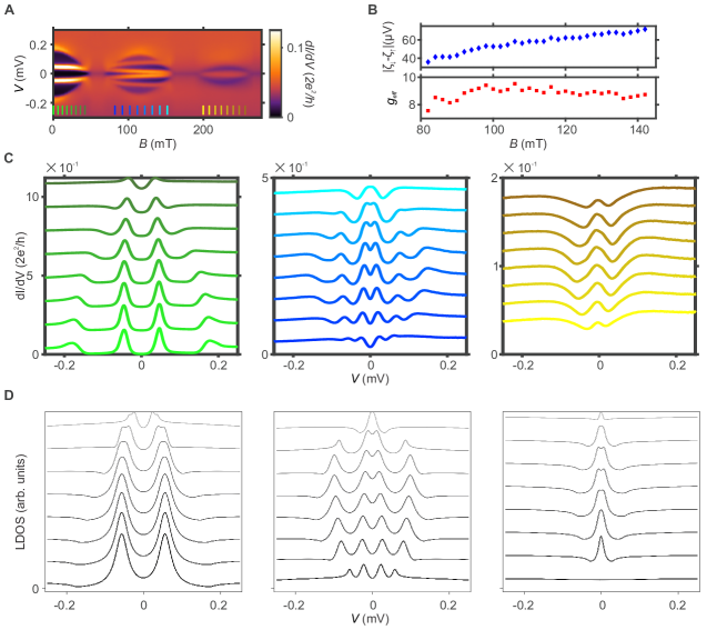
Figure S11: ZBP in the second lobe due to ABSs in device B. (A) Same plot as Fig. 4D but with coloured markers. (B) ABSs splitting in the 1L at positive bias versus $B$, (upper panel) and effective g-factor $g_{\rm{eff}}$ extracted from their splitting (lower panel). (C) Line traces extracted from (A) for the 0L, 1L and 2L (from left to right) illustrating how the ABSs merge at zero bias at the end of the 1L. The lower trace of the 0L is taken at $B=0$ and the upper one is taken at $B=42\,$\mathrm{m}\mathrm{T}$$. They are shifted by $0.3{e^{2}}/{h}$ with respect to each other. For the 1L, the line traces are shifted by 0.12 $e^{2}/{h}$ and they range from $B=82\,$\mathrm{m}\mathrm{T}$$ (lower one) to $B=152\,$\mathrm{m}\mathrm{T}$$ (upper one). Finally, for the 2L, the line traces are shifted by $0.04{e^{2}}/{h}$ and range from $B=200\,$\mathrm{m}\mathrm{T}$$ (lower one) to $B=256\,$\mathrm{m}\mathrm{T}$$ (upper one). (D) Numerical simulation of (C). The parameters can be found in Table S1.

	$U[\rm{meV}]$	$\epsilon_{0}/U$	$g$	$\Delta[\rm{meV}]$	$\Gamma_{S}/U$	$\Gamma_{S}/\Delta$	$\Gamma_{N}/\Delta$	$R$ [nm]	$d$ [nm]
Fig. 4F(left)	2.5	-0.97	13	0.18	0.036	0.5	0.07	65	25
Fig. 4F(center)	2.5	-0.95	13	0.18	0.036	0.5	0.07	65	25
Fig. 4F(right)	2.5	-0.93	13	0.18	0.036	0.5	0.07	65	25
Fig. 5, G and H	1.5	-0.93	13	0.14	0.075	0.8	0.1	64	23
Fig. S4	1.5	-0.91	14.3	0.18	0.12	1	0.16	50	35
Fig. S9D	2.5	-0.5	13	0.18	0.18	2.5	0.3	65	25
Fig. S11D	1	-0.5	13	0.18	0.33	1.83	0.22	65	25

Table S1: Parameters used in the numerical simulations of the main text. $\Delta$ values were determined from experimental evidence. $R$ and $d$ have been extracted by using them as free parameters in Eqs. (S5) and (S6) and finding the best agreement with the experimental LP data (see Materials and Methods subsection). Going from flux $\phi$ to magnetic field $B$ we assumed a circular effective section of radius $R+10\rm{nm}$ which captures the finite penetration length of $B$ in the SC shell and is required to achieve experimental agreement.

While the full solution of the zeroes in Eq. (S12) is needed to find the ABSs at arbitrary energy, one may find some useful analytic boundaries in different parameter regimes, as we discuss now.

Large $U$ approximations

The experimental regime discussed in the main text corresponds to small $\Delta(\phi)/U$ (large-$U$ limit). In this case, singlets are Yu-Shiba-Rusinov (YSR)-like superpositions between the singly occupied state in the QD and quasiparticles below the gap in the SC. The ABS position in this limit can be much lower than the original gap and, assuming that $\tilde{V}_{Z}$ is the largest scale in the problem, namely that the system is in a doublet GS, we can find the poles of Eq. (S12) as ($\Gamma_{N}=0$):

$$\omega\approx\pm\Delta(\phi)\frac{\tilde{V}^{2}_{Z}-\tilde{\Gamma}^{2}_{S}-\tilde{\epsilon}^{2}}{\sqrt{[\tilde{\Gamma}^{2}_{S}+\tilde{\epsilon}^{2}-\tilde{V}^{2}_{Z}]^{2}+4(\tilde{\Gamma}_{S}-\tilde{\Delta})^{2}\tilde{V}^{2}_{Z}}},$$ (S13)

which is a generalization of the classical expression for YSR states in a SC  (?, ?, ?, ?) (see also Ref.  (?) for a different derivation using an effective Kondo model). Note that the poles cross zero energy when  (?)

$$\tilde{V}^{2}_{Z}=\tilde{\Gamma}^{2}_{S}+\tilde{\epsilon}^{2}$$ (S14)

We note that this criterion for parity crossings of YSR states in a QD is essentially the same as the criterion for topological superconductivity and Majorana zero modes in a proximitized NW (by just substituting $\tilde{\Gamma}_{S}\rightarrow\Delta^{NW}$, $\tilde{\epsilon}\rightarrow\mu^{NW}$ and $\tilde{V}_{Z}\rightarrow V_{Z}^{NW}$  (?, ?). This is yet another example that emphasises the difficulty of making a clear distinction between parity crossings in QDs and Majorana zero modes in NWs. The connection between Eq. (S13) and the standard expression for YSR states  (?, ?, ?, ?) is evident in the limit $\tilde{\epsilon}\rightarrow 0$, $\tilde{\Delta}\rightarrow 0$, where we recover

$$\omega=\pm\Delta(\phi)\frac{1-\left(\frac{\Gamma_{S}}{\tilde{V}_{Z}}\right)^{2}}{1+\left(\frac{\Gamma_{S}}{\tilde{V}_{Z}}\right)^{2}}=\pm\Delta(\phi)\frac{1-J^{2}}{1+J^{2}}.$$ (S15)

Using $\langle n_{\uparrow}\rangle-\langle n_{\downarrow}\rangle=1$, the exchange constant is $J=2\Gamma_{S}/(U+2V_{Z})$, and we recover the standard expression with a exchange constant in a YSR/Kondo language $J=\pi jS\rho_{S}/2$, with $S=1/2$ and $j=8|V_{S}|^{2}/(U+2V_{Z})$.

Typically, $U$ can be experimentally extracted from the size of Coulomb blockade diamonds and we can use Eq. (S15) to find the value of $\Gamma_{S}$ in the doublet regime by just substituting the ABS energy position at $B=0$, namely $\omega=\pm\zeta$:

$$\Gamma_{S}=\frac{U}{2}\sqrt{\frac{(1-\zeta/\Delta)}{(1+\zeta/\Delta)}}.$$ (S16)

Using this procedure, we find a good agreement between the analytical YSR expression of Eq. (S15) and the experiments in the full magnetic field range [see Fig. 3D of the main text]. Further improvement in the agreement can be found by performing full HF numerics directly from Eq. (S12) [typically using slightly smaller $\Gamma_{S}$ values as the ones directly extracted from Eq. (S16)]. Note that the way the magnetic field enters in Eqs. (S13) and (S15) (through $\Delta(\phi)$ and $V_{Z}$) strongly deviates from a standard linear Zeeman dispersion, which explains why the ABSs in the experiments show almost no dispersion against magnetic field.

These YSR singlets eventually become Kondo singlets in the destructive LP regions when $\Delta(\phi)\rightarrow 0$. One can estimate the flux at which Kondo physics dominates over superconductivity by using the expression for the $V_{Z}=0$ Kondo temperature at the symmetry point $T_{K}\approx 0.3\sqrt{\Gamma_{S}U}e^{-\frac{\pi U}{8\Gamma_{S}}}\approx 0.2U\sqrt{J}e^{-\frac{\pi}{4J}}$. For example, using the parameters of Fig. 4(g) of the main text, we can estimate that a Kondo GS develops when $\Delta(\phi)\lesssim T_{K}\approx 0.044\;\rm{meV}\approx 0.24\Delta$, which first happens at $\phi\approx 0.35\phi_{0}$, in very good agreement with the experimental observation of a Kondo effect in the first destructive LP region at $B\approx 50$ mT. Nevertheless, we emphasise that a full calculation of the flux at which the Kondo effect develops constitutes a rather involved problem, well beyond the scope of this theoretical analysis, and should be the subject of future studies.

When approaching a singlet-doublet crossing near a charge-degeneracy point as a function of $\epsilon_{0}$, the self-consistent HF method is known to exhibit small discontinuities between non-magnetic and magnetic solutions  (?, ?). In these cases (Fig. 4E of the main text), and since these discontinuities can result in unphysical energy shifts of the ABSs near the crossing, we find the mean-field values in Eq. (S12) that provide the best agreement with the experiment.

Large $\Delta$ approximations

For completeness, we also discuss the opposite large gap limit, where the coupling to the SC $\Gamma_{S}$ mainly induces local superconducting correlations in the QD. This can be easily seen by taking the so-called $\Delta\rightarrow\infty$ atomic limit  (?, ?, ?), where superconducting singlets are just bonding and antibonding superpositions of empty and doubly-occupied states in the QD, namely $|S_{\pm}\rangle=|0\rangle\pm|2\rangle$. In this atomic limit, the singlet-doublet boundary (parity crossing) can be easily obtained by taking the $\omega\rightarrow 0$ limit in Eq. (S12) ($V_{Z}=0$ and $\Gamma_{N}=0$):

$$\left(\frac{U}{2}\right)^{2}=\Gamma_{S}^{2}+\left(\epsilon_{0}+\frac{U}{2}\right)^{2}.$$ (S17)

Expanding the determinant further to order $\omega^{2}$ allows to capture finite $\Delta$ corrections to the above atomic limit boundary. This is called the generalized atomic limit (GAL)  (?, ?), whose singlet-doublet boundary now reads

$$\frac{U^{2}}{4(1+\frac{\Gamma_{S}}{\Delta})^{2}}=\Gamma_{S}^{2}+\left(\epsilon_{0}+\frac{U}{2}\right)^{2}.$$ (S18)

It can be used to demonstrate that HF provides a very good approximate solution of the problem, particularly near the symmetry point $\epsilon_{0}=-U/2$, when neglecting the above-gap continuum contribution to the anomalous propagator. Further improvement can be reached by performing finite-$\Delta$ self-consistent perturbation theory around the atomic limit both for $V_{Z}=0$  (?) and $V_{Z}\neq 0$  (?, ?). The resulting boundaries are, however, no longer analytic.

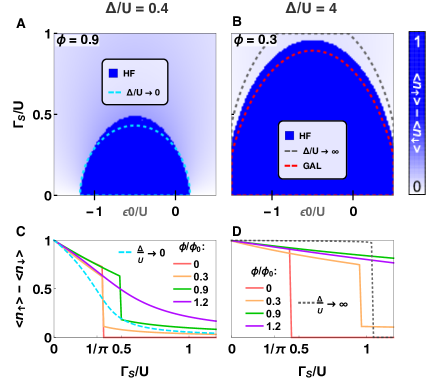
Figure S2: Gap plus Zeeman modulation of the phase diagram owing to external flux. (A and B) Full phase diagram of $\langle n_{\uparrow}\rangle-\langle n_{\downarrow}\rangle$ vs $\Gamma_{S}/U$ and $\epsilon_{0}/U$ at $\phi/\phi_{0}=0.9$ ($\phi/\phi_{0}=0.3$) in the small (large) $\Delta/U$ regime. Hartree-Fock (HF) solution: Inside the dark blue dome the SC-QD system is in a doublet ground state (GS), whereas it is in a singlet GS in the white region. Grey, red and cyan dashed lines mark the analytic boundaries in the $\Delta/U\rightarrow\infty$ (atomic), generalized atomic (GAL) and $\Delta/U\rightarrow 0$ (Anderson) approximations, respectively. (C and D) $\langle n_{\uparrow}\rangle-\langle n_{\downarrow}\rangle$ vs $\Gamma_{S}/U$ for fixed $\epsilon_{0}=-U/2$ in the small and large $\Delta/U$ regimes, respectively, and increasing fluxes marked with colors in (A). The dashed cyan line in (C) corresponds to the $B=0$, $\Delta/U\rightarrow 0$ limit, whereas the dashed grey line in (D) corresponds to the $B=0$, $\Delta/U\rightarrow\infty$ limit. In this figure, both the Zeeman effect, through a non-zero $g=11$, and the LP effect are included, the rest of parameters are chosen as those of Fig. S1. The doublet dome exhibits a non trivial evolution with the applied flux due to two different mechanisms: the Zeeman effect that expands the doublet dome in both $x$ and $y$ directions and the LP effect which leads to an oscillatory modulation.

Phase diagrams in different coupling regimes

Whether the SC-QD GS is a singlet or a doublet is revealed by the magnetic field evolution of the subgap states, with a change in GS parity whenever they cross zero energy. This in turn results from the competition of two mechanisms: LP effect that modulates the gap and the Zeeman effect that shifts the dot level energy. The first effect is illustrated in Fig. S1A, where we show the oscillatory modulation of the superconducting gap vs the applied normalized flux $\phi/\phi_{0}$. The gap exhibits the so-called destructive LP effect, whereby the gap decreases in the zeroth lobe from its maximum value at $\phi=0$, disappears in the first destructive region, reemerges in the fist lobe, and so on. In Fig. S1, B and C, we analyze the role of LP modulation of the gap on the phase diagram of the problem, disregarding for the moment the Zeeman effect (i.e., taking $g=0$). We plot the difference of spin-polarised occupations $\langle n_{\uparrow}\rangle-\langle n_{\downarrow}\rangle$ in the self-consistent HF approximation versus $\Gamma_{S}/U$ and $\epsilon_{0}/U$. Both panels show the phase diagram for the largest gap of the problem, $\Delta$ (i.e., the gap at $\phi=0$), but for different charging $U$, resulting in small, Fig. S1B, and large, Fig. S1C, $\Delta/U$ ratios. Already at this level, it it important to stress how the different ratios influence the singlet-doublet boundary. The gap evolution across LP oscillations (without Zeeman) modifies the singlet-doublet boundary most strongly at the symmetry point $\epsilon_{0}=-U/2$. This LP modulation of the boundary is clearly seen in Fig. S1, D and E, where we show how the spin polarisation varies with flux at the symmetry point $\epsilon_{0}=-U/2$ for increasing $\Gamma_{S}$ (from top to bottom curves). Both panels show that doublet-singlet-doublet transitions can be induced by LP modulation. Note that while our HF does not provide a quantitative result at doublet phases (the spin should be fully screened in this phase, $\langle n_{\uparrow}\rangle-\langle n_{\downarrow}\rangle\rightarrow 0$, owing to Kondo correlations), the overall trend is perfectly captured. These non-monotonic doublet-singlet-doublet transitions are, in turn, responsible for the phenomenology discussed in Fig. 4 of the main text. In this regime, the measured excitations in the experiments clearly show a YSR singlet-Kondo (co-tunneling) excitation-YSR singlet transition mediated by flux. Note that for the largest coupling $\Gamma_{S}$ shown in the plot, the boundaries occur well before/after the destructive LP region (delimited by orange lines). In this latter case, the singlet phase extends well beyond the destructive LP region. This could result in a Kondo effect and a singlet-doublet parity crossing in flux regions well inside the first lobe where Majoranas are also predicted. Apart from a non-monotonic dependence of the boundary on $\phi$, owing to the non-monotonic $\Delta(\phi)$, we clearly observe how the two analytic boundaries of the problem, the normal Anderson model boundary at $\Gamma_{S}/U=1/\pi$ in the $\Delta\rightarrow 0$ (cyan dashed line) and the $\Delta/U\rightarrow\infty$ boundary at $\Gamma_{S}/U=0.5$ (grey dashed line), are approached. The first limit, in particular, is approached in the destructive LP phases where the superconducting gap fully closes. As we mentioned above, a Kondo effect (not captured here) should develop when $T_{K}\gtrsim\Delta(\phi)$ in these Anderson regions  (?, ?, ?).

Having discussed the non-trivial role that LP modulation has on the singlet-doublet boundary, we now take into account also the Zeeman effect. The full phenomenology showing the interplay of LP and Zeeman effects induced by $\phi$ is shown in Fig. S2. The upper plots show the full phase diagram for small [Fig. S2(a)] and large [Fig. S2(b)] $\Delta/U$ ratios, respectively. The role of Zeeman is now evident with growing doublet regions as $\phi$ increases. As expected, for the same $g$-factor (which we take as $g=11$ here) the degree of spin-polarisation of the GS also depends on whether $U$ is much larger (Fig. S2A) or comparable (Fig. S2B) to the typical Zeeman energy scales. The latter limit, in particular, results in a greatly enhanced doublet dome even for moderate fluxes. This can be easily understood already from the $\Delta\rightarrow\infty$ atomic limit which now reads

$$\left(V_{Z}+\frac{U}{2}\right)^{2}=\Gamma_{S}^{2}+\left(\epsilon_{0}+\frac{U}{2}\right)^{2}.$$ (S19)

The lower panels, Figs. S2, C and D, show typical cuts for increasing flux at the symmetry point $\epsilon_{0}=-U/2$. Important for our discussion is that the singlet-doublet boundary for $\phi=0$ in the small $\Delta/U$ regime, Fig. S2C, moves to considerably larger $\Gamma_{S}/U$ ratios (see e.g. the $\phi=0.9\phi_{0}$ boundary) due to the reentrant LP gap combined with the increased doublet phase owing to Zeeman. This overall increase of the doublet phase near $\phi\approx\phi_{0}$ greatly favours singlet-doublet parity crossings in the first LP lobe as we discuss now.

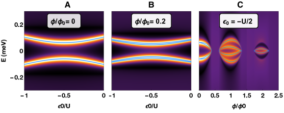
Figure S3: Suppressed Zeeman splitting in the zeroth lobe and ZBAs induced by singlet-doublet parity crossings. (A and B) Poles of Eq. (S11) shown in blue superimposed to the numerical DOS as a function of the bias voltage $V$ and $\epsilon_{0}/U$ for two different normalized fluxes $\phi/\phi_{0}$ within the zeroth LP lobe, namely 0 and 0.2, respectively. (C) Poles and numerical DOS versus $V$ and $\phi/\phi_{0}$ at $\epsilon_{0}=-U/2$. $U=1$ meV, $\Gamma_{S}=0.43$ meV, and $\Gamma_{N}=0.2$ meV. The rest of parameters are the same as in Fig. 4F left panel (see Table S1). Within the zeroth lobe, the LP modulation of the gap together with a small Zeeman energy (even for a sizeable $g=13$) lead to a Zeeman splitting that cannot be experimentally resolved, as shown in (B). Using the above parameters $V_{Z}/\Gamma_{N}=0.45$.

Parity crossings versus flux $\phi$

As it is clear from the previous discussion, the fate of the GS character with external flux depends on the initial $\phi=0$ position of the system parameters in the $\epsilon_{0}/U$-$\Gamma_{S}/U$ plane. If these parameters are far away from the singlet-doublet boundary, the system will remain in the same GS for moderate fluxes. This is the case of Figs. 4, A, B and D, of the main text where the system remains in a singlet GS for fluxes deep into the first lobe. Since the GS is a singlet, a further effect, apart from LP modulation, is the Zeeman splitting of the subgap excitations. However, such Zeeman splitting is not clearly seen in the experiment across the zeroth lobe. Figure S3 shows theoretical calculations in this regime. In agreement with the experiment, the Zeeman splitting in the zeroth lobe cannot be resolved. This can be explained by the combined effect of the LP gap closing (which strongly modifies the linear Zeeman dispersion at low $B$ fields), the small Zeeman energy (even for a sizeable $g=13$) and the tunneling broadening of the lines (compare poles with the full DOS). In Fig. S3B $V_{Z}/\Gamma_{N}=0.45$.

When the initial point is relatively close to the dome boundary, one or more singlet-doublet transitions will probably occur at moderate fluxes. In particular, Fig. 5I in the main text discusses how we approach the singlet-doublet transition that we present in Figs. 5, A, B and C, (the corresponding point in parameter space for said figure is marked by a yellow circle). The system starts in a singlet GS for $\phi=0$. As the applied flux increases, the dome approaches the yellow point which crosses the singlet-doublet line at $\phi\approx\phi_{0}$, remaining in the doublet phase afterwards. We note that, if we had a system with an initial singlet state slightly different from the one of the yellow point, but same $g$-factor, it may cross the dome at very different values of $\phi$. For example, experimental points in this phase diagram with the same $\Gamma_{S}$ but slightly different gate voltage outside the region $\epsilon_{0}/U\in[-1,0]$ (red circle), or for the same gate voltage ($\epsilon_{0}$) but larger coupling to the SC $\Gamma_{S}$ (light blue circle), are still in the singlet phase for the largest $\phi$ shown here. This exemplifies how QD physics can lead to $\phi$-induced parity crossings, and concomitant zero bias anomalies in transport, at very different points in the parameter space of this complex interplay of different physical phenomena.

The simulation for the specific parity crossing of Fig. 5B is shown in Fig. 5, G and H, where we plot the poles of Eq. (S11), shown in black, superimposed to the numerical DOS as a function of bias voltage $V$ and magnetic flux.

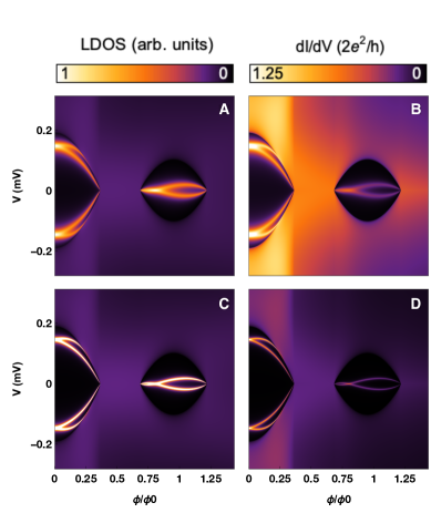
Figure S4: Comparison between the numerical LDOS (A and C) and the simulated $dI/dV$ (B and D) in the tunneling limit, as a function of magnetic flux $\phi/\phi_{0}$ in a QD-SC full shell NW. We assume a constant coupling $\Gamma_{N}$ to the normal probe and compare the two quantities for two small values of $\Gamma_{N}/\Gamma_{S}$ (0.16 and 0.04 in the top and bottom rows, respectively). In general, while the relative magnitude of the two quantities may differ quantitatively, the evolution of subgap ABSs are accurately captured by the peaks of the tunneling $dI/dV$ (the parameters can be found in Table S1).

Differential conductance versus local density of states

A common technique to experimentally measure the spectral density of a mesoscopic system is to use a metallic probe weakly coupled to the system. Under a number of ideal assumptions (weak, energy-independent coupling $\Gamma_{N}$, featureless density of states in the probe with a sufficient energy range, and sufficiently low temperatures), the tunneling differential conductance $g(V)=dI/dV$ at a bias $V$ from the probe into a certain point in the system is proportional to the system’s local density of states (LDOS) at energy $\epsilon=eV$. This is the basis of transport spectroscopy.

In realistic conditions, however, particularly in the case of hybrid semiconducting NWs of interest here, one can expect some deviations between the tunneling spectroscopy $g(V)$ and the Bogoliubov-de Gennes (BdG) LDOS($\epsilon$) of the coupled probe-system. In the tunneling limit, sharp peaks in the LDOS (from subgap ABSs) yield peaks in the $dI/dV$ at essentially the same energy. The LDOS peaks are delta functions of weight one, broadened phenomenologically by the N-QD coupling $\Gamma_{N}$. In contrast, the corresponding subgap $dI/dV$ is given by Andreev reflection peaks of height $\leq 2e^{2}/h$ (or $\leq 4e^{2}/h$ for spin-degenerate states), depending on the relative transparencies of N-QD and QD-S barriers. The width of the $dI/dV$ peaks also depends on the specific microscopic details of these barriers and may exhibit some bias dependence. Other typical deviations include bias asymmetries $g(-V)\neq g(V)$  (?), which are absent in the BdG LDOS by construction and, more generally, differences in the relative magnitude between subgap and above-gap values when comparing $dI/dV$ and LDOS. If we consider more realistic coupling models for the probe, across, say, an extended smooth barrier, the relative $dI/dV$ visibility of different spectral LDOS features, particularly above the gap, might change. An example of this effect relevant to Majorana wires with QDs was discussed in Ref.  (?), where a smooth extended barrier between probe and system washed out small-momenta spectral features in the $dI/dV$, such as the topological gap inversion. In spite of these subtleties, tunneling spectroscopy remains a valuable technique to access the spectral density of a hybrid NW such as ours, and in particular to measure the evolution of the energy of subgap Andreev bound states, as long as $\Gamma_{N}$ is smaller than other relevant energy scales in the system ($\Gamma_{S},k_{B}T,\Delta$ and $U$).

To get a more precise sense of how the $dI/dV$ approximates the LDOS in our QD-SC system, we have computed the two quantities using the same model of Section Model. No further complexity is added to the probe-system coupling beyond a constant spin-independent $\Gamma_{N}$. The subgap $dI/dV$ (Andreev conductance) is then given by $g(V)=g_{0}4\Gamma_{N}^{2}\sum_{\sigma}|G_{12,\sigma}(\omega=eV)|^{2}$, where $g_{0}=2e^{2}/h$ and $G_{12,\sigma}$ is the off-diagonal component of Eq. (S11). An expression for the full $dI/dV$ including above-gap quasiparticle contributions can be found in Refs.  (?, ?). In Fig. S4 we show the full $dI/dV$ and the LDOS for two values of $\Gamma_{N}/\Gamma_{S}\ll 1$ (tunneling limit). In general, the $dI/dV$ peak heights are bias dependent, and their height relative to the quasiparticle conductances above the gap depends on $\Gamma_{N}$. Far from the tunneling limit, i.e. $\Gamma_{N}/\Gamma_{S}\gtrsim 1$, the $dI/dV$ peaks might even acquire energy shifts for increasing $\Gamma_{N}$ (not shown). In the tunneling regime of interest here, the subgap $dI/dV$ always tracks the evolution of ABSs in the LDOS as a function of parameters in a very accurate way. Thus, the only effect of a finite $\Gamma_{N}\ll\Gamma_{S}$ is merely to induce a finite broadening in the subgap peaks, both in the LDOS and the $dI/dV$ (compare the upper row with the lower row in Fig. S4).

Since the fine details of the probe-QD and QD-SC couplings are largely unknown in our devices, we opt in the main text to directly simulate the intrinsic LDOS of the simplified QD-SC model explained above, and compare it to the measured tunneling $dI/dV$ spectroscopy. Given the good match of our theory simulations of ABS levels to the measured evolution of $dI/dV$ peaks, we conclude that microscopic barrier details are inessential to the interpretation of our experiment.

Additional experimental data

Materials and methods

The hexagonal InAs NWs, with a diameter of about $110\,$\mathrm{n}\mathrm{m}$$, were grown via the VLS technique and the $30\,$\mathrm{n}\mathrm{m}$$ Al shell was epitaxially grown in situ, giving a highly transparent semiconductor-SC interface  (?, ?). The NWs were deposited on a heavily doped silicon substrate covered with $285\,$\mathrm{n}\mathrm{m}$$ of silicon oxide. The Al shell is completely removed from one side of the NW via transene etching and the bare InAs is employed as a tunnel barrier. The Al shell, $L$, is longer than $1.5\,$\mathrm{\SIUnitSymbolMicro}\mathrm{m}$$ for all the measured devices. Hence, effects of overlapping potential MZMs could be neglected as $L$ is much larger than the coherence length  (?, ?). The gates and contacts consist of normal-metal ($5\,$\mathrm{n}\mathrm{m}$$/$180\,$\mathrm{n}\mathrm{m}$$ Ti/Au bilayer). The differential conductance, $dI/dV$, was measured via a lock-in technique in a dilution refrigerator with a base temperature of $20\,$\mathrm{m}\mathrm{K}$$. Tunneling $dI/dV$ measurements of the superconducting gap as a function of flux are used in Fig. S5 and Table S2 to extract estimates for relevant NW parameters (NW radius $R$, shell thickness $d$ and coherence length $\xi$) in different devices. This is done by fitting the shape of the LP lobes against the Ginzburg-Landau theory predictions, see Eqs. (S5) and (S6). Note that slightly different values of the parameters produce fittings with similar level of accuracy, see white and green dotted curves in Fig. S5 for device A. This means that the values of these parameters can be estimated only approximately.

Kondo effect and g-factor

As mentioned, YSR singlets are the superconducting counterparts of Kondo singlets and a full screening of the quantum impurity spin is expected when the exchange between the QD and the SC is large enough, such that $k_{B}T_{K}\approx\Delta$. While previous works have studied this doublet-YSR singlet quantum phase transition (QPT) by a controlled tuning of $\Gamma_{S}$  (?), we here can reach a Kondo regime owing to the destructive LP regions where the gap is suppressed. From Eq. (1) in the main text, we can extract an effective exchange coupling $J=2\Gamma_{S}/U$ (at zero magnetic field), which enters the expression of the Kondo temperature $k_{B}T_{K}\approx 0.3\sqrt{U\Gamma_{S}}e^{-\frac{\pi U}{8\Gamma_{S}}}\approx 0.2U\sqrt{J}e^{-\frac{\pi}{4J}}$ at the symmetry point (the dashed line in Fig. 3A of the main text). Using the experimental values for $U$ and $\Gamma_{S}$, we get $k_{B}T_{K}\approx 0.044\;\rm{meV}\approx 0.24\Delta(\phi=0)$. Owing to the LP reduction of the gap, a full Kondo effect is expected to develop when $k_{B}T_{K}\approx\Delta(\phi)$  (?), which first happens at $\phi\approx 0.35\phi_{0}$. Indeed, we find a symmetric pair of excitations that appear in the first destructive LP regime, starting at $\approx 50$mT which corresponds to $0.33\phi_{0}$ (cyan trace in Fig. S9C), that we interpret as cotunneling processes through a spin-split Kondo resonance, supporting the previous picture. At larger fluxes, the gap reopens, and the system goes back to a doublet GS with YSR singlet subgap excitations. This remarkable modulation from YSR singlets to Kondo and back is only possible due to the destructive LP effect. This YSR-Kondo QPT mediated by the LP effect occurs for typical QD parameters around the same flux regions where Majoranas are predicted to occur in full-shell NWs  (?, ?), which adds further complexity to the problem. This Kondo interpretation is supported by the decreasing height of the conductance peaks for increasing temperatures (Fig. S9E). As expected, the hard superconducting gap precludes the formation of a Kondo resonance, which is absent in the zeroth and first lobe. On the contrary, the soft gap in the second lobe allows the formation of an above-gap split Kondo resonance, which, in this regime, coexists with the YSR states  (?, ?) (see line traces in Fig. S9C). The progression of the Kondo peaks in magnetic field allows for an estimation of the NW’s $g$-factor. The extracted values are $g=6.4\pm 0.8$ in the first destructive region, $g=9.2\pm 0.3$ in the second destructive one and $g=10.5\pm 0.1$ from the end of the second lobe to $B=900\,$\mathrm{m}\mathrm{T}$$ (Fig. S10). The data indicate a non linear behaviour of $g$ with the magnetic field. This apparent non-linearity relates to the LP effect as the flux which can penetrate the core of the NW depends on the magnetic field value. Nonlinearities of the effective $g$-factor owing to Kondo interactions in a superconducting system are also expected  (?).

Name of the device	$R$ [nm]	$d$ [nm]	$\xi$ [nm]
A	64	24	160
A2	60	28	150
F	60	28	165
G	61	29	150
H	67	23	160
I	66	21	165
J	60	28	175
K	66	21	165
L	60	27	160
M	60	29	175

Table S2: Dimensions of short junction devices. NW parameters extracted from the analysis of Fig. S5. Going from flux $\phi$ to magnetic field $B$ we assumed a circular effective section of radius $R+10\rm{nm}$ which captures the finite penetration length of $B$ in the SC shell and is required to achieve experimental agreement.

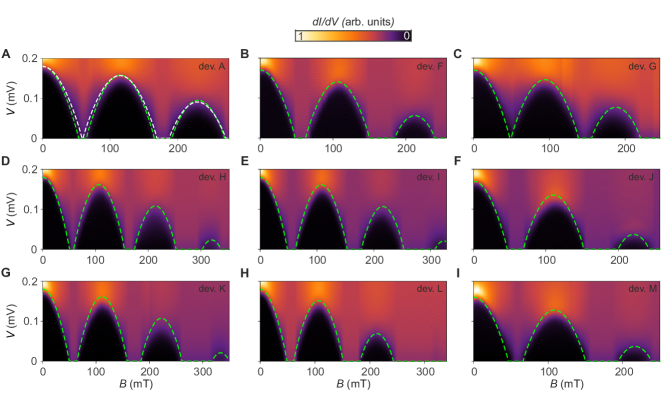
Figure S5: Little-Parks measurement used for extracting the NW parameters for all short-junction devices. $dI/dV$ as a function of $V$ and $B$ for device A and F-M. The superimposed LP theory curves allow us to extract the NW parameters from the lobes using Eqs. (S5) and (S6). For device A the white dashed curve represents the case where $R=60\,$\mathrm{n}\mathrm{m}$$, $d=28\,$\mathrm{n}\mathrm{m}$$ and $\xi=150\,$\mathrm{n}\mathrm{m}$$ while the green dashed curve corresponds to $R=64\,$\mathrm{n}\mathrm{m}$$, $d=24\,$\mathrm{n}\mathrm{m}$$ and $\xi=160\,$\mathrm{n}\mathrm{m}$$. For all devices the parameters are summarized in table S2. The linear colorscale is renormalized by the maximum for each panel.

Figure S6: Devices with a short junction. In the right-upper corner of each plot, the letter indicates the device. (A), (C), (E), (G), (I) , (K), (M) and (O) $dI/dV$ as a function of $V$ and $V_{\textrm{bg}}$ for devices with a short junction in absence of magnetic fields. No ABSs are present for these devices because of the short junction. More concretely, device F has $X\approx 95\,$\mathrm{n}\mathrm{m}$$, device G has $X\approx 60\,$\mathrm{n}\mathrm{m}$$, device H has $X\approx 85\,$\mathrm{n}\mathrm{m}$$, device I has $X\approx 70\,$\mathrm{n}\mathrm{m}$$, device J has $X\approx 90\,$\mathrm{n}\mathrm{m}$$, device K has $X\approx 60\,$\mathrm{n}\mathrm{m}$$, device L has $X\approx 80\,$\mathrm{n}\mathrm{m}$$ and device M has $X\approx 40\,$\mathrm{n}\mathrm{m}$$. (B), (D), (F), (H), (J), (L), (N) and (P) $dI/dV$ as a function of $V$ and $B$ at a fixed value of $V_{\textrm{bg}}$. The magnetic field scans have been taken at $V_{\textrm{bg}}=-12\,$\mathrm{V}$$ for device F, at $V_{\textrm{bg}}=-32\,$\mathrm{V}$$ for device G, at $V_{\textrm{bg}}=-12\,$\mathrm{V}$$ for device H, at $V_{\textrm{bg}}=-7.5\,$\mathrm{V}$$ for device I, at $V_{\textrm{bg}}=-19\,$\mathrm{V}$$ for device J, at $V_{\textrm{bg}}=-15.5\,$\mathrm{V}$$ for device K, at $V_{\textrm{bg}}=-5\,$\mathrm{V}$$ for device L and at $V_{\textrm{bg}}=-30\,$\mathrm{V}$$ for device M. The different shapes and positions of the lobes are due to the slightly different NW and Al shell dimensions. However, neither ZBPs nor other subgap features are observed.

Figure S7: Line traces of short junction devices at the center of the zeroth and first lobe. (A) Line-cuts taken from Fig. S6B. (B) Line-cuts taken from Fig. S6D. (C) Line-cuts taken from Fig. S6F. (D) Line-cuts taken from Fig. S6H. (E) Line-cuts taken from Fig. S6J. (F) Line-cuts taken from Fig. S6L. (G) Line-cuts taken from Fig. S6N. (H) Line-cuts taken from Fig. S6P.

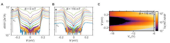
Figure S8: Subgap conductance evolution for device A as a function of the backgate voltage. (A) Line-cuts extracted from the measurement shown in Fig. 1C, ranging from $V_{\textrm{bg}}=-20.4\,$\mathrm{V}$$ (lower trace) to $V_{\textrm{bg}}=-6\,$\mathrm{V}$$ (upper trace), equally spaced. (B) Line-cuts taken at $B=116$ mT, i.e. in the middle of the first lobe. The line-cuts range from $V_{\textrm{bg}}=-19.6\,$\mathrm{V}$$ (lower trace) to $V_{\textrm{bg}}=-6.4\,$\mathrm{V}$$ (upper trace), equally spaced. No signature of MZMs is observed independently of the junction transparency. (C) $dI/dV$ as a function of $V$ and $V_{\textrm{bg}}$ for device A, at $B=116\,$\mathrm{m}\mathrm{T}$$, namely in the middle of the first lobe. The line-cuts of (B) are taken from (C).

Figure S9: Kondo effect in the Little-Parks regime with a doublet GS from device B. (A) Same plot as Fig. 3D but without the analytical solution superimposed. (B) and (C) Line traces extracted from (A) for different values of $B$. The line traces in (B) show that ABSs in the doublet GS, indicated with 1, increase their energy with magnetic field. In the absence of magnetic field, $\zeta\approx\pm 63\,$\mathrm{\SIUnitSymbolMicro}\mathrm{V}$$ (deep blue trace), while at $B=110\,$\mathrm{m}\mathrm{T}$$ (green trace) $\zeta\approx\pm 80\,$\mathrm{\SIUnitSymbolMicro}\mathrm{V}$$, even though the superconducting gap is smaller at finite $B$. (C) Line traces showing the presence of a split Kondo peak (K) in the destructive regimes, namely at $B=60\,$\mathrm{m}\mathrm{T}$$ (cyan trace), at $B=170\,$\mathrm{m}\mathrm{T}$$ (purple trace) and at $B=280\,$\mathrm{m}\mathrm{T}$$ (red trace). Furthermore, the Kondo peaks coexist with superconductivity and ABSs in the 2L (orange trace taken at $B=230\,$\mathrm{m}\mathrm{T}$$). (D) Numerical simulation of the $dI/dV$ versus bias voltage $V$ and magnetic flux $\phi/\phi_{0}$ in a QD-S (modelled as a superconducting Anderson model in the Hartree-Fock approximation), with the SC in the destructive LP regime and the QD in a doublet GS (parameters can be found in Table S1). (E) $dI/dV$ as a function of $V$ at $B=60\,$\mathrm{m}\mathrm{T}$$ for different temperatures. The split Kondo peaks broaden and decrease their conductance forming a ZBP at $T=240\,$\mathrm{m}\mathrm{K}$$, while they completely disappear for $T=2817\,$\mathrm{m}\mathrm{K}$$. (F) Current, $I$, as a function of $V$ and $V_{\textrm{bg}}$ for an out-of-plane magnetic field of $50\,$\mathrm{m}\mathrm{T}$$ that destroys superconductivity revealing Coulomb diamonds. The charging energy is $\approx 2.5\,$\mathrm{m}\mathrm{e}\mathrm{V}$$.

Figure S10: Kondo data for higher magnetic fields, from device B. (A) $dI/dV$ as a function of $V$ and $B$ for $V_{\textrm{bg}}=-2.62\,$\mathrm{V}$$, hence in the doublet GS. (B) Line traces extracted from (A) for $B=550\,$\mathrm{m}\mathrm{T}$$ (blue trace) and for $B=800\,$\mathrm{m}\mathrm{T}$$ (green trace).

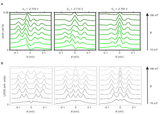
Figure S12: ZBP in the first lobe due to ABSs in device B. (A) Line traces extracted from the first lobe of Fig. 4E (left, center and right panels) of the main text, showing $dI/dV$ as a function of $V$ from $B=74\,$\mathrm{m}\mathrm{T}$$ (lower one) to $B=158\,$\mathrm{m}\mathrm{T}$$ (upper one); they are shifted by $0.01\frac{e^{2}}{h}$ with respect to each other. (B) Numerical simulations of (A) extracted from Fig. 4F (left, center and right panels) of the main text.

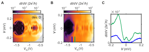
Figure S13: Dependence of ZBP on the backgate voltage and additional data for device D. (A) $dI/dV$ as a function of $V$ and $V_{\textrm{bg}}$ at in absence of magnetic field. Multiple ABSs are clearly visible. The dashed pink line indicates where the magnetic field scan shown in Fig. 5B was taken. (B) $dI/dV$ as a function of $V$ and $V_{\textrm{bg}}$ at $B=108\,$\mathrm{m}\mathrm{T}$$, i.e., in the first lobe. The presence of a ZBP depends on $V_{\textrm{bg}}$, proving that it has no topological origin. (C) Line traces extracted from (B); the blue curve corresponds to $V_{\textrm{bg}}=-1.25\,$\mathrm{V}$$ while the green one to $V_{\textrm{bg}}=-1.34\,$\mathrm{V}$$.

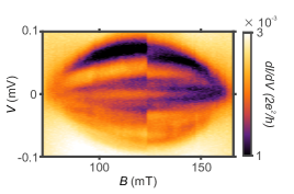
Figure S14: Zoom of Fig. 5C. $dI/dV$ as a function of $B$ and $V$; same as Fig. 5C but with a finer resolution.

References

- 1. J. A. Sauls, Philos. Trans. Royal Soc. A 376 (2018).
- 2. J. Pillet, et al., Nat. Phys. 6, 965 (2010).
- 3. A. Eichler, et al., Phys. Rev. Lett. 99 (2007).
- 4. L. Bretheau, C. O. Girit, H. Pothier, D. Esteve, C. Urbina, Nature 499, 312 (2013).
- 5. T. Dirks, et al., Nat. Phys. 7, 386 (2011).
- 6. E. J. H. Lee, et al., Phys. Rev. Lett. 109, 186802 (2012).
- 7. W. Chang, V. E. Manucharyan, T. S. Jespersen, J. Nygård, C. M. Marcus, Phys. Rev. Lett. 110, 217005 (2013).
- 8. E. J. H. Lee, et al., Nat. Nanotechnol. 9, 79 (2014).
- 9. A. Jellinggaard, K. Grove-Rasmussen, M. H. Madsen, J. Nygård, Phys. Rev. B 94, 064520 (2016).
- 10. E. J. H. Lee, et al., Phys. Rev. B 95, 180502 (2017).
- 11. K. Grove-Rasmussen, et al., Nat. Commun. 9, 2376 (2018).
- 12. Z. Su, et al., Phys. Rev. Lett. 121, 127705 (2018).
- 13. C. Jünger, et al., Communications Physics 2, 1 (2019).
- 14. C. Jünger, et al., Phys. Rev. Lett. 125, 017701 (2020).
- 15. Z. Su, et al., Phys. Rev. B 101, 235315 (2020).
- 16. C. Janvier, et al., Science 349, 1199 (2015).
- 17. M. Hays, et al., Nature Physics (2020).
- 18. R. M. Lutchyn, J. D. Sau, S. Das Sarma, Phys. Rev. Lett. 105, 077001 (2010).
- 19. Y. Oreg, G. Refael, F. von Oppen, Phys. Rev. Lett. 105, 177002 (2010).
- 20. R. Aguado, Riv. Nuovo Cimento 40, 523 (2017).
- 21. R. M. Lutchyn, et al., Nat. Rev. Mater. 3, 52 (2018).
- 22. E. Prada, et al., Nat. Rev. Phys. 2, 575 (2020).
- 23. V. Mourik, et al., Science 336, 1003 (2012).
- 24. S. M. Albrecht, et al., Nature 531, 206 (2016).
- 25. M. T. Deng, et al., Science 354, 1557 (2016).
- 26. F. Nichele, et al., Phys. Rev. Lett. 119, 136803 (2017).
- 27. H. Zhang, et al., Nat. Commun. 8, 16025 EP (2017).
- 28. Ö. Gül, et al., Nat. Nanotechnol. 13, 192 (2018).
- 29. E. Prada, P. San-Jose, R. Aguado, Phys. Rev. B 86, 180503 (2012).
- 30. G. Kells, D. Meidan, P. W. Brouwer, Phys. Rev. B 86, 100503 (2012).
- 31. C.-X. Liu, J. D. Sau, T. D. Stanescu, S. D. Sarma, Phys. Rev. B 96, 075161 (2017).
- 32. C. Moore, T. D. Stanescu, S. Tewari, Phys. Rev. B 97, 165302 (2018).
- 33. C. Reeg, O. Dmytruk, D. Chevallier, D. Loss, J. Klinovaja, Phys. Rev. B 98, 245407 (2018).
- 34. J. Chen, et al., Phys. Rev. Lett. 123, 107703 (2019).
- 35. A. Vuik, B. Nijholt, A. R. Akhmerov, M. Wimmer, SciPost Phys. 7, 61 (2019).
- 36. J. Avila, F. Peñaranda, E. Prada, P. San-Jose, R. Aguado, Communications Physics 2, 133 (2019).
- 37. H. Pan, S. D. Sarma, Phys. Rev. Research 2, 013377 (2020).
- 38. J. Cayao, E. Prada, P. San-Jose, R. Aguado, Phys. Rev. B 91, 024514 (2015).
- 39. W. Chang, et al., Nat. Nanotechnol. 10, 232 (2015).
- 40. S. Vaitiekėnas, et al., Science 367, eaav3392 (2020).
- 41. F. Peñaranda, R. Aguado, P. San-Jose, E. Prada, Phys. Rev. Research 2, 023171 (2020).
- 42. S. Vaitiekėnas, P. Krogstrup, C. M. Marcus, Phys. Rev. B 101, 060507 (2020).
- 43. D. Sabonis, et al., Phys. Rev. Lett. 125, 156804 (2020).
- 44. G. Schwiete, Y. Oreg, Phys. Rev. B 82, 214514 (2010).
- 45. N. Shah, A. Lopatin, Phys. Rev. B 76, 094511 (2007).
- 46. See supplementary materials.
- 47. W. A. Little, R. D. Parks, Phys. Rev. Lett. 9, 9 (1962).
- 48. Y. Liu, et al., Science 294, 2332 (2001).
- 49. C. Reeg, D. Loss, J. Klinovaja, Phys. Rev. B 97, 165425 (2018).
- 50. A. E. G. Mikkelsen, P. Kotetes, P. Krogstrup, K. Flensberg, Phys. Rev. X 8, 031040 (2018).
- 51. B. D. Woods, S. Das Sarma, T. D. Stanescu, Phys. Rev. B 99, 161118 (2019).
- 52. A. A. Kopasov, A. S. Mel’nikov, Phys. Rev. B 101, 054515 (2020).
- 53. E. Vecino, A. Martín-Rodero, A. L. Yeyati, Phys. Rev. B 68, 035105 (2003).
- 54. T. Meng, S. Florens, P. Simon, Phys. Rev. B 79, 224521 (2009).
- 55. R. S. Deacon, et al., Phys. Rev. Lett. 104, 076805 (2010).
- 56. R. Žitko, J. S. Lim, R. López, R. Aguado, Phys. Rev. B 91, 045441 (2015).
- 57. L. Yu, Acta. Phys. Sin. 21, 75 (1965).
- 58. H. Shiba, Prog. Theor. Phys. 40, 435 (1968).
- 59. A. Rusinov, Sov. Phys. JETP 9, 85 (1969).
- 60. A. V. Balatsky, I. Vekhter, J.-X. Zhu, Rev. Mod. Phys. 78, 373 (2006).
- 61. V. Koerting, B. M. Andersen, K. Flensberg, J. Paaske, Phys. Rev. B 82, 245108 (2010).
- 62. G. Kiršanskas, M. Goldstein, K. Flensberg, L. I. Glazman, J. Paaske, Phys. Rev. B 92, 235422 (2015).
- 63. A. Melo, C.-X. Liu, P. Rożek, T. Ö. Rosdahl, M. Wimmer, SciPost Phys. 10, 37 (2021).
- 64. Experimental data for: Non-topological zero bias peaks in full-shell nanowires induced by flux tunable Andreev states (2021); https://doi.org/10.15479/AT:ISTA:9389.
- 65. Simulation code for: Non-topological zero bias peaks in full-shell nanowires induced by flux tunable Andreev states (2021); https://doi.org/10.5281/zenodo.4768060.
- 66. L. Pavešić, D. Bauernfeind, R. Žitko, arXiv:2101.10168 (2021).
- 67. J. C. E. Saldaña, et al., arXiv:2101.10794 (2021).
- 68. A. Larkin, A. Varlamov, Theory of Fluctuations in Superconductors (Oxford University Press, 2005).
- 69. R. P. Groff, R. D. Parks, Phys. Rev. 176, 567 (1968).
- 70. J. Bardeen, Rev. Mod. Phys. 34, 667 (1962).
- 71. A. Abrikosov, Soviet Physics JETP 12, 337 (1961).
- 72. P. G. de Gennes, Superconductivity in Metals and Alloys (W. A. Benjamin, Inc., New York, 1966).
- 73. S. Skalski, O. Betbeder-Matibet, P. R. Weiss, Phys. Rev. 136, A1500 (1964).
- 74. A. Martín-Rodero, A. L. Yeyati, Journal of Physics: Condensed Matter 24, 385303 (2012).
- 75. J. Bauer, A. Oguri, A. C. Hewson, Journal of Physics: Condensed Matter 19, 486211 (2007).
- 76. M. Žonda, V. Pokorný, V. Janiš, T. Novotný, Scientific Reports 5, 8821 (2015).
- 77. N. Wentzell, S. Florens, T. Meng, V. Meden, S. Andergassen, Phys. Rev. B 94, 085151 (2016).
- 78. M. Žonda, V. Pokorný, V. Janiš, T. Novotný, Phys. Rev. B 93, 024523 (2016).
- 79. A. García Corral, et al., Phys. Rev. Research 2, 012065 (2020).
- 80. T. Yoshioka, Y. Ohashi, J. Phys. Soc. Jpn 69, 1812 (2000).
- 81. J. Barański, T. Domański, J. Phys. Condens. Matter 25, 435305 (2013).
- 82. P. Krogstrup, et al., Nat. Mater. 14, 400 (2015).
- 83. S. D. Sarma, J. D. Sau, T. D. Stanescu, Phys. Rev. B 86, 220506 (2012).