Optimal Data Detection and Signal Estimation
in Systems with Input Noise

Abstract

Practical systems often suffer from hardware impairments that already appear during signal generation. Despite the limiting effect of such input-noise impairments on signal processing systems, they are routinely ignored in the literature. In this paper, we propose an algorithm for data detection and signal estimation, referred to as Approximate Message Passing with Input noise (AMPI), which takes into account input-noise impairments. To demonstrate the efficacy of AMPI, we investigate two applications: Data detection in large multiple-input multiple-output (MIMO) wireless systems and sparse signal recovery in compressive sensing. For both applications, we provide precise conditions in the large-system limit for which AMPI achieves optimal performance. We furthermore use simulations to demonstrate that AMPI achieves near-optimal performance at low complexity in realistic, finite-dimensional systems.

I Introduction

We consider a general class of data detection and signal estimation problems in a noisy linear channel affected by input noise. As illustrated in fig:sysmodel, we are interested in recovering the $N$-dimensional input signal $\mathbf{s}\in\mathbb{C}^{N}$ observed from the following model. The input signal $\mathbf{s}$ with prior distribution $p(\mathbf{s})=\prod_{\ell=1}^{N}p(s_{\ell})$ is affected by input-noise characterized by the statistical relation $p(\mathbf{x}|\mathbf{s})=\prod_{\ell=1}^{N}p(x_{\ell}|s_{\ell})$. The generality of this input-noise model captures a wide range of hardware and system impairments, including hardware non-idealities that exhibit statistical dependence between impairments and the input signal (e.g., phase noise) as well as deterministic effects (e.g., non-linearities). The impaired signal $\mathbf{x}\in\mathbb{C}^{N}$, which we refer to as the effective input signal, is then passed to a noisy linear transform that is modeled as

$$\mathbf{y}=\mathbf{H}\mathbf{x}+\mathbf{n}.$$ (1)

Here, the vector $\mathbf{y}\in\mathbb{C}^{M}$ is the measured signal and $M$ denotes the number of measurements, the system matrix $\mathbf{H}\in\mathbb{C}^{M\times N}$ represents the measurement process, and the vector $\mathbf{n}\in\mathbb{C}^{M}$ models measurement noise. We assume that the entries of the noise vector $\mathbf{n}$ are i.i.d. circularly-symmetric complex Gaussian with variance $N_{0}$. In what follows, we make use of the system ratio defined as $\beta={N}/{M}$ and the following definitions:

Definition 1.

We define the large system limit by fixing the system ratio $\beta=N/M$ and by letting $N\to\infty$.

Definition 2.

A matrix $\mathbf{H}$ describes uniform linear measurements if the entries of $\mathbf{H}$ are i.i.d. circularly-symmetric complex Gaussian with variance $1/M$, i.e., $H_{i,j}\sim\mathcal{C}\mathcal{N}(0,1/M)$.

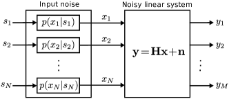
Figure 1: Illustration of a noisy linear system affected by input noise. The input signal $\mathbf{s}$ is corrupted by input noise, resulting in the effective input signal $\mathbf{x}$ that is observed through a noisy linear system. The goal is to recover the input signal $\mathbf{s}$ from the noisy observations $\mathbf{y}$.

I-A Two Application Examples

While numerous real-world systems suffer from input noise, we focus on two prominent scenarios.

I-A1 Massive MIMO Data Detection

Massive multiple-input multiple-output (MIMO) is one of the core technologies in fifth-generation (5G) wireless systems [2]. The idea is to equip the infrastructure base-stations with hundreds of antenna elements while simultaneously serving a smaller number of users. One critical challenge in the realization of this technology is the computational complexity of data detection at the base-station [3]. While recent results have shown that the large dimensionality of massive MIMO can be exploited to design near-optimal data-detection algorithms [4, 5, 6] using approximate message passing (AMP) [7], these methods ignore the fact that realistic communication systems are affected by impairments that already arise at the transmitter [8, 9]. In this paper, we introduce AMPI (short for AMP with input noise), which mitigates transmit-side RF impairments during data detection. AMPI outperforms existing data-detection methods, e.g., [5], that ignore the presence of input-noise impairments at virtually no additional computational complexity.

fig:MIMO illustrates the symbol error-rate (SER) performance of AMPI in a symmetric massive MIMO system with $128$ user equipments (UEs) transmitting QPSK and $128$ base-station (BS) antennas. As in [8, 10, 9], the input noise is modeled as complex Gaussian noise. We see that AMPI outperforms the LAMA algorithm [4, 5], which achieves—under certain conditions on the MIMO system—the error-rate performance of the individually-optimal (IO) data detector in absence of input noise. AMPI entails virtually no complexity increase over LAMA and achieves comparable SER to whitening-based methods [8], which are optimal for Gaussian input noise but result in prohibitively high complexity in massive MIMO.

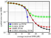
(a) Symbol-error rate (SER) versus average SNR in a $128$ user equipment (UE), $128$ base-station antenna massive MIMO system with QPSK.

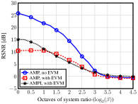
(b) Reconstruction SNR of a sparse signal recovery task for a $5\%$ sparse signal of dimension $N=1000$ and 20 dB SNR.

Figure 2: Simulation results of two applications of the proposed AMPI algorithm in massive MIMO and compressive sensing with $\textit{EVM}=-10$ dB input noise. AMPI yields significant improvements compared to methods that ignore input noise and achieves comparable performance to whitening-based methods that entail prohibitive complexity for the considered system dimensions.

I-A2 Compressive Sensing Signal Recovery

Compressive sensing (CS) enables sampling and recovery of sparse signals at sub-Nyquist rates [11, 12]. While the CS literature extensively focuses on systems with measurement noise, numerous practical applications already contain noise on the sparse signal to be recovered; see [13, 14, 15] and the references therein. We will use AMPI to take input-noise into account directly during sparse signal recovery and show substantial improvements compared to that of existing sparse recovery methods for systems with input noise [15] at no additional expense in complexity.

fig:NF shows the recovery signal-to-noise-ratio (RSNR) of compressive sensing scenario in which we recover a $N=1000$ dimensional sparse signal in the presence of input noise with an error-vector magnitude (EVM) of $-10$ dB. The RSNR is plotted for different system ratios $\beta$. The signal is assumed to have $5\%$ sparsity and an SNR of $20$ dB; the non-zero entries are i.i.d. standard normal. AMPI significantly improves the reconstruction SNR over AMP which ignores input noise.

I-B Contributions

We propose AMPI and provide precise conditions for which it yields optimal performance in data detection and signal estimation applications. Depending on the application, we use the following optimality criteria. For massive MIMO data detection, optimality is achieving the same error-rate performance as the individually-optimal (IO) data detector [5, 16], which solves the following minimization problems:

$$\hat{s}_{\ell}^{\textnormal{IO}}=\operatorname*{arg\;min}_{\tilde{s}_{\ell}\in\mathcal{O}}\,\mathbb{P}\!\left(\tilde{s}_{\ell}\neq s_{\ell}\right)\!,\quad\ell=1,\ldots,N.$$ (2)

Here, $\mathcal{O}$ is a finite set containing possible transmit symbols—in wireless systems this set corresponds to the transmit constellation, e.g., quadrature amplitude modulation (QAM). For signal estimation, optimality is defined by minimizing the mean-squared error (MSE)

$$\hat{\mathbf{s}}^{\textnormal{O}}=\operatorname*{arg\;min}_{\tilde{}\mathbf{s}\in\mathbb{C}^{N}}\,\textstyle\frac{1}{N}\left\|\tilde{}\mathbf{s}-\mathbf{s}\right\|^{2}\!.$$ (3)

Here, the superscript O in $\hat{s}_{\ell}^{\textnormal{O}}$, $\ell=1,\ldots,N$, stands for optimal. To solve eq:IOproblem or eq:MMSEproblem, we need to compute the MAP or minimum MSE (MMSE) estimate of the marginal posterior distribution $p(s_{\ell}|\mathbf{y},\mathbf{H})$ for all $\ell=1,\dots,N$. Computing the marginal distribution for large-dimensional systems is one of the key challenges in data detection and signal estimation problems as its requires prohibitive complexity [17]. We propose AMPI, which achieves optimal performance in the large-system limit and for uniform linear measurements. Our optimality conditions are derived via the state-evolution (SE) framework [18, 19] of approximate message passing (AMP) [20, 21, 22]. For both applications, we demonstrate the efficacy and low-complexity of AMPI in more realistic, finite-dimensional systems.

I-C Related Results

The effect of input-noise (often called transmit-side impairments) on the performance of communication systems has been studied in [10, 8, 9, 23, 10, 24, 25, 26, 27, 28, 29, 30, 31]. Most of these papers use a Gaussian input-noise model, which assumes that the input noise is i.i.d. additive Gaussian noise and independent of the transmit signal $\mathbf{s}$. While the accuracy of this model has been confirmed via real-world measurements [8] for MIMO systems that use orthogonal frequency-division multiplexing (OFDM), it may not be accurate in other scenarios. AMPI is a practical data detection method that allows us to study the fundamental performance of more general input-noise models, which may exhibit statistical dependence with the transmit signal and even include deterministic nonlinearities. For the well-established Gaussian transmit-noise model, we will show in sec:Opt that the SE equations of AMPI coincide to the “coupled fixed point equations” provided in [9], which demonstrates that AMPI is a practical algorithm that achieves the performance predicted by replica-based channel capacity expressions.

In the compressive sensing literature, input noise causes an effect known as “noise folding” [13, 15, 32]. Reference [15] shows that in the large-system limit, the received SNR is increased by a factor of ${N}/{M}$ due to input noise. Reference [13] shows that an oracle-based recovery procedure that knows the signal support exhibits a $3$ dB loss of reconstructed SNR per octave of sub-sampling. More recently, reference [32] has introduced an $\ell_{1}$-norm based algorithm that reduces the effect of input noise. In contrast to these results, AMPI is a practical signal estimation method that enables one to study the fundamental performance limits of sparse signal recovery in the presence of input noise. We also note that reference [33] investigates signal recovery for a similar model as in eq:sysmodel. The key difference is that AMPI computes an estimate of the original input signal $\mathbf{s}$, whereas the generalized AMP (GAMP) algorithm in [33] recovers the effective input signal $\mathbf{x}$.

I-D Notation

Lowercase and uppercase boldface letters represent column vectors and matrices, respectively. For a matrix $\mathbf{H}$, the conjugate transpose is $\mathbf{H}^{\textnormal{H}}$. The entry on the $i$th row and $j$th column of the matrix $\mathbf{H}$ is $H_{i,j}$; the $k$th entry of a vector $\mathbf{x}$ is $x_{k}$. The $M\times M$ identity matrix is denoted by $\mathbf{I}_{M}$ and the $M\times N$ all-zeros matrix by $\mathbf{0}_{M\times N}$. We define $\left\langle\mathbf{x}\right\rangle=\frac{1}{N}\sum_{k=1}^{N}x_{k}$. The quantities $\|\mathbf{x}\|_{1}$ and $\|\mathbf{x}\|_{2}$ represent the $\ell_{1}$ and $\ell_{2}$ norms of the vector $\mathbf{x}$, respectively. Multivariate real-valued and complex-valued Gaussian probability density functions (pdfs) are denoted by $\mathcal{N}(\mathbf{m},\mathbf{K})$ and $\mathcal{C}\mathcal{N}(\mathbf{m},\mathbf{K})$, respectively, where $\mathbf{m}$ is the mean vector and $\mathbf{K}$ the covariance matrix. The operator $\operatorname{\mathbb{E}}_{X}\!\left[\cdot\right]$ denotes expectation with respect to the probability density function (PDF) of the random variable (RV) $X$; $p(x)$ represents the probability distribution of RV $x$. The notation $a\overset{d}{\rightarrow}b$ represents convergence in distribution of $p(a)$ to $p(b)$. The function $\mathsf{1}(\cdot)$ returns $1$ if its argument is true and $0$ otherwise.

I-E Paper Outline

The rest of the paper is organized as follows. sec:AMPI introduces the AMPI algorithm along with its state evolution (SE) framework. sec:Opt analyzes optimality conditions for AMPI. sec:app1MIMO and sec:app2CS investigate AMPI for data detection in massive MIMO systems and for sparse signal recovery, respectively. We conclude in sec:conclusion.

II AMPI: Approximate Message Passing with Input Noise

We now introduce the message passing algorithm used to derive AMPI. We then develop the complex-valued state-evolution (cSE) framework for AMPI, which will be used in sec:Opt to establish optimality conditions.

II-A Sum-Product Message Passing

As discussed in sec:contributions, the most challenging step in data detection and signal estimation is calculating the marginal posterior distribution. While the problem of marginalizing a distribution is in general NP-hard [17], there exist heuristics that have been successful in certain applications—one of the most prominent marginalizing schemes is message passing.

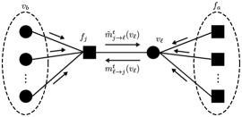
Figure 3: A factor graph illustrating the sum-product message-passing algorithm.

Sum-product message passing is a well-established method to compute the marginal distributions [34, 35]. Consider a joint probability distribution $p(v_{1},\dots,v_{I})$ with random variables taken from the set $\{v_{1},\dots,v_{I}\}$. Suppose that $p(v_{1},\dots,v_{I})$ factors into a product of $J$ functions with subsets of the variable set $\{v_{1},\dots,v_{I}\}$ as their argument: $p(v_{1},\dots,v_{I})=\prod_{j=1}^{J}f_{j}(V_{j})$, where each $V_{j}$ is a subset of the variable set $\{v_{1},\dots,v_{I}\}$ and $\cup_{j=1}^{J}V_{j}=\{v_{1},\dots,v_{n}\}$. Such distributions can be expressed as a factor graphs, which are bipartite graphs consisting of variable nodes to represent each random variable $v_{\ell}$, factor nodes for each factor $f_{j}$, and edges connecting them if the factor node is an argument of the variable node. fig:generalFG illustrates a factor graph with variable nodes (circles) and factor nodes (squares).

For the sum-product message passing algorithm, we consider messages $m_{\ell\rightarrow j}^{t}\!\left(v_{i}\right)$ (from every variable node $v_{i}$ to every factor node $f_{j}$) and $\hat{m}_{j\rightarrow i}^{t}\!\left(v_{i}\right)$ (from every factor node $f_{j}$ to every variable node $v_{i}$) at iteration $t=1,\ldots,{t_{\textnormal{max}}}$ with the equations

$$m_{i\rightarrow j}^{t}\!\left(v_{i}\right) =\prod_{a\neq j}\hat{m}_{a\rightarrow i}^{t-1}\!\left(v_{i}\right)\,$$ (4)

$$\hat{m}_{j\rightarrow i}^{t}\!\left(v_{i}\right) =\int_{\mathbb{C}}f_{j}\!\left(\partial f_{j}\right)\prod_{b\neq i}m_{b\rightarrow j}^{t}\!\left(v_{b}\right)\text{d}(\partial f_{j}\neq v_{i}).$$ (5)

Here, ${t_{\textnormal{max}}}$ is the maximum number of iterations and $\partial f_{j}$ is the set of neighbors of node $f_{j}$ in the graph. After iteratively passing messages between variable nodes and factor nodes, the marginal function of the random variable $v_{i}$ is approximated by the product of all messages directed toward that variable node. If a factor graph is cycle-free, then message-passing converges to the exact marginals. If the factor graph has cycles, then general convergence conditions are unknown [36].

II-B AMPI Derivation

Consider the system model in sec:intro. We are interested in recovering the input signal $\mathbf{s}$ by computing the MAP or MMSE estimate of the marginal posterior distributions $p(s_{\ell}|\mathbf{y},\mathbf{H})$. The marginal distribution $p(s_{\ell}|\mathbf{y},\mathbf{H})$ can be derived from the joint probability distribution $p(\mathbf{s},\mathbf{x},\mathbf{y}|\mathbf{H})$ as follows:

$$p(s_{\ell}|\mathbf{y,H})=\int_{\mathbb{C}^{N-1}}p(\mathbf{s}|\mathbf{y},\mathbf{H})\,\,\text{d}(s_{1},\dots,s_{N}\neq s_{\ell})$$ (6)

$$\quad\propto\int_{\mathbb{C}^{N-1}}\left(\int_{\mathbb{C}^{N}}p(\mathbf{s},\mathbf{x},\mathbf{y}|\mathbf{H})\textnormal{d}\mathbf{x}\right)\text{d}(s_{1},\dots,s_{N}\neq s_{\ell}).$$ (7)

Here, the notation $\text{d}(s_{1},\dots,s_{N}\neq s_{\ell})$ indicates integration over all entries $s_{1},\dots,s_{N}$ except for $s_{\ell}$. Instead of an exhaustive integration for each entry $s_{\ell}$, $\ell=1,\ldots,N$, we perform sum-product message passing on the factor graph given by the joint PDF $p(\mathbf{s},\mathbf{x},\mathbf{y}|\mathbf{H})=p(\mathbf{y}|\mathbf{x},\mathbf{H})p(\mathbf{x}|\mathbf{s})p(\mathbf{s}).$ The factor graph for this distribution is illustrated in fig:factorgraph and consists of the factors $p(\mathbf{y}|\mathbf{x},\mathbf{H})$, $p(\mathbf{x}|\mathbf{s})$, and $p(\mathbf{s})$. The following observations allow us to simplify message passing: (i) The message from variable node $s_{\ell}$ to the factor node $p(x_{\ell}|s_{\ell})$ is equal to $p(s_{\ell})$ and remains constant over all iterations. (ii) The message from factor node $p(x_{\ell}|s_{\ell})$ to variable node $x_{\ell}$ is $\int_{\mathbb{C}}p(x_{\ell}|s_{\ell})p(s_{\ell})\textnormal{d}s_{\ell}$. From these observations, we see that the factor graph can be divided into two parts. Furthermore, as shown in fig:factorgraph, let $v^{t}_{a\rightarrow\ell}(x_{\ell})$ denote the message from the factor node $p(y_{a}|\mathbf{x})$ to variable node $x_{\ell}$, and $\hat{v}^{t}_{\ell\rightarrow a}(x_{\ell})$ the message from variable node $x_{\ell}$ to factor node $p(y_{a}|\mathbf{x})$. To calculate the messages $v^{t}_{a\rightarrow\ell}(x_{\ell})$ and $\hat{v}^{t}_{\ell\rightarrow a}(x_{\ell})$ on the right side of the graph (marked with a dashed box in fig:factorgraph), we can ignore the left part of the graph (on the left of the variable nodes $x_{\ell}$) and identify them as messages $p(x_{\ell})$ connected to $x_{\ell}$ that are computed by

$$p(x_{\ell})=\int_{\mathbb{C}}p(x_{\ell}|s_{\ell})p(s_{\ell})\textnormal{d}s_{\ell}.$$ (8)

This implies that we can perform message passing on the effective system model $\mathbf{y}=\mathbf{H}\mathbf{x}+\mathbf{n}$ with effective input signal prior $p(\mathbf{x})$ given in eq:effectiveprior. Since we are interested in the estimate of the marginal distribution $p(s_{\ell}|\mathbf{y,H})$, we can return to the left side of the factor graph and calculate the corresponding messages once $v^{t}_{a\rightarrow\ell}(x_{\ell})$ and $\hat{v}^{t}_{\ell\rightarrow a}(x_{\ell})$ have been computed. Then, the estimated marginal distribution of $p(s_{\ell}|\mathbf{y,H})$ is

$$\hat{p}(s_{\ell}|\mathbf{y},\mathbf{H})=\int_{x_{\ell}}\prod_{b=1}^{N}\hat{v}_{b\rightarrow\ell}(x_{\ell})p(x_{\ell}|s_{\ell})p(s_{\ell})dx_{\ell},$$ (9)

where we use the notation $\hat{p}(s_{\ell}|\mathbf{y},\mathbf{H})$ to emphasize that this marginalization is an estimate. In the next section, we will provide conditions for which this estimate is exact.

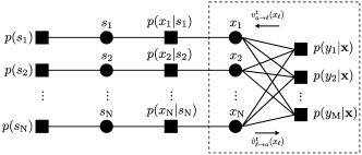
Figure 4: The factor graph of the joint distribution $p(\mathbf{s},\mathbf{x},\mathbf{y}|\mathbf{H}$). Performing sum-product message passing on this factor graph yields the marginal posterior distributions $p(s_{\ell}|\mathbf{y},\mathbf{H})$, $\ell=1,\ldots,N$.

Note that eq:s_hatofv is a one-dimensional integral that can either be evaluated in closed form or via numerical integration as long as the distribution of $\prod_{b=1}^{N}\hat{v}_{b\rightarrow\ell}(x_{\ell})$ is known. To compute the messages $\hat{v}_{b\rightarrow\ell}(x_{\ell})$, we perform message passing on the right side of the factor graph in fig:factorgraph. However, an exact message passing algorithm can quickly result in high complexity; this is mainly because the right side of factor graph in fig:factorgraph is fully connected and we need to compute $2MN$ messages in each iteration. To reduce complexity, we use AMP introduced in [18, 20, 35]. AMP uses the bipartite structure of the graph and the high dimensionality of the problem to approximate the messages with Gaussian distributions. Passing Gaussian messages only requires the message mean and variance instead of PDFs. Furthermore, the structure and dimensionality also allows AMP to approximate all the messages emerging from or going toward one factor node. Specifically, [20, 35] show that all the messages emerging from one factor node have approximately the same value—similarly, all messages going toward the same factor node share approximately the same value. Hence. $v^{t}_{a\rightarrow\ell}\approx v^{t}_{a},\forall\ell=1,\dots,N$ and $\hat{v}^{t}_{i\rightarrow a}\approx\hat{v}^{t}_{i},\forall i=1,\dots,M$. This key observation reduces the number of messages that need to be computed in each iteration from $2MN$ to $M+N$. Reference [4] performs approximate message passing on the system model $\mathbf{y}=\mathbf{H}\mathbf{x}+\mathbf{n}$ with complex entries called cB-AMP (short for complex Bayesian AMP), which calculates an estimate for the effective input signal $\hat{x}_{\ell}$, $\forall\ell$ using the following algorithm.

Algorithm 1 (cB-AMP).

Initialize $\hat{x}^{1}_{\ell}=\operatorname{\mathbb{E}}_{X}[X]$, $\mathbf{r}^{1}=\mathbf{y}$, and $\gamma_{1}^{2}=N_{0}+\beta\operatorname{\mathbb{V}\!\mathrm{ar}}_{X}[X]$ with $X\sim p(x_{\ell})$ as defined in eq:effectiveprior. For $t=1,\ldots,{t_{\textnormal{max}}}$, compute

$$\mathbf{z}^{t} =\hat{}\mathbf{x}^{t}+\mathbf{H}^{\textnormal{H}}\mathbf{r}^{t}$$ (10)

$$\hat{\mathbf{x}}^{t+1} =\mathsf{F}(\mathbf{z}^{t},\gamma_{t}^{2})$$

$$\gamma_{t+1}^{2} =N_{0}+\beta\!\left\langle\mathsf{G}(\mathbf{z}^{t},\gamma_{t}^{2})\right\rangle$$ (11)

$$\mathbf{r}^{t+1} =\textstyle\mathbf{y}-\mathbf{H}\hat{\mathbf{x}}^{t+1}+\beta\frac{\mathbf{r}^{t}}{\gamma_{t}^{2}}\left\langle\mathsf{G}(\mathbf{z}^{t},\gamma_{t}^{2})\right\rangle.$$

The scalar functions $\mathsf{F}(z^{t}_{\ell},\sigma_{t}^{2})$ and $\mathsf{G}(z^{t}_{\ell},\sigma_{t}^{2})$ operate element-wise on vectors, correspond to the posterior mean and variance, respectively, and are defined as follows:

$$\!\!\!\!\mathsf{F}(z^{t}_{\ell},\sigma_{t}^{2}) =\int_{\mathbb{C}}x_{\ell}p(x_{\ell}|z^{t}_{\ell},\sigma_{t}^{2})\mathrm{d}x_{\ell},$$ (12)

$$\!\!\!\!\mathsf{G}(z^{t}_{\ell},\sigma_{t}^{2}) =\int_{\mathbb{C}}\mathopen{}\left\lvert x_{\ell}\right\rvert^{2}\!p(x_{\ell}|z^{t}_{\ell},\sigma_{t}^{2})\mathrm{d}x_{\ell}\!-\!\mathopen{}\left\lvert\mathsf{F}(z^{t}_{\ell},\sigma_{t}^{2})\right\rvert^{2}\!.$$ (13)

The message posterior distribution is $p(x_{\ell}|z^{t}_{\ell},\sigma_{t}^{2})=\frac{1}{Z}p(z^{t}_{\ell}|x_{\ell},\sigma_{t}^{2})p(x_{\ell})$, where $p(z^{t}_{\ell}|x_{\ell},\sigma_{t}^{2})\sim\mathcal{C}\mathcal{N}(x_{\ell},\sigma_{t}^{2})$ and $Z$ is a normalization constant.

As detailed in [4, Sec. III.C], by performing alg:AMP, the so-called Gaussian output $\mathbf{z}^{t}$ of cB-AMP at iteration $t$ in eq:GaussianZ can be modelled in the large system limit as

$$z_{\ell}^{t}=x_{\ell}+w_{\ell}^{t},$$ (14)

with $w_{\ell}^{t}\sim\mathcal{C}\mathcal{N}(0,\sigma^{2}_{t})$, being independent from $x_{\ell}$ (see [19, Sec. 6.4] for details in the real domain). This property is known as the decoupling property as cB-AMP effectively decouples the system into a set of $N$ parallel and independent additive white Gaussian noise (AWGN) channels. Here, $\sigma^{2}_{t}$ is the effective noise variance that can be computed using state evolution, which we introduce in sec:SE. While the quantity $\sigma^{2}_{t}$ cannot be tracked directly within cB-AMP, it can be estimated using the threshold parameter $\gamma^{2}_{t}$ in eq:postulated as shown in [35]. alg:AMP and its Gaussian output $\mathbf{z}^{t}$ are the results of performing AMP on the right side of the factor graph in fig:factorgraph. Next, we will use $\mathbf{z}^{t}$ to perform sum-product message passing on the left side of this factor graph.

II-C AMP with Input Noise (AMPI)

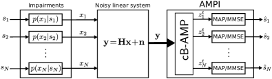
(a) Impaired linear system with AMPI as the estimator.

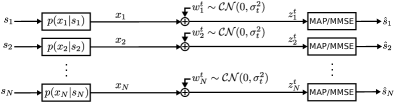
(b) Equivalent decoupled system.

Figure 5: In the large-system limit, AMPI decouples the impaired system into $N$ parallel and independent AWGN channels, which allows us to perform impairment-aware MAP data detection or MMSE estimation.

We now introduce AMPI, the 2-step procedure to recover the input signal $\mathbf{s}$ from the input-output relation illustrated in fig:sysmodel. First, as illustrated in fig:decouple_a, we use cB-AMP in alg:AMP on the effective system model eq:sysmodel to compute the Gaussian output $\mathbf{z}^{t}$ and the effective noise variance $\sigma^{2}_{t}$ at iteration $t$, where the Gaussian output $\mathbf{z}^{t}$ is modelled as in eq:decoupling. fig:decouple_b shows the equivalent input-output relation of the decoupled system. As detailed in the previous section, this is the result of running AMP on the right side of the factor graph in fig:factorgraph. Second, we use sum-product message passing on the left side of factor graph in fig:factorgraph to compute the estimated marginal distribution of $p(s_{\ell}|\mathbf{y,H})$. To compute the marginal, we use the Gaussian output $\mathbf{z}^{t}$ in eq:decoupling, i.e., $p(z_{\ell}^{t}|x_{\ell}^{t})\sim\mathcal{C}\mathcal{N}(x_{\ell}^{t},\sigma^{2}_{t})$; this allows us to compute the marginal posterior distribution for each input signal element $s_{\ell}$ as follows:

$$p(s_{\ell}|\mathbf{y},\mathbf{H}) =p(s_{\ell}|z_{\ell}^{t})\propto p(s_{\ell})p(z_{\ell}^{t}|s_{\ell})$$

$$=p(s_{\ell})\!\int_{\mathbb{C}}p(z_{\ell}^{t}|x_{\ell}^{t})p(x_{\ell}^{t}|s_{\ell})\textnormal{d}x_{\ell}^{t}.$$ (15)

Finally, we can compute individually optimal MAP data detection or MMSE signal estimation for each entry $s_{\ell}$, $\ell=1,\ldots,N$, independently using the marginal distribution. Note that eq:MAP_posterior can be obtained from eq:s_hatofv by computing $\prod_{b=1}^{N}\hat{v}_{b\rightarrow\ell}$. As shown in [20], we have $\prod_{b=1}^{N}\hat{v}_{b\rightarrow\ell}\sim\mathcal{C}\mathcal{N}(z_{\ell}^{t},\sigma^{2}_{t})$. Even though this approach appears to be more straightforward, it lacks the 2-step intuition behind AMPI. The resulting AMPI algorithm is summarized as follows.

Algorithm 2 (AMPI).

Initialize $\hat{x}^{1}_{\ell}=\operatorname{\mathbb{E}}_{X}[X]$, $\mathbf{r}^{1}=\mathbf{y}$, and $\gamma_{1}^{2}=N_{0}+\beta\operatorname{\mathbb{V}\!\mathrm{ar}}_{X}[X]$ with $X\sim p(x_{\ell})$ as in eq:effectiveprior.

1. Run cB-AMP as in alg:AMP for ${t_{\textnormal{max}}}$ iterations.

2. Compute $\hat{s}_{\ell}^{{t_{\textnormal{max}}}}=D(z_{\ell}^{t_{\textnormal{max}}},\sigma^{2}_{t_{\textnormal{max}}})$, where the function $D$ either computes the MAP or MMSE estimate of $s_{\ell}$ using the posterior PDF $p(s_{\ell}|z_{\ell}^{t_{\textnormal{max}}})$ defined in eq:MAP_posterior. The effective noise variance $\sigma^{2}_{t_{\textnormal{max}}}$ is estimated using the threshold parameter $\gamma_{{t_{\textnormal{max}}}}^{2}$ from cB-AMP.

As shown in Sections IV and V, the function $D$ is chosen to satisfy the optimality conditions in eq:IOproblem or eq:MMSEproblem.

II-D Theoretical Analysis of AMPI via State Evolution

Analyzing message passing methods operating on dense graphs is generally difficult. However, the normality of the messages in our application enables us to study theoretical properties in the large-system limit and for uniform linear measurements. As detailed in [35], the effective noise variance $\sigma_{t}^{2}$ of AMP can be calculated analytically for every iteration $t=1,2,\ldots,{t_{\textnormal{max}}}$, using the state evolution recursion.The following theorem repeats the complex state evolution (cSE) for complex AMP (cB-AMP) [4]. In sec:Opt, we will use the cSE framework to derive optimality conditions for AMPI.

Theorem 1.

Assume the model in eq:sysmodel with uniform linear measurements. Run cB-AMP using the function $\mathsf{F}$, where $\mathsf{F}$ is a pseudo-Lipschitz function [37, Sec. 1.1, Eq. 1.5]. Then, in the large-system limit the effective noise variance $\sigma^{2}_{t+1}$ of cB-AMP at iteration $t$ is given by the following cSE recursion:

$$\sigma_{t+1}^{2}=N_{0}+\beta\Psi(\sigma_{t}^{2},\sigma_{t}^{2}),$$ (16)

Here, the MSE function $\Psi$ is defined by

$$\Psi(\sigma_{t}^{2},\gamma_{t}^{2})=\operatorname{\mathbb{E}}_{X,Z}\!\left[\mathopen{}\left\lvert\mathsf{F}\!\left(X+\sigma_{t}Z,\gamma_{t}^{2}\right)-X\right\rvert^{2}\right]$$ (17)

with $X\sim p(x_{\ell})$, $Z\sim\mathcal{C}\mathcal{N}(0,1)$, and $\mathsf{F}$ and $\mathsf{G}$ are the posterior mean and variance functions from alg:AMP. The cSE recursion is initialized at $t=1$ by $\sigma_{1}^{2}=N_{0}+\beta\operatorname{\mathbb{V}\!\mathrm{ar}}_{X}[X]$.

Remark 1.

The posterior mean function $\mathsf{F}$ and the MSE function $\Psi(\sigma_{t}^{2})$ in eq:Psi depend on the effective input signal prior $p(\mathbf{x})$, which, as shown in eq:effectiveprior, is a function of the input signal prior $p(\mathbf{s})$ and the conditional probability $p(\mathbf{x}|\mathbf{s})$ that models the transmit-side impairments. Furthermore, thm:CSE assumes perfect knowledge of the noise variance $N_{0}$; [4, Thm. 1] analyzes the case of a mismatch in the noise variance.

III Optimality of AMPI

We now analyze the optimality of AMPI for the model introduced in sec:intro using the cSE framework.

III-A Optimality of AMPI Within the AMP Framework

In sec:AMPI, we have derived AMPI using message-passing. However, there exists a broader class of algorithms for the same task. Specifically, our version of AMPI performs sum-product message passing using the posterior mean function $\mathsf{F}$ as defined in (12). One can potentially modify $\mathsf{F}$ (or even use different functions at different iterations) to obtain estimates $\hat{x}_{\ell}$, $\ell=1,\ldots,N$, and perform MAP data detection or MMSE estimation on these estimates. Such algorithms can still be analyzed through the state evolution framework. The optimality question we ask here is whether it is possible to improve AMPI by choosing functions different to the ones introduced in (2). As we will show in thm:F_MAPMMSE, the functions we used in first and second step of AMPI algorithm are indeed optimal.

Suppose we run AMPI for ${t_{\textnormal{max}}}$ iterations. Consider a generalization of AMPI, where, in the first step, the posterior mean function $\mathsf{F}$ in eq:Ffunc is replaced with a general pseudo-Lipschitz function $\mathsf{F}_{t}$ that may depend on the iteration index $t$; the MAP or MMSE function in the second is replaced with another function $\mathsf{F}_{{t_{\textnormal{max}}}+1}$. More specifically, we consider

$$\!\!\!\hat{\mathbf{x}}^{t+1}=\textstyle\mathsf{F}_{t}(\mathbf{z}^{t},\gamma_{t}^{2}),\,\,t=1,\dots,{t_{\textnormal{max}}}$$ (18)

$$\!\!\!\hat{\mathbf{s}}\!=\!\textstyle\mathsf{F}_{{t_{\textnormal{max}}}+1}\!(\mathbf{z}^{{t_{\textnormal{max}}}+1}\!,\!\gamma_{{t_{\textnormal{max}}}+1}^{2}),\,\mathbf{z}^{{t_{\textnormal{max}}}+1}\!=\!\hat{}\mathbf{x}^{{t_{\textnormal{max}}}+1}\!\!+\!\mathbf{H}^{\textnormal{H}}\mathbf{r}^{{t_{\textnormal{max}}}+1}\!.$$ (19)

We require the sequence of functions $\{\mathsf{F}_{1},\mathsf{F}_{2},\ldots,\mathsf{F}_{{t_{\textnormal{max}}}+1}\}$ so that thm:CSE holds. Now, the question is whether there exists a sequence of functions $\{\mathsf{F}_{1},\mathsf{F}_{2},\ldots,\mathsf{F}_{{t_{\textnormal{max}}}+1}\}$, such that given the application, the resulting algorithm achieves lower probability of error or lower MSE than AMPI. thm:F_MAPMMSE shows that if the solution to the fixed-point equation of eq:SErecursion is unique, then AMPI is optimal within AMP framework.

The fixed-point equation of eq:SErecursion is computed by letting the number of iterations ${t_{\textnormal{max}}}\to\infty$ in eq:SErecursion, which yields

$$\sigma^{2} =N_{0}+\beta\Psi(\sigma^{2},\sigma^{2}).$$ (20)

Theorem 2.

Assume the system model in sec:intro with uniform linear measurements and the large-system limit. Suppose that we use AMPI with an arbitrary set of pseudo-Lipschitz functions $\mathsf{F}_{1},\ldots,\mathsf{F}_{{t_{\textnormal{max}}}+1}$ as described in eq:generalFs. If the solution to the fixed-point equation in eq:FPsimplified is unique, then the choice of $\mathsf{F}_{1},\ldots,\mathsf{F}_{{t_{\textnormal{max}}}+1}$ that achieves optimal performance according to eq:IOproblem and eq:MMSEproblem are as introduced in alg:AMPI.

thm:F_MAPMMSE shows that it is impossible to improve upon the original choice of AMPI. The proof is given in app:F_MAPMMSE. The fixed-point equation eq:FPsimplified can in general have one or more fixed points. If it has more than one fixed point, then AMPI may converge to different solutions, depending on the initialization [38]. As it is clear from the proof of thm:F_MAPMMSE in app:F_MAPMMSE, even in cases where AMPI does not have a unique fixed point, one of its fixed points corresponds to the optimal solution in AMP framework. Hence, to provide precise conditions for optimality of AMPI, will analyze the fixed point equation eq:FPsimplified for a unique solution only. To establish conditions under which the fixed point equation (20) has a unique solution, we use the following quantities from [5, Defs. 1–4].

Definition 3.

Fix the input signal prior $p(\mathbf{s})$ and input noise distribution $p(\mathbf{x}|\mathbf{s})$. Then, the exact recovery threshold (ERT) $\beta^{\textnormal{max}}$ and the minimum recovery threshold (MRT) $\beta^{\textnormal{min}}$ are

$$\!\beta^{\textnormal{max}}\! =\!\min_{\!\sigma^{2}>0}{\textstyle\!\left\{\!\!\left(\!\frac{\Psi(\sigma^{2},\sigma^{2})}{\sigma^{2}}\!\right)^{\!\!-1}\!\right\}},\,\beta^{\textnormal{min}}\!=\!\min_{\!\sigma^{2}>0}\textstyle\!\left\{\!\!\left(\!\frac{\textnormal{d}\Psi(\sigma^{2},\sigma^{2})}{\textnormal{d}\sigma^{2}}\!\right)^{\!\!-1}\!\right\}\!.$$ (21)

The minimum critical noise $N_{0}^{\textnormal{min}}(\beta)$ is defined as

$$N_{0}^{\textnormal{min}}(\beta) =\min_{\sigma^{2}>0}\textstyle\!\left\{\sigma^{2}-\beta\Psi(\sigma^{2},\sigma^{2}):\beta\frac{\textnormal{d}\Psi(\sigma^{2},\sigma^{2})}{\textnormal{d}\sigma^{2}}=1\right\}\!,$$ (22)

and the maximum guaranteed noise $N_{0}^{\textnormal{max}}(\beta)$ is defined as

$$N_{0}^{\textnormal{max}}(\beta) =\max_{\sigma^{2}>0}\textstyle\!\left\{\sigma^{2}-\beta\Psi(\sigma^{2},\sigma^{2}):\beta\frac{\textnormal{d}\Psi(\sigma^{2},\sigma^{2})}{\textnormal{d}\sigma^{2}}=1\right\}\!.$$ (23)

Using def:betaN0, the following theorem establishes three regimes for which fixed-point equation eq:FPsimplified has an unique solution. The proof follows from [4, Sec. IV-D, IV-E].

Lemma 3.

Let the assumptions of thm:CSE hold and ${t_{\textnormal{max}}}\to\infty$. Fix $p(\mathbf{s})$ and $p(\mathbf{x}|\mathbf{s})$. If the variance of the receive noise $N_{0}$ and system ratio $\beta$ are in one of the following three regimes:

1. $\beta\in\left(0,\beta^{\textnormal{min}}\right]$ and $N_{0}\in\mathbb{R}^{+}$

2. $\beta\in\left(\beta^{\textnormal{min}},\beta^{\textnormal{max}}\right)$ and $N_{0}\in\left[0,N_{0}^{\textnormal{min}}(\beta)\right)\cup\left(N_{0}^{\textnormal{max}}(\beta),\infty\right)$

3. $\beta\in\left[\beta^{\textnormal{max}},\infty\right)$ and $N_{0}\in\left(N_{0}^{\textnormal{max}}(\beta),\infty\right)$,

then the fixed point equation eq:FPsimplified has a unique solution.

For AMPI, the quantities in def:betaN0 depend on $p(\mathbf{x})$, which is a function of $p(\mathbf{s})$ and $p(\mathbf{x}|\mathbf{s})$ (cf. rem:dependence). These quantities can be computed either numerically or in closed-form (see [5, Sec. III]). In many applications, the effective input signal prior $p(\mathbf{x})$ is continuous and bounded which results in certain properties for ERT and MRT as discussed in the following lemma. The proof is given in app:betalimits.

Lemma 4.

Suppose the probability density $p(\mathbf{x})$ of the effective input signal $\mathbf{x}$ is continuous and bounded. Furthermore, let the assumptions made in thm:CSE hold. Then, the ERT and MRT satisfy $\beta^{\textnormal{max}}=1$ and $\beta^{\textnormal{min}}\leq 1$.

From lem:betalimits, we conclude that for a system with a continuous effective input signal prior $p(\mathbf{x})$ we have $\beta^{\textnormal{min}}\leq 1$. As noted in lem:betaN0, $\beta^{\textnormal{min}}$ determines the values of system ratio $\beta$ under which AMPI can be optimal for any noise variance. In other words, $\beta\leq\beta^{\textnormal{min}}\leq 1$ implies that the system should not be under-determined. As an example, consider a massive MIMO system that uses QPSK constellations. In the absence of input noise, $\beta^{\textnormal{min}}\approx 2.9505$ (see [5, Tbl. I]). However, by adding the slightest amount of input noise with a continuous probability distribution, such as Gaussian input noise, $\beta^{\textnormal{min}}$ abruptly decreases to values no larger than $1$.

IV Application 1: Massive MIMO

As discussed in sec:intro, impairment-aware data detection is an important part of practical massive MIMO systems. In reference [1], we provided an impairment-aware data detection algorithm called LAMA-I (short for large-MIMO approximate message passing with transmit impairments). LAMA-I which is a low-complexity data detection algorithm, is AMPI derived for massive MIMO systems. In this section, we briefly revisit the signal and system model for massive MIMO and LAMA-I from [1]. We then provide an optimality analysis of LAMA-I which was not shown in [1]. In particular, we prove that besides optimality in the AMP framework, LAMA-I is able to achieve the same error-rate performance as the IO data detector.

IV-A LAMA-I: AMPI for Massive MIMO Data Detection

Consider an input signal $\mathbf{s}\in\mathbb{C}^{N}$ sent through an impaired MIMO channel with input-output relation eq:sysmodel introduced in sec:intro with the following assumptions. The entries of $\mathbf{s}$ are chosen from a constellation set $\mathcal{O}$, e.g., QAM, and $\mathbf{s}$ is assumed to have i.i.d. prior distribution $p(\mathbf{s})=\prod_{\ell=1}^{N}p(s_{\ell})$ with the following distribution for each transmit symbol:

$$p\!\left(s_{\ell}\right)=\sum_{a\in\mathcal{O}}p_{a}\delta\!\left(s_{\ell}-a\right)\!.$$ (24)

The received vector is $\mathbf{y}\in\mathbb{C}^{M}$ is the received vector, and $N$ and $M$ denote the number of user equipments and base-station antennas, respectively. The MIMO channel matrix $\mathbf{H}\in\mathbb{C}^{M\times N}$ is assumed to be perfectly known at the receiver.

As shown in alg:AMPI, we first use cB-AMP to compute the Gaussian output $\mathbf{z}^{{t_{\textnormal{max}}}}$ and the effective noise variance $\sigma^{2}_{{t_{\textnormal{max}}}}=\gamma^{2}_{{t_{\textnormal{max}}}}$ at iteration $t$. The MIMO system is decoupled into a set of $N$ parallel and independent additive white Gaussian noise (AWGN) channels. fig:decouple_b shows the equivalent decoupled system. Using eq:MAP_posterior, we can compute the marginal posterior distribution $p(s_{\ell}|\mathbf{y},\mathbf{H})=p(s_{\ell}|z_{\ell}^{{t_{\textnormal{max}}}})$ from the Gaussian output. The marginal posterior distribution allows us to compute the MAP estimate for each data symbol independently as

$$\hat{s}_{\ell}^{{t_{\textnormal{max}}}}=D(z_{\ell}^{t_{\textnormal{max}}},\sigma^{2}_{t_{\textnormal{max}}})=\operatorname*{arg\;max}_{s_{\ell}\in\mathcal{O}}p(s_{\ell}|z_{\ell}^{{t_{\textnormal{max}}}}).$$ (25)

We call this procedure the LAMA-I algorithm in [1]. Note that [1, Sec. IV] details the derivation of LAMA-I for a Gaussian input noise model $p(x_{\ell}|s_{\ell})=\mathcal{C}\mathcal{N}(s_{\ell},N_{\textnormal{T}}),\forall\ell={1,\ldots,N}$.

IV-B Individually Optimal (IO) Data Detection

We now show that for uniform linear measurements and the large-system limit, LAMA-I is able to achieve the error-rate performance of the IO data detector eq:IOproblem, if the fixed-point equation eq:FPsimplified has a unique solution. There has been some work in the past focusing on optimality of AMP in the absence of input noise such as [39] (see [4, Sec. IV] for a survey). The core of our optimality analysis is the performance of IO data detection in the presence of input noise based on the replica analysis presented in [40]. To prove individual optimality, we first introduce the following definition. The replica analysis for IO data detection makes the following assumption about $\hat{s}^{\textnormal{IO}}_{\ell}$.

Definition 4.

The IO solution $\hat{s}^{\textnormal{IO}}_{\ell}$ is said to satisfy hard-soft assumption, if and only if there exist a function $D:\mathbb{R}\rightarrow\mathcal{O}$, with the following properties: (i) $\hat{s}^{\textnormal{IO}}_{\ell}=D(\mathbb{E}(s_{\ell}|\mathbf{y,H}))$ and (ii) for every $s\in\mathcal{O}$ the $D^{-1}(s)$ is Borel measurable and its boundary has Lebesgue measure zero.

We can prove that the hard-soft assumption is in fact true for equiprobable BPSK constellation points, i.e., we have

$$\mathbb{E}({s}_{\ell}|\mathbf{y,H})=\mathbb{P}({s}_{\ell}=+1|\mathbf{y,H})-\mathbb{P}({s}_{\ell}=-1|\mathbf{y,H}),$$

and hence, $\hat{s}^{\textnormal{IO}}_{\ell}=\operatorname{sign}(\mathbb{E}({s}_{\ell}|\mathbf{y,H}))$. However, it is an interesting open problem whether the assumption in def:hardsoft holds for other, more general, constellations as well.

To simplify our proofs, we make an extra assumption:

Definition 5.

The IO solution $\hat{s}^{\textnormal{IO}}_{\ell}$ is said to satisfy the fixed-D assumption, if in addition to satisfying the hard-soft assumption, the function $D$ from def:hardsoft is only a function of $\beta$, $p(s_{\ell})$, $p(x_{\ell}|s_{\ell})$, and $p(n_{\ell})$. In particular, $D$ does not depend on the dimension $N$ of the input signal.

Note that for equiprobable BPSK symbols, we have $\hat{s}^{\textnormal{IO}}_{\ell}=\operatorname{sign}(\mathbb{E}({s}_{\ell}|\mathbf{y,H}))$ and the fixed-D assumption clearly holds. Intuitively speaking, when the dimensions are large, we do not expect the function $D$ to change with the dimension $N$.

Before we can establish individual optimality of LAMA-I, we introduce thm:IOfixedD, which analyzes the error probability of the IO solution and provides an equivalent relation, which enables us to compute the error probability of an IO data detector and consequently compare it with other detectors.

Theorem 5.

Suppose that the IO solution satisfies both the hard-soft and fixed-D assumptions in Definitions 4 and 5. Furthermore, assume that the assumptions underlying the replica symmetry in [40] are correct. Then, $\mathbb{P}(\hat{s}^{\textnormal{IO}}_{\ell}\neq s_{\ell})$ converges to $\mathbb{P}(D(Q)\neq S)$ in probability. Here $Q=X+\tilde{\sigma}Z$ with $p(S,X)=p(s_{\ell})p(x_{\ell}|s_{\ell})$, $Z\sim\mathcal{C}\mathcal{N}(0,1)$ being independent of $(S,X)$ and $\tilde{\sigma}$ satisfying the following equation:

$$\tilde{\sigma}^{2}=N_{0}+\beta\Psi(\tilde{\sigma}^{2}).$$ (26)

We now provide conditions for which LAMA-I algorithm achieves the error-rate performance of IO data detector. The proof is given in app:IOptimality.

Theorem 6.

Assume the system model in eq:sysmodel with uniform linear measurements. Suppose that the assumptions made in thm:IOfixedD hold. Furthermore, assume that the fixed-point equation (26) has a unique solution. Let us call the estimate of LAMA-I after $t$ iterations $\hat{s}_{\ell}^{t}$. Then in large-system limit, for any $\epsilon\geq 0$ there exists an iteration number $t_{0}$ such that

$$\lim_{N\rightarrow\infty}\frac{1}{N}\sum_{\ell=1}^{N}\mathbb{P}(\hat{s}_{\ell}^{t_{0}}\neq s_{\ell})\leq\lim_{N\rightarrow\infty}\frac{1}{N}\sum_{\ell=1}^{N}\mathbb{P}(\hat{s}_{\ell}^{\textnormal{IO}}\neq s_{\ell})+\epsilon,$$

where the limits are taken in probability.

thm:IOptimality proves individual optimality of LAMA-I algorithm given certain conditions are met on system size and ratio. The inequality in this theorem shows how LAMA-I with an infinite number of iterations achieves the same error-rate as that of IO data detector. While LAMA-I requires the large-system limit and an infinite number of iterations to achieve the performance of IO data detector, fig:MIMO and simulation results in [1] demonstrate that LAMA-I achieves near-IO performance in realistic, finite dimensional large-MIMO systems.

V Application 2: Compressive Sensing

We now apply AMPI to compressive sensing signal recovery in the presence of input noise. We first introduce the system model and then derive AMPI for this system. We conclude with simulation results that compare AMPI to existing methods.

V-A System Model

The noiseless version of CS signal recovery can be solved perfectly under certain conditions on the system dimension and the sparsity level [11, 18]. Recovery under measurement noise has been analyzed extensively; see, e.g., [19, 41]. However, practical CS systems may be affected by input noise [15, 14]. For example, the input signals may not be perfectly sparse or might be affected by noise that appears prior to the measurement process. In what follows, we introduce AMPI to recover the sparse input signal from measurements contaminated with both input and measurement noise. Let $\mathbf{s}\in\mathbb{R}^{N}$ be the signal of interest we want to reconstruct from the noisy measurements $\mathbf{y}\in\mathbb{R}^{M}$ with the system model in eq:sysmodel introduced in sec:intro. Since the system model for compressive sensing is assumed to be under-determined, we have $M\leq N$ (or equivalently $\beta\geq 1$). Moreover, the input signal $\mathbf{s}$ is a sparse vector with at most $K$ non-zero entries.

V-B AMPI for Compressive Sensing

To apply alg:AMPI for CS, we first need to derive the effective input signal prior $p(\mathbf{x})$ in eq:effectiveprior, which requires the input signal prior $p(\mathbf{s})$. As explained in [19], a practical solution to capture sparsity in $\mathbf{s}$ is to assume an i.i.d. Laplace prior. We assume $p(\mathbf{s})=\left(\frac{\lambda}{2}\right)^{N}\exp\left(-\lambda\|\mathbf{s}\|_{1}\right)$ with a regularization parameter $\lambda>0$ that can be tuned to best model the sparsity of the input signal $\mathbf{s}$. For optimal performance, one should tune $\lambda$ to minimize the MSE of AMPI. Besides the parameter $\lambda$, AMPI requires a threshold parameter $\gamma_{t}^{2}$ that must be tuned in each iteration. To attain optimal performance, both of these parameters should be tuned in each algorithm iteration. To this end, we will use an iteration index subscript for $\gamma_{t}^{2}$ and for $\lambda_{t}$.

As noted in sec:path-AMPI, there exist different methods to tune the threshold parameter $\gamma_{t}^{2}$. In the paper [42], the authors propose an asymptotically optimal tuning approach using Stein’s unbiased risk estimate (SURE) [43] for the threshold parameter $\gamma_{t}^{2}$. Here, we follow a similar approach that optimally tunes both parameters $\lambda_{t}$ and $\gamma_{t}^{2}$.

First, run Step 1 of alg:AMPI for ${t_{\textnormal{max}}}$ iterations. Optimal tuning for AMPI can be achieved if $\lambda_{1},\dots,\lambda_{{t_{\textnormal{max}}}}$ and $\gamma_{1}^{2},\dots,\gamma_{{t_{\textnormal{max}}}}^{2}$ are tuned in such a way that the value of the asymptotic MSE or $\!\!\lim\limits_{N\to\infty}\frac{1}{N}\|\hat{\mathbf{x}}^{{t_{\textnormal{max}}}+1}\!-\mathbf{x}\|^{2}$ is minimized. This requires a joint optimization of the asymptotic MSE over all variables $\{\lambda_{1},\dots,\lambda_{{t_{\textnormal{max}}}},\gamma_{1}^{2},\dots,\gamma_{{t_{\textnormal{max}}}}^{2}\}$. However, such a joint optimization is not practical as the iterative nature of AMPI does not allow one to write an explicit expression for MSE. The following theorem shows that one can simplify the joint parameter optimization by tuning each pair $(\lambda_{t},\gamma_{t}^{2})$ at iteration $t$ starting from $t=1$ to ${t_{\textnormal{max}}}$. The proof for this theorem follows from [42, Thm. 3.7] with minor modifications.

Theorem 7.

Suppose that the parameters $\lambda_{1}^{,}\dots,\lambda_{{t_{\textnormal{max}}}}^{,},$ $\gamma_{1}^{2},\dots,\gamma_{{t_{\textnormal{max}}}}^{2}$ are optimally tuned for iteration ${t_{\textnormal{max}}}$ of AMPI. Then, $\forall t<{t_{\textnormal{max}}}$, the parameters $\lambda_{1},\dots,\lambda_{t},\gamma_{1}^{2},\dots,\gamma_{t}^{2}$ are also optimally tuned for iteration $t$.

thm:opt-tuning implies that instead of jointly tuning all parameters $\{\lambda_{1},\dots,\lambda_{{t_{\textnormal{max}}}},\gamma_{1}^{2},\dots,\gamma_{{t_{\textnormal{max}}}}^{2}\}$, we can tune $(\lambda_{1},\gamma_{1}^{2})$ at iteration 1. Given the parameters $(\lambda_{1},\gamma_{1}^{2})$, we can then tune $(\lambda_{2},\gamma_{2}^{2})$ at iteration 2, and repeat this process for ${t_{\textnormal{max}}}$ iterations.

The missing piece is to minimize the MSE at iteration $t$ with appropriate parameters $(\lambda_{t},\gamma_{t}^{2})$. As cSE in thm:CSE suggest, the asymptotic MSE at iteration $t$ is given by the function $\Psi(\sigma_{t}^{2},\gamma_{t}^{2},\lambda_{t})=\operatorname{\mathbb{E}}_{X,Z}\!\left[\mathopen{}\left\lvert\mathsf{F}\!\left(X+\sigma_{t}Z,\gamma_{t}^{2},\lambda_{t}\right)-X\right\rvert^{2}\right]$, with $X\sim p(x_{\ell})$, $Z\sim\mathcal{C}\mathcal{N}(0,1)$, and $\mathsf{F}$ as the posterior mean function introduced in eq:Ffunc. Notice that all functions $\Psi$, $\mathsf{F}$, and $\mathsf{G}$ will also be a function of $\lambda_{t}$. We use a similar tuning approach as in [42] and since the MSE function $\Psi(\sigma_{t}^{2},\gamma_{t}^{2},\lambda_{t})$ depends on the unknown signal prior $p(X)$, we estimate it using SURE in each iteration. For AMPI, SURE is given by

$$\hat{\Psi}(\sigma_{t}^{2},\lambda_{t},\gamma_{t}^{2})=\, \textstyle\frac{1}{N}\|\mathsf{F}(\mathbf{z}^{t},\gamma_{t}^{2},\lambda_{t})-\mathbf{z}^{t}\|^{2}+\sigma_{t}^{2}$$

$$\textstyle+\frac{2\sigma_{t}^{2}}{\gamma_{t}^{2}}\left\langle\mathsf{G}(\mathbf{z}^{t},\gamma_{t}^{2},\lambda_{t})-1\right\rangle,$$ (27)

where we estimate $\sigma_{t}^{2}$ by ${\|\mathbf{r}^{t}\|^{2}}/{M}$ as in [19]. We now modify AMPI as in alg:AMPI for CS applications as follows.

Algorithm 3 (AMPI-SURE).

Set $\hat{\mathbf{x}}^{1}=0$ and $\mathbf{r}^{1}=\mathbf{y}$.

1. For $t=1,2,\ldots,{t_{\textnormal{max}}}$ compute

   $$\mathbf{z}^{t} =\hat{}\mathbf{x}^{t}+\mathbf{H}^{\textnormal{H}}\mathbf{r}^{t}$$

   $$(\lambda_{t},\gamma_{t}^{2}) =\operatorname*{arg\;min}\limits_{\lambda\geq 0,\gamma^{2}\geq 0}\hat{\Psi}(\sigma_{t}^{2},\lambda,\gamma^{2})$$

   $$\hat{\mathbf{x}}^{t+1} =\mathsf{F}(\mathbf{z}^{t},\gamma_{t}^{2},\lambda_{t})$$

   $$\mathbf{r}^{t+1} =\textstyle\mathbf{y}-\mathbf{H}\hat{\mathbf{x}}^{t+1}+\beta\frac{\mathbf{r}^{t}}{\gamma_{t}^{2}}\left\langle\mathsf{G}(\mathbf{z}^{t},\gamma_{t}^{2},\lambda_{t})\right\rangle.$$

   Here, $\hat{\Psi}$ is given by eq:Psihat, and $\mathsf{F}$ and $\mathsf{G}$ are the posterior mean and variance given by eq:Ffunc, where $p(x_{\ell})=\int_{\mathbb{C}}p(x_{\ell}|s_{\ell})p(s_{\ell})\textnormal{d}s_{\ell}$ and $p(s_{\ell})=\frac{\lambda_{t}}{2}\exp\left(-\lambda_{t}|s_{\ell}|\right)$.

2. Compute the MMSE estimate for $t={t_{\textnormal{max}}}$ with the posterior PDF $p(s_{\ell}|z_{\ell}^{t_{\textnormal{max}}})$ as defined in eq:MAP_posterior and $p(w_{\ell}^{t_{\textnormal{max}}})\sim\mathcal{N}(0,\sigma^{2}_{t_{\textnormal{max}}})$. The effective noise variance $\sigma^{2}_{t_{\textnormal{max}}}$ and signal prior distribution $p(s_{\ell})$ are estimated using $\gamma_{{t_{\textnormal{max}}}}^{2}$ and $\frac{\lambda_{{t_{\textnormal{max}}}}^{*}}{2}\exp\!\left(-\lambda_{{t_{\textnormal{max}}}}^{*}\|\,\mathrm{s}_{\ell}\|_{1}\right)$.

alg:AMPI-SURE summarizes AMPI for CS. The only difference to alg:AMPI is the presence of the extra parameter $\lambda_{t}$ that is optimally tuned using SURE depending on the signal sparsity.

V-C AMPI Sparse Signal Recovery Under Gaussian Input Noise

AMPI for CS recovery as in alg:AMPI-SURE is defined for a general class of input noise distributions $p(\mathbf{x}|\mathbf{s})$. We now provide a derivation of AMPI for the specific case of Gaussian input noise, i.e., where $p(\mathbf{x}|\mathbf{s})=\mathcal{C}\mathcal{N}(\mathbf{s},N_{\textnormal{T}}\mathbf{I}_{M})$ [14, 15]. The following lemma details the prior $p(\mathbf{x})$ and the functions $\mathsf{F}$ and $\mathsf{G}$ needed in Steps 1 and 2 of alg:AMPI-SURE. The derivations are given in app:FG_CS in supplementary.

Lemma 8.

For a CS system as defined by sec:CS_model, the prior $p(\mathbf{x})$, the posterior mean $\mathsf{F}$ and variance $\mathsf{G}$ defined in alg:AMPI-SURE are given by:

$$p(\mathbf{x}) =\prod\limits_{i=1}^{N}\frac{\lambda}{2}\exp\!\left(\frac{\lambda^{2}N_{\textnormal{T}}}{2}\right)\!\bigg{(}\!\exp(\lambda x_{i})Q\!\left(\frac{x_{i}+\lambda N_{\textnormal{T}}}{\sqrt{N_{\textnormal{T}}}}\right)\!$$

$$\quad+\exp(-\lambda x_{i})\!\left(1-Q\!\left(\frac{x_{i}-\lambda N_{\textnormal{T}}}{\sqrt{N_{\textnormal{T}}}}\right)\right)\!\bigg{)}$$ (28)

$$\mathsf{F}(\hat{x},\tau,\lambda) =\hat{x}+\lambda\tau\eta(\hat{x},\tau)$$ (29)

$$\mathsf{G}(\hat{x},\tau,\lambda) =\tau+\lambda^{2}\tau^{2}(1-(\eta(\hat{x},\tau))^{2})$$

$$\quad-\frac{4}{\gamma(\hat{x},\tau)}\frac{\lambda\tau^{2}}{\sqrt{2\pi(N_{\textnormal{T}}+\tau)}},$$ (30)

where we define

$$\eta(\hat{x},\tau) =\frac{\mathrm{erfcx}(\alpha)-\mathrm{erfcx}(\beta)}{\mathrm{erfcx}(\alpha)+\mathrm{erfcx}(\beta)}$$ (31)

$$\gamma(\hat{x},\tau) =\mathrm{erfcx}(\alpha)+\mathrm{erfcx}(\beta)$$ (32)

$$\alpha =\frac{\hat{x}+\lambda(N_{\textnormal{T}}+\tau)}{\sqrt{2(N_{\textnormal{T}}+\tau)}}$$ (33)

$$\beta =\frac{-\hat{x}+\lambda(N_{\textnormal{T}}+\tau)}{\sqrt{2(N_{\textnormal{T}}+\tau)}}.$$ (34)

The Q-function is $Q(x)=\int_{x}^{\infty}\frac{1}{\sqrt{2\pi}}\exp\left(\!-\frac{t^{2}}{2}\right)\textnormal{d}t$, the error function $\mathrm{erfc}(x)=2Q(\sqrt{2}x)$, and $\mathrm{erfcx}(x)=x^{2}\mathrm{erfc}(x)$.

Before providing simulation results for AMPI-SURE, we next summarize two baseline algorithms used as a comparison.

V-D Two Alternative Algorithms

V-D1 Noise Whitening

Noise whitening has been proposed for data detection and compressive sensing in [8] and [15], respectively. This approach relies on the Gaussian input-noise model, which enables one to “whiten” the impaired system model eq:sysmodel by multiplying the vector $\mathbf{y}$ with the whitening matrix $\mathbf{W}=N_{0}\mathbf{Q}^{-\frac{1}{2}}$, where $\mathbf{Q}=N_{\textnormal{T}}\mathbf{H}\mathbf{H}^{\textnormal{H}}+N_{0}\mathbf{I}_{M}$ is the covariance matrix of the effective input and receive noise $\mathbf{n}+\mathbf{H}\mathbf{e}$. Whitening resultsin a statistically equivalent input-output relation $\tilde{\mathbf{y}}=\tilde{\mathbf{H}}\mathbf{s}+\tilde{\mathbf{n}}$, where $\tilde{\mathbf{y}}=\mathbf{W}\mathbf{y}$, $\tilde{\mathbf{H}}=\mathbf{W}\mathbf{H}$ and $\tilde{\mathbf{n}}\sim\mathcal{C}\mathcal{N}(0,N_{0}\mathbf{I}_{M})$ is independent of $\mathbf{s}$ [8]. Thus, signal recovery can be performed with conventional algorithms, such as AMP [21, 22]. The drawback of noise whitening is in computing the whitening matrix $\mathbf{W}$, whose dimensions may be extremely large (e.g., in imaging applications). AMPI avoids computation of $\mathbf{W}$, which reduces complexity. Furthermore, AMPI supports more general input noise models—in contrast, noise whitening requires a Gaussian input-noise model.

V-D2 Convex Optimization

Consider the system model in sec:CS_model. If the input noise is zero, i.e. $\mathbf{x}=\mathbf{s}$, then for a sparse signal $\mathbf{s}$ or equivalently $\mathbf{x}$, sparse signal recovery can be performed by solving [35]

$$\hat{\mathbf{s}}=\operatorname*{arg\;min}_{\mathbf{s}}\textstyle\frac{1}{2}\|\mathbf{y}-\mathbf{H}\mathbf{s}\|^{2}_{2}+\lambda\|\mathbf{s}\|_{1}.$$

If the input noise is non-zero, i.e., $\mathbf{x}\neq\mathbf{s}$, then we can solve the following optimization problem:

$$\hat{}\mathbf{x}=\operatorname*{arg\;min}_{\mathbf{x}}\frac{1}{2N_{0}}\|\mathbf{y}-\mathbf{H}\mathbf{x}\|_{2}^{2}-\log p(\mathbf{x})$$ (35)

If the term $-\log p(\mathbf{x})$ is convex and differentiable, then we can use efficient algorithms that guarantee convergence to an optimal solution. The following result establishes convexity for the Gaussian input-noise model and provides the gradient, which we use to solve eq:CS_ConvexProblem. The proof is given in app:CS_convexity in supplementary derivations.

Lemma 9.

The objective function $q(\mathbf{x})=\frac{1}{2N_{0}}\|\mathbf{y}-\mathbf{H}\mathbf{x}\|_{2}^{2}-\log p(\mathbf{x})$ is convex and its gradient is given by

$$\nabla_{\mathbf{x}}q(\mathbf{x})=\frac{1}{N_{0}}(\mathbf{H}\mathbf{x}-\mathbf{y})^{\textnormal{T}}\mathbf{H}-\nabla_{\mathbf{x}}\left[\log p(\mathbf{x})\right]\!,$$ (36)

and, $\!\nabla_{\mathbf{x}}\!\left[\log p(\mathbf{x})\right]\!\!=\!\!\lambda[\eta(x_{1},\!0),...,\!\eta(x_{N},\!0)]^{\textnormal{T}}$ with $\eta(\hat{x},\!\tau\!)$ in eq:eta.

Hence, we propose to use the non-linear conjugate gradient method of Polak-Ribiere [44] to solve for eq:CS_ConvexProblem; see [45, alg. 4.4] for the algorithm details. The downside of such an approach is that there is no known fast approach to set the parameter $\lambda$. In contrast, AMPI in alg:AMPI-SURE can be tuned optimally.

V-E Results and Comparison

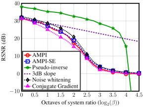
Figure 6: Reconstruction SNR of AMPI and other algorithms for sparse signal recovery with input noise. The signal has sparsity of $5\%$, SNR of $30$ dB, and is affected by input noise with EVM of $-30$ dB. AMPI achieves the same performance as noise whitening and nonlinear conjugate gradients but at much lower computational complexity.

fig:RSNRcomp shows simulation results for sparse signal recovery with a sparsity rate of $\frac{K}{N}=5\%$ and signal dimension of $N=1000$. The input signal is generated with a Bernoulli-Gaussian distribution. The indices of the non-zeros entries are selected from an equiprobable Bernoulli distribution and each entry is generated from a standard normal distribution. The reconstruction signal to noise ratio (RSNR) is plotted as a function of the octaves of system ratio $\beta$ (also referred to as sub-sampling ratio). Furthermore, we consider an average SNR of $\textit{SNR}={\operatorname{\mathbb{E}}\left[\|\mathbf{H}\mathbf{s}\|^{2}\right]}/{\operatorname{\mathbb{E}}\left[\|\mathbf{n}\|^{2}\right]}=\beta\frac{E_{s}}{N_{0}}=30$ dB and an error vector magnitude of $\textit{EVM}={\operatorname{\mathbb{E}}\left[\|\mathbf{e}\|^{2}\right]}/{\operatorname{\mathbb{E}}\left[\|\mathbf{s}\|^{2}\right]}=\frac{N_{\textnormal{T}}}{E_{s}}=-30$ dB. In fig:RSNRcomp, the RSNR results of each algorithm is averaged over 20 different randomly-created input signals. The performance of AMPI with 100 iterations is depicted as a solid circle-marked red curve. AMPI’s performance almost perfectly matches the cSE predictions in eq:SErecursion (the dashed square-marked blue curve). As a comparison, we show the performance of noise whitening and convex optimization with non-linear conjugate gradients. The dotted diamond-marked black curve shows the performance of noise whitening followed by AMP. While whitening achieves the same performance as AMPI, it entails significantly higher complexity as one has to first compute the whitening matrix. The dotted triangle-marked magenta curve shows the performance of nonlinear conjugate gradients with $100$ iterations. This method requires a computationally expensive grid search per each iteration to tune the parameter $\lambda$. Since we set this tuning parameter using the optimal ones from AMPI (solid circle-marked red curve), the conjugate gradients method performs very well. The solid star-marked green curve corresponds to the oracle-based approach of taking the pseudo-inverse assuming the support is known. As [13] suggests, the RSNR of this method decays with a slope of $3$ dB per octave. However, none of the proposed algorithms follows the $3$dB per octave slope.

VI Conclusion

We have introduced AMPI (short for approximate message passing with input noise), a novel data detection and estimation algorithm for systems that are corrupted by input noise. AMPI is computationally efficient and can be used for a broad range of input-noise models. Furthermore, the complex state-evolution (cSE) framework enables a theoretical analysis of AMPI in the large system limit and for i.i.d. Gaussian measurement matrices. Under these conditions, we have investigated optimality conditions of AMPI for data detection and signal estimation. We have shown that AMPI is optimal within the AMP framework and, under additional assumptions, achieves individually-optimal error-rate performance in massive MIMO applications. For the Gaussian input-noise model, we have used numerical results to show that AMPI outperforms methods that ignore input noise and performs on-par with whitening and optimization-based methods, but at (often significantly) lower complexity.

Appendix A Proof of thm:F_MAPMMSE

A-A Proof Outline

We provide an optimality proof for an application where AMPI solves the IO problem in eq:IOproblem. This means that in Step 2 of AMPI, we use the MAP estimate. The optimality proof where AMPI is supposed to minimize the MSE follows analogously. Suppose that we use AMPI with an arbitrary set of pseudo-Lipschitz functions $\mathsf{F}_{1},...,\mathsf{F}_{{t_{\textnormal{max}}}+1}$ as described in eq:generalFs. In this proof, we will establish that AMPI in alg:AMPI chooses these functions such that the outputs $\hat{s}_{\ell}$ for $\ell\!=\!1,...,N$, correspond to the solution of the IO problem eq:IOproblem in the large-system limit. We start by writing down the optimality criterion in eq:IOproblem as

$$\mathsf{F}_{\!{t_{\textnormal{max}}}\!+\!1}\!(\!z_{\ell}^{{t_{\textnormal{max}}}+1}\!\!,\!\sigma_{{t_{\textnormal{max}}}+1}^{2}\!)\!=\!\operatorname*{arg\;min}\limits_{\mathsf{F}}\mathbb{P}\!\left(\!\mathsf{F}(z_{\ell}^{{t_{\textnormal{max}}}\!+\!1}\!\!,\!\sigma_{{t_{\textnormal{max}}}\!+\!1}^{2})\!\neq\!s_{\ell}\!\right)\!\!.$$ (37)

The estimate generated by the function $\mathsf{F}_{{t_{\textnormal{max}}}+1}(z^{{t_{\textnormal{max}}}+1}_{\ell},\sigma_{{t_{\textnormal{max}}}+1}^{2})$ during Step 2 at iteration ${{t_{\textnormal{max}}}+1}$ minimizes the per-entry symbol-error probability. Note that the functions $\mathsf{F}_{1},\ldots,\mathsf{F}_{{t_{\textnormal{max}}}+1}$ operate element-wise on vectors.

Remark 2.

The criterion eq:Opt_criterion appears to only consider the $\ell$th entry. Since, however, the probability in eq:Opt_criterion is taken w.r.t. the randomness in the matrix $\mathbf{H}$, the vector $\mathbf{s}$, input and receive noise, the criterion is in fact affected by all other entries.

We now establish the optimality proof by the following two lemmas, with proofs in app:FMAP and A-C. In what follows, we assume the random variables $S\sim p(s_{\ell}),X|S\sim p(x_{\ell}|s_{\ell})$, and $Z\sim\mathcal{C}\mathcal{N}(0,1)$ to be independent of $X$ and $S$.

Lemma 10.

Let the assumptions of Thm. 2 hold. For the criterion eq:Opt_criterion to hold for $\ell=1,\ldots,N$, $\mathsf{F}_{{t_{\textnormal{max}}}+1}(z^{{t_{\textnormal{max}}}+1}_{\ell},\sigma_{{t_{\textnormal{max}}}+1}^{2})$ at iteration ${t_{\textnormal{max}}}+1$ must be the MAP estimator

$$\mathsf{F}_{\!{t_{\textnormal{max}}}\!+\!1\!}(\!z^{{t_{\textnormal{max}}}\!+\!1}_{\ell}\!\!,\!\sigma_{{t_{\textnormal{max}}}\!+\!1}^{2}\!)\!=\!\operatorname*{arg\;max}\limits_{s_{\ell}\in\mathcal{O}}{p_{S|X+\sigma_{{t_{\textnormal{max}}}\!+\!1}\!Z}(\!s_{\ell}|z_{\ell}^{{t_{\textnormal{max}}}+1}\!)}$$ (38)

Lemma 11.

Let the assumptions of Thm. 2 hold. For the criterion eq:Opt_criterion to hold for $\ell=1,\ldots,N$, the functions $\mathsf{F}_{t}(z^{t}_{\ell},\sigma_{t}^{2})$, $t=1,\ldots,{{t_{\textnormal{max}}}}$, must be the unique set of MMSE estimators, i.e., $\mathsf{F}_{t}(z^{t}_{\ell},\sigma_{t}^{2})=\operatorname{\mathbb{E}}_{X|X+\sigma_{t}Z}[x_{\ell}|z_{\ell}^{t}]$.

lem:FMAP suggests that for optimality to hold, the function $\mathsf{F}_{{t_{\textnormal{max}}}+1}(z^{{t_{\textnormal{max}}}+1}_{\ell},\sigma_{{t_{\textnormal{max}}}+1}^{2})$ must be the MAP estimator as provided in Step 2 of alg:AMPI. Furthermore, lem:FMMSE suggest that if the solution to the fixed-point equation of eq:FPsimplified is unique, then the set of functions $\mathsf{F}_{1},\ldots,\mathsf{F}_{{t_{\textnormal{max}}}}$ that satisfy the optimality criterion are given by the unique set of MMSE functions $\mathsf{F}_{t}(z^{t}_{\ell},\sigma_{t}^{2})=\operatorname{\mathbb{E}}_{X|X+\sigma_{t}Z}[x_{\ell}|z_{\ell}^{t}]$ for $t=1,\ldots,{t_{\textnormal{max}}}$. These functions match the posterior mean function $\mathsf{F}$ (defined by eq:Ffunc) in Step 1 of alg:AMPI. Thus, from lem:FMAP and lem:FMMSE, we conclude that alg:AMPI solves the IO problem eq:IOproblem given that the fixed point equation eq:FPsimplified is unique.

A-B Proof of lem:FMAP

We start with the following lemma.

Lemma 12.

Define $\zeta_{N}\!=\!\frac{1}{N}\sum_{\ell=1}^{N}\!\mathsf{1}(\mathsf{F}_{{t_{\textnormal{max}}}+1}(z^{{t_{\textnormal{max}}}+1}_{\ell}\!\!\!,\sigma_{{t_{\textnormal{max}}}+1}^{2})\!\neq\!s_{\ell})$. Fix the system ratio $\beta=N/M$ and let $N\rightarrow\infty$. Then, for a given $\mathbf{H}$, we have

$$\zeta_{N}\! \stackrel{{\scriptstyle\text{a.s.}}}{{\to}}\operatorname{\mathbb{E}}_{X,S,Z}\!\left[\mathsf{1}(\mathsf{F}_{{t_{\textnormal{max}}}+1}(X+\sigma_{{t_{\textnormal{max}}}+1}Z,\sigma_{{t_{\textnormal{max}}}+1}^{2})\neq S)\right]\!=\!\zeta_{\infty},$$ (39)

Proof.

The proof follows from [37, Thm. 1] and we briefly outline the main ideas. Reference [37] established that for any Pseudo-Lipschitz function $\psi$ in the large-system limit we have

$$\frac{1}{N}\sum_{\ell=1}^{N}\psi(z_{\ell}^{t},x_{\ell})\rightarrow\operatorname{\mathbb{E}}\left[{\psi(X+\sigma_{t}Z,X)}\right].$$ (40)

Note that the expression on the left in eq:Bayati is the expectation under the empirical distribution of the joint random variables $(z_{\ell}^{t},x_{\ell})$. Hence, we can say this equation corresponds to one of the forms of convergence in distribution as pointed out in [46, Lem. 2.2]. Based on this lemma, eq:Bayati suggests that the empirical distribution of $(z_{\ell}^{t},x_{\ell})$ also converges weakly to the distribution of $(X+\sigma_{t}Z,X)$. Furthermore, since $s_{\ell}\rightarrow x_{\ell}\rightarrow\mathbf{y}$ forms a Markov chain, $z_{\ell}^{t}$ (which is a function of $\mathbf{y}$) is independent of $s_{\ell}$ given $x_{\ell}$; this implies that the empirical distribution of $(z_{\ell}^{t},s_{\ell})$ converges weakly to the distribution of $(X+\sigma_{t}Z,S)$. Hence, based on the same Lemma 2.2 in [46] we can conclude that if $\mathcal{B}$ is a Borel measurable set, whose boundary has Lebesgure measure zero (and if $X+\sigma_{t}Z$ is absolutely continuous with respect the Lebesgue measure) then $\frac{1}{N}\sum_{\ell=1}^{N}\mathsf{1}\left((z_{\ell}^{t},s_{\ell})\in\mathcal{B}\right)\stackrel{{\scriptstyle d}}{{\rightarrow}}\mathbb{P}\left((X+\sigma_{t}Z,S)\in\mathcal{B}\right).$ From this result, we conclude that eq:prob-convergence holds. ∎

Notice from lem:zeta_limit that $\zeta_{N}$ is bounded. As a consequence, in the large-system limit, we have

$$\operatorname{\mathbb{E}}_{\mathbf{y},\mathbf{H}}\!\left[\zeta_{N}\right]\stackrel{{\scriptstyle\text{a.s}}}{{\to}}\operatorname{\mathbb{E}}_{\mathbf{y},\mathbf{H}}\!\left[\zeta_{\infty}\right].$$ (41)

Let us compute

$$\!\!\operatorname{\mathbb{E}}_{\mathbf{y},\mathbf{H}}\left[\zeta_{N}\right]=\operatorname{\mathbb{E}}_{\mathbf{y},\mathbf{H}}\!\left[\frac{1}{N}\sum_{\ell=1}^{N}\mathsf{1}(\mathsf{F}_{{t_{\textnormal{max}}}+1}(z^{{t_{\textnormal{max}}}+1}_{\ell},\sigma_{{t_{\textnormal{max}}}+1}^{2})\!\neq\!s_{\ell})\right]$$

$$\quad=\mathbb{P}\left(\mathsf{F}_{{t_{\textnormal{max}}}+1}(z^{{t_{\textnormal{max}}}+1}_{\ell},\sigma_{{t_{\textnormal{max}}}+1}^{2})\neq s_{\ell}\right)\!,\,\ell=1,\ldots,N.$$ (42)

Here, the last equality holds because under the permutations of the entries in $\mathbf{s}$, the distribution does not change and thus, $\mathbb{P}\left(\mathsf{F}(z_{\ell}^{{t_{\textnormal{max}}}+1},\sigma_{{t_{\textnormal{max}}}+1}^{2})\neq s_{\ell}\right)$ does not depend on the index $\ell$. Hence, using eq:zeta_limit and eq:zeta_Exop, in the large system limit we have

$$\mathbb{P}\left(\mathsf{F}_{{t_{\textnormal{max}}}+1}(z^{{t_{\textnormal{max}}}+1}_{\ell},\sigma_{{t_{\textnormal{max}}}+1}^{2})\neq s_{\ell}\right)$$

$$\!\!\stackrel{{\scriptstyle\text{a.s}}}{{\to}}\operatorname{\mathbb{E}}_{\mathbf{y},\mathbf{H}}\!\left[\zeta_{\infty}\right]\!=\!\mathbb{P}\left(\mathsf{F}_{{t_{\textnormal{max}}}+1}(X+\sigma_{{t_{\textnormal{max}}}+1}Z,\sigma_{{t_{\textnormal{max}}}+1}^{2})\!\neq\!S\right)\!.$$ (43)

Hence, instead of minimizing $\mathbb{P}\left(\mathsf{F}(z^{{t_{\textnormal{max}}}+1}_{\ell},\sigma_{{t_{\textnormal{max}}}+1}^{2})\neq s_{\ell}\right)$ in eq:Opt_criterion, we can minimize $\mathbb{P}\left(\mathsf{F}(X+\sigma_{{t_{\textnormal{max}}}+1}Z,\sigma_{{t_{\textnormal{max}}}+1}^{2})\neq S\right)$. Thus, the optimal choice of $\mathsf{F}$ at iteration ${{t_{\textnormal{max}}}+1}$ is the MAP estimator in eq:maptmax1.

A-C Proof of lem:FMMSE

We next show that satisfying eq:Opt_criterion, requires the functions $\mathsf{F}_{t}(z^{t}_{\ell},\sigma_{t}^{2})$, $t=1,\ldots,{{t_{\textnormal{max}}}}$, to be the MMSE estimators. Let us call the MAP estimator $\mathsf{F}_{{t_{\textnormal{max}}}+1}$ at iteration ${{t_{\textnormal{max}}}+1}$ from lem:FMAP as $\mathsf{F}_{\sigma}^{\text{MAP}}$. Then, the following lemma holds.

Lemma 13.

$\mathbb{P}\left(\mathsf{F}_{\sigma}^{\textnormal{MAP}}(x_{\ell}+\sigma Z,\sigma^{2})\neq s_{\ell}\right)$ is a non-decreasing function in $\sigma$.

The proof follows by contradiction. In particular, we try to show that exists two quantities $\sigma_{1}\!<\!\sigma_{2}$ such that

$$\mathbb{P}\left(\mathsf{F}_{\sigma_{1}}^{\text{MAP}}(x_{\ell}+\sigma_{1}Z,\sigma_{1}^{2})\!\neq\!s_{\ell}\right)$$

$$\quad\qquad>\mathbb{P}\left(\mathsf{F}_{\sigma_{2}}^{\text{MAP}}(x_{\ell}+\sigma_{2}Z,\sigma_{2}^{2})\!\neq\!s_{\ell}\right)\!.$$ (44)

Based on $x_{\ell}+\sigma_{1}Z$, we consider the randomized estimator $\mathsf{F}_{\sigma_{2}}^{\text{MAP}}(x_{\ell}+\sigma_{1}Z+\sqrt{\smash[b]{\sigma_{2}^{2}-\sigma_{1}^{2}}}\tilde{Z},\sigma_{2}^{2})$, where $\tilde{Z}\sim\mathcal{C}\mathcal{N}(0,1)$ independent of $Z$. It is easy to see that since $\sigma_{1}Z+\sqrt{\sigma_{2}^{2}-\sigma_{1}^{2}}\tilde{Z}$ is distributed according to $\mathcal{C}\mathcal{N}(0,\sigma_{2}^{2})$, we have

$$\mathbb{P}\!\left(\mathsf{F}_{\sigma_{2}}^{\text{MAP}}(x_{\ell}+\sigma_{1}Z+\sqrt{\smash[b]{\sigma_{2}^{2}-\sigma_{1}^{2}}}\tilde{Z},\sigma_{2}^{2})\neq s_{\ell}\right)$$

$$\qquad\qquad=\mathbb{P}\left(\mathsf{F}_{\sigma_{2}}^{\text{MAP}}(x_{\ell}+\sigma_{2}Z,\sigma_{2}^{2})\neq s_{\ell}\right)\!.$$ (45)

Hence,

$$\mathbb{E}_{\tilde{Z}}\!\left[\mathbb{P}\!\left(\!\left.\mathsf{F}_{\sigma_{2}}^{\text{MAP}}(x_{\ell}+\sigma_{1}Z+\sqrt{\smash[b]{\sigma_{2}^{2}-\sigma_{1}^{2}}}\tilde{Z},\sigma_{2}^{2})\neq s_{\ell}\right|{\tilde{Z}}\right)\right]$$

$$\qquad\qquad=\mathbb{P}\left(\mathsf{F}_{\sigma_{2}}^{\text{MAP}}(x_{\ell}+\sigma_{2}Z,\sigma_{2}^{2})\neq s_{\ell}\right)\!.$$ (46)

Hence, there exists a value of $\tilde{Z}$, call it $\bar{Z}$, for which

$$\mathbb{P}\left(\mathsf{F}_{\sigma_{2}}^{\text{MAP}}(x_{\ell}+\sigma_{1}Z+\sqrt{\smash[b]{\sigma_{2}^{2}-\sigma_{1}^{2}}}\bar{Z},\sigma_{2}^{2})\neq s_{\ell}\right)$$

$$\qquad\qquad<\mathbb{P}\left(\mathsf{F}_{\sigma_{2}}^{\text{MAP}}(x_{\ell}+\sigma_{2}Z,\sigma_{2}^{2})\neq s_{\ell}\right)\!.$$ (47)

Note that this estimator is the non-randomized estimator of $x_{\ell}+\sigma_{1}Z$. Consequently, we have

$$\mathbb{P}\left(\mathsf{F}_{\sigma_{2}}^{\text{MAP}}(x_{\ell}+\sigma_{1}Z+\sqrt{\smash[b]{\sigma_{2}^{2}-\sigma_{1}^{2}}}\tilde{\theta},\sigma_{2}^{2})\neq s_{\ell}\right)$$

$$\qquad\qquad\leq\mathbb{P}\left(\mathsf{F}_{\sigma_{2}}^{\text{MAP}}(x_{\ell}+\sigma_{2}\theta,\sigma_{2}^{2})\neq s_{\ell}\right)\!,$$ (48)

which is in contradiction with eq:cont_assum.

lem:MAP_smallsigma shows that in order for $\mathsf{F}_{\sigma}^{\text{MAP}}$ to provide the smallest probability of error in eq:Opt_criterion, the function sequence $\{\mathsf{F}_{1},\ldots,\mathsf{F}_{{{t_{\textnormal{max}}}}}\}$ should lead to the minimum possible $\sigma_{{t_{\textnormal{max}}}+1}^{2}$. In lem:MMSE, we prove that $\sigma^{2}_{{t_{\textnormal{max}}}+1}$ is minimal only if $\{\mathsf{F}_{1},\ldots,\mathsf{F}_{{{t_{\textnormal{max}}}}}\}$ are the MMSE estimators. We first provide lem:MMSE_Auxiliary, which is required in the proof for lem:MMSE.

Lemma 14.

$\inf\limits_{\mathsf{F}}\operatorname{\mathbb{E}}_{X,Z}\!\left[\left|\mathsf{F}(X+\sigma Z,\sigma^{2})-X\right|^{2}\right]$ is a nondecreasing function in $\sigma$.

The proof follows by contradiction. Suppose that the statement of lem:MMSE_Auxiliary is not true. Then, there exists two quantities $\hat{\sigma}_{1}<\hat{\sigma}_{2}$ such that

$$\inf\limits_{\mathsf{F}}\operatorname{\mathbb{E}}_{X,Z}\!\left[\left|\mathsf{F}(X+\hat{\sigma}_{1}Z,\hat{\sigma}_{1}^{2})-X\right|^{2}\right]$$

$$\qquad\qquad>\inf\limits_{\mathsf{F}}\operatorname{\mathbb{E}}_{X,Z}\!\left[\left|\mathsf{F}(X+\hat{\sigma}_{2}Z,\hat{\sigma}_{2}^{2})-X\right|^{2}\right]\!.$$ (49)

Now suppose that both infima in eq:ContradictAssumption are achieved with $\mathsf{F}_{\hat{\sigma}_{1}}$ and $\mathsf{F}_{\hat{\sigma}_{2}}$, respectively. Then, we can construct a new estimator $\tilde{\mathsf{F}}_{\hat{\sigma}_{1}}$ for the variance $\hat{\sigma}_{1}$ as

$$\tilde{\mathsf{F}}_{\hat{\sigma}_{1}}(X\!+\!\hat{\sigma}_{1}Z,\hat{\sigma}_{1}^{2})$$

$$\qquad=\operatorname{\mathbb{E}}_{\tilde{Z}}\left[\!\left.\mathsf{F}_{\hat{\sigma}_{2}}(X\!+\!\hat{\sigma}_{1}Z\!+\!\sqrt{\smash[b]{\hat{\sigma}_{2}^{2}\!-\!\hat{\sigma}_{1}^{2}}}\tilde{Z},\hat{\sigma}_{2}^{2})\right|Z\right]\!,$$ (50)

where $\tilde{Z}\sim\mathcal{C}\mathcal{N}(0,1)$. Hence, $\hat{\sigma}_{1}Z+\sqrt{\hat{\sigma}_{2}^{2}-\hat{\sigma}_{1}^{2}}\tilde{Z}\sim\mathcal{C}\mathcal{N}(0,\hat{\sigma}_{2}^{2})$. We now prove that $\tilde{\mathsf{F}}_{\hat{\sigma}_{1}}$ has a lower risk than $\mathsf{F}_{\hat{\sigma}_{1}}$, which is in contradiction with $\mathsf{F}_{\hat{\sigma}_{1}}$ achieving infimum of the function $\operatorname{\mathbb{E}}_{X,Z}\!\left[\left|\mathsf{F}(X+\hat{\sigma}_{1}Z,\hat{\sigma}_{1}^{2})-X\right|^{2}\right]$ for $\hat{\sigma}_{1}$, i.e.,

$$\operatorname{\mathbb{E}}^{\star}\!\left[\left|\tilde{\mathsf{F}}_{\hat{\sigma}_{1}}(X+\hat{\sigma}_{1}Z,\hat{\sigma}_{1}^{2})-X\right|^{2}\right]$$ (51)

$$=\operatorname{\mathbb{E}}^{\star}\!\left[\!\left.\Big{|}\operatorname{\mathbb{E}}_{\tilde{Z}}\left[\mathsf{F}_{\hat{\sigma}_{2}}(X+\hat{\sigma}_{1}Z+\sqrt{\smash[b]{\hat{\sigma}_{2}^{2}-\hat{\sigma}_{1}^{2}}}\tilde{Z},\hat{\sigma}_{2}^{2})\right|Z\right]-X\Big{|}^{2}\right]$$

$$\!\!\stackrel{{\scriptstyle(a)}}{{\leq}}\!\operatorname{\mathbb{E}}^{\star}\!\!\left[\!\left.\operatorname{\mathbb{E}}_{\tilde{Z}}\!\left[\left|\mathsf{F}_{\hat{\sigma}_{2}}(X\!+\!\hat{\sigma}_{1}Z\!+\!\sqrt{\smash[b]{\hat{\sigma}_{2}^{2}\!-\!\hat{\sigma}_{1}^{2}}}\tilde{Z},\hat{\sigma}_{2}^{2})\!-\!X\!\right|^{2}\right|\!Z\right]\right]$$ (52)

$$=\!\operatorname{\mathbb{E}}^{\star}\!\!\left[\!\left|\mathsf{F}_{\hat{\sigma}_{2}}\!(X\!+\!\hat{\sigma}_{2}Z,\hat{\sigma}_{2}^{2})\!-\!X\right|^{2}\!\right]$$ (53)

$$\stackrel{{\scriptstyle(b)}}{{<}}\!\!\operatorname{\mathbb{E}}^{\star}\!\!\left[\!\left|\mathsf{F}_{\hat{\sigma}_{1}}\!(X\!+\!\hat{\sigma}_{1}Z,\hat{\sigma}_{1}^{2})\!-\!X\right|^{2}\!\right]\!\!,$$ (54)

where $\operatorname{\mathbb{E}}^{\star}[\cdot]$ is the expectation over the random variables $X$ and $Z$. Here, the two inequalities $(a)$ and $(b)$ come from Jensen’s inequality and assumption eq:ContradictAssumption, respectively.

Lemma 15.

The sequence of functions $\{\mathsf{F}_{1},\ldots,\mathsf{F}_{{{t_{\textnormal{max}}}}}\}$ must be the MMSE estimators to lead to the minimum $\sigma_{{{t_{\textnormal{max}}}+1}}^{2}$.

The proof follows by induction. Suppose that the functions $\mathsf{F}_{1},\ldots,\mathsf{F}_{t-1}$ are MMSE estimators to minimize $\sigma_{t}^{2}$. Then, we prove by contradiction that to minimize $\sigma_{t+1}^{2}$, all functions $\mathsf{F}_{1},\ldots,\mathsf{F}_{t}$ must be MMSE estimators. Now, suppose that $\mathsf{F}^{*}_{1},\ldots,\mathsf{F}^{*}_{t}$ are the optimal functions that lead to the minimum effective noise variance that we call $\sigma_{t+1}^{*2}$. And assume that at least one of these functions is not an MMSE estimator. Then, we prove that if $\bar{\mathsf{F}}_{1},\ldots,\bar{\mathsf{F}}_{t}$ are all MMSE estimators, they generate a lower variance $\bar{\sigma}_{t+1}^{2}$. Let us compute $\bar{\sigma}_{t+1}^{2}$ from the c-SE framework in thm:CSE:

$$\bar{\sigma}_{t+1}^{2}(\bar{\mathsf{F}}_{1},\ldots,\bar{\mathsf{F}}_{t})$$

$$\quad\stackrel{{\scriptstyle(a)}}{{=}}\!N_{0}\!+\!\beta\operatorname{\mathbb{E}}_{X,Z}\!\left[\left|\bar{\mathsf{F}}_{t}(X\!+\!\bar{\sigma}_{t}Z,\bar{\sigma}_{t}^{2})\!-\!X\right|^{2}\right]$$ (55)

$$\quad\stackrel{{\scriptstyle(b)}}{{=}}\!N_{0}\!+\!\beta\inf\limits_{\mathsf{F}_{t}}\operatorname{\mathbb{E}}_{X,Z}\!\left[\left|\mathsf{F}_{t}(X\!+\!\bar{\sigma}_{t}Z,\bar{\sigma}_{t}^{2})\!-\!X\right|^{2}\right]$$ (56)

$$\quad\stackrel{{\scriptstyle(c)}}{{\leq}}\!N_{0}\!+\!\beta\inf\limits_{\mathsf{F}_{t}}\operatorname{\mathbb{E}}_{X,Z}\!\left[\left|\mathsf{F}_{t}(X\!+\!\sigma^{*}_{t}Z,\sigma^{*2}_{t})\!-\!X\right|^{2}\right]$$ (57)

$$\quad\leq N_{0}\!+\!\beta\operatorname{\mathbb{E}}_{X,Z}\!\left[\left|\mathsf{F}^{*}_{t}(X\!+\!\sigma^{*}_{t}Z,\sigma^{*2}_{t})\!-\!X\right|^{2}\right]$$ (58)

$$\quad\stackrel{{\scriptstyle(d)}}{{=}}\sigma_{t+1}^{*2}(\mathsf{F}^{*}_{1},...,\mathsf{F}^{*}_{t}).$$ (59)

Here, $(a)$ and $(d)$ follow from cSE, $(b)$ follows from $\bar{\mathsf{F}}_{t}$ being an MMSE estimator. Lastly, $(c)$ follows from lem:MMSE_Auxiliary and the base case of induction, i.e., $\bar{\sigma}_{t}^{2}(\bar{\mathsf{F}}_{1},...,\bar{\mathsf{F}}_{t-1})<\sigma_{t}^{*2}(\mathsf{F}^{*}_{1},...,\mathsf{F}^{*}_{t-1})$. By inspecting inequality eq:inequality2, we see that it is in contradiction with the optimality assumption of $\mathsf{F}^{*}_{1},...,\mathsf{F}^{*}_{t}$ unless $\mathsf{F}^{*}_{i}=\bar{\mathsf{F}}_{i}$ for $i=1,...,t$. Note that here we have assumed that at every stage, the MMSE estimator is unique. Because otherwise, there can be another set of MMSE estimators $\tilde{\mathsf{F}}_{1},...,\tilde{\mathsf{F}}_{t}$ which generates a lower $\tilde{\sigma}_{t+1}^{2}$. Thus, this lemma proves that if $\mathsf{F}_{1},...,\mathsf{F}_{{t_{\textnormal{max}}}}$ are a unique set of MMSE estimators, then they generate the minimum $\sigma_{{t_{\textnormal{max}}}+1}^{2}$ by letting ${t_{\textnormal{max}}}\to\infty$.

From Lemmas 13 and 15, we conclude that to satisfy eq:Opt_criterion, the functions $\mathsf{F}_{t}(z^{t}_{\ell},\sigma_{t}^{2})$, $t=1,\ldots,{{t_{\textnormal{max}}}}$, must be the set of MMSE estimators, i.e., $\mathsf{F}_{t}(z^{t}_{\ell},\sigma_{t}^{2})=\operatorname{\mathbb{E}}_{X|X+\sigma_{t}Z}[x_{\ell}|z_{\ell}^{t}]$, which is equivalent to the message mean eq:Ffunc for $t=1,\ldots,{{t_{\textnormal{max}}}}$ in Step 1 of AMPI. Note that for optimality to hold, we need the MMSE estimators to be unique. If the solution to the fixed-point equation of eq:FPsimplified is unique, then this guarantees uniqueness of the MMSE estimators.

Appendix B Proof of lem:betalimits

Starting with def:betaN0 of $\beta^{\textnormal{max}}$, assume that the minimum in this equation is achieved by $\sigma^{2}=\bar{\sigma}^{2}$. Thus,

$$\beta^{\textnormal{max}}=\textstyle\!\left(\frac{\Psi(\bar{\sigma}^{2},\bar{\sigma}^{2})}{\bar{\sigma}^{2}}\right)^{-1}\geq 1.$$ (60)

Here, the inequality comes from [47, Prop. 4] which provides an upper bound for the MSE function $\Psi(\sigma^{2},\sigma^{2})$ as follows: $\Psi(\sigma^{2},\sigma^{2})\leq\sigma^{2},\quad\forall\sigma^{2}\geq 0.$ Recall from sec:path-AMPI that AMPI decouples the system into a set of $N$ parallel and independent AWGN channels $z_{\ell}=x_{\ell}+\sigma Z$ with $Z\sim\mathcal{N}(0,1)$ and $\sigma^{2}_{t}$ being the effective noise variance computed using state evolution equations in sec:SE. Hence, using [48, Thm. 12] for each AWGN channels, we conclude that if the prior signal distribution $p(x_{\ell})$ is continuous and bounded, then the MMSE dimension $\mathbf{D}$ as defined below will have the value of 1, i.e., $\mathbf{D}(x_{\ell},Z)=\lim\limits_{\sigma^{2}\to 0}\frac{\Psi(\sigma^{2},\sigma^{2})}{\sigma^{2}}=1.$ Using this equation along with the definition of $\beta^{\textnormal{max}}$ in def:betaN0, we obtain

$$\beta^{\textnormal{max}}\!=\!{\min\limits_{\sigma^{2}>0}\!\left\{\!\left(\!\frac{\Psi(\!\sigma^{2},\sigma^{2})}{\sigma^{2}}\!\right)^{\!\!\!-1}\!\right\}\!\!}\leq\!\left(\lim\limits_{\sigma^{2}\to 0}\!\!\frac{\Psi(\sigma^{2},\sigma^{2})}{\sigma^{2}}\right)^{\!\!\!-1}\!\!\!\!\!=\!1.$$ (61)

From eq:betamaxgeq and eq:betamaxleq, we have $\beta^{\textnormal{max}}=1$. Additionally by [5, Lem. 4], $\beta^{\textnormal{min}}\leq\beta^{\textnormal{max}}=1$ which completes the proof.

Appendix C Proof of thm:IOfixedD

To simplify notation, we denote the PDF of all distributions by $p$. Now to characterize the error probability of IO data detector, we start with the hard-soft assumption

$$\mathbb{P}(\hat{s}_{\ell}^{\text{IO}}\neq s_{\ell})=\mathbb{P}(D(\mathbb{E}(s_{\ell}|\mathbf{y},\mathbf{H}))\neq s_{\ell}).$$ (62)

Based on this assumption, we have to characterize the joint distribution of $(s_{\ell},\mathbb{E}(s_{\ell}|\mathbf{y,H}))$. Note that in [40] the limiting distribution of $(x_{\ell},\mathbb{E}(x_{\ell}|\mathbf{y,H}))$ has been characterized. We will use this limiting distribution to study $(s_{\ell},\mathbb{E}(s_{\ell}|\mathbf{y,H}))$.

From eq:sysmodel, we have that $s_{\ell}\rightarrow x_{\ell}\rightarrow\mathbf{y}$ is a Markov chain. This implies that the random variable $q_{\ell}=\mathbb{E}(s_{\ell}|\mathbf{y,H})$ which is a function of $\mathbf{y}$ and $\mathbf{H}$ is independent of $s_{\ell}$ given $x_{\ell}$. Hence, instead of $(s_{\ell},\mathbb{E}(s_{\ell}|\mathbf{y,H}))$, we can characterize the limiting distribution of $(s_{\ell},x_{\ell},\mathbb{E}(s_{\ell}|\mathbf{y,H}))$ which can be written as:

$$p(s_{\ell},x_{\ell},\mathbb{E}(s_{\ell}|\mathbf{y,H})) =p(s_{\ell},x_{\ell})p(\mathbb{E}(s_{\ell}|\mathbf{y,H})|x_{\ell},s_{\ell})$$ (63)

$$=p(s_{\ell},x_{\ell})p(\mathbb{E}(s_{\ell}|\mathbf{y,H})|x_{\ell}).$$ (64)

Since the joint distribution $p(s_{\ell},x_{\ell})$ is known, characterizing the distribution of $(s_{\ell},x_{\ell},\mathbb{E}(s_{\ell}|\mathbf{y},\mathbf{H}))$ reduces to characterizing the distribution of $(\mathbb{E}(s_{\ell}|\mathbf{y,H})|x_{\ell})$ (or equivalently $(x_{\ell},\mathbb{E}(s_{\ell}|\mathbf{y,H}))$). Let us compute $\mathbb{E}(s_{\ell}|\mathbf{y},\mathbf{H})$, which is

$$\mathbb{E}(s_{\ell}|\mathbf{y},\mathbf{H}) \!=\!\!\int\!s_{\ell}p(s_{\ell}|\mathbf{y},\mathbf{H})\textnormal{d}s_{\ell}$$ (65)

$$\!=\!\!\int\!\mathbb{E}(s_{\ell}|x_{\ell})p(x_{\ell}|\mathbf{y},\mathbf{H})\textnormal{d}x_{\ell}.$$ (66)

Define $L(x_{\ell})\triangleq\mathbb{E}(s_{\ell}|x_{\ell})$. Thus, our original problem of characterizing the limiting distribution of $(s_{\ell},\mathbb{E}(s_{\ell}|\mathbf{y,H}))$ is simplified to characterizing the limiting distribution of $(x_{\ell},\mathbb{E}(L(x_{\ell})|\mathbf{y,H}))$. This latter problem can be solved by the replica method as explained in [40]. Assuming that the assumptions underlying the replica symmetry in [40] are correct, we can argue from claim 1 in this paper that

$$(x_{\ell},\mathbb{E}(L(x_{\ell})|\mathbf{y,H})\overset{d}{\rightarrow}(X,\mathbb{E}(L(X)|X+\tilde{\sigma}Z)),$$ (67)

where $S\sim p(s_{\ell})$, $X|S\sim p(x_{\ell}|s_{\ell})$, $Z\sim N(0,1)$ is independent of $S$ and $X$, and $\tilde{\sigma}$ satisfies the fixed point equation

$$\tilde{\sigma}^{2}=N_{0}+\beta\Psi(\tilde{\sigma}^{2}).$$ (68)

Note that $\mathbb{E}(L(X)|X+\tilde{\sigma}Z)=\mathbb{E}(\mathbb{E}(S|X)|X+\tilde{\sigma}Z)=\mathbb{E}(S|X+\tilde{\sigma}Z)$. In other words, eq:replica can be written as

$$(x_{\ell},\mathbb{E}(L(x_{\ell})|\mathbf{y,H})\overset{d}{\rightarrow}(X,\mathbb{E}(S|X+\tilde{\sigma}Z)).$$ (69)

Next, we use this result to characterize the joint limiting distribution of $(s_{\ell},x_{\ell},\mathbb{E}(s_{\ell}|\mathbf{y,H}))$. If we define $q_{\ell}=\mathbb{E}(s_{\ell}|\mathbf{y,H})$ and $Q=X+\tilde{\sigma}Z$, then for every $s,x,q\in\mathbb{R}$ we have $p_{q_{\ell},x_{\ell}}(q,x)\rightarrow p_{Q,X}(q,x),$ and, furthermore,

$$\textstyle f_{\!s_{\ell},x_{\ell},q_{\ell}}\!(s,x,q) \!=\!p_{s_{\ell}|x_{\ell}}\!(s|x)p_{q_{\ell},x_{\ell}}\!(q,\!x)$$ (70)

$$\!=\!p_{S|X}\!(s|x)p_{q_{\ell},x_{\ell}}\!(q,\!x),$$ (71)

which will converge to $p_{S|X}(s|x)p_{Q,X}(q,x)$. Consequently, $(s_{\ell},x_{\ell},\mathbb{E}(s_{\ell}|\mathbf{y,H}))$ converges to $(S,X,\mathbb{E}(S|X+\tilde{\sigma}Z))$ in distribution, which along with markov chain $s_{\ell}\rightarrow x_{\ell}\rightarrow\mathbb{E}(s_{\ell}|\mathbf{y,H})$ leads to the result $(s_{\ell},q_{\ell})\!\overset{d}{\rightarrow}\!(S,Q),$ or equivalently,

$$p_{q_{\ell}|s_{\ell}}(q|s)\overset{d}{\rightarrow}p_{Q|S}(q|s).$$ (72)

Next, we will use this result to characterize the error probability of IO data detector $\mathbb{P}(\hat{s}_{\ell}^{\textnormal{IO}}\neq s_{\ell})$. To simplify the rest of the proof we make several assumptions that are correct for systems MIMO. Suppose $s_{\ell}\in\mathcal{O}$ and that the cardinality of this set is finite. From eq:hs, the IO error probability can be written as $\mathbb{P}(D(q_{\ell})\neq s_{\ell})$ which converges as follows for a given $s_{\ell}=s$:

$$\mathbb{P}(D(q_{\ell})\neq s_{\ell}|s_{\ell}=s) =1-\mathbb{P}(q_{\ell}\in D^{-1}(s)|s_{\ell}=s)$$ (73)

$$\rightarrow 1-\mathbb{P}(Q\in D^{-1}(s)|S=s).$$ (74)

The last claim is a consequence of [46, Lem. 2.2] which connects convergence in distribution of eq:QgivenS to the convergence in probability above. This relation holds due to the fact that the boundary of $D^{-1}$ has Lebesgue measure zero. Averaging over all values of $s_{\ell}\in\mathcal{O}$, we obtain

$$\mathbb{P}(D(q_{\ell})\neq s_{\ell})=\sum_{s\in\mathcal{O}}\mathbb{P}(D(q_{\ell})\neq s_{\ell}|s_{\ell}=s)p(s_{\ell}=s)$$ (75)

$$\!\rightarrow\!\sum_{s\in\mathcal{O}}\mathbb{P}(D(Q)\neq S|S=s)p(S=s)\!=\!\mathbb{P}(D(Q)\neq S).$$ (76)

Hence, we have $\mathbb{P}(\hat{s}_{\ell}^{\textnormal{IO}}\neq s_{\ell})\rightarrow\mathbb{P}(D(Q)\neq S)$.

Appendix D Proof of Theorem 6

Throughout this section, we assume that the random variables $S\sim p(s_{\ell}),X|S\sim p(x_{\ell}|s_{\ell})$ and $Z\sim\mathcal{C}\mathcal{N}(0,1)$ are independent of $X$ and $S$. We start with the following lemma.

Lemma 16.

$\mathbb{P}(S\neq D(X+\sigma Z))$ is continuous in $\sigma$.

Note that $\mathbb{P}(S\neq D(X+\sigma Z))=\sum_{s\in\mathcal{O}}\mathbb{P}(S\neq D(X+\sigma Z)|S=s)p(S=s)$. Hence, if we prove that $\mathbb{P}(S\neq D(X+\sigma Z)|S=s)$ is continuous then, so is $\mathbb{P}(S\neq D(X+\sigma Z))$. Furthermore, $\mathbb{P}(S\neq D(X+\sigma Z)|S=s)=\mathbb{P}(X+\sigma Z\in D^{-1}(s)|S=s)$. It is straightforward to write the probability in its integral form and confirm that it is continuous in $\sigma$.

Suppose that we run AMPI for $t$ iterations and then apply $D$ to $\mathbf{z}^{t}$ and $\sigma_{t}$ to obtain the signal estimate $\hat{s}_{\ell}^{t}$. Then, according to Lemma 12, the asymptotic error probability of AMPI is

$$\mathbb{P}(s_{\ell}\neq\hat{s}^{t}_{\ell})=\mathbb{P}(S\neq D(X+\sigma_{t}Z)).$$ (77)

Also, note that the effective noise variance $\sigma_{t}$ is given by the cSE recursion in eq:SErecursion; i.e. for $t\to\infty$, $\sigma_{t}$ converges to the solution of AMPI’s fixed-point equation as given in eq:FPsimplified. Now, since the fixed-point equation of AMPI in eq:FPsimplified coincides with fixed-point equation of the IO data detector in eq:fpreplica, we have $\sigma_{t}\rightarrow\tilde{\sigma}$. The rest of the proof is a simple continuity argument with two statements:

1. Since $\mathbb{P}(S\neq D(X+\sigma Z))$ is a continuous function in $\sigma$, for every $\epsilon>0$ there exists $\Delta\sigma$ such that if $\bar{\sigma}\in(\tilde{\sigma}-\Delta\sigma,\tilde{\sigma}+\Delta\sigma)$, then $\mathbb{P}(S\neq D(X+\bar{\sigma}Z))<\mathbb{P}(S\neq D(X+\tilde{\sigma}Z))+\epsilon$.

2. Since $\sigma^{t}\rightarrow\tilde{\sigma}$ as $t\rightarrow\infty$, we know that there exists a $t_{0}$ such that for $t>t_{0}$, $\sigma^{t}<\tilde{\sigma}+\Delta\sigma$.

By combining these two statements, we conclude that for every $\epsilon>0$, there exists a $t_{0}$ such that for $t>t_{0}$

$$\mathbb{P}(s_{\ell}\neq\hat{s}^{t_{0}}_{\ell})\stackrel{{\scriptstyle(a)}}{{=}}\mathbb{P}(S\neq D(X+\sigma_{t_{0}}Z))$$ (78)

$$\qquad<\mathbb{P}(S\neq D(X+\tilde{\sigma}Z))+\epsilon\stackrel{{\scriptstyle(b)}}{{=}}\mathbb{P}(s_{\ell}\neq\hat{s}^{\textnormal{IO}}_{\ell})+\epsilon.$$ (79)

Here, $(a)$ and $(b)$ follow from eq:err_AMPI and thm:IOptimality, respectively. The proof is complete by averaging over all $\ell=1,\ldots,N$.

Supplementary Derivations for
“Optimal Data Detection and Signal Estimation in Systems with Input Noise”

Appendix E Derivation of $\mathsf{F}$ and $\mathsf{G}$ in Compressed Sensing

We start by deriving the PDF for $\mathbf{x}=\mathbf{s}+\mathbf{e}$, where $s_{\ell}\sim p(s_{\ell})$ and $e_{\ell}\sim\mathcal{N}(0,N_{\textnormal{T}})$ for all $\ell=1,\ldots,N$. For $p(s_{\ell})=\frac{\lambda}{2}\exp\left(-\lambda\mathopen{}\left\lvert s_{\ell}\right\rvert\right)$, $e_{\ell}\sim\mathcal{N}(0,N_{\textnormal{T}})$, and with the relation $x_{\ell}=s_{\ell}+e_{\ell}$, we have

$$p(x_{\ell})= \,\int_{\mathbb{R}}\frac{1}{\sqrt{2\pi N_{\textnormal{T}}}}\exp\left(-\frac{1}{2N_{\textnormal{T}}}(s_{\ell}-x_{\ell})^{2}\right)\frac{\lambda}{2}\exp\left(-\lambda\mathopen{}\left\lvert s_{\ell}\right\rvert\right)\textnormal{d}s_{\ell}$$ (80)

$$= \,\frac{\lambda}{2}\exp\left(\lambda x_{\ell}+\frac{\lambda^{2}N_{\textnormal{T}}}{2}\right)\int_{-\infty}^{0}\frac{1}{\sqrt{2\pi N_{\textnormal{T}}}}\exp\left(-\frac{1}{2N_{\textnormal{T}}}(x_{\ell}-(s_{\ell}+\lambda N_{\textnormal{T}}))^{2}\right)\textnormal{d}s_{\ell}$$

$$+\frac{\lambda}{2}\exp\left(-\lambda x_{\ell}+\frac{\lambda^{2}N_{\textnormal{T}}}{2}\right)\int_{0}^{\infty}\frac{1}{\sqrt{2\pi N_{\textnormal{T}}}}\exp\left(-\frac{1}{2N_{\textnormal{T}}}(x_{\ell}-(s_{\ell}-\lambda N_{\textnormal{T}}))^{2}\right)\textnormal{d}s_{\ell}.$$ (81)

With the Q-function $Q(x)=\int_{x}^{\infty}\frac{1}{\sqrt{2\pi}}\exp\left(-\frac{t^{2}}{2}\right)\textnormal{d}t$, the above integral “simplifies” to

$$p(x_{\ell}) =\frac{\lambda}{2}\exp\left(\frac{\lambda^{2}N_{\textnormal{T}}}{2}\right)\left(\exp(\lambda x_{\ell})Q\left(\frac{x_{\ell}+\lambda N_{\textnormal{T}}}{\sqrt{N_{\textnormal{T}}}}\right)+\exp(-\lambda x_{\ell})\left(1-Q\left(\frac{x_{\ell}-\lambda N_{\textnormal{T}}}{\sqrt{N_{\textnormal{T}}}}\right)\right)\right).$$ (82)

Note that as $N_{\textnormal{T}}\rightarrow 0$ ($\mathbf{x}\to\mathbf{s}$), $Q\left(\frac{x_{\ell}}{\sqrt{N_{\textnormal{T}}}}\right)\rightarrow\frac{1-\operatorname{sign}(x_{\ell})}{2}$, we have that

$$\lim_{N_{\textnormal{T}}\rightarrow 0}p(x_{\ell}) \rightarrow\frac{\lambda}{2}\left(\exp(\lambda x_{\ell})\left(\frac{1-\operatorname{sign}(x_{\ell})}{2}\right)+\exp(-\lambda x_{\ell})\left(\frac{\operatorname{sign}(x_{\ell})+1}{2}\right)\right)$$ (83)

$$=\frac{\lambda}{2}\exp\left(-\lambda\mathopen{}\left\lvert x_{\ell}\right\rvert\right),$$ (84)

which is the distribution of $s_{\ell}$ as expected.

With the PDF of the new prior $p(\mathbf{x})=\prod_{\ell}^{N}p(x_{\ell})$ where $p(x_{\ell})$ is given in eq:prior, we now proceed to computing the functions relevant to the cB-AMP algorithm given in alg:AMP.

We start by computing the posterior $p(x_{\ell}|z^{t}_{\ell},\sigma_{t}^{2})$ in eq:Ffunc, where we have $p(z^{t}_{\ell}|x_{\ell},\sigma_{t}^{2})\sim\mathcal{C}\mathcal{N}(x_{\ell},\sigma_{t}^{2})$:

$$p(x_{\ell}|z^{t}_{\ell},\sigma_{t}^{2}) =\frac{p(z^{t}_{\ell}|x_{\ell},\sigma_{t}^{2})p(x_{\ell})}{\int_{\mathbb{R}}p(z^{t}_{\ell}|x_{\ell},\sigma_{t}^{2})p(x_{\ell})\textnormal{d}x_{\ell}}$$ (85)

$$=\frac{1}{\sqrt{2\pi\sigma_{t}^{2}}}\frac{\exp\left(-\frac{1}{2\sigma_{t}^{2}}(z^{t}_{\ell}-x_{\ell})^{2}\right)p(x_{\ell})}{p(z^{t}_{\ell})},$$ (86)

where $p(z^{t}_{\ell})$ is derived as follows.

$$p(z^{t}_{\ell})= \int_{\mathbb{R}}p(z^{t}_{\ell}|x_{\ell},\sigma_{t}^{2})p(x_{\ell})\textnormal{d}x_{\ell}$$ (87)

$$\stackrel{{\scriptstyle(a)}}{{=}} \,\frac{\lambda}{2}\exp\left(\frac{\lambda^{2}N_{\textnormal{T}}}{2}\right)\int_{\mathbb{R}}\exp(\lambda x_{\ell})Q\left(\frac{x_{\ell}+\lambda N_{\textnormal{T}}}{\sqrt{N_{\textnormal{T}}}}\right)\frac{1}{\sqrt{2\pi\sigma_{t}^{2}}}\exp\left(-\frac{1}{2\sigma_{t}^{2}}(x_{\ell}-z^{t}_{\ell})^{2}\right)\textnormal{d}x_{\ell}$$

$$+\frac{\lambda}{2}\exp\left(\frac{\lambda^{2}N_{\textnormal{T}}}{2}\right)\int_{\mathbb{R}}\exp(-\lambda x_{\ell})\left(1-Q\left(\frac{x_{\ell}-\lambda N_{\textnormal{T}}}{\sqrt{N_{\textnormal{T}}}}\right)\right)\frac{1}{\sqrt{2\pi\sigma_{t}^{2}}}\exp\left(-\frac{1}{2\sigma_{t}^{2}}(x_{\ell}-z^{t}_{\ell})^{2}\right)\textnormal{d}x_{\ell}$$ (88)

$$\stackrel{{\scriptstyle(b)}}{{=}} \,\frac{\lambda}{2}\exp\left(\lambda z^{t}_{\ell}+\frac{\lambda^{2}(N_{\textnormal{T}}+\sigma_{t}^{2})}{2}\right)Q\left(\frac{z^{t}_{\ell}+\lambda(N_{\textnormal{T}}+\sigma_{t}^{2})}{\sqrt{N_{\textnormal{T}}+\sigma_{t}^{2}}}\right)$$

$$+\frac{\lambda}{2}\exp\left(-\lambda z^{t}_{\ell}+\frac{\lambda^{2}(N_{\textnormal{T}}+\sigma_{t}^{2})}{2}\right)\left(1-Q\left(\frac{z^{t}_{\ell}-\lambda(N_{\textnormal{T}}+\sigma_{t}^{2})}{\sqrt{N_{\textnormal{T}}+\sigma_{t}^{2}}}\right)\right),$$ (89)

here, (a) follows from replacing $p(x_{\ell})$ from eq:prior and $p(z^{t}_{\ell}|x_{\ell},\sigma_{t}^{2})\sim\mathcal{C}\mathcal{N}(x_{\ell},\sigma_{t}^{2})$ from its definition in alg:AMP. (b) follows from a precomputed integral relation in [49, Eq. 8.259] as follows:

$$\int_{\mathbb{R}}\frac{1}{\sqrt{2\pi\tau}}Q\left(b+\frac{x}{\sigma}\right)\exp\left(-\frac{1}{2\tau}x^{2}\right)\textnormal{d}x=Q\left(\frac{b\sigma}{\sqrt{\sigma^{2}+\tau}}\right),$$ (90)

We now compute the posterior mean and variance functions $\mathsf{F}(z^{t}_{\ell},\sigma_{t}^{2})$ and $\mathsf{G}(z^{t}_{\ell},\sigma_{t}^{2})$ as defined in eq:Ffunc and eq:Gfunc.

E-1 Posterior Mean

The posterior mean can be derived as follows:

$$\mathsf{F}(z^{t}_{\ell},\sigma_{t}^{2})= \,\int_{\mathbb{R}}x_{\ell}p(x_{\ell}|z^{t}_{\ell},\sigma_{t}^{2})\textnormal{d}x_{\ell}$$ (91)

$$= \,\frac{\lambda\exp\left(\frac{\lambda^{2}N_{\textnormal{T}}}{2}\right)}{2p(z^{t}_{\ell})}\int_{\mathbb{R}}\frac{x_{\ell}\exp(\lambda x_{\ell})}{\sqrt{2\pi\sigma_{t}^{2}}}\exp\left(-\frac{1}{2\sigma_{t}^{2}}(x_{\ell}-z^{t}_{\ell})^{2}\right)Q\left(\frac{x_{\ell}+\lambda N_{\textnormal{T}}}{\sqrt{N_{\textnormal{T}}}}\right)\textnormal{d}x_{\ell}$$ (92)

$$+\frac{\lambda\exp\left(\frac{\lambda^{2}N_{\textnormal{T}}}{2}\right)}{2p(z^{t}_{\ell})}\int_{\mathbb{R}}\frac{x_{\ell}\exp(-\lambda x_{\ell})}{\sqrt{2\pi\sigma_{t}^{2}}}\exp\left(-\frac{1}{2\sigma_{t}^{2}}(x_{\ell}-z^{t}_{\ell})^{2}\right)\left(1-Q\left(\frac{x_{\ell}-\lambda N_{\textnormal{T}}}{\sqrt{N_{\textnormal{T}}}}\right)\right)\textnormal{d}x_{\ell}.$$ (93)

We first simplify eq:F1 with $K=\frac{\lambda\exp\left(\frac{\lambda^{2}N_{\textnormal{T}}}{2}\right)}{2p(z^{t}_{\ell})}$ which yields

$$\fref{eq:F1}=K\exp\left(\lambda z^{t}_{\ell}+\frac{\lambda^{2}\sigma_{t}^{2}}{2}\right)\int_{\mathbb{R}}\frac{x_{\ell}}{\sqrt{2\pi\sigma_{t}^{2}}}\exp\left(-\frac{1}{2\sigma_{t}^{2}}(x_{\ell}-(z^{t}_{\ell}+\lambda\sigma_{t}^{2}))^{2}\right)Q\left(\frac{x_{\ell}+\lambda N_{\textnormal{T}}}{\sqrt{N_{\textnormal{T}}}}\right)\textnormal{d}x_{\ell}.$$ (94)

We start with the following simplification, which is obtained by integration by parts:

$$-\int_{\mathbb{R}}\frac{x-u}{\sigma_{t}^{2}}\frac{1}{\sqrt{2\pi\sigma_{t}^{2}}}\exp\left(-\frac{1}{2\sigma_{t}^{2}}(x-u)^{2}\right)Q\left(\frac{x-v}{\sqrt{N_{\textnormal{T}}}}\right)\textnormal{d}x$$

$$\qquad\qquad=\frac{\sqrt{N_{\textnormal{T}}}}{\sqrt{2\pi(\sigma_{t}^{2}+N_{\textnormal{T}})}}\exp\left(-\frac{1}{2(\sigma_{t}^{2}+N_{\textnormal{T}})}(u-v)^{2})\right).$$ (95)

Therefore, we have

$$\int_{\mathbb{R}}\frac{x_{\ell}}{\sqrt{2\pi\sigma_{t}^{2}}}\exp\left(-\frac{1}{2\sigma_{t}^{2}}(x_{\ell}-(z^{t}_{\ell}+\lambda\sigma_{t}^{2}))^{2}\right)Q\left(\frac{x_{\ell}+\lambda N_{\textnormal{T}}}{\sqrt{N_{\textnormal{T}}}}\right)\textnormal{d}x_{\ell}$$ (96)

$$= \,(z^{t}_{\ell}+\lambda\sigma_{t}^{2})\int_{\mathbb{R}}\frac{1}{\sqrt{2\pi\sigma_{t}^{2}}}\exp\left(-\frac{1}{2\sigma_{t}^{2}}(x_{\ell}-(z^{t}_{\ell}+\lambda\sigma_{t}^{2}))^{2}\right)Q\left(\frac{x_{\ell}+\lambda N_{\textnormal{T}}}{\sqrt{N_{\textnormal{T}}}}\right)\textnormal{d}x_{\ell}$$

$$+\sigma_{t}^{2}\int_{\mathbb{R}}\frac{x_{\ell}-(z^{t}_{\ell}+\lambda\sigma_{t}^{2})}{\sigma_{t}^{2}}\frac{1}{\sqrt{2\pi\sigma_{t}^{2}}}\exp\left(-\frac{1}{2\sigma_{t}^{2}}(x_{\ell}-(z^{t}_{\ell}+\lambda\sigma_{t}^{2}))^{2}\right)Q\left(\frac{x_{\ell}+\lambda N_{\textnormal{T}}}{\sqrt{N_{\textnormal{T}}}}\right)\textnormal{d}x_{\ell}$$ (97)

$$\stackrel{{\scriptstyle(a)}}{{=}} \,(z^{t}_{\ell}+\lambda\sigma_{t}^{2})Q\left(\frac{z^{t}_{\ell}+\lambda(N_{\textnormal{T}}+\sigma_{t}^{2})}{\sqrt{N_{\textnormal{T}}+\sigma_{t}^{2}}}\right)$$

$$\stackrel{{\scriptstyle(b)}}{{-}}\frac{\sigma_{t}^{2}\sqrt{N_{\textnormal{T}}}}{\sqrt{2\pi(\sigma_{t}^{2}+N_{\textnormal{T}})}}\exp\left(-\frac{1}{2(\sigma_{t}^{2}+N_{\textnormal{T}})}(z^{t}_{\ell}+\lambda(N_{\textnormal{T}}+\sigma_{t}^{2}))^{2})\right),$$ (98)

where (a) follows from eq:simplification1 and (b) follows from eq:simplification2. Similarly, we have eq:F2 as

$$\fref{eq:F2}=K\exp\left(-\lambda z^{t}_{\ell}+\frac{\lambda^{2}\sigma_{t}^{2}}{2}\right)\int_{\mathbb{R}}\frac{x_{\ell}}{\sqrt{2\pi\sigma_{t}^{2}}}\exp\left(-\frac{1}{2\sigma_{t}^{2}}(x_{\ell}-(z^{t}_{\ell}-\lambda\sigma_{t}^{2}))^{2}\right)\left(1-Q\left(\frac{x_{\ell}-\lambda N_{\textnormal{T}}}{\sqrt{N_{\textnormal{T}}}}\right)\right)\textnormal{d}x_{\ell}.$$ (99)

This expression can be simplified to

$$\int_{\mathbb{R}}\frac{x_{\ell}}{\sqrt{2\pi\sigma_{t}^{2}}}\exp\left(-\frac{1}{2\sigma_{t}^{2}}(x_{\ell}-(z^{t}_{\ell}-\lambda\sigma_{t}^{2}))^{2}\right)\left(1-Q\left(\frac{x_{\ell}-\lambda N_{\textnormal{T}}}{\sqrt{N_{\textnormal{T}}}}\right)\right)\textnormal{d}x_{\ell}$$

$$= \,z^{t}_{\ell}-\lambda\sigma_{t}^{2}-\int_{\mathbb{R}}\frac{x_{\ell}}{\sqrt{2\pi\sigma_{t}^{2}}}\exp\left(-\frac{1}{2\sigma_{t}^{2}}(x_{\ell}-(z^{t}_{\ell}-\lambda\sigma_{t}^{2}))^{2}\right)Q\left(\frac{x_{\ell}-\lambda N_{\textnormal{T}}}{\sqrt{N_{\textnormal{T}}}}\right)\textnormal{d}x_{\ell}$$ (100)

$$= \,z^{t}_{\ell}-\lambda\sigma_{t}^{2}-\sigma_{t}^{2}\int_{\mathbb{R}}\frac{x_{\ell}-(z^{t}_{\ell}-\lambda\sigma_{t}^{2})}{\sigma_{t}^{2}}\frac{1}{\sqrt{2\pi\sigma_{t}^{2}}}\exp\left(-\frac{1}{2\sigma_{t}^{2}}(x_{\ell}-(z^{t}_{\ell}-\lambda\sigma_{t}^{2}))^{2}\right)Q\left(\frac{x_{\ell}-\lambda N_{\textnormal{T}}}{\sqrt{N_{\textnormal{T}}}}\right)\textnormal{d}x_{\ell}$$

$$-(z^{t}_{\ell}-\lambda\sigma_{t}^{2})\int_{\mathbb{R}}\frac{1}{\sqrt{2\pi\sigma_{t}^{2}}}\exp\left(-\frac{1}{2\sigma_{t}^{2}}(x_{\ell}-(z^{t}_{\ell}-\lambda\sigma_{t}^{2}))^{2}\right)Q\left(\frac{x_{\ell}-\lambda N_{\textnormal{T}}}{\sqrt{N_{\textnormal{T}}}}\right)\textnormal{d}x_{\ell}$$ (101)

$$= \,z^{t}_{\ell}-\lambda\sigma_{t}^{2}+\frac{\sigma_{t}^{2}\sqrt{N_{\textnormal{T}}}}{\sqrt{2\pi(\sigma_{t}^{2}+N_{\textnormal{T}})}}\exp\left(-\frac{1}{2(\sigma_{t}^{2}+N_{\textnormal{T}})}(z^{t}_{\ell}-\lambda(N_{\textnormal{T}}+\sigma_{t}^{2}))^{2})\right)$$

$$-(z^{t}_{\ell}-\lambda\sigma_{t}^{2})Q\left(\frac{z^{t}_{\ell}-\lambda(N_{\textnormal{T}}+\sigma_{t}^{2})}{\sqrt{N_{\textnormal{T}}+\sigma_{t}^{2}}}\right).$$ (102)

Therefore, with $K_{1}=\frac{\lambda}{2p(z^{t}_{\ell})}\exp\left(\frac{\lambda^{2}(N_{\textnormal{T}}+\sigma_{t}^{2})}{2}\right)\exp\left(\lambda z^{t}_{\ell}\right)$ and $K_{2}=\frac{\lambda}{2p(z^{t}_{\ell})}\exp\left(\frac{\lambda^{2}(N_{\textnormal{T}}+\sigma_{t}^{2})}{2}\right)\exp\left(-\lambda z^{t}_{\ell}\right)$ we have

$$\mathsf{F}(z^{t}_{\ell},\sigma_{t}^{2}) =K_{1}(z^{t}_{\ell}+\lambda\sigma_{t}^{2})Q\left(\frac{z^{t}_{\ell}+\lambda(N_{\textnormal{T}}+\sigma_{t}^{2})}{\sqrt{N_{\textnormal{T}}+\sigma_{t}^{2}}}\right)$$

$$-K_{1}\frac{\sigma_{t}^{2}\sqrt{N_{\textnormal{T}}}}{\sqrt{2\pi(\sigma_{t}^{2}+N_{\textnormal{T}})}}\exp\left(-\frac{(z^{t}_{\ell}+\lambda(N_{\textnormal{T}}+\sigma_{t}^{2}))^{2}}{2(\sigma_{t}^{2}+N_{\textnormal{T}})}\right)$$

$$+K_{2}(z^{t}_{\ell}-\lambda\sigma_{t}^{2})$$

$$+K_{2}\frac{\sigma_{t}^{2}\sqrt{N_{\textnormal{T}}}}{\sqrt{2\pi(\sigma_{t}^{2}+N_{\textnormal{T}})}}\exp\left(-\frac{(z^{t}_{\ell}-\lambda(N_{\textnormal{T}}+\sigma_{t}^{2}))^{2}}{2(\sigma_{t}^{2}+N_{\textnormal{T}})}\right)$$

$$-K_{2}(z^{t}_{\ell}-\lambda\sigma_{t}^{2})Q\left(\frac{z^{t}_{\ell}-\lambda(N_{\textnormal{T}}+\sigma_{t}^{2})}{\sqrt{N_{\textnormal{T}}+\sigma_{t}^{2}}}\right),$$ (103)

which can be simplified to

$$\mathsf{F}(z^{t}_{\ell},\sigma_{t}^{2})=K_{1}(z^{t}_{\ell}+\lambda\sigma_{t}^{2})Q\left(\frac{z^{t}_{\ell}+\lambda(N_{\textnormal{T}}+\sigma_{t}^{2})}{\sqrt{N_{\textnormal{T}}+\sigma_{t}^{2}}}\right)+K_{2}(z^{t}_{\ell}-\lambda\sigma_{t}^{2})Q\left(\frac{-z^{t}_{\ell}+\lambda(N_{\textnormal{T}}+\sigma_{t}^{2})}{\sqrt{N_{\textnormal{T}}+\sigma_{t}^{2}}}\right).$$ (104)

Since this function contains a multiplication of the Q-function with exponentials, it is numerically unstable to compute. In order to compute this quantity one can use the more stable function $\mathrm{erfcx}(x)=x^{2}\mathrm{erfc}(x)$, where $\mathrm{erfc}(x)$ is the error function that satisfies

$$\mathrm{erfc}(x)=2Q(\sqrt{2}x)$$ (105)

By replacing the values of $K_{1}$ and $K_{2}$ and Q-function, we obtain

$$\mathsf{F}(z^{t}_{\ell},\sigma_{t}^{2})=z^{t}_{\ell}+\lambda\sigma_{t}^{2}\eta,$$ (106)

where

$$\eta =\frac{\mathrm{erfcx}(\alpha)-\mathrm{erfcx}(\beta)}{\mathrm{erfcx}(\alpha)+\mathrm{erfcx}(\beta)}$$ (107)

$$\alpha =\frac{z^{t}_{\ell}+\lambda(N_{\textnormal{T}}+\sigma_{t}^{2})}{\sqrt{2(N_{\textnormal{T}}+\sigma_{t}^{2})}}$$ (108)

$$\beta =\frac{-z^{t}_{\ell}+\lambda(N_{\textnormal{T}}+\sigma_{t}^{2})}{\sqrt{2(N_{\textnormal{T}}+\sigma_{t}^{2})}}.$$ (109)

E-2 Posterior Variance

The posterior variance can be computed as follows:

$$\mathsf{G}(z^{t}_{\ell},\sigma_{t}^{2}) =\int_{\mathbb{R}}x_{\ell}^{2}p(x_{\ell}|z^{t}_{\ell})\textnormal{d}x_{\ell}-\mathsf{F}^{2}(z^{t}_{\ell},\sigma_{t}^{2}).$$ (110)

Here, we have

$$\int_{\mathbb{R}}x_{\ell}^{2}p(x_{\ell}|z^{t}_{\ell})\textnormal{d}x_{\ell}= \,\frac{\lambda\exp\left(\frac{\lambda^{2}N_{\textnormal{T}}}{2}\right)}{2p(z^{t}_{\ell})}\int_{\mathbb{R}}\frac{x_{\ell}^{2}\exp(\lambda x_{\ell})}{\sqrt{2\pi\sigma_{t}^{2}}}\exp\left(-\frac{1}{2\sigma_{t}^{2}}(x_{\ell}-z^{t}_{\ell})^{2}\right)Q\left(\frac{x_{\ell}+\lambda N_{\textnormal{T}}}{\sqrt{N_{\textnormal{T}}}}\right)\textnormal{d}x_{\ell}$$ (111)

$$+\frac{\lambda\exp\left(\frac{\lambda^{2}N_{\textnormal{T}}}{2}\right)}{2p(z^{t}_{\ell})}\int_{\mathbb{R}}\frac{x_{\ell}^{2}\exp(-\lambda x_{\ell})}{\sqrt{2\pi\sigma_{t}^{2}}}\exp\left(-\frac{1}{2\sigma_{t}^{2}}(x_{\ell}-z^{t}_{\ell})^{2}\right)Q\left(\frac{-x_{\ell}+\lambda N_{\textnormal{T}}}{\sqrt{N_{\textnormal{T}}}}\right)\textnormal{d}x_{\ell}.$$ (112)

Let us first compute eq:G1, which yields

$$\fref{eq:G1}= \,K_{1}\int_{\mathbb{R}}\frac{x_{\ell}^{2}}{\sqrt{2\pi\sigma_{t}^{2}}}\exp\left(-\frac{(x_{\ell}-(z^{t}_{\ell}+\lambda\sigma_{t}^{2}))^{2}}{2\sigma_{t}^{2}}\right)Q\left(\frac{x_{\ell}+\lambda N_{\textnormal{T}}}{\sqrt{N_{\textnormal{T}}}}\right)\textnormal{d}x_{\ell}$$ (113)

$$= \,K_{1}\int_{\mathbb{R}}\frac{(t+(z^{t}_{\ell}+\lambda\sigma_{t}^{2}))^{2}}{\sqrt{2\pi\sigma_{t}^{2}}}\exp\left(-\frac{t^{2}}{2\sigma_{t}^{2}}\right)Q\left(\frac{t+z^{t}_{\ell}+\lambda(\sigma_{t}^{2}+N_{\textnormal{T}})}{\sqrt{N_{\textnormal{T}}}}\right)\textnormal{d}t$$ (114)

$$= \,K_{1}\int_{\mathbb{R}}\frac{t^{2}}{\sqrt{2\pi\sigma_{t}^{2}}}\exp\left(-\frac{t^{2}}{2\sigma_{t}^{2}}\right)Q\left(\frac{t+z^{t}_{\ell}+\lambda(\sigma_{t}^{2}+N_{\textnormal{T}})}{\sqrt{N_{\textnormal{T}}}}\right)\textnormal{d}t$$ (115)

$$+K_{1}(z^{t}_{\ell}+\lambda\sigma_{t}^{2})^{2}\int_{\mathbb{R}}\frac{1}{\sqrt{2\pi\sigma_{t}^{2}}}\exp\left(-\frac{t^{2}}{2\sigma_{t}^{2}}\right)Q\left(\frac{t+z^{t}_{\ell}+\lambda(\sigma_{t}^{2}+N_{\textnormal{T}})}{\sqrt{N_{\textnormal{T}}}}\right)\textnormal{d}t$$ (116)

$$+K_{1}\times 2(z^{t}_{\ell}+\lambda\sigma_{t}^{2})\int_{\mathbb{R}}\frac{t}{\sqrt{2\pi\sigma_{t}^{2}}}\exp\left(-\frac{t^{2}}{2\sigma_{t}^{2}}\right)Q\left(\frac{t+z^{t}_{\ell}+\lambda(\sigma_{t}^{2}+N_{\textnormal{T}})}{\sqrt{N_{\textnormal{T}}}}\right)\textnormal{d}t.$$ (117)

Using the relations [49, Eq. 8.259], eq:simplification1 and eq:simplification2 respectively for eq:G11, eq:G12 and eq:G13 we obtain

$$\fref{eq:G1}= \,K_{1}\left(\sigma_{t}^{2}+(z^{t}_{\ell}+\lambda\sigma_{t}^{2})^{2}\right)Q\left(\frac{z^{t}_{\ell}+\lambda(N_{\textnormal{T}}+\sigma_{t}^{2})}{\sqrt{(N_{\textnormal{T}}+\sigma_{t}^{2})}}\right)$$

$$+K_{1}\left(\frac{\sigma_{t}^{4}(z^{t}_{\ell}+\lambda(N_{\textnormal{T}}+\sigma_{t}^{2}))}{\sqrt{2\pi}(N_{\textnormal{T}}+\sigma_{t}^{2})^{\frac{3}{2}}}-\frac{2\sigma_{t}^{2}(z^{t}_{\ell}+\lambda\sigma_{t}^{2})}{\sqrt{2\pi(N_{\textnormal{T}}+\sigma_{t}^{2})}}\right)\exp\left(-\frac{(z^{t}_{\ell}+\lambda(N_{\textnormal{T}}+\sigma_{t}^{2}))^{2}}{2(\sigma_{t}^{2}+N_{\textnormal{T}})}\right).$$ (118)

Similarly, we have for eq:G2 the following expression:

$$\fref{eq:G2}= \,K_{2}\left(\sigma_{t}^{2}+(z^{t}_{\ell}-\lambda\sigma_{t}^{2})^{2}\right)Q\left(\frac{-z^{t}_{\ell}+\lambda(N_{\textnormal{T}}+\sigma_{t}^{2})}{\sqrt{(N_{\textnormal{T}}+\sigma_{t}^{2})}}\right)$$

$$-K_{2}\left(\frac{\sigma_{t}^{4}(z^{t}_{\ell}-\lambda(N_{\textnormal{T}}+\sigma_{t}^{2}))}{\sqrt{2\pi}(N_{\textnormal{T}}+\sigma_{t}^{2})^{\frac{3}{2}}}-\frac{2\sigma_{t}^{2}(z^{t}_{\ell}-\lambda\sigma_{t}^{2})}{\sqrt{2\pi(N_{\textnormal{T}}+\sigma_{t}^{2})}}\right)\exp\left(-\frac{(z^{t}_{\ell}-\lambda(N_{\textnormal{T}}+\sigma_{t}^{2}))^{2}}{2(\sigma_{t}^{2}+N_{\textnormal{T}})}\right).$$ (119)

Therefore, we have

$$\mathsf{G}(z^{t}_{\ell},\sigma_{t}^{2})= \,K_{1}\left(\sigma_{t}^{2}+(z^{t}_{\ell}+\lambda\sigma_{t}^{2})^{2}\right)Q\left(\frac{z^{t}_{\ell}+\lambda(N_{\textnormal{T}}+\sigma_{t}^{2})}{\sqrt{(N_{\textnormal{T}}+\sigma_{t}^{2})}}\right)$$

$$+K_{2}\left(\sigma_{t}^{2}+(z^{t}_{\ell}-\lambda\sigma_{t}^{2})^{2}\right)Q\left(\frac{-z^{t}_{\ell}+\lambda(N_{\textnormal{T}}+\sigma_{t}^{2})}{\sqrt{(N_{\textnormal{T}}+\sigma_{t}^{2})}}\right)$$

$$+K_{1}\left(\frac{\sigma_{t}^{4}(z^{t}_{\ell}+\lambda(N_{\textnormal{T}}+\sigma_{t}^{2}))}{\sqrt{2\pi}(N_{\textnormal{T}}+\sigma_{t}^{2})^{\frac{3}{2}}}-\frac{2\sigma_{t}^{2}(z^{t}_{\ell}+\lambda\sigma_{t}^{2})}{\sqrt{2\pi(N_{\textnormal{T}}+\sigma_{t}^{2})}}\right)\exp\left(-\frac{(z^{t}_{\ell}+\lambda(N_{\textnormal{T}}+\sigma_{t}^{2}))^{2}}{2(\sigma_{t}^{2}+N_{\textnormal{T}})}\right)$$

$$-K_{2}\left(\frac{\sigma_{t}^{4}(z^{t}_{\ell}-\lambda(N_{\textnormal{T}}+\sigma_{t}^{2}))}{\sqrt{2\pi}(N_{\textnormal{T}}+\sigma_{t}^{2})^{\frac{3}{2}}}-\frac{2\sigma_{t}^{2}(z^{t}_{\ell}-\lambda\sigma_{t}^{2})}{\sqrt{2\pi(N_{\textnormal{T}}+\sigma_{t}^{2})}}\right)\exp\left(-\frac{(z^{t}_{\ell}-\lambda(N_{\textnormal{T}}+\sigma_{t}^{2}))^{2}}{2(\sigma_{t}^{2}+N_{\textnormal{T}})}\right)$$

$$-\mathsf{F}^{2}(z^{t}_{\ell},\sigma_{t}^{2})$$ (120)

By replacing $K_{1}$, $K_{2}$, $\mathsf{F}$ and using $\mathrm{erfcx}(x)$ instead of $Q$ for improved numerical stability, we obtain

$$\mathsf{G}(z^{t}_{\ell},\sigma_{t}^{2})=\sigma_{t}^{2}+\lambda^{2}\sigma_{t}^{4}(1-\eta^{2})-\frac{4}{\gamma}\frac{\lambda\sigma_{t}^{4}}{\sqrt{2\pi(N_{\textnormal{T}}+\sigma_{t}^{2})}}.$$

where we define

$$\gamma=\mathrm{erfcx}(\alpha)+\mathrm{erfcx}(\beta).$$ (121)

Appendix F Proof of lem:CS_convexity

We know that $\mathbf{x}=\mathbf{s}+\mathbf{e}$, where $\mathbf{s}$ and $\mathbf{e}$ are two independent random variables and both $p(\mathbf{e})$ and $p(\mathbf{s})$ are log-concave [50]. By using properties of log-concavity [51, Sec. 3.5.2], the convolution of two log-concave functions, here $p(\mathbf{x})=p(\mathbf{s})*p(\mathbf{e})$, is also log-concave. Thus, $-\log p(\mathbf{x})$ is convex. Clearly, $\frac{1}{2N_{0}}\|\mathbf{y}-\mathbf{H}\mathbf{x}\|_{2}^{2}$ is also convex and their sum $q(\mathbf{x})$ remains convex.

Now, we can compute the gradient of $q(\mathbf{x})$, which is given by

$$\nabla_{\mathbf{x}}q(\mathbf{x})=-\nabla_{\mathbf{x}}\left[\log p(\mathbf{x})\right]+\frac{1}{N_{0}}(\mathbf{H}\mathbf{x}-\mathbf{y})^{\textnormal{T}}\mathbf{H},$$ (122)

where

$$-\nabla_{\mathbf{x}}\left[\log p(\mathbf{x})\right]=\begin{bmatrix}\frac{\partial\log p(\mathbf{x})}{\partial x_{1}}\\ \vdots\\ \frac{\partial\log p(\mathbf{x})}{\partial x_{N}}\end{bmatrix}.$$ (123)

The missing piece is to compute $\frac{\partial\log p(\mathbf{x})}{\partial x_{i}}$. From lem:FG_CS, we have

$$\log p(\mathbf{x})=N\log\left(\frac{\lambda}{2}\right)+N\frac{\lambda^{2}N_{\textnormal{T}}}{2}+\sum_{i=1}^{N}\log\left[e^{\lambda x_{i}}Q\left(\frac{x_{i}+\lambda N_{\textnormal{T}}}{\sqrt{N_{\textnormal{T}}}}\right)+e^{-\lambda x_{i}}Q\left(\frac{-x_{i}+\lambda N_{\textnormal{T}}}{\sqrt{N_{\textnormal{T}}}}\right)\right].$$ (124)

As a consequence, we have

$$\frac{\partial\log p(\mathbf{x})}{\partial x_{i}} =\frac{\lambda e^{\lambda x_{i}}Q(\frac{x_{i}+\lambda N_{\textnormal{T}}}{\sqrt{N_{\textnormal{T}}}})-\lambda e^{-\lambda x_{i}}Q(\frac{-x_{i}+\lambda N_{\textnormal{T}}}{\sqrt{N_{\textnormal{T}}}})}{e^{\lambda x_{i}}Q(\frac{x_{i}+\lambda N_{\textnormal{T}}}{\sqrt{N_{\textnormal{T}}}})+e^{-\lambda x_{i}}Q(\frac{-x_{i}+\lambda N_{\textnormal{T}}}{\sqrt{N_{\textnormal{T}}}})}$$ (125)

$$=\lambda\frac{\mathrm{erfcx(\frac{x_{i}+\lambda N_{\textnormal{T}}}{\sqrt{2N_{\textnormal{T}}}})}-\mathrm{erfcx(\frac{-x_{i}+\lambda N_{\textnormal{T}}}{\sqrt{2N_{\textnormal{T}}}})}}{\mathrm{erfcx(\frac{x_{i}+\lambda N_{\textnormal{T}}}{\sqrt{2N_{\textnormal{T}}}})}+\mathrm{erfcx(\frac{-x_{i}+\lambda N_{\textnormal{T}}}{\sqrt{2N_{\textnormal{T}}}})}}$$ (126)

$$=\lambda\eta(x_{i},\tau=0),$$ (127)

where $\eta(z^{t}_{\ell},\tau)$ is defined in eq:eta.

References

- [1] R. Ghods, C. Jeon, A. Maleki, and C. Studer, “Optimal large-MIMO data detection with transmit impairments,” in 53rd Annual Allerton Conference on Communication, Control, and Computing, Sept. 2015, pp. 1211–1218.
- [2] J. Andrews, S. Buzzi, W. Choi, S. Hanly, A. Lozano, A. Soong, and J. Zhang, “What will 5G be?” IEEE J. Sel. Areas Commun., vol. 32, no. 6, pp. 1065–1082, Jun. 2014.
- [3] M. Wu, B. Yin, A. Vosoughi, C. Studer, J. Cavallaro, and C. Dick, “Approximate matrix inversion for high-throughput data detection in the large-scale MIMO uplink,” in Proc. IEEE Int. Symp. Circuits and Syst. (ISCAS), May 2013, pp. 2155–2158.
- [4] C. Jeon, R. Ghods, A. Maleki, and C. Studer, “Optimal data detection in large mimo,” arXiv preprint arXiv:1811.01917, 2018.
- [5] ——, “Optimality of large MIMO detection via approximate message passing,” in IEEE Int. Symp. Inf. Theory (ISIT), Jun. 2015, pp. 1227–1231.
- [6] S. Wu, L. Kuang, Z. Ni, J. Lu, D. Huang, and Q. Guo, “Low-complexity iterative detection for large-scale multiuser mimo-ofdm systems using approximate message passing,” IEEE Journal of Selected Topics in Signal Processing, vol. 8, no. 5, pp. 902–915, 2014.
- [7] D. Donoho, A. Maleki, and A. Montanari, “Message-passing algorithms for compressed sensing,” Proc. Natl. Academy of Sciences (PNAS), vol. 106, no. 45, pp. 18 914–18 919, Sept. 2009.
- [8] C. Studer, M. Wenk, and A. Burg, “MIMO transmission with residual transmit-RF impairments,” in Int. ITG Workshop on Smart Antennas (WSA), Feb. 2010, pp. 189–196.
- [9] M. Vehkaperä, T. Riihonen, M. A. Girnyk, E. Björnson, M. Debbah, L. K. Rasmussen, and R. Wichman, “Asymptotic analysis of SU-MIMO channels with transmitter noise and mismatched joint decoding,” IEEE Trans. Commun., vol. 32, no. 6, pp. 1065–1082, Mar. 2015.
- [10] T. C. Schenk, RF imperfections in high-rate wireless systems: impact and digital compensation. Springer Netherlands, 2008.
- [11] D. L. Donoho, “Compressed sensing,” IEEE Trans. Inf. Theory, vol. 52, no. 4, pp. 1289–1306, Apr. 2006.
- [12] E. J. Candès, J. Romberg, and T. Tao, “Robust uncertainty principles: Exact signal reconstruction from highly incomplete frequency information,” IEEE Trans. Inf. Theory, vol. 52, no. 2, pp. 489–509, Feb. 2006.
- [13] M. Davenport, J. Laska, J. Treichler, and R. Baraniuk, “The pros and cons of compressive sensing for wideband signal acquisition: noise folding versus dynamic range,” IEEE Trans. Signal Process., vol. 60, no. 9, pp. 4628–4642, Sep. 2012.
- [14] J. Treichler, M. Davenport, and R. Baraniuk, “Application of compressive sensing to the design of wideband signal acquisition receivers,” US/Australia Joint Work. Defense Apps. of Signal Processing (DASP), Lihue, Hawaii, vol. 5, 2009.
- [15] E. Arias-Castro and Y. C. Eldar, “Noise folding in compressed sensing,” IEEE Signal Processing Letters, vol. 18, no. 8, pp. 478–481, 2011.
- [16] S. Verdú, Multiuser Detection, 1st ed. Cambridge University Press, 1998.
- [17] G. F. Cooper, “The computational complexity of probabilistic inference using bayesian belief networks,” Artificial intelligence, vol. 42, no. 2-3, pp. 393–405, 1990.
- [18] D. L. Donoho, A. Maleki, and A. Montanari, “Message-passing algorithms for compressed sensing,” Proc. Natl. Acad. Sci. USA, vol. 106, no. 45, pp. 18 914–18 919, Nov. 2009.
- [19] A. Montanari, Graphical models concepts in compressed sensing, Compressed Sensing (Y.C. Eldar and G. Kutyniok, eds.). Cambridge University Press, 2012.
- [20] A. Maleki, “Approximate message passing algorithms for compressed sensing,” Ph.D. dissertation, Stanford University, Jan. 2011.
- [21] D. Donoho, A. Maleki, and A. Montanari, “Message passing algorithms for compressed sensing: I. Motivation and construction,” in Proc. IEEE Inf. Theory Workshop (ITW), Jan. 2010, pp. 1–5.
- [22] ——, “Message passing algorithms for compressed sensing: II. Analysis and validation,” in Proc. IEEE Inf. Theory Workshop (ITW), Jan. 2010, pp. 1–5.
- [23] C. Studer, M. Wenk, and A. Burg, “System-level implications of residual transmit-RF impairments in MIMO systems,” in Proc. European Conf. on Antennas and Propagation (EUCAP), Apr. 2011, pp. 2686–2689.
- [24] T. C. Schenk, P. F. Smulders, and E. R. Fledderus, “Performance of MIMO OFDM systems in fading channels with additive TX and RX impairments,” in Proc. IEEE BENELUX/DSP Valley Signal Process. Symp., Apr. 2005, pp. 41–44.
- [25] B. Goransson, S. Grant, E. Larsson, and Z. Feng, “Effect of transmitter and receiver impairments on the performance of MIMO in HSDPA,” in Proc. IEEE Int. Workshop Signal Process. Advances Wireless Commun. (SPAWC), Jul. 2008, pp. 496–500.
- [26] H. Suzuki, T. V. A. Tran, I. B. Collings, G. Daniels, and M. Hedley, “Transmitter noise effect on the performance of a MIMO-OFDM hardware implementation achieving improved coverage,” IEEE J. Sel. Areas Commun., vol. 26, no. 6, pp. 867–876, Aug. 2008.
- [27] H. Suzuki, I. B. Collings, M. Hedley, and G. Daniels, “Practical performance of MIMO-OFDM-LDPC with low complexity double iterative receiver,” in Proc. IEEE Int. Symp. Personal, Indoor, Mobile Radio Commun. (PIMRC), Sep. 2009, pp. 2469–2473.
- [28] J. P. González-Coma, P. M. Castro, and L. Castedo, “Impact of transmit impairments on multiuser MIMO non-linear transceivers,” in Int. ITG Workshop on Smart Antennas (WSA), Feb. 2011, pp. 1–8.
- [29] ——, “Transmit impairments influence on the performance of MIMO receivers and precoders,” in Proc. European. Wireless Conf. – Sustainable Wireless Technol. (European Wireless), Apr. 2011, pp. 1–8.
- [30] E. Bjornson, P. Zetterberg, M. Bengtsson, and B. Ottersten, “Capacity limits and multiplexing gains of MIMO channels with transceiver impairments,” IEEE Commun. Lett., vol. 17, no. 1, Jan. 2013.
- [31] X. Zhang, M. Matthaiou, E. Bjornson, M. Coldrey, and M. Debbah, “On the MIMO capacity with residual transceiver hardware impairments,” in Proc. IEEE Int. Conf. Commun. (ICC), Jun. 2014, pp. 5299–5305.
- [32] S. Peter, M. Artina, and M. Fornasier, “Damping noise-folding and enhanced support recovery in compressed sensing,” IEEE Transactions on Signal Processing, vol. 63, no. 22, pp. 5990–6002, Nov 2015.
- [33] S. Rangan, “Generalized approximate message passing for estimation with random linear mixing,” CoRR, vol. abs/1010.5141, 2010.
- [34] F. R. Kschischang, B. J. Frey, and H. A. Loeliger, “Factor graphs and the sum-product algorithm,” IEEE Transactions on Information Theory, vol. 47, no. 2, pp. 498–519, Feb 2001.
- [35] D. L. Donoho, A. Maleki, and A. Montanari, “How to design message passing algorithms for compressed sensing,” preprint, 2011.
- [36] Y. Weiss, “Correctness of local probability propagation in graphical models with loops,” Neural computation, vol. 12, no. 1, pp. 1–41, 2000.
- [37] M. Bayati and A. Montanari, “The dynamics of message passing on dense graphs, with applications to compressed sensing,” IEEE Trans. Inf. Theory, vol. 57, no. 2, pp. 764–785, Feb. 2011.
- [38] L. Zheng, A. Maleki, H. Weng, X. Wang, and T. Long, “Does -minimization outperform -minimization?” IEEE Transactions on Information Theory, vol. 63, no. 11, pp. 6896–6935, 2017.
- [39] J. Barbier, N. Macris, M. Dia, and F. Krzakala, “Mutual information and optimality of approximate message-passing in random linear estimation,” IEEE Transactions on Information Theory, 2020.
- [40] D. Guo and S. Verdú, “Randomly spread CDMA: Asymptotics via statistical physics,” IEEE Trans. Inf. Theory, vol. 51, no. 6, pp. 1983–2010, Jun. 2005.
- [41] E. J. Candes, J. K. Romberg, and T. Tao, “Stable signal recovery from incomplete and inaccurate measurements,” Commun. Pure Appl. Math., vol. 59, no. 8, pp. 1207–1223, 2006.
- [42] A. Mousavi, A. Maleki, R. G. Baraniuk et al., “Consistent parameter estimation for lasso and approximate message passing,” The Annals of Statistics, vol. 46, no. 1, pp. 119–148, 2018.
- [43] C. M. Stein, “Estimation of the mean of a multivariate normal distribution,” The annals of Statistics, pp. 1135–1151, 1981.
- [44] E. Polak and G. Ribiere, “Note sur la convergence de méthodes de directions conjuguées,” ESAIM: Mathematical Modelling and Numerical Analysis-Modélisation Mathématique et Analyse Numérique, vol. 3, no. R1, pp. 35–43, 1969.
- [45] P. E. Frandsen, K. Jonasson, H. B. Nielsen, and O. Tingleff, “Unconstrained optimization,” 1999.
- [46] A. W. Van der Vaart, Asymptotic statistics. Cambridge university press, 2000, vol. 3.
- [47] D. Guo, Y. Wu, S. Shamai, and S. Verdú, “Estimation in Gaussian noise: Properties of the minimum mean-square error,” IEEE Trans. Inf. Theory, vol. 57, no. 4, pp. 2371–2385, Apr. 2011.
- [48] Y. Wu and S. Verdú, “MMSE dimension,” Proc. IEEE Int. Symp. Inf. Theory (ISIT), pp. 1463–1467, June 2010.
- [49] I. S. Gradshteyn and I. M. Ryzhik, Table of integrals, series, and products. Academic press, 2014.
- [50] M. Bagnoli and T. Bergstrom, “Log-concave probability and its applications,” Economic theory, vol. 26, no. 2, pp. 445–469, 2005.
- [51] S. Boyd and L. Vandenberghe, Convex optimization. Cambridge university press, 2004.