Chemo-kinematics of the Gaia RR Lyrae: the halo and the disc

Abstract

We present the results of a multi-component kinematic model of a large sample of RR Lyrae detected by Gaia. By imposing a four-fold symmetry and employing Gaia proper motions, we are able to infer the behaviour of the velocity ellipsoid between $\approx 3$ and $\approx 30$ kpc from the centre of the Galaxy. We detect the presence of two distinct components: a dominant non-rotating halo-like population and a much smaller rotating disc-like population. We demonstrate that the halo RR Lyrae can be described as a superposition of an isotropic and radially-biased parts. The radially-biased portion of the halo is characterised by a high orbital anisotropy $\beta\approx 0.9$ and contributes between 50% and 80% of the halo RR Lyrae at $5<R$(kpc)$<25$. In line with previous studies, we interpret this high-$\beta$ component as the debris cloud of the ancient massive merger also known as the Gaia Sausage (GS) whose orbital extrema we constrain. The lightcurve properties of the RR Lyrae support the kinematic decomposition: the GS stars are more metal-rich and boast higher fractions of Oosterhoff Type 1 and high amplitude short period (HASP) variables compared to the isotropic halo component. The metallicity/HASP maps reveal that the inner 10 kpc of the halo is likely inhabited by the RR Lyrae born in-situ. The mean azimuthal speed and the velocity dispersion of the disc RR Lyrae out to $R\approx 30$ kpc are consistent with the behaviour of a young and metal-rich thin disc stellar population.

1 Introduction

The simple and convenient picture in which the Galaxy is made up of clear-cut structural blocks, largely independent yet arranged to work in concert, is falling apart before our eyes. The harbinger of this paradigm shift is the mushrooming of dualities – today every piece of the Milky Way has acquired a sidekick: there are two discs, ‘thin’ and ‘thick’ (or more precisely, $\alpha$-poor and $\alpha$-rich, see Gilmore & Reid, 1983; Fuhrmann, 1998; Bensby et al., 2003; Haywood, 2008; Bovy et al., 2012; Hayden et al., 2015), the accreted halo must be distinguished from the one built in-situ (e.g. Searle & Zinn, 1978; Helmi et al., 1999; Brook et al., 2003; Venn et al., 2004; Bell et al., 2008; Nissen & Schuster, 2010; Bonaca et al., 2017; Gallart et al., 2019; Belokurov et al., 2020a), and the bulge is really a bar, or perhaps several (Blitz & Spergel, 1991; Binney et al., 1997; Zoccali et al., 2003; McWilliam & Zoccali, 2010; Robin et al., 2012; Ness et al., 2013; Wegg & Gerhard, 2013; Bensby et al., 2013).

Thanks to the ESA’s Gaia space observatory (Gaia Collaboration et al., 2016) we are reminded that, in fact, the Galaxy is an evolving and interconnected system where components may interact and can profoundly affect each other. For instance, it is now clear that the last significant merger that formed the bulk of the stellar halo (Deason et al., 2013; Belokurov et al., 2018b; Haywood et al., 2018; Helmi et al., 2018; Mackereth et al., 2019a; Fattahi et al., 2019) may be connected to a series of metamorphoses occurring in the young Milky Way. This early accretion event revealed by the unprecedented astrometry from Gaia not only dictates the structure of the inner stellar halo (Deason et al., 2018; Myeong et al., 2018a, b; Koppelman et al., 2018; Lancaster et al., 2019; Iorio & Belokurov, 2019; Simion et al., 2019; Bird et al., 2019) but appears to be contemporaneous with the demise of the thick disc, emergence of the in-situ halo and the formation of the bar (Di Matteo et al., 2019; Fantin et al., 2019; Belokurov et al., 2020a; Grand et al., 2020; Bonaca et al., 2020; Fragkoudi et al., 2020; Sit & Ness, 2020). These tumultuous transmutations are not exclusive to the Galaxy’s youth – signs have been uncovered of the ongoing interactions quaking the Galactic plane (Minchev et al., 2009; Widrow et al., 2012; Xu et al., 2015), including pieces of evidence procured recently using the Gaia Data Release 2 (see Antoja et al., 2018; Laporte et al., 2019; Bland-Hawthorn et al., 2019). Even today it is easy to start in the disc and end up in the halo (Michel-Dansac et al., 2011; Price-Whelan et al., 2015; Gómez et al., 2016; Jean-Baptiste et al., 2017; Laporte et al., 2018; de Boer et al., 2018).

In this time of confusion, reliable distance and age/metallicity indicators are essential to building a coherent picture of the Milky Way. For decades, pulsating horizontal branch stars known as RR Lyrae (RRL, hereafter) have been trusted upon to help us chart the Galaxy (e.g. Kinman et al., 1966; Oort & Plaut, 1975; Saha, 1985; Hartwick, 1987; Catelan, 2009; Pietrukowicz et al., 2015). Using painstakingly-assembled spectroscopic samples it has been established that RRL metallicities span a wide range but the stars appear predominantly metal-poor, while the analysis of the Galactic Globular clusters revealed prevalence for old ages (Preston, 1959; Butler, 1975; Sandage, 1982; Suntzeff et al., 1991; Lee et al., 1994; Clementini et al., 1995; Clement et al., 2001). Note that in the field, RRL are sufficiently rare, therefore no large spectroscopic datasets are currently available. However, an approximate metallicity estimate can be gauged from the properties of the lightcurve alone (Sandage, 1982; Carney et al., 1992; Nemec et al., 1994; Jurcsik & Kovacs, 1996; Nemec et al., 2013).

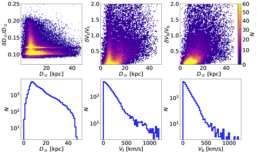
Figure 1: Distances and transverse velocities for stars in the Gclean catalogue (see Section 2.2). Top panels show density distributions in the plane of relative error (absolute value) and heliocentric distance. Bottom panels give distributions of the heliocentric distance and the components of the apparent (sky-projected) tangential velocity. Note that this plot also shows stars with $D_{\odot}>40\ \,{\rm kpc}$ that are eliminated in the final Gclean catalogue.

In the last two decades, wide-area multi-epoch surveys have brought in a rich harvest of variable stars in general and RRL in particular (e.g. Sesar et al., 2007; Soszyński et al., 2009; Drake et al., 2013; Soszyński et al., 2014; Torrealba et al., 2015; Sesar et al., 2017). Typically old and metal-poor, RRL have long served as a tried and true tracer of the Galactic halo and its sub-structures (e.g. Vivas et al., 2001; Morrison et al., 2009; Watkins et al., 2009; Sesar et al., 2013; Simion et al., 2014; Mateu et al., 2018; Hernitschek et al., 2018). Gaia, the first truly all-sky variability census in the optical, has further improved our understanding of the Milky Way RRL, not only by filling in the gaps left behind by the previous generations of surveys, but also by providing high-quality proper motions for the bulk of the RRL it sees. The Gaia data has thus enabled a new, precise characterisation of the Galactic halo density field (e.g. Iorio et al., 2018; Wegg et al., 2019; Iorio & Belokurov, 2019) and helped to discover halo sub-structures previously not seen (Belokurov et al., 2017; Koposov et al., 2019; Belokurov et al., 2019; Torrealba et al., 2019).

While it is true that RRL are being used primarily to trace the fossil record of the Milky Way assembly, it was always known that in the field, a relatively small number of metal-rich examples exist (Kukarkin, 1949; Preston, 1959; Smith, 1984; Layden, 1994; Walker & Terndrup, 1991; Dékány et al., 2018; Chadid et al., 2017; Fabrizio et al., 2019; Zinn et al., 2020). Based on their kinematics, these metal-rich RRL were assigned to the Galactic disc(s) (Layden, 1995a). Given the enormous number of available red giant progenitors, metal-rich RRL in the disc were estimated to form between 200 and 800 times less often compared to their old and metal-poor halo counterparts (Taam et al., 1976; Layden, 1995b). While the formation channel has not yet been identified, these early studies as well as the subsequent follow-up conjectured that the progenitors of metal-rich RRL ought to be old, i.e. $>10$ Gyr (e.g. Mateu & Vivas, 2018). The presence of likely old metal-rich RRL has been confirmed also in metal-rich Globular Clusters (e.g. NGC 6338 and NGC 6441, see Pritzl et al. 2000), however they have periods that are significantly larger with respect to field metal-rich RRL. The main obstacle to the production of a metal-rich RRL is its temperature on the HB: with higher envelope opacities, these stars tend to sit too far to the red from the instability strip (e.g. Dorman, 1992). Therefore, before arriving onto the HB, metal-rich RRL progenitors are required to undergo copious levels of mass-loss, $\approx 0.5$ M_⊙ or more, which may well be beyond what is physically possible.

Most recently, the conundrum of metal-rich RRL has been given a new lease of life. Marsakov et al. (2018) demonstrated that while plenty of the local metal-rich RRL likely belong to the thick disc (and thus can be as old as $\approx$10 Gyr), a substantial fraction displays the kinematics of the younger portion of the thin disc. An age of only few Gyrs would be very difficult to reconcile with the conventional scenarios of the RRL formation. Note that if extreme mass loss can be invoked, i.e. in excess of $1$ M_⊙, then even young ($>1$ Gyr) progenitors can produce metal-rich RRL (see Bono et al., 1997a, b). In a follow-up study, Marsakov et al. (2019) estimated the masses of the metal-rich thin disc RRL and found them to be of order of $0.5-0.6$ M_⊙, thus confirming the need for mass loss beyond the typically accepted values. Finally, Zinn et al. (2020) and Prudil et al. (2020) combined RRL with available spectroscopy with the Gaia DR2 astrometry to confirm the existence of metal-rich RRL stars with the orbital properties typical of the Galactic thin disc. With these most recent observations in hand, it remains to be seen if metal-rich RRL can actually be easily accommodated within the current stellar evolution theory. Comparing the structural properties of the metal-rich and metal-poor RRL, Chadid et al. (2017) conclude that it can not.

What is hard to achieve via single stellar evolution channels can (sometimes) be effortlessly done with binary stars. Indeed, an object has been discovered that nimbly mimics the classic RR Lyrae behaviour, i.e. lives on the instability strip and pulsates with the same kind of lightcurve, yet it is not an RR Lyrae, at least not in the conventional meaning of the term (Pietrzyński et al., 2012). This star, designated Binary Evolution Pulsator (BEP), is a low-mass ($0.26\ M_{\odot}$) remnant of mass transfer in a binary system with a period of $\approx 15$ days. As the follow-up theoretical work demonstrates, binary evolution can lead to a broad range of BEP masses, and in some cases even involve a stripped star with a helium-burning core (Karczmarek et al., 2017). These impostors would be indistinguishable from the classic RR Lyrae but have an age of only 4-5 Gyr. Only one such object has been found so far, but searches for RR Lyrae in binary systems are ongoing (e.g. Prudil et al., 2019b; Kervella et al., 2019).

This work aims to exploit the unprecedented all-sky coverage of Gaia to study the chemo-kinematics of the halo and the disc of the Milky Way as traced by RRL stars. The paper is organised as follows. Section 2 presents the construction of a clean sample of Gaia RRL stars and gives the details of the methods we use to estimate physical quantities like distance, metallicity and transverse velocity. Section 3 describes the machinery employed to perform the kinematic decomposition of the Galactic components. Then, we discuss the properties of the individual components: the halo in Section 4 and the disc in Section 5. In Section 6 we discuss possible biases affecting the results and finally, we summarise the main conclusions.

2 The sample

We use the whole catalogue of stars classified as RRL in Gaia DR2 (Gaia Collaboration et al., 2018a) combining the SOS (Specific Object Study, Clementini et al. 2019) RRL catalogue with the stars classified as RRL in the general variability table vari_classifier_result (Holl et al., 2018) following the procedure described in Iorio & Belokurov (2019). The initial combined catalogue contains 228,853 stars ($\approx 77\%$ RRab, $\approx 21\%$ RRc and $\approx 2\%$ RRd).

2.1 Distance and velocities estimate

One of the key ingredients of this analysis is the distance from the Sun, $D_{\odot}$, of each star. Once the heliocentric distance is known, we estimate the Galactocentric coordinates and, using the observed proper motion, calculate the velocities $V_{\ell}$ (along the Galactic longitude $\ell$) and $V_{b}$ (along the Galactic latitude).

Galactic parameters. We set a left-handed Galactocentric frame of reference similar to the one defined in Iorio et al. (2018): here $x$,$y$,$z$ indicate the Cartesian coordinates; $R$ is the cylindrical radius, $r$ is the spherical radius and $\phi$, $\theta$ represent the azimuthal and zenithal angle. In this coordinate system the Sun is located at $x_{\odot}=R_{\odot}=8.13\pm 0.3$ kpc (Gravity Collaboration et al., 2018) and $z_{\odot}=0$ kpc (see Iorio et al. 2018). In order to correct the observed stellar velocity for Sun’s motion, we adopt $V_{\mathrm{lsr}}=238\pm 9\ \,{\rm km\,s}^{-1}$ (Schönrich, 2012) for the local standard of rest (lsr) and $(U_{\odot},V_{\odot},W_{\odot})=(-11.10\pm 1.23,12.24\pm 2.05,7.25\pm 0.63)\ \,{\rm km\,s}^{-1}$ (Schönrich et al., 2010) for the Sun’s proper motion with respect to the lsr (assuming the Galactocentric frame of reference defined above). The final correcting vector is

$$V_{\mathrm{\odot,corr}}=(-11.10\pm 1.23,250.24\pm 9.23,7.25\pm 0.63).$$ (1)

In order to take into account all of the uncertainties in the estimate of the physical parameters of interest, we use a Monte-Carlo sampling method ($10^{5}$ realisations) following the steps: i) correction of Gaia $G$ magnitudes for the dust reddening, $ii)$ estimate of the metallicity, $iii)$ estimate of the absolute magnitude $M_{\mathrm{G}}$, $iv)$ estimate of the distance and the Galactocentric coordinates, $v)$, estimate of the velocities. Where not specified we sample the value of a given parameter $X=\bar{X}\pm\delta X$ drawing variates from a normal distribution centred on $\bar{X}$ and with a standard deviation $\delta X$.

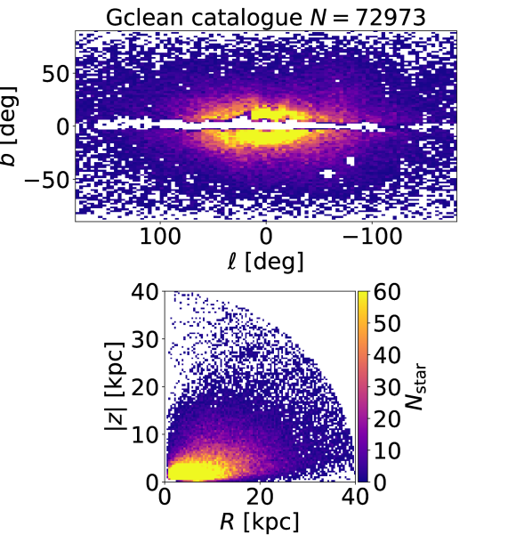
Figure 2: Galactic (top panel) and Galactocentric cylindrical (bottom panel) star count maps for objects in the Gclean catalogue (see Section 2.2)

Magnitude correction for dust reddening. We correct the observed $G_{\mathrm{obs}}$ magnitude as

$$G=G_{\mathrm{obs}}-k_{\mathrm{G}}E(B-V),$$ (2)

where $E(B-V)$ and its error, $\delta_{\mathrm{E(B-V)}}=0.16\times E(B-V)$, comes from Schlegel et al. (1998). The factor $k_{\mathrm{G}}$ is obtained by applying Equation 1 of Gaia Collaboration et al. (2018b) iteratively if the star has an estimate of the Gaia color $BP-RP$, otherwise we assume $k_{\mathrm{G}}=2.27\pm 0.30$ (Iorio & Belokurov, 2019). For the stars in the SOS catalogue, the adopted $G_{\mathrm{obs}}$ is the SOS table entry int_average_g and the color $BP-RP$ is the difference between the columns int_average_bp and int_average_rp. For the other stars, we use the values reported in the general Gaia source catalogue (phot_g_mean_mag, phot_bp_mean_mag, phot_rp_mean_mag). We notice a small offset ($\approx 0.03$ for $G_{\mathrm{obs}}$ and $\approx 0.02$ for $BP-RP$) between the SOS and general Gaia values, hence we correct the latter. We use the values from the SOS catalogue as standard for two reasons: they are estimated directly from the lightcurves (robust against outliers, see Clementini et al. 2019) and the magnitude-metallicity relation we use (see below) has been calibrated on these $G$ values (see Muraveva et al. 2018). After the offset correction, the differences between the SOS and Gaia observed magnitudes can be treated as another source of random errors on the estimate of $G$. For most of the stars in the sample (> 98 %) the magnitude of this error is $\lesssim 0.1\%$, representing a negligible amount in the error budget of the final distance estimate (see below). We decided to not consider the errors on $G_{\mathrm{obs}}$, thus the error on $G$ comes only from the uncertainties on $k_{\mathrm{G}}$ or $E(B-V)$.

Metallicity estimate. It is well known that the metallicities of RRL correlate with their lightcurve properties (e.g. Jurcsik & Kovacs 1996; Smolec 2005; Nemec et al. 2013; Hajdu et al. 2018). Two of the most used properties are the period (fundamental period, $P$ for RRab stars, first overtone period, $P_{\mathrm{1o}}$, for RRc stars) and the phase difference between the third and the first harmonics $\Phi_{31}$ of the lightcurve decomposition. Although the SOS catalogue already reports an estimate of the metallicity based on the Nemec et al. 2013 relations (see Clementini et al. 2019), we decide to use instead a linear relation calibrated directly on the Gaia $P$ (or $P_{\mathrm{1o}}$) and $\Phi_{31}$ parameters (see e.g. Jurcsik & Kovacs 1996). For the RRab stars we cross-match the SOS catalogue with the spectroscopic sample of Layden (1994) finding 84 stars in common and deriving the following relation:

$$\mathrm{[Fe/H]}_{\mathrm{RRab}}= (-1.68\pm 0.05)+(-5.08\pm 0.5)\times(P-0.6)$$ (3)

$$+(0.68\pm 0.11)\times(\Phi_{31}-2.0),$$

with an intrinsic scatter $\delta_{\mathrm{[Fe/H]}}=0.31\pm 0.03$. Concerning the RRc, following Nemec et al. (2013), we use the RRc stars in known Globular Clusters as classified by Gaia Collaboration et al. (2018d), then we assign to each of them the metallicity reported for the Globular Clusters in Harris (1996). Using this method we obtain the following metallicity relation:

$$\mathrm{[Fe/H]_{\mathrm{RRc}}}= (-1.26\pm 0.03)+(-9.39\pm 0.66)\times(P_{\mathrm{1o}}-0.3)$$ (4)

$$+(0.29\pm 0.05)\times(\Phi_{31}-3.5),$$

with an intrinsic scatter $\delta_{\mathrm{[Fe/H]}}=0.16\pm 0.03$. We sample the metallicity distribution for each star drawing from both the $P$ (or $P_{\mathrm{1o}}$) and $\Phi_{31}$ distributions considering their errors and from the posterior of the model parameters (taking into account their correlation). In case the star has not a period estimate and/or $\Phi_{31}$, these values are drawn from their overall 2D distribution considering the whole Gaia SOS catalogue. After this step we end up with $10^{5}$ [Fe/H] realisations for each star. Further information on the metallicity estimate can be found in the Appendix A.

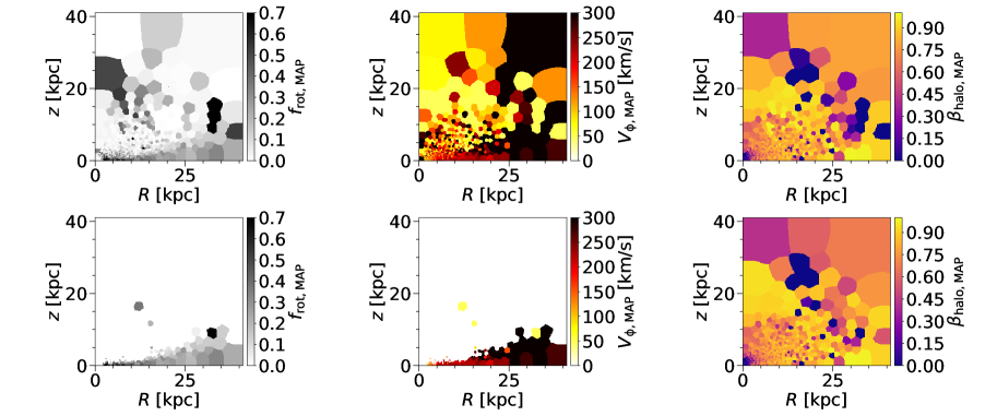
Figure 3: Top: results of the double-component fit for the RRLs in the Gclean sample (see Table 1). Maximum-a-posteriori (MAP) values are shown in cylindrical coordinates. Bottom: mixed 1 and 2 component results (results from the double-component fit if $\Delta\mathrm{BIC}>10$, otherwise from the single-component fit, see text for details). Left column shows the fraction of the rotating component, middle panels give the azimuthal velocity of the rotating component, while right column presents the anisotropy of the halo-like component.

Absolute magnitude. The absolute magnitudes are estimated using the $M_{\text{G}}-\mathrm{[Fe/H]}$ relation described in Muraveva et al. (2018). We sample the absolute magnitude distribution for each star using the $\mathrm{[Fe/H]}$ realisations (see above) and drawing the $M_{\text{G}}-\mathrm{[Fe/H]}$ relation parameters (taking into account the intrinsic scatter) using the errors reported by Muraveva et al. (2018).

Distance estimate. We produce $10^{5}$ realisations of the heliocentric distance using the familiar equation

$$\log\left(\frac{D_{\odot}}{\text{kpc}}\right)=\frac{G-M_{\mathrm{G}}}{5}-2.$$ (5)

Then, the heliocentric distance and the observed Galactic coordinates ($\ell$, $b$, taken without their associated uncertainties) are used to obtain realisations of the Galactocentric Cartesian, cylindrical and spherical coordinates ($x$,$y$,$z$,$R$,$r$,$\phi$,$\theta$) taking into account the errors on the Galactic parameters. Finally, we use the mean and the standard deviation of the final realisations to obtain the fiducial value and errors on the Galactic coordinates for each star.

Velocity estimate. We estimate the physical velocities from the observed proper motions as

$$V_{\ell} =K\mu_{\ell}D_{\odot}+V_{\ell,\odot}$$ (6)

$$V_{\mathrm{b}} =K\mu_{b}D_{\odot}+V_{\mathrm{b,\odot}}$$

where $K\approx 4.74$ is the conversion factor from $\text{mas}\ \text{kpc}\ \text{yr}^{-1}$ to $\text{km}\ \text{s}^{-1}$. $V_{\ell,\odot}$ and $V_{\mathrm{b,\odot}}$ represent the projection of the Sun velocity (Equation 1) in the tangential plane at the position of the star. These two values are estimated by applying the projection matrix defined in Equation A2 in Iorio et al. (2019) to the correcting vector in Equation 1. We draw $10^{5}$ realisations for each star taking into account the $D_{\odot}$ samples, the errors and the covariances of the proper motions and the errors on $V_{\mathrm{\odot,corr}}$. Then, we estimate the mean value, the standard deviation and the covariance between $V_{\ell}$ and $V_{\mathrm{b}}$. We use these values to perform our kinematic analysis (see Section  3).

2.2 Cleaning

In order to study the global properties of the (large-scale) Galactic components, we clean the RRL sample by removing the stars belonging to the most obvious compact structures (Globular Clusters and dwarf galaxies including the Magellanic Clouds) as well as various artefacts and contaminants. This procedure is similar to the cleaning process described in Iorio & Belokurov (2019), especially with regards to the cull of known Galactic sub-structures. Concerning the artefacts and contaminants, we employ a slightly different scheme in order to both maintain as many stars at low latitudes as possible and have more robust quality cuts. In particular, we focus on removing stars that could have biased astrometric solutions or unreliable photometry.

Artefacts and contaminants. Holl et al. (2018), Clementini et al. (2019) and Rimoldini et al. (2019) found that in certain regions (the bulge and the area close to the Galactic plane) the presence of artefacts and spurious contaminants in the Gaia’s RRL catalogues can be quite significant. The contaminants in these crowded fields are predominantly eclipsing binaries and blended sources, with a minute number of spurious defections due to misclassified variable stars (Holl et al., 2018). To remove the majority of the likely contaminants we apply the following selection cuts:

• $RUWE$<1.2

• $1.0+0.015\times(BP-RP)^{2}<BRE<1.3+0.06\times(BP-RP)^{2}$

• $E(B-V)$<0.8

The renormalised_unit_weight_error ($RUWE$) is expected to be around one for sources whose astrometric measurements are well-represented by the single-star five-parameter model as described in Lindegren et al. (2018). Therefore the above $RUWE$ cut eliminates unresolved stellar binaries (see e.g.  Belokurov et al., 2020b) as well as blends and galaxies (see e.g.  Koposov et al., 2017). The phot_bp_rp_excess_factor, $BRE$, represents the ratio between the combined flux in the Gaia $BP$ and $RP$ bands and the flux in the $G$ band, and thus by design is large for blended sources (see Evans et al., 2018). Following Lindegren et al. (2018), we remove stars with $BRE$ larger or lower than limits that are functions of the observed colors (Equation C2 in Lindegren et al. 2018). Finally, we remove stars in regions with high reddening, $E(B-V)$ (according to Schlegel et al., 1998), for which the dust extinction correction is likely unreliable. After these cuts, our RRL sample contains 115,774 RRL stars.

Globular clusters and dwarf satellites. We consider all globular clusters (GCs) from the Harris (1996) catalogue and all dwarf galaxies (dWs) from the catalogue published as part of the Python module galstream (Mateu et al. 2018). We select all stars within twice the truncation radius of a GC if this information is present, otherwise we use 10 times the half-light radius. For the dWs we take 15 times the half-light radius. Amongst the selected objects, we remove only the stars in the heliocentric distance range $D_{\mathrm{GC/dWs}}\pm 0.25\times D_{\mathrm{GC/dWs}}$. The chosen interval should be large enough to safely take into account the spread due to the uncertainty in the RRL distance estimate (see Section 2.1 and Figure 1). This procedure removes 1,350 stars.

Sagittarius dwarf. In order to exclude the core of the Sagittarius dwarf we select all stars with $|\tilde{B}-\tilde{B}_{\text{Sgr}}|<9^{\circ}$ and $|\tilde{\Lambda}-\tilde{\Lambda}_{\text{Sgr}}|<50^{\circ}$, where $\tilde{B}$ and $\tilde{\Lambda}$ are the latitude and longitude in the coordinate system aligned with the Sagittarius stream as defined in Belokurov et al. (2014) and $\tilde{B}_{\text{Sgr}}=4.24^{\circ}$ and $\tilde{\Lambda}_{\text{Sgr}}=-1.55^{\circ}$ represent the position of the Sagittarius dwarf. Then, among the selected objects, we get rid of all stars with a proper motion relative to Sagittarius lower than $2\ \text{mas}\ \text{yr}^{-1}$, considering the dwarf’s proper motion from Gaia Collaboration et al. (2018d). The stars in the tails have been removed considering all the objects within $|\tilde{B}-\tilde{B}_{\text{Sag}}|<11^{\circ}$ and with proper motions (in the system aligned with the Sgr stream) within 1.5 mas yr^-1 from the proper motions tracks of the Sgr stream (D. Erkal private communication, the tracks are consistent with the ones showed in Ramos et al. 2020). The cuts of the core and tails of the Sgr dwarf remove 7,233 stars.

Magellanic Clouds. We apply the same selection cuts as those used in Iorio & Belokurov (2019) thus removing 14,987 stars (11,934 for the LMC and 3,053 for the SMC).

Cross-match with other catalogues. In order to identify possible classification mistakes and other contaminants, we cross-match the catalogue scrubbed of substructures and artefacts (as described above) with the $SIMBAD$ astronomical database (Wenger et al., 2000), the $CSS$ periodic variable table (Drake et al., 2017) and the $ASAS$-$SN$ catalogue of variable stars (Jayasinghe et al., 2018, 2019a, 2019b). We remove all stars that have not been classified as: RRLyr, CandidateRRLyr, HB*, Star, Candidate_HB*, UNKNOWN, V*, V*? in $Simbad$ (1,015 stars); RRab, RRc or RRd in $CSS$ (655 stars) or $ASAS$-$SN$ (11,963 stars). Analysing these data we found a low level of contamination (stars not classified as RRL in the cross-matched catalogue $\lesssim 3\%$) considering $Simbad$ and $CSS$, while the level of contamination considering $ASAS$-$SN$ is ten times larger ($\approx 27\%$). However, as most of the contaminants are classified as UNKNOWN ($\approx 20\%$) in $ASAS$-$SN$, these objects could suffer from poor lightcurve sampling. Another significant contaminant class is eclipsing binaries, mostly W Ursae Majoris variables (WUMa, $\approx 5\%$) for which the lightcurve could be misclassified as an RRc. Indeed, among the stars classified as WUma in $ASAS$-$SN$ about $80\%$ are classified as RRc in the Gaia SOS catalogue. Not considering the dominant sources of contamination discussed above, the number of unwanted interlopers estimated from $ASAS$-$SN$ is similar to that obtained with $Simbad$ and $CSS$. Comparing the RRL classification for the stars in common between the Gaia SOS catalogue and the Gaia general variability catalogue we decided to remove all stars that have been classified as RRd (2941 stars) in at least one of the two catalogues. In total these cuts remove 15,633 stars.

Distance cut. Given the significant increase in velocity uncertainties at large distance, we decide to limit the extent of our sample to within 40 kpc from the Galactic centre. This cut removes 4,057 stars.

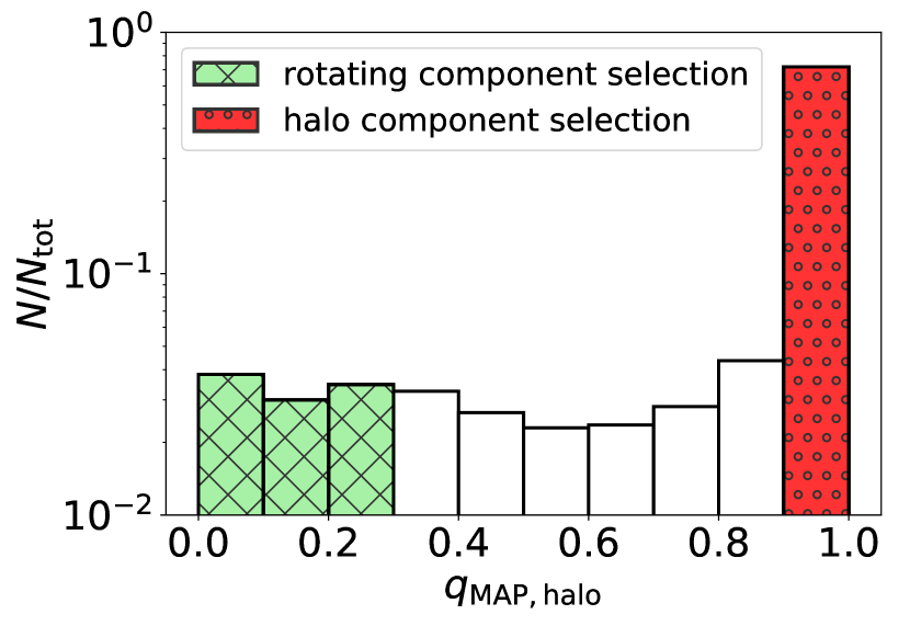
Figure 4: Distribution of the RRL maximum-a-posteriori probability (MAP, see Section  3.1) of belonging to the non-rotating (halo) kinematic component from the double component fit described in Section  3.3. The red o-hatched and the green x-hatched regions indicate the $q_{\mathrm{MAP,halo}}$ cuts used to select the halo and the rotating (disc-like) subsample respectively.

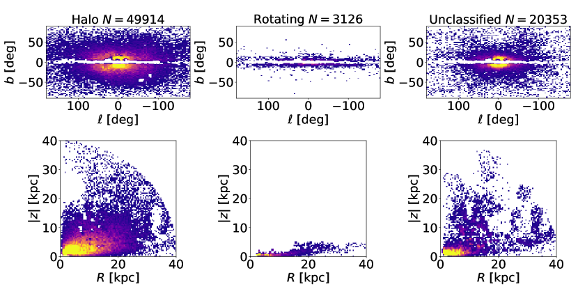
Figure 5: Three RRL groups. Same as Figure 2 but for the stars in the Gclean catalogue (Section 2.2) belonging to the halo sub-sample (left), rotating disc-like subsample (centre) and stars that satisfy neither of the above criteria (right), see Section 3.3 for details. The color-map is the same as that shown in Figure 2.

The final cleaned catalogue contains $72,973$ stars (Gclean catalogue). We also produce a very conservative catalogue considering only the stars that have been classified as RRab in both Gaia SOS and $ASAS$-$SN$ ($17,570$ stars, SA catalogue), we also require that they have complete Gaia lightcurve information (period and $\Phi_{31}$). In the rest of the paper, we will compare the results of the analysis of the two catalogues to investigate potential biases due to artefacts and contaminants that went unnoticed. The distributions of heliocentric distances and of the transverse velocities in the Gclean catalogue are shown in the bottom panel of Figure 1 (displaying the sample before the distance cut). Most of the stars are located within 20-25 kpc from the Sun, but there are still hundreds of stars out to approximately 40 kpc; beyond this radius, the number of objects in the catalogue decreases abruptly (these objects are not present in the final Gclean catalogue). The relative distance and velocities uncertainties are shown in the top panels of Figure 1: four sequences are clear in the left-hand panel. The vertical sequence located around 8-10 kpc is due to the stars in highly-extincted regions where the uncertainties on the reddening dominate the error budget (see Section 2.1). The higher horizontal sequence ($\delta D_{\odot}/D_{\odot}\approx 0.12$) comprises of the stars without the period estimate. The other two sequences are due to stars without $\Phi_{\mathrm{31}}$ estimate ($\delta D_{\odot}/D_{\odot}\approx 0.11$) and to stars in the SOS catalogue with complete information (period and $\Phi_{\mathrm{31}}$, $\delta D_{\odot}/D_{\odot}\approx 0.10$). Overall most of the stars have distance errors slightly larger than 10%, while the relative errors on velocities can reach substantial values (up to $50-100\%$). The errors reported in Figure 1 are random errors based on the Monte-Carlo analysis (Section 2.1), however we also analyse the possible systematic effects due to the assumptions made when information about the period and/or when $\Phi_{31}$ and/or the Gaia colors is not available (Section 2.1). For most of the cases, the systematic shift is sub-dominant (relative error$\approx 5\%$) with respect to the random errors. Hence, we do not include a systematic component in the uncertainties used in the kinematic analysis. Based on the error properties of the catalogue we expect that our analysis (Section 3) is able to give reliable constraints on the kinematic parameters within 20-30 kpc from the Galactic centre, while the quality of the results progressively degrades at large radii. The distribution of the stars on the sky and in the Galactocentric $R,|z|$ plane are shown in the left-hand column of Figure 2.

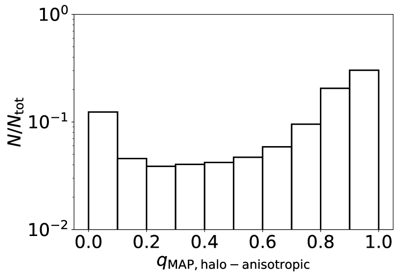
Figure 6: Distribution of the RRL maximum-a-posteriori probability (MAP, see Section 3.1) of belonging to the (radially) anisotropic kinematic component as inferred from the double component fit described in Section 3.3.

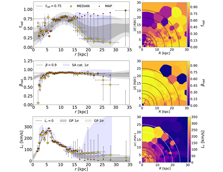
Figure 7: Properties of the radially-anisotropic halo component (see Section 4.1): relative fraction of the radial component over the total (top), its anisotropy (middle) and the position of the peak of the double-horn profile assumed for the distribution of the radial velocity (bottom, see Section 4). Left (right) panels show the results of the model applied to spherical (cylindrical) Voronoi bins (see Section 3.2 and Section 4). The large yellow data-points give the median of the a-posteriori distribution, while the error-bars indicate its 16th and 84th percentile; the small-red points show the Maximum-a-Posteriori (MAP) of the posteriors; X-axis represents the median of the spherical radial distribution, while the errorbars indicate the median value of the errors on the radius of the stars in each bin; the grey bands show the $1\sigma$ and $2\sigma$ interval from a Gaussian Process (GP) interpolation. We interpolate the symmetrised version of the data points with a GP process: data-points show the middle values between the 16th and 84th percentile, while the vertical error-bars are half of the 16th-84th percentile distance; the blue band shows the 1$\sigma$ interval of the posterior obtained using the SA (SOS+$ASAS$-$SN$) catalogue (see Section  2.2). The circular lines indicate the spherical radii of 5,8,10,15,20,25 kpc.

3 The Method

This work aims to study the kinematics of the RRL stars in the Gaia dataset. Such an analysis is however hampered by the lack of line-of-sight (los) velocity measurements for most of the stars in our final catalogue – indeed only 266 out of more than $70,000$ stars have Gaia radial velocity. Relying on cross-matches with other spectroscopic catalogue such as $RAVE$ (Kunder et al., 2017), $APOGEE$ (Majewski et al., 2017), or $LAMOST$ (Cui et al., 2012) would reduce the number of objects as well as the radial extent and sky coverage of the catalogue. Moreover, the periodic radial expansion/contraction of the RRL surface layers, if not taken into account, can bias the radial velocity measurements by up to $40-70\ \,{\rm km\,s}^{-1}$ (see e.g. Liu, 1991; Drake et al., 2013).

The lack of the los velocities makes it impossible to estimate the full 3D velocity information on a star-by-star basis. However, since stars at different celestial coordinates and different heliocentric distances have distinct projections onto the 3D Galactic velocity space, it is possible to estimate the velocity moments (mean values and standard deviations) of the intrinsic 3D velocity ellipsoid using the proper motions of a group of stars taken together under the assumptions of symmetry (see e.g. Dehnen & Binney, 1998; Schönrich et al., 2012; Schönrich & Dehnen, 2018; Wegg et al., 2019). In practice, we consider two possibilities and assume that proper motions of stars i) at the same $R$ and $|z|$ (cylindrical symmetry) or ii) the same $r$ (spherical symmetry) sample the same 3D velocity distribution.

3.1 Kinematic fit

In what follows we implement the ensemble velocity moment model following and extending the method described in Wegg et al. (2019) (W19, hereafter). In this section we briefly summarise the method; further details can be found in the original W19 paper. The basic assumption is that the intrinsic velocity distribution of stars in a given Galactic volume at given Galactocentric coordinates (e.g. spherical or cylindrical) is a multivariate normal $f\left(\bm{V}\right)=\mathcal{N}\left(\bar{\bm{V}},\Sigma\right)$, where $\bar{\bm{V}}$ is the Gaussian centroid and $\Sigma$ is the covariance matrix or velocity dispersion tensor. This distribution can be projected onto the heliocentric sky coordinates $\bm{V}_{\mathrm{sky}}=(V_{\mathrm{los}},V_{\ell},V_{b})$ appliyng the rotation matrix $\mathbf{R}$ (different for each sky position) satisfying $\bm{V}_{\mathrm{sky}}=\mathbf{R}\bm{V}$. The projected distribution is still a Gaussian and therefore it can be easily analytically marginalised over the unknown term $V_{\mathrm{los}}$. Finally, the likelihood for a given star located at given distance and position on the sky to have velocities $\bm{V}_{\mathrm{\perp}}=(V_{\ell},V_{b})$ is given by

$$\mathcal{L}=\mathcal{N}\left(\bar{\bm{V}}_{\mathrm{\perp}},\Lambda_{\perp}+\mathbf{S}\right),$$ (7)

where

• $\bar{\bm{V}}_{\mathrm{\perp}}=\mathbf{R}_{\perp}\bar{\bm{V}}$ and $\mathbf{R}_{\perp}$ is the rotation matrix $\mathbf{R}$ without the 1st row related to the los velocity ($2\times 3$ matrix, see Appendix B);

• $\Lambda_{\perp}$ is the projected covariance matrix $\Lambda=\mathbf{R}\mathbf{\Sigma}\mathbf{R}^{\intercal}$ without the 1st row and the 1st column related to the los velocity ($2\times 2$ matrix);

• $\mathbf{S}$ is a 2x2 matrix of the $V_{\ell},V_{b}$ measurement errors and covariance (see Section  2.1).

In order to estimate the velocity moments, we consider the total likelihood as the product of the likelihoods (Equation 7) of all stars in a given Galactic volume bin. The method described so far follows, point by point, what has been done in W19. We add a further generalisation considering the intrinsic velocity distribution as a composition of multiple multivariate normal distributions. Therefore the likelihood for a single star becomes

$$\mathcal{L}_{\mathrm{multi}}=\sum_{i}f_{i}\mathcal{N}\left(\bar{\bm{V}}_{i,\mathrm{\perp}},\Lambda_{i,\perp}+\mathbf{S}_{i}\right)=\sum_{i}f_{i}\mathcal{L}_{i},$$ (8)

where the component weights $f$ sum up to 1. Using Equation 8 we can apply a Gaussian Mixture Model to the intrinsic velocity distribution fitting only the observed tangential velocities. Starting form Equation 8 it is possible to define, for each star, the a-posterior likelihood of belonging to the $i$th component as

$$q_{i}=\frac{f_{i}\mathcal{L}_{i}}{\mathcal{L}_{\mathrm{multi}}}.$$ (9)

The stochastic variables $q$ (and their uncertainties) allow us to decompose the stars into different kinematic populations using a quantitative “metric". For a given sample of stars (see Section  3.2), we retrieve the properties ($\bm{V},\mathbf{\Sigma}$) (3+6 parameters) of the kinematic components and their weights adopting a Monte Carlo Markov Chain (MCMC) to sample the posterior distributions generated by the product of all likelihoods defined in Equation 8. In practice, the posterior distributions have been sampled using the affine-invariant ensemble sampler MCMC method implemented in the Python module emcee (Foreman-Mackey et al., 2013). We used 50 walkers evolved for 50000 steps after 5000 burn-in steps. We evaluate the convergence of the chains by analysing the trace plots and estimating the autocorrelation time $\tau_{f}$ (see e.g. Goodman & Weare 2010). In particular, we check that for all of our fits and parameters, the number of steps is larger than $50\tau_{f}$, i.e. the number is sufficient to significantly reduce the sampling variance of the MCMC run. All kinematics models have been run and analysed using the Python module Poe.

In the next Sections, we exploit this method to separate the RRL sample into two distinct kinematic components: a non-rotating (or weakly rotating) halo-like population and a population with a large azimuthal velocity. Subsequently, the same method is applied again to separate kinematically the halo into an anisotropic and an isotropic populations. The choice of binning in the given coordinate system (spherical or cylindrical), the number of Gaussian components and the prior distributions of their parameters are described in the following Sections.

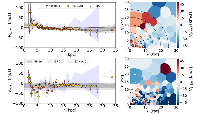
Figure 8: Same as Figure 7 but for the azimuthal velocity for the radially-anisotropic (left-hand panel) and the isotropic (right-hand panel) components.

3.2 Binning strategy

Each of our kinematic analyses is applied to stars grouped in bins of Galactic $r$ or $R,|z|$ assuming spherical or cylindrical symmetry correspondingly. In each of these bins the intrinsic distribution of velocities is considered constant. In order to have approximately the same Poisson signal-to-noise ratio ($\sqrt{N_{\mathrm{stars}}}$) in each bin we compute a Voronoi tessellation of the $R,|z|$ plane making use of the vorbin Python package (Cappellari & Copin, 2003). When assigning stars to bins in spherical $r$, we select the bin edges so that each bin contains $N_{\mathrm{stars}}$ objects. If the outermost bin remains with a number of stars lower than $N_{\mathrm{stars}}$, we merge it with the adjacent bin. In the rest of the paper, we identify the coordinates of a given bin ($R,|z|$ or $r$) as the median of the coordinate of the stars in the bin, we associate to these values an error that is the median of the corresponding errors of the stars. Although we do not take account explicitly of the errors on $R$,$|z|$ and $r$ in the kinematic fit, the velocities $V_{\ell}$ and $V_{b}$ already incorporate the errors on distance (Section 2.1). In practice, we do not allow stars to belong to more than one bin even if this is consistent with their Galactic coordinate errors. This choice does not represent a serious issue in our analysis, but at large radii, where the errors are larger, the kinematic parameters obtained with our fit are likely correlated in adjacent bins.

3.3 Kinematic separation

	Prior distributions
	halo	rotating
$V_{\mathrm{\phi}}$	$\delta(0)$	$\mathcal{N}(100,200)[50,\infty]$
$V_{\mathrm{r}}=V_{\mathrm{\theta}}$	$\delta(0)$
$\sigma_{\mathrm{r}}$	$\mathcal{N}(150,200)[0,\infty]$	$\mathcal{N}(0,20)[0,\infty]$
$\sigma_{\mathrm{t}}$	$\mathcal{N}(100,200)[0,\infty]$
$\rho_{\mathrm{r}\phi}=\rho_{\mathrm{r}\theta}=\rho_{\phi\theta}$	$\delta(0)$
$f$	$\mathcal{U}(0,1)$

Table 1: Prior distributions for the parameters of the double-component fit: non-rotating halo/rotating components (Section 3.3). Both components are multivariate normals defined in a Galactocentric spherical frame of reference (see Section 2.1). The parameters are from the top to the bottom: centroids of the normal distribution, velocity dispersions (assuming $\sigma_{\mathrm{t}}=\sigma_{\mathrm{\phi}}=\sigma_{\mathrm{\theta}}$ and $\sigma_{\mathrm{r}}=\sigma_{\mathrm{t}}$ for the isotropic component), covariance terms of the velocity dispersion tensor, weight of one of the component (see Equation 8). The used distributions are: Dirac Delta, $\delta$; normal, $\mathcal{N}(\bar{x},\sigma_{\mathrm{x}})$ where $\bar{x}$ is the centroid and $\sigma_{\mathrm{x}}$ the standard deviation; uniform, $\mathcal{U}(x_{\mathrm{low}},x_{\mathrm{up}})$ where $x_{\mathrm{low}}$ and $x_{\mathrm{up}}$ represent the distribution limits. The squared bracket indicate the distribution boundary, i.e. the prior probability is 0 outside the given range. If the brackets are not present the boundary is set to $[-\infty,\infty]$. All the velocity centroids and velocity dispersions are in unit of $\,{\rm km\,s}^{-1}$. Considering the parameters drawn from Dirac Delta as fixed in the fit, the total number of free parameters is 5.

In order to separate the non-rotating halo from a component with a high azimuthal velocity we set up a double-component fit:

• 1st component (halo-like): spherical frame-of-reference, no rotation ($V_{\mathrm{\phi}}=0$), anisotropic velocity dispersion tensor (we fit the the radial, $\sigma_{\mathrm{r}}$, and tangential, $\sigma_{\mathrm{t}}=\sigma_{\mathrm{\phi}}=\sigma_{\mathrm{\theta}}$, velocity dispersion.).

• 2nd component (rotating): spherical frame of reference, isotropic velocity dispersion tensor.

In both cases the centroids along $V_{\mathrm{r}}$ and $V_{\mathrm{\theta}}$ are set to 0. We assume that the velocity ellipsoids are aligned in spherical coordinates fixing to 0 the diagonal terms of the velocity dispersion tensor (see e.g. Evans et al., 2018). Table 1 summarises the model parameters and their prior distributions. In particular, we set non-exchangeable priors for the velocity centroids and velocity dispersions to break labelling degeneracy (switching between models in the MCMC chains) and improve model identifiability. In order to detect possible overfitting due to the double-component assumption, we also run a single-component fit considering only the halo model summarised in Table 1. The significance of the more complex double component fit is analysed with the Bayesian Information Criterion (BIC) using the maximum-a-posteriori (MAP) of the likelihood, $\mathcal{L}_{\mathrm{MAP}}$:

$$\mathrm{BIC}=k\ln n-2\ln\mathcal{L}_{\mathrm{MAP}},$$ (10)

where $k$ is the number of free parameters and $n$ is the data sample size. The model with the lowest BIC is preferred, in particular we consider significant the results of the two component fit where the BIC difference ($\Delta\mathrm{BIC}$) is larger than 10. In order to apply the fit we separate the whole sample (72,973 stars) into 692 cylindrical $R,|z|$ bins with an average Poisson signal-to-noise ratio of 10 (see Section 3.2). The fit is applied separately in each bin.

Figure 3 presents the maps of the kinematic properties of the two principal components, the halo and the disc in cylindrical $R$ and $|z|$. The two rows give the same information, but the bottom row shows the results of the double-component fit only if there is a significant improvement as indicated by the Bayesian Information Criterion $\Delta{\rm BIC}>10$, otherwise it reverts to the results of a single-component fit. The first column shows the map of the fractional contribution of the rotating component. While there are some hints of rotating parts of the halo at high $|z|$ in the top panel, as demonstrated by the bottom panel, these are not significant enough. The bulk of the rotating component sits at $|z|<5$ kpc across a wide range of $R$, and closer to the Sun its vertical extent is clearly limited to a couple of kpc at most. The second column presents the map of the azimuthal velocity $V_{\phi}$ as a function of $R$ and $|z|$. Again, some Voronoi cells at high $|z|$ may have the kinematics consistent with a slow rotation, however $\Delta{\rm BIC}$ criterion renders them not significant enough. Therefore, in the bottom row, these high $|z|$ cells are empty and the bulk of the $V_{\phi}$ map is limited to low vertical heights where the rotation velocity is in excess of $V_{\phi}>200$ kms^-1 across the entire range of $R$. Two single bins at high $z$ with $R\approx 10-15\ \,{\rm kpc}$ survive the BIC cut, they show an azimuthal rotation of $\approx 50\ \,{\rm km\,s}^{-1}$. Stars in these bins are likely related to the rotating halo structure found in the unclassified sample and discussed in Section 6.1. Finally, the third column displays the behaviour of the halo velocity anisotropy $\beta$ as mapped by RRL. Except for a small region near the centre of the Milky Way and a few cells at high $|z|$ where the motion appears nearly isotropic, the rest of the halo exhibits strong radial anisotropy with $0.6<\beta<0.9$.

Figure 4 shows the distribution of the posterior probability of belonging to the non-rotating (halo) component for the stars in our sample. Going from $q_{\mathrm{MAP,halo}}=1$ to $q_{\mathrm{MAP,halo}}=0$, the distribution can be divided in three regions: a clear peak around $q_{\mathrm{MAP,halo}}=1$, these are the RRL that do not exhibit any significant rotation and thus can be confidently assigned to the halo; a decreasing trend in the number fraction ranging from $q_{\mathrm{MAP,halo}}\approx 0.9$ to $q_{\mathrm{MAP,halo}}\approx 0.5$; finally, a region with an increasing number fraction from $q_{\mathrm{MAP,halo}}\approx 0.5$ to $q_{\mathrm{MAP,halo}}=0$. The latter region is likely populated by the stars with disc-like kinematics (closer to 0 is $q_{\mathrm{MAP,halo}}$, more robust is the association with the rotating component), while the second region is composed of stars that do not fall squarely into one of the two groups. Setting this latter, undetermined group aside for now, we focus on the stars that can be classified as halo or disc with certainty. We select the halo and disc-like stars by applying the following cuts:

$$\begin{split}\mathrm{halo}&:q_{\mathrm{MAP,halo}}>0.9\ \&\ q_{\mathrm{16th,halo}}>0.5\\ \mathrm{rotatingdisc-like}&:q_{\mathrm{MAP,halo}}<0.3\ \&\ q_{\mathrm{84th,halo}}<0.5\\ \ \ &\&\ \ |z|<5\ \,{\rm kpc}\ \&\ \Delta\mathrm{BIC}>10,\end{split}$$ (11)

where $q_{\mathrm{16th,halo}}$ and $q_{\mathrm{84th,halo}}$ are the 16th and 84th percentile of the a-posteriori $q_{\mathrm{halo}}$ distribution. The selection cut for the halo is straightforward (see Fig. 4), the additional cut on the 16th percentile has been added to conservatively remove stars with poorly constrained $q_{\mathrm{halo}}$. The $q_{\mathrm{MAP,halo}}$ cut for the disc-like component is somehow arbitrary but we find it the best compromise between a large enough number of stars (to have good statistics) and to be conservative enough to target the stars that are more “purely" associated with the rotating component. The other conditions has been added to focus on the disc-like flattened structure ($z$ cut) and to remove portion of the Galaxy volume where the presence of two-component is not statistically significant (BIC cut).

Of the total 72,973 RRL in our sample, 49,914 (or $\approx 68\%$) are classified as halo, 3,126 (or $\approx 4\%$) as disc; while the remaining 19,993 ($\approx 28\%$) are unclassified. Figure 5 shows the distribution of the three kinematic groups on the sky in Galactic coordinates (top row) and in cylindrical $R,|z|$ (bottom row). The halo stars (first column) span a wide range of Galactic latitudes but mostly reside in a centrally concentrated, slightly flattened structure limited by $R<30$ kpc and $|z|<20$ kpc. The middle panels of Figure 5 clearly show that the rotating component has a disc-like spatial distribution and extends to R $\approx$ 30 kpc (see also the bottom panels of Figure 3). Interestingly, a similarly-extended and highly flattened distribution was already detected previously in the sample of candidate-RRL stars selected in the first Gaia data release (Iorio et al., 2018).

Finally, the shape of the unclassified portion of our sample (third column) resembles a superposition of the disc and the halo, albeit more concentrated to the centre: most of the stars are at $R<10$ kpc and $|z|<5$ kpc. Additionally, at higher $|z|$, there are several lumps and lobes likely corresponding to parts of the Virgo Overdensity and the Hercules Aquila Cloud (e.g. Vivas et al., 2001; Vivas & Zinn, 2006; Belokurov et al., 2007; Jurić et al., 2008; Simion et al., 2014; Simion et al., 2019).

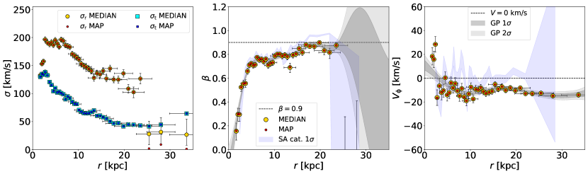
Figure 9: Same as Figure 7 but for the anisotropy (middle panel) and the azimuthal velocity (right-hand panel) estimated in the single-component fit of the halo catalogue (see Section  4). The left-hand panel shows the radial and tangential velocity dispersion.

Our kinematic decomposition unambiguously demonstrates the presence of a disc-like population amongst the Gaia RRL. According to the left panel of Figure 3, this rapidly rotating population contributes from $\approx 30\%$ (outer disc) to up to $\approx 50-60\%$ (inner disc) of the RRL with $|z|<1$ kpc. We also see clear signs of the RRL disc flaring beyond 15 kpc (see first two panels in the bottom row of the Figure). This is unsurprising as the restoring force weakens with distance from the Galactic centre (see e.g. Bacchini et al., 2019). Additionally, the Milky Way disc at these distances is withstanding periodic bombardment by the Sgr dwarf (e.g. Laporte et al., 2018, 2019). The structure of the outer disc as traced by RRL is consistent with the recent measurements of the Galactic disc flare (e.g. López-Corredoira & Molgó, 2014; Dékány et al., 2019; Thomas et al., 2019; Skowron et al., 2019). In what follows, we consider the halo and the disc RRL sub-samples, selected using criteria listed in Equation 11, separately.

4 The halo RR Lyrae

	Prior distributions
	halo-anisotropic	halo-isotropic
$V_{\mathrm{\phi}}$	$\mathcal{N}(0,100)$	$\mathcal{N}(0,100)$
$V_{\mathrm{r}}=V_{\mathrm{\theta}}$	$\delta(0)$
$L_{\mathrm{r}}\dagger$	$\mathcal{N}(0,300)[0,\infty]$	$\delta(0)$
$\sigma_{\mathrm{r}}$	$\mathcal{N}(150,100)[0,\infty]$	$\mathcal{N}(100,20)[0,\infty]$
$\sigma_{\mathrm{t}}$	$\mathcal{N}(50,50)[0,\infty]$
$\rho_{\mathrm{r}\phi}=\rho_{\mathrm{r}\theta}=\rho_{\phi\theta}$	$\delta(0)$
$f$	$\mathcal{U}(0,1)$

Table 2: Same as Table 1 but for the double component fit: halo-anisotropic/halo-isotropic components. $\dagger$The halo-anisotropic component is a superposition of two multivariate normals (with same normalisation) offset from each other in $V_{\mathrm{r}}$ space by $2L_{\mathrm{r}}$ (see Section 4). The total number of free parameters is 7.

As convincingly demonstrated by Lancaster et al. (2019), the kinematic properties of the Galactic stellar halo can not be adequately described with a single Gaussian. This is because the inner $\approx 30$ kpc are inundated with the debris from the Gaia Sausage event (see e.g. Belokurov et al., 2018b; Myeong et al., 2018b), also known as Gaia Enceladus (see e.g. Helmi et al. 2018; Koppelman et al. 2020 but see also Evans 2020), producing a striking bimodal signature in the radial velocity space. Lancaster et al. (2019) devise a flexible kinematic model to faithfully reproduce the behaviour of an ensemble of stars on nearly radial orbits (see also Necib et al., 2019, for a similar idea). We use the halo model developed by Lancaster et al. (2019) and Necib et al. (2019) to describe the kinematics of the halo sub-sample (see Section 3.3). More precisely, the model is the mixture of two components: isotropic and anisotropic, both of which can rotate, i.e. have non-zero mean $V_{\mathrm{\phi}}$. The model, its parameters and their prior distributions are summarised in Table 2. The prior distributions of the anisotropic component reflect our knowledge of the radially-anisotropic nature of the halo. Moreover, they are set up to help the convergence of the chain and the model identifiability as discussed in Section 3.3. By testing on the mock dataset we ensure that the chosen priors are not preventing the selection of isotropic ($\sigma_{\mathrm{r}}=\sigma_{\mathrm{t}}$) or tangentially-anisotropic models ($\sigma_{\mathrm{r}}<\sigma_{\mathrm{t}}$) or models with simple Gaussian distribution along $V_{\mathrm{r}}$ ($L_{\mathrm{r}}\approx 0$). This two-component model with 7 free parameters is applied to the halo sub-sample (49,914 stars) twice: once in bins of $r$ and again in bins of $R$ and $|z|$ (see Section 3.2). In the first case we use 41 bins with an average Poisson signal-to-ratio of 35, in the second case the bins are 203 with an average signal-to-ratio of 15. Parameters of both components are allowed to vary from bin to bin. For comparison, we also model the RRL kinematics in the halo sub-sample with a single anisotropic multivariate normal with 4 free parameters: $V_{\mathrm{\phi}}$ (prior $\mathcal{N}(0,100)$), $\sigma_{\mathrm{r}}$, $\sigma_{\mathrm{\phi}}$, $\sigma_{\mathrm{\theta}}$ (prior $\mathcal{N}(0,200)[0,\infty]$).

Note that in our analysis, we do not attempt to distinguish between the bulge and the halo RR Lyrae. This is because many of the classical bulge formation channels are not very different from those of the stellar halo, especially when both accreted and in-situ halo components are considered (see e.g. Kormendy & Kennicutt, 2004; Athanassoula, 2005). Historically, quite often the term “bulge" is used to refer simply to the innermost region of the Milky Way. In that case, the Galactic bar and the discs would be included (see e.g. Barbuy et al., 2018). However, we do not believe that these additional in-situ populations contribute significantly to the dataset we are working with. This is because our sample is highly depleted in the inner, low $|z|$ portion of the Galaxy where the RR Lyrae distribution is at its densest and the most complex, i.e. $R<2$ kpc. For example, we do not have any stars with $R<1$ kpc; there are only $\sim$2700 ($\sim$200) stars in the main (SA) sample with $R<2$ kpc.

4.1 Kinematic trends in the halo

For stars in the halo sub-sample, Figure 6 shows the distribution of the posterior probability of membership in either of the two components. As evidenced in the Figure, the anisotropic component is dominant in this particular dataset. Figure 7 presents the properties of the anisotropic halo population. Given the high values of $\beta$ displayed in the middle row of the Figure, we identify this component with the Gaia Sausage debris (see Iorio & Belokurov, 2019, for discussion of the GS as traced by the RRL). It is important to note that, in some cases, the median and the maximum-a-posteriori (MAP) points in Figure 7 show large differences because the posterior distribution is bimodal. In those cases, the median results are closer to the minimum that has been sampled more, while the error-bars do not correspond to the classical Gaussian 1$\sigma$ errors but rather the distance between the two minima sampled by the MCMC. Despite the large uncertainties due to the bimodal distribution, the MAP and the median estimates indicate similar behaviour: if we consider the MAP, the fraction of the radial component remains high but $L_{\mathrm{r}}$ drops to 0; if we consider the median, $L_{\mathrm{r}}\approx 50\ \,{\rm km\,s}^{-1}$, but the fraction drops to small values. Therefore, both the MAP and median indicate a transition between the strong radially anisotropic component and the rest of the stellar halo.

The top row of Figure  7 gives the contribution of the stars in the radially-dominated portion of the halo as a function of $r$. This fraction is at its lowest ($\approx 20\%$) near the Galactic centre. Outside of $R=3$ kpc, stars on nearly-radial orbits contribute between $50\%$ and $80\%$. Beyond $R=20$ kpc, this fraction becomes highly uncertain. From the right panel in the top row, it appears that the contribution of the radially-biased debris falls slightly faster with $|z|$, as expected if the debris cloud is flattened vertically. The middle row of Figure 7 presents the behaviour of the velocity anisotropy $\beta$ with Galactocentric radius $R$ (left) and $R$ and $|z|$ (right). Note that in the model with two $V_{\mathrm{r}}$ humps, anisotropy $\beta$ can increase i) when radial velocity dispersion dominates or ii) when the velocity separation between the two humps $2L_{r}$ increases. For stars in the radial component, $\beta$ is relatively low at $\beta\approx 0.3$ in the inner 3 kpc, but grows quickly to $\beta=0.9$ at 5 kpc and stays flat out to 20 kpc. Finally, the bottom panel of the Figure shows the radial velocity separation $L_{r}$. It reaches maximum $L_{r}\approx 270$ kms^-1 around $3<R<5$ kpc from the Galactic centre and then drops to $L_{r}\approx 0$ kms^-1 around 30 kpc. The trend of $L_{r}$ as a function of $R$ looks very similar to the projection of a high-eccentricity orbit onto the phase-space $(V_{r},R$). Along such an orbit, the highest radial velocity is reached just before the pericentre crossing, where it quickly drops to zero. The orbital radial velocity decreases more slowly towards the apocentre where it also reaches zero. As judged by the bottom row of Figure 7, the pericentre of the GS progenitor (in its final stages of disruption) ought to be around $2<R<3$ kpc, while its apocentre somewhere between $R=20$ kpc and $R=30$ kpc.

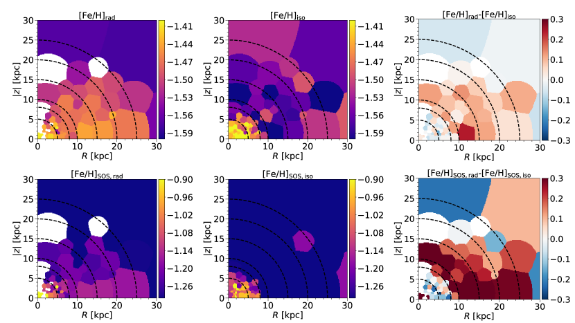
Figure 10: Cylindrical maps showing the distributions of the median metallicity estimated in this work (top, see Section  2.1 and Appendix A) and reported in the SOS catalogue (bottom) respectively. Left-hand panels show the metallicity maps for the stars in the radially-biased halo component (23,734 stars) while the middle panels show the stars in the isotropic halo component (7,767 stars). The right-hand panels show the difference between the radial and the isotropic component maps. The stars in this map are subsamples of the halo component (see Section  4) belonging to the SOS catalogue and with an a-posteriori MAP likelihood of belonging to the anisotropic or isotropic component larger than 0.7 (see Figure 6). The Voronoi-tesselation has been obtained using the isotropic halo sample with a target Poisson signal-to-noise equals to 10. The bins in which the number of stars is lower than 50 are excluded from the maps (see e.g. the white bins in the left-hand and right-hand panels).

In Figure 7 as well as in several subsequent Figures we compare the kinematic properties of the Gaia DR2 RRL sample (Gclean) with those obtained for a more restrictive set of RRL, i.e. that produced by cross-matching the objects reported in the Gaia SOS and by the $ASAS$-$SN$ variability survey (SA catalogue, shown as light lilac filled contour). The SA catalogue does not only suffer lower rate of contamination, it contains only bona fide RRab stars with period information and, therefore, much more robust (and unbiased) distance estimates. This more trustworthy RRL dataset comes at a price: the size of the SA sample is $\approx 5$ times smaller compared to the Gclean catalogue and the sampled distances are reduced by the magnitude limit ($V\approx 17$) of the $ASAS$-$SN$ dataset. Reassuringly, however, the differences between the kinematic properties of the radially-biased halo component inferred with the Gclean and the SA data are minimal as demonstrated in the left column of Figure 7. The only clear distinction worth mentioning is the blow-up of the $L_{r}$ confidence interval shown in the bottom left panel. Beyond 15 kpc, the SA-based $L_{r}$ uncertainty explodes due to the lack of distant RR Lyrae in this sample.

Figure 8 is concerned with the mean azimuthal velocity of each of the two halo components. Mean $V_{\mathrm{\phi}}$ is shown for the radial (top) and the isotropic (bottom) portions of the model applied to the halo sample. For the GS-dominated radially-biased halo component, $V_{\mathrm{\phi}}$ is slightly prograde ($\approx 15$ kms^-1) within the Solar circle and becomes slightly retrograde ($\approx-15$ kms^-1) outside of 10 kpc. Note that net rotation is particularly affected by hidden distance biases (as discussed in e.g. Schönrich et al., 2011) and is driven by over- or under- correcting for the Solar reflex motion (see Section 6.2). The mean azimuthal velocity of the radially-biased component of the halo plays an important role in reconstructing the details of the GS merger. As discussed in Belokurov et al. (2018b), the Sausage progenitor galaxy did not necessarily have to arrive to the Milky Way head-on. Instead, the dwarf could start the approach with plenty of angular momentum which it then lost as it coalesced and disrupted in the Galaxy’s potential. The idea that dynamical friction could cause the orbit of a massive satellite to radialise instead of circularising was first proposed in Amorisco (2017). A clearer picture of the azimuthal velocity behavior is given by the SA dataset, which is much less susceptible to distance errors, and as a consequence to $V_{\phi}$ biases. The SA probability contours show that the net rotation of the radially-biased halo component remains very slightly prograde (at the level of $\approx 15$ kms^-1) throughout the Galactocentric distance range probed. Such slight prograde spin is in agreement with a number of recent studies (see Deason et al., 2017; Tian et al., 2019; Wegg et al., 2019; Belokurov et al., 2020a). Note that this low-amplitude prograde rotation can only be claimed with some degree of confidence at distances $R<10$ kpc, i.e. the region containing a larger portion of RRL in our sample. Further out in the halo, the net azimuthal velocity is consistent with zero (see also Bird et al., 2020; Naidu et al., 2020). For the isotropic halo component, both Gclean and SA datasets indicate a slight retrograde net rotation ($\approx-20$ kms^-1), at least in the inner Galaxy.

Figure 9 offers a view of the Galactic stellar halo as described by a single Gaussian component. It is not surprising to see the behaviour which appears to be consistent with an average between the strongly radial and isotropic components shown in the previous Figures. Between 5 and 25 kpc, the velocity anisotropy is high $0.75<\beta<0.9$, only slightly lower than that shown in the top left panel of Figure 8. Similarly, the superposition of slightly prograde and slightly retrograde populations yields a mean azimuthal velocity consistent with zero (as previously reported e.g. by Smith et al., 2009) as measured for the SA sample (see filled pale lilac contours in the right panel of the Figure). The Gclean dataset gives a retrograde bias of $-10$ kms^-1. Remember however that a portion of the halo was excised and is now a part of the ‘unclassified’ subset. These ‘unclassified’ RRL ought to be considered to give the final answer as to the net rotation of the halo (see Section 6.1).

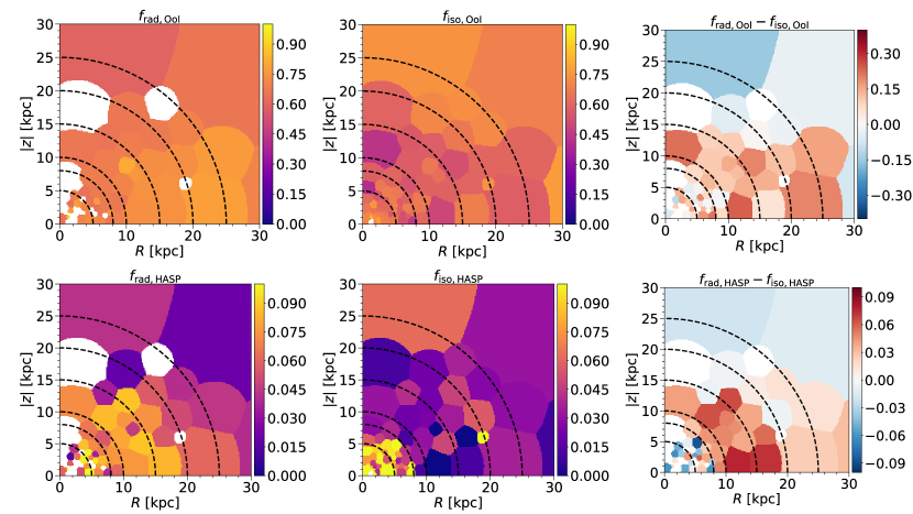
Figure 11: Same as Figure 10 but for the Oosterhoff Type 1 (OoI, top panels) and the High Amplitude Short Period (HASP, bottom panels) fractions. See Section 4.2 and Belokurov et al. (2018a).

4.2 Stellar population trends in the halo

Belokurov et al. (2018b) used $SDSS$+Gaia DR1 data to establish a tight link between the velocity anisotropy and the metallicity in the local stellar halo. They show that the highest values of $\beta\approx 0.9$ are achieved by stars with metallicity $-1.7<$[Fe/H]$<-1.2$, while at lower metallicities the anisotropy drops to $0.2<\beta<0.4$. Using a suite of zoom-in simulations of the MW halo formation, the prevalence in the Solar neighborhood of comparatively metal-rich halo stars on highly eccentric orbits is interpreted by Belokurov et al. (2018b) as evidence for an ancient head-on collision with a relatively massive dwarf galaxy. In this picture, the lower-anisotropy and lower-metallicity halo component is contributed via the accretion of multiple smaller Galactic sub-systems. Note that strong trends between orbital and chemical properties in the Galactic stellar halo had been detected well before the arrival of the Gaia data (see e.g. Eggen et al., 1962; Chiba & Beers, 2000; Ivezić et al., 2008; Bond et al., 2010; Carollo et al., 2010). Most recently such chemo-kinematic correlations have been observed in glorious detail in multiple studies that used the GDR2 astrometry (e.g. Myeong et al., 2018a; Deason et al., 2018; Lancaster et al., 2019; Conroy et al., 2019; Das et al., 2020; Bird et al., 2020; Feuillet et al., 2020). Consequently, in the last couple of years, a consensus has emerged, based on the numerical simulations of stellar halo formation and chemical evolution models, that the bulk of the local stellar halo debris is contributed by a single, old and massive (and therefore relatively metal-rich) merger (see Haywood et al., 2018; Helmi et al., 2018; Mackereth et al., 2019a; Fattahi et al., 2019; Bignone et al., 2019; Bonaca et al., 2020; Renaud et al., 2020; Elias et al., 2020; Grand et al., 2020).

Figure 10 explores the connection between the RR Lyrae kinematics and their metallicity (estimated from the lightcurve shape, see Section  2.1 and Appendix A). Both the top and the bottom row use the sample of halo stars contained in the SOS catalogue of Gaia DR2 RRL. In the top row, we present the metallicity maps obtained using our [Fe/H] calibration presented in Equations  3 and  4. The bottom row uses the metallicity estimates reported as part of the SOS catalogue. While the two rows display different absolute mean values of [Fe/H] in the halo (due to different calibrations used), the relative metallicity changes as a function of $R$ and $|z|$ and between the two halo components look very similar. The left column of Figure 10 shows the metallicity distribution in the radially-biased halo component. As discussed above, the bulk of this halo population has likely been contributed by the Gaia Sausage merger. Both top and bottom panels reveal a slightly flattened ellipsoidal structure whose metallicity is elevated compared to the rest of the halo. This [Fe/H] pattern extends out to $R\approx 30$ kpc and $|z|\approx 20$ kpc. No significant metallicity gradient is observed in the radial direction, although the inner 2-3 kpc do appear to be more metal-rich. However, given the behaviour of $L_{r}$ shown in Figure 7, we conjecture that very little Gaia Sausage debris reaches the inner core of the Galaxy (see Section 4.1 for discussion). In the vertical direction, there are hints of a metallicity gradient where [Fe/H] decreases with increasing $|z|$.

The behaviour of [Fe/H] in the isotropic halo component is given in the middle column of Figure 10. The most striking feature in the metallicity distribution of the isotropic component is the compact spheroidal structure with $R<10$ kpc whose mean metallicity exceeds that of the radially-anisotropic component (and hence that of the Gaia Sausage). Beyond $R\approx 10$ kpc, no strong large-scale metallicity gradient is discernible: [Fe/H] does change appreciably and stays at levels slightly lower than those achieved by the GS debris at similar spatial coordinates. To contrast the metallicity trends of the two halo components, the right column of the Figure shows the difference of the left and middle metallicity distributions. This differential picture highlights dramatically the shape of the GS debris cloud whose mean metallicity sits some $0.2$ dex above the typical halo [Fe/H] value. Even more metal-rich is the inner 10 kpc. This inner halo structure - which also appears flattened in the vertical direction - exhibits the highest mean metallicity in the inner 30 kpc of the halo, at least $0.2$ dex higher than the radially-biased GS.

The position of an RRL on the period-amplitude plane contains non-trivial information about its birth environment. In the Milky Way halo, globular clusters show a well-defined ‘Oosterhoff dichotomy’ (Oosterhoff, 1939, 1944) where RRL in clusters of Oosterhoff Type I (OoI) have a shorter mean period compared to those in GCs of Oosterhoff Type II (OoII). The ‘Oosterhoff dichotomy’ is not present in the dwarf spheroidals observed today around the Milky Way that appear to contain mixtures of Oosterhoff types but not in arbitrary proportions (e.g. Catelan, 2004, 2009). Thus, the relative fraction of RRL of each Oosterhoff type can be used to decipher the contribution of disrupted satellite systems to the Galactic stellar halo (see e.g. Miceli et al., 2008; Zinn et al., 2014). Finally, the so-called High Amplitude Short Period (HASP) RRL can be found across the Milky Way but are rather rare amongst its satellites. This allowed Stetson et al. (2014) and Fiorentino et al. (2015) to put constraints on the contribution of dwarf galaxies of different masses to the Galactic stellar halo. Most recently, Belokurov et al. (2018a) used RRL tagging according to their type (OoI, OoII or HASP) to ‘unmix’ the Milky Way halo. Taking advantage of the wide-area RRL catalogue provided as part of the Catalina Real-Time Transient Survey (Drake et al., 2013, 2014; Drake et al., 2017), they show that the fraction of OoI RRL changes coherently and dramatically as a function of Galactocentric distance. They also demonstrate that in the Milky Way dwarf spheroidal satellites, the OoI fraction increases with dwarf’s mass. Using a suite of Cosmological zoom-in simulations, Belokurov et al. (2018a) conjecture that the radial evolution in the RR Lyrae mixture is driven by a change in the fractional contribution of satellites of different masses. More precisely, they interpret the peak in the OoI fraction within $R\approx 30$ kpc as evidence that the Milky Way’s inner halo is dominated by the debris of a single massive galaxy accreted some 8-11 Gyr ago. This picture is confirmed by the change in the HASP RRL at $10<R$(kpc)$<30$. However, inwards of $R\approx 10$ kpc, the HASP fraction grows further, to levels significantly higher than those displayed in the most massive MW satellites such as LMC, SMC and Sgr, making the very core of the halo unlike any satellite on orbit around the Galaxy today. Note that the Oosterhoff and HASP classes are used here simply as a way to select particular regions on the period-amplitude plane. The exact position on this so called Bailey diagram has remained a useful RR Lyrae diagnostic tool for decades but is only now starting to be investigated thoroughly with the help of the Gaia data and high-resolution spectroscopy (see e.g. Fabrizio et al., 2019).

Figure 11 follows the ideas discussed in Belokurov et al. (2018a) and tracks the fraction of OoI type (top) and HASP (bottom) RRL as a function of $R$ and $|z|$ in both radially-biased (left) and isotropic (middle) halo components. Additionally, the difference between the two maps is shown in the right column of the Figure. As the Figure demonstrates, the OoI and HASP fractions in the radially-biased halo component are higher compared to the isotropic halo population. In comparison, the RRL in the inner $\approx 10$ kpc show slightly lower OoI contribution, yet the HASP fraction is higher. These trends in the period-amplitude of halo RRL are fully consistent with those presented in Belokurov et al. (2018a) and support the picture in which the RRL on highly eccentric orbits originate from a single massive and relatively metal-rich dwarf galaxy. Given its lower metallicity, lower fraction of OoI and HASP RRL, the isotropic population could be a superposition of tidal debris from multiple smaller sub-systems.

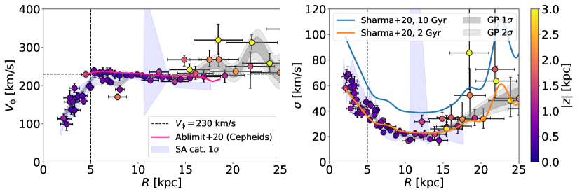
Figure 12: Azimuthal velocity and velocity dispersion (assuming isotropy) obtained for the sample of rotating stars (see Section 5). Y-axis gives the median of the a-posteriori distribution of the azimuthal velocity, while the errorbars indicate its 16th and 84th percentile. X-axis shows the median of the cylindrical radial distribution, while the error-bars indicate the median value of the errors on the cylindrical radius of the stars in the given bin. Vertical black dashed lines mark 5 kpc radius roughly corresponding to the region where the presence of the bar may be important. The horizontal dashed line in the left panel indicates $V_{\mathrm{\phi}}=230\ \,{\rm km\,s}^{-1}$. Grey bands show the $1\sigma$ and $2\sigma$ intervals from the Gaussian Process interpolation as described in Figure 7. Blue band shows the 1$\sigma$ interval of the posterior obtained using the SA (SOS+$ASSASN$) catalogue (see text). The blue SA band explodes around $R\approx 12$ kpc due to a particular bin where most of stars have been classified as the background. The magenta line in the left-hand panel shows the azimuthal velocity measured by Ablimit et al. (2020) using a sample of Cepheids. The blue and orange lines in the right-hand panel show the median of the combination of the vertical and radial velocity dispersion model predictions by Sharma et al. (2020). Here we assumed [Fe/H]=$-1.0$ (see Figure 14), $z=0.5\ \,{\rm kpc}$ and stellar age $t=2\ \,{\rm Gyr}$ (orange line) and $t=10\ \,{\rm Gyr}$ (blue line), see text in Section 5 for further information.

As Figures 7, 10 and 11 reveal, the inner $5$-$10$ kpc of the Galactic stellar halo look starkly distinct from both the metal-richer radially-biased Gaia Sausage debris cloud and the metal-poorer isotropic halo. Belokurov et al. (2018a) suggested that a third kind of accretion event is required to explain the RRL properties in the inner Milky Way. This hypothesis, however, must be revisited in light of the Gaia data. Thanks to the Gaia DR1 and DR2 astrometry, we now have a better understanding of the composition of the Galactic stellar halo within the Solar radius. In particular, there now exist several lines of evidence that perhaps as much as $\approx 50\%$ of the nearby halo could be formed in situ. The earliest evidence for such a dichotomy in the stellar halo could be found in Nissen & Schuster (2010) who identified two distinct halo sequences in the $\alpha$-[Fe/H] abundance plane. Using Gaia DR1 astrometry complemented with $APOGEE$ and $RAVE$ spectroscopy, Bonaca et al. (2017) showed that approximately half of the stars on halo-like orbits passing through the Solar neighborhood are more metal-rich than [Fe/H]$=-1$ and were likely born in-situ. Gaia Collaboration et al. (2018b) used Gaia DR2 data to build a colour-magnitude diagram of nearby stars with high tangential velocities and showed that the Main Sequence of the kinematically-selected halo population is strongly bimodal. Subsequently, Haywood et al. (2018), Di Matteo et al. (2019) and Gallart et al. (2019) used Gaia DR2 to investigate the behaviour of the stars residing in the blue and red halo sequences uncovered by Gaia Collaboration et al. (2018b). All three studies agreed that the blue sequence is provided by the accreted tidal debris while the stars in the red sequence were likely formed in-situ. Both Di Matteo et al. (2019) and Gallart et al. (2019) point out that the stars in the in-situ component had likely formed before the accretion of Gaia Sausage and were heated up onto halo orbits as a result of the merger. It remains somewhat unclear however where the thick disc stops and the in-situ halo starts.

Belokurov et al. (2020a) used the catalogue of stellar orbital properties and accurate ages produced by Sanders & Das (2018) to isolate the halo component they dubbed the ‘Splash’. Splash contains stars with high metallicities $-0.7<[Fe/H]<-0.2$ and low-angular momentum (or retrograde) motion. Importantly, its azimuthal velocity distribution does not appear to be an extension of the thick disc’s – it stands out as a distinct kinematic component (see also Amarante et al., 2020). The age distribution of the Splash population shows a sharp drop around 9.5 Gyr in agreement with previous estimates described above. Belokurov et al. (2020a) used Auriga (Grand et al., 2017) and Latte (Wetzel et al., 2016) numerical simulations of Milky Way-like galaxy formation to gain further insight into the Splash formation. They demonstrate that a Splash-like population is ubiquitous in both simulation suites and indeed corresponds to the ancient Milky Way disc stars ‘splashed’ up onto the halo-like orbits (as conjectured by e.g. Bonaca et al., 2017; Di Matteo et al., 2019; Gallart et al., 2019). Most recently, Grand et al. (2020) provided a detailed study of the effects of the Gaia Sausage-like accretion events on the nascent Milky Way. They show that the propensity to Splash formation can be used to place constraints on the properties of the Gaia Sausage accretion event, for example the mass ratio of the satellite and the host. Additionally, they demonstrate that in many instances in their suite, the accretion is gas-rich and leads to a star-burst event in the central Milky Way. Interestingly, as pointed out by Belokurov et al. (2020a), recent observations of intermediate-redshift galaxies reveal that star-formation can originate in the gas outflows associated with profuse AGN or star-formation activity (see Maiolino et al., 2017; Gallagher et al., 2019; Veilleux et al., 2020) thus raising a question of whether the Milky Way’s Splash could also originate in the gas outflow (see also Yu et al., 2020).

While the earlier studies of the Galactic in-situ halo had been limited to the Solar neighborhood (Nissen & Schuster, 2010; Bonaca et al., 2017; Haywood et al., 2018; Di Matteo et al., 2019; Gallart et al., 2019), Belokurov et al. (2020a) provide the first analysis of the overall spatial extent of this structure. Using a selection of spectroscopic datasets, they show that the Splash does not extend much beyond $R\approx 15$ kpc and $|z|\approx 10$ kpc. Compare the picture in which the Splash looks like a miniature halo - or perhaps a blown-up bulge - (see red contours in Figures 11 and 13 in Belokurov et al. 2020a) and the RRL stellar population maps presented here in Figures 10 and  11. There is a very clear correspondence between the metal-rich and HASP-enhanced portion of the (mostly) isotropic halo population and the Splash. We therefore conjecture that the inner $\approx$10 kpc of the Galactic halo RRL distribution is pervaded by the in-situ halo population. The in-situ halo RRL are metal-rich and have lower mean OoI fraction compared to Gaia Sausage and possess the highest mean HASP fraction amongst all halo components.

5 The disc RR Lyrae

	Prior distributions
	disc	background
$V_{\mathrm{\phi}}$	$\mathcal{N}(0,400)[0,\infty]$
$V_{\mathrm{R}}=V_{\mathrm{z}}$	$\delta(0)$
$\sigma=\sigma_{\mathrm{R}}=\sigma_{\mathrm{z}}=\sigma_{\mathrm{\phi}}$	$\mathcal{N}(0,200)[0,\infty]$
$\rho_{\mathrm{R}\mathrm{z}}=\rho_{\mathrm{R}\phi}=\rho_{\mathrm{z}\phi}$	$\delta(0)$
$\bar{V_{\ell}}$		$\delta(\langle V_{\ell,\mathrm{stars}}\rangle)$
$\bar{V_{b}}$		$\delta(\langle V_{b,\mathrm{stars}}\rangle)$
$\sigma_{\ell}$		$\mathcal{C}(0,500)[0,\infty]$
$\sigma_{b}$		$\mathcal{C}(0,500)[0,\infty]$
$\rho_{\ell,b}$		$\mathcal{U}(-1,1)$
$f$	$\mathcal{U}(0,1)$

Table 3: Same as Table 1 but for the parameters of the double component fit: rotating-disc/background. The rotating-disc component is a 3D multivariate normal distribution defined in a Galactocentric cylindrical frame of reference (see Section  2.1) with parameters: centroids ($V_{\mathrm{\phi}}$,$V_{\mathrm{R}}$,$V_{\mathrm{z}}$), isotropic velocity dispersion $\sigma$ and correlation terms of the velocity dispersion tensor $\rho$. The background is modelled as 2D multivariate normal in the observed velocity space. The parameters are the centroids ($\bar{V_{\ell}},\bar{V_{b}}$), which are fixed to the average values of the observed velocity distribution of the stars in each bin, the velocity dispersions ($\sigma_{\ell},\sigma_{b}$) and the velocity correlation ($\rho_{\ell,b}$). $\mathcal{C}(x_{\mathrm{c}},l)$ indicates the Chaucy distribution centred in $x_{\mathrm{c}}$ and with scale $l$. The total number of free parameters is 6.

As described in Section 3.3, a small but significant fraction of the GDR2 RRL (just under $5\%$) are classified as belonging to a rotating component based on their kinematics. Figures 3 and 5 demonstrate that the stars in the rotating sample are heavily biased towards low Galactic latitude $|b|$ and small height $|z|$ and thus likely represent a Milky Way disc population. Here we provide a detailed discussion of the properties of this intriguing specimen.

In order to take into account possibile residual contaminants and outliers in the sample of rotating RRL (see Section  3.3) we set a double component fit (see e.g. Hogg et al. 2010):

• 1st component (disc-like): cylindrical frame-of-reference, isotropic velocity dispersion tensor, azimuthal velocity as the only streaming motion ($V_{\mathrm{R}}=V_{\mathrm{z}}=0$);

• 2nd component (background): observed velocity space ($V_{\ell}$,$V_{b}$), the centroid is fixed to the median of the observed velocity distribution, the velocity dispersion and the velocity covariance are free parameters.

Table 3 summarises the model parameters and their prior distributions, the number of free parameters is 6.

We apply the fit to the subsample of 3,126 rotating RRL (see Section 3.3 and Equation 11) grouped in 60 cylindrical Voronoi-cells (see Section 3.2) with an average Poisson signal-to-noise of $\approx 7$. For each region in the $R,|z|$ plane our kinematic model provides an estimate of the rotational velocity as well as the properties of the velocity ellipsoid and an estimate of the background level. After our analysis, we found a low level of contaminating background ($\approx 12\%$ of stars have $q_{\mathrm{bkg}}>0.7$) confirming that our subsample is a quite clean view of the rotating disc-like RRL population.

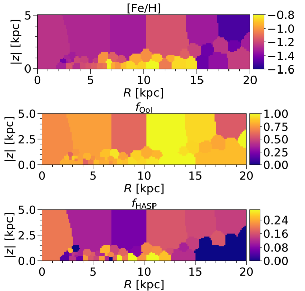
Figure 13: Stellar population properties of the rotating disc-like component in cylindrical coordinates. Top panel gives the median of the metallicity, middle panel shows the fraction of OoI type RR Lyrae, while the bottom panel presents the fraction of HASP stars. These maps use a subsample of the disc catalogue (see Section 5) obtained considering only objects belonging to the SOS catalogue (1841 stars). Each bin contains at least ten stars. The metallicities shown in this figure have been estimated through Equations 3 and 4 (see Appendix A).

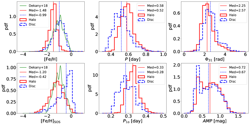
Figure 14: Lightcurve properties of a subsample of SOS stars in the Gclean catalogue (see Section  2.2) belonging to the halo (red, see Section  4) and the disc components (blue, see Section  5). From top-left to bottom-right the panels show the metallicity estimated in this work (see Section 2.1 and Appendix A), the period of the RRab stars, the lightcurve phase difference $\Phi_{\mathrm{31}}$ (see Section  2.1), the metallicity from Gaia SOS, the period of the RRc stars and the lightcurve amplitude in the Gaia $G$ band. The vertical dashed lines give medians of the distributions. Green curves in the left-hand panels show the best Gaussian Mixture Models of the photometric metallicity distribution of the sample of disc RRLs in Dékány et al. (2018). Only stars that have estimates of both the period and the lightcurve phase difference have been considered for this plot (24,598 and 1,146 stars from the halo and disc sample, respectively).

Figure 12 shows the mean azimuthal velocity (left) and velocity dispersion (right) as a function of the Galactocentric cylindrical radius $R$. The colour of the symbols represents their height above the plane $|z|$. The left panel of the Figure displays a well-behaved rotation curve traced by RRL: starting around $V_{\phi}\approx 100$ kms^-1 at distances of 2-3 kpc from the centre of the Galaxy, it quickly rises to $V_{\phi}\approx 230$ kms^-1 at $R\approx 5$ kpc, and then stays relatively flat at $5<R$(kpc)$<25$. Note that such high rotational velocities are characteristic of the thin disc population of the Milky Way. Overplotted on top of our measurements is the magenta line representing the azimuthal velocity curve of the thin disc Cepheids recently reported by Ablimit et al. (2020) and consistent with the kinematics of other thin disc tracers (e.g. Red Giants, Eilers et al. 2019; López-Corredoira & Molgó 2014). In the range of Galactocentric distances sampled by both the Cepheids and the RRL their azimuthal velocities are in complete agreement, thus vanquishing any remaining doubt about the nature of the fast-rotating RRL.

Stars in the Galactic disc are exposed to a variety of processes which can change their kinematics with time. Repeated interactions with non-axisymmetric structures such as the spiral arms, the bar and the Giant Molecular Clouds (with additional likely minor contribution from in-falling dark matter substructure) result in the increase of the stellar velocity dispersion, more pronounced for older stars, often described as Age Velocity dispersion Relation or AVR (see e.g. Strömberg, 1946; Spitzer & Schwarzschild, 1951; Barbanis & Woltjer, 1967; Wielen, 1977; Lacey, 1984; Sellwood & Carlberg, 1984; Carlberg & Sellwood, 1985; Carlberg, 1987; Velazquez & White, 1999; Hänninen & Flynn, 2002; Aumer & Binney, 2009; Martig et al., 2014; Grand et al., 2016; Moetazedian & Just, 2016; Aumer et al., 2016; Mackereth et al., 2019b; Ting & Rix, 2019; Frankel et al., 2020). Most recently, Sharma et al. (2020) used a compilation of spectroscopic datasets and Gaia DR2 astrometry to study the dependence of radial and vertical velocity dispersions for stars with $3<R$(kpc)$<20$. They use a combination of stellar tracers, Main Sequence Turn-Off stars and Red Giant Branch stars whose ages are calculated using spectro-photometric models calibrated with asteroseismology. Sharma et al. (2020) demonstrate that the stellar velocity dispersions are controlled by four independent variables: angular momentum, age, metallicity and vertical height. Moreover they show that the joint dependence of the dispersion on these variables is described by a separable functional form.

The right panel of Figure 12 compares the RRL velocity dispersions (under the assumption of isotropy) to the median between radial and vertical dispersion approximations obtained by Sharma et al. (2020). Here we have fixed other model parameters to the values most appropriate for our dataset, i.e. [Fe/H]=-1 and $|z|=0.5$. First thing to note is that the shape of the radial dispersion curve traced by the Gaia RRL matches remarkably well the behaviour reported by Sharma et al. (2020) for the disc dwarfs and giants. Secondly, the RRL velocity dispersion at the Solar radius is strikingly low, around $\approx 20$ kms^-1. Overall, both the shape and the normalisation of the RRL velocity dispersion agree well with that predicted for a stellar population of 2 Gyr in age (orange curve). In comparison, an older age of 10 Gyr would yield a dispersion almost twice as large (blue curve). Given the high azimuthal velocity and low velocity dispersion, as demonstrated in Figure 12 for both the Gclean and SA catalogues, we conclude that our sample of rotating RRL is dominated by a relatively young thin disc population. Note that as a check, we also perform a more detailed analysis obtaining an age estimate by fitting the velocity dispersions with the median (radial and vertical) model prediction from Sharma et al. (2020), considering all stars in the disc-like subsample and their properties and errors ([Fe/H], $R$, $z$, $V_{\phi}$ and $\sigma$ from the kinematic fit). This yields an age distribution consistent with a young disc population: the peak is at $\approx 2\,{\rm Gyr}$ and the wings extend from very young ages ($<1\ \,{\rm Gyr}$) to 5-7 Gyr.

Our findings are in agreement with those reported in the literature recently (e.g. Marsakov et al., 2018; Zinn et al., 2020; Prudil et al., 2020) that demonstrate the presence in the Solar neighborhood of RRL with thin disc kinematics and chemistry. For the first time, however, we are able to map out the kinematics of the disc RRL across a wide range of Galactocentric $R$ and show that their velocity dispersion behaviour is clearly inconsistent with that of an old population. Moreover, as demonstrated in the bottom row of Figure 3, beyond $R\approx 20\ \,{\rm kpc}$ we detect prominent flare in the spatial distribution of the disc RRL (compare to e.g. López-Corredoira & Molgó, 2014; Thomas et al., 2019). Note that the increase of the mean Galactic height with $R$ detected here is gentler compared to the above studies, thus also pointing at a younger age of these RRL in agreement with the maps presented in Cantat-Gaudin et al. (2020). Figure 13 zooms in on the rotating disc-like component and shows the properties of its stellar population (inferred from the RRL lightcurve shapes) as a function of cylindrical coordinates. From top to bottom, the panels show metallicity (top), OoI fraction (middle) and HASP fraction (bottom). Across the three panels, the disc RR Lyrae show consistent behaviour: their metallicity, OoI and HASP fractions remain high for $|z|<1$ kpc. For $3<R$(kpc)$<15$, radial behaviour shows no trends, but in the very inner Galaxy, metallicity and HASP fractions drop. Similarly, there appears to be a decrease in metallicity and HASP fraction in the outer parts of the disc, beyond $R=15$ kpc. The apparent central “hole” in the disc RRL population is consistent with the radial offset of the metal-rich component presented in Dékány et al. (2018) and in Prudil et al. (2020). The central depression can also be an indication of radial migration for the disc RRL population (see e.g. Beraldo e Silva et al. 2020). However, for our sample we can not rule out that some of the change in the inner 3 kpc at low $|z|$ is driven by the cleaning criteria applied (e.g. extinction cut) or increasing contamination from other components (bulge/bar, thick disc). The synchronous change in the RRL metallicity and the HASP fraction points to the fact that HASP objects are simply the high tail of the RR Lyrae [Fe/H] distribution.

Finally, let us contrast the lightcurve shapes of the halo and the disc RRL. Figure 14 presents the distributions of metallicity, period $P$, amplitude and phase difference $\phi_{31}$ for the halo (red) and the disc (blue) samples. We give two [Fe/H] distributions computed using two different calibrations: the top left panel of the Figure relies on the metallicity estimated using Equations 3 and 4, while the bottom left panel employs [Fe/H] values reported by Gaia’s SOS. Irrespective of the calibration used, the metallicities attained by the disc RRL are significantly higher than those in the halo. The [Fe/H] distribution of the rotating population exhibits a long tail towards low metallicities, but the peak (and the median) value is higher by 0.5 (0.8) dex depending on the calibration used. Given that the RRL metallicities are computed using only the period and phase difference, we expect that both $P$ and $\phi_{31}$ distributions should show clear differences when the halo and the disc RRL are compared. This is indeed the case as revealed by the middle column and the top right panel of Figure 14. The main difference is in the period distribution: the disc RRL have a shorter period on average. There is also a slight prevalence of lower values of $\phi_{31}$ while the amplitude distributions are not distinguishable. This behavior is in happy agreement with the properties of the disc RRL populations gleaned from smaller local samples (see e.g. Marsakov et al., 2018; Zinn et al., 2020; Prudil et al., 2020).

6 Discussion and Conclusions

6.1 The unclassified stars

So far, we have left out a substantial $\approx 25\%$ of the total RR Lyrae dataset as “unclassified”. Note that according to our definition, any sample of stars with intermediate properties, i.e. a population that does show either a strong prograde rotation (disc) or a zero mean azimuthal velocity (halo) would be deemed unclassified. Here we attempt to investigate the presence of any coherent chemo-kinematic trends amongst these leftover stars. According to Figure 5, the bulk of this unclassified population gravitates to the centre of the Milky Way and sits close to the plane of the disc.

Figure 15 presents the results of the kinematic modelling of the hitherto unclassified RRL stars. The left panel of the Figure shows the mean azimuthal velocity as a function of Galactocentric $R$ with the colour-coding corresponding to $|z|$. Two main groups are immediately apparent. First, between 1 and 10 kpc from the Milky Way’s centre, at low heights, there exists a population of RRL rotating with speeds lagging behind the thin disc by some $\approx 50$ kms^-1 which we attribute to the thick disc population. It is interesting to note that a hint of the presence of a population with thick-disc like kinematics is already shown in Figure 12: approximately at the Sun position we can identify a clear vertical gradient of the azimuthal velocity. In particular, the $V_{\phi}$ of the point with $|z|\approx 2\,{\rm kpc}$ is consistent with the thick-disc velocities shown in Figure 15.

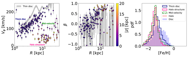
Figure 15: Chemo-kinematic analysis of the unclassified subsample (see Section  3.3 and Figure 5). Left: rotational velocity as function of the cylindrical radius, the grey bands show the GP-interpolation of the rotational velocities obtained for the rotating disc-like component (see Figure 12). Centre: anisotropy parameter as a function of the cylindrical radius. The color map in the left and middle panels indicates the median value of the absolute value of $z$, the points and the error bars indicate the median values, the 16th and 84th percentile correspondingly of the a-posteriori distribution obtained for each bin. Right: metallicity distribution for the SOS stars in the unclassified subsample, the unfilled blue histogram contains the unclassified stars with thick-disc like kinematics, the unfilled magenta histogram shows the distribution for unclassified stars with halo like kinematics while the unfilled dashed-green histogram contains unclassified stars in bins with intermediate azimuthal velocity ($\approx 100\ \,{\rm km\,s}^{-1}$). As comparison, the blue and red filled histograms show the metallicity distribution of the stars belonging to the the halo-like and disc-like components (see Section  3.3 and Figure 14). The metallicities shown in this figure have been estimated through Equations 3 and 4 (see Appendix A).

Additionally, beyond $R>10$ kpc and $|z|>10$ kpc above the plane, another barely rotating population is discernible - most likely belonging to the halo. There is also a small number of bins that display kinematical properties in between the thick disc and the halo. Interestingly, the halo portion of the unclassified RRL exhibit high orbital anisotropy $\beta\approx 0.8$ as evidenced in the middle panel of Figure 15. This would imply that much of this halo substructure is attributable to the Gaia Sausage. This is in agreement with the earlier claims of Simion et al. (2019) who connect the Virgo Overdensity and the Hercules Aquila Cloud to the same merger event. In fact, in Figure 5, traces of both the VOD and the HAC are visible amongst the unclassified RRL stars. Note that assigning the slowly-rotating portions of the halo to the GS debris cloud would increase the net angular momentum of this radially-biased halo component. The bins dominated by the thick disc stars have $\beta\approx 0$ with a mild increase with radius $R$. It is curious to see that the slowly rotating RRL population is limited to $R<12$ kpc as has been seen in many previous studies (e.g. Bovy et al., 2012; Hayden et al., 2015; Bland-Hawthorn et al., 2019; Grady et al., 2020) supporting the picture where rather than just thick, this is an inner, old disc of the Galaxy.

The right panel of Figure 15 presents the metallicity distributions of the halo (unfilled magenta), thick disc (unfilled blue) and intermediate $v_{\phi}$ (green dashed) populations amongst the previously unclassified RRL. These can be compared to the halo (filled light red) and thin disc (filled light blue) [Fe/H] distributions. Reassuringly, the bits of halo substructure with slight prograde motion have the [Fe/H] distribution indistinguishable from the that of the halo’s sample. The thick disc displays metallicities that are on average lower than the thin disc’s but not as low as in the halo. Based on the chemo-kinematic trends amongst the ‘unclassified’ stars, we conclude that the majority $\approx 70\%$ belong to the Milky Way’s thick disc, while the remaining $\approx 30\%$ are part of the halo substructure, which displays the prevalence for prograde motion and high orbital anisotropy.

6.2 Tests and caveats

The results of this work rely on a number of assumptions. In this section we quantify the impact of some of the possible systematics, repeating the analysis of the halo and the disc kinematics (see Section  3.1, Section 4 and Section 5).

One of the principal ingredients of our modelling is the distance estimate for the RRL stars in our sample. We investigate the role of a potential distance bias using the SOS metallicity estimate instead of the one presented in this paper in Equation  3 and Equation  4 (see Appendix A). Moreover, we test the effect of assuming a constant absolute magnitude, $M_{\mathrm{G}}=0.64\pm 0.24$ (see Appendix A), in Equation  5. We are happy to report that all main conclusions of our analysis remain unchanged. The radial profile of the fitted halo and disc properties are all within 1$\sigma$ of our fiducial results and we do not find any significant systematic differences between the outcomes.

The separation of the halo and disc component relies on a selection cut based mainly on the a-posteriori likelihood to belong to the non-rotating halo component (see Section‘3.3). We do not repeat the kinematic analysis for different $q_{\mathrm{halo}}$-thresholds, but looking at Figure 15 the result of such an experiment is easily extrapolated. Increasing the value of the disc $q_{\mathrm{halo}}$-cut we include more and more of thick disc stars (that are larger in number) lowering the rotational velocity, increasing the velocity dispersion and lowering the metallicity. This does not change our conclusions but just hides the subdominant thin-disc-like component under a large number of stars belonging to a different kinematic component.

Part of the halo analysis relies on splitting the stars into spherical bins, however, the inner stellar halo is known to be flattened (see e.g. Deason et al. 2011; Xue et al. 2015; Das & Binney 2016; Iorio et al. 2018; Iorio & Belokurov 2019). We repeat the kinematic fit of the halo subsample using elliptical bins instead, tuned on the ellipsoidal shape described in Iorio & Belokurov (2019). Comparing the outcomes of the spherical and elliptical analysis we do not find any significant differences. Moreover, we perform an alternative analysis binning the volume in cylindrical coordinates, so that the results are independent on the assumption of spherical or elliptical symmetry (but still dependent on the azimuthal symmetry, see below). The results of the cylindrical analysis are qualitatively in agreement with the 1D radial profile obtained assuming spherical symmetry (see Figure  7 and Figure  8).

We test the assumption of the four-fold symmetry repeating our analysis considering only stars located in a given Galactic quadrant, i.e. we select stars based on their Galactic azimuthal angle. We do not detect any significant difference or systematic offset in the fitted halo and disc parameters (within 1$\sigma$ of our fiducial results), except for the azimuthal velocity of the radial component of the halo (see Section  4.1). This parameter shows a significant offset depending on the considered quadrants: in the Galactic semi-plane not containing the Sun ($90^{\circ}<\Phi<270^{\circ}$), the average azimuthal velocity is negative ($V_{\phi,\mathrm{rad}}\approx-25\ \,{\rm km\,s}^{-1}$), while in the other portion of the Galaxy $V_{\phi,\mathrm{rad}}$ is just slightly higher than 0, except in the innermost part where it rises up to $30-40\ \,{\rm km\,s}^{-1}$. The final velocity profile showed in Figure 8 is approximately the weighted mean (there are more stars in the quadrants closer to the Sun) of the $V_{\phi,\mathrm{rad}}$ profiles obtained considering the four different quadrants. Although we cannot exclude the presence of real asymmetries or hidden halo subcomponents, it is more likely that this difference is driven by the distance biases present (see e.g. Schönrich et al. 2011, 2012). Indeed, the velocity offset is dependent on the distance from the Sun with more distant quadrants showing a larger deviation from $V_{\phi,\mathrm{rad}}=0$. Curiously, the velocity offset is not present in the isotropic component, however $V_{\phi,\mathrm{iso}}$ is in general less constrained. In that case, the random errors are likely dominating the error budget reducing the effect of the systematic offset.

The results for the thin disc are obtained assuming isotropy, hence we repeat the fit leaving the three components of the velocity ellipsoid free ($\sigma_{\mathrm{R}},\sigma_{\mathrm{z}},\sigma_{\mathrm{\phi}}$). We also model the non-diagonal terms of the correlation matrix as nuisance parameters. The results are consistent with those shown in Figure 12, in particular the three velocity dispersions agree within the errors confirming that our assumption of isotropy is supported by the data. However, we do expect a certain degree on anisotropy in the disc ($\sigma_{\mathrm{R}}>\sigma_{\mathrm{z}}$, see e.g. Sharma et al. 2020; Gaia Collaboration et al. 2018c). The reason why we do not detect the velocity dispersion anisotropy in our data is unclear. It is possible that we are introducing some selection bias in the kinematic decomposition (Section  3.3) as we force the rotating component to be isotropic. It could also be that the differences are washed out by the noise in our data and by the limitation of our analysis. In particular, most of the stars in the rotating subsample have small $z$ (see Figure 5), hence $V_{b}$ is almost directly mapping $V_{\mathrm{z}}$ while the other two velocity components are harder to constrain. Despite this possible issue about the velocity dispersion, the model parameters of the rotating component (azimuthal velocity and velocity dispersion, see Section  5) are relatively insensitive to any of the tested variations, therefore the association of this component with the kinematic thin disc is robust.

Concerning the chemical analysis it is important to stress that it is based on photometric metallicities (see Appendix A). As already noted by Clementini et al. (2019) and Cacciari et al. (2005), such photometric estimates are not suited to describe individual metallicities but rather the average metal abundance of a population. Moreover, as shown in Figure 14, the photometric metallicity can differ significantly between different calibrations. Most of our analysis is based on the comparison between metallicity distributions of groups of stars (see Figure 10 and Figure 14), hence the results should be robust despite the limitation imposed by the use of photometric metallicities. Concerning the rotating disc-like component it is evident that the metallicity is on average higher with respect to the halo. However, given the uncertainty of the photometric metallicities it is hard to constrain the real average metallicity of this population. As discussed in Appendix A, we notice that our photometric estimate seems to underestimate high metallicities, on the contrary the metal abundance reported in the SOS catalogue tends to overpopulate the high metallicity end of the [Fe/H] distribution. Therefore, we conjecture that the true average value is somewhere between our estimate ([Fe/H]$\approx-1$) and the higher value estimated in the SOS catalogue ([Fe/H]$\approx-0.4$). Interesting, we notice that the high resolution spectroscopic datasample of field RRL from Magurno et al. (2018) shows a clear metal-rich component, ranging between [Fe/H]$\approx-0.5$ and [Fe/H]$\approx 0.2$, in the metallicity distribution (see Figure 12 in Fabrizio et al. 2019 and Figure 17 in Appendix A.)

Recently, Beraldo e Silva et al. (2020) pointed out that our comparison with the Sharma et al. (2020) models could be biased toward younger age because our sample is kinematically selected. However, we stress that the Sharma et al. (2020) models take into account the kinematics through the vertical angular momentum parameter, $L_{\mathrm{z}}$. Indeed, at a given age, they predict smaller velocity dispersions for larger $L_{\mathrm{z}}$, this is an expectation of the model not an effect of a selection bias. It is important to note that in our case we can associate $L_{\mathrm{z}}=V_{\phi}R$ to each star in a bin (see Fig. 13), so the selection on $V_{\phi}$ (selecting small $q_{\mathrm{halo}}$) as well on $z$ (see Eq. 11) are not introducing any bias since they are both parameters of the Sharma et al. (2020) models and the only free parameters of our analysis is the population age.

Beraldo e Silva et al. (2020) conclude that the presence of a population of old RRL in the thin disc can be easily accommodate considering an early co-formation of thin and thick discs. This can surely be the case, but we stress once again that the progenitors of metal-rich RRL ([Fe/H]$>-1$) need a significant mass loss to reach the instability strip regardless of their age.

6.3 The bulge/bar

The closest the stars in our sample get to the Galactic centre is $\approx 1.3$ kpc. Combined with the restriction on the dust reddening which eliminates low latitudes, this implies that the Milky Way’s bar and bulge are mostly excluded from our study. As of today, OGLE (e.g. Soszyński et al., 2014) and VVV (Dékány et al., 2013) surveys provide much better view of the RR Lyrae properties in the heart of our Galaxy. The structure and the metallicity distribution of the bulge region as traced by RR Lyrae appear complex and puzzling and agreement is yet to be reached as to the exact interplay of distinct Galactic components here (Pietrukowicz et al., 2015; Kunder et al., 2016; Dékány et al., 2018; Prudil et al., 2019a, c; Kunder et al., 2020; Du et al., 2020). The bulge tangled mess might well have reached into our sample for stars with distances $R<4$ kpc from the Galactic centre, but their numbers are low and their (potential) contribution does not change any of the conclusions reported here.

6.4 Conclusions

We use Gaia DR2 proper motions to identify individual Galactic components amongst RRL, pulsating horizontal branch stars, usually assumed to be mostly old and metal-poor. Following the ideas recently highlighted in Wegg et al. (2019), we assume four-fold symmetry to extract the properties of the 3D velocity ellipsoid as a function of Galactocentric distance $R$ and height $|z|$. The Gaia DR2 RRL catalogue is dominated by stars with halo kinematics ($\approx 70\%$), i.e. those with little prograde rotation. Some $\approx 5\%$ of the RR Lyrae have fast azimuthal velocities, $v_{\phi}\approx 220-230$ kms^-1, while the remaining $\approx 25\%$ are unclassified, i.e. have kinematic properties intermediate between the halo and the thin disc. We further demonstrate that the halo sample contains at least three distinct sub-populations. The unclassified sample is dominated by the thick disc stars with a small addition of a mildly prograde halo debris.

Between 50% and 80% of the halo RRL stars with $5<R$(kpc)$<25$ belong to the radially biased ($\beta\approx 0.9$) non-rotating (or perhaps slowly rotating) structure known as the Gaia Sausage, left behind by an ancient merger with a massive dwarf galaxy (see e.g. Deason et al., 2013; Belokurov et al., 2018b; Haywood et al., 2018; Deason et al., 2018; Helmi et al., 2018; Mackereth et al., 2019a; Lancaster et al., 2019; Fattahi et al., 2019). The remainder of the halo is much more isotropic and probably contains a mixture of stars accreted from lower-mass satellites. The Gaia Sausage component exhibits little angular momentum and a strong bimodality in the radial velocity (see Lancaster et al., 2019; Necib et al., 2019). We model the radial velocity distribution of the Gaia Sausage with two Gaussians separated by $2L_{r}$ and show that the amplitude of the radial velocity separation is a strong function of the Galactocentric distance $R$. $L_{r}$ peaks around $3<R$(kpc)$<5$, the distance, we conjecture, which marks the location of the pericentre of the GS, while its apocentre is close to $R\approx 25$ kpc where $L_{r}$ drops to 0 kms^-1. The GS debris is distinct from the rest of the halo not only kinematically but also in terms of the lightcurve shapes of the constituent RRL. Compared to the isotropic halo, the GS RRL boast a higher fraction of Oosterhoff Type 1 objects. Beyond $R\approx 10$ kpc, the GS stars are more metal-rich than the isotropic halo, and additionally exhibit a higher fraction of the HASP RRL (in agreement with e.g. Belokurov et al., 2018a) supporting the massive merger scenario. However, within 10 kpc, there exists a subset of the isotropic halo RRL whose metallicity and HASP fraction is even higher than those in the GS. We conjecture that these inner metal-rich and HASP-rich RRL were born in situ (representing the population previously seen in e.g. Nissen & Schuster, 2010; Bonaca et al., 2017; Haywood et al., 2018; Di Matteo et al., 2019; Gallart et al., 2019; Belokurov et al., 2020a).

We are not the first to detect RRL stars with disc kinematics (see Kukarkin, 1949; Preston, 1959; Taam et al., 1976; Layden, 1994, 1995a, 1995b; Mateu & Vivas, 2018; Marsakov et al., 2018, 2019; Prudil et al., 2020; Zinn et al., 2020). Note however, that these previous studies have been mostly limited to the Solar neighborhood. Here for the first time we map out the kinematics of the disc RRL over the entire extent of the disc, i.e. $3<R$(kpc)$<30$. The RRL with the fastest azimuthal speeds in our sample follow closely the thin disc behaviour, both in terms of their rotation curve and the evolution of the velocity dispersion. Using the recent models of the velocity dispersion obtained for conventional thin disc tracers such as MS and RGB stars by Sharma et al. (2020) we place strong constraints on the typical age of the thin disc RR Lyrae. The thin disc traced by the Gaia RRL is very cold and can not be more than $\approx 5$ Gyr old. Moreover, we demonstrate that the thin disc RRL ought to be significantly more metal-rich compared to their halo counterparts, in agreement with the earlier studies mentioned above. The thick disc RRL are also detected as part of our study. These stars do not rotate as fast and hence are placed in the “unclassified” category. Careful examination of these stars with intermediate kinematic properties reveal that in bulk, they are denizens of the thick disc. Their lightcurve shapes indicate that they only slightly more metal-rich compared to the halo. Curiously, the kinematically-selected thick disc RRL do not tend to reach beyond 10-12 kpc from the Galactic centre, in agreement with the theories of the thick disc formation.

We draw attention to the fact that the existence of young and metal-rich RRL stars in the thin disc can not be easily reconciled with the predictions of the accepted, single-star evolutionary model: metal-rich young progenitors require un-physically high mass loss. Perhaps, instead we have discovered an army of RR Lyrae impostors (akin to BEPs) produced via mass transfer in binary systems.

Data Availability

The data underlying this article are available in Zenodo at http://doi.org/10.5281/zenodo.3972287.

Appendix A Photometric metallicity estimate

Most of the stars in the SOS Gaia catalogue have photometric metallicities (Clementini et al., 2019) estimated through the non-linear relation by Nemec et al. (2013). The Nemec et al. (2013) relation has been fitted to a small sample of stars and it does not seem to generalise well enough on larger sample. In particular, it assigns to a group of RRL with intermediate-large periods and large $\Phi_{31}$ high metallicities ($[Fe/H]\gtrsim-0.5$) that are likely artefacts (see e.g. Fig. 17). Moreover, the relation is based on the Kepler magnitude band and a number of auxiliary relations have to be used to translate the $\Phi_{31}$ from the original band to the Gaia one (Clementini et al., 2019); additionally the value of $\Phi_{31}$ can change if we use a different number of harmonics to decompose the light curve. For all these reasons, we decide to find a relation based solely on the light curve properties reported in the Gaia SOS catalogue. For the purpose of our analysis we cross-matched the subsample of RRab stars with complete SOS light curve information in our Gclean catalogue (see Sec. 2) with different spectroscopic sample of RRab stars with spectroscopic metallicity estimate: Layden (1994) (84 stars), Marsakov et al. (2018) (76 stars), Nemec et al. (2013) (21 stars), Zinn et al. (2020) (149 stars, mostly based on the sample by Dambis et al. 2013 containing also the 84 stars in Layden 1994). Concerning the RRc stars we follow Nemec et al. (2013) considering the RRL in globular clusters (50 stars) assigning them the metallicity of the cluster they belong. We use the catalog of Gaia objected associated with Globular Clusters in Gaia Collaboration et al. (2018d), while the Globular Cluster metallicity are taken from Harris (1996). We consider the old Harris (1996) compilation because the metallicities are reported in the Zinn & West (1984) metallicity scale instead of the Carretta et al. (2009) scale used in the more recent Harris (2010) catalogue. The Zinn & West (1984) scale is the same metallicity scale of spectroscopic catalogs and the absolute magnitude-metallicity relation used in this work has been calibrated on this same scale (Muraveva et al., 2018).

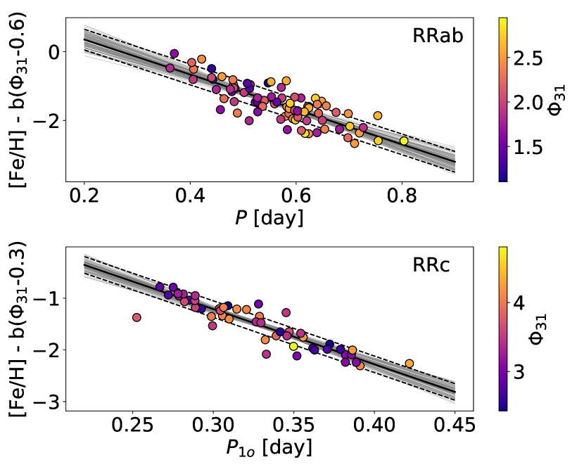
Figure 16: Best fit linear relation $[Fe/H]\propto a\times~{}P+b\times\Phi_{31}$ for RRab (top panel) and RRc stars (bottom panel). The spectroscopic metallicities are from Layden (1994) and Harris (1996) for RRab and RRc stars, respectively. Periods and phase difference $\Phi_{31}$ values are from the SOS Gaia catalogue. The solid black lines show the median of the posterior distributions of the relations, while the gray lines are randomly sampled from the same distributions. The black dashed lines indicate the intrinsic scatter. The best fit relations are given in Equations 3 and 4.

We perform a large number of tests using both linear (e.g. Jurcsik & Kovacs 1996; Smolec 2005) and non linear relations (e.g. Nemec et al. 2013) and investigating different combinations of light curve and stellar properties. Initially, we evaluate the feature relevance through a random forest regression of the metallicity using the scikit-learn python module (Pedregosa et al., 2011). In practice we consider as feature: the period $P$ (fundamental period for RRab and first overtone period for RRc), the phase difference between the third or second light curve harmonics with respect to the fundamental one, the amplitude, the ratio between the amplitude of third or second light curve harmonics with respect to the fundamental one and the stellar color. In order to check possible biases and artefacts we also add the number of Gaia observations, the mean $G$ magnitude and the $RUWE$ to the group of features. For both RRab and RRc samples the most relevant feature is by far the period $P$, followed by the phase difference $\Phi_{31}$. We do not use the random forest method to estimate the metallicity since our training sample is relatively small and, considering the large number of parameters involved, it is very likely to produce a significant variance or overfit problem. Instead we fit the relations using a Bayesian approach taking into account the uncertainties of all the used features. In each tested relation we consider also the presence of an intrinsic scatter. We sample the posterior of the relation parameters exploiting the Hamiltonian MCMC technique making use of the python module PYMC3 (Salvatier et al., 2016). The performance of the various relations are analysed considering: $i$) fit residuals, $ii$) comparison with metallicities of RRL stars in Globular clusters (association with GC from Gaia Collaboration et al. 2018d, metallicites estimate from Harris 1996), $iii$) comparison with the spectroscopic metallicities of the RRL stars in the solar neighbours,the halo and the bulge taken from the crossmatch with the Magurno et al. (2018), Liu et al. (2020) and Savino et al. (2020) samples (see Fig. 17), $iv)$ comparison of the distance moduli derived using the $M_{G}-[Fe/H]$ relation by Muraveva et al. (2018) with the distance moduli of the Magellanic Clouds. We conclude that the optimal fit, both for RRab and RRc stars, is obtained with a linear relation with $P$ and $\Phi_{31}$, very little improvements can be obtained using non-linearity or adding parameters to the relation. As already noted by Jurcsik & Kovacs (1996); Smolec (2005); Nemec et al. (2011), the major issue is a moderate systematic trend of the residuals as a function of the spectroscopic metallicities: the relation tends to overestimate (underestimate) the metallicity at the metal-poor (metal-rich) end. Anyhow, this problem is present with the same significance also with more complex models. This is likely due to the lack of calibrators at both ends of the metallicity distribution. Among the various samples of RRab, the results of the fit are very similar except for the Nemec sample, but it contains a small number of stars covering a narrower range of metallicites with respect to the other samples. Therefore, we adopt as final relations (Equation 3 and 4), the linear relation in $P$ and $\Phi_{31}$ obtained with the Layden (1994) sample (for RRab stars). This choice is motivated by the fact that it is not a collection of different catalogues and it reports a metallicities uncertainty for each star. Fig. 16 shows the best-fit relations. The metallicity interval of the fit training set ranges from -2.51 to 0.08 for the RRabs stars and from -2.37 to -0.55 for the RRc stars. Only a very small portion (mostly RRc stars) of our Gclean sample (see Sec. 2.2) has metallicities extrapolated outside these ranges: 396 at the metal-poor tail (93 RRab, 303 RRc, 295 in the halo subsample, 6 in the disc subsample), 105 at the metal-rich end (26 RRab, 79 RRc, 15 in the halo subsample, 42 in the disc subsample). These numbers are small enough to have negligible effects on our outcomes as confirmed by the results obtained with the SA sample (see e.g. Fig. 12 and Fig. 7) that contains only $0.3\%$ of stars with extrapolated metallicities. Moreover, the fit procedure “naturally" assigns larger errors to extrapolated metallicities and the implemented linear function limits uncontrolled behaviour outside the range of calibrators.

Compared to the photometric metallicities reported in the Gaia SOS catalogue our estimate perform better both on estimating the absolute magnitude of the stars in the Magellanic Clouds (using the $M_{G}-[Fe/H]$ relation by Muraveva et al. 2018) and compared to the RRL sample of spectroscopic metallicity obtained by Savino et al. (2020), Liu et al. (2020) and Magurno et al. (2018). Fig. 17 shows that the distribution of SOS photometric metallicities significantly differs from the spectroscopic ones in both shape and centroid position (see also Hajdu 2019). In particular, considering the bulge sample, the SOS distribution peaks at a very metal-rich value of $[Fe/H]\approx-0.5$, while the peak of the spectroscopic metallicity is $[Fe/H]\approx-1.5$. The photometric metallicity estimated with our relation shows a more similar distribution with a coincident but narrower peak. The narrow distribution of the photometric metallicities is due to the already discussed problem of overestimating/underestimating the metallicities at the edge of the distribution. Considering the Liu et al. (2020) sample, our metallicity distribution is slightly offset from the spectroscopic distribution, but overall the distribution widths are very similar. On the contrary, the SOS distribution is much more spread containing a significant number of metal-rich stars ($[Fe/H]>-1$). The peak of the distribution of our photometric metallicities is consistent with the peak of the high resolution spectroscopic metallicities in Magurno et al. (2018), but in this case the differences in the tails are more significant. For the same sample, the SOS photometric metallicities cover the same range of the spectroscopic metallicities, but their distribution is much flatter without a clear peak and with an over-abundance of very metal-rich stars.

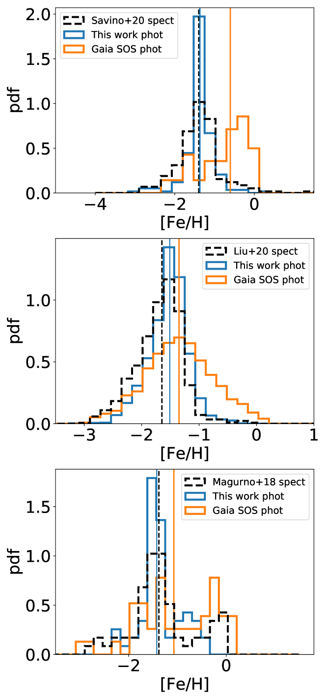
Figure 17: Comparison between the distribution of photometric (this work, blue; Gaia SOS orange) and spectroscopic (dashed-black) metallicity values for two samples of RRL. Top panel: cross-match between the bulge RRL sample in Savino et al. (2020) and Gaia SOS with lightcurve information (212 stars). Middle panel: cross-match between the RRL sample (mostly in the halo) from Liu et al. (2020) and Gaia SOS with lightcurve information (3153 stars). Bottom panel: cross-match between the RRL sample (local field) from Magurno et al. (2018) and the Gaia SOS with lightcurve information (64 stars). Vertical lines indicate the median of each distribution.

Finally, we test that the use of the constant absolute magnitude $M_{G}=0.64\pm 0.25$ for both RRab and RRc stars (see e.g. Iorio & Belokurov 2019) is a good approximation when light curve properties are not available.The associated error $\delta M_{G}=0.25$ is a robust and conservative estimate that can absorb both random and systematic uncertainties (e.g. RRL type, metallicity) giving a error on heliocentrinc distance of about $13\%$.

Appendix B Rotation Matrix

The rotation matrix $\mathbf{R}$ to pass from velocities in Spherical $\bm{V}_{\mathrm{sph}}=(V_{\mathrm{r}},V_{\mathrm{\theta}},V_{\mathrm{\phi}})$ or Cylindrical $\bm{V}_{\mathrm{cyl}}=(V_{\mathrm{R}},V_{\mathrm{z}},V_{\mathrm{\phi}})$ Galactocentric coordinates to the velocities in the observed frame of reference $\bm{V}_{\mathrm{sky}}=(V_{\mathrm{los}},V_{\ell},V_{b})$ can be obtained with the matrix product

$$\mathbf{R}=\mathbf{R}_{\mathrm{c}}\cdot\mathbf{R}_{\mathrm{s,sph/cyl}}$$ (12)

where $\mathbf{R}_{\mathrm{c}}$ is the rotation matrix to pass from the Galactic cartesian velocities $\bm{V}_{\mathrm{car}}=(V_{\mathrm{x}},V_{\mathrm{y}},V_{\mathrm{z}})$ to the the observed velocities, while $\mathbf{R}_{\mathrm{s,sph}}$ and $\mathbf{R}_{\mathrm{s,cyl}}$ are the rotation matrix to pass from Galactic cartesian velocities to Galactic spherical and cylidrincal velocities, respectively. The matrix $\mathbf{R}_{\mathrm{c}}$ is defined as

$$\mathbf{R}_{\mathrm{c}}=\begin{bmatrix}\cos b\cos\ell&\cos b\sin\ell&\sin b\\ -\sin\ell&\cos\ell&0\\ -\sin b\cos\ell&-\sin b\sin\ell&\cos b\end{bmatrix},$$ (13)

while the matrices $\mathbf{R}_{\mathrm{s}}$ are defined as

$$\mathbf{R}_{\mathrm{s,sph}}=\begin{bmatrix}\Gamma\cos\theta\cos\phi&-\Gamma\sin\theta\cos\phi&-\Gamma\sin\phi\\ \cos\theta\sin\phi&-\sin\theta\sin\phi&-\cos\theta\\ \sin\theta&\cos\theta&0\end{bmatrix}$$ (14)

and

$$\mathbf{R}_{\mathrm{s,cyl}}=\begin{bmatrix}\Gamma\cos\phi&0&-\Gamma\sin\phi\\ \sin\phi&0&-\cos\phi\\ 0&1&0\end{bmatrix}.$$ (15)

The factor $\Gamma$ is equal to 1 for a right-handed Galactocentric frame of reference or to -1 for a left-handed Galactocentric frame of reference (as the one used in this work). The angular coordinates $\theta$ and $\phi$ are the zenithal and azimuthal angle respectively, while $b$ and $\ell$ are the Galactic sky coordinates (see Sec. 2.1).

References

- Ablimit et al. (2020) Ablimit I., Zhao G., Flynn C., Bird S. A., 2020, arXiv e-prints, p. arXiv:2004.13768
- Amarante et al. (2020) Amarante J. A. S., Smith M. C., Boeche C., 2020, MNRAS, 492, 3816
- Amorisco (2017) Amorisco N. C., 2017, MNRAS, 464, 2882
- Antoja et al. (2018) Antoja T., et al., 2018, Nature, 561, 360
- Athanassoula (2005) Athanassoula E., 2005, MNRAS, 358, 1477
- Aumer & Binney (2009) Aumer M., Binney J. J., 2009, MNRAS, 397, 1286
- Aumer et al. (2016) Aumer M., Binney J., Schönrich R., 2016, MNRAS, 462, 1697
- Bacchini et al. (2019) Bacchini C., Fraternali F., Pezzulli G., Marasco A., Iorio G., Nipoti C., 2019, A&A, 632, A127
- Barbanis & Woltjer (1967) Barbanis B., Woltjer L., 1967, ApJ, 150, 461
- Barbuy et al. (2018) Barbuy B., Chiappini C., Gerhard O., 2018, ARA&A, 56, 223
- Bell et al. (2008) Bell E. F., et al., 2008, ApJ, 680, 295
- Belokurov et al. (2007) Belokurov V., et al., 2007, ApJ, 657, L89
- Belokurov et al. (2014) Belokurov V., et al., 2014, MNRAS, 437, 116
- Belokurov et al. (2017) Belokurov V., Erkal D., Deason A. J., Koposov S. E., De Angeli F., Evans D. W., Fraternali F., Mackey D., 2017, MNRAS, 466, 4711
- Belokurov et al. (2018a) Belokurov V., Deason A. J., Koposov S. E., Catelan M., Erkal D., Drake A. J., Evans N. W., 2018a, MNRAS, 477, 1472
- Belokurov et al. (2018b) Belokurov V., Erkal D., Evans N. W., Koposov S. E., Deason A. J., 2018b, MNRAS, 478, 611
- Belokurov et al. (2019) Belokurov V., Deason A. J., Erkal D., Koposov S. E., Carballo-Bello J. A., Smith M. C., Jethwa P., Navarrete C., 2019, MNRAS, 488, L47
- Belokurov et al. (2020a) Belokurov V., Sanders J. L., Fattahi A., Smith M. C., Deason A. J., Evans N. W., Grand R. J. J., 2020a, MNRAS, 494, 3880
- Belokurov et al. (2020b) Belokurov V., et al., 2020b, MNRAS, 496, 1922
- Bensby et al. (2003) Bensby T., Feltzing S., Lundström I., 2003, A&A, 410, 527
- Bensby et al. (2013) Bensby T., et al., 2013, A&A, 549, A147