Performance Improvement of Path Planning algorithms with Deep Learning Encoder Model

Abstract

Currently, path planning algorithms are used in many daily tasks. They are relevant to find the best route in traffic and make autonomous robots able to navigate. The use of path planning presents some issues in large and dynamic environments. Large environments make these algorithms spend much time finding the shortest path. On the other hand, dynamic environments request a new execution of the algorithm each time a change occurs in the environment, and it increases the execution time. The dimensionality reduction appears as a solution to this problem, which in this context means removing useless paths present in those environments. Most of the algorithms that reduce dimensionality are limited to the linear correlation of the input data. Recently, a Convolutional Neural Network (CNN) Encoder was used to overcome this situation since it can use both linear and non-linear information to data reduction. This paper analyzes in-depth the performance to eliminate the useless paths using this CNN Encoder model. To measure the mentioned model efficiency, we combined it with different path planning algorithms. Next, the final algorithms (combined and not combined) are checked in a database that is composed of five scenarios. Each scenario contains fixed and dynamic obstacles. Their proposed model, the CNN Encoder, associated to other existent path planning algorithms in the literature, was able to obtain a time decrease to find the shortest path in comparison to all path planning algorithms analyzed. the average decreased time was 54.43%.

1

I Introduction

Path planning algorithms are essential for the accomplishment of many activities in different areas, for example, robot navigation [1], path apps for locomotion in cities (for pedestrian and driver) [2], autonomous-driver cars [3]. These algorithms have different approaches to treat spatial information, the most used in the literature are, Grid-based search (which transforms the environment in a grid-mesh) [4], Interval-based search (similar to grid-based search it but uses space data instead of a grid) [5] and Reward-based (similar to a reinforcement learning in deep learning) [6].

Based on Grid-based search, the first path planning algorithm was proposed by Dijkstra in 1956. Although this solution is always able to find the shortest path between two points, Dijkstra’s algorithm has become obsolete because it has very high computational complexity. Considering the response time of the Dijkstra algorithm, it would be infeasible to be applied in many scenarios.

Given this problem, new algorithms with different approaches were created to improve performance in finding the shortest path between two points.

Since Dijkstra’s proposal, many algorithms have been created being able to find the shortest path with the lowest computational cost. A* [4], Bi A* [7], Breadth-first [8], Best-First [9] are a few of the search algorithms that exist for path planning. They have peculiarities that tackle different problems, and, therefore, are useful and important in many areas. These algorithms, however, become extremely costly when applied to large environments or environments with dynamic objects [10]. All these algorithms are detailed in the theoretical foundation section II-A.

The problem of the increased computational cost when increasing the amount of information is a problem that affects several fields of research, for example, pattern recognition [11], computer vision [12], text mining [13]. A very well-known approach to avoid this problem is to reduce dimensionality by discarding irrelevant information to the task.

Principal component analysis (PCA) is a mathematical procedure based on orthogonal transformation to convert data into a set of values of linearly unrelated variables called principal components. The number of principal components is always less than or equal to the number of original variables [14].

Truncated Singular value decomposition (TSVD) This algorithm use means of TSVD to performs linear dimensionality reduction. Differently of PCA, this solution does not center the data before computing the singular value decomposition [15].

Non-negative matrix factorization (NMF) Creates two non-negative matrices (W, H). The product of these matrices is an approximation of the non-negative input data. This method is used for dimensionality reduction [16].

These solutions significantly reduce dimensionality, keeping enough information to accomplish some tasks. However, a limitation of these approaches is since they reduce dimensionality using only linear correlation [17]. Therefore, in [18], the authors built a deep learning model able to reduce dimensionality using non-linearity correlation, named Convolutional Neuronal Network (CNN) Encoder. Their method removes mostly the useless information of the input data, including in dynamic environments. Eliminate useless information for path planning problem means to remove the paths which do not connect the start point and the goal point.

In this work, we perform an in-depth evaluation of the application of their proposed CNN Encoder to decrease the time spent by different path planning algorithms, showing the efficiency of the proposal to improve various path planning solutions.

II Material and Methods

II-A Theoretical Foundation

II-A1 Dijkstra’s algorithm

The Dijkstra’s algorithm proposed in 1956 by Edsger W. Dijkstra [19] is a path planning algorithm based on graph search. It solves the single-source shortest path problem for a graph with non-negative edge path costs, producing a shortest-path tree, it can be defined as follows:

Result: H, dist

initialization;

for each vertex $v$ in $V_{G}$ do

       $dist_{v}\leftarrow\infty$;

       $parent_{v}\leftarrow NIL$;

      

end for

$dist_{s}\leftarrow 0$;

while $Q\neq\emptyset$ do

       $u\leftarrow ExtractMin(Q)$;

       for each edge $e=(u,v)$ do

             $dist_{v}\leftarrow\infty$;

             if $dist_{v}>dist_{u}+weight_{e}$ then

                   $dist_{v}\leftarrow dist_{u}+weight_{e}$;

                   $parent_{v}\leftarrow u$

             end if

            

       end for

      

end while

$H\leftarrow(V_{G},\emptyset)$;

for each vertex $vinV_{G},\ v\neq s$ do

       $E_{H}\leftarrow E_{H}\cup\{(parent_{v},v)\}$;

      

end for

return $H,dist$

Algorithm 1 Dijkstra’s algorithm

II-A2 A *

The A* algorithm [20] was proposed to solve the limitations of Dijkstra’s algorithm, and to overcome it in the time spent to find the shortest path. This solution uses heuristics to be faster. It is defined as:

Result: $Shortest\ path$

$closedset\leftarrow\emptyset$;

$openset\leftarrow start$;

$camefrom\leftarrow emptymap$;

$gscore[start]\leftarrow 0$;

$fscore[start]\leftarrow g\ score[start]+heuristic\ cost\ estimate(start,goal)$;

while $openset\neq\emptyset$ do

       $current\leftarrow the\ node\ in\ openset\ having\ the\ lowest\ fscore\ value$;

       if $current=goal$ then

             return $Reconstruct\ Path(came\ from,goal)$;

            

       end if

      $remove\ current\ from\ openset$;

       $add\ current\ to\ closedset$;

      

      for $each\ neighbor\ in\ neighbor\ nodes(current)$ do

             if $neighbor\ in\ closedset$ then

                   $continue$;

                  

             end if

            $tentative\ g\ score\ \leftarrow g\ score[current]+distbetween(current,neighbor)$;

            

       end for

      if $neighbor\ not\ in\ openset\ or\ tentative\ g\ score\ <\ g\ score[neighbor]$ then

             $camefrom[neighbor]\leftarrow current$;

             $gscore[neighbor]\leftarrow tentativegscore$;

             $fscore[neighbor]\leftarrow gscore[neighbor]+heuristiccostestimate(neighbor,goal)$;

             if $neighbor\ not\ in\ openset$ then

                   $add\ neighbor\ to\ openset$;

                  

             end if

            return $failure$

       end if

      

end while

Algorithm 2 A* algorithm

II-A3 Bi A*

Bidirectional A* search is a graph search algorithm that finds the shortest path from an initial vertex to a goal vertex in a directed graph running two simultaneous searches [7]. It can be described as:

Result: $H,dist$

$Astart1\leftarrow Astart(start,goal)$;

$Astart2\leftarrow Astart(goal,start)$;

while $Astart1.current\neq Astart2.current$ do

       $path\ one\leftarrow Astart1.run()$;

       $path\ two\leftarrow Astart2.run()$;

      

end while

$shortest\ path\leftarrow path\ one+path\ two$;

$H\leftarrow(shortest\ path)$;

return $H$

Algorithm 3 Bi A*

II-A4 Breadth-first

The Breadth-first Search [8] is a classic graph search algorithm, and it works by expanding and systematically exploring a given node and progressively redoing the same procedure for all its neighbors. At each iteration, the last one explored, but not expanded, or visited, is selected. Also, this algorithm discovers all nodes that are a certain distance from the start.

Input: $nodes,source$

Result: $tree$

$start\leftarrow{\{source\}}$;

$next\leftarrow{\{\}}$;

$parents\leftarrow{[-1,-1,...,-1]}$;

while $start\neq{\{\}}$ do

       for  $v\in start$ do

             for $n\in neighbors[v]$ do

                   if $parents[n]=-1$ then

                         $parents[v]\leftarrow v$;

                         $next\leftarrow next\cup\{n\}$;

                        

                   end if

                  

             end for

            

       end for

      $start\leftarrow{next}$;

       $next\leftarrow{\{\}}$;

      

end while

return $tree$

Algorithm 4 Breadth-first algorithm

II-A5 Best-First

Based on the different strategies for solving search problems, the Best-First [9] algorithm is one of the most popular in the literature. Given the heuristic function $F(n)=h(n)$, which is applied equally throughout the search space, the algorithm aims to use this to quantify the value of each candidate exploited during the process and, thus, continue the exploration until reach the point of interest.

Input: $Graph,start,goal$

$PriorityQueue\leftarrow{\{\}}$;

$PriorityQueue\leftarrow{start}$;

while $PriorityQueue\neq{\{\}}$ do

       $u\leftarrow removeMin(PriorityQueue)$;

      

      if $u=goal$ then

             $exit$;

       end if

      

      for $each\ neighbor\ v\ of\ u$ do

             if $v\ is\ unvisited$ then

                   $mark\ v\ as\ visited$;

                   $PriorityQueue\leftarrow{v}$;

                  

             end if

            

       end for

      $mark\ u\ as\ exploited$;

      

end while

Algorithm 5 Best-First algorithm

II-B Path Planning Database

Following the research of Janderson et al. previous work and thus demonstrating the efficiency of their proposal concerning the conventional approaches, we use the image database that was proposed by them, to expand previous results through the comparison with other solutions present in the literature. It contains various formats, distributed in five different scenarios. They have variations of start, goal points for each instance in the database; consequently, the possibilities of paths to be taken. In Figure 2, it is possible to see an instance of each scenario.

Using their database is possible to perform a more detailed analysis of the model’s ability to generalize its responses, as well as its level of efficiency when compared to other solutions in different scenario configurations. As mentioned before, their database contains five scenarios, where each one has a total of 10000 scenes, which are RGB images with a resolution of 60 x 60 pixels. The variation between them is due to the random positioning of obstacles; which simulates physical obstacles. Also, for each one of the images, there is a label, being a GrayScale 60 x 60 image, which contains the shortest path of the scene.

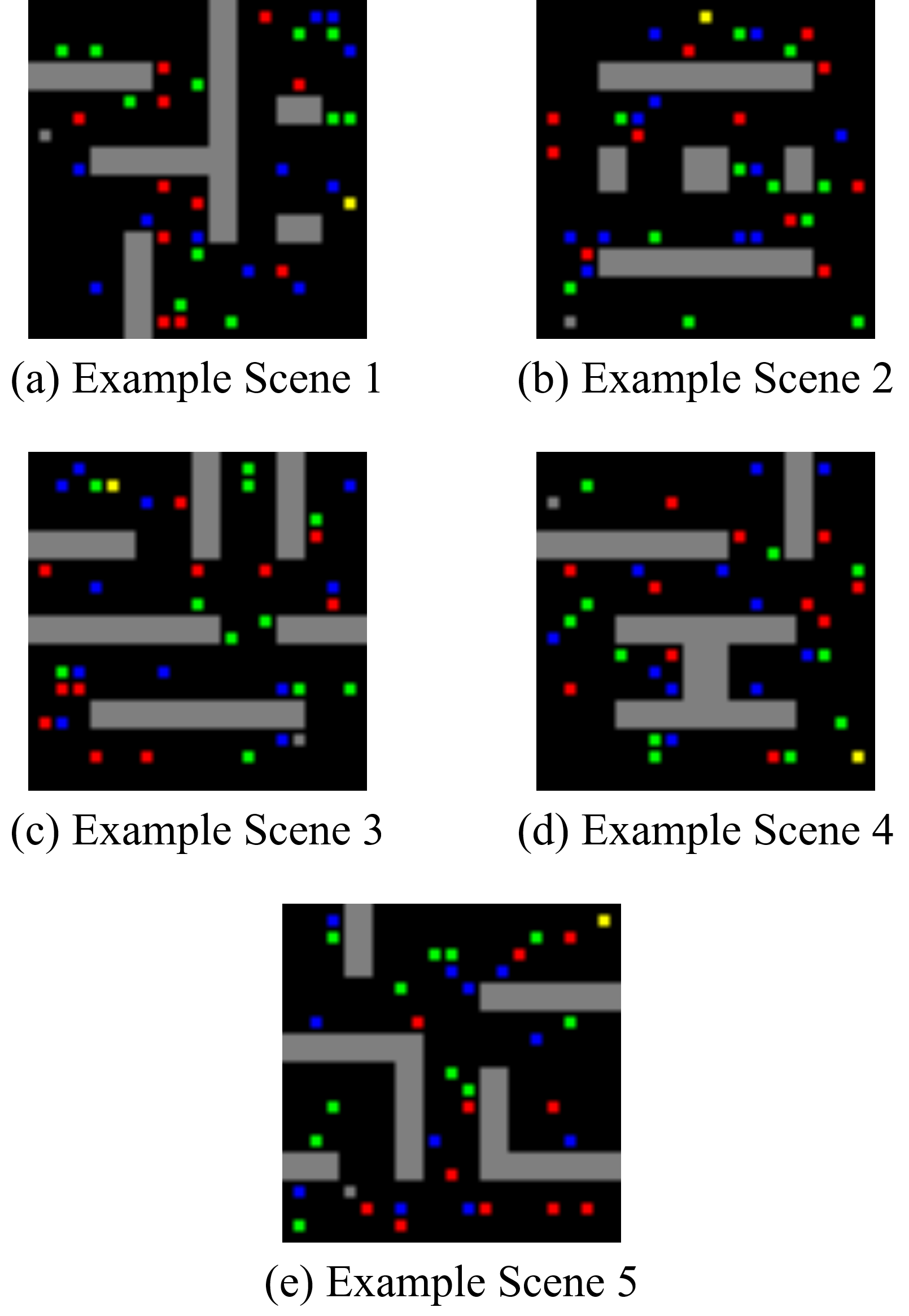
Figure 1: The instances of the used database. The yellow pixels represents the start and, the gray ones, the end of the path.

II-C The Convolutional Neural Networks Encoder

Autoencoders are being used to code data information in unsupervised learning [firstae]. They are trained to reconstruct the input data using fewer data than the original input; this way, many times, they can eliminate useless information. On the other hand, Convolutional Neural Networks has an excellent capability to extract high-level features in tasks of deep learning and computational vision problems[21]. Trying to get the best of each model, Janderson et al. built a CNN Encoder to reduce the dimensionality of the data. This solution can eliminate useless routes from 2D maps [18].

II-C1 The model architecture

The architecture used was obtained through a testing process, where its construction took place through adjustments based on the results generated. Finally, the architecture reached can be analyzed in Table I.

TABLE I: Architecture of the CNN Encoder

Layer		Filters	Kernel Size	Activation	Batch Norm	Dropout
1	Image	-	-	-	-	-
2	Conv	64	3x3	ReLu	True	-
3	Conv	128	3x3	ReLu	False	30%
4	Max-Pool	-	3x3	-	-	-
5	Conv	256	3x3	ReLu	True	-
6	Conv	512	3x3	ReLu	False	30%
7	Dense	256	-	LeakyReLU	True	30%
8	Dense	512	-	LeakyReLU	True	30%
9	Dense	1024	-	LeakyReLU	True	30%
10	Dense	3600	-	Tanh	False	30%

II-D Experimental Setup

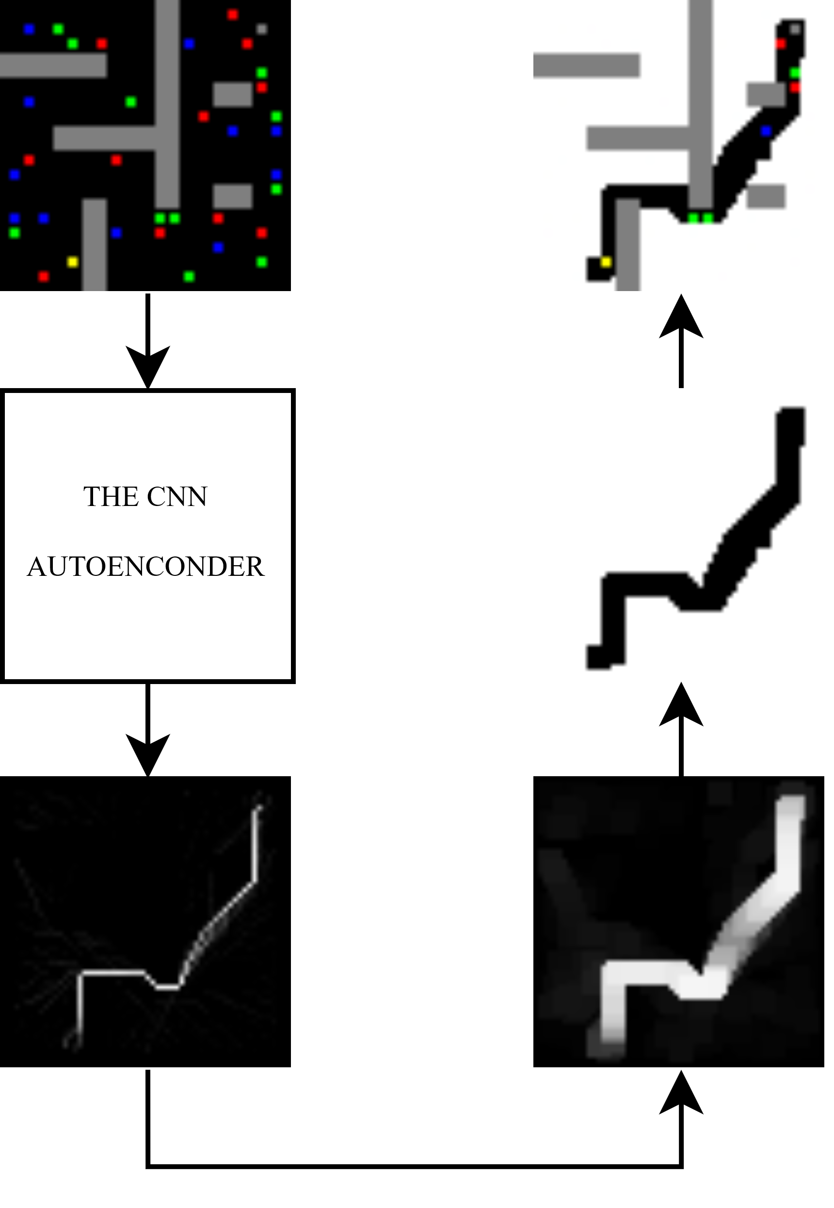
Figure 2: Representation of the processing applied to the output of CNN Encoder. Here it is possible to analyze that approach has achieved a considerable reduction in the search space. In both the first and the last stages of the process, the black pixels represent the walking paths for the search algorithm.

In this section, we describe the metrics used to evaluate the obtained results, how the database was manipulated, and the output processing. We also specify the hardware characteristics of the desktop computer used to perform the experiments; this is important because the hardware influences some experiments.

II-D1 Hardware Specification

The algorithms were written in python 3.7 and implemented in an Intel i5-8400 six-core, with a base frequency of 2.80GHz and 8GB of RAM. More details are depicted in Table II.

TABLE II: Specifications of the desktop computer used to run the experiments.

Model	Intel(R) Core(TM) i5-8400GHz
Number of Cores	6
Number of Threads	6
Base Frequency	2.80GHz
Cache Size	9MB
RAM	8GB

II-D2 Metrics

• Number of iterations. Represents the number of attempts until the algorithm found the shortest path.

• The path planning algorithm time. Represents the time in seconds that the algorithm spent to find the shortest path.

• CNN Encoder and preprocess output time. Represents the time in seconds that the CNN Encoder spent to predict the data input plus the time to preprocess it.

• Total time.

II-D3 Database Division

Percentage Split

• Train 80%

• Validation 10%

• Test 10%

III Experimental results

To evaluate this work, we applied the path planning algorithms mentioned in the theoretical foundation to the path planning database, and compare the average number of iterations when the CNN Encoder is combined or do not with these algorithms. Also, we compare the average of the time spent with and without using the proposal. The results were obtained using the test set (1000 images for each scene).

To facilitate the visualization of the results, they were compiled and divided into three tables. Table III shows the number of interactions of each algorithm for each scenario separately; this is important to analyze the model behaviour in different scenarios. Also, Table III shows the percentage of improvement between the algorithms when using or not using the model. On the other hand, Table IV shows the spent time of the algorithms to find the shortest path for each scenario. Also, the improvement time with and without the model was calculated.

In the conventional A* algorithm, we obtained an average improvement of 59.87% in terms of number of iterations. Looking at the execution time, with the application of the solution, we achieved an average improvement of 49.87%.

Going to the Best-First search algorithm, we achieved an average improvement of 53.87% in terms of number of iterations, also, in execution time, an average improvement of 16.06%.

Using a variation of the first tested algorithm, Bi A*, an average improvement of 56.12% was presented in terms of number of iterations, in the execution time, an average improvement of 40.88%.

We also used the Breadth-first algorithm, which is very widespread in the literature, we managed to achieve an average improvement of 83.77% in terms of number of iterations, in the execution time, an average improvement of 65.46%.

Finally, we applied the proposal to the Dijkstra algorithm, we obtained an average improvement of 84.12% in the number of iterations and looking at the execution time, there was an average improvement of 81.24%.

In Table V, it is possible to see a compilation of our results, containing a summary comparison between the standard execution of the search algorithms and their new results after the addition of our proposal. Also, it is possible to see some qualitative results in Figure 3.

TABLE III: Comparison between the number of iterations using only the path planning algorithms and the result after adding the CNN Encoder.

	Scene 1	Scene 2	Scene 3	Scene 4	Scene 5
A*	910.95	623.33	449.56	616.71	584.32
CNN Encoder + A*	301.42	246.70	221.70	254.06	254.07
Improvement	66.91%	60.42%	50.68%	58.80%	56.52%
Total Improvement	59.87%
Best-first	263.07	86.01	119.24	162.42	174.1
CNN Encoder + Best-first	93.45	75.64	63.15	67.69	71.34
Improvement	64.48%	12.05%	47.04%	58.32%	59.03%
Total Improvement	53.87%
Bi A*	946.31	491.44	458.24	665.34	499.88
CNN Encoder + Bi A*	341.61	254.85	227.30	272.18	247.39
Improvement	63.90%	48.14%	50.40%	59.09%	50.51%
Total Improvement	56.12%
Breadth-first	2268.59	2591.56	2188.41	2376.08	2286.77
CNN Encoder + Breadth-first	413.48	377.33	384.07	368.17	359.62
Improvement	81.77%	85.44%	82.45%	84.51%	84.27%
Total Improvement	83.75%
Dijkstra	2284.51	2669.13	2285.65	2405.46	2343.36
CNN Encoder + Dijkstra	413.82	377.70	384.33	368.38	359.83
Improvement	81.89%	85.85%	83.18%	84.69%	84.64%
Total Improvement	84.12%

TABLE IV: Comparison between the spent time using only the path planning and the result after adding the CNN Encoder.

	Scene 1	Scene 2	Scene 3	Scene 4	Scene 5
A*	0.027	0.021	0.013	0.018	0.017
CNN Encoder + A*	0.010	0.010	0.009	0.009	0.009
Improvement	61.25%	51.61%	28.79%	49.60%	46.13%
Total Improvement	49.87%
Best-first	0.009	0.003	0.004	0.005	0.005
CNN Encoder + Best-first	0.005	0.004	0.004	0.004	0.004
Improvement	34.94%	-50.54%	-1.42%	26.42%	24.96%
Total Improvement	16.06%
Bi A*	0.024	0.013	0.011	0.017	0.012
CNN Encoder + Bi A*	0.010	0.009	0.008	0.009	0.008
Improvement	55.08%	30.37%	26.83%	45.76%	30.87%
Total Improvement	40.88%
Breadth-first	0.013	0.015	0.013	0.014	0.013
CNN Encoder + Breadth-first	0.005	0.004	0.004	0.004	0.004
Improvement	60.81%	69.08%	62.42%	67.51%	66.69%
Total Improvement	65.46%
Dijkstra	0.043	0.056	0.045	0.049	0.048
CNN Encoder + Dijkstra	0.009	0.009	0.009	0.008	0.008
Improvement	77.07%	83.73%	79.57%	82.33%	82.54%
Total Improvement	81.24%

TABLE V: The average of time and interaction of all scenarios for each model

	Iterations	Time (s)
A*	636.97	0.0194748744
CNN Enconder + A*	255.59	0.0097622888
Best-first	160.98	0.0056170788
CNN Enconder + Best-first	74.25	0.00471486
Bi A*	612.24	0.0158272148
CNN Enconder + Bi A*	268.67	0.0093569152
Breadth-first	2342.28	0.0141633262
CNN Enconder + Breadth first	380.53	0.0048917796
Dijkstra	2397.62	0.0486876686
CNN Enconder + Dijkstra	380.81	0.0091321876

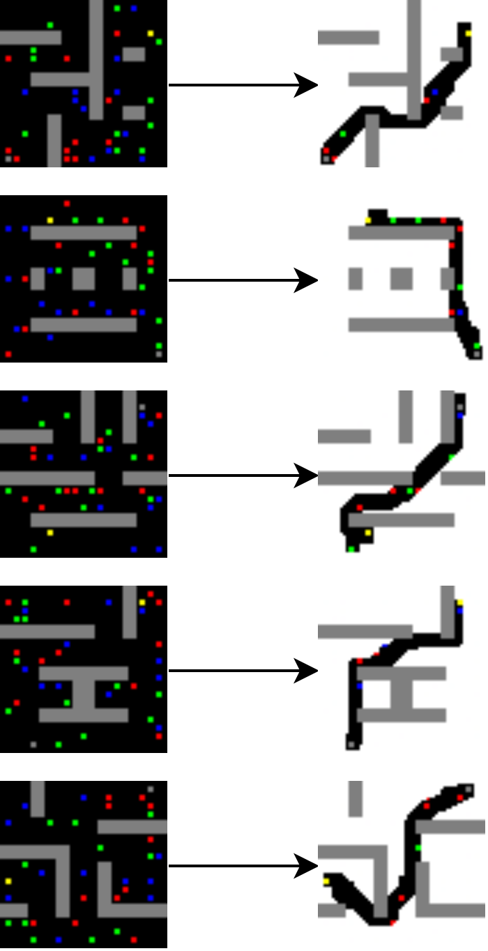
Figure 3: Comparison of the search space in an instance of each class, in the left column, the original scenes, in the right, the new search space after the application of the solution.

IV Conclusion

This work aimed to show that it is possible to improve the performance of path planning algorithms using a CNN Encoder to eliminate useless routes.

From the results obtained, we can assume that it is more advantageous to apply the CNN encoder to the existing path planning techniques. That is, the proposal was able to reduce the time to find the shortest path with all analyzed algorithms. In fact that CNN Encoder can eliminate routes in scenarios with fixed and dynamic obstacles, which may help in research with robotic navigation. As such, our contribution is to validate the architecture’s efficiency with different solutions from the path planning literature.

As future work, we hope to check the proposed model for the creation of a socially aware motion planning algorithm [22]. Also, we intend to combine new Deep Learning features with improving the architecture, which may reduce the response time even further.

References

- [1] Nayan M Kakoty, Mridusmita Mazumdar, and Durlav Sonowal. Mobile robot navigation in unknown dynamic environment inspired by human pedestrian behavior. In Progress in Advanced Computing and Intelligent Engineering, pages 441–451. Springer, 2019.
- [2] Yawei Pang, Lan Zhang, Haichuan Ding, Yuguang Fang, and Shigang Chen. Spath: Finding the safest walking path in smart cities. IEEE Transactions on Vehicular Technology, 68(7):7071–7079, 2019.
- [3] Meixin Zhu, Xuesong Wang, and Yinhai Wang. Human-like autonomous car-following model with deep reinforcement learning. Transportation research part C: emerging technologies, 97:348–368, 2018.
- [4] David Šišlák, Premysl Volf, and Michal Pechoucek. Accelerated a* trajectory planning: Grid-based path planning comparison. In 19th International Conference on Automated Planning and Scheduling (ICAPS), Thessaloniki, Greece, Sept, pages 19–23. Citeseer, 2009.
- [5] Andre Gaschler, Ingmar Kessler, Ronald P. A. Petrick, and Alois Knoll. Extending the knowledge of volumes approach to robot task planning with efficient geometric predicates. In 2015 IEEE International Conference on Robotics and Automation (ICRA). IEEE, may 2015.
- [6] I. Jeong, W. Ko, G. Park, D. Kim, Y. Yoo, and J. Kim. Task intelligence of robots: Neural model-based mechanism of thought and online motion planning. IEEE Transactions on Emerging Topics in Computational Intelligence, 1(1):41–50, Feb 2017.
- [7] Eric P Lafortune and Yves D Willems. Bi-directional path tracing. 1993.
- [8] Maciej Kurant, Athina Markopoulou, and Patrick Thiran. On the bias of bfs (breadth first search). In 2010 22nd International Teletraffic Congress (lTC 22), pages 1–8. IEEE, 2010.
- [9] Rina Dechter and Judea Pearl. Generalized best-first search strategies and the optimality of a. Journal of the ACM (JACM), 32(3):505–536, 1985.
- [10] MG Mohanan and Ambuja Salgoankar. A survey of robotic motion planning in dynamic environments. Robotics and Autonomous Systems, 100:171–185, 2018.
- [11] EFR Silva, LA Minho Cavalcante, AMP Santos Dos, WNL Santos Dos, et al. Screening of mangifera indica l. functional content using pca and neural networks (ann). Food chemistry, 273:115–123, 2019.
- [12] Thierry Bouwmans, Sajid Javed, Hongyang Zhang, Zhouchen Lin, and Ricardo Otazo. On the applications of robust pca in image and video processing. Proceedings of the IEEE, 106(8):1427–1457, 2018.
- [13] B Shravan Kumar and Vadlamani Ravi. Text document classification with pca and one-class svm. In Proceedings of the 5th International Conference on Frontiers in Intelligent Computing: Theory and Applications, pages 107–115. Springer, 2017.
- [14] Karl Pearson F.R.S. Liii. on lines and planes of closest fit to systems of points in space. The London, Edinburgh, and Dublin Philosophical Magazine and Journal of Science, 2(11):559–572, 1901.
- [15] Simon Du, Yining Wang, and Aarti Singh. On the power of truncated svd for general high-rank matrix estimation problems. 02 2017.
- [16] Daniel D. Lee and H. Sebastian Seung. Algorithms for non-negative matrix factorization. In Proceedings of the 13th International Conference on Neural Information Processing Systems, NIPS’00, pages 535–541, Cambridge, MA, USA, 2000. MIT Press.
- [17] H. Lu, K. N. Plataniotis, and A. N. Venetsanopoulos. Mpca: Multilinear principal component analysis of tensor objects. IEEE Transactions on Neural Networks, 19(1):18–39, 2008.
- [18] Janderson Ferreira, Agostinho A. F. Júnior, Yves M. Galvão, Bruno J. T. Fernandes, and Pablo Barros. Cnn encoder to reduce the dimensionality of data image for motion planning, 2020.
- [19] Thomas J Misa and Philip L Frana. An interview with edsger w. dijkstra. Communications of the ACM, 53(8):41–47, 2010.
- [20] Peter E Hart, Nils J Nilsson, and Bertram Raphael. A formal basis for the heuristic determination of minimum cost paths. IEEE transactions on Systems Science and Cybernetics, 4(2):100–107, 1968.
- [21] Yann LeCun, Yoshua Bengio, and Geoffrey Hinton. Deep learning. nature, 521(7553):436, 2015.
- [22] Y. F. Chen, M. Everett, M. Liu, and J. P. How. Socially aware motion planning with deep reinforcement learning. In 2017 IEEE/RSJ International Conference on Intelligent Robots and Systems (IROS), pages 1343–1350, 2017.