BATS: A Spectral Biclustering Approach to Single Document Topic Modeling and Segmentation

Abstract.

Existing topic modeling and text segmentation methodologies generally require large datasets for training, limiting their capabilities when only small collections of text are available. In this work, we reexamine the inter-related problems of “topic identification” and “text segmentation” for sparse document learning, when there is a single new text of interest. In developing a methodology to handle single documents, we face two major challenges. First is sparse information: with access to only one document, we cannot train traditional topic models or deep learning algorithms. Second is significant noise: a considerable portion of words in any single document will produce only noise and not help discern topics or segments. To tackle these issues, we design an unsupervised, computationally efficient methodology called BATS: Biclustering Approach to Topic modeling and Segmentation. BATS leverages three key ideas to simultaneously identify topics and segment text: (i) a new mechanism that uses word order information to reduce sample complexity, (ii) a statistically sound graph-based biclustering technique that identifies latent structures of words and sentences, and (iii) a collection of effective heuristics that remove noise words and award important words to further improve performance. Experiments on six datasets show that our approach outperforms several state-of-the-art baselines when considering topic coherence, topic diversity, segmentation, and runtime comparison metrics.

1. Introduction

Innovations in topic modeling and text segmentation have demonstrated the potential for automated analyses of large collections of documents. Broadly speaking, topic modeling refers to finding a collection of topics (e.g., groups of words) that represent a given document, whereas document segmentation refers to partitioning a document into components (e.g., sentences) about the topics. Existing solutions to these problems are usually based on analyzing statistical patterns in text across datasets that consist of large collections of documents. For example, the popular Latent Dirichlet Allocation (LDA) algorithm for topic modeling (Blei et al., 2003) assumes that each document comprising a corpus, and every word in them, are generated according to the Dirichlet process. With this assumption, EM-based algorithms can then be employed to infer the latent states of the documents (Hofmann, 2017). Word embedding models such as word2vec (Mikolov et al., 2013b) and GloVe (Pennington et al., 2014) have also become popular, building joint distributions of word sequences by transforming every word in a document into a high-dimensional space learnt over a large corpus. The resulting high-dimensional representations then help to identify topics in the document and perform segmentation based on these topics.

While algorithms for finding topics (Blei et al., 2003; Hofmann, 2017; Deerwester et al., 1990) and segmenting documents (Hearst, 1997; Riedl and Biemann, 2012; Choi, 2000) have been extensively studied, none have fully addressed issues posed by the “new and single document” setting. In this setting, we may need to analyze a newly created text whose topics have not been seen before, posing unique modeling challenges we aim to address in this paper.

1.1. Motivation: The New and Single Document Setting

The “new and single document” setting manifests itself in several contemporary scenarios. We consider first that new words may arise rapidly and garner the most interest when there is relatively little written about them (Hong and Davison, 2010; Zhao et al., 2011). A topic modeling algorithm that relies on a model trained on a dataset from several years ago may have rejected a topic word such as “COVID” as out-of-vocabulary at the moment when the public was most interested in finding out about the emerging disease. Although a news aggregator like Google may be able to find a suitable number of documents despite so few being available, a model used by a single outlet (e.g., an internal search on the New York Times website) is unlikely to have the same resources.

These neologisms are not the only circumstance in which the “new and single document” setting arises. Often, existing words acquire new context-specific meanings as their usage changes over time (Yao et al., 2018). For example, before the ubiquity of “like buttons” on social media, it may have been safe to assume the word “like” was too generic to be a suitable topic or topic word. Additionally, words may have different meaning in different domains: consider “transformer” in the context of computer science (Vaswani et al., 2017), electrical engineering, and popular culture. Although this issue has helped spark interest in contextualized word embeddings (Peters et al., 2017; McCann et al., 2017; Devlin et al., 2018), these models are still sensitive to biases in the historical data used to train them (Zhao et al., 2019). These differences may be especially relevant as one source begins to add content from a new domain, e.g., when an online archive begins accepting submissions from a new subject area. In each of these settings, when working across a diverse database of documents, treating each one individually – i.e., as a new and single document – can allow these semantic differences to be better captured. The same could be said of a general-purpose aggregator that can receive documents in new formats and, as a result, cannot afford to make strong assumptions about future input based on what it has already seen. A key challenge we face as a result of the single document setting is dealing with sparser amounts of text available for modeling.

The “new and single document” setting also manifests itself when rapid processing is required in the presence of constrained computational resources. These scenarios are becoming more widespread today as a result of edge computing technologies (Shi et al., 2016; Tran et al., 2017), which are moving processing tasks from the cloud to the network edge in an effort to leverage the improved intelligence capabilities of mobile devices for more real-time results. Edge devices are heterogeneous in their processing capabilities, which requires computationally efficient learning techniques (Chiang and Zhang, 2016; Tu et al., 2020). In the text analysis space, we can consider continually-updated document streams (e.g., a social media newsfeed) that need to be processed in real time with limited resources (e.g., on a smartphone), which will require efficient algorithms that avoid computation across a large corpus (Yao et al., 2009). When speed is a concern and parallelization is a possibility, this approach allows each document to be treated independently and pushed to the next step in the pipeline as it is processed. It also avoids relying on a large corpus or pre-trained model, both of which may demand substantial computational resources.

1.2. BATS: Objectives and Key Techniques

In this paper, we design a statistically sound, computationally efficient, unsupervised algorithm that can simultaneously extract topics and segment text from a single document of interest. Designing such an algorithm is challenging because we need to determine model parameters on a sparse dataset. Our development is guided by three key ideas:

1.2.1. Idea 1: Using word ordering information properly

Traditional topic modeling approaches assume bag-of-words models (Blei et al., 2003) where information on the order in which words appear is neglected. While this has proven effective in the analysis of full corpora, compression to a bag-of-words in the case of a single document may lose information valuable to the task at hand. The recent success of recurrent models and the addition of positional encodings in non-recurrent models for the application of machine translation (Vaswani et al., 2017) is further evidence of the potential value of word-order information on single document.

Motivated by this, our approach aims to leverage word-order information to achieve good performance in the presence of a small, single document training dataset. In particular, we consider the location of words in neighboring sentences. In designing this mechanism, we will make two assumptions guided by basic rules of written language: (i) words appearing in the same sentences are more likely to be on the same topic, and (ii) words located in nearby sentences are more likely to be on the same topic.

1.2.2. Idea 2: Design a biclustering algorithm that addresses sparsity

For joint topic modeling and text segmentation, we will find it convenient to model documents with sentence-word matrices. But word-to-word interactions and word-to-sentence interactions are noisy by nature (Brinton et al., 2018). This problem becomes even more pronounced with small datasets like single documents where these interactions are likely to be sparse (e.g., the sentence-word matrices for datasets considered in this paper have only 15% of entries nonzero on average). A well-designed denoising process is necessary so that a sentence-word matrix can be utilized effectively in the downstream topic extraction and text segmentation tasks. We also seek to avoid reliance on pre-trained word embeddings in this step given the computational cost consideration in our “single and new document” setting.

Our approach connects the denoising problem here with the denoising problem in stochastic block models, where we consider structure in the “blocks” of a document’s sentence-word matrix (Qin and Rohe, 2013; Wu et al., 2019). In particular, motivated by an expected power law of node degrees in a document’s sentence-word bipartite graph, we design a specialized spectral biclustering algorithm which operates on a regularized version of the graph Laplacian to address sparsity. In this algorithm, the topics and segments emerge from clustering the right and left singular vectors of the Laplacian. Given this, we term our overall solution BATS: Biclustering Approach for Topic modeling and Segmentation.

1.2.3. Idea 3: Optimize heuristics to analyze single documents

We design several heuristics to enhance our algorithm’s performance. Our heuristics are designed based on two major observations: (i) extremely low frequency words tend to introduce noise to document analysis and thus need to be removed, and (ii) part-of-speech (POS) tagging can help to identify more important elements of a document and thus should be considered in our model. Therefore, we remove the low frequency words in the text, but award the important words according to their POS tags. Specifically, because nouns and verbs often convey the body and condition of a sentence, they are typically more informative in topic modeling than other parts of speech (Goldberg and Nivre, 2012).

1.2.4. Experimental validation

We evaluate BATS against 12 total baselines, six for topic modeling and six for text segmentation tasks. For topic modeling, we compare performance in terms of topic coherence (i.e., quality of individual topics) and topic diversity (i.e., overlap in topic words) on five datasets, in which we find that BATS obtains comparable or higher performance to the best baselines in each case. For text segmentation, we add in one more standard dataset, and show that we outperform all of the baselines in most cases in terms of agreement with a ground truth. In most cases, the highest performing baselines on topic coherence and text segmentation are based on pre-trained lanaguage models. To this end, we additionally show that the runtime of our method scales significantly better than any of the highest-performing baselines as the size of the input document increases. For these reasons, we can conclude that BATS obtains the most desirable combination of metrics for the “new and single document” setting.

1.3. BATS: Architecture and Roadmap

Figure 1 outlines the methodology we develop and provides a roadmap for the paper. The inputs to BATS are a single document and a single hyperparameter (segment number, which also indicates topic number). Then, the two major stages of BATS are preprocessing and extraction. In the preprocessing stage (Sections 3.1 and 3.2), we leverage ideas 1 and 3 to build an effective feature matrix representation of a document under sparse and noisy conditions. In the extraction stage (Sections 3.3 and 3.4), we use idea 2 to identify low-dimensional representations of the signals through spectral biclustering, with agglomerative methods to segment the text and KMeans to identify the topics. Our subsequent evaluation (Section 4) assesses performance of the resulting text segments and topic words in terms of diversity, coherence, segmentation, and runtime metrics.

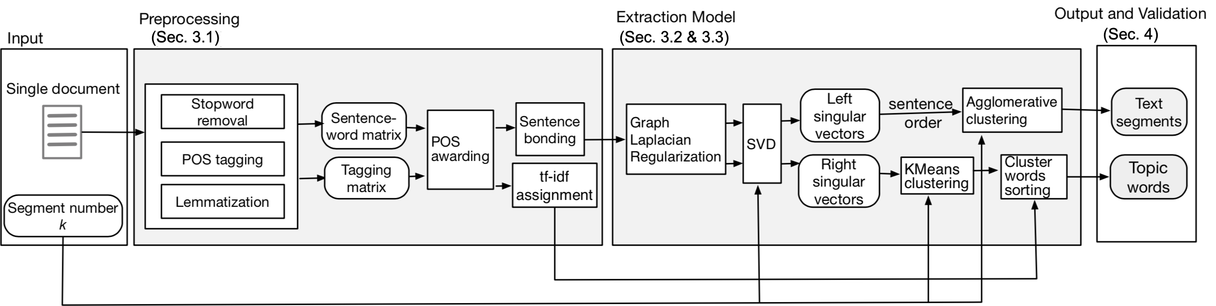
Figure 1. Block diagram summary of the modules comprising BATS, the spectral biclustering methodology we develop in this paper for single-document topic modeling and text segmentation.

1.4. Summary of Contributions

Our key contributions are summarized as follows:

• We develop a novel methodology called BATS that performs topic modeling and text segmentation on a single document simultaneously. BATS is unsupervised and scalable in its implementation, as it does not rely on pre-trained word embedding models.

• We connect the joint topic extraction and segmentation problem to spectral biclustering of sentence-word matrices, and show how a factorization of the graph Laplacian with appropriate pre-processing and post-clustering can lead to effective topic modeling and text segmentation.

• Our evaluation on several datasets establishes that BATS achieves the best combination of topic modeling, text segmentation, and runtime metrics when compared with baselines on single documents. It also verifies the contribution of different components of BATS.

2. Related Work

We identify three areas of related work: biclustering techniques, topic modeling, and text segmentation algorithms.

2.1. Biclustering Techniques

Biclustering techniques (e.g., (Dhillon, 2001; Dhillon et al., 2003; Rohe et al., 2012)) have been proposed to model interactions among two types of nodes represented in a bipartite graph, with nodes of each type grouped into clusters according to different methods. These techniques are widely used in part because of their sound theoretical properties (Dhillon et al., 2003). In (Dhillon, 2001) and (Kluger et al., 2003), the authors propose algorithms which translate input data into bipartite graphs and apply spectral techniques to the adjacency matrices; in (Dhillon, 2001), a block diagonal structure is assumed, while in (Kluger et al., 2003), the case of a checkerboard pattern is considered, with implications to the spectral decomposition. (Rohe et al., 2012) can be viewed as an extension of the algorithm in (Dhillon, 2001) to deal with asymmetric data matrices. By contrast, (Dhillon et al., 2003) proposes a probabilistic approach to graph biclustering, where the input data matrix is treated as a joint probability distribution between two random variables, which are then clustered according to relative entropy and mutual information metrics. Our work builds off the spectral clustering foundations in (Dhillon, 2001; Rohe et al., 2012), accommodating rectangular sentence-word data matrices instead of traditionally assumed square matrices.

2.2. Topic Modeling

Several models have been proposed to extract topics from a corpus consisting of multiple long documents, including Latent Semantic Analysis (LSA) (Deerwester et al., 1990), Non-negative Matrix Factorization (NMF) (Pauca et al., 2004), Probabilistic Latent Semantic Analysis (pLSA) (Hofmann, 2017), Latent Dirichlet Allocation (LDA) (Blei et al., 2003), and variants on LDA, e.g., hierachical modeling (Teh et al., 2005) (see (Daud et al., 2010) for a survey). Recent work has incorporated word and document embeddings jointly to capture “topic vectors” (Angelov, 2020); however, even when these approaches use large pre-trained embedding models, they require corpora on the order of thousands of documents to achieve competitive results, making them unsuitable to applications where data is limited. Analysis on short texts usually faces the issue of sparsity in word occurrences. To overcome this challenge, works such as (Yin and Wang, 2014; Yan et al., 2013) make additional assumptions on word co-occurrence patterns; (Shi et al., 2018; Nguyen et al., 2015; Zhao et al., 2017; Qiang et al., 2017) have resorted to word embeddings which leverage pre-trained models; (Cui et al., 2019; Gao et al., 2017) depend on further external knowledge including social relationships in microblogs and user preferences. One of these, Semantics-assisted NMF (SeaNMF) (Shi et al., 2018), is a variant of NMF designed to handle short documents by learning semantic relationships between words in the corpus. It has been found to outperform other standard techniques such as NMF and LDA (Shi et al., 2018).

Different from these methods, ours aims at identifying topics in a single, newly created document without an extensive training component. To overcome issues of input data sparsity and noise, BATS turns to word-ordering information between sentences and regularization in the spectral clustering phase, as opposed to making additional assumptions on word co-occurrence patterns. Through evaluation on several datasets, we show that BATS outperforms many of the above models on single document topic modeling in terms of topic coherence, topic diversity, and scalability metrics. In particular, compared to the state-of-the-art SeaNMF method, we will see through our experiments that BATS achieves better performance on topic coherence in most cases, and smaller/more scalable runtimes, which is important in the “new and single document” setting we consider in this paper.

2.3. Text Segmentation

Text segmentation algorithms are designed to detect breakpoints in a document and split the document into multiple segments accordingly. Algorithms such as Lexical Chains (Manabu and Takeo, 1994) and TextTiling (Hearst, 1997) use lexical co-occurrence and distribution patterns to divide sets of paragraphs into multi-paragraph sub-blocks that become segments. A potential drawback of these approaches, however, is that the segments are not associated or labeled with explicit topic information, and that it is not always clear how to translate from a lexical distribution to topics. This motivates the consideration of topic modeling and text segmentation jointly.

More recently, to improve segmentation performance, topic-based segmentation methods such as TopSeg (Brants et al., 2002), LDA_MDP (Misra et al., 2011), and TopicTiling (Riedl and Biemann, 2012) have been proposed. Similar to the topic modeling algorithms discussed above, these segmentation methods depend heavily on the training process, and usually require training on a large corpus (Chang et al., 2009). This is problematic when only small datasets are available, let alone in the single document case that we consider in this paper. Through biclustering of the sentence-word matrix and development of other pre-processing techniques, BATS does not demand an expensive training process. Other recent approaches, such as SupervisedSeg (Koshorek et al., 2018) and SegBot (Li et al., 2018), have modeled the task as a supervised learning problem and employed deep recurrent networks while others rely on massive language representation models such as Bidirectional Encoder Representations from Transformers (BERT) (Devlin et al., 2018). Generally, these models are pre-trained on large historical datasets and can be used in an application with little to no fine-tuning required. However, loading such models may use substantial computational resources and their reliance on historical data can introduce biases and gaps. By contrast, BATS is designed to be computationally efficient and flexible enough to accurately handle novel text. We find that BATS obtains an order of magnitude smaller runtime compared with BERT applied to text segmentation, which is important in our “new and single document” setting. Further, our evaluation shows that BATS outperforms the segmentation methods discussed here on single documents across several datasets.

3. Spectral Biclustering Methodology

As shown in Figure 1, our proposed methodology BATS consists of two main stages: the text preprocessing stage (Section 3.1) and the extraction stage, with the latter broken down into graph Laplacian regularization (Section 3.2), singular vector extraction (Section 3.3), and sentence/word clustering (Section 3.4). Topics and segments emerge from the word and sentence clusters, respectively. In this section, we detail the development of these modules, and discuss how they address the issue of sparsity associated with modeling a single document.

3.1. Document Preprocessing and Matrix Construction

Consider an input document comprised of $m$ sentences, indexed $i=1,...,m$. We denote $\mathcal{W}=\{w_{1},...,w_{n}\}$ as the set of words we are interested in for modeling, indexed $j=1,...,n$. In defining $\mathcal{W}$, we do not include all the words that ever appear in the document; instead, a word is included in $\mathcal{W}$ if and only if it appears in more than one sentence in the document and it is not in a stopword list. In this way, $\mathcal{W}$ excludes “degree-one” words that can skew models in single documents; we observe that these words often behave as pure noise in our inference algorithms.

Let $X=[X_{ij}]\in\mathbb{R}^{m\times n}$ denote the sentence-word matrix. Even after excluding degree-one words, we still expect this matrix will be sparse, with a significant number of $X_{ij}=0$. We develop two steps to construct $X$, taking into account both word order and parts-of-speech information:

3.1.1. Step 1. Using parts-of-speech information

Our first optimization trick is based on parts-of-speech (POS) tags, which are generated through analysis of the word positions in the sentences (Goldberg and Nivre, 2012). In particular, the lexical model presented in (Elman, 1990) shows hierarchies exist according to syntactic/semantic similarities of words; looking into them, it is clear that nouns and verbs convey more information than other word types, and thus should be given a larger weight (Resnik, 1993). As a result, letting $X^{o}=[X^{o}_{ij}]$ where $X^{o}_{ij}$ is the number of occurrences of word $w_{j}\in\mathcal{W}$ in sentence $i$, we define

(1) $$X^{a}=X^{o}+\lambda T,$$

where $T=[T_{ij}]$, $T_{ij}=1$ if $X^{o}_{ij}\neq 0$ and $w_{j}$ is tagged as a noun or verb in sentence $i$, and $T_{ij}=0$ otherwise. $\lambda>0$ is a scalar parameter for awarding POS; by default, $\lambda=1$. In our implementation, Python’s spaCy module is used to tag the words, as this pre-trained model based on word positions is more robust to novel words or topics than would be, for instance, a word-embedding model.

3.1.2. Step 2. Transformation by using word-order information

Our incorporation of word-order information is based on the intuition that words in neighboring sentences are likely to be similar in their constituent topics, with this effect decaying as the sentences grow further apart. Assumptions on words appearing within a certain window being related can be found in other text analysis techniques as well, including word embedding models (Pennington et al., 2014). Concretely, we bond neighboring sentences to the current sentence according to

(2) $$X_{i}=\sum^{i+w}_{\ell=i-w}d^{|\ell-i|}X_{\ell}^{a},\qquad i=1,...,m,$$

where $X_{i}=(X_{i1},...,X_{in})$ is the $i$th row of $X$ and $X_{\ell}^{a}$ is the $\ell$th row of $X^{a}$ for $\ell=1,...,m$ (for $\ell<1$ and $\ell>m$, $X^{a}_{\ell}$ is taken as a vector of zeros). Parameter $w$ controls the size of the bonding window, and $d\in[0,1]$ is a decay rate for the distance. In this way, the presence of a word in one sentence will impact neighboring sentences, and words appearing in several consecutive sentences are increased in importance. Doing so also alleviates the issue of sparsity associated with modeling single documents, as each sentence’s data smoothens its neighbors’ representations too. The procedure for determining the values of $w$ and $d$ will be discussed in Section 3.2.

3.2. Graph Laplacian and Regularization

3.2.1. Intuition

Consider the bipartite graph $\mathcal{G}(X)$ of the sentence-word matrix $X$, where the sentences $i=1,...,m$ and words $j=1,...,n$ each form a node set, and edge $(i,j)$ of weight $X_{i,j}$ is in $\mathcal{G}(X)$ if and only if $X_{i,j}\neq 0$. Intuitively, this graphical representation will capture some relatedness information between words and sentences, e.g., words that frequently occur together, and are therefore likely to be part of the same topic, should have a high number of short paths to each other. This bipartite graph is likely to have nodes whose degrees follow a power law distribution, both as a product of Zipf’s Law for word frequency distributions (Zipf, 1949, 1953) and because empirically real world networks often exhibit power laws (Eikmeier and Gleich, 2017). The graph Laplacian is known to be a useful matrix representation for clustering graphs with heterogeneous node degrees given the relationship between its spectral properties and the connected components of the graph (Von Luxburg, 2007). To further address the sparsity issue, we will develop a regularized version of the Laplacian, as it has been shown to improve the performance of spectral clustering algorithms on sparse matrices (Amini et al., 2013; Chaudhuri et al., 2012; Qin and Rohe, 2013).

3.2.2. Constructing the Laplacian

Formally, define two diagonal matrices $P=\mbox{diag}(P_{1},...,P_{n})\in\mathbb{R}^{n\times n}$ and $O=\mbox{diag}(O_{1},...,O_{m})\in\mathbb{R}^{m\times m}$ where $P_{j}=\sum_{i=1}^{m}X_{ij},j=1,...,n$ and $O_{i}=\sum_{j=1}^{n}X_{ij},i=1,...,m$ are the row and column sums of $X$. With regularization parameters $\tau_{p},\tau_{o}\geq 0$, the regularized graph Laplacian $L\in\mathbb{R}^{m\times n}$ is computed according to

(3) $$P_{\tau}=P+\tau_{p}I_{p},\qquad O_{\tau}=O+\tau_{o}I_{o},\qquad L=(O_{\tau})^{-\frac{1}{2}}X(P_{\tau})^{-\frac{1}{2}},$$

where $I_{p}$ and $I_{o}$ are identity matrices. Multiplying these by regularization parameters $\tau_{p}$ and $\tau_{o}$ can resolve issues due to poor concentration since the degrees for every vertex are inflated. Following prior work (Qin and Rohe, 2013) which has indicated that such regularization parameters should be proportional to the average degrees of the vertices (so that the asymptotic bounds will be indicative of the mis-clustering rate), we set the average degrees as defaults, i.e., $\tau_{p}=\sum_{j}P_{j}/n$ and $\tau_{o}=\sum_{i}O_{i}/m$.

Algorithm 1 Matrix decomposition on regularized Laplacian.

1:INPUT: Original sentence-word matrix $X^{o}$, POS-based matrix $T$

2:PARAMETER: Awarding value $\lambda$, window size $w$, decaying rate $d$, segment number $k$

3:OUTPUT: Matrix $U$ for sentences and $V^{T}$ for words

4:function MAT_DECOMP($X^{o}$, $w$, $d$)

5:    if $\lambda>0$ then

6:         $X^{a}=X^{o}+\lambda T$   //Word awarding

7:    else

8:         $X^{a}=X^{o}$     

9:    $F\leftarrow$ tf-idf($X^{a}$)   //Tf-idf assignment

10:    for $i\leftarrow 1,...,n$ do

11:         $X_{i}=\sum^{i+w}_{\ell=i-w}d^{|\ell-i|}X_{\ell}^{a}$   //Sentence bonding     

12:    for $j\leftarrow 1,...,n$ do

13:         $P_{j}\leftarrow\sum_{i=1}^{m}X_{ij}$     

14:    for $i\leftarrow 1,...,m$ do

15:         $O_{i}\leftarrow\sum_{j=1}^{n}X_{ij}$     

16:    $\tau_{p}\leftarrow\sum_{j}P_{j}/n$, $P_{\tau}\leftarrow P+\tau_{p}I_{p}$   //Regularization

17:    $\tau_{o}\leftarrow\sum_{i}O_{i}/m$, $O_{\tau}\leftarrow O+\tau_{o}I_{o}$  //Regularization

18:    $L=(O_{\tau})^{-\frac{1}{2}}X(P_{\tau})^{-\frac{1}{2}}$   //Graph Laplacian

19:    $U\Sigma V^{T}=L$   //Singular value decomposition

20:    for $u^{\prime}\leftarrow$ rows of $U$ do

21:         $u^{\prime}\leftarrow u^{\prime}[1:k]$   //Reserve first $k$ dimensions

22:         $u^{\prime}\leftarrow u^{\prime}/\sqrt{\sum_{i}u_{i}^{{}^{\prime}2}}$   //L2 normalization on $U^{\prime}$     

23:    for $v^{\prime}\leftarrow$ rows of $V$ do

24:         $v^{\prime}\leftarrow v^{\prime}[1:k]$   //Reserve first $k$ dimensions

25:         $v^{\prime}\leftarrow v^{\prime}/\sqrt{\sum_{i}v_{i}^{{}^{\prime}2}}$   //L2 normalization on $V^{\prime}$     

26:    return $U^{\prime}$, $V^{\prime}$, $F$  //$U^{\prime}$ for sentences, $V^{\prime}$ for words

3.3. Sentence and Word Singluar Vectors

3.3.1. Intuition

Our main observation is that sentence-word interactions in a document may be modeled by a stochastic co-block model (SCBM) (Karrer and Newman, 2011; Qin and Rohe, 2013), whose structure can be inferred through spectral clustering. SCBM is a bipartite graph generalization of the standard block model (Rohe et al., 2012), where there are $k_{1}$ blocks of nodes on the left side of the graph and $k_{2}$ blocks of nodes on the right. The interactions between nodes at two sides are governed by a matrix $B\in\mathbb{R}^{k_{1}\times k_{2}}$, i.e., for any $u$ in the $i$-th left block and $v$ in the $j$-th right block, $\Pr[\{u,v\}\in E]=B_{i,j}$. In our setting, each right node corresponds to a word, and words in the same block can be interpreted as in the same topic. Each node to the left corresponds to a sentence, and sentences in the same block corresponds to the same segment. A word is connected to a sentence if it appears in the sentence at least once.

Spectral clustering can be used to recover the block structure in an SCBM. This algorithm first finds the leading singular vectors and values of the bipartite graph’s adjacency matrix, and then runs standard clustering algorithms (e.g., k-means) on the leading singular vectors/values. The algorithm is known to be effective for sparse SCBM because it can effectively remove singular vectors along directions that contain stronger noise than signal. A synthetic example of this is shown in Fig. 2, where we have generated 2000 sentences and 5000 words according to an SCBM with four blocks each. The dataset is too sparse for standard degree-based algorithms, such as counting shared neighbors (Jarvis and Patrick, 1973) or using Jaccard similarity (Niwattanakul et al., 2013), to recover these blocks (Fig. 2b). Nevertheless, we notice that all the singular vectors/values beyond the first three correspond to noise (Fig.  2a). Therefore, when we perform clustering only on the leading dimensions of the singular vectors, we are able to exactly recover the blocks (Fig. 2c). This motivates us using the singular vectors to cluster words and sentences.

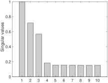
(a) Top-10 singular values of the sentence-word matrix.

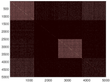
(b) Heatmap of pairwise distances between words.

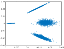
(c) Right singular vectors plotted in the first two dimensions.

Figure 2. Synthetic example illustrating the use of spectral decomposition to recover the block structure in a sentence-word matrix generated according to an SCBM with four blocks of sentences and words.

3.3.2. Obtaining a low dimensional embedding

We consider the singular value decomposition (SVD) of the graph Laplacian $L$. By definition, the SVD yields

(4) $$L=U\Sigma V^{T},$$

where $U\in\mathbb{R}^{m\times m}$ and $V\in\mathbb{R}^{n\times n}$ are unitary matrices and $\Sigma$ contains the singular values $\sigma_{1},...,\sigma_{\max\{m,n\}}$ on its diagonal. Since $L^{T}L=V(\Sigma^{T}\Sigma)V^{T}$ is a measure of similarity between words, counting their degrees of connectivity via sentences, and $LL^{T}=U(\Sigma\Sigma^{T})U^{T}$ is a measure of similarity between sentences, counting their degree of connectivity via words, the SVD can be used to cluster words (using $V$) and sentences (using $U$). Further, as the eigenvalues of $L^{T}L$ and $LL^{T}$ are the square of the singular values in $\Sigma$, we introduce another parameter $k$ which denotes the number of left $U_{1},...,U_{k}\in\mathbb{R}^{m}$ and right $V_{1},...,V_{k}\in\mathbb{R}^{n}$ dominant singular vectors used, where we assume the singular values are in decreasing order $\sigma_{1}\geq\sigma_{2}\geq\cdots$. We then re-normalize the rows of the resulting matrices

(5) $$V^{\prime}=[V^{\prime}_{i\ell}]=[V^{\prime}_{1}\;V^{\prime}_{2}\;\cdots\;V^{\prime}_{k}],\quad U^{\prime}=[U^{\prime}_{j\ell}]=[U^{\prime}_{1}\;U^{\prime}_{2}\;\cdots\;U^{\prime}_{k}]$$

to have unit length, i.e., so that $\sum_{\ell}V_{i\ell}^{{}^{\prime}2}=\sum_{\ell}U_{j\ell}^{{}^{\prime}2}=1$ for each sentence $i$ and word $j$. Following (Von Luxburg, 2007), which suggests that the dimensionality should be consistent with the number of clusters to be grouped, we use the same parameter $k$ for both $U$ and $V$.

The full decomposition process developed in Sections 3.1-3.3 is summarized in Algorithm 1.

3.3.3. Impact of $w$ and $d$

Recall the window $w$ and decay $d$ parameters from (2). We investigate the impact of these parameters on the matrix decomposition in (5) by considering the L2-norm distances between the resulting sentence vectors in $U$. Figure 3 gives heatmaps of these distances for two arbitrary documents in one of our datasets (see Section 4.1). Since neighboring sentences should cover similar topics, we seek values of $w$ and $d$ for which ordering information is clearly embedded in the matrix. In Figure 3(a), for small values of $w$ (i.e., $w=0,1$), the sentence order is less clear as the elements near the diagonal are more blurry. As $w$ increases, the pattern becomes more obvious, and when $w=3$ we observe clear block patterns in the heatmap. When $w$ is increased further (i.e., to $w=5$), the sharpness of the block pattern does not continue to improve; intuitively, sentences at the far ends of the bonding window for large $w$ will have higher dissimilarity, but this effect is blunted by the decay $d$ (which is $0.7$ here). Since a higher $w$ also increases the runtime of the method, in considering several documents, we find that the best choice of $w$ is typically between $3$ and $5$ (i.e., the number of topic-neighboring sentences is $6$ to $10$).

Figure 3. Heatmaps of the pairwise distances between sentence vectors in the SVD for two random sampled document taken from the Introductions dataset under different values of parameters $w$ and $d$. (a) varies $w$ for fixed $d=0.7$ and varies $d$ for fixed $w=3$ on the first randomly sampled document. (b) varies $w$ for fixed $d=0.7$ and varies $d$ for fixed $w=3$ on the second randomly sampled document.

By this logic, then, the value of $d$ should be significantly lower than $1$. As it is decreased in Figure 3(b) (i.e., from $d=0.9$), we see that the sharpness of the blocks improves, with $d=0.7$ giving the clearest pattern. Beyond this (i.e, $d=0.5,0.3$), however, the sharpness begins to decrease. In these cases, neighboring sentences are assigned lower weights, confirming that the SVD uncovers topic similarity between neighbors. In considering several documents, we find that the best choice is $d\approx 0.7$ for this reason. In Section 4, we will verify that $w=5,d=0.7$ leads to the highest average performance on the topic modeling and text segmentation metrics for all datasets considered.

3.4. Word and Sentence Clustering

With the embedding from (5) in hand, we move to obtain topics and segments via spectral clustering of the word $V$ and sentence $U$ matrices respectively. Following (Von Luxburg, 2007), we consider the problem from a graph cut point of view, where the cuts are taken on a similarity graph of words or sentences.

Formally, let $G=[g_{i,j}]\in\mathbb{R}^{n\times n}$ be the similarity matrix among a set of $n$ nodes $v_{1},...,v_{n}$ (i.e., words or sentences), where $g_{i,j}\geq 0$ is the similarity between nodes $v_{i}$ and $v_{j}$. We seek to minimize $KCut(S_{1},...,S_{k})=\frac{1}{2}\sum_{p=1}^{k}cut(S_{p},\bar{S_{p}})$ while $cut(S_{p},\bar{S_{p}})=\sum_{\begin{subarray}{c}i\in S_{p},j\in\bar{S_{p}}\end{subarray}}g_{i,j}$. Note $S=\{S_{1},S_{2},...,S_{k}\}$ is a grouping of the nodes into $k$ disjoint sets $S_{1},...,S_{k}$. A simple and straightforward solution for this minimization problem is to cut off individual nodes which are weakly connected to the rest. However, there is usually no topic with one word or text segment with one sentence, therefore, the groups of words or sentences are supposed to have more balanced sizes. As a result, the objective function needs to take group sizes into consideration and build the balanced cut problem

(6) $$BCut(S_{1},...,S_{k})=\sum_{p=1}^{k}\frac{cut(S_{p},\bar{S_{p}})}{|S_{p}|}.$$

Taking group sizes into account makes the problem NP hard and requires further relaxation. We reorganise the problem by defining a group indication matrix $H=[h_{1}\cdots h_{k}]\in\mathbb{R}^{n\times k}$ consisting of $k$ weighted indicator vectors $h_{p}=(h_{1,p},...,h_{n,p})^{T},p=1,...,k$ where

(7) $$h_{i,p}=\begin{cases}1/\sqrt{|S_{p}|}&\text{if node $v_{i}\in S_{p}$}\\ 0&\text{otherwise.}\end{cases}$$

We can see $H^{T}H=I$ where $I$ is the identity. Letting $G$ be the node similarity graph, we define its degree matrix as $D=\mbox{diag}(d_{1},...,d_{n})$ where $d_{i}=\sum_{j}g_{ij},i=1,...,n$, and the unnormalized graph Laplacian as $L_{u}=D-G$. Through some easy math, we can get

(8) $$h_{p}^{T}L_{u}h_{p}=\frac{cut(S_{p},\bar{S_{p}})}{|S_{p}|},\text{ for }p=1,...,k.\vspace{-1mm}$$

Combining this with (6), we conclude that

(9) $$\vspace{-1mm}BCut(S_{1},...,S_{k})=\sum_{p=1}^{k}h_{p}^{T}L_{u}h_{p}=Tr(H^{T}L_{u}H).\vspace{-1mm}$$

Thus, the minimization problem can be presented as

(10) $$\begin{split}\min_{\begin{subarray}{c}S_{1},\cdots,S_{k}\end{subarray}}Tr(H^{T}L_{u}H)\text{ subject to $H^{T}H=I$, $H$ defined as (\ref{eq_H})}.\end{split}$$

This problem is equivalent to minimizing (6) and is NP-hard. Therefore, in the BATS methodology, we relax this constraint by allowing $h_{i,p}\in\mathbb{R}$ to take any arbitrary value, and turn (10) into

(11) $$\min_{\begin{subarray}{c}H\in\mathbb{R}^{n\times k}\end{subarray}}Tr(H^{T}LH)\text{ subject to }H^{T}H=I.\vspace{-1mm}$$

This approach allows us to employ clustering algorithms to solve the minimization problem. In the following sections, we detail our methods for solving (11) to cluster words (Section 3.4.1) and sentences (Section 3.4.2), respectively.

3.4.1. Topics via word clustering

To obtain the topics, we consider spectral clustering for the normalized word matrix $V^{\prime}$ in (5). Since each row $v^{\prime}_{j}\in\mathbb{R}^{k},j=1,...,n$ of $V$ is a $k$-dimensional representation of a word, the clustering optimization in (9) takes these $n$ words as the nodes to be grouped into $k$ sets $S_{1},S_{2},...,S_{k}$ based on the similarities $g_{j,j^{\prime}}$ between pairs of word representation vectors $v_{j}$ and $v_{j^{\prime}}$. This is equivalent to minimizing the pairwise deviations between representations of nodes within the sets:

(12) $$S=\underset{\{S_{1},...,S_{k}\}}{\arg\min}\sum_{p=1}^{k}\frac{\sum_{j,j^{\prime}\in S_{p}}||v^{\prime}_{j}-v^{\prime}_{j^{\prime}}||^{2}}{2|S_{p}|}.$$

This optimization is equivalent to a KMeans clustering (Lloyd, 1982) of the vectors $v^{\prime}_{1},...,v^{\prime}_{n}$. The number of clusters is determined by the number of segments $k$, and each resulting word cluster $S_{p}$ refers to a topic. To obtain a description of each topic in terms of its top words, we further rank the words in each cluster according to the standard term frequency-inverse document frequency (tf-idf) metric (Rajaraman and Ullman, 2011) applied to the awarded sentence-word matrix $X^{a}$ in (1). The tf-idf assignment matrix $F$ is obtained during the matrix decomposition process and it is the same size of $X^{a}$. To assign each word a single tf-idf score for sorting, we sum the tf-idf scores of each word over all sentences.

3.4.2. Segments via sentence clustering

We then turn to clustering the normalized sentence matrix $U^{\prime}$ in (5) to obtain the segments. Compared with the topic clustering problem, this one will have more constraints since the clusters are related to the sentence orders and the cluster sizes can be uneven. As a result, the KMeans method is no longer applicable, and we resort instead to an agglomerative clustering method with connectivity constraints (Davidson and Ravi, 2005) to solve (9). In agglomerative clustering, nodes are grouped together sequentially according to pairwise similarities: the process recursively merges two groups of nodes that yield the minimum between-cluster distance.

Formally, recall that the sentence embeddings are the rows $u^{\prime}_{i}\in\mathbb{R}^{k},i=1,...,m$ of the matrix $U^{\prime}$. We form the graph of sentences $G_{S}=(V,E_{S})$, where $V=\{i|i=1,2,...,m\}$ and $E_{S}=\{(i,j)|i,j=1,2,...,m,i\neq j\}$, with the weight of the edge $(i,j)\in E_{S}$ being the cosine similarity between $u^{\prime}_{i}$ and $u^{\prime}_{j}$. The ordering constraint should be such that only adjacent sentences can be clustered; we therefore initialize a connectivity graph $G_{C}^{1}=(V,E_{C}^{1})$ where for all pairs of nodes $i,j\in V$, $(i,j)\in E_{C}^{1}$ if and only if $j=i+1$, i.e., each node connects to the next sentence. Letting $S_{i}^{r}$ denote cluster $i$ of the sentences at the $r$th iteration, initialized as $S_{i}^{1}=\{i\}$ for each $i$, the merging operation of our constrained agglomerative clustering is given by

(13) $$(S_{p}^{r},S_{q}^{r})=\underset{(i,j)\in E_{C}^{r}}{\arg\min}\;\overline{D}(S_{i}^{r},S_{j}^{r}),\quad S_{p}^{r+1}=S_{p}^{r}\cup S_{q}^{r},\quad S_{q}^{r+1}=\emptyset,\quad E_{C}^{r+1}=E_{C}^{r}\setminus\{(p,q)\}\cup\{(p,a^{r}(q)\},$$

for $r=1,...,m-k$, where $\overline{D}(S_{i}^{r},S_{j}^{r})$ refers to the distance between the sets $S_{i}^{r}$ and $S_{j}^{r}$, which is treated as the average distance between sentences in $S_{i}^{r}$ and $S_{j}^{r}$ according to their link weights in $E_{S}$, and $a^{r}(q)$ is the single node that $q$ points to in $G_{C}^{r}$. In each iteration, the two adjacent clusters of sentences that have minimum distance are merged together. The procedure ends after $r=m-k$ iterations, when there are $k$ clusters $i$ for which $S_{i}^{k}\neq\emptyset$; these are taken as the segments.

3.4.3. Advantages of joint topic modeling and text segmentation

In the BATS methodology, segmentations are produced from sentence clusters whereas topics are produced from word clusters. A key observation we have made in the design of BATS is that we can indeed use one simple bi-clustering algorithm to simultaneously identify sentence and word clusters, based on two simple assumptions: (i) when two sentences are in the same cluster (segment), the same set of words are more likely to appear in both sentences, and (ii) when two words are in the same cluster (topic), these words are more likely to co-appear in the same sentences.

Algorithm 2 BATS topic modeling and text segmentation.

1:INPUT: Single text document, segment number $k$

2:PARAMETER: Awarding value $\lambda$, window size $w$, decaying rate $d$

3:OUTPUT: Topic words, text segments

4:procedure MainProcess(text, $k$, $\lambda$, $w$, $d$)

5:    Remove degree-one words from text.

6:    Compute sentence-word matrix $X^{o}$ and POS-based matrix $T$.

7:    $U^{\prime},V^{\prime},F\leftarrow$ MAT_DECOMP($X^{o}$, $T$, $\lambda$, $w$, $d$, $k$). // Alg.1

8:    

Cluster the rows of $V^{\prime}$ with KMeans into $k$ clusters. Sort the words in each cluster by $F$ (tf-idf scores).

9:    

Cluster the rows of $U^{\prime}$ with agglomerative clustering into $k$ clusters with a connectivity constraint.

10:    Topic words $\leftarrow$ Sorted words in each cluster

11:    Text segments $\leftarrow$ Sentence clusters

12:    return Topic words, Text segments

In other words, the segmentation and topic modeling tasks are coupled through the bi-clustering algorithm in BATS, which uses sentence-word interactions to identify a joint latent structure for segments and topics. The model of which sentences are contained in which segments simplifies the process of identifying topics, and vice versa. Let us consider a concrete example, in which a document consists of 10 sentences. Each sentence may have different topic distributions, e.g., sentence 1 has 80% of words from a “science” topic and 20% from a “health” topic, whereas sentence 7 has 40% from the “science” topic and 60% from the “health” topic. If we assume that words from the same segment come from the same topic distribution, when the ground-truth of the segmentation is known – e.g., segment 1 consists of the first four sentences and segment 2 consists of the last six sentences – we are narrowing the set of topics these words are assumed to be sampled from. Specifically, in this example, we effectively observe two sets of words sampled from two topic distributions (one for each segment), instead of 10 (one for each sentence). This extra information simplifies the process of identifying topics. In fact, the bi-clustering algorithm implicitly uses this information in the singular value decomposition step: it uses sentence clusters (segments) to improve word clusters, and vice versa. Therefore, we expect that doing topic modeling and text segmentation jointly will improve the quality of both tasks, with the added advantage of being more computationally efficient than doing both separately.

3.5. BATS Methodology Summary

The full BATS topic modeling and text segmentation methodology (including Algorithm 1) developed throughout this section is summarized in Algorithm 2. The inputs are the single text document of interest and $k$, the number of topics and segments to extract. The algorithm begins with denoising, which removes all degree-one words, and constructing the sentence-word matrix $X^{o}$ and parts-of-speech matrix $T$. $X^{o}$ and $T$ are then inputted to the matrix decomposition procedure, detailed in Algorithm 1, which employs sentence bonding and graph Laplacian regularization to obtain the matrices $U^{\prime}$ and $V^{\prime}$, containing the encodings of the sentences and words, and the tf-idf matrix $F$. The rows of $V^{\prime}$ are then clustered into $k$ clusters of words via KMeans, with the words in each cluster sorted by tf-idf score in $F$, forming the topics. Finally, the rows of $U^{\prime}$ are clustered into $k$ clusters of sentences via constrained agglomerative clustering, forming the segments.

3.6. Time Complexity Analysis

Recall from Section 1.1 that an important setting for the “single and new document” setting is in the presence of constrained computational resources. Thus, we also perform a complexity analysis to investigate the efficiency of our algorithm, given the importance of low runtimes.

From Algorithm 1, note that there are three main procedures in BATS which have major impacts on the time complexity: matrix decomposition, KMeans clustering for words, and agglomerative clustering for sentences. The matrix decomposition process consists of multiple matrix multiplication and summation operations, of which matrix multiplication dominates with a complexity of $O(\max(m^{3},n^{3}))$, where $m$ and $n$ are the number of sentences and words, respectively. However, in our application, the sentence-word matrix is sparse and therefore enables some optimizations in the matrix decomposition procedure. Specifically, iterative methods such as primme (Stathopoulos and McCombs, 2010) can decompose sparse matrices with a time complexity of $O(mnr)$, where $r$ is the number of singular vectors. Formally, we can show that when the number of singular vectors is small, the time complexity is described as follows:

Lemma 0.

For a given document, assume $m$ and $n$ are the number of sentences and words, respectively. If the number of non-zero singular values of the sentence-word matrix $X^{a}$ is sufficiently small, then the runtime of BATS on the document can be approximated as $O(mnr+n)$.

Proof.

In the KMeans clustering procedure, all $n$ word vectors are compared to $k$ centroids to find the closest centroid, and this step iterates $t_{K}$ times, leading to the time complexity of $O(nt_{K}k)$. In the constrained agglomerative procedure, the similarities between $m$ sentence vectors are computed for clustering, and with $t_{A}$ iterations, the time complexity is $O(t_{A}m\log m)$ with the efficient priority queue implementation (Manning et al., 2008). For the matrix decomposition, as discussed above, using an iterative method such as primme leads to a time complexity of $O(mnr)$. The overall time complexity of our method is the sum of all these procedures, which leads to

(14) $$O\left(mnr+nt_{K}k+t_{A}m\log m\right).\vspace{-2mm}$$

Since $O(mnr)\gg O(m\log m)$, $k\ll n$, and $r\ll m$ by assumption of a low-rank sentence-word matrix, this complexity can be approximated as $O(mnr+n)$. ∎

Thus, BATS has a much lower time complexity than $O(\max(n^{3},m^{3}))$, with the difference being particularly pronnounced when $n\gg m$. The scalability and small runtimes of BATS will be verified experimentally in Section 4.4.

4. Experimental Evaluation and Discussion

We turn now to evaluating our BATS methodology. After describing the datasets (Section 4.1), we consider performance against baselines on the topic modeling (Section 4.2) and text segmentation (Section 4.3) tasks. Then, we consider the scalability of our method (Section 4.4). Finally, we conduct an ablation study to determine the impact of various components of BATS (Section 4.5).

4.1. Description of Datasets

We consider documents from six datasets – Textbook, Lectures, Introductions, Choi, Wiki, and News – obtained from different text applications. Basic statistics on these datasets are given in Table 1, including the number of documents, the average sentences per document, the average word counts per document, and the average sparsity per document (fraction of zero entries in the $X^{a}$ matrix), both before and after the preprocessing procedures described in Section 3.1. More specifics on these datasets are as follows:

(i) Textbook dataset: This is drawn from the medical textbook in (Walker et al., 1990). Each chapter is treated as a document, and each section as a segment. The numbers of segments per document and sentences per segment have high variance. Moreover, segments within a document tend to be similar in their constituent words, as they are different sections of the same chapter. As a result, this dataset helps us test on cases where documents have different segments discussing similar topics.

Table 1. Basic statistics of the six datasets used for evaluation.

Dataset	Documents	Avg. sentences	Avg. segments	Avg. words	Avg. words	Avg distinct words	Avg. distinct words	Avg. sparsity	Avg. sparsity
		per doc	per doc	before preproc.	after preproc.	before preproc.	after preproc.	before preproc.	after preproc.
Textbook	227	136	4	3551	2590	640	241	97.9%	75.2%
Lectures	55	392	8	8002	4924	686	342	99.0%	89.0%
Introductions	2135	195	5	7022	4752	1016	449	98.6%	84.8%
Choi	920	74	10 (const)	1673	1489	650	162	98.0%	76.5%
Wiki	727,000	60	4	1154	1007	521	334	$96.3\%$	$89.6\%$
News	300,000	51	4	1096	730	516	321	$97.1\%$	$87.2\%$

(ii) Lectures dataset: This dataset contains transcripts of conversational lectures on AI and physics topics (Eisenstein and Barzilay, 2008). As each lecture is divided into sections, we treat lectures as documents and sections as segments. Each lecture script has 6-10 sections. Compared with the other datasets, the sentences are more conversational, tending to be shorter and simpler. Therefore, this dataset helps us examine algorithm performance on lengthy conversational documents.

(iii) Introductions dataset: In this dataset, every document is an artificial combination of abstracts and introductions from academic articles in different fields (Chambers., 2013). We randomly choose 3-8 articles, extract the abstract and introduction as one sample, and combine multiple samples into one document. Each sample is treated as one segment. Compared with the other datasets, this will allow us to test on cases with large segment sizes, uneven segment lengths, and a diverse set of topics.

(iv) Choi dataset: This is a standard dataset (Choi, 2000) widely used to evaluate text segmentation approaches. The documents in the dataset are artificial combinations of the first $\ell$ sentences of the documents in the Brown corpus (Francis and Kucera, 1979). Each document has 10 segments, with few sentences per segment. Because the dataset lacks explicit topic distributions and contains mostly segments that are too short for topic modeling, we use it only for evaluating text segmentation.

(v) Wiki dataset: This is the WIKI-727k dataset from (Koshorek et al., 2018) which is comprised of over 727,000 articles from English Wikipedia. Its vocabulary size exceeds 800,000 tokens. We treat articles as documents and, following (Koshorek et al., 2018), use the Punkt Sentence Tokenizer from the nltk library (Bird et al., 2009) to generate ground truth segments. We include this dataset primarily to test the performance of BATS on large corpora, although it also provides a new genre of natural text covering a wide variety of encyclopedia topics.

(vi) News dataset: Finally, we include a news dataset generated by following links shared on Twitter. We use a collection of Tweets from (Li et al., 2017) that focus on news related to the 2016 US presidential election and follow the shared links to scrape text from the linked articles. The news dataset consists of about 300,000 documents with a vocabulary size of over 80,000. Each article is treated as a document and ground truth segments are generated using the Punkt Sentence Tokenizer.

4.2. Topic Modeling

4.2.1. Baselines

We compared BATS against six baselines for topic modeling:

(i) Latent Dirichlet Allocation (LDA) (Blei et al., 2003; Sarne et al., 2019): LDA is a probabilistic topic model which uses two independent Dirichlet priors for the document-topic and word-topic distributions. It trains a model to best estimate the Bayesian probabilities $P(word|topic)$ and $P(topic|document)$. We use the sklearn implementation in Python with the default parameters.

(ii) Hierarchical Dirichlet Process (HDP) (Teh et al., 2005): HDP is a mixed-membership model which extends LDA to an unknown number of topics by building a hierarchy. Specifically, it builds a two-level hierarchical Dirichlet process at the document-level and the word-level to perform parameter inference. We use the gensim implementation in Python with the default parameters.

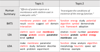
Figure 4. Example of topics extracted from an arbitrary document in the Introductions dataset. Words in color red are those consistent with a human-generated summary, and duplicated words are boldfaced. Our results produce the best descriptions as well as the least overlaps.

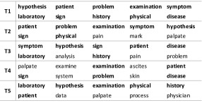
Figure 5. Example of topics extracted from one document (known to have five topics) in the Textbook dataset by LSA. Duplicated words are denoted in boldface. There is high overlap, motivating the need to consider topic diversity in addition to coherence.

(iii) Latent Semantic Analysis (LSA) (Deerwester et al., 1990): LSA decomposes a document-word matrix, based on TF-IDF scores, into a document-topic matrix and a topic-word matrix; the decomposition is performed through a truncated SVD technique. We use the gensim implementation in Python.

(iv) Probabilistic Latent Semantic Analysis (pLSA) (Hofmann, 2017): pLSA is developed from LSA, using a probabilistic method instead of SVD to find the latent topics via generative modeling of the observed document-word matrix. We implement pLSA de-novo in Python, using 30 as the max number of iterations, 10.0 as the breaking threshold, and $k$ as the number of topics.

(v) Non-negative Matrix Factorization (NMF) (Pauca et al., 2004): NMF is a linear-algebraic model which factorizes a high-dimensional matrix into two lower-dimensional ones. In this case, NMF decomposes the document-word matrix (based on TF-IDF scores) into a topic matrix and a coefficient matrix for the topics. We use the sklearn implementation in Python with the default parameters.

(vi) Semantics-assisted Non-negative Matrix Factorization (SeaNMF) (Shi et al., 2018): SeaNMF introduces word-context semantic correlations into NMF to extract topics particularly from short texts. The semantic correlations between the words and their contexts are learned from the Skip-Gram with Negative Sampling (SGNS) word embedding technique (Mikolov et al., 2013a; Mikolov et al., 2013b) to address sparsity. The objective function of SeaNMF preserves both the word-document matrix and semantic correlation matrix. We use the author’s Python implementation available at https://github.com/tshi04/SeaNMF.

Since our focus is on single document topic modeling, we evaluate the models on each document separately. Given that the baselines usually learn across multiple documents, to provide a fair comparison, we treat the sentences within each document as the “documents” for the baselines, i.e., we feed them the preprocessed sentence-word matrices. For each document, the number of topics assumed by each baseline is taken to be the number of segments. The performance of each baseline is averaged over several trials.

4.2.2. Evaluation metrics

We employ two popular coherence metrics to assess extracted topic: pointwise mutual information (PMI) (Fano, 1961) and UMass (Mimno et al., 2011). Higher values of these metrics have been associated with better performance in terms of interpretability and consistency of topics with human evaluation (Röder et al., 2015). Since these metrics treat topics separately, in order to evaluate the diversity between topics, we also include two similarity measures: Jaccard (Jacc) Index and Sørensen-Dice (Dice) Index (Gomaa and Fahmy, 2013). They measure overlaps in words between the topics, with lower values (i.e., less overlap) being better. More specifically:

Table 2. The PMI values with the varying number of words in each topic ($\mathcal{K}$) on three datasets.

$\mathcal{K}$ Textbook Dataset Lectures Dataset Introduction Dataset 2 2.13 1.25 0.72 5 1.45 0.92 0.64 10 0.62 0.54 0.58 20 -0.12 -0.51 -0.33

(i) Topic coherence measures: We use the PMI score, an external metric which takes the top-$\mathcal{K}$ words under each topic into consideration and has been widely used in recent papers for evaluating topic coherence (Hajjem and Latiri, 2017; Li et al., 2019; Nikolenko, 2016; Quan et al., 2015; Schneider and Vlachos, 2018; Shi et al., 2018; Yao et al., 2017; Levy and Goldberg, 2014). Formally, for each topic $l$, the PMI score is calculated as

(15) $$PMI_{l}=\frac{2}{\mathcal{K}(\mathcal{K}-1)}\sum_{1\leq i<j\leq\mathcal{K}}\log\frac{p(w_{i},w_{j})}{p(w_{i})p(w_{j})},\vspace{-1mm}$$

where $\mathcal{K}$ is the number of words from topic $l$ that are considered, $p(w_{i},w_{j})$ is the number of documents containing both of the words $w_{i}$ and $w_{j}$ divided by the number of documents in the dataset, and $p(w_{i})$ and $p(w_{j})$ are the number of document containing the words $w_{i}$ and $w_{j}$ divided by the total number of documents, respectively. When selecting the $\mathcal{K}$ words from topic $l$, if the topic modeling algorithm orders its results (e.g., from most likely to be part of the topic to least likely) then the top $\mathcal{K}$ words are used. The average PMI score over all the topics is then used to evaluate the quality of the topic models. Following (Shi et al., 2018; Schneider and Vlachos, 2018), we set the default value of $\mathcal{K}$ to 10. We calculate $p(w_{i},w_{j})$,$p(w_{i})$, and $p(w_{j})$ over the entire dataset we are evaluating.

By contrast, UMass is an intrinsic evaluation metric which takes the sequence of words into consideration by computing the conditional log-probability of each pair of words; the pairwise scores are not symmetric, and therefore the order of the words matters. The UMass score is given as

(16) $$UMass_{l}=\sum_{j=2}^{\mathcal{K}}\sum_{i=1}^{j-1}\log\frac{p(w_{i},w_{j})+1}{p(w_{i})},\vspace{-1mm}$$

where $\mathcal{K}$, $p(w_{i},w_{j})$, and $p(w_{i})$ have the same meaning as in (15). Note that this equation assumes the top-$\mathcal{K}$ words have been ordered from most to least likely to be part of topic $l$. In our single-document evaluation, we consider the internal corpus for UMass to be the document itself. Note that we include both an external (PMI) and an internal (Umass) metric for completeness to ensure that our evaluation does not give an unfair advantage to any particular method.

(ii) Similarity score measures: With $T_{i}$ and $T_{j}$ as the sets of words comprising topics $i$ and $j$, the Jacc $Jacc(T_{i},T_{j})$ and Dice $Dice(T_{i},T_{j})$ similarity scores are computed as:

(17) $$Jacc(T_{i},T_{j})=\frac{|T_{i}\cap T_{j}|}{|T_{i}\cup T_{j}|},\qquad Dice(T_{i},T_{j})=\frac{2|T_{i}\cap T_{j}|}{|T_{i}|+|T_{j}|}.\vspace{-1mm}$$

The example in Figure 4 shows the importance of considering both types of metrics. The topics extracted by the LSA baseline tend to have many duplicated words (50% in the example) as compared with results from LDA and BATS, even though it has roughly the same number of words that are consistent with a human-generated summary as our method. Further, since the overall scores for each document are averaged across topics, poor results in terms of one metric on any given topic can be outweighed by high performance on other topics. Since the overall topic coherence scores for each document are averaged across topics, similar topics with duplicate words and high coherence scores will achieve a high average score. Figure 5 shows another example of this for LSA: though this method achieves high topic coherence, the topics are highly overlapped, motivating the need to take diversity into consideration.

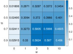
(a) Average PMI score on the
Introduction dataset.

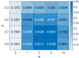
(b) Average PMI score on the
Lectures dataset.

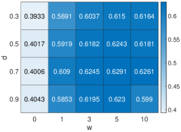
(c) Average PMI score on the
Textbook dataset.

Figure 6. Heatmaps for average PMI scores across the the documents in Introduction, Lectures and Textbook dataset with varying $w$ and $d$. We see that $w=5,d=0.7$ leads to the highest PMI scores, consistent with our choices from visually inspecting Figure 3.

We note that because BATS prevents overlapping words by design, it will achieve a similarity score of $0$ for both Jacc and Dice. For this reason, we will not use these metrics to claim that BATS has the “best” performance on the topic modeling task (the difference between “low overlap” and “no overlap” is not likely important). Instead, we include Jacc and Dice for BATS and the baselines to provide a more holistic picture of the baselines. As some baselines will have a high Jacc or Dice score as well as strong performance on other metrics, these scores highlight a potential tradeoff between low overlap and high performance on the coherence metrics. As a result, we also define composite metrics for evaluation which penalize the coherence scores on pairs of topics according to the similarity scores. Specifically, using ${\tt PMI}_{i}$ and ${\tt UMass}_{i}$ as the coherence scores for topic $i$ and ${\tt sim}_{i,j}$ as the similarity score between topics $i$ and $j$ according to Jacc or Dice, we compute:

(18) $$PMI^{sim}=\frac{\sum^{k}_{i=1}\sum^{k}_{j=1}({\tt PMI}_{i}+{\tt PMI}_{j})(1-(\operatorname{sgn}({\tt PMI}_{i}+{\tt PMI}_{j}){\tt sim}_{i,j}))/2}{k^{2}},$$

(19) $$UMass^{sim}=\frac{\sum^{k}_{i=1}\sum^{k}_{j=1}({\tt UMass}_{i}+{\tt UMass}_{j})(1+{\tt sim}_{i,j})/2}{k^{2}},$$

where $k$ refers to the total number of topics and $\operatorname{sgn}(x)$ is the sign function that evaluates to 1 if $x\geq 0$ and -1 if $x<0$. (18) uses the $\operatorname{sgn}$ function to ensure that pairs of topics with high similarity scores are penalized regardless of the sign of the sum of their PMI scores. Because the UMass scores are always negative, we can simplify this penalty to $1+{\tt sim}_{i,j}$ in (19).

4.2.3. Hyperparameter analysis

In Section 3.3.3, we determined values for $w$ and $d$ based on visually inspecting heatmaps of pairwise distances between the SVD sentence vectors. We now test these parameters against the PMI metric to validate our choices on the topic modeling task. Looking at Table 6, we can see that the best choices of $w$ and $d$ are (i) consistent with our earlier analysis (i.e., $d\approx 0.7$, $w=3$ or $5$) and (ii) reasonably consistent across datasets. This validates the idea that BATS can be fully unsupervised, where we do not have an initial training procedure for hyperparameters.

Additionally, for completeness, we study the impact of changing $\mathcal{K}$ in the PMI score across the Textbook, Lectures, and Introduction datasets for BATS. The results are shown in Table 2. We find that increasing $\mathcal{K}$ decreases the PMI score: this makes intuitive sense because as the number of words in the topics increases, less relevant words should be included, if the words within each topic are ranked effectively. In BATS, our ranking is done according to the TF-IDF scores.

4.2.4. Results and discussion

The results obtained by each algorithm on the five datasets are given in Table 3. We present the mean and standard deviations on topic diversity, topic coherence, and the four cases of joint metrics. The first two columns, Jacc and Dice, indicate the diversities of the topics (smaller being better). The following columns then give the topic coherence scores, PMI and UMass (larger being better), followed by their combinations with the similarity measures (e.g., $PMI^{Dice}$ is PMI with Dice used for ${\tt sim}_{ij}$ in (18)).

Table 3. Performance of each algorithm on the Textbook, Lectures, Introductions, Wiki, and News datasets in terms of topic coherence, similarity, and composite metrics. Our algorithm has the highest performance on most of the metrics, indicating it achieves the best balance between topic coherence and diversity.

Textbook Dataset
	Jacc	Dice	PMI	$PMI^{Jacc}$	$PMI^{Dice}$	UMass	$UMass^{Jacc}$	$UMass^{Dice}$
LDA	$\mathbf{0.00\pm 0.00}$	$\mathbf{0.00\pm 0.00}$	$-0.71\pm 0.91$	$-0.71\pm 0.91$	$-0.71\pm 0.91$	$-14.74\pm 2.78$	$-14.74\pm 2.78$	$-14.74\pm 2.78$
HDP	$0.01\pm 0.01$	$0.02\pm 0.02$	$-6.18\pm 0.86$	$-6.24\pm 1.04$	$-6.29\pm 1.05$	$-22.30\pm 0.61$	$-22.52\pm 0.68$	$-22.72\pm 0.80$
LSA	$0.28\pm 0.10$	$0.42\pm 0.13$	$\mathbf{0.65\pm 0.89}$	$0.36\pm 0.73$	$0.22\pm 0.72$	$-8.11\pm 2.21$	$-10.38\pm 2.96$	$-11.49\pm 3.30$
pLSA	$0.10\pm 0.09$	$0.14\pm 0.12$	$-3.63\pm 1.52$	$-3.97\pm 1.63$	$-4.14\pm 1.72$	$-14.65\pm 2.82$	$-16.06\pm 3.34$	$-16.78\pm 3.77$
NMF	$0.21\pm 0.10$	$0.31\pm 0.13$	$-1.69\pm 1.41$	$-1.45\pm 1.19$	$-1.32\pm 1.11$	$-13.41\pm 2.82$	$-15.94\pm 3.99$	$-17.22\pm 4.28$
SeaNMF	$0.02\pm 0.05$	$0.05\pm 0.08$	$0.26\pm 0.65$	$0.24\pm 0.64$	$0.23\pm 0.63$	$\mathbf{-6.64\pm 1.81}$	$\mathbf{-6.85\pm 2.06}$	$\mathbf{-7.01\pm 2.24}$
BATS	$\mathbf{0.00\pm 0.00}$	$\mathbf{0.00\pm 0.00}$	$0.62\pm 0.63$	$\mathbf{0.62\pm 0.63}$	$\mathbf{0.62\pm 0.63}$	$-10.28\pm 2.31$	$-10.28\pm 2.31$	$-10.28\pm 2.31$
Lectures Dataset
	Jacc	Dice	PMI	$PMI^{Jacc}$	$PMI^{Dice}$	UMass	$UMass^{Jacc}$	$UMass^{Dice}$
LDA	$\mathbf{0.00\pm 0.00}$	$\mathbf{0.00\pm 0.00}$	$-0.71\pm 0.85$	$-0.71\pm 0.85$	$-0.71\pm 0.85$	$-14.60\pm 2.52$	$-14.60\pm 2.52$	$-14.60\pm 2.52$
HDP	$0.01\pm 0.01$	$0.01\pm 0.01$	$-6.89\pm 0.69$	$-6.28\pm 0.76$	$-6.32\pm 0.77$	$-21.55\pm 0.34$	$-21.72\pm 0.37$	$-21.86\pm 0.42$
LSA	$0.27\pm 0.07$	$0.41\pm 0.09$	$\mathbf{0.59\pm 0.62}$	$0.35\pm 0.53$	$0.24\pm 0.49$	$\mathbf{-7.13\pm 1.76}$	$-8.97\pm 2.12$	$-9.92\pm 2.34$
pLSA	$0.04\pm 0.03$	$0.07\pm 0.04$	$-6.4\pm 0.77$	$-6.7\pm 0.86$	$-6.9\pm 0.94$	$-19.44\pm 0.78$	$-20.27\pm 1.04$	$-20.90\pm 1.31$
NMF	$0.26\pm 0.08$	$0.39\pm 0.10$	$0.48\pm 0.52$	$0.30\pm 0.46$	$0.21\pm 0.44$	$-9.07\pm 2.30$	$-11.39\pm 2.84$	$-12.51\pm 3.10$
SeaNMF	$0.02\pm 0.03$	$0.04\pm 0.06$	$0.26\pm 0.41$	$0.21\pm 0.40$	$0.19\pm 0.40$	$-8.36\pm 1.16$	$\mathbf{-8.49\pm 1.18}$	$\mathbf{-8.59\pm 1.20}$
BATS	$\mathbf{0.00\pm 0.00}$	$\mathbf{0.00\pm 0.00}$	$0.54\pm 0.53$	$\mathbf{0.54\pm 0.53}$	$\mathbf{0.54\pm 0.53}$	$-9.08\pm 1.82$	$-9.08\pm 1.82$	$-9.08\pm 1.82$
Introductions Dataset
	Jacc	Dice	PMI	$PMI^{Jacc}$	$PMI^{Dice}$	UMass	$UMass^{Jacc}$	$UMass^{Dice}$
LDA	$\mathbf{0.00\pm 0.00}$	$\mathbf{0.00\pm 0.00}$	$-2.09\pm 0.84$	$-2.09\pm 0.84$	$-2.09\pm 0.84$	$-15.38\pm 1.72$	$-15.38\pm 1.72$	$-15.38\pm 1.72$
HDP	$0.01\pm 0.01$	$0.01\pm 0.02$	$-7.13\pm 1.14$	$-7.17\pm 1.44$	$-7.21\pm 1.14$	$-21.78\pm 1.61$	$-21.92\pm 1.61$	$-22.04\pm 1.62$
LSA	$0.21\pm 0.09$	$0.31\pm 0.12$	$-0.64\pm 0.73$	$-0.84\pm 0.88$	$-0.93\pm 0.94$	$-8.11\pm 2.03$	$-9.88\pm 2.77$	$-10.77\pm 3.11$
pLSA	$0.04\pm 0.05$	$0.06\pm 0.07$	$-5.35\pm 1.43$	$-5.54\pm 1.46$	$-5.67\pm 1.49$	$-16.15\pm 2.29$	$16.76\pm 2.39$	$-17.16\pm 2.56$
NMF	$0.21\pm 0.08$	$0.32\pm 0.11$	$-2.16\pm 1.15$	$-2.56\pm 1.34$	$-2.76\pm 1.43$	$-14.18\pm 2.32$	$-17.05\pm 2.61$	$-18.50\pm 2.85$
SeaNMF	$0.01\pm 0.02$	$0.02\pm 0.05$	$0.38\pm 0.35$	$0.36\pm 0.36$	$0.35\pm 0.42$	$-8.18\pm 0.85$	$-8.23\pm 0.86$	$-8.27\pm 0.87$
BATS	$\mathbf{0.00\pm 0.00}$	$\mathbf{0.00\pm 0.00}$	$\mathbf{0.58\pm 0.45}$	$\mathbf{0.58\pm 0.45}$	$\mathbf{0.58\pm 0.45}$	$\mathbf{-7.69\pm 1.63}$	$\mathbf{-7.69\pm 1.63}$	$\mathbf{-7.69\pm 1.63}$
Wiki Dataset
	Jacc	Dice	PMI	$PMI^{Jacc}$	$PMI^{Dice}$	UMass	$UMass^{Jacc}$	$UMass^{Dice}$
LDA	$\mathbf{0.00\pm 0.00}$	$\mathbf{0.00\pm 0.00}$	$-3.55\pm 1.12$	$-3.55\pm 1.12$	$-3.55\pm 1.12$	$-19.14\pm 2.20$	$-19.14\pm 2.20$	$-19.14\pm 2.20$
HDP	$0.027\pm 0.02$	$0.05\pm 0.04$	$-5.98\pm 1.06$	$-6.13\pm 1.03$	$-6.25\pm 1.01$	$-22.18\pm 1.04$	$-22.77\pm 0.99$	$-23.28\pm 1.12$
LSA	$0.19\pm 0.10$	$0.29\pm 0.13$	$-0.05\pm 1.28$	$-0.30\pm 1.21$	$-0.43\pm 1.21$	$-8.11\pm 2.03$	$-9.88\pm 2.77$	$-10.77\pm 3.11$
pLSA	$0.12\pm 0.09$	$0.17\pm 0.12$	$-1.97\pm 1.63$	$-2.30\pm 1.77$	$-2.46\pm 1.87$	$-13.44\pm 3.57$	$-15.05\pm 4.29$	$-15.85\pm 4.73$
NMF	$0.14\pm 0.09$	$0.21\pm 0.14$	$-2.60\pm 1.64$	$-3.04\pm 1.08$	$-3.28\pm 1.91$	$-16.81\pm 2.85$	$-19.63\pm 3.15$	$-21.22\pm 3.49$
SeaNMF	$0.01\pm 0.03$	$0.01\pm 0.06$	$0.37\pm 0.28$	$0.36\pm 0.26$	$0.35\pm 0.22$	$-7.02\pm 0.85$	$-7.13\pm 0.92$	$-8.27\pm 0.92$
BATS	$\mathbf{0.00\pm 0.00}$	$\mathbf{0.00\pm 0.00}$	$\mathbf{0.44\pm 0.24}$	$\mathbf{0.44\pm 0.24}$	$\mathbf{0.44\pm 0.24}$	$\mathbf{-6.08\pm 0.63}$	$\mathbf{-6.08\pm 0.63}$	$\mathbf{-6.08\pm 0.63}$
News Dataset
	Jacc	Dice	PMI	$PMI^{Jacc}$	$PMI^{Dice}$	UMass	$UMass^{Jacc}$	$UMass^{Dice}$
LDA	$\mathbf{0.00\pm 0.00}$	$\mathbf{0.00\pm 0.00}$	$-2.88\pm 1.32$	$-2.88\pm 1.32$	$-2.88\pm 1.32$	$-18.77\pm 2.14$	$-18.77\pm 2.14$	$-18.77\pm 2.14$
HDP	$0.03\pm 0.03$	$0.07\pm 0.06$	$-5.25\pm 1.48$	$-5.42\pm 1.46$	$-5..56\pm 1.46$	$-21.71\pm 1.36$	$-22.52\pm 1.25$	$-23.19\pm 1.42$
LSA	$0.15\pm 0.09$	$0.24\pm 0.12$	$0.68\pm 1.46$	$0.46\pm 1.45$	$0.32\pm 1.45$	$-8.76\pm 3.77$	$-9.08\pm 3.76$	$-9.63\pm 3.75$
pLSA	$0.11\pm 0.09$	$0.16\pm 0.12$	$-1.46\pm 2.04$	$-1.78\pm 2.15$	$-1.92\pm 2.24$	$-12.37\pm 4.05$	$-13.82\pm 4.86$	$-14.54\pm 5.29$
NMF	$0.17\pm 0.08$	$0.27\pm 0.11$	$-2.03\pm 1.52$	$-2.40\pm 1.63$	$-2.60\pm 1.70$	$-17.21\pm 2.84$	$-20.14\pm 3.20$	$-21.78\pm 3.51$
SeaNMF	$0.03\pm 0.06$	$0.04\pm 0.09$	$0.69\pm 1.81$	$0.65\pm 1.80$	$0.64\pm 1.80$	$-8.92\pm 2.92$	$-9.12\pm 2.97$	$-9.20\pm 2.98$
BATS	$\mathbf{0.00\pm 0.00}$	$\mathbf{0.00\pm 0.00}$	$\mathbf{0.76\pm 1.49}$	$\mathbf{0.76\pm 1.49}$	$\mathbf{0.76\pm 1.49}$	$\mathbf{-7.56\pm 2.73}$	$\mathbf{-7.56\pm 2.73}$	$\mathbf{-7.56\pm 2.73}$

Overall, we see that compared with the baselines, our method BATS obtains competitive topic coherence scores, the lowest similarity scores, and the best composite scores in most cases. For the Introductions, Wiki, and News datasets, which are the three largest we consider, our method maintains higher performance than all baselines in all metrics. On the Textbook and Lectures datasets, BATS achieves the best performance on the PMI composite metrics and is a close second to LSA on the non-composite PMI. BATS performs second only to SeaNMF for the UMass composite metrics and comparably to the best baselines on the non-composite UMass metric. The baseline which tends to outperform our algorithm in terms of topic coherence, LSA, also performs the worst in terms of topic diversity. To interpret this diversity performance, we note that a Jacc score of $0.25$ and a Dice score of $0.4$ correspond roughly to $|T_{i}\cap T_{j}|\propto 0.4$ in (17), i.e., a 40% duplication between topics. Thus, LSA (as well as NMF) usually has up to 40% average overlap in topic words, leading to confusing topics, while our method yields no noticeable overlap. On the other hand, the baseline which matches our algorithm in topic diversity, LDA, is among the lowest performing in terms of coherence, which is also reflected in the composite metrics.

Although SeaNMF achieves both a high topic diversity score and UMass score, on the PMI metric it falls substantially short of BATS (for all datasets) and LSA (for the Textbook and Lectures datasets). This may be due to the fact that, for our purposes, the UMass score for each document is focused only on topics in that document whereas the PMI score includes information from the rest of the dataset. We can thus conclude that, among the algorithms tested, our algorithm finds the best balance between topic coherence and diversity for single document topic modeling; its consistent performance across the datasets also shows that it is robust to variations in dataset properties.

We also observe an interesting pattern in the baselines: the spectral methods – LSA and NMF – perform high in coherence but low in similarity, while the generative models – LDA and pLSA – have the opposite trends. While spectral approaches can extract topics that are interpretable when taken individually, there is high similarity between them because they are based on matrix decomposition and do not consider diversity. Generative models can extract diversified topics, but when they are operating on single documents with few word co-occurrences, the resulting topics will not be as coherent. These observations are consistent with Figure 4.

4.3. Text Segmentation

4.3.1. Baselines

We compared BATS against six baselines for the text segmentation task:

(i) TextTiling (Hearst, 1997): TextTiling divides the text into pseudosentences, assigns similarity scores at the gaps, detects peak differences in the scores, and marks the peaks as boundaries. The boundaries are normalized to the closest sentence breaks. We use the implementation from the nltk package.

(ii) C99 (Choi, 2000): C99 is another popular text segmentation algorithm that inserts boundaries based on average inter-sentence similarities. More specifically, a ranking transformation is performed, pairwise cosine distances between sentences are computed based on the ranking, and boundaries are determined based on these similarities. We implement C99 de-novo in Python.

(iii) Modified DP Algorithm with LDA (LDA_MDP) (Misra et al., 2011): LDA_MDP performs text segmentation based the LDA topic model, with the segmentation being implemented with dynamic processing (DP) techniques. The method has also been tested using an alternate topic model, multinomial mixture, but LDA has has been found to obtain better performance. We implement the LDA_MDP model de-novo in Python.

(iv) TopicTiling (Riedl and Biemann, 2012): TopicTiling is based on TextTiling, with additionally integrated topic information from the LDA topic model for text segmentation. We implement TopicTiling de-novo in Python, using a window size of 2 and 500 iterations.

(v) SupervisedSeg (Koshorek et al., 2018): SupervisedSeg formulates text segmentation as a supervised learning task, training a hierarchical bidirectional neural LSTM model on the WIKI-727K dataset. The authors transform the text into word embeddings using the GoogleNews word2vec pre-trained model, and use the word embeddings as inputs to the neural model. SupervisedSeg then predicts a cut-off probability for each sentence. We used the open source pre-trained model available from (Koshorek et al., 2018).

(vi) BERTSeg: To test the efficacy of pre-trained models, we designed BERTSeg, an algorithm that leverages the state-of-the-art Bidirectional Encoder Representations from Transformers (BERT) (Devlin et al., 2018) contextualized word embeddings for text segmentation. As the name suggests, BERT uses the Transformer deep learning architecture (Vaswani et al., 2017) to learn representations of words from unlabeled text, considering both the right context and left context in every layer (i.e., learning bidirectionally). BERTSeg is based on the open source Pytorch BERT model (Reimers and Gurevych, 2019). After using the pre-trained BERT model to generate sentence embeddings, BERTSeg employs the agglomerative segment clustering method from BATS to convert the sentence embeddings into segments.

To say consistent across the algorithms, for the topic-based text segmentation methods – LDA_MDP and TopicTiling – we train the topic model with the single document being segmented.

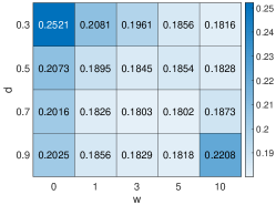
(a) Average WD score on the
Introduction dataset.

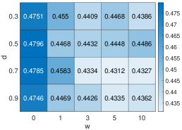
(b) Average WD score on the
Lectures dataset.

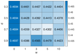
(c) Average WD score on the
Textbook dataset.

Figure 7. Heatmaps for average WD scores across the the documents in Introduction, Lectures and Textbook dataset with varying $w$ and $d$. We find that $w=5,d=0.7$ leads to the best performance, consistent with the PMI results in Figure 6.

4.3.2. Evaluation metrics

We consider two standard text segmentation metrics, $P_{k}$ (Beeferman et al., 1999) and WindowDiff (WD) (Pevzner and Hearst, 2002). Lower values indicate better performance. Each of these metrics compares the ground truth (i.e., reference) segmentation ref to the estimated (i.e., hypothesized) segmentation hyp. The $P_{k}$ metric calculates the number of disagreements in the positions of segment boundaries between hyp and ref; in doing so, it ignores the exact number of boundaries to be detected, and weights false positives more heavily (Pevzner and Hearst, 2002). WD, on the other hand, slides a fixed-sized window across the document, calculates the number of boundaries within that window, and records an error if ref and hyp disagree on the number.

Formally, let $(x_{1},x_{2},...,x_{N})$ be the sequence of $N$ words comprising a document, where each $x_{i}\in\mathcal{W}$, the set of document words. With $\delta_{z}(i,j)$ as the binary indicator of whether words $x_{i}$ and $x_{j}$ are in the same segment under segmentation $z$, and $b_{z}(i,j)$ as the number of segment boundaries between $x_{i}$ and $x_{j}$ under $z$, the metrics are calculated as

(20) $$P_{k}=\frac{1}{N-\ell}\sum_{i=1}^{N-\ell}\mathbbm{1}\{|\delta_{{\tt hyp}}(i,i+\ell)-\delta_{{\tt ref}}(i,i+\ell)|>0\},$$

(21) $$\mbox{WD}=\frac{1}{N-\ell}\sum_{i=1}^{N-\ell}\mathbbm{1}\{|b_{{\tt hyp}}(i,i+\ell)-b_{{\tt ref}}(i,i+\ell)|>0\},$$

where the window size $\ell$ is set to one less than half the average segment length, and $\mathbbm{1}$ is the indicator function which evaluates to $1$ if the argument is true and $0$ otherwise.

4.3.3. Hyperparameter analysis

We now test $w$ and $d$ against the WD metric to validate our choices on the topic modeling task. Looking at Table 7, we can see that our results are consistent with those in Section 4.2.3: the optimal values are $d\approx 0.7$, $w=3$ or $5$ for each of the datasets. Taken together, all of these results support the idea that we can use this set of parameters as default, across different datasets and evaluation metrics. This allows users to use BATS “out of the box” without fine-tuning which may be difficult due to limited data in the “new and single document” setting or computationally burdensome when data is available.

4.3.4. Results and discussion

The results obtained by each algorithm on each of the four datasets are given in Table 4. The mean and standard deviation across documents is shown in each case.

Table 4. Text segmentation evaluation metrics obtained on six datasets. Lower scores are better for both metrics. Our method outperforms the baselines in most cases (particularly for the Lectures dataset), except for BERTSeg and C99 on the Choi dataset and C99 on the Wiki dataset.

[b] Textbook Dataset Lectures Dataset Introductions Dataset Choi Dataset $P_{k}$ WD $P_{k}$ WD $P_{k}$ WD $P_{k}$ WD TextTiling $0.45\pm 0.177$ $0.47\pm 0.169$ $0.43\pm 0.099$ $0.48\pm 0.088$ $0.29\pm 0.158$ $0.33\pm 0.170$ $0.33\pm 0.076$ $0.34\pm 0.075$ C99 $0.55\pm 0.142$ $0.79\pm 0.206$ $0.51\pm 0.075$ $0.85\pm 0.164$ $0.20\pm 0.120$ $0.29\pm 0.184$ $0.14\pm 0.077$ $0.15\pm 0.081$ LDA_MDP $0.52\pm 0.161$ $0.60\pm 0.121$ $0.53\pm 0.117$ $0.63\pm 0.118$ $0.51\pm 0.142$ $0.59\pm 0.136$ $0.49\pm 0.079$ $0.50\pm 0.088$ TopicTiling $0.50\pm 0.157$ $0.56\pm 0.140$ $0.51\pm 0.110$ $0.56\pm 0.100$ $0.50\pm 0.138$ $0.57\pm 0.122$ $0.45\pm 0.079$ $0.47\pm 0.082$ SupervisedSeg $0.45\pm 0.157$ $0.58\pm 0.180$ $0.42\pm 0.096$ $\mathbf{0.43\pm 0.083}$ $0.45\pm 0.127$ $0.57\pm 0.133$ $0.23\pm 0.064$ $0.24\pm 0.065$ BERTSeg $0.41\pm 0.193$ $0.44\pm 0.181$ $0.43\pm 0.148$ $0.47\pm 0.158$ $0.17\pm 0.149$ $0.19\pm 0.163$ $\mathbf{0.10\pm 0.074}$ $\mathbf{0.11\pm 0.076}$ BATS $\mathbf{0.41\pm 0.162}$ $0.43\pm 0.164$ $0.38\pm 0.112$ $0.43\pm 0.112$ $0.16\pm 0.136$ $0.18\pm 0.143$ $0.22\pm 0.103$ $0.23\pm 0.109$ Wiki Dataset News Dataset $P_{k}$ WD $P_{k}$ WD TextTiling $0.39\pm 0.123$ $0.41\pm 0.122$ $0.42\pm 0.154$ $0.44\pm 0.153$ C99 $\mathbf{0.37\pm 0.126}$ $\mathbf{0.38\pm 0.124}$ $0.39\pm 0.157$ $0.40\pm 0.158$ LDA_MDP $0.62\pm 0.124$ $0.68\pm 0.136$ $0.64\pm 0.142$ $0.69\pm 0.130$ TopicTiling $0.46\pm 0.141$ $0.48\pm 0.146$ $0.43\pm 0.154$ $0.45\pm 0.153$ SupervisedSeg $0.42\pm 0.145$ $0.44\pm 0.147$ $0.41\pm 0.151$ $0.43\pm 0.154$ BERTSeg $0.40\pm 0.149$ $0.41\pm 0.152$ $0.36\pm 0.113$ $0.38\pm 0.114$ BATS $0.39\pm 0.148$ $0.41\pm 0.145$ $\mathbf{0.34\pm 0.155}$ $\mathbf{0.36\pm 0.157}$

Overall, we see that our method BATS consistently outperforms all of the baselines in terms of text segmentation on four of out of six datasets. BERTSeg is the most competitive on the baseline on all of the datasets except for Lectures, where SupervisedSeg does slightly better, and Wiki where C99 performs better. The three topic-based text segmentation methods (LDA_MDP, and TopicTiling) actually perform considerably worse than these other baselines, possibly due to single documents containing insufficient data for training their topic models (recall in particular that LDA had poor topic diversity performance in Table 4). Although for the Textbook and Introductions datasets BATS achieves only modest gains over BERTSeg, this achievement is noteworthy as BERT is very large (around 335 million parameters) and, even pre-trained, has a runtime two orders of magnitude worse than BATS (see Section 4.4). The performance gains are more pronounced in the Lectures and News datasets where BATS improves more substantially on BERTSeg.

The pre-trained models outperforming the simpler baselines is perhaps not surprising. However, the fact that they achieve comparable but slightly worse results than BATS across three natural datasets suggests that (i) given their computational complexity, pre-trained embedding models are not as well suited for the “new and single document” setting as BATS, and (ii) the relatively simple and efficient pre-processing and biclustering techniques of BATS in combination are effective. Considering these results along with those in in Sec. 4.2, we conclude that our method is capable of identifying accurate segment boundaries and topic words for a single document simultaneously.

The C99 baseline performs remarkably well on the Choi and Wiki datasets. C99 is designed specifically with datasets such as Choi in mind, where documents are artificially built with identical numbers of short segments and sparse content in each segment (Choi, 2000). Specifically, as shown in Table 1, the average sentences per document in Choi are significantly smaller than the other datasets. This is due to the way it is constructed – with each document as combinations of first $\ell$ sentences from documents in another corpus – making it less realistic than the other datasets. Similarly, because BERTSeg uses agglomerative clustering on pre-trained embeddings directly (instead of using embeddings as input to another supervised model), it may be particularly apt for identifying breaks among unrelated topics (i.e., topics from different articles) as opposed to the harder task of segmenting natural text with related topics. Put simply, using the embeddings directly makes a “coarse” separation between unrelated topics easier as word embeddings are designed to capture these semantic differences. By contrast, BATS is designed to segment natural text with a “finer” separation between topics that are related but distinct in the “single and new document” setting. In this setting, even contextualized embeddings are not as effective as the semantic differences between topics is likely to be relatively small and so BATS outperforms embeddings-based models, as evidenced by results on the other datasets. Similar results have been observed in, e.g., (Koshorek et al., 2018).

4.4. Scalability Analysis

Next, we evaluate the effect of the number of sentences and segments on the runtime of our method compared with the baselines. Table 5 shows the increase in runtime from varying the number of sentences in each segment for the Choi dataset, relative to the case of 50 sentences (we choose this dataset because all documents are constructed with a constant number of segments). We can see that the growth in runtime of our methodology BATS is comparable to the most scalable baselines, with the rate of increase in runtime less than the corresponding increase in sentences. Additionally, BATS is the only methodology performing both topic modeling and text segmentation. Out of the baselines in Table 5, TextTiling, C99, and pLSA have considerably higher increases in runtime, with pLSA performing the worst. The substantial difference between LSA, the most scalable, and pLSA is consistent with spectral approaches being known to scale better than generative algorithms that require multiple iterations (Zhong and Ghosh, 2005). Although BERTSeg and SupervisedSeg scale relatively well, they have absolute runtimes second and third to pLSA for all sentence lengths. This indicates that there is a high fixed overhead associated with loading the large pre-trained models for segmentation.

Table 5. Absolute running time and increasing rate when varying the number of sentences in the Choi dataset. The time increase is relative to the case of 50 sentences. Our method scales well compared with the baselines.

Sentences 50 (baseline) 60 80 100 120 140 Runtime Abs. Abs. Rate Abs. Rate Abs. Rate Abs. Rate Abs. Rate LSA 5.21 6.15 1.18 7.24 1.39 8.53 1.64 9.54 1.83 10.62 2.04 NMF 35.63 43.72 1.23 56.81 1.59 64.65 1.81 86.71 2.43 92.79 2.60 HDP 89.6 109.12 1.22 137.78 1.54 179.55 2.00 202.35 2.26 238.98 2.67 TopicTiling 55.02 67.63 1.23 87.69 1.59 109.95 2.00 125.56 2.28 148.61 2.70 LDA_MDP 931.26 1130.78 1.21 1446.27 1.55 1843.17 1.98 2022.65 2.17 2598.78 2.79 LDA 837.8 1078.98 1.29 1342.06 1.60 1710.25 2.04 2085.36 2.49 2395.94 2.86 TextTiling 90.12 140.18 1.56 227.75 2.53 349.76 3.88 447.13 4.96 639.63 7.10 C99 28.42 44.32 1.56 74.21 2.61 119.24 4.20 172.44 6.07 227.15 7.99 pLSA 14742.62 23388.19 1.59 39804.17 2.70 64856.58 4.40 90536.42 6.14 125231.36 8.49 SupervisedSeg 2103.45 2615.49 1.24 2676.45 1.27 3419.84 1.63 4350.65 2.07 4727.54 2.25 BERTSeg 5361.82 7616.14 1.42 8522.98 1.59 9663.25 1.80 12324.16 2.30 13193.24 2.46 SeaNMF 79.46 85.67 1.08 114.27 1.44 140.79 1.77 152.14 1.91 206.71 2.60 BATS 52.49 60.29 1.15 69.71 1.33 89.84 1.71 95.75 1.82 109.62 2.09

Table 6. The absolute running time and increasing rate for text segments in the Lectures dataset with the varying number of segments. The baseline is 10 segments, and each bar is over 10 runs.

Segments 10 (baseline) 20 30 40 50 Runtime Abs. Rate Abs. Rate Abs. Rate Abs. Rate Abs. Rate HDP 1105.63 1 1104.4 1 1104.12 1 1104.41 1 1105.45 1 LDA 4272.27 1 4272.86 1 4319.22 1.01 4381.64 1.03 4453.33 1.04 LSA 225.94 1 266.43 1.18 289.98 1.28 303.22 1.34 312.37 1.38 NMF 491.57 1 570 1.16 647.43 1.32 739.32 1.5 840.84 1.71 SeaNMF 526.38 1 950.87 1.81 1211.23 2.3 1370.74 2.6 2299.02 4.37 BATS 2434.27 1 2448.87 1.01 2469.49 1.01 2493.14 1.02 2517.15 1.03 Segments 60 70 80 90 100 Runtime Abs. Rate Abs. Rate Abs. Rate Abs. Rate Abs. Rate HDP 1108.22 1 1111.68 1.01 1115.45 1.01 1119.19 1.01 1122.55 1.02 LDA 4518.03 1.06 4576.03 1.07 4629.34 1.08 4678.3 1.1 4722.8 1.11 LSA 316.39 1.4 320.22 1.42 323.86 1.43 327.44 1.45 330.99 1.46 NMF 888.14 1.81 934.04 1.9 982.02 2 1033.77 2.1 1090.05 2.22 SeaNMF 3167.22 6.02 4235.9 8.05 6324.47 12.02 7827.73 14.87 8692.67 16.51 BATS 2540.81 1.04 2564.17 1.05 2587.01 1.06 2609.59 1.07 2632.07 1.08

Table 6 shows the impact on runtime from varying the number of segments per document for the Lectures dataset (recall from Table 1 this dataset has the longest documents available). Here we have excluded pLSA, as its runtime is significantly longer, and also the text segmentation baselines, as their runtimes are not dependent on the number of segments. SeaNMF is by far impacted the most, followed by NMF and LSA, while HDP and LDA exhibit the best scalability. Our method remains impacted under 10% for a $5$-fold increase in segments, again implying that our method supports changes in the size of input efficiently. We note that while for a small number of topics BATS has a longer absolute runtime than SeaNMF, this disadvantage disappears when the number of segments exceeds 50. Taken together, Tables 5 and 6 validate our theoretical analysis in Section 3.6 which concluded that BATS has low computational complexity.

When we consider these runtime results in the context of the evaluation metrics, we find that BATS provides the best balance of computational efficiency and performance across evaluation metrics for both the text segmentation and the topic modeling tasks. When compared with the most competitive topic modeling baselines (LSA and SeaNMF), BATS is not as efficient as LSA but scores much better on topic similarity measures. BATS scales better than SeaNMF and has a significantly lower runtime on longer documents with many segments, as evidenced by its performance on the Lectures dataset (Table 6). On the text segmentation task, BATS both scales better and has a much lower absolute running time than the two best baselines (BERTSeg and SupervisedSeg) in addition to outperforming both of them on three real-world datasets. These results show that BATS is a practical algorithm with substantial advantages over existing baselines for the “single and new document” setting that we are focused on in this paper.

4.5. Ablation Study

To test the effectiveness of different parts of the BATS methodology, we conduct an ablation study that excludes components and measures the resulting performance effect. The results for both the topic coherence and text segmentation metrics are given in Table 7. Referring to Figure 1, we focus on the following parts of BATS: (i) parts of speech (POS) awarding (i.e., setting $\lambda=0$ in (1)), (ii) low frequency processing (i.e., not excluding degree one words), (iii) regularization of the graph Laplacian (i.e., setting the $\tau$ terms to $0$ in (3)), (iv) sentence bonding (i.e., setting $d=0$ in (2)), and (v) the Laplacian. For (v), we remove the Laplacian entirely, and instead perform SVD directly on the sentence-word matrix after POS awarding and sentence bonding.

We draw three main conclusions from these results. First, each component of BATS has a substantial impact on one or more of the metrics, which validates its inclusion in the methodology. Second, the topic coherence metrics are impacted by each component more significantly than the text segmentation metrics, which implies that results at the sentence level are not impacted as significantly by preprocessing than those at the topic level. Third, out of all the components, the Laplacian has the greatest impact, followed by sentence bonding. This validates our graph Laplacian representation as input to the spectral clustering algorithm and suggests that our connection to denoising under the stochastic block model is appropriate. The impact of removing sentence bonding reflects the importance of incorporating word order information in the presence of sparsity.

Table 7. Ablation studies on the Textbook, Lectures, and Introduction datasets. Each row gives the performance on metrics obtained when excluding a component of the methodology. Overall, we see that each component is important to BATS, as excluding any of them results in lower performance on one or more metrics.

Textbook Dataset Lectures Dataset PMI UMass $P_{k}$ WD PMI UMass $P_{k}$ WD BATS - SPEECH $0.42\pm 0.74$ $-11.21\pm 2.44$ $0.42\pm 0.18$ $0.44\pm 0.17$ $0.29\pm 0.55$ $-9.88\pm 2.05$ $0.42\pm 0.16$ $0.44\pm 0.16$ BATS - FREQUENCY $0.41\pm 0.75$ $-11.18\pm 2.88$ $0.42\pm 0.17$ $0.44\pm 0.16$ $0.21\pm 0.58$ $-10.79\pm 2.11$ $0.41\pm 0.11$ $0.45\pm 0.11$ BATS - REGULARIZATION $-2.25\pm 0.77$ $-14.81\pm 1.83$ $0.44\pm 0.18$ $0.45\pm 0.17$ $-2.27\pm 0.97$ $-14.99\pm 1.28$ $0.40\pm 0.12$ $0.44\pm 0.12$ BATS - BONDING $-2.38\pm 0.76$ $-14.69\pm 1.79$ $0.44\pm 0.19$ $0.47\pm 0.17$ $-2.39\pm 0.99$ $-14.80\pm 1.16$ $0.42\pm 0.13$ $0.47\pm 0.12$ BATS - LAPLACIAN $-3.46\pm 0.82$ $-16.48\pm 2.89$ $0.48\pm 0.18$ $0.51\pm 0.18$ $-3.79\pm 0.54$ $-16.11\pm 1.82$ $0.51\pm 0.14$ $0.54\pm 0.15$ BATS $\mathbf{0.62\pm 0.63}$ $\mathbf{-10.28\pm 2.31}$ $\mathbf{0.41\pm 0.16}$ $\mathbf{0.43\pm 0.16}$ $\mathbf{0.54\pm 0.53}$ $\mathbf{-9.08\pm 1.82}$ $\mathbf{0.38\pm 0.11}$ $\mathbf{0.43\pm 0.11}$ Introductions Dataset PMI UMass $P_{k}$ WD BATS - SPEECH $0.17\pm 0.45$ $-8.18\pm 1.62$ $0.163\pm 0.14$ $0.185\pm 0.15$ BATS - FREQUENCY $0.16\pm 0.47$ $-8.40\pm 1.71$ $0.164\pm 0.15$ $0.186\pm 0.16$ BATS - REGULARIZATION $0.15\pm 0.49$ $-12.09\pm 2.21$ $0.164\pm 0.14$ $0.189\pm 0.15$ BATS - BONDING $-2.25\pm 0.77$ $-14.81\pm 1.83$ $0.166\pm 0.15$ $0.188\pm 0.17$ BATS - LAPLACIAN $-2.67\pm 0.73$ $-15.21\pm 2.12$ $0.376\pm 0.10$ $0.382\pm 0.11$ BATS $\mathbf{0.58\pm 0.45}$ $\mathbf{-7.69\pm 1.63}$ $\mathbf{0.160\pm 0.14}$ $\mathbf{0.180\pm 0.14}$

5. Conclusion and Future Work

The “single and new document” setting arises when it is desirable to perform modeling tasks on a single document, due to the potential novelty of words in the document and/or computational limitations. In this work, we developed an unsupervised, computationally efficient, statistically sound methodology called BATS that simultaneously extracts the topics and segments the text from one single document. BATS first leverages word-order information together with optimization tricks such as parts-of-speech (POS) tagging to refine a document’s sentence-word matrix. It then obtains a singular value decomposition from a regularized form of the graph Laplacian, with the singular vectors yielding low dimensional embeddings of words and sentences. Finally, BATS employs clustering algorithms to extract topics and text segments from the left and right singular vectors. Through evaluations against 12 baselines on six datasets, we confirmed that our algorithm achieves the best overall results considering runtime, scalability, and standard metrics in both topic modeling and text segmentation tasks for the “single and new document” setting. For topic modeling, this was especially true when considering the dual objectives of coherence maximization and similarity minimization across topics. Our experimental results also showed that BATS scales well with the size of the input data, and that it is robust to changes in dataset characteristics.

We identify several potential avenues of future work. First, BATS could potentially be tuned to improve performance on the topic modeling or text segmentation task at the cost of increased computation. Specifically, although we found that BATS outperformed baselines based on word embedding techniques, further experimentation may leverage embeddings to enhance BATS. As this would likely come at substantial computational cost (see Tables 5 and 6), we leave this as an avenue for future work beyond the “single and new document” setting. Second, a more elaborate POS awarding scheme in the sentence-word matrix construction phase of BATS may improve topic coherence further. Third, since BATS provides both topic and text segment information, the application of our methodology to text summarization can also be considered, e.g., in identifying the most important segments according to the number of corresponding topic words.

6. Acknowledgement

We thank anonymous reviewers for helpful comments and suggestions. Christopher G. Brinton was supported in part by the Charles Koch Foundation. Qiong Wu and Zhenming Liu are supported by NSF grants NSF-2008557, NSF-1835821, and NSF-1755769. Yanhua Li was supported in part by NSF grants IIS-1942680 (CAREER), CNS-1952085, CMMI1831140, and DGE-2021871. The authors acknowledge William $\&$ Mary Research Computing for providing computational resources and technical support that have contributed to the results reported within this paper.

References

- (1)
- Amini et al. (2013) Arash A Amini, Aiyou Chen, Peter J Bickel, Elizaveta Levina, et al. 2013. Pseudo-likelihood methods for community detection in large sparse networks. The Annals of Statistics 41, 4 (2013), 2097–2122.
- Angelov (2020) Dimo Angelov. 2020. Top2Vec: Distributed Representations of Topics. arXiv preprint arXiv:2008.09470 (2020).
- Beeferman et al. (1999) Doug Beeferman, Adam Berger, and John Lafferty. 1999. Statistical models for text segmentation. Machine learning 34, 1-3 (1999), 177–210.
- Bird et al. (2009) Steven Bird, Ewan Klein, and Edward Loper. 2009. Natural language processing with Python: analyzing text with the natural language toolkit. ” O’Reilly Media, Inc.”.
- Blei et al. (2003) David M Blei, Andrew Y Ng, and Michael I Jordan. 2003. Latent dirichlet allocation. Journal of machine Learning research 3, Jan (2003), 993–1022.
- Brants et al. (2002) Thorsten Brants, Francine Chen, and Ioannis Tsochantaridis. 2002. Topic-based document segmentation with probabilistic latent semantic analysis. In Proceedings of the eleventh international conference on Information and knowledge management. ACM, 211–218.
- Brinton et al. (2018) Christopher G Brinton, Swapna Buccapatnam, Liang Zheng, Da Cao, Andrew S Lan, Felix MF Wong, Sangtae Ha, Mung Chiang, and H Vincent Poor. 2018. On the efficiency of online social learning networks. IEEE/ACM Transactions on Networking 26, 5 (2018), 2076–2089.
- Chambers. (2013) A. Chambers. 2013. Statistical models for text classification: Applications and analysis. In ProQuest Dissertations and Theses.
- Chang et al. (2009) Jonathan Chang, Sean Gerrish, Chong Wang, Jordan L Boyd-Graber, and David M Blei. 2009. Reading tea leaves: How humans interpret topic models. In Advances in neural information processing systems. 288–296.
- Chaudhuri et al. (2012) Kamalika Chaudhuri, Fan Chung, and Alexander Tsiatas. 2012. Spectral clustering of graphs with general degrees in the extended planted partition model. In Conference on Learning Theory. 35–1.
- Chiang and Zhang (2016) Mung Chiang and Tao Zhang. 2016. Fog and IoT: An overview of research opportunities. IEEE Internet of Things Journal 3, 6 (2016), 854–864.
- Choi (2000) Freddy YY Choi. 2000. Advances in domain independent linear text segmentation. arXiv preprint cs/0003083 (2000).
- Cui et al. (2019) Wanqiu Cui, Junping Du, Dawei Wang, Xunpu Yuan, Feifei Kou, Liyan Zhou, and Nan Zhou. 2019. Short Text Analysis Based on Dual Semantic Extension and Deep Hashing in Microblog. ACM Transactions on Intelligent Systems and Technology (TIST) 10, 4 (2019), 1–24.
- Daud et al. (2010) Ali Daud, Juanzi Li, Lizhu Zhou, and Faqir Muhammad. 2010. Knowledge discovery through directed probabilistic topic models: a survey. Frontiers of computer science in China 4, 2 (2010), 280–301.
- Davidson and Ravi (2005) Ian Davidson and SS Ravi. 2005. Agglomerative hierarchical clustering with constraints: Theoretical and empirical results. In European Conference on Principles of Data Mining and Knowledge Discovery. Springer, 59–70.
- Deerwester et al. (1990) Scott Deerwester, Susan T Dumais, George W Furnas, Thomas K Landauer, and Richard Harshman. 1990. Indexing by latent semantic analysis. Journal of the American society for information science 41, 6 (1990), 391–407.
- Devlin et al. (2018) Jacob Devlin, Ming-Wei Chang, Kenton Lee, and Kristina Toutanova. 2018. Bert: Pre-training of deep bidirectional transformers for language understanding. arXiv preprint arXiv:1810.04805 (2018).
- Dhillon (2001) Inderjit S Dhillon. 2001. Co-clustering documents and words using bipartite spectral graph partitioning. In ACM SIGKDD. ACM, 269–274.
- Dhillon et al. (2003) Inderjit S Dhillon, Subramanyam Mallela, and Dharmendra S Modha. 2003. Information-theoretic co-clustering. In ACM SIGKDD. ACM, 89–98.
- Eikmeier and Gleich (2017) Nicole Eikmeier and David F Gleich. 2017. Revisiting power-law distributions in spectra of real world networks. In Proceedings of the 23rd ACM SIGKDD International Conference on Knowledge Discovery and Data Mining. 817–826.
- Eisenstein and Barzilay (2008) Jacob Eisenstein and Regina Barzilay. 2008. Bayesian unsupervised topic segmentation. In Proceedings of the 2008 Conference on Empirical Methods in Natural Language Processing. 334–343.
- Elman (1990) Jeffrey L Elman. 1990. Finding structure in time. Cognitive science 14, 2 (1990), 179–211.
- Fano (1961) Robert M Fano. 1961. Transmission of information: A statistical theory of communications. American Journal of Physics 29, 11 (1961), 793–794.
- Francis and Kucera (1979) W. N. Francis and H. Kucera. 1979. Brown Corpus Manual. Technical Report. Department of Linguistics, Brown University, Providence, Rhode Island, US. http://icame.uib.no/brown/bcm.html
- Gao et al. (2017) Yang Gao, Yuefeng Li, Raymond YK Lau, Yue Xu, and Md Abul Bashar. 2017. Finding semantically valid and relevant topics by association-based topic selection model. ACM Transactions on Intelligent Systems and Technology (TIST) 9, 1 (2017), 1–22.
- Goldberg and Nivre (2012) Yoav Goldberg and Joakim Nivre. 2012. A dynamic oracle for arc-eager dependency parsing. COLING (2012), 959–976.
- Gomaa and Fahmy (2013) Wael H Gomaa and Aly A Fahmy. 2013. A survey of text similarity approaches. International Journal of Computer Applications 68, 13 (2013), 13–18.
- Hajjem and Latiri (2017) Malek Hajjem and Chiraz Latiri. 2017. Combining IR and LDA topic modeling for filtering microblogs. Procedia Computer Science 112 (2017), 761–770.
- Hearst (1997) Marti A Hearst. 1997. TextTiling: Segmenting text into multi-paragraph subtopic passages. Computational linguistics 23, 1 (1997), 33–64.
- Hofmann (2017) Thomas Hofmann. 2017. Probabilistic latent semantic indexing. In ACM SIGIR, Vol. 51. ACM, 211–218.
- Hong and Davison (2010) Liangjie Hong and Brian D Davison. 2010. Empirical study of topic modeling in twitter. In Proceedings of the first workshop on social media analytics. 80–88.
- Jarvis and Patrick (1973) Raymond Austin Jarvis and Edward A Patrick. 1973. Clustering using a similarity measure based on shared near neighbors. IEEE Transactions on computers 100, 11 (1973), 1025–1034.
- Karrer and Newman (2011) Brian Karrer and Mark EJ Newman. 2011. Stochastic blockmodels and community structure in networks. Physical review E 83, 1 (2011), 016107.
- Kluger et al. (2003) Yuval Kluger, Ronen Basri, Joseph T Chang, and Mark Gerstein. 2003. Spectral biclustering of microarray data: coclustering genes and conditions. Genome research 13, 4 (2003), 703–716.
- Koshorek et al. (2018) Omri Koshorek, Adir Cohen, Noam Mor, Michael Rotman, and Jonathan Berant. 2018. Text segmentation as a supervised learning task. arXiv preprint arXiv:1803.09337 (2018).
- Levy and Goldberg (2014) Omer Levy and Yoav Goldberg. 2014. Neural word embedding as implicit matrix factorization. Advances in neural information processing systems 27 (2014), 2177–2185.
- Li et al. (2017) Cheng Li, Felix Wong, Zhenming Liu, and Varun Kanade. 2017. From which world is your graph? arXiv preprint arXiv:1711.00982 (2017).
- Li et al. (2019) Dingcheng Li, Siamak Zamani, Jingyuan Zhang, and Ping Li. 2019. Integration of Knowledge Graph Embedding Into Topic Modeling with Hierarchical Dirichlet Process. In Proceedings of the 2019 Conference of the North American Chapter of the Association for Computational Linguistics: Human Language Technologies, Volume 1 (Long and Short Papers). 940–950.
- Li et al. (2018) Jing Li, Aixin Sun, and Shafiq R Joty. 2018. SegBot: A Generic Neural Text Segmentation Model with Pointer Network.. In IJCAI. 4166–4172.
- Lloyd (1982) Stuart Lloyd. 1982. Least squares quantization in PCM. IEEE transactions on information theory 28, 2 (1982), 129–137.
- Manabu and Takeo (1994) Okumura Manabu and Honda Takeo. 1994. Word sense disambiguation and text segmentation based on lexical cohesion. In The 15th conference on Computational linguistics-Volume 2. Association for Computational Linguistics, 755–761.
- Manning et al. (2008) Christopher D Manning, Prabhakar Raghavan, and Hinrich Schütze. 2008. Introduction to information retrieval. Cambridge university press.
- McCann et al. (2017) Bryan McCann, James Bradbury, Caiming Xiong, and Richard Socher. 2017. Learned in translation: Contextualized word vectors. In Advances in Neural Information Processing Systems. 6294–6305.
- Mikolov et al. (2013a) Tomas Mikolov, Kai Chen, Greg Corrado, and Jeffrey Dean. 2013a. Efficient estimation of word representations in vector space. arXiv preprint arXiv:1301.3781 (2013).
- Mikolov et al. (2013b) Tomas Mikolov, Ilya Sutskever, Kai Chen, Greg S Corrado, and Jeff Dean. 2013b. Distributed representations of words and phrases and their compositionality. In NeurIPS. 3111–3119.
- Mimno et al. (2011) David Mimno, Hanna M Wallach, Edmund Talley, Miriam Leenders, and Andrew McCallum. 2011. Optimizing semantic coherence in topic models. In Conference on Empirical Methods in Natural Language Processing. Association for Computational Linguistics, 262–272.
- Misra et al. (2011) Hemant Misra, François Yvon, Olivier Cappé, and Joemon Jose. 2011. Text segmentation: A topic modeling perspective. Information Processing & Management 47, 4 (2011), 528–544.
- Nguyen et al. (2015) Dat Quoc Nguyen, Richard Billingsley, Lan Du, and Mark Johnson. 2015. Improving topic models with latent feature word representations. Transactions of the Association for Computational Linguistics 3 (2015), 299–313.
- Nikolenko (2016) Sergey I Nikolenko. 2016. Topic quality metrics based on distributed word representations. In Proceedings of the 39th International ACM SIGIR conference on Research and Development in Information Retrieval. 1029–1032.
- Niwattanakul et al. (2013) Suphakit Niwattanakul, Jatsada Singthongchai, Ekkachai Naenudorn, and Supachanun Wanapu. 2013. Using of Jaccard coefficient for keywords similarity. In Proceedings of the international multiconference of engineers and computer scientists, Vol. 1. 380–384.
- Pauca et al. (2004) V Paul Pauca, Farial Shahnaz, Michael W Berry, and Robert J Plemmons. 2004. Text mining using non-negative matrix factorizations. In SIAM International Conference on Data Mining. SIAM, 452–456.
- Pennington et al. (2014) Jeffrey Pennington, Richard Socher, and Christopher Manning. 2014. Glove: Global vectors for word representation. In Proceedings of the 2014 conference on empirical methods in natural language processing (EMNLP). 1532–1543.
- Peters et al. (2017) Matthew E Peters, Waleed Ammar, Chandra Bhagavatula, and Russell Power. 2017. Semi-supervised sequence tagging with bidirectional language models. arXiv preprint arXiv:1705.00108 (2017).
- Pevzner and Hearst (2002) Lev Pevzner and Marti A Hearst. 2002. A critique and improvement of an evaluation metric for text segmentation. Computational Linguistics 28, 1 (2002), 19–36.
- Qiang et al. (2017) Jipeng Qiang, Ping Chen, Tong Wang, and Xindong Wu. 2017. Topic modeling over short texts by incorporating word embeddings. In Pacific-Asia Conference on Knowledge Discovery and Data Mining. Springer, 363–374.
- Qin and Rohe (2013) Tai Qin and Karl Rohe. 2013. Regularized spectral clustering under the degree-corrected stochastic blockmodel. In Advances in Neural Information Processing Systems. 3120–3128.
- Quan et al. (2015) Xiaojun Quan, Chunyu Kit, Yong Ge, and Sinno Jialin Pan. 2015. Short and sparse text topic modeling via self-aggregation. In Twenty-fourth international joint conference on artificial intelligence.
- Rajaraman and Ullman (2011) Anand Rajaraman and Jeffrey David Ullman. 2011. Mining of Massive Datasets: Data Mining (Ch01). Min. Massive Datasets 18 (2011), 114–142.
- Reimers and Gurevych (2019) Nils Reimers and Iryna Gurevych. 2019. Sentence-bert: Sentence embeddings using siamese bert-networks. arXiv preprint arXiv:1908.10084 (2019).
- Resnik (1993) Philip Stuart Resnik. 1993. Selection and information: a class-based approach to lexical relationships. IRCS Technical Reports Series (1993), 200.
- Riedl and Biemann (2012) Martin Riedl and Chris Biemann. 2012. TopicTiling: a text segmentation algorithm based on LDA. In ACL Student Research Workshop. Association for Computational Linguistics, 37–42.
- Röder et al. (2015) Michael Röder, Andreas Both, and Alexander Hinneburg. 2015. Exploring the space of topic coherence measures. In ACM international conference on Web search and data mining. ACM, 399–408.
- Rohe et al. (2012) Karl Rohe, Tai Qin, and Bin Yu. 2012. Co-clustering for directed graphs: the Stochastic co-Blockmodel and spectral algorithm Di-Sim. arXiv:1204.2296 (2012).
- Sarne et al. (2019) David Sarne, Jonathan Schler, Alon Singer, Ayelet Sela, and Ittai Bar Siman Tov. 2019. Unsupervised topic extraction from privacy policies. In Companion Proceedings of The 2019 World Wide Web Conference. 563–568.
- Schneider and Vlachos (2018) Johannes Schneider and Michail Vlachos. 2018. Topic modeling based on keywords and context. In Proceedings of the 2018 SIAM International Conference on Data Mining. SIAM, 369–377.
- Shi et al. (2018) Tian Shi, Kyeongpil Kang, Jaegul Choo, and Chandan K Reddy. 2018. Short-text topic modeling via non-negative matrix factorization enriched with local word-context correlations. In Proceedings of the 2018 World Wide Web Conference. 1105–1114.
- Shi et al. (2016) Weisong Shi, Jie Cao, Quan Zhang, Youhuizi Li, and Lanyu Xu. 2016. Edge computing: Vision and challenges. IEEE internet of things journal 3, 5 (2016), 637–646.
- Stathopoulos and McCombs (2010) Andreas Stathopoulos and James R McCombs. 2010. PRIMME: preconditioned iterative multimethod eigensolver—methods and software description. ACM Transactions on Mathematical Software (TOMS) 37, 2 (2010), 1–30.
- Teh et al. (2005) Yee W Teh, Michael I Jordan, Matthew J Beal, and David M Blei. 2005. Sharing clusters among related groups: Hierarchical Dirichlet processes. In Advances in neural information processing systems. 1385–1392.
- Tran et al. (2017) Tuyen X Tran, Abolfazl Hajisami, Parul Pandey, and Dario Pompili. 2017. Collaborative mobile edge computing in 5G networks: New paradigms, scenarios, and challenges. IEEE Communications Magazine 55, 4 (2017), 54–61.
- Tu et al. (2020) Yuwei Tu, Yichen Ruan, Su Wang, Satyavrat Wagle, Christopher G Brinton, and Carlee Joe-Wang. 2020. Network-Aware Optimization of Distributed Learning for Fog Computing. arXiv preprint arXiv:2004.08488 (2020).
- Vaswani et al. (2017) Ashish Vaswani, Noam Shazeer, Niki Parmar, Jakob Uszkoreit, Llion Jones, Aidan N Gomez, Łukasz Kaiser, and Illia Polosukhin. 2017. Attention is all you need. In Advances in neural information processing systems. 5998–6008.
- Von Luxburg (2007) Ulrike Von Luxburg. 2007. A tutorial on spectral clustering. Statistics and computing 17, 4 (2007), 395–416.
- Walker et al. (1990) Henry Kenneth Walker, Wilbur Dallas Hall, and John Willis Hurst. 1990. The Oral Cavity and Associated Structures–Clinical Methods: The History, Physical, and Laboratory Examinations. Butterworths.
- Wu et al. (2019) Qiong Wu, Felix Ming Fai Wong, Zhenming Liu, Yanhua Li, and Varun Kanade. 2019. Adaptive Reduced Rank Regression. arXiv preprint arXiv:1905.11566 (2019).
- Yan et al. (2013) Xiaohui Yan, Jiafeng Guo, Yanyan Lan, and Xueqi Cheng. 2013. A biterm topic model for short texts. In International conference on World Wide Web. ACM, 1445–1456.
- Yao et al. (2009) Limin Yao, David Mimno, and Andrew McCallum. 2009. Efficient methods for topic model inference on streaming document collections. In Proceedings of the 15th ACM SIGKDD international conference on Knowledge discovery and data mining. 937–946.
- Yao et al. (2017) Liang Yao, Yin Zhang, Baogang Wei, Zhe Jin, Rui Zhang, Yangyang Zhang, and Qinfei Chen. 2017. Incorporating knowledge graph embeddings into topic modeling. In Thirty-first AAAI conference on artificial intelligence.
- Yao et al. (2018) Zijun Yao, Yifan Sun, Weicong Ding, Nikhil Rao, and Hui Xiong. 2018. Dynamic word embeddings for evolving semantic discovery. In Proceedings of the eleventh acm international conference on web search and data mining. 673–681.
- Yin and Wang (2014) Jianhua Yin and Jianyong Wang. 2014. A dirichlet multinomial mixture model-based approach for short text clustering. In ACM SIGKDD. ACM, 233–242.
- Zhao et al. (2017) He Zhao, Lan Du, Wray Buntine, and Gang Liu. 2017. MetaLDA: a topic model that efficiently incorporates meta information. In 2017 IEEE International Conference on Data Mining (ICDM). IEEE, 635–644.
- Zhao et al. (2019) Jieyu Zhao, Tianlu Wang, Mark Yatskar, Ryan Cotterell, Vicente Ordonez, and Kai-Wei Chang. 2019. Gender bias in contextualized word embeddings. arXiv preprint arXiv:1904.03310 (2019).
- Zhao et al. (2011) Wayne Xin Zhao, Jing Jiang, Jianshu Weng, Jing He, Ee-Peng Lim, Hongfei Yan, and Xiaoming Li. 2011. Comparing twitter and traditional media using topic models. In European conference on information retrieval. Springer, 338–349.
- Zhong and Ghosh (2005) Shi Zhong and Joydeep Ghosh. 2005. Generative model-based document clustering: a comparative study. Knowledge and Information Systems 8, 3 (2005), 374–384.
- Zipf (1949) George Kingsley Zipf. 1949. Human behavior and the principle of least effort: An introduction to human ecology. Ravenio Books.
- Zipf (1953) George Kingsley Zipf. 1953. The psycho-biology of language: An introduction to dynamic philology. Vol. 21. Psychology Press.