Meshless discretization of the discrete-ordinates transport equation with integration based on Voronoi cells

Abstract

The time-dependent radiation transport equation is discretized using the meshless-local Petrov-Galerkin method with reproducing kernels. The integration is performed using a Voronoi tessellation, which creates a partition of unity that only depends on the position and extent of the kernels. The resolution of the integration automatically follows the particles and requires no manual adjustment. The discretization includes streamline-upwind Petrov-Galerkin stabilization to prevent oscillations and improve numerical conditioning. The angular quadrature is selectively refineable to increase angular resolution in chosen directions. The time discretization is done using backward Euler. The transport solve for each direction and the solve for the scattering source are both done using Krylov iterative methods. Results indicate first-order convergence in time and second-order convergence in space for linear reproducing kernels.

Keywords: radiation transport, meshless local Petrov-Galerkin (MLPG), streamline-upwind Petrov-Galerkin (SUPG), Voronoi tessellation

1 Introduction

Meshless methods have a rich variety of applications in hydrodynamic modeling, particularly in situations that are challenging to mesh initially or where complex flows make it difficult to maintain a good meshed description. Examples include problems with large deformations, fractures, unstable flows, and a variety of astrophysical problems (where such methods originated) [1]. However, many astrophysical problems in the high energy density physics regime also require a thermal radiation transfer treatment [2], and to date there has been much less work on meshfree treatments for radiation transport. One fundamental choice one must make is what sort of angular representation of the radiation is appropriate for the physics problem at hand. The few prior meshfree thermal radiative transfer treatments have generally focused on radiation diffusion and similar approximations [3, 4, 5, 6, 7], wherein the angular distribution of the radiation is neglected. This is appropriate for situations dominated by scattering and absorption (such as deep in stellar interiors), but many interesting problems include both transparent and opaque regions. To model these problems accurately, a more complicated angular discretization of the radiation transport equation is needed. The goal of this work is to develop a discrete ordinates radiation transport implementation that is compatible with a method such as smoothed particle hydrodynamics [8] and variations of the reproducing kernel particle method [9, 10]. For this paper, the transport does not include radiation hydrodynamics effects and the nonlinear emission terms in thermal radiative transfer.

The discrete ordinates radiation transport equation has been solved previously using meshless methods, including for collocation methods [11, 12, 13, 14, 15, 16] and the meshless local Petrov-Galerkin (MLPG) method [17, 18]. The collocation methods often use the second-order form of the radiation transport equation, such as the self-adjoint angular flux equation [19], while the MLPG methods use a background mesh for the integration.

This paper extends the past MLPG discretizations of the radiation transport equation in several ways. First, reproducing kernels [9] are used instead of moving least squares, which reduces the number of linear solves needed to evaluate the kernels. Using these RK functions, higher-than-second-order convergence is demonstrated for certain choices of RK correction order. Second, the implementation is time-dependent, which adds additional complexity and means that the integration, which for for some problems may be performed at each time step, cannot require manual adjustment and needs to be efficient. Third, the integration is done using a Voronoi decomposition, which meets both of these criteria. Fourth, the angular quadrature can be refined, which permits consideration of problems that require high angular resolution in specific directions. Finally, the implementation of the code has been done inside a code that already includes radiation hydrodynamics with diffusion [20, 21] and reproducing kernel hydrodynamics [10], which should permit future consideration of meshless radiation hydrodynamics.

In many cases, including the meshless Galerkin approach [22], the integration is done using a background mesh [23]. In the original MLPG paper, the authors recommend using circular (2D) or spherical (3D) domains of integration to retain a truly meshless method [24]. Integration can also be performed by introducing a quadrature into the lens-shaped intersection of two kernels [25] or by reducing the dimensionality of the integrals [26]. One method of avoiding any evaluations outside of the kernel centers is by using nodal integration, which may require stabilization for the derivatives [27] and cannot be further refined to increase accuracy [28], although using a Voronoi tessellation to create the volumes can increase accuracy [29]. By using a quadrature within a Voronoi tessellation to integrate the kernels, the resolution of the integrals follows the resolution of the particles and that the integration mesh depends only on the location of the particles and the boundary surfaces of the problem. This, in effect, makes the integration invariant to the rotation or translation of the points within the domain.

The paper is structured as follows. In Sec. 2, the smoothed particle hydrodynamics (SPH) and reproducing kernels (RK) are introduced, along with methods for calculating derivatives. Next, the integration method using a Voronoi tessellation is discussed in Sec. 3 and transformations from local to global coordinates are derived in App. A. The time-dependent transport equation is introduced and discretized using these kernels and integration methods in Sec. 4. The discretization is then tested in Sec. 5 for a purely absorbing problem, two manufactured solutions, a purely-scattering problem with disparate cross sections, and a problem with a source in a void far from a strong absorber whose solution is derived in App. B. Finally, conclusions and future work are discussed in Sec. 6.

2 Interpolation methods

This section introduces the smoothed particle hydrodynamics (SPH) and reproducing kernel (RK) functions. Here and throughout this paper, Greek superscripts represent dimensional indices, with repeated indices representing summation, e.g. $x^{\alpha}$ is the component $\alpha$ of the vector $x$ and $X^{\alpha\beta}$ is the component $\alpha,\beta$ of the tensor $X$. The notation $\partial_{x}^{\alpha}$ denotes the partial derivative with respect to $x^{\alpha}$. Subscripts denote evaluation of a function at a discrete point, e.g. $f_{j}=f\left(x_{j}\right)$, unless otherwise noted.

2.1 Introduction to smoothed particle hydrodynamics

In SPH, spatial fields are interpolated from the discrete values at individual points using functions referred to as kernels, which are symmetric functions (typically of vector distance) with compact support, i.e., they fall to zero at some range. The support of the kernel is determined by a smoothing parameter, which translates from physical space to the reference space for the kernel. This smoothing parameter can either be a scalar $h$, as in standard SPH, or a symmetric tensor $H^{\alpha\beta}$, as in adaptive smoothed particle hydrodynamics (ASPH) [30]. This smoothing parameter is generally allowed to vary point to point, so $H_{i}^{\alpha\beta}$in general. Note that when using SPH, the interpolation kernel is radially symmetric, while under ASPH this is not necessarily true. Because the ASPH $H^{\alpha\beta}$ tensor is symmetric, the corresponding smoothing scale isocontours around a point are elliptical (2D) or ellipsoidal (3D). Using the tensor smoothing parameter (which has units of inverse length), the transformed distance vector in ASPH reference space $\eta\left(x\right)$ and the scaled distance $\chi\left(\eta\right)$ are

$$\eta^{\alpha}=H^{\alpha\beta}x^{\beta},$$ (1)

$$\chi=\sqrt{\eta^{\alpha}\eta^{\alpha}}.$$ (2)

Note that SPH is a simply a special case of ASPH, wherein $H^{\alpha\beta}=h^{-1}\delta^{\alpha\beta}$, so in the SPH case Eq. (1) reduces to

$$\eta^{\alpha}=x^{\alpha}/h.$$ (3)

With these conventions in mind the kernel equations can be written in terms of $H^{\alpha\beta}$ and apply equally to SPH or ASPH. The kernel $W\left(x\right)$ and its derivatives can be defined in terms of the base kernel in reference space $W^{b}\left(\chi\right)$ as

$$W=W^{b},$$ (4)

$$\partial_{x}^{\gamma}W=\partial_{\eta}^{\alpha}\chi\partial_{x}^{\gamma}\eta^{\alpha}\partial_{\chi}W^{b}.$$ (5)

The derivative equation can be simplified by inserting the derivatives of $\chi$ and $\eta$,

$$\partial_{\eta}^{\alpha}\chi=\frac{\eta^{\alpha}}{\chi},$$ (6)

$$\partial_{x}^{\gamma}\eta^{\alpha}=H^{\alpha\gamma},$$ (7)

which results in

$$\partial_{x}^{\gamma}W=\frac{\eta^{\alpha}}{\chi}H^{\alpha\gamma}\partial_{\chi}W^{b}.$$ (8)

As the kernels approximate delta functions ($W\left(x\right)\to\delta\left(x\right)$ as $H^{\alpha\beta}\to\infty$), they can be used in interpolation,

$$f\left(x\right) =\int_{V}\partial\left(x-x^{\prime}\right)f\left(x^{\prime}\right)dV^{\prime}$$

$$\approx\int_{V}W\left(x-x^{\prime}\right)f\left(x^{\prime}\right)dV^{\prime}.$$ (9)

The kernels are normalized such that formally the volume integral is unity,

$$\int_{V}W\left(x-x^{\prime}\right)dV^{\prime}=1,$$ (10)

though this property is only approximately true in the discrete case for SPH. The interpolant can be discretized for a set of these kernels with discrete positions $x_{j}$ with associated volumes $V_{j}$,

$$\overline{f}\left(x\right)=\sum_{j}V_{j}W_{j}\left(x\right)f_{j},$$ (11)

where

$$W_{i}\left(x\right)=W\left(x-x_{i}\right)$$ (12)

and $\overline{f}$ denotes the discrete interpolant of $f$.

2.2 Introduction to reproducing kernels

In general, the standard SPH kernels cannot reproduce even a constant solution exactly,

$$\sum_{j}V_{j}W_{j}\left(x\right)\neq\text{const}.$$ (13)

The SPH kernels can be augmented with RK functions [9], which permit exact interpolation of functions up to a certain polynomial order. Interpolation with RK functions $U_{i}\left(x\right)$ works the same as in SPH,

$$\overline{f}\left(x\right)=\sum_{j}V_{j}U_{j}f_{j},$$ (14)

with the caveat that the RK functions have the property that

$$\sum_{j}V_{j}U_{j}\left(x\right)f_{j}=f\left(x\right),\quad f\left(x\right)\in\mathbb{P}_{n}$$ (15)

where $\mathbb{P}_{n}$ is the space of polynomials with degree less than or equal to $n$. These functions and their derivatives are defined in terms of the SPH functions as

$$U_{i}=P_{i}^{\top}CW_{i},$$ (16)

$$\partial^{\gamma}U_{i}=\left(\partial_{x}^{\gamma}P_{i}^{\top}C+P_{i}\partial_{x}^{\gamma}C\right)W_{i}+P_{i}^{\top}C\partial_{x}^{\gamma}W_{i},$$ (17)

where $P\left(x\right)$ is the polynomial basis vector,

$$P\left(x\right)=\left[1,x^{\alpha},x^{\alpha}x^{\beta},\cdots\right]^{\top},$$ (18)

$$P_{i}=P\left(x-x_{i}\right),$$ (19)

$$P_{ij}=P\left(x_{j}-x_{i}\right),$$ (20)

and $C\left(x\right)=\left[C^{0}\left(x\right),C^{1}\left(x\right),C^{2}\left(x\right),\cdots\right]^{\top}$ is a corrections vector of the same size as the polynomial vector with coefficients $C^{k}$ (i.e. the component $k$ of $C$) to be determined. Suppose that $F$ is a vector of arbitrary coefficients. The RK method calculates $C$ such that the reproducing kernels can exactly represent $F^{\top}P$. The term $F^{\top}P_{i}$ is interpolated as

$$F^{\top}P_{i} =\sum_{j}V_{j}F^{\top}P_{ji}U_{j}$$

$$=F^{\top}\sum_{j}V_{j}P_{ji}P_{j}^{\top}CW_{j}.$$ (21)

This equation must be true for each component of $F$,

$$P_{i}=\sum_{j}V_{j}P_{ji}P_{j}^{\top}CW_{j},$$ (22)

and can be evaluated at the point $x_{i}$ to produce simple conditions for the coefficients,

$$\sum_{j}V_{j}P_{ji}P_{ji}^{\top}W_{ji}C_{i}=G,$$ (23)

where $W_{ji}=W_{j}\left(x_{i}\right)$ and $G=\left[1,0,0,\cdots\right]^{\top}$. The matrix for this linear system and its derivatives can be written explicitly as

$$M_{i}=\sum_{j}V_{j}P_{ji}P_{ji}^{\top}W_{ji},$$ (24)

$$\partial^{\gamma}M_{i}=\sum_{j}V_{j}\left[\left(\partial^{\gamma}P_{ji}P_{ji}^{\top}+P_{ji}\partial^{\gamma}P_{ji}^{\top}\right)W_{ji}+P_{ji}P_{ji}^{\top}\partial^{\gamma}W_{ji}\right].$$ (25)

In terms of these matrices, the linear systems to solve for $C_{i}$ and its derivatives can be written as

$$M_{i}C_{i}=G,$$ (26)

$$\partial^{\gamma}M_{i}C_{i}+M_{i}\partial^{\gamma}C_{i}=0.$$ (27)

By first solving for $C_{i}$ and then $\partial^{\gamma}C_{i}$, the only matrix that needs to be inverted is $M_{i}$,

$$C_{i}=M_{i}^{-1}G,$$ (28)

$$\partial^{\gamma}C_{i}=-M_{i}^{-1}\partial^{\gamma}M_{i}C_{i},$$ (29)

which lets us reuse its factorization.

3 Meshless integration

In this section, the methodology for creating a Voronoi tessellation is introduced, the meshless integration process is described, and the connectivity for the weak-form kernels is derived in terms of a similar strong-form connectivity.

3.1 Process of creating the Voronoi tessellation

As discussed in the introduction (Sec. 1), there have been several methods developed to integrate radial basis functions. For these results, the problem is decomposed using what is essentially a Voronoi tessellation constructed using the PolyClipper library [31], with one line segment (1D), polygon (2D), or polyhedron (3D) per meshfree point. Each cell is then further decomposed into triangles (2D) or tetrahedra (3D), with surfaces defined by points (1D), line segments (2D) or triangles (3D). It is worth pointing out that the decomposition is not truly the Voronoi. Rather the decomposition begins with an initial polytope for each point that encompasses the finite kernel extent of that point (i.e., the space over which its kernel value is non-zero), which is progressively clipped by planes halfway between the point in question and each neighbor point it interacts with. In the end, this results in a tiling of space with these polytopes per point that exactly constructs a partition of unity in space for all points that overlap.

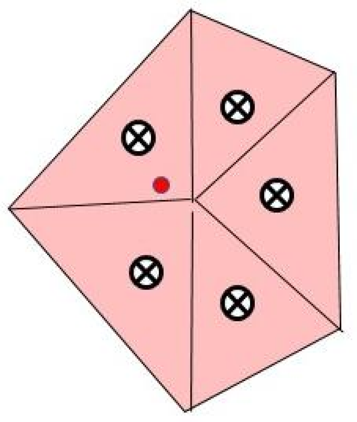
Figure 2: Once the polygon for a point is created, it is decomposed into triangles (2D) or tetrahedra (3D) for integration.

Note that the topological connection between the polytopes for each point is not computed, but only a unique polygon or polyhedron for each point independently. Figure 2a shows a cartoon of this process. The goal is to construct the Voronoi-like polygon for the central red point, which has a set of neighbor points it overlaps (in blue), and a non-zero kernel extent represented as the gray region. The starting polygon for this point is the bounding surface of this gray region, which is progressively clipped by planes half-way between the central red point and each of its neighbors. In the end all that is left is the central light red polygon, which is the unique volume closer to the red point than any of its neighbors. To facilitate simple integration quadratures, these polytopes for each point are further broken down into triangles (in 2D) and tetrahedra (in 3D). Fig. 2 shows this procedure for the polygon generated in Fig. 2, where the cross markers denote the centroid of each of the sub-triangles in the polygon. Note the centroid of the polygon does not necessarily coincide with the original point used to construct it.

3.2 Meshless integration quadrature

The set of integration quadratures over the base shapes represents a contiguous, non-overlapping quadrature that covers the domain. A Gauss-Legendre quadrature is used for integration of the line segments, while symmetric quadrature rules as described in Ref. [32] are used to integrate the triangles and tetrahedra. Appendix A presents information on how the integrals are transformed from physical to reference space.

At each integration point, all the functions whose support includes the integration point must be evaluated. The RK functions (Sec. 2.2) are expensive to evaluate relative to a standard SPH kernel and the evaluation of one such function depends on the values of all other functions at that point. As such, a large amount of computation can be saved by making the quadrature the outermost loop in the code, as shown in Alg. 1. For each quadrature point, all functions whose support includes the integration quadrature point are evaluated. Then these values are used to perform each integral.

It is worth comparing this approach with prior background integration methodologies, wherein a traditional background mesh (often some sort of orthogonal Cartesian grid aligned with the lab frame) is placed independently of the meshless points, even if the point locations inform characteristics of the background mesh. The approach in this section, using a Voronoi tessellation for the integration, produces an integration mesh whose properties are solely determined by the volume and relative positioning of the meshless points, which makes it invariant to rotation or translation. This integration does not meet the strictest of meshless criteria, in which no mesh is allowed [33], but does meet a looser criterion in that all information can be derived directly from the meshless points. The geometry of each point’s unique volume is constructed based solely on the positions of surrounding points without storing, evolving, or specifying anything except the the point positions and kernel extents.

3.3 Strong and weak forms for reproducing kernels

For the following sections, to simplify the notation, volume and surface integrals will be written as

$$\left\langle f,g\right\rangle=\int_{V}fgdV,$$ (30)

$$\left(f,g\right)=\int_{S}fgdS.$$ (31)

For many applications, such as hydrodynamics and diffusion, SPH and RK can be used to directly discretize the equations via collocation [8]. The equation, in this example

$$a^{\alpha}\partial_{x}^{\alpha}f+bf=0,$$ (32)

is first integrated by parts,

$$\left(U_{i},n^{\alpha}a^{\alpha}f\right)-\left\langle\partial_{x}^{\alpha}U_{i},a^{\alpha}f\right\rangle+\left\langle U_{i},bf\right\rangle=0,$$ (33)

(with $n$ denoting the surface normal), the surface term is discarded, and interpolants [Eq. (14)] and the delta function property [Eq. (9)] are used to simplify the equation to

$$-\sum_{j}V_{j}a_{j}^{\alpha}f_{j}\partial_{x_{i}}^{\alpha}U_{ji}+b_{i}f_{i}=0.$$ (34)

While this form of the equation has the advantage of simplicity, it depends on a one-point quadrature rule for the integration,

$$\int_{V}U_{i}f\left(x\right)\approx f_{i},$$ (35)

and generally throws away surface terms. Another option, and the one used in this paper, is to insert a basis function expansion,

$$f\left(x\right)=\sum_{j}V_{j}U_{j}g_{j}$$ (36)

(with coefficients $g_{j}$),

$$\sum_{j}V_{j}\left[\left(U_{i},n^{\alpha}a^{\alpha}U_{j}\right)-\left\langle\partial_{x}^{\alpha}U_{i},a^{\alpha}U_{j}\right\rangle+\left\langle U_{i},bU_{j}\right\rangle\right]g_{j}=0,$$ (37)

and perform the integrals directly using a quadrature like the one described in Sec. 3.2,

$$\left\langle\partial_{x}^{\alpha}U_{i},a^{\alpha}U_{j}\right\rangle\approx\sum_{k}w_{k}\partial_{x_{k}}^{\alpha}U_{ik}a_{k}^{\alpha}U_{jk},$$ (38)

where $w_{k}$ are the weights of a quadrature spanning the integration volume. For functions with compact support, this is the Meshless-Local Petrov-Galerkin (MLPG) method.

3.4 Meshless connectivity

Two types of connectivity are used in evaluating and storing the MLPG integrals. In a standard SPH code, the connectivity is the sets of points whose evaluation is nonzero at the center of the other, so points $i$ and $j$ are neighbors if the support of $W_{i}$ includes the point $x_{j}$ or vice versa, or

$$\chi\left(\eta\left(x_{i}-x_{j}\right)\right)\leq r,$$ (39)

where $r$ is the dimensionless support radius of the kernel. For MLPG, the connectivity (or sets of points for which the bilinear integrals are nonzero) is determined by whether points have overlapping support, so points $i$ and $j$ are neighbors if the support regions of $W_{i}$ and $W_{j}$ intersect. The overlap connectivity is a subset of the set of points for which

$$\chi\left(\eta\left(x_{i}-x_{j}\right)\right)\leq 2r.$$ (40)

To show this, suppose that there is a point $x_{k}$ that is in the support radius of $W_{i}$ and $W_{j}$. It follows from Eq. (39) and the triangle inequality in Euclidean space that $\chi\left(\eta\left(x_{i}-x_{j}\right)\right)\leq\chi\left(\eta\left(x_{i}-x_{k}\right)\right)+\chi\left(\eta\left(x_{k}-x_{j}\right)\right)\leq 2r$.

Standard SPH connectivity information can be used to both create the overlap connectivity and calculate which functions are nonzero at each integration point, which is similar to standard SPH connectivity. If the radius of the MLPG kernels is doubled (or the smoothing length altered to produce a similar effect), then by Eqs. (39) and (40), the standard SPH connectivity of the doubled-radius will include all overlap neighbors. As each cell produced by the Voronoi tessellation is completely contained within the support of its associated MLPG point, this same double-radius SPH connectivity for $i$ and $j$ will include all integration points in the cell $i$ for which the kernel $W_{j}$ is nonzero. This is why the same connectivity can be used for both the overlap of two kernels and the overlap of a kernel with a Voronoi cell associated with a kernel in Alg. 1.

4 Radiation transport

In this section, the radiation transport equation is introduced and discretized using MLPG with RK functions. Then, the iterative methods that are used for the solution of the discretized equation are described. Finally, the angular quadrature with selective refinement is introduced.

4.1 Discretization of the transport equation

The gray radiation transport equation, which is the transport equation integrated over all energies, is

$$\partial_{t}\psi+\Omega^{\alpha}\partial_{x}^{\alpha}\psi+\sigma_{t}\psi=\frac{1}{4\pi}\sigma_{s}\phi+q,$$ (41)

with the boundary condition

$$\psi=\psi^{b},\quad x\in\partial V,\ \Omega^{\alpha}n^{\alpha}>0,$$ (42)

and initial condition

$$\psi=\psi^{\text{init}},\quad t=0,$$

where $\Omega$ is the radiation propagation direction, $\psi$ is the angular flux, $\phi=\int_{4\pi}\psi d\Omega$ is the scalar flux, $\sigma_{s}$ is the scattering cross section, $\sigma_{a}$ is the absorption cross section, $\sigma_{t}=\sigma_{a}+\sigma_{s}$ is the total cross section, $q$ is a source that may include physics such as thermal emission, $\psi^{b}$ is the incoming flux at the boundary, $\psi^{\text{init}}$ is the initial angular flux, and $\partial V$ denotes the boundary of the domain. The discrete-ordinates approximation evaluates this equation at discrete angles that are ordinates of a quadrature over a unit sphere. Denoting these ordinates as $\Omega_{m}$ for the angular index $m$, integrals over the unit sphere become

$$\int_{4\pi}fd\Omega\approx\sum_{m}w_{m}f_{m},$$ (43)

where $w_{m}$ are the weights of the quadrature. The transport equation evaluated at the discrete ordinate $m$ becomes

$$\partial_{t}\psi_{m}+\Omega_{m}^{\alpha}\partial_{x}^{\alpha}\psi_{m}+\sigma_{t}\psi_{m}=\frac{1}{4\pi}\sigma_{s}\phi+q_{m},$$ (44)

with the scalar flux $\phi=\sum_{m}w_{m}\psi_{m}$. The backward Euler (or fully-implicit) method is used to discretize in time,

$$\frac{1}{c\Delta t}\psi_{m}+\Omega_{m}^{\alpha}\partial_{x}^{\alpha}\psi_{m}+\sigma_{t}\psi_{m}=\frac{1}{c\Delta t}\psi_{m}^{n-1}+\frac{1}{4\pi}\sigma_{s}\phi+q_{m},$$ (45)

where all variables are evaluated at time index $n$ except where noted otherwise as a superscript.

A standard Galerkin approach to transport would be to multiply the transport equation by $U_{i}$ and then integrate over the support of $U_{i}$. For streamline-upwind Petrov-Galerkin (SUPG) stabilization, the transport equation is instead multiplied by $U_{i}+\tau_{i}\Omega^{\alpha}\partial_{x}^{\alpha}U_{i}$, where $\tau$ is a proportionality constant with unit length that is chosen to be constant for each trial function. Performing this operation, the transport equation becomes

$$\frac{1}{c\Delta t}\left\langle U_{i},\psi_{m}\right\rangle+\frac{1}{c\Delta t}\tau_{i}\Omega_{m}^{\alpha}\left\langle\partial_{x}^{\alpha}U_{i},\psi_{m}\right\rangle+\left(U_{i},\Omega_{m}^{\alpha}n^{\alpha}\psi_{m}\right)_{\Omega^{\alpha}n^{\alpha}>0}-\Omega_{m}^{\alpha}\left\langle\partial_{x}^{\alpha}U_{i},\psi_{m}\right\rangle$$

$$\quad+\tau_{i}\Omega_{m}^{\alpha}\Omega_{m}^{\beta}\left\langle\partial_{x}^{\alpha}U_{i},\partial_{x}^{\beta}\psi_{m}\right\rangle+\left\langle U_{i},\sigma_{t}\psi_{m}\right\rangle+\tau_{i}\Omega_{m}^{\alpha}\left\langle\partial_{x}^{\alpha}U_{i},\sigma_{t}\psi_{m}\right\rangle$$

$$\qquad=\frac{1}{c\Delta t}\left\langle U_{i},\psi_{m}^{n-1}\right\rangle+\frac{1}{c\Delta t}\tau_{i}\Omega_{m}^{\alpha}\left\langle\partial_{x}^{\alpha}U_{i},\psi_{m}^{n-1}\right\rangle+\left(U_{i},\left|\Omega_{m}^{\alpha}n^{\alpha}\right|\psi_{m}^{b}\right)_{\Omega^{\alpha}n^{\alpha}<0}$$

$$\qquad\quad+\frac{1}{4\pi}\left\langle U_{i},\sigma_{s}\phi\right\rangle+\frac{1}{4\pi}\tau_{i}\Omega_{m}^{\alpha}\left\langle\partial_{x}^{\alpha}U_{i},\sigma_{s}\phi\right\rangle+\left\langle U_{i},q_{m}\right\rangle+\tau_{i}\Omega_{m}^{\alpha}\left\langle\partial_{x}^{\alpha}U_{i},q_{m}\right\rangle.$$ (46)

The surface integral term produced by integration by parts has been split into known (incoming) and unknown (outgoing) parts and the boundary condition [Eq. (42)] has been applied. Inserting a basis function expansion for the scalar and angular flux [as in Eq. (36)],

$$\phi=\sum_{j}V_{j}U_{j}\Phi_{j},$$ (47a)

$$\psi=\sum_{j}V_{j}U_{j}\Psi_{j},$$ (47b)

the equation becomes

$$\sum_{j}V_{j}\left[\frac{1}{c\Delta t}\left\langle U_{i},U_{j}\right\rangle+\frac{1}{c\Delta t}\tau_{i}\Omega_{m}^{\alpha}\left\langle\partial_{x}^{\alpha}U_{i},U_{j}\right\rangle+\left(U_{i},\Omega_{m}^{\alpha}n^{\alpha}U_{j}\right)_{\Omega^{\alpha}n^{\alpha}>0}-\Omega_{m}^{\alpha}\left\langle\partial_{x}^{\alpha}U_{i},U_{j}\right\rangle\right.$$

$$\quad\left.+\tau_{i}\Omega_{m}^{\alpha}\Omega_{m}^{\beta}\left\langle\partial_{x}^{\alpha}U_{i},\partial_{x}^{\beta}U_{j}\right\rangle+\left\langle U_{i},\sigma_{t}U_{j}\right\rangle+\tau_{i}\Omega_{m}^{\alpha}\left\langle\partial_{x}^{\alpha}U_{i},\sigma_{t}U_{j}\right\rangle\right]\Psi_{m,j}$$

$$\qquad=\sum_{j}V_{j}\left[\frac{1}{c\Delta t}\left\langle U_{i},U_{j}\right\rangle+\frac{1}{c\Delta t}\tau_{i}\Omega_{m}^{\alpha}\left\langle\partial_{x}^{\alpha}U_{i},U_{j}\right\rangle\right]\Psi_{m,j}^{n-1}+\left(U_{i},\left|\Omega_{m}^{\alpha}n^{\alpha}\right|\psi_{m}^{b}\right)_{\Omega^{\alpha}n^{\alpha}<0}$$

$$\qquad\quad+\frac{1}{4\pi}\sum_{j}V_{j}\left[\left\langle U_{i},\sigma_{s}U_{j}\right\rangle+\tau_{i}\Omega_{m}^{\alpha}\left\langle\partial_{x}^{\alpha}U_{i},\sigma_{s}U_{j}\right\rangle\right]\Phi_{j}+\left\langle U_{i},q_{m}\right\rangle+\tau_{i}\Omega_{m}^{\alpha}\left\langle\partial_{x}^{\alpha}U_{i},q_{m}\right\rangle.$$ (48)

Note that, in general, $\Phi_{i}\neq\phi_{i}$ and $\Psi_{i}\neq\psi_{i}$. Once Eq. (48) is solved for $\Phi$ and $\Psi$, the solution at each point must be recovered using Eqs. (47).

The effect of the SUPG stabilization is to reduce oscillations and make the system of equations easier to solve iteratively while not affecting global particle balance [18]. For the results in Sec. 5, the stabilization parameter is set to be

$$\tau_{i}=\frac{h_{i}}{k},$$

where $k$ is approximately the number of points across the kernel radius. This results in a $\tau_{i}$ that is approximately equal to the spacing between the points.

Because RK permits interpolation, the initial condition can be set using initial values of the angular flux instead of needing to interpolate coefficients, or $\Psi_{i}\bigg{|}_{t=0}=\psi^{\text{init}}\bigg{|}_{x=x_{i}}$. This is what is done for the results in Sec. 5.

4.2 Methods for solution of the transport equation

The transport equation can be written in operator form as

$$\mathcal{L}\Psi=\mathcal{T}\Psi^{n-1}+\mathcal{M}\mathcal{S}\Phi+r,$$ (49)

or in terms of $\Phi$ as

$$\left(\mathcal{I}-\mathcal{D}\mathcal{L}^{-1}\mathcal{M}\mathcal{S}\right)\Phi=\mathcal{D}\mathcal{L}^{-1}\left(\mathcal{T}\Psi^{n-1}+r\right),$$ (50)

with the operators defined as

$$\left(\mathcal{L}\Psi\right)_{m,i}= \sum_{j}V_{j}\left[\frac{1}{c\Delta t}\left\langle U_{i},U_{j}\right\rangle+\frac{1}{c\Delta t}\tau_{i}\Omega_{m}^{\alpha}\left\langle\partial_{x}^{\alpha}U_{i},U_{j}\right\rangle+\left(U_{i},\Omega_{m}^{\alpha}n^{\alpha}U_{j}\right)_{\Omega^{\alpha}n^{\alpha}>0}-\Omega_{m}^{\alpha}\left\langle\partial_{x}^{\alpha}U_{i},U_{j}\right\rangle\right.$$

$$\quad\left.+\tau_{i}\Omega_{m}^{\alpha}\Omega_{m}^{\beta}\left\langle\partial_{x}^{\alpha}U_{i},\partial_{x}^{\beta}U_{j}\right\rangle+\left\langle U_{i},\sigma_{t}U_{j}\right\rangle+\tau_{i}\Omega_{m}^{\alpha}\left\langle\partial_{x}^{\alpha}U_{i},\sigma_{t}U_{j}\right\rangle\right]\Psi_{m,j},$$ (51)

$$\left(\mathcal{T}\Psi^{n-1}\right)_{m,i} =\sum_{j}V_{j}\left[\frac{1}{c\Delta t}\left\langle U_{i},U_{j}\right\rangle+\frac{1}{c\Delta t}\tau_{i}\Omega_{m}^{\alpha}\left\langle\partial_{x}^{\alpha}U_{i},U_{j}\right\rangle\right]\Psi_{m,j}^{n-1},$$ (52)

$$\left(\mathcal{M}\mathcal{S}\Phi\right)_{i,m} =\frac{1}{4\pi}\sum_{j}V_{j}\left[\left\langle U_{i},\sigma_{s}U_{j}\right\rangle+\tau_{i}\Omega_{m}^{\alpha}\left\langle\partial_{x}^{\alpha}U_{i},\sigma_{s}U_{j}\right\rangle\right]\Phi_{j},$$ (53)

$$\left(\mathcal{D}\Psi\right)_{i} =\sum_{m}w_{m}\Psi_{m,i},$$ (54)

$$\left(r\right)_{i,m} =\left(U_{i},\left|\Omega_{m}^{\alpha}n^{\alpha}\right|\psi_{m}^{b}\right)_{\Omega^{\alpha}n^{\alpha}<0}+\left\langle U_{i},q_{m}\right\rangle+\tau_{i}\Omega_{m}^{\alpha}\left\langle\partial_{x}^{\alpha}U_{i},q_{m}\right\rangle.$$ (55)

Note that using this notation, $\Phi=\mathcal{D}\Psi$. The notation $\mathcal{L}^{-1}$ denotes the linear inverse of the $\mathcal{L}$ operator, which is block diagonal in angle. With the first-flight source defined as

$$b_{\psi}=\mathcal{L}^{-1}\left(\mathcal{T}\Psi^{n-1}+r\right),$$ (56)

$$b_{\phi}=\mathcal{D}b_{\psi},$$ (57)

the equation can be simplified to

$$\left(\mathcal{I}-\mathcal{D}\mathcal{L}^{-1}\mathcal{M}\mathcal{S}\right)\Phi=b_{\phi}.$$ (58)

Equation (58) can be solved directly using a matrix-free linear solver such as GMRES or iteratively using a method such as fixed point iteration. Once the scattering source is converged, the angular flux is recovered for use in the next time step by performing an additional solve using the converged scalar flux,

$$\Psi=\mathcal{L}^{-1}\mathcal{M}\mathcal{S}\Phi+b_{\psi}.$$ (59)

For the results in Sec. 5, the $\mathcal{L}^{-1}$ operation is performed using two packages from Trilinos [34], the Belos package for GMRES and the Ifpack2 package for the ILUT preconditioner. The ILUT factorizations for each angle are precomputed at the start of the time step and reused to minimize computation. The iterations to converge the scattering source [the solution of Eq. (58)] are also performed using GMRES from Belos without a preconditioner. For a discussion on preconditioners for the scattering iterations, see Sec. 6.

4.3 Refinement of the angular quadrature

For the problems in Sec. 5, the Gauss-Legendre quadrature is used in 1D, while the LDFE (linear discontinuous finite element) quadrature [35] is used in 2D and 3D. The LDFE quadrature is hierarchal, meaning that each octant of the unit sphere can be further subdivided into four ordinates, which can themselves be subdivided and so on. This can be used to produce a high density of angular ordinates in chosen directions object to prevent ray effects, which as shown in Sec. 5.4. Given a goal quadrature, the refined angular discretization keeps all ordinates from the goal quadrature that hit the object and combines the ordinates that do not hit the object inasmuch as is possible (Alg. 2). This significantly reduces the number of angles needed for a given number of rays from a small source to hit a distant object.

5 Results

In this section, five problems are considered to test the discretization described in Sec. 4 with the integration in Sec. 3. The first two problems use the method of manufactured solutions. The third problem considers a purely absorbing medium, while the fourth problem considers a purely scattering medium. The final problem shows a possible application of the code to simulate an asteroid absorbing a large quantity of radiation from a distant source. All the problems use a kernel sampling radius of 4 neighbors (i.e., the equivalent smoothing scale is 4 times the local particle spacing) and an RK order of one, as described in Sec. 3, except for the purely absorbing problem, which also explores other combinations of RK order and neighbors. Note that for uniformly spaced points, a sampling radius of 4 neighbors implies a total number of overlap neighbors for each point of 8 (1D), 50 (2D), and 268 (3D).

The first two sections use the relative error as a measure for convergence. This is defined as

$$\epsilon_{rel}=\dfrac{\sum_{i}\left|\phi_{i}^{\text{numeric}}-\phi_{i}^{\text{analytic}}\right|}{\sum_{i}\phi_{i}^{\text{analytic}}}$$ (60)

for the numeric and analytic scalar fluxes at the MLPG centers $i$.

5.1 Manufactured problems

The method of manufactured solutions works by selecting a solution for $\psi$, solving for a source $q$ by inserting this solution into the continuous transport equation [Eq. (41)], assigning the boundary source $\psi_{b}$ to be equal to the solution, and then calculating a numerical solution using the discretized transport equation [Eq. (48)] for comparison to the original solution.

The spatial and time convergence of the manufactured problems is considered in 1D, 2D, and 3D. In 1D, due to the low cost of integration and because the integration cells are not subdivided, the integration is performed using a 64-point Gauss-Legendre quadrature. In 2D, the integration of the subcell triangles is performed using a tenth-order symmetric quadrature with 25 points, while in 3D, the integration of the surface triangles and the subcell tetrahedra is performed using a third-order symmetric quadrature with 8 points. For more information on the integration quadratures, see Sec. 3.

The spatially-dependent results are run for several cases between $8^{d}$ and $128^{d}$ points (for the dimension $d$) without time dependence. For the time-dependent case, the simulation is run until $t=1$ with time steps between 0.001 and 1.0 and $64^{d}$ points. The minimum time step is increased to 0.01 in 2D and 0.1 in 3D. In each case the points are laid down in a spatially uniform lattice configuration. For the non-uniform cases, the point positions are randomly perturbed by up to 0.2 times the point distance in each dimension, or $x^{\alpha}=x^{\alpha}\pm\Delta x^{\alpha}\gamma^{\alpha}$, where $-0.2\leq\gamma^{\alpha}\leq 0.2$ is randomly generated for each point and dimension independently and $\Delta x^{\alpha}$ is the point spacing for the given dimension.

5.1.1 Sinusoidal manufactured problem

The first manufactured solution,

$$\psi_{\text{sinusoidal}}=1+\frac{1}{2\pi}\prod_{\alpha}\cos\left(\pi\left(x^{\alpha}+t\right)\right),$$ (61)

is designed to test convergence of the discretized transport equation [Eq. (48)]. The solution is chosen such that the manufactured source never becomes negative, which would be unphysical. To ensure that the integration of the cross sections [Sec. 3] works correctly, the scattering and absorption opacities are also chosen to have sinusoidal values that are out of phase with the solution and one another,

$$\sigma_{a}=1+\frac{2}{3}\prod_{\alpha}\cos\left(3x^{\alpha}\right),$$ (62)

$$\sigma_{s}=1+\frac{3}{4}\prod_{\alpha}\sin\left(2x^{\alpha}\right).$$ (63)

The domain is $-1\leq x^{\alpha}\leq 1$. For the steady-state case, the manufactured solution is fixed at $t=0$.

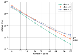
(a) Manufactured sinusoidal solution, uniform.

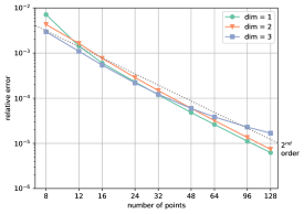
(b) Manufactured wave solution, uniform.

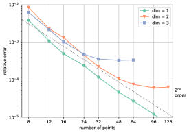
(c) Manufactured sinusoidal solution, perturbed.

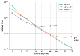
(d) Manufactured wave solution, perturbed.

Figure 3: Spatial convergence of the manufactured solutions at steady-state in 1D, 2D, and 3D, with the dotted line indicating second-order convergence. For two of the cases, the point positions are randomly perturbed. The perturbation may cause insufficient support for the RK functions or lower integration accuracy, leading to a lack of convergence.

The spatial convergence results in Fig. 3a indicate second-order convergence in 1D, 2D, and 3D, as expected for linear RK corrections. The 3D results eventually plateau around 96 points. It is likely that the difference between the numeric and analytic solution is reaching the accuracy limit of the third-order quadrature in 3D, which appears to reduce the convergence order to first-order. The inclusion of spatially-dependent cross sections does not appear to hinder convergence.

When the point positions are randomly perturbed (Fig. 3c), the convergence rate stays the same, with a caveat. The algorithm for calculating kernel extents is designed for hydrodynamics and requires that the average level of support is above a certain threshold, not the support for each point. It is possible that in 2D and 3D, the solution reaches the accuracy of the poorly-supported RK calculation and stops converging for certain points. Before this occurs, the convergence is second-order. When the calculation is run with a higher kernel extent (not pictured), the quantitative behavior is similar but the error levels off at a lower value. The other difference between dimensions is the integration quadrature, which is coarser and less accurate between dimensions. This could be contributing to the leveling off of the error.

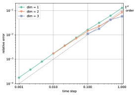
(a) Manufactured sinusoidal solution.

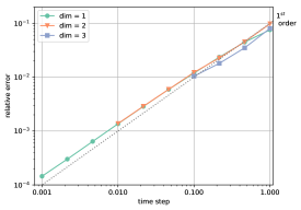
(b) Manufactured wave solution.

Figure 4: Temporal convergence of the manufactured solutions in 1D, 2D, and 3D, with the dotted line indicating first-order convergence.

The temporal convergence rate is first-order (Fig. 4a), as expected from the backward Euler time discretization. The 2D and 3D results have similar or lower error than the 1D results for a similar number of points, which may be due to the higher level of connectivity in 2D and 3D. For this problem, the time discretization error even with the smallest time step considered (0.001) is similar to the spatial discretization error with $32^{d}$ points. It is expected that to increase the accuracy of a time-dependent simulation at the point where the temporal and spatial discretization errors are similar, the time step would need to be decreased as the distance between points squared.

5.1.2 Outgoing wave manufactured problem

The second manufactured problem represents a wave traveling from the origin outward,

$$\psi_{\text{wave}}=1+\frac{1}{t^{2}+6}\exp\left(-10\left[\left|x\right|-t\right]^{2}\right),$$

with constant opacities of $\sigma_{a}=0.5$ and $\sigma_{s}=2.0$ and a domain of $-1\leq x^{\alpha}\leq 1$. For the steady-state case, the manufactured solution is fixed at $t=0.5$.

As in the sinusoidal case, the spatial convergence is second-order (Fig. 3b) and the temporal convergence is first-order (Fig. 4b). The magnitude of the error is similar in the wave and the sinusoidal case, and just as in the sinusoidal case, the error in 3D plateaus on the spatial convergence plot, probably due to the integration error. The perturbed version of the steady-state problem (Fig. 3d) has similar behavior to the sinusoidal case described above, with second-order convergence until reaching issues with either RK kernel support or integration.

5.2 Purely absorbing problem

One challenge in transport is handling highly absorptive regions without incurring negative fluxes. In this problem, a single ray with $\Omega=\left\{1,0,0\right\}$ is incident on a purely absorbing slab with a domain $0\leq x\leq 1$, which is modeled in 1D. First, a constant cross section of $\sigma_{a}=5$ is considered with a variable number of points between 8 and 64. Then, the number of points is held constant at $32$ and the cross section is varied between $1$ and $64$. The points are again placed uniformly.

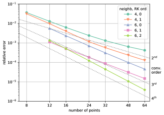
Figure 5: Relative error of the numeric solution to the purely absorbing problem as the number of points is increased for various combinations of the number of neighbors and RK correction order, with the dotted lines indicating second, third, and fourth-order convergence.

Convergence results are shown in Fig. 5 for a few cases of the RK order and the number of neighbors, which is the number of other points across a kernel radius for the base connectivity used to create the overlap connectivity. The number of neighbors for the reduced-radius kernels should be at least one higher than the RK order to prevent the system in Eq. (24) from being singular, which means that the number of neighbors for the original kernels (which is the number reported here) should be two times the RK order plus one. For zeroth-order RK corrections, the solution converges with approximately second-order accuracy. For first-order corrections, the solution converges with approximately second-order accuracy for 4 neighbors and between second and third order for 6 neighbors. With second-order corrections and 6 neighbors, the convergence order is between third and fourth. In general, for a smooth solution, the expected convergence order is one greater than the RK order.

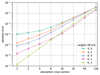
Figure 6: Absolute error of the numeric solution to the purely absorbing problem for various combinations of the number of neighbors, RK correction order, and absorption cross section.

Results for the case with a constant number of points and a changing cross section are shown in Fig. 6. For this problem, in which the primary gradient is at the edge of the problem with the lowest point density, the MLPG approach requires around one point per mean free path of the material to avoid negativities, which is reflected in the results. The solution begins to exhibit negativities at $\sigma_{a}=32$ for the case with 6 neighbors, while for 4 neighbors, the negativities show up for $\sigma_{a}=64$ and above. Note that the error is an absolute error, since the normalization would otherwise skew the results. As in the convergence study, an increasing number of neighbors and RK order decrease the solution error.

Based on these results, it may be tempting to use kernels with large radii and high RK order for other problems to increase solution accuracy. One issue with this is computational cost, which increases significantly in 2D and 3D as the function radii increase. Since the RK order is limited for kernels with small radii, this also limits the RK order. For instance, in 3D, the number of neighbors increases as $r^{3}$, where $r$ is the kernel radius, so moving from 4 neighbors across the kernel radius to 6 will more than triple the cost. This also increases the difficulty of solving the transport system (the $\mathcal{L}^{-1}$ operation). Another issue is negativities, which are present for all the 32-point simulations with 6 neighbors but not for any 32-point simulations with 4 neighbors. These negativities can become amplified in time-dependent problems, where a negative absorption becomes an unphysical source of particles. For more discussion on negative fluxes, see Sec. 6.

5.3 Crooked pipe problem

This problem is described in Ref. [36] as a test of diffusion synthetic acceleration (DSA). Results for the MLPG code with the Krylov iteration as described in Sec. 4.2 are compared to those from a code based on the discontinuous finite element method (DFEM) with acceleration based on a variable Eddington factor (VEF), as described in Ref. [37].

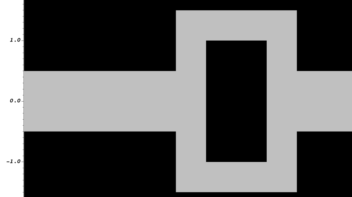
Figure 7: Geometry of the cooked pipe problem. The scattering opacities are $\sigma_{s}=200$ in the black region and $\sigma_{s}=0.2$ in the gray region.

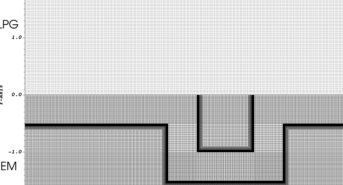
Figure 8: The MLPG points (top) and DFEM mesh (bottom) for the crooked pipe problem, at 1/4 resolution for visibility. Note that the DFEM mesh has additional resolution near the thin-thick boundary.

The geometry for the problem is shown in Fig. 7, with $\sigma_{s}=200$ in the wall and $\sigma_{s}=0.2$ in the pipe. The absorption cross section is zero in both regions. The relatively coarse angular discretization with 16 ordinates is identical between the MLPG and DFEM codes. The MLPG results have a spatial discretization with 716,800 equally-spaced points (or 160 by 160 points per unit area), while the DFEM results are calculated on a mesh with 1,335,296 elements, with a higher density of elements placed near the pipe-wall boundary. The MLPG points and DFEM mesh at quarter resolution (or 16 times fewer points) is shown in Fig. 8. The units for the problem are set such that the speed of light is $c=1$. The problem is run until $t=20$ with a fixed time step of $\Delta t=0.1$.

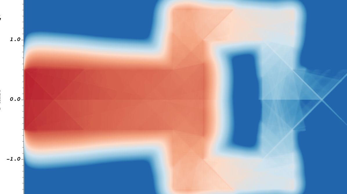
(a) $t=10$

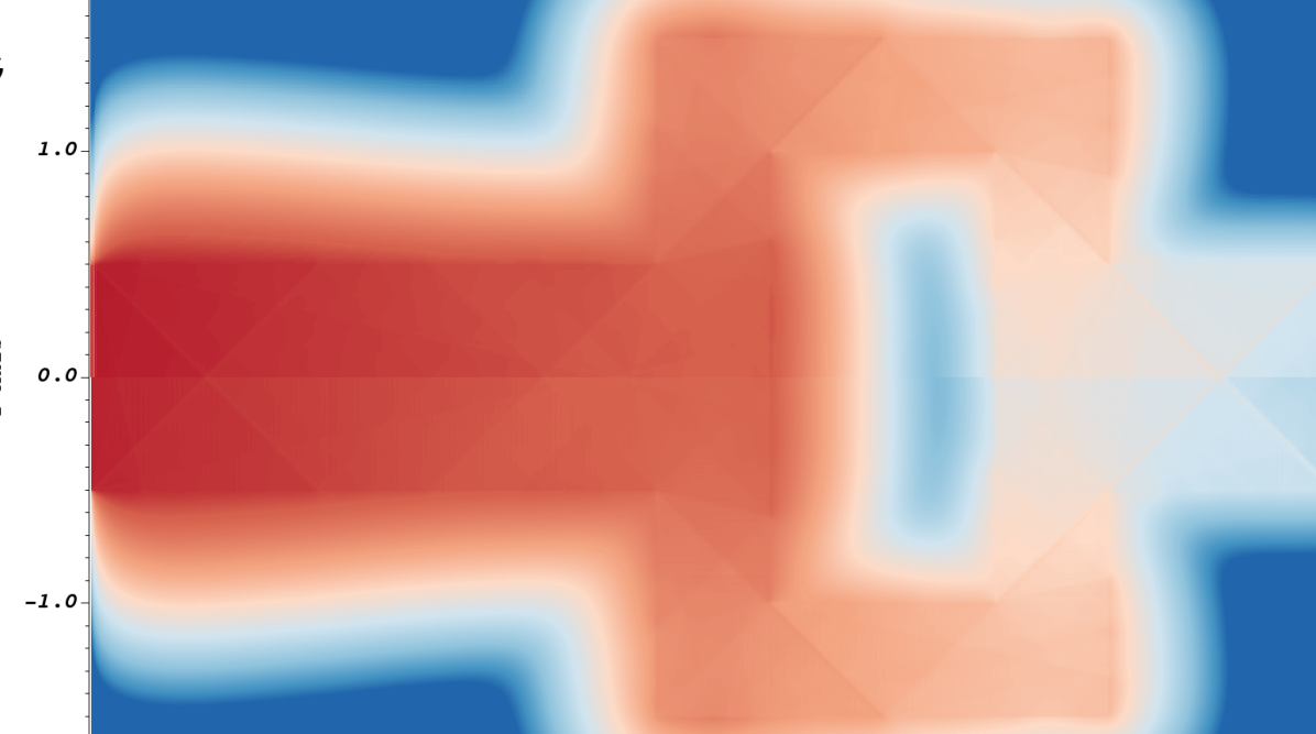
(b) $t=20$

Figure 9: The scalar flux for the MLPG (top) and DFEM (bottom) solutions to the crooked pipe problem at two times.

A comparison of the crooked pipe results at $t=10$ and $t=20$ is shown in Fig. 9. The propagation speed of the radiation appears is nearly identical between the two codes. For the $t=10$ plot, the radiation would have traveled 10 unit distance at most in the 10 unit time (since $c=1$). The minimum path the radiation could take to reach the plane at $x=2$ from the source at $x=-3.5$ is $6.5$ unit distance. Depending on the direction, the actual distance the radiation would need to travel to reach the plane $x=2$ would be at between 7 and 12 unit distance. The strongest visible ray is at $\Omega^{\alpha}=1/\sqrt{3}$, which would have reached $x=2$ at $t=9.5$ if scattering and corners were neglected. As the radiation appears to have just reached $x=2$ at $t=10$, the calculated time of arrival is close to the distance the radiation would have traveled in that time.

The results show significant ray effects, but because the two codes use the same angular quadrature, the effects appear to be the same. Before reaching the crooked part of the problem, there are no significant differences visible between the two solutions. After the radiation has gone around the obstacle, the MLPG solution is higher in magnitude, which is visible in the $t=10$ plot near the right edge of the obstacle or in the $t=20$ plot at the exiting surface of the pipe. Part of this could be due to the higher resolution along the pipe-wall interface in the DFEM simulation, which could affect the scattering rate at the interface. The contours of the solution near the interfaces also line up very closely, except at the wall edge at $x=0.5$, where the MLPG solution reaches a further through the wall, which could again be due to the lower resolution near the interface.

As mentioned before, this problem has been used as a test of DSA. The Krylov solution procedure [for the solution of the MLPG system in Eq. (58)] works for this case without preconditioning, with an average of 64 iterations to converge. As the ILUT factorization of the matrices representing the $\mathcal{L}^{-1}$ operation is performed once and stored, this doesn’t increase the total simulation time by nearly 64 times more than a single iteration, as the factorization is a far larger cost than a single solve. Within each scattering iteration, the transport GMRES solver converges to a tolerance of $10^{-15}$ in 55 iterations on average. The DFEM solution, however, required only one transport solve and two VEF solves per time step, which if applied to the MLPG solution could open up more cost-effective methods for solving for the scattering source.

For general reference, the RK transport code takes 15,943 seconds, or 79 seconds per time step, to run the crooked pipe problem with 16 ordinates and 716,800 points on 288 processors, which equates to 2,488 points or 39,808 unknowns per processor on average. This includes the time for integration, computation of the ILUT preconditioners for all 16 directions, and convergence of the solution and scattering source. With an effective preconditioner and possibly avoiding ILUT decompositions, the solve time would decrease significantly. The need for appropriate preconditioning is discussed further in Sec. 6.

5.4 Asteroid problem

One motivation for combining radiation transport with a smoothed particle hydrodynamics code is for a planetary defense application: the deflection of an asteroid due to radiation from a standoff nuclear burst. In this scenario, the absorbed radiation energy ablates the surface of the asteroid, causing material to blow off and alter the orbit of the asteroid via momentum conservation. This problem is a simplified version of that scenario, a spherical rock “asteroid” that absorbs radiation from a distant point source in 2D. This problem is similar to the purely-absorbing version of Kobayashi benchmarks [38], which also have features that are difficult to angularly resolve and a small source emitting particles into a void. The asteroid has an absorption cross section of $\sigma_{a}=10.0$, while the medium surrounding the asteroid has an absorption cross section of $\sigma_{a}=0.001$. Neither material includes scattering. The asteroid has a radius of 35 and is centered at the origin. The point source is located a distance of 70 away from the surface of the asteroid. The asteroid can be modeled by a shell, since almost all of the radiation is absorbed at the surface of the asteroid.

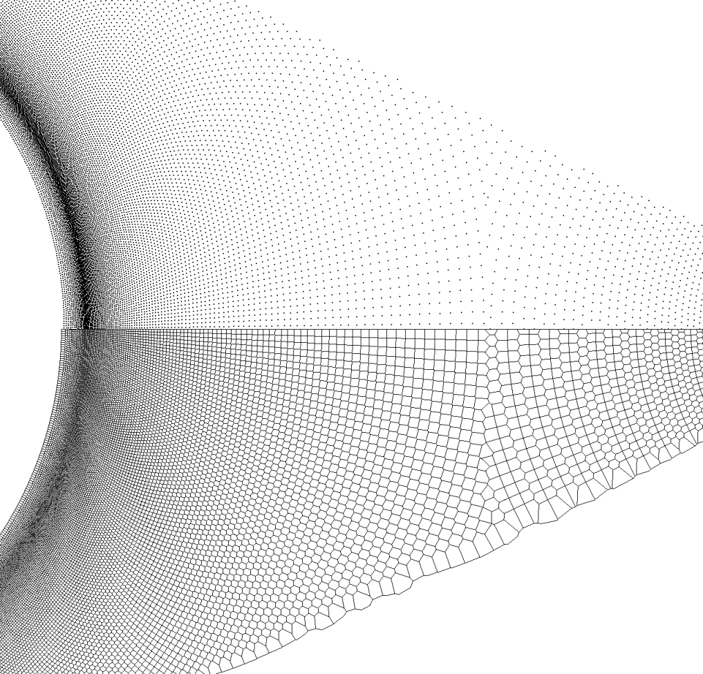
Figure 10: The solution points (top) and integration mesh (bottom) for the asteroid problem. Note that the resolution of the integration mesh mirrors that of the kernels. The integration cells are further subdivided into triangles for integration.

The shell of the asteroid is set to be 20 mean free paths thick. The distance between points is set to be 0.2 at the inside of the shell of the asteroid, 0.1 at the outside of the shell, 1.0 halfway between the source and the asteroid, and 0.1 near the source. The initial angular quadrature of 4,096 ordinates is refined as described in Sec. 4.3 down to 550 ordinates, of which 480 hit the asteroid. The problem is run with a single time step large enough for the radiation to propagate throughout the domain. Afterward, the numeric solution is compared to the analytic solution, which is derived in App. B. The solution points and integration mesh for this problem are shown in Fig. 10. Note that the integration mesh is further broken down into triangles for use with standard quadratures (Sec. 3).

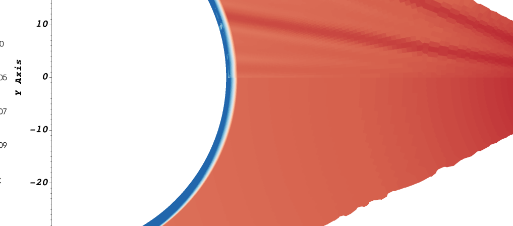
Figure 11: The numeric (top) and analytic (bottom) scalar flux solution to the asteroid problem. The low resolution for rays that miss the asteroid is by design. Note the ray effects where the radiation propagation direction is parallel to the surface of the asteroid.

The analytic and numeric solutions to the asteroid problem are shown in Fig. 11. The most obvious difference at first glance is the large areas at the top of the numeric solution where the solution is close to zero. These are areas where, by design, the angular refinement has not put a sufficient number of angles to resolve the solution. These should not affect the solution at the asteroid, since there, the solution should be sufficiently resolved in the angular domain. While there are 480 rays that hit the asteroid from the point source, the radiation is still not angularly uniform in the region that is resolved, as can be seen by the more intense ray that hits the asteroid around the point $\left\{11,33\right\}$.

Near the $y=0$ plane, where there is approximately one point per mean free path in the direction the solution is changing, the contours of the analytic and numeric solutions line up very well, with the exception of the aforementioned oscillations. This agrees with the purely absorbing results (Sec. 5.2), in which the solutions with around one point per mean free path showed higher accuracy and few oscillations compared to those with more than one point per mean free path.

There are two connected difficulties in this problem, which are ray effects and negativities. Oscillations can be seen toward the inner surface of the asteroid at all positions, but the oscillations are by far the worst where the radiation is traveling nearly parallel to the surface of the asteroid. At these points, the solution will change from the vacuum solution just outside of the surface to nearly zero inside of the surface. This causes oscillations that lead to negativities. The SUPG stabilization does a good job of handling the oscillations that may develop in the direction of radiation propagation (near the $y=0$ plane), but more consideration is needed to prevent the oscillations that develop perpendicular to the radiation propagation direction or when the solution changes discontinuously.

This problem is designed to stress the code and show opportunities for future work. If the results needed to be accurate, the source could be analytically calculated just before it hits the asteroid and inserted as a boundary source there, which would reduce much of the need for a refined and specialized quadrature. The negatives, however, would persist, which is something that would need to be addressed before this calculation would work well in a time-dependent or thermal radiative transfer scenario, as discussed in Sec. 6.

6 Conclusions and future work

The MLPG discretization in this paper simplifies the process running a problem with meshless transport. The fully-implicit time differencing is stable for large time steps. The SUPG stabilization works to prevent oscillations and increase the efficiency of inverting the transport matrix. The integration with a Voronoi diagram is robust and follows the resolution of the meshless points without user input. The SUPG stabilization and Voronoi integration add complexity to the code, which could be a barrier to entry, but reduces the need for specialized solvers or repeated adjustments of a background mesh.

The RK functions used in the discretization permit higher-than-second-order convergence, but practically, the radii of the kernels should often be minimized to reduce negativities and computation cost, which constrains the RK order. With the fully-implicit time discretization and first-order RK corrections, the results are consistent with second-order convergence in space and first-order convergence in time. For a purely absorbing problem with an incoming source, higher-order convergence is achieved in space with second-order RK corrections and larger kernel radii. The two manufactured solutions show the capability to represent spatially-dependent cross sections and converge in 1D, 2D, and 3D.

There are at least three issues that remain to be resolved. The first is negativities. In the purely-absorbing problem, around one point is needed per mean free path to avoid negativities. In the asteroid problem, negativities are difficult to avoid due to ray effects, as the SUPG stabilization applies numerical diffusion only in the direction of radiation propagation. A negative flux fixup method such as the zero-and-rescale approach [39] may work for meshless transport, but care would need to be taken to rescale a quantity that should always be positive and not the expansion coefficients. While this could inhibit the effects of oscillations on time-dependent problems and perhaps keep them from growing, it would be much more difficult to remove oscillations entirely.

The second issue is preconditioning. In the crooked pipe problem, the solution converged when using only GMRES to converge the scattering source and agreed well with a DFEM solution, but this required many iterations to achieve. Combining the Krylov solve with a method such as DSA [40] could significantly reduce the number of iterations needed to converge the scattering source. The MLPG transport equation without SUPG should have the diffusion limit, similar to a high-order DFEM discretization [41], but it is not apparent whether the same is true with SUPG. The process of deriving DSA for the SUPG system should give information on whether it has the diffusion limit and if not, what changes may be made to the discretized system to ensure it has the diffusion limit.

The third issue is ensuring proper support for the RK kernels. As shown in the manufactured problems, randomly perturbing the point positions can lead to a limit on convergence. Ensuring that every point has the needed support individually through a more robust calculation may resolve these issues.

The current meshless discretization works well for problems in which the solution does not go negative. Once a negative flux fixup treatment is applied, the addition of additional physics to the transport discretization such as thermal radiative transfer and radiation hydrodynamics would be more achievable. In a radiation hydrodynamics simulation, where the meshless topology is constantly changing, the consistently discretized transport with a Voronoi integration approach eliminates mapping to and from a mesh for radiation transport and is far cheaper than placing a non partition-of-unity quadrature for each kernel.

Appendix A Integral transformations

This section describes transformations of volume and surface integrals from a reference element (a line segment in 1D, a triangle in 2D, and a tetrahedron in 3D) to an element in physical space. For information on the meshless integration methods that produce these elements, see Sec. 3.

A.1 Volume integrals

The integrals described in Sec. 3 need to be mapped from reference space $R$ to physical space $V$,

$$\int_{V}f\left(x\right)dV=\int_{R}f\left(x\left(\xi\right)\right)\left|J\right|dR,$$ (64)

where $x$ and $\xi$ are the coordinates in physical and reference space, respectively, and $J$ is the Jacobian determinant of the transformation,

$$J^{\alpha\beta}=\frac{\partial x^{\beta}}{\partial\xi^{\alpha}}.$$ (65)

In discrete form, the quadrature is mapped using

$$\int_{V}f\left(x\right)dV\approx\sum_{m}w_{m}\left|J_{m}\right|f\left(x\left(\xi_{m}\right)\right),$$ (66)

where $w_{m}$ are the weights of the reference quadrature, which effectively converts the ordinates to $x\left(\xi_{m}\right)$ and the weights to $w_{m}\left|J_{m}\right|$ for the integration.

The line quadrature is assumed to have the bounds $-1\leq\xi\leq 1$, while the triangular and tetrahedral quadratures have the bounds $0\leq 1^{\alpha}\xi^{\alpha}\leq 1$, where $1^{\alpha}$ represents a vector of ones. For a line with points $p_{0}$ and $p_{1}$ in physical space, the mapping to reference space is

$$x\left(\xi\right)=p_{0}+\left(p_{1}-p_{0}\right)\frac{\left(\xi+1\right)}{2}.$$ (67)

For a triangle with points $p_{0}$, $p_{1}$, and $p_{2}$ or a tetrahedron with an additional point $p_{3}$, the mapping is

$$x\left(\xi\right)=p_{0}+\left(p_{\alpha}-p_{0}\right)\xi^{\alpha}.$$ (68)

A.2 Surface integrals

For surface integrals, the mapping is between reference space $T$ with coordinates $\xi$ and physical space $S$ with coordinates $x$,

$$\int_{S}f\left(x\right)dS=\int_{T}f\left(x\left(\xi\right)\right)KdT,$$ (69)

where $K$ is a differential surface element. For a triangle mapped from a 2D reference element to a 3D surface element, this term is

$$K=\left|\partial_{\xi_{1}}x\times\partial_{\xi_{2}}x\right|,$$ (70)

while for a line mapped from a 1D to a 2D line element, the differential element is

$$K=\left|\partial_{\xi}x\right|,$$ (71)

with the line and surface integrals mapped as in Eqs. (67) and (68), with the exception that the $p$ vectors have one more element than the $\xi$ ones (e.g. in 3D, the $p$ vectors have three elements, while the $\xi$, which is a surface parameterization, has only two). In discrete form, the surface integrals are

$$\int_{S}f\left(x\right)dS\approx\sum_{m}w_{m}K_{m}f_{m}.$$ (72)

Appendix B Analytic solution to asteroid problem

In this section, the analytic solution for the asteroid problem described in Sec. 5.4 is derived. In 2D, the “asteroid” is actually an infinite cylinder and the “point source” is a line source. The transport equation for this problem can be written in cylindrical geometry as

$$\mu\frac{1}{r}\partial_{r}\left(r\psi\right)+\sigma_{a}\psi=\delta\left(r\right),$$ (73)

where $r$ is the distance from the point source and $\mu$ is the cosine of the angle between the x-y plane and the radiation propagation direction. The cross section is

$$\sigma_{a}=\begin{cases}\sigma_{a,\text{background}},&r<d_{\text{asteroid}},\\ \sigma_{a,\text{asteroid}},&\text{otherwise},\end{cases}$$ (74)

where $d_{\text{asteroid}}$ is the distance from the source to the asteroid for a given evaluation point. The solution to this equation is

$$\psi=\frac{1}{r}\exp\left(-\frac{1}{\mu}\omega\right),$$ (75)

where

$$\omega=\int_{0}^{r}\sigma_{a}dr^{\prime},$$ (76)

which can be calculated using only the distance travelled in each of the asteroid and the background along with their respective cross sections. Integrating this equation over all forward angles, $0\leq\mu\leq 1$ (which is also the only set of angles for which the solution is nonzero), the scalar flux solution is

$$\phi=\frac{1}{r}\left[\exp\left(-\omega\right)-\omega\int_{\omega}^{\infty}\frac{1}{\omega^{\prime}}\exp\left(-\omega^{\prime}\right)d\omega^{\prime}\right].$$ (77)

The remaining integral is the exponential integral, which can be evaluated directly in many mathematical software packages.

To find the distance from the source to the asteroid, let the position of the source in the $xy$ plane be $x_{\text{src}}$ and the evaluation point be $x_{\text{eval}}$. The parametric equation for the line connecting these is

$$x=x_{\text{src}}+\left(x_{\text{eval}}-x_{\text{src}}\right)s,$$ (78)

where $s=0$ is located at the source and $s=1$ is at the evaluation point. Inserting this equation into the equation for the asteroid centered at the origin,

$$\left|x\right|^{2}=r_{\text{asteroid}}^{2},$$ (79)

and solving for $s$ results in the two intercept locations,

$$s_{\text{int}}=\frac{-\ell_{1}\pm\sqrt{\ell_{1}^{2}-\ell_{0}\ell_{2}}}{\ell_{2}},$$ (80)

where

$$\ell_{0}=x_{\text{src}}^{\alpha}x_{\text{src}}^{\alpha}-r^{2},$$ (81)

$$\ell_{1}=x_{src}^{\alpha}\left(x_{\text{eval}}^{\alpha}-x_{\text{src}}^{\alpha}\right),$$ (82)

$$\ell_{2}=\left(x_{\text{eval}}^{\alpha}-x_{\text{src}}^{\alpha}\right)\left(x_{\text{eval}}^{\alpha}-x_{\text{src}}^{\alpha}\right).$$ (83)

If $\ell_{1}^{2}-\ell_{0}\ell_{2}<0$, then the ray from the source to the evaluation point does not travel through the asteroid. The evaluation point may be before the ray intersects with the asteroid, inside the asteroid, or after the ray has exited the asteroid. Given the distances traveled in each of the asteroid and the background, the integral in Eq. (76) can be evaluated, which permits evaluation of either the angular or scalar flux [Eq. (75) and (77), respectively].

⬇

1class BilinearKernelDKernel : public BilinearIntegral

2 func addToIntegral(basis, dbasis, ordinate, weight):

3 set numBasis to number of basis functions (neighbors)

4 for (i = 0; i < numBasis; ++i)

5 for (j = 0; j < numBasis; ++j)

6 integral(i, j) += weight * coefficient(ordinate) * basis[i] * basis[j]

7 SparseMatrix integral

8class BilinearSurfaceKernelKernel : public BilinearIntegral

9 func addToSurfaceIntegral(basis, ordinate, weight, normal):

10 set numBasis to number of basis functions (neighbors)

11 for (i = 0; i < numBasis; ++i)

12 for (j = 0; j < numBasis; ++j)

13 integral(i, j) += weight * normal.dot(coefficient(ordinate)) * basis[i] * basis[j]

14 SparseMatrix integral

15func performIntegration(volumeIntegrals, surfaceIntegrals):

16 for (i = 0; i < numPoints; ++i)

17 set neighbors to neighbors of point i

18 set cell to the voronoi tesselation for the point i

19 decompose cell into subcells

20 for (c = 0; c < numSubcells; ++c)

21 set ordinates and weights to volume quadrature for subcells[c]

22 for (q = 0; q < numOrdinates; ++q)

23 set basis/dbasis to RK evaluations/derivatives at ordinates[q] for each neighbor

24 for each volumeIntegral

25 integral.addToIntegral(basis, dbasis, ordinates[q], weights[q])

26 decompose cell surface into subsurfaces

27 for (s = 0; s < numSubsurfaces; ++s)

28 set ordinates and weights to surface quadrature for subsurfaces[s]

29 set normal to normal for subsurfaces[s]

30 for (q = 0; q < numOrdinates; ++q)

31 set basis to RK evaluations for each neighbor point at ordinates[q]

32 for each surfaceIntegral:

33 integral.addToSurfaceIntegral(basis, ordinates[q], weights[q], normal[s])

Algorithm 1 Meshless integration algorithm shown for the example functions $\left\langle\partial_{x}^{\alpha}U_{i},fU_{j}\right\rangle$ and $\left(U_{i},n^{\alpha}g^{\alpha}U_{j}\right)$.

⬇

1func getRefinedQuadrature(minRule, goalRule, angleHitsObject):

2 initialize ordinates and weights to be empty

3 get quadrature for the goal rule

4 for (rule = minRule; rule < goalRule; ++rule)

5 initialize ordinates and weights for this quadrature

6 for (i = 0; i < numPoints for this rule; ++i)

7 get the indices from the goal quadrature that this point represents as goalPoints

8 if not angleHitsObject(goalPoints[j]) for any such goal quadrature index j:

9 add this point to the ordinates and weights

10 remove this point from the goal quadrature and weights

11 add the remaining goal quadrature ordinates and weights to the ordinates and weights

12 return the ordinates and weights

Algorithm 2 Method for refinement of the angular quadrature to resolve a region of interest.

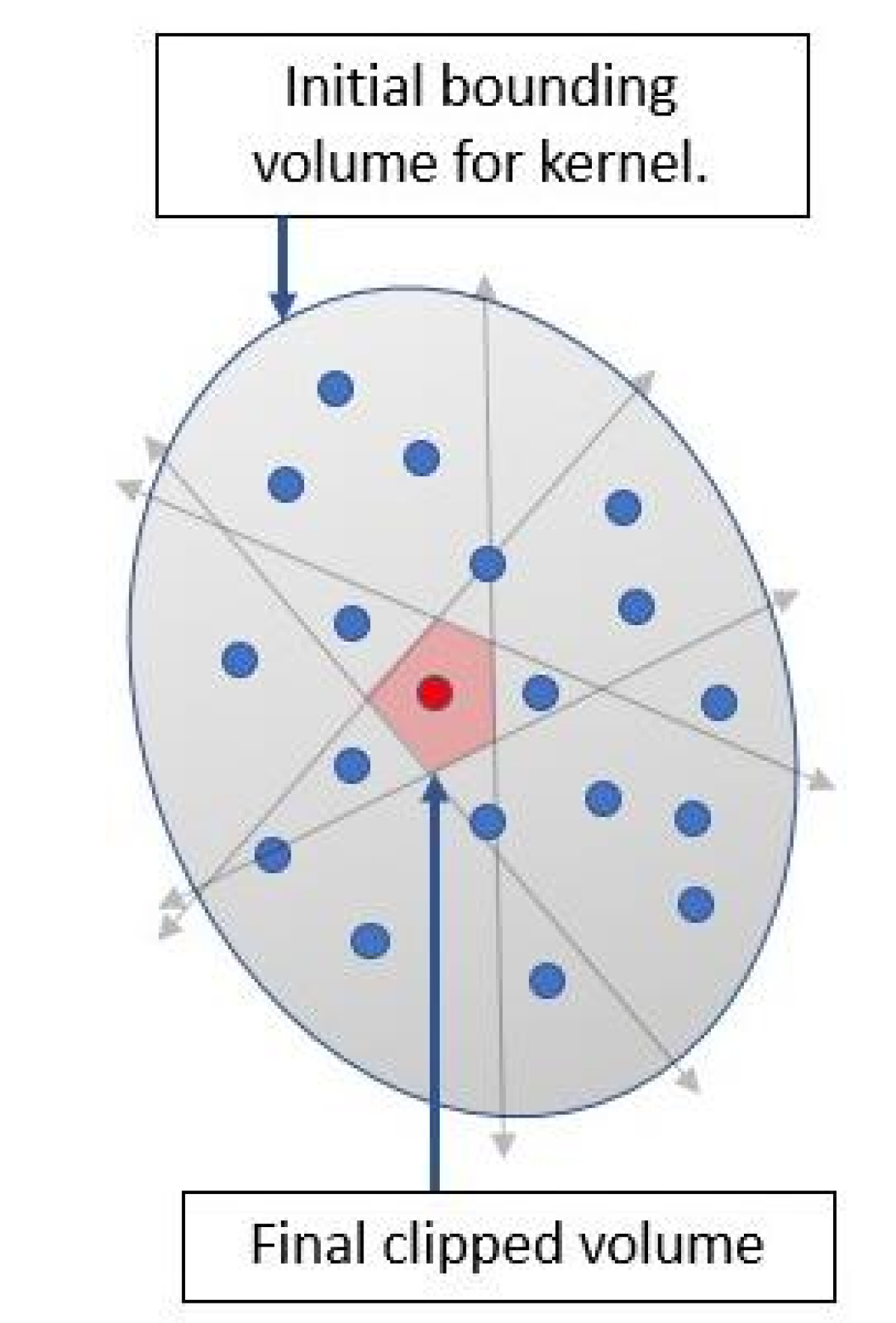
Figure 1: To construct the unique volume for the point in red, a polygon is constructed that bounds the point’s non-zero kernel volume. This polygon is then clipped by the perpendicular half-planes for each point it interacts with. For overlapping points this results in a polygon equivalent to the Voronoi tessellation for the point in question.

References

- [1] Ted Belytschko, Yury Krongauz, Daniel Organ, Mark Fleming, and Petr Krysl. Meshless methods: an overview and recent developments. Computer methods in applied mechanics and engineering, 139(1):3–47, 1996.
- [2] John I Castor. Radiation hydrodynamics. Cambridge University Press, 2004.
- [3] Stuart C Whitehouse and Matthew R Bate. Smoothed particle hydrodynamics with radiative transfer in the flux-limited diffusion approximation. Monthly Notices of the Royal Astronomical Society, 353(4):1078–1094, 2004.
- [4] Stuart C Whitehouse, Matthew R Bate, and Joe J Monaghan. A faster algorithm for smoothed particle hydrodynamics with radiative transfer in the flux-limited diffusion approximation. Monthly Notices of the Royal Astronomical Society, 364(4):1367–1377, 2005.
- [5] Serge Viau, Pierre Bastien, and Seung-Hoon Cha. An implicit method for radiative transfer with the diffusion approximation in smooth particle hydrodynamics. The Astrophysical Journal, 639(1):559, 2006.
- [6] Lucio Mayer, Graeme Lufkin, Thomas Quinn, and James Wadsley. Fragmentation of gravitationally unstable gaseous protoplanetary disks with radiative transfer. The Astrophysical Journal Letters, 661(1):L77, 2007.
- [7] Margarita Petkova and Volker Springel. An implementation of radiative transfer in the cosmological simulation code gadget. Monthly Notices of the Royal Astronomical Society, 396(3):1383–1403, 2009.
- [8] Joe J Monaghan. Smoothed particle hydrodynamics. Reports on progress in physics, 68(8):1703, 2005.
- [9] Wing Kam Liu, Sukky Jun, and Yi Fei Zhang. Reproducing kernel particle methods. International journal for numerical methods in fluids, 20(8-9):1081–1106, 1995.
- [10] Nicholas Frontiere, Cody D Raskin, and J Michael Owen. CRKSPH–a conservative reproducing kernel smoothed particle hydrodynamics scheme. Journal of Computational Physics, 332:160–209, 2017.
- [11] Hamou Sadat. On the use of a meshless method for solving radiative transfer with the discrete ordinates formulations. Journal of Quantitative Spectroscopy and Radiative Transfer, 101(2):263–268, 2006.
- [12] Hamou Sadat, Cheng-An Wang, and Vital Le Dez. Meshless method for solving coupled radiative and conductive heat transfer in complex multi-dimensional geometries. Applied Mathematics and Computation, 218(20):10211–10225, 2012.
- [13] Manuel Kindelan, Francisco Bernal, Pedro González-Rodríguez, and Miguel Moscoso. Application of the rbf meshless method to the solution of the radiative transport equation. Journal of Computational Physics, 229(5):1897–1908, 2010.
- [14] LH Liu and JY Tan. Least-squares collocation meshless approach for radiative heat transfer in absorbing and scattering media. Journal of Quantitative Spectroscopy and Radiative Transfer, 103(3):545–557, 2007.
- [15] JM Zhao, JY Tan, and LH Liu. A second order radiative transfer equation and its solution by meshless method with application to strongly inhomogeneous media. Journal of Computational Physics, 232(1):431–455, 2013.
- [16] S Kashi, A Minuchehr, A Zolfaghari, and B Rokrok. Mesh-free method for numerical solution of the multi-group discrete ordinate neutron transport equation. Annals of Nuclear Energy, 106:51–63, 2017.
- [17] LH Liu and JY Tan. Meshless local Petrov-Galerkin approach for coupled radiative and conductive heat transfer. International journal of thermal sciences, 46(7):672–681, 2007.
- [18] Brody Bassett and Brian Kiedrowski. Meshless local Petrov–Galerkin solution of the neutron transport equation with streamline-upwind petrov–galerkin stabilization. Journal of Computational Physics, 377:1–59, 2019.
- [19] JE Morel and JM McGhee. A self-adjoint angular flux equation. Nuclear Science and Engineering, 132(3):312–325, 1999.
- [20] Brody R Bassett, J Michael Owen, and Thomas A Brunner. Efficient smoothed particle radiation hydrodynamics i: Thermal radiative transfer. arXiv preprint arXiv:2001.11606, 2020.
- [21] Brody R Bassett, J Michael Owen, and Thomas A Brunner. Efficient smoothed particle radiation hydrodynamics ii: Radiation hydrodynamics. arXiv preprint arXiv:2001.11608, 2020.
- [22] Shaofan Li and Wing Kam Liu. Meshfree and particle methods and their applications. Appl. Mech. Rev., 55(1):1–34, 2002.
- [23] Vinh Phu Nguyen, Timon Rabczuk, Stéphane Bordas, and Marc Duflot. Meshless methods: a review and computer implementation aspects. Mathematics and computers in simulation, 79(3):763–813, 2008.
- [24] Satya N Atluri and Tulong Zhu. A new meshless local petrov-galerkin (mlpg) approach in computational mechanics. Computational mechanics, 22(2):117–127, 1998.
- [25] Donat Racz and Tinh Quoc Bui. Novel adaptive meshfree integration techniques in meshless methods. International journal for numerical methods in engineering, 90(11):1414–1434, 2012.
- [26] Amir Khosravifard and Mohammad Rahim Hematiyan. A new method for meshless integration in 2d and 3d galerkin meshfree methods. Engineering Analysis with Boundary Elements, 34(1):30–40, 2010.
- [27] Jiun-Shyan Chen, Cheng-Tang Wu, Sangpil Yoon, and Yang You. A stabilized conforming nodal integration for galerkin mesh-free methods. International journal for numerical methods in engineering, 50(2):435–466, 2001.
- [28] JX Zhou, JB Wen, HY Zhang, and L Zhang. A nodal integration and post-processing technique based on voronoi diagram for galerkin meshless methods. Computer methods in applied mechanics and engineering, 192(35-36):3831–3843, 2003.
- [29] MA Puso, JS Chen, E Zywicz, and W Elmer. Meshfree and finite element nodal integration methods. International Journal for Numerical Methods in Engineering, 74(3):416–446, 2008.
- [30] J Michael Owen, Jens V Villumsen, Paul R Shapiro, and Hugo Martel. Adaptive smoothed particle hydrodynamics: Methodology. ii. The Astrophysical Journal Supplement Series, 116(2):155, 1998.
- [31] J Michael Owen. Polyclipper. https://github.com/LLNL/PolyClipper, 2020.
- [32] Freddie D Witherden and Peter E Vincent. On the identification of symmetric quadrature rules for finite element methods. Computers & Mathematics with Applications, 69(10):1232–1241, 2015.
- [33] Satya N Atluri, H-G Kim, and J Ya Cho. A critical assessment of the truly meshless local petrov-galerkin (mlpg), and local boundary integral equation (lbie) methods. Computational mechanics, 24(5):348–372, 1999.
- [34] Michael A Heroux, Roscoe A Bartlett, Vicki E Howle, Robert J Hoekstra, Jonathan J Hu, Tamara G Kolda, Richard B Lehoucq, Kevin R Long, Roger P Pawlowski, Eric T Phipps, et al. An overview of the trilinos project. ACM Transactions on Mathematical Software (TOMS), 31(3):397–423, 2005.
- [35] Joshua J Jarrell and Marvin L Adams. Discrete-ordinates quadrature sets based on linear discontinuous finite elements. In International Conference on Mathematics and Computational Methods Applied to Nuclear Science and Engineering (M&C 2011), Rio de Janeiro, RJ, Brazil, 2011.
- [36] RP Smedley-Stevenson, AW Hagues, and J Kphzi. A benchmark for assessing the effectiveness of diffusion synthetic acceleration schemes. In Proceedings of the Joint International Conference on Mathematics and Computation, Supercomputing in Nuclear Applications and the Monte Carlo Method (M&C 2015), Nashville, TN, 2015.
- [37] Ben C Yee, Samuel S Olivier, Terry S Haut, Milan Holec, Vladimir Z Tomov, and Peter G Maginot. A quadratic programming flux correction method for high-order dg discretizations of sn transport. Journal of Computational Physics, page 109696, 2020.
- [38] Keisuke Kobayashi, Naoki Sugimura, and Yasunobu Nagaya. 3D radiation transport benchmark problems and results for simple geometries with void region. Progress in Nuclear Energy, 39(2):119–144, 2001.
- [39] Steven Hamilton, Michele Benzi, and Jim Warsa. Negative flux fixups in discontinuous finite element sn transport. In International Conference on Mathematics, Computational Methods and Reactor Physics (M&C 2009), American Nuclear Society, LaGrange Park, Illinois, USA. Citeseer, 2009.
- [40] James S Warsa, Todd A Wareing, and Jim E Morel. Krylov iterative methods and the degraded effectiveness of diffusion synthetic acceleration for multidimensional sn calculations in problems with material discontinuities. Nuclear science and engineering, 147(3):218–248, 2004.
- [41] TERRY S Haut, BS Southworth, PETER G Maginot, and VLADIMIR Z Tomov. Dsa preconditioning for dg discretizations of {} transport and high-order curved meshes. arXiv preprint arXiv:1810.11082, 2018.