Machine Learning in Nano-Scale
Biomedical Engineering

Abstract

Machine learning (ML) empowers biomedical systems with the capability to optimize their performance through modeling of the available data extremely well, without using strong assumptions about the modeled system. Especially in nano-scale biosystems, where the generated data sets are too vast and complex to mentally parse without computational assist, ML is instrumental in analyzing and extracting new insights, accelerating material and structure discoveries and designing experience as well as supporting nano-scale communications and networks. However, despite these efforts, the use of ML in nano-scale biomedical engineering remains still under-explored in certain areas and research challenges are still open in fields such as structure and material design and simulations, communications and signal processing, and bio-medicine applications. In this article, we review the existing research regarding the use of ML in nano-scale biomedical engineering. In more detail, we first identify and discuss the main challenges that can be formulated as ML problems. These challenges are classified in three main categories: structure and material design and simulation, communications and signal processing and biomedicine applications. Next, we discuss the state of the art ML methodologies that are used to countermeasure the aforementioned challenges. For each of the presented methodologies, special emphasis is given to its principles, applications and limitations. Finally, we conclude the article with insightful discussions, that reveal research gaps and highlight possible future research directions.

Nomenclature

2D

Two dimensional

3D

Three dimensional

ANI

Accurate neural network engine for molecular energies

AL

Active Learning

AdaBoost

Adaptive Boosting

AEV

Atomic Environments Vector

ANN

Artificial Neural Network

ANOVA

Analysis of Variance

ARES

Autonomous Research System

Bagging

Bootstrap Aggregating

BER

Bit Error Rate

BPN

Behler-Parrinello Network

BSS

Blind Source Separation

CG

Coarse Graining

CGN

Coarse Graining Network

CMOS

Complementary Metal-Oxide-Semiconductor

CNN

Convolution Neural Network

DCF

Discrete Convolution Filter

DNN

Deep Neural Network

D²NN

Diffractive Deep Neural Network

DPN

Deep Potential Network

DT

Decision Table

DTL

Decision Tree Learning

DTNB

Decision Table Naive Bayes

DTNN

Deep Tensor Neural Network

EEG

Electroencephalography

FS

Feature Selection

FSC

Feedback System Control

GAN

Generative Adversarial Network

GD

Gradient Descent

GRNN

Generalized Regression Neural Network

ICA

Independent Component Analysis

ISI

Inter-Symbol Interference

KNN

k-Nearest Neighbor

LDA

Linear Discriminant Analysis

LR

Logistic Regression

LWL

Local Weighted Learning

MAN

Molecular Absorption Noise

MC

Molecular Communications

MIMO

Multiple-Input Multiple-Output

ML

Machine Learning

MLP

Multi-layer Perceptron

ML-SF

Machine Learning Scoring Function

MvLR

Multivariate linear regression

NBTree

Naive Bayes Tree

NN

Neural Network

NNP

Neural Network Potential

NP

Nano-Particles

PAMAM

Polyamidoamine

PCA

Principal Component Analysis

PDF

Probability Density Function

PES

Potential Energy Surface

PSO

Particle Swarm Optimization

QM

Quantum Mechanic

QP

Quadratic Programming

QPOP

Quadratic Phenotype Optimization Platform

QSAR

Quantitative Structure-activity relationships

RELU

REctified Linear Unit

RForest

Random Forest

RNAi

Ribonucleic acid interference

RNN

Recurrent Neural Network

SDR

Standard Deviation Reduction

SF

Scoring Functions

SiC

Silicon Carbide

SmF

Symmetry Function

SMO

Sequential Minimal Optimization

SOTA

State Of The Art

SVM

Support Vector Machine

TEM

Transmission Electron Microscope

THz

Terahertz

ZnO

Zinc Oxide

I Introduction

In 1959, Richard P. Feynman articulated “It would be interesting if you could shallow the surgeon. You put the mechanical surgeon inside the blood vessel and it goes into the heart and looks around… other small machines might be permanently incorporated in the body to assist some inadequately-functioning organ.” More than half a century later, this quote is still state-of-the-art (SOTA). Currently, nanotechnology revisits the conventional therapeutic approaches by producing more than $100$ nano-material based drugs. These have already been approved or they are under clinical trial [1], while discussing the utilization of nano-scale communication networks for real time monitoring and precision drug delivery [2, 3]. However, these developments come with the need of analyzing vast and complicated, as well as rich in relations, data sets.

Fortunately, in the last couple of decades, we have witnessed a revolutionary development of new tools from the field of machine learning (ML), which enables the analysis of large data sets through training models. These models can be utilized for observations classification or predictions and have been considered in several engineering fields, including computer vision, speech and image recognition, natural language processing, etc. This frontier is continuing its expansion into several other scientific domains, such as quantum physics, chemistry and biology, and is expected to make a significant impact on the design of novel nano-materials and structures, nano-scale communication systems and networks, while simultaneously presenting new data-driven biomedicine applications [4].

In the field of nano-materials and structure design, experimental and computational simulating methodologies have traditionally been the two fundamental pillars in exploring and discovering properties of novel constructions as well as optimizing their performance [5]. However, these methodologies are constrained by experimental conditions and limitation of the existing theoretical knowledge. Meanwhile, as the chemical complexity of nano-scale heterogeneous structures increases, the two traditional methodologies are rendered incapable of predicting their properties. In this context, the development of data-driven techniques, like ML, becomes very attractive. Similarly, in nano-scale communications and signal processing, the computational resources are limited and the major challenge is the development of low-complexity and accurate system models and data detection techniques, that do not require channel knowledge and equalization, while taking into account the environmental conditions (e.g., specific enzyme composition). To address these challenges the development of novel ML methods is deemed necessary [6]. Last but not least, ML can aid in devising novel, more accurate methods for disease detection and therapy development, by enabling genome classification [7] and selection of the optimum combination of drugs [8].

Motivated from above, the present contribution provides an interdisciplinary review of the existing research from the areas of nano-engineering, biomedical engineering and ML. To the best of the authors knowledge no such review exists in the technical literature, that focuses on the ML-related methodologies that are employed in nano-scale biomedical engineering. In more detail, the contribution of this paper is as follows:

• The main challenges-problems in nano-scale biomedical engineering, which can be tackled with ML techniques, are identified and classified in three main categories, namely: structure and material design and simulations, communications and signal processing, and bio-medicine applications.

• SOTA ML methodologies, which are used in the field of nano-scale biomedical engineering, are reviewed, and their architectures are described. For each one of the presented ML methods, we report its principles and building blocks. Finally, their compelling applications in nano-scale biomedicine systems are surveyed for aiding the readers in refining the motivation of ML in these systems, all the way from analyzing and designing new nano-materials and structures to holistic therapy development.

• Finally, the advantages and limitations of each ML approach are highlighted, and future research directions are provided.

The rest of the paper is organized as follows: Section II identifies the nano-scale biomedical engineering problems that can be solved with ML techniques. Section III presents the most common ML approaches related to the field of nano-scale biomedical engineering. Section IV explains the advantages and limitations of the ML approaches alongside their applications and extracts future directions. Section V concludes this paper and summarizes its contribution. The structure of this treatise is summarized at a glance in Fig. 1.

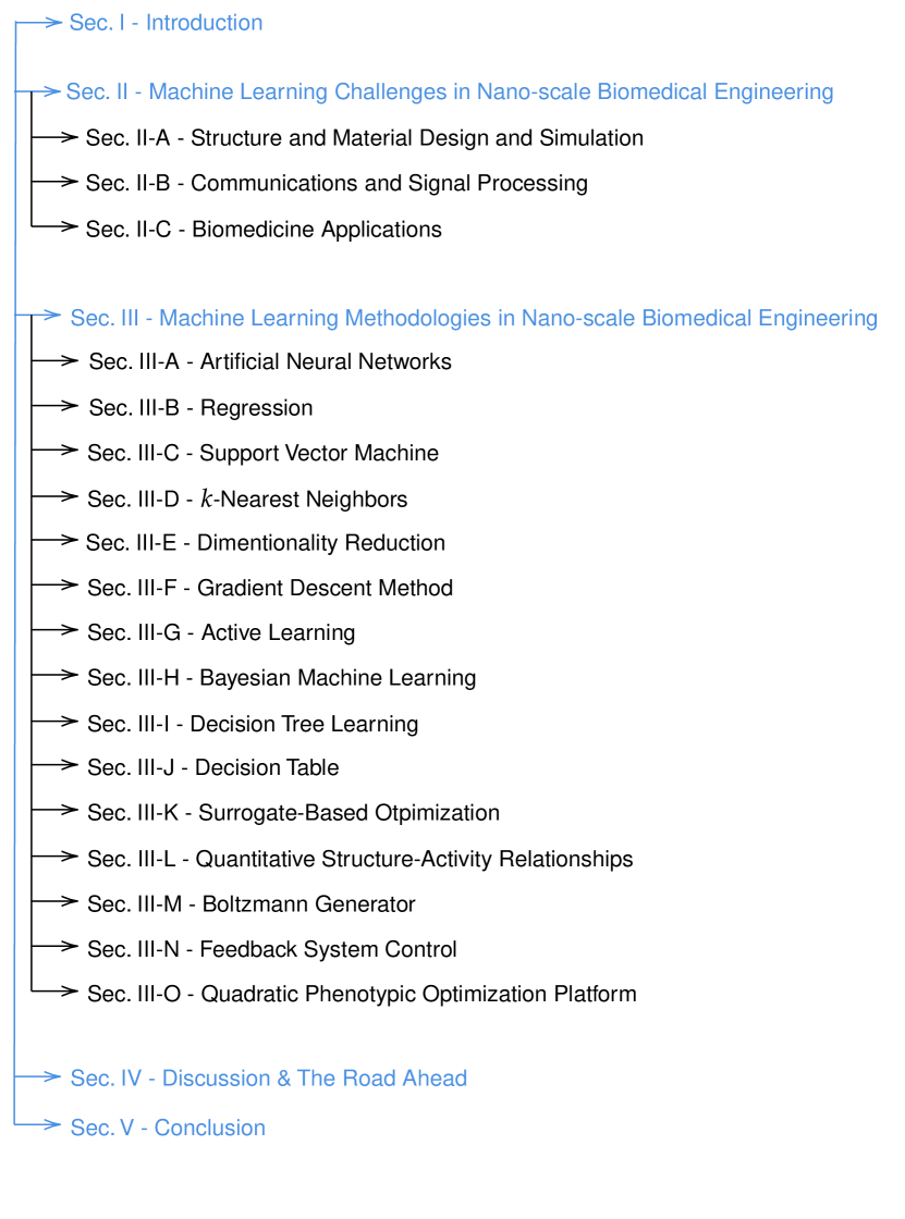
Figure 1: The structure of this treatise.

II Machine Learning Challenges in Nano-scale Biomedical Engineering

In this section, we report how several of the open challenges in nano-scale biomedical engineering has already been and can be formulated to ML problems. As mentioned in the previous section, in order to provide a better understanding of the nature of these challenges, we classify them into three categories, i.e. i) structure and material design and simulation, ii) communications and signal processing, and iii) biomedicine applications. Following this classification, which is illustrated in Fig. 2, the rest of this section is organized as follows: Section II-A focuses on presenting the challenges on designing and simulating nano-scale structures, materials and systems, whereas, Section II-B discusses the necessity of employing ML in nano-scale communications. Similarly, Section II-C emphasizes in the possible applications of ML in several applications, such as therapy development, drug delivery and data analysis.

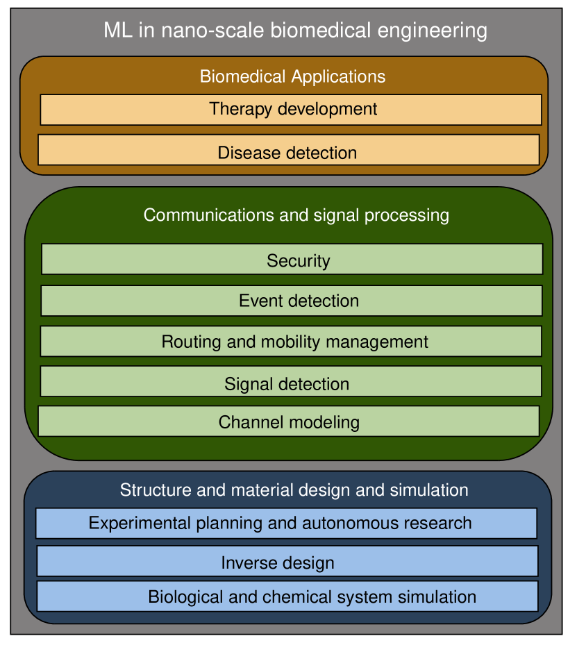
Figure 2: ML challenges in nano-scale biomedical engineering.

II-A Structure and Material Design and Simulation

One of the fundamental challenges in material science and chemistry is the understanding of the structure properties  [9]. The complexity of this problem grows dramatically in the case of nanomaterials because: i) they adopt different properties from their bulk components; and ii) they are usually hetero-structures, consisting of multiple materials. As a result, the design and optimization of novel structures and materials, by discovering their properties and behavior through simulations and experiments, lead to multi-parameter and multi-objective problems, which in most cases are extremely difficult or impossible to be solved through conventional approaches; ML can be an efficient alternative choice to this challenge.

II-A1 Biological and chemical systems simulation

In atomic and molecular systems, there exist complex relationships between the atomistic configuration and the chemical properties, which, in general, cannot be described by explicit forms. In these cases, ML aims to the development of associate configurations by means of acquiring knowledge from experimental data. Specifically, in order to incorporate quantum effects on molecular dynamics simulations, ML can be employed for the derivation of potential energy surfaces (PESs) from quantum mechanic (QM) evaluations [10, 11, 12, 13, 14, 15]. Another use of ML lies in the simulation of molecular dynamic trajectories. For example, in [16, 17, 18], the authors formulated ML problems for discovering the optimum reaction coordinates in molecular dynamics, whereas, in [19, 20, 21, 22, 23], the problem of estimating free energy surfaces was reported. Furthermore, in [24, 25, 26, 27], the ML problem of creating Markov state models, which take into account the molecular kinetics, was investigated. Finally, the ML use in generating samples from equilibrium distributions, that describe molecular systems, was studied in [28].

II-A2 Inverse design

The availability of several high-resolution lithographic techniques opened the door to devising complex structures with unprecedented properties. However, the vast choices space, which is created due to the large number of spatial degrees of freedom complemented by the wide choice of materials, makes extremely difficult or even impossible for conventional inverse design methodologies to ensure the existence or uniqueness of acceptable utilizations. To address this challenge, nanoscience community turned their eyes to ML. In more detail, several researchers identified three possible methods, which are based on artificial neural networks (ANNs), deep neural networks (DNNs), and generative adversarial networks (GANs). ANNs follow a trail-and-error approach in order to design multilayer nanoparticles (NP) [29]. Meanwhile, DNNs are used in the metasurface design [30]. Finally, GANs can be used to design nanophotonics structures with precise user-define spectral responses [31].

II-A3 Experiments planning and autonomous research

ML has been widely employed, in order to efficiently explore the vast parameter space created by different combinations of nano-materials and experimental conditions and to reduce the number of experiments needed to optimize hetero-structures (see e.g., [32] and references therein). Towards this direction, fully autonomous research can be conducted, in which experiments can be designed based on insights extracted from data processing through ML, without human in the loop  [33].

II-B Communications and Signal Processing

In biomedical applications, nano-sensors can be utilized for a variety of tasks such as monitoring, detection and treatment [34, 35]. The size of such nano-sensors ranges between $1-100\text{ }\mathrm{nm}$, which refers to both macro-molecules and bio-cells [35]. The proper selection of size and materials is critical for the system performance, while it is constrainted by the target area, their purpose, and safety concerns. Such nano-networks are inspired by living organisms and, when they are injected into the human body, they interact with biological processes in order to collect the necessary information [36]. However, they are characterized by limited communication range and processing power, that allow only short-range transmission techniques to be used [37]. As a consequence, conventional electromagnetic-based transmission schemes may not be appropriate for communications among molecules [38, 3], since, in molecular communications the information is usually encoded in the number of released particles. The simplest approach for the receiver to demodulate the symbol is to compare the number of received particles with predetermined thresholds. In the absence of inter-symbol interference (ISI), finding the optimal thresholds is a straightforward process. However, in the presence of ISI the threshold needs to be extracted as a solution of the error probability minimization (or performance maximization) problem [39, 40, 41]. The aforementioned approaches require knowledge of the channel model. However, in several practical scenarios, where the molecular communications (MC) system complexity is high, this may not be possible. To countermeasure this issue, ML methods can be employed to accurately model the channel or perform data sequence detection.

An alternative to MCs that has been used to support nano-networks is communications in the terahertz (THz) band. For these networks, apart from their specifications, an accurate model for the THz communication between nano-sensors is imperative for their simulation and performance assessment. In addition, another problem that is entangled with novel nano-sensor networks is their resilience against attacks, which is of high importance since not only the system reliability is threatened, but also the safety of the patients is at stake. Thus, it is imperative for any possible threats to be recognized and for effective countermeasures to be developed. A solution to the above problems appears to be relatively complex for conventional computational methods. On the other hand, ML can provide the tools to model the space-time trajectories of nano-sensors in the complex environments of the human body as well as to draw strategies that mitigate the security risks of the novel network architectures.

II-B1 Channel modeling

One of the fundamental problems in MCs is to accurately model the channel in different environments and conditions. Most of the MC models assume that a molecule is removed from the environment after hitting the receiver [42, 43, 44, 45, 46]; hence, each molecule can contribute to the received signal once. To model this phenomenon, a first-passage process is employed. Another approach was created from the assumption that molecules can pass through the receiver [47, 48, 49, 50]. In this case, a molecule contributes multiple times to the received signal. However, neither of the aforementioned approaches are capable of modeling perfectly absorbing receivers, when the transmitters reflect spherical bodies. Interistingly, such models accommodate practical scenarios where the emitter cells do not have receptors at the emission site and they cannot absorb the emitted molecules. An indicative example lies in hormonal secretion in the synapses and pancreatic $\beta-$cell islets [51]. To fill this gap, ML was employed in [52, 53] to model molecular channels in realistic scenarios, with the aid of ANNs. Similarly, in THz nano-scale networks, where the in-body environment is characterized by high path-loss and molecular absorption noise (MAN), ML methods can be used in order to accurately model MAN. This opens the road to a better understanding of the MAN’s nature and the design of new transmission schemes and waveforms.

II-B2 Signal detection

To avoid channel estimation in MC, Farsal et al. proposed in  [54] a sequence detection scheme, based on recurrent neural networks (RNNs). Compared with previously presented ISI mitigation schemes, ML-based data sequence detection is less complex, since they do not require to perform channel estimation and data equalization. Following a similar approach, in [6], the authors presented an ANN capable of achieving the same performance as conventional detection techniques, that require perfect knowledge of the channel.

In THz nano-scale networks, an energy detector is usually used to estimate the received data [55]. In more detail, if the received signal power is below a predefined threshold, the detector decides that the bit $0$ has been sent, otherwise, it decides that $1$ is sent. However, the transmission of $1$ causes a MAN power increase, usually capable of affecting the detection of the next symbols. To counterbalance this, without increasing the symbol duration, a possible approach is to design ML algorithms that are trained to detect the next symbol and take into account the already estimated ones. Another ML challenge in signal detection at THz nano-scale networks, lies with detecting the modulation mode of the transmission signal by a receiver, when no prior synchronization between transmitter and receiver has occurred. The solution to this problem will provide scalability to these networks. Motivated by this, in [56], the authors provided a ML algorithm for modulation recognition and classification.

II-B3 Routing and mobility management

In THz nano-scale networks, the design of routing protocols capable of proactively countermeasuring congestion has been identified as the next step for their utilization [57]. These protocols need to take into account the extremely constrained computational resources, the stochastic nature of nano-nodes movements as well as the existence of obstacles that may interrupt the line-of-sight transmission. The aforementioned challenges can be faced by employing SOTA ML techniques for analyzing collected data and modeling the nano-sensors’ movements, discovering neighbors that can be used as intermediate nodes, identifying possible blockers, and proactively determining the message root from the source to the final destination. In this context, in [58], the authors presented a multi-hop deflection routing algorithm based on reinforcement learning and analyzed its performance in comparison to different neural networks (NNs) and decision tree updating policies.

II-B4 Event detection

Nano-sensor biomedicine networks can provide continuous monitoring solutions, that can be used as compact, accurate, and portable diagnostic systems. Each nano-sensor obtains a biological signal linked to a specific disease and is used for detecting physiological change or various biological materials [59]. Successful applications in event detection include monitoring of DNA interactions, antibody, and enzymatic interactions, or cellular communication processes, and are able to detect viruses, asthma attacks and lung cancer [60]. For example, in [61], the authors developed a bio-transferrable graphene wireless nano-sensor that is able to sense extremely sensitive chemicals and biological compounds up to single bacterium. Furthermore, in [62], a Sandwich Assay was developed that combines mechanical and optoplasmonic transduction in order to detect cancer biomarkers at extremely low concentrations. Also, in [63], a molecular communication-based event detection network was proposed, that is able to cope with scenarios where the molecules propagate according to anomalous diffusion instead of the conventional Brownian motion.

II-B5 Security

Although, the emergence of nano-scale networks based on both electromagnetic and MCs opened opportunities for the development of novel healthcare applications, it also generated new problems concerning the patients’ safety. In particular, two types of security risks have been observed, namely blackhole and sentry attacks [64]. In the former, malicious nano-sensors emit chemicals to attract the legitimate ones and prevent them from searching for their target. On the contrary, in the latter, the malicious nano-sensors repel the legitimate ones for the same reason. Such security risks can be counterbalanced with the use of threshold-based and bayesian ML techniques that have been proven to counter the threats with minimal requirements.

II-C Biomedicine Applications

Timely detection and intervention are tied with successful treatment for many diseases. This is the so-called proactive treatment and is one of the main objectives of the next-generation healthcare systems, in order to detect and predict diseases and offer treatment services seamlessly. Data analysis and nanotechnology progress simultaneously toward the realization of these systems. Recent breakthroughs in nanotechnology-enabled healthcare systems allow for the exploitation of not only the data that already exist in medical databases throughout the world, but also of the data gathered from millions of nano-sensors.

II-C1 Disease detection

One of the most common problems in healthcare systems is genome classification, with cancer detection being the most popular. Various classification algorithms are suitable for tackling this problem, such as Naive Bayes, k-Nearest Neighbors, Decision tree, ANNs and support vector machine (SVM) [65]. For example, the authors in [66], predicted the risk of cerebral infarction in patients by using demographic and cerebral infarction data. In addition, in [7] a unique coarse-to-fine learning method was applied on genome data to identify gastric cancer. Another example is the research presented in [67], where SVM and convolution NNs (CNNs) were used to classify breast cancer subcategory by performing analysis on microscopic images of biopsy.

II-C2 Therapy development

Therapy development and optimization can improve clinical efficacy of treatment for various diseases, without generating unwanted outcomes. Optimization still remains a challenging task, due to its requirement for selecting the right combination of drugs, dose and dosing frequency [68]. For instance, a quadratic phenotype optimization platform (QPOP) was proposed in [69] to determine the optimal combination from 114 drugs to treat bortezomib-resistant multiple myeloma. Since its creation, QPOP has been used to surpass the problems related to drug designing and optimization, as well as drug combinations and dosing strategies. Also, in [70], the authors presented a platform called CURATE.AI, which was validated clinically and was used to standardize therapy of tuberculosis patients with liver transplant-related immunosuppression. Furthermore, CURATE.AI was used for treatment development and patient guidance that resulted in halted progression of metastatic castration resistant prostate cancer  [71].

III Machine Learning Methods in Nano-scale Biomedical Engineering

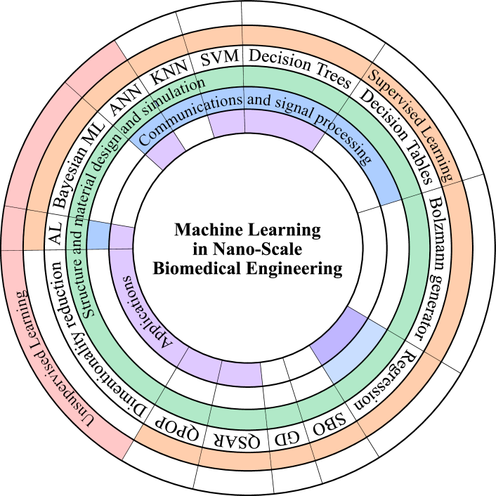
Figure 3: ML methodologies for nano-scale biomedical engineering.

This section presents the fundamental ML methodologies that are used in nano-scale biomedical engineering. As illustrated in Fig. 3, in nano-scale biomedical engineering, depending on how training data are used, we can identify two groups of ML methodologies, namely supervised, and unsupervised learning.

Supervised learning methodologies require a certain amount of labeled data for training [72]. Their objective is to create a function that maps the input data to the output labels relying on the initial training. In more detail, supervised learning return a mapping function $g(x)$ that maximizes the scoring function $f(x_{n},y_{n})$ for each $n\in[1,N]$, with $x_{n}$ being the $n-$th sample of the input training data, $y_{n}$ representing the label of $x_{n}$, and $N$ being the size of the training set. Of note, in most realistic scenarios, the aforementioned sets are independent and identical distributed.

On the other hand, unsupervised learning methodologies aim at exploring the hidden features or structure of data without relying on training sets [73]. Therefore, they have extensively been used for chemical and biological properties discovery in nano-scale structures and materials. The disadvantage of unsupervised learning methodologies lies to the fact that no standard accuracy evaluation method for their output, due to the lack of training data sets.

The rest of this section is organized as follows: Section III-A provides a survey of the ANNs, which are employed in this field, while Section III-B presents regression methodologies. Meanwhile, the applications, architecture and building blocks of SVMs and $k-$nearest neighbors (KNNs) are respectively described in Sections III-C and III-D, whereas dimentionality reduction methods are given in Section III-E. A brief review of gradient descent (GD) and active learning (AL) methods are respectively delivered in Sections III-F and III-G. Furthermore, Bayesian ML is discussed in Section III-H, whereas decision tree learning (DTL) and decision table (DT) based algorithms are respectively reported in Sections III-I and III-J. Section III-K revisits the operating principles of surrogate-based optimization, while Section III-L describes the use of quantitative structure-activity relationships (QSARs) in ML. Finally, the Boltzmann generator is presented in Section III-M, while Sections III-N and III-O respectively discuss feedback system control (FSC) methods and the quadratic phenotypic optimization platform. The organization of this section is summarized at a glance in Fig. 4.

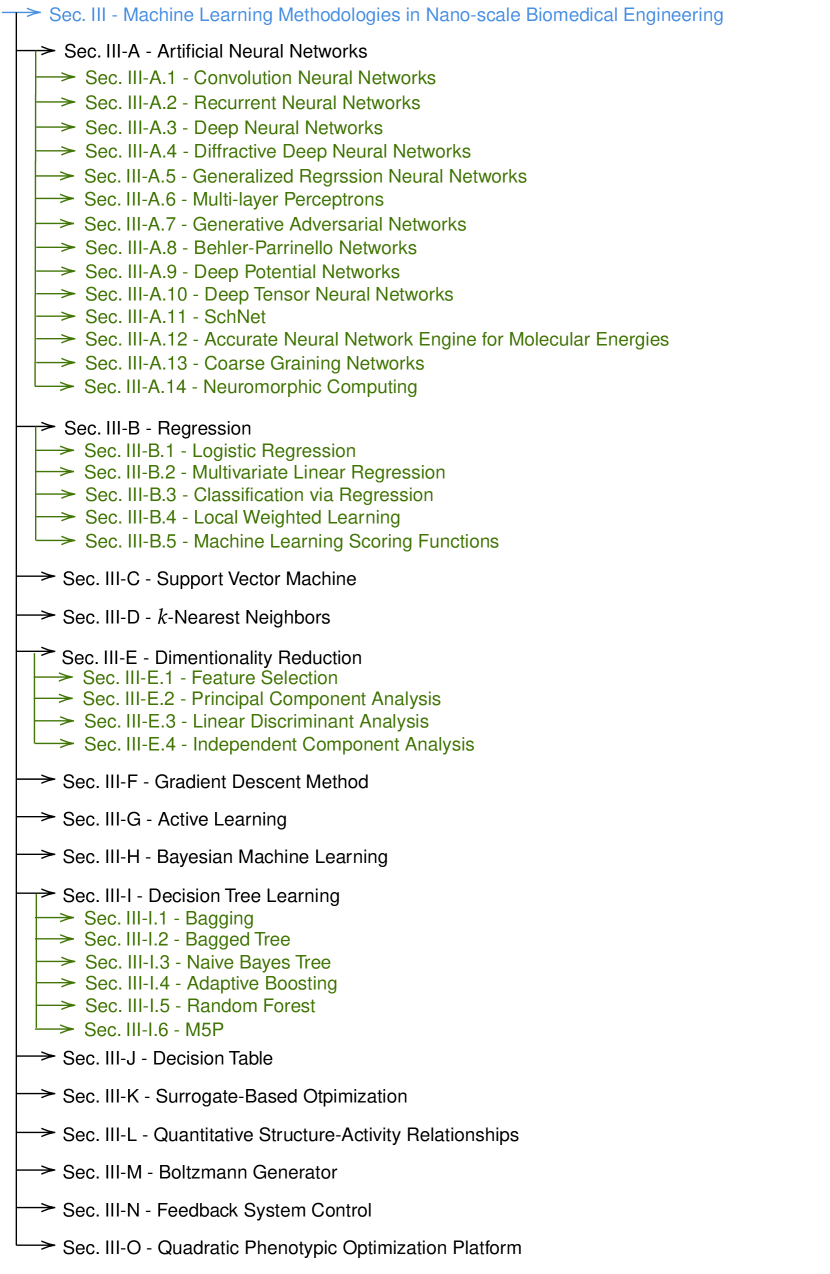
Figure 4: The organization of Section III.

III-A Artificial Neural Networks

ANNs can be used for both classification and regression. Their operation principle is based on the linear and/or non-linear manipulation of the input-data in several intermediate (hidden) layers. The output of each layer is subjected to by some non-linear functions, namely activation functions. This can be formulated as

$$y_{k}=g\left(v_{k}+c_{k}\right),$$ (1)

where

$$v_{k}=\sum_{i=1}^{m}w_{ki}x_{i},$$ (2)

with $x_{i}$ and $y_{k}$ respectively being the input and the output signals of the $k$-th layer, while $w_{ki}$ and $c_{k}$ respectively standing for the associated weights and bias. Finally, $g(\cdot)$ stands for the activation function. This process allows us to model complex relationships of the processed data.

The reminder of this Section is focused on presenting the ANNs that are commonly used in nano-scale biomedical engineering and is organized as follows: Section III-A1 reports the applications of CNNs in this field, presents a typical CNN architecture and discusses its building blocks functionalities. Similarly, Section III-A2 presents the operation of RNNs, while deep NNs (DNNs) are discussed in Section III-A3. Diffractive DNNs (D²NN) and generalized regression NNs (GRNNs) are respectively described in Section III-A4 and III-A5, while Sections III-A6 and III-A7 respectively revisit the multi-layer perceptrons (MLPs) and GANs. Moreover, the applications, architecture and limitations of Behler-Parrinello networks (BPNs) are reported in Section III-A8, whereas, Sections III-A9, III-A10, and III-A11 respectively present the ones of deep potential networks (DPNs), deep tensor NNs (DTNNs), and SchNets. Likewise, the usability and building blocks of accurate NN engine for molecular energies, or as is widely-known ANI, are provided in Section III-A12. Finally, comprehensive descriptions of coarse graining networks (CGNs) and neurophormic computing are respectively given in Sections III-A13 and III-A14. Table I summarizes some of the typical applications of ANNs in nano-scale biomedical engineering.

TABLE I: ANN applications in nano-scale biomedical engineering.

Paper	Application	Method	Description
[18]	Chemical properties discovery	CGN	Prediction of the rototranslationally invariant energy in QM
[31]	Nano-material inverse design	GAN	Metasurfaces inverse design
[53]	Channel modelling	DNN	MIMO channel modeling in MC
[54]	Sequence detection	RNN	Data sequence detection in MC
[74]	Image analysis	CNN	Skyrmions analysis in labeled Lorentz TEM images
[75]	Image analysis	CNN	Matter phases identification
[76]	ARES	CNN	State-of-the-tip identification in tunneling microscopy scanning
[77]	Image analysis	RNN	Nano-structure design
[78]	Sequence detection	RNN	Data sequence detection in MC
[79]	Feature detection and object classification	D2NN	Classification of images and creation of imaging lens at THz spectrum
[80]	Data analysis	GRNN, MLP, BPN	Characterization of psychological wellness from survey results
[81]	Nano-structure properties discovery	GRNN	Study of the impact of ZnO NPs suspensions in diesel and Mahua
			biodiesel blended fuel
[82]	Nano-structure properties discovery	GRNN	Prediction of the pool boiling heat transfer coefficient of refrigerant-based
			nano-fluids
[83]	Nano-structure analysis	MLP	Analysis of the crystalline structure of magnesium oxide films grown over
			6H SiC substrates
[84]	Nano-structure design	GAN	Nano-photonic structure design
[85]	Chemical properties discovery	BPN	Energy surfaces prediction from QM data
[86]	Complex structure simulation	BPN	Self-learning Monte Carlo creation for many-body interactions
[87]	Complex structure simulation	BPN	Atomic energy prediction
[88]	Chemical properties discovery	DPN	PES prediction that use atomic configuration directly at the input data
[89]	Molecules and nano-material properties	DTNN	General QM molecular potential modeling
	discovery
[90]	Chemical properties discovery	SchNet	PES prediction that takes into account rototranslationally invariant
			inter-atomic distances
[91]	Chemical properties modeling	ANI	Prediction of molecules energies in complex nano-structures
[92]	Chemical properties modeling	CGN	Theormodynamics prediction in chemical systems
[93]	Chemical properties modeling	CGN	Theormodynamics prediction in chemical systems

III-A1 Convolution Neural Networks

CNNs have been extensively used for analyzing images with some degrees of spatial correlation [94, 95, 96, 97]. The aim of CNNs is to extract fundamental local correlations within the data, and thus, they are suitable for identifying image features that depend on these correlations. In this sense, in [74], the author employed CNNs to analyze skyrmions in labeled Lorentz transmission electron microscope (TEM) images, while, in [75], CNNs were used to identify matter phases from data extracted via Monte Carlo simulations. Another application of CNNs in nano-scale biomedical systems lies in the utilization of autonomous research systems (ARES) [76]. Specifically, in [76], the authors presented a learning method that determines the state-of-the-tip in scanning tunneling microscopy.

Figure 5 depicts a typical CNN architecture, which mimics the neurons’ connectivity patterns in the human brain. It consists of neurons, which are arranged in a three dimensional (3D) space, i.e., width, height, and depth. Each neuron receives several inputs and performs an element-wise multiplication, which is usually followed by a non-linear operation. Note that, in most cases, CNN architectures are not fully-connected. This means that the neurons in a layer will only be connected to a small region of the previous layer. Each layer of a CNN transforms its input to a 3D output of neuron activations. In more detail, it consists of the following layers:

• Input: This layer represents the input image into the CNN. Input layer holds the raw pixels of the image in the three color channels, namely red, green, and blue.

• Convolution: layers are the pillars of CNN. They contain the weights that are used to extract the distinguished features of the images. As illustrated in Fig. 5, they evaluate the output of neurons, which are connected to local regions in the input.

• Rectified linear unit (RELU): applies an element-wise activation function, such as thresholding at zero. This allows the generation of non-linear decision boundaries.

• Pooling: conducts downsampling along the spatial dimensions.

• Flattening: reorganizes the values of the 3D matrix into a vector.

• Hidden layers: returns the classification scores.

Figure 5: CNN architecture.

III-A2 Recurrent Neural Networks

Most ML networks rely to the assumption of independence among the training and test data. Thus, after processing each data point, the entire state of the network is lost. Apparently, this is not a problem, if the data points are independently generated. However, if they are in time or space related, the aforementioned assumption becomes unacceptable. Moreover, conventional networks usually rely on data points, which can be organized in vectors of fixed length. However, in practice, there exist several problems, which require modeling data with temporal or sequential structure and varying length inputs and outputs.

In order to overcome the aforementioned limitations, RNNs have been proposed in [98]. RNNs are connectionist models capable of selectively passing information across sequence steps, while processing sequential data. From the nano-scale applications point of view, RNNs have been used for nano-structure design and data sequence detection in MCs. Specifically, in [77], Hedge described the role that RNNs are expected to play in the design of nano-structures, while, in [78] and in [54], the authors employed a RNN in order to train a maximum likelihood detector in MCs systems.

Figure 6 depicts the most successful RNN architecture, introduced by Hochreiter and Schmidhuber [99]. From this figure, it is evident that the only difference between RNN and CNN is the fact that the hidden layers of the latter are replaced with memory cells with self-connected recurrent fix-weighted edges. The memory cells store the internal state of the RNN and allow processing sequences of inputs of varying length. Likewise, the recurrent edges guarantee that the gradient can pass across several steps without vanishing. The weights change during training in a slowing rate in order to create a long-term memory. Finally, RNNs support short-term memory through ephemeral activations, which pass from each node to successive nodes. This allows RNNs to exploit the dynamic temporal information hidden in time sequences.

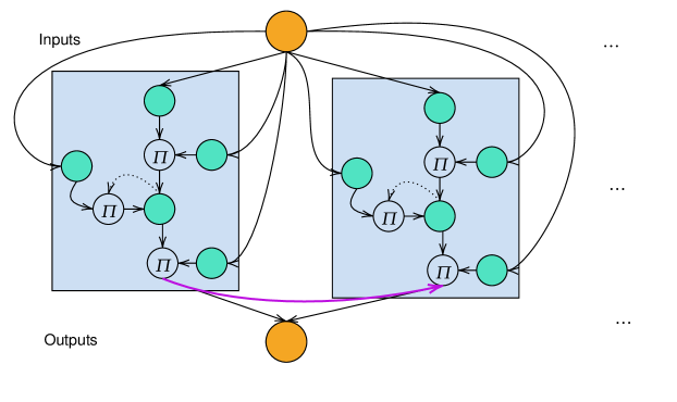
Figure 6: An RNN with a hidden layer consisting of two memory cells.

III-A3 Deep Neural Networks

Deep learning was suggested in [54] as an efficient method to detect the information at the receiver in MCs. Specifically, based on the similarities between speech recognition and molecular channels, techniques from DL can be utilized to train a detection algorithm from samples of transmitted and received signals. In the same work, it was proposed that well-known NNs such as an RNN, can train a detector even if the underlying system model is not known. Furthermore, a real-time NN-based sequence detector was proposed, and it was shown that the suggested DL-based algorithms could eliminate the need for instantaneous channel state information estimation.

In another research work, [53], a NN-based modeling of the molecular multiple-input multiple-output (MIMO) channel, was presented. This is a remarkable contribution, since the proposed model can be used to investigate the possibility of increasing the low rates in MCs. Specifically, in this paper a $2\times 2$ molecular MIMO channel was modeled through two ML-based techniques and the developed model was used to evaluate the bit error rate (BER).

III-A4 Diffractive Deep Neural Networks

In [79], a diffractive deep NN ($\text{D}^{2}$NN) framework was proposed. The $\text{D}^{2}$NN is an all-optical deep learning framework, where multiple layers of diffractive surfaces physically form the NN. These layers collaborate to optically perform an arbitrary function, which can be learned statistically by the network. The learning part is performed through a computer, whereas the prediction of the physical network follows an all-optical approach.

Several transmissive and/or reflective layers create the $\text{D}^{2}$NN. More specifically, each point on a specific layer can either transmit or reflect the incoming wave. To this end, an artificial neuron is formed, which is connected to other neurons of the following layers through optical diffraction. Following Huygens’ principle, each point on a specific layer acts as a secondary source of a wave, whose amplitude and phase are expressed as the product of the complex valued transmission or reflection coefficient and the input wave at that point. Consequently, the input interference pattern, due to the earlier layers and the local transmission/reflection coefficient at a specific point, modulate the amplitude and phase a secondary wave, through which an artificial neuron in the D²NN is connected to the neurons of the following layer. The transmission/reflection coefficient of each neuron can be considered as a multiplicative bias term, which is an repetitively adjusted parameter during the training process of the diffractive network, using an error back-propagation method. Generally, the amplitude and the phase of each neuron can be a learnable parameter, providing a complex-valued modulation at each layer and, thus, enhancing the inference performance of the network.

III-A5 Generalized Regression Neural Networks

GRNN belongs to the instance-based learning methods and it is a variation of radial basis NNs [100]. Instance-based learning methods, that construct hypotheses directly from the training instances, have tractable computational cost in general, compared to the not instance-based like MLP with backpropagation. GRNN consists of an input layer, a pattern layer, and the output layer and can be expressed as

$$\hat{y}(x)=\hat{f}(x)=\frac{\sum_{k=1}^{N}y_{k}K(x,x_{k})}{\sum_{k=1}^{N}K(x,x_{k})},$$ (3)

where $y(x)$ is the prediction value of the $N+1$-th input $x$, $y_{k}$ is the activation of $k$-th neuron of the pattern layer and $K(x,x_{k})$ is the radial basis function kernel, which is a Gaussian kernel given by

$$K(x,x_{k})=e^{-d_{k}/2\sigma^{2}},\quad d_{k}=(x-x_{k})^{T}(x-x_{k}),$$ (4)

where $d$ is the Euclidean distance and $\sigma$ is a smoothing parameter. Due to the presence of $K(x,x_{k})$, the value $y_{k}$ of training data instances that are closer to $x$, according to the $\sigma$ parameter, has more significant contribution to the predicted value.

GRNN is used in [80] in order to characterize psychological wellness from survey results that measure stress, depression, anger, and fatigue. Moreover, it was employed in [81] for investigating the effect of zinc oxide (ZnO) NPs suspensions in diesel and Mahua biodiesel blended fuel on single cylinder diesel engine performance characteristics. Finally, in [82], it was employed for predict the pool boiling heat transfer coefficient of refrigerant-based nano-fluids.

III-A6 Multi-layer Perceptrons

MLP is a type of feed-forward ANN that consists of at least three layers of nodes: input layer, output layer, and one or more hidden layers [101]. Apart from the input nodes $a_{n}^{(0)}$, each node is a neuron that takes as input a weighted sum of the node values as well as a bias of the previous layer and gives an output depending on a usually sigmoid activation function, $\sigma(\dot{)}$. Therefore, the input of the $k$-th neuron in the $L$-th layer can be expressed as

$$z_{k}^{(L)}=w_{k,0}a_{0}^{(L-1)}+\dots w_{k,n}a_{n}^{(L-1)}+b_{k},$$ (5)

where $w_{i}$ are the weights associated to each node at the previous layer and $b_{i}^{(L)}$ is the bias at the $i$-th node of the $L$-th hidden layer. The activation of that neuron then can be written as

$$a_{i}^{(L)}=\sigma(z_{i}^{(L)}).$$ (6)

The number of nodes in the input layer is equivalent to the number of input features, whereas the number of output neurons corresponds to the output features. A cost function $C$, which is usually the sum squared errors between prediction and target, is calculated and it is fed in a backward fashion in order to update the weights in each neuron via a GD algorithm, and thus, to minimize the cost function. This learning method of updating the weights in such manner is called back-propagation [102]. More specifically, the degree of error in an output node $j$ for the $n$-th training example is $e_{j}(n)=y_{j}(n)-\hat{y}_{j}(n)$, where $y$ is the target value and $\hat{y}$ is the predicted value by the perceptron. The error, for example $n,$ over all output nodes can be obtained as

$$C(n)=\sum_{j}e_{j}^{2}(n).$$ (7)

GD dictates a change in weights proportional to the negative gradient of the cost function, $-\nabla\mathbf{C}(\mathbf{w})$. However, this method with the entirety of training data can be computationally expensive, so methods like stochastic GD for every step can increase efficiency.

MLP was used in [80] in order to characterize psychological wellness from survey results that measure stress, depression, anger, and fatigue. Likewise, in [83], MLP found an application in analyzing the crystalline structure of magnesium oxide films grown over 6H silicon carbide (SiC) substrates.

III-A7 Generative Adversarial Networks

A GAN [103] is an unsupervised learning strategy, which was introduced in [104]. A GAN consists of two networks, a generator that estimates the distributions of the parameters and a discriminator that evaluates each estimation by comparing it to the available unlabeled data. This strategy can exploit specific training algorithms for different models and optimization algorithms. Specifically, a MLP can be utilized in a twofold way, i.e., the generative model generates samples by passing random noise through it, while it is also used as the discriminative model. Both networks can be trained using only the highly successful backpropagation and dropout algorithms, while approximate prediction or Markov chains are not necessary.

The generator’s distribution $p_{g}$ over data $x$ can be learned by defining a prior on input noise variables $p_{z}(z)$ and representing a mapping to data space as $G(z;\theta_{g})$, where $G$ is a differentiable function which corresponds to a MLP with parameter $\theta_{g}$. A second MLP $D(x;\theta_{d})$ with parameter $\theta_{d}$ and a single scalar number as output, denotes the probability that $x$ is derived from the data rather than $p_{g}$. The $D$ is trained in order to maximize the probability that the training examples and samples from $G$ are labeled correctly, while $G$ is simultaneously trained to minimize the term $\log(1-D(G(z)))$. More specifically, a two-player min-max game is performed with value function $V(G;D)$ as follows:

$$\begin{split}\underset{G}{\mathrm{min}}\ \underset{D}{\mathrm{max}}\ V(D,G)&=\mathbb{E}_{x\sim p_{g}(x)}[\log D(x)]\\ &+\mathbb{E}_{x\sim p_{z}(z)}[\log(1-D(G(z)))].\end{split}$$ (8)

In practice, the game must be performed by using an iterative numerical approach. Optimizing $D$ in the inner loop of training is computationally prohibitive and on finite data sets would result in over-fitting. A better solution is to alternate between $k$ steps of optimizing $D$ and one step of optimizing $G$. To this end, $D$ is maintained near its optimal solution, while $G$ is modified slowly enough. In nano-scale biomedical engineering GAN has found application in nanophotonics structure design [84] as well as in metasurface inverse design [31].

III-A8 Behler-Parrinello Networks

BPNs are traditionally used in molecular sciences in order to learn and predict the energy surfaces from QM data, by combining all the relevant physical symmetries and properties as well as sharing parameters between atoms [85]. Another use of BPN lies in the self-learning Monte Carlo simulation development for many-body interactions [86]. Specifically, in [86], the authors employed BPNs to make trainable effective Hamiltonians that were used to extract the potential-energy surfaces in interacting many particle systems. Finally, in [87], BPNs were used to predict the atomic energy for different elements.

The fundamental BPN architecture is depicted in Fig. 7. For each atom $i$, the molecular coordinates are mapped to invariant features. A set of correlation functions, which describe the chemical environment of each atom, is employed in order to map the distances of neighboring atoms of a certain type and the angle between two neighbors of specific types. The aforementioned features are inputted into a dense NN, which returns the energy of atom $i$ in its environment. Input feature functions are designed taken into account that the energy is rototranslationally invariant, while equivalent atoms share their parameters. In the final step, all the atoms of a molecule are dentified and their atomic energies are summed. This guarantees permutation invariance. Parameter sharing combined with the summation principle offers also scalability, since it allows growing or shrinking the molecules network to any size, including ones that were never seen in the training data. The main limitation of BPNs is that they cannot accurately predict the energy surfaces in complex chemical environments.

Figure 7: Behler-Parrinello network architecture.

III-A9 Deep Potential Networks

DPNs aim at providing an end-to-end representation of PESs, which employ atomic configuration directly at the input data, without decompositioning the contributions of different number of bodies [88]. Similarly to BPNs, the main challenge is to design a DNN, that takes into account both the rotational and permutational symmetries as well as the chemically equivalent atom.

Let us consider a molecule that consists of $N_{X^{i}}$ atoms of type $X^{i}$, with $i=\{1,2,\cdots,M\}$. As demonstrated in Fig. 8, the DPN takes as inputs the Cartesian coordinates of each atom and feeds them in $\sum_{i=1}^{M}N_{X^{i}}$ almost independent sub-networks. Each of them provides a scalar output that corresponds to the local energy contribution to the PES, and maps a different atom in the system. Furthermore, they are coupled only through summation in the last step of this method, when the total energy of the molecule is computed. In order to ensure the permutational symmetry of the input, in each sub-network, the atoms are fed into different groups that corresponds to different atomic species. Within each group, the atoms are sorted in order to increase the distance to the origin. To further guarantee global permutation symmetry, the same parameters are assigned to all the sub-networks.

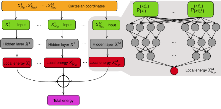
Figure 8: Deep potential net architecture.

III-A10 Deep Tensor Neural Networks

Recently, several researchers have exploited the DTNN capability to learn a multi-scale representation of the properties of molecules and materials from large-scale data in order to develop molecular and material simulators [89, 11, 105]. In more detail, DTNN initially recognizes and constructs a representation vector for each one of the atoms within the chemical environment, and then it employs a tensor construction algorithm that iteratively learns higher-order representations, after interacting with all pairwise neighbors.

Figure 9 presents a comprehensive example of DTNN architecture. The input, which consists of atom types and positions, is processed through several layers to produce atom-wise energies that are summed to a total energy. In the interaction layer, which is the most important one, atoms interact via continuous convolution functions. The variable $W^{t}$ stands for convolution weights that are returned from a filter generator function. Continuous convolutions are generated by DNNs that operate on interatomic distances, ensuring rototranslational invariance of the energy.

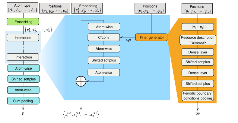
Figure 9: DTNN architecture.

DTNNs can accurately model a general QM molecular potential by training them in a diverse set of molecular energies [89]. Their main disadvantage is that they are unable to perform energy predictions for systems larger than those included in the training set [106].

III-A11 SchNet

SchNets can be considered as a special case of DTNN, since they both share atom embedding, interaction refinements and atom-wise energy contribution. Their main difference is that interactions in DTNNs are modeled by tensor layers, which provide atom representations. Parameter tensors are also used in order to combine the atom representations with inter-atomic distances [107]. On the other side, to model the interactions, SchNet employs filter convolutions, which are interpreted as a special case of computational-efficient low-rank factorized tensor layers [108, 109].

Conventional SchNets use discrete convolution filters (DCFs), which are designed for pixelated image processing in computer vision [110]. QM properties, like energy, are highly sensitive to position ambiguity. As a consequence, the accuracy of a model that discretize the particles position in a grid is questionable. To solve this problem, in [90], the authors employed continuous convolutions in order to map the rototranslationally invariant inter-atomic distances to filter values, which are used in the convolution.

III-A12 Accurate Neural Network Engine for Molecular Energies

Accurate neural network engine for molecular energies (ANAKIN-ME), or ANI for short, are networks that have been developed to break the walls built by DTNNs. The principle behind ANI is to develop modified symmetry functions (SmFs), which were introduced by BPNs, in order to develop NN potentials (NNPs). NNPs output single-atom atomic environments vectors (AEVs), as a molecular representation. AEVs allow energy prediction in complex chemical environments; thus, ANI solves the transferability problem of BPNs. By employing AEVs, the problem, which needs to be solved by ANI, is simplified into sampling statistically diverse set of molecular interactions within a predefined region of interest. To successfully solve this problem, a considerably large data set that spans molecular conformational and configurational space, is required. A trained ANI is capable of accurately predicting energies for molecules within the training set region [91].

As presented in Fig. 10, ANI uses the molecular coordinates and the atoms in order to compute the AEV of each atom. The AEV of atom $A_{i}$ (with $i=1,\cdots,N$), $\mathbf{G}_{A_{i}}$, scrutinizes specific regions of $A_{i}$’s radial and angular chemical environment. Each $\mathbf{G}_{A_{i}}$ is inputted in a single NPP, which returns the energy of atom $i$. Finally, the total energy of a molecule is evaluated as the sum of the energies of each one of the atoms.

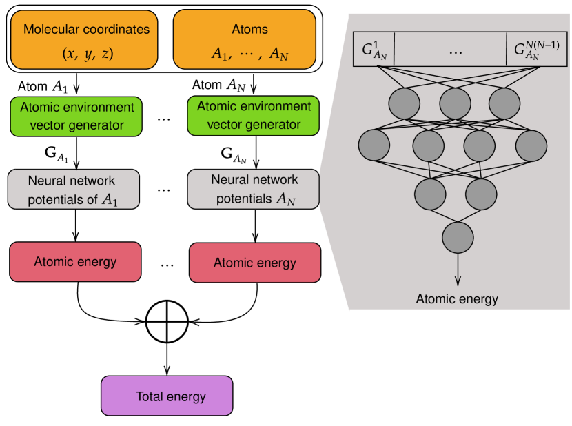
Figure 10: ANI architecture.

III-A13 Coarse Graining Networks

A common approach in order to go beyond the time and length scales, accessible with computational expensive molecular dynamics simulations, is the coarse-graining (CG) models. Towards this direction, several research works, including [111, 112, 113, 114, 115, 116, 117, 118, 119, 18], developed CG energy functions for large molecular systems, which take into account either the macroscopic properties or the structural features of atomistic models. All the aforementioned contributions agreed on the importance of incorporating the physical constraints of the system in order to develop a successful model. The training data are usually obtained through atomistic molecular dynamics simulations. Values within physically forbidden regions are not sampled and not included in the training. As a result, the machine is unable to perform predictions far away the training data, without additional constraints.

To countermeasure the aforementioned problem, CG networks employ regularization methods in order to enforce the correct asymptotic behavior of the energy when a nonphysical limit is violated. Similarly to BPNs and SchNets, CG networks initially translate the cartesian into internal coordinates, and use them to predict the rototranslationally invariant energy. Next, as illustrated in Fig. 11, the network learns the difference from a simple prior energy, which has been defined to have the correct asymptotic behavior [18]. Note that due to the fact that CG networks are capable of using available training data in order to correct the prior energy, its exact form is not required. Likewise, CG networks compute the gradient of the total free energy with respect to the input configuration in order to predict the conservative and rotation-equivariant force fields. The force-matching loss minimization of this prediction is used as a training rule of the CG network.

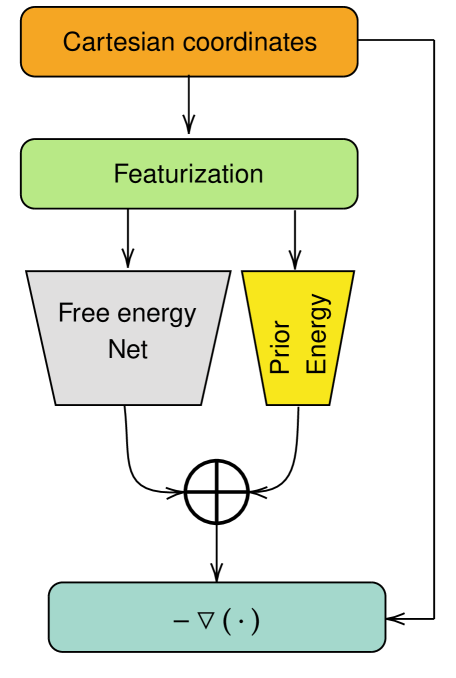
Figure 11: CG network architecture.

In practice, CGNs are used to predict the thermodynamic of chemical systems that are considerably larger than what is possible to simulate with atomistic resolution. Moreover, there have been recently presented some indications that they can also used to approximate the system kinetics, through the addition of fictitious particles [92] or by employing spectral matching to train the CGN [93].

III-A14 Neuromorphic Computing

Neuromorphic computing [103] is an emerging field, where the architecture of the brain is closely represented by the designed hardware-level system. The fundamental unit of neuromorphic computation is a memristor, which is a two-terminal device in which conductance is a function of the prior voltages in the device. Memristors were realized experimentally considering that many nanoscale materials exhibit memristive properties through ionic motion [120]. Nanophotonic systems are also utilized for neuromorphic computing and especially for the realization of deep learning networks [121] and adsorption-based photonic NNs [122].

Although neuromorphic computing and memristors tend to be a scalable practical technology, large area uniformity, reproducibility of the components, switching speed/efficiency and total lifetime in terms of cycles remain quite challenging aspects [123], which require either the development of novel memristive systems or improvements to existing systems. To this end, integration with existing complementary metal-oxide-semiconductor (CMOS) platforms and competitive performance advantage over CMOS neurons must be explored. These analog networks, after they are trained, can be highly efficient, however their training does not utilize digital logic and, thus, lacks flexibility [103].

III-B Regression

In this section, we discuss the regression methods that are commonly-used in the field of nano-scale biomedical engineering. Regression aims at characterizing the relationships among different variables. Three types of variables are identified in regression problems, namely predictors, objective, and distortion. A predictor, $x_{i}$, with $i\in[1,N]$, is an independent variable, while the objective, $Y$, is the dependent one. Moreover, let $d$ stand for the distortion parameter that model unknown parameters of the problem under investigation and affect the estimated value of the dependent parameter. Mathematically speaking, the objective of regression methods is to find the regression function $f\left(x_{1},\cdots,x_{N},d\right)$ that satisfies

$$Y=f\left(x_{1},\cdots,x_{N},d\right).$$ (9)

An important step for regression methods is to specify the form of the regression function. Based on the selected regression function, different regression methods can be identified. The rest of this section presents the regression methods that are commonly used in nano-scale biomedical engineering. In more detail, Section III-B1 provides a brief overview of logistic regression (LR), whereas Sections III-B2 and III-B3 respectively discuss multivariate linear regression (MvLR) and classification via regression. Finally, Sections III-B4 and III-B5 respectively report the operating principles of local weighted learning (LWL) and scoring functions (SFs). Table II summarizes the applications of regression methodologies in nano-scale biomedical engineering.

TABLE II: Regression applications in nano-scale biomedical engineering.

Paper	Application	Method	Description
[124]	Nanomedicine design	LR	Structure-activity relationships and design rules for spherical nucleic acids
[125]	Treatment design	LR	Classification of clinical trials based on an unsupervised ML algorithm
[126]	Chemical properties modeling	MvLR	Comparison of predictive computational models for nanoparticle
			induced cytotoxicity
[127]	Chemical properties modeling	Classification via Regression	Elimination of silico materials from potential human applications
[127]	Chemical properties modeling	LWL, SVM	Cytotoxicity prediction of NPs in biological systems
[128]	Chemical properties modeling	SF	Binding affinity and virtual screening prediction for nano-structures
[129]	Chemical properties modeling	SF	Quantification of the impact of protein structure on binding affinity

III-B1 Logistic Regression

LR is a supervised learning classification algorithm used to predict the probability of a target variable. The concept behind the target or the dependent variable is dichotomous, which means that there would be only two possible classes. LR can fit trends that are more complex than linear regression, but it still treats multiple properties as linearly related and is still a linear model. LR is named after the function used at the core of the method, the logistic function, which can take any real-valued number and map it into a value between $0$ and $1$. To provide a better understanding of LR, let us consider the binary classification problem in which $z$ is the dependent variable and $\mathbf{x}=[x_{1},x_{2},\cdots,x_{N}]$ are the $N$ independent variables. Since, for a fixed $\mathbf{x}$, $z$ follows a Bernoulli distribution, the probabilities $\Pr\left(z=1\left|\mathbf{x}\right.\right)$ and $\Pr\left(z=0\left|\mathbf{x}\right.\right)$ can be respectively obtained as

$$\Pr\left(z=1\left|\mathbf{x}\right.\right) =\frac{1}{1+\exp\left(-f(\mathbf{x})\right)},$$ (10)

$$\Pr\left(z=0\left|\mathbf{x}\right.\right) =1-\Pr\left(z=1\left|\mathbf{x}\right.\right)$$

$$=\frac{1}{1+\exp\left(f(\mathbf{x})\right)},$$ (11)

where

$$f(\mathbf{x})=c_{0}+\sum_{i=1}^{N}c_{i}x_{i},$$ (12)

with $c_{0},c_{1},\cdots,c_{N}$ being the regression coefficients. From (10), we can straightforwardly obtain $f(\mathbf{x})$ as

$$f(\mathbf{x})=\ln\left(\frac{\Pr\left(z=1\left|\mathbf{x}\right.\right)}{1-\Pr\left(z=1\left|\mathbf{x}\right.\right)}\right).$$ (13)

For a given training-set of length $N$, $\{z_{i},x_{i,1},\cdots,x_{i,M}\}$ with $i\in[1,N]$, the regression coefficients can be estimated by employing the maximum likelihood approach.

LR has been used extensively in biomedical applications, such as disease detection. Indicatively, in [124], LR was used to determine structure-activity relationships and design rules for spherical nucleic acids functioning as cancer-vaccine candidates. Moreover, in [125], it has been used for nano-medicine-based clinical trials classification and treatment development.

III-B2 Multivariate Linear Regression

Following the previous analysis, when multiple correlated dependent variables are predicted rather than a single scalar variable, the method is called MvLR. This method is a generalization of multiple linear regression and incorporates a number of different statistical models, such as analysis of variance (ANOVA), $t$-test, $F$-test, and more. MvLR has been used in ML for several nano-scale biomedical applications. Among the most successful ones is the prediction of cytotoxicity in NPs [126].

The MvLR model can be expressed in the form

$$y_{ik}=b_{0k}+\sum^{p}_{j=1}b_{jk}x_{ij}+e_{ik},$$ (14)

where $y_{ik}$ is the $k$-th response for the $i$-th observation, $b_{0k}$ is the regression intercept for the $k$-th response, $b_{jk}$ is the $j$-th predictor’s regression slope for the $k$-th response, $x_{ij}$ is the $j$-th predictor for the $i$-th observation, $e_{ik}$ is a Gaussian error term for the $k$-th response, $k\in\left[1,m\right]$ and $i\in\left[1,n\right]$.

III-B3 Classification via Regression

Conventionally, when dealing with discrete classes in ML, a classification method is used, while a regression method is applied, when dealing with continuous outputs. However, it is possible to perform classification through a regression method. The class is binarized and one regression model is built for each class value. In [127], in order to predict cytotoxicity of certain NPs, classification via regression is among the methods that were evaluated, in order to eliminate in silico materials from potential human applications.

III-B4 Local Weighted Learning

In the majority of learning methods, a global solution can be reached using the entirety of the training data. LWL offers an alternative approach at a much lower cost, by creating a local model, based on the neighboring data of a point of interest. In general, data points in the neighborhood of the point of interest, called query point, are assigned a weight based on a kernel function and their respective distance from the query point. The goal of the method is to find the regression coefficient that minimizes a cost function, similar to most regression methods. Due to its nature as a local approximation, LWL allows for easy addition of new training data. Depending on whether LWL stores in memory or not the entirely of the training data, LWL-based methods can be divided into memory-based and purely incremental, respectively [130].

Recently, LWL was used in [127], in order to predict the cytotoxicity of NPs in biological systems given an ensemble of attributes. It is found that when the data were further validated, the LWL classifier was the only one out of a set of classifiers that could offer predictions with high accuracy.

III-B5 Machine Learning Scoring Functions

SFs can be used to assess the docking performance, i.e. to predict how a small molecule binds to a target can be applied if a structural model of such target is available. However, despite the notable research efforts dedicated in the last years to improve the accuracy of SFs for structure-based binding affinity prediction, the achieved progress seems to be limited. ML-SFs have recently proposed to fill this performance gap. These are based on ML regression models without a predetermined functional form, and thus, are able to efficiently exploit a much larger amount of experimental data [128]. The concept behind ML-SFs is that the classical approach of using linear regression with a small number of expert-selected structural features can be strongly improved by using ML on nonlinear regression together with comprehensive data-driven feature selection (FS). Also, in [129] investigated whether the superiority of ML-SFs over classical SFs on average across targets, is exclusively due to the presence of training with highly similar proteins to those in the test set.

In Fig. 12 examples of classical and ML-SFs are depicted [128]. The first three (DOCK, PMF and X-SCORE) are classical SFs, which are distinguished by the employed structural descriptors. As it is evident, they all assume an additive functional form. On the other side, ML-SFs do not make assumptions about their functional form, which is inferred from the training data.

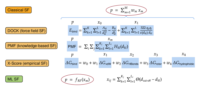
Figure 12: Examples of classical and ML-SFs (from [128])

III-C Support Vector Machine

NNs can be efficiently used in classification, when a huge number of data is available for training. However, in many cases this method outputs a local optimal solution instead of a global one. SVM is a supervised learning technique, which can overcome the shortcomings of NNs in classification and regression. For a brief but useful description of the SVM please see [131] and references therein. Next, for the help of the reader the SVM is summarized by using [131].

The aim of SVM is to find a classification criterion, which can effectively distinguish data at the testing stage. This criterion can be a line for two classes data, with a maximum distance of each class. This linear classifier is also known as an optimal hyperplane. In Fig. 13, the linear hyperplane is described for a set of training data, $\mathbf{x}=(1,2,3,...,n)$, as

$$\mathbf{w}^{T}\mathbf{x}+b=0,$$ (15)

where $\mathbf{w}$ is an n-dimensional vector and $b$ is a bias (error) term.

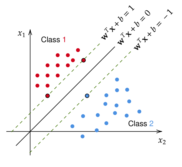
Figure 13: The SVM method [131]

This hyperplane should satisfy two specific properties: (1) the least possible error in data separation, and (2) the distance from the closest data of each class must be the maximum one. Under these conditions, data of each class can only belong to the left of the hyperplane. Therefore, two margins can be defined to ensure the separability of data as

$$\mathbf{w}^{T}\mathbf{x}+b\left\{\begin{array}[]{ll}\geq 1&\text{ for }y_{i}=1\\ \leq-1&\text{ for }y_{i}=-1\end{array}\right.$$ (16)

The general equation of the SVM for a linearly separable case, which would be subjected to two constraints as

$$\begin{array}[]{l}\operatorname{max}{L_{d}(\alpha)=\sum_{i=1}^{N}\alpha_{i}-\frac{1}{2}\sum_{i,j=1}^{N}y_{i}y_{j}\alpha_{i}\alpha_{j}x_{i}^{T}x_{j}}\\ \text{ s.t. }\left\{\begin{array}[]{l}\alpha_{i}\geq 0\\ \sum_{i=1}^{N}\alpha_{i}y_{i}=0\end{array}\right.\end{array}$$ (17)

where $\alpha$ is a Lagrange multiplier.

Eq. (17) is used in order to find the support vectors and their corresponding input data. The parameter $w$ of the hyperplane (decision function) can then be obtained as

$$w_{0}=\sum_{i=1}^{N}\alpha_{i}x_{i}y_{i}$$ (18)

and the bias parameter $b$ can be calculated as

$$b_{0}=\frac{1}{N}\sum_{S=1}^{N}\left(y_{S}-w^{T}x_{S}\right)$$ (19)

More details about the use of the linear as well as the non-linear SVM methods, can be found in [131].

An indicative training algorithm for SVM is the sequential minimal optimization (SMO). SMO is a training algorithm for SVMs. The training of an SVM requires the solution of a large quadratic programming (QP) optimization problem. Conventionally, the QP problem is solved by complex numerical methods, however SMO breaks down the problem into the smallest possible and solves it analytically, thus reducing significantly the amount of required time. SMO chooses two Lagrange multipliers to optimize, which can be done analytically, and updates the SVM accordingly. Interestingly, the smallest amount of Lagrange multipliers to solve the dual problem is two, one from a box constraint and one from linear constraint, meaning the minimum lies in a diagonal line segment. If only one multiplier was used in SMO, it would not be able to guarantee that the linear constraint is fulfilled at every step [132]. Moreover, SMO ensures convergence using Osuna’s theorem, since it is a special case of the Osuna algorithm, that is guaranteed to converge [133]. Recently, in [127], SMO was one of the classifiers used to predict cytotoxicity of Polyamidoamine (PAMAM) dendrimers, well documented NPs that have been proposed as suitable carriers of various bioactive agents.

SVM have been applied in many significant applications in bioinformatics and bioemedical engineering. Examples include: protein classification, detection of the splice sites, analysis of the gene expression, including gene selection for microarray data, where a special type of SVM called Potential SVM has been successfully used for analysis of brain tumor data set, lymphoma data set, and breast cancer data set ([134] and references therein).

Recently, SVM was considered in MCs. Specifically, in [135] the authors proposed injection velocity as a very promising modulation method in turbulent diffusion channels, which can be applied in several practical applications as in pollution monitoring, where inferring the pollutant ejection velocity may give an indication to the rate of underlying activities. In order to increase the reliability of inference, a time difference SVM technique was proposed to identify the initial velocities. It was shown that this can be achieved with very high accuracy.

In [136] a diffused molecular communication system model was proposed with the use a spherical transceiver and a trapezoidal container. The model was developed through SVM-Regression and other ML techniques, and it was shown that it performs with high accuracy, especially if long distance is assumed.

III-D $k-$Nearest Neighbors

KNN is a supervised ML classifier and regressor. It is based on the evaluation of the distance between the test data and the input and gives the prediction accordingly. The concept behind KNN is the classification of a class of data, based on the k nearest neighbors. Other names of this ML algorithm are memory-based classification and example-based classification or case-based classification.

KNN classification consists of two stages: the determination of the nearest neighbors and the class using those neighbors. A brief description of the KNN algorithms is as follows [137]: Let us considered a training data set $D$ consisted of $\left(\mathbf{x}_{i}\right)_{i\in[1,|D|]}$ training samples. The examples are described by a set of features $F$, which are normalized in the range$[0,1]$. Each training example is labelled with a class label $y_{j}\in Y$. The aim is to classify an unknown example $q$. To achieve this, for each $\mathbf{x}_{i}\in D$, we evaluate the distance between $q$ and $x_{i}$ as

$$d\left(\mathbf{q},\mathbf{x}_{i}\right)=\sum_{f\in F}w_{f}\delta\left(\mathbf{q}_{f},\mathbf{x}_{if}\right)$$ (20)

There are many choices for this distance metric; a fundamental metric, based on the Euclidian distance, for continuous and discrete attributes is

$$\delta\left(\mathbf{q}_{f},\mathbf{x}_{if}\right)=\left\{\begin{array}[]{ll}0&f\text{ discrete and }\mathbf{q}_{f}=\mathbf{x}_{if}\\ 1&f\text{ discrete and }\mathbf{q}_{f}\neq\mathbf{x}_{if}\\ \left|\mathbf{q}_{f}-\mathbf{x}_{if}\right|f&\text{ continuous }\end{array}\right.$$ (21)

The KNNs are selected based on this distance metric. There are a variety of ways in which the KNN can be used to determine the class of $q$. The most straightforward approach is to assign the majority class among the nearest neighbors to the query.

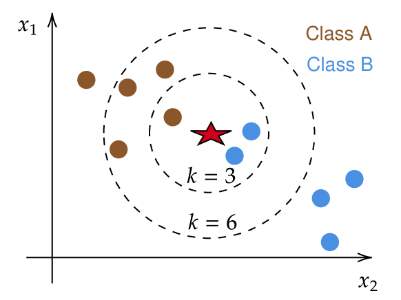
Figure 14: The KNN ML method.

Figure 14 depicts a $3$ and $6$ KNN on a two-class problem in a two-dimensional space [137]. The red star represents the test data point whose value is $(2,1,3)$. The test point is surrounded by yellow and blue dots which represent the two classes. The distance from our test point to each of the dots present on the graph. Since there are 10 dots, we get 10 distances. We determine the lowest distance and predict that it belongs to the same class of its nearest neighbor. If a yellow dot is the closest, we predict that our test data point is also a yellow dot. In some cases, you can also get two distances which exactly equal. Here, we take into consideration a third data point and calculate its distance from the test data. In Fig. 14 the test data lies in between the yellow and the blue dot. We considered the distance from the third data point and predicted that the test data is of the blue class.

The advantages of KNN are simple implementation and no need for prior assumption of the data. The disadvantage of KNN is the high prediction time.

III-E Dimentionality Reduction

This section is devoted to discussing dimentionality reduction methods. Dimentionality reduction constitutes the preparatory phase of ML, because the initially acquired raw data may contain some irrelevant or redundant features. Next, a comprehensive description of FS is provided in Section III-E1. Likewise, principal component analysis (PCA) and linear discriminant analysis (LDA) are respectively discussed in Sections III-E2 and III-E3. Finally, Section III-E4 presents the fundamentals of independent component analysis (ICA). Table III report the dimentionality reduction methodologies applications in nano-scale biomedical engineering.

TABLE III: Dimentionality reduction applications in nano-scale biomedical engineering.

Paper	Application	Method	Description
[138]	Disease detection	FS	Cancer prognosis and prediction
[139]	Disease detection	FS	Breast cancer detection
[140]	Disease detection	FS	Metastatic cancer detection
[141]	Disease detection	FS	Improved diagnoses based on composite biomarker signature
[142]	Image analysis	PCA	Spectroscopic image analysis
[143]	Signal analysis	PCA, LDA	Classification of EEG signals

III-E1 Feature Selection

FS reduces the complexity of a problem by detecting the subset of features that contribute most to the results. FS is one of the core concepts in ML, which hugely impacts the achievable performance. It is important to point out that FS is different from dimensionality reduction. Both methods seek to reduce the number of attributes in the data set, but a dimensionality reduction method do so by creating new combinations of attributes, whereas FS methods include and exclude attributes present in the data without changing them.

Combining ML algorithms with FS has been proven to be very useful for disease detection [138, 139]. It highlights the features associated with a specific target from a larger pool. For instance, in [140], a classification algorithm was used to analyze $10000$ genes from $200$ cancer patients, while FS was used to associate $50$ of them with metastatic prostate cancer. The selected features were then utilized as biomarker signature criteria in a ML algorithm for classification and diagnostics. Furthermore, recent research efforts provided evidence that combining data from multiple sources, such as transcriptomics and metabolomics to create composite signatures can improve the accuracy of biomarker signatures and disease diagnoses [141].

III-E2 Principal Component Analysis

PCA [142, 143, 103, 144] is an approach to solve the problem of blind source separation (BSS), which aims at the separation of a set of source signals from a set of mixed signals, with little information about the source signals or the mixing process. PCA utilizes the eigenvectors of the covariance matrix to determine which linear combinations of input variables contain the most information. It can also be used for feature extraction and dimensionality reduction. For cases with strong response variations, PCA allows an effective approach to rapidly process, de-noise, and compress data, however it cannot explicitly classify data.

More specifically, in PCA, the dimensional data are represented in a lower-dimensional space, reducing the degrees of freedom, the space and time complexities. PCA aims to represent the data in a space that best expresses the variation in a sum-squared error sense and is utilized for segmenting signals from multiple sources. As in standard clustering methods, it is useful if the number of the independent components is determined. Using the covariance matrix $\mathbf{C}=\mathbf{A}\mathbf{A}^{\mathrm{T}}$, where $\mathbf{A}$ denotes the matrix of all experimental data points, the eigenvectors $w_{k}$ and the corresponding eigenvalues $\lambda_{k}$ can be calculated. The eigenvectors are orthogonal and are chosen in order for the corresponding eigenvalues to be placed in descending order, i.e, $\lambda_{1}>\lambda_{2}>...$. To this end, the first eigenvector $w_{1}$ contains the most information and the amount of information decreases in the following eigenvectors. Therefore, the majority of the information is contained in a number of eigenvectors, whereas the remaining ones are dominated by noise.

III-E3 Linear Discriminant Analysis

LDA is another method for the solution of the BSS problem [143, 103]. In LDA, linear combinations of parameters that optimally classify data are identified and the main goal is to reduce the dimension of data. LDA has been used with a nanofluidic system to interpret gene expression data from exosomes and thus, to classify the disease state of patients. More specifically, LDA aims to create a new variable that is a combination of the original predictors, by maximizing the differences between the predefined groups with respect to the new variable. The predictor scores are utilized in order to form the discriminant score, which constitutes a single new composite variable. Therefore, the use of LDA results in an significant data dimension reduction technique that compresses the p-dimensional predictors into a one-dimensional line. Although at the end of the process the desired result is that each class will have a normal distribution of discriminant scores with the largest possible difference in mean scores between the classes, some overlap between the discriminant score distributions exists. The degree of this overlap represent a measure of the success of LDA. The discriminant function which is used to calculate the discriminant scores can be expressed as

$$D=w_{1}Z_{1}+w_{2}Z_{2}+...+w_{p}Z_{p},$$ (22)

where $w_{k}$ and $Z_{k}$ with $k=1,...p$ denote the weights and predictors, respectively. From (22), it can be observed that the discriminant score is a weighted linear combination of the predictors. The estimation of the weights aims to maximize the difference between each class mean discriminant scores. To this end, the predictors which are not similar with respect to the class mean discriminant scores will have larger weights, whereas the weights will reduce the more similar the class means are [145].

III-E4 Independent Component Analysis

ICA [143, 103, 144] was introduced in [146] and is another approach to the solution of the BSS problem. According to ICA, the original inputs are transformed into features, which are mutually independent and the non-orthogonal basis vectors that correspond to the correlations of the data are identified through higher order statistics. The use of the last one is needed, since the components are statistically independent, i.e., the joint PDF of the components is obtained as the product of the PDFs of all components.

Let consider $c$ independent scalar source signals $x_{k}(t)$, with $K=1,...,c$ and $t$ being a time index. The $c$ signals can be grouped into a zero mean.vector $x(t)$. Assuming that there is no noise and considering the independence of the components, the joint PDF can be expressed as

$$f_{x}(x)=\prod_{k=1}^{c}f_{x_{k}}(x_{k}).$$ (23)

An d-dimensional data vector, $y(t)$, can be observed at each moment through,

$$y(t)=Ax(t)$$ (24)

where $A$ is a $c\times d$ scalar matrix with $d\geq c$.

ICA aims to recover the source signals from the sensed signals, thus the real matrix $W=A^{-1}$ has to be determined. To this end, the determination of $A$ is performed by maximum-likelihood techniques. An estimate of the density, termed as $\hat{f}_{y}(y;a)$, is used and the parameter vector $a$, that minimizes the difference between the source distribution and the estimate has to be determined. It should be highlighted that $a$ is the basis vector of $A$ and, thus, $\hat{f}_{y}(y;a)$ is an estimate of $f_{y}(y)$.

III-F Gradient Descent Method

When there are one or more inputs the optimization of the coefficients by iteratively minimizing the error of the model on the training data becomes a very important procedure. This operation is called GD and initiates with random values for each coefficient. The sum of the squared errors is calculated for each pair of input and output values. A learning rate is used as a scale factor and the coefficients are updated to minimize the error. The process is repeated until a minimum sum squared error is achieved or no further improvement is possible. In practice, GD is taught using a linear regression model due to its straightforward nature and it proves to be useful for very large datasets [147].

GD is one of the most popular algorithms to optimize in NNs and has been extensively used in nano-scale biomedical engineering. For example, in [29], the authors proposed a method to use ANNs to approximate light scattering by multi-layer NPs and used the GD for optimizing the input parameters of the NN.

III-G Active Learning

In AL, also known as the optimal design of experiments, a surrogate model is created from a given data set, and then the model is used to select which data should be obtained next [148]. The selected data are added to the original data set and then used to create an updated surrogate model. The process is repeated iteratively such that the surrogate model is improved continuously. In contrast to classic ML methods, the identifier of an AL system is that it develops and tests new hypotheses as part of a continuing, interactive learning process. This method of iterative surrogate model screening has already been used in other fields, such as drug discovery and molecular property prediction [149, 150].

III-H Bayesian Machine Learning

In addition to the Bayes Theorem is a powerful tool in statistics, it is also widely used in ML to develop models for classification, such as the Optimal Bayes classifier and Naive Bayes. The optimal Bayes classifier selects the class that presents the largest a posteriori probability of occurrence. It can be shown, that among all classifiers, the Optimal Bayes classifier has the lowest error probability. In most real-life applications the posterior distribution is unknown but can rather be estimated. In this case, the Naive Bayes classifier approximates the optimal Bayes classifier by looking at the empirical distribution and assuming independence of predictors. So, the Naive Bayes classifier is a simple but suboptimal solution. It should be mentioned that Naive Bayes can be coupled with a variety of methods to improve the accuracy [151]. Furthermore, since it relies on the computation of closed-form expressions of a posteriori probabilities, it takes linear time to compute, in contrast to expensive iterative approximations that are commonly used in other methods.

Assuming an instance that is represented by the observation of $n$ features, $\mathbf{x}=(x_{1},\dots,x_{n})$, Naive Bayes assigns a probability $p(C_{k}|\mathbf{x})$ for each possible class $C_{k}$ among $K$ possible outcomes. According to Bayes’ theorem, the posterior probability is given by the prior times the likelihood over the evidence, i.e.

$$p(C_{k}|\mathbf{x})=\frac{p(C_{k})p(\mathbf{x}|C_{k})}{p(\mathbf{x})}.$$ (25)

The evidence is not dependent on $C$ so it is of no interest. Naive Bayes is a naive classifier because it assumes that all features in $\mathbf{x}$ are mutually independent conditioned on $C_{k}$. Therefore, it assigns a class label as

$$\hat{y}=\underset{k\in\{1,\dots,K\}}{\mathrm{argmax}}p(C_{k})\prod_{i=1}^{n}p(x_{i}|C_{k}).$$ (26)

Bayesian analysis and ML are playing an important role in various aspects of nanotechnology and related molecular-scale research. Recently it has been shown that an atomic version of Green’s function and Bayesian optimization is capable of optimizing the interfacial thermal conductance of Si-Si and Si-Ge nano-structures [152]. This method was able to identify the optimal structures between $60000$ candidate structures. Furthermore, more recent works have relaxed the data requirement limitations by adapting output parameters to unsupervised learning methods such as Bayesian statistical methods that do not rely on an external reference [153, 154, 155]. Naive Bayes has been applied to predict cytotoxicity of PAMAM dendrimers, which are well documented NPs that have been proposed as suitable carriers of various bioactive agents, in [127]. By pre-processing the data, Naive Bayes presented substantial improvement in the accuracy despite its simplicity, thus, outperforming the classification methods used in [127].

III-I Decision Tree Learning

DTL is a predictive modeling technique used in ML, which uses a decision tree to draw conclusions about the target value based on observations. In the tree paradigm, the target values are represented as leaves, while the observations are denoted by branches. There are two types of DTL, namely classification and regression trees. In the former, the target variable belongs in a discrete set of values, while in the latter the target variable is continuous. Furthermore, some techniques, such as bagged trees and bootstrap aggregated decision trees, use multiple decision trees. In more detail, the bagged trees method builds an ensemble incrementally by training each new instance to emphasize the training instances that were previously mis-modeled. The bootstrap aggregated decision trees is an early ensemble method that creates multiple decision trees by resampling training data and voting the trees for a consensus prediction.

DTL has been used extensively in nano-medicine by optimizing material properties according to predicted interactions with the target drug, biological fluids, immune system, vasculature, and cell membranes, all affecting therapeutic efficacy [156]. Specifically, in [157], decision trees were used for classification of effective and ineffective sequences for Ribonucleic acid interference (RNAi) in order to recognize key features in their design. In addition, several algorithms have been developed over the years that improve the accuracy and efficiency of DTL. For instance, the J48 algorithm is considered among the best algorithms with regards to accuracy and has been used in various biomedical tasks, such as predicting cytotoxicity, measured as cell viability [158, 127].

Next, we present the most commonly used DTL methods. In this direction, Bootstrap aggregating (bagging) is revisited in Section III-I1, while the operating principles of bagged trees are highlighted in Section III-I2. Moreover, the fundamentals of bagged Bayes trees are discussed in Section III-I3, whereas the adaptive boosting (AdaBoost) approach is reported in Section III-I4. Finally, descriptions of random forest (RForest) and M5P approaches are respectively delivered in Sections III-I5 and III-I6

TABLE IV: Decision tree learning applications in nano-scale biomedical engineering.

Paper	Application	Method	Description
[156]	Disease treatment	DTL	Cancer treatment
[157]	Chemical properties modeling	DTL	Feature recognition in the design of RNA sequences
[158]	Chemical properties modeling	DTL	Prediction of cytotoxicity
[127]	Chemical properties modeling	DTL, NBTree	Prediction of cytotoxicity
[159]	Chemical properties modeling	Bagging, M5P	Prediction of cytotoxicity
[160]	Disease prediction	Bagged tree, AdaBoost	Heart disease prediction
[161]	Disease detection	AdaBoost	Particle detection in cryo-electon micrographs
[162]	Chemical properties modeling	AdaBoost	Characterization nanomaterial properties

III-I1 Bagging

Bootstrapping methods have been used extensively to minimize statistical errors of predictors by utilizing random sampling with replacement. In supervised learning, a training dataset is utilized to train a predictor. Bootstrap replicas of the training dataset can be employed to generate new predictors. bagging is a meta-learning algorithm that uses this idea to develop an aggregated predictor, either by averaging the predictors over the learning sets when the exit is numerical or by voting, when the exit is a class label [163]. More specifically, assuming a learning set $\mathcal{L}$ consists of data $\{(y_{n},\mathbf{x}_{n}),n=1,\dots,N\}$ and a predictor $\phi(\mathbf{x},\mathcal{L})$, $y$ is predicted by $\phi(\mathbf{x},\mathcal{L})$ if the input is $\mathbf{x}$. The learning set consists of $N$ observations and since it is hard or in many cases impossible to obtain more observations to improve the learning set, we turn to bootstrapping, creating different learning sets using the sample $N$ as the population, which effectively leads to new predictors ($\{\phi(\mathbf{x},\mathcal{L})\}$). The aggregated predictor’s accuracy is determined by the stability of the procedure for constructing each $\phi$ predictor, i.e., the accuracy will be improved with bagging in unstable procedures, where small variation in the learning set leads to large changes in the predictor.

Recently, bagging has been used to predict possible toxic effects caused by the exposure to nanomaterials in biological systems [159]. As a base predictor $\phi$, REPTree was used, which is a fast decision tree-based learning algorithm. It should be mentioned that the bagging algorithm offered the highest accuracy, in terms of correlation, between actual and predicted results.

III-I2 Bagged Tree

Bagging can be applied to any kind of model. By using bagged decision trees, it is possible to lower the bias by leaving the trees un-pruned. High variance and low bias is essential for bagging classifiers. The aggregate classifier can capitalize on this and provide an increase in accuracy. In [160], a bagged tree was used with great success in a ensemble classifier with particle swarm optimization (PSO) in order to predict heart disease.

III-I3 Naive Bayes Tree

A hybrid approach to learning, when many attributes are deemed relevant for a classification task, yet they are not sufficiently independent, is the NBTree. NBTree consists in practice of a decision tree with Naive Bayes classifiers at the leaf nodes [164]. Firstly, according to a utility function an attribute is split in the decision tree making process. If the utility is not sufficiently high, the node becomes a leaf and a Naive Bayes classifier is created at the node. NBTree can deal both with discrete data, by multi-way splits for all values, and with continuous data, by using a threshold split.

In [127], NBTree was used among other learning methods as a way to predict the cytotoxicity of nanomaterials in biological systems. When leave-one-out cross validation was performed, NBTree achieved the best performence and achieved an accuracy of $77.7\%$.

III-I4 Adaptive Boosting

AdaBoost is a learning method that uses an ensemble of classifiers in order to improve accuracy [165, 166]. Boosting is a technique that takes a set of weak learners –usually a decision tree classifier– and combines them into a strong one. The procedure can be summarized as follows. A set of labeled training examples $\{(x_{i},y_{i})\}$, where $x_{i}$ is an observable quality and $y_{i}$ is the outcome, are given into a set of classifiers that are each assigned a weight. After every weak classifier has reached to a prediction, the boosting method combines all the weak hypotheses into a single prediction. AdaBoost does not need prior knowledge of the accuracies of the weak classifiers, instead, it adapts to the errors of the weak classifiers. In essence, the weak classifiers are tweaked to better handle data that were mishandled by previous classifiers. In some cases, AdaBoost has shown to be less susceptible to over-fitting than other learning methods, however it is prone to noisy data and outliers due to its adaptive nature.

AdaBoost was one of the methods used in [160] in an ensemble classifier together with PSO to predict heart disease. Moreover, AdaBoost was used in [161] as a learning approach for particle detection in cryo-electron micrographs. Similarly, in [162], it was used for characterizing and analyzing unique features and properties of nanomaterials and nanostructures.

III-I5 Random Forest

RForest is one of the one of the most used ML algorithms, due to its simplicity and diversity, since it can be used for both classification and regression. As the name suggests, a RForest is a tree-based ensemble, where each tree is connected to a collection of random variables [167]. In Fig. 15, RForest average multiple decision trees are presented, that have been trained on different parts of the same training set, in order to reduce the variance. The different decision trees are trained based on the bagging technique, thus they exploit the random subsets of the training data. An advantage of RForest is that it decreases the variance of the model and, thus, combines uncorrelated individual trees with bagging, making them more robust without increasing the bias to overfitting. Another technique for combining individual trees is boosting, where the samples are weighted for sampling so that samples, which were predicted incorrectly, get a higher weight and are therefore, sampled more often. The concept behind this is that difficult cases should be emphasized during learning, compared to easy ones. Because of this difference, bagging can be easily paralleled, while boosting is performed sequentially. Next, we provide briefly the mathematical concept behind the RForest method.

Figure 15: Random forest diagram.

We assume an unknown joint distribution $P_{XY(X,Y)}$, where $X=\left(X_{1},\ldots,X_{p}\right)^{T}$ is a $p$-dimensional random vector, which represents the predictor variables and $Y$ is the real-valued response. The aim of the RForest algorithm is to find a prediction function $f(X)$ in order to predict $Y$. The prediction function is that which minimizes the expected value of the loss function $L(Y,f(X))$, i.e. $E_{XY}(L(Y,f(X))),$ where the subscripts denote expectation with respect to the joint distribution of $X$ and $Y$.

Note that $L(Y,f(X))$ is a measure of how close $f(X)$ is to $Y$ and it penalizes values of $f(X)$ that are far from $Y$. Typical choices of $L$ are squared error loss $L(Y,f(X))=(Y-f(X))^{2}$ for regression and zero-one loss for classification:

$$L(Y,f(X))=I(Y\neq f(X))=\left\{\begin{array}[]{l}0\text{ if }Y=f(X)\\ 1\text{ otherwise. }\end{array}\right.$$ (27)

It turns out that minimizing $E_{XY}(L(Y,f(X)))$ for squared error loss gives the conditional expectation $f(x)=E(Y\mid X=x)$, which is known as the regression function. When classification is considered, if the set of possible values of $Y$ is denoted by $\mathcal{Y}$, then minimizing $E_{XY}(L(Y,f(X)))$ for zero-one loss results to

$$f(x)=\arg\max_{y\in\mathcal{Y}}P(Y=y\mid X=x)$$ (28)

which is the Bayes rule.

Ensembles construct $f$ in terms of the so-called “base learners” $h_{1}(x),...,h_{J}(x)$ and these are combined to give the “ensemble predictor” $f(x)$. In regression, the base learners are averaged

$$f(x)=\frac{1}{J}\sum_{j=1}^{J}h_{j}(x)$$ (29)

while in classification, $f(x)$ is the most frequently predicted class

$$f(x)=\arg\max_{y\in\mathcal{Y}}\sum_{j=1}^{J}I\left(y=h_{j}(x)\right)$$ (30)

In RForests the $j_{th}$ base learner is a tree denoted as $h_{j}\left(X,\Theta_{j}\right)$, where $\Theta_{j},j=1,...,J.$ is a collection of independent random variables. To deeply understand the RForest algorithm, a fundamental knowledge of the type of trees used as base learners is needed.

III-I6 M5P

The M5 model tree method was introduced by Quinlan in $1992$ [168]. Wang and Witten later presented an improved public-domain scheme [169], called M5P, that generates more compact and comprehensible models with slightly better accuracy. M5P combines conventional binary decision tree models with regression planes at the leaves, to provide a way to deal with continuous-class problems. The initial tree split is based on a standard deviation criterion, called standard deviation reduction (SDR) and given by

$$\mathrm{SDR}=\mathrm{SD}(A)-\sum_{i}\frac{|T_{i}|}{|T|}\mathrm{SD}(T),$$ (31)

where $\mathrm{SD}(A)$ is the standard deviation of the set $A$, $T$ is the set of learning examples that reach the node, and $\{T_{i}\}$ are the subsets that result from splitting $T$ according to a chosen attribute. The attribute that maximizes SDR is the chosen for the split. However, this process can lead to large tree structures that are prone to over-fitting. Therefore, pruning the tree is necessary to improve accuracy. For every interior node of the tree, a regression model is calculated with the examples that reach that node, if the subtree error is greater than the respective error of the regression model in that node, the tree is pruned and that particular node is turned into a leaf node.

Recently, M5P was used in [159] to built a simulator that can dynamically predict the mortality rate of cells in biological systems in order to test possible toxic effects from exposure to nano-materials. The simulator’s user can change the attribute values dynamically and obtain the predicted value of the used metric.

III-J Decision Table

A DT is a simple tabular representation of conditions and actions [170]. It is very similar to the popular decision trees. A key difference between among them is that the former can include more than one “OR” condition. However, DTs are usually preferred when a small number of features is available, whereas decision trees can be used for more complex models.

Decision Table Naive Bayes

Combined learning models is an efficient way to improve the accuracy of stand-alone models. DT Naive Bayes (DTNB) is such a hybrid model, where a DT classifier is combined with a naive Bayes network, to produce a table with conditional probabilities. The learning process for DTNB splits the training data into two disjoint subsets and utilizes one set for training the DT and the other for training the NB [170]. The goal is to use NB on the attributes that are somewhat independent, since NB already assumed independence of attributes. Cross validation methods are suitable in this hybrid model since it is effective in both DTs, due to the structure of the table remaining the same, and the NB as the frequency counts can be updated in constant time.

Assuming that $\mathbf{x}^{\mathrm{DT}}$ is the set of attributes used in DT, and $\mathbf{x}^{\mathrm{NB}}$ is the respective set of attributes for NB, the class $k$ probability can be computed as

$$P(C_{k}|\mathbf{x})=\frac{aP(C_{k}|\mathbf{x}^{\mathrm{DT}})P(C_{k}|\mathbf{x}^{\mathrm{NB}})}{P(C_{k})},$$ (32)

where $a$ is a normalization constant and $P(C_{k})$ is the prior probability of the class. DTNB is shown to achieve significant gains over both DTs and NB. More specifically, in [127], DTNB was used among other methods to predict cytotoxicity values of nanomaterials in biological systems.

III-K Surrogate-Based Optimization

Surrogate-based optimization [171, 172] refers to a class of optimization methodologies, that calculate the local or global optima by utilizing surrogate modeling techniques. This framework utilizes conventional optimization algorithms, such as gradient-based or evolutionary algorithms, for sub-optimization. Surrogate modeling techniques can significantly improve the design efficiency and facilitate finding global optima, filtering numerical noise, accomplishing parallel design optimization and integrating simulation codes of different disciplines into a process chain.

In optimization problems, surrogate models can approximate the cost functions and the state functions, constructed from sampled data which are obtained by randomly exploring the design space. After this step, a new design based on the surrogate models, which is most likely to be the optimum, is searched by applying an optimization algorithm such as Genetic Algorithms. Utilizing a surrogate model for the estimation of the optimum is more effective than using a numerical analysis code, thus, the computational cost of the search based on the surrogate models is negligible. Surrogate models are built from the sampled data, thus the way the sample points are chosen and the way the accuracy of surrogate models is evaluated are important issues for surrogate modeling.

In [173], surrogate-based optimization is used to search the space of intermetallics for potentially selective catalysts for $\text{CO}_{2}$ reduction reaction and hydrogen evolution reaction.

III-L Quantitative Structure-Activity Relationships

ML techniques have been combined with QSARs models over the past decade [174]. One of the most successful applications of such models is the development of new drugs faster and with lower cost. QSAR methods are data-driven and based on supervised learning. They capture the complex relationships between the properties of nanomaterials without requiring detailed knowledge of the mechanisms of interaction. In more detail, every biological activity of organic molecules is a function of their structural properties that depend on their chemical structures. These relationships can be expressed as in [174]

$$\text{Activity}=f\left(\sum\left(\text{Properties}\right)\right),$$ (33)

and

$$\text{Property}=f\left(\text{Structure}\right).$$ (34)

Due to the complexity of the materials the predictivity of the applied methods must be optimized, thus various different techniques have been used in the literature. Specifically, in [175], QSAR models were developed based on sparse linear FS and regression in conjunction with a minimization algorithm, while, in [176, 177, 178], nonlinear FS was used with Bayesian regularized NNs that used Gaussian or Laplacian priors. Also, ANNs have been recently employed to forecast the biological activity of compounds under investigation, while the ANN-classification model categorizes the compounds for a specific biological response [179].

III-M Boltzmann Generator

The aim of statistical mechanics is to assess the average behavior of physical systems based on their microscopic constituents and interactions, in order not only to understand the molecules and materials functionalities, but also provide the principles for devising drug molecules and materials with novel properties. In this direction, the statistics of the equilibrium states of many-body systems needs to be evaluated. To conceive the complexity of this, let us try to evaluate the probability that, at a given temperature, a protein will be folded. In order to solve this problem, we need to examine each one of the huge number of ways to place all the proteins in a predetermined space and for each one of them extract the corresponding probability. However, since the enumeration of all configurations is extremely difficult or even infeasible, the necessity to sample them from their equilibrium distribution has been identified in  [28]. In this work, the authors proposed the Boltzmann generator, which combines deep ML and statistical mechanics in order to learn sample equilibrium distributions. In contrast to conventional generative learning, the Boltzmann generator is not trained to learn the probability density from data, but to directly produce independent samples of low-energy structures for condensed-matter systems and protein molecules.

As presented in Fig. 16, the operation principle of Boltzmann generator consists of two parts:

1. A generative model, $F_{zx}$, is trained capable of providing samples from a stochastic distribution, which is described by the probability density function (PDF), $f_{x}(x)$, when sampling $z$ from a simple prior, such as a Gaussian distribution with PDF $f_{z}(z)$.

2. A re-weighting process that transforms the generated distribution, $f_{x}(x)$, into the Boltzmann distribution, and produces unbiased samples from the $e^{-u(x)}$, with $u(x)$ being the dimensionless energy.

Note that both training and re-weighting require $f_{x}(x)$ knowledge. This can be ensured by adopting an invertible $F_{zx}$ transformation, which allows us to transform $f_{z}(z)$ to $f_{x}(x)$.

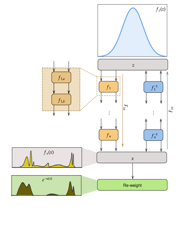
Figure 16: Boltzmann generator.

III-N Feedback System Control

FSC [180] is a recently proposed method for the optimization of drug combinations. FSC is a phenotypically driven optimization process, which does not require any mechanistic knowledge for the system. This is the reason that FSC can be successfully applied in various complex biological systems (see [181] and references therein)

The FSC method is based on the closed-loop feedback control process outlined in Fig. 17 [180]. It mainly consists of two steps: the first step is the definition of an initial set of compounds to be tested. The second step refers to the generation of broad dose-response curves for each compound in the selected cellular bioassay, which is selected to provide a phenotypic output response, that is used to evaluate the efficacy of the drugs and drug combinations on overall cell activity.

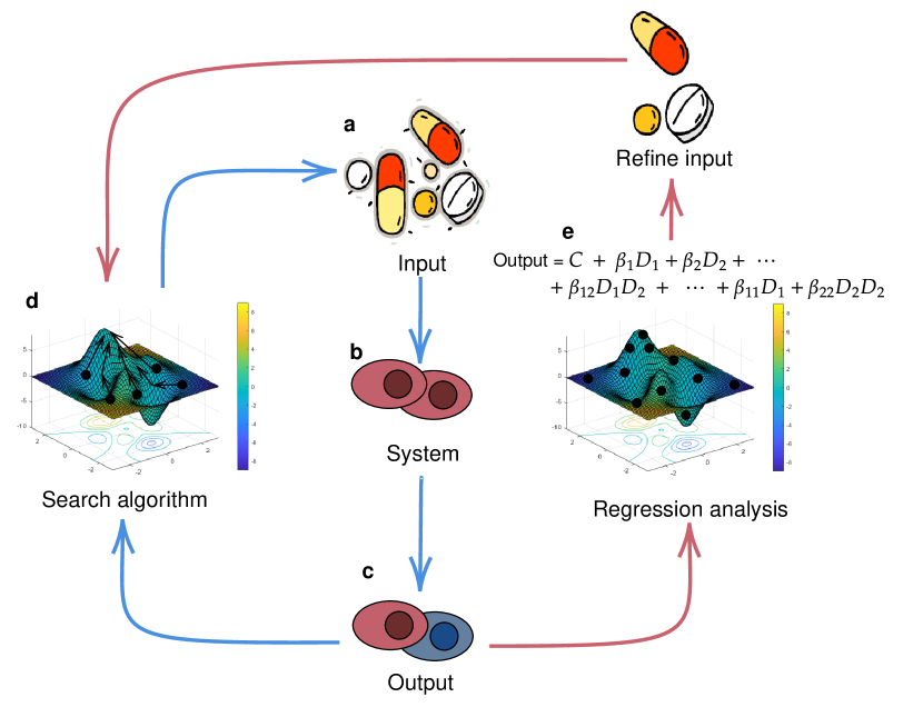
Figure 17: Examples of classical and ML-SFs.

A schematic representation of the FSC technique is presented in Fig. 17. The five main components of the optimization process are depicted as:

(a) The input, i.e., the drug combinations with defined drug doses.

(b) The system, i.e., the selected cell type representation of the disease to be studied

(c) The system output, i.e., the cellular response to the defined drug combination input in the selected cell bioassay.

(d) The search algorithm that iteratively drives the system output toward the desired response.

(e) The statistical analysis used to guide drug elimination.

III-O Quadratic Phenotypic Optimization Platform

Methods based on ML, like FSC, aim to overcome the disadvantages of the traditional methods, as for example the high-throughput screening. Recently, a powerful AI platform called Quadratic Phenotypic Optimization Platform (QPOP) was proposed, to interrogate a large pool of potential drugs and to design a novel combination therapy against multiple myeloma [69]. This platform can efficiently and iteratively outputs effective drug combinations and can optimize the drug doses.

The main concept of QPOP lies in recognizing the relationship between inputs (e.g., drugs) and desired phenotypic outputs (e.g., cell viabilities) to a smooth, second-order quadratic surface representative of the biological system of interest. Since QPOP utilizes only the controllable inputs and measurable phenotypic outputs of the biological system, it is able to identify optimal drug combinations and doses independently of predetermined drug synergy information and pharmacokinetic properties. Furthermore, QPOP utilized ML in order to preclinically re-optimize the combination and successfully translate the multi-drug regimen through in vivo validation. It is important to mention that both the in vitro and preclinical re-optimization processes were able to simultaneously take into account both efficacy and safety, and this is an important aspect of the QPOP platform.

QPOP can also be used as an actionable platform to design patient-specific regimens. This multi-parametric global optimization methodology can overcome many of the drug development process difficulties, and can result in efficient and safe therapies. This will revisit the drug development, translating into improved and effective treatment choices.

More details about the use of the QPQP platform in biomedicine applications can be found in [182] and [183] and references therein.

IV Discussion & The Road Ahead

In this section, we clarify how the ML methodologies presented in Section III can be efficiently used to solve the problems discussed in Section II and elaborate on some major open research problems, which are of great importance for unveiling the potential benefits, advantages, and limitations of employing ML in nano-scale biomedical engineering. In this direction, Table V, which is given in the top of the next page, connects the ML challenges with the ML methodologies, that have been used in nano-scale biomedical engineering.

TABLE V: ML problems and solutions.

ML approaches	ML challenge categories
	Structure and material design and simulation	Communications and signal processing	Applications
ANNs
Convolution neural networks	✓	✓	✓
Recurrent neural networks	✓	✓	✓
Deep neural networks	✓	✓	✓
Diffractive deep neural networks	✓	-	-
Generalized regression neural networks	✓	-	✓
Multi-layer perceptron	✓	✓	-
Generative adversarial networks	✓	-	✓
Behler-Parrinello networks	✓	-	-
Deep potential networks	✓	-	-
Deep tensor neural networks	✓	-	-
SchNet	✓	-	-
Accurate neural network engine for molecular energies	✓	-	-
Coarse graining	✓	-	-
Neuromorphic computing	✓	-	-
Regression
Logistic regression	✓	✓	✓
Multivariate linear regression	✓	-	-
Classification via regression	✓	-	-
Local weighted learning	✓	-	-
Machine learning scoring functions	✓	-	-
Support vector machine
Support vector machine	✓	✓	✓
$k$-nearest neighbors
$k$-nearest neighbors	✓	✓	-
Dimentionality reduction
Feature selection	✓	-	-
Principle component analysis	✓	-	✓
Linear discriminant analysis	✓	-	✓
Independent component analysis	✓	-	✓
Gradient descent
Gradient descent	✓	-	-
Active learning
Active learning	✓	-	-
Bayesian ML	✓	✓	✓
Decision tree learning
Bagging	✓	✓	-
Bagged tree	-	-	✓
Naive Bayer tree	✓	-	✓
Adaptive boosting	-	-	✓
Random forest	-	-	✓
M5P	✓	-	-
Decision table
Decision table naive Bayes	✓	✓	-
Surrogate-based optimization
Surrogate-based optimization	✓	-	-
QSAR
QSAR	✓	-	✓
Boltzmann generator
Boltzmann generator	✓	-	-
Feedback system control
Feedback system control	-	-	✓
Quadratic phenotypic optimization platform
Quadratic phenotypic optimization platform	✓	-	✓

From Table V, it becomes evident that ANNs can be employed to solve a large variety of ML problems in nano-scale biomedical engineering. The ML methods CNNs, RNNs, and DNNs are capable of identifying patterns, locate and classify target objects in an image, and detect events [184]. As a result, they can excel in the development of ARES, which contributes to the discovery, design, and performance optimization of nano-structures and nano-materials. Furthermore, they can be used for the detection of received symbols in molecular and electromagnetic nano-networks, for the classification of observations that may provide a better understanding of biological and chemical processes, and for the identification of specific patterns. On the other hand, D²NNs can efficiently execute identification and classification tasks, after being trained by large datasets. Therefore, they have been successfully used in lens imaging at THz spectrum, while they are expected to find application in image analysis, feature detection, and object classification. In other words, D²NNs may be employed for heterogeneous nano-structures discovery, channel estimation and symbol detection in nano-scale molecular and THz networks, as well as disease detection and therapy development.

By inducing the algorithm to learn complex relationships within a training dataset and making judgments on test datasets with high fidelity, GRNNs are capable of providing a systematic methodology to map inputs to predictive outputs. As a consequence, they have been applied in several fields, including optical character recognition, pattern recognition, and manufacturing for predicting the output classification [185, 186]. In nano-scale biomedical engineering, they have been extensively used in discovering the properties of and designing heterogeneous nano-structures [186, 187] as well as analyzing the data collected from them [188]. However, their applicability in molecular and electromagnetic nano-scale networks specific problems needs to be assessed.

Based on Cybernko’s theorem [189], MLPs are proven to be universal function approximators. In other words, they return low-complexity approximating solutions from extremely complex problems. As a result, MLPs have been a popular ML method in 80s in several fields including speech and image recognition (see e.g., [190, 191] and references therein). In nano-scale biomedical engineering, MLPs have been applied for nano-structure properties discovery [192, 193] and data analysis [80]. However, it is expected to be replaced by much simpler SVMs, which are considered their main competitors.

GANs have been recently used to inversely design metasurfaces in order to provide arbitrary patterns of the unit cell structure [194]. However, they experience high instability. To solve this problem conditional deep convolutional GANs are usually employed. These networks return very stable Nash equilibrium solutions that can be used for inversely designing nanophotonic structures [84, 195]. Another application of GANs lies in the statistical characterization of psychological wellness states [80]. In general, for applications in which the data have a non-linear behavior, GANs achieve similar performance as SVMs and $k-$nearest neighbor, and outperform MLPs.

Classical force field theory can neither easily scale into large molecules nor become transferable to different environments. To break these limitations, BPMs, DPNs, DTNNs, SchNets, and CGNs have been traditionally used to model the PESs and atomic forces in large molecules, like proteins and provide transferability to different covalent and non-covalent environments. However, these approaches are incapable of reaching the required accuracy with lower than classical force field evaluation complexity. Motivated by this, symmetrized gradient-domain ML have been very recently presented as a possible solution to the aforementioned problem [14, 196, 197, 198]. The limitation of this ML approach is that it cannot support molecules that consists of more than $20$ atoms. In other words, it lacks scalability and transferability. To countermeasure this, researchers should turn their eye in combining BPMs, DPNs, DTNNs, SchNets, and CGNs with gradient-domain ML in order to provide high-accuracy in configuration and chemical space simulations. A plethora of new insights awaits as a result of such simulations.

Regression approaches have been used to extract the relationship between several independent variables and one dependent variable. Therefore, they have supported the solution of a large variety of problems that range from the area of nano-materials and nano-structure design to data-driven applications in biomedical engineering [124, 136]. Moreover, they usually require no input features or tuning for scaling and they are easy to regularize. However, it is incapable of solving non-linear problems. Another disadvantage of regression approaches is that they require the identification of all the important independent attributes before inserting the data into the machine. Moreover, most of them return discrete outputs, i.e., they only provide categorical outcomes. Finally, they are sensitive to overfitting [199].

Similarly to regression, SVMs are efficient methods for problems with high-dimensional spaces. Taking this into account, several researchers have adopted them in order to provide solutions to a large range of problems from heterogeneous structure design to signal detection in molecular communication systems and data-driven applications. However, as the data set size increases, SVMs may underperform. Another limitation that should be highlighted is that they are not suitable for problems with overlapping targeting classes [200].

KNN has been employed in structure and material design [201], MCs for symbol detection [6], and disease detection [202, 203]. It is a low-complexity approach suitable for classifying data without training. However, it suffers from performance degradation when applied to large data sets, due to increased cost of computing the distance between the new point and each of the existing points. A similar performance degradation is observed as the dimensions of the data increase. This indicates that the application of KNN approach in heterogeneous nano-structure design is questionable. On the other hand, it excels in data sequence detection in MC systems, where the dimension of the data is no higher than $2$.

Dimensionality reduction methods have been applied in the nano-structure and material design [204, 205] as well as in therapy development [206]. Their objective is to remove dimensions, i.e. redundant features, in order to identify the more suitable variable for the problem under investigation. As a result, they contribute to data compression and to computation time reduction. Moreover, they are capable of transforming multi-dimensional problems into two dimensional (2D) or 3D ones allowing their visualization. This property has been extensively used in nano-structure properties discovery. Likewise, dimensionality reduction methods can aid at noise removal; thus, they can significantly improve the model’s performance. However, they come with some disadvantages. In particular, they cause data loss. Moreover, PCA tends to extract linear correlations between variables. In practice, most of the nano-structure properties have a non-linear behavior. As a result, PCA may return unrealistic results. This highlights the need of designing new dimensionality reduction methods that take into accounts the chemical and biological properties of the nano-structure components. Finally, dimensionality reduction methods traditionally fail in cases where the datasets cannot be fully defined by their mean and covariance.

GD is an iterative ML optimization algorithm that aims at reducing the cost function in order to make accurate predictions; therefore, it has been employed in predicting the properties of heterogeneous nano-structures. Its main disadvantage is that the solution returned by this method is not guaranteed to be a global minimum. As a result, every time that the search-space is expanded, due to the incorporation of an additional parameter into the objective function, the surface of optimal solutions may exhibit numerous locally optimal solutions. Thus, conventional GD algorithms may return a non-global local optimum. In this context, examination of more sophisticated GD algorithms needs to be performed. Finally, GD may be seen as an attractive optimization tool for finding Pareto-optimal solutions of multi-objective optimization problems in nano-scale networks. Such problems would aim at minimizing the outage probability, power consumption and/or maximizing throughput, network lifetime and other parameters that improve the network’s quality of experience.

DTL algorithms are able to solve both regression and classification problems. As a result, they have been extensively used in several fields including structure and material design and simulation as well as analyzing data acquired from nano-scale systems. Compared to other ML algorithms, decision tree and table learning algorithms simplify data preparation processes, since they demand neither data normalization nor scaling. Moreover, they perform well even when with incomplete data sets and their models are very intuitive and easy to explain. Therefore, several researchers have used them to provide comprehensive understanding of the properties of nano-structures and the relationship with their design parameters. However, DTL algorithms are sensitive to even small changes in the data. In more detail, a small change in the data may result in a significant change in the structure of the decision tree, which in turn may cause instability. Another disadvantage of decision trees and tables is that they require higher time to train the models and to perform after-training calculations. Finally, they are incapable for applying regression and predicting continuous values. These disadvantages render them unsuitable for use in real-time applications in the fields of communications and signal processing as well as in nano-scale networks.

QSARs are mathematical models, which relate a pharmacological or biological activity with the physicochemical characteristics (termed molecular descriptors) of molecule sets. Indicative examples of QSAR applications are the study of enzyme activity [207], the minimum effective dose of a drug estimation [208], and toxicity prediction of nano-structures [209]. The main advantage of QSAR models lies with their ability to predict activities of a large number of compounds with little to no prior experimental data. However, they are incapable of providing in-depth insights on the mechanism behind biological actions.

Boltzmann generators have been employed to create physically realistic one-shot samples of model systems and proteins in implicit solvent [210, 211]. Scaling to large systems, such as those investigated in MCs and nano-scale networks, needs to build the invariances of the energy, as the exchange of molecules, into the transformation to include parameter sharing. In other words, researchers need to develop equivariant networks with parameter sharing. These networks are expected to provide a better understanding of molecular channel modeling and eventually contribute to the design of new transmission schemes.

V Conclusion

In summary, in this article, we have reviewed how ML algorithms bear fruit in nano-scale biomedical engineering. In more detail, we presented the main challenges and problems in this field, which, due to their high complexity, require the use of ML in order to be solved, and classified them, based on their discipline, into three distinctive categories. For each category, we have provided insightful discussions that revealed its particularities as well as existing research gaps. Moreover, we have surveyed a variate of SOTA ML methodologies and models, which have been used as countermeasures to the aforementioned challenges. Special attention was payed to the ML methodologies architecture, operating principle, advantages and limitations. Finally, future research directions have been provided, which highlight the need of thorough interdisciplinary research efforts for the successful realization of hitherto uncharted scenarios and applications in the nano-scale biomedical engineering field.

Alexandros-Apostolos A. Boulogeorgos (S’11, M’16, SM’19) was born in Trikala, Greece in 1988. He received the Electrical and Computer Engineering (ECE) diploma degree and Ph.D. degree in Wireless Communications from the Aristotle University of Thessaloniki (AUTh) in 2012 and 2016, respectively. From November 2012, he has been a member of the wireless communications division of AUTh, working as a research assistant/project engineer in various telecommunication and networks projects. During 2017, he joined the information technologies institute, while from November 2017, he has joined the Department of Digital Systems, University of Piraeus, where he conducts research in the area of wireless communications. Moreover, from October 2012 until September 2016, he was a teaching assistant at the department of ECE of AUTh, whereas, from February 2017, he serves as an adjunct professor at the Department of ECE of the University of Western Macedonia and as an visiting lecturer at the Department of Computer Science and Biomedical Informatics of the University of Thessaly. Dr. Boulogeorgos has authored and co-authored more than 50 technical papers, which were published in scientific journals and presented at prestigious international conferences. Furthermore, he has submitted two (one national and one European) patents. Likewise, he has been involved as member of Technical Program Committees in several IEEE and non-IEEE conferences and served as a reviewer in various IEEE journals and conferences. Dr. Boulogeorgos was awarded with the “Distinction Scholarship Award” of the Research Committee of AUTh for the year 2014 and was recognized as an exemplary reviewer for IEEE Communication Letters for 2016 (top $3\%$ of reviewers). Moreover, he was named a top peer reviewer (top $1\%$ of reviewers) in Cross-Field and Computer Science in the Global Peer Review Awards 2019, which was presented by the Web of Science and Publons. His current research interests spans in the area of wireless communications and networks with emphasis in high frequency communications, optical wireless communications and communications for biomedical applications. He is a Senior Member of the IEEE and a member of the Technical Chamber of Greece. He is currently an Editor for IEEE Communications Letters, and an Associate Editor for the Frontier In Communications And Networks.

Stylianos E. Trevlakis was born in Thessaloniki, Greece in 1991. He received the Electrical and Computer Engineering (ECE) diploma (5 year) from the Aristotle University of Thessaloniki (AUTh) in 2016. Afterwards he served in the Hellenic Army in for nine months in the Research Office as well as at the Office of Research and Informatics of the School of Management and Officers. During 2017, he joined the Information Technologies Institute, while from October 2017, he is pursuing his PhD at the department of ECE of AUTh. Also, he is a member of the Wireless Communications & Information Processing (WCIP) group. In 2018, he was a visitor researcher at the department of Electrical and Computer Engineering at Khalifa University, Abu Dhabi, UAE. His research interests are in the area of Wireless Communications, with emphasis on Optical Wireless Communications, and Communications & Signal Processing for Biomedical Engineering.

Sotiris A. Tegos was born in Serres, Greece. He received the Diploma Degree (5 years) in Electrical and Computer Engineering from the Aristotle University of Thessaloniki (AUTH), Greece, in 2017, where he is currently pursuing his PhD with the Department of Electrical and Computer Engineering. Also, he is a member of the Wireless Communications & Information Processing (WCIP) group. In 2018, he was a visitor researcher at the department of Electrical and Computer Engineering at Khalifa University, Abu Dhabi, UAE. His current research interests include resource allocation in wireless communications, wireless power transfer, optimization theory and applications, and probability theory. He was an exemplary reviewer in IEEE Communication Letters for 2019 (top $3\%$ of reviewers).

Vasilis K. Papanikolaou was born in Kavala, Greece in 1995. He received the Diploma Degree (5 years) in Electrical and Computer Engineering from the Aristotle University of Thessaloniki (AUTH), Greece, in 2018, where is currently pursuing his PhD with the Department of Electrical and Computer Engineering. Also, he is a member of the Wireless Communications & Information Processing (WCIP) group. He was a visitor researcher at Lancaster University, UK and at Khalifa University, Abu Dhabi, UAE. In 2018, he received the IEEE Student Travel Grant Award for IEEE WCNC 2018. His research interests include visible light communications (VLC), non-orthogonal multiple access (NOMA), optimization theory, and game theory. He has served as a reviewer in various IEEE journals and conferences and he was an exemplary reviewer in IEEE Communication Letters for 2019 (top $3\%$ of reviewers).

George K. Karagiannidis (M’96-SM’03-F’14) was born in Pithagorion, Samos Island, Greece. He received the University Diploma (5 years) and PhD degree, both in electrical and computer engineering from the University of Patras, in 1987 and 1999, respectively. From 2000 to 2004, he was a Senior Researcher at the Institute for Space Applications and Remote Sensing, National Observatory of Athens, Greece. In June 2004, he joined the faculty of Aristotle University of Thessaloniki, Greece where he is currently Professor in the Electrical & Computer Engineering Dept. and Head of Wireless Communications & Information Processing Systems Group (WCIP). He is also Honorary Professor at South West Jiaotong University, Chengdu, China. His research interests are in the broad area of Digital Communications Systems and Signal processing, with emphasis on Wireless Communications, Optical Wireless Communications, Wireless Power Transfer and Applications and Communications & Signal Processing for Biomedical Engineering. Dr. Karagiannidis has been involved as General Chair, Technical Program Chair and member of Technical Program Committees in several IEEE and non-IEEE conferences. In the past, he was Editor in several IEEE journals and from 2012 to 2015 he was the Editor-in Chief of IEEE Communications Letters. Currently, he serves as Associate Editor-in Chief of IEEE Open Journal of Communications Society. Dr. Karagiannidis is one of the highly-cited authors across all areas of Electrical Engineering, recognized from Clarivate Analytics as Web-of-Science Highly-Cited Researcher in the five consecutive years 2015-2019.

References

- [1] D. Bobo, K. J. Robinson, J. Islam, K. J. Thurecht, and S. R. Corrie, “Nanoparticle-Based Medicines: A Review of FDA-Approved Materials and Clinical Trials to Date,” Pharm. Res., vol. 33, no. 10, pp. 2373–2387, Jun. 2016.
- [2] I. Akyildiz, M. Pierobon, S. Balasubramaniam, and Y. Koucheryavy, “The internet of Bio-Nano things,” IEEE Commun. Mag., vol. 53, no. 3, pp. 32–40, Mar. 2015.
- [3] N. Farsad, H. B. Yilmaz, A. Eckford, C.-B. Chae, and W. Guo, “A comprehensive survey of recent advancements in molecular communication,” IEEE Commun. Surveys Tuts., vol. 18, no. 3, pp. 1887–1919, Feb. 2016.
- [4] T. J. Cleophas and A. H. Zwinderman, Machine Learning in Medicine - a Complete Overview. Springer International Publishing, 2015.
- [5] S. Molesky, Z. Lin, A. Y. Piggott, W. Jin, J. Vucković, and A. W. Rodriguez, “Inverse design in nanophotonics,” Nat. Photonics, vol. 12, no. 11, pp. 659–670, Oct. 2018.
- [6] X. Qian, M. D. Renzo, and A. Eckford, “Molecular communications: Model-based and data-driven receiver design and optimization,” IEEE Access, vol. 7, pp. 53 555–53 565, Apr. 2019.
- [7] F. Bao, Y. Deng, Y. Zhao, J. Suo, and Q. Dai, “Bosco: Boosting corrections for genome-wide association studies with imbalanced samples,” IEEE Trans. Nanobiosci., vol. 16, no. 1, pp. 69–77, Jan. 2017.
- [8] X. Duan, L. Dai, S.-C. Chen, J. P. Balthasar, and J. Qu, “Nano-scale liquid chromatography/mass spectrometry and on-the-fly orthogonal array optimization for quantification of therapeutic monoclonal antibodies and the application in preclinical analysis,” J. Chromatogr. A, vol. 1251, pp. 63–73, Aug. 2012.
- [9] K. T. Butler, D. W. Davies, H. Cartwright, O. Isayev, and A. Walsh, “Machine learning for molecular and materials science,” Nature, vol. 559, no. 7715, pp. 547–555, Jul. 2018.
- [10] J. Behler and M. Parrinello, “Generalized neural-network representation of high-dimensional potential-energy surfaces,” Phys. Rev. Lett., vol. 98, no. 14, p. 146401, Apr. 2007.
- [11] M. Rupp, A. Tkatchenko, K.-R. Müller, and O. A. von Lilienfeld, “Fast and accurate modeling of molecular atomization energies with machine learning,” Phys. Rev. Lett., vol. 108, no. 5, p. 058301, Jan. 2012.
- [12] F. Brockherde, L. Vogt, L. Li, M. E. Tuckerman, K. Burke, and K.-R. Müller, “Bypassing the Kohn-Sham equations with machine learning,” Nat. Commun., vol. 8, no. 1, Oct. 2017.
- [13] T. Bereau, R. A. DiStasio, A. Tkatchenko, and O. A. von Lilienfeld, “Non-covalent interactions across organic and biological subsets of chemical space: Physics-based potentials parametrized from machine learning,” J. Chem. Phys., vol. 148, no. 24, p. 241706, Jun. 2018.
- [14] S. Chmiela, H. E. Sauceda, K.-R. Müller, and A. Tkatchenko, “Towards exact molecular dynamics simulations with machine-learned force fields,” Nat. Commun., vol. 9, no. 1, Sep. 2018.
- [15] J. S. Smith, B. T. Nebgen, R. Zubatyuk, N. Lubbers, C. Devereux, K. Barros, S. Tretiak, O. Isayev, and A. Roitberg, “Approaching coupled cluster accuracy with a general-purpose neural network potential through transfer learning,” ChemRxiv, 6 2019. [Online]. Available: https://chemrxiv.org/articles/preprint/Outsmarting_Quantum_Chemistry_Through_Transfer_Learning/6744440
- [16] S. T. John and G. Csányi, “Many-Body Coarse-Grained Interactions Using Gaussian Approximation Potentials,” J. Chem. Phys. B, vol. 121, no. 48, pp. 10 934–10 949, Nov. 2017.
- [17] L. Zhang, J. Han, H. Wang, R. Car, and W. E, “DeePCG: Constructing coarse-grained models via deep neural networks,” J. Chem. Phys., vol. 149, no. 3, p. 034101, Jul. 2018.
- [18] J. Wang, S. Olsson, C. Wehmeyer, A. Pérez, N. E. Charron, G. de Fabritiis, F. Noé, and C. Clementi, “Machine Learning of Coarse-Grained Molecular Dynamics Force Fields,” ACS Cent. Sci., vol. 5, no. 5, pp. 755–767, Apr. 2019.
- [19] T. Stecher, N. Bernstein, and G. Csányi, “Free Energy Surface Reconstruction from Umbrella Samples Using Gaussian Process Regression,” J. Chem. Theory Comput., vol. 10, no. 9, pp. 4079–4097, Aug. 2014.
- [20] L. Mones, N. Bernstein, and G. Csányi, “Exploration, sampling, and reconstruction of free energy surfaces with gaussian process regression,” J. Chem. Theory Comput., vol. 12, no. 10, pp. 5100–5110, Sep. 2016.
- [21] E. Schneider, L. Dai, R. Q. Topper, C. Drechsel-Grau, and M. E. Tuckerman, “Stochastic Neural Network Approach for Learning High-Dimensional Free Energy Surfaces,” Phys. Rev. Lett., vol. 119, no. 15, p. 150601, Oct. 2017.
- [22] J. Ribeiro, P. Collado, Y. Wang, and P. Tiwary, “Reweighted Autoencoded Variational Bayes for Enhanced Sampling (RAVE),” J. Chem. Phys., vol. 149, no. 7, p. 072301, Feb. 2018.
- [23] J. R. Cendagorta, J. Tolpin, E. Schneider, R. Q. Topper, and M. E. Tuckerman, “Comparison of the Performance of Machine Learning Models in Representing High-Dimensional Free Energy Surfaces and Generating Observables,” J. Chem. Phys. B, vol. 124, no. 18, pp. 3647–3660, Apr. 2020.
- [24] B. M. Warfield and P. C. Anderson, “Molecular simulations and markov state modeling reveal the structural diversity and dynamics of a theophylline-binding RNA aptamer in its unbound state,” PLOS ONE, vol. 12, no. 4, pp. 1–34, Apr. 2017.
- [25] A. Mardt, L. Pasquali, H. Wu, and F. Noé, “VAMPnets for deep learning of molecular kinetics,” Nat. Commun., vol. 9, no. 1, Jan. 2018.
- [26] H. Wu, A. Mardt, L. Pasquali, and F. Noe, “Deep Generative Markov State Models,” ArXiv, May 2018.
- [27] W. Chen, H. Sidky, and A. L. Ferguson, “Nonlinear discovery of slow molecular modes using state-free reversible VAMPnets,” J. Chem. Phys., vol. 150, no. 21, p. 214114, Jun. 2019.
- [28] F. Noé, S. Olsson, J. Köhler, and H. Wu, “Boltzmann generators: Sampling equilibrium states of many-body systems with deep learning,” Science, vol. 365, no. 6457, p. eaaw1147, Sep. 2019.
- [29] J. Peurifoy, Y. Shen, L. Jing, Y. Yang, F. Cano-Renteria, B. G. DeLacy, J. D. Joannopoulos, M. Tegmark, and M. Soljačić, “Nanophotonic particle simulation and inverse design using artificial neural networks,” Sci. Adv, vol. 4, no. 6, p. eaar4206, Jun. 2018.
- [30] D. Liu, Y. Tan, E. Khoram, and Z. Yu, “Training deep neural networks for the inverse design of nanophotonic structures,” ACS Photonics, vol. 5, no. 4, pp. 1365–1369, Feb. 2018.
- [31] Z. Liu, D. Zhu, S. P. Rodrigues, K.-T. Lee, and W. Cai, “Generative Model for the Inverse Design of Metasurfaces,” Nano Lett., vol. 18, no. 10, pp. 6570–6576, Sep. 2018.
- [32] B. Cao, L. A. Adutwum, A. O. Oliynyk, E. J. Luber, B. C. Olsen, A. Mar, and J. M. Buriak, “How to optimize materials and devices via design of experiments and machine learning: Demonstration using organic photovoltaics,” ACS Nano, vol. 12, no. 8, pp. 7434–7444, Jul. 2018.
- [33] R. D. King, K. E. Whelan, F. M. Jones, P. G. K. Reiser, C. H. Bryant, S. H. Muggleton, D. B. Kell, and S. G. Oliver, “Functional genomic hypothesis generation and experimentation by a robot scientist,” Nature, vol. 427, no. 6971, pp. 247–252, Jan. 2004.
- [34] A.-A. A. Boulogeorgos, S. E. Trevlakis, and N. D. Chatzidiamantis, “Optical wireless communications for in-body and transdermal biomedical applications,” ArXiV, Apr. 2020.
- [35] I. F. Akyildiz and J. M. Jornet, “Electromagnetic wireless nanosensor networks,” Nano Commun. Netw., vol. 1, no. 1, pp. 3–19, Mar. 2010.
- [36] N. Agoulmine, K. Kim, S. Kim, T. Rim, J.-S. Lee, and M. Meyyappan, “Enabling communication and cooperation in bio-nanosensor networks: toward innovative healthcare solutions,” IEEE Wireless Commun., vol. 19, no. 5, pp. 42–51, Oct. 2012.
- [37] N. A. Ali and M. Abu-Elkheir, “Internet of nano-things healthcare applications: Requirements, opportunities, and challenges,” in 2015 IEEE 11th International Conference on Wireless and Mobile Computing, Networking and Communications (WiMob), Abu Dhabi, United Arab Emirates, Oct. 2015, pp. 9–14.
- [38] S. Hiyama, Y. Moritani, T. Suda, R. Egashira, A. Enomoto, M. Moore, and T. Nakano, “Molecular communication,” J. IEICE, vol. 89, no. 2, p. 162, Feb. 2006.
- [39] V. Jamali, A. Ahmadzadeh, C. Jardin, H. Sticht, and R. Schober, “Channel estimation for diffusive molecular communications,” IEEE Trans. Commun., pp. 4238 – 4252, Oct. 2016.
- [40] S. M. R. Rouzegar and U. Spagnolini, “Diffusive MIMO Molecular Communications: Channel Estimation, Equalization, and Detection,” IEEE Transactions on Communications, vol. 67, no. 7, pp. 4872–4884, Apr. 2019.
- [41] S. Abdallah and A. M. Darya, “Semi-blind Channel Estimation for Diffusive Molecular Communication,” IEEE Commun. Lett., pp. 1–1, Jul. 2020.
- [42] K. V. Srinivas, A. W. Eckford, and R. S. Adve, “Molecular communication in fluid media: The additive inverse gaussian noise channel,” IEEE Trans. Inf. Theory, vol. 58, no. 7, pp. 4678–4692, Jul. 2012.
- [43] T. Nakano, Y. Okaie, and J.-Q. Liu, “Channel model and capacity analysis of molecular communication with Brownian motion,” IEEE Commun. Lett., vol. 16, no. 6, pp. 797–800, Jun. 2012.
- [44] H. B. Yilmaz, A. C. Heren, T. Tugcu, and C.-B. Chae, “Three-dimensional channel characteristics for molecular communications with an absorbing receiver,” IEEE Commun. Lett., vol. 18, no. 6, pp. 929–932, Jun. 2014.
- [45] A. Ahmadzadeh, A. Noel, and R. Schober, “Analysis and design of multi-hop diffusion-based molecular communication networks,” IEEE Trans. Mol. Biol. Multi-Scale Commun., vol. 1, no. 2, pp. 144–157, Jun. 2015.
- [46] Q. Li, “The clock-free asynchronous receiver design for molecular timing channels in diffusion-based molecular communications,” IEEE Trans. Nanobiosci., vol. 18, no. 4, pp. 585–596, Oct. 2019.
- [47] M. Pierobon and I. Akyildiz, “A physical end-to-end model for molecular communication in nanonetworks,” IEEE J. Sel. Areas Commun., vol. 28, no. 4, pp. 602–611, May 2010.
- [48] D. Kilinc and O. B. Akan, “Receiver design for molecular communication,” IEEE J. Sel. Areas Commun., vol. 31, no. 12, pp. 705–714, Dec. 2013.
- [49] A. Noel, D. Makrakis, and A. Hafid, “Channel Impulse Responses in Diffusive Molecular Communication with Spherical Transmitters,” arXiv: Emerging Technologies, Apr. 2016.
- [50] F. Dinc, B. C. Akdeniz, A. E. Pusane, and T. Tugcu, “Impulse Response of the Molecular Diffusion Channel With a Spherical Absorbing Receiver and a Spherical Reflective Boundary,” IEEE Trans. Mol. Biol. Multi-Scale Commun., vol. 4, no. 2, pp. 118–122, Jun. 2018.
- [51] M. S. Kuran, H. B. Yilmaz, and T. Tugcu, “A tunnel-based approach for signal shaping in molecular communication,” in IEEE International Conference on Communications Workshops (ICC), Budapest, Hungary, Jun. 2013, pp. 776–781.
- [52] H. B. Yilmaz, C. Lee, Y. J. Cho, and C.-B. Chae, “A machine learning approach to model the received signal in molecular communications,” in IEEE International Black Sea Conference on Communications and Networking (BlackSeaCom), Istanbul, Turkey, Jun. 2017, pp. 1–5.
- [53] C. Lee, H. B. Yilmaz, C. Chae, N. Farsad, and A. Goldsmith, “Machine learning based channel modeling for molecular MIMO communications,” in IEEE 18th International Workshop on Signal Processing Advances in Wireless Communications (SPAWC), Sapporo, Japan, 2017, pp. 1–5.
- [54] N. Farsad and A. Goldsmith, “Neural Network Detection of Data Sequences in Communication Systems,” IEEE Trans. Signal Process., vol. 66, no. 21, pp. 5663–5678, Nov. 2018.
- [55] J. M. Jornet and I. F. Akyildiz, “Femtosecond-Long Pulse-Based Modulation for Terahertz Band Communication in Nanonetworks,” IEEE Trans. Commun., vol. 62, no. 5, pp. 1742–1754, May 2014.
- [56] M. O. Iqbal, M. M. U. Rahman, M. A. Imran, A. Alomainy, and Q. H. Abbasi, “Modulation Mode Detection and Classificationfor In Vivo Nano-Scale Communication Systems Operating in Terahertz Band,” IEEE Trans. Nanobiosci., vol. 18, no. 1, pp. 10–17, Jan. 2019.
- [57] R. Zhang, K. Yang, Q. H. Abbasi, K. A. Qaraqe, and A. Alomainy, “Analytical modelling of the effect of noise on the terahertz in-vivo communication channel for body-centric nano-networks,” Nano Commun. Netw., vol. 15, pp. 59–68, Mar. 2018.
- [58] C.-C. Wang, X. Yao, W.-L. Wang, and J. M. Jornet, “Multi-hop Deflection Routing Algorithm Based on Reinforcement Learning for Energy-Harvesting Nanonetworks,” IEEE Trans. Mobile Comput., pp. 1–1, Jul. 2020.
- [59] T. Nakano, M. J. Moore, F. Wei, A. V. Vasilakos, and J. Shuai, “Molecular Communication and Networking: Opportunities and Challenges,” IEEE Trans. NanoBiosci., vol. 11, no. 2, pp. 135–148, Jun. 2012.
- [60] T. Nakano, T. Suda, Y. Okaie, M. J. Moore, and A. V. Vasilakos, “Molecular Communication Among Biological Nanomachines: A Layered Architecture and Research Issues,” IEEE Trans. NanoBiosci., vol. 13, no. 3, pp. 169–197, Sep. 2014.
- [61] M. S. Mannoor, H. Tao, J. D. Clayton, A. Sengupta, D. L. Kaplan, R. R. Naik, N. Verma, F. G. Omenetto, and M. C. McAlpine, “Graphene-based wireless bacteria detection on tooth enamel,” Nat. Commun., vol. 3, no. 1, Jan. 2012.
- [62] P. M. Kosaka, V. Pini, J. J. Ruz, R. A. da Silva, M. U. González, D. Ramos, M. Calleja, and J. Tamayo, “Detection of cancer biomarkers in serum using a hybrid mechanical and optoplasmonic nanosensor,” Nat. Nanotechnol., vol. 9, no. 12, pp. 1047–1053, Nov. 2014.
- [63] T. C. Mai, M. Egan, T. Q. Duong, and M. Di Renzo, “Event Detection in Molecular Communication Networks With Anomalous Diffusion,” IEEE Commun. Lett., vol. 21, no. 6, pp. 1249–1252, Feb. 2017.
- [64] A. Giaretta, S. Balasubramaniam, and M. Conti, “Security Vulnerabilities and Countermeasures for Target Localization in Bio-NanoThings Communication Networks,” IEEE Trans. Inf. Forensics Security, vol. 11, no. 4, pp. 665–676, Apr. 2016.
- [65] A. Rizwan, A. Zoha, R. Zhang, W. Ahmad, K. Arshad, N. A. Ali, A. Alomainy, M. A. Imran, and Q. H. Abbasi, “A Review on the Role of Nano-Communication in Future Healthcare Systems: A Big Data Analytics Perspective,” IEEE Access, vol. 6, pp. 41 903–41 920, Jul. 2018.
- [66] M. Chen, Y. Hao, K. Hwang, L. Wang, and L. Wang, “Disease Prediction by Machine Learning Over Big Data From Healthcare Communities,” IEEE Access, vol. 5, pp. 8869–8879, Apr. 2017.
- [67] D. Bardou, K. Zhang, and S. M. Ahmad, “Classification of Breast Cancer Based on Histology Images Using Convolutional Neural Networks,” IEEE Access, vol. 6, pp. 24 680–24 693, May 2018.
- [68] B. Wilson and G. KM, “Artificial intelligence and related technologies enabled nanomedicine for advanced cancer treatment,” Nanomedicine, vol. 15, no. 5, pp. 433–435, Feb. 2020.
- [69] M. B. M. A. Rashid, T. B. Toh, L. Hooi, A. Silva, Y. Zhang, P. F. Tan, A. L. Teh, N. Karnani, S. Jha, C.-M. Ho, W. J. Chng, D. Ho, and E. K.-H. Chow, “Optimizing drug combinations against multiple myeloma using a quadratic phenotypic optimization platform (qpop),” Sci. Transl. Med., vol. 10, no. 453, Aug. 2018.
- [70] A. Zarrinpar, D.-K. Lee, A. Silva, N. Datta, T. Kee, C. Eriksen, K. Weigle, V. Agopian, F. Kaldas, D. Farmer, S. E. Wang, R. Busuttil, C.-M. Ho, and D. Ho, “Individualizing liver transplant immunosuppression using a phenotypic personalized medicine platform,” Sci. Transl. Med., vol. 8, no. 333, pp. 333ra49–333ra49, Apr. 2016.
- [71] A. J. Pantuck, D.-K. Lee, T. Kee, P. Wang, S. Lakhotia, M. H. Silverman, C. Mathis, A. Drakaki, A. S. Belldegrun, C.-M. Ho, and D. Ho, “Modulating BET bromodomain inhibitor ZEN-3694 and enzalutamide combination dosing in a metastatic prostate cancer patient using CURATE.AI, an artificial intelligence platform,” Advanced Therapeutics, vol. 1, no. 6, p. 1800104, Aug. 2018.
- [72] S. Suthaharan, Machine Learning Models and Algorithms for Big Data Classification. New York, USA: Springer-Verlag GmbH, Oct. 2015. [Online]. Available: https://www.ebook.de/de/product/25161991/shan_suthaharan_machine_learning_models_and_algorithms_for_big_data_classification.html
- [73] T. Hastie, The Elements of Statistical Learning : Data Mining, Inference, and Prediction. City: Springer, 2001.
- [74] K. Shibata, T. Tanigaki, T. Akashi, H. Shinada, K. Harada, K. Niitsu, D. Shindo, N. Kanazawa, Y. Tokura, and T. hisa Arima, “Current-driven motion of domain boundaries between skyrmion lattice and helical magnetic structure,” Nano Lett., vol. 18, no. 2, pp. 929–933, Jan. 2018.
- [75] J. Carrasquilla and R. G. Melko, “Machine learning phases of matter,” Nat. Phys., vol. 13, no. 5, pp. 431–434, Feb. 2017.
- [76] M. Rashidi and R. A. Wolkow, “Autonomous scanning probe microscopy in situ tip conditioning through machine learning,” ACS Nano, vol. 12, no. 6, pp. 5185–5189, May 2018.
- [77] R. S. Hegde, “Deep learning: A new tool for photonic nanostructure design,” Nanoscale Advances, vol. 2, no. 3, pp. 1007–1023, Feb. 2020.
- [78] N. Farsad, D. Pan, and A. Goldsmith, “A novel experimental platform for in-vessel multi-chemical molecular communications,” in IEEE Global Communications Conference, Dec. 2017.
- [79] X. Lin, Y. Rivenson, N. T. Yardimci, M. Veli, Y. Luo, M. Jarrahi, and A. Ozcan, “All-optical machine learning using diffractive deep neural networks,” Science, vol. 361, no. 6406, pp. 1004–1008, Jul. 2018.
- [80] J. Park, K.-Y. Kim, and O. Kwon, “Comparison of machine learning algorithms to predict psychological wellness indices for ubiquitous healthcare system design,” in Proceedings of the 2014 International Conference on Innovative Design and Manufacturing (ICIDM). IEEE, Aug. 2014. [Online]. Available: https://doi.org/10.1109%2Fidam.2014.6912705
- [81] C. R. Seela, B. Ravisankar, and B. Raju, “A GRNN based frame work to test the influence of nano zinc additive biodiesel blends on CI engine performance and emissions,” Egypt. J. Pet., vol. 27, no. 4, pp. 641–647, Dec. 2018.
- [82] M. J. Zarei, H. R. Ansari, P. Keshavarz, and M. M. Zerafat, “Prediction of pool boiling heat transfer coefficient for various nano-refrigerants utilizing artificial neural networks,” J. Therm. Anal. Calorim., vol. 139, no. 6, pp. 3757–3768, Aug. 2019.
- [83] G. M. Uddin, K. Ziemer, A. Zeid, and S. Kamarthi, “Study of lattice strain propagation in molecular beam epitaxy of nano scale magnesium oxide thin film on 6h-SiC substrates using neural network computer models,” in Volume 9: Micro- and Nano-Systems Engineering and Packaging, Parts A and B. American Society of Mechanical Engineers, Nov. 2012.
- [84] S. So and J. Rho, “Designing nanophotonic structures using conditional deep convolutional generative adversarial networks,” Nanophotonics, vol. 8, no. 7, pp. 1255–1261, Jun. 2019.
- [85] J. Han, L. Zhang, R. Car, and W. E, “Deep potential: A general representation of a many-body potential energy surface,” Comm. Comput. Phys., vol. 23, no. 3, Jan. 2018.
- [86] Y. Nagai, M. Okumura, and A. Tanaka, “Self-learning monte carlo method with behler-parrinello neural networks,” Phys. Rev. B, vol. 101, no. 11, Mar. 2020.
- [87] M. Liu and J. R. Kitchin, “SingleNN: Modified behler-parrinello neural network with shared weights for atomistic simulations with transferability,” The Journal of Physical Chemistry C, vol. 124, no. 32, pp. 17 811–17 818, Jul. 2020.
- [88] L. Zhang, J. Han, H. Wang, R. Car, and W. E, “Deep potential molecular dynamics: A scalable model with the accuracy of quantum mechanics,” Phys. Rev. Lett., vol. 120, no. 14, Apr. 2018.
- [89] K. T. Schutt, F. Arbabzadah, S. Chmiela, K. R. Muller, and A. Tkatchenko, “Quantum-chemical insights from deep tensor neural networks,” Nat. Commun., vol. 8, no. 1, Jan. 2017.
- [90] P.-J. K. Kristof T. Schütt, H. E. Sauceda, S. Chmiela, A. Tkatchenko, and K.-R. Müller, “SchNet: A continuous-filter convolutional neural network for modeling quantum interactions,” Advances in Neural Information Processing Systems, vol. 30, pp. 991–1001, Dec. 2017.
- [91] X. Gao, F. Ramezanghorbani, O. Isayev, J. S. Smith, and A. E. Roitberg, “TorchANI: A free and open source PyTorch-based deep learning implementation of the ANI neural network potentials,” Journal of Chemical Information and Modeling, vol. 60, no. 7, pp. 3408–3415, jun 2020.
- [92] A. Davtyan, G. A. Voth, and H. C. Andersen, “Dynamic force matching: Construction of dynamic coarse-grained models with realistic short time dynamics and accurate long time dynamics,” The Journal of Chemical Physics, vol. 145, no. 22, p. 224107, Dec. 2016.
- [93] F. Nüske, L. Boninsegna, and C. Clementi, “Coarse-graining molecular systems by spectral matching,” The Journal of Chemical Physics, vol. 151, no. 4, p. 044116, Jul. 2019.
- [94] L. Chua and T. Roska, “The CNN paradigm,” IEEE Trans. Circuits Syst. I, vol. 40, no. 3, pp. 147–156, Mar. 1993.
- [95] M. Egmont-Petersen, D. de Ridder, and H. Handels, “Image processing with neural networks—a review,” Pattern Recognit., vol. 35, no. 10, pp. 2279–2301, Oct. 2002.
- [96] N. Tajbakhsh, J. Y. Shin, S. R. Gurudu, R. T. Hurst, C. B. Kendall, M. B. Gotway, and J. Liang, “Convolutional neural networks for medical image analysis: Full training or fine tuning?” IEEE Trans. Med. Imag., vol. 35, no. 5, pp. 1299–1312, May 2016.
- [97] L. Fang, C. Wang, S. Li, H. Rabbani, X. Chen, and Z. Liu, “Attention to lesion: Lesion-aware convolutional neural network for retinal optical coherence tomography image classification,” IEEE Trans. Med. Imag., vol. 38, no. 8, pp. 1959–1970, Aug. 2019.
- [98] Z. C. Lipton, J. Berkowitz, and C. Elkan, “A critical review of recurrent neural networks for sequence learning,” ArXiV, Oct. 2015.
- [99] S. Hochreiter and J. Schmidhuber, “Long short-term memory,” Neural Comput., vol. 9, no. 8, pp. 1735–1780, Nov. 1997.
- [100] D. F. Specht, “A general regression neural network,” IEEE Transactions on Neural Networks, vol. 2, no. 6, pp. 568–576, Nov. 1991.
- [101] T. Hastie, R. Tibshirani, and J. Friedman, The Elements of Statistical Learning. Springer New York, 2009. [Online]. Available: https://doi.org/10.1007%2F978-0-387-84858-7
- [102] B. J. Wythoff, “Backpropagation neural networks: A tutorial,” Chemom. Intell. Lab. Syst., vol. 18, no. 2, pp. 115 – 155, Mar. 1993. [Online]. Available: http://www.sciencedirect.com/science/article/pii/016974399380052J
- [103] K. A. Brown, S. Brittman, N. Maccaferri, D. Jariwala, and U. Celano, “Machine learning in nanoscience: Big data at small scales,” Nano Lett., vol. 20, no. 1, pp. 2–10, Dec. 2019.
- [104] I. Goodfellow, J. Pouget-Abadie, M. Mirza, B. Xu, D. Warde-Farley, S. Ozair, A. Courville, and Y. Bengio, “Generative adversarial nets,” in Advances in Neural Information Processing Systems 27, Z. Ghahramani, M. Welling, C. Cortes, N. D. Lawrence, and K. Q. Weinberger, Eds. Curran Associates, Inc., 2014, pp. 2672–2680. [Online]. Available: http://papers.nips.cc/paper/5423-generative-adversarial-nets.pdf
- [105] A. P. Bartók, R. Kondor, and G. Csányi, “On representing chemical environments,” Phys. Rev. B, vol. 87, no. 18, May 2013.
- [106] J. S. Smith, O. Isayev, and A. E. Roitberg, “ANI-1: an extensible neural network potential with DFT accuracy at force field computational cost,” Chem. Sci., vol. 8, no. 4, pp. 3192–3203, Feb. 2017.
- [107] K. T. Schütt, H. E. Sauceda, P.-J. Kindermans, A. Tkatchenko, and K.-R. Müller, “SchNet – a deep learning architecture for molecules and materials,” The Journal of Chemical Physics, vol. 148, no. 24, p. 241722, Jun. 2018.
- [108] K. T. Schütt, P. Kessel, M. Gastegger, K. A. Nicoli, A. Tkatchenko, and K.-R. Müller, “SchNetPack: A deep learning toolbox for atomistic systems,” J. Chem. Theory Comput., vol. 15, no. 1, pp. 448–455, Nov. 2018.
- [109] K. T. Schütt, A. Tkatchenko, and K.-R. Müller, Learning Representations of Molecules and Materials with Atomistic Neural Networks. Cham: Springer International Publishing, 2020, pp. 215–230. [Online]. Available: https://doi.org/10.1007/978-3-030-40245-7_11
- [110] W.-K. Jeong, H. Pfister, and M. Fatica, “Medical image processing using GPU-accelerated ITK image filters,” in GPU Computing Gems Emerald Edition. Elsevier, 2011, pp. 737–749.
- [111] A. P. Lyubartsev and A. Laaksonen, “Calculation of effective interaction potentials from radial distribution functions: A reverse monte carlo approach,” Physical Review E, vol. 52, no. 4, pp. 3730–3737, Oct. 1995.
- [112] C. Clementi, H. Nymeyer, and J. N. Onuchic, “Topological and energetic factors: what determines the structural details of the transition state ensemble and “en-route” intermediates for protein folding? an investigation for small globular proteins,” J. Mol. Biol., vol. 298, no. 5, pp. 937–953, May 2000.
- [113] F. Müller-Plathe, “Coarse-graining in polymer simulation: From the atomistic to the mesoscopic scale and back,” Chem. Phys. Chem., vol. 3, no. 9, pp. 754–769, Sep. 2002.
- [114] S. O. Nielsen, C. F. Lopez, G. Srinivas, and M. L. Klein, “A coarse grain model for n-alkanes parameterized from surface tension data,” The Journal of Chemical Physics, vol. 119, no. 14, pp. 7043–7049, Oct. 2003.
- [115] S. Matysiak and C. Clementi, “Optimal combination of theory and experiment for the characterization of the protein folding landscape of s6: How far can a minimalist model go?” J. Mol. Biol., vol. 343, no. 1, pp. 235–248, Oct. 2004.
- [116] S. J. Marrink, A. H. de Vries, and A. E. Mark, “Coarse grained model for semiquantitative lipid simulations,” The Journal of Physical Chemistry B, vol. 108, no. 2, pp. 750–760, Jan. 2004.
- [117] S. Matysiak and C. Clementi, “Minimalist protein model as a diagnostic tool for misfolding and aggregation,” J. Mol. Biol., vol. 363, no. 1, pp. 297–308, Oct. 2006.
- [118] Y. Wang, W. G. Noid, P. Liu, and G. A. Voth, “Effective force coarse-graining,” Phys. Chem. Chem. Phys., vol. 11, no. 12, p. 2002, Feb. 2009.
- [119] J. Chen, J. Chen, G. Pinamonti, and C. Clementi, “Learning effective molecular models from experimental observables,” J. Chem. Theory Comput., vol. 14, no. 7, pp. 3849–3858, May 2018.
- [120] D. Strukov, G. Snider, D. Stewart, and S. Williams, “The missing memristor found,” Nature, vol. 453, pp. 80–3, Jun. 2008.
- [121] Y. Shen, N. C. Harris, S. Skirlo, M. Prabhu, T. Baehr-Jones, M. Hochberg, X. Sun, S. Zhao, H. Larochelle, D. Englund, and M. Soljačić, “Deep learning with coherent nanophotonic circuits,” Nat. Photonics, vol. 11, no. 7, pp. 441–446, Jun. 2017.
- [122] J. K. George, A. Mehrabian, R. Amin, J. Meng, T. F. de Lima, A. N. Tait, B. J. Shastri, T. El-Ghazawi, P. R. Prucnal, and V. J. Sorger, “Neuromorphic photonics with electro-absorption modulators,” Opt. Express, vol. 27, no. 4, pp. 5181–5191, Feb. 2019.
- [123] M. A. Zidan, J. P. Strachan, and W. D. Lu, “The future of electronics based on memristive systems,” Nat. Electron., vol. 1, no. 1, pp. 22–29, Jan. 2018.
- [124] G. Yamankurt, E. J. Berns, A. Xue, A. Lee, N. Bagheri, M. Mrksich, and C. A. Mirkin, “Exploration of the nanomedicine-design space with high-throughput screening and machine learning,” Nature Biomedical Engineering, vol. 3, no. 4, pp. 318–327, Feb. 2019.
- [125] C. M. Pérez-Espinoza, N. Beltran-Robayo, T. Samaniego-Cobos, A. Alarcón-Salvatierra, A. Rodriguez-Mendez, and P. Jaramillo-Barreiro, “Using a machine learning logistic regression algorithm to classify nanomedicine clinical trials in a known repository,” in Communications in Computer and Information Science. Springer International Publishing, 2019, pp. 98–110.
- [126] C. Sayes and I. Ivanov, “Comparative study of predictive computational models for nanoparticle-induced cytotoxicity,” Risk Anal., vol. 30, no. 11, pp. 1723–1734, Jun. 2010.
- [127] D. E. Jones, H. Ghandehari, and J. C. Facelli, “Predicting cytotoxicity of PAMAM dendrimers using molecular descriptors,” Beilstein J. Nanotechnol., vol. 6, pp. 1886–1896, Sep. 2015.
- [128] Q. U. Ain, A. Aleksandrova, F. D. Roessler, and P. J. Ballester, “Machine-learning scoring functions to improve structure-based binding affinity prediction and virtual screening,” WIREs Computational Molecular Science, vol. 5, no. 6, pp. 405–424, Aug. 2015.
- [129] H. Li, J. Peng, Y. Leung, K.-S. Leung, M.-H. Wong, G. Lu, and P. J. Ballester, “The impact of protein structure and sequence similarity on the accuracy of machine-learning scoring functions for binding affinity prediction,” Biomolecules, vol. 8, no. 1, Mar. 2018.
- [130] C. G. Atkeson, A. W. Moore, and S. Schaal, “Locally weighted learning for control,” in Lazy Learning. Springer Netherlands, 1997, pp. 75–113. [Online]. Available: https://doi.org/10.1007%2F978-94-017-2053-3_3
- [131] P. Samui, S. Sekhar, and V. E. Balas, “Chapter 27 - support vector machine: Principles, parameters, and applications,” in Handbook of Neural Computation. Academic Press, 2017, pp. 515 – 535.
- [132] J. Platt, “Sequential minimal optimization: A fast algorithm for training support vector machines,” Advances in Kernel Methods-Support Vector Learning, vol. 208, Jul. 1998.
- [133] E. Osuna, R. Freund, and F. Girosi, “An improved training algorithm for support vector machines,” in Neural Networks for Signal Processing VII — Proceedings of the 1997 IEEE Workshop, pages 276 – 285. IEEE, 1997.
- [134] K. A. Cyran, J. Kawulok, M. Kawulok, M. Stawarz, M. Michalak, M. Pietrowska, P. Widłak, and J. Polańska, Support Vector Machines in Biomedical and Biometrical Applications. Berlin, Heidelberg: Springer Berlin Heidelberg, 2013, pp. 379–417.
- [135] J. Li, W. Zhang, X. Bao, M. Abbaszadeh, and W. Guo, “Inference in turbulent molecular information channels using support vector machine,” IEEE Trans. Mol. Biol. Multi-Scale Commun., vol. 6, no. 1, pp. 25–35, Jun. 2020.
- [136] S. Mohamed, D. Jian, L. Hongwei, and Z. Decheng, “Molecular communication via diffusion with spherical receiver and transmitter and trapezoidal container,” Microprocess. Microsyst., vol. 74, p. 103017, Feb. 2020.
- [137] P. Cunningham and S. J. Delany, “k-Nearest Neighbour Classifiers,” University College Dublin, Tech. Rep., Mar. 2007.
- [138] K. Kourou, T. P. Exarchos, K. P. Exarchos, M. V. Karamouzis, and D. I. Fotiadis, “Machine learning applications in cancer prognosis and prediction,” Comput. Struct. Biotechnol. J., vol. 13, pp. 8–17, Jul. 2015.
- [139] J. Tan, M. Ung, C. Cheng, and C. S. Greene, “Unsupervised Feature Construction and Knowledge Extraction from Genome-wide Assays of Breast Cancer With Denoising Autoencoders,” in Biocomputing 2015. World Scientific, Nov. 2014.
- [140] X. Ren, Y. Wang, L. Chen, X.-S. Zhang, and Q. Jin, “ellipsoidFN: a tool for identifying a heterogeneous set of cancer biomarkers based on gene expressions,” Nucleic Acids Res., vol. 41, no. 4, pp. e53–e53, Dec. 2012.
- [141] M. Kim, N. Rai, V. Zorraquino, and I. Tagkopoulos, “Multi-omics integration accurately predicts cellular state in unexplored conditions for escherichia coli,” Nat. Commun., vol. 7, no. 1, Oct. 2016.
- [142] S. Jesse and S. V. Kalinin, “Principal component and spatial correlation analysis of spectroscopic-imaging data in scanning probe microscopy,” Nanotechnology, vol. 20, no. 8, p. 085714, Feb. 2009.
- [143] A. Subasi and M. I. Gursoy, “Eeg signal classification using pca, ica, lda and support vector machines,” Expert Syst Appl, vol. 37, no. 12, pp. 8659–8666, Jul. 2010.
- [144] L. Cao, K. Chua, W. Chong, H. Lee, and Q. Gu, “A comparison of pca, kpca and ica for dimensionality reduction in support vector machine,” 2003.
- [145] A. H. Fielding, Cluster and classification techniques for the biosciences. Cambridge: Cambridge University Press, 2006.
- [146] P. Comon, “Independent component analysis, A new concept?” Signal Processing, vol. 36, no. 3, pp. 287 – 314, 1994, higher Order Statistics. [Online]. Available: http://www.sciencedirect.com/science/article/pii/0165168494900299
- [147] S. Ruder, “An overview of gradient descent optimization algorithms,” arXiv preprint arXiv:1609.04747, 2016.
- [148] B. Settles, “Active learning,” Synthesis Lectures on Artificial Intelligence and Machine Learning, vol. 6, no. 1, pp. 1–114, Jun. 2012.
- [149] M. K. Warmuth, J. Liao, G. Rätsch, M. Mathieson, S. Putta, and C. Lemmen, “Active learning with support vector machines in the drug discovery process,” J. Chem. Inf. Comput. Sci., vol. 43, no. 2, pp. 667–673, Feb. 2003.
- [150] K. Gubaev, E. V. Podryabinkin, and A. V. Shapeev, “Machine learning of molecular properties: Locality and active learning,” The Journal of Chemical Physics, vol. 148, no. 24, p. 241727, Jun. 2018.
- [151] I. H. Witten, E. Frank, and M. A. Hall, Eds., Data Mining: Practical Machine Learning Tools and Techniques (Third Edition), 3rd ed., ser. The Morgan Kaufmann Series in Data Management Systems. Boston: Morgan Kaufmann, 2011. [Online]. Available: http://www.sciencedirect.com/science/article/pii/B9780123748560000213
- [152] S. Ju, T. Shiga, L. Feng, Z. Hou, K. Tsuda, and J. Shiomi, “Designing Nanostructures for Phonon Transport via Bayesian Optimization,” Physical Review X, vol. 7, no. 2, May 2017.
- [153] M. J. Bryan, S. A. Martin, W. Cheung, and R. P. N. Rao, “Probabilistic co-adaptive brain–computer interfacing,” J. Neural Eng., vol. 10, no. 6, p. 066008, Oct. 2013.
- [154] Y. Huang and R. P. N. Rao, “Reward Optimization in the Primate Brain: A Probabilistic Model of Decision Making under Uncertainty,” PLoS ONE, vol. 8, no. 1, p. e53344, Jan. 2013.
- [155] R. Bauer and A. Gharabaghi, “Reinforcement learning for adaptive threshold control of restorative brain-computer interfaces: a bayesian simulation,” Front. Neurosci., vol. 9, Feb. 2015.
- [156] O. Adir, M. Poley, G. Chen, S. Froim, N. Krinsky, J. Shklover, J. Shainsky-Roitman, T. Lammers, and A. Schroeder, “Integrating artificial intelligence and nanotechnology for precision cancer medicine,” Adv. Mater., vol. 32, no. 13, p. 1901989, Jul. 2019.
- [157] B. Jagla, “Sequence characteristics of functional siRNAs,” RNA, vol. 11, no. 6, pp. 864–872, Jun. 2005.
- [158] L. Horev-Azaria, G. Baldi, D. Beno, D. Bonacchi, U. Golla-Schindler, J. C. Kirkpatrick, S. Kolle, R. Landsiedel, O. Maimon, P. N. Marche, J. Ponti, R. Romano, F. Rossi, D. Sommer, C. Uboldi, R. E. Unger, C. Villiers, and R. Korenstein, “Predictive toxicology of cobalt ferrite nanoparticles: comparative in-vitro study of different cellular models using methods of knowledge discovery from data,” Part. Fibre Toxicol., vol. 10, no. 1, p. 32, Jul. 2013.
- [159] X. Liu, K. Tang, S. Harper, J. Steevens, and R. Xu, “Predictive modeling of nanomaterial exposure effects in biological systems,” International Journal of Nanomedicine, vol. 8, pp. 31–43, Sep. 2013. [Online]. Available: https://doi.org/10.2147%2Fijn.s40742
- [160] I. Yekkala, S. Dixit, and M. A. Jabbar, “Prediction of heart disease using ensemble learning and Particle Swarm Optimization,” in 2017 Int. Conf. Smart Technol. Smart Nation (SmartTechCon). Bangalore, India: IEEE, Aug. 2017, pp. 1104–1107. [Online]. Available: https://doi.org/10.1109%2Fsmarttechcon.2017.8358460
- [161] S. Mallick, “Detecting particles in cryo-EM micrographs using learned features,” J. Struct. Biol., vol. 145, no. 1-2, pp. 52–62, Jan. 2004.
- [162] J. John and M. Wilscy, “Image processing techniques for surface characterization of nanostructures,” in International Conference on Circuit, Power and Computing Technologies (ICCPCT). IEEE, Mar. 2016.
- [163] L. Breiman, “Bagging predictors,” Machine Learning, vol. 24, no. 2, pp. 123–140, Aug. 1996. [Online]. Available: https://doi.org/10.1007%2Fbf00058655
- [164] R. Kohavi, “Scaling Up the Accuracy of Naive Bayes Classiffiers: a Decision Tree Hybrid,” in Proceedings of the Second International Conference on Knowledge Discovery and Data Mining, ser. KDD’96. Portland, Oregon: AAAI Press, Aug. 1996, pp. 202–207.
- [165] Y. Freund and R. E. Schapire, “A desicion-theoretic generalization of on-line learning and an application to boosting,” in European conference on computational learning theory. Berlin, Heidelberg: Springer, Mar. 1995, pp. 23–37.
- [166] ——, “A Decision-Theoretic Generalization of On-Line Learning and an Application to Boosting,” Journal of Computer and System Sciences, vol. 55, no. 1, pp. 119–139, Aug. 1997. [Online]. Available: https://doi.org/10.1006%2Fjcss.1997.1504
- [167] C. Zhang and Y. Ma, Ensemble Machine Learning: Methods and Applications. Boston, MA: Springer Publishing Company, Incorporated, 2012.
- [168] J. Quinlan, “Learning with continuous classes,” in Australian Joint Conference on Artificial Intelligence. Hobart, Tasmania,: World Scientific Publishing Co Pte Ltd, Oct. 1992, pp. 343–348.
- [169] Y. Wang and I. H. Witten, “Inducing Model Trees for Continuous Classes,” in In Proc. of the 9th European Conf. on Machine Learning Poster Papers, Prague, Czech Republic, Apr. 1997, pp. 128–137.
- [170] M. A. Hall and E. Frank, “Combining Naive Bayes and Decision Tables,” in FLAIRS Conference, Coconut Grove, Florida, USA, May 2008.
- [171] N. V. Queipo, R. T. Haftka, W. Shyy, T. Goel, R. Vaidyanathan, and P. K. Tucker, “Surrogate-based analysis and optimization,” Progress in aerospace sciences, vol. 41, no. 1, pp. 1–28, 2005.
- [172] Z.-H. Han and K.-S. Zhang, “Surrogate-based optimization,” in Real-World Applications of Genetic Algorithms, O. Roeva, Ed. Rijeka: IntechOpen, 2012, ch. 17. [Online]. Available: https://doi.org/10.5772/36125
- [173] K. Tran and Z. W. Ulissi, “Active learning across intermetallics to guide discovery of electrocatalysts for CO2 reduction and H2 evolution,” Nat. Catal., vol. 1, no. 9, pp. 696–703, Sep 2018.
- [174] D. Winkler, F. Burden, B. Yan, R. Weissleder, C. Tassa, S. Shaw, and V. Epa, “Modelling and predicting the biological effects of nanomaterials,” SAR and QSAR in Environmental Research, vol. 25, no. 2, pp. 161–172, Feb. 2014.
- [175] F. Burden and D. Winkler, “Optimal Sparse Descriptor Selection for QSAR Using Bayesian Methods,” QSAR & Combinatorial Science, vol. 28, no. 6-7, pp. 645–653, Jul. 2009.
- [176] F. R. Burden and D. A. Winkler, “Robust QSAR Models Using Bayesian Regularized Neural Networks,” Journal of Medicinal Chemistry, vol. 42, no. 16, pp. 3183–3187, Jul. 1999.
- [177] D. A. Winkler and F. R. Burden, “Robust QSAR models from novel descriptors and bayesian regularised neural networks,” Molecular Simulation, vol. 24, no. 4-6, pp. 243–258, Aug. 2000.
- [178] F. Burden and D. Winkler, “An Optimal Self-Pruning Neural Network and Nonlinear Descriptor Selection in QSAR,” QSAR & Combinatorial Science, vol. 28, no. 10, pp. 1092–1097, Oct. 2009.
- [179] M. K. Gupta, S. Gupta, and R. K. Rawal, “Impact of Artificial Neural Networks in QSAR and Computational Modeling,” in Artificial Neural Network for Drug Design, Delivery and Disposition. Boston: Elsevier, Feb. 2016, pp. 153–179.
- [180] P. Nowak-Sliwinska, A. Weiss, X. Ding, P. J. Dyson, H. van den Bergh, A. W. Griffioen, and C.-M. Ho, “Optimization of drug combinations using Feedback System Control,” Nat. Protoc., vol. 11, no. 2, pp. 302–315, Feb. 2016.
- [181] W. Liu, Y.-L. Li, M.-T. Feng, Y.-W. Zhao, X. Ding, B. He, and X. Liu, “Application of Feedback System Control Optimization Technique in Combined Use of Dual Antiplatelet Therapy and Herbal Medicines,” Front. Physiol., vol. 9, p. 491, May 2018.
- [182] D. Ho, P. Wang, and T. Kee, “Artificial intelligence in nanomedicine,” Nanoscale Horiz., vol. 4, pp. 365–377, Oct. 2019.
- [183] J. Khong, P. Wang, T. R. Gan, J. Ng, T. T. Lan Anh, A. Blasiak, T. Kee, and D. Ho, “Chapter 22 - the role of artificial intelligence in scaling nanomedicine toward broad clinical impact,” in Nanoparticles for Biomedical Applications, ser. Micro and Nano Technologies, E. J. Chung, L. Leon, and C. Rinaldi, Eds. Elsevier, Nov. 2020, pp. 385 – 407.
- [184] W. Liu, Z. Wang, X. Liu, N. Zeng, Y. Liu, and F. E. Alsaadi, “A survey of deep neural network architectures and their applications,” Neurocomputing, vol. 234, pp. 11–26, Apr. 2017.
- [185] K.-L. Xiang, P.-Y. Xiang, and Y.-P. Wu, “Prediction of the fatigue life of natural rubber composites by artificial neural network approaches,” Materials & Design, vol. 57, pp. 180–185, May 2014.
- [186] H. Almakaeel, A. Albalawi, and S. Desai, “Artificial neural network based framework for cyber nano manufacturing,” Manufacturing Letters, vol. 15, pp. 151–154, Jan. 2018.
- [187] T. Akter and S. Desai, “Developing a predictive model for nanoimprint lithography using artificial neural networks,” Materials & Design, vol. 160, pp. 836–848, Dec. 2018.
- [188] M. del Rosario Martinez-Blanco, V. H. Castañeda-Miranda, G. Ornelas-Vargas, H. A. Guerrero-Osuna, L. O. Solis-Sanchez, R. Castañeda-Miranda, J. M. Celaya-Padilla, C. E. Galvan-Tejada, J. I. Galvan-Tejada, H. R. Vega-Carrillo, M. Martínez-Fierro, I. Garza-Veloz, and J. M. Ortiz-Rodriguez, “Generalized Regression Neural Networks with Application in Neutron Spectrometry,” in Artificial Neural Networks - Models and Applications. InTech, Oct. 2016.
- [189] G. Cybenko, “Approximation by superpositions of a sigmoidal function,” Mathematics of Control, Signals, and Systems, vol. 2, no. 4, pp. 303–314, Dec. 1989.
- [190] Z. Kuang and A. Kuh, “A combined self-organizing feature map and multilayer perceptron for isolated word recognition,” IEEE Trans. Signal Process., vol. 40, no. 11, pp. 2651–2657, Nov. 1992.
- [191] J. Tang, C. Deng, and G.-B. Huang, “Extreme learning machine for multilayer perceptron,” IEEE Trans. Neural Netw. Learn. Syst., vol. 27, no. 4, pp. 809–821, Apr. 2016.
- [192] F. M. Bayat, M. Prezioso, B. Chakrabarti, H. Nili, I. Kataeva, and D. Strukov, “Implementation of multilayer perceptron network with highly uniform passive memristive crossbar circuits,” Nat. Commun., vol. 9, no. 1, Jun. 2018.
- [193] H. Guo, J. Y. Zhao, and J. H. Yin, “Random forest and multilayer perceptron for predicting the dielectric loss of polyimide nanocomposite films,” RSC Adv., vol. 7, no. 49, pp. 30 999–31 008, Jun. 2017.
- [194] A. Radford, L. Metz, and S. Chintala, “Unsupervised representation learning with deep convolutional generative adversarial networks,” ArXiV, Nov. 2015.
- [195] A. Gayon-Lombardo, L. Mosser, N. P. Brandon, and S. J. Cooper, “Pores for thought: generative adversarial networks for stochastic reconstruction of 3D multi-phase electrode microstructures with periodic boundaries,” npj Comput. Mater., vol. 6, no. 1, Jun. 2020.
- [196] S. Chmiela, A. Tkatchenko, H. E. Sauceda, I. Poltavsky, K. T. Schütt, and K.-R. Müller, “Machine learning of accurate energy-conserving molecular force fields,” Sci. Adv., vol. 3, no. 5, p. e1603015, May 2017.
- [197] S. Chmiela, H. E. Sauceda, I. Poltavsky, K.-R. Müller, and A. Tkatchenko, “sGDML: Constructing accurate and data efficient molecular force fields using machine learning,” Comput. Phys. Commun., vol. 240, pp. 38–45, Jul. 2019.
- [198] H. E. Sauceda, S. Chmiela, I. Poltavsky, K.-R. Müller, and A. Tkatchenko, Construction of Machine Learned Force Fields with Quantum Chemical Accuracy: Applications and Chemical Insights. Cham: Springer International Publishing, Jun. 2020, pp. 277–307.
- [199] S. Menard, Logistic regression : from introductory to advanced concepts and applications. Los Angeles: SAGE, Dec. 2010.
- [200] S. Mirjalili, H. Faris, and I. Aljarah, Eds., Evolutionary Machine Learning Techniques. Singapore: Springer-Verlag GmbH, Nov. 2019. [Online]. Available: https://www.ebook.de/de/product/38294840/evolutionary_machine_learning_techniques.html
- [201] F. Nigsch, A. Bender, B. van Buuren, J. Tissen, E. Nigsch, and J. B. O. Mitchell, “Melting Point Prediction Employing k-Nearest Neighbor Algorithms and Genetic Parameter Optimization,” J. Chem. Inf. Model., vol. 46, no. 6, pp. 2412–2422, Sep. 2006.
- [202] A. Junejo, Y. Shen, A. A. Laghari, X. Zhang, and H. Luo, “Molecular Diagnostic and Using Deep Learning Techniques for Predict Functional Recovery of Patients Treated of Cardiovascular Disease,” IEEE Access, vol. 7, pp. 120 315–120 325, Aug. 2019.
- [203] K. V. Rani and S. J. Jawhar, “Superpixel with nanoscale imaging and boosted deep convolutional neural network concept for lung tumor classification,” Int. J. Imaging Syst. Technol., pp. 1–17, Apr. 2020.
- [204] C.-W. Chen, K.-P. Chang, C.-W. Ho, H.-P. Chang, and Y.-W. Chu, “KStable: A Computational Method for Predicting Protein Thermal Stability Changes by K-Star with Regular-mRMR Feature Selection,” Entropy, vol. 20, no. 12, p. 988, Dec. 2018.
- [205] P. S. Lamoureux, T. S. Choksi, V. Streibel, and F. Abild-Pedersen, “Artificial intelligence real-time prediction and physical interpretation of atomic binding energies in nano-scale metal clusters,” ArXiV, May 2020.
- [206] J. Chen, S. Wong, J. Chang, P. choo Chung, H. Li, U.-V. Koc, F. Prior, and R. Newcomb, “A wake-up call for the engineering and biomedical science communities,” IEEE Circuits Syst. Mag., vol. 9, no. 2, pp. 69–77, Jun. 2009.
- [207] Y.-X. Liu, S. Gao, T. Ye, J.-Z. Li, F. Ye, and Y. Fu, “Combined 3d-quantitative structure–activity relationships and topomer technology-based molecular design of human 4-hydroxyphenylpyruvate dioxygenase inhibitors,” Future Med. Chem., vol. 12, no. 9, pp. 795–811, May 2020.
- [208] D. A. Tomalia, L. S. Nixon, and D. M. Hedstrand, “Engineering critical nanoscale design parameters (CNDPs): A strategy for developing effective nanomedicine therapies and assessing quantitative nanoscale structure-activity relationships (QNSARs),” in Pharmaceutical Applications of Dendrimers. Elsevier, Nov. 2019, pp. 3–47.
- [209] S. P. Mukherjee, M. Davoren, and H. J. Byrne, “In vitro mammalian cytotoxicological study of PAMAM dendrimers – towards quantitative structure activity relationships,” Toxicol. in Vitro, vol. 24, no. 1, pp. 169–177, Feb. 2010.
- [210] F. Noe, “Boltzmann Generators: Deep Learning of Thermodynamics and Efficient Monte Carlo,” in APS March Meeting Abstracts, ser. APS Meeting Abstracts, vol. 2019, Jan. 2019, p. B21.006.
- [211] A. E. Ulanov, E. S. Tiunov, and A. I. Lvovsky, “Quantum-inspired annealers as boltzmann generators for machine learning and statistical physics,” ArXiV, 2019.