Effect of latitudinal differential rotation on solar Rossby waves: Critical layers, eigenfunctions, and momentum fluxes
in the equatorial $\beta$ plane

Abstract

Context. Retrograde-propagating waves of vertical vorticity with longitudinal wavenumbers between 3 and 15 have been observed on the Sun with a dispersion relation close to that of classical sectoral Rossby waves. The observed vorticity eigenfunctions are symmetric in latitude, peak at the equator, switch sign near $20^{\circ}$ – $30^{\circ}$, and decrease at higher latitudes.

Aims. We search for an explanation that takes into account solar latitudinal differential rotation.

Methods. In the equatorial $\beta$ plane, we study the propagation of linear Rossby waves (phase speed $c<0$) in a parabolic zonal shear flow, $U=-\overline{U}\ \xi^{2}<0$, where $\overline{U}=244$ m/s and $\xi$ is the sine of latitude.

Results. In the inviscid case, the eigenvalue spectrum is real and continuous and the velocity stream functions are singular at the critical latitudes where $U=c$. We add eddy viscosity in the problem to account for wave attenuation. In the viscous case, the stream functions are solution of a fourth-order modified Orr-Sommerfeld equation. Eigenvalues are complex and discrete. For reasonable values of the eddy viscosity corresponding to supergranular scales and above (Reynolds number $100\leq Re\leq 700$), all modes are stable. At fixed longitudinal wavenumber, the least damped mode is a symmetric mode with a real frequency close to that of the classical Rossby mode, which we call the R mode. For $Re\approx 300$, the attenuation and the real part of the eigenfunction is in qualitative agreement with the observations (unlike the imaginary part of the eigenfunction, which has a larger amplitude in the model).

Conclusions. Each longitudinal wavenumber is associated with a latitudinally symmetric R mode trapped at low latitudes by solar differential rotation. In the viscous model, R modes transport significant angular momentum from the dissipation layers towards the equator.

1 Introduction

In the earth atmosphere, Rossby (1939) waves are global-scale waves of radial vorticity that propagate in the direction opposite to rotation (retrograde). They find their origin in the conservation of vertical absolute vorticity, i.e. the sum of planetary and wave vorticity (see, e.g., Platzman, 1968; Gill, 1982).

Equatorial Rossby waves have recently been observed on the Sun with longitudinal wavenumbers in the range $3\leq m\leq 15$ (Löptien et al., 2018; Liang et al., 2019). In the corotating frame, their dispersion relation is close to that of classical sectoral ($l=m$) Rossby waves, $\omega=-2\Omega/(m+1)$, where $\Omega/2\pi=453.1$ nHz is the equatorial rotation rate.

The observed variation of the eigenfunctions with latitude, however, differs noticeably from $P_{m}^{m}(\sin\lambda)\propto(\cos\lambda)^{m}$ where $\lambda$ is latitude, which is the expected answer for sectoral modes in a uniformly rotating sphere (e.g., Saio, 1982; Damiani et al., 2020). Instead, the observed eigenfunctions have real parts that peak at the equator, switch sign near $20^{\circ}$ – $30^{\circ}$, and decay at higher latitudes (Löptien et al., 2018). Their imaginary parts are small (Proxauf et al., 2020).

An ingredient that is obviously missing in models of solar Rossby waves is latitudinal differential rotation. The Sun’s rotation rate decreases fast with latitude: the difference between the rotation rate at mid latitudes and at the equator is not small compared to the frequencies of the Rossby waves of interest. For $m$ larger than 5, we will show that there exists a critical latitude at which the (negative) wave frequency equals the (negative) differential rotation rate counted from the equator.

To capture the essential physics while keeping the problem simple, we choose to work in two dimensions and in the equatorial $\beta$ plane. This simplification is acceptable for wavenumbers that are large enough (say $\geq 6$).

The stability and dynamics of parabolic (Poiseuille) shear flows in the presence of critical layers was summarized by, e.g., Drazin & Reid (2004). Kuo (1949) included the $\beta$ effect in the problem. In the inviscid case, critical layers lead to a singular eigenvalue problem (see, e.g., Balmforth & Morrison, 1995). The stream functions are continuous but not differentiable (Sect. 4), thus they cannot be compared directly to actual observations of the vorticity. Since we also wish to explain the lifetime of the modes (Löptien et al., 2018), we introduce a viscous term in the Navier-Stokes equations to model damping by turbulent convection. As shown in Sect. 2, this leads to a new equation for the stream function: an Orr-Sommerfeld equation with coefficients modified by the $\beta$ effect. The viscosity removes singularities and the eigenfunctions are regular across the viscous critical layer (see Sect. 3). To solve the eigenvalue problem accurately, we use a numerical method based on the Chebyshev decomposition proposed by Orszag (1971). As shown in Sect. 5, the eigenvalue spectrum includes a symmetric Rossby mode in addition to the other modes that are known to exist in the $\beta=0$ case (Mack, 1976). Note that in the present paper we focus on the eigenvalue problem. We do not discuss the nonlinear dynamics in the critical layers, which would require solving the nonlinear evolution equation (e.g., Stewartson, 1977).

In addition to the practical advantages of studying 2D Rossby waves in the $\beta$ plane, the physics of this problem has been extensively discussed in earth and planetary sciences. In the earth atmosphere and oceans, Rossby waves encounter critical layers (see Frederiksen & Webster, 1988; Vallis, 2006; Boyd, 2018). They play a role in the global dynamics by transporting angular momentum via Reynolds stresses and they modify the mean flow (e.g., Bennett & Young, 1971; Webster, 1973; Geisler & Dickinson, 1974).

Our model can be further extended to include the effect of the solar meridional flow using Orszag (1971)’s method, see Sect. 6. In Sect. 7 we compare the predictions of the model to solar observations of the mode frequencies and damping rates and to observations of the vorticity eigenfunctions. Finally, we discuss in Sect. 8 implications of the model for angular momentum transport and the dynamics of solar differential rotation.

2 Waves in a sheared zonal flow: Equations of motion in the equatorial $\beta$ plane

In the equatorial $\beta$ plane, we study the propagation of two-dimensional Rossby waves through a steady zonal flow representative of solar differential rotation. Several $\beta$-plane approximations have been proposed (see, e.g., Dellar, 2011). Here we choose the sine transformation:

$$x =R\phi,$$ (1)

$$y =R\sin\lambda,\qquad-R\leq y\leq R,$$ (2)

where $\phi$ is longitude, $\lambda$ is latitude, and $R=696$ Mm is the solar radius. The $x$ coordinate increases in the prograde direction and the $y$ coordinate increases northward. To first order in $y/R$, the $x$ and $y$ components of the velocity vector in the $\beta$ plane are respectively equal to their $\phi$ and $\lambda$ components on the sphere (Ripa, 1997).

The total velocity is the sum of the background zonal flow $U(y)\boldsymbol{\hat{x}}$ and the horizontal wave velocity $\boldsymbol{u}(x,y,t)$ with

$$\boldsymbol{u}(x,y,t)=u_{x}(x,y,t)\boldsymbol{\hat{x}}+u_{y}(x,y,t)\boldsymbol{\hat{y}}.$$ (3)

By choice, $U(0)=0$ at the equator. The latitudinal shear is specified by the parabolic (Poiseuille) profile

$$U(y)=-\overline{U}\ (y/R)^{2},$$ (4)

where the amplitude $\overline{U}$ is chosen to approximate the Sun’s surface differential rotation at low and mid latitudes. From the ‘standard’ solar angular velocity profile given by Beck (2000), $\Delta\Omega=-0.35[(y/R)^{2}+(y/R)^{4}]\ \mu$rad/s, we find that the value $\overline{U}=244$ m/s is a good choice, see Fig. 1.

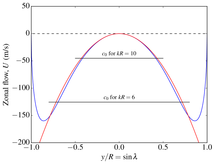
Figure 1: Parabolic zonal flow $U$ (red curve, Eq. 4) in the frame rotating at the equatorial rotation rate, which approximates the Sun’s rotational velocity at the photosphere (blue curve). The horizontal black lines indicate the phase speed of Rossby waves, $c_{0}=-(\beta-U^{\prime\prime})/k^{2}$, for longitudinal wavenumbers $kR=6$ and $kR=10$. There are critical latitudes where $U=c_{0}$.

The two-dimensional Navier-Stokes equations in the equatorial $\beta$ plane are

$$\left(\frac{\partial}{\partial t}+U\frac{\partial}{\partial x}\right)u_{x}+u_{y}U^{\prime}+\boldsymbol{u}\boldsymbol{\cdot}\boldsymbol{\nabla}u_{x}=-\frac{1}{\rho}\frac{\partial p}{\partial x}+\nu\Delta u_{x}+fu_{y},$$ (5)

$$\left(\frac{\partial}{\partial t}+U\frac{\partial}{\partial x}\right)u_{y}+\boldsymbol{u}\boldsymbol{\cdot}\boldsymbol{\nabla}u_{y}=-\frac{1}{\rho}\frac{\partial p}{\partial y}+\nu\Delta u_{y}-fu_{x},$$ (6)

where $\nu$ is the viscosity and the equatorial Coriolis parameter is $f=\beta y$ with $\beta=2\Omega/R$. The prime denotes a derivative, for example $U^{\prime}={\rm d}U/{\rm d}y$.

To enforce mass conservation, we introduce the stream function $\Psi$ such that

$$u_{x}=\frac{\partial\Psi}{\partial y},\qquad u_{y}=-\frac{\partial\Psi}{\partial x}.$$ (7)

Assuming a barotropic fluid, we can eliminate the pressure term by combining the two components of the momentum equation, to obtain

$$\left(\frac{\partial}{\partial t}+U\frac{\partial}{\partial x}\right)\Delta\Psi+\left(\beta-U^{\prime\prime}\right)\frac{\partial\Psi}{\partial x}+(\boldsymbol{u}\boldsymbol{\cdot}\boldsymbol{\nabla})\Delta\Psi=\nu\ \Delta^{2}\Psi.$$ (8)

3 Critical latitudes

3.1 Linear inviscid case: critical points

In the linear inviscid case, we search for wave solutions of the form

$$\Psi(x,y,t)={\rm Re}\left\{\psi(y)\exp[{{\rm i}(kx-\omega t)}]\right\}.$$ (9)

Dropping the nonlinear and viscous terms, Eq. (8) becomes the Rayleigh-Kuo equation (Kuo, 1949):

$$\left(U-c\right)(-k^{2}\psi+\psi^{\prime\prime})+\left(\beta-U^{\prime\prime}\right)\psi=0,$$ (10)

where $c=\omega/k$ is the phase speed. The above equation differs from Rayleigh’s (1879) equation only through the $\beta$ term. It can be rewritten as a Helmholtz equation:

$$\psi^{\prime\prime}+K(y)\psi=0,$$ (11)

with

$$K(y)=-k^{2}+\frac{\beta-U^{\prime\prime}}{U-c}.$$ (12)

The squared latitudinal wavenumber, $K(y)$, is singular at the critical points $y=\pm y_{c}$ such that $U(y_{c})=c$. The critical points divide the low-latitude region where the solution is locally oscillatory ($K>0$ for $|y|<y_{c}$) from the high-latitude regions where it is locally evanescent ($K<0$ for $|y|>y_{c}$).

Equation (10), supplemented by boundary conditions $\psi(\pm R)=0$, is an eigenvalue problem that can be solved in the complex plane. It admits a continuum of neutral modes with real eigenfrequencies. According to Rayleigh’s theorem (adapted for the Rayleigh-Kuo equation, see Kuo, 1949), there is no discrete mode because $\beta-U^{\prime\prime}\neq 0$ everywhere. We can thus solve the initial value problem given by Eq. (10) for any particular real value of $c$ to obtain the associated eigenfunction (e.g., Drazin & Howard, 1966; Drazin et al., 1982; Balmforth & Morrison, 1995). These eigenfunctions are singular at the critical points.

Because $U^{\prime\prime}$ is constant in our problem and $U(0)=0$, Eq. (12) implies that each mode can be associated with a value of $K(0)$ such that

$$c=-\frac{\beta-U^{\prime\prime}}{k^{2}+K(0)}.$$ (13)

For equatorial propagation, $K(0)=0$ is a natural choice, and we may consider the eigenvalue

$$c_{0}=-(\beta-U^{\prime\prime})/k^{2}$$ (14)

as an example. In our case, $\beta-U^{\prime\prime}=1.12\beta$, so waves propagate faster than in the no-flow case. The critical points $y=\pm y_{c}$ where $U(\pm y)=c_{0}$ are given by

$$ky_{c}=\sqrt{\beta R^{2}/\overline{U}+2}=4.31.$$ (15)

Thus, for $kR>4.31$, there are critical latitudes at $\lambda=\pm\lambda_{c}$, such that

$$\lambda_{c}=\arcsin(4.31/kR).$$ (16)

To obtain the eigenfunctions, Eq. (10) should be solved separately for $|y|<y_{c}$ and $|y|>y_{c}$. The analytical and numerical solutions are discussed in Sect. 4. The stream function is continuous ($u_{y}=-{\rm i}k\psi$ is continuous), however its first and second derivatives diverge at the critical layer (see, e.g., Haynes, 2003).

3.2 Viscous critical layer

Bulk viscosity removes singularities. The linear viscous equation for $\psi$ is

$$\left(c-U\right)(-k^{2}\psi+\psi^{\prime\prime})-\left(\beta-U^{\prime\prime}\right)\psi=\frac{{\rm i}\nu}{k}(k^{4}\psi-2k^{2}\psi^{\prime\prime}+\psi^{\prime\prime\prime\prime}).$$ (17)

For $\beta=0$ we recognize the Orr-Sommerfeld equation (Orr, 1907; Sommerfeld, 1909). Equation (17) is a fourth-order differential equation, which requires four boundary conditions, e.g. $\psi(\pm R)=0$ and $\psi^{\prime}(\pm R)=0$ for a no-slip boundary condition. The critical layer of the inviscid case is replaced by a viscous critical layer around $y=\pm y_{c}$. The width of this viscous layer, $\delta$, is obtained by balancing the dominant viscous term with the dominant term on the left-hand side, $(U-c)\psi^{\prime\prime}\sim\nu\psi^{\prime\prime\prime\prime}/k$. Close to the viscous layer, we write ${\rm d}/{\rm d}y\sim 1/\delta$ and $U-c\approx U^{\prime}(y_{c})(y-y_{c})\sim(\overline{U}y_{c}/R^{2})\delta$, so that the width of the viscous layer is approximately

$$\delta/R\sim(ky_{c}\ Re)^{-1/3},$$ (18)

where

$$Re=R\overline{U}/\nu$$ (19)

is the Reynolds number.

The width of the layer is controlled by $Re$. As discussed by Rüdiger (1989), $\nu$ should be understood as an eddy viscosity due to turbulent convection. As an example, we may estimate the Reynolds number associated with solar supergranulation. For supergranulation, the turbulent viscosity $\nu\approx 250$ km²/s (Simon & Weiss, 1997; Duvall, Jr. & Gizon, 2000) implies $Re\approx 700$ and $\delta\approx 0.07R$ for $kR=10$. Not surprisingly, the width of the viscous layer is comparable in this case to the spatial scale of supergranulation.

3.3 Nonlinear critical layer

In order to assess whether it is legitimate to drop the nonlinear term $(\boldsymbol{u}\boldsymbol{\cdot}\boldsymbol{\nabla})\Delta\Psi$ in Eq. (8), we estimate the width of the nonlinear critical layer $\delta_{NL}$. It is obtained by balancing the advection term $k(U-c)\psi^{\prime\prime}$ and the nonlinear term $u_{y}\psi^{\prime\prime\prime}$. We find

$$\delta_{NL}/R\sim\left(u_{\rm max}/\overline{U}\right)^{1/2}(ky_{c})^{-1/2},$$ (20)

where $u_{\rm max}$ is a characteristic velocity amplitude for the Rossby waves. On the Sun, Liang et al. (2019) measured $u_{\rm max}\approx 2$ m/s for the maximum latitudinal velocity of a mode at the equator. For $kR=10$, the width of the nonlinear critical layer is $\delta_{NL}\approx 0.04R$.

Introducing the threshold $Re_{*}=(u_{\rm max}/\overline{U})^{-3/2}(ky_{c})^{1/2}$, the ratio between the widths of the viscous and nonlinear critical layers is

$$\delta/\delta_{NL}\approx(Re/Re_{*})^{-1/3}.$$ (21)

For $Re<Re_{*}$ the critical layer is linear and dominated by dissipation over the width $\delta$. For $kR=10$, we find $Re_{*}\approx 3000$, which is much larger than the Reynolds number $Re\approx 700$ estimated in the previous section for solar supergranulation. Hence, it is not unreasonable to study the linear problem — as we do in the remainder of this paper. However, we caution that there is some uncertainty about the appropriate value for the viscosity.

4 Inviscid modes of oscillation

In the inviscid case, the spectrum for the Rayleigh-Kuo equation, Eq. (10), is real and continuous. We fix the value of $c$ to $c_{0}$ (Eq. 14) and compute the corresponding eigenfunctions. There are two singular solutions, both real: a solution that is symmmetric in latitude and an antisymmetric solution. These solutions can be obtained by solving the equation analytically or numerically in two distinct intervals, $0\leq y<y_{c}$ and $y_{c}\leq y\leq R$.

In the inner region, we solve the ODE with the conditions $\psi(0)=1$ and $\psi^{\prime}(0)=0$ to obtain the symmetric solution. For the region $y>y_{c}$, we impose continuity with the inner solution and use the boundary condition $\psi(R)=0$. The symmetric solution can be expressed as a series in each regions. We write $\psi(y)=\sum_{p\geq 0}a_{p}\xi^{2p}$ with $\xi=y/R$ for $|y|<y_{c}$ and $\psi(y)=\sum_{p\geq 1}b_{p}(\xi^{2}-1)^{p}$ for $|y|>y_{c}$. The coefficients $a_{p}$ and $b_{p}$ are computed by recurrence. Setting $\kappa=kR$ and $\xi_{c}=y_{c}/R$, the inner solution is given by

$$a_{0}=1,$$ (22)

$$a_{1}=0,$$ (23)

$$a_{p}=\frac{2(p-1)(2p-3)a_{p-1}-\kappa^{2}a_{p-2}}{2\xi_{c}^{2}p(2p-1)}\;\textrm{ for }p\geq 2.$$ (24)

For the outer solution,

$$b_{2}= -b_{1}/4,$$ (25)

$$b_{3}= -\frac{[\kappa^{2}+3(1-\xi_{c}^{2})]b_{2}}{6(1-\xi_{c}^{2})},$$ (26)

$$b_{p}= -\frac{[(1-\xi_{c}^{2})(2p-3)+2(p-2)]b_{p-1}}{2(1-\xi_{c}^{2})p}$$

$$+\frac{[\kappa^{2}-2(p-2)(2p-5)]b_{p-2}+\kappa^{2}b_{p-3}}{4(1-\xi_{c}^{2})(p-1)p}\;\textrm{ for }p\geq 4.$$ (27)

The coefficient $b_{1}$ is chosen such that the solution is continuous at the critical point.

To validate the series solution, we also solved the problem numerically. In the inner region, we have an initial value problem that can be solved using classical libraries, for example odeint from SciPy. In the outer region, the problem is a boundary value problem that can be converted into an initial value problem using the shooting method (Keller, 1968).

We find an excellent agreement between the analytical and the numerical solutions, thus we only plot the analytical solution in Fig. 2 for $kR=10$. The symmetric eigenfunction $\psi_{s}$ switches sign before the critical latitude and evanesces above it. The location of the critical layer is close to the zero-crossing of the observed vorticity eigenfunctions from Löptien et al. (2018) and Proxauf et al. (2020). Unfortunately, in the inviscid case, the vorticity $\zeta=k^{2}\psi-\psi^{\prime\prime}$ diverges at the critical latitude and thus the comparison with the observations is difficult.

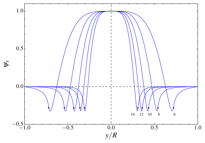
Figure 2: Symmetric inviscid eigenfunctions for the eigenvalue $c_{0}=-(\beta-U^{\prime\prime})/k^{2}$ and $kR=6,8,10,12$ and $14$. The stars mark the critical points.

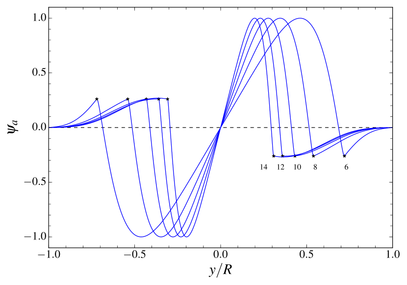
Figure 3: Antisymmetric inviscid eigenfunctions for $c=c_{0}$ and $kR=6,8,10,12$ and $14$. The stars mark the critical points.

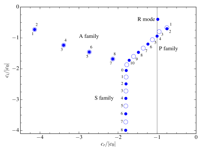
Figure 4: Eigenvalues $c=c_{r}+{\rm i}c_{i}$ in the complex plane for $kR=10$ and $Re=300$, normalized by the reference eigenvalue $|c_{0}|=(\beta-U^{\prime\prime})/k^{2}$. The R mode is clearly identifiable (the least damped mode), as well as the three families of modes: the wall modes (A family), the center modes (P family), and the damped modes (S family). The modes with symmetric eigenfunctions are shown with full circles and the ones with antisymmetric eigenfunctions with open circles. All modes have $c_{r}<0$ and $c_{i}<0$, i.e. they are stable and propagate in the retrograde direction. The vertical line corresponds to the phase speed of the standard Rossby wave, $c_{r}=c_{0}$. Modes in each family are labelled with integers, which increase with attenuation.

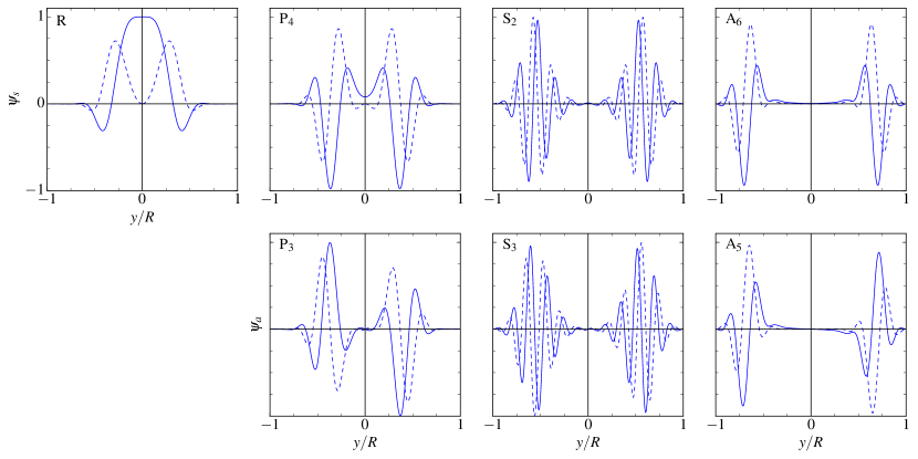
Figure 5: Eigenfunctions for the symmetric modes R, P₄, S₂, and A₆ (top row, $\psi_{s}$) and for the antisymmetric modes P₃, S₃, and A₅ (bottom row, $\psi_{a}$). See Fig. 4 for the position of the corresponding eigenvalues in the complex plane. The real and imaginary parts are plotted with solid and dashed lines respectively. The modulus of the eigenfunctions is normalized to one. By choice, all imaginary parts are zero at the equator.

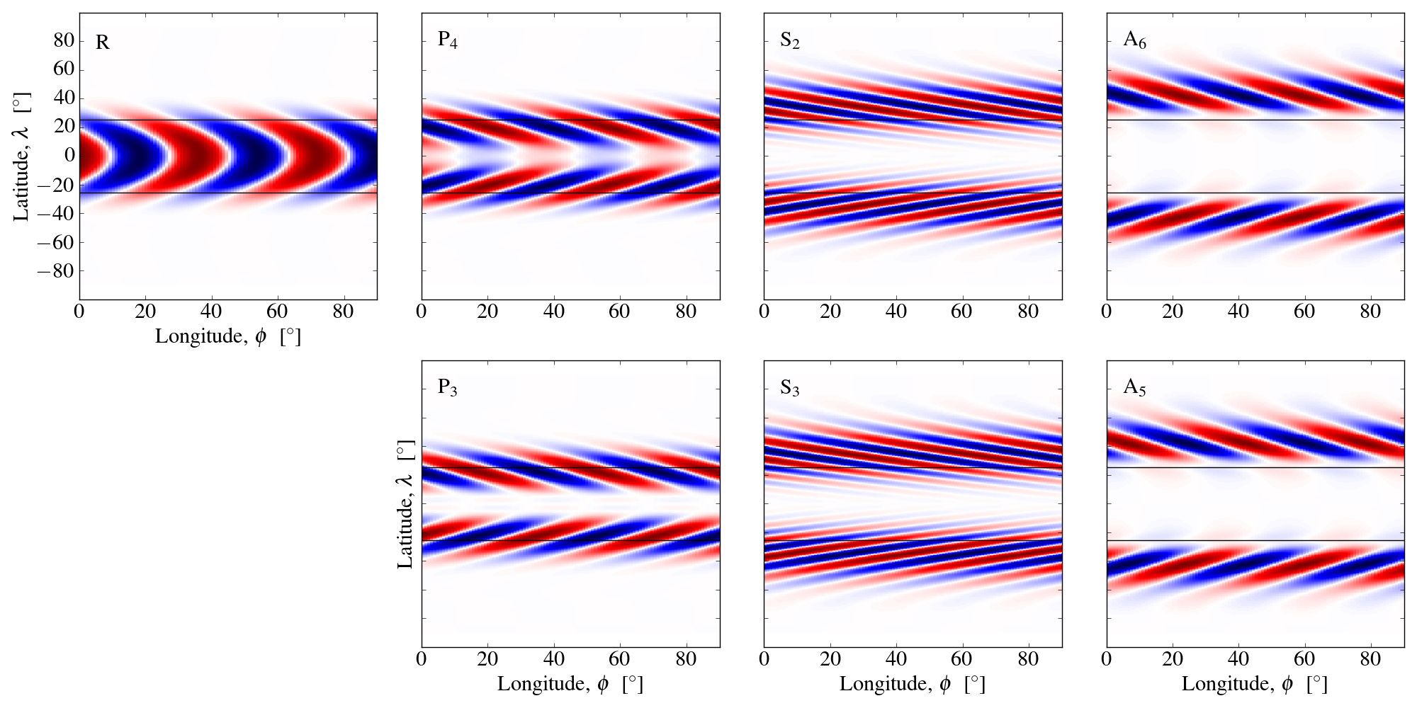
Figure 6: Stream functions in real space for all the modes shown in Fig. 5. Horizontal black lines show the central latitudes of the viscous layers, $\lambda=\pm 25^{\circ}$ for $kR=10$. The R mode (top left panel) is confined to the equatorial region between the viscous layers.

We note that for each eigenvalue $c=c_{0}$ there exists also an antisymmetric eigenfunction, $\psi_{a}$. This solution can be obtained like above, but with different boundary conditions at the equator. We set $\psi_{a}(0)=0$ and $\psi^{\prime}_{a}(0)=\psi^{\prime}_{0}$, where $\psi^{\prime}_{0}$ can be chosen to control the maximum value of $\psi_{a}$, for example unity. The other conditions are the same as before, i.e. $\psi_{a}(\pm R)=0$ and $\psi_{a}$ continuous at the critical point. The antisymmetric solution can be expanded as $\psi_{a}(y)=\sum_{p\geq 0}A_{p}\xi^{2p+1}$ for $|y|<y_{c}$ and $\psi_{a}(y)=\sum_{p\geq 1}B_{p}\xi(\xi^{2}-1)^{p}$ for $|y|>y_{c}$. The coefficients $A_{p}$ an $B_{p}$ are again obtained by recurrence. Figure 3 shows example antisymmetric eigenfunctions.

5 Viscous modes of oscillation

5.1 Numerical method

In order to remove the singularities at the critical latitudes, we now include viscosity. The viscosity is specified through the Reynolds number, $Re$, which is a free parameter in our problem. For example, $Re=700$ for supergranular turbulent viscosity.

To facilitate the numerical resolution of the modified Orr-Sommerfeld equation, Eq. (17), it is convenient to introduce dimensionless quantities. We define $\xi=y/R$, $\kappa=kR$, and $\hat{\beta}=\beta R^{2}/\overline{U}$. The dimensionless eigenvalues $\hat{c}=c/\overline{U}$ and eigenfunctions $\hat{\psi}(\xi)={\psi(y)}/({R\overline{U}})$ solve the equation

$$(\hat{c}+\xi^{2})\hat{D}\hat{\psi}-(\hat{\beta}+2)\hat{\psi}={\rm i}(\kappa\ Re)^{-1}\ \hat{D}^{2}\hat{\psi},$$ (28)

where $\hat{D}=-\kappa^{2}+{\rm d}^{2}/{\rm d}\xi^{2}$ is the Laplacian and the prime now denotes derivation with respect to $\xi$. For $\overline{U}=244$ m/s, we have $\hat{\beta}=16.4$. We consider values of the dimensionless longitudinal wavenumber in the range $8\leq\kappa\leq 15$.

We follow the numerical approach of Orszag (1971), originally developed for the Orr-Sommerfeld eigenvalue problem. We use the Matlab package Chebfun to project functions onto Chebyshev polynomials and to compute spatial derivatives analytically (Driscoll et al., 2014). This package also provides practical tools to solve differential equations and eigenvalue problems (only a few lines of codes are needed).

To obtain the symmetric solutions, we solve the above eigenvalue problem on $[0,1]$ with the boundary conditions

$$\hat{\psi}^{\prime}_{s}(0)=\hat{\psi}_{s}^{\prime\prime\prime}(0)=0\quad\text{and}\quad\hat{\psi}_{s}(1)=\hat{\psi}^{\prime}_{s}(1)=0.$$ (29)

The antisymmetric solutions are obtained by setting

$$\hat{\psi}_{a}(0)=\hat{\psi}_{a}^{\prime\prime}(0)=0\quad\text{and}\quad\hat{\psi}_{a}(1)=\hat{\psi}^{\prime}_{a}(1)=0.$$ (30)

In both cases, the numerical solutions (eigenvalues and eigenfunctions) are complex.

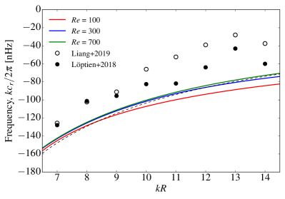
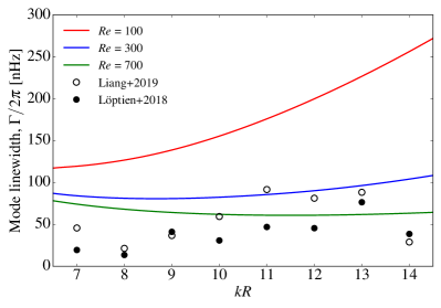
Figure 7: Left panel: R-mode dispersion relations $\omega=kc_{r}$ for $Re=100$, 300 and 700 (red, blue and green). The dashed black curve is the reference dispersion relation $\omega=kc_{0}$. For comparison, the frequencies of each mode $m$ observed by Löptien et al. (2018) and Liang et al. (2019) are multiplied by the factor $(m+1)/kR$ and plotted at abscissa $kR$ (this simple conversion factor is derived from the dispersion relations for classical Rossby waves in spherical and local Cartesian geometries). Right panel: Plot of $\Gamma=-2kc_{i}$ for $Re=100$, 300 and 700. The observed full widths at half maximum for each mode $m$ are plotted at abscissa $kR$ for comparison.

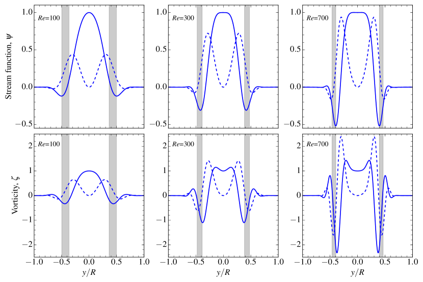
Figure 8: Stream function (top row) and vertical vorticity (bottom row) for R modes with $kR=10$. The Reynolds number is $Re=100$, 300 and 700 from left to right. The solid and dashed curves correspond to the real and imaginary parts. The shaded areas indicate the locations of the viscous critical layers for each value of $Re$.

5.2 Spectrum

In Fig. 4 the eigenvalues $c=c_{r}+{\rm i}c_{i}$ are shown in the complex plane for $\kappa=10$ and $Re=300$. In the figure, these eigenvalues are normalized by $|c_{0}|>0$. All modes are stable since none of the imaginary parts of the eigenfrequencies are positive. In the complex plane, the eigenvalues are distributed along three main branches that correspond to different types of eigenfunctions. The same branches appear in the standard plane Poiseuille problem; they have been called A, P and S by Mack (1976). Example eigenfunctions are displayed in Fig. 5 and Fig. 6. The A branch, for which the eigenfunctions have large amplitudes at high latitudes, refers to the “wall modes”. The P branch refers to the “center modes” which oscillate near the viscous layers. The S branch corresponds to the “damped modes” (Schensted, 1961). Schensted (1961) showed that the A and P branches have a finite number of eigenvalues and the S branch has an infinite number of eigenvalues. She obtained approximate equations for the three branches. We labelled the modes with integers in Fig. 4, such that even integers refer to the symmetric eigenfunctions and odd integers to the antisymmetric eigenfunctions. As noted by Drazin & Reid (2004), the even and odd modes in the A branch have nearly the same eigenfrequencies. As seen in Fig. 6, the A modes have significant amplitudes only at latitudes above the viscous layers.

Our problem differs from the standard plane Poiseuille problem through the $\beta$ term. As a result, one additional mode appears in the eigenvalue spectrum (Fig. 4). This mode, which we call the R mode for an obvious reason, is symmetric and has an eigenfrequency whose real part is close to that of the classical equatorial Rossby mode, $c_{r}\approx c_{0}$. The R mode is the mode with the longest lifetime in the spectrum. It is also the mode for which $\int_{-1}^{1}|\hat{\psi}^{\prime\prime}|^{2}{\rm d}\xi$ is the smallest. As seen in Fig. 5, the real part of the R-mode eigenfunction resembles the eigenfunction of the symmetric mode found in the inviscid case (Fig. 2), except that it is smooth everywhere (no infinite derivative at the critical points). In the viscous case, the complex R-mode eigenfunctions look like chevrons in real space (Fig. 6).

Notice that there are modes in the P branch with $c_{r}$ close to $c_{0}$ (P₃ and P₄), however these modes have a much shorter lifetime than the R mode (by a factor of two to three at $Re=300$) and eigenfunctions that differ significantly from the observations.

5.3 R modes

Figure 7 shows the R-mode eigenfrequencies as a function of wavenumber $kR$ for different values of the viscosity. The value of the viscosity has a rather small effect on the dispersion relation. At fixed wavenumber, the real part of the eigenfrequency changes with $Re$ by less than ten percent over the range $100\geq Re\geq 700$. On the other hand, the imaginary part $c_{i}$ changes significantly with the value of $Re$. For $Re<700$, the attenuation $\Gamma=-2kc_{i}$ increases with $k$. For $Re=300$, we find that the theoretical mode linewidths ($\Gamma/2\pi=-kc_{i}/\pi$ in nHz) are in the range $70$ – $100$ nHz, i.e. in reasonable agreement with the observed mode linewidths ($\Gamma/2\pi$ from Liang et al., 2019). Note that a mode’s $e$-folding lifetime is given by $\tau=2/\Gamma$.

The top row of Fig. 8 shows the R-mode stream functions for different values of the Reynolds number. The normalization is such that, at $\xi=0$, the real part is one and the imaginary part is zero. As $Re$ decreases, the stream function varies more slowly around the viscous layer and its imaginary part gets smaller in amplitude. The bottom row of Fig. 8 shows the vertical vorticity eigenfunctions. Notice the fast variations near the viscous layer for $Re=700$, where $\psi^{\prime\prime}$ is largest.

6 Influence of the meridional flow

In addition to the rotational shear $U$, here we include the effect of the meridional flow $V$ on the R mode. The total velocity is

$$U(y)\boldsymbol{\hat{x}}+V(y)\boldsymbol{\hat{y}}+\boldsymbol{u}(x,y,t),$$ (31)

where the meridional flow is approximated by

$$V(y)=\overline{V}\ \frac{y}{R}\left[1-\left(\frac{y}{R}\right)^{2}\right],$$ (32)

with

$$\overline{V}=\frac{3\sqrt{3}}{2}\times 15\ \text{m/s}.$$ (33)

The value of $\overline{V}$ is chosen such that the maximum value of $V$ is 15 m/s (near latitude $\lambda=35^{\circ}$).

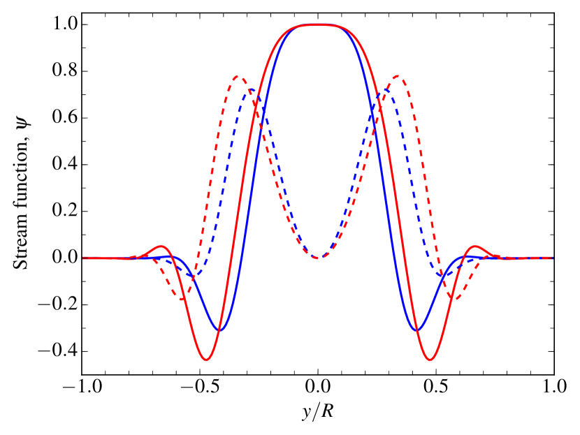
Figure 9: Effect of the meridional flow $V$ on the R-mode stream function for $Re=300$ and $kR=10$ (red curves). For comparison, the blue curves show the stream function when only the zonal flow $U$ is included. The real and imaginary parts correspond to the solid and dashed curves.

Including the meridional flow, the two-dimensional linearized Navier-Stokes equations in the equatorial $\beta$ plane become

$$\left(\frac{\partial}{\partial t}+U\frac{\partial}{\partial x}+V\frac{\partial}{\partial y}\right)u_{x}+u_{y}U^{\prime}=-\frac{1}{\rho}\frac{\partial p}{\partial x}+\nu\Delta u_{x}+fu_{y},$$ (34)

$$\left(\frac{\partial}{\partial t}+U\frac{\partial}{\partial x}+V\frac{\partial}{\partial y}\right)u_{y}+u_{y}V^{\prime}=-\frac{1}{\rho}\frac{\partial p}{\partial y}+\nu\Delta u_{y}-fu_{x}.$$ (35)

Combining these equations, the fourth-order differential equation for the stream function (linear problem) is

$$\left(c-U+\frac{{\rm i}V^{\prime}}{k}\right)D\psi+\frac{{\rm i}V}{k}D\psi^{\prime}-\left(\beta-U^{\prime\prime}\right)\psi=\frac{{\rm i}\nu}{k}D^{2}\psi,$$ (36)

with $D=-k^{2}+{\rm d}^{2}/{\rm d}y^{2}$. Compared to the previous problem with $U$ only, the term in front of $D\psi$ is now complex and an additional term involving the first and third derivatives of the stream function appear.

We consider only the symmetric solutions and focus on the R mode. The boundary conditions are $\psi^{\prime}(0)=\psi^{\prime\prime\prime}(0)=0$ and $\psi(R)=\psi^{\prime}(R)=0$. Like before, we follow the procedure by Orszag (1971) to solve the eigenvalue problem. The eigenfrequencies are not affected significantly by the meridional flow. For $Re=300$ and $kR=10$, we find $c/|c_{0}|=-0.986-0.446{\rm i}$ when $U$ and $V$ are included, compared to $c/|c_{0}|=-0.982-0.398{\rm i}$ when only $U$ is included. Figure 9 shows the real and imaginary parts of the R-mode eigenfunction at fixed $kR=10$ for $Re=300$. The meridional flow $V$ has a small but measurable influence on the $\psi$ eigenfunction: it is stretched towards higher latitudes and its real part has a larger amplitude near the viscous layers.

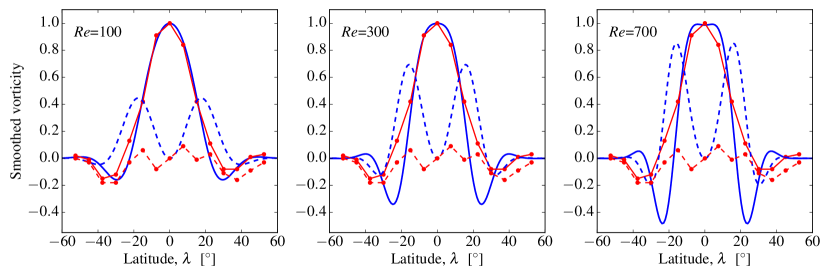
Figure 10: Real (blue solid lines) and imaginary (blue dashed lines) parts of the R-mode vertical vorticity at $kR=10$ after smoothing the maps of horizontal velocities with a 2D Gaussian kernel with $\sigma=6^{\circ}$. Three different values of $Re$ are shown. For comparison, the red curves with points show the ring-diagram helioseismic observations for $m=10$ near the surface (Proxauf et al., 2020).

7 Comparison with observations

Proxauf et al. (2020) measured and characterized the vorticity eigenfunctions of the solar Rossby modes using ring-diagram helioseismic analysis. To enable a direct comparison between observations and theory, some smoothing must be applied to the model because the observed flows have a resolution of only $\sigma=6^{\circ}$ in $\phi$ and $\lambda$. After remapping the theoretical flows on a longitude-latitude grid, we convolve $u_{\phi}$ and $u_{\lambda}$ with a 2D Gaussian kernel with standard deviation $\sigma$ in both coordinates. From the smoothed velocities, we compute the vertical vorticity. As seen in Fig. 10, the smoothing has a significant effect on the theoretical vorticity near the viscous layer.

The functional form of the real part of the observed eigenfunction was described by several parameters by Proxauf et al. (2020): a full width at half maximum $W$, the latitude $\lambda_{0}$ where the sign changes, the latitude $\lambda_{\rm min}$ where the vorticity is most negative, and the value $\zeta_{\rm min}$ of the vorticity at $\lambda_{\rm min}$. These parameters are provided in Table 1 for three different values of $kR$ in three different cases: (a) smoothed theoretical vorticity when the zonal shear flow $U$ is included, (b) smoothed theoretical vorticity when $U$ and $V$ are both included and (c) observations from Proxauf et al. (2020). For $Re=300$, we find that the widths for cases (a) and (b) are within $\approx 3^{\circ}$ of the observed values. For (a), the zero-crossing latitude varies from $\lambda_{0}=17^{\circ}$ for $kR=12$ to $\lambda_{0}=21^{\circ}$ for $kR=8$. For (b) the values of $\lambda_{0}$ are slightly higher by $\approx 2^{\circ}$, while the observed $\lambda_{0}\approx 28^{\circ}$ does not vary much with $k$. The theoretical values of $\lambda_{\min}$ vary with $kR$ a little faster than $\lambda_{0}$, and theory is in better agreement with observations for $kR=8$. The observed values of $\zeta_{\rm min}$ range from $-0.3$ to $-0.1$, about half of the theoretical values. However, the values of $\zeta_{\rm min}$ depend on $Re$, with more negative values for larger values of $Re$. On the other hand, the values of $W$, $\lambda_{0}$, and $\lambda_{\rm min}$ in the table are not very sensitive to the Reynolds number for $100\leq Re\leq 700$.

The imaginary part of the vorticity eigenfunctions is a lot more difficult to measure (Proxauf et al., 2020). It is significantly different from zero for some values of $m$, however it is noisy and its functional form cannot be described by a simple parametric function. According to Proxauf et al. (2020), the sign of the observed imaginary part appears to be positive for the smallest values of $m$ and negative for $m>5$. The comparison provided in Fig. 10 shows that, at latitudes below the viscous layer, the amplitude of the imaginary part is much higher in the model than in the observations.

Table 1: Parameters $W$, $\lambda_{0}$, $\lambda_{\rm min}$ and $\zeta_{\rm min}$ characterizing the functional form of the real part of the R-mode vorticity eigenfunctions. The smoothed eigenfunctions from theory ($Re=300$) are given for the cases when (a) only the zonal flow $U$ is included and (b) both $U$ and the meridional flow $V$ are included. The theoretical values are compared with the observations from Proxauf et al. (2020).

	Case	$kR=8$	$kR=10$	$kR=12$
$W$ $(^{\circ})$	$U$	$17.6$	$13.1$	$11.2$
	$U$ & $V$	$20.2$	$15.8$	$13.1$
	Obs.	$17.1\pm 0.8$	$14.7\pm 1.1$	$13.8\pm 1.4$
$\lambda_{0}$ $(^{\circ})$	$U$	$21.1$	$18.4$	$17.5$
	$U$ & $V$	$24.8$	$20.2$	$19.4$
	Obs.	$25.8$	$27.8\pm 1.6$	$28.9\pm 1.0$
$\lambda_{\rm min}$ $(^{\circ})$	$U$	$29.3$	$24.8$	$22.9$
	$U$ & $V$	$32.9$	$27.4$	$24.8$
	Obs.	$36.5\pm 1.8$	$34.5\pm 2.1$	$39.8\pm 1.8$
$\zeta_{\rm min}$	$U$	$-0.69$	$-0.35$	$-0.17$
	$U$ & $V$	$-0.86$	$-0.49$	$-0.28$
	Obs.	$-0.28$	$-0.11$	$-0.14$

8 R-mode momentum fluxes

The complex eigenfunctions in our model imply that R modes transport a net momentum flux in latitude. It is interesting to obtain an estimate of this momentum flux (even though the model eigenfunctions have imaginary parts that differ from the observations). The purpose of this exercise is to establish whether R modes play a significant role in the balance of forces that shape differential rotation.

Let us consider a time-dependent zonal flow $U(y,t)$, which evolves slowly according to the $x$-component of the momentum equation averaged over $x$ (see, e.g., Geisler & Dickinson, 1974):

$$\frac{\partial U}{\partial t}=-\frac{\partial}{\partial_{y}}\langle u_{x}u_{y}\rangle+\nu U^{\prime\prime}+V(\beta y-U^{\prime}),$$ (37)

where the prime denotes a $y$-derivative and angle brackets $\langle\cdot\rangle$ denote the average over $x$. We used $\partial_{x}u_{x}+\partial_{y}u_{y}=0$ to obtain the term involving $\langle u_{x}u_{y}\rangle$ on the right-hand side of the equation. The various terms in Eq. (37) have been discussed in detail by Rüdiger (1989) in spherical geometry. These terms must balance exactly to explain the steady-state differential rotation.

In our problem the horizontal Reynolds stress has two components, the first one due to rotating turbulent convection (the $\Lambda$ effect) and the other one due to the Rossby waves,

$$\langle u_{x}u_{y}\rangle=\langle u_{x}u_{y}\rangle_{\rm R}+\langle u_{x}u_{y}\rangle_{\Lambda}.$$ (38)

Let us estimate $\langle u_{x}u_{y}\rangle_{\rm R}$ in the model for a single R mode. It is related to the stream function through

$$\langle u_{x}u_{y}\rangle_{\rm R} {\color[rgb]{0,0,0}=-\left\langle\frac{\partial\Psi}{\partial y}\ \frac{\partial\Psi}{\partial x}\right\rangle}$$

$${\color[rgb]{0,0,0}=-\left\langle{\rm Re}\left(\psi^{\prime}e^{{\rm i}k(x-c_{r}t)-t/\tau}\right)\ {\rm Re}\left({\rm i}k\psi e^{{\rm i}k(x-c_{r}t)-t/\tau}\right)\right\rangle}$$

$$=-\frac{k}{2}\text{ Im}\left(\psi^{\prime}\psi^{*}\right)e^{-2t/\tau}=:Q_{xy}\ e^{-2t/\tau},$$ (39)

where $\tau$ is the mode lifetime mentioned in Sect. 5.3. We normalize the R-mode stream function such that the velocity amplitude at the equator is equal to its observed value,

$$k\psi(0)=u_{\rm max}\approx 2\textrm{ m/s}.$$ (40)

The Reynolds stress $Q_{xy}$ is plotted in Fig. 11 for R modes with $Re=300$ and $kR=8$, 10 and 12. We find that $Q_{xy}<0$ in the north, below the viscous critical layer. For example, for $kR=10$, $Q_{xy}$ reaches the minimum value of $-2$ m²/s² at latitude $20^{\circ}$. This means that R modes transport angular momentum from the dissipation layer to the equator, i.e. reinforce latitudinal differential rotation. This is the expected result for idealized Rossby waves incident on a critical layer (see, e.g., Vallis, 2006).

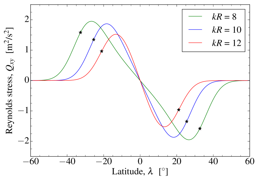
Figure 11: Horizontal Reynolds stress $Q_{xy}$ versus latitude for R modes with $kR=8$, 10 and 12. The Reynolds number is $Re=300$ and mode amplitudes were normalized according to Eq. (40). Both the zonal flow $U$ and the meridional flow $V$ were included to compute the mode eigenfunctions. The stars show the locations of the viscous critical layer for the different values of $kR$.

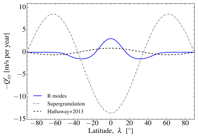
Figure 12: Equatorial acceleration $-\partial_{y}Q_{xy}$ due to the superposition of nine viscous R modes for $kR=7,8,\dots 15$ (blue solid curve). The dot-dashed and dashed curves show $-\partial_{y}\langle u_{x}u_{y}\rangle$ for supergranulation (Hanasoge et al., 2016, their figure 10) and larger-scale convection (Hathaway et al., 2013) respectively. For reference, the solar “torsional oscillation” has a typical amplitude of about $\pm 5$ m/s (see, e.g., Lekshmi et al., 2018).

Summing $Q_{xy}$ over several R modes would lead to a horizontal Reynolds stress that is comparable in amplitude and sign to the value reported at large spatial scales by Hathaway et al. (2013). On the other hand, $Q_{xy}$ has the opposite sign and is much smaller in amplitude than the (viscous) Reynolds stress associated with convective flows at supergranulation scales (Hanasoge et al., 2016, their figure 10). The acceleration $-\partial_{y}Q_{xy}$ is plotted in Fig. 12 and compared to the above mentioned measurements. We see that Rossby waves in our model contribute to the equatorial acceleration at a significant level.

9 Conclusion

Using a simple two-dimensional setup in the $\beta$ plane, we have shown that latitudinal differential rotation and viscosity must play an important role in shaping the horizontal eigenfunctions of global-scale Rossby modes. Viscous critical layers form around latitudes where $c=U$. We find that only one symmetric mode, which we called the R mode, has an eigenvalue whose real part is close to that of the classical sectoral Rossby mode and whose imaginary part is close to the observed value when $Re\approx 300$. The real part of the vorticity eigenfunctions can be made to agree qualitatively with solar observations (unlike the imaginary part).

Treating this problem as a stability problem for a viscous Poiseuille flow in the $\beta$ plane enabled us to connect to prior results in the fluids literature. For example, we used a well-established method to solve the Orr-Sommerfeld equation numerically and we easily identified the known families of modes A, P and S in the complex plane (eigenvalues and eigenfunctions). A new aspect of our work is the identification of the viscous R mode, due to the $\beta$ term in the equation. We find that the combination of the shear flow and the viscosity lead to chevron-shaped eigenfunctions, and thus to non-zero angular momentum transport by R modes. In our model, horizontal Reynolds stresses due to R modes lead to significant equatorial acceleration. Another original aspect of our work is the study of the influence of the solar meridional flow on R modes. We found that the meridional flow affects the eigenfunctions to measurable levels. Reynolds stresses have significantly larger amplitudes when the meridional flow is included, although the meridional flow plays a much smaller role than the differential rotation in shaping the eigenfunctions.

Sophisticated 3D models (but without background shear flow) also include Rossby waves as a possible mechanism to produce equatorial super-rotation in the atmospheres of planets (e.g., Liu & Schneider, 2011; Read & Lebonnois, 2018) and exoplanets (e.g., Showman & Polvani, 2011). Clearly, the present work will have to be extended to three dimensions (see, e.g., Watts et al., 2004, for the eigenvalues in the inviscid case) to account for the radial gradients of solar rotation measured by helioseismology. Also, a better understanding of Rossby waves will benefit from more realistic numerical experiments (see Bekki et al., 2019). Finally, we note that the model developed here can be used to estimate the temporal changes in the Rossby wave frequencies due to the solar-cycle variations in the zonal flows (Goddard et al., 2020).