Quantum Many-Body Simulations of the 2D Fermi-Hubbard Model in Ultracold Optical Lattices

Abstract

Understanding quantum many-body states of correlated electrons is one main theme in modern condensed matter physics. Given that the Fermi-Hubbard model, the prototype of correlated electrons, has been recently realized in ultracold optical lattices, it is highly desirable to have controlled numerical methodology to provide precise finite-temperature results upon doping, to directly compare with experiments. Here, we demonstrate the exponential tensor renormalization group (XTRG) algorithm [Phys. Rev. X 8, 031082 (2018)], complemented with independent determinant quantum Monte Carlo (DQMC) offer a powerful combination of tools for this purpose. XTRG provides full and accurate access to the density matrix and thus various spin and charge correlations, down to unprecedented low temperature of few percents of the fermion tunneling energy scale. We observe excellent agreement with ultracold fermion measurements at both half-filling and finite-doping, including the sign-reversal behavior in spin correlations due to formation of magnetic polarons, and the attractive hole-doublon and repulsive hole-hole pairs that are responsible for the peculiar bunching and antibunching behavior of the antimoments.

Introduction.— The Fermi-Hubbard model, describing a paradigmatic quantum many-body system Hubbard and Flowers (1963); Gutzwiller (1963), has relevance for a broad scope of correlation phenomena, ranging from high-temperature superconductivity Lee et al. (2006), metal-insulator transition Fazekas (1999), quantum criticality Sachdev (2011), to interacting topological states of matter Wen (2004).Yet, puzzles remain in this strongly interacting many-body model after several decades of intensive investigations. In solid-state materials, the Fermi-Hubbard model is often complicated by multi-band structures and interactions such as spin-orbital and Hund’s couplings Georges et al. (2013), etc. In this regard, recent progresses in two-dimensional (2D) fermionic optical lattices, where the interplay between the spin and charge degrees of freedom in the Fermi-Hubbard model has been implemented in a faithful way Bakr et al. (2009); Parsons et al. (2015); Greif et al. (2016); Boll et al. (2016); Cheuk et al. (2016a, b); Parsons et al. (2016), enables a very clean and powerful platform for simulating its magnetic Greif et al. (2013); Hart et al. (2015); Mazurenko et al. (2017); Brown et al. (2017); Hilker et al. (2017); Chiu et al. (2019); Salomon et al. (2019); Koepsell et al. (2019) and transport properties Nichols et al. (2019); Brown et al. (2019).

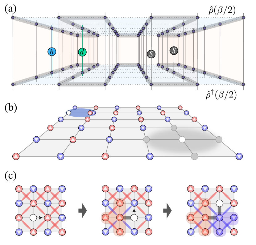
Figure 1: (a) Bilayer calculation of the spin-spin $\langle\hat{S}_{i}\cdot\hat{S}_{j}\rangle$ and hole-doublon $\langle\hat{h}_{i}\cdot\hat{d}_{j}\rangle$ correlators by sandwiching corresponding operators in between $\hat{\rho}(\beta/2)$ and $\hat{\rho}^{\dagger}(\beta/2)$ where the snake-like ordering of sites for the XTRG is indicated by thick gray line. (b) In the low-temperature AF background (blue down and red up spins), a magnetic polaron (grey shaded region) emerges around a moving hole, where the spins around the hole can be in a superposition of spin-up and down states. The blue ellipse represents a hole-doublon pair showing a strong bunching effect. (c) A hole moves in the system along the path indicated by the grey string, leading to a sign reversal of the diagonal spin correlation. The red- and blue-shaded regions illustrate the deformed magnetic background due to the interplay between the hole and spins. Diagonal correlations are indicated red (aligned) or blue (antialigned).

With the state-of-the-art quantum gas microscope techniques, single-site and spin-resolved imaging is now available, and “snapshots” of correlated fermions have been studied experimentally Bakr et al. (2009); Parsons et al. (2015); Greif et al. (2016); Cheuk et al. (2016a). On top of that, detailed local spin and charge correlations Greif et al. (2013); Parsons et al. (2016); Cheuk et al. (2016b); Boll et al. (2016); Mazurenko et al. (2017); Koepsell et al. (2019), as well as hidden orders revealed by pattern recognition Hilker et al. (2017); Chiu et al. (2019), all inaccessible in traditional solid-state experiments, can be read out by the microscope. As a highly controlled quantum simulator, ultracold fermions in optical lattices therefore serve as a promising tool for resolving various intriguing theoretical proposals on the 2D Fermi-Hubbard model. However, numerous challenges remain, both theoretically and experimentally. The currently lowest achievable temperature is f $T/t\simeq 0.25$-0.5 (with $t$ the fermion tunneling energy) on a finite-size system with about 70-80 ⁶Li atoms Mazurenko et al. (2017); Chiu et al. (2019); Koepsell et al. (2019), and $T/t\sim 1$ in ⁴⁰K systems Cheuk et al. (2016a); Hartke et al. (2020). These temperatures are still much higher than the estimated superconductivity transition temperature, $T_{c}/t\sim 0.05$, near the optimal doping of the square-lattice Hubbard model Lee et al. (2006); Chen et al. (2013).

On the theoretical side, it is then of vital importance to provide precise quantum many-body calculations in the 2D Hubbard model for systems of similar size and fermion number as those studied experimentally. Only with that, can one benchmark theory with the cold-atom experiment, determine the effective temperature $T$ of the fermionic optical lattice system, explain experimental results, and provide accurate guidance for future progress. However, accurately computing properties of 2D Fermi-Hubbard model at finite temperature and finite doping is difficult. Quantum Monte Carlo (QMC) methods suffer from the minus-sign problem, although with finite size and temperature, the QMC simulation can actually be performed, yielding unbiased results before one hits the “exponential wall”. In this regard, it is highly desirable to have an alternative and powerful method whose accessible parameter space overlaps, on the one hand, with that of QMC for benchmarking purposes, but which extends, on the other hand, to more difficult yet experimentally accessible regions. In this letter, we demonstrate that the thermal tensor network approach stands out as the method of choice.

In fact, various tensor renormalization group (TRG) methods have been developed to compute the $T=0$ properties of the 2D Hubbard model Noack et al. (1994); Corboz et al. (2010); Kraus et al. (2010); Gu et al. (2010); LeBlanc et al. (2015); Zheng et al. (2017); Qin et al. (2019); Chung et al. (2020). However, the $T>0$ properties at finite doping are much less explored. In this work, we generalize the exponential TRG (XTRG) from spin system Chen et al. (2018); Li et al. (2019) to strongly interacting fermions, and employ it to simulate the Fermi-Hubbard model at both half-filling and finite doping, down to a few percents of the tunneling energy $t$. We compare the results obtained from both XTRG and determinant QMC (DQMC) Han et al. (2019) in the parameter space where both methods are applicable, and find excellent agreement between them as a consistency and sanity check. Then we carry out XTRG$+$DQMC investigations of the 2D Hubbard model to cover the entire parameter space accessed by current cold-atom experiments. We find that the experimental quantum gas microscope data can be perfectly explained by our numerical simulations. The combined scheme of XTRG$+$DQMC therefore opens a route for systematic investigation of the finite-temperature phase diagram of the 2D Fermi-Hubbard model and constitutes an indispensable theoretical guide for ultracold fermion experiments.

The Fermi-Hubbard model.— We consider interacting electrons on a 2D square lattice described by the Hamiltonian

$$H=-t\sum_{\langle{i},\hskip 0.70004pt{j}\rangle,\sigma}(\hat{c}_{{i},\sigma}^{\dagger}\hat{c}_{{j},\sigma}^{\phantom{\dagger}}+{h.c.})+U\sum_{i}\hat{n}_{i\uparrow}\hat{n}_{i\downarrow}-\mu\sum_{{i},\sigma}{\hat{n}_{{i},\sigma}},$$ (1)

with $t=1$ the nearest-neighbor hopping amplitude (which thus sets the unit of energy, throughout), $U>0$ the on-site Coulomb repulsion, and $\mu$ the chemical potential controlling the electron filling. The fermionic operator $\hat{c}_{{i},\sigma}$ annihilates an electron with spin $\sigma\in\{\uparrow,\downarrow\}$ on site ${i}$, and $\hat{n}_{{i},\sigma}\equiv\hat{c}_{{i},\sigma}^{\dagger}\hat{c}_{{i},\sigma}^{\phantom{\dagger}}$ is the local number operator.

In the large-$U$ limit $(U\gg t)$ and at half-filling ($\mu=U/2$), the Hubbard model can be effectively mapped to the Heisenberg model with interchange integral $J=4t^{2}/U$, giving rise to a Néel-ordered ground state with strong antiferromagnetic (AF) correlations at low temperature [depicted schematically in Fig. 1(b)]. This has been demonstrated in many-body calculations Varney et al. (2009) and recently observed in ultracold fermion experiments Mazurenko et al. (2017). In this work, we study the Fermi-Hubbard model with $U=7.2$, a typical interaction strength used in recent experiments  Cheuk et al. (2016a); Mazurenko et al. (2017); Chiu et al. (2019); Hartke et al. (2020), and further tune the chemical potential $\mu<U/2$ to investigate the effect of hole doping.

Fermion XTRG.— Finite-temperature TRG methods have been proposed to compute the thermodynamics of interacting spins Verstraete et al. (2004); Zwolak and Vidal (2004); Feiguin and White (2005); Li et al. (2011); Chen et al. (2017, 2018); Bruognolo et al. (2017); Chung and Schollwöck (2019). However, the simulation of correlated fermions at finite temperature has so far been either limited to relatively high temperature Khatami and Rigol (2011); Czarnik and Dziarmaga (2014) or to rather restricted geometries, like 1D chains Dong et al. (2017). XTRG employs a DMRG-like setup for both 1D and 2D systems Chen et al. (2018); Li et al. (2019) and cools down the systems exponentially fast in temperature. It has been shown to have great precision in simulating quantum spin systems on bipartite Chen et al. (2018) and frustrated lattices Chen et al. (2019); Li et al. (2020). It thus holds great promise to be generalized to correlated fermions.

As shown in Fig. 1(a), we represent the density matrix $\hat{\rho}(\beta/2)$ as a matrix product operator (MPO) defined on a 1D snake-like path [depicted as grey shaded lines in Fig. 1(a)]. To accurately compute the expectation value of a observable $\hat{O}$, we adopt the bilayer technique Dong et al. (2017), yielding $\langle\hat{O}\rangle=\frac{1}{\mathcal{Z}}\mathrm{Tr}[\hat{\rho}(\beta/2)\cdot\hat{O}\cdot\hat{\rho}^{\dagger}(\beta/2)],$ with $\mathcal{Z}=\mathrm{Tr}[\hat{\rho}(\beta/2)\cdot\hat{\rho}^{\dagger}(\beta/2)]$ the partition function. In practice, we adopt the QSpace framework Weichselbaum (2012, 2020) and implement fermion and non-abelian symmetries in our XTRG code (for technical details, see SM ). We consider mainly two-site static correlators, $\langle\hat{O}\rangle=\langle\hat{O}_{i}\cdot\hat{O}_{j}\rangle$, with $\hat{O}_{i}$ a local operator such as the SU(2) spinor $\hat{S}_{i}\equiv[\frac{-1}{\sqrt{2}}\hat{c}_{i\uparrow}^{\dagger}\hat{c}_{i\downarrow}^{\phantom{\dagger}},\frac{1}{2}(\hat{n}_{i\uparrow}-\hat{n}_{i\downarrow}),\frac{1}{\sqrt{2}}\hat{c}_{i\downarrow}^{\dagger}\hat{c}_{i\uparrow}^{\phantom{\dagger}}]^{T}$, the fermion number $\hat{n}_{i}\equiv\hat{n}_{i\uparrow}+\hat{n}_{i\downarrow}$, the occupation projectors $\hat{h}_{i}\equiv|0\rangle\langle 0|_{i}$ (hole) and $\hat{d}_{i}\equiv\left|\uparrow\downarrow\rangle\langle\uparrow\downarrow\right|_{i}\equiv\hat{n}_{i\uparrow}\hat{n}_{i\downarrow}$ (doublon), etc. The spin-spin $\langle\hat{S}_{i}\cdot\hat{S}_{j}\rangle$ and hole-doublon $\langle\hat{h}_{i}\cdot\hat{d}_{j}\rangle$ correlations are schematically depicted in Fig. 1(a).

In our XTRG simulations, we consider the $L\times L$ square-lattice Hubbard model with $L=4,6,8$ with open boundary conditions, facilitating direct comparisons to optical-lattice measurements. We also fully implement non-Abelian spin and particle-hole (i.e., charge) symmetries. This allows us to reduce the $D$ states retained in XTRG to an effective dimension of $D^{\ast}$ multiplets. To be specific, for the half-filled case we exploit SU(2)${}_{\rm charge}\,\otimes$ SU(2)_spin, and for the doped case U(1)${}_{\rm{charge}}\,\otimes$SU(2)_spin symmetry. In practice, this yields an effective dimensional reduction of $D/D^{\ast}\sim 5.6$ and 2.6, respectively. This corresponds to a $(D/D^{\ast})^{4}\simeq 30$-$1000$ fold reduction of computation time in the finite-$T$ simulations, guaranteeing high efficiency and accuracy for fermion simulations. We obtain very well converged XTRG results on the $L=8$ square lattice at half filling (total site number $N=L^{2}=64$) using up to $D^{\ast}=900$ multiplets ($D\simeq 5,000$ states), and on the $L=6$ lattice upon doping using up to $D^{\ast}=1,200$ multiplets ($D\simeq 3,100$ states) SM down to temperatures $T/t\simeq 0.06$ which is unprecedentedly low for such system sizes.

The DQMC simulation performed here is of the finite temperature version with fast update Assaad and Evertz (2008), which has been successfully exploited in the finite-temperature simulation of 2D Hubbard model at half filling by some of the authors Han et al. (2019).

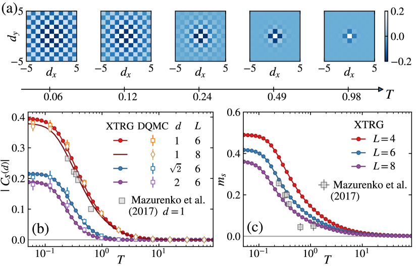
Figure 2: Half-filled Fermi-Hubbard model with $U=7.2$ and sizes $L=4,6,8$. (a) The finite-size AF order pattern is determined from the spin correlation $C_{S}(d)$ versus $(d_{x},d_{y})$, which melts gradually as $T$ increases. We show in (b) the spin correlation function $|C_{S}(d)|$ of various $d=1,\sqrt{2},2$, and in (c) the finite-size spontaneous magnetization $m_{s}$ (see definition in the main text). Excellent agreement between the calculated ($L=8$) data to the experimental data Mazurenko et al. (2017) can be observed.

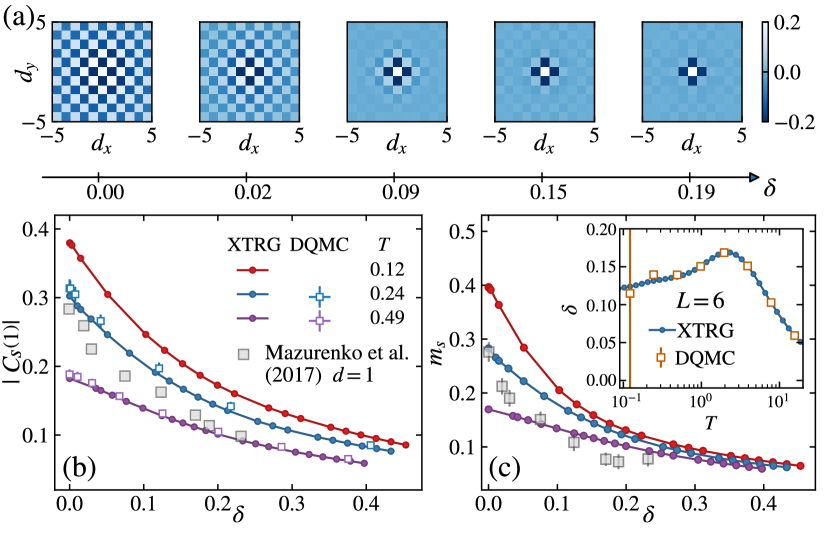
Figure 3: Doped Fermi-Hubbard model with $U=7.2$ and size $L=6$. (a) shows the spin correlation pattern $C_{S}(d)$ versus doping $\delta$, plotted at the lowest temperature $T=0.06$, where the finite-size AF order fades out for $\delta\gtrsim 0.15$. The computed (b) spin correlations $|C_{S}(d=1)|$ and (c) staggered magnetization $m_{s}$ are compared to the experimental data Mazurenko et al. (2017). The XTRG data in (b,c) are obtained via extrapolation $1/D^{*}\to 0$ SM . In the inset of (c), we show how the doping $\delta$, computed by both XTRG and DQMC, varies with $T$ at a fixed chemical potential $\mu=1.5$.

Spin correlations and finite-size magnetic order at half-filling.— In recent experiments, the Fermi-Hubbard antiferromagnet (AF) has been realized in ultracold optical lattices at low effective temperature $T/t<0.4$ Mazurenko et al. (2017). We first benchmark the XTRG method, along with DQMC, with the experimental results of the Fermi-Hubbard model at half-filing. Fig. 2(a) reveals the finite-size AF magnetic structure by showing the spin-spin correlations $C_{S}(d)\equiv\frac{1}{N_{d}}\sum_{|{i}-{j}|=d}\frac{\langle\hat{S}_{i}\cdot\hat{S}_{{j}}\rangle}{S(S+1)}$, summed over all $N_{d}$ pairs of sites $i$ and $j$ with distance $d$, where $i,j$ both denote 2D Cartesian coordinates for the sites in the original square lattice. The real-space spin structure shows AF magnetic order across the finite-size system at low temperature, e.g., $T\lesssim 0.12$, which melts gradually as temperature increases. The AF pattern effectively disappears above $T\sim 0.49$, in good agreement with recent experiments Mazurenko et al. (2017). In Fig. 2(b), we show $|C_{S}(d)|$ vs. $T$ at three fixed values of $d=1,\sqrt{2},2$. Our XTRG and DQMC curves agree rather well in the whole temperature range, for both $L=6$ and 8. Fig. 2(c) shows the spontaneous magnetization $m_{s}\equiv\sqrt{S(\pi,\pi)}$ vs. $T$ for $L=4,6,8$. Here $S(q)=\frac{1}{N(N-1)}\sum^{\prime}_{{i},{j}}\frac{\langle\hat{S}_{i}\cdot\hat{S}_{{j}}\rangle}{S(S+1)}e^{-\mathrm{i}{q}\cdot({i}-{j})}$ is the spin structure factor, where the summation excludes on-site correlations (following the convention from experiments Mazurenko et al. (2017)) and $N=L^{2}$ the total system size. For all system sizes considered, the spontaneous magnetization $m_{s}$ grows quickly as $T$ is decreased from $\simeq 1$ to $\simeq 0.1$. Notably, for both spin correlations and spontaneous magnetization, the $L=8$ XTRG data shows good qualitative agreement with the experimental measurements. This may be ascribed to the similar system sizes and boundary conditions, i.e., $8\times 8$ open square lattices vs. approximately 75-site optical lattice in experiments Mazurenko et al. (2017).

Staggered magnetization upon hole doping.— By tuning the chemical potential $\mu<U/2$, we dope holes into the system and study how they affect the magnetic properties. Fig. 3(a) shows the spin correlation patterns for different dopings $\delta$ at low $T$. The AF order clearly seen at low doping, becomes increasingly short ranged as $\delta$ increases, effectively reduced to nearest-neighbor (NN) only for $\delta\gtrsim 0.15$. The fall-off of AF order upon doping can also be observed in $|C_{S}(d)|$ with a fixed distance $d$. In Fig. 3(b), we show the $d=1$ NN spin correlations. Our XTRG and DQMC agree well for $T=0.49$ and 0.24, while the sign problem hinders DQMC from reaching the lowest $T=0.12$ SM .

Fig. 3(c) shows the staggered magnetization $m_{s}$ vs. $\delta$. Again a rapid drop of the finite-size AF order at approximately $\delta\in[0.1,0.25]$ can be seen. The qualitative agreement with experimental measurements seen in Fig. 3(b,c) suggest that the effective temperature of ultracold fermions falls between $T/t=0.24$ and 0.49, consistent with the experiments Mazurenko et al. (2017). In our calculations we tune the doping $\delta$ by scanning the chemical potentials $\mu$. In the inset of Fig. 3(c), we show the doping $\delta$ vs. $T$ for a fixed $\mu=1.5$ (again the XTRG and DQMC results agree for $T\gtrsim 0.24$ with a tolerable sign problem SM for DQMC). The behavior of $\delta$ is non-monotonic: it first increases as $T$ is lowered [having $\delta(T=\infty)=0$], and then slowly decreases due to hole repulsion (see hole-hole correlation vs. $T$ in SM ).

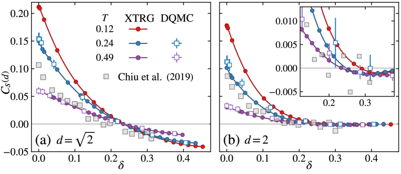
Figure 4: Diagonal and NNN $C_{S}(d)$ correlations as functions of doping $\delta$ for a $6\times 6$ system with $U=7.2$ for (a) $d=\sqrt{2}$ and (b) $d=2$. The inset to (b) zooms in on small $C_{S}(d)$ values. The sign-reversal of $C_{d}$ is in good agreement with experimental data Chiu et al. (2019).

Magnetic polarons.— In Fig. 4, we analyze spin correlations between the diagonal ($d{=}\sqrt{2}$) and next-nearest-neighbor ($d{=}2$, NNN) sites. We compare them to recent measurements where it was found that the diagonal correlation $C_{S}(\sqrt{2})$ undergoes a sign reversal around $\delta\simeq 0.2$ Chiu et al. (2019). Our computations reproduce this fact [Fig. 4(a)]. For the NNN correlations ($d=2$) [Fig. 4(b)], we find that an analogous sign reversal, hardly discernible in experiments, takes place around $\delta\simeq 0.25$.

The sign reversal can be explained within the geometric string theory Grusdt et al. (2018). It signals the formation of a magnetic polaron in the system. As shown in Fig. 1(c), the hole motion through the system generates a string of misaligned spins. The strong NN AF spin correlations are thus mixed with the diagonal and even further correlations, e.g. $C_{S}(2)$, resulting in even ferromagnetic clusters [red and blue shaded regions in Fig. 1(c)]. Due to the interplay between the charge impurity and magnetic background, the moving hole distorts the AF background around the dopant [see the gray “cloud” in Fig. 1(b)], giving rise to a collective excitation, i.e., the magnetic polaron. Such exotic quasi-particles in doped Hubbard system have been imaged experimentally Koepsell et al. (2019) for a doublon in the particle-doped case.

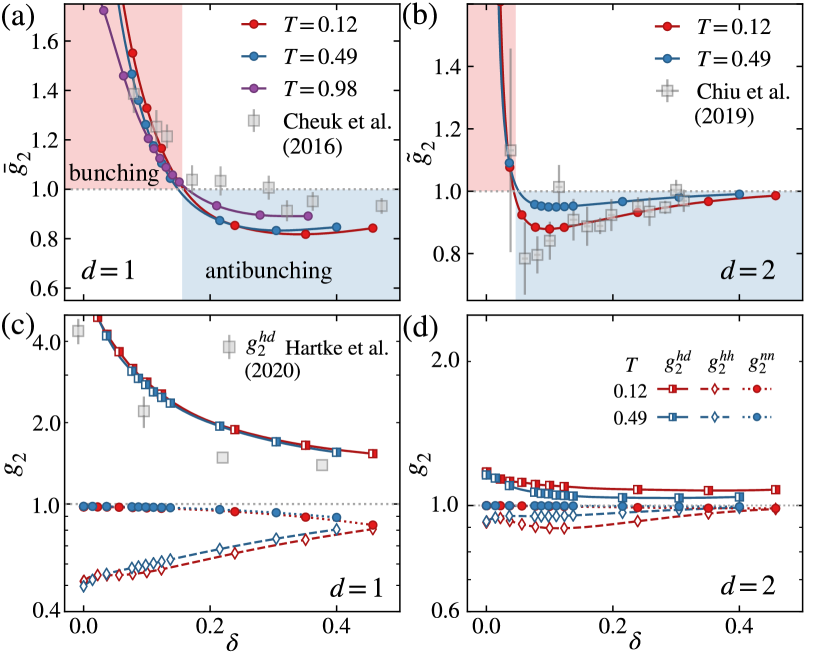
Figure 5: Various $g_{2}$ correlators for a $6\times 6$ system with $U=7.2$. The antimoment correlators (a) $\bar{g}_{2}(d=1)$ and (b) $\tilde{g}_{2}(d=2)$ are shown as functions of doping $\delta$. Experimental data with $d=1$, $T/t\simeq 1.0$ Cheuk et al. (2016b) and $d=2$, $T/t\simeq 0.25$ Chiu et al. (2019) are included for comparison. (c, d) The two-cite hole-doublon ($g_{2}^{hd}$), hole-hole ($g_{2}^{hh}$), and full-density ($g_{2}^{nn}$) correlations, for (c) $d=1$ and (d) $d=2$. The $d=1$ hole-doublon correlations $g_{2}^{hd}$ is compared with experiment in (c), where a nice agreement is observed despite a separate $U/t\simeq 11.8$ in experiment Hartke et al. (2020).

Hole-doublon bunching and hole-hole antibunching.— Quantum gas microscope can also access parity-projected antimoment correlation functions defined in the charge sector, $\bar{g}_{2}(d)\equiv\frac{1}{N_{d}}\sum_{|{i}-{j}|=d}\frac{\langle\hat{\alpha}_{i}\,\hat{\alpha}_{j}\rangle}{\langle\hat{\alpha}_{i}\rangle\langle\hat{\alpha}_{j}\rangle}$ Cheuk et al. (2016b) and $\tilde{g}_{2}\equiv\frac{1}{N_{d}}\sum_{|{i}-{j}|=d}\frac{1}{\delta^{2}}[\langle\hat{\alpha}_{i}\hat{\alpha}_{j}\rangle-\langle\hat{\alpha}_{i}\rangle\langle\hat{\alpha}_{j}\rangle]$ Chiu et al. (2019), with the antimoment projector $\hat{\alpha}_{i}\equiv\hat{h}_{i}+\hat{d}_{i}$ . Fig. 5(a,b) shows the computed antimoment correlation results. Antimoments are bunching ($\bar{g}_{2}>1$) at low doping, yet become antibunching ($\bar{g}_{2}<1$) at large doping, in quantitative agreement with an earlier ⁴⁰K experiment Cheuk et al. (2016b) and a more recent ⁶Li gas measurement Chiu et al. (2019), see Figs. 5(a) and (b), respectively. The antibunching at large doping is attributed to hole repulsion, and the bunching at low-doping to hole-doublon pairs Cheuk et al. (2016b).

Now antimoments contain contributions from both, holes and doublons, yet their individual contributions cannot be distinguished via parity projection measurements Cheuk et al. (2016b); Chiu et al. (2019). XTRG, however, readily yields detailed correlators $g^{ll^{\prime}}_{2}(d)\equiv\frac{1}{N_{d}}\sum_{|\mathbf{i-j}|=d}\tfrac{\langle\hat{l}_{i}\,\hat{l}^{\prime}_{{j}}\rangle}{\langle\hat{l}_{i}\rangle\langle\hat{l}^{\prime}_{j}\rangle}$, with $l\in\{h,d\}$ and $\hat{l}_{i}\in\{\hat{h}_{i},\hat{d}_{i}\}$ for hole or double-occupancy projectors, respectively. Later we also use $l=n$ for $\hat{l}_{j}=\hat{n}_{j}$ the local density.

Our results for the correlations $g_{2}^{hh}(d)$ and $g_{2}^{hd}(d)$ vs. $\delta$ are shown in Fig. 5(c,d). We always find $g_{2}^{hh}(d)<1$ and therefore anticorrelation amongst holes, while $g_{2}^{hd}>1$ corresponds to strong bunching between holes and doublons. As shown in Fig. 5(c), the computed $g_{2}^{hd}$ data show remarkable agreement with very recent experimental measurements using the full-density-resolved bilayer readout technique Hartke et al. (2020); Koepsell et al. (2020). The change from bunching to antibunching behaviors in antimoment correlations in Fig. 5(a,b) can be ascribed to the fact that the hole-doublon attraction is advantageous over the hole-hole repulsion at low doping while the latter dominates at relatively large doping SM . When comparing the charge correlations at $d=1$ and 2 in Fig. 5(c,d), we find that the hole-doublon bunching effect in $\bar{g}_{2}(1)$ is particularly strong at $\delta\ll 1$, where the holes mostly stem from NN hole-doublon pairs [see illustration in Fig. 1(b)]. The further-ranged $g_{2}^{hd}(2)$ still shows the bunching effect, yet gets much reduced.

The full density correlation $g_{2}^{nn}(d)$ is shown in Fig. 5(c, d). We observe $g_{2}^{nn}(d)\approx 1$ at low doping for both $d=1,2$, i.e., weak non-local charge correlations near half-filling, and a more pronounced anti-correlation $g_{2}^{nn}(d)<1$ as $\delta$ increases. Based on our XTRG results, we further reveal that the longer-ranged $g_{2}^{nn}(2)$ also exhibits anticorrelations upon doping, suggesting the statistical Pauli holes may be rather nonlocal, though decaying rapidly spatially.

Conclusion and outlook.— In this work, we generalized XTRG Chen et al. (2018); Li et al. (2019) to the 2D Fermi-Hubbard model. Employing XTRG and DQMC, we obtained reliable results both for half-filling and doped cases and found consistency with the ultracold atom experiments. XTRG can explore a broader parameter space, especially in the doped case, than DQMC, which is limited by a minus-sign problem. XTRG$+$DQMC constitutes a state-of-the-art complimentary numerical setup for probing the phase diagram of Fermi-Hubbard models, for SU(2) fermions here and generally SU(N) fermions Ozawa et al. (2018), thanks to the implementation of non-Abelian symmetries Weichselbaum (2012). Fundamental questions, such as the explanation of the Fermi arcs and the pseudogap phase Norman et al. (1998); Keimer et al. (2015), with their implications for the breaking of Luttinger’s theorem Luttinger (1960); Oshikawa (2000); Paramekanti and Vishwanath (2004); Senthil et al. (2003), or the role of topological order Gazit et al. (2019); Chen et al. (2020, 2020) are open interesting topics to be studied by XTRG$+$DQMC and optical lattices.

Acknowledgments.— B.-B.C. and C.C. contributed equally to this work. The authors are greatly indebted to Fabian Grusdt and Annabelle Bohrdt for numerous insightful discussions. W.L., J.C., C.C. and Z.Y.M. are supported by National Natural Science Foundation of China (Nos. 11974036, 11834014, 11921004, 11904018) and the Fundamental Research Funds for the Central Universities. Z.Y.M. is also supported by the RGC of Hong Kong SAR China (Grant Nos. 17303019 and 17301420). The German Research Foundation (DFG) supported this research through WE4819/3-1 (B.-B.C.) and Germany’s Excellent Strategy – EXC-2111 – 390814868. A.W. was supported by the U.S. Department of Energy, Office of Basic Energy Sciences, under Contract No. DE-SC0012704. We thank the Center for Quantum Simulation Sciences in the Institute of Physics, Chinese Academy of Sciences, the Computational Initiative at the Faculty of Science at the University of Hong Kong, the Tianhe platforms at the National Supercomputer Centers in Tianjin and Guangzhou, and the Leibniz-Rechenzentrum in Munich for their technical support and generous allocation of CPU time.

A A. Exponential Tensor Renormalization Group Approach for Correlated Fermions

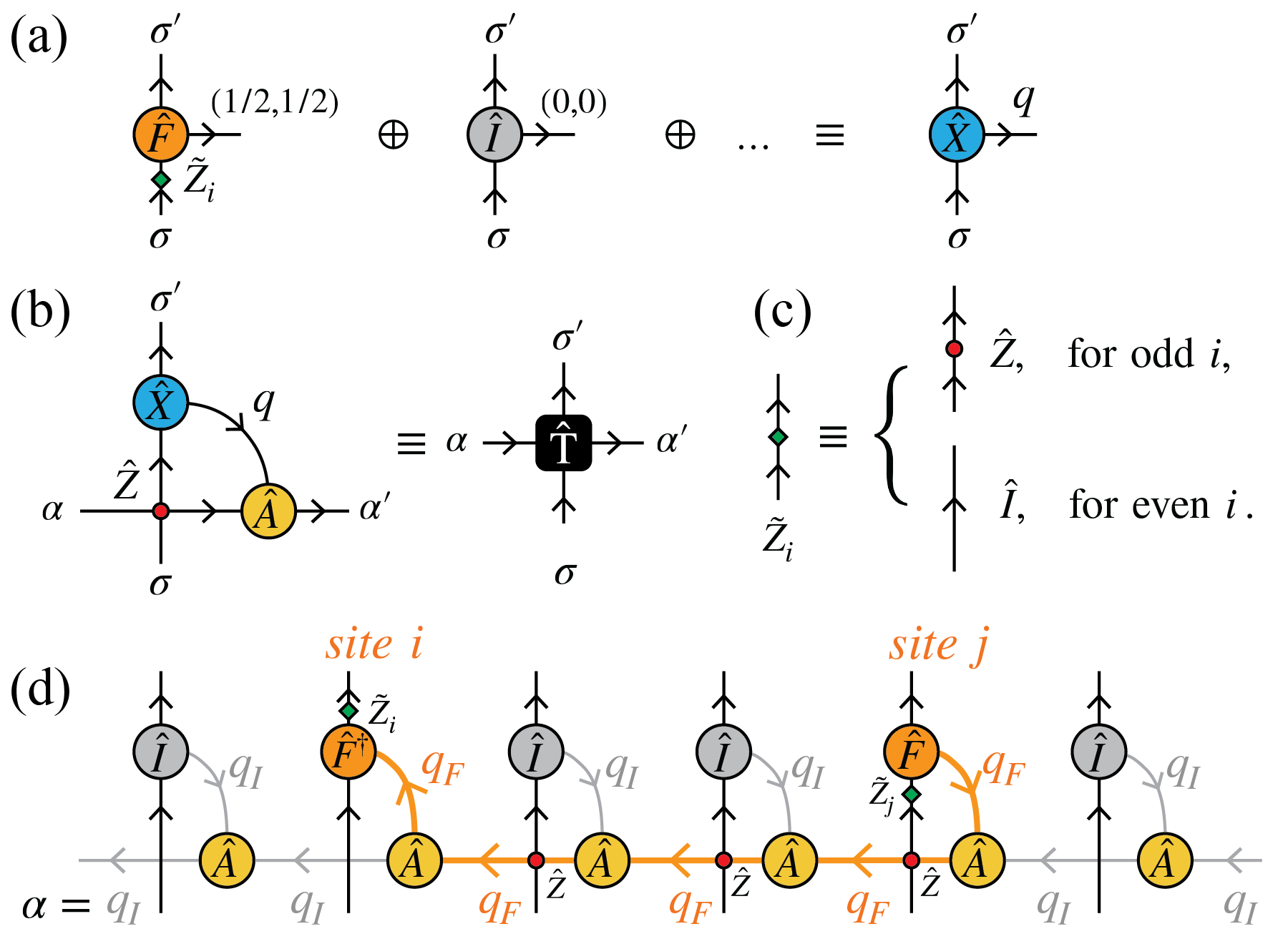
Figure S1: Tensor-network representation for fermion operators. — (a) An irreducible operator (irop) can always be assigned an irop index, shown as the horizontal line sticking out towards the right of a tensor indicated by a circle. The vertical lines describe a local state space. The irop index is also assigned symmetry labels $q\equiv(C,S)$ which describe the transformation of the operator under given charge ($C$) and spin ($S$) symmetry. Here examples of local irops are the fermion operator $\hat{F}$ [with $q_{F}\equiv(1/2,1/2)$] or a trivial identity operator $\hat{I}$ [with $q_{I}\equiv(0,0)$]. These may be combined into the (non-irop) tensor $\hat{X}$ that now describes a (to the extent required) complete local operator basis. (b) For the MPO of the Hamiltonian, the local tensor $T$ is constructed from the local operator basis $\hat{X}$ and the $A$ tensor of a super-MPS, connected by the operator basis indexed by $q$. Fermionic signs are taken are of by the charge parity operator $\hat{Z}\equiv(-1)^{\hat{n}}$ which needs to be applied at every crossing point of lines if negative charge parity can occur on both lines (this is completely analogous, e.g., to the swap gate in fermionic iPEPS Corboz et al. (2010)). It is denoted by the small red dot. (c) When using SU(2) particle-hole symmetry, the local fermion operator is decorated with an additional $\tilde{Z}_{i}$ (denoted by the green diamond), $\hat{F}_{i}\to\tilde{Z}_{i}\hat{F}_{i}$, to recover the correct hopping structure in terms of signs, with $\tilde{Z}_{i}\in\{\hat{I},\hat{Z}\}$ for even (odd) sites $i$, respectively. (d) A single hopping term in the Hamiltonian, i.e., $h_{i,j}\equiv\hat{F}_{i}^{\dagger}\cdot\hat{F}_{j}^{\ }$ from site $j$ to site $i$ is constructed in MPO form from the local tensor as schematically depicted in panel (b). Local terms in the Hamiltonian are also added to the local MPO basis $\hat{X}$ [suggested by the $\oplus\ldots$ in (a)], e.g., with the onsite interaction given by $(\hat{n}_{i}-1)^{2}\equiv\tfrac{4}{3}\hat{C}_{i}^{\dagger}\cdot\hat{C}_{i}^{\ }$, i.e., the Casimir operator in the SU(2)_charge symmetry.

1 1. Renormalization group algorithms for 2D fermion models

Renormalization group numerical methods provide powerful tools tackling fermion many-body problems. Among others, the density-matrix Noack et al. (1994) and tensor-network renormalization group (TRG) Corboz et al. (2010); Kraus et al. (2010); Gu et al. (2010) methods have been developed to simulate fermion models in two dimensions (2D), with focus on the $T=0$ properties, playing an active role in solving the challenging Fermi-Hubbard model at finite doping LeBlanc et al. (2015); Zheng et al. (2017); Qin et al. (2019); Chung et al. (2020).

For $T>0$, thermal TRG algorithms exploits the purification framework in simulating thermodynamics of both infinite- and finite-size systems Verstraete et al. (2004); Zwolak and Vidal (2004); Feiguin and White (2005); Li et al. (2011). Recently, generalizations of DMRG-type calculations to finite temperature have become available via matrix-product-state samplings Bruognolo et al. (2017); Chung and Schollwöck (2019) and the exponential TRG (XTRG) Chen et al. (2018, 2019); Li et al. (2019). Most of the thermal TRG methods mainly apply to the spin/boson systems, and there are few attempts for fermions at finite temperature. For example, an infinite TRG approach has been proposed to simulate 2D fermion lattice models directly in the thermodynamic limit, however it is restricted to relatively high temperature Czarnik and Dziarmaga (2014). Therefore, it is highly desirable to have reliable and accurate TRG algorithms for simulating large-scale correlated fermion systems down to low temperatures.

XTRG can be employed to simulate large-scale system sizes, e.g., width-8 cylinders for the square-lattice Heisenberg model Li et al. (2019), and width-6 cylinders Chen et al. (2019) for the triangular-lattice Heisenberg model, providing full and accurate access to various thermodynamic quantities as well as entanglement and correlations down to low temperature. Here, we generalize XTRG to 2D fermion models and perform the calculations on $L\times L$ open square lattices up to size $L=8$ (half filling) and $L=6$ (finite doping).

2 2. Particle-hole and spin symmetries

In the XTRG calculations of the Fermi-Hubbard model, we implement non-Abelian/Abelian particle-hole and spin symmetries in the matrix-product operator (MPO) representation of the Hamiltonian and the thermal density operators, which greatly reduces the computational resources and makes the high-precision low-temperature simulations possible in XTRG. Here the symmetry implementation is based on the QSpace tensor library Weichselbaum (2012).

To be specific, consider the SU(2)${}_{\rm charge}\otimes$ SU(2)_spin symmetry as an example. The SU(2)_charge, i.e., particle-hole symmetry is present in the Fermi-Hubbard model at half-filling on a bipartite lattices, such as the square lattice considered in this work. QSpace permits to turn symmetries on or off at will, such that either of the symmetries above can also be reduced to smaller ones, such as U(1)_charge or U(1)_spin. This is required for example in the presence of a chemical potential or an external magnetic field, respectively. Throughout, we stick here to the order convention that the charge label comes first, followed by the spin label, i.e., $q=(C,S)$. For SU(2)_charge, the ‘$S_{z}$’ label corresponds to $\tfrac{1}{2}(n_{i}-1)$, that is, one half the local charge relative to half-filling.

The fermion operators can be organized into an irreducible four-component spinor Weichselbaum (2012),

$$\hat{F}_{{i}}^{(1/2,1/2)}=\left(\begin{array}[]{c}s_{i}\hat{c}^{\dagger}_{i\uparrow}\\ \hat{c}_{i\downarrow}\\ s_{i}\hat{c}^{\dagger}_{i\downarrow}\\ -\hat{c}_{i\uparrow}\end{array}\right)\text{ .}$$ (S1)

It is an irop that transforms like $q_{F}=(1/2,1/2)$. Because it consists of multiple components, this results in the third index [depicted as leg to the right in Fig. S1(a)]. The local Hilbert space $\sigma_{(i)}$ of a site $i$ with $d=4$ states can be reduced to $d^{\ast}=2$ multiplets, $q_{\sigma}=(1/2,0)$ combining empty and double occupied, i.e., hole and double states, and $q_{\sigma}=(0,1/2)$ for the local spin $S=1/2$ multiplet at single occupancy.

In Eq. (S1), the index $i\equiv(i_{1},i_{2})$ denotes a 2D Cartesian coordinate of the site in original square lattice. The implementation of SU(2)_charge requires a bipartite lattice, $\mathcal{L}=\mathcal{A}\cup\mathcal{B}$, which we distinguish by the parity $s_{i}=\pm 1$, e.g., choosing arbitrarily but fixed that the sites in $\mathcal{A}$ are even, i.e., have $s_{i}=+1$ for $i\in\mathcal{A}$. In practice, we adopt a snake-like mapping of the 2D square lattice (as shown in Fig. 1), with a 1D site ordering index $i$. This leads to a simple rule: a site with $i\in$ even (odd) site of the quasi-1D chain also corresponds to the even (odd) sublattice of the square lattice with $s_{i}=\pm 1$.

For SU(2)_charge, to recover the correct hopping term in the Hamiltonian, this requires the alternating sign factor $s_{i}$. In fact, this alternating sign can be interpreted as different fermion orderings on the even and odd sites Weichselbaum (2012), i.e.,

$$|\mathbin{\uparrow}\downarrow\rangle_{i} = s_{i}\ \hat{c}^{\dagger}_{i\uparrow}\hat{c}^{\dagger}_{i\downarrow}|0\rangle=\begin{cases}\,\hat{c}^{\dagger}_{i\downarrow}\hat{c}^{\dagger}_{i\uparrow}|0\rangle,&\text{$i\in$ odd, $s_{i}=-1$,}\\ \\ \,\hat{c}^{\dagger}_{i\uparrow}\hat{c}^{\dagger}_{i\downarrow}|0\rangle,&\text{$i\in$ even, $s_{i}=1$.}\end{cases}$$ (S2)

By reversing the fermionic order of every other site for the local state space as above, we thus recover the correct structure in the electron hopping term

$$\hat{h}_{i,j}=\hat{F}_{i}^{\dagger}\cdot\hat{F}_{j}^{\ }=(\hat{c}_{i\uparrow}^{\dagger}\hat{c}_{j\uparrow}^{\ }+\hat{c}_{i\downarrow}^{\dagger}\hat{c}_{j\downarrow}^{\ })+\mathrm{H.c.},$$ (S3)

with site $i$ and $j$ always belonging to different sublattices of the square lattice. By summing over all pairs of hopping terms, we recover the tight-binding (TB) kinetic energy term on the square lattice, whose Hamiltonian reads

$$\hat{H}_{\text{TB}}=\sum_{\langle i,j\rangle}\hat{h}_{i,j}=\sum_{\langle i,j\rangle}\hat{F}_{i}^{\dagger}\cdot\hat{F}_{j}^{\phantom{\dagger}}\text{ .}$$ (S4)

By the structure of a scalar product, Eq. (S4) explicitly reveals the SU(2) particle-hole and spin symmetry.

When the interaction $U$ is turned on, the Fermi-Hubbard Hamiltonian [see Eq. (1) in the main text] remains SU(2)${}_{\rm{charge}}\otimes$SU(2)_spin invariant, as long as half-filling is maintained, i.e., $\mu=U/2$. Then

$$\sum_{i}U\hat{n}_{i\uparrow}\hat{n}_{i\downarrow}-\tfrac{U}{2}(\hat{n}_{i\uparrow}+\hat{n}_{i\downarrow})\equiv\tfrac{U}{2}\sum_{i}(\hat{n}_{i}-1)^{2}+\text{const.}$$

has a SU(2) charge symmetry, and the system has a totally symmetric energy spectrum centered around $C_{z}=0$. It is proportional to the Casimir operator of SU(2)_charge. However, when $\mu\neq U/2$, this acts like a magnetic field in the charge sector, and the SU(2)_charge symmetry is reduced to U(1)_charge.

3 3. Fermionic MPO

Given this symmetric construction of the local fermionic operator $\hat{F}_{i}$ we describe below how to represent the many-body Hamiltonian as a fermionic MPO, by taking the square-lattice tight-binding model Eq. (S4) mentioned above as an example. We first introduce a super matrix product state (super-MPS) representation in Fig. S1, which encode the “interaction” information compactly and can be conveniently transformed into the MPO by contracting the $A$ tensor with the local operator basis $\hat{X}$, as shown in Fig. S1(a,b).

$\|A_{\alpha,\alpha^{\prime}}^{q\,[k]}\|$	$\alpha$	$\alpha^{\prime}$	$q$	$k$
1.	(0,0)	(0,0)	$(0,0)$	$k<i$ or $k>j$
1.	(0,0)	$(\tfrac{1}{2},\tfrac{1}{2})$	$(\tfrac{1}{2},\tfrac{1}{2})$	$k=i$
1.	$(\tfrac{1}{2},\tfrac{1}{2})$	(0,0)	$(\tfrac{1}{2},\tfrac{1}{2})$	$k=j$
1.	$(\tfrac{1}{2},\tfrac{1}{2})$	$(\tfrac{1}{2},\tfrac{1}{2})$	$(0,0)$	$i<k<j$

Table 1: The nonzero reduced tensor elements $\|A_{\alpha,\alpha^{\prime}}^{q\,[k]}\|$ at site $k$ [cf. Fig. S1(d)], in the MPO representation of a specific hopping term $h_{i,j}$ (Eq. S3) between site $i$ and $j$. The indices $\alpha,\alpha^{\prime}$, and $q$ are labeled by symmetry quantum numbers $(C,S)$.

To be specific, consider a single hopping term $h_{i,j}$ between site $i\neq j$ in Fig. S1(d). In the super-MPS, the corresponding $A$ tensors have a simple internal structure, as listed in Tab. 1, since the main purpose of the $A$-tensor is to route lines through. Hence they also contain simple Clebsch Gordan coefficients, with the fully scalar representation $(0,0)$ always at least on one index. In $\|A_{\alpha,\alpha^{\prime}}^{q\,[k]}\|$, $\alpha,\alpha^{\prime}$ can be $q_{\mathrm{F}}=(\tfrac{1}{2},\tfrac{1}{2})$ or $q_{\mathrm{I}}=(0,0)$ as shown in Fig. S1(c). Correspondingly, this contracts with either the fermion operator $\hat{F}$ or $\hat{I}$ in $\hat{X}^{q}$, respectively. Contracting $\hat{X}^{q}$ onto $A$, this casts the super-MPS which is made of $A$-tensors only, into “MPO” form consisting of the rank-4 tensors $T$, as indicated in Fig. S1(b). With the index $\alpha$ routed from site $i$ to site $j$, its $q$-label is fixed to that of the irop. Therefore each single hopping term $h_{i,j}$ can be represented as an MPO as in Fig. S1(d), with reduced bond dimension $D^{*}=1$ (one multiplet per geometric bond). Following a very similar procedure as in XTRG for spin systems Chen et al. (2018), we can thus sum over all $h_{i,j}$ terms and obtain a compact MPO representation of the Hamiltonian Eq. (S4) through variational compression which as part of the initialization is cheap. This guarantees that an MPO with minimal bond dimension $D^{\ast}$ is obtained.

4 4. Fermion parity operator $\hat{Z}$

The $\hat{X}^{q}$ operator basis acts on the local fermionic Hilbert space, and thus fermionic signs need to be accounted for in the construction of the MPO representation of the Hamiltonian. As shown in Fig. S1(d), we introduce a product of parity operators $\hat{Z}$ between site $i$ and $j$, generating a Jordan-Wigner string connecting the operators $\hat{F}_{i}^{\dagger}$ and $\hat{F}_{j}$. The parity operator $\hat{Z}$ is defined as $(-1)^{2C+1}$ for any state space, which yields $z=+1$ if $C$ is half-integer (e.g., $C=1/2$ for empty and double occupied), and $z=-1$, otherwise (e.g. $C=0$ for a singly occupied site). In practice, for SU(2)_charge, based on Eq. (S1) we use for even sites ($s_{i}=+1$)

$$\hat{F}\equiv\hat{F}_{\text{even}}^{(1/2,1/2)}=\left(\begin{array}[]{c}\hat{c}^{\dagger}_{i\uparrow}\\ \hat{c}_{i\downarrow}\\ \hat{c}^{\dagger}_{i\downarrow}\\ -\hat{c}_{i\uparrow}\end{array}\right),$$ (S5)

while for odd sites, we use (purely in terms of matrix elements) in the MPO, $\hat{F}_{\mathrm{odd}}=\hat{Z}\hat{F}$, instead (cf. discussion with Eq. (S2); Weichselbaum (2012)), with the Hermitian conjugate $(\hat{Z}\hat{F})^{\dagger}=\hat{F}^{\dagger}\hat{Z}$. Therefore introducing $\tilde{Z}_{i}\in\{\hat{I},\hat{Z}\}$ for even (odd) sites $i$, respectively, this takes care of the alternating sign structure, as illustrated in Fig. S1(c), and consistent with Eq. (S1).

Overall, assuming $i<j$ with similar Fermionic order in that site $i$ is added to the many body state space before site $j$, the hopping term $\hat{h}_{i,j}$ can thus be represented as

$$\hat{h}_{i,j}=(\hat{F}^{\dagger}\tilde{Z})_{i}\otimes\hat{Z}_{i+1}\otimes...\otimes\hat{Z}_{j-1}\otimes(\hat{Z}\tilde{Z}\hat{F})_{j}.$$ (S6)

Given the bipartite lattice structure, therefore up to the dagger, the same $\hat{F}$ (or $\hat{Z}\hat{F}$) is applied at both sites $i$ and $j$ depending on whether $i$ is even (or odd), respectively.

5 5. Exponential cooling and expectation values

XTRG requires the MPO of the Hamiltonian as input for initialization. Therefore when building the MPO for the Hamiltonian, this is the only place where fermionic signs play a role. Thereafter XTRG follows an automated machinery. We compute the thermal density operator $\hat{\rho}(\beta/2)$, and then estimate thermodynamics quantities, entanglement, and correlations from it. We start with a very high-$T$ density operator $\hat{\rho}_{0}(\tau)$ at inverse temperature $\tau\ll 1$, obtained via the series expansion Chen et al. (2017)

$$\hat{\rho}_{0}(\tau)=\sum_{k}\tfrac{(-\tau)^{k}}{k!}\hat{H}^{k}.$$

Here the initial $\tau$ can be exponential small, which thus limits the series expansion to very few terms to already reach machine precision for the initial $\hat{\rho}_{0}(\tau)$. Then, we cool down the system exponentially by squaring the density matrix. The $n$-th XTRG iteration yields

$$\hat{\rho}_{n-1}(2^{n}\tau)\otimes\hat{\rho}_{n-1}(2^{n}\tau)\rightarrow\hat{\rho}_{n}(2^{n+1}\tau).$$ (S7)

With $\hat{\rho}_{n}(2^{n+1}\tau)$, we can compute thermal expectation values at inverse temperatures $\beta_{n}=2^{n+2}\tau$ using the thermofield double trick of purification Feiguin and White (2005); Dong et al. (2017); Chen et al. (2018), equivalent to the simple procedure in Fig. 1.

One advantage in the fermion XTRG is its simplicity. In the cooling step $\hat{\rho}_{n-1}\otimes\hat{\rho}_{n-1}\rightarrow\hat{\rho}_{n}$ in Eq. (S7), no fermion parity operators $\hat{Z}$ are involved when we perform MPO iteration and compression just as for spin/boson systems. Besides, in the calculations of density-density correlations such as spin-spin and hole-hole(-doublon) correlations, the charge quantum numbers $C$ in the $q$-label of operators $\hat{S}$ and $\hat{h}$ ($\hat{d}$) are always even, and thus the Jordan-Wigner string consists of trivial identity operators and can also be safely ignored, as illustrated in Fig. 1(a) of the main text. Even though not required here, also fermionic correlations can be computed within fermionic XTRG, and proceeds completely analogous to fermionic MPS expectation values, then also with a Jordan Wigner string stretching in between sites $i$ and $j$.

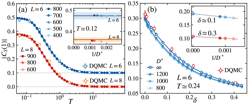
Figure S2: XTRG$+$DQMC bechmark results. (a) NN spin correlation $|C_{S}(d=1)|$ of half-filled square-lattice Hubbard system for $U=7.2$ and sizes $L=6,8$, with $D^{\ast}=400$-$900$. The $L=6$ data have been shifted upwards by 0.1, for the sake of readability. In the inset, $|C_{S}|$ at low temperature $T\simeq 0.12$ is shown versus $1/D^{\ast}$, with the DQMC results [mean (line) and standard deviation (color matched shaded region)] provided. (b) Upon doping, $|C_{S}(1)|$ is shown as a function of $\delta$ for $L=6$ system at $T\simeq 0.24$ (the lowest temperature reachable by DQMC, before the sign problem becomes prohibitive; cf. Fig. S6), with $D^{\ast}=800$-$1200$. Linear extrapolations $1/D^{\ast}\to 0$ are performed, with the extrapolation values depicted as asterisk symbols. The detailed extrapolations at $\delta\simeq 0.1,0.3$ are shown in the inset. In both panels, the DQMC results are also shown for comparison as depicted by the square symbols.

B B. Convergency check and extrapolation

Here we provide detailed convergency check of the spin correlation functions shown in the main text. In Fig. S2(a), at half filled cases, we show the spin correlation function $C_{S}(d=1)$ for different system size $L=6,8$, versus temperature $T$ with various bond dimensions $D^{*}=400$-$900$. For better readability, $C_{S}$ is shifted upwards by 0.1, for $L=6$ system. As shown, in the whole temperature regime, for both $L=6,8$ systems, all $C_{S}$ curves lie on top of each other, showing good agreement with the DQMC data. In the inset, $C_{S}$ at a low temperature $T\simeq 0.12$ are collected at various $D^{\ast}$, showing excellent convergency versus $1/D^{\ast}$. In Fig. S2(b), $|C_{S}(d=1)|$ is shown as a function of hole doping $\delta$ for $L=6$ system, with $D^{\ast}=800$-$1200$, at $T\simeq 0.24$. At each doping rate, the XTRG data exhibit good linearity with $1/D^{\ast}$, enabling us to perform a linear extrapolation to $1/D^{\ast}=0$. As shown, the extrapolation value shows good qualitative agreement with the DQMC results. In the inset, the detailed extrapolations $1/D^{\ast}\to 0$ at around $\delta\simeq 0.1$ and $\delta\simeq 0.3$ are provided.

C C. Charge Correlations in the Doped Fermi-Hubbard Model

1 1. Hole-hole and hole-doublon correlations

In this section, we provide more results on charge correlations

$$C_{hl}(d)=\tfrac{1}{N_{d}}\sum_{|{i}-{j}|=d}\langle\hat{h}_{i}\hat{l}_{j}\rangle-\langle\hat{h}_{i}\rangle\langle\hat{l}_{j}\rangle,$$ (S8)

with $l\in\{h,d\}$ corresponding to $\hat{l}\in\{\hat{h},\hat{d}\}$, where $\hat{h}_{i}\equiv|0\rangle\langle 0|$ and $\hat{d}_{i}\equiv\left|\uparrow\downarrow\rangle\langle\uparrow\downarrow\right|$ are projectors into the empty and double occupied states, respectively. We consider a $6\times 6$ system and set $\mu=1.5$ throughout.

Figure S3(a) shows the hole-hole correlation $C_{hh}$ plotted versus $d_{x}$ and $d_{y}$ from low (left) to high temperatures (right). There clearly exists a non-local anticorrelation in the spatial distribution, having $C_{hh}\leq 0$ throughout, and decays roughly exponentially with distance for any fixed $T$ [Fig. S3(b)]. When plotted vs. $T$ as in Fig. S3(c), the hole-hole anticorrelation persists to relatively high temperature [$T\lesssim 2$], beyond which it rapidly decays to zero. Note also that around $T\simeq 2$ for given fixed $\mu=1.5$, a maximal doping $\delta\simeq 0.17$ is reached [see Fig. 3(c) in the main text]. This appears naturally related to the energy scale of the half-bandwidth $2t=2$ for the kinetic energy of the 2D square lattice (ignoring the chemical potential since $\delta\ll 1$).

Figure S3: Hole-hole correlation at doped cases. (a) Hole-hole correlation $C_{hh}(d)$, plotted as function of displacement $d_{x},d_{y}$ along the horizontal and vertical directions, at various temperatures, for $6\times 6$ system at fixed $\mu=1.5$ ($U=7.2$). (b) $C_{hh}(d)$ vs. $d$ at various temperatures, and (c) $C_{hh}(d)$ vs. $T$ for various distances $d=1,\sqrt{2},2$.

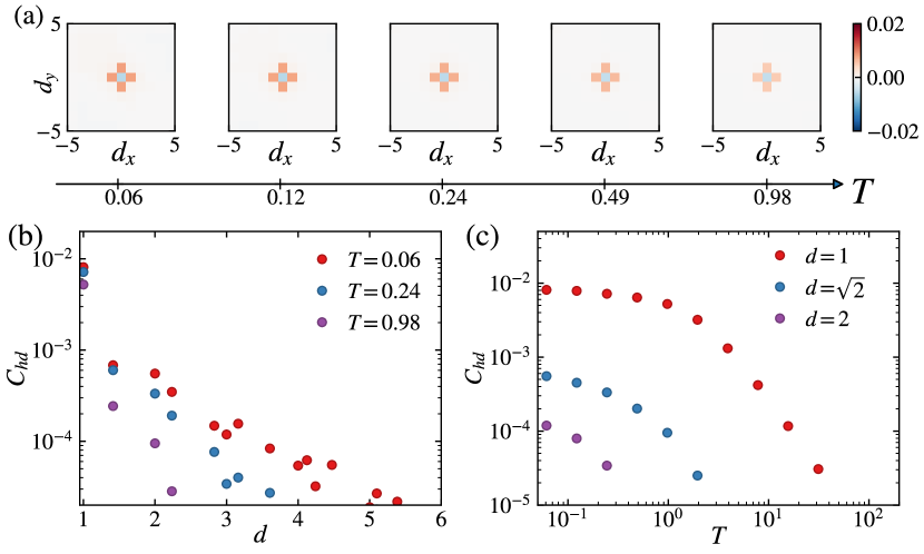
Figure S4: Hole-doublon correlation at doped cases. Same layout as in Fig. S3 otherwise.

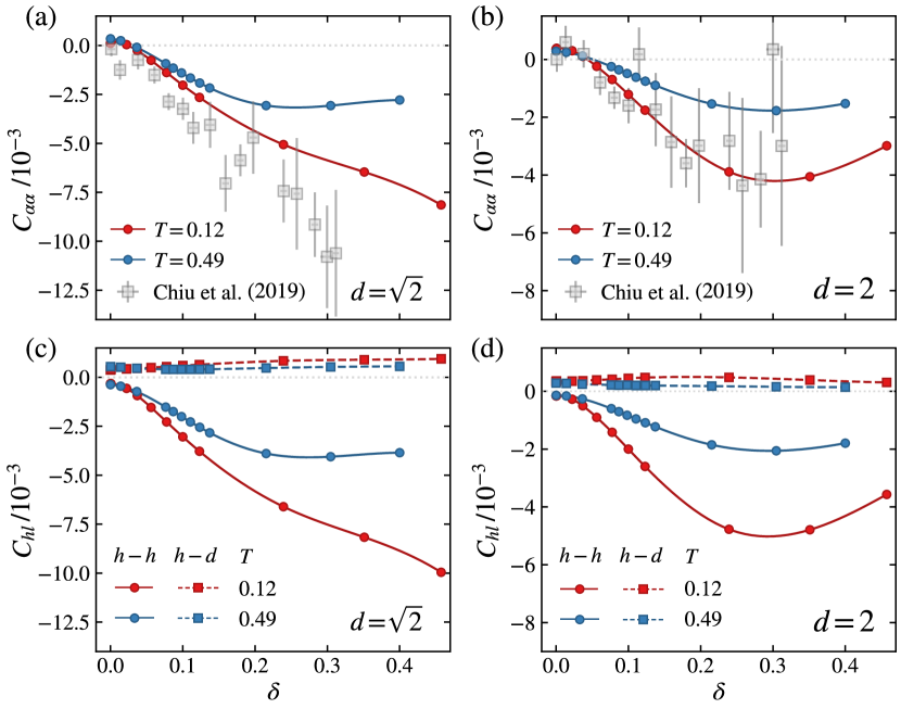
Figure S5: Antimoment correlation functions. The antimoment correlations $C_{\alpha\alpha}(d)$ with (a) $d=\sqrt{2}$ and (b) $d=2$ are shown vs. $\delta$ at two different temperatures $T=0.12$ and $0.49$. The experimental data at $T/t\simeq 0.25$ are also shown for comparison. The hole-hole (‘h-h’) and hole-doublon (‘h-d’) correlation function $C_{hl}$ with (c) $d=\sqrt{2}$ and (d) $d=2$ are shown versus doping $\delta$. The results are computed on a $6\times 6$ square lattice ($U=7.2$).

A completely analogous analysis is performed for the hole-doublon correlations $C_{hd}$ as showns in Fig. S4. Figure S4(a) shows $C_{hd}$ vs. $d_{x}$ and $d_{y}$ at various temperatures, where we observe nonlocal correlations between the hole-doublon pairs. Figure S4(b,c) shows that $C_{hd}$ decays rapidly with increasing distance $d$, and the hole-doublon correlation again persist to a relatively high temperature $T\sim 2$. Overall, the results in Figs. S3 and S4 show that the repulsive hole-hole and attractive hole-doublon pairs are mainly limited to nearest-neighboring sites, as expected given the sizable Coulomb interaction $U=7.2$.

2 2. Antimoment correlations

In this section, we provide the results of antimoment correlation,

$$C_{\alpha\alpha}(d) = \tfrac{1}{N_{d}}\sum_{|i-j|=d}{\langle\hat{\alpha}_{i}\hat{\alpha}_{j}\rangle}-{\langle\hat{\alpha}_{i}\rangle\langle\hat{\alpha}_{j}\rangle}$$ (S9a)

$$= C_{hh}+2C_{hd}+C_{dd}\text{ ,}$$ (S9b)

with $\hat{\alpha}_{i}\equiv\hat{h}_{i}+\hat{d}_{i}$. This can be directly compared with existing experimental data Chiu et al. (2019) for $d=\sqrt{2}$ and $d=2$. Figure S5(a,b) shows $C_{\alpha\alpha}$ vs. doping $\delta$, where a qualitative agreement with the experimental data can be observed. In both Fig. S5(a,b), near half-filling a weak bunching effect is present. Thereafter the antimoments soon exhibit strong anti-bunching effect as one dopes some holes into the system ($\delta\gtrsim 3\%$ for $d=\sqrt{2}$ and $\delta\gtrsim 5\%$ for $d=2$).

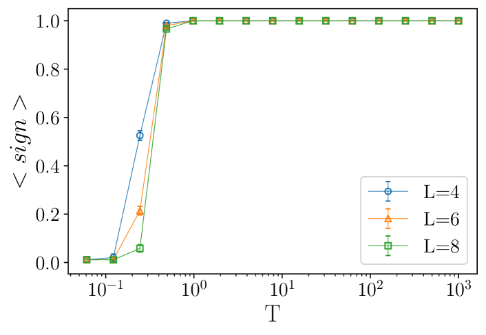
Figure S6: DQMC average sign versus lattice size $L$ and temperature $T$. In the calculations, the chemical potential is fixed at $\mu=1.5$, which corresponds to the data of Fig. 3 in the main text.

Within XTRG, we can also compute all the partial contributions to the antimoment correlations as in Eq. (S9b). The doublon-doublon correlation $C_{dd}$ is negligibly small due to the rare density of doublons considering hole-doping for large $U=7.2$. We thus only provide the results of $C_{hh}(d)$ and $C_{hd}(d)$ vs. doping in Fig. S5(c,d). Over the entire hole-doping regime considered in the present work, the hole-hole correlation $C_{hh}(d)$ exhibits antibunching while the hole-doublon correlation $C_{hd}(d)$ exhibits bunching, for both $d=\sqrt{2}$ in Fig. S5(c) and $d=2$ in Fig. S5(d).

In the vicinity of half-filling, i.e., at low doping, the hole-hole correlation $C_{hh}$ in Fig. S5(c,d) becomes smaller (in absolute values) as compared to the hole-doublon $C_{hd}>0$. This is responsible for the bunching of antimoments at low doping [Fig. S5(a,b)]. However, when more holes are doped into the system, e.g., $\delta\gtrsim 5$ % as shown in Fig. S5, the hole-hole repulsion becomes predominant and thus leads to the overall antibunching of antimoments.

D D. DQMC simulation and average sign in the doped cases

We investigate the 2D square lattice Hubbard model with determinantal QMC simulations. The quartic term in Eq. (1) of the main text,

$$U\hat{n}_{i\uparrow}\hat{n}_{i\downarrow}=-\frac{U}{2}(\hat{n}_{i\uparrow}-\hat{n}_{i\downarrow})^{2}+\frac{U}{2}(\hat{n}_{i\uparrow}+\hat{n}_{i\downarrow})$$

is decoupled by a Hubbard-Stratonovich transformation to a form quadratic in $(\hat{n}_{i\uparrow}-\hat{n}_{i\downarrow})=(\hat{c}^{\dagger}_{i\uparrow}\hat{c}_{i\uparrow}^{\ }-\hat{c}^{\dagger}_{i\downarrow}c_{i\downarrow}^{\ })$ coupled to an auxiliary Ising field on each lattice site Blankenbecler et al. (1981). The particular decomposition above has the advantage that the auxiliary fields can be chosen real. The DQMC procedure obtains the partition function of the underlying Hamiltonian in a path integral formulation in a space of dimension $N=L\times L$ and an imaginary time $\tau$ up to $\beta=1/T$. The auxiliary Ising field lives on the $L\times L\times\beta$ space-time configurational space and each specific configuration gives rise to one term in the configurational sum of the partition function. All of the physical observables are measured from the ensemble average over the space-time ($N\beta$) configurational weights of the auxiliary fields. As a consequence, the errors within the process are well controlled; specifically, the $(\Delta\tau)^{2}$ systematic error from the imaginary-time discretization, $\Delta\tau=\beta/M$, is controlled by the extrapolation $M\to\infty$ and the statistical error is controlled by the central-limit theorem.

The DQMC algorithm employed in this work is based on Ref. Blankenbecler et al. (1981) and has been refined by including global moves to improve ergodicity and delay updating of the fermion Green function. This improves the efficiency of the Monte Carlo sampling Assaad and Evertz (2008). We have performed simulations for system sizes $L=4,6,8$. The interaction is set as $U=7.2$ and we simulate temperatures from $T=0.061$ to 1000 (inverse temperatures $\beta=0.001$ to $16.39$).

We comment briefly on the sign problem in the Monte Carlo sampling which becomes pronounced at finite doping. In general, the computational complexity in the presence of minus sign grows exponentially in the space-time volume $N\beta$. This is because the correct physical observable now must include the effect of the sign of each Monte Carlo weight. One common practice is to use the absolute value of the weight to continue the Monte Carlo simulation, and then the expectation value becomes $\langle\hat{O}\rangle=\frac{\langle\hat{O}\cdot sign\rangle}{\langle sign\rangle}.$

Since the expectation value of the averaged sign, $\langle sign\rangle$, scales as $e^{-\beta N}$, one cannot further extrapolate to the thermodynamic limit in this manner, as the error bar of any physical observables will explode. However, for finite size systems as investigated in this work, there is no problem of performing DQMC and obtaining unbiased results before $\langle sign\rangle$ becomes too small. As shown in Fig. S6, for our system sizes $L=4,6,8$ at chemical potential of $\mu=1.5$ [cf. Fig. 3 (c) of the main text], the average sign is still affordable down to $T=0.244$ for $L=6,8$ [cf. Fig. S2(b)].

Other DQMC parameters of the doped case, with minus sign problem in the main text, are investigated in a similar manner before the average sign becomes too small.

References

- Hubbard and Flowers (1963) J. Hubbard and B. H. Flowers, “Electron correlations in narrow energy bands,” Proceedings of the Royal Society of London. Series A. Mathematical and Physical Sciences 276, 238–257 (1963).
- Gutzwiller (1963) M. C. Gutzwiller, “Effect of Correlation on the Ferromagnetism of Transition Metals,” Phys. Rev. Lett. 10, 159–162 (1963).
- Lee et al. (2006) P. A. Lee, N. Nagaosa, and X.-G. Wen, “Doping a mott insulator: Physics of high-temperature superconductivity,” Rev. Mod. Phys. 78, 17–85 (2006).
- Fazekas (1999) P. Fazekas, Lecture Notes on Electron Correlation and Magnetism, Series In Modern Condensed Matter Physics (World Scientific Publishing Company, 1999).
- Sachdev (2011) S. Sachdev, Quantum Phase Transitions (Cambridge University Press, 2011).
- Wen (2004) X.G. Wen, Quantum Field Theory of Many-Body Systems: From the Origin of Sound to an Origin of Light and Electrons, Oxford Graduate Texts (OUP Oxford, 2004).
- Georges et al. (2013) A. Georges, L. de’ Medici, and J. Mravlje, “Strong correlations from Hund’s coupling,” Annual Review of Condensed Matter Physics 4, 137–178 (2013).
- Bakr et al. (2009) W. S. Bakr, J. I. Gillen, A. Peng, S. Fölling, and M. Greiner, “A quantum gas microscope for detecting single atoms in a Hubbard-regime optical lattice,” Nature 462, 74–77 (2009).
- Parsons et al. (2015) M. F. Parsons, F. Huber, A. Mazurenko, C. S. Chiu, W. Setiawan, K. Wooley-Brown, S. Blatt, and M. Greiner, “Site-resolved imaging of fermionic in an optical lattice,” Phys. Rev. Lett. 114, 213002 (2015).
- Greif et al. (2016) D. Greif, M. F. Parsons, A. Mazurenko, C. S. Chiu, S. Blatt, F. Huber, G. Ji, and M. Greiner, “Site-resolved imaging of a fermionic Mott insulator,” Science 351, 953–957 (2016).
- Boll et al. (2016) M. Boll, T. A. Hilker, G. Salomon, A. Omran, J. Nespolo, L. Pollet, I. Bloch, and C. Gross, “Spin- and density-resolved microscopy of antiferromagnetic correlations in Fermi-Hubbard chains,” Science 353, 1257–1260 (2016).
- Cheuk et al. (2016a) L. W. Cheuk, M. A. Nichols, K. R. Lawrence, M. Okan, H. Zhang, and M. W. Zwierlein, “Observation of 2D fermionic Mott insulators of with single-site resolution,” Phys. Rev. Lett. 116, 235301 (2016a).
- Cheuk et al. (2016b) L. W. Cheuk, M. A. Nichols, K. R. Lawrence, M. Okan, H. Zhang, E. Khatami, N. Trivedi, T. Paiva, M. Rigol, and M. W. Zwierlein, “Observation of spatial charge and spin correlations in the 2D Fermi-Hubbard model,” Science 353, 1260–1264 (2016b).
- Parsons et al. (2016) M. F. Parsons, A. Mazurenko, C. S. Chiu, G. Ji, D. Greif, and M. Greiner, “Site-resolved measurement of the spin-correlation function in the Fermi-Hubbard model,” Science 353, 1253–1256 (2016).
- Greif et al. (2013) D. Greif, T. Uehlinger, G. Jotzu, L. Tarruell, and T. Esslinger, “Short-Range Quantum Magnetism of Ultracold Fermions in an Optical Lattice,” Science 340, 1307–1310 (2013).
- Hart et al. (2015) R. A. Hart, P. M. Duarte, T.-L. Yang, X. Liu, T. Paiva, E. Khatami, R. T. Scalettar, N. Trivedi, D. A. Huse, and R. G. Hulet, “Observation of antiferromagnetic correlations in the hubbard model with ultracold atoms,” Nature 519, 211–214 (2015).
- Mazurenko et al. (2017) A. Mazurenko, C. S. Chiu, G. Ji, M. F. Parsons, M. Kanász-Nagy, R. Schmidt, F. Grusdt, E. Demler, D. Greif, and M. Greiner, “A cold-atom Fermi–Hubbard antiferromagnet,” Nature 545, 462–466 (2017).
- Brown et al. (2017) P. T. Brown, D. Mitra, E. Guardado-Sanchez, P. Schauß, S. S. Kondov, E. Khatami, T. Paiva, N. Trivedi, D. A. Huse, and W. S. Bakr, “Spin-imbalance in a 2D Fermi-Hubbard system,” Science 357, 1385–1388 (2017).
- Hilker et al. (2017) T. A. Hilker, G. Salomon, F. Grusdt, A. Omran, M. Boll, E. Demler, I. Bloch, and C. Gross, “Revealing hidden antiferromagnetic correlations in doped Hubbard chains via string correlators,” Science 357, 484–487 (2017).
- Chiu et al. (2019) C. S. Chiu, G. Ji, A. Bohrdt, M. Xu, M. Knap, E. Demler, F. Grusdt, M. Greiner, and D. Greif, “String patterns in the doped Hubbard model,” Science 365, 251–256 (2019).
- Salomon et al. (2019) G. Salomon, J. Koepsell, J. Vijayan, T. A. Hilker, J. Nespolo, L. Pollet, I. Bloch, and C. Gross, “Direct observation of incommensurate magnetism in Hubbard chains,” Nature 565, 56–60 (2019).
- Koepsell et al. (2019) J. Koepsell, J. Vijayan, P. Sompet, F. Grusdt, T. A. Hilker, E. Demler, G. Salomon, I. Bloch, and C. Gross, “Imaging magnetic polarons in the doped Fermi–Hubbard model,” Nature 572, 358–362 (2019).
- Nichols et al. (2019) M. A. Nichols, L. W. Cheuk, M. Okan, T. R. Hartke, E. Mendez, T. Senthil, E. Khatami, H. Zhang, and M. W. Zwierlein, “Spin transport in a Mott insulator of ultracold fermions,” Science 363, 383–387 (2019).
- Brown et al. (2019) P. T. Brown, D. Mitra, E. Guardado-Sanchez, R. Nourafkan, A. Reymbaut, C.-D. Hébert, S. Bergeron, A.-M. S. Tremblay, J. Kokalj, D. A. Huse, P. Schauß, and W. S. Bakr, “Bad metallic transport in a cold atom Fermi-Hubbard system,” Science 363, 379–382 (2019).
- Hartke et al. (2020) T. Hartke, B. Oreg, N. Jia, and M. Zwierlein, “Measuring total density correlations in a Fermi-Hubbard gas via bilayer microscopy,” arXiv e-prints (2020), arXiv:2003.11669 .
- Chen et al. (2013) K.-S. Chen, Z. Y. Meng, S.-X. Yang, T. Pruschke, J. Moreno, and M. Jarrell, “Evolution of the superconductivity dome in the two-dimensional hubbard model,” Phys. Rev. B 88, 245110 (2013).
- Noack et al. (1994) R. M. Noack, S. R. White, and D. J. Scalapino, “The Density Matrix Renormalization Group for Fermion Systems,” arXiv e-prints (1994), arXiv:cond-mat/9404100 .
- Corboz et al. (2010) P. Corboz, R. Orús, B. Bauer, and G. Vidal, “Simulation of strongly correlated fermions in two spatial dimensions with fermionic projected entangled-pair states,” Phys. Rev. B 81, 165104 (2010).
- Kraus et al. (2010) C. V. Kraus, N. Schuch, F. Verstraete, and J. I. Cirac, “Fermionic projected entangled pair states,” Phys. Rev. A 81, 052338 (2010).
- Gu et al. (2010) Z.-C. Gu, F. Verstraete, and X.-G. Wen, “Grassmann tensor network states and its renormalization for strongly correlated fermionic and bosonic states,” arXiv e-prints (2010), arXiv:1004.2563 .
- LeBlanc et al. (2015) J. P. F. LeBlanc, A. E. Antipov, F. Becca, I. W. Bulik, G. K.-L. Chan, C.-M. Chung, Y. Deng, M. Ferrero, T. M. Henderson, C. A. Jiménez-Hoyos, E. Kozik, X.-W. Liu, A. J. Millis, N. V. Prokof’ev, M. Qin, G. E. Scuseria, H. Shi, B. V. Svistunov, L. F. Tocchio, I. S. Tupitsyn, S. R. White, S. Zhang, B.-X. Zheng, Z. Zhu, and E. Gull (Simons Collaboration on the Many-Electron Problem), “Solutions of the two-dimensional hubbard model: Benchmarks and results from a wide range of numerical algorithms,” Phys. Rev. X 5, 041041 (2015).
- Zheng et al. (2017) B.-X. Zheng, C.-M. Chung, P. Corboz, G. Ehlers, M.-P. Qin, R. M. Noack, H. Shi, S. R. White, S. Zhang, and G. K.-L. Chan, “Stripe order in the underdoped region of the two-dimensional Hubbard model,” Science 358, 1155–1160 (2017).
- Qin et al. (2019) M. Qin, C.-M. Chung, H. Shi, E. Vitali, C. Hubig, U. Schollwöck, S. R. White, and S. Zhang, “Absence of superconductivity in the pure two-dimensional Hubbard model,” arXiv e-prints , arXiv:1910.08931 (2019), arXiv:1910.08931 .
- Chung et al. (2020) C.-M. Chung, M. Qin, S. Zhang, U. Schollwöck, and S. R. White, “Plaquette versus ordinary -wave pairing in the -Hubbard model on a width 4 cylinder,” arXiv e-prints , arXiv:2004.03001 (2020), arXiv:2004.03001 .
- Chen et al. (2018) B.-B. Chen, L. Chen, Z. Chen, W. Li, and A. Weichselbaum, “Exponential Thermal Tensor Network Approach for Quantum Lattice Models,” Phys. Rev. X 8, 031082 (2018).
- Li et al. (2019) H. Li, B.-B. Chen, Z. Chen, J. von Delft, A. Weichselbaum, and W. Li, “Thermal tensor renormalization group simulations of square-lattice quantum spin models,” Phys. Rev. B 100, 045110 (2019).
- Han et al. (2019) X.-J. Han, C. Chen, J. Chen, H.-D. Xie, R.-Z. Huang, H.-J. Liao, B. Normand, Z. Y. Meng, and T. Xiang, “Finite-temperature charge dynamics and the melting of the Mott insulator,” Phys. Rev. B 99, 245150 (2019).
- Varney et al. (2009) C. N. Varney, C.-R. Lee, Z. J. Bai, S. Chiesa, M. Jarrell, and R. T. Scalettar, “Quantum Monte Carlo study of the two-dimensional fermion Hubbard model,” Phys. Rev. B 80, 075116 (2009).
- Verstraete et al. (2004) F. Verstraete, J. J. García-Ripoll, and J. I. Cirac, “Matrix product density operators: Simulation of finite-temperature and dissipative systems,” Phys. Rev. Lett. 93, 207204 (2004).
- Zwolak and Vidal (2004) M. Zwolak and G. Vidal, “Mixed-state dynamics in one-dimensional quantum lattice systems: A time-dependent superoperator renormalization algorithm,” Phys. Rev. Lett. 93, 207205 (2004).
- Feiguin and White (2005) A. E. Feiguin and S. R. White, “Finite-temperature density matrix renormalization using an enlarged hilbert space,” Phys. Rev. B 72, 220401 (2005).
- Li et al. (2011) W. Li, S.-J. Ran, S.-S. Gong, Y. Zhao, B. Xi, F. Ye, and G. Su, “Linearized tensor renormalization group algorithm for the calculation of thermodynamic properties of quantum lattice models,” Phys. Rev. Lett. 106, 127202 (2011).
- Chen et al. (2017) B.-B. Chen, Y.-J. Liu, Z. Chen, and W. Li, “Series-expansion thermal tensor network approach for quantum lattice models,” Phys. Rev. B 95, 161104 (2017).
- Bruognolo et al. (2017) B. Bruognolo, Z. Zhu, S. R. White, and E. Miles Stoudenmire, “Matrix product state techniques for two-dimensional systems at finite temperature,” arXiv e-prints , arXiv:1705.05578 (2017), arXiv:1705.05578 .
- Chung and Schollwöck (2019) C.-M. Chung and U. Schollwöck, “Minimally entangled typical thermal states with auxiliary matrix-product-state bases,” arXiv e-prints , arXiv:1910.03329 (2019), 1910.03329 .
- Khatami and Rigol (2011) E. Khatami and M. Rigol, “Thermodynamics of strongly interacting fermions in two-dimensional optical lattices,” Phys. Rev. A 84, 053611 (2011).
- Czarnik and Dziarmaga (2014) P. Czarnik and J. Dziarmaga, “Fermionic projected entangled pair states at finite temperature,” Phys. Rev. B 90, 035144 (2014).
- Dong et al. (2017) Y.-L. Dong, L. Chen, Y.-J. Liu, and W. Li, “Bilayer linearized tensor renormalization group approach for thermal tensor networks,” Phys. Rev. B 95, 144428 (2017).
- Chen et al. (2019) L. Chen, D.-W. Qu, H. Li, B.-B. Chen, S.-S. Gong, J. von Delft, A. Weichselbaum, and W. Li, “Two-temperature scales in the triangular-lattice heisenberg antiferromagnet,” Phys. Rev. B 99, 140404(R) (2019).
- Li et al. (2020) H. Li, Y. D. Liao, B.-B. Chen, X.-T. Zeng, X.-L. Sheng, Y. Qi, Z. Y. Meng, and W. Li, “Kosterlitz-Thouless melting of magnetic order in the triangular quantum Ising material TmMgGaO4,” Nat. Commun. 11, 1111 (2020).
- Weichselbaum (2012) A. Weichselbaum, “Non-Abelian symmetries in tensor networks : A quantum symmetry space approach,” Ann. Phys. 327, 2972–3047 (2012).
- Weichselbaum (2020) A. Weichselbaum, “X-symbols for non-abelian symmetries in tensor networks,” Phys. Rev. Research 2, 023385 (2020).
- Assaad and Evertz (2008) F. F. Assaad and H. G. Evertz, “World-line and determinantal quantum Monte Carlo methods for spins, phonons and electrons,” in Computational Many-Particle Physics, edited by H. Fehske, R. Schneider, and A. Weiße (Springer Berlin Heidelberg, Berlin, Heidelberg, 2008) pp. 277–356.
- Grusdt et al. (2018) F. Grusdt, M. Kánasz-Nagy, A. Bohrdt, C. S. Chiu, G. Ji, M. Greiner, D. Greif, and E. Demler, “Parton Theory of Magnetic Polarons: Mesonic Resonances and Signatures in Dynamics,” Phys. Rev. X 8, 011046 (2018).
- Note (1) A local (spin) moment is present only at filling . An analogous moment can be defined in the SU(2) particle/hole sector, which is complimentary to the spin space as it operates within empty and double occupied state, hence ‘antimoment’.
- Koepsell et al. (2020) J. Koepsell, S. Hirthe, D. Bourgund, P. Sompet, J. Vijayan, G. Salomon, C. Gross, and I. Bloch, “Robust bilayer charge pumping for spin- and density-resolved quantum gas microscopy,” Phys. Rev. Lett. 125, 010403 (2020).
- Ozawa et al. (2018) H. Ozawa, S. Taie, Y. Takasu, and Y. Takahashi, “Antiferromagnetic spin correlation of fermi gas in an optical superlattice,” Phys. Rev. Lett. 121, 225303 (2018).
- Norman et al. (1998) M. R. Norman, H. Ding, M. Randeria, J. C. Campuzano, T. Yokoya, T. Takeuchi, T. Takahashi, T. Mochiku, K. Kadowaki, P. Guptasarma, and D. G. Hinks, “Destruction of the fermi surface in underdoped high-Tc superconductors,” Nature 392, 157–160 (1998).
- Keimer et al. (2015) B. Keimer, S. A. Kivelson, M. R. Norman, S. Uchida, and J. Zaanen, “From quantum matter to high-temperature superconductivity in copper oxides,” Nature 518, 179–186 (2015).
- Luttinger (1960) J. M. Luttinger, “Fermi surface and some simple equilibrium properties of a system of interacting fermions,” Phys. Rev. 119, 1153–1163 (1960).
- Oshikawa (2000) M. Oshikawa, “Topological approach to luttinger’s theorem and the fermi surface of a kondo lattice,” Phys. Rev. Lett. 84, 3370–3373 (2000).
- Paramekanti and Vishwanath (2004) A. Paramekanti and A. Vishwanath, “Extending luttinger’s theorem to fractionalized phases of matter,” Phys. Rev. B 70, 245118 (2004).
- Senthil et al. (2003) T. Senthil, S. Sachdev, and M. Vojta, “Fractionalized fermi liquids,” Phys. Rev. Lett. 90, 216403 (2003).
- Gazit et al. (2019) S. Gazit, Fakher F. Assaad, and S. Sachdev, “Fermi-surface reconstruction without symmetry breaking,” arXiv e-prints , arXiv:1906.11250 (2019), arXiv:1906.11250 .
- Chen et al. (2020) C. Chen, X. Y. Xu, Y. Qi, and Z. Y. Meng, “Metal to orthogonal metal transition,” Chin. Phys. Lett. 37, 047103 (2020).
- Chen et al. (2020) C. Chen, T. Yuan, Y. Qi, and Z. Y. Meng, “Doped Orthogonal Metals Become Fermi Arcs,” arXiv e-prints , arXiv:2007.05543 (2020), arXiv:2007.05543 [cond-mat.str-el] .
- Blankenbecler et al. (1981) R. Blankenbecler, D. J. Scalapino, and R. L. Sugar, “Monte carlo calculations of coupled boson-fermion systems. i,” Phys. Rev. D 24, 2278–2286 (1981).
- (68) In Supplementary Materials, we briefly recapitulate the basic idea of XTRG and its generalization to interacting fermions. The implementation of non-Abelian symmetries is provided in Sec. A. Detailed convergence check and the linear extrapolation for the spin correlation are shown in Sec. B. Complementary XTRG data on the spin and charge correlations in the doped Hubbard model are presented in Sec. C, and Sec. D is devoted to details of DQMC algorithms and calculations.
Supplementary Materials: Quantum Many-Body Simulations of the 2D Fermi-Hubbard Model in Ultracold Optical Lattices