Learning from Sparse Demonstrations

Abstract

This paper develops the method of Continuous Pontryagin Differentiable Programming (Continuous PDP), which enables a robot to learn an objective function from a few sparsely demonstrated keyframes. The keyframes, labeled with some time stamps, are the desired task-space outputs, which a robot is expected to follow sequentially. The time stamps of the keyframes can be different from the time of the robot’s actual execution. The method jointly finds an objective function and a time-warping function such that the robot’s resulting trajectory sequentially follows the keyframes with minimal discrepancy loss. The Continuous PDP minimizes the discrepancy loss using projected gradient descent, by efficiently solving the gradient of the robot trajectory with respect to the unknown parameters. The method is first evaluated on a simulated robot arm and then applied to a 6-DoF quadrotor to learn an objective function for motion planning in unmodeled environments. The results show the efficiency of the method, its ability to handle time misalignment between keyframes and robot execution, and the generalization of objective learning into unseen motion conditions.

I Introduction

The appeal of learning from demonstrations (LfD) lies in its capability to facilitate robot programming by simply providing demonstrations. It circumvents the need for expertise of modeling and control design, empowering non-experts to program robots as needed [1]. LfD has been successfully applied manufacturing [2], assistive robots [3], and autonomous vehicles [4].

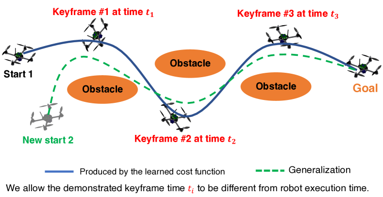
Figure 1: Illustration of learning from sparsely demonstrated keyframes. Each keyframe is a desired output with a time stamp. We aim to learn an objective function from keyframes such that the robot motion (blue line) follows these keyframes. At first glance, it may seem a problem of ‘curve fitting’ (i.e., finding a kinematic path). However, a key difference of our problem is that learning an objective function enables a robot to generalize new motion in unseen situations, such as given a new initial condition (green dashed line). A key feature of the proposed method is that in addition to learning an objective function, we jointly learn a time-warping function to account for the misalignment between the keyframe time $t_{i}$ and robot actual execution time (due to dynamics constraint).

LfD can be broadly categorized into two classes based on what to learn from demonstrations. The first branch of LfD focuses on learning policies [5, 6, 7, 8, 9], which maps directly from robot states, environment, or raw observation data to robot actions. While effective in many situations, policy learning typically requires a considerable amount of demonstration data, and the learned policy may generalize poorly to unseen tasks [1]. To alleviate this, the second line of LfD focuses on learning an objective (cost or reward) function from demonstrations [10], from which the policies or trajectories are derived. These methods assume the optimality of demonstrations and use inverse reinforcement learning (IRL) [11] or inverse optimal control (IOC) [12] to estimate objective functions. Since an objective function is a compact and high-level representation of a task and control principle, learning objective functions has shown an advantage over policy imitation in terms of better generalization [13] and relatively lower data complexity [10]. Despite appealing, objective learning based LfD inherits some limitations from existing IOC/IRL methods [14, 15, 16, 17, 18, 19].

First, existing IOC/IRL methods cannot handle the time misalignment between demonstrations and actual execution of a robot [20]. For instance, the speed of demonstrations maybe not be achievable by a robot, as the robot is actuated by weak motors and cannot move as fast as the demonstrations. Second, existing methods usually require the demonstrations of complete motion trajectories or at least a continuous segment of states-inputs, making it challenging in data collection for high-dimensional and long-horizon tasks. Third, existing IOC/IRL may not be efficient when handling high-dimensional continuous systems/tasks or learning complex objective functions, such as deep neural network objective functions.

This paper develops the Continuous Pontryagin Differentiable Programming method, abbreviated as the Continuous PDP, to address the existing challenges. The method requires only a few keyframes demonstrated at sparse time instances, and it learns both an objective function and a time-warping function, which accounts for the time misalignment between demonstration and robot actual execution. The Continuous PDP minimizes a discrepancy loss between the robot reproduced motion and the given keyframes via the projected gradient descent. This is done by efficiently computing the analytical gradient of the robot trajectory with respect to tunable parameters in the objective and time-warping functions. The highlights of the Continuous PDP are listed as follows.

• It requires as input the keyframe demonstrations, defined as a small number of sparse desired task-space outputs, which the robot is expected to follow sequentially, as in Fig. 1.

• As the time stamp of each keyframe may not correctly reflect the time of robot execution, in addition to learning an objective function, the method jointly searches for a time-warping function, which accounts for the time misalignment between keyframes and robot execution.

• The method can efficiently handle continuous-time high-dimensional systems and accepts any differentiable parameterization of objective functions.

I-A Related Work

Since the theme of this paper belongs to the category of objective learning, in the following we mainly review IOC/IRL methods. For other types of LfD, e.g., learning policies, please refer to the recent surveys [1, 21].

I-A1 Classic Strategies in IOC/IRL

Existing IOC/IRL methods can be categorized into two classes. The first class adopts a bi-level framework, where an objective function is updated on an outer level while the corresponding reinforcement learning (or optimal control) problem is solved on an inner level. Different methods in this class use different strategies to update an objective function. Representative work includes feature-matching IRL [10], where an objective function is updated to match the feature values of the reproduced trajectory with the ones of the demonstrations, max-margin IRL [14, 22], where an objective function is updated by maximizing the margin between the objective value of the reproduced trajectory and that of demonstrations, and max-entropy IRL [15], which finds an objective function such that the trajectory distribution has maximum entropy while subject to the empirical feature values. The second class of IOC/IRL [17, 18, 19, 23, 24] directly solves for objective function parameters by establishing the optimality conditions, such as KKT conditions [25] or Pontryagin’s Maximum Principle [26, 27]. The key idea is that a demonstration is assumed to be optimal and thus must satisfy the optimality condition. By directly minimizing the violation of the optimality conditions by demonstration data, one can compute the objective function parameters.

I-A2 IOC with Trajectory Loss

One type of bi-level IOC/IRL formulation also uses a trajectory loss as its learning criterion. A trajectory loss is to evaluate the discrepancy between the demonstrations and the robot motion reproduced by the objective function estimate. For example, [16] and [28] develop a bi-level IOC approach which learns an objective function from human locomotion data. In their work, the trajectory loss is minimized via a derivative-free technique [29], where the key is to approximate the loss using a quadratic function. The approach requires solving optimal control problems multiple times at each update, thus is computationally expensive. Further, the derivative-free methods are known to be challenging for the problem of large size [30]. In [31], the authors convert a bi-level IOC to a plain optimization by replacing the lower-level optimal control problem with its optimality conditions (the Pontryagin’s Maximum Principle). Although the converted plain optimization can be solved by an off-the-shelf nonlinear optimization solver, the decision variables of the plain optimization include both objective parameters and system trajectory (and dual variables); thus dramatically increasing the size of the optimization. Besides, both lines of methods have not considered the time misalignment between demonstrations and robot execution.

Compared to the derivative-free methods in [16, 28], the proposed Continuous PDP solves IOC/IRL by directly computing the analytical gradient of a trajectory loss with respect to tunable parameters in an objective function and a time-warping function, thus is capable of solving high-dimensional continuous tasks. Compared to [31], the Continuous PDP maintains the bi-level hierarchy of the problem and solves IOC by differentiating through the inner-level optimal control system. Maintaining a bi-level structure enables us to treat the outer and inner level subproblems separately, avoiding the mixed treatment that can lead to a dramatic increase in the size of optimization. In Section V-E3, we provide the comparison between the Continuous PDP and [31].

I-A3 IOC/IRL via differentiable through inner-level optimization

The recent work focuses on solving bi-level IOC/IRL by differentiating through inner-level optimization. E.g., [32] learns a cost function from visual demonstrations by differentiating through the inner-level MPC. Specifically, those methods treat the inner-level optimization as an unrolling computational graph of repetitively applying gradient descent, such that the automatic differentiation [33] can be applied. However, as shown in [34] and [35], auto-differentiating an ‘unrolling’ graph has the following drawback: (i) it needs to store all intermediate results along with the graph, thus is memory-expensive; and (ii) the accuracy of the unrolling differentiation depends on the length of the ‘unrolled’ graph, thus facing a trade-off between complexity and accuracy. In contrast, the Continuous PDP computes the gradient directly on the optimal trajectory produced from the inner level, without memorizing how this inner-level solution is obtained. Thus, there are no above challenges for the proposed method.

I-A4 Time-warping

Using time-warping functions to model the time misalignment between two temporal sequences has been extensively studied in signal processing [36] and pattern recognition [37]. In [38, 39], time-warping is used in LfD for learning and producing robot trajectories. In [20], a time-warping function between robot and demonstrator is learned for optimal tracking. All the above methods focus on learning policy or trajectory models instead of objective functions. For time-misalignment in IOC/IRL, a main technical challenge is how to incorporate the search of a time-warping function into the objective learning process. The Continuous PDP addresses this challenge by finding an objective function and a time-warping function simultaneously using gradient descent.

I-A5 Incomplete Trajectory or Sparse Waypoints

Some methods focus on learning from incomplete trajectories. In [23, 40], the authors develop a method to solve IOC with trajectory segments. It requires the length of a segment to satisfy a recovery condition and cannot directly learn from sparse points. [41, 42] consider learning from a set of sparse waypoints, but they learn a kinematic model instead of an objective function. Compared to those methods, the proposed method learns an objective function and a time-warping function from a small set of time-stamped sparse keyframes, i.e., a few desired task-space outputs. In Section V-E1, we will provide a comparison with [41].

I-A6 Sensitivity Analysis and Continuous PDP

The idea of the Continuous PDP is similar to the well-known sensitivity analysis [43, 44] in nonlinear optimization, where the KKT conditions are differentiated to obtain the gradient of a solution with respect to the objective function parameters. In sensitivity analysis, it requires to compute the inverse of the Hessian matrix in order to apply the well-known implicit function theorem [45]. If trying to apply the sensitivity analysis to a continuous-time optimal control problem in our formulation, we may face the following challenge. Since the optimality condition of a continuous-time optimal control problem is Pontryagin’s Maximum Principle [26], which is a set of ODE equations. To apply the sensitivity analysis, one would need to first discretize the continuous-time system, and this will lead to a Hessian matrix of the size at least $\frac{T}{\Delta t}\times\frac{T}{\Delta t}$ ($T$ is the time horizon, and $\Delta t$ is the discretization interval); this will cause huge computation cost when taking its inverse (the complexity is at least $\mathcal{O}((\frac{T}{\Delta t})^{2})$). The reason why we do not formulate the problem in discrete-time in the first place is that otherwise, learning a discrete time-warping function will lead the problem to a mixed-integer optimization, which becomes more challenging to attack.

Compared to sensitivity analysis, the Continuous PDP has the following new technical aspects. First, it directly differentiates the ODE equations in Pontryagin’s Maximum Principle [26], producing Differential Pontryagin’s Maximum Principle; and second, importantly, it develops Riccati-type equations to solve the Differential Pontryagin’s Maximum Principle to obtain the trajectory gradient (Lemma 1). The complexity of this process is only $\mathcal{O}(T)$. The Continuous PDP is an extension of our previous work Pontryagin Differentiable Programming (PDP) [34, 46] into the continuous-time systems. For a more detailed comparison between PDP and the sensitivity analysis, we refer the reader to [34, 46].

The following paper is organized as follows: Section II sets up the problem. Section III reformulates the problem using time-warping techniques. Section IV proposes the Continuous PDP method. Experiments are given in Sections V and VI. Section VII presents discussion, and Section VIII draws conclusions.

II Problem Formulation

Consider a robot with the following continuous dynamics:

$$\boldsymbol{\dot{x}}(t)=\boldsymbol{f}(\boldsymbol{x}(t),\boldsymbol{u}(t))\quad\text{with}\quad\boldsymbol{x}(0),$$ (1)

where $\boldsymbol{x}(t)\in\mathbb{R}^{n}$ is the robot state; $\boldsymbol{u}(t)\in\mathbb{R}^{m}$ is the control input; vector function $\boldsymbol{f}:\mathbb{R}^{n}\times\mathbb{R}^{m}\mapsto\mathbb{R}^{n}$ is assumed to be twice-differentiable, and $t\in[0,\infty)$ is time. Suppose the robot motion over a time horizon $t_{f}>0$ is controlled by minimizing the following parameterized cost function:

$$J(\boldsymbol{p})=\int_{0}^{t_{f}}c(\boldsymbol{x}(t),\boldsymbol{u}(t),{\boldsymbol{p}})dt+h(\boldsymbol{x}(t_{f}),{\boldsymbol{p}}),$$ (2)

where $c(\boldsymbol{x},\boldsymbol{u},{\boldsymbol{p}})$ and $h{(\boldsymbol{x},\boldsymbol{p}})$ are the running and final costs, respectively, both of which are assumed twice-differentiable; and $\boldsymbol{p}\in\mathbb{R}^{r}$ is a tunable parameter vector. For a fixed choice of $\boldsymbol{p}$, the robot produces a trajectory of states and inputs

$$\boldsymbol{\xi}_{\boldsymbol{p}}=\{\boldsymbol{\xi}_{\boldsymbol{p}}(t)\,|\,0\leq t\leq t_{f}\}\,\,\text{with}\,\,\boldsymbol{\xi}_{\boldsymbol{p}}(t)=\{\boldsymbol{x}_{\boldsymbol{p}}(t),\boldsymbol{u}_{\boldsymbol{p}}(t)\}.$$ (3)

which minimizes (2) subject to (1). The subscript in $\boldsymbol{\xi}_{\boldsymbol{p}}$ means that the trajectory implicitly depends on $\boldsymbol{p}$.

The goal of learning from demonstrations is to estimate the cost function parameter $\boldsymbol{p}$ from the given demonstrations by a user (usually a human). Suppose that a user provides demonstrations in a task space (e.g., Cartesian space or vision measurement), which is a known differentiable mapping of the robot state-input pair:

$$\boldsymbol{y}=\boldsymbol{g}(\boldsymbol{x},\boldsymbol{u}),$$ (4)

where $\boldsymbol{g}:\mathbb{R}^{n}\times\mathbb{R}^{m}\rightarrow\mathbb{R}^{o}$ defines a mapping from the robot state-input to a task output $\boldsymbol{y}\in\mathbb{R}^{o}$. The user’s demonstrations include (i) an expected time horizon $T$, and (ii) a number of $N$ keyframes, each of which is a desired output labeled with an expected time stamp $\tau_{i}$, denoted as

$$\mathcal{D}=\{\boldsymbol{y}^{*}(\tau_{i})\,|\,\tau_{i}\in[0,T],\,i=1,2,\cdots,N\}.$$ (5)

Here, $\boldsymbol{y}^{*}(\tau_{i})$ is the $i$th keyframe demonstrated by the user, and ${\tau_{i}}$ is the expected time stamp at which the user wants the robot to reach $\boldsymbol{y}^{*}(\tau_{i})$. The keyframe time $\{\tau_{1},\tau_{2},...,\tau_{N}\}$ can be sparsely located within range $[0,T]$. As the user can freely choose $N$ and $\tau_{i}$ relative to the expected horizon $T$, we call $\mathcal{D}$ as keyframes. As shown later in experiments, $N$ can be small.

Note that both the expected horizon $T$ and the expected time stamps $\tau_{i}$ are in the time axis of the user’s demonstration. This demonstration time axis may not be identical to the actual time axis of robot execution; in other words, $T$ and $\tau_{i}$ may not be achievable by the robot. For example, when the robot is actuated by a weak servo motor, its motion inherently cannot meet $\tau_{i}$. To accommodate the time misalignment between the robot execution and keyframes, we introduce a time warping function:

$$t=w(\tau),$$ (6)

which maps from keyframe time $\tau$ to robot time $t$. We make the following reasonable assumption: $w$ is strictly increasing in the range $[0,T]$, continuously differentiable, and $w(0)=0$.

Given the keyframes $\mathcal{D}$, the problem of interest is to find cost function parameter $\boldsymbol{p}$ and a time-warping function $w(\cdot)$ such that the task discrepancy loss is minimized:

$$\min\limits_{\boldsymbol{p},w}\sum\nolimits_{i=1}^{N}l\Big{(}\boldsymbol{y}^{*}(\tau_{i}),\boldsymbol{g}\big{(}\boldsymbol{\xi}_{\boldsymbol{p}}(w(\tau_{i}))\big{)}\Big{)},$$ (7)

where ${l}(\boldsymbol{a},\boldsymbol{b})$ is a given differentiable scalar function defined in the task space which quantifies a distance metric between vectors $\boldsymbol{a}$ and $\boldsymbol{b}$, e.g., $l(\boldsymbol{a},\boldsymbol{b})=\lVert\boldsymbol{a}-\boldsymbol{b}\rVert^{2}$. Minimizing (7) means that we want the robot to find cost function parameter $\boldsymbol{p}$ and a time-warping function $w(\cdot)$, such that its reproduced trajectory gets as close to the given keyframes as possible.

III Problem Reformulation based on Time-Warping Techniques

In this section, we re-formulate the problem of interest using the time-warping techniques.

III-A Parametric Time Warping Function

To facilitate learning of an unknown time-warping function, we first parameterize the time-warping function. Recall that a differentiable time-warping function ${w}(\tau)$ satisfies $w(0)=0$ and is strictly increasing in the range $[0,T]$, i.e.,

$$v(\tau)=\frac{dw(\tau)}{d\tau}>0$$ (8)

for all $\tau\in[0,T]$. We use a polynomial time-warping function:

$$t=w_{\boldsymbol{\beta}}(\tau)=\sum\nolimits_{i=1}^{s}\beta_{i}\tau^{i},$$ (9)

where $\boldsymbol{\beta}=[\beta_{1},\beta_{2},\cdots,\beta_{s}]^{\mkern-1.5mu\mathsf{T}}\in\mathbb{R}^{s}$ is the coefficient vector. Since $w_{\boldsymbol{\beta}}(0)=0$, there is no constant (zero-order) term in (9) (i.e., $\beta_{0}=0$). Due to the requirement of ${dw_{\boldsymbol{\beta}}}/{d\tau}=v_{\boldsymbol{\beta}}(\tau)>0$ for all $\tau\in[0,T]$, one can obtain a feasible set, denoted as $\Omega_{\boldsymbol{\beta}}$, such that $\frac{dw_{\boldsymbol{\beta}}(\tau)}{d\tau}>0$ for all $\tau\in[0,T]$ if $\boldsymbol{\beta}\in\Omega_{\boldsymbol{\beta}}$. The choice of polynomial degree $s$ will decide the representation power of (8): larger $s$ means that $w_{\boldsymbol{\beta}}(\tau)$ can represent more complex time warping curves. Note that although we use a polynomial time-warping function, the method in this paper allows for more general parameterization of a time-warping function, as long as it is differentiable. This paper uses polynomial time-warping functions due to the simplicity for implementation.

III-B Equivalent Formulation by Time Warping

Substituting the parametric time-warping function ${w}_{\boldsymbol{\beta}}$ in (9) into both the robot dynamics (1) and cost function (2), we obtain the following time-warped dynamics

$$\frac{d\boldsymbol{x}}{d{\tau}}=\frac{d{w}_{\boldsymbol{\beta}}}{d\tau}\boldsymbol{f}\Big{(}\boldsymbol{x}(w_{\boldsymbol{\beta}}(\tau)),\boldsymbol{u}(w_{\boldsymbol{\beta}}(\tau))\Big{)}\quad\text{with}\,\,\boldsymbol{x}(0),$$ (10)

and the time-warped cost function

$$J(\boldsymbol{p},\boldsymbol{\beta})= \int_{0}^{T}\frac{dw_{\boldsymbol{\beta}}}{d\tau}c_{\boldsymbol{p}}(\boldsymbol{x}(w_{\boldsymbol{\beta}}(\tau)),\boldsymbol{u}(w_{\boldsymbol{\beta}}(\tau)))d\tau$$ (11)

$$+h_{\boldsymbol{p}}(\boldsymbol{x}(w_{\boldsymbol{\beta}}(T))).$$

Here, the left side of (10) is due to chain rule: $\frac{d\boldsymbol{x}}{d\tau}=\dot{\boldsymbol{x}}\frac{dt}{d\tau}$, and the time horizon satisfies $t_{f}=w_{\boldsymbol{\beta}}(T)$ (note that $T$ is specified by the demonstrator). For notation simplicity, we write $\frac{d{w}_{\boldsymbol{\beta}}}{d\tau}=v_{\boldsymbol{\beta}}(\tau)$, $\boldsymbol{x}(w(\tau))=\boldsymbol{x}(\tau)$, $\boldsymbol{u}(w(\tau))=\boldsymbol{u}(\tau)$, and $\frac{d\boldsymbol{x}}{d{\tau}}=\dot{\boldsymbol{x}}(\tau)$. Then, the above time-warped dynamics (10) and time-warped cost function (11) are rewritten as:

$$\dot{\boldsymbol{x}}(\tau)=v_{\boldsymbol{\beta}}(\tau)\boldsymbol{f}(\boldsymbol{x}(\tau),\boldsymbol{u}(\tau))\quad\text{with}\,\,\boldsymbol{x}(0)$$ (12a)

and

$$J(\boldsymbol{p},\boldsymbol{\beta}){=}\int_{0}^{T}v_{\boldsymbol{\beta}}(\tau)c(\boldsymbol{x}(\tau),\boldsymbol{u}(\tau),{\boldsymbol{p}})d\tau+h(\boldsymbol{x}(T),{\boldsymbol{p}}),$$ (12b)

respectively. We pack the tunable cost parameter $\boldsymbol{p}$ and time-warping parameter $\boldsymbol{\beta}$ together as

$$\boldsymbol{{\theta}}=[\boldsymbol{p}^{\mkern-1.5mu\mathsf{T}},\boldsymbol{\beta}^{\mkern-1.5mu\mathsf{T}}]^{\mkern-1.5mu\mathsf{T}}\in\mathbb{R}^{r+s}.$$ (13)

For a fixed $\boldsymbol{{\theta}}$, the optimal trajectory from solving the above time-warped optimal control system (12) is rewritten as

$$\boldsymbol{\xi}_{\boldsymbol{\theta}}=\{\boldsymbol{\xi}_{\boldsymbol{\theta}}(\tau)\,\,|\,\,0\leq\tau\leq T\},\,\,$$ (14)

with $\boldsymbol{\xi}_{\boldsymbol{\theta}}(\tau)=\{\boldsymbol{x}_{\boldsymbol{\theta}}(\tau),\boldsymbol{u}_{\boldsymbol{\theta}}(\tau)\}$. The discrepancy loss (7) can now be defined as

$$L(\boldsymbol{\xi}_{\boldsymbol{\theta}},\mathcal{D})=\sum_{i=1}^{N}l\Big{(}\boldsymbol{y}^{*}(\tau_{i}),\,\,\boldsymbol{g}\big{(}\boldsymbol{\xi}_{\boldsymbol{\theta}}(\tau_{i})\big{)}\Big{)}.$$ (15)

Minimizing (15) over $\boldsymbol{\theta}$ is a process of simultaneously searching for a cost function $J(\boldsymbol{p})$ and time-warping function $w_{\boldsymbol{\beta}}(\tau)$. In sum, the problem of interest is now reformulated as the following optimization

$$\min_{\boldsymbol{\theta}\in\boldsymbol{\Theta}}\,\,\,L(\boldsymbol{\xi}_{\boldsymbol{\theta}},\mathcal{D})$$ (16)

$$\quad\text{s.t.}\quad\boldsymbol{\xi}_{\boldsymbol{\theta}}\text{ is from the optimal control system (\ref{ocsys})}.$$

Here $\boldsymbol{\Theta}$ defines a feasible set of $\boldsymbol{\theta}$, $\boldsymbol{\Theta}=\mathbb{R}^{r}\times\Omega_{\boldsymbol{\beta}}$. (16) is a bi-level optimization, where the upper level is to minimize a discrepancy loss between the keyframes $\mathcal{D}$ and the reproduced time-warped trajectory $\boldsymbol{\xi}_{\boldsymbol{\theta}}$, and the inner level is to generate such $\boldsymbol{\xi}_{\boldsymbol{\theta}}$ by solving the optimal control problem (12). In the next section, we will develop the Continuous Pontryagin Differentiable Programming to efficiently solve (16).

IV Continuous Pontryagin Differentiable Programming

IV-A Algorithm Overview

To solve the optimization (16), we start with an arbitrary initial guess $\boldsymbol{\theta}_{0}\in\boldsymbol{\Theta}$, and apply the gradient descent

$$\boldsymbol{\theta}_{k+1}=\operatorname{Proj}_{\boldsymbol{\Theta}}\left(\boldsymbol{\theta}_{k}-\eta_{k}\frac{dL}{d\boldsymbol{\theta}}\Bigr{|}_{\boldsymbol{\theta}_{k}}\right),$$ (17)

where $k$ is the iteration index; $\eta_{k}$ is the step size (or learning rate); $\operatorname{Proj}_{\boldsymbol{\Theta}}$ is a projection operator to enforce the feasibility of $\boldsymbol{\theta}_{k}$ in $\boldsymbol{\Theta}$, e.g., $\operatorname{Proj}_{\boldsymbol{\Theta}}(\boldsymbol{\theta})=\arg\min_{\boldsymbol{z}\in\boldsymbol{\Theta}}\lVert\boldsymbol{\theta}-\boldsymbol{z}\rVert$; and $\frac{dL}{d\boldsymbol{\theta}}\bigr{|}_{\boldsymbol{\theta}_{k}}$ denotes the gradient of the loss (15) directly with respect to $\boldsymbol{\theta}$ evaluated at $\boldsymbol{\theta}_{k}$. Applying the chain rule, we have

$$\frac{dL}{d\boldsymbol{\theta}}\Bigr{|}_{\boldsymbol{\theta}_{k}}=\sum_{i=1}^{N}\frac{\partial l}{\partial\boldsymbol{\xi}_{\boldsymbol{\theta}}(\tau_{i})}\Bigr{|}_{\boldsymbol{\xi}_{\boldsymbol{\theta}_{k}}(\tau_{i})}\frac{{\partial\boldsymbol{\xi}_{\boldsymbol{\theta}}{(\tau_{i})}}}{\partial\boldsymbol{\theta}}\Big{\rvert}_{{\boldsymbol{\theta}}_{k}},$$ (18)

where $\frac{\partial l}{\partial\boldsymbol{\xi}_{\boldsymbol{\theta}}{(\tau_{i})}}\big{\rvert}_{\boldsymbol{\xi}_{\boldsymbol{\theta}_{k}}(\tau_{i})}$ is the gradient of the single keyframe loss $l=\Big{(}\boldsymbol{y}^{*}(\tau_{i}),\,\,\boldsymbol{g}\big{(}\boldsymbol{\xi}_{\boldsymbol{\theta}}(\tau_{i})\big{)}\Big{)}$ in (15) with respect to the time-$\tau_{i}$ trajectory point $\boldsymbol{\xi}_{\boldsymbol{\theta}}{(\tau_{i})}$, evaluated at value $\boldsymbol{\xi}_{\boldsymbol{\theta}_{k}}{(\tau_{i})}$, and $\frac{{\partial\boldsymbol{\xi}_{\boldsymbol{\theta}}{(\tau_{i})}}}{\partial\boldsymbol{\theta}}\big{\rvert}_{{\boldsymbol{\theta}}_{k}}$ is the gradient of the time-$\tau_{i}$ trajectory point $\boldsymbol{\xi}_{\boldsymbol{\theta}}{(\tau_{i})}$, with respect to $\boldsymbol{\theta}$, evaluated at value $\boldsymbol{\theta}_{k}$. From (17) and (18), we can draw the computational diagram in Fig. 2. Fig. 2 shows that at each iteration $k$, the update of $\boldsymbol{\theta}_{k}$ includes the following three steps:

• Obtain the optimal trajectory $\boldsymbol{{\xi}}_{\boldsymbol{\theta}_{k}}$ by solving the optimal control (trajectory optimization) problem (12) with current $\boldsymbol{\theta}_{k}$;

• Compute the gradient $\frac{\partial l}{\partial\boldsymbol{\xi}_{\boldsymbol{\theta}}{(\tau_{i})}}\big{\rvert}_{\boldsymbol{\xi}_{\boldsymbol{\theta}_{k}}(\tau_{i})}$;

• Compute the gradient $\frac{{\partial\boldsymbol{\xi}_{\boldsymbol{\theta}}{(\tau_{i})}}}{\partial\boldsymbol{\theta}}\big{\rvert}_{{\boldsymbol{\theta}}_{k}}$;

• Apply chain rule (18) to compute $\frac{dL}{d\boldsymbol{\theta}}\big{\rvert}_{\boldsymbol{\theta}_{k}}$, and update $\boldsymbol{\theta}_{k}$ using (17) to $\boldsymbol{\theta}_{k+1}$.

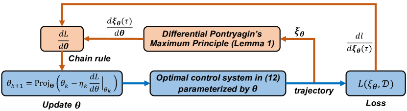
Figure 2: Computational diagram of the Continuous Pontryagin Differentiable Programming.

The interpretation of the above procedure is straightforward. At each update $k$, the first step is to use the current parameter $\boldsymbol{\theta}_{k}$ to compute the current optimal trajectory $\boldsymbol{\xi}_{\boldsymbol{\theta}_{k}}$ by solving the optimal control problem (12). In Step 2 and Step 3, the gradient of the loss with respect to the trajectory point, $\frac{\partial l}{\partial\boldsymbol{\xi}_{\boldsymbol{\theta}}{(\tau_{i})}}\big{\rvert}_{\boldsymbol{\xi}_{\boldsymbol{\theta}_{k}}(\tau_{i})}$, and the gradient of the trajectory point with respect to parameters, $\frac{{\partial\boldsymbol{\xi}_{\boldsymbol{\theta}}{(\tau_{i})}}}{\partial\boldsymbol{\theta}}\big{\rvert}_{{\boldsymbol{\theta}}_{k}}$, are computed, respectively. In Step 4, the total gradient of the loss with respect to the parameter, $\frac{dL}{d\boldsymbol{\theta}}\big{\rvert}_{\boldsymbol{\theta}_{k}}$, is assembled via chain rule (18), and then used to update ${\boldsymbol{\theta}_{k}}$ by the projected gradient descent (17).

In Step 1, the optimal trajectory $\boldsymbol{\xi}_{\boldsymbol{\theta}_{k}}$ can be solved by available optimal control (trajectory optimization) solvers such as iLQR [47], DDP [48], Casadi [49], GPOPS [50], etc. In Step 2, the gradient $\frac{\partial L}{\partial\boldsymbol{\xi}_{\boldsymbol{\theta}}{(\tau_{i})}}$ can be readily computed by directly differentiating the given loss (15). The main challenge, however, lies in Step 3, i.e., computing $\frac{{\partial\boldsymbol{\xi}_{\boldsymbol{\theta}}}}{\partial\boldsymbol{\theta}}\big{\rvert}_{{\boldsymbol{\theta}}_{k}}$, the gradient of the optimal trajectory $\boldsymbol{\xi}_{\boldsymbol{\theta}}$ with respect to the parameter $\boldsymbol{\theta}$ of the optimal control system (12). In what follows, we will efficiently solve it by proposing the technique of Differential Pontryagin’s Maximum Principle. For notation simplicity, we suppress the iteration index $k$ below.

IV-B Differential Pontryagin’s Maximum Principle

In this section, we focus on efficiently solving the analytical gradient of a trajectory of a continuous-time optimal control system with respect to the system parameter. We assume that the resulting optimal trajectory $\boldsymbol{\xi}_{\boldsymbol{\theta}}$ in (14) is differentiable with respect to the system parameter $\boldsymbol{\theta}$. This assumption is satisfied if $\boldsymbol{\xi}_{\boldsymbol{\theta}}$ satisfies the second-order sufficient condition, that is, $\boldsymbol{\theta}$ is a locally unique optimal trajectory (see Lemma 1 in [46]). Both our later experiments and previous empirical results [34, 51] show that the differentiability condition is very mild. For more detailed results about the differentiability for a general optimal control system with respect to system parameters, we refer the reader to [46].

Consider an optimal trajectory $\boldsymbol{\xi}_{\boldsymbol{\theta}}$ in (14) produced by an optimal control system (12) with a fixed $\boldsymbol{\theta}$. The Pontryagin’s Maximum Principle [26] states a set of ODE conditions that $\boldsymbol{\xi}_{\boldsymbol{\theta}}$ must satisfy. To present the Pontryagin’s Maximum Principle, define the Hamiltonian [52]:

$$H(\tau)=v_{\boldsymbol{\beta}}(\tau)c_{\boldsymbol{p}}(\boldsymbol{x}(\tau),\boldsymbol{u}(\tau))\\ +\boldsymbol{\lambda}(\tau)^{\mkern-1.5mu\mathsf{T}}v_{\boldsymbol{\beta}}(\tau)\boldsymbol{f}(\boldsymbol{x}(\tau),\boldsymbol{u}(\tau)),$$ (19)

where $\boldsymbol{\lambda}(\tau)\in\mathbb{R}^{n}$ is called the costate, $0\leq\tau\leq T$. According to the Pontryagin’s Maximum Principle [26], there exists

$$\{\boldsymbol{\lambda}_{\boldsymbol{\theta}}(\tau)\,|\,0\leq\tau\leq T\},$$ (20)

associated with the optimal trajectory $\boldsymbol{\xi}_{\boldsymbol{\theta}}$ in (14), such that the following ODE equations hold [26]:

$$\dot{\boldsymbol{x}}_{\boldsymbol{\theta}}(\tau) =\frac{\partial H}{\partial\boldsymbol{\lambda}_{\boldsymbol{\theta}}}(\boldsymbol{x}_{\boldsymbol{\theta}}(\tau),\boldsymbol{u}_{\boldsymbol{\theta}}(\tau),\boldsymbol{\lambda}_{\boldsymbol{\theta}}(\tau)),$$ (21a)

$$-\dot{\boldsymbol{\lambda}}_{\boldsymbol{\theta}}(\tau) =\frac{\partial H}{\partial\boldsymbol{x}}(\boldsymbol{x}_{\boldsymbol{\theta}}(\tau),\boldsymbol{u}_{\boldsymbol{\theta}}(\tau),\boldsymbol{\lambda}_{\boldsymbol{\theta}}(\tau)),$$ (21b)

$$\boldsymbol{0} =\frac{\partial H}{\partial\boldsymbol{u}}(\boldsymbol{x}_{\boldsymbol{\theta}}(\tau),\boldsymbol{u}_{\boldsymbol{\theta}}(\tau),\boldsymbol{\lambda}_{\boldsymbol{\theta}}(\tau)),$$ (21c)

$$\boldsymbol{\lambda}_{\boldsymbol{{\theta}}}(T) =\frac{\partial h_{\boldsymbol{p}}}{\partial\boldsymbol{x}}(\boldsymbol{x}_{\boldsymbol{\theta}}(T))\quad\text{and}\quad\boldsymbol{x}_{\boldsymbol{\theta}}(0)=\boldsymbol{x}(0).$$ (21d)

Here, (21a) is the dynamics; (21b) is the costate ODE; (21c) is the input ODE, and (21d) is the boundary conditions. Given $\boldsymbol{\xi}_{\boldsymbol{{\theta}}}$, one can always solve the corresponding $\{\boldsymbol{\lambda}_{\boldsymbol{\theta}}(\tau)\,|\,0\leq\tau\leq T\}$ by integrating the costate ODE in (21b) backward in time with the boundary condition in (21d).

Recall that our technical challenge is to obtain the gradient $\frac{{\partial\boldsymbol{\xi}_{\boldsymbol{\theta}}}}{\partial\boldsymbol{\theta}}$. Towards this goal, we differentiate the above Pontryagin’s Maximum Principle in (21) on both sides with respect to the system parameter $\boldsymbol{\theta}$, yielding the following Differential Pontryagin’s Maximum Principle:

$$\frac{d}{d\tau}(\frac{\partial\boldsymbol{x}_{\boldsymbol{\theta}}}{\partial\boldsymbol{\theta}}) =F(\tau)\frac{\partial\boldsymbol{x}_{\boldsymbol{\theta}}}{\partial\boldsymbol{\theta}}+G(\tau)\frac{\partial\boldsymbol{u}_{\boldsymbol{\theta}}}{\partial\boldsymbol{\theta}}+E(\tau),$$ (22a)

$${-}\frac{d}{d\tau}(\frac{\partial\boldsymbol{\lambda}_{\boldsymbol{\theta}}}{\partial\boldsymbol{\theta}}) =H_{xx}(\tau)\frac{\partial\boldsymbol{x}_{\boldsymbol{\theta}}}{\partial\boldsymbol{\theta}}+H_{xu}(\tau)\frac{\partial\boldsymbol{u}_{\boldsymbol{\theta}}}{\partial\boldsymbol{\theta}}$$

$$\qquad\qquad\qquad+{F}(\tau)^{\mkern-1.5mu\mathsf{T}}\frac{\partial\boldsymbol{\lambda}_{\boldsymbol{\theta}}}{\partial\boldsymbol{\theta}}+H_{xe}(\tau),$$ (22b)

$$\boldsymbol{0} =H_{ux}(\tau)\frac{\partial\boldsymbol{x}_{\boldsymbol{\theta}}}{\partial\boldsymbol{\theta}}+H_{uu}(\tau)\frac{\partial\boldsymbol{u}_{\boldsymbol{\theta}}}{\partial\boldsymbol{\theta}}$$

$$\qquad\qquad\qquad+{G}(\tau)^{\mkern-1.5mu\mathsf{T}}\frac{\partial\boldsymbol{\lambda}_{\boldsymbol{\theta}}}{\partial\boldsymbol{\theta}}+H_{ue}(\tau),$$ (22c)

$$\frac{\partial\boldsymbol{\lambda}_{\boldsymbol{\theta}}}{\partial\boldsymbol{\theta}}(T) =H_{xx}(T)\frac{\partial\boldsymbol{x}_{\boldsymbol{\theta}}}{\partial\boldsymbol{\theta}}+H_{xe}(T)$$

$$\qquad\qquad\qquad\quad\text{and}\quad\frac{\partial\boldsymbol{x}_{\boldsymbol{\theta}}}{\partial\boldsymbol{\theta}}(0)=\boldsymbol{0}.$$ (22d)

The coefficient matrices in the above (22) are defined as

$$F(\tau){=}\dfrac{\partial^{2}{H}}{\partial\boldsymbol{\lambda}_{\boldsymbol{\theta}}\partial\boldsymbol{{x}}_{\boldsymbol{\theta}}},\quad G(\tau){=}\dfrac{\partial^{2}{H}}{\partial\boldsymbol{\lambda}_{\boldsymbol{\theta}}\partial\boldsymbol{{u}}_{\boldsymbol{\theta}}},\quad E(\tau){=}\dfrac{\partial^{2}{H}}{\partial\boldsymbol{\lambda}_{\boldsymbol{\theta}}\partial\boldsymbol{\theta}},$$ (23a)

$$H_{xx}(\tau){=}\frac{\partial^{2}H}{(\partial\boldsymbol{{x}}_{\boldsymbol{\theta}})^{2}},\,\,H_{xu}(\tau){=}\frac{\partial^{2}H}{\partial\boldsymbol{{x}}_{\boldsymbol{\theta}}\partial\boldsymbol{{u}}_{\boldsymbol{\theta}}},\,H_{xe}(\tau){=}\frac{\partial^{2}H}{\partial\boldsymbol{{x}}_{\boldsymbol{\theta}}\partial\boldsymbol{\theta}},$$ (23b)

$$H_{ux}(\tau){=}H_{xu}^{\mkern-1.5mu\mathsf{T}}(\tau),\,\,\,\,H_{uu}(\tau){=}\dfrac{\partial^{2}H}{(\partial\boldsymbol{{u}}_{\boldsymbol{\theta}})^{2}},\quad H_{ue}(\tau){=}\dfrac{\partial^{2}H}{\partial\boldsymbol{{u}}_{\boldsymbol{\theta}}\partial\boldsymbol{\theta}},$$ (23c)

$$H_{xx}(T){=}\dfrac{\partial^{2}h_{\boldsymbol{p}}}{(\partial\boldsymbol{{x}}_{\boldsymbol{\theta}})^{2}},\,\,H_{xe}(T){=}\dfrac{\partial^{2}h_{\boldsymbol{p}}}{\partial\boldsymbol{{x}}_{\boldsymbol{\theta}}\partial\boldsymbol{\theta}}.$$ (23d)

Once we obtain the optimal trajectory $\boldsymbol{\xi}_{\boldsymbol{\theta}}$ and the associated costate trajectory $\{\boldsymbol{\lambda}_{\boldsymbol{\theta}}(\tau)\,|\,0\leq\tau\leq T\}$ in (20), all the above coefficient matrices in (23) are known and their computation is straightforward. Given the Differential Pontryagin’s Maximum Principle in (22), one can observe that these ODEs have a similar form to the original Pontryagin’s Maximum Principle in (21). Thus, if one thinks of $\frac{{\partial\boldsymbol{x}_{\boldsymbol{\theta}}}}{\partial\boldsymbol{\theta}}$ as a new state variable, $\frac{{\partial\boldsymbol{u}_{\boldsymbol{\theta}}}}{\partial\boldsymbol{\theta}}$ as a new control variable, and $\frac{{\partial\boldsymbol{\lambda}_{\boldsymbol{\theta}}}}{\partial\boldsymbol{\theta}}$ as a new costate variable, then the Differential Pontryagin’s Maximum Principle in (22) can be thought of as the Pontryagin’s Maximum Principle of a new LQR system, as investigated in [34, 46]. By deriving the equivalent Raccati-type equations, the lemma below gives an efficient way to compute the trajectory gradient $\frac{{\partial\boldsymbol{\xi}_{\boldsymbol{\theta}}(\tau)}}{\partial\boldsymbol{\theta}}$, $0\leq\tau\leq T$, from the above (22).

Lemma 1.

If ${H_{uu}(\tau)}$ in (23c) is invertible for all $0\leq\tau\leq T$, define the following differential equations for matrix variables $P(\tau)\in\mathbb{R}^{n\times n}$ and $W(\tau)\in\mathbb{R}^{n\times{(r+s)}}$:

$$-{\dot{{P}}} ={{Q}}(\tau)+{{A}}(\tau)^{\mkern-1.5mu\mathsf{T}}{{P}}+{{P}}{{A}}(\tau)-{{P}}{{R}}(\tau){{P}},$$ (24a)

$${\dot{{W}}} ={{P}}{{R}}(\tau){{W}}-{{A}}(\tau)^{\mkern-1.5mu\mathsf{T}}{{W}}-{{P}}{{M}}(\tau)-{{N}}(\tau),$$ (24b)

with ${{P}}(T)=H_{xx}(T)$ and ${{W}}(T)=H_{xe}(T).$ Here,

$${{A}}(\tau) =F-G(H_{uu})^{-1}H_{ux},$$ (25a)

$${{R}}(\tau) =G(H_{uu})^{-1}G^{\mkern-1.5mu\mathsf{T}},$$ (25b)

$${{M}}(\tau) =E-G(H_{uu})^{-1}H_{ue},$$ (25c)

$${{Q}}(\tau) =H_{xx}-H_{xu}(H_{uu})^{-1}H_{ux},$$ (25d)

$${{N}}(\tau) =H_{xe}-H_{xu}(H_{uu})^{-1}H_{ue},$$ (25e)

are all known given (23). The gradient of the optimal trajectory $\boldsymbol{\xi}_{\boldsymbol{\theta}}$, denoted as

$$\small\frac{{\partial\boldsymbol{\xi}_{\boldsymbol{\theta}}(\tau)}}{\partial\boldsymbol{\theta}}=\left(\frac{{\partial\boldsymbol{x}_{\boldsymbol{\theta}}}}{\partial\boldsymbol{\theta}}(\tau),\frac{{\partial\boldsymbol{u}_{\boldsymbol{\theta}}}}{\partial\boldsymbol{\theta}}(\tau)\right),\quad 0\leq\tau\leq T$$ (26)

is obtained by integrating the following ODEs up to $\tau$:

$${\frac{{\partial\boldsymbol{u}_{\boldsymbol{\theta}}}}{\partial\boldsymbol{\theta}}} {=}-(H_{uu}(\tau))^{-1}\Big{(}H_{ux}(\tau)\frac{\partial\boldsymbol{x}_{\boldsymbol{\theta}}}{\partial\boldsymbol{\theta}}(\tau)+H_{ue}(\tau)$$

$$+{G(\tau)}^{\mkern-1.5mu\mathsf{T}}{{W}(\tau)}+{G(\tau)}^{\mkern-1.5mu\mathsf{T}}{{P}}(\tau)\frac{{\partial\boldsymbol{x}_{\boldsymbol{\theta}}}}{\partial\boldsymbol{\theta}}(\tau)\Big{)},$$ (27a)

$$\frac{d}{d\tau}\left({\frac{{\partial\boldsymbol{x}_{\boldsymbol{\theta}}}}{\partial\boldsymbol{\theta}}}\right) {=}F(\tau)\frac{{\partial\boldsymbol{x}_{\boldsymbol{\theta}}}}{\partial\boldsymbol{\theta}}(\tau)+G(\tau)\frac{{\partial\boldsymbol{u}_{\boldsymbol{\theta}}}}{\partial\boldsymbol{\theta}}(\tau)+E(\tau),$$ (27b)

with $\frac{\partial\boldsymbol{x}_{\boldsymbol{\theta}}}{\partial\boldsymbol{\theta}}{(0)}=\boldsymbol{0}$ in (22d). Here, the matrices $P(\tau)$ and $W(\tau)$ are solutions to (24a) and (24b), respectively.

The proof of Lemma 1 is given in Appendix. Lemma 1 states that for the optimal control system (12), the gradient of its optimal trajectory $\boldsymbol{\xi}_{\boldsymbol{\theta}}$ with respect to the system parameter $\boldsymbol{\theta}$ can be obtained in two steps: first, integrate (24) backward in time to obtain $P(\tau)$ and $W(\tau)$ for $0\leq\tau\leq T$; and second, obtain $\frac{{\partial\boldsymbol{\xi}_{\boldsymbol{\theta}}}}{\partial\boldsymbol{\theta}}({\tau})$ by integrating (27) forward in time. Based on the Differential Pontryagin’s Maximum Principle, Lemma 1 gives an efficient way to compute the gradient of an optimal trajectory with respect to the parameter in an optimal control system. By Lemma 1, one can obtain the derivative of the trajectory point $\boldsymbol{\xi}_{\boldsymbol{\theta}}(\tau)$, at any time $0\leq\tau\leq T$, with respect to the system parameter $\boldsymbol{\theta}$, i.e., $\frac{{\partial\boldsymbol{\xi}_{\boldsymbol{\theta}}}}{\partial\boldsymbol{\theta}}(\tau)$.

Additionally, we have the following comments on Lemma 1. First, (24) are Riccati-type equations, which are derived from Differential Pontryagin’s Maximum Principle in (22). Second, Lemma 1 requires the matrix $H_{uu}(\tau){=}\small\frac{\partial^{2}H}{\partial\boldsymbol{{u}}_{\boldsymbol{\theta}}\partial\boldsymbol{{u}}_{\boldsymbol{\theta}}}$ in (23c) to be invertible, this is in fact a necessary condition [46] for the differentiability of $\boldsymbol{\xi}_{\boldsymbol{\theta}}$. As we have mentioned at the beginning of this subsection, if $\boldsymbol{\xi}_{\boldsymbol{\theta}}$ satisfies the second-order sufficient condition (i.e., is a locally unique optimal trajectory) for the optimal control problem (12), then $\boldsymbol{\xi}_{\boldsymbol{\theta}}$ is differentiable in $\boldsymbol{\theta}$ and $H_{uu}(\tau)$ is automatically invertible (see [46] for the details and proofs). A similar invertiblility requirement is common in sensitivity analysis methods [43, 44], where they analogously requires the Hessian matrix to be invertible in order to apply the implicit function theorem [45]. Both our later experiments and other related existing work [34, 46, 35] have empirically shown that the invertibility of $H_{uu}(\tau)$ is a mild condition and could be easily satisfied. With Lemma 1, we summarize the overall algorithm of the Continuous PDP in Algorithm 1.

Input: keyframes $\mathcal{D}$ in (5) and learning rate $\{\eta_{k}\}$.

Initialization: initial parameter guess $\boldsymbol{\theta}_{0}$,

for $k=0,1,2,\cdots$ do

      

      Obtain the optimal trajectory $\boldsymbol{{\xi}}_{\boldsymbol{\theta}_{k}}$ by solving the optimal control problem in (12) with current $\boldsymbol{\theta}_{k}$;

      

      Obtain the costate trajectory $\{\boldsymbol{\lambda}_{\boldsymbol{\theta}_{k}}(\tau)\}$ by integrating (21b) given (21d);

      

      

      Compute $\frac{{\partial\boldsymbol{\xi}_{\boldsymbol{\theta}}{(\tau_{i})}}}{\partial\boldsymbol{\theta}}\big{\rvert}_{{\boldsymbol{\theta}}_{k}}$ using Lemma 1 for $i=1,2,\cdots N$;

      

      Compute $\frac{\partial l}{\partial\boldsymbol{\xi}_{\boldsymbol{\theta}}{(\tau_{i})}}\big{\rvert}_{\boldsymbol{\xi}_{\boldsymbol{\theta}_{k}}(\tau_{i})}$ from (15);

      

      Obtain $\frac{dL}{d\boldsymbol{\theta}}\rvert_{\boldsymbol{\theta}_{k}}$ using the chain rule (18);

      

      Update $\boldsymbol{\theta}_{k+1}\leftarrow\operatorname{Proj}_{\boldsymbol{\Theta}}\left(\boldsymbol{\theta}_{k}-\eta_{k}\frac{dL}{d\boldsymbol{\theta}}\bigr{|}_{\boldsymbol{\theta}_{k}}\right)$;

      

end for

Algorithm 1 Learning from sparse demonstrations.

V Numerical Experiments

In this section, we evaluate different aspects of the proposed method using a two-link robot arm performing reaching tasks. The dynamics of a robot arm (moving horizontally) is [53]

$$M(\boldsymbol{q})\ddot{\boldsymbol{q}}+c(\boldsymbol{q},\boldsymbol{\dot{q}})=\boldsymbol{\tau},$$ (28)

where $M(\boldsymbol{q})\in\mathbb{R}^{2\times 2}$ is the inertia matrix, $c(\boldsymbol{q},\boldsymbol{\dot{q}})\in\mathbb{R}^{2}$ is the Coriolis term; $\boldsymbol{q}=[q_{1},q_{2}]^{\mkern-1.5mu\mathsf{T}}\in\mathbb{R}^{2}$ is the joint angle vector, and $\boldsymbol{\tau}=[\tau_{1},\tau_{2}]^{\mkern-1.5mu\mathsf{T}}\in\mathbb{R}^{2}$ is the joint toque vector. The physical parameters for the dynamics are: $m_{1}{=}2\text{kg}$ and $m_{2}{=}1\text{kg}$ for the mass of each link; $l_{1}{=}1\text{m}$ and $l_{2}{=}1\text{m}$ for the length of each link (assume mass is evenly distributed). The state and control vectors are $\boldsymbol{x}=[\boldsymbol{q},\dot{\boldsymbol{q}}]^{\mkern-1.5mu\mathsf{T}}\in\mathbb{R}^{4}$ and $\boldsymbol{u}=\boldsymbol{\tau}\in\mathbb{R}^{2}$, respectively.

For the task of reaching to a goal state $\boldsymbol{x}^{\text{g}}=[q_{1}^{\text{g}},q_{2}^{\text{g}},0,0]^{\mkern-1.5mu\mathsf{T}}\in\mathbb{R}^{4}$, we set the cost function (2) as

$$c(\boldsymbol{x},\boldsymbol{u},\boldsymbol{p})= p_{1}(q_{1}-q_{1}^{\text{g}})^{2}+p_{2}(q_{2}-q_{2}^{\text{g}})^{2}+$$

$$p_{3}\,\dot{q}_{1}^{2}+p_{4}\,\dot{q}_{2}^{2}+0.5\lVert\boldsymbol{u}\rVert^{2},$$ (29a)

$$h(\boldsymbol{x},\boldsymbol{p})= p_{1}(q_{1}{-}q_{1}^{\text{g}})^{2}{+}p_{2}(q_{2}{-}q_{2}^{\text{g}})^{2}+p_{3}\,\dot{q}_{1}^{2}{+}p_{4}\,\dot{q}_{2}^{2}.$$ (29b)

with the tunable parameter $\boldsymbol{p}=[p_{1},p_{2},p_{3},p_{4}]^{\mkern-1.5mu\mathsf{T}}\in\mathbb{R}^{4}$. Note that (29) is a weighted distance-to-goal function with a fixed weight to $\lVert\boldsymbol{u}\rVert^{2}$, because otherwise, learning all weights will lead to scaling ambiguity [23]. We set the goal state $\boldsymbol{x}^{\text{g}}=[\frac{\pi}{2},0,0,0]^{\mkern-1.5mu\mathsf{T}}$, and the initial state $\boldsymbol{x}(0)=[-\frac{\pi}{2},\frac{3\pi}{4},-5,3]^{\mkern-1.5mu\mathsf{T}}$.

For parametric time-warping function (9), we simply use

$$t=w_{\boldsymbol{\beta}}(\tau)=\beta\tau,$$ (30)

with $\Omega_{\boldsymbol{\beta}}=\{\beta\,|\,\beta>0\}$ (more complex time-warping functions will be used later). The overall parameter to be tuned is $\boldsymbol{\theta}=[\boldsymbol{p}^{\mkern-1.5mu\mathsf{T}},\beta]^{\mkern-1.5mu\mathsf{T}}\in\mathbb{R}^{5}$. The task-space mapping (4) is

$$\boldsymbol{q}=\boldsymbol{g}(\boldsymbol{x},\boldsymbol{u}),$$ (31)

meaning that the keyframe only includes the position information. For the discrepancy loss (15), we use the squared $l_{2}$ norm:

$$L(\boldsymbol{\xi}_{\boldsymbol{\theta}},\mathcal{D})=\sum\nolimits_{i=1}^{N}\lVert\boldsymbol{q}^{*}(\tau_{i})-\boldsymbol{g}\big{(}\boldsymbol{\xi}_{\boldsymbol{\theta}}(\tau_{i})\big{)}\rVert^{2}.$$ (32)

In the following experiments, we evaluate different aspects of the method and provide analysis for each evaluation.

V-A Different Number of Keyframes

First, we evaluate the performance of the proposed method for learning from different numbers of keyframes. $\mathcal{D}$ is generated from known/true cost and time-warping functions. Given

$$\boldsymbol{\theta}^{\text{true}}=[3,3,3,3,5]^{\mkern-1.5mu\mathsf{T}},$$ (33)

the robot optimal trajectory is computed by solving the optimal control problem (12), shown in Fig. 3. Then, we select some points (red dots) from Fig. 3 as our keyframes $\mathcal{D}$, listed in Table I. We evaluate the performance of the proposed method to recover $\boldsymbol{\theta}^{\text{true}}$ given different numbers of the keyframes. The learning rate is $\eta=0.1$, and the initial $\boldsymbol{\theta}_{0}$ is randomly given. For each evaluation case, we have run the experiment for 10 trials with different random seeds for $\boldsymbol{\theta}_{0}$.

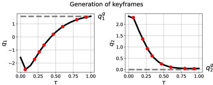
Figure 3: Generating keyframes (marked as red dots) from an optimal trajectory with $\boldsymbol{\theta}^{\text{true}}$. The gray dashed lines label the goal pose for each joint, i.e., $[q_{1}^{\text{g}},q_{2}^{\text{g}}]^{\mkern-1.5mu\mathsf{T}}=[\pi/2,0]^{\mkern-1.5mu\mathsf{T}}$.

TABLE I: Keyframes $\mathcal{D}$ generated in Fig. 3

. No. Time stamp $\tau_{i}$ ($T=1$) Keyframe $\boldsymbol{y}^{*}(\tau_{i})$ #1 $\tau_{1}=0.067$s $\boldsymbol{q}^{*}({\tau_{1}})=[-2.497,2.301]$ #2 $\tau_{2}=0.2$s $\boldsymbol{q}^{*}({\tau_{2}})=[-1.71,1.353]$ #3 $\tau_{3}=0.267$s $\boldsymbol{q}^{*}({\tau_{3}})=[-1.142,0.924]$ #4 $\tau_{4}=0.333$s $\boldsymbol{q}^{*}({\tau_{4}})=[-0.629,0.606]$ #5 $\tau_{5}=0.467$s $\boldsymbol{q}^{*}({\tau_{5}})=[0.201,0.25]$ #6 $\tau_{6}=0.6$s $\boldsymbol{q}^{*}({\tau_{6}})=[0.791,0.108]$ #7 $\tau_{7}=0.8$s $\boldsymbol{q}^{*}({\tau_{7}})=[1.319,0.049]$ #8 $\tau_{8}=0.933$s $\boldsymbol{q}^{*}({\tau_{8}})=[1.512,0.043]$

We choose different numbers of keyframes from Table I to learn the time-warping and cost functions, and the results are in Fig. 4. The left panel of Fig. 4 shows the loss (32) versus iteration, and the right shows the parameter error $\lVert\boldsymbol{\theta}-\boldsymbol{\theta}^{\text{true}}\rVert^{2}$ versus iteration.

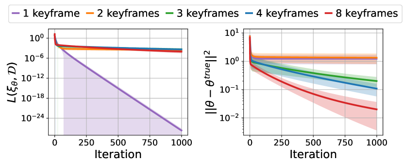
Figure 4: Learning from different numbers of keyframes. The left panel shows the loss (32) versus iteration, the right shows the parameter error $\lVert\boldsymbol{{\theta}}_{k}-\boldsymbol{{\theta}}^{\text{true}}\rVert^{2}$ versus iteration. The solid line and shaded area denote the mean and standard derivation over all 10 trials.

Fig. 4 shows that when the number of keyframes $N\geq 3$ (blue, green, and red lines), the loss $L(\boldsymbol{\xi}_{\boldsymbol{\theta}_{k}},\mathcal{D})$ and parameter error $\lVert\boldsymbol{{\theta}}_{k}-\boldsymbol{{\theta}}^{\text{true}}\rVert^{2}$ converge to zeros, indicating that both the cost and time-warping functions are successfully learned. When $N\leq 2$, while the loss converges to zero, $\boldsymbol{\theta}_{k}$ does not converge to $\boldsymbol{\theta}^{\text{true}}$ (orange and purple lines in the right panel). This indicates when $N\leq 2$, there are multiple cost and time-warping functions, besides $\boldsymbol{\theta}^{\emph{true}}$, that lead to the given keyframes. In other words, with fewer keyframes, we cannot uniquely determine the cost and time-warping functions, as they are over-parameterized relative to given keyframes. Intuitively, to uniquely determine $\boldsymbol{\theta}^{\text{true}}$, the number of constraints imposed by the given keyframes, $oN$ (recall $o$ is the dimension of $\boldsymbol{g}()$), should be no less than the number of all unknown parameters, $r{+}s$, that is, $N\geq\frac{r{+}s}{o}$. Please refer to Section VII-A for more analysis.

From the right panel of Fig. 4, we also observe that different numbers of keyframes ($N\geq 3$) also influence the converge rate. For instance, the convergence rate with 8 keyframes (red line) is faster than that of 4 keyframes (blue line). Since the proposed method updates the cost and time-warping functions by finding the deepest descent direction of loss, thus, the more keyframes are given, the better informed the gradient direction will be, making the convergence to the true parameters faster.

Lastly, we test the generalization of the learned cost and time-warping functions, by setting the robot arm to new initial state $\boldsymbol{x}(0)=[-\frac{\pi}{4},0,0,0]^{\mkern-1.5mu\mathsf{T}}$ and new horizon $T{=}2$ (both are very different from the ones in learning). The generated motion using the learned $\boldsymbol{\theta}$ (mean value over all trials) is shown in Fig. 5, where we have also plotted the trajectory of $\boldsymbol{\theta}^{\text{true}}$ for reference. To compare the generalization performance, we compute the distance between the final state $\boldsymbol{x}(T)$ of the generalized motion and the goal state $\boldsymbol{x}^{\text{g}}=[\frac{\pi}{2},0,0,0]^{\mkern-1.5mu\mathsf{T}}$, and list the results in Table II. Both Fig. 5 and Table II show that the learned $\boldsymbol{\theta}$ enables to generate new motion in unseen conditions. Further, Table II shows that the increasing keyframes could lead to better generalization. Notably, we see that although the learned $\boldsymbol{\theta}$s from 1 or 2 keyframes are different from $\boldsymbol{\theta}^{\text{true}}$, they can still obtain fair generalization. This could be due to the formulation of the distance-to-goal features (29). Although the learned weight vector $\boldsymbol{\theta}$ is different from $\boldsymbol{\theta}^{\text{true}}$, the distance-to-goal features largely contributes to a similar performance. We will show later in Section V-D that when (29) is replaced with a neural cost function, fewer keyframes will lead to poor generalization. Thus, for the same number of keyframes, different cost function formulations could lead to different generalization abilities. But as we will see in Section V-D, a common observation is that the more keyframes are given, the better the generalization will be for the learned cost function.

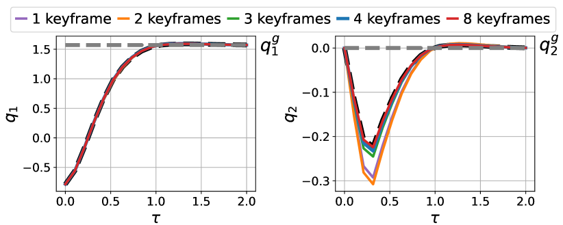
Figure 5: Generalization of the learned cost function given new initial condition $\boldsymbol{x}(0)$ and new horizon $T$. The gray dashed lines mark the goal for each joint $[q_{1}^{\text{g}},q_{2}^{\text{g}}]^{\mkern-1.5mu\mathsf{T}}=[\pi/2,0]^{\mkern-1.5mu\mathsf{T}}$.

TABLE II: Distance between the final state $\boldsymbol{x}(T)$ of the generalized motion and the goal $\boldsymbol{x}^{\text{g}}$, i.e., $\lVert\boldsymbol{x}(T)-\boldsymbol{x}^{\text{g}}\rVert$.

The learned $\boldsymbol{\theta}$ (mean value) from	$\lVert\boldsymbol{x}(T)-\boldsymbol{x}^{\text{g}}\rVert$
1 keyframe	$0.00581$
2 keyframes	$0.00580$
3 keyframes	$0.00392$
4 keyframes	$0.00382$
8 keyframes	$0.00358$
True $\boldsymbol{\theta}^{\text{true}}$	$\boldsymbol{0.00346}$

V-B Non-optimal Keyframes

Next, we evaluate the performance of the proposed method given non-optimal keyframes. This emulates the situation where a demonstration could be polluted by biased sensing error, noise, hardware error, etc. We select keyframes $\mathcal{D}$ by corrupting each keyframe in Fig. 4 with a biased error, as shown in the first column (red dots) of Fig. 6. We evaluate the performance of the method given such biased keyframes. The other experiment settings follow the previous experiment. We have run each experiment for 10 trials with different random seeds for the initial $\boldsymbol{\theta}_{0}$.

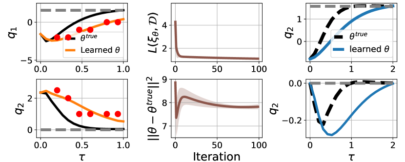
Figure 6: Learning from non-optimal keyframes. The first column shows the given keyframes (red dots), which deviate from the optimal trajectory (black lines), and the reproduced trajectory (orange lines) from the learned $\boldsymbol{\theta}$ (mean value over all 10 trials). The second column shows the loss and parameter error versus iteration; the solid line and shaded area denote the mean and standard derivation over all 10 trials. The third column shows the generalization of the learned $\boldsymbol{\theta}$ to new initial condition $\boldsymbol{x}(0)$ and new time horizon $T$. The gray dashed lines in the first and third columns mark the goal for each joint $[q_{1}^{\text{g}},q_{2}^{\text{g}}]^{\mkern-1.5mu\mathsf{T}}=[\pi/2,0]^{\mkern-1.5mu\mathsf{T}}$. As calculated in Table II, $\lVert\boldsymbol{x}(T)-\boldsymbol{x}^{\text{g}}\rVert$ for the generalized motion in the third column is 0.107.

In Fig. 6, the loss and parameter error versus iteration are shown in the top and bottom panels of the second column, respectively. The solid line and shaded area denote the mean and standard derivation over all 10 trials. We use the learned $\boldsymbol{\theta}$ to reproduce the optimal trajectory of the robot, which is shown in the first column (orange lines). In the third column, we test the generalization of the learned $\boldsymbol{\theta}$ to the new initial condition $\boldsymbol{x}(0)=[-\frac{\pi}{4},0,0,0]^{\mkern-1.5mu\mathsf{T}}$ and new horizon $T=2$. Here, we also compare with the trajectory of $\boldsymbol{\theta}^{\text{true}}$ (dashed black lines). From Fig. 6, we have the following comments.

Since the keyframes in the first column are non-optimal, there does not exist a $\boldsymbol{\theta}$ that exactly corresponds to those non-optimal keyframes. Thus, the loss in the second column does not converge to zero. Despite those, the method still finds a $\boldsymbol{\theta}$ such that its produced trajectory is closest to the keyframes, as shown by orange lines in the first column. The second column shows that the learned $\boldsymbol{\theta}$ is different from $\boldsymbol{\theta}^{\text{true}}$.

The generalization in the third column shows that given the new initial condition and horizon, the generalized motion still approaches the goal, and the final distance of the generalized motion to the goal is $\lVert\boldsymbol{x}(T)-\boldsymbol{x}^{\text{g}}\rVert=0.107$, which is larger compared to the one in Table II.

V-C Different Time-Warping Functions

In this set of experiments, we test the learning performance of using polynomial time-warping functions of different complexity. The keyframes $\mathcal{D}$ are the red dots in the first column of Fig. 6. For each polynomial time-warping function, we have run the experiment for 10 trials with different random seeds for initial $\boldsymbol{\theta}_{0}$. Other experiment settings follow the previous one. The results are summarized in Table III. Here, the first column shows the learned time-warping functions; the second column is the final converged losses, and the statistics (mean+standard deviation) are over 10 trials. We have the following comments.

TABLE III: Learning with different time-warping functions

Learned time-warping function	$\min L(\boldsymbol{\xi}_{\boldsymbol{\theta}},\mathcal{D})$ (mean$\pm$std)
$t=2.55\tau$	$1.017\pm 0.014$
$t=2.90\tau-0.55\tau^{2}$	$0.876\pm 0.008$
$t=2.94\tau+0.28\tau^{2}-0.88\tau^{3}$	$0.831\pm 0.006$
$t=2.89\tau+0.53\tau^{2}-0.49\tau^{3}-0.60\tau^{4}$	$0.822\pm 0.002$

Table III shows that a higher order of polynomial time-warping function leads to the lower final loss. This is because a higher degree polynomial introduces additional degrees of freedom, which enable to represent more complex time mapping and contribute to further decreasing the loss. Meanwhile, Table III shows that (i) the first-order terms in all learned time-warping polynomials are similar, (ii) the higher-order terms are relatively small compared to the first-order term, and (iii) adding higher-order terms to the time-warping polynomial only decreases a small amount of final loss. All those observations indicate that the first-order term dominates the final performance. We may conclude that in practice, it is preferable to start with a simplified time-warping function. The subsequent experiments will use the first-order time-warping function for simplicity.

V-D Learning Neural Cost Functions

In this session, we test the ability of the proposed method to learn neural-network cost functions. This is useful if a weight-feature cost function formulation cannot be specified due to the lack of prior knowledge. We set the cost function (29) with the following neural-network cost function,

$$c(\boldsymbol{x},\boldsymbol{u},{\boldsymbol{p}}) =\boldsymbol{\phi}_{\boldsymbol{p}}^{\mkern-1.5mu\mathsf{T}}(\boldsymbol{x})\boldsymbol{\phi}_{\boldsymbol{p}}(\boldsymbol{x})+0.05\lVert\boldsymbol{u}\rVert^{2},$$ (34)

$$h(\boldsymbol{x},{\boldsymbol{p}}) =\boldsymbol{\phi}_{\boldsymbol{p}}^{\mkern-1.5mu\mathsf{T}}(\boldsymbol{x})\boldsymbol{\phi}_{\boldsymbol{p}}(\boldsymbol{x}),$$

where $\boldsymbol{\phi}_{\boldsymbol{p}}(\boldsymbol{x})$ is a 4-8 fully-connected neural network [54] (i.e., 4-neuron input layer and 8-neuron output layer), and $\boldsymbol{p}\in\mathbb{R}^{40}$ is the parameter of the neural network, i.e., all weight matrices and bias vectors. Note that (34) uses dot product in the output layer of the neural network to guarantee the positiveness of the cost function. The time-warping polynomial has the degree of one. We use the keyframes in Fig. 3 (also in Table I). Other experiment settings are the same as the previous ones. In each evaluation case below, we have run the experiment for 10 trials with different random seeds for the initial $\boldsymbol{\theta}_{0}$.

We plot the learning and generalization results in Fig. 7. We test with three cases of the keyframes shown in red dots in the second row, and the corresponding results are shown in each column. In each case, the first row shows the loss versus iteration; and second and third rows show the reproduced trajectories (orange lines) by the learned cost and time-warping functions; and the fourth and fifth rows show the generalization (blue lines) of the learned cost function to new initial state $\boldsymbol{x}(0)=[-\frac{\pi}{4},0,0,0]^{\mkern-1.5mu\mathsf{T}}$ and new horizon $T=2$. The motion (dashed black lines) of $\boldsymbol{\theta}^{\text{true}}$ is also plotted for reference. In Table IV, we compute the distance between $\boldsymbol{x}(T)$ of the generalized motion and the goal $\boldsymbol{x}^{\text{g}}=[\frac{\pi}{2},0,0,0]^{\mkern-1.5mu\mathsf{T}}$ to measure the generalization performance. We have the following comments.

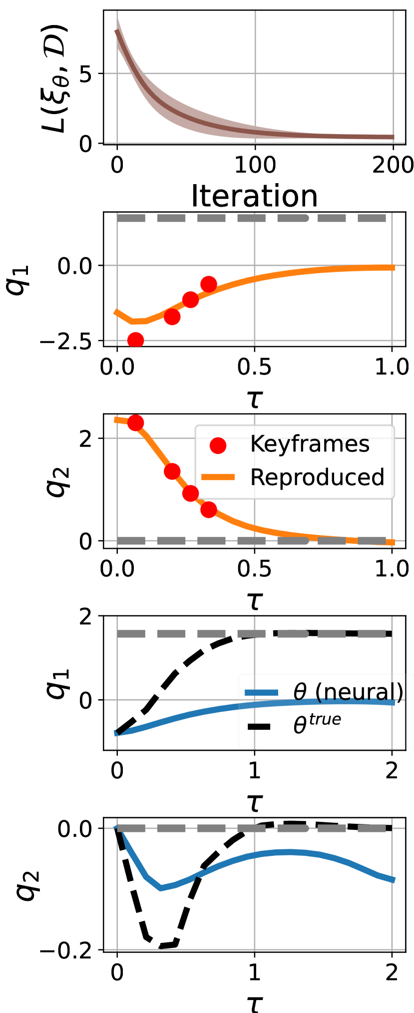
(a) Case 1

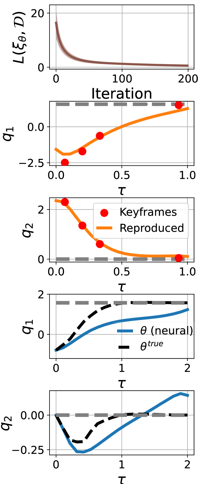
(b) Case 2

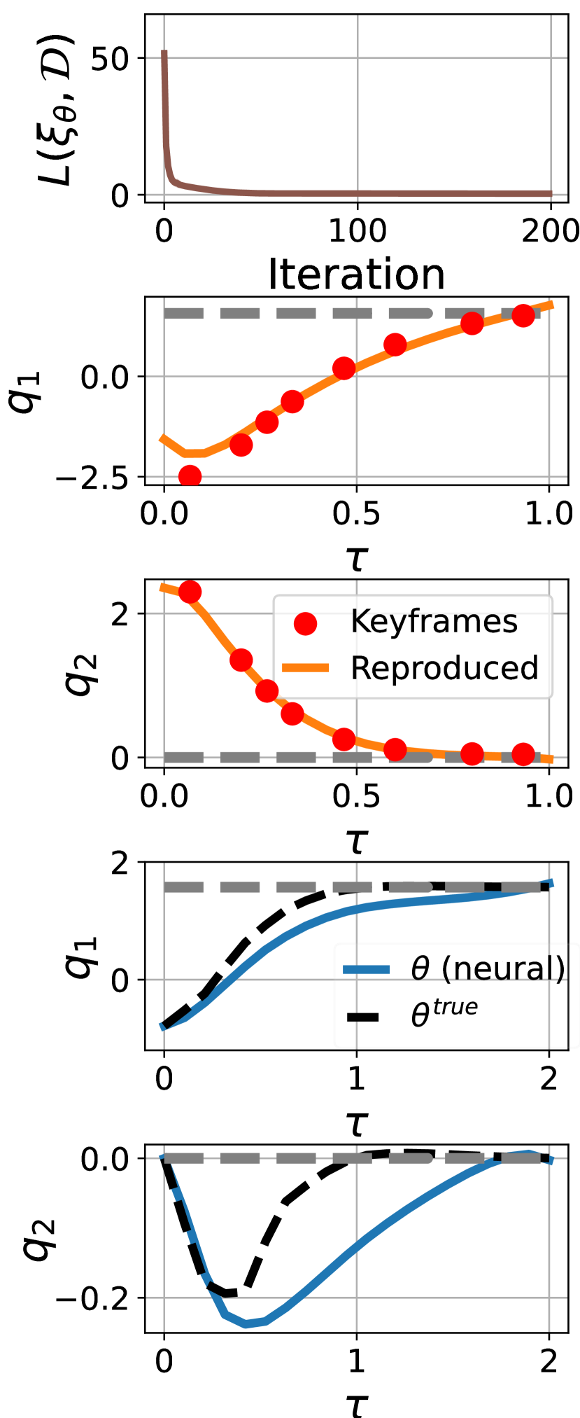
(c) Case 3

Figure 7: Learning neural cost functions from keyframes. Three cases of keyframes are used, shown in the red dots in each column. In each case, the first row shows loss versus iteration (the solid line and shaded area denote the mean and standard derivation over all 10 trials). The second and third rows show the reproduced trajectories (orange lines) of the learned $\boldsymbol{\theta}$. The fourth and fifth rows show the generalization (blue lines) of the learned $\boldsymbol{\theta}$ to new initial state and horizon, and the motion (dashed black lines) of $\boldsymbol{\theta}^{\text{true}}$ is also plotted for reference. In second-fifth rows, the gray dashed lines mark the goal for each joint $[q_{1}^{\text{g}},q_{2}^{\text{g}}]^{\mkern-1.5mu\mathsf{T}}=[\pi/2,0]^{\mkern-1.5mu\mathsf{T}}$.

TABLE IV: Distance of $\boldsymbol{x}(T)$ of the generalized motion (in the fourth and fifth rows in Fig. 7) to goal $\boldsymbol{x}^{\text{g}}=[\frac{\pi}{2},0,0,0]^{\mkern-1.5mu\mathsf{T}}$.

The learned $\boldsymbol{\theta}$ (mean value over all trials)	$\lVert\boldsymbol{x}(T)-\boldsymbol{x}^{\text{g}}\rVert$
Case 1	$1.638$
Case 2	$0.717$
Case 3	$0.388$
True $\boldsymbol{\theta}^{\text{true}}$	$\boldsymbol{0.00346}$

First, compared to the distance-to-goal cost (29), the neural cost (34) is goal-blind, meaning that the goal $\boldsymbol{q}^{\text{g}}=[\frac{\pi}{2},0]^{\mkern-1.5mu\mathsf{T}}$ is not encoded in the neural cost function before training. Thus, it is crucial for the robot to learn a goal-encoded neural cost for the success of the task. Case 1 and Case 2 use four keyframes to learn a cost function. The results in fourth and fifth rows of Fig. 7 and in Table IV indicate that Case 2 has a better generalization than Case 1 does: Case 2 has a final distance $\lVert\boldsymbol{x}(T)-\boldsymbol{x}^{\text{g}}\rVert{=}0.717$, while Case 1 has $\lVert\boldsymbol{x}(T)-\boldsymbol{x}^{\text{g}}\rVert{=}1.638$. This is because the keyframes in Case 1 are mainly clustered at the beginning of motion, and thus cannot provide sufficient information about the final goal. In contrast, Case 2 has a keyframe at the goal, and thus the learned neural cost function captures such goal information.

Second, we add more keyframes in Case 3. It shows that more keyframes lead to better generalization of the learned neural cost function: the final distance is $\lVert\boldsymbol{x}(T)-\boldsymbol{x}^{\text{g}}\rVert=0.388$, which is better than those in Case 2 and Case 1.

Lastly, the learned neural cost function in Case 2 or Case 3, while controlling the robot to approach the goal, has a trajectory that is different from the true one (black dashed lines). This manifests the generalizability of learning cost functions. We also note that the neural cost function (34) is over-parameterized, relative to the fewer given keyframes. Despite this, the learned neural cost still shows a fair generalization to new motion conditions, given a proper selection of keyframes.

V-E Comparison with Related Methods

In this session, we compare the proposed method with the related work. For all comparisons below, the learning process uses the keyframe data in Fig. 3 (Table I). The generalization is tested by setting the robot to a new initial condition $\boldsymbol{x}(0)=[-\frac{\pi}{4},0,0,0]^{\mkern-1.5mu\mathsf{T}}$ and a new time horizon $T=2$. Other settings follow the previous experiments if not explicitly stated.

V-E1 Comparison with Kinematic Learning [41]

Following [41], we fit the keyframes in Table I with a fifth-order spline, as shown in the brown lines in Fig. 8(a). The fitted spline is then used to generalize the robot motion in the new condition (i.e., a new initial condition and a new horizon). To do this, following the idea of [41], we compare which given keyframe is closest to the new $\boldsymbol{x}(0)$, then from which we perform extrapolation based on the fitted spline to generate the new trajectory over the new horizon $T=2$. The generated trajectories are plotted in Fig. 8(b). For comparison, we also plot the generalized motion of the previously learned weighted cost (29) and neural cost (34) in Fig. 8(c). We have the following comments on the results.

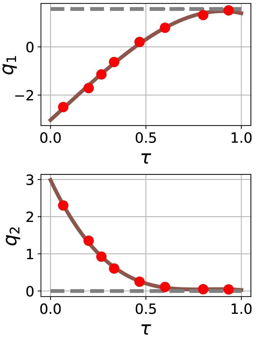
(a) Spline fitting to the keyframes [41]

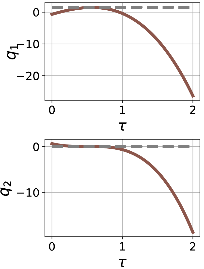
(b) Generalization of the fitted spline [41]

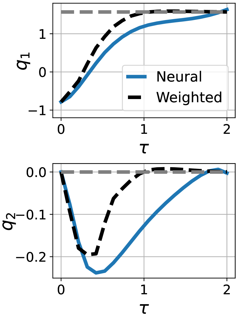
(c) Generalization for the proposed method

Figure 8: Comparison between [41] and the proposed method. (a) is the spline model fitted to keyframes; (b) is the generalization of the fitted spline in new motion condition (new $\boldsymbol{x}(0)$ and new $T$); and (c) is the generalization of the learned weighted cost function (29) and learned neural cost function (34) in the previous experiments. The gray dashed lines mark the goal of each joint $[q_{1}^{\text{g}},q_{2}^{\text{g}}]^{\mkern-1.5mu\mathsf{T}}=[\pi/2,0]^{\mkern-1.5mu\mathsf{T}}$. The final distance $\lVert\boldsymbol{x}(T)-\boldsymbol{x}^{\text{g}}\rVert$ of the generalized motion is 33.670 for the fitted spline in (b), 0.388 for the learned neural cost function in (c), and 0.00358 for the learned weighted cost function in (c).

First, the spline function fits well to the keyframes (red dots in Fig. 8(a)). However, the generalization of the obtained spline model is poor: the generalized motion has a final distance of 33.670 to the goal. The poor performance is because the spline is only a local kinematic model, and it cannot generalize motion that is far away from the keyframes.

Second, given the same number of keyframes, learning cost functions shows evident advantage in generalization. As in Fig. 8(c), both the learned weighted cost function and neural cost function can successfully control the robot to reach the goal in new conditions. The reason why cost functions have superior performance is that a cost function is a compact representation of robot motion, and it represents a space of motion trajectories parameterized by different initial conditions and time horizons. Previous work [1] had the same conclusion.

V-E2 Comparison with Numerical Differentiation

Recall that a key technique of the Continuous PDP is Differential Pontryagin’s Maximum Principle, which efficiently computes the analytic gradient of the trajectory of a continuous-time optimal control system with respect to system parameters. An alternative is numerical differentiation, that is, one uses numerical differentiation to obtain $\frac{dL}{d\boldsymbol{\theta}}$. The experiments below compare those two options. Other experiment settings are the same as the previous ones.

Consider the neural cost function in (34). We vary the size of the neural network, i.e., the dimension of $\boldsymbol{p}$, and the system time horizon $T$. We compare the computation time needed to compute $\frac{dL}{d\boldsymbol{\theta}}$ by Continuous PDP and numerical differentiation. The results are in Fig. 9, based on which we have the following comments.

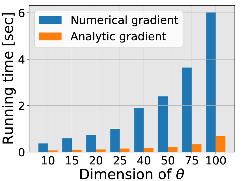
(a) Varying parameter dimension

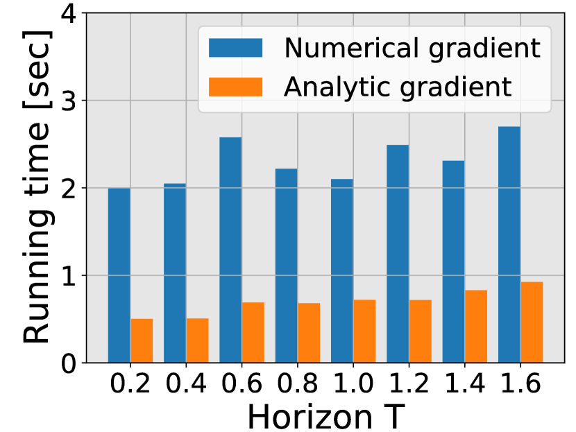
(b) Varying system horizon

Figure 9: Comparison of computation time between numerical differentiation and Continuous PDP.

Fig. 9(a) shows an exponential increase of computational time of numerical differentiation when the number of system parameters (dimension of $\boldsymbol{\theta}$) increases. This is because numerical differentiation requires evaluating the loss by perturbing the parameter vector in each dimension. Each perturbation and evaluation require solving an optimal control problem once, thus causing high-computational cost for high-dimensional $\boldsymbol{\theta}$. In contrast, the Continuous PDP solves analytical gradients by performing the Riccati-type iteration (Lemma 1). Since there is no need to repetitively solve optimal control problems during the differentiation, the proposed method can handle the large-scale optimization problem, such as $\boldsymbol{\theta}\in\mathbb{R}^{100}$ in Fig. 9(a).

Fig. 9(b) shows the comparison results given different system horizons. One observation is that the complexity of Continuous PDP is approximately linear to the system horizon $T$. This is because the numerical integration of the Riccati-type equations in Lemma 1 is linear to the horizon $T$.

V-E3 Comparison with [31]

In this part, we compare the proposed method with [31]. As discussed in the related work, [31] formulates a problem similar to (16) which also minimizes a trajectory discrepancy loss (32), but the authors solve it by replacing the inner optimal control problem with the Pontryagin’s Maximum Principle conditions, thus turning a bi-level optimization into a plain constrained optimization. We compare their method with the Continuous PDP in terms of convergence, sensitivity to different initialization, and generalization.

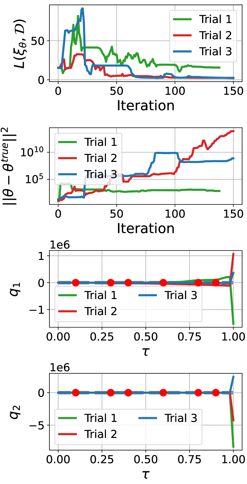
(a) The method in [31].

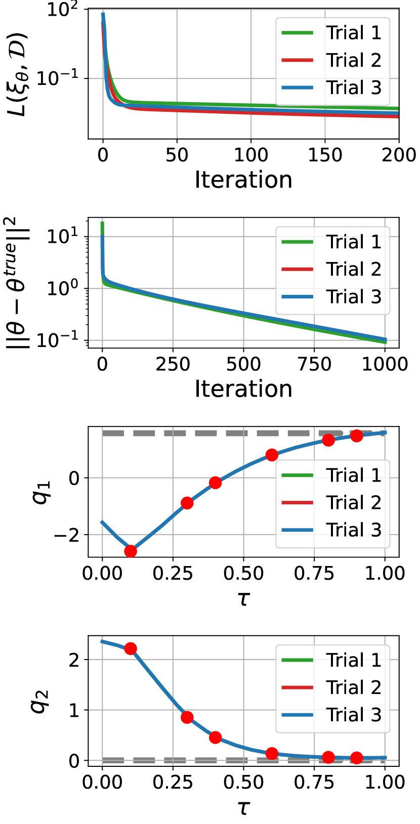
(b) The proposed method.

Figure 10: Comparison between the method in [31] (a) and the proposed method (b). Each method has three trials using different initial guesses $\boldsymbol{\theta}_{0}$, and at each trial, both methods start from the same $\boldsymbol{\theta}_{0}$. Different trials are shown in different color. The first and second rows show the loss and parameter error versus iteration, respectively. The third and fourth rows show the reproduced trajectory of the learned $\boldsymbol{\theta}$. For [31], the converted plain optimization is solved by IPOPT [55]. Gray dashed lines mark the goal of each joint $[q_{1}^{\text{g}},q_{2}^{\text{g}}]^{\mkern-1.5mu\mathsf{T}}=[\pi/2,0]^{\mkern-1.5mu\mathsf{T}}$.

Both methods use the same keyframes shown in the third and fourth rows in Fig. 10, first-order polynomial time-warping function (30), and the cost function parameterization (29). Other experiment settings are the same as the previous experiments unless explicitly stated. Fig. 10 presents the results of [31] (left) and the proposed method (right). Here, each method has three trials from different initial guesses $\boldsymbol{\theta}_{0}$ (i.e., using different random seeds). Different trials are shown in different colors. The first and second rows plot the loss and parameter error versus iteration, respectively. The third and fourth rows show the reproduced trajectories with the learned $\boldsymbol{\theta}$. We have the following comments.

First, following [31], the converted plain optimization has 504 constraint equations and 509 decision variables. This is large-scale and non-convex optimization, and we used IPOPT [55] to solve it. But IPOPT is very likely to get stuck to local optima for this problem. This has been illustrated by Fig. 10(a): the loss has converged to a small value, but the learned $\boldsymbol{\theta}$ is far away from $\boldsymbol{\theta}^{\text{true}}$. Also, in the third and fourth rows, although the produced trajectories are close to the keyframes (red dots), they are very different from the ground truth in Fig. 3.

The proneness of [31] to get stuck to bad solutions could be due to two main reasons. First, since Pontryagin’s Maximum Principle is just a necessary condition, the solutions that satisfy this condition may include the saddle points, which might not necessarily be the solution to the original optimal control problem. Thus, such a problem reformulation is not equivalent to the original bi-level problem in general. Second, the converted plain optimization can be large-scale and highly nonlinear. If not properly initialized, it would easily get stuck into a local solution.

In contrast, the proposed method solves the problem by maintaining the bi-level structure. This bi-level treatment leads to more numerical tractability. The lower-level optimal control problem can be solved by many available trajectory optimization methods such as iLQR [47], DDP [48], and the upper level uses gradient-descent. Also, the bi-level treatment can lead to better performance in finding good (if not global) solutions. As empirically shown in Fig. 10(b), with various random guesses $\boldsymbol{\theta}_{0}$s, the proposed method all converges to the true $\boldsymbol{\theta}^{\text{true}}$.

Finally, we need to mention that in the Continuous PDP, Pontryagin’s Maximum Principle is only used for differentiating the trajectory of the optimal control system, not replacing the optimal control system. In other words, the trajectory has to be computed on the lower level before its differentiation can be done. Therefore, the proposed method in this paper is fundamentally different from [31].

VI Learning from Keyframes for planning in unknown environments

This section presents an application scenario of the proposed method: a robot learns a motion planner from demonstrated keyframes to navigate through an unknown environment. A user provides a few keyframes in the vicinity of obstacles in an environment, and a robot learns a cost function from those keyframes such that its produced motion can avoid the obstacles. Experiments in this section are based on a 6-DoF quadrotor. The code can be accessed at https://github.com/wanxinjin/Learning-from-Sparse-Demonstrations. A real-world demonstration is given at https://youtu.be/BYAsqMxW5Z4.

VI-A 6-DoF Quadrotor Setup

The equation of motion of a quadrotor flying in $SE(3)$ (full position and attitude) space is given by

$$\dot{\boldsymbol{r}}_{I} {={\boldsymbol{v}}_{I}},$$ (35a)

$$m\dot{\boldsymbol{v}}_{I} =m\boldsymbol{g}_{I}+\boldsymbol{f}_{I},$$ (35b)

$$\dot{\boldsymbol{q}}_{B/I} =\frac{1}{2}\Omega(\boldsymbol{\omega}_{B}){\boldsymbol{q}}_{B/I},$$ (35c)

$$J_{B}\dot{\boldsymbol{\omega}}_{B} =\boldsymbol{\tau}_{B}-\boldsymbol{\omega}_{{B}}\times J_{B}\boldsymbol{\omega}_{B}.$$ (35d)

Here, the subscripts _B and _I denote a quantity expressed in the body and world coordinate frames, respectively; $m$ is the quadrotor mass; $\boldsymbol{r}_{I}=[r_{x},r_{y},r_{z}]^{\mkern-1.5mu\mathsf{T}}\in\mathbb{R}^{3}$ and $\boldsymbol{v}_{I}\in\mathbb{R}^{3}$ are the quadrotor’s position and velocity, respectively; $J_{B}\in\mathbb{R}^{3\times 3}$ is the moment of inertia; $\boldsymbol{\omega}_{B}\in\mathbb{R}^{3}$ is the angular velocity; $\boldsymbol{q}_{B/I}\in\mathbb{R}^{4}$ is the unit quaternion [56] describing the attitude of the quadrotor with respect to the world frame; (35c) is the quaternion calculus, and $\Omega(\boldsymbol{\omega}_{B})$ is the matrix of $\boldsymbol{\omega}_{B}$ for quaternion multiplication [56]; $\boldsymbol{\tau}_{B}\in\mathbb{R}^{3}$ is the torque vector applied to the quadrotor; and $\boldsymbol{f}_{I}\in\mathbb{R}^{3}$ is the total force vector. The net force magnitude $\lVert\boldsymbol{f}_{I}\rVert={{f}}\in\mathbb{R}$ (along the z-axis of the body frame) and torque $\boldsymbol{\tau}_{B}=[\tau_{x},\tau_{y},\tau_{z}]$ are generated by thrust $[T_{1},T_{2},T_{3},T_{4}]$ of four propellers via

$$\begin{bmatrix}{{f}}\\ \tau_{x}\\ \tau_{y}\\ \tau_{z}\end{bmatrix}=\begin{bmatrix}1&1&1&1\\ 0&-l_{\text{w}}/2&0&l_{\text{w}}/2\\ -l_{\text{w}}/2&0&l_{\text{w}}/2&0\\ \kappa&-\kappa&\kappa&-\kappa\end{bmatrix}\begin{bmatrix}T_{1}\\ T_{2}\\ T_{3}\\ T_{4}\end{bmatrix},$$ (36)

with $l_{\text{w}}$ the wing length of the quadrotor and $\kappa$ a fixed constant. In our experiment, the gravity constant is $10\text{m/s}^{2}$ and all other dynamics parameters are units. The state vector is $\boldsymbol{x}=[\boldsymbol{r}_{I}^{\mkern-1.5mu\mathsf{T}},\boldsymbol{v}_{I}^{\mkern-1.5mu\mathsf{T}},\boldsymbol{q}_{B/I}^{\mkern-1.5mu\mathsf{T}},\boldsymbol{\omega}_{B}^{\mkern-1.5mu\mathsf{T}}]^{\mkern-1.5mu\mathsf{T}}\in\mathbb{R}^{13}$ and the control vector is $\boldsymbol{u}=[T_{1},T_{2},T_{3},T_{4}]^{\mkern-1.5mu\mathsf{T}}\in\mathbb{R}^{4}.$

To achieve ${SE(3)}$ maneuvering, we need to carefully design the attitude error. Following [57], we define the attitude error between the current attitude $\boldsymbol{q}$ and goal $\boldsymbol{q}^{\text{g}}$ as

$$e(\boldsymbol{q},\boldsymbol{q}_{\text{g}})=\frac{1}{2}\text{trace}(I-R^{\mkern-1.5mu\mathsf{T}}(\boldsymbol{q}^{\text{g}})R(\boldsymbol{q})),$$ (37)

where $R(\boldsymbol{q})\in\mathbb{R}^{3\times 3}$ is the rotation matrix corresponding to quaternion $\boldsymbol{q}$ (see [56] for more details). For the cost function formulation (2), we use a generic polynomial function:

$$c({\boldsymbol{x},\boldsymbol{u}},{\boldsymbol{p}}){=} p_{1}r_{x}^{2}+p_{2}r_{y}^{2}+p_{3}r_{z}^{2}+p_{4}r_{x}+p_{5}r_{y}+p_{6}r_{z}$$

$$+p_{7}r_{x}r_{y}+p_{8}r_{x}r_{z}+p_{9}r_{y}r_{z}+0.1\lVert\boldsymbol{u}\rVert^{2},$$ (38a)

$$h({\boldsymbol{x}}){=} 10\lVert\boldsymbol{r}_{I}{-}\boldsymbol{r}_{I}^{\text{g}}\rVert^{2}+5\lVert\boldsymbol{v}_{I}\rVert^{2}+$$

$$100e(\boldsymbol{q}_{B/I},\boldsymbol{q}_{B/I}^{\text{g}})+5\lVert\boldsymbol{\omega}_{B}\rVert^{2},$$ (38b)

where $\boldsymbol{r}_{I}=[r_{x},r_{y},r_{z}]^{\mkern-1.5mu\mathsf{T}}$ is the quadrotor’s position, and we have fixed the final cost $h(\boldsymbol{x})$ since the quadrotor is always expected to land near a goal position $\boldsymbol{r}_{I}^{\text{g}}$ with goal attitude $\boldsymbol{q}_{B/I}^{\text{g}}$; and the goal velocities here are zeros. The cost function parameter $\boldsymbol{p}=[p_{1},p_{2},p_{3},p_{4},p_{5},p_{6},p_{7},p_{8},p_{9}]^{\mkern-1.5mu\mathsf{T}}\in\mathbb{R}^{9}$ will determine how the quadrotor reaches the goal (i.e., the specific flying trajectory of the quadrotor).

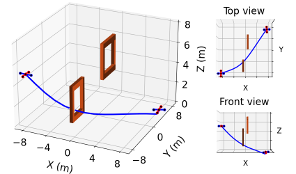
Figure 11: Quadrotor flying in an environment with obstacles. The goal is to let the quadrotor to fly from the left, go through the two gates (from left to right), and finally land near the goal position on the right with goal attitude. The plotted trajectory is a planned motion with a random cost function, which fails to achieve the goal.

As shown in Fig. 11, we aim the quadrotor to fly from the left initial position $\boldsymbol{r}_{I}(0)$ with $\boldsymbol{v}_{I}(0)$, $\boldsymbol{q}_{B/I}(0)$, and $\boldsymbol{\omega}_{B}(0)$, sequentially pass through two gates (from left to right gates), and finally land near the goal position $\boldsymbol{r}_{I}^{\text{g}}$ with goal attitude $\boldsymbol{q}_{B/I}^{\text{g}}$ on the right. With a random cost function, the quadrotor trajectory (blue line) does not meet the task requirement.

VI-B Learning from Keyframes

TABLE V: Keyframes $\mathcal{D}$ for the quadrotor.

Keyframe #	Time stamp $\tau_{i}$	Keyframe $\boldsymbol{y}^{*}(\tau_{i})$
#1	$\tau_{1}=0.1$s	$\boldsymbol{r}_{I}({\tau_{1}})=[-4,-6,3]$
#2	$\tau_{2}=0.2$s	$\boldsymbol{r}_{I}({\tau_{2}})=[1,-6,3]$
#3	$\tau_{3}=0.4$s	$\boldsymbol{r}_{I}({\tau_{3}})=[1,-1,4]$
#4	$\tau_{4}=0.6$s	$\boldsymbol{r}_{I}({\tau_{4}})=[-1,1,5]$
#5	$\tau_{5}=0.8$s	$\boldsymbol{r}_{I}({\tau_{5}})=[2,3,4]$
	horizon $T=1$s

We arbitrarily choose five keyframes near the two gates, listed in Table V. Here, ‘arbitrarily’ means that we do not know whether these keyframes are realizable by an exact cost function. Without much deliberation, we assign a time stamp to each keyframe, such that they are (almost) evenly spaced in the time horizon $[0,T]$ (later we will also test the method given the random assignment of the time stamps). We also do not know whether $\tau_{i}$ and $T$ are achievable for the quadrotor dynamics. The keyframes here contain only position information, i.e.,

$$\boldsymbol{r}_{I}=\boldsymbol{y}=\boldsymbol{g}(\boldsymbol{x},\boldsymbol{u})$$ (39)

The time-warping function is the first-order polynomial function (30), and loss $L(\boldsymbol{\xi}_{\boldsymbol{{\theta}}},\mathcal{D})$ is in (32). The learning rate is $\eta{=}10^{-2}$. The quadrotor’s initial state is $\boldsymbol{r}_{I}(0)=[{-}8,{-}8,5]^{\mkern-1.5mu\mathsf{T}}$, $\boldsymbol{q}_{B/I}(0)=[1,0,0,0]^{\mkern-1.5mu\mathsf{T}}$, $\boldsymbol{v}_{I}(0)=[15,5,{-}10]^{\mkern-1.5mu\mathsf{T}}$, and $\boldsymbol{\omega}_{B}(0)=\boldsymbol{0}$. The goal position is $\boldsymbol{r}_{I}^{\text{g}}=[8,8,0]^{\mkern-1.5mu\mathsf{T}}$ and the goal attitude $\boldsymbol{q}_{B/I}^{\text{g}}=[1,0,0,0]^{\mkern-1.5mu\mathsf{T}}$ (recall the goal velocities here are zeros).

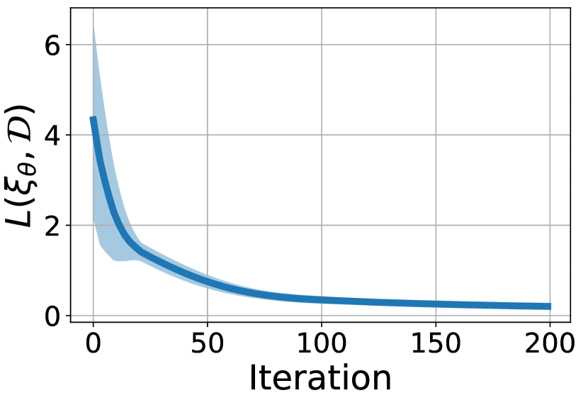
(a) Loss for Fig. 13(a)

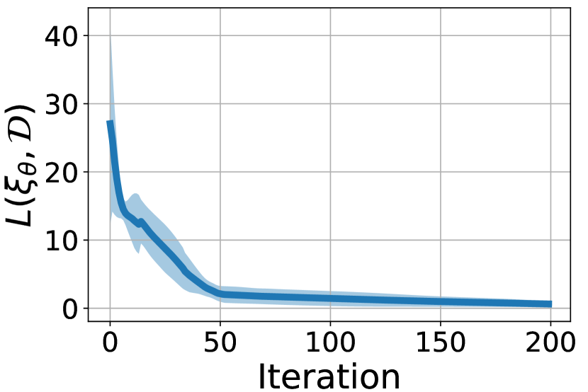
(b) Loss for Fig. 13(b)

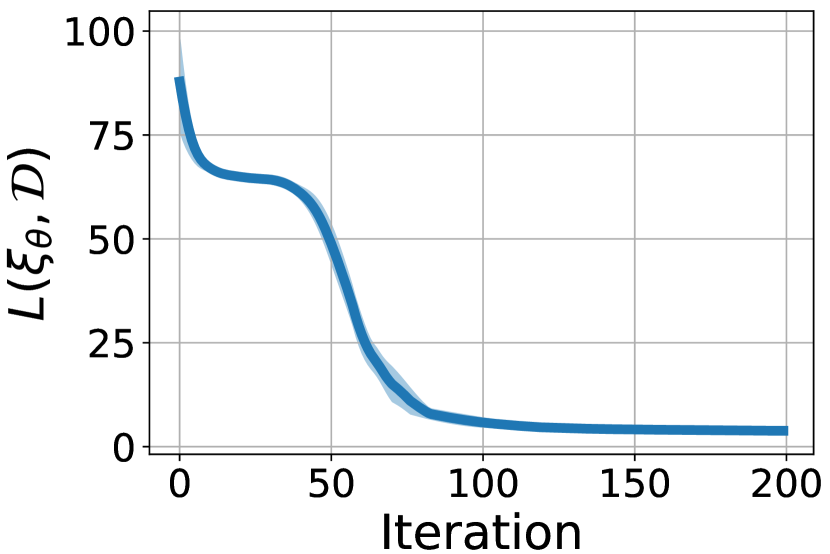
(c) Loss for Fig. 13(c)

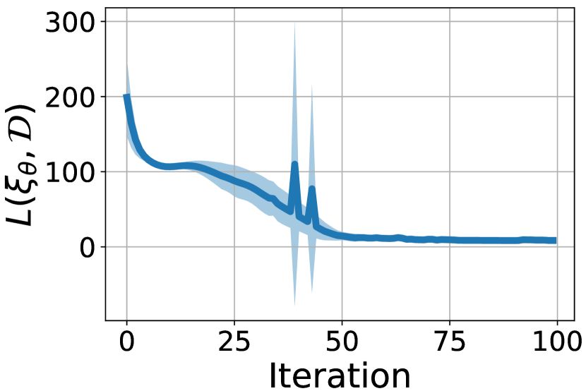
(d) Loss for Fig. 13(d)

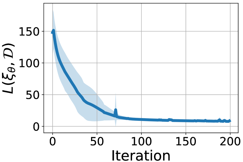
(e) Loss for Fig. 13(e)

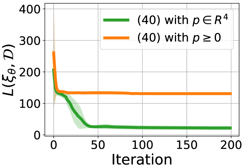
(f) Loss for Fig. 13(f)

Figure 12: Loss versus iteration, corresponding to different cases in Fig. 13. In each case, the solid line and shaded area denote the mean and standard derivation over 10 trial of the experiment, respectively. The final loss (mean+std) for each case is: $0.203\pm 0.035$ in (a), $0.625\pm 0.470$ in (b), $3.819\pm 0.805$ in (c), $8.548\pm 0.880$ in (d), $8.647\pm 2.022$ in (e), $21.777\pm 6.608$ for $\boldsymbol{p}\in\mathbb{R}^{4}$ and $130.902\pm 0.006$ for $\boldsymbol{p}\geq\boldsymbol{0}$ in (f).

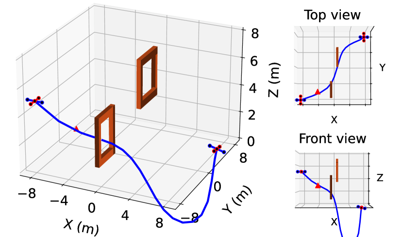
(a) Learning from keyframe #1.

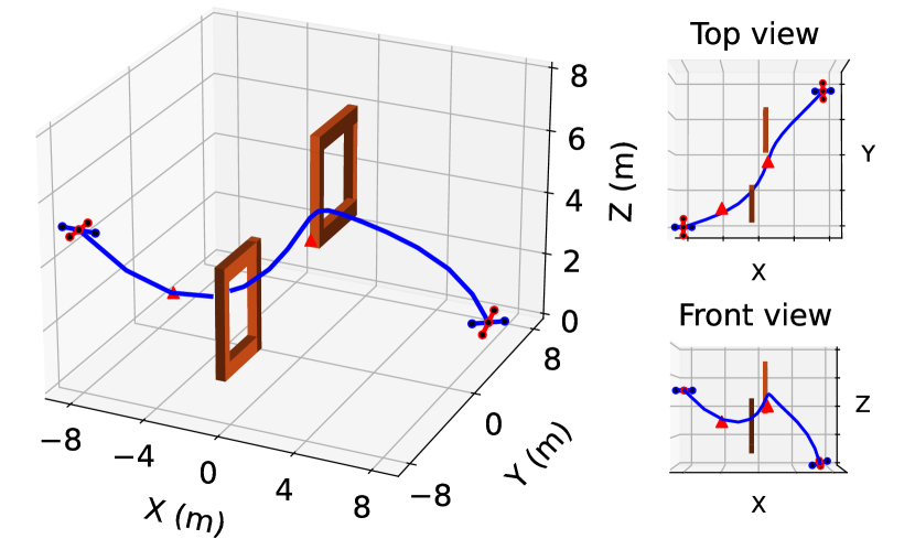
(b) Learning from keyframes #1 and #3.

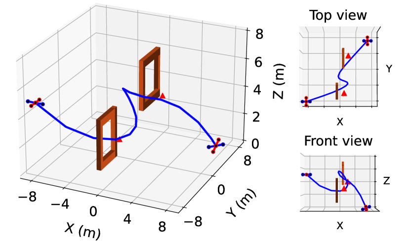
(c) Learning from keyframes #2 and #5.

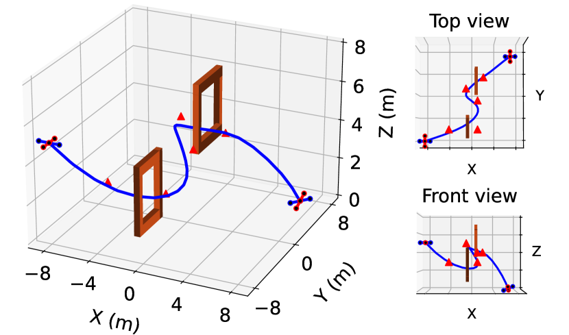
(d) Learning from keyframes #1-#5.

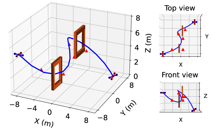
(e) Keyframes #1-#5 with random stamps.

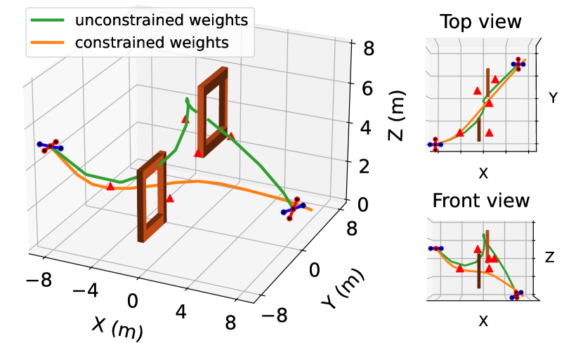
(f) Learning (40) from keyframes #1-#5.

Figure 13: Learning from keyframes given in Table V. (13(a))-(13(d)) show the reproduced trajectories by the cost functions learned from different number of keyframes. (13(e)) shows the case where we randomize the time stamp $\tau_{i}$ of each keyframe in Table V. (13(f)) shows the reproduced motion of the learned distance-to-obstacle cost function (40); here the green line corresponds to the unconstrained weights subcase, i.e., $\boldsymbol{p}\in\mathbb{R}^{4}$, and the orange to the constrained weights subcase, i.e., $\boldsymbol{p}\geq\boldsymbol{0}$. Corresponding to each of the above-mentioned figures, the loss versus iteration is given in Fig. 12.

VI-B1 Varying Number of Keyframes

Fig. 12(a)-12(d) and Fig. 13(a)-13(d) show different cases where we learn a cost function from different numbers of keyframes. In each case, we have run each experiment case for 10 trials, with each trial using different random seeds for the initial $\boldsymbol{\theta}_{0}$. Fig. 12(a)-12(d) plot the loss $L(\boldsymbol{\xi}_{\boldsymbol{{\theta}}},\mathcal{D})$ versus iteration, and Fig. 13(a)-13(d) show the reproduced trajectory using the learned cost and time-warping functions. We have the following comments on the results.

Fig. 13(a)-13(d) show that given keyframes in different locations, the proposed method always finds a cost function and a time-warping function such that the quadrotor’s reproduced motion can get close to the keyframes. Fig. 13(a)-13(d) also show that by increasing the number of keyframes and putting the keyframes around the gates, the quadrotor can successfully learn a cost function to fly through the two gates. Since the keyframes are arbitrarily placed and exact cost and time-warping functions (in the parameterization) may not exist, the final losses are not zeros as in Fig. 12(a)-12(d). Recall that we only make the path cost tunable, while the final cost given and fixed. Different placement of keyframes leads to different learned path costs and thus different motion trajectories. This cost formulation can be useful for learning how to move instead of where to move.

VI-B2 Random Time Stamps

In Fig. 13(e) and Fig. 12(e), we randomize the time stamp $\tau_{i}$ of each keyframe in Table V (drawn from a uniform distribution), and the cost function is learned from the randomly-timed keyframes. The other settings follow the previous experiment. Fig. 12(e) plots the loss versus iteration, and Fig. 13(e) show the reproduced trajectory from the learned cost and time-warping functions.

Comparing Fig. 13(d) and Fig. 13(e) with Fig. 12(d) and Fig. 12(e), respectively, we can see that the choice of time stamps of keyframes does not affect too much the learning: the final loss (mean+std) is $8.548\pm 0.880$ for Fig. 13(d) and $8.647\pm 2.022$ for Fig. 13(e). This result is understandable because whatever the keyframe time is, the proposed method always learns a time-warping function, which maps demonstration time to the robot dynamics time; thus performance of robot execution will not change significantly. The results show the importance of using a time-warping function in general LfD problems. The ability to handle the time misalignment is one of the key features of the proposed method.

VI-B3 Distance-to-Obstacle Cost Parameterization

In Fig. 13(f) and Fig. 12(f), we replace the polynomial cost function (38a) with the following distance-to-obstacle cost function:

$$c({\boldsymbol{x},\boldsymbol{u}},{\boldsymbol{p}}){=}-\sum_{i=1}^{4}p_{i}\lVert\boldsymbol{r}_{I}-\boldsymbol{o}_{i}\rVert^{2}+0.1\lVert\boldsymbol{u}\rVert^{2},$$ (40)

where the given $\boldsymbol{o}_{i}$ is the obstacle $i$’s position, which is the position of the left and right pillars of the two gates, shown in Fig. 11; and $\boldsymbol{p}\in\mathbb{R}^{4}$ are the weights for each to-obstacle distance $\lVert\boldsymbol{r}_{I}-\boldsymbol{o}_{i}\rVert^{2}$. We learn (40) from the five keyframes in Table V. Other experiment settings follow the previous session. We further divide the experiment into two subcases: In the first subcase (green line), we treat the weights $\boldsymbol{p}$ as unconstrained variables (i.e., it could be $\boldsymbol{p}\leq\boldsymbol{0}$, the obstacles could have an ‘attracting’ effect on quadrotor motion); and in the second subcase (orange line), we force $\boldsymbol{p}\geq\boldsymbol{0}$. The loss for those two subcases are plotted in Fig. 12(f), and the reproduced trajectories of the learned cost functions are in Fig. 13(f), where the green line corresponds to the unconstrained weights subcase while the orange to the constrained weights subcase.

In the unconstrained weights subcase in Fig. 13(f), one observation is that the motion (green line) is similar to the motion in Fig. 13(d) and Fig. 13(e). In fact, the learned weights are $\boldsymbol{p}{=}[-0.806,-1.406,-2.578,-2.246]^{\mkern-1.5mu\mathsf{T}}{\leq}\boldsymbol{0}$. This indicates that each obstacle has an attracting effect on the quadrotor’s motion. Considering the distance-to-obstacle cost in (40) is a second-order polynomial function in $\boldsymbol{r}_{I}$, similar to (38a), the results in Fig. 13(f) could explain those in Fig. 13(d) and Fig. 13(e). Specifically, one can intuitively think of learning a general polynomial cost function (38a) as a process of finding some ‘virtual attracting points’ in the unknown environment, and both their locations and attracting weights will be encoded in the learned polynomial coefficients.

We also note that the reproduced motion (green line) in the unconstrained weights subcase in Fig. 13(f) has a larger distance to the keyframes than the motion in 13(d). This has been quantitatively shown by their final loss values in Fig. 12: the former has a final loss $21.777\pm 6.608$ while the latter $8.548\pm 0.880$. This is because the formulation (38a) has $\boldsymbol{p}\in\mathbb{R}^{9}$, while (40) only has $\boldsymbol{p}\in\mathbb{R}^{4}$. Learning (38a) allows us to optimize both weights and locations of the ‘virtual attracting points’, while learning (40) allows us to only optimize the weights as the location of the obstacle $\boldsymbol{o}_{i}$ are given.

In the non-negative weights subcase (the orange line) in Fig. 13(f), since we always force $\boldsymbol{p}\geq\boldsymbol{0}$, the obstacles only have a ‘repelling’ effect on the quadrotor motion, and thus the final quadrotor motion avoids all obstacles, as in Fig. 13(f). Also, Fig. 12(f) shows that the final loss of this subcase is $130.902\pm 0.006$ is higher than $21.777\pm 6.608$ of the subcase of unconstrained weights. This is because the search space $\{\boldsymbol{p}\,|\,\boldsymbol{p}\geq\boldsymbol{0}\}$ in the former is only part of that $\{\boldsymbol{p}\,|\,\boldsymbol{p}\in\mathbb{R}^{4}\}$ of the latter subcase.

In summary of all experiments in this subsection, we conclude: (i) the proposed method can learn a cost function (and a time-warping function) from sparse keyframes for motion planning in an unmodeled environment; (ii) since the method jointly learns a time-warping function, the time stamps of keyframes do not significantly influence the performance; and (iii) learning a generic (e.g., polynomial or neural) cost function can be intuitively thought of finding some virtual attracting points in the unknown environment, whose locations and weights will be encoded in the learned cost function.

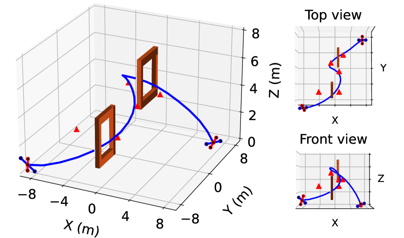
(a) New initial condition 1. Generalization of the polynomial cost learned in Fig. 13(e).

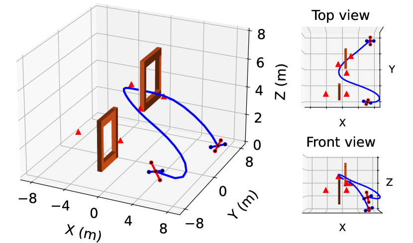
(b) New initial condition 2. Generalization of the polynomial cost learned in Fig. 13(e).

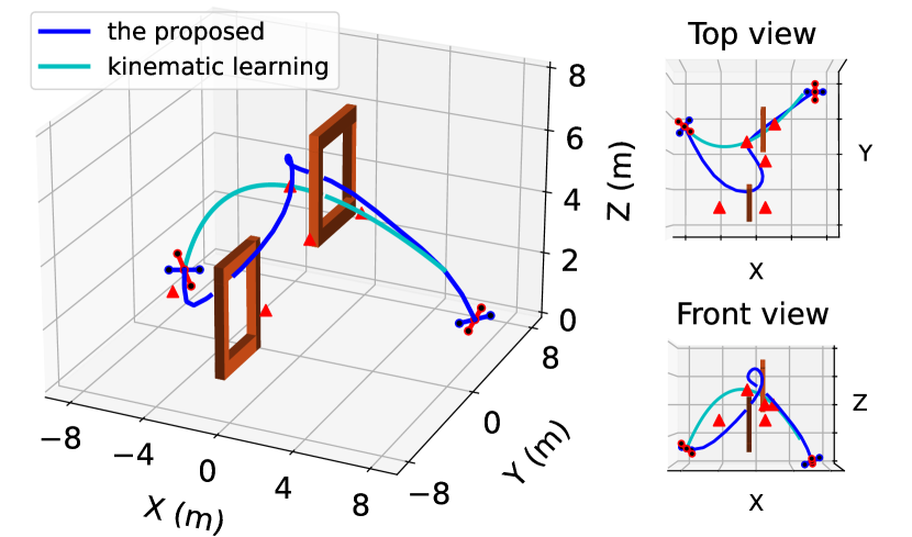
(c) New initial condition 3. Comparing with generalization of kinematic learning [41]

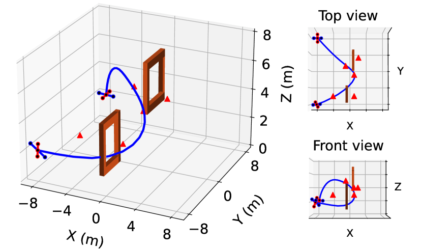
(d) New landing goal. Generalization of the polynomial cost learned in Fig. 13(e).

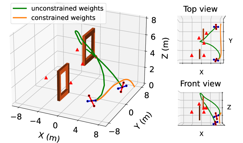
(e) New initial condition 2. Generalization of distance-to-obstacle cost learned in Fig. 13(f).

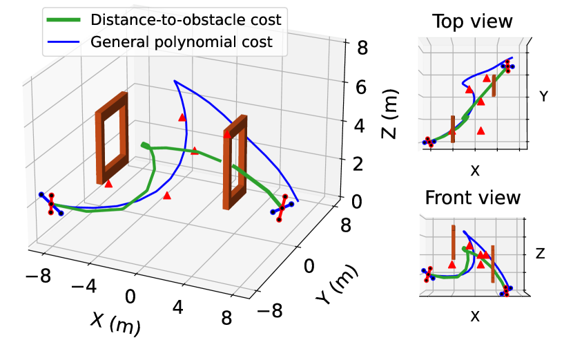
(f) New placement of obstacles. Generalization comparison between the polynomial cost (38a) and distance-to-obstacle cost (40).

Figure 14: Generalization test of the cost functions learned in Fig. 13. (a)-(c) are the generalized motion of the polynomial cost function (learned in Fig. 13(e)) given different new initial conditions. In (c), we also compare with the generalized motion of the kinematic learning method [41] (discussed in Section V-E1). (d) shows the generalized motion of the polynomial cost function (learned in Fig. 13(e)) given a new landing goal. (e) is the generalized motion of the distance-to-obstacle cost function (learned in Fig. 13(f)) given new initial condition 2; here, green and orange colors correspond to the unconstrained and constrained weights subcases, respectively. (f) is the generalization of the polynomial cost function (learned in Fig. 13(e)) and the distance-to-obstacle cost function (learned in Fig. 13(f)) given new placement of obstacles. All quantitative measures are in Table VI.

VI-C Generalization of Learned Cost Functions

In this session, we will test the generalization of the cost functions learned in the previous session. We will set the quadrotor with a new initial condition, a new landing goal, and new placement of obstacles. Given these new conditions, we use the learned cost and time-warping functions to plan the motion of the quadrotor, respectively. We check if the motion plan can successfully achieve the task goal: flying through the gates and landing near the goal position. Quantitatively, we evaluate the generalization performance by calculating the averaged distance between the generalized motion and keyframes and the averaged distance between the generalized motion and the centers of obstacles (gates).

VI-C1 New Initial Conditions

In Fig. 14(a)-Fig. 14(c), we test the generalization of the cost function learned in Fig. 13(d) to new initial conditions (the landing position is the same as the one in the learning stage in the previous session). Here, we use the following new initial conditions, as also visualized in Fig. 14(a)-Fig. 14(c), respectively,

New initial condition 1: position $\boldsymbol{r}_{I}(0){=}[{-}8,{-}10,1]^{\mkern-1.5mu\mathsf{T}}$, attitude quaternion $\boldsymbol{q}_{B/I}(0){=}[0.88,-0.42,0.19,0.14]^{\mkern-1.5mu\mathsf{T}}$, velocity $\boldsymbol{v}_{I}(0){=}[15,0,0]^{\mkern-1.5mu\mathsf{T}}$, and angular velocity $\boldsymbol{\omega}_{B}(0){=}[0,0,0]^{\mkern-1.5mu\mathsf{T}}$.

New initial condition 2: position $\boldsymbol{r}_{I}(0){=}[6,-8,2]^{\mkern-1.5mu\mathsf{T}}$, attitude quaternion $\boldsymbol{q}_{B/I}(0){=}[0.88,-0.45,-0.05,-0.15]^{\mkern-1.5mu\mathsf{T}}$, velocity $\boldsymbol{v}_{I}(0){=}[10,0,0]^{\mkern-1.5mu\mathsf{T}}$, and angular velocity $\boldsymbol{\omega}_{B}(0){=}[0,0,0]^{\mkern-1.5mu\mathsf{T}}$.

New initial condition 3: position $\boldsymbol{r}_{I}(0){=}[-8,5,1]^{\mkern-1.5mu\mathsf{T}}$, attitude quaternion $\boldsymbol{q}_{B/I}(0)=[0.88,0.14,0.14,0.43]^{\mkern-1.5mu\mathsf{T}}$, velocity $\boldsymbol{v}_{I}(0){=}[10,-20,0]^{\mkern-1.5mu\mathsf{T}}$, and angular velocity $\boldsymbol{\omega}_{B}(0){=}[0,0,0]^{\mkern-1.5mu\mathsf{T}}$.

Note that the above new initial conditions are very different from the ones used in learning stage (Fig. 13). For each new initial condition, the generalized motion is shown in Fig. 14(a)-Fig. 14(c), respectively. Fig. 14(c) also plots the generalized motion (cyan color) of the kinematic learning method [41] as a comparison. In Fig. 14(e), we plot the generalized motion from the learned distance-to-obstacle cost function (40) in Fig. 13(f). Here, the green line corresponds to the unconstrained weights subcase and the orange to the constrained weights subcase. The quantitative measures for all generalized motion in Fig. 14 are in Table VI.

TABLE VI: Measure of the generalized motion.

Fig.	Avg. distance to keyframes	Avg. distance to center of gate
14(a)	1.460	0.863
14(b)	1.014	1.187
14(c)	1.715 (the proposed) 3.428 (kinematic learning [41])	1.020 (the proposed) 3.660 (kinematic learning [41])
14(d)	1.841	1.492
14(e)	1.641 (unconstrained weights) 7.580 (constrained weights)	1.423 (unconstrained weights) 7.950 (constrained weights)
14(f)	1.902 (dist.-to-obstacle cost) 1.514 (polynomial cost)	1.617 (dist.-to-obstacle cost) 3.186 (polynomial cost)

• A keyframe’s distance to a trajectory is the distance between this keyframe and its nearest point on the trajectory, and we average the distance over all keyframes.

VI-C2 New Landing Goal

Fig. 14(d) tests the generalization of the cost function learned in Fig. 13(d) to a new landing goal. The initial condition is as follows: position $\boldsymbol{r}_{I}(0){=}[-8,-8,2]^{\mkern-1.5mu\mathsf{T}}$, attitude quaternion $\boldsymbol{q}_{B/I}(0){=}[0.88,-0.42,0.19,0.14]^{\mkern-1.5mu\mathsf{T}}$, velocity $\boldsymbol{v}_{I}(0){=}[15,5,-2]^{\mkern-1.5mu\mathsf{T}}$, and angular velocity $\boldsymbol{\omega}_{B}(0){=}[0,0,0]^{\mkern-1.5mu\mathsf{T}}$. We set the new landing goal to $\boldsymbol{r}_{I}^{\text{g}}=[-8,8,2]^{\mkern-1.5mu\mathsf{T}}$ and $\boldsymbol{q}_{B/I}^{\text{g}}=[0.97,0,0,0.25]^{\mkern-1.5mu\mathsf{T}}$. The quantitative measure for the generalized motion is in Table VI.

VI-C3 New Placement of Obstacles

Fig. 14(f) tests the generalization of the learned cost functions under new placement of obstacles. We change the positions of two gates and then use the learned cost functions to generate new motion in the new environment. The initial condition is the same as the one in Fig. 14(d) and the landing goal as that in Fig. 14(a). Fig. 14(f) shows the generalized motion of the distance-to-obstacle cost function (40) (unconstrained weights, learned in Fig. 13(f)) and the polynomial cost function (38a) (learned in Fig. 13(e)). Note that in the generalization of the distance-to-obstacle cost (40), $o_{i}$ is set as the obstacle’s new location. The quantitative measure for the generalized motion is in Table VI.

VI-C4 Result Analysis

With the new initial conditions and new landing goal, Fig. 14(a)- 14(d) show that the generalized motion can still follow the keyframes, pass through the gates, and land near the goal. Fig. 14(c) also shows that the generalization of the kinematic learning [41] fails to fly through both gates. As discussed in Section V-E1, since [41] focuses on learning a low-level kinematic representation, it has limited generalizability particularly when the new conditions are very different from ones in learning. In contrast, a learned cost function can be shared across different motion conditions. Thus, learning cost functions shows better generalizability. Fig. 14(e) also shows that the generalization of the distance-to-obstacle cost function (40) (unconstrained weights) is comparable to that in Fig. 14(b).

The special attention should be paid to Fig. 14(b) and Fig. 14(e) (unconstrained weights), where the quadrotor seems to have ignored the first two keyframes (and hence the left gate). This could be explained by Bellman’s principle of optimality [58]. Specifically, the motion in Fig. 14(b) can be interpreted as the final segment of the ‘complete’ trajectory in Fig. 13(e), i.e., it can be viewed as the solution to a sub-problem, for which the initial condition starts from a middle point of a ‘complete’ trajectory and minimizes the remaining cost-to-go. In other words, if a complete trajectory from the initial start to a goal is optimal with respect to a cost function, the sub-trajectory of this complete trajectory from any middle point to the goal is also optimal with respect to the same cost function. Thus, the quadrotor motion in Fig. 14(b) and Fig. 14(e) is continuing to finish the rest optimal motion instead of flying back to pass through the first gate.

Fig. 14(f) shows the generalization of the learned distance-to-obstacle cost function (40) versus that of the learned generic polynomial cost function (38a) in a varying environment. With Fig. 14(f) and Table VI, one can conclude that the polynomial cost function generalizes poorly to new placement of obstacles, compared to the distance-to-obstacle cost function. Specifically, the generalized motion of the learned polynomial cost function still tries to follow the original keyframes instead of going through the new gates: its distance to the keyframes is $1.514$ versus the distance-to-obstacle cost function’s $1.902$, while its distance to the centers of gates is $3.186$ versus the distance-to-obstacle cost’s $1.617$. This is understandable because the learned polynomial cost function only ‘remembers’ the representation of the keyframes in the original environment and is unaware of the obstacle changes in the new environment. On the contrary, the distance-to-obstacle cost function (40) is defined on the locations of obstacles, and can be updated with the new locations of obstacles. Hence, in the new environment in Fig. 14(f), the generalized motion of the distance-to-obstacle cost tries to go through the new gates. As indicated in Table VI, the generalization of the distance-to-obstacle cost function has a smaller distance ($1.617$) to the new gates than the polynomial cost does ($3.186$). This can also be visualized in Fig. 14(f), where the motion of the distance-to-obstacle cost is attempting to reach the left gate (although it is not successfully passing through it). The above results suggest that an environment-dependent formulation of cost functions, such as a cost function that is defined on both robot state and environment features, could generalize better in a varying environment. But one also needs to note that such a formulation additionally requires the knowledge/model of the environment features. More discussion of the cost formulations is given in Section VII-B.

In summary of all the above experiments and analyses, we conclude that (i) the proposed method can learn a cost function from a small number of keyframes; (ii) the learned cost function shows good generalization to unseen motion conditions; and (iii) to generalize to varying environments, an environment-informed formulation of cost functions would be needed, such as the cost function formulation which depends on both robot’s state and environment features.

VII Discussion

This section further provides discussion on some aspects of the proposed method.

VII-A Why Do Keyframes Suffice?

We provide one explanation for why sparse keyframes can suffice to recover a cost function. Consider problem (16). For trajectory $\boldsymbol{\xi}_{\boldsymbol{\theta}}$ produced by optimal control system (12), since we are only interested in the trajectory points $\boldsymbol{\xi}_{\boldsymbol{\theta}}{(\tau_{i})}$ at the time stamps $\tau_{i}$ ($1\leq i\leq N$), we discretize the optimal control system at these time steps, yielding [50]

dynamics: $$\,\,\,\boldsymbol{x}_{i+1}={\boldsymbol{\bar{f}}}(\boldsymbol{x}_{i},\bar{\boldsymbol{u}}_{i},\boldsymbol{\theta}),\quad\boldsymbol{x}_{0}=\boldsymbol{x}(0),$$ (41a)

objective: $$\,\,\,J(\boldsymbol{\theta})=\sum_{i=0}^{N-1}\bar{c}(\boldsymbol{x}_{i},\bar{\boldsymbol{u}}_{i},\boldsymbol{{\theta}})+\bar{h}(\boldsymbol{x}_{N},\bar{\boldsymbol{u}}_{N},\boldsymbol{\theta}),$$ (41b)

where we denote $\boldsymbol{x}_{i}=\boldsymbol{x}(\tau_{i})$, and discrete-time ${\boldsymbol{\bar{f}}}$ satisfies

$$\boldsymbol{x}_{i+1} ={\boldsymbol{\bar{f}}}(\boldsymbol{x}_{i},\bar{\boldsymbol{u}}_{i},\boldsymbol{\theta})=\boldsymbol{x}_{i}+\int_{\tau_{i}}^{\tau_{i+1}}v_{\boldsymbol{\beta}}(\tau)\boldsymbol{f}(\boldsymbol{x}(\tau),\boldsymbol{u}(\tau))d\tau,$$

and the discrete version of the cost function satisfies

$$\bar{c}(\boldsymbol{x}_{i},\bar{\boldsymbol{u}}_{i},\boldsymbol{\theta}) =\int_{\tau_{i}}^{\tau_{i+1}}v_{\boldsymbol{\beta}}(\tau)c_{\boldsymbol{p}}(\boldsymbol{x}(\tau),\boldsymbol{u}(\tau))d\tau,$$

$$\bar{h}(\boldsymbol{x}_{N},\bar{\boldsymbol{u}}_{N},\boldsymbol{\theta}) =\int_{\tau_{N}}^{T}v_{\boldsymbol{\beta}}(\tau)c_{\boldsymbol{p}}(\boldsymbol{x}(\tau),\boldsymbol{u}(\tau))d\tau+h_{\boldsymbol{p}}(\boldsymbol{x}(T)).$$

Here, the new input $\bar{\boldsymbol{u}}_{i}\in\mathbb{R}^{d}$ in $\bar{\boldsymbol{f}}$ may not necessarily have the same dimension as $\boldsymbol{u}(\tau)\in\mathbb{R}^{n}$ in the original $\boldsymbol{f}$, e.g., $\bar{\boldsymbol{u}}_{i}$ contains all possible controls over time range $[\tau_{i},\tau_{i+1}]$ [50]. The solution $\{{\boldsymbol{x}_{0:N}},{\bar{\boldsymbol{u}}_{0:N}}\}$ to the discrete-time optimal control system (41) satisfies the KKT conditions:

$$\boldsymbol{x}_{i+1} =\bar{\boldsymbol{f}}(\boldsymbol{x}_{i},\bar{\boldsymbol{u}}_{i},\boldsymbol{\theta}),\quad i=0,\cdots N-1,$$ (42)

$$\boldsymbol{\lambda}_{i} =\frac{\partial\bar{c}}{\partial\boldsymbol{x}_{i}}+\frac{\partial\bar{\boldsymbol{f}}^{\mkern-1.5mu\mathsf{T}}}{\partial\boldsymbol{x}_{i}}\boldsymbol{\lambda}_{i+1}, \quad i=1,\cdots N-1,$$

$$\boldsymbol{0} =\frac{\partial\bar{c}}{\partial\bar{\boldsymbol{u}}_{i}}+\frac{\partial\bar{\boldsymbol{f}}^{\mkern-1.5mu\mathsf{T}}}{\partial\bar{\boldsymbol{u}}_{i}}\boldsymbol{\lambda}_{i+1}, \quad i=0,\cdots N-1,$$

$$\boldsymbol{\lambda}_{N} =\frac{\partial\bar{h}}{\partial\boldsymbol{x}_{N}},\quad\frac{\partial\bar{h}}{\partial\bar{\boldsymbol{u}}_{N}}=\boldsymbol{0} i=N.$$

The output of the discrete-time system (41) can be overloaded by $\boldsymbol{y}(\tau_{i})=\boldsymbol{g}(\boldsymbol{x}_{i},\bar{\boldsymbol{u}}_{i})$. To simplify analysis, we assume that keyframes $\mathcal{D}$ are realizable by a $\boldsymbol{\theta}$. Then,

$$\boldsymbol{y}^{*}({\tau}_{i})=\boldsymbol{g}(\boldsymbol{x}_{i},\bar{\boldsymbol{u}}_{i}).$$ (43)

Given the keyframes $\mathcal{D}$ in (5), recovering a cost function can be viewed as a problem of solving a set of non-linear equations in (42) and (43), where unknowns are $\{\boldsymbol{x}_{1:N},\bar{\boldsymbol{u}}_{0:N},\boldsymbol{\lambda}_{1:N},\boldsymbol{\theta}\}\in\mathbb{R}^{2Nn+(N+1)d+(r+s)}$, and the total number of constraints (equations) are $2Nn+(N+1)d+No$. Here, $(r+s)$ is the dimension of $\boldsymbol{\theta}$ and $o$ is the dimension of $\boldsymbol{y}$. A necessary condition to uniquely determine $\{\boldsymbol{x}_{1:N},\bar{\boldsymbol{u}}_{0:N},\boldsymbol{\lambda}_{1:N},\boldsymbol{\theta}\}$ requires the number of constraints to be no less than the number of unknowns, yielding

$$N\geq\frac{r+s}{o}.$$ (44)

On the other hand, if (44) is not fulfilled or given $\mathcal{D}$ is less informative, the unknowns then cannot be uniquely determined, which means that there might exist multiple $\boldsymbol{\theta}$s such that all resulting trajectories pass the same sparse keyframes. This case has been shown in Section V-A (Fig. 4).

Note that the above discussion uses a perspective different from the development of this paper. It should be noted that the above explanation fails to explain the case where the given keyframes are not realizable: $\min_{\boldsymbol{\theta}}L(\boldsymbol{\xi}_{\boldsymbol{\theta}},\mathcal{D})>0$, e.g., sub-optimal data as in Section V-B. We leave its further exploration as one future direction of this work.

VII-B Cost Function Formulation

In general, there are two types of cost function formulations, as discussed below.

VII-B1 Cost Depending Purely on Robot States

The first type of cost function formulation can be written as $c_{\boldsymbol{p}}(\boldsymbol{x},\boldsymbol{u})$, which only depends on robot state and input $(\boldsymbol{x},\boldsymbol{u})$. The polynomial cost function (38a) in Section VI belongs to this type. This formulation type can generalize well to different motion conditions, e.g., new initial condition and new goals, as shown in Fig. 14(a) - Fig. 14(e). However, it cannot generalize to varying environments as in Fig. 14(f), as the environment information is not explicitly captured in this cost formulation.

VII-B2 Cost Depending on Robot States and Environment Features

The second type of cost formulations can be written as $c_{\boldsymbol{p}}(\boldsymbol{x},\boldsymbol{u},\boldsymbol{o})$, which depends on both the robot state-input $(\boldsymbol{x},\boldsymbol{u})$ and the environment features $\boldsymbol{o}$. Here, $\boldsymbol{o}$ should be given for the environment where the robot is trained. Demonstrations from different environments can also be used as the training data. The cost functions in (29) and (40) belong to this type. One advantage of this formulation is that it has the ability to generalize to a new environment given its environment features $\boldsymbol{o}$. Section VI-C3 has shown such an advantage by comparing with the first type of cost formulation. At the same time, one should note that the second type of cost formulation requires the knowledge of environment features $\boldsymbol{o}$, which may need additional modeling effort.

VII-B3 Running Cost and Final Cost

The cost function in (2) includes two terms: a running cost term $c(\cdot)$ and a final cost term $h(\cdot)$. If no knowledge about the task goal is available, one can use a (deep) neural network to represent both costs, as shown in Section V-D. Since a neural cost function is usually goal-blind, the training data needs to include a keyframe at the goal. If the task goal is known, such as in motion planning in Section VI, the final cost $h(\cdot)$ can be set to the distance-to-goal cost, and the running cost $c(\cdot)$ is to be tuned. Tuning a running cost will determine how the robot moves to the goal. This has been shown in Section VI.

VII-B4 Limitation

We should note that whatever a cost formulation is, the proposed method requires all functions to be differentiable. This can be a limitation of the proposed method, compared to some existing feature-based IRL methods such as max-entropy IRL [15], which permits non-differentiable features. How to extend the proposed method to non-differentiable systems is a topic for our future work.

VII-C Convergence and Numerical Integration Error

VII-C1 Algorithm Convergence

The proposed Continuous PDP solves a bi-level optimization problem (16) using gradient descent. It treats the trajectory $\boldsymbol{\xi}_{\boldsymbol{\theta}}$ of the inner-level optimal control system simply as an ‘implicit’ differentiable function of the system parameter $\boldsymbol{\theta}$. Generally, bi-level optimization is known to be strongly NP-hard [59, 60]. Under certain assumptions, one can prove that the gradient-descent method can converge to a stationary point [61]. With further assumptions on the outer-level and inner-level problems, such as convexity and smoothness, [62] shows that the gradient-descent method could converge to the global solution. However, in our case, the requirement of convexity is too restricted to optimal control systems (12). As a future direction of this work, we will try to explore the milder conditions for its convergence.

VII-C2 Numerical Integration Error

Another issue that might arise is the numerical integration error in solving the gradient of the inner-level trajectory using Lemma 1, as it requires integrating several ODEs in both backward and forward passes. However, our previous experimental experience shows that due to the side effect of a time-warping function, numerical integration error/stability can be potentially mitigated. A similar process has also been successfully used in some optimal control software such as [50].

A side effect of using a time-warping function $t=w(\tau)$ is that one can scale a long-horizon integration into a smaller horizon problem by time-warping transformation, then re-scale the solution back after integration (some refinement can be done afterwards). For example, $\int_{0}^{t_{f}}c(\boldsymbol{x}(t),\boldsymbol{u}(t))dt$ in (2) over $[0,t_{f}]$ can be transformed to $\int_{0}^{T}\frac{dw(\tau)}{d\tau}c(\boldsymbol{x}(\tau),\boldsymbol{u}(\tau))d\tau$ in (12b) over the new horizon $[0,T]$, using the time-warping function $t_{f}=w(T)$. In our problem of interest, since $T$ is given, one can manually pick a relatively small horizon $T<t_{f}$ and a small integration step size to mitigate the error of numerical integration. In our previous experiments, we set the keyframe horizon as $T=1$ for good numerical integration accuracy. This time-warping trick has been successfully adopted by some optimal control software such as [50] for numerical stability. One important caveat is that by using the time-warping transformation $t=w(\tau)$, as shown from (2) to (12b), we have changed the original integrand $c(\boldsymbol{x}(t),\boldsymbol{u}(t))$ to the new $\frac{dw(\tau)}{d\tau}c(\boldsymbol{x}(\tau),\boldsymbol{u}(\tau))$. Hence, if one wants to significantly decrease the horizon, i.e., $T\ll t_{f}$, $\frac{dw(\tau)}{d\tau}$ would be very large, which may increase the stiffness of $\frac{dw(\tau)}{d\tau}c(\boldsymbol{x}(\tau),\boldsymbol{u}(\tau))$, causing numerical instability. Although we have rarely encountered such numerical issues in our previous experiments with $T=1$s, one might be cautious when handling stiff ODEs/systems.

VII-D Model-free versus Model-based

The formulation in this paper assumes robot dynamics to be known. We would point out that the proposed Continuous PDP is also able to solve model-free IOC/IRL, i.e., jointly learning a dynamics model and a cost function from keyframes. To do that, one needs to replace the known dynamics (1) with a parameterized dynamics model, which should be differentiable. The Continuous PDP can update all parameters (including both dynamics and objective parameters) using gradient descent. We refer the reviewer to our previous work Pontryagin Differentiable Programming (PDP) [34, 46] (discrete-time) for the model-free IOC/IRL formulation and experiments.

In fact, after the problem reformulation in Section III.B, as shown in (12a), the parameter of the time-warping function has been absorbed into the dynamics model and becomes the unknown parameter in the dynamics. Thus, the Continuous PDP has already shown its ability to jointly update the parameters in both the dynamics model and cost function.

VIII Conclusions

This paper proposes the method of Continuous Pontryagin Differentiable Programming (Continuous PDP) to enable a robot to learn an objective function from a small set of demonstrated keyframes. As the given time stamps of the keyframes may not be achievable in the robot’s actual execution, the Continuous PDP jointly finds an objective function and a time-warping function such that the robot’s final motion attains the minimal discrepancy loss to the keyframes. The Continuous PDP minimizes the discrepancy loss using projected gradient descent, by efficiently computing the gradient of the optimal trajectory with respect to the tunable function parameters in the system. The efficacy and capability of the Continuous PDP are demonstrated in robot arm and 6-DoF quadrotor planning tasks.

[Proof of Lemma 1] We consider the equation of Differential Pontryagin’s Maximum Principle in (22). Suppose that ${H_{uu}(\tau)}$ in (23c) is invertible for all $0\leq\tau\leq T$. We can solve $\frac{\partial\boldsymbol{u}_{\boldsymbol{\theta}}}{\partial\boldsymbol{\theta}}$ from (22c):

$$\frac{\partial\boldsymbol{u}_{\boldsymbol{\theta}}}{\partial\boldsymbol{\theta}}={-}H_{uu}^{-1}(\tau)\Big{(}H_{ux}(\tau)\frac{\partial\boldsymbol{x}_{\boldsymbol{\theta}}}{\partial\boldsymbol{\theta}}{+}{G}(\tau)^{\mkern-1.5mu\mathsf{T}}\frac{\partial\boldsymbol{\lambda}_{\boldsymbol{\theta}}}{\partial\boldsymbol{\theta}}{+}H_{ue}(\tau)\Big{)}.$$ (45)

Substituting (45) into both (22a) and (22b) and combining the definition of matrices in (25), we have

$$\frac{d}{d\tau}(\frac{\partial\boldsymbol{x}_{\boldsymbol{\theta}}}{\partial\boldsymbol{\theta}}) =A(\tau)\frac{\partial\boldsymbol{x}_{\boldsymbol{\theta}}}{\partial\boldsymbol{\theta}}-R(\tau)\frac{\partial\boldsymbol{\lambda}_{\boldsymbol{\theta}}}{\partial\boldsymbol{\theta}}+M(\tau),$$ (46a)

$$-\frac{d}{d\tau}(\frac{\partial\boldsymbol{\lambda}_{\boldsymbol{\theta}}}{\partial\boldsymbol{\theta}}) =Q(\tau)\frac{\partial\boldsymbol{x}_{\boldsymbol{\theta}}}{\partial\boldsymbol{\theta}}+A(\tau)^{\prime}\frac{\partial\boldsymbol{\lambda}_{\boldsymbol{\theta}}}{\partial\boldsymbol{\theta}}+N(\tau).$$ (46b)

Motivated by (22d), we assume

$$\frac{\partial\boldsymbol{\lambda}_{\boldsymbol{\theta}}}{\partial\boldsymbol{\theta}}=P(\tau)\frac{\partial\boldsymbol{x}_{\boldsymbol{\theta}}}{\partial\boldsymbol{\theta}}+W(\tau),$$ (47)

with $P(\tau)\in\mathbb{R}^{n\times n}$ and $W(\tau)\in\mathbb{R}^{n\times(s+r)}$, $0\leq\tau\leq T$, are two time-varying matrices. Of course, the above (47) holds for $\tau=T$ because of (22d), if

$$P(\tau)=H_{xx}(T)\quad\text{and}\quad W(\tau)=H_{xe}(T).$$ (48)

Substituting (47) to (46a) and (46b), respectively, to eliminate $\frac{\partial\boldsymbol{x}_{\boldsymbol{\theta}}}{\partial\boldsymbol{\theta}}$, we obtain the following

$$\frac{d}{d\tau}(\frac{\partial\boldsymbol{x}_{\boldsymbol{\theta}}}{\partial\boldsymbol{\theta}}) {=}(A-RP)\frac{\partial\boldsymbol{x}_{\boldsymbol{\theta}}}{\partial\boldsymbol{\theta}}+(-RW+M),$$ (49a)

$${-}\dot{P}\frac{d}{d\tau}(\frac{\partial\boldsymbol{x}_{\boldsymbol{\theta}}}{\partial\boldsymbol{\theta}}) {=}(Q{+}\dot{P}{+}A^{\mkern-1.5mu\mathsf{T}}P)\frac{\partial\boldsymbol{x}_{\boldsymbol{\theta}}}{\partial\boldsymbol{\theta}}{+}(A^{\prime}W{+}N{+}\dot{W}),$$ (49b)

where $\dot{P}=\frac{dP(\tau)}{d\tau}$, $\dot{W}=\frac{dW(\tau)}{d\tau}$, and we here have suppressed the dependence of $\tau$ for all time-varying matrices. By multiplying $(-\dot{P})$ on both sides of (49a), and equaling the left sides of (49a) and (49b), we have

$$(-PA+PRP)\frac{\partial\boldsymbol{x}_{\boldsymbol{\theta}}}{\partial\boldsymbol{\theta}}+(PRW-PM)$$

$$= (Q+\dot{P}+A^{\mkern-1.5mu\mathsf{T}}P)\frac{\partial\boldsymbol{x}_{\boldsymbol{\theta}}}{\partial\boldsymbol{\theta}}+(A^{\mkern-1.5mu\mathsf{T}}W+N+\dot{W}).$$ (50)

The above equation holds if

$$-PA+PRP =Q+\dot{P}+A^{\mkern-1.5mu\mathsf{T}}P,$$ (51a)

$$PRW-PM =A^{\mkern-1.5mu\mathsf{T}}W+N+\dot{W},$$ (51b)

which directly are (24). Substituting (47) into (45) yields (27a), and (27b) directly results from (22a). This completes the proof. ∎

Wanxin Jin is a postdoctoral researcher in the GRASP Laboratory at the University of Pennsylvania. He received the Ph.D. degree in Autonomy and Control at Purdue University in 2021. From 2016 to 2017, he was a Research Assistant at Technical University Munich, Germany. Wanxin’s research interests include robotics, control, machine learning, and optimization, with emphasis on learning, planning, and control of robots as they interact with the world and humans.

Todd D. Murphey received his B.S. degree in mathematics from the University of Arizona and the Ph.D. degree in Control and Dynamical Systems from the California Institute of Technology. He is a Professor of Mechanical Engineering at Northwestern University. His laboratory is part of the Center for Robotics and Biosystems, and his research interests include robotics, control, machine learning in physical systems, and computational neuroscience.

Dana Kulić conducts research in robotics and human-robot interaction (HRI), and develops autonomous systems that can operate in concert with humans, using natural and intuitive interaction strategies while learning from user feedback to improve and individualize operation over long-term use. Dana Kulić received the combined B. A. Sc. and M. Eng. degree in electro-mechanical engineering, and the Ph. D. degree in mechanical engineering from the University of British Columbia, Canada, in 1998 and 2005, respectively. From 2006 to 2009, Dr. Kulić was a JSPS Post-doctoral Fellow and a Project Assistant Professor at the Nakamura-Yamane Laboratory at the University of Tokyo, Japan. In 2009, Dr. Kulić established the Adaptive System Laboratory at the University of Waterloo, Canada, conducting research in human robot interaction, human motion analysis for rehabilitation and humanoid robotics. Since 2019, Dr. Kulić is a professor and director of Monash Robotics at Monash University, Australia. In 2020, Dr. Kulić was awarded the ARC Future Fellowship. Her research interests include robot learning, humanoid robots, human-robot interaction and mechatronics.

Neta Ezer is the Northrop Grumman Corporate Director of Strategic Planning. Dr. Ezer previously served as Technical Fellow and Chief Technologist for Human-Machine Teaming in Northrop Grumman Mission Systems and as an Artificial Intelligence (AI) Architect for the Northrop Grumman AI Campaign. Prior to Northrop Grumman, Dr. Ezer was a Senior Human Engineering Researcher at the Futron Corporation, working on NASA Orion, International Space Station and human-robot interaction research. She served as Assistant Professor of Industrial Design at the Georgia Institute of Technology. Dr. Ezer has over 15 years of experience in human factors, user experience and AI, with over 40 published papers and proceedings in these areas. Dr. Ezer holds a B.S. in Industrial Design and M.S. and PhD degrees in Engineering Psychology from the Georgia Institute of Technology.

Shaoshuai Mou is an Associate Professor in the School of Aeronautics and Astronautics at Purdue University. Before joining Purdue, he received a Ph.D. in Electrical Engineering at Yale University in 2014 and worked as a postdoc researcher at MIT for a year after that. His research interests include multi-agent system, control and learning, robotics control, human-robot teaming, resilient autonomy, and also experimental research involving autonomous air and ground vehicles. Dr. Mou co-directs Purdue University’s Center for Innovation in Control, Optimization and Networks (ICON), which aims to integrate classical theories in control/optimization/networks with recent advances in machine learning/AI/data science to address fundamental challenges in autonomous and connected systems.

References

- [1] H. Ravichandar, A. S. Polydoros, S. Chernova, and A. Billard, “Recent advances in robot learning from demonstration,” Annual Review of Control, Robotics, and Autonomous Systems, vol. 3, 2020.
- [2] M. Deniša, A. Gams, A. Ude, and T. Petrič, “Learning compliant movement primitives through demonstration and statistical generalization,” IEEE/ASME transactions on mechatronics, vol. 21, no. 5, pp. 2581–2594, 2015.
- [3] C. Moro, G. Nejat, and A. Mihailidis, “Learning and personalizing socially assistive robot behaviors to aid with activities of daily living,” ACM Transactions on Human-Robot Interaction, vol. 7, no. 2, pp. 1–25, 2018.
- [4] M. Kuderer, S. Gulati, and W. Burgard, “Learning driving styles for autonomous vehicles from demonstration,” in IEEE International Conference on Robotics and Automation, 2015, pp. 2641–2646.
- [5] D. A. Pomerleau, “Efficient training of artificial neural networks for autonomous navigation,” Neural computation, vol. 3, no. 1, pp. 88–97, 1991.
- [6] P. Englert, A. Paraschos, M. P. Deisenroth, and J. Peters, “Probabilistic model-based imitation learning,” Adaptive Behavior, vol. 21, no. 5, pp. 388–403, 2013.
- [7] S. Calinon, F. Guenter, and A. Billard, “On learning, representing, and generalizing a task in a humanoid robot,” IEEE Transactions on Systems, Man, and Cybernetics, vol. 37, no. 2, pp. 286–298, 2007.
- [8] R. Rahmatizadeh, P. Abolghasemi, L. Bölöni, and S. Levine, “Vision-based multi-task manipulation for inexpensive robots using end-to-end learning from demonstration,” in IEEE International Conference on Robotics and Automation, 2018, pp. 3758–3765.
- [9] F. Torabi, G. Warnell, and P. Stone, “Behavioral cloning from observation,” in International Joint Conference on Artificial Intelligence, 2018, pp. 4950–4957.
- [10] P. Abbeel and A. Y. Ng, “Apprenticeship learning via inverse reinforcement learning,” in International Conference on Machine Learning, 2004, pp. 1–8.
- [11] A. Y. Ng, S. J. Russell et al., “Algorithms for inverse reinforcement learning.” in International Conference of Machine Learning, vol. 1, 2000, p. 2.
- [12] P. Moylan and B. Anderson, “Nonlinear regulator theory and an inverse optimal control problem,” IEEE Transactions on Automatic Control, vol. 18, no. 5, pp. 460–465, 1973.
- [13] J. MacGlashan and M. L. Littman, “Between imitation and intention learning,” in International Joint Conference on Artificial Intelligence, 2015.
- [14] N. D. Ratliff, J. A. Bagnell, and M. A. Zinkevich, “Maximum margin planning,” in International Conference on Machine Learning, 2006, pp. 729–736.
- [15] B. D. Ziebart, A. L. Maas, J. A. Bagnell, and A. K. Dey, “Maximum entropy inverse reinforcement learning.” in Association for the Advancement of Artificial Intelligence, vol. 8, 2008, pp. 1433–1438.
- [16] K. Mombaur, A. Truong, and J.-P. Laumond, “From human to humanoid locomotion—an inverse optimal control approach,” Autonomous Robots, vol. 28, no. 3, pp. 369–383, 2010.
- [17] A. Keshavarz, Y. Wang, and S. Boyd, “Imputing a convex objective function,” in IEEE International Symposium on Intelligent Control. IEEE, 2011, pp. 613–619.
- [18] A.-S. Puydupin-Jamin, M. Johnson, and T. Bretl, “A convex approach to inverse optimal control and its application to modeling human locomotion,” in International Conference on Robotics and Automation, 2012, pp. 531–536.
- [19] P. Englert, N. A. Vien, and M. Toussaint, “Inverse kkt: Learning cost functions of manipulation tasks from demonstrations,” International Journal of Robotics Research, vol. 36, no. 13-14, pp. 1474–1488, 2017.
- [20] P. Kingston and M. Egerstedt, “Time and output warping of control systems: Comparing and imitating motions,” Automatica, vol. 47, no. 8, pp. 1580–1588.
- [21] T. Osa, J. Pajarinen, G. Neumann, J. A. Bagnell, P. Abbeel, J. Peters et al., “An algorithmic perspective on imitation learning,” Foundations and Trends in Robotics, vol. 7, no. 1-2, pp. 1–179, 2018.
- [22] A. Doerr, N. D. Ratliff, J. Bohg, M. Toussaint, and S. Schaal, “Direct loss minimization inverse optimal control.” in Robotics: Science and Systems, 2015.
- [23] W. Jin, D. Kulić, S. Mou, and S. Hirche, “Inverse optimal control from incomplete trajectory observations,” International Journal of Robotics Research, vol. 40, no. 6-7, pp. 848–865, 2021.
- [24] W. Jin, D. Kulić, J. F.-S. Lin, S. Mou, and S. Hirche, “Inverse optimal control for multiphase cost functions,” IEEE Transactions on Robotics, vol. 35, no. 6, pp. 1387–1398, 2019.
- [25] H. W. Kuhn and A. W. Tucker, “Nonlinear programming,” in Traces and Emergence of Nonlinear Programming. Springer, 2014, pp. 247–258.
- [26] L. S. Pontryagin, V. G. Boltyanskiy, R. V. Gamkrelidze, and E. F. Mishchenko, The Mathematical Theory of Optimal Processes. John Wiley & Sons, Inc., 1962.
- [27] W. Jin and S. Mou, “Distributed inverse optimal control,” Automatica, vol. 129, p. 109658, 2021.
- [28] K. Mombaur, A.-H. Olivier, and A. Crétual, “Forward and inverse optimal control of bipedal running,” in Modeling, simulation and optimization of bipedal walking. Springer, 2013, pp. 165–179.
- [29] M. J. Powell, “The bobyqa algorithm for bound constrained optimization without derivatives,” Cambridge NA Report, University of Cambridge, Cambridge, pp. 26–46, 2009.
- [30] L. M. Rios and N. V. Sahinidis, “Derivative-free optimization: a review of algorithms and comparison of software implementations,” Journal of Global Optimization, vol. 56, no. 3, pp. 1247–1293, 2013.
- [31] K. Hatz, J. P. Schloder, and H. G. Bock, “Estimating parameters in optimal control problems,” SIAM Journal on Scientific Computing, vol. 34, no. 3, pp. A1707–A1728, 2012.
- [32] N. Das, S. Bechtle, T. Davchev, D. Jayaraman, A. Rai, and F. Meier, “Model-based inverse reinforcement learning from visual demonstrations,” in Conference on Robotic Learning, pp. 1930–1942.
- [33] M. Abadi, P. Barham, J. Chen, Z. Chen, A. Davis, J. Dean, M. Devin, S. Ghemawat, G. Irving, M. Isard, M. Kudlur, J. Levenberg, R. Monga, S. Moore, D. G. Murray, B. Steiner, P. Tucker, V. Vasudevan, P. Warden, M. Wicke, Y. Yu, and X. Zheng, “TensorFlow: A system for Large-Scale machine learning,” in 12th USENIX Symposium on Operating Systems Design and Implementation (OSDI 16). USENIX Association, 2016, pp. 265–283.
- [34] W. Jin, Z. Wang, Z. Yang, and S. Mou, “Pontryagin differentiable programming: An end-to-end learning and control framework,” in Advances in Neural Information Processing Systems, 2020.
- [35] B. Amos, I. Jimenez, J. Sacks, B. Boots, and J. Z. Kolter, “Differentiable mpc for end-to-end planning and control,” in Advances in Neural Information Processing Systems, 2018, pp. 8299––8310.
- [36] H. Sakoe and S. Chiba, “Dynamic programming algorithm optimization for spoken word recognition,” IEEE Transactions on Acoustics, Speech, and Signal Processing, vol. 26, no. 1, pp. 43–49, 1978.
- [37] C.-Y. Chang, D.-A. Huang, Y. Sui, L. Fei-Fei, and J. C. Niebles, “D3tw: Discriminative differentiable dynamic time warping for weakly supervised action alignment and segmentation,” in IEEE Conference on Computer Vision and Pattern Recognition, 2019, pp. 3546–3555.
- [38] A. Vakanski, I. Mantegh, A. Irish, and F. Janabi-Sharifi, “Trajectory learning for robot programming by demonstration using hidden markov model and dynamic time warping,” IEEE Transactions on Systems, Man, and Cybernetics, vol. 42, no. 4, pp. 1039–1052, 2012.
- [39] N. Vuković, M. Mitić, and Z. Miljković, “Trajectory learning and reproduction for differential drive mobile robots based on gmm/hmm and dynamic time warping using learning from demonstration framework,” Engineering Applications of Artificial Intelligence, vol. 45, pp. 388–404, 2015.
- [40] Z. Liang, W. Jin, and S. Mou, “An iterative method for inverse optimal control,” in Asian Control Conference, 2022, pp. 959–964.
- [41] B. Akgun, M. Cakmak, K. Jiang, and A. L. Thomaz, “Keyframe-based learning from demonstration,” International Journal of Social Robotics, vol. 4, no. 4, pp. 343–355, 2012.
- [42] B. Akgun, M. Cakmak, J. W. Yoo, and A. L. Thomaz, “Trajectories and keyframes for kinesthetic teaching: A human-robot interaction perspective,” in ACM/IEEE international conference on Human-Robot Interaction, 2012, pp. 391–398.
- [43] A. V. Fiacco, “Sensitivity analysis for nonlinear programming using penalty methods,” Mathematical programming, vol. 10, no. 1, pp. 287–311, 1976.
- [44] A. Levy and R. Rockafellar, “Sensitivity of solutions in nonlinear programs with nonunique multiplier,” Recent Advances in Nonsmooth Optimzation, pp. 215–223.
- [45] S. G. Krantz and H. R. Parks, The implicit function theorem: history, theory, and applications. Springer Science & Business Media, 2012.
- [46] W. Jin, S. Mou, and G. J. Pappas, “Safe pontryagin differentiable programming,” in Advances in Neural Information Processing Systems, 2021.
- [47] W. Li and E. Todorov, “Iterative linear quadratic regulator design for nonlinear biological movement systems,” in International Conference on Informatics in Control, Automation and Robotics, vol. 2, 2004, pp. 222–229.
- [48] D. H. Jacobson and D. Q. Mayne, Differential dynamic programming. Elsevier Publishing Company, 1970, no. 24.
- [49] J. A. E. Andersson, J. Gillis, G. Horn, J. B. Rawlings, and M. Diehl, “CasADi – A software framework for nonlinear optimization and optimal control,” Mathematical Programming Computation, vol. 11, no. 1, pp. 1–36, 2019.
- [50] M. A. Patterson and A. V. Rao, “Gpops-ii: A matlab software for solving multiple-phase optimal control problems using hp-adaptive gaussian quadrature collocation methods and sparse nonlinear programming,” ACM Transactions on Mathematical Software, vol. 41, no. 1, pp. 1–37, 2014.
- [51] C. D. Kolstad and L. S. Lasdon, “Derivative evaluation and computational experience with large bilevel mathematical programs,” Journal of optimization theory and applications, vol. 65, no. 3, pp. 485–499, 1990.
- [52] F. L. Lewis, D. Vrabie, and V. L. Syrmos, Optimal control. John Wiley & Sons, 2012.
- [53] M. W. Spong and M. Vidyasagar, Robot dynamics and control. John Wiley & Sons, 2008.
- [54] C. C. Aggarwal et al., “Neural networks and deep learning,” Springer, vol. 10, pp. 978–3, 2018.
- [55] A. Wächter and L. T. Biegler, “On the implementation of an interior-point filter line-search algorithm for large-scale nonlinear programming,” Mathematical programming, vol. 106, no. 1, pp. 25–57, 2006.
- [56] J. B. Kuipers, Quaternions and rotation sequences. Princeton University Press, 1999, vol. 66.
- [57] T. Lee, M. Leok, and N. H. McClamroch, “Geometric tracking control of a quadrotor uav on se(3),” in IEEE Conference on Decision and Control, 2010, pp. 5420–5425.
- [58] R. Bellman, “Dynamic programming,” Science, vol. 153, no. 3731, pp. 34–37, 1966.
- [59] P. Hansen, B. Jaumard, and G. Savard, “New branch-and-bound rules for linear bilevel programming,” SIAM Journal on scientific and Statistical Computing, vol. 13, no. 5, pp. 1194–1217, 1992.
- [60] A. Sinha, P. Malo, and K. Deb, “A review on bilevel optimization: from classical to evolutionary approaches and applications,” IEEE Transactions on Evolutionary Computation, vol. 22, no. 2, pp. 276–295, 2017.
- [61] K. Ji, J. Yang, and Y. Liang, “Bilevel optimization: Convergence analysis and enhanced design,” in International Conference on Machine Learning, 2021, pp. 4882–4892.
- [62] S. Ghadimi and M. Wang, “Approximation methods for bilevel programming,” arXiv preprint arXiv:1802.02246, 2018.