Reducing Isotropy and Volume to KLS: An $O^{*}(n^{3}\psi^{2})\text{ }$Volume Algorithm

Abstract

We show that the volume of a convex body in $\mathbb{R}^{n}$ in the general membership oracle model can be computed to within relative error $\varepsilon$ using $\widetilde{O}(n^{3}\psi^{2}+n^{3}/\varepsilon^{2})$ oracle queries, where $\psi$ is the KLS constant. With the current bound of $\psi=\widetilde{O}(1)$, this gives an $\widetilde{O}(n^{3}/\varepsilon^{2})$ algorithm, improving on the Lovász-Vempala $\widetilde{O}(n^{4}/\varepsilon^{2})$ algorithm from 2003. The main new ingredient is an $\widetilde{O}(n^{3}\psi^{2})$ algorithm for isotropic transformation, following which we can apply the $\widetilde{O}(n^{3}/\varepsilon^{2})$ volume algorithm of Cousins and Vempala for well-rounded convex bodies. We also give an efficient implementation of the new algorithm for convex polytopes defined by $m$ inequalities in $\mathbb{R}^{n}$: polytope volume can be estimated in time $\widetilde{O}(mn^{c}/\varepsilon^{2})$ where $c<3.2$ depends on the current matrix multiplication exponent and improves on the previous best bound.

1 Introduction

Computing the volume is a fundamental problem from antiquity, playing a central role in the development of fields such as integral calculus, thermodynamics and fluid dynamics. Over the past several decades, numerical estimation of the volumes of high-dimensional bodies that arise in applications has been of great interest. To mention one example from systems biology, volume has been proposed as a promising parameter to distinguish between the metabolic networks of normal and abnormal individuals [10] where the networks are modeled as very high dimensional polytopes.

As an algorithmic problem for convex bodies in $\mathbb{R}^{n}$, volume computation has a four-decade history. Early results by Barány and by Barány and Füredi showed that any deterministic algorithm for the task is doomed to have an exponential complexity, even to approximate the volume to within an exponentially large factor. Then came the stunning breakthrough of Dyer, Frieze, and Kannan showing that with randomization, the problem can be solved in full generality (the membership oracle model) to an arbitrary relative error $\varepsilon$ in time polynomial in $n$ and $1/\varepsilon$. They used the Markov chain Monte Carlo method and reduced the volume problem to sampling uniformly from a sequence of convex bodies, and showed that the sampling itself can be done in polynomial-time. Subsequent progress on the complexity of volume computation has been accompanied by the discovery of several techniques of independent interest, summarized below. The current best complexity of $\widetilde{O}(n^{4}/\epsilon^{2})$ for general convex bodies is achieved by the 2003 algorithm of Lovász and Vempala.

Year/Authors	New ingredients	Steps
1989/Dyer-Frieze-Kannan [8]	Everything	$n^{23}$
1990/Lovász-Simonovits [22]	Better isoperimetry	$n^{16}$
1990/Lovász [21]	Ball walk	$n^{10}$
1991/Applegate-Kannan [3]	Logconcave sampling	$n^{10}$
1990/Dyer-Frieze [7]	Better error analysis	$n^{8}$
1993/Lovász-Simonovits [23]	Localization lemma	$n^{7}$
1997/Kannan-Lovász-Simonovits [14]	Speedy walk, isotropy	$n^{5}$
2003/Lovász-Vempala [24]	Annealing, hit-and-run	$n^{4}$
2015/Cousins-Vempala [5] (well-rounded)	Gaussian Cooling	$n^{3}$

Table 1: The complexity of volume estimation. The complexity of all algorithms has an $\epsilon^{-2}$ factor. Each step uses $\widetilde{O}(n)$ bit of randomness and $\widetilde{O}(n^{2})$ arithmetic operations. The last algorithm is for well-rounded convex bodies.

The main subroutine for volume computation is sampling. Sampling is done by random walks, notably the ball walk and hit-and-run. The rate of convergence of random walks is determined by their conductance. For a Markov chain with state space $\Omega$, transition function $P_{u}(.)$ and stationary density $Q$, the conductance is

$$\phi=\min_{A\subset\Omega:Q(A)\leq\frac{1}{2}}\frac{\int_{u\in A}P_{u}(\Omega\setminus A)\,dQ(u)}{Q(A)}$$

i.e., the minimum conditional escape probability with the stationary density (probability of crossing from a set to its complement starting from the stationary density in the set). The analysis of the ball walk done in [14] shows that the conductance can be bounded in terms of the isoperimetry of the stationary distribution, a purely geometric parameter. For an $n$-dimensional measure $\nu,$ its KLS constant (the isoperimetric or Cheeger constant is the reciprocal) is

$$\frac{1}{\psi_{\nu}}=\inf_{A\subset\mathbb{R}:Q(A)\leq\frac{1}{2}}\frac{\nu_{n-1}(\partial A)}{\nu(A)}$$

where $\partial A$ is the boundary of the set $A$, and $\nu_{n-1}$ is the induced $(n-1)$-dimensional measure. The conductance of the Markov chain reduces to the isoperimetry of its stationary density:

$$\phi\apprge\frac{1}{\psi\cdot n}$$

with $\psi$ being the KLS constant of the stationary density of the Markov chain. This implies a mixing rate of $O(n^{2}\psi^{2})$. Thus, bounding the KLS constant becomes critical, and this consideration originally motivated the KLS conjecture. With many unexpected connections and applications since its formulation, the conjecture has become a central part of asymptotic convex geometry and functional analysis. (A distribution is said to be isotropic if it has zero mean and identity covariance, see Def. 2.2).

Conjecture 1.1 (KLS Conjecture [13]).

The KLS constant of any isotropic logconcave density in any dimension is bounded by an absolute constant. Equivalently, for a logconcave density $q$ with covariance matrix $A$, we have $\psi_{q}\lesssim\left\|A\right\|_{\mathrm{op}}^{1/2}$.

Another equivalent formulation of the conjecture is that for any logconcave density, a halfspace induced subset achieves the extremal isoperimetry up to an absolute constant. The paper [13] also showed that

$$\psi_{q}=O\left(\sqrt{\mathrm{Tr}A}\right)$$

which is $O(\sqrt{n})$ for isotropic logconcave densities. This implies mixing of the ball walk (and hence sampling) in $n^{3}$ steps from a warm start in an isotropic convex body $K$ containing a unit ball. But how to find an isotropic transformation and maintain a warm start? They do this with two essential ingredients: (i) a bound of $O(n^{2}R^{2})$ on the mixing time where $R^{2}=\mathbb{E}_{K}(\left\|x-\bar{x}\right\|^{2})$ (ii) interleaving the volume algorithm with isotropic transformation: the algorithm starts with a simple isotropic body (like a ball) and then goes through a sequence of $\widetilde{O}(n)$ convex bodies, maintaining well-roundedness, i.e., $R=\widetilde{O}(\sqrt{n})$, and computing ratios of volumes of consecutive bodies as well as isotropic transformation, via sampling; a random sample from the current phase serves as a warm start for the next phase. As $\widetilde{O}(n)$ samples are needed to estimate each ratio and for the isotropic transformation, this implies a volume/rounding algorithm of complexity $n^{3}\cdot n\cdot n=O^{*}(n^{5}).$

The algorithm of [24] improves on this as follows: (a) they separated the isotropic transformation from volume estimation by giving an $\widetilde{O}(n^{4})$ algorithm for isotropic transformation and (b) they replaced the sequence of convex bodies with a sequence of logconcave densities (“simulated annealing”), specifically exponential densities restricted to convex bodies; they showed that a sequence of $\widetilde{O}(\sqrt{n})$ densities suffices, while still maintaining a warm start. This reduced the overall complexity to $n^{3}\cdot\sqrt{n}\cdot\sqrt{n}=O^{*}(n^{4})$. (Note that by a simple variance analysis, the number of samples needed per phase grows linearly with the number of phases [7]). The total number of samples used in the algorithm is $\widetilde{O}(n)$, so further improvements would require faster sampling. The concluding remark from [24] says:

“There is one possible further improvement on the horizon. This depends on a difficult open problem in convex geometry, a variant of the “Slicing Conjecture” [13]. If this conjecture is true… could perhaps lead to an $O^{*}(n^{3})$ volume algorithm. But besides the mixing time, a number of further problems concerning achieving isotropic position would have to be solved.”

Since then there has been progress on the KLS conjecture.

Theorem 1.2 ([20]).

The KLS constant for any logconcave density with covariance $A$ is bounded by $O(\left\|A\right\|_{F}^{1/2})$. For isotropic logconcave densities in $\mathbb{R}^{n}$, $\psi\lesssim n^{1/4}.$

Chen [4] proved a sub-polynomial upper bound for the KLS constant.

Theorem 1.3 ([4]).

There exists a universal constant $c$ such that for any logconcave density $p$ with covariance $A$ in $\mathbb{R}^{n}$, we have $\psi_{p}\leq n^{c\left(\frac{\log\log n}{\log n}\right)^{1/2}}\cdot\left\|A\right\|_{\mathrm{op}}^{1/2}.$ For isotropic logconcave $p$, we have $\psi_{p}\lesssim n^{o(1)}$.

This was further improved to a polylogarithmic bound by Klartag and Lehec [15], and their technique was refined slightly in [11].

Theorem 1.4 ([15, 11]).

For any isotropic logconcave density $p$, we have $\psi_{p}\lesssim(\log n)^{3.3}.$

Despite these improvements to the KLS constant and the mixing rate of the ball walk, the complexity of volume computation remained at $n^{4}$. Even outputting the first random point needs $n^{4}$ oracle queries, since the mixing rate improvement is only from a warm start in an isotropic body.

Progress in a different line, without using the KLS conjecture came in 2015. Cousins and Vempala gave a volume algorithm with complexity $O^{*}(n^{3})$ for any well-rounded convex body, i.e., they assume the input body contains the unit ball and is mostly contained in a ball of radius $R=\widetilde{O}(\sqrt{n})$. This is a weaker condition than (approximate) isotropic position, which requires that the covariance matrix of $K$ is (close to) the identity. Their Gaussian Cooling algorithm uses a sequence of Gaussians restricted to the body, starting with a Gaussian of small variance almost entirely contained in the body and flattening it to a near-uniform distribution. Notably, they bypass the KLS conjecture, needing isoperimetry only for the special case of the Gaussian density restricted to a convex body, for which $\psi=O(1)$. The main open problem remaining after their work was to find a faster algorithm to make the body well-rounded (or isotropic). An improved rounding algorithm would directly imply a faster volume algorithm.

1.1 Main results

We give a new algorithm for the isotropic transformation of any given convex body. The complexity of the algorithm is $O^{*}(n^{3}\psi^{2})$, directly determined by the best possible KLS constant $\psi$ for isotropic logconcave densities in $\mathbb{R}^{n}$. This is the first direct reduction of the complexity of volume computation to the KLS constant. With the current bound of $\psi=\widetilde{O}(1)$, the complexity is $O^{*}(n^{3})$ and implies volume computation in the same complexity for any convex body. No further improvement is in sight for the general setting.

Theorem 1.5 (Rounding).

There is a randomized algorithm that takes as input a convex body $K\subset\mathbb{R}^{n}$ given by a membership oracle with initial point $x_{0}\in K$, bounds $r,R>0$ s.t.,

$$x_{0}+rB_{n}\subseteq K\subseteq RB_{n}$$

and with probability $1-\delta$, computes an affine transformation $T$ s.t., $TK$ is in near-isotropic position, i.e., for $x$ sampled uniformly from $TK$,

$$I\preccurlyeq\mathrm{Cov}(xx^{\top})\preccurlyeq 2I.$$

The algorithm uses $O(n^{3}\psi^{2}\log^{c}(Rn/r)\log(1/\delta))$ membership oracle queries, which is $\widetilde{O}(n^{3})$ for the current KLS constant bound of $\psi=\widetilde{O}(1)$. The time complexity is $O(n^{2})$ per oracle query.

We remark that the time per query is based on maintaining an affine transformation and computing a matrix vector product. It is standard for all volume algorithms in the general oracle model.

Corollary 1.6 (Volume).

The complexity of computing the volume of a convex body $K\subset\mathbb{R}^{n}$ given by a well-defined membership oracle with probability at least $1-\delta$ to within relative error $\varepsilon$ is

$$O(n^{3}(\psi^{2}/\varepsilon^{2})\log^{O(1)}(Rn/r\epsilon)\log(1/\delta))=\widetilde{O}(n^{3}/\varepsilon^{2}).$$

The time complexity is $O(n^{2})$ per oracle query.

For an explicit convex polytope $Ax\leq b$, with $A\in R^{m\times n}$, since each oracle query takes $O(mn)$ time, this immediately gives a bound of $O^{*}(mn^{4})$, improving the current best bound for large $m$ [27] (there is a different approach [18] giving a time bound of $O^{*}(m^{2}n^{\omega-\frac{1}{3}})$, which is better when the number of facets is close to linear in the dimension). Here we give an efficient implementation of our new algorithm that improves significantly on the runtime. Let $\omega(a,b,c)$ be the exponent of complexity of multiplying an $n^{a}\times n^{b}$ matrix with an $n^{b}\times n^{c}$ matrix, e.g., $\omega(1,1,1)\leq 2.37286$ [2]. The following result improves the complexity of polytope volume computation for all ranges of $m$.

Theorem 1.7 (Polytope Volume).

The volume of a convex polytope $\left\{x:Ax\leq b\right\}\subset\mathbb{R}^{n}$ defined by $m$ inequalities can be computed with high probability to within relative error $\varepsilon$ using fast matrix multiplication in time $\widetilde{O}(mn^{c+o(1)}/\varepsilon^{2})$ where $c=\omega(1,1,3)-1<3.2$. Without fast matrix multiplication, polytope volume can be computed in time $\widetilde{O}(mn^{4}/\varepsilon^{2})$.

1.2 Approach

The algorithm is based on the following ideas. First, if the covariance matrix is skewed (i.e., some eigenvalues are much larger than others), this can be detected via a small random sample. The roundness can then be improved by scaling up the subspace of small eigenvalues. But how to sample a highly skewed convex body? To break this chicken-and-egg problem, we use a sequence of convex bodies obtained by intersecting the original set with balls of increasingly larger radii:

$$K_{t}=K\cap B(0,t),$$

with $t$ starting at $r$ and doubling till it reaches $R.$ In each outer iteration, we compute a transformation that makes the set $K_{t}$ (nearly) isotropic. When $K_{t}$ is isotropic, we show that $K_{2t}$ is well-rounded (Lemma 3.4). Hence, the trace of the covariance of $K_{2t}$ is $O(n)$. However, its eigenvalues could be widely varying. To make $K_{2t}$ isotropic, we will estimate the larger eigenvalues using a small random sample (Lemma A.2). The second idea is that scaling up the small eigenvalues nearly doubles the size of the ball contained inside (Lemma 3.2), while having a mild effect on the higher norms of the covariance (Lemma 3.1). The latter concept is where KLS comes in. We show that if the KLS constant for isotropic logconcave distributions in $\mathbb{R}^{n}$ is bounded by $\psi_{n}^{2}\lesssim n^{\frac{1}{p}}$ for all $n$, then for any logconcave density $q$ with covariance matrix $A$ (not necessarily identity), the KLS constant is bounded as $\psi_{q}^{2}\lesssim\left\|A\right\|_{p}\log n$ (Theorem B.12). As we outline below, this improves the sampling time in each inner iteration.

In the beginning, when the ball contained inside $K_{t}$ is small, we will use a few samples to get a coarse estimate of the larger eigenvalue directions and scale up the orthogonal subspace. The sampling time is higher since the roundness parameter of $K_{t}$ is higher. The time per sample is roughly $n^{2}\frac{\left\|A\right\|_{p}}{r^{2}}$ when $r$ is the radius of the ball inside $K_{t}$ and $A$ is the covariance matrix for the uniform density $q$ on $K_{t}$. As we increase $r$, by a constant factor in each step, the norm of the covariance grows much more slowly, and so the sampling time decreases. Meanwhile, we use more samples in each step, roughly $r^{2}$, and this trade-off keeps the overall time at $n^{3+\frac{1}{p}}\simeq n^{3}\psi^{2}.$ During the process we need a warm start for each phase; we achieve this in $\widetilde{O}(n^{3})$ steps using the Gaussian Cooling algorithm. It is known that $\psi_{q}^{2}\lesssim\left\|A\right\|_{p}$ holds for $1/p=o(1)$, giving the $\widetilde{O}(n^{3})$ complexity for rounding.

2 Preliminaries

For a positive definite matrix $n\times n$ matrix $A$, we will use the operator or spectral norm, $\left\|A\right\|_{\mathrm{op}}$, its Frobenius norm, $\left\|A\right\|_{F}\stackrel{{\scriptstyle\mathrm{{\scriptscriptstyle def}}}}{{=}}\mathrm{Tr}(A^{2})^{1/2}$, and its $p^{\prime}th$ norm for $p\geq 1,$defined as

$$\left\|A\right\|_{p}\stackrel{{\scriptstyle\mathrm{{\scriptscriptstyle def}}}}{{=}}\left(\sum_{i=1}^{n}|\lambda_{i}|^{p}\right)^{1/p}$$

with $p=1$ being $\mathrm{Tr}A$ and $p=2$ being $\left\|A\right\|_{F}.$

Definition 2.1.

A function $f:\mathbb{R}^{n}\rightarrow\mathbb{R}_{+}$ is logconcave if its logarithm is concave along every line, i.e., for any $x,y\in\mathbb{R}^{n}$ and any $\lambda\in[0,1]$,

$$f(\lambda x+(1-\lambda)y)\geq f(x)^{\lambda}f(y)^{1-\lambda}.$$ (2.1)

Many common probability distributions have logconcave densities, e.g., Gaussian, exponential, logistic, and gamma distributions; indicator functions of convex sets are also logconcave. Logconcavity is preserved by product, min and convolution (in particular marginals of logconcave densities are logconcave).

Definition 2.2.

A distribution $D$ is said to be isotropic if

$$\mathbb{E}_{D}(x)=0\quad\mbox{ and $\quad\mathbb{E}_{D}(xx^{\top})=I$}.$$

We say a convex body is isotropic if the uniform distribution over it is isotropic. Any distribution with bounded second moments can be brought to an isotropic position by an affine transformation. We say that a convex body $K$ is $(r,R)$-rounded if it contains a ball of radius $r$, and its covariance matrix $A$ satisfies

$$\mathrm{Tr}A=\mathbb{E}_{K}(\left\|x-\bar{x}\right\|^{2})=R^{2}.$$

For an isotropic body we have $A=I$ and hence $R^{2}=n.$ We will say $K$ is well-rounded if $r=1$ and $R=\widetilde{O}(\sqrt{n})$. Clearly, any isotropic convex body is also well-rounded, but not vice versa. A distribution is said to be $\alpha$-isotropic if $I\preceq\mathbb{E}_{D}(xx^{\top})\preceq\alpha I$.

Random points from isotropic logconcave densities have strong concentration properties. We mention three that we will use.

Lemma 2.3 ([25, Theorem 5.17]).

For any $t\geq 1$, and any logconcave density $p$ in $\mathbb{R}^{n}$ with covariance matrix $A$,

$$\mathbb{P}_{x\sim p}\left(\|x-\mathbb{E}x\|_{2}\geq t\cdot\sqrt{\mathrm{Tr}A}\right)\leq\exp(-t+1).$$

Lemma 2.4 ([28, Theorem 1.1]).

For any $t>0$, and any isotropic logconcave density $p$ in $\mathbb{R}^{n}$, there is a constant $c$ such that

$$\mathbb{P}_{x\sim p}(\|x\|_{2}-\sqrt{n}\geq t\sqrt{n})\leq\exp(-c\sqrt{n}t).$$

Lemma 2.5 ([1, 29]).

For any isotropic logconcave distribution $\nu$ in $\mathbb{R}^{n}$, with probability at least $1-\delta$, the empirical mean and covariance

$$\overline{x}=(1/N)\sum_{i=1}^{N}x_{i},\quad\mbox{ and }\quad X=\frac{1}{N}\sum_{i=}^{N}(x_{i}-\overline{x}_{i})(x_{i}-\overline{x}_{i})^{T}$$

of $N=O(n\log(1/\delta)/\varepsilon^{2})$ i.i.d. random samples $x_{i}\sim\nu$ satisfy

$$\left\|\overline{x}\right\|_{2}\leq\varepsilon,\quad\left\|X-I\right\|_{\mathrm{op}}\leq\varepsilon.$$

The convergence of Markov chains is established by showing the the $t$-th step distribution $Q_{t}$ approaches the steady state distribution $Q$. We will use the total variation distance $d_{TV}$ for this. We also need a notion of a warm start.

Definition 2.6 (Warm start).

We say that a starting distribution $Q_{0}$ is $M$-warm for a Markov chain with unique stationary distribution $Q$ if its $\chi$-squared distance is bounded by $M$:

$$\chi^{2}(Q_{0},Q)=\mathbb{E}_{Q}\left(\frac{dQ_{0}(u)}{dQ(u)}-1\right)^{2}\leq M.$$

Note that $\chi^{2}(Q_{0},Q)+1=\mathbb{E}_{Q}\left(\frac{dQ_{0}(u)}{dQ(u)}\right)^{2}=\mathbb{E}_{Q_{0}}\frac{dQ_{0}(u)}{dQ(u)}$.

Our algorithms will use the ball walk for sampling. In a convex body $K$, the ball walk with step-size $\delta$ is defined as follows: at the current point, $x\in K$, pick $y$ uniformly in $B(x,\delta)$, the ball of radius $\delta$ around $x$; if $y\in K$, go to $y$ (else, do nothing).

The next theorem is a fast sampler for distributions with KLS constant $\psi_{q}$ given a warm start.

Theorem 2.7 ([14]).

Let $K$ be a convex body containing the unit ball. Using the ball walk with step size $\frac{1}{\sqrt{n}}$ in $K$ from an $M$-warm start $Q_{0}$, the number of steps to generate a nearly independent point within $TV$ distance or $\chi^{2}$-distance $\varepsilon$ of the uniform stationary density $Q$ in $\mathbb{R}^{n}$ is $O(n^{2}\psi_{q}^{2}\log^{O(1)}(nM/\epsilon)).$

The next lemma connects the KLS constant for isotropic distributions to that of general distributions. We give a proof in Section (B).

Lemma 2.8.

Let $\psi_{n}$ be a bound on the KLS constant for isotropic logconcave densities and $\psi_{q}$ be the bound for a logconcave density $q$ (not necessarily isotropic) with covariance matrix $A_{q}$, both in $\mathbb{R}^{n.}$. If $\psi_{n}^{2}=\Theta\left(n^{1/p}\right)$ for all $n$, then for any logconcave density $q$ with covariance $A$, we have $\psi_{q}^{2}=O(\left\|A\right\|_{p}\log^{O(1)}n)$.

We will also use a fast sampler for well-rounded convex bodies that does not require a warm start.

Theorem 2.9 (Sampling a well-rounded convex body [5, 6]).

There is an algorithm that, for any $\varepsilon>0,p>0$, and any convex body $K$ in $\mathbb{R}^{n}$ that contains the unit ball and has $\mathbb{E}_{K}(\|X\|^{2})=R^{2}$, with probability $1-\delta$, generates random points from a density $\nu$ that is within total variation distance $\varepsilon$ from the uniform distribution on $K$. In the membership oracle model, the complexity of each random point, including the first, is,

$$O\left((R^{2}n^{2}+n^{3})\log n\log^{2}\frac{n}{\varepsilon}\log\frac{1}{\delta}\right)=\widetilde{O}(n^{3}+R^{2}n^{2}).$$

Finally, we use the algorithm from [6, 5] for computing the volume of a well-rounded convex body.

Theorem 2.10 (Volume of a well-rounded convex body [5, 6]).

There is an algorithm that, for any $\varepsilon>0,\delta>0$ and convex body $K$ in $\mathbb{R}^{n}$ that contains the unit ball and has $\mathbb{E}_{K}(\|X\|^{2})=O(n)$, with probability $1-\delta$, approximates the volume of $K$ to within relative error $\varepsilon$ and has complexity

$$O\left(\frac{n^{3}}{\varepsilon^{2}}\cdot\log^{2}n\log^{2}\frac{1}{\varepsilon}\log^{2}\frac{n}{\varepsilon}\log\frac{1}{\delta}\right)=\widetilde{O}(n^{3}\epsilon^{-2})$$

in the membership oracle model.

Computational Model.

We use the most general membership oracle model for convex bodies, which comes with bounds $r,R$ guaranteeing that the input convex body $K$ has inner radius $r$ and outer radius $R$ and allows membership queries to $K$. As established in the literature on volume computation, the number of arithmetic operations is bounded by $O(n^{2})$ per oracle query, and all arithmetic operations can be done using only a polylogarithmic number of additional bits. We mention a few familiar technical difficulties whose solution is well-documented in the literature. First, the sampling algorithms produce points from approximately the correct distribution. Second, samples produced in a sequence are not completely independent. Third, all our algorithms are randomized (they have to be in the oracle model). For the first two issues, we refer to [26]; briefly, the approximate distribution is handled by a trick called “divine intervention”, where one can view the sampled distribution as being the correct one with large probability and an incorrect one with a small failure probability. Since the complexity dependence on proximity to the target is logarithmic, this leads to a controllable overall failure probability. The near-independence is handled as follows: first, we maintain parallel independent threads of samples, which start as completely random points (e.g., from a Gaussian) and remain independent throughout. For estimates computed in different sequential phases (e.g., ratios of integrals, or affine transformations), the degree of dependence is explicitly bounded using the tools developed in [26]. For the failure probability, we note that the overhead for failure probability $\delta$ is $O(\log(1/\delta))$. In the rest of the paper, for convenience, we say WHP to mean with probability $1-\delta$ incurring only $O(\log(1/\delta))$ overhead in the complexity.

3 Algorithm and Analysis

The algorithm considers a sequence of balls of doubling radii, and in each iteration makes the intersection of the current ball with the convex body nearly isotropic.

Algorithm 1 Iterative Isotropization

1:procedure $\mathsf{IterativeIsotropization}$($K\subset\mathbb{R}^{n}$, $r>0$, $R>0$)

2:     Assumption: $B(0,r)\subseteq K\subseteq B(0,R)$

3:     Define $K_{t}=K\cap B(0,t).$

4:     $t\leftarrow r,x\leftarrow 0,T\leftarrow\frac{1}{r}I$$\triangleright$ Current slice $t$ and normalization

5:     while $t<R$ do

6:         $(x,T)\leftarrow\mathsf{Isotropize}(K_{t}-x,T)$

7:         $t\rightarrow 2t$

8:     end while

9:end procedure

The main subroutine, Isotropize, is a procedure to compute an isotropic transformation of a well-rounded body. Given a convex body $K$ and a transformation $T$ such that $TK$ is well-rounded, Isotropize outputs a point $x$ and a transformation $T^{\prime}$ such that $T^{\prime}\left(K-x\right)$ is $2$-isotropic. We address this in the next section, then come back to the general analysis.

3.1 Inner loop: Isotropic transformation of a well-rounded body

We begin with the algorithm. In each iteration, the inner ball radius grows by a constant factor, while the $p$-norm of the covariance grows much more slowly. As a result, we can afford to sample more points with each iteration and thereby get progressively better approximations to the isotropy: in the first step, the number of samples is only $\widetilde{O}(1)$ while by the end the number of samples is $\widetilde{O}(n)$.

Algorithm 2 Isotropize

1:procedure $\mathsf{Isotropize}$($K\subset\mathbb{R}^{n}$, $T_{0}\in\mathbb{R}^{n\times n}$)

2:     Assumption: $B(0,\frac{1}{4})\subset T_{0}K$ and $\mathbb{E}_{x\sim T_{0}K}\|x\|^{2}=O(n)$.

3:     Use Gaussian cooling to sample a point $x\in T_{0}K$.

4:     $r\leftarrow\frac{1}{4},T\leftarrow T_{0}$.$\triangleright$ We maintain $\{x:\|x\|_{2}\leq r\}\subseteq TK.$

5:     while $2^{10}r^{2}\log^{2}n\leq n$ do

6:         $k\leftarrow c\cdot r^{2}\log^{5}n$ for a constant $c$.

7:         Sample points $x_{1},\cdots,x_{2k}$ from $TK$ using the ball walk with initial point $x$.

8:         $\widehat{A}\leftarrow\frac{1}{k}\sum_{i=1}^{k}(x_{i}-\widehat{x})(x_{i}-\widehat{x})^{\top}$ where $\widehat{x}=\frac{1}{k}\sum_{i=1}^{k}x_{i+k}$. $\triangleright$ Estimate covariance.

9:         $M\leftarrow I_{n}+P_{\widehat{A}}$ where $P_{\widehat{A}}$ is the projection to the subspace spanned by eigenvectors of $\widehat{A}$ with eigenvalue at most $\lambda=n$.

10:         $T\leftarrow MT$, $r\leftarrow 2(1-\frac{1}{\log n})\cdot r$.

11:     end while

12:     Sample $O(n)$ points to compute the mean $\widehat{x}$ and empirical covariance matrix $\widehat{A}$ such that $\widehat{A}^{-\frac{1}{2}}(K-\widehat{x})$ is $2$-isotropic.

13:     Return $(\widehat{x},\widehat{A}^{-\frac{1}{2}})$.

14:end procedure

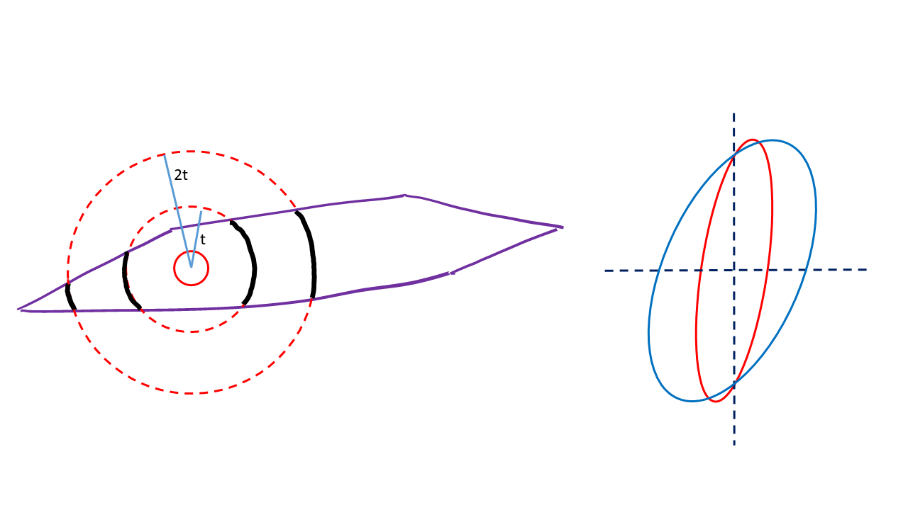
Figure 3.1: (a) Algorithm $\mathsf{IterativeIsotropization}$ uses balls of doubling radii (b) Algorithm $\mathsf{Isotropize}$ scales up the estimated “small eigenvalue” subspace in each iteration.

First, we show that the $p$-th norm of the covariance matrix $\|A\|_{p}$ remains bounded. Although we only use an eigenvalue threshold of $\lambda=n$ in the algorithm, we will prove a slightly more general statement below, assuming the eigenvalue threshold is $\lambda=n/r^{\alpha}$.

Lemma 3.1.

Let $A_{j}$ be the covariance matrix of $TK$ and $r_{j}$ be the inner radius at the $j$-th iteration of algorithm $\mathsf{Isotropize}$. For $\alpha\in[0,2/(p-1)]$, we have

• the number of iterations is $O(\log n)$.

• $\mathrm{Tr}A_{j}=O(r_{j}^{2}\mathrm{Tr}A_{0})$ for all j.

• $\|A_{j}\|_{p}\leq 24nr_{j}^{(\frac{2+\alpha}{p}-\alpha)}\log n$ for all j.

Proof.

In each iteration, the algorithm increases $r_{j}$ by a factor of $2(1-\frac{1}{\log n})$. Note that the algorithm starts with $r_{0}=\frac{1}{4}$ and ends before $r_{j}\log n\leq\sqrt{n}$. Hence, it takes less than $O(\log n)$ iterations.

To bound $\mathrm{Tr}A_{j}$, we let $P_{j}$ be the projection matrix at $j$-th iteration Then the transformation at $j$-th iteration is $M_{j}=I+P_{j}$. We have

$$A_{j}=M_{j}A_{j-1}M_{j}$$ (3.1)

Since $P_{j}$ is a projection matrix, we have

$$\mathrm{Tr}A_{j} =\mathrm{Tr}\left(A_{j-1}^{\frac{1}{2}}M_{j}^{2}A_{j-1}^{\frac{1}{2}}\right)=\mathrm{Tr}\left(A_{j-1}^{1/2}(I+3P_{j})A_{j-1}^{1/2}\right)\leq 4\mathrm{Tr}A_{j-1}.$$

Hence, $\mathrm{Tr}A_{j}$ increases by a factor of at most $4$. Moreover, since $r_{j}$ increases by a factor of $2(1-\frac{1}{\log n})$ we have that $\frac{\mathrm{Tr}A_{j}}{r_{j}^{2}}$ increases by a factor of $(1-\frac{1}{\log n})^{-2}$ per iteration. Since there are $O(\log n)$ iterations, it increases by at most $O(1)$ in total. Hence, we have $\mathrm{Tr}A_{j}=O(r_{j}^{2}\mathrm{Tr}A_{0})=O(r_{j}^{2}n)$ for all $j$.

To bound $\|A_{j}\|_{p}$, we note that initially $\|A_{0}\|_{p}\leq\mathrm{Tr}A_{0}\leq 4n$. By (3.1), we have

$$\|A_{j}\|_{p} =\|M_{j}A_{j-1}M_{j}\|_{p}$$

$$=\|A_{j-1}^{1/2}M_{j}^{2}A_{j-1}^{1/2}\|_{p}$$

$$=\|A_{j-1}^{1/2}(I+3P_{j})A_{j-1}^{1/2}\|_{p}.$$

Hence, we have

$$\|A_{j}\|_{p}\leq\|A_{j-1}\|_{p}+3\|A_{j-1}^{1/2}P_{j}A_{j-1}^{1/2}\|_{p}.$$

Let $\lambda\stackrel{{\scriptstyle\mathrm{{\scriptscriptstyle def}}}}{{=}}\frac{n}{r_{j}^{\alpha}}$. Since $P_{j}$ is the projection of the eigenspace of $\widehat{A}$ with eigenvalues less than $\lambda$, we have that

$$P_{j}\preceq 2\lambda(\widehat{A}+\lambda\cdot I)^{-1}.$$

(To see this, we note that both the sides have the same eigenspace and hence it follows from $1_{x\leq\lambda}\leq\frac{2\lambda}{x+\lambda}$.) By Lemma A.2 with $\epsilon=\frac{1}{2}$, we have that $\frac{1}{2}A_{j}-O(\frac{\log^{3}n\cdot\mathrm{Tr}A_{j}}{k})\cdot I\preceq\widehat{A}.$ Using $\mathrm{Tr}A_{j}=O(r_{j}^{2}n)$ and $k=\Omega(r_{j}^{2+\alpha}\log^{3}n)$ samples, we have

$$A_{j-1}\preceq 2\widehat{A}+\frac{n}{r_{j}^{\alpha}}\cdot I\preceq 2\widehat{A}+\lambda\cdot I.$$

Hence, we have $P_{j}\preceq 4\lambda(A_{j-1}+\lambda\cdot I)^{-1}$ and

$$\|A_{j}\|_{p}\leq\|A_{j-1}\|_{p}+12\lambda\|A_{j-1}^{1/2}(A_{j-1}+\lambda\cdot I)^{-1}A_{j-1}^{1/2}\|_{p}.$$

Let $\lambda_{i}$ be the eigenvalues of $A_{j-1}$. Then,

$$\|A_{j-1}^{1/2}(A_{j-1}+\lambda\cdot I)^{-1}A_{j-1}^{1/2}\|_{p}^{p}=\sum_{i=1}^{n}\left(\frac{\lambda_{i}}{\lambda_{i}+\lambda}\right)^{p}\leq\frac{1}{\lambda^{p}}\sum_{\lambda_{i}\leq\lambda}\lambda_{i}^{p}+\sum_{\lambda_{i}\geq\lambda}1.$$

The first term $\sum_{\lambda_{i}\leq\lambda}\lambda_{i}^{p}$ is maximized when the small eigenvalues are exactly $\lambda_{i}=\lambda$. In this case, there are

$$\frac{\mathrm{Tr}A_{j-1}}{\lambda}\leq\frac{O(r_{j-1}^{2}n)}{\lambda}$$

small eigenvalues, i.e., of value at most $\lambda$. Hence, we have

$$\frac{1}{\lambda^{p}}\sum_{\lambda_{i}\leq\lambda}\lambda_{i}^{p}\leq\frac{O(r_{j-1}^{2}n)}{\lambda}.$$

For the second term,

$$\sum_{\lambda_{i}\geq\lambda}1\leq\frac{\mathrm{Tr}A_{j-1}}{\lambda}\leq\frac{O(r_{j-1}^{2}n)}{\lambda}.$$

Hence, $\|A_{j}\|_{p}$ is increased by

$$O(\lambda)\cdot\left(\frac{r_{j-1}^{2}n}{\lambda}\right)^{1/p}=O\left(\frac{n}{r_{j}^{\alpha}}\right)\cdot\left(r_{j-1}^{2}r_{j}^{\alpha}\right)^{1/p}\leq O\left(nr^{\frac{2+\alpha}{p}-\alpha}\right).$$

Since there are $O(\log n)$ iterations, $\|A_{j}\|_{p}$ is at most $O(nr^{(\frac{2+\alpha}{p}-\alpha)}\log n)$. ∎

Next, we show that the inner radius increases by almost a factor of $2$ every iteration, again for a general choice of eigenvalue threshold $\lambda=n/r^{\alpha}.$

Lemma 3.2.

Algorithm $\mathsf{Isotropize}$ maintains the invariant $\{\|x\|_{2}\leq r\}\subseteq TK$.

Proof.

First, we describe the idea of the proof. When the algorithm modifies the covariance matrix $A$, it estimates the subspace of directions with variance less than $n/r^{\alpha}$ and doubles them. Lemma A.2 shows that

$$\widehat{A}=(1\pm\frac{1}{2})A\pm\frac{n}{2r^{\alpha}}\cdot I.$$

This means, roughly speaking, that any direction that was not doubled satisfies

$$\lambda_{i}\geq\sigma^{2}=\frac{n}{2r^{\alpha}}.$$

So the current body contains an ellipsoid whose axis lengths along the non-doubled directions (call this subspace $V$) are at least $\sigma$ and at least $r$ in all directions (the body contains a ball of radius $r$). Now the body is stretched by a factor of $\sqrt{2}$ in the subspace $V^{\perp}$. We will argue that the resulting body contains a ball of radius nearly $2r$. To see this, we argue that any point in a ball of this radius is in the convex hull of the ball of radius $\sigma$ in the subspace $V$ and a ball of radius $\sqrt{2}r$ in the subspace $V^{\perp}.$

Now we proceed to the formal proof by induction. Initially, we have $\{\|x\|_{2}\leq r\}\subset TK$ by the assumption on $K$. It suffices to show this is maintained after each iteration. Let $T$ be the old transformation and $T^{\prime}$ be the new transformation during one iteration. Let $r$ be the old radius during that iteration. By the invariant, we know that $\{\|x\|_{2}\leq r\}\subset TK$ and hence

$$\{\|M^{-1}x\|_{2}\leq r\}\subset T^{\prime}K$$

with $M=I+P_{\widehat{A}}$ (this only scales up the body by a factor of $2$ in some directions). Let $A$ be the covariance matrix of $TK$. Then $(I+P_{\widehat{A}})A(I+P_{\widehat{A}})$ is the covariance matrix of $T^{\prime}K$. Our goal is to show that $T^{\prime}K$ contains a ball of radius $2(1-\frac{1}{\log n})r$. From above, we have

$$\{x^{\top}A^{-1}x\leq 1\}\subset\{x^{\top}((I+P_{\widehat{A}})A(I+P_{\widehat{A}}))^{-1}x\leq 1\}\subset T^{\prime}K.$$

Hence, we know that $\text{Conv}(\Omega_{1}\cup\Omega_{2})\subset T^{\prime}K$ where

$$\Omega_{1}=\{x^{\top}(\frac{1}{r^{2}}I-\frac{3}{4r^{2}}P_{\widehat{A}})x\leq 1\}\mbox{ and }\Omega_{2}=\{x^{\top}A^{-1}x\leq 1\}.$$

where for $\Omega_{1}$ we used that $(I+P)^{-2}=I-\frac{3}{4}P$ for any projection matrix $P$.

To prove that $T^{\prime}K$ contains a larger ball, we take $x$ and write it as a convex combination of $x_{1}$ and $x_{2}$ where $x_{1}\in\Omega_{1}$ and $x_{2}\in\Omega_{2}$. To do this, we define $P_{A}$ be the projection to the subspace spans by eigenvectors of $A$ with eigenvalues at most $\lambda/2^{8}\log^{2}n$ with

$$\lambda\stackrel{{\scriptstyle\mathrm{{\scriptscriptstyle def}}}}{{=}}\frac{n}{r^{\alpha}}.$$

For any $x$ with $\|x\|_{2}\leq 2(1-\frac{1}{\log n})r$, we will show that $x\in\text{Conv}(\Omega_{1}\cup\Omega_{2})$. To do this, we let $t\stackrel{{\scriptstyle\mathrm{{\scriptscriptstyle def}}}}{{=}}\frac{\|P_{A}x\|_{2}^{2}}{\|x\|_{2}^{2}}$ and write $x$ as the convex combination,

$$x=t\left(\frac{1}{t}P_{A}x\right)+(1-t)\left(\frac{1}{1-t}(I-P_{A})x\right).$$ (3.2)

For the second term in (3.2), we have

$$\left(\frac{1}{1-t}(I-P_{A})x\right)^{\top}A^{-1}\left(\frac{1}{1-t}(I-P_{A})x\right)\leq\frac{\|(I-P_{A})x\|_{2}^{2}}{(1-t)^{2}\lambda/(2^{8}\log^{2}n)}=\frac{2^{8}\|x\|_{2}^{2}\log^{2}n}{\lambda}.$$

Since $\|x\|_{2}^{2}\leq 4r^{2}$ and $\lambda=\frac{n}{r^{\alpha}}$, we have

$$\frac{2^{8}\|x\|_{2}^{2}\log^{2}n}{\lambda}\leq\frac{2^{10}r^{2}\log^{2}n}{\frac{n}{r^{\alpha}}}=\frac{2^{10}r^{2+\alpha}\log^{2}n}{n}\leq 1$$

where the last inequality follows the assumption in the algorithm that $\alpha=0$. Hence,

$$\frac{1}{1-t}(I-P_{A})x\in\Omega_{2}.$$ (3.3)

For the first term in (3.2), we note that for any $\beta>0$, we have

$$P_{\widehat{A}}\succeq\beta\lambda(\beta\lambda\cdot I+\widehat{A})^{-1}-\frac{\beta}{1+\beta}I.$$ (3.4)

(To see this, we note that both sides have the same eigenspace and hence it follows from $1_{x\leq\lambda}\geq\frac{\beta\lambda}{x+\beta\lambda}-\frac{\beta}{1+\beta}$.)

By Lemma A.2 with $\epsilon=1$, we have

$$\widehat{A}\preceq 2A+O\left(\frac{\log^{3}n\cdot\mathrm{Tr}A}{k}\right)\cdot I.$$

Using $\mathrm{Tr}A=O(r^{2}n)$ (Lemma 3.1) and $k=\Omega(r^{2+\alpha}\log^{5}n)$ (the algorithm description), we have

$$\widehat{A}\preceq 2A+\frac{n}{2^{7}r^{\alpha}\log^{2}n}\cdot I\preceq 2A+\frac{\lambda}{2^{7}\log^{2}n}\cdot I.$$

Putting this into (3.4), we have

$$P_{\widehat{A}}\succeq\beta\lambda(\beta\lambda\cdot I+\frac{\lambda}{2^{7}\log^{2}n}+2A)^{-1}-\frac{\beta}{1+\beta}I.$$

On the range of $P_{A}$, we have $A\preceq\frac{\lambda}{2^{8}\log^{2}n}\cdot I$ and hence

$$(P_{A}x)^{\top}P_{\widehat{A}}(P_{A}x)\geq\left(\frac{\beta\lambda}{\beta\lambda+\frac{\lambda}{2^{6}\log^{2}n}}-\frac{\beta}{1+\beta}\right)\|P_{A}x\|_{2}^{2}.$$

Using this, we have

$$f(x) \stackrel{{\scriptstyle\mathrm{{\scriptscriptstyle def}}}}{{=}}\frac{1}{t^{2}r^{2}}(P_{A}x)^{\top}(I-\frac{3}{4}P_{\widehat{A}})(P_{A}x)$$

$$\leq\left(1-\frac{3}{4}\frac{\beta\lambda}{\beta\lambda+\frac{\lambda}{2^{6}\log^{2}n}}+\frac{3}{4}\frac{\beta}{1+\beta}\right)\frac{\|x\|_{2}^{2}}{r^{2}}$$

$$\leq\left(1-\frac{3}{4}\frac{\beta}{\beta+\frac{1}{64\log^{2}n}}+\beta\right)\cdot 4\left(1-\frac{1}{\log n}\right)^{2}$$

where we used $\|x\|_{2}\leq 2(1-\frac{1}{\log n})r$ at the end. Putting $\beta=\frac{1}{8\log n}$, we have

$$f(x) \leq\left(1-\frac{3}{4}\cdot\frac{8\log n}{8\log n+1}+\frac{3}{4}\cdot\frac{1}{1+8\log n}\right)\cdot 4\left(1-\frac{1}{\log n}\right)$$

$$=\left(\frac{7+8\log n}{8\log n+1}\right)\cdot\left(1-\frac{1}{\log n}\right)$$

$$\leq\left(1+\frac{1}{\log n}\right)\cdot\left(1-\frac{1}{\log n}\right)$$

$$\leq 1.$$

Hence from the definition of $\Omega_{1}$, we get

$$\frac{1}{t}P_{A}x\in\Omega_{1}.$$ (3.5)

Combining (3.5) and (3.3), we have

$$x\in\text{Conv}(\Omega_{1}\cup\Omega_{2})\subset T^{\prime}K.$$

Therefore $T^{\prime}K$ contains a ball of radius $2(1-\frac{1}{\log n})r$. This completes the induction. ∎

With the bound on the inner radius and the $p$-norm of the covariance matrix, we can apply Theorem 2.7 and Lemma 2.8 to bound the mixing time and the complexity of the algorithm $\mathsf{Isotropize}$.

Theorem 3.3.

The algorithm $\mathsf{Isotropize}$ applied to a well-rounded input convex body $K$ satisfying $B(0,1)\subseteq K$ with $\mathbb{E}_{K}\left\|x\right\|^{2}=O(n)$, with high probability, finds a transformation $T$ using $\widetilde{O}(n^{3}\psi^{2})$ oracle calls, s.t. $TK$ is $2$-isotropic.

Proof.

Theorem 2.9 shows that it takes $\widetilde{O}(n^{3})$ to get the first sample from a well-rounded body with Gaussian Cooling. (Note that a uniform point from $K_{t}$ would be a very bad warm start for $K_{2t}$.) This gives a warm start for all subsequent steps.

Let $A_{j}$ be the covariance matrix in the $j$-th iteration of the algorithm. By Lemma 3.1 with $\alpha=0$, we have that

$$\left\|A_{j}\right\|_{p}\leq O(nr^{2/p}\log n).$$

In the $j$-th iteration, the algorithm samples $k=c\cdot r_{j}^{2}\log^{5}n$ points. To bound the sampling cost, first note that for distribution $q$ with KLS constant $\psi_{q}$, the complexity per sample is $\widetilde{O}(n^{2}\psi_{q}^{2}/r_{j}^{2})$ since by Lemma 3.2, the algorithm maintains a ball of radius $r_{j}$ inside the body. Suppose that the KLS constant for isotropic distributions is $\psi$. We choose $p$ so that $\psi^{2}=O(n^{1/p})$. By Lemma 2.8 with $\beta=1/2p$, this implies that the KLS constant even for non-isotropic distributions with covariance $A$ satisfies $\psi_{q}^{2}=O(\left\|A\right\|_{p}\log n)$. Lemma 2.7 shows that the total complexity of the $j$-th iteration is at most

$$c\cdot r_{j}^{2}\cdot\widetilde{O}\left(\frac{n^{2}\cdot\left\|A_{j}\right\|_{p}}{r_{j}^{2}}\right)\leq\widetilde{O}\left(n^{3}r_{j}^{2/p}\right)=\widetilde{O}\left(n^{3+\frac{1}{p}}\right).$$

since we stop with $r^{2}=O(n)$. By the definition of $p$, the complexity is $\widetilde{O}(n^{3}\psi^{2})$. For the cost of computing covariance matrix and the mean, Lemma 2.5 shows that WHP $O(n)$ samples suffice for a constant factor estimate of the covariance. The total cost is

$$n\cdot\widetilde{O}(n^{2}\cdot\left\|A\right\|_{p}r^{-2})=r^{2}\cdot\widetilde{O}(n^{2}\cdot\left\|A\right\|_{p}r^{-2})=\widetilde{O}\left(n^{3+\frac{1}{p}}\right)$$

where we used that $n=\widetilde{O}(r^{2})$ at the end of the algorithm. ∎

3.2 Outer loop: the general case

For the general case, we first show that the next body is well-rounded after each iteration and hence satisfies the condition of the algorithm $\mathsf{Isotropize}$. The proof is an adaptation of a proof from [26, Lemma 5.4].

Lemma 3.4.

Suppose that for a convex body $K$, the set $K\cap B(0,t)$ is $2$-isotropic. Then $K\cap B(0,2t)$ is well-rounded.

Proof.

Let $K_{t}=K\cap B(0,t)$ and $K_{2t}=K\cap B(0,2t)$. Since $K_{t}$ is $2$-isotropic, $K_{t}$ has mean $0$ with $I\preceq\mathbb{E}_{x\in K_{t}}xx^{\top}\preceq 2I$. Hence, $K_{t}$ contains the unit ball of radius $1$. Let $t_{\text{small}}=2\sqrt{n}$ and $K_{t_{\text{small}}}=K\cap B(0,t_{\text{small}})$. If $2t\leq 3t_{\text{small}}$ then clearly $\mathbb{E}_{K_{2t}}\left\|x\right\|^{2}\leq(6\sqrt{n})^{2}=36n$ and we are done. Otherwise, $t>3t_{\text{small}}/2$. Let $\lambda$ be such that

$$t=\lambda t_{\text{small}}+(1-\lambda)2t.$$

Note that $\lambda=\frac{2t-t}{2t-t_{\text{small}}}\leq\frac{t}{4t/3}=\frac{3}{4}.$ By the Brunn-Minkowski inequality, we have

$$\mathrm{vol}(K_{t})^{1/n}\geq\lambda\mathrm{vol}(K_{t_{\text{small}}})^{1/n}+(1-\lambda)\mathrm{vol}(K_{2t})^{1/n}.$$ (3.6)

Next, by the choice of $t_{\text{small}}$, since $K_{t}$ is $2$-isotropic, using Paouris’ inequality (Lemma 2.4), we have

$$\mathrm{vol}(K_{t})\leq\mathrm{vol}(K_{t_{\text{small}}})(1+\exp(-c\sqrt{n}))$$

for some constant $c$. Using this with (3.6), we have

$$\mathrm{vol}(K_{2t}) \leq\left(\frac{\mathrm{vol}(K_{t})^{1/n}-\lambda\mathrm{vol}(K_{t_{\text{small}}})^{1/n}}{1-\lambda}\right)^{n}$$

$$\leq\mathrm{vol}(K_{t_{\text{small}}})\left(\frac{(1+\exp(-c\sqrt{n}))^{1/n}-\lambda}{1-\lambda}\right)^{n}$$

$$\leq\mathrm{vol}(K_{t_{\text{small}}})\left(1+\frac{8}{n}\exp(-c\sqrt{n})\right)^{n}$$

$$\leq\mathrm{vol}(K_{t_{\text{small}}})\left(1+16\exp(-c\sqrt{n})\right).$$

Thus, the fraction of the volume of $K_{2t}$ that lies outside a ball of radius $t_{\text{small}}$ is exponentially small. Moreover, since $K_{t}$ is 2-isotropic, all of $K_{t}$ lies in a ball of radius $2n$ and $0\in K_{t}$. Moreover, $0\in K_{2t}$ and since $K_{2t}=K\cap B(0,2t)\subseteq 2(K\cap B(0,t))=2K_{t}$, we have that $K_{2t}$ lies in a ball of radius $4n$.

$$\mathbb{E}_{K_{2t}}\left\|x\right\|^{2}\leq t_{\text{small}}^{2}+(4n)^{2}\cdot 16\exp(-c\sqrt{n})=5n.$$

∎

Now we are ready to prove the main theorem about rounding.

Proof of Theorem 1.5..

The initial body $K_{r}$ is a ball, and at the end of the first iteration, the body is $2$-isotropic. Let $K_{t}$ be the convex body in some iteration. Assume that $K_{t}$ is $2$-isotropic. By Lemma 3.4, $K_{2t}$ is well-rounded. Since $(K_{t}-x)$ contains a unit ball, so does $(K_{2t}-x)$. Then by Theorem 3.3 the inner loop to make $K_{2t}$ near-isotropic takes $\tilde{O}(n^{3}\psi^{2})$ oracle queries. Since the number of iterations of the outer loop is only $\log(R/r)$, the theorem follows. ∎

4 Polytope Volume

In this section, we consider the special case of convex polytopes. We assume that a polytope $P=\left\{x:Ax\leq b\right\}$ is given explicitly by $A\in R^{m\times n},b\in R^{m}$. A naive implementation of the our general membership oracle algorithm would take $O(mn)$ arithmetic operations per oracle call, leading to a time bound of $\widetilde{O}(mn^{4+o(1)})$, where the first term is the time complexity from the oracle queries and the second term is from the additional arithmetic operations per oracle query. This is now the number of arithmetic operations. This already improves the current best time complexity for polytopes using earlier volume algorithms and an amortization trick introduced in [27]. Here we give two significantly faster implementations. The first algorithm is based on a very simple application of fast matrix multiplication. Since fast matrix multiplication is practical only for very high dimension, we also give a different implementation extending the ideas of [27].

4.1 An efficient implementation using Fast Matrix Multiplication

We can replace every ball walk sampling step with the following algorithm.

Algorithm 3 Polytope Ball Walk

1:procedure $\mathsf{PolytopeBallWalk}$($A\in\mathbb{R}^{m\times n},b\in\mathbb{R}^{m},x_{0}\in\mathbb{R}^{n},\delta>0,k\in\mathbb{N}$)

2:     Assumption: $Ax_{0}\leq b$.

3:     Sample points $z_{1},\dots,z_{k}$ from $B_{n}(0,\delta)$.

4:     $Z\leftarrow\begin{pmatrix}z_{1}&z_{2}&\cdots&z_{k}\end{pmatrix},Y\leftarrow AZ$.

5:     $x\leftarrow x_{0},y\leftarrow Ax_{0}$.

6:     for $i\leftarrow 1:k$ do

7:         if $y+Y_{i}\leq b$. then

8:              $x\leftarrow x+z_{i},y\leftarrow y+Y_{i}$.

9:         end if

10:     end for

11:     Return ($x$).

12:end procedure

Next, we show that this algorithm will improve the running time of the ball walk.

Lemma 4.1.

Given a polytope $\{x\in\mathbb{R}^{n}:Ax\leq b\}$ where $A\in\mathbb{R}^{m\times n}$, $k$ steps of the ball walk in the polytope can be implemented in time $O(C(m,n,k))$ where $C(m,n,k)$ denotes the minimum number of arithmetic operations needed to multiply an $m\times n$ matrix by an $n\times k$ matrix.

Proof.

We can see that Algorithm 3 does the same computations as the ball walk algorithm with step size $\delta$ and run for $k$ steps. The only difference is that we generate the random vectors from $B(0,\delta)$ first and do a preprocessing step to avoid multiplying $Az_{i}$ at each step. So the resulting point will be the same as the ball walk algorithm and we reduce the running time of each step.

Let $Z,Y,x,y$ be the same as in Algorithm 3. Generating $k$ random vectors will cost $O(nk)$. For each step, we compute $y+Y_{i}$ in $O(m)$ time and $x+z_{i}$ in $O(n)$ time. So the total time taken is

$$O(nk)+C(m,n,k)+O((m+n)k)=O(C(m,n,k)).$$

∎

We will apply this speedup to the polytope volume computation. From Theorem 3.3, in the $j$-th iteration of Isotropiztion, we run ball walk for $k=\widetilde{O}(n^{3})$ steps with the same transformation matrix $T$, and hence we can use the above algorithm to improve running time.

For getting the first sample, we use the Gaussian Cooling algorithm which in turn runs ball walk in phases with different ball radii and target distributions. However, the total number of ball walk steps in the Gaussian Cooling algorithm for a well-rounded body is $\tilde{O}(n^{3})$ and we also know the maximum number of steps needed for each phase. Therefore, we can construct the matrix $Z$ in Algorithm 3 with $k=\tilde{O}(n^{3})$. The following lemma gives the current best matrix bounds from [31], [17], and [16]. For $k>0$, define the exponent of the rectangular matrix multiplication as follows:

$$\omega(1,1,k)=\inf\{\tau\in\mathbb{R}\mid C(n,n,\lfloor n^{k}\rfloor)=O(n^{\tau})\}.$$

Fact 4.2 ([31],[17],[16]).

$\omega(1,1,3)=4.199712$.

To prove the first part of Theorem 1.7, use Algorithm 3. For $1/p=o(1)$, the total time is $\widetilde{O}(mn^{\omega(1,1,3)-1+o(1)})=\widetilde{O}(mn^{3.199712+o(1)})$.

4.2 Implementation with an amortized Ball Walk

We can also speed up the algorithm by using an implementation of the ball walk for polytopes introduced by [27]. For a body in near-isotropic position, it requires only an expected $O(m)$ operations per step from a warm start.

The main idea of the algorithm is when moving from a point $x\in K$ to $y$, instead of checking the distance between the point $y$ and every constraint $\left(a_{j},b_{j}\right)$ of the polytope at every step, we check the distance from a constraint at only a fraction of the steps. Firstly, with high probability, the step size along any constraint direction $a_{j}$ is bounded by $O^{*}(\frac{\delta}{\sqrt{n}})=O^{*}(\frac{1}{n})$. This can be used to determine which constraint to check at the current step by maintaining a probabilistic lower bound on $h_{j}(x)=b_{j}-a_{j}^{\top}x$, the distance between the current point and the $j$-th constraint. Then, a constraint is checked at the current step only if the corresponding lower bound is $O(\frac{1}{n})$. The last ingredient of their analysis is an anti-concentration bound which states that the probability of the distance between a uniform point from an isotropic convex body and a hyperplane being less than $\epsilon$ is $O(\epsilon)$. This ensures that we need to check only $O(m/n)$ constraints in expectation at every step for an isotropic polytope.

However, in our algorithm, the intermediate polytopes are not near-isotropic but well-rounded. The aforementioned probability is inversely proportional to the standard deviation of the body in that direction, which can be as small as $\frac{r}{n}$. We extend the anti-concentration bound to convex polytopes containing a ball of radius $r$, i.e., the probability that a uniform point from such a polytope is at a distance less than $\epsilon$ from any hyperplane is $O(\frac{n\epsilon}{r})$ which ensures that we need to check only $O\left(\frac{m}{r}\right)$ constraints in expectation at every step of this modified ball walk. Since the number of points sampled in the $j$-th iteration of Isotropize is $\tilde{O}(r^{2})$, this still gives runtime savings because we sample fewer points for smaller values of $r$ and save asymptotically.

Algorithm 4 Amortized Ball Walk for Polytopes[27]

1:procedure $\mathsf{ModifiedBallWalk}$($A\in\mathbb{R}^{m\times n},b\in\mathbb{R}^{m},x_{0}\in\mathbb{R}^{n},\rho>0,\delta>0,N\in\mathbb{N}$)

2:     Assumption: $Ax_{0}\leq b$ and $\left\|x\right\|_{2}<\rho$.

3:     $d_{j}=b_{j}-a_{j}^{\top}x_{0}$ for $j\in[m]$.

4:     Sort $d_{j}$’s in ascending order in an array $H$.

5:     for $i\leftarrow 0:N$ do

6:         $y_{i+1}\sim B(x_{i},\delta)$.

7:         if $\left\|y_{i+1}\right\|_{2}>\rho$ then

8:              $x_{i+1}=x_{i}$

9:         end if

10:         Let $j^{*}$ be the largest $j$ such that $d_{j^{*}}\leq\alpha\cdot\frac{\delta}{\sqrt{n}}\cdot i$ $\triangleright$ $\alpha=4\log\left(\frac{2mN}{\epsilon}\right)$

11:         for $k=1\to j^{*}$ do

12:              $d_{k}=b_{k}-a_{k}^{\top}y_{i+1}$.

13:              if $d_{k}<0$ then

14:                  $x_{i+1}=x_{i}$.

15:              end if

16:              Insert $d_{k}+\alpha\cdot\frac{\delta}{\sqrt{n}}\cdot i$ in $H$ in sorted order.

17:         end for

18:         $x_{i+1}=y_{i+1}$.

19:     end for

20:     Return $x_{N}$.

21:end procedure

Before proving the anti-concentration lemma, we need a result relating the radius of a ball inside a convex body $K$ and the minimum eigenvalue of the covariance matrix of $K$.

Lemma 4.3.

For a convex body $K\subseteq\mathbb{R}^{n}$ containing a ball of radius $r$, the minimum eigenvalue of its covariance matrix is at least $\frac{r^{2}}{(n+1)^{2}}$.

Proof.

Let $\Sigma=\mathbb{E}_{K}[(x-\mu)(x-\mu)^{\top}]$ and $\sigma$ be the minimum eigenvalue of $\Sigma$ and $y$ be the corresponding eigenvector with unit $\ell_{2}$-norm. Then,

$$\sigma =\min_{z\neq 0,\|z\|_{2}=1}z^{\top}\Sigma z$$

$$=\min_{z\neq 0,\|z\|_{2}=1}z^{\top}\mathbb{E}_{K}[(x-\mu)(x-\mu)^{\top}]z$$

$$=\min_{z\neq 0,\|z\|_{2}=1}\mathbb{E}_{K}[(z^{\top}(x-\mu))^{2}]$$

$$=\mathbb{E}_{K}[(y^{\top}(x-\mu))^{2}].$$

WLOG, let $\mu=0$ and let $v$ be the point in $K$ which maximizes $|y^{\top}v|$. Since $K$ contains a ball of radius $r$, $|y^{\top}v|\geq r$. Let $\partial B$ denote the $(n-1)$-dimensional sphere. For any $u\in\partial B$, let $\phi(u)$ denote the largest real number $t$ such that $v+tu\in K$. Then we have,

$$\mathrm{vol}(K)=\int_{\partial B}\int_{0}^{\phi(u)}t^{n-1}dtdu=\frac{1}{n}\int_{\partial B}\phi(u)^{n}du$$

and

$$\sigma =\frac{1}{\mathrm{vol}(K)}\int_{K}(y^{T}x)^{2}dx$$

$$=\frac{1}{\mathrm{vol}(K)}\int_{\partial B}\int_{0}^{\phi(u)}t^{n-1}(y^{T}(v+tu))^{2}dtdu$$

$$=\frac{1}{\mathrm{vol}(K)}\int_{\partial B}\left(\frac{\phi(u)^{n}}{n}(y^{T}v)^{2}+2\frac{\phi(u)^{n+1}}{n+1}(y^{T}v)(y^{T}u)+\frac{\phi(u)^{n+2}}{n+2}(y^{T}u)^{2}\right)du$$

$$=\frac{1}{\mathrm{vol}(K)}\int_{\partial B}\frac{\phi(u)^{n}}{n(n+1)^{2}}(y^{T}v)^{2}+\frac{\phi(u)^{n}}{n}\left(\sqrt{\frac{n}{n+2}}\phi(u)y^{T}u+\frac{\sqrt{n(n+2}}{n+1}y^{T}v\right)^{2}du$$

$$\geq\frac{1}{\mathrm{vol}(K)}\int_{\partial B}\frac{\phi(u)^{n}}{n(n+1)^{2}}(y^{T}v)^{2}du$$

$$\sigma \geq\frac{1}{(n+1)^{2}}(y^{T}v)^{2}\geq\frac{r^{2}}{\left(n+1\right)^{2}}.$$

∎

Lemma 4.4 (Anti-concentration).

For a convex body $K\subseteq\mathbb{R}^{n}$ with uniform distribution $\pi_{K}$ and covariance matrix $\Sigma\succeq\sigma^{2}I$, let $X\sim\pi_{K}$ be a random point distributed uniformly on $K$. Then for any hyperplane $H\subseteq\mathbb{R}^{n}$, we have

$$\Pr\left[\mathrm{dist}(X,H)\leq\epsilon\right]\leq\frac{2\epsilon}{\sigma}\quad\forall\epsilon>0.$$

Proof.

Let $H=\left\{x\in\mathbb{R}^{n}:ax=b\right\}$ with $a\in\mathbb{R}^{1\times n},\left\|a\right\|_{2}=1$ and $b\in\mathbb{R}$. For $X\sim\pi_{K}$, let the distribution of $aX$ be denoted by $\pi_{K}^{a}$. Then $\pi_{K}^{a}$ is logconcave with variance $a\Sigma a^{\top}=\sigma_{1}^{2}\geq\sigma^{2}$. Let $\hat{\pi}_{K}^{a}$ denote the distribution of $\frac{1}{\sigma_{1}}aX$. Then $\hat{\pi}_{K}^{a}$ is isotropic and logconcave. If $x^{*}$ is the maximizer of $\hat{\pi}_{K}^{a}$, then

$$\hat{\pi}_{K}^{a}(x^{*})\leq 1.$$

For any $\epsilon>0$,

$$\Pr\left[|aX-b|\leq\epsilon\right] =\Pr\left[\frac{|aX-b|}{\sigma_{1}}\leq\frac{\epsilon}{\sigma_{1}}\right]$$

$$=\int_{\frac{b-\epsilon}{\sigma_{1}}}^{\frac{b+\epsilon}{\sigma_{1}}}\hat{\pi}_{K}^{a}(x)dx\leq\int_{\frac{b-\epsilon}{\sigma_{1}}}^{\frac{b+\epsilon}{\sigma_{1}}}\hat{\pi}_{K}^{a}(x^{*})dx$$

$$\leq\int_{\frac{b-\epsilon}{\sigma_{1}}}^{\frac{b+\epsilon}{\sigma_{1}}}dx=\frac{2\epsilon}{\sigma_{1}}\leq\frac{2\epsilon}{\sigma}.$$

∎

Lemma 4.5 (Frequency of constraint checking).

For a polytope $K$ with covariance matrix $\Sigma\geq\sigma^{2}I$ and Ball Walk with step size $\delta$ and tolerance parameter $\alpha$, suppose that the initial point $X_{0}$ is $\beta$-warm with respect to the uniform distribution for some $\beta>0$. Let $N_{j}$ be the number of steps (excluding the first step) of the modified Ball Walk Markov chain at which the algorithm checks inequality $(A_{j},b_{j})$ and let $N$ be the number of Markov chain steps. Let $F_{j}:=\frac{N_{j}}{N}$. Then,

$$\mathbb{E}[F_{j}]=16\frac{\alpha\beta\delta}{\sqrt{n}\sigma}(1+2\log(n))+\frac{\beta\epsilon}{N}.$$

This lemma follows directly from Lemma 4.5 in [27] using the anti-concentration bound from Lemma 4.4.

Lemma 4.6.

The algorithm $\mathsf{Isotropize}$ applied to a well-rounded convex polytope $K$ containing $B(0,1)$, with high probability, finds a transformation $T$, s.t. $TK$ is $2$-isotropic using $\tilde{O}(n^{3}\psi^{2})$ oracle calls and $\tilde{O}(mn^{4})$ arithmetic operations.

Proof.

It takes $\tilde{O}(n^{3})$ steps of the Gaussian Cooling algorithm to get the first sample from a well-rounded body where every step can be implemented in $O(mn)$ arithmetic operations. Let $A_{j}$ and $r_{j}$ be the covariance matrix and the inner radius at the $j$-th iteration of the algorithm respectively. From Theorem 3.3, the number of oracle calls in the $j$-th iteration of the algorithm is $\tilde{O}(n^{3}r_{j}^{\frac{2}{p}})$. So, the total complexity of $j$-th iteration is at most

$$\tilde{O}(n^{3}r_{j}^{\frac{2}{p}})\cdot\tilde{O}(mnr_{j}^{-1})\leq\tilde{O}(mn^{4}r^{\frac{2}{p}-1}).$$

Since we stop before $2^{10}r^{2}\log n=n$, the total complexity of the algorithm is

$$\tilde{O}\left(mn^{4}+mn^{3+\frac{1}{p}}\right),$$

which is $\tilde{O}(mn^{4})$. ∎

Given a convex polytope $K$, we can use Algorithm 4 to make it near-isotropic and then use the Gaussian Cooling algorithm [6] to compute its volume. The second part of Theorem 1.7 (without fast matrix multiplication) follows.

Appendix A Empirical Covariance Matrix with Sublinear Sample Complexity

To bound the error of the empirical covariance matrix $A$, we use the following matrix Chernoff bound.

Lemma A.1 (Matrix Bernstein [30, Theorem 6.1]).

Consider a finite sequence $\{X_{i}\}$ of independent, random, self-adjoint matrices of dimension $n$. Assume that $\mathbb{E}X_{i}=0$ and $\|X_{i}\|_{\mathrm{op}}\leq R$ almost surely. Then, for all $t\geq 0$, we have

$$\mathbb{P}\left(\|\sum_{i}X_{i}\|_{\mathrm{op}}\geq t\right)\leq 2n\exp\left(\frac{-t^{2}/2}{\sigma^{2}+Rt/3}\right)$$

where $\sigma^{2}\stackrel{{\scriptstyle\mathrm{{\scriptscriptstyle def}}}}{{=}}\|\sum_{i}\mathbb{E}(X_{i}^{2})\|_{\mathrm{op}}.$

Lemma A.2.

Let $p$ be a logconcave density in $\mathbb{R}^{n}$ with covariance $A$. Let $\widehat{A}\leftarrow\frac{1}{k}\sum_{i=1}^{k}(x_{i}-\widehat{x})(x_{i}-\widehat{x})^{\top}$ where $\widehat{x}=\frac{1}{k}\sum_{i=1}^{k}x_{i+k}$ and $x_{i}$ are independent samples from $p$. With probability $1-1/n^{O(1)}$, for any $0\leq\epsilon\leq 1$, we have

$$(1-\epsilon)A-O\left(\frac{\log^{3}n\mathrm{Tr}A}{\epsilon k}\right)\cdot I\preceq\widehat{A}\preceq(1+\epsilon)A+O\left(\frac{\log^{3}n\cdot\mathrm{Tr}A}{\epsilon k}\right)\cdot I.$$

Remark.

By a more careful tail analysis, one can get a bound of $O(\frac{\log n\cdot\mathrm{Tr}A}{\epsilon k})\cdot I$ and we speculate that the tight bound for the additive term might be $O(\frac{\mathrm{Tr}A}{\epsilon k})\cdot I$.

Proof.

Let $\lambda\geq 0$ to some constant to be determined. By shifting the distribution, we can assume $p$ has mean $0$. Let $\widetilde{p}$ be the distribution given by $p$ restricted to the ball

$$\{\|x\|_{(\lambda A+I)^{-1}}\leq 3s\cdot\sqrt{\mathrm{Tr}(\lambda A+I)^{-\frac{1}{2}}A(\lambda A+I)^{-\frac{1}{2}}}\}$$

for some $s=\Theta(\log n)$. Using the fact that $p$ has mean $0$ and the fact that $(\lambda A+I)^{-\frac{1}{2}}A(\lambda A+I)^{-\frac{1}{2}}\preceq A$, Lemma 2.3 shows that

$$\mathbb{P}_{x\sim p}(\|x\|_{(\lambda A+I)^{-1}}\leq 3s\cdot\sqrt{\mathrm{Tr}A})\geq 1-\frac{1}{n^{\Theta(1)}}.$$

Let $A_{i}$ be the random matrices $(x_{i}-\widehat{x})(x_{i}-\widehat{x})^{\top}$ with $x_{i}$ sampled from $p$ and $\widetilde{A}_{i}$ be the random matrices $(\widetilde{x}_{i}-\widehat{x})(\widetilde{x}_{i}-\widehat{x})^{\top}$ with $\widetilde{x}_{i}$ sampled from $\widetilde{p}$. Note that when $k=\Omega(n)$, we have that WHP $\frac{1}{2}A\preceq\widehat{A}\preceq 2A$ 2.5. Hence, we can assume $k=O(n)$. We couple two matrices together such that $\widetilde{A}_{i}=A_{i}$ for $i=1,2,\cdots k$ with probability $1-ke^{-s}=1-\frac{1}{n^{\Theta(1)}}$. Let $X_{i}=\frac{1}{k}(\lambda A+I)^{-\frac{1}{2}}(A_{i}-\mathbb{E}A_{i})(\lambda A+I)^{-\frac{1}{2}}$ and $\widetilde{X}_{i}=\frac{1}{k}(\lambda A+I)^{-\frac{1}{2}}(\widetilde{A}_{i}-\mathbb{E}\widetilde{A}_{i})(\lambda A+I)^{-\frac{1}{2}}$ for some $\lambda$ to be chosen where the expectation $\mathbb{E}$ is conditional on $\hat{x}$. Note that

$$\mathbb{P}(\left\|(\lambda A+I)^{-\frac{1}{2}}(\widehat{A}-\mathbb{E}\widehat{A})(\lambda A+I)^{-\frac{1}{2}}\right\|_{\mathrm{op}}\geq t) =\mathbb{P}(\|\sum_{i}X_{i}\|_{\mathrm{op}}\geq t)$$

$$\leq\mathbb{P}(\|\sum_{i}\widetilde{X}_{i}\|_{\mathrm{op}}\geq t)+\frac{1}{n^{\Theta(1)}}.$$ (A.1)

Hence, it suffices to study $\widetilde{X}_{i}$.

We will apply Lemma A.1. For the sup norm bound, note that

$$\|\widetilde{X}_{i}\|_{\mathrm{op}} \leq\frac{1}{k}\left(\|(\lambda A+I)^{-\frac{1}{2}}\widetilde{A}_{i}(\lambda A+I)^{-\frac{1}{2}}\|_{\mathrm{op}}+\|(\lambda A+I)^{-\frac{1}{2}}\mathbb{E}\widetilde{A}_{i}(\lambda A+I)^{-\frac{1}{2}}\|_{\mathrm{op}}\right)$$

$$\leq\frac{1}{k}\left(\|\widetilde{x}_{i}-\widehat{x}\|_{(\lambda A+I)^{-1}}^{2}+\mathbb{E}\|\widetilde{x}_{i}-\widehat{x}\|_{(\lambda A+I)^{-1}}^{2}\right)$$

$$\leq\frac{1}{k}\left(2\|\widetilde{x}_{i}\|_{(\lambda A+I)^{-1}}^{2}+2\mathbb{E}\|\widetilde{x}_{i}\|_{(\lambda A+I)^{-1}}^{2}+4\|\widehat{x}\|_{(\lambda A+I)^{-1}}^{2}\right)$$

$$\leq\frac{4}{k}\left(9s^{2}\mathrm{Tr}A+\|\widehat{x}\|_{(\lambda A+I)^{-1}}^{2}\right)\leq R$$

where the second inequality follows from the fact that non-zero eigenvalues of $Y^{T}Y$ and $YY^{T}$ are the same for any rectangular matrix $Y$, and

$$R\stackrel{{\scriptstyle\mathrm{{\scriptscriptstyle def}}}}{{=}}\frac{36}{k}\left(s^{2}\mathrm{Tr}A+\|\widehat{x}\|_{(\lambda A+I)^{-1}}^{2}\right)$$ (A.2)

For the variance bound, note that $(\lambda A+I)^{-\frac{1}{2}}\widetilde{A}_{i}(\lambda A+I)^{-\frac{1}{2}}\preceq kR$ and hence (using again that $(a-b)^{2}\leq 2(a^{2}+b^{2}))$,

$$\mathbb{E}\widetilde{X}_{i}^{2} \preceq\mathbb{E}\frac{2}{k^{2}}(((\lambda A+I)^{-\frac{1}{2}}\widetilde{A}_{i}(\lambda A+I)^{-\frac{1}{2}})^{2}+(\mathbb{E}(\lambda A+I)^{-\frac{1}{2}}\widetilde{A}_{i}(\lambda A+I)^{-\frac{1}{2}})^{2})$$

$$\preceq\frac{2kR}{k^{2}}\mathbb{E}((\lambda A+I)^{-\frac{1}{2}}\widetilde{A}_{i}(\lambda A+I)^{-\frac{1}{2}}+\mathbb{E}((\lambda A+I)^{-\frac{1}{2}}\widetilde{A}_{i}(\lambda A+I)^{-\frac{1}{2}})$$

$$=\frac{4R}{k}\mathbb{E}(\lambda A+I)^{-\frac{1}{2}}\widetilde{A}_{i}(\lambda A+I)^{-\frac{1}{2}}$$

$$\preceq\frac{8R}{k}\mathbb{E}(\lambda A+I)^{-\frac{1}{2}}A_{i}(\lambda A+I)^{-\frac{1}{2}}$$

$$=\frac{8R}{k}(\frac{A}{\lambda A+I}+(\lambda A+I)^{-\frac{1}{2}}\widehat{x}\widehat{x}^{\top}(\lambda A+I)^{-\frac{1}{2}})$$

where we used that $\frac{d\widetilde{p}}{dp}\leq 2$ in the last inequality. Hence, we have

$$\sigma^{2}\stackrel{{\scriptstyle\mathrm{{\scriptscriptstyle def}}}}{{=}}\|\sum_{i}\mathbb{E}\widetilde{X}_{i}^{2}\|_{\mathrm{op}}\leq 8R(\|\frac{A}{\lambda A+I}\|_{\mathrm{op}}+\|\widehat{x}\|_{(\lambda A+I)^{-1}}^{2}).$$

Apply Lemma A.1, with probability $1-\frac{1}{n^{\Theta(1)}}$, we have

$$\|\sum_{i}\widetilde{X}_{i}\|_{\mathrm{op}} \lesssim\sigma\sqrt{\log n}+R\log n$$

$$\lesssim\sqrt{(\|\frac{A}{\lambda A+I}\|_{\mathrm{op}}+\|\widehat{x}\|_{(\lambda A+I)^{-1}}^{2})}\sqrt{R\log n}+R\log n$$

Using the value of $R$ from equation A.2, for any $c\geq 1$, we get

$$\|\sum_{i}\widetilde{X}_{i}\|_{\mathrm{op}} \lesssim\frac{1}{c}\|\frac{A}{\lambda A+I}\|_{\mathrm{op}}+\frac{1}{c}\|\widehat{x}\|_{(\lambda A+I)^{-1}}^{2}+\frac{c}{k}(\log^{2}n\cdot\mathrm{Tr}A+\|\widehat{x}\|_{(\lambda A+I)^{-1}}^{2})\log n$$

$$\lesssim\frac{1}{c\lambda}+(\frac{1}{c}+\frac{c\log n}{k})\cdot\|\widehat{x}\|_{(\lambda A+I)^{-1}}^{2}+\frac{c\log^{3}n}{k}\cdot\mathrm{Tr}A$$

Using this and equation (A.1) , we have

$$\left\|(\lambda A+I)^{-\frac{1}{2}}(\widehat{A}-\mathbb{E}\widehat{A})(\lambda A+I)^{-\frac{1}{2}}\right\|_{\mathrm{op}}\lesssim\frac{1}{c\lambda}+(\frac{1}{c}+\frac{c\log n}{k})\cdot\|\widehat{x}\|_{(\lambda A+I)^{-1}}^{2}+\frac{c\log^{3}n}{k}\cdot\mathrm{Tr}A.$$

Finally, we note that $\widehat{x}$ follows a logconcave distribution with mean $0$ and covariance matrix $\frac{1}{k}A$. By Lemma 2.3, we have that

$$\|\widehat{x}\|_{(\lambda A+I)^{-1}}\lesssim\log n\sqrt{\frac{1}{k}\mathrm{Tr}A}$$

with probability $1-1/n^{O(1)}$. This gives

$$\left\|(\lambda A+I)^{-\frac{1}{2}}(\widehat{A}-\mathbb{E}\widehat{A})(\lambda A+I)^{-\frac{1}{2}}\right\|_{\mathrm{op}} \lesssim\frac{1}{c\lambda}+(\frac{\log^{2}n}{ck}+\frac{c\log^{3}n}{k})\cdot\mathrm{Tr}A$$

$$\lesssim\frac{1}{c\lambda}+\frac{c\log^{3}n}{k}\cdot\mathrm{Tr}A$$

Hence, we have

$$|\widehat{A}-\mathbb{E}\widehat{A}|\lesssim\frac{1}{c}A+\frac{1}{c\lambda}I+\frac{c\log^{3}n}{k}\cdot\mathrm{Tr}A\cdot(\lambda A+I).$$

Taking $c=\Theta(\epsilon^{-1})$, $\lambda=\frac{k}{c^{2}\log^{3}n\mathrm{Tr}A}$, we have

$$|\widehat{A}-\mathbb{E}\widehat{A}|\preceq\epsilon A+O(\frac{\log^{3}n\mathrm{Tr}A}{\epsilon k})\cdot I.$$

The result follows using $\mathbb{E}\widehat{A}=A$. ∎

Appendix B Proof of the anisotropic KLS bound

Consider the following stochastic localization process.

Definition B.1.

For a logconcave density $p$, we define the following stochastic differential equation:

$$c_{0}=0,\quad dc_{t}=dW_{t}+\mu_{t}dt,$$ (B.1)

where the probability density $p_{t}$, the mean $\mu_{t}$ and the covariance $A_{t}$ are defined by

$$p_{t}(x)=\frac{e^{c_{t}^{\top}x-\frac{t}{2}\left\|x\right\|_{2}^{2}}p(x)}{\int_{\mathbb{R}^{n}}e^{c_{t}^{\top}y-\frac{t}{2}\left\|y\right\|_{2}^{2}}p(y)dy},\quad\mu_{t}=\mathbb{E}_{x\sim p_{t}}x,\quad A_{t}=\mathbb{E}_{x\sim p_{t}}(x-\mu_{t})(x-\mu_{t})^{\top}.$$

The following lemma shows that one can upper bound the expansion $\psi_{p}$ by upper bounding $\|A_{t}\|_{\mathrm{op}}$:

Lemma B.2 ([19, Lemma 31 in ArXiv ver 3]).

Given a logconcave density $p$, let $A_{t}$ be as in Definition B.1 using initial density $p$. Suppose there is a $T>0$ such that

$$\mathbb{P}\left(\int_{0}^{T}\left\|A_{s}\right\|_{\mathrm{op}}ds\leq\frac{1}{64}\right)\geq\frac{3}{4}$$

Then, we have $\psi_{p}=O\left(T^{-1/2}\right).$

To bound $\|A_{t}\|_{\mathrm{op}}$, we need a basic stochastic calculus rule about $A_{t}$.

Lemma B.3 ([19, Lemma 27 in arXiv ver 3]).

The covariance $A_{t}$ satisfies $dA_{t}=\int_{\mathbb{R}^{n}}(x-\mu_{t})(x-\mu_{t})^{\top}\left((x-\mu_{t})^{\top}dW_{t}\right)p_{t}(x)dx-A_{t}^{2}dt$.

We bound $\|A_{t}\|_{\mathrm{op}}$ using the potential $\Phi_{t}\stackrel{{\scriptstyle\mathrm{{\scriptscriptstyle def}}}}{{=}}\mathrm{Tr}A_{t}^{q}$. We will use fractional $q$ and there is no simple formula of $d\Phi_{t}$. The upper bound on $d\Phi_{t}$ is known (see [9]). For completeness, we give an alternative proof here. Our proof relies on the following lemma about the smoothness of the trace function.

Lemma B.4 (Prop 3.1 in 0809.0813).

Let $f$ be a twice differentiable function on $(\alpha,\beta)$ such that for some $\theta_{\pm},\mu_{\pm}\in\mathbb{R}$, for all $\alpha<a<b<\beta$, we have

$$\theta_{-}\frac{f^{\prime\prime}(a)+f^{\prime\prime}(b)}{2}+\mu_{-}\leq\frac{f^{\prime}(b)-f^{\prime}(a)}{b-a}\leq\theta_{+}\frac{f^{\prime\prime}(a)+f^{\prime\prime}(b)}{2}+\mu_{+}.$$

Then, for any matrix $X$ with eigenvalues in $(\alpha,\beta)$, we have

$$\theta_{-}\mathrm{Tr}(f^{\prime\prime}(X)H^{2})+\mu_{-}\mathrm{Tr}H^{2}\leq\left.\frac{\partial^{2}\mathrm{Tr}f(X)}{\partial X^{2}}\right|_{H,H}\leq\theta_{+}\mathrm{Tr}(f^{\prime\prime}(X)H^{2})+\mu_{+}\mathrm{Tr}H^{2}.$$

Now, we can use this to upper bound the derivative of $\Phi_{t}$.

Lemma B.5.

For any $q>1$, we have that

$$d\Phi_{t}\leq q\mathbb{E}_{x\sim p_{t}}(x-\mu_{t})^{\top}A_{t}^{q-1}(x-\mu_{t})(x-\mu_{t})^{\top}dW_{t}$$

$$+q(q-1)\cdot\mathbb{E}_{x,y\sim p_{t}}((x-\mu_{t})^{\top}(y-\mu_{t}))^{2}(x-\mu_{t})^{\top}A_{t}^{q-2}(y-\mu_{t})dt.$$

Proof.

By Lemma B.3, we have that

$$dA_{t} =\int_{\mathbb{R}^{n}}(x-\mu_{t})(x-\mu_{t})^{\top}\left((x-\mu_{t})^{\top}dW_{t}\right)p_{t}(x)dx-A_{t}^{2}dt$$

$$=\sum_{i}Z_{i}\cdot dW_{t,i}-A_{t}^{2}dt$$

with $Z_{i}\stackrel{{\scriptstyle\mathrm{{\scriptscriptstyle def}}}}{{=}}\mathbb{E}_{x\sim p_{t}}(x-\mu_{t})(x-\mu_{t})^{\top}(x-\mu_{t})_{i}$. By Itô’s formula, we have that

$$d\Phi_{t}=\left.\frac{\partial\mathrm{Tr}A_{t}^{q}}{\partial A_{t}}\right|_{dA_{t}}+\frac{1}{2}\sum_{i}\left.\frac{\partial^{2}\mathrm{Tr}A_{t}^{q}}{\partial A_{t}^{2}}\right|_{Z_{i},Z_{i}}dt.$$

For the first-order term, we have

$$\left.\frac{\partial\mathrm{Tr}A_{t}^{q}}{\partial A_{t}}\right|_{dA_{t}} =q\cdot\mathrm{Tr}A_{t}^{q-1}dA_{t}$$

$$=q\mathbb{E}_{x\sim p_{t}}(x-\mu_{t})^{\top}A_{t}^{q-1}(x-\mu_{t})(x-\mu_{t})^{\top}dW_{t}-q\mathrm{Tr}A_{t}^{q+1}.$$

For the second-order term, we use Lemma B.4 with $f(x)=x^{q}$. It is easy to see that $\frac{f^{\prime}(b)-f^{\prime}(a)}{b-a}\leq f^{\prime\prime}(a)+f^{\prime\prime}(b).$ Hence, we can use Lemma B.4 with $\theta_{+}=2$ and $\mu_{+}=0$ to get

$$\left.\frac{\partial^{2}\mathrm{Tr}A_{t}^{q}}{\partial A_{t}^{2}}\right|_{Z_{i},Z_{i}}\leq 2q(q-1)\mathrm{Tr}(A_{t}^{q-2}Z_{i}^{2}).$$

Combining the first and second-order terms, we have

$$d\Phi_{t}\leq q\mathbb{E}_{x\sim p_{t}}(x-\mu_{t})^{\top}A_{t}^{q-1}(x-\mu_{t})(x-\mu_{t})^{\top}dW_{t}$$

$$+q(q-1)\cdot\sum_{i}\mathrm{Tr}(A_{t}^{q-2}Z_{i}^{2})dt$$

$$= q\mathbb{E}_{x\sim p_{t}}(x-\mu_{t})^{\top}A_{t}^{q-1}(x-\mu_{t})(x-\mu_{t})^{\top}dW_{t}$$

$$+q(q-1)\cdot\mathbb{E}_{x,y\sim p_{t}}((x-\mu_{t})^{\top}(y-\mu_{t}))^{2}(x-\mu_{t})^{\top}A_{t}^{q-2}(y-\mu_{t})dt.$$

∎

To analyze the stochastic inequality for $d\Phi_{t}$, we introduce a 3-Tensor.

Definition B.6 (3-Tensor).

For an isotropic logconcave distribution $p$ in $\mathbb{R}^{n}$ and symmetric matrices $A,B$ and $C$, define

$$T(A,B,C) =\sup_{\text{isotropic log-concave }p}\mathbb{E}_{x,y\sim p}(x^{\top}Ay)(x^{\top}By)(x^{\top}Cy).$$

Using the definition above, we can simplify the upper bound of $\Phi_{t}$ as follows:

$$d\Phi_{t}\leq q\mathbb{E}_{x\sim p_{t}}(x-\mu_{t})^{\top}A_{t}^{q-1}(x-\mu_{t})(x-\mu_{t})^{\top}dW_{t}+q(q-1)\cdot T(A_{t}^{q-1},A_{t},A_{t}).$$ (B.2)

To further bounding $d\Phi_{t}$, we need following inequalities about logconcave distributions:

Lemma B.7 ([19, Lemma 32 in arXiv ver 3]).

Let $p$ be a logconcave density with mean $\mu$ and covariance $A$. For any positive semi-definite matrix $C$, we have that

$$\|\mathbb{E}_{x\sim p}(x-\mu)(x-\mu)^{\top}C(x-\mu)\|_{2}\lesssim\|A\|_{\mathrm{op}}^{1/2}\mathrm{Tr}(A^{1/2}CA^{1/2}).$$

Lemma B.8 ([12, Lemma 41]).

For any $0\leq\alpha\leq 1$, $A\succeq 0$, and $C\succeq 0$, we have $T(A^{\alpha},A^{1-\alpha},C)\leq T(A,I,C)$.

Lemma B.9 ([12, Lemma 40]).

Suppose that $\psi_{n}\leq\alpha n^{\beta}$ for all $n$ with some fixed $0\leq\beta\leq\frac{1}{2}$ and $\alpha\geq 1$. For any two symmetric matrices $A$ and $B$, we have

$$T(A,B,I)\lesssim\alpha^{2}\log n\cdot\|A\|_{1}\cdot\|B\|_{1/(2\beta)}.$$

Using the lemmas above, we have the following:

Lemma B.10.

Suppose that $\psi_{n}=O(n^{\beta})$ for all $n$ with some fixed $0\leq\beta\leq\frac{1}{2}$. For any $q=\frac{1}{2\beta}$, we have $d\Phi_{t}\leq\delta_{t}dt+v_{t}^{\top}dW_{t}$ with $\delta_{t}\lesssim\frac{\log n}{\beta^{2}}\cdot\Phi_{t}^{1+2\beta}$ and $\|v_{t}\|_{2}\lesssim\frac{1}{\beta}\cdot\Phi_{t}^{1+\beta}$.

Proof.

From (B.2), we have

$$\delta_{t} \leq q(q-1)\cdot T(A_{t}^{q-1},A_{t},A_{t})$$

$$\leq q(q-1)\cdot T(A_{t}^{q},A_{t},I)$$

$$\lesssim q(q-1)\cdot\log n\cdot\mathrm{Tr}A_{t}^{q}\cdot(\mathrm{Tr}A_{t}^{1/(2\beta)})^{2\beta}$$

$$\lesssim\frac{\log n}{\beta^{2}}\cdot\Phi_{t}^{1+2\beta}$$

where we used Lemma B.8 in the second inequality and Lemma B.9 at the end. From (B.2) and Lemma B.7, we have

$$\|v_{t}\|_{2} \stackrel{{\scriptstyle\mathrm{{\scriptscriptstyle def}}}}{{=}}q\|\mathbb{E}_{x\sim p_{t}}(x-\mu_{t})^{\top}A_{t}^{q-1}(x-\mu_{t})(x-\mu_{t})\|_{2}$$

$$\lesssim q\|A_{t}\|_{\mathrm{op}}^{1/2}\cdot\mathrm{Tr}A_{t}\lesssim\frac{1}{\beta}\cdot\Phi_{t}^{1+\beta}.$$

∎

Finally, we use the following lemma to bound stochastic inequality.

Lemma B.11 ([12, Lemma 35]).

Let $\Phi_{t}$ be a stochastic process such that $\Phi_{0}\leq\frac{U}{2}$ and $d\Phi_{t}=\delta_{t}dt+v_{t}^{\top}dW_{t}$. Let $T>0$ be some fixed time, $U>0$ be some target upper bound, and $f$ and $g$ be some auxiliary functions such that for all $0\leq t\leq T$

1. $\delta_{t}\leq f(\Phi_{t})$ and $\|v_{t}\|_{2}\leq g(\Phi_{t})$,

2. Both $f(\cdot)$ and $g(\cdot)$ are non-negative non-decreasing functions,

3. $f(U)\cdot T\leq\frac{U}{8}$ and $g(U)\cdot\sqrt{T}\leq\frac{U}{8}$.

Then, we have that $\mathbb{P}\left[\max_{t\in[0,T]}\Phi_{t}\geq U\right]\leq 0.01$.

Using this lemma, we obtain the following bound.

Theorem B.12.

Suppose that $\psi_{n}=O(n^{\beta})$ for all $n$ with some fixed $0\leq\beta\leq\frac{1}{2}$. Then, for any logconcave distribution $p$ with covariance matrix $A$, we have that

$$\psi_{p}\lesssim\frac{\sqrt{\log n}}{\beta}\|A\|_{\frac{1}{2\beta}}^{1/2}.$$

Proof.

Consider the stochastic process starts with $p_{0}=p$. Let $\Phi_{t}=\mathrm{Tr}A_{t}^{1/2\beta}$. Lemma B.10 shows that $d\Phi_{t}=\delta_{t}dt+v_{t}^{\top}dW_{t}$ with $\delta_{t}\leq\frac{\log n}{\beta^{2}}\cdot\Phi_{t}^{1+2\beta}$ and $\|v_{t}\|_{2}\leq\frac{1}{\beta}\cdot\Phi_{t}^{1+\beta}$. Let $U=2\mathrm{Tr}A^{1/2\beta}$, $f(\Phi)=c\frac{\log n}{\beta^{2}}\Phi^{1+2\beta}$, and $g(\Phi)=c\frac{1}{\beta}\cdot\Phi^{1+\beta}$ for some large enough constant $c$. Take $T=c^{\prime}\frac{\beta^{2}}{U^{2\beta}\log n}$ with some small enough constant $c^{\prime}$. Note that $f(U)\cdot T\leq\frac{U}{8}$ and $g(U)\cdot\sqrt{T}\leq\frac{U}{8}$. This verifies the conditions in Lemma B.11 and hence this shows that

$$\mathbb{P}\left[\max_{t\in[0,T]}\Phi_{t}\geq U\right]\leq 0.01.$$

Hence, we have $\mathbb{P}\left[\max_{t\in[0,T]}\|A_{t}\|_{\mathrm{op}}\geq U^{2\beta}\right]\leq 0.01$ and

$$\mathbb{P}\left(\int_{0}^{T}\left\|A_{s}\right\|_{\mathrm{op}}ds\leq\frac{1}{64}\right)\geq\frac{3}{4}.$$

Using this, Lemma B.2 shows that

$$\psi_{p}\lesssim T^{-1/2}\lesssim\frac{1}{\beta}U^{\beta}\sqrt{\log n}\lesssim\frac{\sqrt{\log n}}{\beta}\|A\|_{\frac{1}{2\beta}}^{1/2}.$$

∎

References

- [1] R. Adamczak, A. Litvak, A. Pajor, and N. Tomczak-Jaegermann. Quantitative estimates of the convergence of the empirical covariance matrix in log-concave ensembles. J. Amer. Math. Soc., 23:535–561, 2010.
- [2] Josh Alman and Virginia Vassilevska Williams. A refined laser method and faster matrix multiplication. In Dániel Marx, editor, Proceedings of the 2021 ACM-SIAM Symposium on Discrete Algorithms, SODA 2021, Virtual Conference, January 10 - 13, 2021, pages 522–539. SIAM, 2021.
- [3] D. Applegate and R. Kannan. Sampling and integration of near log-concave functions. In STOC, pages 156–163, 1991.
- [4] Yuansi Chen. An almost constant lower bound of the isoperimetric coefficient in the kls conjecture. Geometric and Functional Analysis, pages 1–28, 2021.
- [5] B. Cousins and S. Vempala. Bypassing KLS: Gaussian cooling and an volume algorithm. In STOC, pages 539–548, 2015.
- [6] Ben Cousins and Santosh S. Vempala. Gaussian cooling and algorithms for volume and gaussian volume. SIAM J. Comput., 47(3):1237–1273, 2018.
- [7] M. E. Dyer and A. M. Frieze. Computing the volume of a convex body: a case where randomness provably helps. In Proc. of AMS Symposium on Probabilistic Combinatorics and Its Applications, pages 123–170, 1991.
- [8] M. E. Dyer, A. M. Frieze, and R. Kannan. A random polynomial time algorithm for approximating the volume of convex bodies. In STOC, pages 375–381, 1989.
- [9] Ronen Eldan. Thin shell implies spectral gap up to polylog via a stochastic localization scheme. Geometric and Functional Analysis, 23(2):532–569, 2013.
- [10] Hulda S Haraldsdöttir, Ben Cousins, Ines Thiele, Ronan M.T Fleming, and Santosh Vempala. CHRR: coordinate hit-and-run with rounding for uniform sampling of constraint-based models. Bioinformatics, 33(11):1741–1743, 01 2017.
- [11] Arun Jambulapati, Yin Tat Lee, and Santosh S. Vempala. A slightly improved bound for the kls constant, arxiv, 2022.
- [12] Haotian Jiang, Yin Tat Lee, and Santosh S Vempala. A generalized central limit conjecture for convex bodies. arXiv preprint arXiv:1909.13127, 2019.
- [13] R. Kannan, L. Lovász, and M. Simonovits. Isoperimetric problems for convex bodies and a localization lemma. Discrete & Computational Geometry, 13:541–559, 1995.
- [14] R. Kannan, L. Lovász, and M. Simonovits. Random walks and an volume algorithm for convex bodies. Random Structures and Algorithms, 11:1–50, 1997.
- [15] Bo’az Klartag and Joseph Lehec. Bourgain’s slicing problem and kls isoperimetry up to polylog, arxiv, 2022.
- [16] François Le Gall. Powers of tensors and fast matrix multiplication. In Proceedings of the 39th international symposium on symbolic and algebraic computation, pages 296–303, 2014.
- [17] François Le Gall and Florent Urrutia. Improved rectangular matrix multiplication using powers of the coppersmith-winograd tensor. In Proceedings of the Twenty-Ninth Annual ACM-SIAM Symposium on Discrete Algorithms, pages 1029–1046. SIAM, 2018.
- [18] Yin Tat Lee and Santosh S Vempala. Convergence rate of riemannian hamiltonian monte carlo and faster polytope volume computation. In Proceedings of the 50th Annual ACM SIGACT Symposium on Theory of Computing, pages 1115–1121. ACM, 2018.
- [19] Yin Tat Lee and Santosh Srinivas Vempala. Eldan’s stochastic localization and the KLS hyperplane conjecture: An improved lower bound for expansion. CoRR, abs/1612.01507, 2016.
- [20] Yin Tat Lee and Santosh Srinivas Vempala. Eldan’s stochastic localization and the KLS hyperplane conjecture: An improved lower bound for expansion. In Proc. of IEEE FOCS, 2017.
- [21] L. Lovász. How to compute the volume? Jber. d. Dt. Math.-Verein, Jubiläumstagung 1990, pages 138–151, 1990.
- [22] L. Lovász and M. Simonovits. Mixing rate of Markov chains, an isoperimetric inequality, and computing the volume. In ROCS, pages 482–491, 1990.
- [23] L. Lovász and M. Simonovits. Random walks in a convex body and an improved volume algorithm. In Random Structures and Alg., volume 4, pages 359–412, 1993.
- [24] L. Lovász and S. Vempala. Simulated annealing in convex bodies and an volume algorithm. J. Comput. Syst. Sci., 72(2):392–417, 2006.
- [25] L. Lovász and S. Vempala. The geometry of logconcave functions and sampling algorithms. Random Struct. Algorithms, 30(3):307–358, 2007.
- [26] László Lovász and Santosh Vempala. Simulated annealing in convex bodies and an o*(n4) volume algorithm. Journal of Computer and System Sciences, 72(2):392–417, 2006.
- [27] Oren Mangoubi and Nisheeth K Vishnoi. Faster polytope rounding, sampling, and volume computation via a sub-linear ball walk. In 2019 IEEE 60th Annual Symposium on Foundations of Computer Science (FOCS), pages 1338–1357. IEEE, 2019.
- [28] G. Paouris. Concentration of mass on convex bodies. Geometric and Functional Analysis, 16:1021–1049, 2006.
- [29] Nikhil Srivastava and Roman Vershynin. Covariance estimation for distributions with 2+eps moments. The Annals of Probability, 41(5):3081–3111, 2013.
- [30] Joel A Tropp. User-friendly tail bounds for sums of random matrices. Foundations of computational mathematics, 12(4):389–434, 2012.
- [31] Jan van den Brand, Danupon Nanongkai, and Thatchaphol Saranurak. Dynamic matrix inverse: Improved algorithms and matching conditional lower bounds. In 2019 IEEE 60th Annual Symposium on Foundations of Computer Science (FOCS), pages 456–480. IEEE, 2019.