[datatype=bibtex, overwrite] mypapers.bib [fieldset=KEYWORDS, fieldvalue=own, append]

Quantum dynamics in
low-dimensional topological
systems

Memoria de la tesis presentada por

Miguel Bello Gamboa
para optar al grado de Doctor en Ciencias Físicas

Universidad Autónoma de Madrid
Instituto de Ciencia de Materiales de Madrid (CSIC)

Directora: Gloria Platero Coello
Tutor: Carlos Tejedor de Paz

Madrid, Septiembre 2019

Abstract/
Resumen

The discovery of topological matter has revolutionized the field of condensed matter physics giving rise to many interesting phenomena, and fostering the development of new quantum technologies. In this thesis we study the quantum dynamics that take place in low dimensional topological systems, specifically 1D and 2D lattices that are instances of topological insulators. First, we study the dynamics of doublons, bound states of two fermions that appear in systems with strong Hubbard-like interactions. We also include the effect of periodic drivings and investigate how the interplay between interaction and driving produces novel phenomena. Prominent among these are the disappearance of topological edge states in the SSH-Hubbard model, the sublattice confinement of doublons in certain 2D lattices, and the long-range transfer of doublons between the edges of any finite lattice. Then, we apply our insights about topological insulators to a rather different setup: quantum emitters coupled to the photonic analogue of the SSH model. In this setup we compute the dynamics of the emitters, regarding the photonic SSH model as a collective structured bath. We find that the topological nature of the bath reflects itself in the photon bound states and the effective dipolar interactions between the emitters. Also, the topology of the bath affects the single-photon scattering properties. Finally, we peek into the possibility of using these kind of setups for the simulation of spin Hamiltonians and discuss the different ground states that the system supports./

El descubrimiento de la materia topológica ha revolucionado el campo de la física de la materia condensada, dando lugar a muchos fenómenos interesantes y fomentando el desarrollo de nuevas tecnologías cuánticas. En esta tesis estudiamos la dinámica cuántica que tiene lugar en sistemas topológicos de baja dimensión, concretamente en redes 1D y 2D que son aislantes topológicos. Primero estudiamos la dinámica de dublones, estados ligados de dos fermiones que aparecen en sistemas con interacciones fuertes de tipo Hubbard. También incluimos el efecto de modulaciones periódicas en el sistema e investigamos los fenómenos que produce la acción conjunta de estas modulaciones y la interacción entre partículas. Entre ellos, cabe destacar la desaparición de estados de borde topológicos en el modelo SSH-Hubbard, el confinamiento de dublones en una única subred en determinadas redes 2D, y la transferencia de largo alcance de dublones entre los bordes de cualquier red finita. Después, aplicamos nuestros conocimientos sobre aislantes topológicos a un sistema bastante distinto: emisores cuánticos acoplados a un análogo fotónico del modelo SSH. En este sistema calculamos la dinámica de los emisores, considerando el modelo SSH fotónico como un baño estructurado colectivo. Encontramos que la naturaleza topológica del baño se refleja en los estados ligados fotónicos y en las interacciones dipolares efectivas entre los emisores. Además, la topología del baño afecta a las propiedades de scattering de un fotón. Finalmente echamos un breve vistazo a la posibilidad de usar este tipo de sistemas para la simulación de Hamiltonianos de spin y discutimos los distintos estados fundamentales que el sistema soporta.

1Introduction

Topology is the field of mathematics that studies the properties of spaces that are preserved under continuous transformations. It is not concerned about the particular details of those spaces, but on their most general aspects, like their number of connected components, the number of holes they have, etc. With such a broad point of view, it is not surprising that it has many applications in other sciences beyond mathematics. Its application to the field of condensed matter physics is relatively new. It began around the 1980s, when scientists such as Michael Kosterlitz, Duncan Haldane and David Thouless started using topological concepts to explain exotic features of newly discovered phases of matter, such as the quantized Hall conductance of certain 2D materials at very low temperatures, the so-called integer Quantum Hall effect. In 2016 they were awarded the Nobel Prize in physics for this and other works [1, 2, 3, 4] which opened the field of topological matter. Since then, the interest on this topic has grown exponentially, and so has the number of applications harnessing the exotic properties of topological phases.

Broadly speaking, topological matter is a new type of matter characterized by global topological properties. These properties stem, e.g., from the pattern of long-range entanglement in the ground state [5, 6] or, in the case of topological insulators and superconductors, from the electronic wavefunction in the whole Brillouin zone [7, 8, 9]. Importantly, these new phases of matter display edge modes, which are conducting states localized at the edges of the material. They are said to be topologically protected, that is, they are robust against perturbations which do not break certain symmetries of the system. For example, edge states in the integer quantum Hall effect are protected against backscattering, unpaired Majorana fermions are protected against any perturbation that preserves fermion parity [10], etc. This makes topological phases of matter very interesting for developing applications. Among them, perhaps the most exciting is the realization of fault-tolerant quantum computers [11].

This new point of view in condensed matter physics puts forward many interesting challenges. On a fundamental level, our understanding of topological phases of matter is not complete yet. How many different phases are there? How to characterize them? These questions have only been answered partially, mostly for systems of non-interacting particles [12]. On a practical level, we would like to predict which materials display topological properties and be able to probe them in experiment. To date, several topological materials have been demonstrated in experiments [13, 14], and systematic searches have been carried out, unveiling that a large percentage of all known materials are expected to have non-trivial topological properties [15, 16, 17, 18].

While looking for real materials displaying topological properties is one possibility, an alternative is to simulate them in the lab. A quantum simulator is a device that can be tuned in a way to mimic the behavior of another quantum system or theoretical model that we want to investigate [19, 20]. Of course, a fully fledged quantum computer would allow for the simulation any other quantum system [21]. But, we are yet far from building a proper, fault-tolerant, quantum computer. Thus, analogue quantum simulation is a more reachable goal for the time being. One of the best platforms for doing quantum simulation are ultracold atoms trapped in optical lattices [22, 23]. In these experiments an atomic gas of neutral atoms cooled to temperatures near absolute zero is loaded into a high vacuum chamber and trapped by dipolar forces at the maxima or minima of the electromagnetic field generated by interfering lasers. The optical nature of the trapping potential allows for the generation of virtually any desired lattice geometry. Adding a periodic driving considerably enriches the physics of these systems and provides a means for controlling and manipulating them. Such driving can produce effects, such as coherent destruction of tunneling [24, 25], and can even be used to design artificial gauge fields [26, 27, 28, 29]. Using these techniques some topological models have already been demonstrated in experiment [30, 31, 32].

Quantum dots (QD) are another candidate technology for doing quantum information processing [33, 34, 35], and quantum simulation [36, 37]. Laterally-defined QDs are made patterning electrodes on top of a sandwich of two semiconductors hosting a two-dimensional electron gas (2DEG) at their interface. Applying particular voltages to the electrodes, a specific potential landscape can be generated, which depletes the 2DEG, trapping just a few electrons. In this manner, artificial atoms and molecules can be created in solid-state devices [38], whose energy levels can be tuned by electrostatic means. Nowadays, increasingly larger arrays of QDs are being fabricated [39, 40], which would allow for the simulation of simple topological lattice models. Also hybrid systems with improved capabilities are being created combining QDs with superconducting cavities [41].

Another research direction exports ideas from topological matter to other fields of physics. For example, topological insulators can be used as a guide for the design of novel metamaterials with interesting mechanical, acoustic and optical properties [42, 43]. In particular, the application of topological ideas to photonics has given rise to a new field known as topological quantum optics [44]. This is a rather young field where many open questions are waiting to be answered.

The outline of this thesis is as follows: In chapter 2 we review different mathematical techniques that we use in subsequent chapters; minor details are left as appendices at the end of each chapter. In chapter 3 we investigate the dynamics of interacting fermions in driven topological lattices. In chapter 4 we explore the dynamics of quantum emitters coupled to a 1D topological photonic lattice, namely a photonic analogue of the SSH model. Last, we summarize our findings and give an overview of the possible experimental implementations in chapter 5.

2Theoretical preliminaries

In an attempt to keep the text as much self-contained as possible, here we briefly introduce the most important theoretical tools used to derive the results presented in this thesis. First, we comment on topological matter, placing special emphasis on the SSH model, a key player in subsequent chapters. Second, we give a primer on Floquet theory, a basic tool for studying driven systems with some periodic time dependence; we will use it in section 3.2. Last, we discuss two different approaches to open quantum systems: master equations and resolvent operator techniques. They are relevant for section 3.3 and the whole of chapter 4.

2.1.  Topological phases of matter

Towards the middle of the last century, Landau proposed a theory for matter phases and phase transitions where different phases are characterized by symmetry breaking and local order parameters. Then, the discovery of the integer [45] and fractional [46] Quantum Hall effects in the 1980s revolutionized the field of condensed matter physics. These new phases could not be understood in terms of local order parameters, and posed a problem for the established theory. After that, many other phases that fall beyond Landau’s paradigm have been discovered and a new picture has started to emerge, one where topology plays a major role [5].

Topological phases can be divided in two large families: topologically ordered phases and symmetry-protected topological phases (SPT). Both refer to gapped phases, i.e., with a nonzero energy gap above the ground state in the thermodynamic limit at zero temperature. The fundamental classifying principle that operates in all this discussion is as follows: Two systems belong to the same phase if one can be deformed adiabatically into the other without closing the gap, and they belong to different phases otherwise. Phases with true topological order are long-range entangled with a degenerate ground state whose degeneracy depends on the topology of the underlying space, and quasiparticles with fractional statistics called anyons. Examples include the fractional Quantum Hall effect [47], chiral spin liquids [48], or the toric code [49], to name a few. SPT phases, on the other hand, are short-range entangled and they require the presence of certain symmetries to be well-defined. A characteristic of all topological phases is the presence of edge modes or excitations that are said to be “topologically protected”, meaning that they are robust against certain types of disorder.

SPT phases can be further subdivided into interacting and non-interacting phases, depending on whether particles interact with each other or not. Examples of the first type are Haldane’s spin-1 chain and the AKLT model [50]. Examples of the second type include Kitaev’s chain [10] and Chern insulators. Although a complete classification of all SPT phases is not known yet, some classification schemes have been elucidated for particular cases. For example, 1D interacting phases can be characterized by the projective representations of their symmetry groups [51, 52, 53], and a complete classification of non-interacting fermionic phases, also known as topological insulators and superconductors, has been obtained in terms of a topological band theory, which assigns topological invariants to the energy bands of their spectrum [8, 9, 7]. For their classification the relevant symmetries are [12]: Time-reversal symmetry, which corresponds to an antiunitary operator that commutes with the Hamiltonian, charge-conjugation (also known as particle-hole), which corresponds to an antiunitary operator that anticommutes with the Hamiltonian, and chiral (also known as sublattice) symmetry, which corresponds to a unitary operator that anticommutes with the Hamiltonian. The presence of these symmetries imposes restrictions on the single-particle Hamiltonian matrix, $H$, as shown in the table below

Symmetry	Definition
time-reversal	$U_{\mathcal{T}}H^{*}U^{\dagger}_{\mathcal{T}}=H$
charge-conjugation	$U_{\mathcal{C}}H^{*}U^{\dagger}_{\mathcal{C}}=-H$
sublattice	$U_{\mathcal{S}}HU^{\dagger}_{\mathcal{S}}=-H$

where $U_{\alpha}$, $\alpha\in\{\mathcal{T},\mathcal{C},\mathcal{S}\}$, are unitary matrices and “^∗” denotes complex conjugation. Note that having two of them, automatically implies that all three symmetries are present. As it turns out, there are ten different classes depending on whether the aforementioned symmetries are present or absent and whether they square to $\pm 1$ if present. For each class, the classification scheme determines how many distinct phases are possible depending on the dimensionality of the system. There are essentially three possibilities: there may be just the trivial phase; two phases, one trivial and another topological, distinguished by a $\mathbb{Z}_{2}$ topological invariant; or there may be infinitely many distinct phases distinguished by a $\mathbb{Z}$ topological invariant.

A word of caution is in order. Throughout the literature, the term “topological” is used somewhat vaguely. In many cases it is just a label to refer to any phase other than the trivial. But, what is a trivial phase? Well, it is just a phase that can be connected adiabatically with that of the vacuum, or the phase of a disconnected lattice.

2.1.1.  The SSH model

One of the simplest models featuring a non-interacting SPT phase is the SSH model, named after Su, Schrieffer and Heeger, who first studied it in the 1970s [54, 55]. It describes non-interacting particles hopping on a 1D lattice with staggered nearest-neighbour hopping amplitudes $J_{1}$ and $J_{2}$. The lattice consists of $N$ unit cells, each one hosting two sites that we label $A$ and $B$, see Fig. 2.1(a). Its Hamiltonian can be written as

$$H_{\mathrm{SSH}}=-\mathop{{\sum}}_{j}\left(J_{1}c^{\dagger}_{jA}c_{jB}+J_{2}c^{\dagger}_{j+1A}c_{jB}+\mathrm{H.c.}\right)\,,$$ (2.1)

where $c_{j\alpha}$ annihilates a particle (boson or fermion) in the $\alpha\in\{A,B\}$ sublattice at the $j$th unit cell. The hopping amplitudes are usually parametrized as $J_{1}={J(1+\delta)}$ and $J_{2}=J{(1-\delta)}$, where $\delta\in[-1,1]$ is the so-called dimerization constant. Assuming periodic boundary conditions, the Hamiltonian can be written in momentum space as $H_{\mathrm{SSH}}=\sum_{k}V^{\dagger}_{k}H_{k}V_{k}$, with $V_{k}=(c_{kA},c_{kB})^{T}$, and

$$H_{k}=\begin{pmatrix}0&f(k)\\ f^{*}(k)&0\end{pmatrix}\,,\quad f(k)=-J(1+\delta)-J(1-\delta)e^{-ik}\,.$$ (2.2)

Here, $f(k)$ denotes the coupling between the modes $c_{k\alpha}=\sum_{j}e^{-ikj}c_{j\alpha}/\sqrt{N}$. This Hamiltonian can be easily diagonalized as

$$H_{\mathrm{SSH}}=\mathop{{\sum}}_{k}\omega_{k}\left(u^{\dagger}_{k}u_{k}-l^{\dagger}_{k}l_{k}\right)\,,$$ (2.3)

with

$$\omega_{k}=\lvert f(k)\rvert=J\sqrt{2(1+\delta^{2})+2(1-\delta^{2})\cos(k)}\,,$$ (2.4)

$$u_{k}=\frac{1}{\sqrt{2}}\left(e^{-i\phi_{k}}c_{kA}+c_{kB}\right)\,,\quad l_{k}=\frac{1}{\sqrt{2}}\left(e^{-i\phi_{k}}c_{kA}-c_{kB}\right)\,,$$ (2.5)

and $\phi_{k}=\arg(f(k))$. Its spectrum consists of two bands with dispersion relation $-\omega_{k}$ (lower band), and $\omega_{k}$ (upper band), spanning the ranges $[-2J,-2|\delta|J]$ and $[2|\delta|J,2J]$ respectively, see Fig. 2.1(b).

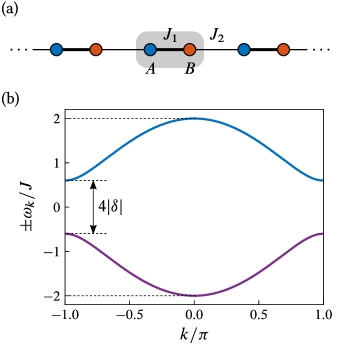
Figure 2.1: (a) Schematic drawing of the SSH model: a 1D lattice with two sites per unit cell (in gray), labelled $A$ and $B$, with alternating hopping amplitudes $J_{1}=J(1+\delta)$ and $J_{2}=J(1-\delta)$. (b) Upper and lower energy bands of the SSH model.

The SSH model has all three symmetries mentioned in previous paragraphs: time-reversal, charge-conjugation and chiral symmetry. Thus, according to the classification, it belongs to the BDI class, which in 1D supports distinct topological phases characterized by a $\mathbb{Z}$ topological invariant. To find this invariant, let us point out that chiral symmetry is represented in momentum space by the $z$-Pauli matrix $\sigma_{z}$, that is, $\sigma_{z}H_{k}\sigma_{z}=-H_{k}$. Expressing $H_{k}$ in the basis of Pauli matrices, $H_{k}=h_{0}(k)I+\mathbf{h}(k)\cdot\boldsymbol{\sigma}$, this symmetry constraint forces $h_{0}(k)=0$ and $h_{z}(k)=0$, so the vector $\mathbf{h}(k)$ lies on a plane. Also, the existence of a gap requires $\mathbf{h}(k)\neq 0$. Therefore, $\mathbf{h}(k)$ is a map from $S^{1}$ (the first Brillouin zone) to $\mathbb{R}^{2}\setminus\{0\}$. Such maps can be characterized by a topological invariant that only takes integer values: the winding number, $\mathcal{W}$, of the curve $\mathbf{h}(k)$ around the origin. Furthermore, as long as symmetries are preserved it is impossible to change the winding number of the curve without making it pass through the origin, in accordance with the fact that distinct topological phases are separated by phase transitions in which the gap closes.

The SSH model can be in two distinct phases: a topological phase with $\mathcal{W}=1$, for $J_{1}<J_{2}$ ($\delta<0$), or a trivial phase with $\mathcal{W}=0$, for $J_{1}>J_{2}$ ($\delta>0$). We remark that higher winding numbers can be achieved if longer-range hoppings are included [56, 57]. By the bulk-boundary correspondence, the value of $|\mathcal{W}|$ corresponds to the number of pairs of edge states supported by the system [58]. These states are exponentially localized at the edges of the chain and its energy is pinned on the middle of the band gap. In Fig. 2.2(a) we show the energy spectrum of a finite chain consisting of $N=10$ dimers. There, it can be seen how for $\delta<0$ the energies of two states detach from the bulk energy bands (shaded areas) and quickly converge to zero. By the energy spectrum, in Fig. 2.2(b), we show the amplitudes of the two midgap states for a particular value of $\delta<0$, proving that they are exponentially localized to the edges of the chain. To better understand the features of the energy spectrum and the edge states let us turn again to chiral symmetry. For systems defined on a lattice, we say that the system is bipartite if the lattice can be divided in two sublattices ($A$ and $B$) such that hopping processes only connect sites belonging to different sublattices. As it turns out, any bipartite lattice has chiral symmetry embodied in the transformation $c_{jA}\to c_{jA}$, $c_{jB}\to-c_{jB}$. Its action over a single-particle wavefunction is to reverse the sign of the amplitudes on one sublattice—hence, the name sublattice symmetry—which changes the sign of the Hamiltonian. This implies that the eigenvalues either come in pairs with opposite energies or have energy equal to zero and are also eigenvalues of the chiral symmetry operator. Note that the eigenstates in a pair have the same wavefunction, except for a change of the sign of the amplitudes in one sublattice. On the other hand, eigenstates with zero energy have support on a single sublattice. Edge states in the thermodynamic limit have zero energy, but in a finite system they hybridize forming symmetric and antisymmetric combinations which constitute a chiral symmetric pair with an energy splitting $\Delta\epsilon$ that decreases exponentially with increasing chain size, $\Delta\epsilon\propto e^{-N/\lambda}$.

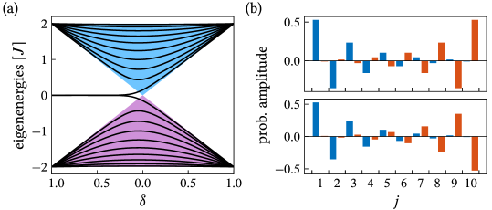
Figure 2.2: (a) Single-particle spectrum as a function of the dimerization constant for a finite chain with $N=10$ unit cells. The shaded areas correspond to the ranges of the energy bands in the thermodynamic limit (b) Edge states for the same chain at $\delta=-0.2$; blue (red) bars correspond to the amplitudes in sublattice $A$ ($B$)

For chains with an odd number of sites there must be an odd number of single-particle states precisely at zero energy due to chiral symmetry. Indeed, they support only one state at zero energy, exponentially localized on a single edge, with weight on just one sublattice. Note that in this case, changing the sign of $\delta$ amounts to inverting the chain spatially. Thus, depending on the sign of $\delta$ this edge state is localized on the left or right edge.

2.2.  Floquet theory

Floquet theory is concerned with the solution of periodic linear differential equations. In quantum mechanics, it is used to solve systems modelled by Hamiltonians with some explicit periodic time dependence, that is, solutions of the Schrödinger equation

$$i\partial_{t}\lvert\psi(t)\rangle=H(t)\lvert\psi(t)\rangle\,$$ (2.6)

with $H(t+T)=H(t)$ (here and throughout the text we work in units such that $\hbar=1$). For simplicity, we will just consider systems with a Hilbert space of finite dimension. Floquet’s theorem states that there is a fundamental set of solutions $\{\lvert\psi_{\alpha}(t)\rangle\}$ to this equation of the form $\lvert\psi_{\alpha}(t)\rangle=e^{-i\epsilon_{\alpha}t}\lvert\phi_{\alpha}(t)\rangle$, with $\epsilon_{\alpha}$ real and $\lvert\phi_{\alpha}(t)\rangle$ periodic with the same periodicity as the Hamiltonian, $\lvert\phi_{\alpha}(t+T)\rangle=\lvert\phi_{\alpha}(t)\rangle$ [59]. Therefore, any solution of Eq. (2.6) can be expanded as

$$\lvert\psi(t)\rangle=\mathop{{\sum}}_{\alpha}c_{\alpha}e^{-i\epsilon_{\alpha}t}\lvert\phi_{\alpha}(t)\rangle\,,$$ (2.7)

with time independent coefficients $c_{\alpha}$. In analogy with Bloch’s Theorem, $\epsilon_{\alpha}$ is called quasienergy and $\lvert\phi_{\alpha}(t)\rangle$ is called Floquet mode. Introducing $\lvert\psi_{\alpha}(t)\rangle$ in (2.6), we can see that Floquet modes satisfy the eigenvalue equation

$$\mathcal{H}\lvert\phi_{\alpha}\rangle\equiv\left(H-i\partial_{t}\right)\lvert\phi_{\alpha}\rangle=\epsilon_{\alpha}\lvert\phi_{\alpha}\rangle\,,$$ (2.8)

where $\mathcal{H}$ is the so-called Floquet operator, and it is Hermitian.

Equivalently, Floquet’s theorem states that for time-periodic systems the unitary time evolution operator can be factorized as

$$U(t_{2},t_{1})=\mathop{{\sum}}_{\alpha}e^{-i\epsilon_{\alpha}(t_{2}-t_{1})}\lvert\phi_{\alpha}(t_{2})\rangle\langle\phi_{\alpha}(t_{1})\rvert=e^{-iH_{\mathrm{eff}}(t_{2}-t_{1})}P(t_{2},t_{1})\,,$$ (2.9)

with $H_{\mathrm{eff}}=\sum_{\alpha}\epsilon_{\alpha}\lvert\phi_{\alpha}(t_{2})\rangle\langle\phi_{\alpha}(t_{2})\rvert$ being an effective time-independent Hamiltonian, and $P(t_{2},t_{1})=\sum_{\alpha}\lvert\phi_{\alpha}(t_{2})\rangle\langle\phi_{\alpha}(t_{1})\rvert$ a unitary operator, $T$-periodic in both of its arguments. The long-term dynamics is governed by $H_{\mathrm{eff}}$, wile the dynamics within a period, also known as the micromotion, is given by $P$. Note that there is a gauge freedom and we could also have written

$$U(t_{2},t_{1})=P^{\dagger}(t_{0},t_{2})e^{-iH_{\mathrm{eff}}(t_{2}-t_{1})}P(t_{0},t_{1})\,,$$ (2.10)

setting $H_{\mathrm{eff}}=\sum_{\alpha}\epsilon_{\alpha}\lvert\phi_{\alpha}(t_{0})\rangle\langle\phi_{\alpha}(t_{0})\rvert$. In some texts the micromotion operator is written as $P(t_{0},t)=e^{iK(t)}$, with $K(t)$ Hermitian and $T$-periodic, depending implicitly on the choice of $t_{0}$.

Floquet modes and quasienergies play a central role in the study of periodic systems. There are several ways to compute them. One can integrate numerically the dynamics of some states forming an orthonormal basis at $t_{1}=0$, obtaining $U(t,0)$ for $t\in[0,T]$. The eigenvalues of $U(T,0)$ are the complex phases $e^{-i\epsilon_{\alpha}T}$, with associated eigenvectors $\lvert\phi_{\alpha}(T)\rangle=\lvert\phi_{\alpha}(0)\rangle$. Their full time dependence can be reconstructed as $\lvert\phi_{\alpha}(t)\rangle=e^{i\epsilon_{\alpha}t}U(t,0)\lvert\phi_{\alpha}(0)\rangle$. Note that, since the quasienergies appear in a complex phase, they are defined modulo $2\pi/T=\omega$. Given a quasienergy $\epsilon_{\alpha}$, we can add to it a multiple of the frequency $\epsilon_{\alpha n}=\epsilon_{\alpha}+n\omega$ and the corresponding Floquet mode $\lvert\phi_{\alpha n}(t)\rangle=e^{in\omega t}\lvert\phi_{\alpha}(t)\rangle$ will also satisfy Eq. (2.8) with eigenvalue $\epsilon_{\alpha n}$. In fact any of these Floquet modes, $\lvert\phi_{\alpha n}(t)\rangle$, $n\in\mathbb{Z}$, yields the same solution to the Schrödinger equation. So, the quasienergy spectrum is periodic, much like quasimomentum in crystalline solids, and it suffices to consider the quasienergies within a range of width $\omega$.

Another procedure exploits the fact that that Floquet modes are periodic in time, so they can be expanded in Fourier series,

$$\lvert\phi_{\alpha}\rangle=\mathop{{\sum}}_{n}e^{-in\omega t}\lvert c_{\alpha n}\rangle\,,\quad\lvert c_{\alpha n}\rangle=\frac{1}{T}\int_{0}^{T}d\mkern-1.5mu{t}\,e^{in\omega t}\lvert\phi_{\alpha}(t)\rangle\,.$$ (2.11)

The time-independent vectors $\lvert c_{\alpha n}\rangle$ can themselves be expanded into some basis, $\{\lvert\beta\rangle\}$, of the system’s Hilbert space. Now, we can identify $e^{-in\omega t}\lvert\beta\rangle\equiv\lvert n\beta(t)\rangle$ as basis states of an enlarged Hilbert space built as the product of the system’s Hilbert space and the space of $T$-periodic functions [60]. We will denote the elements of this space as $\lvert\phi\rangle\!\rangle$, so that in “time representation” they are $\langle t\lvert\phi\rangle\!\rangle=\lvert\phi(t)\rangle$. An inner product can be defined in this enlarged space as the composition of the usual inner products in each of the constituent spaces

$$\langle\!\langle\phi|\phi^{\prime}\rangle\!\rangle=\frac{1}{T}\int_{0}^{T}d\mkern-1.5mu{t}\,\langle\phi(t)|\phi^{\prime}(t)\rangle\,.$$ (2.12)

With respect to this basis, the matrix elements of the Floquet operator are

$$\langle\!\langle n^{\prime}\beta^{\prime}\rvert\mathcal{H}\lvert n\beta\rangle\!\rangle =\frac{1}{T}\int_{0}^{T}d\mkern-1.5mu{t}\,e^{in^{\prime}\omega t}\langle\beta\rvert H(t)-i\partial_{t}\lvert\beta\rangle e^{-in\omega t}$$

$$=\langle\beta^{\prime}\rvert H_{n^{\prime}-n}\lvert\beta\rangle-n\omega\delta_{n^{\prime}n}\delta_{\beta^{\prime}\beta}\,,$$ (2.13)

where $H_{n^{\prime}-n}$ is the $(n^{\prime}-n)$th Fourier component of the Hamiltonian. Thereby, we have transformed a time-dependent problem into a time-independent one with an extra (infinite-dimensional) degree of freedom. This extra degree of freedom is directly related to the apparent redundancy of the Floquet modes mentioned earlier. Frequently, a time dependence in the Hamiltonian stems from the coupling to the modes of, e.g., a laser field in the semiclassical limit [61]. In this limit the basis states $\lvert\beta n\rangle\!\rangle$ can be interpreted as having a definite number of photons, and Floquet modes can be viewed as dressed states. Based on this analogy, the indices $(n^{\prime},n)$ in Eq. (2.13) are referred to as the photon indices. Furthermore, the matrix elements of $H_{m}$ are said to describe $m$-photon processes.

The benefit of this technique is that it allows the direct application of methods used for the diagonalization of time-independent Hamiltonians to compute quasienergies and Floquet modes. In the high frequency regime, blocks with different photon number are far apart in energy, and it makes sense to use perturbation theory to block diagonalize the Floquet operator [62, 63, 64]. This provides a series expansion of $H_{\mathrm{eff}}$ in powers of $\omega^{-1}$, known as the high-frequency expansion (HFE). In some situations, computing a few terms in this expansion is easier than computing the Floquet modes and quasienergies, and provides more physical insight. In section 3.2, we use this technique to investigate the dynamics of a pair of strongly-interacting fermions under the action of an ac field.

2.3.  Open quantum systems

Quantum mechanics has allowed us to explain many interesting phenomena at the cost of a more complicated description of fundamental particles and interactions. For example, the number of variables needed to describe the state of an ensemble of particles grows exponentially with the number of particles in the ensemble. This makes it very hard to analyze large systems involving many particles, or systems that interact with external, uncontrolled degrees of freedom. However, finding ways to tackle these problems is a necessity, since more often than not this is the situation we face in real experiments.

As opposed to closed quantum systems, open quantum systems are systems that interact with an environment, also called bath or reservoir, which is a collection of infinitely many degrees of freedom. Through this interaction the system exchanges information, energy and particles with the environment. As a result, dissipation and decoherence are introduced into the system [65]. The former is the phenomenon by which the system exchanges energy with the environment, eventually reaching thermal equilibrium with it, while the latter is the phenomenon by which coherent superpositions of states are lost over time. Below we summarize two distinct approaches to the study of open quantum systems.

2.3.1.  Master equations

A proper description of the system taking into account the effects of decoherence and dissipation is given by a density matrix, which besides pure states also includes statistical mixtures of them. The usual way to study this type of problems involves tracing out the bath degrees of freedom, obtaining a first order linear differential equation for the system’s reduced density matrix, the so-called master equation. There are different ways to do this depending on the regime and approximations that apply to the system under consideration [66].

We now proceed to show how to obtain a master equation, valid in the regime of weak system-bath coupling. The combination of system and bath is described as a whole by the Hamiltonian $H=H_{S}+H_{B}+H_{I}$, where $H_{S}$ and $H_{B}$ are the free Hamiltonians of system and bath respectively, and $H_{I}$ is the Hamiltonian that describes the interaction between them. We restrict the interaction to the case where $H_{I}$ is linear in both system and bath operators, $\{X_{j}\}$ and $\{B_{j}\}$ respectively, $H_{I}=\sum_{j}X_{j}\otimes B_{j}$. The entire system evolves according to the von-Neumann equation:

$$\dot{\tilde{\rho}}(t)=-i[\tilde{H_{I}}(t),\tilde{\rho}(t)]\,,$$ (2.14)

Here, $\rho$ is the full density matrix of the system plus the bath; the tilde over an operator denotes the interaction picture,

$$\tilde{O}(t)\equiv e^{i(H_{S}+H_{B})t}Oe^{-i(H_{S}+H_{B})t}\,,$$ (2.15)

where $O$ is the corresponding operator in the Schrödinger picture. Notice that at time $t=0$, both the Schrödinger and the interaction picture representations coincide. The integral form of Eq. (2.14) is

$$\tilde{\rho}(t)=\rho(0)-i\int_{0}^{t}d\mkern-1.5mu{s}\,[\tilde{H_{I}}(s),\tilde{\rho}(s)]\,.$$ (2.16)

Inserting this expression for $\rho(r)$ back in the right hand side of Eq. (2.14), tracing over the bath degrees of freedom, we get

$$\dot{\tilde{\rho_{S}}}(t)=-i\operatorname{tr}_{B}[\tilde{H_{I}}(t),\rho(0)]-\int_{0}^{t}d\mkern-1.5mu{s}\,\operatorname{tr}_{B}[\tilde{H_{I}}(t),[\tilde{H_{I}}(s),\tilde{\rho}(s)]]\,.$$ (2.17)

To obtain a closed equation for the reduced density matrix of the system, we need to make some approximations:

• Born approximation: We assume that at all times, the total density matrix can be factorized as $\rho(t)\approx\rho_{S}(t)\otimes\rho_{B}$. This amounts to neglect any entanglement between the system and the bath, which is justified if the coupling between them is small enough. Furthermore we will always consider a thermal state for the bath $\rho_{B}\propto e^{-\beta H_{B}}$.

• Markov approximation: We replace $\rho_{S}(s)$ by $\rho_{S}(t)$ in the integrand, such that the time evolution of the system only depends on its current state but not on its previous states. Furthermore, we let the lower integration bound go to $-\infty$ and make a change of variable $s=t-\tau$. This approximation is justified if the timescale in which the reservoir correlations decay is small compared to the timescale in which the system varies noticeably.

Last, if $\langle\tilde{B}_{j}(t)\rangle=0$, where we denote $\langle x\rangle\equiv\operatorname{tr}_{B}(x\rho_{B})$, as is the case in all the models presented in this thesis, we can neglect the first term, obtaining

$$\dot{\tilde{\rho_{S}}}(t)=-\int_{0}^{\infty}d\mkern-1.5mu{\tau}\,\operatorname{tr}_{B}[\tilde{H_{I}}(t),[\tilde{H_{I}}(t-\tau),\tilde{\rho_{S}}(t)\otimes\rho_{B}]]\,.$$ (2.18)

Transforming it back to the Schrödinger picture, we get

$$\begin{split}\dot{\rho_{S}}&=-i[H_{S},\rho_{S}]-\int_{0}^{\infty}d\mkern-1.5mu{\tau}\,\operatorname{tr}_{B}[H_{I},[\tilde{H_{I}}(-\tau),\rho_{S}\otimes\rho_{B}]]\\ &\equiv-i[H_{S},\rho_{S}]+\mathcal{L}[\rho_{S}]\,,\end{split}$$ (2.19)

where the first term accounts for the coherent unitary dynamics, whereas the second includes dissipation and decoherence.

This equation, known in the literature as the Bloch-Redfield master equation [67], is the one we will use for studying the decay of doublons in noisy environments, see section 3.3 and appendix 3.B. Note that this equation does not necessarily preserve the positivity of the density matrix. One has to perform a further rotating-wave approximation, which involves averaging over the rapidly oscillating terms in Eq. (2.18) to obtain an equation that does preserve it, i.e., one that can be put in Lindblad form [66]. This other equation, known as the quantum optical master equation in some contexts, is the one we will use for studying the dynamics of quantum emitters coupled to a topological bath , see chapter 4 and appendix 4.B.

2.3.2.  Resolvent formalism

Quite often in quantum physics we want to know what happens to a particular system of interest (e.g. a qubit or atom) when coupling it to an external driving, or a bath. The coupling may induce transitions between the bare eigenstates of the system, whose probability can be computed exactly in some cases with resolvent operator techniques [68, 69].

Let us consider a system with free Hamiltonian $H_{0}$, perturbed such that the actual Hamiltonian of the system is $H=H_{0}+V$. The time evolution operator satisfies

$$i\partial_{t}U(t,t_{0})=HU(t,t_{0})\,.$$ (2.20)

We can split the time evolution operator into two operators $G^{\pm}(t,t_{0})$ that evolve the state of the system at time $t=t_{0}$ forwards and backwards in time respectively,

$$G^{\pm}(t,t_{0})=\pm U(t,t_{0})\Theta\left(\pm(t-t_{0})\right)\,.$$ (2.21)

Here, $\Theta(t)$ denotes Heaviside’s step function. Differentiating Eq. (2.21) we can see that they satisfy the same equation,

$$\left(i\partial_{t}-H\right)G^{\pm}(t,t_{0})=i\delta(t-t_{0})\,.$$ (2.22)

They are usually referred to as the retarded (“$+$”) and advanced (“$-$”) Green’s functions or propagators. For a time-independent system $G^{\pm}(t,t_{0})$ depends only on $\tau=t-t_{0}$. Let us now introduce their Fourier transform

$$G^{\pm}(\tau,0)=-\frac{1}{2\pi i}\int_{-\infty}^{\infty}d\mkern-2.0muE\,e^{-iE\tau}G^{\pm}(E)\,,$$ (2.23)

$$G^{\pm}(E)=\frac{1}{i}\int_{-\infty}^{\infty}d\mkern-1.5mu{\tau}\,e^{iE\tau}G^{\pm}(\tau,0)\,,$$ (2.24)

Substituting $G^{+}(\tau,0)=e^{-iH\tau}\Theta(\tau)$ in Eq. (2.24) we find

$$G^{+}(E) =\frac{1}{i}\int_{0}^{\infty}d\mkern-1.5mu{\tau}\,e^{i(E-H)\tau}=\lim_{\eta\to 0^{+}}\frac{1}{i}\int_{0}^{\infty}d\mkern-1.5mu{\tau}\,e^{i(E-H+i\eta)\tau}$$

$$=\lim_{\eta\to 0^{+}}\frac{1}{E-H+i\eta}\,,$$ (2.25)

and similarly,

$$G^{-}(E)=\lim_{\eta\to 0^{+}}\frac{1}{E-H-i\eta}\,.$$ (2.26)

These expressions suggest the definition of the operator

$$G(z)=\frac{1}{z-H}\,,$$ (2.27)

which is a function of a complex variable $z$, such that $G^{\pm}(E)=G(E\pm i0^{+})$. $G(z)$ is called the resolvent of the Hamiltonian $H$.

From the definition (2.21), it is clear that the transition amplitudes from an initial state $\lvert\alpha\rangle$ to a final state $\lvert\beta\rangle$ after a period $\tau$ can be computed as

$$\langle\beta\rvert U(\tau)\lvert\alpha\rangle=-\frac{1}{2\pi i}\int_{-\infty}^{\infty}d\mkern-2.0muE\,e^{-iE\tau}\langle\beta\rvert G(E+i0^{+})\lvert\alpha\rangle\,.$$ (2.28)

Thus, the analytical properties of the matrix elements of the resolvent play a crucial role in determining the dynamics of the system. It can be shown that the matrix elements of $G(z)$ are analytic in the whole complex plane except for the real axis, where they have poles and branch cuts at the discrete and continuous spectrum of $H$ respectively. Furthermore, it is possible to continue analytically $G(z)$ bridging the cuts in the real axis, exploring other Riemann sheets of the function, where it may no longer be analytic and may contain poles with a nonzero imaginary part, the so-called unstable poles.

We will now see how to obtain explicit formulas for the relevant matrix elements of the resolvent. Suppose we want to know what happens to the states of a particular subspace spanned by $\{\lvert\alpha\rangle\}$, which are eigenstates of $H_{0}$. Let us denote the projector onto that subspace as $P=\sum_{\alpha}\lvert\alpha\rangle\langle\alpha\rvert$, and the projector on the complementary subspace as $Q=1-P$. Then, from the defining equation of the resolvent $\left(z-H\right)G=1$, multiplying it from the right by $P$, and from the left by $P$ and $Q$, we get the equations

$$P(z-H)P\left[PGP\right]-PVQ\left[QGP\right]=P\,,$$ (2.29)

$$-QVP\left[PGP\right]+Q(z-H)Q\left[QGP\right]=0\,.$$ (2.30)

Solving for $QGP$ in Eq. (2.30)

$$QGP=\frac{Q}{z-QH_{0}Q-QVQ}VPGP\,,$$ (2.31)

and substituting back in Eq. (2.29), we obtain

$$P\left[z-H_{0}-V-V\frac{Q}{z-QH_{0}Q-QVQ}V\right]PGP=P\,.$$ (2.32)

Introducing the operator

$$R(z)=V+V\frac{Q}{z-QH_{0}Q-QVQ}V\,,$$ (2.33)

which is known as the level-shift operator, we can express

$$PG(z)P=\frac{P}{z-PH_{0}P-PR(z)P}\,.$$ (2.34)

From Eq. (2.31) we can now obtain

$$QG(z)P=\frac{Q}{z-QH_{0}Q-QVQ}V\frac{P}{z-PH_{0}P-PR(z)P}.$$ (2.35)

In section 4.1 and appendix 4.A we use these formulas for computing the survival probability amplitude of the excited state of one and two quantum emitters.

3Doublon dynamics

Recent experimental advances have provided reliable and tunable setups to test and explore the quantum mechanical world. Paradigmatic examples are ultracold atoms trapped in optical lattices [22, 23], quantum dots [34, 35, 70, 71], and photonic crystals [72, 73, 74, 75]. In these setups, quantum coherence is responsible for many exotic phenomena, in particular, the transfer of quantum information between different locations, a process known as quantum state transfer. Even particles themselves, which may carry quantum information encoded in their internal degrees of freedom, can be transferred in a controlled manner in these setups. Given its importance in quantum information processing applications, many theoretical and experimental works have studied these processes in recent years [76, 77, 78, 79, 80].

Floquet engineering, that is, the use of periodic drivings in order to modify the properties of a system, has become an essential technique in the cold-atom toolbox, which has enabled the simulation of some topological models [30, 31, 32]. However, most of the studies carried out so far utilize this technique aimed at the single-particle level. In this chapter we investigate the dynamics of two strongly interacting fermions bound together, forming what is termed a “doublon”, under the action of periodic drivings. We show how to harness the topological properties of different lattices to transfer doublons [81], and demonstrate a phenomenon by which the driving confines doublon dynamics to a particular sublattice [82]. Afterwards, we address the question whether doublons can be observed in noisy systems such as quantum dot arrays [83].

3.1.  What are doublons?

An ubiquitous model in the field of Condensed Matter is the Hubbard model. Despite its seeming simplicity, it captures a great variety of phenomena ranging from metallic behavior to insulators, magnetism and superconductivity. The Hamiltonian of this model consists of two contributions: a hopping term $H_{J}$ that corresponds to the kinetic energy of particles moving in a lattice, and an on-site interaction term $H_{U}$ that corresponds to the interaction between particles occupying the same lattice site. For spin-1/2 fermions, this Hamiltonian can be written as

$$H=-\mathop{{\sum}}_{i,\,j,\,\sigma}J_{ij}c^{\dagger}_{i\sigma}c_{j\sigma}+U\mathop{{\sum}}_{i}n_{i{\uparrow}}n_{i{\downarrow}}\equiv H_{J}+H_{U}\,.$$ (3.1)

Here, $c_{i\sigma}$ annihilates a fermion with spin $\sigma\in\{{\uparrow},{\downarrow}\}$ at site $i$, and $n_{i\sigma}=c^{\dagger}_{i\sigma}c_{i\sigma}$ is the usual number operator. $J_{ij}$ is the, possibly complex, hopping amplitude between sites $i$ and $j$ (Hermiticity of $H$ requires $J_{ij}=J_{ji}^{*}$). The interaction strength $U$ corresponds to the energy cost of the double occupancy.

As we shall see, in the strongly interacting limit of the Hubbard model ($U\gg\lvert J_{ij}\rvert$) particles occupying the same lattice site can bind together, even for repulsive interactions. This happens due to energy conservation, and the fact that, in a lattice, the maximum kinetic energy a particle can have is limited to the width of the energy bands. Therefore, an initial state where the particles occupy the same site cannot decay to a state where the particles are separated, since they would not have enough kinetic energy on their own to compensate for the large interaction energy. In principle, both bosons [84, 85, 86] and fermions [87, 88] can form such $N$-particle bound states. While the former allow for any occupation number, for fermions with spin $s$ the occupation of one site is restricted to at most $2s+1$ particles. In particular, two spin-1/2 fermions may be in a singlet spin configuration on the same lattice site and form a doublon. Over the last years they have been investigated experimentally, mostly with cold atoms in optical lattices [89, 90, 91, 92, 93].

The Hilbert space of two particles in a singlet configuration is spanned by two types of states: single-occupancy states

$$\frac{1}{\sqrt{2}}\left(c^{\dagger}_{i{\uparrow}}c^{\dagger}_{j{\downarrow}}-c^{\dagger}_{i{\downarrow}}c^{\dagger}_{j{\uparrow}}\right)\lvert 0\rangle\,,\quad 1\leq i<j\leq N\,,$$ (3.2)

and double-occupancy states, also known as doublons,

$$c^{\dagger}_{j{\uparrow}}c^{\dagger}_{j{\downarrow}}\lvert 0\rangle\,,\quad j=1,\dots,N\,.$$ (3.3)

Both are eigenstates of $H_{U}$ with eigenvalues $0$ and $U$ respectively. The hopping term couples both types of states, so that they no longer are eigenstates of the full Hamiltonian. However, for sufficiently large values of $U$ the eigenstates also discern in two groups, namely, $N(N-1)/2$ states with energies $|\epsilon_{n}|\lesssim 4J$, which have a large overlap with the single-occupancy states, and $N$ states with energies $|\epsilon_{n}|\simeq U$, which have a large overlap with the doublon states. We will refer to the span of the former as the low-energy subspace (they are also referred to as scattering eigenstates), and the span of the latter as the high-energy subspace (also known as two-particle bound states). This distinction can be clearly appreciated in Fig. 3.1. In this regime, a state initially having a high double occupancy will remain like that as it evolves in time. In this sense, we can say that the total double occupancy is an approximate conserved quantity in the strongly-interacting regime.

Treating the tunneling as a perturbation it is possible to obtain an effective Hamiltonian for the high-energy subspace [94]. The method, which goes by the name of Schrieffer-Wolff transformation [95], provides a unitary transformation that block-diagonalizes the Hamiltonian perturbatively in blocks of states with different number of doubly occupied sites. To achieve this, we first split the kinetic term into hoppings that increase, decrease, and leave unaltered the double occupancy, $H_{J}=H^{+}_{J}+H^{-}_{J}+H^{0}_{J}$, where

$$H^{+}_{J}=-\mathop{{\sum}}_{i,\,j,\,\sigma}J_{ij}n_{i\bar{\sigma}}c^{\dagger}_{i\sigma}c_{j\sigma}h_{j\bar{\sigma}}\,,$$ (3.4)

$$H^{-}_{J}=-\mathop{{\sum}}_{i,\,j,\,\sigma}J_{ij}h_{i\bar{\sigma}}c^{\dagger}_{i\sigma}c_{j\sigma}n_{j\bar{\sigma}}\,,$$ (3.5)

$$H^{0}_{J}=-\mathop{{\sum}}_{i,\,j,\,\sigma}J_{ij}\left(n_{i\bar{\sigma}}c^{\dagger}_{i\sigma}c_{j\sigma}n_{j\bar{\sigma}}+h_{i\bar{\sigma}}c^{\dagger}_{i\sigma}c_{j\sigma}h_{j\bar{\sigma}}\right)\,.$$ (3.6)

In these equations $\bar{\sigma}$ denotes the opposite value of $\sigma$ and $h_{i\sigma}\equiv 1-n_{i\sigma}$. The transformation of $H$ by any unitary $e^{iS}$ ($S^{\dagger}=S$) can be computed as

$$\tilde{H}=e^{iS}He^{-iS}=H+\frac{[iS,H]}{1!}+\frac{[iS,[iS,H]]}{2!}+\cdots\,.$$ (3.7)

Noting that $\left[H_{U},H^{\alpha}_{J}\right]=\alpha UH^{\alpha}_{J}$, $\alpha\in\{\pm,0\}$, one can readily see that in order to remove the terms that couple the two sectors at zeroth order, $H^{\pm}_{J}$, one has to choose $iS={\left(H^{+}_{J}-H^{-}_{J}\right)/U}$. Then,

$$\tilde{H}=H^{0}_{J}+H_{U}+\frac{\left[H^{+}_{J},H^{-}_{J}\right]+\left[H^{0}_{J},H^{-}_{J}\right]+\left[H^{+}_{J},H^{-}_{J}\right]}{U}+O\left(U^{-2}\right)\,.$$ (3.8)

Keeping terms up to order $U^{-1}$ that act non-trivially on doublon states, we obtain the following effective Hamiltonian for doublons

$$H_{\mathrm{eff}}=H_{U}+\frac{1}{U}H^{+}_{J}H^{-}_{J}\,.$$ (3.9)

Since we are concerned with states with no singly occupied sites, in $H^{+}_{J}H^{-}_{J}$ we have to consider just those hopping processes where a doublon splits and then recombines again to the same site or to an adjacent site,

$$H^{+}_{J}H^{-}_{J}\stackrel{{\scriptstyle*}}{{=}}\mathop{{\sum}}_{i,\,j,\,\sigma}\lvert J_{ij}\rvert^{2}n_{i\bar{\sigma}}c^{\dagger}_{i\sigma}c_{j\sigma}h_{j\bar{\sigma}}h_{j\bar{\sigma}}c^{\dagger}_{j\sigma}c_{i\sigma}n_{i\bar{\sigma}}+\mathop{{\sum}}_{i,\,j,\,\sigma}J_{ij}^{2}n_{i\bar{\sigma}}c^{\dagger}_{i\sigma}c_{j\sigma}h_{j\bar{\sigma}}h_{i\sigma}c^{\dagger}_{i\bar{\sigma}}c_{j\bar{\sigma}}n_{j\sigma}\,.$$ (3.10)

The asterisk on top of the equal sign denotes equality when restricted to the doublon subspace. The terms in the first sum can be rewritten as

$$n_{i\bar{\sigma}}c^{\dagger}_{i\sigma}c_{j\sigma}h_{j\bar{\sigma}}h_{j\bar{\sigma}}c^{\dagger}_{j\sigma}c_{i\sigma}n_{i\bar{\sigma}}=n_{i\bar{\sigma}}n_{i\sigma}-n_{i\bar{\sigma}}n_{i\sigma}n_{j\bar{\sigma}}n_{j\sigma}\,,\quad i\neq j\,.$$ (3.11)

Here, we have used the fact that for a doublon state, if a site is occupied it has to be double occupied, i.e., $n_{i\sigma}\stackrel{{\scriptstyle*}}{{=}}n_{i\sigma}n_{i\bar{\sigma}}\stackrel{{\scriptstyle*}}{{=}}n_{i\bar{\sigma}}$. As for the terms in the second sum,

$$n_{i\bar{\sigma}}c^{\dagger}_{i\sigma}c_{j\sigma}h_{j\bar{\sigma}}h_{i\sigma}c^{\dagger}_{i\bar{\sigma}}c_{j\bar{\sigma}}n_{j\sigma}=c^{\dagger}_{i\bar{\sigma}}c^{\dagger}_{i\sigma}c_{j\sigma}c_{j\bar{\sigma}}\,,\quad i\neq j\,.$$ (3.12)

Finally, using doublon creation and annihilation operators, $d^{\dagger}_{i}=c^{\dagger}_{i{\uparrow}}c^{\dagger}_{i{\downarrow}}$ and $d_{i}=c_{i{\downarrow}}c_{i{\uparrow}}$, the effective Hamiltonian for doublons can be written as

$$H_{\mathrm{eff}}=\mathop{{\sum}}_{i,\,j}\frac{2J_{ij}^{2}}{U}d^{\dagger}_{i}d_{j}+\mathop{{\sum}}_{i}\mu_{i}d^{\dagger}_{i}d_{i}-\mathop{{\sum}}_{i,\,j}\frac{2\lvert J_{ij}\rvert^{2}}{U}d^{\dagger}_{i}d_{i}d^{\dagger}_{j}d_{j}\,,$$ (3.13)

with $\mu_{i}=U+\sum_{j}2\lvert J_{ij}\rvert^{2}/U$. The first term corresponds to an effective hopping for doublons, the second to an effective on-site chemical potential, and the third to an attractive interaction between doublons.

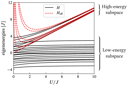
Figure 3.1: Energy spectrum of $H$ and $H_{\mathrm{eff}}$ for two spin-1/2 fermions forming a singlet in the SSH-Hubbard model (chain with $N=3$ dimers and $\delta=-0.2$, see next section) as a function of the interaction strength. For large interactions, the effective Hamiltonian correctly reproduces the eigenenergies of the high-energy subspace.

We remark that for a 1D lattice with homogeneous nearest-neighbor hoppings, the two-body spectrum can be computed exactly with Bethe Ansatz techniques [96].

In appendix 3.A we derive an effective Hamiltonian for doublons including also the effect of an external periodic driving.

3.2.  Doublon dynamics in 1D and 2D lattices

After understanding what doublons are, and what makes them stable quasiparticles, we are now in a good position to discuss their dynamics. In this section we show how the interplay between topology, interactions, and driving, leads to surprising effects that constrain the motion of doublons.

3.2.1.  Dynamics in the SSH chain

Interestingly, the topological properties of the SSH model can be harnessed to produce the transfer of non-interacting particles between the ends of a finite chain, without them occupying the intervening sites. Key to this process is the presence of edge states. Let us recall their properties. A finite dimer chain supports two edge states $\lvert\mathrm{ES}_{\pm}\rangle$, with energies $\pm\epsilon/2$, when it is in the topological phase ($\delta<0$). They are well separated energetically from the rest of (bulk) states, and there is a small energy splitting between them that decreases exponentially with increasing chain size, $\epsilon\propto e^{-N/\lambda}$. Each of them is exponentially localized on both edges of the chain, and they are even and odd under space inversion; thus, they can be regarded as a non-local two level system. As a consequence, a particle in a superposition of both edge states will oscillate between the ends of the chain as it evolves in time. For example, if the particle is initially on the first site of the chain $\lvert\psi(0)\rangle=\lvert 1\rangle\simeq\left(\lvert\mathrm{ES}_{+}\rangle+\lvert\mathrm{ES}_{-}\rangle\right)/\sqrt{2}$, the probability to find it on the last site of the chain $\lvert 2N\rangle\simeq\left(\lvert\mathrm{ES}_{+}\rangle-\lvert\mathrm{ES}_{-}\rangle\right)/\sqrt{2}$ is

$$\lvert\langle 2N|\psi(t)\rangle\rvert^{2}=\frac{1}{4}\left\lvert e^{-i\epsilon t/2}-e^{i\epsilon t/2}\right\rvert^{2}=\frac{1-\cos(\epsilon t)}{2}\,,$$ (3.14)

thus, in a time period $T_{0}=\pi/\epsilon$ the particle will be transferred with certainty to the other end of the chain.

We want to know how interaction between particles affects this process, and see whether the controlled transfer of doublons is possible. The Hamiltonian of the system corresponds to Eq. (3.1) with

$$J_{ij}=\begin{cases}J\left[1+\delta(-1)^{\max(i,j)}\right]\,,&\lvert i-j\rvert=1\\ 0\,,&\text{otherwise}\end{cases}\,.$$ (3.15)

This is just a different way to express $H_{\mathrm{SSH}}$ [Eq. (2.1) in section 2.1] including the spin degree of freedom and the on-site interaction between particles. We will refer to this model as the SSH-Hubbard model.

In Fig. 3.2 (top row) we plot the dynamics of a doublon starting on the first site of a small chain. As can be observed, the edge-to-edge oscillations are lost in the strongly-interacting regime. We can understand why looking at the effective Hamiltonian for doublons

$$H_{\mathrm{eff}}=\mathop{{\sum}}_{j}\left(J^{\mathrm{eff}}_{1}d^{\dagger}_{2j}d_{2j-1}+J^{\mathrm{eff}}_{2}d^{\dagger}_{2j+1}d_{2j}+\mathrm{H.c.}\right)+\mathop{{\sum}}_{j}\mu_{j}d^{\dagger}_{j}d_{j}\,,$$ (3.16)

which can be obtained directly from Eq. (3.13), neglecting the interaction between doublons, since we are considering just one of them. The effective hopping amplitudes are $J^{\mathrm{eff}}_{1}=2J^{2}(1+\delta)^{2}/U$ and $J^{\mathrm{eff}}_{2}=2J^{2}(1-\delta)^{2}/U$. Importantly, the effective local chemical potential $\mu_{j}$ is different for the ending sites, as they have one fewer neighbor,

$$\mu_{j}=\begin{cases}\mu_{\mathrm{bulk}}=J^{\mathrm{eff}}_{1}+J^{\mathrm{eff}}_{2}+U\,,&2\leq j\leq 2N-1\\ \mu_{\mathrm{edge}}=J^{\mathrm{eff}}_{1}+U\,,&j=1,2N\end{cases}\,.$$ (3.17)

This chemical potential difference at the edges spoils the chiral symmetry of the model, and is able to shift the energy of the edge states that appear in the topological phase of the unperturbed SSH model. In fact, for the particular value $\Delta\mu\equiv\mu_{\mathrm{bulk}}-\mu_{\mathrm{edge}}=J^{\mathrm{eff}}_{2}$, they completely merge into the bulk bands, see Fig. 3.2 (top row). This explains why the mechanism that produces the edge-to-edge oscillations in the single particle case does not apply directly to the doublon case.

We can now think of different ways to restore the edge states in order to produce the transfer of doublons. One possibility is is to add a local potential at the edges of the chain so as to compensate for the difference in chemical potential,

$$H=H_{J}+H_{U}+V_{\mathrm{gate}}\mathop{{\sum}}_{\sigma}\left(n_{1\sigma}+n_{2N\sigma}\right)\,,$$ (3.18)

with $V_{\mathrm{gate}}=J^{2}(1-\delta)^{2}/U$. The resulting effective Hamiltonian has a homogeneous chemical potential $\mu_{j}=\mu_{\mathrm{gate}}$ for all $j$, and is formally identical to that of the SSH model. Indeed, this produces the desired dynamics, see Fig. 3.2 (middle row). Another possibility is to take advantage of this chemical potential difference, which can localize states on the edges of the chain of the Shockley type. This requires the hopping amplitudes to be smaller than $\Delta\mu$. Usually this is not the case, however there is an efficient way to induce such states by driving the system with a high-frequency ac field. The ac field renormalizes the hoppings, which become smaller than in the undriven case [24, 97, 25]. This cannot be achieved, for example, by simply reducing the hoppings $J_{1}$ and $J_{2}$ by hand, since this will also affect the effective chemical potential which still will be of the same order of $J^{\mathrm{eff}}_{1}$ and $J^{\mathrm{eff}}_{2}$. To model the ac field we add a periodically oscillating potential that rises linearly along the lattice,

$$H(t)=H_{J}+H_{U}+E\cos(\omega t)\mathop{{\sum}}_{j}x_{j}\left(n_{j{\uparrow}}+n_{j{\downarrow}}\right)\,.$$ (3.19)

Here, $E$ and $\omega$ are the amplitude and frequency of the driving, and $x_{j}$ is the spatial coordinate along the chain. The geometry of the chain is determined by the lattice constant, which we set as the unit of distance, and the intracell distance $b\in[0,1]$, such that $x_{j}=\lfloor(j-1)/2\rfloor+b{(j-1\mod 2)}$. Since the Hamiltonian is periodic in time we can apply Floquet theory and obtain a time-independent effective Hamiltonian in the high-frequency regime, see appendix 3.A. As it turns out, when the leading energy scale is that of the of the interaction between particles, the effective Hamiltonian for doublons is the same as the one in Eq. (3.16) with renormalized hopping amplitudes

$$J^{\mathrm{eff}}_{1}=\mathcal{J}_{0}\left(\frac{2Eb}{\omega}\right)\frac{2J^{2}(1+\delta)^{2}}{U}\,,$$ (3.20)

$$J^{\mathrm{eff}}_{2}=\mathcal{J}_{0}\left(\frac{2E(1-b)}{\omega}\right)\frac{2J^{2}(1-\delta)^{2}}{U}\,,$$ (3.21)

where $\mathcal{J}_{0}$ denotes the zeroth order Bessel function of the first kind. The factor $2$ in the argument of $\mathcal{J}_{0}$ comes from the doublon’s twofold electric charge. We show the effect of this renormalization in Fig. 3.2 (bottom row); as the effective tunneling reduces in magnitude the bulk bands become narrower, and two Shockley edge states are pulled from the bottom of the lower band. The geometry, which so far did not played any role, now becomes important in this renormalization of the hoppings. The simplest case is for $b=1/2$, in which both hoppings are renormalized by the same factor. We remark that the on-site effective chemical potential, being a local operator, commutes with the periodic driving potential, and so it is not renormalized.

This approach has the peculiarity that it only relies on the $\Delta\mu$ produced by the interaction, and not on the topology of the chain. Thus, it can be used to produce the transfer of doublons in normal chains with an odd number of sites, see Fig. 3.2 (bottom row), contrary to the static approach. Notice that the high-frequency effective Hamiltonian preserves space inversion symmetry, which guarantees that the Shockley edge states hybridize forming even and odd combinations under space inversion, just like topological edge states do. However, Shockley edge states lack the protection against certain types of disorder, such as off-diagonal disorder (see section 4.1.1), that topological edge states have.

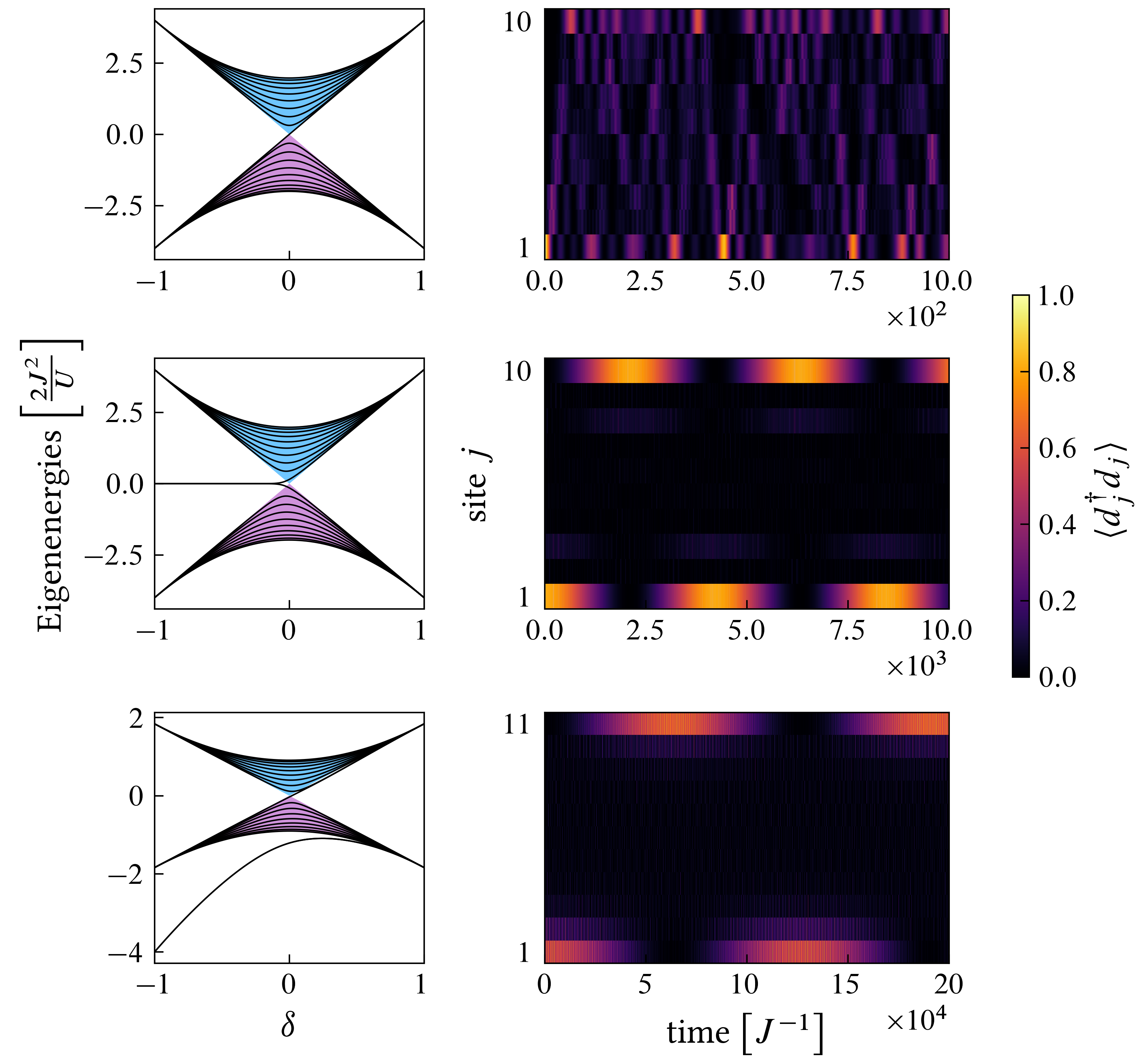
Figure 3.2: Spectrum of the effective Hamiltonian (left), and associated doublon dynamics (right), computed numerically solving the Schrödinger equation in the two-particle singlet subspace. In all the cases shown, a doublon is initially on the 1st site of the lattice. Case without any external influence (top row). The spectrum shows the absence of edge states for any value of $\delta$. The parameters for the dynamics are: $\delta=-0.3$, $U=10J$ and $N=5$. Case with a compensating local potential $V_{\mathrm{gate}}$ on the ending sites of the chain (middle row). A pair of topological edge states appears for negative values of $\delta$. The parameters for the dynamics are the same as in the previous case. Case with an external ac-field with parameters: $E=3.2J$, $\omega=2J$ and $b=1/2$ (bottom row). The spectrum shows a pair of Shockley edge states that separate from the bottom of the lower band. The dynamics is for a chain with $11$ sites, $\delta=0$, and $U=16J$.

Last, we can combine both approaches, restoring the symmetries of the SSH model, and being able to modify the system’s topology with the ac field, provided $b\neq 1/2$ [98]. In Fig. 3.3 we compare the exact quasienergies of the doublon states with the quasienergies given by the effective Hamiltonian. Both agree as long as photon-resonance effects are negligible, i.e., $E\lesssim U$ (see appendix 3.A). For field parameters such that $\lvert J^{\mathrm{eff}}_{1}\rvert<\lvert J^{\mathrm{eff}}_{2}\rvert$, the system supports a pair of topological edge states, which allow for the transfer of doublons.

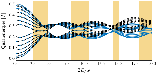
Figure 3.3: Quasienergy spectrum for a chain with a compensating local potential $V_{\mathrm{gate}}$ and an external ac field, as a function of the ac field amplitude. The parameters are $\delta=0.1$, $N=7$, $U=16J$, $b=0.6$, and $\omega=2J$. Exact quasienergies (dots) have been obtained diagonalizing the time evolution operator for one period. We only show the quasienergies corresponding to the $2N$ Floquet modes with largest total double occupancy. The lines correspond to the approximate quasienergies given by the effective Hamiltonian. Shaded areas mark the regions where the system is in the non-trivial phase, according to the values of $\lvert J^{\mathrm{eff}}_{1}\rvert$ and $\lvert J^{\mathrm{eff}}_{2}\rvert$.

3.2.2.  Dynamics in the $\mathcal{T}_{3}$ and Lieb lattices

We will now analyze the consequences of the effective local chemical potential on the doublon dynamics in 2D lattices. We will consider lattices with homogeneous hopping amplitudes threaded by a static magnetic flux in the presence of a circularly polarized ac field. They are modelled by the Hamiltonian

$$H(t)=-J\mathop{{\sum}}_{\langle i,j\rangle,\,\sigma}e^{i\phi_{ij}}c^{\dagger}_{i\sigma}c_{j\sigma}+U\mathop{{\sum}}_{j}n_{j{\uparrow}}n_{j{\downarrow}}+\mathop{{\sum}}_{j,\,\sigma}V_{j}(t)n_{j\sigma}\,,$$ (3.22)

with $V_{j}(t)=x_{j}E\cos(\omega t)+y_{j}E\sin(\omega t)$, where $(x_{j},y_{j})\equiv\mathbf{r}_{j}$ are the coordinates of site $j$. The sum in the hopping term runs over each oriented pair of nearest-neighbor sites. The magnetic flux induces complex phases in the hoppings such that the sum of the phases around a closed loop equals $2\pi\Phi/\Phi_{0}$, where $\Phi$ is the total flux threading the loop and $\Phi_{0}$ is the magnetic flux quantum.

The effective Hamiltonian for doublons generalizes in a straightforward manner for 2D lattices (see appendix 3.A),

$$H_{\mathrm{eff}}=J_{\mathrm{eff}}\mathop{{\sum}}_{\langle i,j\rangle}e^{i2\phi_{ij}}d^{\dagger}_{i}d_{j}+\mathop{{\sum}}_{j}\mu_{j}d^{\dagger}_{j}d_{j}\,,$$ (3.23)

with effective hopping and chemical potentials

$$J_{\mathrm{eff}}=\frac{2J^{2}}{U}\mathcal{J}_{0}\left(\frac{2Ea}{\omega}\right)\,,\quad\mu_{j}=\frac{2J^{2}}{U}z_{j}\,,$$ (3.24)

where $z_{j}$ is the coordination number (the number of nearest neighbors) of site $j$. In this effective Hamiltonian we have neglected again interaction terms, since we are considering just one doublon. Importantly, the hopping renormalization is isotropic because the ac field polarization is circular and all neighboring sites are the same distance apart; $\lvert\mathbf{r}_{i}-\mathbf{r}_{j}\rvert=a$ for all neighboring $i$ and $j$.

As we can see, the ac driving allows us to independently tune the effective hopping amplitude with respect to the effective local chemical potential. This has a big impact on the dynamics of doublons in lattices that can be divided into sublattices with different coordination numbers, such as the Lieb lattice, and the $\mathcal{T}_{3}$ lattice, shown in Fig. 3.4. As can be seen in the dynamics, the doublon moves mostly through sites with the same coordination number, an effect we have termed sublattice dynamics.

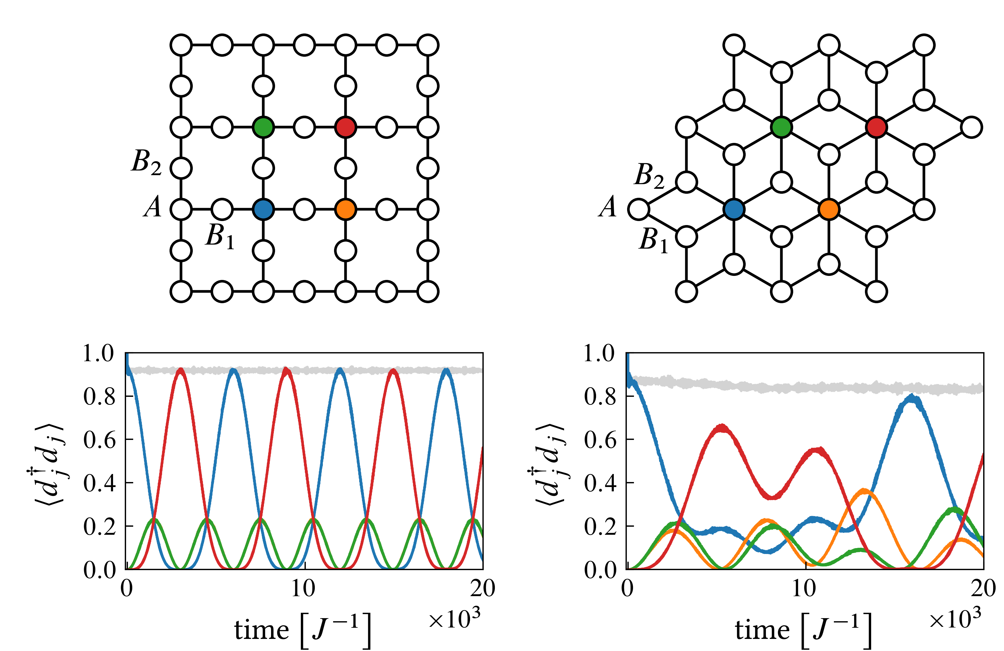
Figure 3.4: Doublon dynamics on a finite piece of a Lieb lattice (a) and a $\mathcal{T}_{3}$ lattice (b). In both cases the doublon is initially on the blue dot. Parameters: $\Phi=0$, $U=16J$, $\omega=2J$, and $E=4.8J$ (a), $E=4.2J$ (b). The grey line is the sum of the double occupancy on the four colored sites. In the Lieb lattice, the double occupancy on the green and yellow sites is the same. The dynamics have been obtained solving numerically the time-dependent Schrödinger equation in the two-particle singlet subspace.

To understand why, it is useful to look at the effective Hamiltonian in momentum representation, which in the absence of an external magnetic flux adopts the same form for both lattices $H_{\mathrm{eff}}=\sum_{\mathbf{k}}V^{\dagger}_{\mathbf{k}}H_{\mathbf{k}}V_{\mathbf{k}}$, with

$$H_{\mathbf{k}}=\begin{pmatrix}\Delta\mu&f_{1}(\mathbf{k})&f_{2}(\mathbf{k})\\ f^{*}_{1}(\mathbf{k})&0&0\\ f^{*}_{2}(\mathbf{k})&0&0\end{pmatrix}\,,\quad V_{\mathbf{k}}=\begin{pmatrix}d_{A\mathbf{k}}\\ d_{B_{1}\mathbf{k}}\\ d_{B_{2}\mathbf{k}}\end{pmatrix}\,.$$ (3.25)

Here, $d_{\alpha\mathbf{k}}$ is the annihilation operator of a doublon with momentum $\mathbf{k}$ in sublattice $\alpha\in\{A,B_{1},B_{2}\}$. The eigenenergies and eigenstates are as follows:

$$\epsilon^{0}_{\mathbf{k}}=0\,,\quad\epsilon^{\pm}_{\mathbf{k}}=\frac{1}{2}\left[\Delta\mu\pm\sqrt{4\lvert f_{1}(\mathbf{k})\rvert^{2}+4\lvert f_{2}(\mathbf{k})\rvert^{2}+\Delta\mu^{2}}\right]\,,$$ (3.26)

$$\left\lvert u^{0}_{\mathbf{k}}\right\rangle\propto\left[-\frac{f_{2}(\mathbf{k})}{f_{1}(\mathbf{k})}d^{\dagger}_{B_{1}\mathbf{k}}+d^{\dagger}_{B_{2}\mathbf{k}}\right]\lvert 0\rangle\,,$$ (3.27)

$$\left\lvert u^{\pm}_{\mathbf{k}}\right\rangle\propto\left[\frac{\epsilon^{\pm}_{\mathbf{k}}}{f^{*}_{2}(\mathbf{k})}d^{\dagger}_{A\mathbf{k}}+\frac{f^{*}_{1}(\mathbf{k})}{f^{*}_{2}(\mathbf{k})}d^{\dagger}_{B_{1}\mathbf{k}}+d^{\dagger}_{B_{2}\mathbf{k}}\right]\lvert 0\rangle\,.$$ (3.28)

Note how the states of the flat band do not have weight on the $A$ sites of the lattice. The chemical potential difference $\Delta\mu=2J^{2}(z_{A}-z_{B})/U$ produces a splitting between the upper band and the rest of the bands, see Fig. 3.5. The functions $f_{1}$ and $f_{2}$ depend on the particular lattice geometry as shown in the table below,

Lattice	$f_{1}(\mathbf{k})$	$f_{2}(\mathbf{k})$
$\mathcal{T}_{3}$	$J_{\mathrm{eff}}\left[e^{-i\left(k_{x}+\frac{k_{y}}{\sqrt{3}}\right)\frac{1}{2}}+e^{i\left(k_{x}-\frac{k_{y}}{\sqrt{3}}\right)\frac{1}{2}}+e^{i\frac{k_{y}}{\sqrt{3}}}\right]$	$f_{2}(\mathbf{k})=f^{*}_{1}(\mathbf{k})$
Lieb	$2J_{\mathrm{eff}}\cos\left(\frac{k_{x}}{2}\right)$	$2J_{\mathrm{eff}}\cos\left(\frac{k_{y}}{2}\right)$

They are proportional to $J_{\mathrm{eff}}$, which can be tuned by the ac driving. In particular, the relative weight on the $A$ sublattice of the Bloch states corresponding to the upper (lower) band can be increased (reduced) by tuning the ac field parameters closer to a zero of the Bessel function.

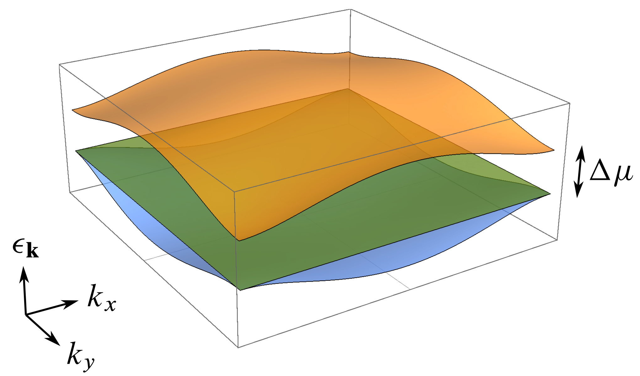
Figure 3.5: Doublon energy bands for the Lieb lattice. The effective local potential opens a gap between the upper band and the rest. The driving allows the band width to be reduced, flattening the bands, while keeping the gap the same.

When studying quantum walks [99], i.e., the coherent evolution of particles in networks, it is natural to ask about the probability of finding a particle that was initially on site $i$ to be on site $j$ after a certain time $t$, that is, $p_{ij}(t)\equiv\lvert\langle i\rvert U(t)\lvert j\rangle\rvert^{2}=\lvert\langle i\rvert e^{-iHt}\lvert j\rangle\rvert^{2}$. Using (3.23) as the effective single-particle Hamiltonian for the doublon, we define $p_{A}(t)\equiv\sum_{i,\,j\in A}p_{ij}(t)/N_{A}$, which is the probability for the doublon to remain in sublattice $A$ at time $t$; $N_{A}$ is the total number of sites that belong to sublattice $A$. To demonstrate sublattice confinement, we can compute the long-time average

$$\mkern 1.5mu\overline{\mkern-1.5mup_{A}\mkern-1.5mu}\mkern 1.5mu\equiv\lim_{t\to\infty}\frac{1}{t}\int_{0}^{t}d\mkern-1.5mu{t^{\prime}}\,p_{A}(t^{\prime})\,.$$ (3.29)

According to the definition, the probability $p_{A}(t)$ is $\lVert U_{A}(t)\rVert^{2}/N_{A}$, where $\lVert\cdot\rVert$ denotes the Hilbert-Schmidt norm, and $U_{A}(t)=P_{A}U(t)P_{A}$ is the time evolution operator projected on the subspace of the $A$ sublattice. Using the spectral decomposition

$$U(t)=\mathop{{\sum}}_{\mathbf{k}}\mathop{{\sum}}_{\alpha=0,\pm}e^{-i\epsilon^{\alpha}_{\mathbf{k}}t}\left\lvert u^{\alpha}_{\mathbf{k}}\right\rangle\left\langle u^{\alpha}_{\mathbf{k}}\right\rvert\,,$$ (3.30)

we can express

$$\lVert U_{A}(t)\rVert^{2} =\mathop{{\sum}}_{\mathbf{k}}\left\lvert\frac{e^{-i\epsilon^{+}_{\mathbf{k}}t}}{1+g_{+}(\mathbf{k})}+\frac{e^{-i\epsilon^{-}_{\mathbf{k}}t}}{1+g_{-}(\mathbf{k})}\right\rvert^{2}$$ (3.31)

$$=\mathop{{\sum}}_{\mathbf{k},\,\alpha=\pm}\frac{1}{\left[1+g_{\alpha}(\mathbf{k})\right]^{2}}+\mathop{{\sum}}_{\mathbf{k}}\frac{2\cos\left(\epsilon^{+}_{\mathbf{k}}t-\epsilon^{-}_{\mathbf{k}}t\right)}{\left[1+g_{+}(\mathbf{k})\right]\left[1+g_{-}(\mathbf{k})\right]}\,,$$ (3.32)

where we have defined $g_{\pm}(\mathbf{k})=\left[\lvert f_{1}(\mathbf{k})\rvert^{2}+\lvert f_{2}(\mathbf{k})\rvert^{2}\right]\left(\epsilon^{\pm}_{\mathbf{k}}\right)^{-2}$. The time average is, thus, given by

$$\mkern 1.5mu\overline{\mkern-1.5mup_{A}\mkern-1.5mu}\mkern 1.5mu=\frac{1}{V}\int_{\mathrm{FBZ}}d^{2}\mathbf{k}\,\left\{\frac{1}{\left[1+g_{+}(\mathbf{k})\right]^{2}}+\frac{1}{\left[1+g_{-}(\mathbf{k})\right]^{2}}\right\}\,.$$ (3.33)

Here, we have taken the thermodynamic limit, replacing the sum over momenta by an integral on the first Brillouin zone (FBZ); $V$ stands for the FBZ area. As can be seen in Fig. 3.6(a) the probability $\mkern 1.5mu\overline{\mkern-1.5mup_{A}\mkern-1.5mu}\mkern 1.5mu$ can be enhanced by tuning the ratio $\Delta\mu/J_{\mathrm{eff}}$ to larger values, meaning that it is possible to confine the doublon’s dynamics to a single sublattice by suitably changing the ac field parameters. We have also computed the dependence of $\mkern 1.5mu\overline{\mkern-1.5mup_{A}\mkern-1.5mu}\mkern 1.5mu$ with the magnetic flux threading the smallest plaquette (the smallest closed path in the lattice), see Fig. 3.6(b); however, its variation turns out to be minor with $\mkern 1.5mu\overline{\mkern-1.5mup_{A}\mkern-1.5mu}\mkern 1.5mu$ gently increasing as the flux is tuned away from $2\Phi/\Phi_{0}=1/2$. A much stronger dependence is observed for the $\mathcal{T}_{3}$ than for the Lieb lattice. This is to be expected as Aharonov-Bohm phases have more dramatic effects in the $\mathcal{T}_{3}$ lattice, notably the caging effect that occurs for a magnetic flux $\Phi/\Phi_{0}=1/2$ in the singly-charged particle case [100].

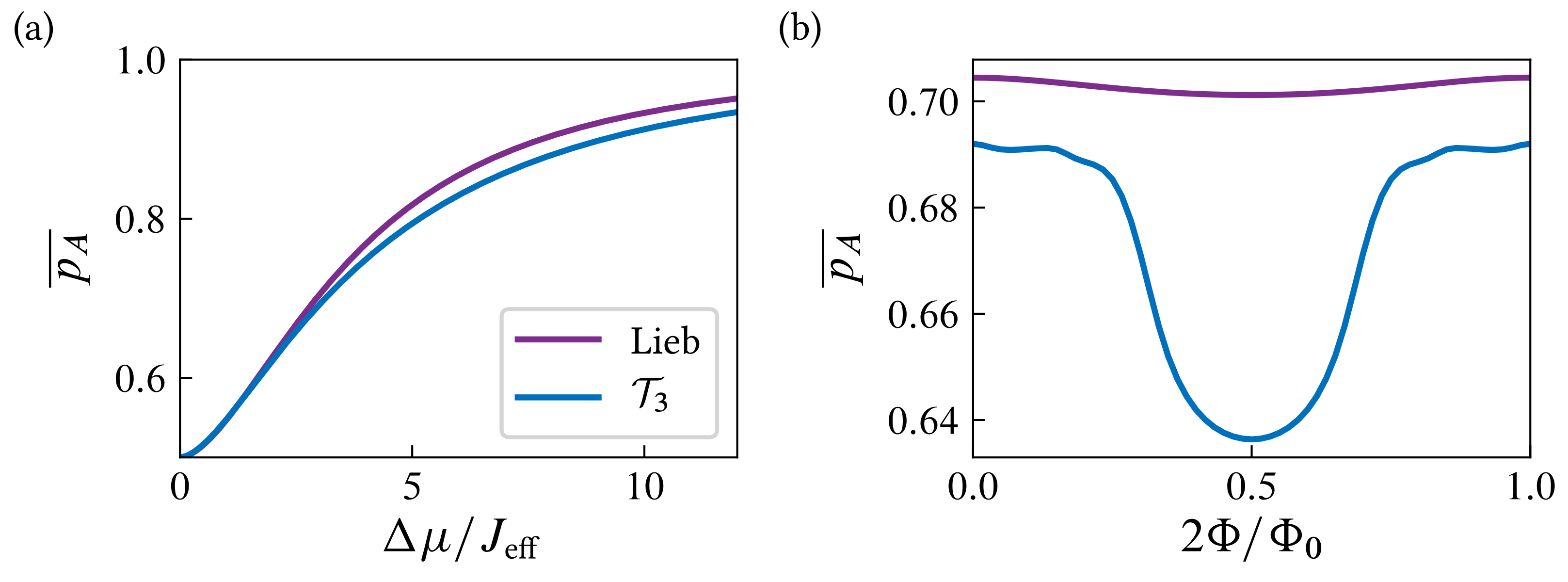
Figure 3.6: Probability to remain in sublattice $A$ as a function of the ratio $\Delta\mu/J_{\mathrm{eff}}$, for $\Phi=0$ (a), and as a function of the magnetic flux per plaquette, for $\Delta\mu/J_{\mathrm{eff}}=3$ (b).

It is worth mentioning that a similar effect constrains the motion of doublons in any lattice with boundaries. The sites on the edges necessarily have fewer neighbors than those in the bulk and therefore have a smaller chemical potential. This produces eigenstates localized on the edges, which are of the Shockley or Tamm type. As a consequence, the doublon’s dynamics can be confined to just the edges of the lattice. Furthermore, since having non-trivial topology in 2D does not require any symmetry, in the presence of a nonzero magnetic flux any lattice can support both Shockley-like edge states and topological chiral edge states at the same time. Let us be more specific. When comparing the effective model (3.23) with that of a Chern insulator [7], the only difference is the local chemical potential term. It is well known that strong disorder potentials eventually destroy the topological properties of Chern insulators as they transition to a trivial Anderson insulator by a mechanism known as “levitation and annihilation” of extended states [101, 102]. Nonetheless, the chemical potential term in our Hamiltonian constitutes a very particular form of disorder that does not affect the topology of the system. In Fig. 3.7 we show the energy spectrum of a ribbon of the Lieb lattice in the presence of a magnetic flux. There, we can observe topological edge states appearing in the minigaps opened by the magnetic flux that propagate in a fixed direction depending on their energy and the edge where they localize. We can also find Shockley-like edge states that can propagate in both directions along each edge. When reducing the effective hopping, these states are pulled further out of the bulk minibands, making them interfere less with the topological edge states. After this analysis we conclude that, depending on their energy, a doublon can propagate chirally or not along the edges of a lattice threaded by a magnetic flux.

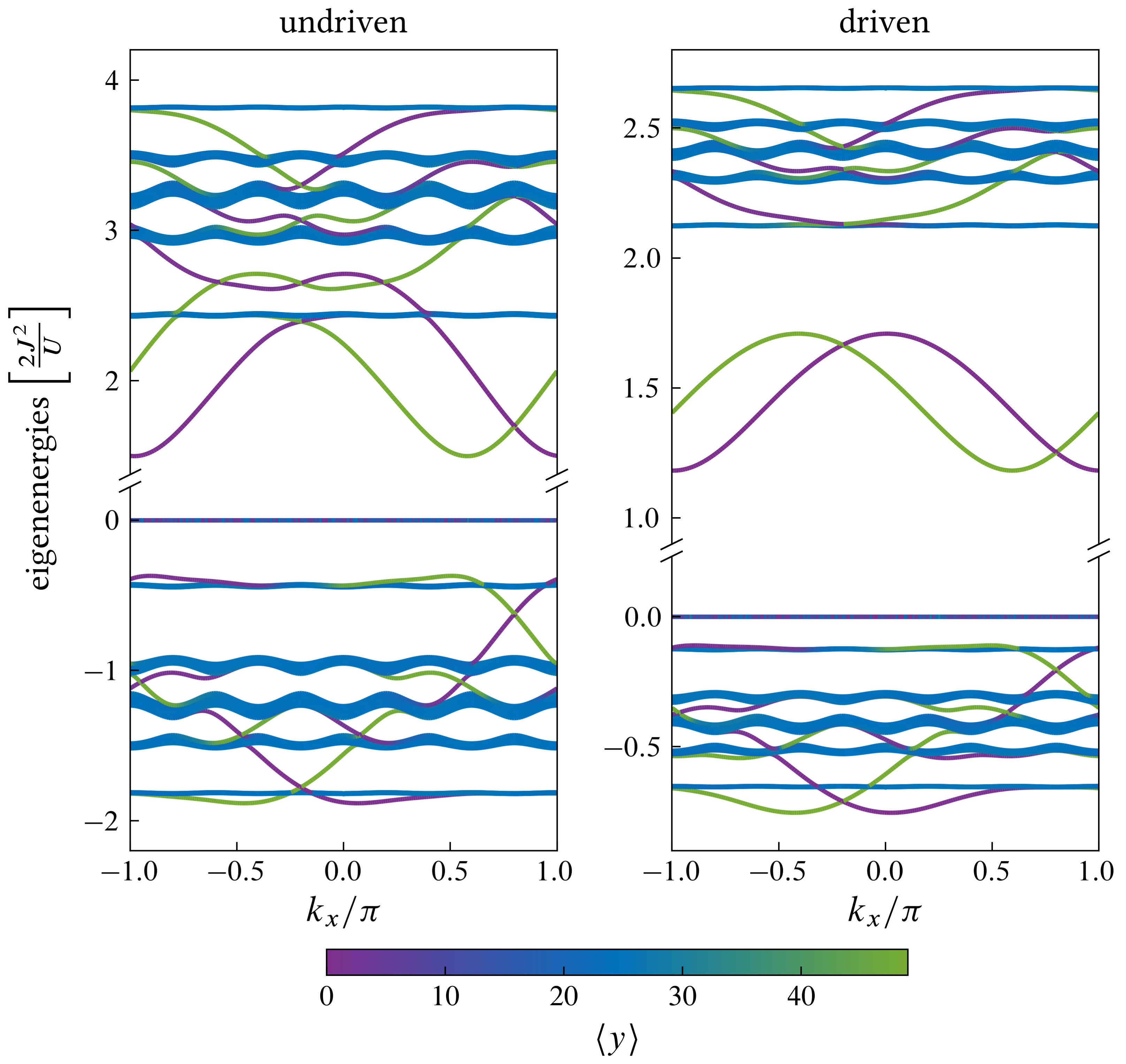
Figure 3.7: Energy spectrum of a finite ribbon of the Lieb lattice, with $N_{y}=50$ unit cells along the $y$ direction in the presence of a magnetic flux $\Phi/\Phi_{0}=1/10$. The ac field in the case shown in the right plot is such that $\mathcal{J}_{0}\left(2Ea/\omega\right)=1/2$. The color indicates the localization of the state along the finite dimension of the lattice: green and purple denote states localized on each edge of the ribbon (topological and Shockley-like edge states), while blue is used for bulk states that are not localized (minibands). Topological edge states always connect different minibands, while Shockley edge states do not necessarily do so.

3.3.  Doublon decay in dissipative systems

The high controllability and isolation achieved in cold atom experiments make them a great platform for observing doublons. But can doublons be observed in other kind of systems? Nowadays, solid-state devices such as quantum dot arrays are being investigated as platforms for quantum simulation. However, phonons, nuclear spins, and fluctuating charges and currents make for a much noisier environment in these setups as compared with others [71]. In this section we investigate how the coupling to the environment may affect the stability of doublons in QD arrays and give an estimate of their lifetime in current devices.

We will analyze the case of a 1D array of $N$ quantum dots, see Fig. 3.8. Electrons trapped in the QD array are modelled by the Hubbard Hamiltonian with an homogeneous hopping amplitude $J$ and interaction strength $U$. For the environment, we assume the chain is coupled to several independent baths of harmonic oscillators. The system and the environment can be modelled as a whole by the Hamiltonian $H=H_{S}+H_{B}+H_{I}$, with

$$H_{S} =-J\mathop{{\sum}}_{j,\,\sigma}\left(c^{\dagger}_{j+1\sigma}c_{j\sigma}+\mathrm{H.c.}\right)+U\mathop{{\sum}}_{j}n_{j{\uparrow}}n_{j{\downarrow}}\,,$$ (3.34)

$$H_{B} =\mathop{{\sum}}_{j,\,n}\omega_{n}a^{\dagger}_{nj}a_{nj}\,,$$ (3.35)

$$H_{I} =\mathop{{\sum}}_{j}X_{j}B_{j}\,,\quad B_{j}=\mathop{{\sum}}_{n}g_{n}(a^{\dagger}_{nj}+a_{nj})\,.$$ (3.36)

Here, $B_{j}$ is the collective coordinate of the $j$th bath that couples to the system operator $X_{j}$, which will be specified below. Moreover, we assume that all baths are equal and statistically independent.

Figure 3.8: Schematic picture of the system under consideration. A QD array modelled as a tight-binding 1D lattice is occupied by two electrons. An initial state with a doubly occupied site (doublon) may decay dissipatively into a single-occupancy state with lower energy. The released energy is of the order of the on-site interaction $U$ and will be absorbed by the heat baths representing environmental charge and current noise.

In the Markovian regime, the time evolution of the system’s density matrix $\rho$, can be suitably described by a Bloch-Redfield master equation of the form [67, 66] (see appendix 3.B)

$$\dot{\rho} =-i[H_{S},\rho]-\mathop{{\sum}}_{j}[X_{j},[Q_{j},\rho]]-\mathop{{\sum}}_{j}[X_{j},\{R_{j},\rho\}]$$

$$\equiv-i[H_{S},\rho]+\mathcal{L}[\rho]\,,$$ (3.37)

with the anticommutator $\{A,B\}=AB+BA$ and

$$Q_{j} =\frac{1}{\pi}\int_{0}^{\infty}d\mkern-1.5mu{\tau}\,\int_{0}^{\infty}d\mkern-1.5mu{\omega}\,\mathcal{S}(\omega)\tilde{X}_{j}(-\tau)\cos\omega\tau\,,$$ (3.38)

$$R_{j} =\frac{-i}{\pi}\int_{0}^{\infty}d\mkern-1.5mu{\tau}\,\int_{0}^{\infty}d\mkern-1.5mu{\omega}\,\mathcal{J}(\omega)\tilde{X}_{j}(-\tau)\sin\omega\tau\,.$$ (3.39)

The tilde denotes the interaction picture, $\tilde{X}_{j}(-\tau)={e^{-iH_{S}\tau}X_{j}e^{iH_{S}\tau}}$, while the spectral density of the baths is $\mathcal{J}(\omega)=\pi\sum_{n}|g_{n}|^{2}\delta(\omega-\omega_{n})$, and ${\mathcal{S}(\omega)=\mathcal{J}(\omega)\coth(\beta\omega/2)}$ is the Fourier transformed of the symmetrically ordered equilibrium autocorrelation function $\langle\{B_{j}(\tau),B_{j}(0)\}\rangle/2$. $\mathcal{J}(\omega)$ and $\mathcal{S}(\omega)$ are independent of the bath subindex $j$ since all baths are identical. We will assume an ohmic spectral density ${\mathcal{J}(\omega)=\pi\alpha\omega/2}$, where the dimensionless parameter $\alpha$ characterizes the dissipation strength.

3.3.1.  Charge noise

Fluctuations of the background charges in the substrate essentially act upon the charge distribution of the chain. We model it by coupling the occupation of each site to a heat bath, such that

$$H_{I}=\mathop{{\sum}}_{j,\,\sigma}n_{j\sigma}B_{j}\,,\quad X_{j}=n_{j{\uparrow}}+n_{j{\downarrow}}\,.$$ (3.40)

This fully specifies the master equation (3.37).

To get a qualitative understanding of the decay dynamics of a doublon, let us start by discussing the time evolution of the total double occupancy

$$D\equiv\mathop{{\sum}}_{j}n_{j{\uparrow}}n_{j{\downarrow}}=\mathop{{\sum}}_{j}d^{\dagger}_{j}d_{j}\,,$$ (3.41)

for an initial doublon state, shown in Fig. 3.9(a). For $\alpha=0$, i.e., in the absence of dissipation, the two electrons will essentially remain together throughout time evolution. However, since the doublon states are not eigenstates of the system Hamiltonian, we observe some slight oscillations of the double occupancy. Still the time average of this quantity stays close to unity. On the contrary, if the system is coupled to a bath, doublons will be able to split, releasing energy into the environment. Then the density operator eventually becomes the thermal state $\rho_{\infty}\propto e^{-\beta H_{S}}$. Depending on the temperature and the interaction strength, the corresponding asymptotic doublon occupancy $\langle D\rangle_{\infty}$ may still assume an appreciable value.

To gain a quantitative insight, we decompose our master equation (3.37) into the system eigenbasis and obtain a form convenient for numerical treatment (appendix 3.B). A typical time evolution of the total double occupancy exhibits an almost monoexponential decay, such that the doublon life time $T_{1}$ can be defined as the time when

$$\frac{\langle D\rangle_{T_{1}}-\langle D\rangle_{\infty}}{1-\langle D\rangle_{\infty}}=\frac{1}{e}\,.$$ (3.42)

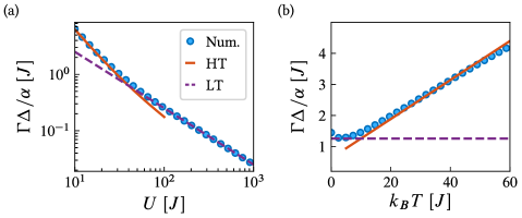
Figure 3.10: Comparison between the numerically computed decay rate and the analytic formulas (3.50) and (3.51) for a chain with $N=5$ sites and periodic boundary conditions in the case of charge noise. The dissipation strength is $\alpha=0.02$. (a) Dependence on the interaction strength for a fixed temperature $k_{B}T=20J$. (b) Dependence on the temperature for a fixed interaction strength $U=20J$.

The corresponding decay rate $\Gamma=1/T_{1}$ is shown in Fig. 3.10 as a function of the temperature and interaction strength for a fixed small $\alpha$.

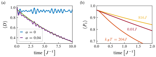
Figure 3.9: Time evolution of the double occupancy in a system with charge noise. The initial state consists of a doublon localized in a particular site of a chain with periodic boundary conditions. Parameters: $N=5$, $U=10J$ and $\alpha=0.04$. (a) Comparison between free dynamics ($\alpha=0$) and dissipative dynamics ($\alpha\neq 0$). Temperature is set to $k_{B}T=0.01J$. The green line corresponds to the occupancy of the high-energy subspace for the case with $\alpha\neq 0$ and illustrates the bound given in Eq. (3.44). (b) Decay of the high-energy subspace occupancy for different temperatures ranging from $0.01J$ to $1000J$. The slope of the curves at time $t=0$ is the same in all cases and coincides with the value given by Eq. (3.47).

An analytical estimate for the decay rates can often be gained from the behavior at the initial time $t=0$, i.e. from $\dot{\rho}_{0}$. In the present case, however, the calculation is hindered by the fast initial oscillations witnessed in Fig. 3.9(a). To circumvent this problem, we focus instead on the occupancy of the high-energy subspace, $\langle P_{1}\rangle$, with $P_{1}$ being the projector onto the high energy subspace, shown in Fig. 3.9(b). Using the Schrieffer-Wolff transformation derived in section 3.1 we can express it in terms of the projector onto the doublon subspace, $P_{D}$, as

$$P_{1}=P_{D}+\frac{1}{U}\left(H^{+}_{J}+H^{-}_{J}\right)+O\left(U^{-2}\right)\,.$$ (3.43)

It turns out that this quantity evolves more smoothly while it decays also on the time scale $T_{1}$. To understand this similarity, notice that

$$\left\lvert\operatorname{tr}\left(P_{1}\rho\right)-\operatorname{tr}\left(D\rho\right)\right\rvert\leq\sqrt{2}\lVert\rho\rVert\sqrt{N-\operatorname{tr}\left(P_{1}P_{D}\right)}\simeq\frac{2\sqrt{2N}J}{U}\,,$$ (3.44)

where we have used the Cauchy-Schwarz inequality for the inner product of operators, $(A,B)=\operatorname{tr}\left(A^{\dagger}B\right)$, and the perturbative expansion of $P_{1}$ mentioned before. The reason for its lack of fast oscillations is that the projector $P_{1}$ commutes with the system Hamiltonian, so that its expectation value is determined solely by dissipation.

Following our hypothesis of a monoexponential decay, we expect

$$\langle P_{1}\rangle\simeq{\Delta e^{-\Gamma t}+\langle P_{1}\rangle_{\infty}}\,,$$ (3.45)

therefore

$$\Gamma\simeq-\frac{1}{\Delta}\left.\frac{d\langle P_{1}\rangle}{dt}\right|_{t=0}=-\frac{\operatorname{tr}\left(P_{1}\mathcal{L}[\rho_{0}]\right)}{\langle P_{1}\rangle_{0}-\langle P_{1}\rangle_{\infty}}\,.$$ (3.46)

This expression still depends slightly on the specific choice of the initial doublon state. To obtain a more global picture, we consider an average over all doublon states, which can be performed analytically [103] (see appendix 3.C). Substituting the expression for the Liouvillian in Eq. (3.46), we find the average decay rate

$$\mkern 1.5mu\overline{\mkern-1.5mu\Gamma\mkern-1.5mu}\mkern 1.5mu=\frac{1}{N\Delta}\mathop{{\sum}}_{j}\operatorname{tr}\left(P_{D}[Q_{j},[X_{j},P_{1}]]\right)-\operatorname{tr}\left(P_{D}\{R_{j},[X_{j},P_{1}]\}\right)\,.$$ (3.47)

For a further simplification, we have to evaluate the expressions (3.38) and (3.39) which is possible by approximating the interaction picture coupling operator as $\tilde{X}_{j}(-\tau)\simeq X_{j}-i\tau[H_{S},X_{j}]$. This is justified as long as the decay of the environmental excitations is much faster than the typical system evolution, i.e., in the high-temperature regime (HT). Inserting our approximation for $\tilde{X}_{j}$ and neglecting the imaginary part of the integrals, we arrive at

$$Q_{j}\simeq\frac{1}{2}\lim_{\omega\rightarrow 0^{+}}\mathcal{S}(\omega)X_{j}=\frac{\pi}{2}\alpha k_{B}TX_{j}\,,$$ (3.48)

$$R_{j}\simeq-\frac{1}{2}\lim_{\omega\rightarrow 0^{+}}\mathcal{J}^{\prime}(\omega)[H_{S},X_{j}]=\frac{\pi}{4}\alpha[H_{S},X_{j}]\,.$$ (3.49)

With these expressions, Eq. (3.47) results in a temperature independent decay rate. Notice that any temperature dependence stems from the $Q_{j}$ in the first term of Eq. (3.47), which vanishes in the present case. While this observation agrees with the numerical findings in Fig. 3.9(b) for very short times, it does not reflect the temperature dependent decay of $\langle P_{1}\rangle$ at the more relevant intermediate stage.

This particular behavior hints at the mechanism of the bath-induced doublon decay. Let us remark that for the coupling to charge noise, $X_{j}$ commutes with $D$. Therefore, the initial state is robust against the influence of the bath. Only after mixing with the single-occupancy states due to the coherent dynamics, the system is no longer in an eigenstate of $X_{j}$, such that decoherence and dissipation become active. Thus, it is the combined action of the system’s unitary evolution and the effect of the environment which leads to the doublon decay. An improved estimate of the decay rate, can be calculated by averaging the transition rate of states from the high-energy subspace to the low-energy subspace. Let us first focus on regime $k_{B}T\gtrsim U$ in which we can evaluate the operators $Q_{j}$ in the high-temperature limit. Then the average rate can be computed using expression (3.47) replacing $P_{D}$ by $P_{1}$. With the perturbative expansion of $P_{1}$ in Eq. (3.43) we obtain to leading order in $J/U$ the averaged rate

$$\mkern 1.5mu\overline{\mkern-1.5mu\Gamma\mkern-1.5mu}\mkern 1.5mu_{\mathrm{HT}}\simeq\frac{4\pi\alpha J^{2}}{U^{2}\Delta}\left(2k_{B}T+U\right)\,,$$ (3.50)

valid for periodic boundary conditions. For open boundary conditions, the rate acquires an additional factor $(N-1)/N$. Notice that we have neglected back transitions via thermal excitations from singly occupied states to doublon states. We will see that this leads to some deviations when the temperature becomes extremely large. Nevertheless, we refer to this case as the high-temperature limit.

In the opposite limit, for temperatures ${k_{B}T<U}$, the decay rate saturates at a constant value. To evaluate $\mkern 1.5mu\overline{\mkern-1.5mu\Gamma\mkern-1.5mu}\mkern 1.5mu$ in this limit, it would be necessary to find an expression for $\tilde{X}_{j}(-\tau)$ dealing properly with the $\tau$-dependence for evaluating the noise kernel, a formidable task that may lead to rather involved expressions. However, one can make some progress by considering the transition of one initial doublon to one particular single-occupancy state. This corresponds to approximating our two-particle lattice model by a dissipative two-level system for which the decay rates in the Ohmic case can be taken from the literature [104, 105] (see appendix 3.D). Relating $J$ to the tunnel matrix element of the two-level system and $U$ to the detuning, we obtain the temperature-independent expression

$$\mkern 1.5mu\overline{\mkern-1.5mu\Gamma\mkern-1.5mu}\mkern 1.5mu_{\text{LT}}\simeq\frac{8\pi\alpha J^{2}}{U\Delta}\,,$$ (3.51)

which formally corresponds to Eq. (3.50) with the temperature set to $k_{B}T=U/2$.

3.3.2.  Current noise

Fluctuating background currents mainly couple to the tunnel matrix elements of the system. Then the system-bath interaction is given by

$$H_{I}=\mathop{{\sum}}_{j,\,\sigma}\left(c^{\dagger}_{j+1\sigma}c_{j\sigma}+c^{\dagger}_{j\sigma}c_{j+1\sigma}\right)B_{j}\,,$$ (3.52)

$$X_{j}=c^{\dagger}_{j+1\sigma}c_{j\sigma}+c^{\dagger}_{j\sigma}c_{j+1\sigma}\,.$$ (3.53)

Depending on the boundary conditions, the sum may include the term connecting the first and last QD of the array. The main difference with respect to the case of charge noise is that now $H_{I}$ does not commute with the projector onto the doublon subspace and, thus, generally ${\operatorname{tr}\left(D\mathcal{L}[\rho_{0}]\right)\neq 0}$. This allows doublons to decay without having to mix with single-occupancy states. Therefore, for the same value of the dissipation strength $\alpha$, the decay may be much faster.

As in the last section, we proceed by calculating analytical estimates for the decay rates. However, the time evolution is no longer monoexponential. In this case, we estimate the rate from the slope of the occupancy $\langle P_{1}\rangle$ at initial time,

$$\Gamma\simeq-\left.\frac{d\langle P_{1}\rangle}{dt}\right|_{t=0}=-\operatorname{tr}\left(P_{1}\mathcal{L}[\rho_{0}]\right)\ .$$ (3.54)

We again perform the average over all doublon states for $\rho_{0}$ in the limits of high and low temperatures. For periodic boundary conditions, we obtain to lowest order in $J/U$ the high and low temperature rates

$$\mkern 1.5mu\overline{\mkern-1.5mu\Gamma\mkern-1.5mu}\mkern 1.5mu_{\mathrm{HT}} =2\pi\alpha\left(2k_{B}T+U\right)\,,$$ (3.55)

$$\mkern 1.5mu\overline{\mkern-1.5mu\Gamma\mkern-1.5mu}\mkern 1.5mu_{\text{LT}} =4\pi\alpha U\,,$$ (3.56)

respectively, while open boundary conditions lead to the same expressions but with a correction factor $(N-1)/N$. In Fig. 3.11, we compare these results with the numerically evaluated ones as a function of the interaction and the temperature. Both show that the analytical approach correctly predicts the (almost) linear behavior at large values of $U$ and $k_{B}T$, as well as the saturation for small values. However, the approximation slightly overestimates the influence of the bath.

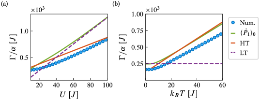
Figure 3.11: Numerically obtained decay rate in comparison with the approximations (3.54), (3.55) and (3.56) for a chain with $N=5$ sites and periodic boundary conditions in the case of current noise with strength $\alpha=0.02$. The results are plotted as a function of (a) the interaction and the temperature $k_{B}T=20J$ and (b) for a fixed interaction $U=20J$ as a function of the temperature.

While the rates reflect the decay at short times, it is worthwhile to comment on the long time behavior under the influence of current noise. As it turns out, the steady state is not unique. The reason for this is the existence of a doublon state ${\lvert\Phi\rangle=\frac{1}{\sqrt{N}}\sum_{j=1}^{N}(-1)^{j}c^{\dagger}_{j{\uparrow}}c^{\dagger}_{j{\downarrow}}\lvert 0\rangle}$ which is an eigenstate of $H_{S}$ without any admixture of single-occupancy states. Since $X_{j}\lvert\Phi\rangle=0$ for all $j$, current noise may affect the phase of ${\lvert\Phi\rangle}$, but cannot induce its dissipative decay. For a closed chain with an odd number of sites, by contrast, the alternating phase of the coefficients of $\lvert\Phi\rangle$ is incompatible with periodic boundary conditions, unless a flux threads the ring. As a consequence, the state of the chain eventually becomes the thermal state $\rho_{\infty}\propto e^{-\beta H_{S}}$. The difference is manifest in the final value of the doublon occupancy at low temperatures. For closed chains with an odd number of sites, it will fully decay, while in the other cases, the population of $\lvert\Phi\rangle$ will survive.

3.3.3.  Experimental implications

A current experimental trend is the fabrication of larger QD arrays [106, 39], which triggered our question on the feasibility of doublon experiments in solid-state systems. While the size of these arrays would be sufficient for this purpose, their dissipative parameters are not yet fully known. For an estimate we therefore consider the values for GaAs/InGaAs quantum dots which have been determined recently via Landau-Zener interference [71]. Notice, that for the strength of the current noise, only an upper bound has been reported. We nevertheless use this value, but keep in mind that it leads to a conservative estimate. In contrast to the former sections, we now compute the decay for the simultaneous action of charge noise and current noise.

Figure 3.12 shows the $T_{1}$ times for two different interaction strengths. It reveals that for low temperatures $T\lesssim J/k_{B}T$, the life time is essentially constant, while for larger temperatures, it decreases moderately until $k_{B}T$ comes close to the interaction $U$. For higher temperatures, $\Gamma$ starts to grow linearly. On a quantitative level, we expect life times of the order $T_{1}\sim 5$ ns already for moderately low temperatures $T\lesssim 100$ mK. Since we employed the value of the upper bound for the current noise, the life time might be even larger.

Considering the estimates for the decay rates at low temperatures, Eqs. (3.51) and (3.56), separately, we conclude that for smaller values of $U$, current noise becomes less important, while the impact of charge noise grows. Therefore, a strategy for reaching larger $T_{1}$ times is to design QD arrays with smaller on-site interaction, such that the ratio $U/J$ becomes more favorable. The largest $T_{1}$ is expected in the case in which both low-temperature decay rates are equal, $\mkern 1.5mu\overline{\mkern-1.5mu\Gamma\mkern-1.5mu}\mkern 1.5mu_{\mathrm{LT}}^{\mathrm{charge}}=\mkern 1.5mu\overline{\mkern-1.5mu\Gamma\mkern-1.5mu}\mkern 1.5mu_{\mathrm{LT}}^{\mathrm{current}}$, which for the present experimental parameters is found at $U\sim 10J$. This implies that in an optimized device, the doublon life times could be larger by one order of magnitude to reach values of $T_{1}\sim 50$ ns, which is corroborated by the data in the inset of Fig. 3.12.

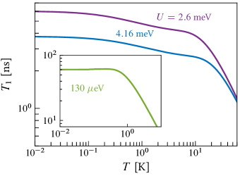
Figure 3.12: Doublon life time as a function of the temperature for different interaction strengths. The parameters are: $\alpha_{\mathrm{charge}}=3\times 10^{-4}$, $\alpha_{\mathrm{current}}=5\times 10^{-6}$, and $J=13\,\mu$eV. The $T_{1}$ time has been measured for a doublon starting in the middle of a chain with $N=5$ and open boundary conditions. Inset: $T_{1}$ time for the optimized value of the interaction, $U=10J=130\,\mu$eV and a current noise with $\alpha_{\mathrm{current}}=2\times 10^{-6}$.

3.4.  Summary

For understanding the dynamics of doublons, we have derived an effective single-particle Hamiltonian taking into account also the effect of a periodic driving on the lattice. It contains two terms: one corresponding to an effective doublon hopping renormalized by the driving, and another one corresponding to an effective on-site chemical potential, with the peculiarity of being proportional to the number of neighbors of each site. Importantly, in the regime where the Hubbard interaction is larger than the frequency of the driving and these are both larger than any other energy scale of the system, the driving allows to tune the doublon hopping independently of the effective chemical potential. This produces several interesting phenomena regarding the doublons’ motion:

1. In any finite lattice doublons experience an effective chemical potential difference between the sites on the edges and the rest of the sites. This allows the generation of Shockley-like edge states by reducing the doublon hopping with the driving.

2. In the SSH-Hubbard model, the chemical potential difference between the ending sites of the chain and the rest of the sites causes the disappearance of the topological edge states for doublons. This chemical potential difference breaks the chiral symmetry of the SSH model, which is essential for having non-trivial topology. On the other hand, for 2D lattices threaded by a magnetic flux, no symmetry is required for having non-trivial topology, thus, they do support topological edge states for doublons, which may coexist with Shockley-like edge states induced by the driving.

3. Both topological and Shockley-like edge states allow for the direct long-range transfer of doublons between distant sites in the edges of a finite lattice.

4. In lattices with sites with different coordination numbers it is possible to confine the doublon’s motion to a single sublattice at the expense of slowing it down by reducing the doublon hopping with the driving.

We have also studied the stability of doublons in quantum dot arrays in the presence of charge noise and current noise. While the dependence on temperature of the doublon’s lifetime $T_{1}$ is similar for both types of noise, the dependence with the interaction strength $U$ is very different. For charge noise $T_{1}\sim U$, whereas for current noise $T_{1}\sim U^{-1}$, in the low temperature regime ($k_{B}T<U$). In current devices we predict a doublon lifetime of the order of 10 ns, although it can be improved up to one order of magnitude in devices specifically designed to that end.

Appendices

Appendix 3.A Effective Hamiltonian for doublons

We start from a Fermi-Hubbard model with an ac field that couples to the particle density and a magnetic flux that introduces complex phases in the hoppings. The Hamiltonian of the system is $H(t)=H_{J}+H_{U}+H_{AC}(t)$, with

$$H_{AC}(t)=\mathop{{\sum}}_{j}V_{j}(t)(n_{j,{\uparrow}}+n_{j,{\downarrow}})\,.$$ (3.57)

For a time-periodic Hamiltonian, $H(t+T)=H(t)$, with $T=2\pi/\omega$, Floquet’s theorem allows us to write the time-evolution operator as

$$U(t_{2},t_{1})=e^{-iK(t_{2})}e^{-iH_{\mathrm{eff}}(t_{2}-t_{1})}e^{iK(t_{1})}\,,$$ (3.58)

where $H_{\mathrm{eff}}$ is a time-independent, effective Hamiltonian, and $K(t)$ is a $T$-periodic Hermitian operator. $H_{\mathrm{eff}}$ governs the long-term dynamics, whereas $e^{-iK(t)}$, also known as the micromotion-operator, accounts for the fast dynamics occurring within a period. Following several perturbative methods [62, 63], it is possible to find expressions for these operators as power series in $1/\omega$,

$$H_{\mathrm{eff}}=\mathop{{\sum}}\limits_{n=0}^{\infty}\frac{H_{\mathrm{eff}}^{(n)}}{\omega^{n}}\,,\quad K(t)=\mathop{{\sum}}\limits_{n=0}^{\infty}\frac{K^{(n)}(t)}{\omega^{n}}\,.$$ (3.59)

These are known in the literature as high-frequency expansions (HFE). The different terms in these expansions have a progressively more complicated dependence on the Fourier components of the original Hamiltonian,

$$H_{q}=\frac{1}{T}\int_{0}^{T}d\mkern-1.5mu{t}\,H(t)e^{i\omega qt}\,.$$ (3.60)

The first three of them are:

$$H_{\mathrm{eff}}^{(0)} =H_{0}\,,$$ (3.61)

$$H_{\mathrm{eff}}^{(1)} =\mathop{{\sum}}\limits_{q\neq 0}\frac{H_{-q}H_{q}}{q}\,,$$ (3.62)

$$H_{\mathrm{eff}}^{(2)} =\mathop{{\sum}}\limits_{q,\,p\neq 0}\left(\frac{H_{-q}H_{q-p}H_{p}}{qp}-\frac{H_{-q}H_{q}H_{0}}{q^{2}}\right)\,.$$ (3.63)

Before deriving the effective Hamiltonian, it is convenient to transform the original Hamiltonian into the rotating frame with respect to both the interaction and the ac field [107],

$$\tilde{H}(t)=\mathcal{U}^{\dagger}(t)H(t)\mathcal{U}(t)-i\mathcal{U}^{\dagger}(t)\partial_{t}\mathcal{U}(t)\,,$$ (3.64)

$$\mathcal{U}(t)=\exp\left[-iH_{U}t-i\int d\mkern-1.5mu{t}\,H_{AC}(t)\right]\,.$$ (3.65)

Noting that for fermions

$$e^{iH_{U}t}c^{\dagger}_{i\sigma}c_{j\sigma}e^{-iH_{U}t}=\left[1-n_{i\bar{\sigma}}\left(1-e^{iUt}\right)\right]c^{\dagger}_{i\sigma}c_{j\sigma}\left[1-n_{j\bar{\sigma}}\left(1-e^{-iUt}\right)\right]\,,$$ (3.66)

the Hamiltonian in the rotating frame can be written as

$$\tilde{H}(t) =-\mathop{{\sum}}_{i,\,j,\,\sigma}J_{ij}(t)\left(T^{0}_{ij\sigma}+e^{iUt}T^{+}_{ij\sigma}+e^{-iUt}T^{-}_{ij\sigma}\right)\,,$$ (3.67)

with $J_{ij}(t)=J_{ij}e^{i\mathbf{A}(t)\cdot\mathbf{d}_{ij}}$. Note that this is a different way of expressing the coupling to an electric field described by the vector potential $\mathbf{A}(t)$. In the case of circular polarization, $\mathbf{A}(t)=\left(\sin(\omega t),-\cos(\omega t)\right)E/\omega$; $\mathbf{d}_{ij}=\mathbf{r}_{i}-\mathbf{r}_{j}$ is the vector connecting sites $i$ and $j$. We have defined:

$$T^{0}_{ij\sigma}=n_{i\bar{\sigma}}c^{\dagger}_{i\sigma}c_{j\sigma}n_{j\bar{\sigma}}+h_{i\bar{\sigma}}c^{\dagger}_{i\sigma}c_{j\sigma}h_{j\bar{\sigma}}\,,$$ (3.68)

$$T^{+}_{ij\sigma}=n_{i\bar{\sigma}}c^{\dagger}_{i\sigma}c_{j\sigma}h_{j\bar{\sigma}}\,,\quad T^{-}_{ij\sigma}=(T^{+}_{ji\sigma})^{\dagger}=h_{i\bar{\sigma}}c^{\dagger}_{i\sigma}c_{j\sigma}n_{j\bar{\sigma}}\,.$$ (3.69)

The operators $T^{0}_{ij\sigma}$ involve hopping processes that conserve the total double occupancy, while $T^{+}_{ij\sigma}$ and $T^{-}_{ij\sigma}$ raise and lower the total double occupancy respectively.

In order to apply the HFE method we need to find a common frequency. We will consider first the resonant regime, $U=l\omega$, and then, by means of analytical continuation, obtain the strongly-interacting limit ($U\gg\omega>J$) and the ultrahigh-frequency limit ($\omega\gg U>J$). The Fourier components of $\tilde{H}(t)$ are

$$\tilde{H}_{q}=-\mathop{{\sum}}_{i,\,j,\,\sigma}\left(J_{ij,q}T^{0}_{ij\sigma}+J_{ij,q+l}T^{+}_{ij\sigma}+J_{ij,q-l}T^{-}_{ij\sigma}\right)\,,$$ (3.70)

with

$$J_{ij,q} =\frac{J_{ij}}{T}\int_{0}^{T}d\mkern-1.5mu{t}\,e^{i\frac{E}{\omega}d^{x}_{ij}\sin(\omega t)}e^{-i\frac{E}{\omega}d^{y}_{ij}\cos(\omega t)}e^{iq\omega t}$$ (3.71)

$$=\frac{J_{ij}}{T}\int_{0}^{T}d\mkern-1.5mu{t}\,\mathop{{\sum}}_{m,\,n}\mathcal{J}_{m}\left(\tfrac{Ed^{x}_{ij}}{\omega}\right)\mathcal{J}_{-n}\left(\tfrac{Ed^{y}_{ij}}{\omega}\right)i^{n}e^{i(m+n+q)\omega t}$$ (3.72)

$$=J_{ij}\mathop{{\sum}}_{n}\mathcal{J}_{n+q}\left(\tfrac{Ed^{x}_{ij}}{\omega}\right)\mathcal{J}_{n}\left(\tfrac{Ed^{y}_{ij}}{\omega}\right)e^{-in\pi/2}$$ (3.73)

$$=J_{ij}e^{-iq\alpha_{ij}}\mathcal{J}_{q}\left(\tfrac{E\lvert\mathbf{d}_{ij}\rvert}{\omega}\right)\,,$$ (3.74)

where $\alpha_{ij}=\arg\left(d^{x}_{ij}+id^{y}_{ij}\right)$, and $\mathcal{J}_{q}$ stands for the Bessel function of first kind of order $q$. To go from the first to the second line we have used the Jacobi–Anger expansion (the sums run over all positive and negative integers), and we have used Graf’s addition theorem to derive the last expression. Note that $J_{ij,q}=J^{*}_{ji,-q}$.

Now, the zeroth-order approximation in the HFE is given by:

$$\tilde{H}_{\mathrm{eff}}^{(0)}=-J\mathop{{\sum}}_{i,\,j,\,\sigma}J_{ij}\left[\mathcal{J}_{0}\left(\tfrac{E\lvert\mathbf{d}_{ij}\rvert}{\omega}\right)T^{0}_{ij\sigma}+e^{-il\alpha_{ij}}\mathcal{J}_{l}\left(\tfrac{E\lvert\mathbf{d}_{ij}\rvert}{\omega}\right)T^{+}_{ij\sigma}+e^{il\alpha_{ij}}\mathcal{J}_{-l}\left(\tfrac{E\lvert\mathbf{d}_{ij}\rvert}{\omega}\right)T^{-}_{ij\sigma}\right]\,.$$ (3.75)

In contrast to the undriven case, the total double occupancy is not necessarily an approximate conserved quantity in the regime $U\gg J$. There are terms proportional to $\mathcal{J}_{l}\left(E\lvert\mathbf{d}_{ij}\rvert/\omega\right)$ that correspond to the formation and dissociation of doublons assisted by the ac field ($l$-photon resonance). However, for low driving amplitudes ($E\lvert\mathbf{d}_{ij}\rvert/\omega<l$) the probability for these processes to occur is very small and we can neglect them. It is in this low amplitude regime where it makes sense to consider an effective Hamiltonian for doublons. We neglect the terms that go with $T^{0}_{ij\sigma}$ because they act non-trivially only on states with some single-occupancy.

In the next order of the HFE, there are more terms that do not conserve the total double occupancy, which we neglect, and from those which do conserve it, we only keep the ones that act non-trivially on the doublon’s subspace:

$$\frac{\tilde{H}_{\mathrm{eff}}^{(1)}}{\omega}\stackrel{{\scriptstyle*}}{{=}}\mathop{{\sum}}_{i,\,j,\,\sigma}\left[\mathop{{\sum}}_{q\neq 0}\frac{\mathcal{J}_{-q+l}^{2}\left(\tfrac{E\lvert\mathbf{d}_{ij}\rvert}{\omega}\right)\lvert J_{ij}\rvert^{2}T^{+}_{ij\sigma}T^{-}_{ji\sigma}}{q\omega}\right.\\ +\left.\mathop{{\sum}}_{q\neq 0}\frac{\mathcal{J}_{-q+l}\left(\tfrac{E\lvert\mathbf{d}_{ij}\rvert}{\omega}\right)\mathcal{J}_{q-l}\left(\tfrac{E\lvert\mathbf{d}_{ij}\rvert}{\omega}\right)J_{ij}^{2}T^{+}_{ij\sigma}T^{-}_{ij\bar{\sigma}}}{q\omega}\right]\,.$$ (3.76)

Here, the first term is equal to

$$\lvert J_{ij}\rvert^{2}\mathop{{\sum}}_{p\neq-l}\frac{\mathcal{J}_{p}^{2}\left(\tfrac{E\lvert\mathbf{d}_{ij}\rvert}{\omega}\right)}{(l-p)\omega}T^{+}_{ij\sigma}T^{-}_{ji\sigma}=\frac{\lvert J_{ij}\rvert^{2}}{U}\mathop{{\sum}}_{p\neq-l}\frac{\mathcal{J}_{p}^{2}\left(\tfrac{E\lvert\mathbf{d}_{ij}\rvert}{\omega}\right)}{1-p\omega/U}\left(n_{i\bar{\sigma}}n_{i\sigma}-n_{i\bar{\sigma}}n_{i\sigma}n_{j\sigma}n_{j\bar{\sigma}}\right)\,,$$ (3.77)

and the second term is equal to

$$J_{ij}^{2}\mathop{{\sum}}_{p\neq-l}\frac{\mathcal{J}_{p}\left(\tfrac{E\lvert\mathbf{d}_{ij}\rvert}{\omega}\right)\mathcal{J}_{-p}\left(\tfrac{E\lvert\mathbf{d}_{ij}\rvert}{\omega}\right)}{(l-p)\omega}T^{+}_{ij\sigma}T^{-}_{ij\bar{\sigma}}=\\ \frac{J_{ij}^{2}}{U}\mathop{{\sum}}_{p\neq-l}\frac{\mathcal{J}_{p}\left(\tfrac{E\lvert\mathbf{d}_{ij}\rvert}{\omega}\right)\mathcal{J}_{-p}\left(\tfrac{E\lvert\mathbf{d}_{ij}\rvert}{\omega}\right)}{1-p\omega/U}c^{\dagger}_{i\sigma}c^{\dagger}_{i\bar{\sigma}}c_{j\bar{\sigma}}c_{j\sigma}\,.$$ (3.78)

In the limit $U\gg\omega>J$, $p\omega/U\ll 1$ and we can approximate all the denominators in the above expressions as 1. Note that for fixed argument $\alpha$, the Bessel functions $\mathcal{J}_{q}(\alpha)$ decay for increasing order $\lvert q\rvert$. Also, when analytically continuing the formulas for values of $U$ other than multiples of $\omega$, we may safely neglect the restriction $p\neq-l$. Finally, using the identities $\sum_{q}\mathcal{J}_{q}^{2}(\alpha)=1$ and $\sum_{q}\mathcal{J}_{q}(\alpha)\mathcal{J}_{k-q}(\beta)=\mathcal{J}_{k}(\alpha+\beta)$, we arrive at

$$H_{\mathrm{eff}}^{U\gg\omega}=\mathop{{\sum}}_{i,\,j}J^{\mathrm{eff}}_{ij}d^{\dagger}_{i}d_{j}+\mathop{{\sum}}_{i}\mu_{i}d^{\dagger}_{i}d_{i}-\mathop{{\sum}}_{i,\,j}\frac{2\lvert J_{ij}\rvert^{2}}{U}d^{\dagger}_{i}d_{i}d^{\dagger}_{j}d_{j}\,,$$ (3.79)

$$J^{\mathrm{eff}}_{ij}\equiv\frac{2J_{ij}^{2}}{U}\mathcal{J}_{0}\left(\tfrac{2E\lvert\mathbf{d}_{ij}\rvert}{\omega}\right)\,,\quad\mu_{i}\equiv\mathop{{\sum}}_{j}\frac{2\lvert J_{ij}\rvert^{2}}{U}\ .$$ (3.80)

For completeness we give also the result in the other limit: $\omega\gg U>J$. Now $p\omega/U$ is very large and all the terms in the sums are very small except those for $p=0$. The effective Hamiltonian in this case would be:

$$H_{\mathrm{eff}}^{\omega\gg U}=\mathop{{\sum}}_{i,\,j}J^{\mathrm{eff}}_{ij}d^{\dagger}_{i}d_{j}+\mathop{{\sum}}_{i}\mu_{i}d^{\dagger}_{i}d_{i}-\mathop{{\sum}}_{i,\,j}\lvert J^{\mathrm{eff}}_{ij}\rvert d^{\dagger}_{i}d_{i}d^{\dagger}_{j}d_{j}\,,$$ (3.81)

$$J^{\mathrm{eff}}_{ij}\equiv\frac{2J_{ij}^{2}}{U}\mathcal{J}_{0}^{2}\left(\tfrac{E\lvert\mathbf{d}_{ij}\rvert}{\omega}\right)\,,\quad\mu_{i}\equiv\mathop{{\sum}}_{j}\lvert J^{\mathrm{eff}}_{ij}\rvert\,.$$ (3.82)

It is worth mentioning that these results could also be obtained by applying the HFE sequentially, integrating first the fast varying terms corresponding to the leading energy scale in the system. We also note that higher order corrections will include complex next-nearest-neighbor hoppings that break the time-reversal symmetry, even in systems without any external magnetic flux.

Appendix 3.B Bloch-Redfield master equation

Expanding the integrand of Eq. (2.19) we get

$$\begin{split}\operatorname{tr}_{B}[H_{I},[\tilde{H_{I}}(-\tau),\rho_{S}\otimes\rho_{B}]]&=\mathop{{\sum}}_{j,\,k}\big{[}C_{jk}(\tau)X_{j}\tilde{X}_{k}(-\tau)\rho_{S}-C_{kj}(-\tau)X_{j}\rho_{S}\tilde{X}_{k}(-\tau)\\ &\qquad-C_{jk}(\tau)\tilde{X}_{k}(-\tau)\rho_{S}X_{j}+C_{kj}(-\tau)\rho_{S}\tilde{X}_{k}(-\tau)X_{j}\big{]}\,.\end{split}$$ (3.83)

Here, we have defined $\langle\tilde{B}_{j}(t)\tilde{B}_{k}(t^{\prime})\rangle\equiv C_{jk}(t-t^{\prime})$. If bath operators are independent from each other $C_{jk}(\tau)=C_{j}(\tau)\delta_{jk}$. Then, splitting the correlation functions into symmetric and antisymmetric parts $C_{j}(\tau)=S_{j}(\tau)+A_{j}(\tau)$,

$$S_{j}(\tau)=\frac{C_{j}(\tau)+C_{j}(-\tau)}{2}\,,\ A_{j}(\tau)=\frac{C_{j}(\tau)-C_{j}(-\tau)}{2}\,,$$ (3.84)

Eq. (3.83) can be rewritten as

$$\operatorname{tr}_{B}[H_{I},[\tilde{H_{I}}(-\tau),\rho_{S}\otimes\rho_{B}]]=\\ \mathop{{\sum}}_{j}S_{j}(\tau)[X_{j},[\tilde{X}_{j}(-\tau),\rho_{S}]]+\mathop{{\sum}}_{j}A_{j}(\tau)[X_{j},\{\tilde{X}_{j}(-\tau),\rho_{S}\}]\,.$$ (3.85)

Putting everything together we get

$$\dot{\rho}=-i[H_{S},\rho]-\mathop{{\sum}}_{j}[X_{j},[Q_{j},\rho]]-\mathop{{\sum}}_{j}[X_{j},\{R_{j},\rho\}]\,,$$ (3.86)

where we have dropped the subindex “$S$” of the system’s reduced density matrix, and we have defined

$$Q_{j}\equiv\int_{0}^{\infty}d\mkern-1.5mu{\tau}\,S_{j}(\tau)\tilde{X}_{j}(-\tau)\,,\ R_{j}\equiv\int_{0}^{\infty}d\mkern-1.5mu{\tau}\,A_{j}(\tau)\tilde{X}_{j}(-\tau)\,.$$ (3.87)

So far the derivation remained rather general, we will now particularize to the case where the environment is composed of several independent baths of harmonic oscillators $H_{B}=\sum_{j,n}\omega_{n}a^{\dagger}_{nj}a_{nj}$, that couple to the system via $B_{j}=\sum_{n}g_{n}a_{nj}+\mathrm{H.c}$. We consider that these baths are identical and statistically independent. They are all characterized by the same spectral density ${\mathcal{J}(\omega)\equiv\pi\sum_{n}|g_{n}|^{2}\delta(\omega-\omega_{n})}$, which describes how the system couples to the different modes of a bath. Both $S(\tau)$ and $A(\tau)$ can be expressed in terms of this spectral density as

$$C(\tau)=\frac{1}{\pi}\int_{0}^{\infty}d\mkern-1.5mu{\omega}\,\mathcal{J}(\omega)\left\{e^{i\omega\tau}n_{B}(\omega)+e^{-i\omega\tau}[1+n_{B}(\omega)]\right\}\,,$$ (3.88)

$$S(\tau)=\frac{1}{\pi}\int_{0}^{\infty}d\mkern-1.5mu{\omega}\,\mathcal{J}(\omega)\coth(\beta\omega/2)\cos\omega\tau\,,$$ (3.89)

$$A(\tau)=\frac{-i}{\pi}\int_{0}^{\infty}d\mkern-1.5mu{\omega}\,\mathcal{J}(\omega)\sin\omega\tau\,.$$ (3.90)

Here, $n_{B}(\omega)=\left(e^{\beta\omega}-1\right)^{-1}$ is the bosonic thermal ocupation number. Thus,

$$Q_{j}=\frac{1}{\pi}\int_{0}^{\infty}d\mkern-1.5mu{\tau}\,\int_{0}^{\infty}d\mkern-1.5mu{\omega}\,\mathcal{S}(\omega)\tilde{X}_{j}(-\tau)\cos\omega\tau\,,$$ (3.91)

$$R_{j}=\frac{-i}{\pi}\int_{0}^{\infty}d\mkern-1.5mu{\tau}\,\int_{0}^{\infty}d\mkern-1.5mu{\omega}\,\mathcal{J}(\omega)\tilde{X}_{j}(-\tau)\sin\omega\tau\,,$$ (3.92)

with $\mathcal{S}(\omega)\equiv\mathcal{J}(\omega)\coth(\beta\omega/2)$.

However, with the aim of doing numerical calculations, it is better to work directly with Eq. (2.19) expressed in the system eigenbasis, $\{\lvert\phi_{\alpha}\rangle\}$, fulfilling $H_{S}\lvert\phi_{\alpha}\rangle=\epsilon_{\alpha}\lvert\phi_{\alpha}\rangle$. Introducing the identity $\sum_{\alpha}\lvert\phi_{\alpha}\rangle\langle\phi_{\alpha}\rvert$, noting that

$$\langle\phi_{\alpha}\rvert\tilde{X}_{j}(-\tau)\lvert\phi_{\beta}\rangle=e^{-i(\epsilon_{\alpha}-\epsilon_{\beta})\tau}\langle\phi_{\alpha}\rvert X_{j}\lvert\phi_{\beta}\rangle\,,$$ (3.93)

and using the short-hand notation $X^{(j)}_{\alpha\beta}\equiv\langle\phi_{\alpha}\rvert X_{j}\lvert\phi_{\beta}\rangle$, and $\rho_{\alpha\beta}\equiv\langle\phi_{\alpha}\rvert\rho\lvert\phi_{\beta}\rangle$, we can write:

$$- \langle\phi_{\alpha}\rvert\mathcal{L}[\rho]\lvert\phi_{\beta}\rangle=\mathop{{\sum}}_{j,\,\alpha^{\prime},\,\beta^{\prime}}\int_{0}^{\infty}d\mkern-1.5mu{\tau}\,$$

$$\Big{[} C(\tau)e^{i(\epsilon_{\alpha^{\prime}}-\epsilon_{\beta^{\prime}})\tau}X^{(j)}_{\alpha\beta^{\prime}}X^{(j)}_{\beta^{\prime}\alpha^{\prime}}\rho_{\alpha^{\prime}\beta}-C(-\tau)e^{-i(\epsilon_{\beta^{\prime}}-\epsilon_{\beta})\tau}X^{(j)}_{\alpha\alpha^{\prime}}X^{(j)}_{\beta^{\prime}\beta}\rho_{\alpha^{\prime}\beta^{\prime}}$$

$$-C(\tau)e^{i(\epsilon_{\alpha^{\prime}}-\epsilon_{\alpha})\tau}X^{(j)}_{\alpha\alpha^{\prime}}X^{(j)}_{\beta^{\prime}\beta}\rho_{\alpha^{\prime}\beta^{\prime}}+C(-\tau)e^{-i(\epsilon_{\beta^{\prime}}-\epsilon_{\alpha^{\prime}})\tau}X^{(j)}_{\beta^{\prime}\alpha^{\prime}}X^{(j)}_{\alpha^{\prime}\beta}\rho_{\alpha\beta^{\prime}}\Big{]}\,.$$ (3.94)

Now, we define

$$\Gamma(\omega)\equiv\int_{0}^{\infty}d\mkern-1.5mu{\tau}\,C(\tau)e^{i\omega\tau}=\begin{cases}\mathcal{J}(\omega)\left[1+n_{B}(\omega)\right]\,,&\omega>0\\ \mathcal{J}(-\omega)n_{B}(-\omega)\,,&\omega<0\end{cases}\,,$$ (3.95)

and $\Gamma_{\alpha\beta}\equiv\Gamma(\epsilon_{\alpha}-\epsilon_{\beta})$. We have neglected the imaginary part of the integral, i.e., the Lamb-Shift, since it only affects the coherent part of the dynamics. The bath autocorrelation function satisfies $C(-\tau)=C(\tau)^{*}$, so we can express Eq. (3.94), as:

$$\langle\phi_{\alpha}\rvert\mathcal{L}[\rho]\lvert\phi_{\beta}\rangle=\mathop{{\sum}}_{j,\,\alpha^{\prime},\,\beta^{\prime}}\Bigg{[}(\Gamma^{*}_{\beta^{\prime}\beta}+\Gamma_{\alpha^{\prime}\alpha})X^{(j)}_{\alpha\alpha^{\prime}}X^{(j)}_{\beta^{\prime}\beta}\\ -\delta_{\beta\beta^{\prime}}\mathop{{\sum}}_{\beta^{\prime\prime}}\Gamma_{\alpha^{\prime}\beta^{\prime\prime}}X^{(j)}_{\alpha\beta^{\prime\prime}}X^{(j)}_{\beta^{\prime\prime}\alpha^{\prime}}-\delta_{\alpha\alpha^{\prime}}\mathop{{\sum}}_{\alpha^{\prime\prime}}\Gamma^{*}_{\beta^{\prime}\alpha^{\prime\prime}}X^{(j)}_{\beta^{\prime}\alpha^{\prime\prime}}X^{(j)}_{\alpha^{\prime\prime}\beta}\Bigg{]}\rho_{\alpha^{\prime}\beta^{\prime}}\,.$$ (3.96)

We have rearranged a bit the indices so that we readily identify the matrix form of the Liouvillian superoperator $\mathcal{L}$, $\langle\phi_{\alpha}\rvert\mathcal{L}[\rho]\lvert\phi_{\beta}\rangle=\sum_{\alpha^{\prime}\beta^{\prime}}\mathcal{L}_{\alpha\beta,\alpha^{\prime}\beta^{\prime}}\rho_{\alpha^{\prime}\beta^{\prime}}$. Together with the coherent part of the evolution, we have the following set of first-oder differential equations for the matrix elements of the density matrix:

$$\dot{\rho}_{\alpha\beta}=-i(\epsilon_{\alpha}-\epsilon_{\beta})\rho_{\alpha\beta}+\mathop{{\sum}}_{\alpha^{\prime},\,\beta^{\prime}}\mathcal{L}_{\alpha\beta,\alpha^{\prime}\beta^{\prime}}\rho_{\alpha^{\prime}\beta^{\prime}}\,.$$ (3.97)

Appendix 3.C Average over pure initial states

As an ensemble of pure states, we consider all normalized linear combinations $\lvert\psi\rangle=\sum_{n=1}^{N}c_{n}\lvert n\rangle$ of orthonormal basis states $\lvert n\rangle$, $n=1,\dots,N$. For the probability distribution of the coefficients $c_{n}$, we request invariance under unitary transformations, which leads to

$$P(c_{1},\cdots,c_{N})=\frac{(N-1)!}{\pi^{N}}\delta\left(1-r^{2}\right)\,,$$ (3.98)

where $r^{2}=\sum_{n=1}^{N}|c_{n}|^{2}$. This corresponds to an homogeneous distribution on the surface of a $2N$-dimensional unit sphere, while averages of the kind

$$\mkern 1.5mu\overline{\mkern-1.5muc_{n}c^{*}_{m}\mkern-1.5mu}\mkern 1.5mu=\frac{1}{N}\delta_{nm}\,,$$ (3.99)

$$\mkern 1.5mu\overline{\mkern-1.5muc_{n}c^{*}_{m}c_{n^{\prime}}c^{*}_{m^{\prime}}\mkern-1.5mu}\mkern 1.5mu=\frac{1}{N(N+1)}(\delta_{nm}\delta_{n^{\prime}m^{\prime}}+\delta_{nm^{\prime}}\delta_{n^{\prime}m})\,,$$ (3.100)

follow from integrals of polynomials over its $(2N-1)$-dimensional surface [108]. Consequently, we find the ensemble averages

$$\mkern 1.5mu\overline{\mkern-1.5mu\operatorname{tr}(\rho A)\mkern-1.5mu}\mkern 1.5mu=\frac{1}{N}\operatorname{tr}(A)\,,$$ (3.101)

$$\mkern 1.5mu\overline{\mkern-1.5mu\operatorname{tr}(\rho A\rho B)\mkern-1.5mu}\mkern 1.5mu=\frac{\operatorname{tr}(A)\operatorname{tr}(B)+\operatorname{tr}(AB)}{N(N+1)}\,.$$ (3.102)

To compute averages for pure states belonging to a particular subspace of dimension $N_{D}$, we have to replace $N$ by $N_{D}$ and the operators $A$ and $B$ by their projections onto that subspace, $P_{D}AP_{D}$ and $P_{D}BP_{D}$.

Appendix 3.D Two-level system decay rates

For completeness, we summarize the Bloch-Redfield result for the decay rates of the two-level system coupled to an Ohmic bath [104, 105]. Following the notation used in the main text, its Hamiltonian is defined by

$$H=\frac{\Delta}{2}\sigma_{x}+\frac{\epsilon}{2}\sigma_{z}+\frac{1}{2}XB\,,$$ (3.103)

with the tunnel matrix element $\Delta$ and the detuning $\epsilon$. The bath coupling is specified by (i) $X=\sigma_{z}$ for charge noise and (ii) $X=\sigma_{x}$ for current noise, respectively. To establish a relation to our Hubbard chain, we identify the detuning by the interaction, $\epsilon\sim U$, and the tunnel coupling by $\Delta\sim J$. Note that replacing charge noise by current noise corresponds to changing $\epsilon\to-\Delta$ and $\Delta\to\epsilon$. Therefore, we can restrict the derivation of the decay rate to case (ii).

It is straightforward to transform the Hamiltonian into the eigenbasis of the two-level system, where it reads

$$H^{\prime}=\frac{E}{2}\sigma_{z}+X^{\prime}B\,,$$ (3.104)

with $E=\sqrt{\epsilon^{2}+\Delta^{2}}$, while the system-bath coupling becomes

$$X^{\prime}=\frac{\epsilon}{2E}\sigma_{x}+\frac{\Delta}{2E}\sigma_{z}\,.$$ (3.105)

In the interaction picture, it is

$$\tilde{X}(-\tau)=\frac{1}{2E}\left[\epsilon\sigma_{x}\cos(E\tau)+\epsilon\sigma_{y}\sin(E\tau)+\Delta\sigma_{z}\right]\,.$$ (3.106)

Again ignoring the imaginary part of the integral in Eq. (3.38), the noise kernel can be written as

$$Q=\frac{\epsilon}{2E}\frac{\mathcal{S}(E)}{2}\sigma_{x}+\frac{\Delta}{2E}\frac{\mathcal{S}(0)}{2}\sigma_{z}\,.$$ (3.107)

The projector to the high-energy state is $P_{1}=(\sigma_{0}+\sigma_{z})/2$, so that the decay rate can be found as

$$\Gamma_{\mathrm{ii}}=\operatorname{tr}\left(P_{1}[Q,[X,P_{1}]]\right)=\left(\frac{\epsilon}{2E}\right)^{2}\mathcal{S}(E)\,.$$ (3.108)

Accordingly, we find for case (i) the rate

$$\Gamma_{\mathrm{i}}=\left(\frac{\Delta}{2E}\right)^{2}\mathcal{S}(E)\,.$$ (3.109)

As it turns out, the low-temperature limit for an Ohmic spectral density

$$\mathcal{S}(E)\propto E\coth\left(\beta E/2\right)\,,$$ (3.110)

coincides with the high-temperature limit at $k_{B}T=E/2$, since $\coth(x)\sim x^{-1}$ in the limit $x\to 0$.

4Topological quantum optics

The spectacular progress in recent years in the field of topological matter has motivated the application of topological ideas to the field of quantum optics. The starting impulse was the observation that topological bands also appear with electromagnetic waves [109]. Soon after that, many experimental realizations followed [44]. Nowadays, topological photonics is a burgeoning field with many experimental and theoretical developments. Among them, one of the current frontiers of the field is the exploration of the interplay between topological photons and quantum emitters [110, 111, 112].

In this chapter we analyze what happens when quantum emitters interact with a topological wave-guide QED bath, namely a photonic analogue of the SSH model, and show that it causes a number of unexpected phenomena [113] such as the emergence of chiral photon bound states and unconventional scattering. Furthermore, we show how these properties can be harnessed to simulate exotic many-body Hamiltonians.

4.1.  Quantum emitter dynamics

The system under consideration is depicted schematically in Fig. 1, $N_{e}$ quantum emitters (QEs) interact with a common bath, which behaves as the photonic analogue of the SSH model. This bath model consists of two interspersed photonic lattices $A/B$ with alternating nearest neighbour hoppings $J(1\pm\delta)$. We assume that the $A/B$ modes have the same energy $\omega_{c}$, that from now on we take as the reference energy of the problem, i.e., $\omega_{c}=0$. Since we have already analyzed this model in section 2.1 we do not give any further details here. For the QEs, we consider they all have a single optical transition $g$-$e$ with a detuning $\omega_{e}$ respect to $\omega_{c}$, and they couple to the bath locally. Thus, the QEs and the bath are jointly described by the Hamiltonian ${H=H_{S}+H_{B}+H_{I}}$, with

$$H_{S}=\omega_{e}\mathop{{\sum}}_{n=1}^{N_{e}}\sigma^{n}_{ee}\,,$$ (4.1)

$$H_{B}=-J\mathop{{\sum}}_{j=1}^{N}\left[(1+\delta)c^{\dagger}_{jA}c_{jB}+(1-\delta)c^{\dagger}_{j+1A}c_{jB}+\mathrm{H.c.}\right]\,,$$ (4.2)

$$H_{I}=g\mathop{{\sum}}_{n=1}^{N_{e}}\left(\sigma^{n}_{eg}c_{x_{n}\alpha_{n}}+\mathrm{H.c.}\right)\,.$$ (4.3)

Here, $c_{jA}$ ($c_{jB}$) annihilates a photon at the $j$th unit cell in the $A$ ($B$) sublattice; $x_{n}$ and $\alpha_{n}$ denote the unit cell and sublattice to which the $n$th QE is coupled. We use the notation $\sigma^{n}_{\mu\nu}=\lvert\mu\rangle_{n}\langle\nu\rvert$, $\mu,\nu\in\{e,g\}$ for the $n$th QE operator. The interaction is treated within the rotating-wave approximation such that only number-conserving terms appear in $H_{I}$.

Figure 1: Schematic picture of the system under consideration: One or many two-level quantum emitters (in blue) interact with the photonic analogue of the SSH model. The interaction with photons (in red) induces non-trivial dynamics between them.

To compute the dynamics of the system we can use two different approaches. In the weak-coupling regime the bath can be effectively traced out, such that the evolution of the QE reduced density matrix $\rho$ is described by a Markovian master equation [66] (see appendix 4.B):

$$\dot{\rho}=i[\rho,H_{S}]+i\mathop{{\sum}}_{m,\,n}J_{mn}^{\alpha\beta}\left[\rho,\sigma_{eg}^{m}\sigma_{ge}^{n}\right]+\mathop{{\sum}}_{m,\,n}\frac{\Gamma^{\alpha\beta}_{mn}}{2}\left[2\sigma_{ge}^{n}\rho\sigma_{eg}^{m}-\sigma_{eg}^{m}\sigma_{ge}^{n}\rho-\rho\sigma_{eg}^{m}\sigma_{ge}^{n}\right]\,.$$ (4.4)

The functions $J_{mn}^{\alpha\beta}$ and $\Gamma^{\alpha\beta}_{mn}$, which control the QE coherent and dissipative dynamics, are the real and imaginary parts of the collective self-energy ${\Sigma_{mn}^{\alpha\beta}(\omega_{e}+i0^{+})}=J_{mn}^{\alpha\beta}-i\Gamma^{\alpha\beta}_{mn}/2$. This collective self-energy depends on the sublattices $\alpha,\beta\in\{A,B\}$ to which the $m$th and $n$th QE couple respectively, as well as on their relative position $x_{mn}=x_{n}-x_{m}$. Remarkably, for our model they can be calculated analytically in the thermodynamic limit ($N\rightarrow\infty$) yielding (see appendix 4.A):

$$\Sigma^{AA/BB}_{mn}(z)=-\frac{g^{2}z\left[y^{|x_{mn}|}_{+}\Theta(1-|y_{+}|)-y^{|x_{mn}|}_{-}\Theta(|y_{+}|-1)\right]}{\sqrt{z^{4}-4J^{2}(1+\delta^{2})z^{2}+16J^{4}\delta^{2}}}\,,$$ (4.5)

$$\Sigma^{AB}_{mn}(z)=\frac{g^{2}J\left[F_{x_{mn}}(y_{+})\Theta(1-|y_{+}|)-F_{x_{mn}}(y_{-})\Theta(|y_{+}|-1)\right]}{\sqrt{z^{4}-4J^{2}(1+\delta^{2})z^{2}+16J^{4}\delta^{2}}}\,,$$ (4.6)

where $F_{n}(z)=(1+\delta)z^{|n|}+(1-\delta)z^{|n+1|}$, $\Theta(z)$ is Heaviside’s step function, and

$$y_{\pm}=\frac{z^{2}-2J^{2}(1+\delta^{2})\pm\sqrt{z^{4}-4J^{2}(1+\delta^{2})z^{2}+16J^{4}\delta^{2}}}{2J^{2}(1-\delta^{2})}\,.$$ (4.7)

When the transition frequency of the emitters lays in one of the bath’s energy bands, generally $\Gamma^{\alpha\beta}_{mn}\neq 0$, so the Markovian approximation predicts the decay of those emitters that are excited, emitting a photon into the bath. On the other hand, if the transition frequency lays in one of the band gaps, $\Gamma^{\alpha\beta}_{mn}=0$, so the emitters will not decay, but they will interact with each other through the emission and absorption of virtual photons in the bath, that is, the bath mediates dipolar interactions between the emitters. However, since we have a highly structured bath, this perturbative description will not be valid in certain regimes, e.g., close to band-edges, and we will use resolvent operator techniques [68] to solve the problem exactly for infinite bath sizes (see section 2.3.2 for a brief introduction to the resolvent operator formalism).

4.1.1.  Single emitter dynamics

Let us begin analyzing the dynamics of a single QE coupled to the bath. If the QE is initially excited, the wavefunction of the system at time $t=0$ is given by $\lvert\psi(0)\rangle=\lvert e\rangle\lvert\mathrm{vac}\rangle$ ($\lvert\mathrm{vac}\rangle$ denotes the vacuum state of the bath). Since the Hamiltonian conserves the number of excitations, the wavefunction of the system at any later time has the form:

$$\lvert\psi(t)\rangle=\left[\psi_{e}(t)\sigma_{eg}+\mathop{{\sum}}_{j}\mathop{{\sum}}_{\alpha=A,B}\psi_{j\alpha}(t)c^{\dagger}_{j\alpha}\right]\lvert g\rangle\lvert\mathrm{vac}\rangle\,.$$ (4.8)

The probability amplitude $\psi_{e}(t)$ can be computed as the Fourier transform of the corresponding matrix element of the resolvent, i.e., the emitter’s Green’s function $G_{e}=\left[z-\omega_{e}-\Sigma_{e}(z)\right]^{-1}$,

$$\psi_{e}(t)=\frac{-1}{2\pi i}\int_{-\infty}^{\infty}d\mkern-2.0muE\,G_{e}(E+i0^{+})e^{-iEt}\,,$$ (4.9)

which depends on the emitter self-energy $\Sigma_{e}$,

$$\Sigma_{e}(z)=\frac{g^{2}z\operatorname{sign}(|y_{+}|-1)}{\sqrt{z^{4}-4J^{2}(1+\delta^{2})z^{2}+16J^{4}\delta^{2}}}\,,$$ (4.10)

obtained from Eq. (4.5) defining $\Sigma_{e}(z)\equiv\Sigma^{AA}_{nn}(z)$. As we can see, $\Sigma_{e}$ does not depend on the sign of $\delta$. Thus, the single emitter dynamics is insensitive to the bath’s topology.

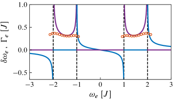
Figure 2: Comparison between the exact decay rate given by the imaginary part of the complex poles of $G_{e}$ (orange circles) and the Markovian decay rate (purple line) as a function of the emitter’s bare frequency. We also plot the Markovian Lamb shift (blue line). The dashed vertical lines mark the position of the bath’s band edges. The parameters of the system are $\delta=0.5$, $g=0.4J$.

To compute the integral in Eq. (4.9), we can use residue integration closing the contour of integration in the lower half of the complex plane. As a first approximation, one can assume that $\Sigma_{e}$ is small and varies little in the neighbourhood of $\omega_{e}$, and substitute $z$ by $\omega_{e}$ in its argument. This is essentially the same as the Markovian approximation, since the Green’s function has then a single pole at $\omega_{e}+\Sigma_{e}(\omega_{e}+i0^{+})$ and the evolution is given by $\psi_{e}(t)=e^{-i[\omega_{e}+\Sigma_{e}(\omega_{e}+i0^{+})]t}$. One can readily identify $\delta\omega_{e}\equiv\operatorname{Re}\Sigma_{e}(\omega_{e}+i0^{+})$ as a shift of the emitter’s frequency, known as the Lamb shift, and $\Gamma_{e}\equiv-2\operatorname{Im}\Sigma_{e}(\omega_{e}+i0^{+})$ as the decay rate of the emitter’s excited state, which can be expressed in terms of the bath’s density of modes $D(E)$ at emitter frequency as $\Gamma_{e}=\pi g^{2}D(\omega_{e})$ (Fermi’s golden rule). They are plotted in Fig. 2. Note that $\Gamma_{e}$ is nonzero only inside the bath’s band regions, while the $\delta\omega_{e}$ is nonzero only outside them. This result corresponds to the basic expectation that if the frequency of the emitter is within the bath’s energy bands of allowed modes, the emitter will decay exponentially with a decay rate given by Fermi’s golden rule. On the contrary, if the emitter’s frequency lays outside the bath’s energy bands, it will remain excited.

As we will see next, an exact calculation of the integral yields somewhat different results. It requires choosing a proper contour of integration due to the branch cuts that the Green’s function has along the real axis in the regions where the bands of the bath are defined. A way to do it is to take a detour at the band edges to other Riemann sheets of the function, see Fig. 3. The formula for the Green’s function in the first Riemann sheet $G^{I}_{e}$ is the one we have provided already. Its analytical continuation to the second Riemann sheet $G^{I\!I}_{e}$ can be obtained changing the sign of the square root in the denominator of $\Sigma_{e}$.

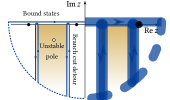
Figure 3: Integration path to compute the dynamics (in blue). Since the Green’s function has branch cuts along the real axis, it is necessary to take a detour to the second Riemann sheet of the function (shaded areas). The dynamics can be split in the contribution from the real poles of the function (black dots), the complex poles (white dot) and the detours taken at the band edges. $G^{I}_{e}$ has no complex poles in the lower half complex plane thus we only have to consider them in the band regions where we go to the second Riemann sheet. Real poles only appear in the band gap regions.

According to this procedure the dynamics can be split in contributions of three different kinds:

$$\psi_{e}(t)=\mathop{{\sum}}_{z_{\mathrm{BS}}}R(z_{\mathrm{BS}})e^{-iz_{\mathrm{BS}}t}+\mathop{{\sum}}_{z_{\mathrm{UP}}}R(z_{\mathrm{UP}})e^{-iz_{\mathrm{UP}}t}+\mathop{{\sum}}_{j}\psi_{\mathrm{BC},j}(t)\,.$$ (4.11)

The first term accounts for the contribution of real poles of $G_{e}$, the so-called bound states (BS). These are non-decaying solutions of the Schrödinger equation. The second term accounts for the contribution of unstable poles (UP), i.e., complex poles of $G_{e}$. These are solutions that decay exponentially. The residue at both the real and complex poles can be computed as $R(z_{0})=[1-\Sigma^{\prime}_{e}(z_{0})]^{-1}$, where $\Sigma^{\prime}_{e}(z_{0})$ denotes the first derivative of the appropriate function $\Sigma^{I}_{e}(z)$ or $\Sigma^{I\!I}_{e}(z)$. It can be interpreted as the overlap between the initial wavefunction and these solutions. Finally, we should subtract the detours taken due to the branch cuts. Their contribution can be computed as

$$\psi_{\mathrm{BC},j}(t)=\frac{\pm 1}{2\pi}\int_{0}^{\infty}d\mkern-1.5mu{y}\,\left[G^{I}_{e}(x_{j}-iy)-G^{I\!I}_{e}(x_{j}-iy)\right]e^{-i(x_{j}-iy)t}\,,$$ (4.12)

with $x_{j}\in\{\pm 2J,\pm 2|\delta|J\}$. The sign has to be chosen positive if when going from $x_{j}+0^{+}$ to $x_{j}-0^{+}$ the integration goes from the first to the second Riemann sheet, and negative if it is the other way around.

We can now point out several differences between the exact dynamics and the dynamics within the Markovian approximation. To begin with, the actual decay rate does not diverge at the band edges, but acquires a finite value, contrary to the Markovian prediction, see Fig. 2. Furthermore, the actual decay is not purely exponential, as the BC contributions decay algebraically $\sim t^{-3}$ [114] (see appendix 4.C). In Fig. 4(a) it is shown an example of this subexponential decay when $\omega_{e}$ is placed at the lower band edge of the bath’s spectrum. Another difference between the Markovian and the exact result is the fractional decay that the emitter experiences when its frequency lays outside the bath’s energy bands . This is due to the emergence of photon bound states which localize the photon around the emitter [115, 116, 117]. For example, in Fig 4(b) we show the dynamics of an emitter with frequency in the middle of the band gap ($\omega_{e}=0$). It remains in the excited state with a long time limit given by the residue at $z_{\mathrm{BS}}=0$, $\lim_{t\to\infty}|\psi_{e}(t)|^{2}=|R(0)|^{2}=\left[1+g^{2}/(4J^{2}\lvert\delta\rvert)\right]^{-2}$.

Figure 4: (a) Sub-exponential decay for a system with parameters: $\omega_{e}=-2J$, $\delta=0.5$ and $g=0.2J$. We plot the squared absolute value of the decaying part of the dynamics $D(t)=\psi_{e}(t)-\sum_{z_{\mathrm{BS}}}R(z_{\mathrm{BS}})e^{-iz_{\mathrm{BS}}t}$. (b) Fractional decay for different values of the dimerization parameter. The rest of parameters of the system are $\omega_{e}=0$ and $g=0.4J$. As the band gap closes ($\delta\to 0$) the decay becomes stronger. The dashed lines mark the value of $|R(0)|^{2}$

These photon bound states are not unique to this particular bath [118]. However, the BSs appearing in the present topological waveguide bath have some distinctive features with no analogue in other systems, and deserve special attention. As we will see later, they play a crucial role in the coherent evolution of many emitters. We can find their energy and wavefunction solving the secular equation $H\lvert\Psi_{\mathrm{BS}}\rangle=E_{\mathrm{BS}}\lvert\Psi_{\mathrm{BS}}\rangle$, with $E_{\mathrm{BS}}$ outside the band regions and $\lvert\Psi_{\mathrm{BS}}\rangle$ in the form of Eq. (4.8) with time-independent coefficients. Without loss of generality we assume that the emitter couples to sublattice $A$ at the $j=0$ cell. After some algebra, one finds that the energy of the BS is given by the pole equation $E_{\mathrm{BS}}=\omega_{e}+\Sigma_{e}(E_{\mathrm{BS}})$. Irrespective of the values of $\omega_{e}$ or $g$, there are always three solutions to this equation. This is because the self-energy diverges in all band edges (see Fig. 2), which guarantees finding a BS in each of the band gaps. The wavefunction amplitudes can be obtained as

$$\psi_{jA}=\frac{gE_{\mathrm{BS}}\psi_{e}}{2\pi}\int_{-\pi}^{\pi}d\mkern-1.5mu{k}\,\frac{e^{ikj}}{E_{\mathrm{BS}}^{2}-\omega_{k}^{2}}\,,$$ (4.13)

$$\psi_{jB}=\frac{g\psi_{e}}{2\pi}\int_{-\pi}^{\pi}d\mkern-1.5mu{k}\,\frac{\omega_{k}e^{i(kj-\phi_{k})}}{E_{\mathrm{BS}}^{2}-\omega_{k}^{2}}\,,$$ (4.14)

where $\psi_{e}$ is a constant obtained from the normalization condition that is directly related with the long-time population of the excited state in spontaneous emission.

Figure 5: Single-photon bound states for a single emitter with transition frequencies $\omega_{e}=2.2J$ (upper row), $\omega_{e}=0$ (middle row) and $\omega_{e}=-2.2J$ (bottom row). Only the dominant bound state is plotted for each case. Rest of parameters: $g=0.4J$, $\delta=0.2$, and $w=0.6J$ for the disordered cases

They are plotted in the left column of Fig. 5. From Eqs. (4.13) and (4.14) we can extract several properties of the spatial wavefunction distribution. On the one hand, above or below the bands ($|E_{\mathrm{BS}}|>2J$, upper and lower band gaps) the largest contribution to the integrals is that of $k=0$. Thus, the amplitude of the wavefunction in any sublattice $\psi_{j\alpha}$ has the same sign regardless the unit cell $j$. In the lower (upper) band-gap, the amplitude on the different sublattices has the same (opposite) sign. On the other hand, in the inner band gap ($|E_{\mathrm{BS}}|<2|\delta|J$), the main contribution to the integrals is that of $k=\pi$. This gives an extra factor $(-1)^{j}$ to the coefficients $\psi_{j\alpha}$. Furthermore, in any band gap, the amplitudes on the sublattice to which the QE couples are symmetric with respect to the position of the QE, whereas they are asymmetric in the other sublattice, that is, the BSs are chiral. Changing $\delta$ from positive to negative results in a spatial inversion of the BS wavefunction. The asymmetry of the BS wavefunction is more extreme in the middle of the inner band-gap, for $\omega_{e}=0$. At this point the BS has energy $E_{\mathrm{BS}}=0$. If $\delta>0$, its wavefunction is given by $\psi_{jA}=0$ and

$$\psi_{jB}=\begin{dcases}\frac{g\psi_{e}(-1)^{j}}{J(1+\delta)}\left(\frac{1-\delta}{1+\delta}\right)^{j}\,,&j\geq 0\\ 0\,,&j<0\\ \end{dcases}\,,$$ (4.15)

whereas for $\delta<0$ the wavefunction decays for $j<0$, and is strictly zero for $j\geq 0$. Its decay length diverges as $\lambda_{\mathrm{BS}}\sim 1/(2|\delta|)$ when the gap closes. Away from this point, the BS decay length shows the usual behavior for 1D baths $\lambda_{\mathrm{BS}}\sim|\Delta_{\mathrm{edge}}|^{-1/2}$, with $\Delta_{\mathrm{edge}}$ being the smallest detuning between the QE frequency and the band-edges.

The physical intuition behind the appearance of such chiral BS at $E_{\mathrm{BS}}=0$ is that the QE with $\omega_{e}=0$ acts as an effective edge in the middle of the chain, or equivalently, as a boundary between two semi-infinite chains with different topology. In fact, one can show that this chiral BS has the same properties as the edge-state that appears in a semi-infinite SSH chain in the topologically non-trivial phase, for example, inheriting its robustness to disorder. To illustrate it, we study the effect of two types of disorder: one that appears in the cavities’ bare frequencies, and another one that appears in the tunneling amplitudes. The former corresponds to the addition of random diagonal terms to the bath’s Hamiltonian and breaks the chiral symmetry of the original model,

$$H_{B}\to H_{B}+\mathop{{\sum}}_{j}\mathop{{\sum}}_{\alpha=A,B}\epsilon_{j\alpha}c^{\dagger}_{j\alpha}c_{j\alpha}\,,\\$$ (4.16)

while the latter corresponds to the addition of off-diagonal random terms and preserves it,

$$H_{B}\to H_{B}+\mathop{{\sum}}_{j}\left(\epsilon_{j1}c^{\dagger}_{jB}c_{jA}+\epsilon_{j2}c^{\dagger}_{j+1A}c_{jB}+\mathrm{H.c.}\right)\,.$$ (4.17)

We take the coefficients $\epsilon_{j\nu}$, $\nu\in\{A,B,1,2\}$, from a uniform distribution within the range $[-w/2,w/2]$. To prevent changing the sign of the coupling amplitudes between the cavities, $w$ is restricted to $w/2<J(1-|\delta|)$ in the case of off-diagonal disorder.

In the middle (right) column of Fig. 5 we plot the shape of the three BS appearing in our problem for a situation with off-diagonal (diagonal) disorder with $w=0.6J$. There, we observe that while the upper and lower BS get modified for both types of disorder, the chiral BS has the same protection against off-diagonal disorder as a regular SSH edge-state: its energy is pinned at $E_{\mathrm{BS}}=0$ as well as keeping its shape with no amplitude in the sublattice to which the QE couples to. On the contrary, for diagonal disorder the middle BS is not protected any more and may have weight in both sublattices.

Finally, to make more explicit the different behavior with disorder of the middle BS compared to the other ones, we compute their localization length $\lambda_{\mathrm{BS}}$ as a function of the disorder strength $w$ averaging for many realizations. In Fig. 6 we plot both the average value (markers) of $\lambda_{\mathrm{BS}}^{-1}$ and its standard deviation (bars) for the cases of the middle (blue circles) and upper (purple triangles) BSs. Generally, one expects that for weak disorder, states outside the band regions tend to delocalize, while for strong disorder all eigenstates become localized (see, for example, Ref. [56]). In fact, this is the behavior we observe for the upper BS for both types of disorder. However, the numerical results suggest that for off-diagonal disorder the chiral BS never delocalizes (on average). Furthermore, the chiral BS localization length is less sensitive to the disorder strength $w$ manifested in both the large initial plateau as well as the smaller standard deviations compared to the upper BS results.

Figure 6: Inverse BS localization length as a function of the disorder strength $w$ for both diagonal and off-diagonal disorder. The markers correspond to the average value computed with a total of $10^{4}$ instances of disorder, and the error bars mark the value of one standard deviation above and below the average value. The two sets of points are slightly offset along the $x$ axis for better visibility. The two cases shown correspond to $\omega_{e}\simeq 2.06J$ (purple triangles) and $\omega_{e}=0$ (blue circles), which in the case without disorder have the same decay length. The rest of parameters are: $g=0.4J$ and $\delta=0.5$.

4.1.2.  Two emitter dynamics

The next simplest case we can study is that of two QE coupled to the bath. From the master equation (4.4), we can see that if the QEs frequency is in one of the band gaps, the interaction with the bath leads to an effective unitary dynamics governed by the following Hamiltonian:

$$H_{\mathrm{dd}}=J^{\alpha\beta}_{12}\left(\sigma^{1}_{eg}\sigma^{2}_{ge}+\mathrm{H.c.}\right)\,.$$ (4.18)

That is, the bath mediates dipole-dipole interactions between the emitters. One way to understand the origin of these interactions is that the emitters exchange virtual photons through the bath. In fact, these virtual photons are nothing but the photon BS that we have studied in the previous section. Thus, these interactions $J^{\alpha\beta}_{mn}$ inherit many properties of the BSs. For example, the interactions are exponentially localized in space, with a localization length that can be tuned and made large by setting $\omega_{e}$ close to the band-edges, or fixing $\omega_{e}=0$ and letting the middle band gap close, $\delta\to 0$. Moreover, one can also change qualitatively the interactions by moving $\omega_{e}$ to different band gaps: for $|\omega_{e}|>2J$ all the $J^{\alpha\beta}_{mn}$ have the same sign, while for $|\omega_{e}|<2|\delta|J$ they alternate sign as $x_{mn}$ increases. Also, changing $\omega_{e}$ from positive to negative changes the sign of $J^{AA/BB}_{mn}$, but leaves unaltered $J^{AB/BA}_{mn}$. Furthermore, while $J^{AA/BB}_{mn}$ are insensitive to the bath’s topology, the $J^{AB/BA}_{mn}$ mimic the dimerization of the underlying bath, but allowing for longer range couplings. The most striking regime is reached for $\omega_{e}=0$. In that case $J^{AA/BB}_{mn}$ identically vanish, so the QEs only interact if they are coupled to different sublattices. Furthermore, in such a situation the interactions have a strong directional character, i.e., the QEs only interact if they are in some particular order. Assuming that the first QE at $x_{1}$ couples to sublattice $A$, and the second one at $x_{2}$ couples to $B$, we have

$$J^{AB}_{12}=\begin{cases}\operatorname{sign}(\delta)\frac{g^{2}(-1)^{x_{12}}}{J(1+\delta)}\left(\frac{1-\delta}{1+\delta}\right)^{x_{12}}\,,&\delta\cdot x_{12}>0\\ 0\,,&\delta\cdot x_{12}<0\\ \Theta(\delta)\frac{g^{2}}{J(1+\delta)}\,,&x_{12}=0\end{cases}\,.$$ (4.19)

We can also apply resolvent operator techniques to compute the dynamics of two emitters exactly. It can be shown that the symmetric and antisymmetric combinations $\sigma^{\dagger}_{\pm}=\left(\sigma^{1}_{eg}\pm\sigma^{2}_{eg}\right)/\sqrt{2}$ evolve independently as they couple to orthogonal bath modes [119] (see appendix 4.A). Thus, the two-emitter problem is equivalent to two independent single-emitter problems. Remarkably the self-energies adopt the simple form $\Sigma^{\alpha\beta}_{\pm}=\Sigma_{e}\pm\Sigma^{\alpha\beta}_{mn}$. We can now compute the two-emitter BSs’ energies solving the pole equations $E_{\mathrm{BS},\pm}=\omega_{e}+\Sigma^{\alpha\beta}_{\pm}(E_{\mathrm{BS},\pm})$. However, there are some subtleties which differentiate this problem from the single-emitter problem. Now, the cancellation of divergences in $\Sigma_{\pm}$ at the band edges results in critical values for the emitter transition frequency above (or below) which some bound states cease to exist. For example, for two emitters in the $AB$ configuration, in the symmetric subspace we have that the lower bound state ($E_{\mathrm{BS},+}<-2J$) always exists, while the upper bound state ($E_{\mathrm{BS},+}>2J$) exists only for $\omega_{e}>\omega_{\mathrm{crit}}$,

$$\omega_{\mathrm{crit}}=2J-\frac{g^{2}(2x_{12}+1-\delta)}{2J(1-\delta^{2})}\,.$$ (4.20)

For the middle bound state, there are two possibilities: either the divergence vanishes at $-2|\delta|J$, in which case the bound state will exist for $\omega_{e}>\omega_{\mathrm{crit}}$, or the divergence vanishes at $2|\delta|J$, then the middle bound state exists for $\omega_{e}<\omega_{\mathrm{crit}}$. In both cases $\omega_{\mathrm{crit}}$ takes the same form

$$\omega_{\mathrm{crit}}=(-1)^{x_{12}}\left\{2\delta J+\frac{g^{2}[(2x_{12}+1)\delta-1]}{2J(1-\delta^{2})}\right\}\,.$$ (4.21)

The situation in the antisymmetric subspace can be readily understood realizing that $\operatorname{Re}\Sigma^{\alpha\beta}_{-}(z)=-\operatorname{Re}\Sigma^{\alpha\beta}_{+}(-z)$, which implies that if $E_{\mathrm{BS},+}$ is a solution of the pole equation for $\Sigma^{\alpha\beta}_{+}$ for a particular value of $\omega_{e}$, then $E_{\mathrm{BS},-}=-E_{\mathrm{BS},+}$ is a solution of the pole equation for $\Sigma^{\alpha\beta}_{-}$ for the opposite value of $\omega_{e}$. Fig. 7 summarizes at a glance the different possibilities and the dependence on the bath’s topology.

The physical intuition behind this phenomenon is the following: when bringing close together two emitters, their respective single-emitter bound states hybridize forming (anti)symmetric superpositions which have energies above and below the single emitter bound state energy. Back in the localized basis the splitting of the bound state energies corresponds to the “hopping” of the photon, i.e., an effective dipole-dipole interaction between the emitters, $J^{\alpha\beta}_{12}=(E_{\mathrm{BS},+}-E_{\mathrm{BS},-})/2$. If this splitting is very strong, it may happen that one of the two bound states merges into the bulk bands. Then it is not possible to rewrite the low-energy Hamiltonian as an effective dipole-dipole interaction [120]. In Fig. 8 we show the exact value of the interaction constant and compare it with the Markovian result (4.19). Apart from small deviations when the gap closes for $\delta\to 0$, it is important to highlight that the directional character agrees perfectly in both cases.

Figure 7: Exact energies for the symmetric (continuous line) and antisymmetric (dashed line) bound states for a system with parameters: $g=0.8J$, and $\delta=0.5$ (right) or $\delta=-0.5$ (left). The two emitters are in the $AB$ configuration coupled to the same unit cell, $x_{12}=0$. The grey areas mark the span of the bath’s energy bands.

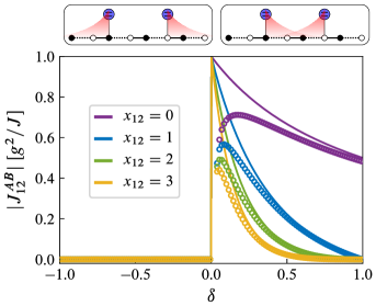
Figure 8: Effective dipolar coupling as given by the BSs energy difference (dots), and the Markovian approximation (4.19) (lines) as a function of the dimerization constant. The rest of parameters are $\omega_{e}=0$ and $g=0.4J$. The schematics above show the shape of the bound states in the topological (right) and trivial (left) phases. The situation for the $BA$ configuration is the same, reversing the role of $\delta$.

When the QEs frequency is resonant with one of the bath’s bands, the bath typically induces non-unitary dynamics in the emitters. However, when many QEs couple to the bath there are situations in which the interference between their emission may enhance or suppress (even completely) the decay of certain states. This phenomenon is known as super/subradiance [121], respectively. Let us illustrate this effect with two QEs: In that case, the decay rate of a symmetric/antisymmetric combination of excitations is $\Gamma_{e}\pm\Gamma^{\alpha\beta}_{12}$. When $\Gamma^{\alpha\beta}_{12}=\pm\Gamma_{e}$, these states decay at a rate that is either twice the individual one or zero. In this latter case they are called perfect subradiant or dark states.

In standard one-dimensional baths $\Gamma_{12}(\omega_{e})=\Gamma_{e}(\omega_{e})\cos\big{(}k(\omega_{e})|x_{mn}|\big{)}$, so the dark states are such that the wavelength of the photons involved, $k(\omega_{e})$, allows for the formation of a standing wave between the QEs when both try to decay, i.e., when $k(\omega_{e})|x_{mn}|=n\pi$, with $n\in\mathbb{N}$. Thus, the emergence of perfect super/subradiant states solely depends on the QE frequency $\omega_{e}$, bath energy dispersion $\omega_{k}$, and their relative position $x_{mn}$, which is the common intuition for this phenomenon. This common wisdom gets modified in the topological bath that we have considered, where we find situations in which, for the same values of $x_{mn}$, $\omega_{k}$ and $\omega_{e}$, the induced dynamics is very different depending on the sign of $\delta$. In particular, when two QEs couple to the $A$ and $B$ sublattice respectively, the collective decay reads:

$$\Gamma^{AB}_{12}(\omega_{e})=\Gamma_{e}\operatorname{sign}(\omega_{e})\cos\big{(}k(\omega_{e})x_{12}-\phi(\omega_{e})\big{)}\,,$$ (4.22)

which depends both on the photon wavelength mediating the interaction

$$k(\omega_{e})=\arccos\left(\frac{\omega_{e}^{2}-2J^{2}(1+\delta^{2})}{2J^{2}(1-\delta^{2})}\right)\,,$$ (4.23)

an even function of $\delta$, and on the phase $\phi(\omega_{e})\equiv\phi(k(\omega_{e}))$, which is sensitive to the sign of $\delta$. This $\phi$-dependence enters through the system-bath coupling when rewriting the interaction Hamiltonian $H_{I}$ [Eq. (4.3)] in terms of the eigenoperators $u_{k},l_{k}$ (see appendix 4.A). Thus, even though the sign of $\delta$ does not play a role in the properties of an infinite bath, when the QEs couple to it, the bath embedded between them is different for $\delta\gtrless 0$, making the two situations inequivalent.

Using Eq. (4.22), we find that the detunings at which perfect super/subradiant states appear satisfy $k(\omega_{s})x_{12}-\phi(\omega_{s})=n\pi$, $n\in\mathbb{N}$. They come in pairs: If $\omega_{s}$ corresponds to a superradiant (subradiant) state in the upper band, $-\omega_{s}$ corresponds to a subradiant (superradiant) state in the lower band. In particular, it can be shown that when $\delta<0$, the previous equation has solutions for $n=0,\dots,x_{12}$, while if $\delta>0$, the equation has solutions for $n=0,\dots,x_{12}+1$. Besides, the detunings, $\omega_{s}$ at which the subradiant states appear also satisfy that $J_{12}^{AB}(\omega_{s})\equiv 0$, which guarantees that these subradiant states survive even in the non-Markovian regime with a correction due to retardation which is small as long as $x_{12}\Gamma_{e}(\omega_{e})/(2|v_{g}(\omega_{e})|)\ll 1$ [$v_{g}(\omega_{e})$ is the group velocity of the photons in the bath at frequency $\omega_{e}$] [119]. Apart from inducing different decay dynamics, these different conditions for super/subradiance at fixed $\omega_{e}$ also translate in different reflection/transmission coefficients when probing the system through photon scattering, as we show in the next section.

4.2.  Single-photon scattering

Here, we study the case when the emitter frequencies are resonant with one of the bands. We will see how for a single emitter coupled to both the $A$ and $B$ cavities inside a unit cell there is a $\delta$-dependent Lamb-Shift that can be detected in single-photon scattering experiments. Also, we will see how the different super/subradiant states for $\pm\delta$ lead to different behavior when a single photon scatters off two QEs.

4.2.1.  Scattering formalism

The scattering properties of a single photon impinging into one or several QEs in the ground state can be obtained from the scattering eigenstates, which are solutions of the secular equation $H\lvert\Psi_{k}\rangle=\pm\omega_{k}\lvert\Psi_{k}\rangle$ (the sign depends on the band we are probing). First, let us assume that a single emitter couples to the $A$ sublattice at the $x_{1}$ unit cell. We use the ansatz

$$\lvert\Psi_{k}\rangle=\begin{cases}\psi^{\mathrm{in}}_{k}\lvert k\rangle+\psi^{\mathrm{out}}_{-k}\lvert-k\rangle\,,&j<x_{1}\\ \psi^{\mathrm{out}}_{k}\lvert k\rangle+\psi^{\mathrm{in}}_{-k}\lvert-k\rangle\,,&j\geq x_{1}\end{cases}\,,$$ (4.24)

where $\lvert\pm k\rangle=u^{\dagger}_{\pm k}\lvert\mathrm{vac}\rangle$ or $\lvert\pm k\rangle=l^{\dagger}_{\pm k}\lvert\mathrm{vac}\rangle$, depending on the band we are probing ($u_{k}$ and $l_{k}$ are the eigenmodes of the SSH model, see section 2.1). For a schematic representation of $\lvert\Psi_{k}\rangle$ see Fig. 9.

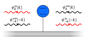
Figure 9: Schematic picture of a scattering eigenstate and the different amplitudes involved. The QE divides the space in left and right regions. Incoming modes are those that propagate towards the emitter (red), while outgoing modes are those that propagate away from the emitter (black).

The coefficients of the scattering eigenstate in position representation are then

$$\psi_{jA} =\pm\begin{cases}\psi_{k}^{\mathrm{in}}e^{i(kj+\phi_{k})}+\psi_{-k}^{\mathrm{out}}e^{-i(kj+\phi_{k})}\,,&j\leq x_{1}\\ \psi_{k}^{\mathrm{out}}e^{i(kj+\phi_{k})}+\psi_{-k}^{\mathrm{in}}e^{-i(kj+\phi_{k})}\,,&j\geq x_{1}\end{cases}\,,$$ (4.25)

$$\psi_{jB} =\begin{cases}\psi_{k}^{\mathrm{in}}e^{ikj}+\psi_{-k}^{\mathrm{out}}e^{-ikj}\,,&j<x_{1}\\ \psi_{k}^{\mathrm{out}}e^{ikj}+\psi_{-k}^{\mathrm{in}}e^{-ikj}\,,&j\geq x_{1}\end{cases}\,.$$ (4.26)

The matching condition at the emitter position

$$\psi_{k}^{\mathrm{in}}e^{i(kx_{1}+\phi_{k})}+\psi_{-k}^{\mathrm{out}}e^{i(kx_{1}+\phi_{k})}=\psi_{k}^{\mathrm{out}}e^{i(kx_{1}+\phi_{k})}+\psi_{-k}^{\mathrm{in}}e^{i(kx_{1}+\phi_{k})}\,,$$ (4.27)

together with the secular equation

$$\begin{cases}\omega_{e}\psi_{e}+g\psi_{x_{1}A}=\pm\omega_{k}\psi_{e}\,,\\ g\psi_{e}+-J(1+\delta)\psi_{x_{1}B}-J(1-\delta)\psi_{x_{1}-1B}=\pm\omega_{k}\psi_{x_{1}A}\,,\end{cases}$$ (4.28)

$$\Rightarrow-J(1+\delta)\psi_{x_{1}B}-J(1-\delta)\psi_{x_{1}-1B}=\left(\pm\omega_{k}-\frac{g^{2}}{\Delta_{k}}\right)\psi_{x_{1}A}\,,$$ (4.29)

where we have defined $\Delta_{k}\equiv\pm\omega_{k}-\omega_{e}$, allow us to write a linear relation between the wave amplitudes on the left of the emitter and those on the right as

$$\begin{pmatrix}\psi_{k}^{\mathrm{out}}\\ \psi_{-k}^{\mathrm{in}}\end{pmatrix}=T\begin{pmatrix}\psi_{k}^{\mathrm{in}}\\ \psi_{-k}^{\mathrm{out}}\end{pmatrix}\,,$$ (4.30)

where the transfer matrix $T$ is

$$T_{A}=\begin{pmatrix}1\pm\dfrac{g^{2}}{i2\Delta_{k}J(1-\delta)\sin(k+\phi_{k})}&\dfrac{\pm g^{2}e^{-i2(kx_{1}+\phi_{k})}}{i2\Delta_{k}J(1-\delta)\sin(k+\phi_{k})}\\[9.00002pt] \dfrac{\mp g^{2}e^{i2(kx_{1}+\phi_{k})}}{i2\Delta_{k}J(1-\delta)\sin(k+\phi_{k})}&1\mp\dfrac{g^{2}}{i2\Delta_{k}J(1-\delta)\sin(k+\phi_{k})}\end{pmatrix}\,.$$ (4.31)

Similarly, if the emitter couples to the $B$ sublattice at the $x_{1}$ unit cell we have

$$T_{B}=\begin{pmatrix}1\mp\dfrac{g^{2}}{i2\Delta_{k}J(1+\delta)\sin(\phi_{k})}&\dfrac{\mp g^{2}e^{-i2kx_{1}}}{i2\Delta_{k}J(1+\delta)\sin(\phi_{k})}\\[10.00002pt] \dfrac{\pm g^{2}e^{i2kx_{1}}}{i2\Delta_{k}J(1+\delta)\sin(\phi_{k})}&1\pm\dfrac{g^{2}}{i2\Delta_{k}J(1+\delta)\sin(\phi_{k})}\end{pmatrix}\,.$$ (4.32)

From the transfer matrix we can compute the scattering matrix $S$, which relates the asymptotic incoming modes with the outgoing modes:

$$\begin{pmatrix}\psi_{k}^{\mathrm{out}}\\ \psi_{-k}^{\mathrm{out}}\end{pmatrix}=S\begin{pmatrix}\psi_{k}^{\mathrm{in}}\\ \psi_{-k}^{\mathrm{in}}\end{pmatrix}\,,$$ (4.33)

with

$$S=\begin{pmatrix}t_{11}-\dfrac{t_{12}t_{21}}{t_{22}}&\dfrac{t_{12}}{t_{22}}\\[10.00002pt] -\dfrac{t_{21}}{t_{22}}&\dfrac{1}{t_{22}}\end{pmatrix}\equiv\begin{pmatrix}t_{L}&r_{R}\\ r_{L}&t_{R}\end{pmatrix}\,.$$ (4.34)

Here, $t_{ij}$ denote the matrix elements of the transfer matrix, while $t_{L/R}$ and $r_{L/R}$ denote the matrix elements of the scattering matrix. They correspond to the transmission and reflection probability amplitudes for a wave coming from the left/right.

If evolution is unitary, that is, there are no photon losses, $S^{\dagger}S=SS^{\dagger}=I$, which implies $|t_{L}|^{2}+|r_{L}|^{2}=|t_{R}|^{2}+|r_{R}|^{2}=1$ and $|t_{L}|^{2}+|r_{R}|^{2}=|t_{R}|^{2}+|r_{L}|^{2}=1$. Therefore, $|t_{L}|=|t_{R}|$ and $|r_{L}|=|r_{R}|$. Furthermore if the system is time-reversal symmetric ($H$ is real), as is the case in our model, the scattering is reciprocal, i.e., $t_{L}=t_{R}\equiv t$. To see this, let us consider the scattering eigenstate with amplitudes $(\psi_{k}^{\mathrm{in}},\psi_{-k}^{\mathrm{in}},\psi_{k}^{\mathrm{out}},\psi_{-k}^{\mathrm{out}})=(1,0,t_{L},r_{L})$, and call it $\lvert\Psi_{k,L}\rangle$. Then, its complex conjugate is also a scattering eigenstate with the same energy and so is the linear combination $(1/t_{L}^{*})\lvert\Psi_{k,L}\rangle^{*}-(r_{L}^{*}/t_{L}^{*})\lvert\Psi_{k,L}\rangle$, which has coefficients $\left(0,1,-r_{L}^{*}t_{L}/t_{L}^{*},t_{L}\right)$, but this must be the scattering eigenstate with coefficients $(0,1,r_{R},t_{R})$.

The scattering coefficients for the many-emitter case can be readily obtained noting that if we label the emitters with an increasing index from left to right, the fields on the right of the $m$th emitter are those on the left of the $(m+1)$th emitter. Thus, the transfer matrix of the entire system can be written as the product of single-emitter transfer matrices $T=T_{N_{e}}T_{N_{e}-1}\dots T_{1}$ ($N_{e}$ is the number of emitters) and from it one can compute the scattering matrix of the entire system.

4.2.2.  Scattering off one and two emitters

For a single emitter, we find the same transmission coefficient regardless the sublattice to which the emitter is coupled

$$t=\frac{2J^{2}(1-\delta^{2})\Delta_{k}\sin(k)}{2J^{2}(1-\delta^{2})\Delta_{k}\sin(k)\mp ig^{2}\omega_{k}}\,.$$ (4.35)

A well-known feature for this type of system is the perfect reflection ($\lvert r\rvert^{2}=1\Leftrightarrow\lvert t\rvert^{2}=0$) when the frequency of the incident photon matches exactly that of the QE [122]. This can be seen in Fig. 10(a) as a full dip in the transmission probability at $\Delta_{k}=0$. The dip has a bandwidth determined by the individual decay rate $\Gamma_{e}$. Besides, it also shows the vanishing of the transmission at the band edges. Since there is no dependence on the sign of $\delta$, the scattering in this configuration is insensitive to the bath’s topology.

A more interesting situation occurs when a single emitter couples to both the $A$ and $B$ cavities in a single cell. We choose the coupling constants $g\alpha$ and $g(1-\alpha)$, such that we can interpolate between the cases where the QE couples only to sublattice $A$ ($\alpha=1$) or $B$ ($\alpha=0$). Using the same ansatz as in the previous case, we find

$$t=\frac{2iJ(1-\delta)\sin(k)\left[J(1+\delta)\Delta_{k}-g^{2}\alpha(1-\alpha)\right]}{2iJ^{2}(1-\delta^{2})\Delta_{k}\sin(k)+g^{2}\omega_{k}\left[2\alpha(1-\alpha)(e^{-i\phi_{k}}\mp 1)\pm 1\right]}\,.$$ (4.36)

Now, for $0<\alpha<1$, the transmission is different for $\pm\delta$. In Fig. 10(a) we plot this formula for $\delta=\pm 0.3$, and show that the transmission dip gets shifted. This is due to a $\delta$-dependent Lamb-Shift $\delta\omega_{e}=g^{2}\alpha(1-\alpha)/\left[J(1+\delta)\right]$. Notice that Eq. (4.36) is invariant under the transformation $\alpha\to 1-\alpha$.

For two emitters coupled equally to the bath at unit cells $x_{1}$ and $x_{2}$, in the $AB$ configuration, we find

$$t=\frac{\left[2J^{2}(1-\delta^{2})\Delta_{k}\sin(k)\right]^{2}}{g^{4}\omega^{2}_{k}e^{i2\left(kx_{12}-\phi_{k}\right)}-\left[g^{2}\omega_{k}\pm 2iJ^{2}(1-\delta^{2})\Delta_{k}\sin(k)\right]^{2}}\,,$$ (4.37)

whose squared absolute value is plotted in Fig. 10(b) for $\delta=\pm 0.5$. The difference between bath in the topological and trivial phases is more pronounced than in the single-emitter case, since now the transmission is qualitatively different in each case: While the case with $\delta>0$ features a single transmission dip at the QEs frequency, for $\delta<0$, the transmission dip is followed by a window of frequencies with perfect photon transmission, i.e., $\lvert t\rvert^{2}=1$. We can understand this behavior realizing that a single photon only probes the (anti)symmetric states in the single excitation subspace $\lvert S\rangle/\lvert A\rangle$, with the following energies renormalized by the bath, $\omega_{S/A}=\omega_{e}\pm J^{AB}_{12}$, and linewidths $\Gamma_{S/A}=\Gamma_{e}\pm\Gamma_{12}$. For the parameters chosen, it can be shown that for $\delta>0$ the QEs are in a perfect super/subradiant configuration in which one of the states decouples while the other has a $2\Gamma_{e}$ decay rate. Thus, at this configuration, the two QEs behave like a single two-level system with an increased linewidth. On the other hand, when $\delta<0$, both the (anti)symmetric states are coupled to the bath, such that the system is analogous to a V-type system where perfect transmission occurs for an incident frequency $\pm\omega_{\mathrm{EIT}}=\left(\omega_{S}\Gamma_{A}-\omega_{A}\Gamma_{S}\right)/(\Gamma_{A}-\Gamma_{S})$ [123]

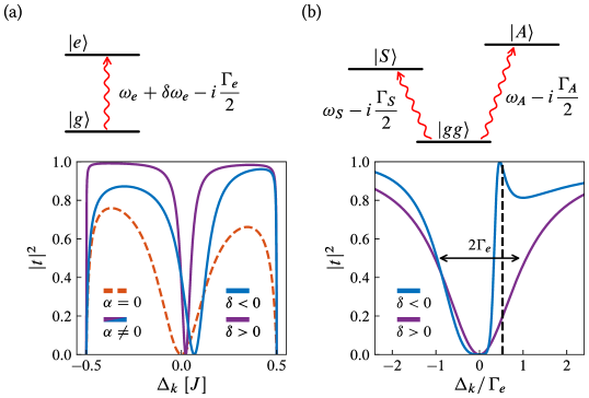
Figure 10: Relevant level structure and transmission probability for a single photon scattering off (a) one QE coupled to both $A$ and $B$ cavities inside a unit cell, (b) two QEs in an $AB$ configuration separated a distance of $x_{12}=2$ unit cells; $\lvert gg\rangle=\lvert g\rangle_{1}\lvert g\rangle_{2}$ denotes the common ground state, while $\lvert S/A\rangle=\left(\lvert e\rangle_{1}\lvert g\rangle_{2}\pm\lvert g\rangle_{1}\lvert e\rangle_{2}\right)/\sqrt{2}$ denotes the (anti)symmetric excited state combination of the two QEs. The parameters in (a) are $g=0.4J$, $\delta=\pm 0.5$, $\omega_{e}=1.5J$, and $\alpha=0$ or $\alpha=0.3$. The dashed orange line corresponds to the case where the emitter couples to a single sublattice ($\alpha=0,1$), it does not depend on the sign of $\delta$. The parameters in (b) are $g=0.1J$, $\delta=\pm 0.5$, and $\omega_{e}\simeq 1.65J$, for which the two QEs are in a subradiant configuration if $\delta>0$. The black dashed line marks the value of $\omega_{\mathrm{EIT}}$.

4.3.  Many emitters: effective spin models

One of the main interests of having a platform with BS-mediated interactions is to investigate spin models with long-range interactions [124, 125]. The study of these models has become an attractive avenue in quantum simulation because long-range interactions are the source of non-trivial many-body phases [126] and dynamics [127], and are also very hard to treat classically.

Let us now investigate how the shape of the QE interactions inherited from the topological bath translate into different many-body phases at zero temperature as compared to those produced by long-range interactions appearing in other setups such as trapped ions [126, 127], or standard waveguide setups. For that, we consider having $N_{e}$ emitters equally spaced and alternatively coupled to the $A/B$ lattice sites. After eliminating the bath, and adding a collective field with amplitude $\mu$ to control the number of spin excitations, the dynamics of the emitters (spins) is effectively given by:

$$H_{\mathrm{spin}}=\mathop{{\sum}}_{m,\,n}J^{AB}_{mn}\left(\sigma_{eg}^{m,A}\sigma_{ge}^{n,B}+\mathrm{H.c.}\right)-\frac{\mu}{2}\mathop{{\sum}}_{n}\left(\sigma_{z}^{n,A}+\sigma_{z}^{n,B}\right)\,,$$ (4.38)

denoting by $\sigma_{\nu}^{n,\alpha}$, $\nu=x,y,z$, the corresponding Pauli matrix acting on the $\alpha\in\{A,B\}$ site in the $n$th unit cell. The $J^{\alpha\beta}_{mn}$ are the spin-spin interactions derived in the previous subsection, whose localization length, denoted by $\xi$, and functional form can be tuned through system parameters such as $\omega_{e}$.

For example, when the lower (upper) BS mediates the interaction, the $J^{\alpha\beta}_{mn}$ has negative (alternating) sign for all sites, similar to the ones appearing in standard waveguide setups. When the range of the interactions is short (nearest neighbor), the physics is well described by the ferromagnetic XY model with a transverse field [128], which goes from a fully polarized phase when $|\mu|$ dominates to a superfluid one in which spins start flipping as $|\mu|$ decreases. In the case where the interactions are long-ranged the physics is similar to that explained in Ref. [126] for power-law interactions ($\propto 1/r^{3}$). The longer range of the interactions tends to break the symmetry between the ferro/antiferromagnetic situations and leads to frustrated many-body phases. Since similar interactions also appear in other scenarios (standard waveguides or trapped ions), we now focus on the more different situation where the middle BS at $\omega_{e}=0$ mediates the interactions, such that the coefficients $J^{AB}_{mn}$ have the form of Eq. (4.19).

In that case, the Hamiltonian $H_{\mathrm{spin}}$ of Eq. (4.38) is very unusual: i) spins only interact if they are in different sublattices, i.e., the system is bipartite ii) the interaction is chiral in the sense that they interact only in case they are properly sorted, i.e., the one in lattice $A$ to the left/right of that in lattice $B$, depending on the sign of $\delta$. Note that $\delta$ also controls the interaction length $\xi$. In particular, for $|\delta|=1$ the interaction only occurs between nearest neighbors, whereas for $\delta\to 0$, the interactions become of infinite range. These interactions translate into a rich phase diagram as a function of $\xi$ and $\mu$, which we plot in Fig. 11 for a small chain with $N_{e}=20$ emitters (obtained with exact diagonalization). Let us guide the reader into the different parts:

1. The region with maximum average magnetization (in white) corresponds to the regimes where $\mu$ dominates such that all spins are aligned upwards.

2. Now, if we decrease $\mu$ from this fully polarized phase in a region where the localization length is short, i.e., $\xi\approx 0.1$, we observe a transition into a state with zero average magnetization. This behavior can be understood because in that short-range limit $J^{AB}_{mn}$ only couples nearest neighbor $AB$ sites, but not $BA$ sites as shown in the scheme of the lower part of the diagram for $\delta>0$ (the opposite is true for $\delta<0$). Thus, the ground state is a product of nearest neighbor singlets (for $J>0$) or triplets (for $J<0$). This state is usually referred to as Valence-Bond Solid in the condensed matter literature [129]. Note, the difference between $\delta\gtrless 0$ is the presence (or not) of uncoupled spins at the edges.

3. However, when the bath allows for longer range interactions ($\xi>1$), the transition from the fully polarized phase to the phase of zero magnetization does not occur abruptly but passing through all possible intermediate values of the magnetization. Besides, we also plot in Fig. 12 the spin-spin correlations along the $x$ and $z$ directions (note the symmetry in the $xy$ plane) for the case of $\mu=0$ to evidence that a qualitatively different order appears as $\xi$ increases. In particular, we show that the spins align along the $x$ direction with a double periodicity, which we can pictorially represent by $\lvert{\uparrow}{\uparrow}{\downarrow}{\downarrow}{\uparrow}{\uparrow}\dots\rangle_{x}$, and that we call double Néel order states. Such orders have been predicted as a consequence of frustration in classical and quantum spin chains with competing nearest and next-nearest neighbour interactions [130, 131, 132], introduced to describe complex solid state systems such as multiferroic materials [133]. In our case, this order emerges in a system which has long-range interactions but no frustration as the system is always bipartite regardless the interaction length.

To gain analytical intuition of this regime, we take the limit $\xi\rightarrow\infty$, where the Hamiltonian (4.38) reduces to

$$H^{\prime}_{\mathrm{spin}}=UH_{\mathrm{spin}}U^{\dagger}\simeq J(S^{+}_{A}S^{-}_{B}+\mathrm{H.c.})\,,$$ (4.39)

where $S^{+}_{A/B}=\sum_{n}\sigma^{n,A/B}_{eg}$, and the unitary transformation $U=\prod_{n\in\mathbb{Z}_{\mathrm{odd}}}\sigma^{n,A}_{z}\sigma^{n,B}_{z}$ is used to cancel the alternating signs of $J^{AB}_{mn}$. Equality in Eq. (4.39) occurs for a system with periodic boundary conditions, while for finite systems with open boundary conditions some corrections have to be taken into account due to the fact that not all spins in one sublattice couple to all spins in the other but only to those to their right/left depending on the sign of $\delta$. The ground state is symmetric under (independent) permutations in $A$ and $B$. In the thermodynamic limit we can apply mean field theory, which predicts symmetry breaking in the spin $xy$ plane. For instance, if $J<0$ and the symmetry is broken along the spin direction $x$, the spins will align so that $\langle(S^{x}_{A})^{2}\rangle=\langle(S^{x}_{B})^{2}\rangle=\langle S^{x}_{A}S^{x}_{B}\rangle=(N_{e}/2)^{2}$, and $\langle S^{x}_{A}\rangle^{2}=\langle S^{x}_{B}\rangle^{2}=(N_{e}/2)^{2}$ .

Since $N_{e}$ is finite in our case, the symmetry is not broken, but it is still reflected in the correlations, so that

$$\langle\sigma^{m,A}_{\nu}\sigma^{n,A}_{\nu}\rangle\simeq\langle\sigma^{m,A}_{\nu}\sigma^{n,B}_{\nu}\rangle\simeq 1/2\,,\quad\nu=x,y\,.$$ (4.40)

In the original picture with respect to $U$, we obtain the double Néel order observed in Fig. 12. As can be understood, the alternating nature of the interactions is crucial for obtaining this type of ordering. Finally, let us mention that the topology of the bath translates into the topology of the spin chain in a straightforward manner: regardless the range of the effective interactions, the ending spins of the chain will be uncoupled to the rest of spins if the bath is topologically non-trivial.

This discussion shows the potential of the present setup to act as a quantum simulator of exotic many-body phases not possible to simulate with other known setups.

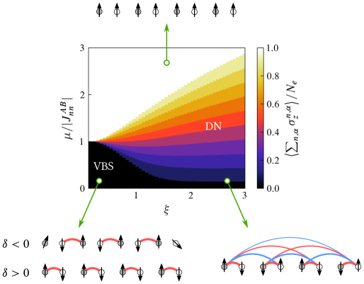
Figure 11: Ground state average polarization obtained by exact diagonalization for a chain with $N_{e}=20$ emitters with frequency tuned to $\omega_{e}=0$ as a function of the chemical potential $\mu$ and the decay length of the interactions $\xi$. The different phases discussed in the text, a Valence-Bond Solid (VBS) and a Double Néel ordered phase (DN) are shown schematically below, on the left and right respectively. Interactions of different sign are marked with links of different color.

Figure 12: Correlations ${C_{\nu}(r)=\langle\sigma^{9}_{\nu}\sigma^{9+r}_{\nu}\rangle-\langle\sigma^{9}_{\nu}\rangle\langle\sigma^{9+r}_{\nu}\rangle}$, $\nu=x,y,z$, [$C_{x}(r)=C_{y}(r)$] for the same system as in Fig. 11 for different interaction lengths, fixing $\mu=0$ (left column). Correlations for different chemical potentials fixing $\xi=5$, darker colors correspond to lower chemical potentials (right column). Note we have defined a single index $r$ that combines the unit cell position and the sublattice index. The yellow dashed line marks the value of $1/2$ expected when the interactions are of infinite range.

4.4.  Summary

We have analyzed the dynamics of a set of quantum emitters (two-level systems) whose ground state-excited state transition couples to the modes of a photonic lattice, which acts as a collective structured bath. For this, we have computed analytically the collective self-energies, which allowed us to use master equations and resolvent operator techniques to study the dynamics of quantum emitters in the Markovian and non-Markovian regimes respectively. The behavior depends fundamentally on whether the transition frequency of the emitters lays in a range of allowed bath modes or a band gap. If the transition frequency is tuned to a band gap we observe the following phenomena:

1. Emergence of chiral bound states, that is, bound states that are mostly localized on the left or right of the emitter depending on the sign of the dimerization constant $\delta$ of the photonic bath. Specifically, when the transition frequency of an emitter lays in the middle of the inner band gap, it acts as a boundary between two photonic lattices with different topology. The resulting bound state has the same properties as a regular topological edge state of the SSH model including the protection against certain types of disorder.

2. An exact calculation reveals that the existence conditions of the bound states for two emitters are different depending on the sign of $\delta$.

3. These bound states give rise to dipolar interactions between the emitters which depend on the topology of the underlying bath if the emitters are coupled to different sublattices. In particular, when the transition frequency of the emitters lays in the middle of the inner band gap, the interactions can be toggled on and off by changing the sign of $\delta$.

When the emitters’ frequency is tuned to the band, the topology of the bath reflects itself in:

1. Different super/subradiant conditions depending on the sign of $\delta$.

2. A $\delta$-dependent Lamb Shift for a single emitter coupled simultaneously to both $A$ and $B$ sublattices. This can be detected as a shift of the transmission dip in single-photon scattering experiments.

3. Different scattering properties for two emitters in an $AB$ configuration depending on the sign of $\delta$. This is a consequence of the different super/subradiant conditions in each phase.

Last, we analyze the zero temperature phases of the effective spin Hamiltonians that can be generated in the many-emitter case after tracing out the bath degrees of freedom. We find that for short-range interactions the emitters realize a valence-bond solid. On the other hand, for long-range interactions, the system becomes gapless and a double Néel order emerges.

Appendices

Appendix 4.A Calculation of the self-energies

To obtain analytical expressions for the self-energies, it is convenient to first express $H_{I}$ in the bath eigenbasis. For this we just have to invert (2.5) to obtain expresions for the local operators $c_{j\alpha}$ in terms of $u_{k}$ and $l_{k}$. Substituting in (4.3) we obtain

$$\begin{split}H_{I}={}&\frac{g}{\sqrt{2N}}\mathop{{\sum}}_{n\in S_{A}}\mathop{{\sum}}_{k}e^{i(kx_{n}+\phi_{k})}(u_{k}+l_{k})\sigma^{n}_{eg}\\ &+\frac{g}{\sqrt{2N}}\mathop{{\sum}}_{n\in S_{B}}\mathop{{\sum}}_{k}e^{ikx_{n}}(u_{k}-l_{k})\sigma^{n}_{eg}+\mathrm{H.c.}\,,\end{split}$$ (4.41)

where $S_{A}$ ($S_{B}$) denotes the set of emitters coupled to the $A$ ($B$) sublattice.

Identifying $H_{0}=H_{S}$ and $V=H_{B}+H_{I}$, using $P=\lvert e\rangle\lvert\mathrm{vac}\rangle\langle\mathrm{vac}\rvert\langle e\rvert$, from Eq. (2.33) we obtain

$$\Sigma_{e}(z)\equiv\langle\mathrm{vac}\rvert\langle e\rvert R(z)\lvert e\rangle\lvert\mathrm{vac}\rangle=\frac{g^{2}}{2N}\mathop{{\sum}}_{k}\left(\frac{1}{z-\omega_{k}}+\frac{1}{z+\omega_{k}}\right)\,.$$ (4.42)

In the thermodynamic limit ($N\to\infty$), the sum can be replaced by an integral, which can be computed easily with the change of variable $e^{ik}=y$ yielding the result shown in Eq. (4.10); the functions $y_{\pm}(z)$ appearing in the expression are the roots of the polynomial

$$p(y)=y^{2}+\left[\frac{2J^{2}(1+\delta^{2})-z^{2}}{J^{2}(1-\delta^{2})}\right]y+1\,.$$ (4.43)

For the two emitter case, we will first show that the (anti)symmetric combinations $\sigma^{\dagger}_{\pm}=\left(\sigma^{1}_{eg}\pm\sigma^{2}_{eg}\right)/\sqrt{2}$ couple to orthogonal bath modes [119]. Substituting $\sigma^{n}_{eq}$, $n=1,2$, in terms of $\sigma^{\dagger}_{\pm}$ in Eq. (4.41), and pairing the terms with opposite momentum, we obtain for the case where the two QEs couple to sublattice $A$

$$H^{AA}_{I}=\frac{g}{\sqrt{N}}\mathop{{\sum}}_{k>0}\mathop{{\sum}}_{\beta=\pm}\sqrt{1+\beta\cos(kx_{12})}(\tilde{u}_{k\beta}+\tilde{l}_{k\beta})\sigma^{\dagger}_{\beta}+\mathrm{H.c.}\,,$$ (4.44)

$$\tilde{u}_{k\pm}=\frac{\left[e^{i(kx_{1}+\phi_{k})}\pm e^{i(kx_{2}+\phi_{k})}\right]u_{k}+\left[e^{-i(kx_{1}+\phi_{k})}\pm e^{-i(kx_{2}+\phi_{k})}\right]u_{-k}}{2\sqrt{1\pm\cos(kx_{12})}}\,,$$ (4.45)

$$\tilde{l}_{k\pm}=\frac{\left[e^{i(kx_{1}+\phi_{k})}\pm e^{i(kx_{2}+\phi_{k})}\right]l_{k}+\left[e^{-i(kx_{1}+\phi_{k})}\pm e^{-i(kx_{2}+\phi_{k})}\right]l_{-k}}{2\sqrt{1\pm\cos(kx_{12})}}\,.$$ (4.46)

Here, $x_{12}=x_{2}-x_{1}$ is the signed distance between the two emitters. For the case where the two QEs are on a different sublattice

$$\begin{split}H^{AB}_{I}=\frac{g}{\sqrt{N}}\mathop{{\sum}}_{k>0}\mathop{{\sum}}_{\beta=\pm}\Big{[}&\sqrt{1+\beta\cos(kx_{12}-\phi_{k})}\,\tilde{u}_{k\beta}\sigma^{\dagger}_{\beta}\\ &\qquad+\sqrt{1-\beta\cos(kx_{12}-\phi_{k})}\,\tilde{l}_{k\beta}\sigma^{\dagger}_{\beta}\Big{]}+\mathrm{H.c.}\,,\end{split}$$ (4.47)

$$\tilde{u}_{k\pm}=\frac{\left[e^{i(kx_{1}+\phi_{k})}\pm e^{ikx_{2}}\right]u_{k}+\left[e^{-i(kx_{1}+\phi_{k})}\pm e^{-ikx_{2}}\right]u_{-k}}{2\sqrt{1\pm\cos(kx_{12}-\phi_{k})}}\,,$$ (4.48)

$$\tilde{l}_{k\pm}=\frac{\left[e^{i(kx_{1}+\phi_{k})}\mp e^{ikx_{2}}\right]l_{k}+\left[e^{-i(kx_{1}+\phi_{k})}\mp e^{-ikx_{2}}\right]l_{-k}}{2\sqrt{1\mp\cos(kx_{12}-\phi_{k})}}\,.$$ (4.49)

The denominators in the definition of $\tilde{u}_{k\pm}$ and $\tilde{l}_{k\pm}$ come from normalization. Importantly, these modes are orthogonal, they satisfy

$$\left[\tilde{u}_{k\alpha},\tilde{u}^{\dagger}_{k^{\prime}\alpha^{\prime}}\right]=\left[\tilde{l}_{k\alpha},\tilde{l}^{\dagger}_{k^{\prime}\alpha^{\prime}}\right]=\delta_{kk^{\prime}}\delta_{\alpha\alpha^{\prime}}\,.$$ (4.50)

Since $\omega_{k}=\omega_{-k}$, we have that the bath Hamiltonian is also diagonal in this new basis. The two other configurations, can be analyzed analogously. From these expressions for the interaction Hamiltonian, it is possible to obtain the self-energy for the (anti)symmetric states of the two QE,

$$\Sigma^{AA/BB}_{\pm}=\frac{g^{2}}{N}\mathop{{\sum}}_{k>0}\left[\frac{1\pm\cos(kx_{12})}{z-\omega_{k}}+\frac{1\pm\cos(kx_{12})}{z+\omega_{k}}\right]\,,$$ (4.51)

$$\Sigma^{AB}_{\pm}=\frac{g^{2}}{N}\mathop{{\sum}}_{k>0}\left[\frac{1\pm\cos(kx_{12}-\phi_{k})}{z-\omega_{k}}+\frac{1\mp\cos(kx_{12}-\phi_{k})}{z+\omega_{k}}\right]\,.$$ (4.52)

As it turns out, they can be cast in the form $\Sigma^{\alpha\beta}_{\pm}=\Sigma_{e}\pm\Sigma^{\alpha\beta}_{12}$, with

$$\Sigma^{AA/BB}_{mn}(z;x_{mn})=\frac{g^{2}}{N}\mathop{{\sum}}_{k}\frac{ze^{ikx_{mn}}}{z^{2}-\omega^{2}_{k}}\,,$$ (4.53)

$$\Sigma^{AB}_{mn}(z;x_{mn})=\frac{g^{2}}{N}\mathop{{\sum}}_{k}\frac{\omega_{k}e^{i(kx_{mn}-\phi_{k})}}{z^{2}-\omega^{2}_{k}}\,,$$ (4.54)

where $x_{mn}=x_{n}-x_{m}$. It can be shown that

$$\Sigma^{BA}_{mn}(z;\delta,x_{mn})=\Sigma^{AB}_{nm}(z;\delta,-x_{mn})=\Sigma^{AB}_{mn}(z;-\delta,x_{mn}-1)\,.$$ (4.55)

Again, these expressions in the thermodynamic limit can be evaluated substituting the sum by an integral, which can be computed easily with the change of variable $y=\exp(i\operatorname{sign}(x_{12})k)$, giving the results shown in Eqs. (4.5) and (4.6).

Appendix 4.B Quantum optical master equation

From Eq. (4.41), we can readily obtain the expression of $H_{I}$ in the interaction picture

$$\tilde{H_{I}}(t)=\mathop{{\sum}}_{n}e^{i\omega_{e}t}\sigma^{n}_{eg}\otimes\tilde{B_{n}}(t)+\mathrm{H.c.}\,,$$ (4.56)

where

$$\tilde{B_{n}}(t)=\begin{cases}\frac{g}{\sqrt{2N}}\mathop{{\sum}}_{k}e^{i(kx_{n}+\phi_{k})}\left(e^{-i\omega_{k}t}u_{k}+e^{i\omega_{k}t}l_{k}\right)&\text{ if }n\in S_{A}\,.\\ \frac{g}{\sqrt{2N}}\mathop{{\sum}}_{k}e^{ikx_{n}}\left(e^{-i\omega_{k}t}u_{k}-e^{i\omega_{k}t}l_{k}\right)&\text{ if }n\in S_{B}\,.\end{cases}$$ (4.57)

Now, expanding the integrand in Eq. (2.18), neglecting the fast-rotating terms $\propto e^{\pm i2\omega_{e}t}$, we arrive at

$$\begin{split}\dot{\tilde{\rho_{S}}}(t)&=-\mathop{{\sum}}_{m,\,n}\sigma^{m}_{eg}\sigma^{n}_{ge}\tilde{\rho_{S}}(t)\int_{0}^{\infty}d\mkern-1.5mu{s}\,e^{i\omega_{e}s}\left\langle B_{m}(t)B^{\dagger}_{n}(t-s)\right\rangle\\ &\phantom{{}={}}\negmedspace+\mathop{{\sum}}_{m,\,n}\sigma^{n}_{ge}\tilde{\rho_{S}}(t)\sigma^{m}_{eg}\int_{0}^{\infty}d\mkern-1.5mu{s}\,e^{-i\omega_{e}s}\left\langle B_{m}(t-s)B^{\dagger}_{n}(t)\right\rangle\\ &\phantom{{}={}}\negmedspace+\mathop{{\sum}}_{m,\,n}\sigma^{n}_{ge}\tilde{\rho_{S}}(t)\sigma^{m}_{eg}\int_{0}^{\infty}d\mkern-1.5mu{s}\,e^{i\omega_{e}s}\left\langle B_{m}(t)B^{\dagger}_{n}(t-s)\right\rangle\\ &\phantom{{}={}}\negmedspace-\mathop{{\sum}}_{m,\,n}\tilde{\rho_{S}}(t)\sigma^{m}_{eg}\sigma^{n}_{ge}\int_{0}^{\infty}d\mkern-1.5mu{s}\,e^{-i\omega_{e}s}\left\langle B_{m}(t-s)B^{\dagger}_{n}(t)\right\rangle\,.\end{split}$$ (4.58)

Let us compute the bath correlations assuming that the bath is in the vacuum state. If both $m,n\in S_{B}$,

$$\int_{0}^{\infty}d\mkern-1.5mu{s}\,e^{i\omega_{e}s}\left\langle B_{m}(t)B^{\dagger}_{n}(t-s)\right\rangle$$

$$\quad=\frac{g^{2}}{2N}\mathop{{\sum}}_{k}e^{ik(x_{m}-x_{n})}\int_{0}^{\infty}d\mkern-1.5mu{s}\,e^{i\omega_{e}s}\left(e^{-i\omega_{k}s}+e^{i\omega_{k}s}\right)$$ (4.59)

$$\quad=i\frac{g^{2}}{2N}\mathop{{\sum}}_{k}e^{ik(x_{m}-x_{n})}\left(\frac{1}{\omega_{e}+i0^{+}-\omega_{k}}+\frac{1}{\omega_{e}+i0^{+}+\omega_{k}}\right)$$ (4.60)

$$\quad=i\Sigma^{BB}_{mn}(\omega_{e}+i0^{+})\,.$$ (4.61)

In the last equality we have substituted the deffinition of the collective self energy for the $BB$ configuration, Eq. (4.53). Similarly, the other correlator can be computed noting that $\big{\langle}B_{m}(t)B^{\dagger}_{n}(t^{\prime})\big{\rangle}$ only depends on the time difference $t-t^{\prime}$, so the integral is the same changing $s\to-s$.

$$\int_{0}^{\infty}d\mkern-1.5mu{s}\,e^{-i\omega_{e}s}\left\langle B_{m}(t-s)B^{\dagger}_{n}(t)\right\rangle=-i\Sigma^{BB}_{mn}(\omega_{e}-i0^{+})\,.$$ (4.62)

Analogously if $m\in S_{A}$ and $n\in S_{B}$,

$$\int_{0}^{\infty}d\mkern-1.5mu{s}\,e^{i\omega_{e}s}\left\langle B_{m}(t)B^{\dagger}_{n}(t-s)\right\rangle$$

$$\quad=\frac{g^{2}}{2N}\mathop{{\sum}}_{k}e^{i[k(x_{m}-x_{n})+\phi_{k}]}\int_{0}^{\infty}d\mkern-1.5mu{s}\,e^{i\omega_{e}s}\left(e^{-i\omega_{k}s}-e^{i\omega_{k}s}\right)$$ (4.63)

$$\quad=i\frac{g^{2}}{2N}\mathop{{\sum}}_{k}e^{i[k(x_{m}-x_{n})+\phi_{k}]}\left(\frac{1}{\omega_{e}+i0^{+}-\omega_{k}}-\frac{1}{\omega_{e}+i0^{+}+\omega_{k}}\right)$$ (4.64)

$$\quad=i\Sigma^{AB}_{mn}(\omega_{e}+i0^{+})\,,$$ (4.65)

and

$$\int_{0}^{\infty}d\mkern-1.5mu{s}\,e^{-i\omega_{e}s}\left\langle B_{m}(t-s)B^{\dagger}_{n}(t)\right\rangle=-i\Sigma^{AB}_{mn}(\omega_{e}-i0^{+})\,.$$ (4.66)

So in general, we can replace

$$\int_{0}^{\infty}d\mkern-1.5mu{s}\,e^{i\omega_{e}s}\left\langle B_{m}(t)B^{\dagger}_{n}(t-s)\right\rangle=i\Sigma^{\alpha\beta}_{mn}(\omega_{e}+i0^{+})\,,$$ (4.67)

$$\int_{0}^{\infty}d\mkern-1.5mu{s}\,e^{-i\omega_{e}s}\left\langle B_{m}(t-s)B^{\dagger}_{n}(t)\right\rangle=-i\Sigma^{\alpha\beta}_{mn}(\omega_{e}-i0^{+})\,.$$ (4.68)

Finally, splitting the self-energies in their real and imaginary parts, $\Sigma^{\alpha\beta}_{mn}(\omega_{e}\pm i0^{+})=J^{\alpha\beta}_{mn}\mp i\Gamma^{\alpha\beta}_{mn}/2$, gathering the terms that go with $J^{\alpha\beta}_{mn}$ and those that go with $\Gamma^{\alpha\beta}_{mn}$,

$$\dot{\tilde{\rho_{S}}}=-i\mathop{{\sum}}_{m,\,n}J^{\alpha\beta}_{mn}[\sigma^{m}_{eg}\sigma^{n}_{ge},\tilde{\rho_{S}}]+\mathop{{\sum}}_{m,\,n}\frac{\Gamma^{\alpha\beta}_{mn}}{2}\left(2\sigma^{n}_{ge}\tilde{\rho_{S}}\sigma^{m}_{eg}-\sigma^{m}_{eg}\sigma^{n}_{ge}\tilde{\rho_{S}}-\tilde{\rho_{S}}\sigma^{m}_{eg}\sigma^{n}_{ge}\right)\,.$$ (4.69)

Back to the Schrödinger picture we have

$$\dot{\rho_{S}}=-i[H_{S},\rho_{S}]-i\mathop{{\sum}}_{m,\,n}J^{\alpha\beta}_{mn}[\sigma^{m}_{eg}\sigma^{n}_{ge},\rho_{S}]\\ +\mathop{{\sum}}_{m,\,n}\frac{\Gamma^{\alpha\beta}_{mn}}{2}\left(2\sigma^{n}_{ge}\rho_{S}\sigma^{m}_{eg}-\sigma^{m}_{eg}\sigma^{n}_{ge}\rho_{S}-\rho_{S}\sigma^{m}_{eg}\sigma^{n}_{ge}\right)\,.$$ (4.70)

Appendix 4.C Algebraic decay

The fractional decay of the emitter can be better seen when the emitter’s frequency is precisely at any of the band edges. There, the contribution of the branch cuts on the dynamics is larger. Defining

$$D(t)\equiv\psi_{e}(t)-\mathop{{\sum}}_{z_{\mathrm{BS}}}R(z_{\mathrm{BS}})e^{-iz_{\mathrm{BS}}t}\,,$$ (4.71)

at long times we have

$$\lim_{t\to\infty}D(t)\simeq\mathop{{\sum}}_{j}\psi_{\mathrm{BC},j}(t)=\mathop{{\sum}}_{j}K_{j}(t)e^{-ix_{j}t}\,,$$ (4.72)

with

$$K_{j}(t)=\frac{\pm 1}{2\pi}\int_{0}^{\infty}d\mkern-1.5mu{y}\,\frac{2\Sigma_{e}(x_{j}-iy)e^{-yt}}{(x_{j}-iy-\omega_{e})^{2}-\Sigma^{2}_{e}(x_{j}-iy)}\,.$$ (4.73)

The long-time average of the decaying part of the dynamics can be computed as

$$\overline{|D(t)|^{2}}\equiv\lim_{t\to\infty}\frac{1}{t}\int_{0}^{t}d\mkern-1.5mu{t^{\prime}}\,|D(t^{\prime})|^{2}=\mathop{{\sum}}_{j}|K_{j}(t)|^{2}\,.$$ (4.74)

If the emitter’s transition frequency is close to one of the band edges, $\omega_{e}\simeq x_{0}$, then $\overline{|D(t)|^{2}}\simeq|K_{0}(t)|^{2}$. In the long-time limit, we can expand the integrand of (4.73) in power series around $y=0$,

$$K_{0}(t) =\frac{\pm 1}{2\pi}\int_{0}^{\infty}d\mkern-1.5mu{y}\,\left[\frac{4}{g^{2}}\sqrt{\frac{i(2-x^{2}_{0}+2\delta^{2})}{x_{0}}}+\mathcal{O}(y)\right]y^{1/2}e^{-yt}$$ (4.75)

$$\simeq\frac{\pm 1}{\sqrt{\pi g^{2}}}\sqrt{\frac{i(2-x^{2}_{0}+2\delta^{2})}{x_{0}}}t^{-3/2}+\mathcal{O}(t^{-5/2})\,.$$ (4.76)

Therefore, to leading order $\overline{|D(t)|^{2}}\sim t^{-3}$.

5Conclusions and outlook/
Conclusiones y perspectiva

In this thesis we have studied problems that generalize the physics of topological insulators. In the first part, we analyze the dynamics of doublons in 1D and 2D topological lattices. On the second part, we investigate the dynamics of quantum emitters interacting with a common topological waveguide QED bath, namely, a photonic analogue of the SSH model.

To understand the dynamics of doublons, we have derived an effective single-particle Hamiltonian taking into account also the effect of a periodic driving. It contains two terms: one corresponding to an effective doublon hopping renormalized by the driving, and another one corresponding to an effective on-site chemical potential. This helped us understand unusual phenomena that constrain doublon motion. For example, Shockley-like edge states can be induced in any finite lattice by reducing the effective doublon hopping with the driving. These states may or may not compete against topological edge states depending on the dimensionality of the lattice. For 1D lattices, topological phases require the presence of chiral (sublattice) symmetry, which is spoiled by the on-site chemical potential. On the other hand, for 2D lattices threaded by a magnetic flux no symmetries are required, and topological edge states coexist with Shockley-like edge states. We demonstrate that edge states, either topological or not, can be used to produce the transfer of doublons between distant sites (on the edge) of any finite lattice. Furthermore, in 2D lattices with sites with different number of neighbors, doublon’s dynamics can be confined to just one sublattice. We also analyze the feasibility of doublon experiments in noisy systems such as arrays of QDs, and estimate a doublon lifetime on the order of 10 ns for current devices.

For the analysis of quantum emitter dynamics, we have employed different techniques valid in the Markovian and non-Markovian regimes. When the emitters are spectrally tuned to one of the band gaps, the non-trivial topology of the bath leads to the emergence of chiral photon bound states, which are localized on the left or right of the QE depending on the sign of the dimerization constant $\delta$. This gives rise to directional interactions between the emitters. Specifically, when the emitter frequency is tuned to the middle of the inner band gap, the interaction between emitters coupled to different sublattices can be toggled on and off by changing the sign of $\delta$. When the emitters are spectrally tuned to one of the bath’s bands, different super/subradiant states appear depending on the sign of $\delta$. This leads to different behavior when a single photon scatters off one QE coupled both to the $A$ and $B$ cavities in a single unit cell, or two QEs coupled to different sublattices. Last, we analyze the effective spin Hamiltonians that can be generated in the many-emitter case, and compute its phase diagram with exact diagonalization techniques. We find that for short-range interactions the emitters realize a valence bond solid phase, while for long-range interactions a double Néel order emerges.

One of the attractive points of our predictions is that they can be observed in several platforms by combining tools that, in most of the cases, have been already implemented experimentally. Regarding the first part, doublons have been observed in several experiments using cold atoms trapped in optical lattices [89, 92, 93]. Also, the SSH model has been realized in this kind of setups [31]. As for the second part, the photonic analogue of the SSH model has been implemented in several photonic platforms [134, 135, 136, 137], including some recent photonic crystal realizations [138]. The latter are particularly interesting due to the recent advances in their integration with solid-state and natural atomic emitters (see Refs. [139, 140] and references therein). Superconducting metamaterials mimicking standard waveguide QED are now being routinely built and interfaced with one or many qubits in experiments [141, 142]. The only missing piece is the periodic modulation of the couplings between cavities to obtain the SSH model, for which there are already proposals using circuit superlattices [143]. Furthermore, Quantum optical phenomena can be simulated in pure atomic scenarios by using state-dependent optical lattices. The idea is to have two different trapping potentials for two atomic metastable states, such that one state mostly localizes, playing the role of QEs, while the other state propagates as a matter-wave. This proposal [144] has been recently used [145] to explore the physics of standard waveguide baths. Beyond these platforms, the bosonic analogue of the SSH model has also been discussed in the context of metamaterials [146] or plasmonic and dielectric nanoparticles [147, 148], where the predicted phenomena could as well be observed.

Topological matter is a very active research field in which important advances, both on theoretical and applied grounds, have been produced in recent years. The research here presented demonstrates the variety of phenomena that appear at the crossover between this and other fields of physics. This is a rather new and unexplored research direction, which surely will provide exciting discoveries in the near future. Prospective studies could investigate the dynamics of doublons in 1D lattices with higher topological invariants [57], or the use of topological edge states to transfer few-particle states other than doublons between distant regions of a lattice. It would also be interesting to analyze the dynamics of several doublons, or the dynamics of the Hubbard model in the intermediate interaction regime, where the interaction is of the order of the hopping. Regarding the dynamics of quantum emitters, it would be interesting to study other topological baths. For example, the phenomena associated to the SSH bath would have analogues in higher dimensions considering photonic baths after higher-order topological insulators [149, 150]. As for the photonic SSH bath, we are currently working on an in-depth survey of the many-body phases that appear in each of the band gaps. Also considering other types of emitters (with a more complex level structure) which would allow for different effective spin interactions [124, 125]./

En esta tesis hemos estudiado problemas que generalizan la física de los aislantes topológicos. En la primera parte analizamos la dinámica de dublones en redes topológicas 1D y 2D. En la segunda parte, investigamos la dinámica de emisores cuánticos que interactúan con un baño común topológico tipo guía de ondas, concretamente, con un análogo fotónico del modelo SSH.

Para entender la dinámica de los dublones, hemos derivado un Hamiltoniano efectivo de una partícula que además incluye el efecto de una modulación periódica del sistema (driving en inglés). Este Hamiltoniano efectivo contiene dos términos: uno se corresponde con el salto de dublones en la red, renormalizado por el driving, y el otro se corresponde con un potencial químico local efectivo. Esto nos ha permitido entender fenómenos inusuales que constriñen la dinámica de los dublones. Por ejemplo, estados de borde de tipo Shockley pueden inducirse en cualquier red finita reduciendo el salto del dublón mediante el driving. Estos estados pueden competir o no con estados de borde topológicos, en función de la dimensión de la red. En redes 1D, las fases topológicas requieren la presencia de simetría quiral (simetría de subred), la cual se rompe debido al potencial químico local. Por otro lado, en redes 2D atravesadas por un flujo de campo magnético, no se requiere ninguna simetría para tener fases topológicas, y los estados de borde topológicos pueden coexistir con estados de borde de tipo Shockley. Demostramos que los estados de borde, ya sean topológicos o no, pueden usarse para transferir dublones entre sitios distantes (en el borde) de cualquier red finita. Además, en redes 2D con sitios con distinto índice de coordinación, la dinámica de los dublones puede confinarse a una única subred. También analizamos la posibilidad de hacer experimentos con dublones en sistemas ruidosos como son las cadenas de puntos cuánticos, y estimamos para el dublón una vida media del orden de 10 ns en dispositivos actuales.

Para el análisis de la dinámica de emisores cuánticos, hemos empleado distintas técnicas válidas en el régimen Markoviano y no-Markoviano. Cuando la frecuencia de los emisores se encuentra en uno de los band gaps, la topología no trivial del baño produce la aparición de estados ligados de fotones que son quirales, es decir, que están localizados a la izquierda o derecha del emisor en función del signo de la constante de dimerización $\delta$. Esto da lugar a interacciones direccionales entre los emisores. En concreto, cuando la frecuencia de los emisores está ajustada al centro del band gap interno, la interacción entre emisores acoplados a subredes distintas puede activarse y desactivarse cambiando el signo de $\delta$. Cuando la frecuencia de los emisores se encuentra en una de las bandas del baño, distintos estados super/subradiantes aparecen en función del signo de $\delta$. Esto produce un comportamiento distinto en función de la topología del baño cuando un foton se dispersa a través de dos emisores acoplados a redes distintas. Por último, analizamos el Hamiltoniano de spin que puede generarse en el caso de muchos emisores, y calculamos su diagrama de fases mediante técnicas de diagonalización exacta. Encontramos que para interacciones de corto alcance los emisores realizan un sólido de enlaces de valencia, mientras que para interacciones de largo alcance aparece un orden de tipo Néel doble.

Uno de los puntos atractivos de nuestras predicciones es que pueden observarse en varias plataformas combinando herramientas que, en la mayoría de los casos, ya han sido implementadas experimentalmente. Respecto a la primera parte, los dublones han sido observados en varios experimentos utilizando átomos ultrafríos atrapados en redes ópticas [89, 92, 93]. Además, el modelo SSH ya ha sido realizado en este tipo de experimentos [31]. Respecto a la segunda parte, el análogo del modelo SSH ha sido implementado en varias plataformas fotónicas [134, 135, 136, 137], incluidas algunas realizaciones de cristales fotónicos [138] que son particularmente interesantes debido a la reciente integración de emisores naturales y de estado sólido en las mismas (ver Refs. [139, 140] y referencias allí mencionadas). Metamateriales superconductores que imitan guías de onda cuánticas se construyen ahora de forma rutinaria y ya hay experimentos en los que se acoplan con uno o varios qubits [141, 142]. La única pieza que falta es la modulación periódica de los acoplos entre cavidades para obtener el modelo SSH, para lo cual ya hay propuestas utilizando superredes de circuitos [143]. Asimismo, fenómenos de la óptica cuántica pueden simularse en sistemas púramente atómicos utilizando redes ópticas dependientes de los estados cuánticos de los átomos. La idea es tener dos potenciales distintos para dos estados atómicos metaestables, de forma que un estado está mayormente localizado, jugando el papel de los emisores, mientras que el otro estado se propaga como una onda de materia. Esta propuesta [144] ha sido utilizada recientemente [145] para explorar la física de baños de guía de ondas estándar. Más allá de estas plataformas, el análogo bosónico del modelos SSH también se ha discutido en el contexto de los metamateriales [146] o de sistemas plasmónicos [147, 148], donde los fenómenos predichos podrían observarse también.

La materia topológica es un campo de investigación muy activo en el que se han producido importantes avances tanto a nivel teórico como práctico en los últimos años. Las investigaciones aquí presentadas demuestran la variedad de fenómenos que aparecen al combinar este campo con otros campos de la física. Esta es una dirección de investigación aún nueva e inexplorada que seguramente dará lugar a grandes descubrimientos en un futuro cercano. Estudios futuros podrían investigar la dinámica de dublones en redes 1D con invariantes topológicos más altos [57], o el uso de estados de borde topológicos para la transferencia de estados de pocas partículas distintos de los dublones entre regiones distantes de una red. También sería interesante analizar la dinámica de varios dublones, o la dinámica del modelo de Hubbard en el régimen de interacción intermedio, en el que ésta es del mismo orden que el salto de las partículas. Respecto a la dinámica de emisores cuánticos, sería interesante estudiar otros baños topológicos. Por ejemplo, los fenómenos descritos para el baño tipo SSH tendrían análogos en dimensiones mayores considerando baños similares a aislantes topológicos de orden más alto [149, 150]. En cuanto al baño fotónico SSH, estamos en estos momentos realizando un análisis en profundidad de las distintas fases que aparecen en cada uno de los band gaps. Además, estamos considerando también otros tipos de emisores (con una estructura de niveles más compleja) que permitirían generar distintas interacciones de spin efectivas [124, 125].

References

- [1] J M Kosterlitz and D J Thouless “Ordering, metastability and phase transitions in two-dimensional systems” In J. Phys. C: Solid State Phys. 6.7 IOP Publishing, 1973, pp. 1181–1203 DOI: 10.1088/0022-3719/6/7/010
- [2] D.. Thouless, M. Kohmoto, M.. Nightingale and M. Nijs “Quantized Hall Conductance in a Two-Dimensional Periodic Potential” In Phys. Rev. Lett. 49 American Physical Society, 1982, pp. 405–408 DOI: 10.1103/PhysRevLett.49.405
- [3] D.. Thouless “Quantization of particle transport” In Phys. Rev. B 27 American Physical Society, 1983, pp. 6083–6087 DOI: 10.1103/PhysRevB.27.6083
- [4] F.D.M. Haldane “Continuum dynamics of the 1-D Heisenberg antiferromagnet: Identification with the O(3) nonlinear sigma model” In Phys. Lett. A 93.9, 1983, pp. 464–468 URL: http://www.sciencedirect.com/science/article/pii/037596018390631X
- [5] Xiao-Gang Wen “Colloquium: Zoo of quantum-topological phases of matter” In Rev. Mod. Phys. 89 American Physical Society, 2017, pp. 041004 DOI: 10.1103/RevModPhys.89.041004
- [6] Alexei Kitaev and John Preskill “Topological Entanglement Entropy” In Phys. Rev. Lett. 96 American Physical Society, 2006, pp. 110404 DOI: 10.1103/PhysRevLett.96.110404
- [7] B. Bernevig and Taylor L. Huges “Topological insulators and topological superconductors” Princeton University Press, 2013
- [8] M.. Hasan and C.. Kane “Colloquium: Topological insulators” In Rev. Mod. Phys. 82 American Physical Society, 2010, pp. 3045–3067 DOI: 10.1103/RevModPhys.82.3045
- [9] Xiao-Liang Qi and Shou-Cheng Zhang “Topological insulators and superconductors” In Rev. Mod. Phys. 83 American Physical Society, 2011, pp. 1057–1110 DOI: 10.1103/RevModPhys.83.1057
- [10] A Yu Kitaev “Unpaired Majorana fermions in quantum wires” In Phys.-Usp. 44.10S Uspekhi Fizicheskikh Nauk (UFN) Journal, 2001, pp. 131–136 DOI: 10.1070/1063-7869/44/10s/s29
- [11] Chetan Nayak, Steven H. Simon, Ady Stern, Michael Freedman and Sankar Das Sarma “Non-Abelian anyons and topological quantum computation” In Rev. Mod. Phys. 80 American Physical Society, 2008, pp. 1083–1159 DOI: 10.1103/RevModPhys.80.1083
- [12] Shinsei Ryu, Andreas P Schnyder, Akira Furusaki and Andreas W W Ludwig “Topological insulators and superconductors: tenfold way and dimensional hierarchy” In New J. Phys. 12.6 IOP Publishing, 2010, pp. 065010 DOI: 10.1088/1367-2630/12/6/065010
- [13] Markus König, Steffen Wiedmann, Christoph Brüne, Andreas Roth, Hartmut Buhmann, Laurens W. Molenkamp, Xiao-Liang Qi and Shou-Cheng Zhang “Quantum Spin Hall Insulator State in HgTe Quantum Wells” In Science 318.5851 American Association for the Advancement of Science, 2007, pp. 766–770 DOI: 10.1126/science.1148047
- [14] D. Hsieh, D. Qian, L. Wray, Y. Xia, Y.. Hor, R.. Cava and M.. Hasan “A topological Dirac insulator in a quantum spin Hall phase” In Nature 452 Nature Publishing Group SN -, 2008, pp. 970–974 URL: https://doi.org/10.1038/nature06843
- [15] Barry Bradlyn, L. Elcoro, Jennifer Cano, M.. Vergniory, Zhijun Wang, C. Felser, M.. Aroyo and B. Bernevig “Topological quantum chemistry” Article In Nature 547 Macmillan Publishers Limited, part of Springer Nature. All rights reserved. SN -, 2017, pp. 298–305 URL: https://doi.org/10.1038/nature23268
- [16] M.. Vergniory, L. Elcoro, Claudia Felser, Nicolas Regnault, B. Bernevig and Zhijun Wang “A complete catalogue of high-quality topological materials” In Nature 566.7745, 2019, pp. 480–485 DOI: 10.1038/s41586-019-0954-4
- [17] Feng Tang, Hoi Chun Po, Ashvin Vishwanath and Xiangang Wan “Comprehensive search for topological materials using symmetry indicators” In Nature 566.7745, 2019, pp. 486–489 DOI: 10.1038/s41586-019-0937-5
- [18] Tiantian Zhang, Yi Jiang, Zhida Song, He Huang, Yuqing He, Zhong Fang, Hongming Weng and Chen Fang “Catalogue of topological electronic materials” In Nature 566.7745, 2019, pp. 475–479 DOI: 10.1038/s41586-019-0944-6
- [19] Richard P. Feynman “Simulating physics with computers” In Int. J. Theor. Phys. 21.6, 1982, pp. 467–488 DOI: 10.1007/BF02650179
- [20] I.. Georgescu, S. Ashhab and Franco Nori “Quantum simulation” In Rev. Mod. Phys. 86 American Physical Society, 2014, pp. 153–185 DOI: 10.1103/RevModPhys.86.153
- [21] Seth Lloyd “Universal Quantum Simulators” In Science 273.5278 American Association for the Advancement of Science, 1996, pp. 1073–1078 DOI: 10.1126/science.273.5278.1073
- [22] Immanuel Bloch, Jean Dalibard and Wilhelm Zwerger “Many-body physics with ultracold gases” In Rev. Mod. Phys. 80 American Physical Society, 2008, pp. 885–964 DOI: 10.1103/RevModPhys.80.885
- [23] N. Goldman, J.. Budich and P. Zoller “Topological quantum matter with ultracold gases in optical lattices” In Nat. Phys. 12 Nature Publishing Group SN -, 2016, pp. 639–645 URL: https://doi.org/10.1038/nphys3803
- [24] D.. Dunlap and V.. Kenkre “Dynamic localization of a charged particle moving under the influence of an electric field” In Phys. Rev. B 34 American Physical Society, 1986, pp. 3625–3633 DOI: 10.1103/PhysRevB.34.3625
- [25] Milena Grifoni and Peter Hänggi “Driven quantum tunneling” In Phys. Rep. 304.5, 1998, pp. 229–354 URL: https://www.sciencedirect.com/science/article/pii/S0370157398000222
- [26] Jean Dalibard, Fabrice Gerbier, Gediminas Juzeli ūnas and Patrik Öhberg “Colloquium: Artificial gauge potentials for neutral atoms” In Rev. Mod. Phys. 83 American Physical Society, 2011, pp. 1523–1543 DOI: 10.1103/RevModPhys.83.1523
- [27] C.. Creffield and F. Sols “Directed transport in driven optical lattices by gauge generation” In Phys. Rev. A 84 American Physical Society, 2011, pp. 023630 DOI: 10.1103/PhysRevA.84.023630
- [28] C. E. and F. Sols “Generation of uniform synthetic magnetic fields by split driving of an optical lattice” In Phys. Rev. A 90 American Physical Society, 2014, pp. 023636 DOI: 10.1103/PhysRevA.90.023636
- [29] N Goldman, G Juzeliūnas, P Öhberg and I B Spielman “Light-induced gauge fields for ultracold atoms” In Rep. Prog. Phys. 77.12, 2014, pp. 126401 DOI: 10.1088/0034-4885/77/12/126401
- [30] J. Struck, C. Ölschläger, R. Le Targat, P. Soltan-Panahi, A. Eckardt, M. Lewenstein, P. Windpassinger and K. Sengstock “Quantum Simulation of Frustrated Classical Magnetism in Triangular Optical Lattices” In Science 333.6045 American Association for the Advancement of Science, 2011, pp. 996–999 DOI: 10.1126/science.1207239
- [31] Marcos Atala, Monika Aidelsburger, Julio T. Barreiro, Dmitry Abanin, Takuya Kitagawa, Eugene Demler and Immanuel Bloch “Direct measurement of the Zak phase in topological Bloch bands” Article In Nat. Phys. 9 Nature Publishing Group SN -, 2013, pp. 795–800 URL: https://doi.org/10.1038/nphys2790
- [32] Gregor Jotzu, Michael Messer, Rémi Desbuquois, Martin Lebrat, Thomas Uehlinger, Daniel Greif and Tilman Esslinger “Experimental realization of the topological Haldane model with ultracold fermions” In Nature 515 Nature Publishing Group, a division of Macmillan Publishers Limited. All Rights Reserved. SN -, 2014, pp. 237–240 DOI: 10.1038/nature13915
- [33] Daniel Loss and David P. DiVincenzo “Quantum computation with quantum dots” In Phys. Rev. A 57 American Physical Society, 1998, pp. 120–126 DOI: 10.1103/PhysRevA.57.120
- [34] J.. Petta, A.. Johnson, J.. Taylor, E.. Laird, A. Yacoby, M.. Lukin, C.. Marcus, M.. Hanson and A.. Gossard “Coherent Manipulation of Coupled Electron Spins in Semiconductor Quantum Dots” In Science 309.5744, 2005, pp. 2180–2184 DOI: 10.1126/science.1116955
- [35] R. Hanson, L.. Kouwenhoven, J.. Petta, S. Tarucha and L… Vandersypen “Spins in few-electron quantum dots” In Rev. Mod. Phys. 79 American Physical Society, 2007, pp. 1217–1265 DOI: 10.1103/RevModPhys.79.1217
- [36] Pierre Barthelemy and Lieven M.. Vandersypen “Quantum Dot Systems: a versatile platform for quantum simulations” In Ann. Phys. 525.10-11, 2013, pp. 808–826 DOI: 10.1002/andp.201300124
- [37] T. Hensgens, T. Fujita, L. Janssen, Xiao Li, C.. Van Diepen, C. Reichl, W. Wegscheider, S. Das Sarma and L… Vandersypen “Quantum simulation of a Fermi-Hubbard model using a semiconductor quantum dot array” In Nature 548 Macmillan Publishers Limited, part of Springer Nature. All rights reserved. SN -, 2017, pp. 70–73 URL: https://doi.org/10.1038/nature23022
- [38] T.. Oosterkamp, T. Fujisawa, W.. Wiel, K. Ishibashi, R.. Hijman, S. Tarucha and L.. Kouwenhoven “Microwave spectroscopy of a quantum-dot molecule” In Nature 395.6705, 1998, pp. 873–876 DOI: 10.1038/27617
- [39] D.. Zajac, T.. Hazard, X. Mi, E. Nielsen and J.. Petta “Scalable Gate Architecture for a One-Dimensional Array of Semiconductor Spin Qubits” In Phys. Rev. Applied 6 American Physical Society, 2016, pp. 054013 DOI: 10.1103/PhysRevApplied.6.054013
- [40] C. Volk, A… Zwerver, U. Mukhopadhyay, P.. Eendebak, C.. Diepen, J.. Dehollain, T. Hensgens, T. Fujita, C. Reichl, W. Wegscheider and L… Vandersypen “Loading a quantum-dot based "Qubyte" register” In npj Quantum Inf. 5.1, 2019, pp. 29 DOI: 10.1038/s41534-019-0146-y
- [41] X. Mi, M. Benito, S. Putz, D.. Zajac, J.. Taylor, Guido Burkard and J.. Petta “A coherent spin-photon interface in silicon” Article In Nature 555 Macmillan Publishers Limited, part of Springer Nature. All rights reserved. SN -, 2018, pp. 599–603 URL: https://doi.org/10.1038/nature25769
- [42] Ling Lu, John D. Joannopoulos and Marin Soljacic “Topological states in photonic systems” In Nat. Phys. 12 Nature Publishing Group, a division of Macmillan Publishers Limited. All Rights Reserved. SN -, 2016, pp. 626–629 URL: https://doi.org/10.1038/nphys3796
- [43] Sebastian D. Huber “Topological mechanics” In Nat. Phys. 12 Nature Publishing Group, a division of Macmillan Publishers Limited. All Rights Reserved. SN -, 2016, pp. 621–623 URL: https://doi.org/10.1038/nphys3801
- [44] Tomoki Ozawa, Hannah M. Price, Alberto Amo, Nathan Goldman, Mohammad Hafezi, Ling Lu, Mikael C. Rechtsman, David Schuster, Jonathan Simon, Oded Zilberberg and Iacopo Carusotto “Topological photonics” In Rev. Mod. Phys. 91 American Physical Society, 2019, pp. 015006 DOI: 10.1103/RevModPhys.91.015006
- [45] K.. Klitzing, G. Dorda and M. Pepper “New Method for High-Accuracy Determination of the Fine-Structure Constant Based on Quantized Hall Resistance” In Phys. Rev. Lett. 45 American Physical Society, 1980, pp. 494–497 DOI: 10.1103/PhysRevLett.45.494
- [46] D.. Tsui, H.. Stormer and A.. Gossard “Two-Dimensional Magnetotransport in the Extreme Quantum Limit” In Phys. Rev. Lett. 48 American Physical Society, 1982, pp. 1559–1562 DOI: 10.1103/PhysRevLett.48.1559
- [47] R.. Laughlin “Anomalous Quantum Hall Effect: An Incompressible Quantum Fluid with Fractionally Charged Excitations” In Phys. Rev. Lett. 50 American Physical Society, 1983, pp. 1395–1398 DOI: 10.1103/PhysRevLett.50.1395
- [48] Lucile Savary and Leon Balents “Quantum spin liquids: a review” In Rep. Prog. Phys. 80.1 IOP Publishing, 2016, pp. 016502 DOI: 10.1088/0034-4885/80/1/016502
- [49] Alexei Kitaev “Anyons in an exactly solved model and beyond” January Special Issue In Ann. Phys. (N.Y.) 321.1, 2006, pp. 2–111 DOI: 10.1016/j.aop.2005.10.005
- [50] Ian Affleck, Tom Kennedy, Elliott H. Lieb and Hal Tasaki “Rigorous results on valence-bond ground states in antiferromagnets” In Phys. Rev. Lett. 59 American Physical Society, 1987, pp. 799–802 DOI: 10.1103/PhysRevLett.59.799
- [51] Xie Chen, Zheng-Cheng Gu and Xiao-Gang Wen “Classification of gapped symmetric phases in one-dimensional spin systems” In Phys. Rev. B 83 American Physical Society, 2011, pp. 035107 DOI: 10.1103/PhysRevB.83.035107
- [52] Norbert Schuch, David Pérez-García and Ignacio Cirac “Classifying quantum phases using matrix product states and projected entangled pair states” In Phys. Rev. B 84 American Physical Society, 2011, pp. 165139 DOI: 10.1103/PhysRevB.84.165139
- [53] Ruben Verresen, Roderich Moessner and Frank Pollmann “One-dimensional symmetry protected topological phases and their transitions” In Phys. Rev. B 96 American Physical Society, 2017, pp. 165124 DOI: 10.1103/PhysRevB.96.165124
- [54] W.. Su, J.. Schrieffer and A.. Heeger “Solitons in Polyacetylene” In Phys. Rev. Lett. 42 American Physical Society, 1979, pp. 1698–1701 DOI: 10.1103/PhysRevLett.42.1698
- [55] J.. Asbóth, L. Oroszlány and A. Pályi “A Short Course on Topological Insulators”, Lecture Notes in Physics Springer International Publishing, 2016
- [56] Beatriz Pérez-González, Miguel Bello, Álvaro Gómez-León and Gloria Platero “Interplay between long-range hopping and disorder in topological systems” In Phys. Rev. B 99 American Physical Society, 2019, pp. 035146 DOI: 10.1103/PhysRevB.99.035146
- [57] Beatriz Pérez-González, Miguel Bello, Gloria Platero and Álvaro Gómez-León “Simulation of 1D Topological Phases in Driven Quantum Dot Arrays” In Phys. Rev. Lett. 123 American Physical Society, 2019, pp. 126401 DOI: 10.1103/PhysRevLett.123.126401
- [58] Bo-Hung Chen and Dah-Wei Chiou “A rigorous proof of bulk-boundary correspondence in the generalized Su-Schrieffer-Heeger model” In arXiv:1705.06913, 2018 URL: https://arxiv.org/abs/1705.06913v4
- [59] Martin Holthaus “Floquet engineering with quasienergy bands of periodically driven optical lattices” In J. Phys. B: At. Mol. Opt. Phys. 49.1 IOP Publishing, 2015, pp. 013001 DOI: 10.1088/0953-4075/49/1/013001
- [60] Hideo Sambe “Steady States and Quasienergies of a Quantum-Mechanical System in an Oscillating Field” In Phys. Rev. A 7 American Physical Society, 1973, pp. 2203–2213 DOI: 10.1103/PhysRevA.7.2203
- [61] Sigmund Kohler “The interplay of chaos and dissipation in driven quantum systems” Universität Augsburg, 1999 URL: https://opus.bibliothek.uni-augsburg.de/opus4/frontdoor/index/index/year/2006/docId/307
- [62] André Eckardt and Egidijus Anisimovas “High-frequency approximation for periodically driven quantum systems from a Floquet-space perspective” In New J. Phys. 17.9 IOP Publishing, 2015, pp. 093039 DOI: 10.1088/1367-2630/17/9/093039
- [63] Takahiro Mikami, Sota Kitamura, Kenji Yasuda, Naoto Tsuji, Takashi Oka and Hideo Aoki “Brillouin-Wigner theory for high-frequency expansion in periodically driven systems: Application to Floquet topological insulators” In Phys. Rev. B 93 American Physical Society, 2016, pp. 144307 DOI: 10.1103/PhysRevB.93.144307
- [64] Marin Bukov, Luca D’Alessio and Anatoli Polkovnikov “Universal high-frequency behavior of periodically driven systems: from dynamical stabilization to Floquet engineering” In Adv. Phys. 64.2 Taylor & Francis, 2015, pp. 139–226 DOI: 10.1080/00018732.2015.1055918
- [65] Florian Marquardt and Annett Püttmann “Introduction to dissipation and decoherence in quantum systems” In arXiv:0809.4403, 2008 URL: https://arxiv.org/abs/0809.4403
- [66] Heinz-Peter Breuer and Francesco Petruccione “The Theory of Open Quantum Systems” Oxford University Press, 2002
- [67] A.. Redfield “On the Theory of Relaxation Processes” In IBM J. Res. Dev. 1.1, 1957, pp. 19–31 DOI: 10.1147/rd.11.0019
- [68] Claude Cohen-Tannoudji, Jacques Dupont-Roc and Gilbert Grynberg “Atom-photon interactions: basic processes and applications” J. Wiley, 1992
- [69] Daniel Adam Steck “Quantum and Atom Optics” available online at http://steck.us/teaching, 2019
- [70] L. Gaudreau, G. Granger, A. Kam, G.. Aers, S.. Studenikin, P. Zawadzki, M. Pioro-Ladriere, Z.. Wasilewski and A.. Sachrajda “Coherent control of three-spin states in a triple quantum dot” In Nat Phys 8.1 Nature Publishing Group, 2012, pp. 54–58 DOI: 10.1038/nphys2149
- [71] F. Forster, G. Petersen, S. Manus, P. Hänggi, D. Schuh, W. Wegscheider, S. Kohler and S. Ludwig “Characterization of Qubit Dephasing by Landau-Zener-Stückelberg-Majorana Interferometry” In Phys. Rev. Lett. 112 American Physical Society, 2014, pp. 116803 DOI: 10.1103/PhysRevLett.112.116803
- [72] Linda Sansoni, Fabio Sciarrino, Giuseppe Vallone, Paolo Mataloni, Andrea Crespi, Roberta Ramponi and Roberto Osellame “Two-Particle Bosonic-Fermionic Quantum Walk via Integrated Photonics” In Phys. Rev. Lett. 108 American Physical Society, 2012, pp. 010502 DOI: 10.1103/PhysRevLett.108.010502
- [73] D Guzmán-Silva, C Mejía-Cortés, M A Bandres, M C Rechtsman, S Weimann, S Nolte, M Segev, A Szameit and R A Vicencio “Experimental observation of bulk and edge transport in photonic Lieb lattices” In New J. Phys. 16.6 IOP Publishing, 2014, pp. 063061 DOI: 10.1088/1367-2630/16/6/063061
- [74] Sebabrata Mukherjee, Alexander Spracklen, Debaditya Choudhury, Nathan Goldman, Patrik Öhberg, Erika Andersson and Robert R. Thomson “Observation of a Localized Flat-Band State in a Photonic Lieb Lattice” In Phys. Rev. Lett. 114 American Physical Society, 2015, pp. 245504 DOI: 10.1103/PhysRevLett.114.245504
- [75] Sebabrata Mukherjee and Robert R. Thomson “Observation of localized flat-band modes in a quasi-one-dimensional photonic rhombic lattice” In Opt. Lett. 40.23 OSA, 2015, pp. 5443–5446 DOI: 10.1364/OL.40.005443
- [76] Sougato Bose “Quantum Communication through an Unmodulated Spin Chain” In Phys. Rev. Lett. 91 American Physical Society, 2003, pp. 207901 DOI: 10.1103/PhysRevLett.91.207901
- [77] Man-Hong Yung and Sougato Bose “Perfect state transfer, effective gates, and entanglement generation in engineered bosonic and fermionic networks” In Phys. Rev. A 71 American Physical Society, 2005, pp. 032310 DOI: 10.1103/PhysRevA.71.032310
- [78] M. Busl, G. Granger, L. Gaudreau, R. Sánchez, A. Kam, M. Pioro-Ladrière, S.. Studenikin, P. Zawadzki, Z.. Wasilewski, A.. Sachrajda and G. Platero “Bipolar spin blockade and coherent state superpositions in a triple quantum dot” In Nat. Nanotechnol. 8 Nature Publishing Group SN -, 2013, pp. 261–265 URL: https://doi.org/10.1038/nnano.2013.7
- [79] R. Sánchez, G. Granger, L. Gaudreau, A. Kam, M. Pioro-Ladrière, S.. Studenikin, P. Zawadzki, A.. Sachrajda and G. Platero “Long-Range Spin Transfer in Triple Quantum Dots” In Phys. Rev. Lett. 112 American Physical Society, 2014, pp. 176803 DOI: 10.1103/PhysRevLett.112.176803
- [80] Albert Benseny, Jérémie Gillet and Thomas Busch “Spatial adiabatic passage via interaction-induced band separation” In Phys. Rev. A 93 American Physical Society, 2016, pp. 033629 DOI: 10.1103/PhysRevA.93.033629
- [81] M. Bello, C.. Creffield and G. Platero “Long-range doublon transfer in a dimer chain induced by topology and ac fields” In Sci. Rep. 6 The Author(s) SN -, 2016, pp. 22562 URL: http://dx.doi.org/10.1038/srep22562
- [82] M. Bello, C.. Creffield and G. Platero “Sublattice dynamics and quantum state transfer of doublons in two-dimensional lattices” In Phys. Rev. B 95 American Physical Society, 2017, pp. 094303 DOI: 10.1103/PhysRevB.95.094303
- [83] Miguel Bello, Gloria Platero and Sigmund Kohler “Doublon lifetimes in dissipative environments” In Phys. Rev. B 96 American Physical Society, 2017, pp. 045408 DOI: 10.1103/PhysRevB.96.045408
- [84] M Valiente and D Petrosyan “Two-particle states in the Hubbard model” In J. Phys. B: At. Mol. and Opt. Phys. 41.16 IOP Publishing, 2008, pp. 161002 DOI: 10.1088/0953-4075/41/16/161002
- [85] Enrico Compagno, Leonardo Banchi, Christian Gross and Sougato Bose “NOON states via a quantum walk of bound particles” In Phys. Rev. A 95 American Physical Society, 2017, pp. 012307 DOI: 10.1103/PhysRevA.95.012307
- [86] Maxim A. Gorlach and Alexander N. Poddubny “Topological edge states of bound photon pairs” In Phys. Rev. A 95 American Physical Society, 2017, pp. 053866 DOI: 10.1103/PhysRevA.95.053866
- [87] C.. Creffield and G. Platero “Coherent Control of Interacting Particles Using Dynamical and Aharonov-Bohm Phases” In Phys. Rev. Lett. 105 American Physical Society, 2010, pp. 086804 DOI: 10.1103/PhysRevLett.105.086804
- [88] Felix Hofmann and Michael Potthoff “Doublon dynamics in the extended Fermi-Hubbard model” In Phys. Rev. B 85 American Physical Society, 2012, pp. 205127 DOI: 10.1103/PhysRevB.85.205127
- [89] K. Winkler, G. Thalhammer, F. Lang, R. Grimm, J. Hecker Denschlag, A.. Daley, A. Kantian, H.. Büchler and P. Zoller “Repulsively bound atom pairs in an optical lattice” In Nature 441.7095, 2006, pp. 853–856 DOI: 10.1038/nature04918
- [90] S. Fölling, S. Trotzky, P. Cheinet, M. Feld, R. Saers, A. Widera, T. Müller and I. Bloch “Direct observation of second-order atom tunnelling” In Nature 448 Nature Publishing Group SN -, 2007, pp. 1029–1032 DOI: 10.1038/nature06112
- [91] Niels Strohmaier, Daniel Greif, Robert Jördens, Leticia Tarruell, Henning Moritz, Tilman Esslinger, Rajdeep Sensarma, David Pekker, Ehud Altman and Eugene Demler “Observation of Elastic Doublon Decay in the Fermi-Hubbard Model” In Phys. Rev. Lett. 104 American Physical Society, 2010, pp. 080401 DOI: 10.1103/PhysRevLett.104.080401
- [92] Philipp M. Preiss, Ruichao Ma, M. Tai, Alexander Lukin, Matthew Rispoli, Philip Zupancic, Yoav Lahini, Rajibul Islam and Markus Greiner “Strongly correlated quantum walks in optical lattices” In Science 347.6227 American Association for the Advancement of Science, 2015, pp. 1229–1233 DOI: 10.1126/science.1260364
- [93] M. Tai, Alexander Lukin, Matthew Rispoli, Robert Schittko, Tim Menke, Dan Borgnia, Philipp M. Preiss, Fabian Grusdt, Adam M. Kaufman and Markus Greiner “Microscopy of the interacting Harper-Hofstadter model in the two-body limit” In Nature 546 Macmillan Publishers Limited, part of Springer Nature. All rights reserved. SN -, 2017, pp. 519–523 DOI: 10.1038/nature22811
- [94] A.. MacDonald, S.. Girvin and D. Yoshioka “ expansion for the Hubbard model” In Phys. Rev. B 37 American Physical Society, 1988, pp. 9753–9756 DOI: 10.1103/PhysRevB.37.9753
- [95] Sergey Bravyi, David P. DiVincenzo and Daniel Loss “Schrieffer–Wolff transformation for quantum many-body systems” In Ann. Phys. (N.Y.) 326.10, 2011, pp. 2793–2826 DOI: 10.1016/j.aop.2011.06.004
- [96] Fabian H.. Essler, Holger Frahm, Frank Göhmann, Andreas Klümper and Vladimir E. Korepin “The One-Dimensional Hubbard Model” Cambridge University Press, 2005 DOI: 10.1017/CBO9780511534843
- [97] F. Grossmann, T. Dittrich, P. Jung and P. Hänggi “Coherent destruction of tunneling” In Phys. Rev. Lett. 67 American Physical Society, 1991, pp. 516–519 DOI: 10.1103/PhysRevLett.67.516
- [98] A. Gómez-León and G. Platero “Floquet-Bloch Theory and Topology in Periodically Driven Lattices” In Phys. Rev. Lett. 110 American Physical Society, 2013, pp. 200403 DOI: 10.1103/PhysRevLett.110.200403
- [99] Oliver Mülken and Alexander Blumen “Continuous-time quantum walks: Models for coherent transport on complex networks” In Phys. Rep. 502.2, 2011, pp. 37–87 DOI: 10.1016/j.physrep.2011.01.002
- [100] Julien Vidal, Rémy Mosseri and Benoit Douçot “Aharonov-Bohm Cages in Two-Dimensional Structures” In Phys. Rev. Lett. 81 American Physical Society, 1998, pp. 5888–5891 DOI: 10.1103/PhysRevLett.81.5888
- [101] Emil Prodan, Taylor L. Hughes and B. Bernevig “Entanglement Spectrum of a Disordered Topological Chern Insulator” In Phys. Rev. Lett. 105 American Physical Society, 2010, pp. 115501 DOI: 10.1103/PhysRevLett.105.115501
- [102] Eduardo V. Castro, M. López-Sancho and Marı́a A.. Vozmediano “Anderson localization and topological transition in Chern insulators” In Phys. Rev. B 92 American Physical Society, 2015, pp. 085410 DOI: 10.1103/PhysRevB.92.085410
- [103] Markus J. Storcz, Udo Hartmann, Sigmund Kohler and Frank K. Wilhelm “Intrinsic phonon decoherence and quantum gates in coupled lateral quantum-dot charge qubits” In Phys. Rev. B 72 American Physical Society, 2005, pp. 235321 DOI: 10.1103/PhysRevB.72.235321
- [104] Ulrich Weiss and Matthias Wollensak “Dynamics of the biased two-level system in metals” In Phys. Rev. Lett. 62 American Physical Society, 1989, pp. 1663–1666 DOI: 10.1103/PhysRevLett.62.1663
- [105] Yuriy Makhlin, Gerd Schön and Alexander Shnirman “Quantum-state engineering with Josephson-junction devices” In Rev. Mod. Phys. 73 American Physical Society, 2001, pp. 357–400 DOI: 10.1103/RevModPhys.73.357
- [106] R.. Puddy, L. Smith, H. Al-Taie, C.. Chong, I. Farrer, J.. Griffiths, D.. Ritchie, M.. Kelly, M. Pepper and C.. Smith “Multiplexed charge-locking device for large arrays of quantum devices” In Appl. Phys. Lett. 107.14, 2015, pp. 143501 DOI: 10.1063/1.4932012
- [107] Marin Bukov, Michael Kolodrubetz and Anatoli Polkovnikov “Schrieffer-Wolff Transformation for Periodically Driven Systems: Strongly Correlated Systems with Artificial Gauge Fields” In Phys. Rev. Lett. 116 American Physical Society, 2016, pp. 125301 DOI: 10.1103/PhysRevLett.116.125301
- [108] Gerald B. Folland “How to Integrate a Polynomial over a Sphere” In Am. Math. Mon. 108.5 Mathematical Association of America, 2001, pp. 446–448 URL: http://www.jstor.org/stable/2695802
- [109] F… Haldane and S. Raghu “Possible Realization of Directional Optical Waveguides in Photonic Crystals with Broken Time-Reversal Symmetry” In Phys. Rev. Lett. 100 American Physical Society, 2008, pp. 013904 DOI: 10.1103/PhysRevLett.100.013904
- [110] J. Perczel, J. Borregaard, D.. Chang, H. Pichler, S.. Yelin, P. Zoller and M.. Lukin “Topological Quantum Optics in Two-Dimensional Atomic Arrays” In Phys. Rev. Lett. 119 American Physical Society, 2017, pp. 023603 DOI: 10.1103/PhysRevLett.119.023603
- [111] Robert J. Bettles, Jiřı́ Minář, Charles S. Adams, Igor Lesanovsky and Beatriz Olmos “Topological properties of a dense atomic lattice gas” In Phys. Rev. A 96 American Physical Society, 2017, pp. 041603 DOI: 10.1103/PhysRevA.96.041603
- [112] Sabyasachi Barik, Aziz Karasahin, Christopher Flower, Tao Cai, Hirokazu Miyake, Wade DeGottardi, Mohammad Hafezi and Edo Waks “A topological quantum optics interface” In Science 359.6376, 2018, pp. 666–668 DOI: 10.1126/science.aaq0327
- [113] M. Bello, G. Platero, J.. Cirac and A. González-Tudela “Unconventional quantum optics in topological waveguide QED” In Sci. Adv. 5.7 American Association for the Advancement of Science, 2019, pp. eaaw0297 DOI: 10.1126/sciadv.aaw0297
- [114] E. Sánchez-Burillo, D. Zueco, L. Martín-Moreno and J.. García-Ripoll “Dynamical signatures of bound states in waveguide QED” In Phys. Rev. A 96 American Physical Society, 2017, pp. 023831 DOI: 10.1103/PhysRevA.96.023831
- [115] Vladimir P Bykov “Spontaneous emission from a medium with a band spectrum” In Sov. J. Quantum Electron. 4.7 IOP Publishing, 1975, pp. 861–871 DOI: 10.1070/qe1975v004n07abeh009654
- [116] Sajeev John and Jian Wang “Quantum electrodynamics near a photonic band gap: Photon bound states and dressed atoms” In Phys. Rev. Lett. 64 American Physical Society, 1990, pp. 2418–2421 DOI: 10.1103/PhysRevLett.64.2418
- [117] Gershon Kurizki “Two-atom resonant radiative coupling in photonic band structures” In Phys. Rev. A 42 American Physical Society, 1990, pp. 2915–2924 DOI: 10.1103/PhysRevA.42.2915
- [118] Sajeev John and Tran Quang “Spontaneous emission near the edge of a photonic band gap” In Phys. Rev. A 50 American Physical Society, 1994, pp. 1764–1769 DOI: 10.1103/PhysRevA.50.1764
- [119] A. González-Tudela and J.. Cirac “Markovian and non-Markovian dynamics of quantum emitters coupled to two-dimensional structured reservoirs” In Phys. Rev. A 96 American Physical Society, 2017, pp. 043811 DOI: 10.1103/PhysRevA.96.043811
- [120] T Shi, Y-H Wu, A González-Tudela and J I Cirac “Effective many-body Hamiltonians of qubit-photon bound states” In New J. Phys. 20.10 IOP Publishing, 2018, pp. 105005 DOI: 10.1088/1367-2630/aae4a9
- [121] R.. Dicke “Coherence in Spontaneous Radiation Processes” In Phys. Rev. 93 American Physical Society, 1954, pp. 99–110 DOI: 10.1103/PhysRev.93.99
- [122] Lan Zhou, Z.. Gong, Yu-xi Liu, C.. Sun and Franco Nori “Controllable Scattering of a Single Photon inside a One-Dimensional Resonator Waveguide” In Phys. Rev. Lett. 101 American Physical Society, 2008, pp. 100501 DOI: 10.1103/PhysRevLett.101.100501
- [123] D Witthaut and A S Sørensen “Photon scattering by a three-level emitter in a one-dimensional waveguide” In New J. Phys. 12.4 IOP Publishing, 2010, pp. 043052 DOI: 10.1088/1367-2630/12/4/043052
- [124] J.. Douglas, H. Habibian, C.-L. Hung, A.. Gorshkov, H.. Kimble and D.. Chang “Quantum many-body models with cold atoms coupled to photonic crystals” In Nat. Photonics 9 Nature Publishing Group SN -, 2015, pp. 326–331 URL: https://doi.org/10.1038/nphoton.2015.57
- [125] A. González-Tudela, C.-L. Hung, D.. Chang, J.. Cirac and H.. Kimble “Subwavelength vacuum lattices and atom-atom interactions in two-dimensional photonic crystals” In Nat. Photonics 9 Nature Publishing Group SN -, 2015, pp. 320–325 URL: https://doi.org/10.1038/nphoton.2015.54
- [126] Philipp Hauke, Fernando M Cucchietti, Alexander Müller-Hermes, Mari-Carmen Bañuls, J Ignacio Cirac and Maciej Lewenstein “Complete devil’s staircase and crystal–superfluid transitions in a dipolarXXZspin chain: a trapped ion quantum simulation” In New J. Phys. 12.11 IOP Publishing, 2010, pp. 113037 DOI: 10.1088/1367-2630/12/11/113037
- [127] Philip Richerme, Zhe-Xuan Gong, Aaron Lee, Crystal Senko, Jacob Smith, Michael Foss-Feig, Spyridon Michalakis, Alexey V. Gorshkov and Christopher Monroe “Non-local propagation of correlations in quantum systems with long-range interactions” In Nature 511 Nature Publishing Group, a division of Macmillan Publishers Limited. All Rights Reserved. SN -, 2014, pp. 198–201 URL: https://doi.org/10.1038/nature13450
- [128] Shigetoshi Katsura “Statistical Mechanics of the Anisotropic Linear Heisenberg Model” In Phys. Rev. 127 American Physical Society, 1962, pp. 1508–1518 DOI: 10.1103/PhysRev.127.1508
- [129] Assa Auerbach “Interacting Electrons and Quantum Magnetism” Springer-Verlag New York, 1994
- [130] T. Morita and T. Horiguchi “Spin orderings of the one-dimensional Ising magnet with the nearest and next nearest neighbor interaction” In Phys. Lett. A 38.4, 1972, pp. 223–224 DOI: 10.1016/0375-9601(72)90053-9
- [131] P. Sen and B.. Chakrabarti “Ising models with competing axial interactions in transverse fields” In Phys. Rev. B 40 American Physical Society, 1989, pp. 760–762 DOI: 10.1103/PhysRevB.40.760
- [132] P. Sen, S. Chakraborty, Subinay Dasgupta and B.. Chakrabarti “Numerical estimate of the phase diagram of finite ANNNI chains in transverse field” In Z. Phys. B 88.3, 1992, pp. 333–338 DOI: 10.1007/BF01470922
- [133] Yan Qi, Qi Yang, Nai-sen Yu and An Du “Rigorous determination of the ground-state phases and thermodynamics in an Ising-type multiferroic chain” In J. Phys. Condens. Matter 28.12 IOP Publishing, 2016, pp. 126006 DOI: 10.1088/0953-8984/28/12/126006
- [134] Natalia Malkova, Ivan Hromada, Xiaosheng Wang, Garnett Bryant and Zhigang Chen “Observation of optical Shockley-like surface states in photonic superlattices” In Opt. Lett. 34.11 OSA, 2009, pp. 1633–1635 DOI: 10.1364/OL.34.001633
- [135] P St-Jean, V Goblot, E Galopin, A Lemaître, T Ozawa, L Le Gratiet, I Sagnes, J Bloch and A Amo “Lasing in topological edge states of a one-dimensional lattice” In Nat. Photonics 11.10 Nature Publishing Group, 2017, pp. 651 DOI: 10.1038/s41566-017-0006-2
- [136] Midya Parto, Steffen Wittek, Hossein Hodaei, Gal Harari, Miguel A. Bandres, Jinhan Ren, Mikael C. Rechtsman, Mordechai Segev, Demetrios N. Christodoulides and Mercedeh Khajavikhan “Edge-Mode Lasing in 1D Topological Active Arrays” In Phys. Rev. Lett. 120 American Physical Society, 2018, pp. 113901 DOI: 10.1103/PhysRevLett.120.113901
- [137] Han Zhao, Pei Miao, Mohammad H Teimourpour, Simon Malzard, Ramy El-Ganainy, Henning Schomerus and Liang Feng “Topological hybrid silicon microlasers” In Nat. Commun. 9.1 Nature Publishing Group, 2018, pp. 981 DOI: 10.1038/s41467-018-03434-2
- [138] Xiao-Dong Chen, Ding Zhao, Xiao-Sheng Zhu, Fu-Long Shi, Huan Liu, Jin-Cheng Lu, Min Chen and Jian-Wen Dong “Edge states in self-complementary checkerboard photonic crystals: Zak phase, surface impedance, and experimental verification” In Phys. Rev. A 97 American Physical Society, 2018, pp. 013831 DOI: 10.1103/PhysRevA.97.013831
- [139] Peter Lodahl, Sahand Mahmoodian and S Stobbe “Interfacing single photons and single quantum dots with photonic nanostructures” In Rev. Mod. Phys. 87 American Physical Society, 2015, pp. 347–400 DOI: 10.1103/RevModPhys.87.347
- [140] D.. Chang, J.. Douglas, A. González-Tudela, C.-L. Hung and H.. Kimble “Colloquium: Quantum matter built from nanoscopic lattices of atoms and photons” In Rev. Mod. Phys. 90 American Physical Society, 2018, pp. 031002 DOI: 10.1103/RevModPhys.90.031002
- [141] Yanbing Liu and Andrew A Houck “Quantum electrodynamics near a photonic bandgap” In Nat. Phys. 13.1 Nature Research, 2017, pp. 48–52 DOI: 10.1038/nphys3834
- [142] Mohammad Mirhosseini, Eunjong Kim, Vinicius S Ferreira, Mahmoud Kalaee, Alp Sipahigil, Andrew J Keller and Oskar Painter “Superconducting metamaterials for waveguide quantum electrodynamics” In Nat. Commun. 9 Nature Publishing Group, 2018 DOI: 10.1038/s41467-018-06142-z
- [143] Tal Goren, Kirill Plekhanov, Félicien Appas and Karyn Le Hur “Topological Zak phase in strongly coupled LC circuits” In Phys. Rev. B 97 American Physical Society, 2018, pp. 041106 DOI: 10.1103/PhysRevB.97.041106
- [144] Inés Vega, Diego Porras and J.. Cirac “Matter-Wave Emission in Optical Lattices: Single Particle and Collective Effects” In Phys. Rev. Lett. 101 American Physical Society, 2008, pp. 260404 DOI: 10.1103/PhysRevLett.101.260404
- [145] Ludwig Krinner, Michael Stewart, Arturo Pazmino, Joonhyuk Kwon and Dominik Schneble “Spontaneous emission of matter waves from a tunable open quantum system” In Nature 559, 2018, pp. 589–592 DOI: 10.1038/s41586-018-0348-z
- [146] Wei Tan, Yong Sun, Hong Chen and Shun-Qing Shen “Photonic simulation of topological excitations in metamaterials” In Sci. Rep. 4 Nature Publishing Group, 2014, pp. 3842 DOI: 10.1038/srep03842
- [147] Sergey Kruk, Alexey Slobozhanyuk, Denitza Denkova, Alexander Poddubny, Ivan Kravchenko, Andrey Miroshnichenko, Dragomir Neshev and Yuri Kivshar “Edge states and topological phase transitions in chains of dielectric nanoparticles” In Small 13.11 Wiley Online Library, 2017, pp. 1603190 DOI: 10.1002/smll.201603190
- [148] Simon R Pocock, Xiaofei Xiao, Paloma A Huidobro and Vincenzo Giannini “Topological Plasmonic Chain with Retardation and Radiative Effects” In ACS Photonics 5.6 ACS Publications, 2018, pp. 2271–2279 DOI: 10.1021/acsphotonics.8b00117
- [149] Wladimir A. Benalcazar, B. Bernevig and Taylor L. Hughes “Quantized electric multipole insulators” In Science 357.6346 American Association for the Advancement of Science, 2017, pp. 61–66 DOI: 10.1126/science.aah6442
- [150] Bi-Ye Xie, Guang-Xu Su, Hong-Fei Wang, Hai Su, Xiao-Peng Shen, Peng Zhan, Ming-Hui Lu, Zhen-Lin Wang and Yan-Feng Chen “Visualization of Higher-Order Topological Insulating Phases in Two-Dimensional Dielectric Photonic Crystals” In Phys. Rev. Lett. 122 American Physical Society, 2019, pp. 233903 DOI: 10.1103/PhysRevLett.122.233903