Repulsive Casimir-Lifshitz pressure in closed cavities

Abstract

We consider the interaction pressure acting on the surface of a dielectric sphere enclosed within a magnetodielectric cavity. We determine the sign of this quantity regardless of the geometry of the cavity for systems at thermal equilibrium, extending the Dzyaloshinskii-Lifshitz-Pitaevskii result for homogeneous slabs. As in previous theorems regarding Casimir-Lifshitz forces, the result is based on the scattering formalism. In this case the proof follows from the variable phase approach of electromagnetic scattering. With this, we present configurations in which both the interaction and the self-energy contribution to the pressure tend to expand the sphere.

1 Introduction

The Casimir effect, as one of the major macroscopic manifestations of quantum field theory, plays a fundamental role in micrometer and nanometer scale physics. The experimental accessibility, together with the possibility of technological applications, requires a comprehensive knowledge of this phenomena. Although this is the case for simple configurations bordag2009advances ; milton2001casimir , we lack general theorems regarding the strong dependence of the force on geometry and boundaries. For instance, whether the force between two arbitrary bodies is attractive or repulsive is in general not known until the explicit calculation is performed. Only for a mirror symmetric arrangement of objects it has been proved to be attractive kenneth2006opposites ; bachas2007comment . As a result, for a single object in front of a plane the force is attractive when both share boundary conditions. This may lead to a common cause of malfunction of nanoscale and microscale machines: the permanent adhesion of their moving parts, known as stiction buks2001stiction ; munday2010repulsive . In this sense, different methods for obtaining repulsive forces have been proposed. Back in 1974, dielectric-magnetic systems were introduced by Boyer boyer1974van , the use of metamaterials rosa2008casimir ; zhao2009repulsive or topological insulators grushin2011tunable ; rodriguez2014repulsive has been discussed lately, as well as configurations with nontrivial geometry levin2010casimir and nontrivial topology abrantes2018repulsive . Other proposals are not based on particular parameters or shapes of materials, which might make experimental realization challenging, but on the introduction of an intermediate medium. This was the first prediction of a repulsive interaction between two objects, developed by Dzyaloshinskii-Lifshitz-Pitaevskii (DLP) in 1961 dzyaloshinskii1961general . They considered two parallel homogeneous slabs separated by another material with nontrivial electromagnetic response. The force across the medium was found to be proportional to

$$-(\varepsilon_{1}-\varepsilon_{M})(\varepsilon_{2}-\varepsilon_{M}),$$ (1)

This behavior, hereinafter referred to as the DLP result, leads to repulsion if the permittivities of the objects $\varepsilon_{i}$ and the medium $\varepsilon_{M}$ satisfy $\varepsilon_{i}<\varepsilon_{M}<\varepsilon_{j}$. This also resulted in the first experimental confirmation of a repulsive interaction between material bodies: a gold-covered sphere and a large silica plate immersed in bromobenzene munday2009measured .

In addition to the sign of the force, its magnitude venkataram2020fundamental and the stability should be considered for the design of mechanical and levitating devices, in particular when looking for ultra-low stiction capasso2007casimir ; munday2009measured . In this context, an extension of Earnshaw’s theorem sets restrictive constraints on the stability of neutral objects held in equilibrium by Casimir-Lifshitz forces rahi2010constraints . The result is based on the scattering approach, an analysis similar to the one performed in kenneth2006opposites . For instance, in the presence of two nonmagnetic bodies these conditions are completely determined by the sign of expression (1), excluding stable equilibria when the objects are immersed in vacuum. However, it is worth noting that the introduction of a chiral medium could avoid the assumptions of the previous two no-go theorems kenneth2006opposites ; rahi2010constraints , leading to measurable forces varying in response to an external magnetic field jiang2019chiral .

The above-mentioned work has focused primarily on configurations in which the bodies lie outside each other, even though closed cavities are experimentally realizable marachevsky2001casimir ; hoye2001casimir ; brevik2002casimir ; brevik2005casimir ; dalvit2006exact ; marachevsky2007casimir ; zaheer2010casimir ; teo2010casimir ; rahi2010stable ; parashar2017electromagnetic . In Sec. 2 we study such configurations within the scattering framework kenneth2008casimir ; rahi2009scattering . The main result of the text is presented in Sec. 3, stating that the sign of the pressure acting on the surface of an inhomogeneous dielectric sphere due to the interaction with an arbitrarily shaped cavity is completely determined by the sign of expression (1). The derivation is based on a simple result of electromagnetic scattering and it is easily extended to magnetodielectric cavities and systems at thermal equilibrium. In Sec. 4 we include the self-energy contribution to the pressure for a dilute dielectric ball. As a consistency test, we also recover the DLP result, and its extension to inhomogeneous slabs, showing the relation between the interaction pressure on the sphere and the force between the slabs. We end in Sec. 5 with some remarks on the main result and the conclusions.

2 Interaction energy

In cavity configurations invariant under mirror symmetry with respect to the three spatial planes [Fig. 1(b)], the sum of the Casimir-Lifshitz forces on each object equals zero. However, the pressure acting on their surfaces does not vanish. As already noted, we will focus on this quantity for a sphere inside a cavity [Fig. 1(a)]. Using the $TGTG$ representation of the interaction energy we will determine the sign of this pressure as a function of the permittivities and permeabilities of the bodies and the medium. Indeed, we will see that the results derived remain valid when the sphere is outside the cavity.

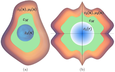
Figure 1: Sketch of the system under study. In the configuration on the right the sum of the Casimir-Lifshitz forces on each object equals zero. In both cases the force acting on the surface of the sphere due to the interaction with the magnetodielectric cavity can be considered. Between both objects there is another frequency-dependent, but homogeneous, dielectric.

Throughout this paper we will use the natural units $\hslash=c=\varepsilon_{0}=\mu_{0}=1$, neglecting fluctuations due to nonelectromagnetic oscillations when the medium is different from vacuum, which are usually small dzyaloshinskii1961general .

We assume that the coupling of the electromagnetic field to matter can be described by continuous permittivity $\varepsilon$ and permeability ${\mu}$ functions. For a homogeneous medium characterized by $\varepsilon_{M}$ and $\mu_{M}$, Maxwell curl equations, after Fourier transform in time, can be rearranged to give a stationary vector Schrödinger-like equation newton2013scattering

$$\left[\boldsymbol{\nabla}\times\boldsymbol{\nabla}+\mathbb{V}(\omega,\mathbf{x})\right]\textbf{E}(\omega,\mathbf{x})=k^{2}\textbf{E}(\omega,\mathbf{x}),$$ (2)

where $k\equiv\sqrt{\varepsilon_{M}}\omega$ and the potential operator $\mathbb{V}(\omega,\mathbf{x})$ is

$$\mathbb{I}{\omega^{2}}\left[\varepsilon_{M}(\omega)-\varepsilon(\omega,\textbf{x})\right]+\boldsymbol{\nabla}\times\left[\frac{1}{\mu(\omega,\textbf{x})}-\frac{1}{\mu_{M}(\omega)}\right]\boldsymbol{\nabla}\times.$$

Since the magnetic response of ordinary materials is typically close to one, we will focus on nonmagnetic bodies. However, we shall see that in some cases the introduction of nontrivial permeabilities poses no additional difficulties, especially for the cavity. In any case, we deal with two nonoverlapping bodies. Specifically, if ${\mu(\omega,\textbf{x})}={\mu_{M}(\omega)}=1$ we have

$$\mathbb{V}_{i}(\omega,\textbf{x})=\mathbb{I}{V}_{i}(\omega,\textbf{x})=\mathbb{I}\omega^{2}\left[\varepsilon_{M}(\omega)-\varepsilon_{i}(\omega,\textbf{x})\right],$$ (3)

being $\text{supp}\,V_{1}\cap\,\text{supp}\,V_{2}=\emptyset$. Here supp stands for the spatial support of the function. Consequently, the Casimir interaction energy between the two objects is encapsulated in the so-called TGTG formula kenneth2008casimir ; rahi2009scattering

$$E_{\text{int}}=\frac{1}{2\pi}\int_{0}^{\infty}d\kappa\,\text{Tr}\log(\mathbb{I}-{\mathbb{T}_{1}}\mathbb{G}^{M}_{12}\mathbb{{T}}_{2}\mathbb{G}^{M}_{21}).$$ (4)

As usual, we will carry out the integration over imaginary frequencies $\omega=i\kappa$. In this sense, we denote by $\varepsilon(i\kappa)$ the analytic continuation of the permittivity to the imaginary frequency axis, which from Kramers-Kronig causality conditions satisfies $\varepsilon(i\kappa)\geq 1$ bordag2009advances . The properties of each body are encoded in the Lippmann-Schwinger $\mathbb{T}$ operator $\mathbb{T}_{i}:\mathcal{H}_{i}\to\mathcal{H}_{i}$, being $\mathcal{H}_{i}\equiv L^{2}(\text{supp}\,\mathbb{V}_{i})^{3}$ hanson2013operator . Furthermore, the relative position between both objects enters through the operator $\mathbb{G}^{M}_{ij}\equiv\mathbb{P}_{i}\mathbb{G}^{M}\mathbb{P}_{j}:\mathcal{H}_{j}\to\mathcal{H}_{i},$ being $\mathbb{G}^{M}$ the propagator across the medium and $\mathbb{P}_{i}$ the projection operator onto the Hilbert space $\mathcal{H}_{i}$. The electric Green’s dyadics fulfill

$$\left[\boldsymbol{\nabla}\times\boldsymbol{\nabla}\times+\varepsilon_{M}(i\kappa){\kappa^{2}}\right]\mathbb{G}^{M}(i\kappa,\mathbf{x},\mathbf{x}^{\prime})=~{}\mathbb{I}\delta(\mathbf{x}~{}-~{}\mathbf{x}^{\prime}),$$

which are related to the vacuum functions by

$$\mathbb{G}^{0}(i\sqrt{\varepsilon_{M}}\kappa,\mathbf{x},\mathbf{x}^{\prime})=\mathbb{G}^{M}(i\kappa,\mathbf{x},\mathbf{x}^{\prime}).$$

Writing $\mathbb{G}^{M}$ in terms of the Green’s function for the scalar Helmholtz equation, it can be proved that $\langle\textbf{E},\mathbb{G}^{M}\textbf{E}\rangle\geq~{}0$ for all the vectors E hanson2013operator ; rahi2010constraints . Namely, $\mathbb{G}^{M}$ is a nonnegative operator $\mathbb{G}^{M}\geq~{}0$. In addition, these functions are related to the $\mathbb{T}_{i}$ operators by $\mathbb{T}_{i}=\mathbb{V}_{i}/({\mathbb{I}+\mathbb{G}^{M}\mathbb{V}_{i}}),$ where the Lippmann-Schwinger equation of electromagnetic scattering is formally written as $\textbf{E}=\textbf{E}_{0}-\mathbb{G}^{M}\mathbb{T}_{i}\textbf{E}_{0}.$ We will not analyze convergence issues or the self-adjointness of the presented operators (for those see hanson2013operator ), assuming that the appropriate conditions are fulfilled in realistic systems rahi2010constraints .

Since the two bodies are separated from each other, we can expand the Green’s functions in terms of free solutions of Eq. (2). In spherical coordinates there is a regular solution at the origin $\textbf{E}_{a}^{\text{rg}}(\omega,\textbf{x})$, whose radial part is determined by the spherical Bessel function $j_{\ell}(\omega r)$, and an outgoing (incoming) solution $\textbf{E}_{a}^{\text{out}}(\omega,\textbf{x})$ [$\textbf{E}_{a}^{\text{in}}(\omega,\textbf{x})$], whose radial part is determined by the spherical Hankel function of the first (second) kind $h^{(1)}_{\ell}(\omega r)$ [$h^{(2)}_{\ell}(\omega r)$] sun2019invariant . The subscript of these transverse solutions stands for the angular momentum values $\{\ell,{m}\}$ and polarizations. Based on the appropriate representation of $\mathbb{G}^{M}_{ij}$ when the two bodies lie entirely outside each other, the operator ${\mathbb{T}_{1}}\mathbb{G}^{M}_{12}\mathbb{{T}}_{2}\mathbb{G}^{M}_{21}$ in Eq. (4) can be expanded as

$$\langle\textbf{E}_{j}^{\text{rg}},{\mathbb{T}_{1}}\textbf{E}_{a}^{\text{rg}}\rangle\langle\textbf{E}_{a}^{\text{rg}},\mathbb{G}^{M}_{12}\textbf{E}_{b}^{\text{rg}}\rangle\langle\textbf{E}_{b}^{\text{rg}},\mathbb{{T}}_{2}\textbf{E}_{c}^{\text{rg}}\rangle\langle\textbf{E}_{c}^{\text{rg}},\mathbb{G}^{M}_{21}\textbf{E}_{k}^{\text{rg}}\rangle,$$ (5)

where a sum over $a,b,c$ is assumed. In this case $\langle\textbf{E}_{j}^{\text{rg}},{\mathbb{T}_{i}}\textbf{E}_{k}^{\text{rg}}\rangle$ encodes the usual scattering amplitude related to a process in which a regular wave interacts with an object and scatters outward newton2013scattering . The sum changes to

$$\langle\textbf{E}_{j}^{\text{rg}},{\mathbb{T}_{1}}\textbf{E}_{a}^{\text{rg}}\rangle\langle\textbf{E}_{a}^{\text{rg}},\mathbb{G}^{M}_{12}\textbf{E}_{b}^{\text{in}}\rangle\langle\textbf{E}_{b}^{\text{in}},\mathbb{{T}}_{2}\textbf{E}_{c}^{\text{out}}\rangle\langle\textbf{E}_{c}^{\text{out}},\mathbb{G}^{M}_{21}\textbf{E}_{k}^{\text{rg}}\rangle$$ (6)

for interior configurations, where one body is inside the other. In this less common version of the $TGTG$ representation, the usual scattering amplitude arises for the first body and $\langle\textbf{E}_{b}^{\text{in}},\mathbb{{T}}_{2}\textbf{E}_{c}^{\text{out}}\rangle$ for the cavity. The latter is associated with a scattering experiment in which the source and the detector are inside the cavity rahi2009scattering . In this regard, expansion (6) offers a schematic description of the travel of the wave between both bodies: a regular wave reaches the first body, part of the wave is reflected as an outgoing wave heading towards the cavity, where is partially scattered as an incoming wave, contributing to form the regular wave which reaches the first body and the process is repeated. This iteration clearly reveals the nonadditive character of fluctuation-induced forces. In line with this, an alternative proof of the $TGTG$ formula for symmetric bodies based on the mode summation approach is given in teo2012mode . Although the $TGTG$ representation in terms of operators is formally the same, we want to emphasize that the suitable Green’s function expansions depend on the configuration.

In order to determine the sign of the Casimir energy we assume that the sign $s_{i}$ of the potential $V_{i}$ in Eq. (3) is constant over the whole body, being

$$s_{i}=\pm 1\ \ \text{if}\ \ \varepsilon_{i}(i\kappa,\textbf{x})\gtrless\varepsilon_{M}(i\kappa),\ \ \forall\textbf{x}\in\text{supp}\,V_{i}.$$ (7)

In this case $\mathbb{T}_{i}(i\kappa)$ is real and symmetric and can be written in the form $\mathbb{T}_{i}=s_{i}\sqrt{s_{i}\mathbb{T}_{i}}\sqrt{s_{i}\mathbb{T}_{i}},$ where $\sqrt{s_{i}\mathbb{T}_{i}}$ is the square root of the positive operator $s_{i}\mathbb{T}_{i}$ rahi2010constraints . We shall see that our analysis applies to each fixed frequency so Eq. (7) should hold for all of them. However, we can simply assume constant sign over the frequencies contributing most to the energy dzyaloshinskii1961general ; munday2009measured . Accordingly, the interaction energy can be rewritten as

$$E_{\text{int}}=\frac{1}{2\pi}\int_{0}^{\infty}d\kappa\,\text{Tr}\log(\mathbb{I}-s\,\mathbb{M}),$$ (8)

where we have defined $\mathbb{M}\equiv\sqrt{s_{2}\mathbb{T}_{2}}\mathbb{G}^{M}_{21}{s_{1}\mathbb{T}_{1}}\mathbb{G}^{M}_{12}\sqrt{s_{2}\mathbb{T}_{2}}$ and $s\equiv s_{1}s_{2}$. The representations (4) and (8) are equivalent since

$$\text{Tr}\log(\mathbb{I}-s\,\mathbb{M})=\text{Tr}\log(\mathbb{I}-{\mathbb{T}_{1}}\mathbb{G}^{M}_{12}\mathbb{{T}}_{2}\mathbb{G}^{M}_{21}).$$

This follows from $\text{Tr}\log(\mathbb{I}-s\,\mathbb{M})=\log\det(\mathbb{I}-s\,\mathbb{M})$ and the determinant identity $\det(\mathbb{I}-\mathbb{A}\mathbb{B})=\det(\mathbb{I}-\mathbb{B}\mathbb{A})$, where $\mathbb{A}\mathbb{B}=s\,\mathbb{M}$ and $\mathbb{B}\mathbb{A}={\mathbb{T}_{1}}\mathbb{G}^{M}_{12}\mathbb{{T}}_{2}\mathbb{G}^{M}_{21}$ simon1977notes . In addition, using $(\mathbb{G}^{M}_{ij})^{\dagger}=\mathbb{G}^{M}_{ji}$, we rewrite this new operator as

$$\mathbb{M}=(\sqrt{s_{1}\mathbb{T}_{1}}\mathbb{G}^{M}_{12}\sqrt{s_{2}\mathbb{T}_{2}})^{\dagger}\sqrt{s_{1}\mathbb{T}_{1}}\mathbb{G}^{M}_{12}\sqrt{s_{2}\mathbb{T}_{2}},$$ (9)

proving that it is nonnegative. We will frequently make use of this standard reasoning, which follows from the definition of the adjoint:

$$\langle\textbf{E},{\mathbb{C}^{\dagger}}\mathbb{C}\textbf{E}\rangle=\langle{\mathbb{C}}\textbf{E},\mathbb{C}\textbf{E}\rangle=\|\mathbb{C}\textbf{E}\|^{2}\geq 0.$$ (10)

The eigenvalues of $\mathbb{M}$, besides being nonnegative, belong to $[0,1)$. This has been proved for the operator $\mathbb{T}_{1}\mathbb{G}^{0}_{12}\mathbb{{T}}_{2}\mathbb{G}^{0}_{21}$ when the intermediate medium is vacuum, $\mathbb{T}_{i}>0$, thus obtaining $E_{\textup{int}}~{}\leq~{}0$ kenneth2008casimir . In our case, the same derivation holds replacing $\mathbb{T}_{i}$ and $\mathbb{G}^{0}$ by $s_{i}\mathbb{{T}}_{i}>0$ and $\mathbb{G}^{M}$, noting that the nonzero eigenvalues of $s\mathbb{A}\mathbb{B}=\mathbb{M}$ and $s\mathbb{B}\mathbb{A}=s{\mathbb{T}_{1}}\mathbb{G}^{M}_{12}\mathbb{{T}}_{2}\mathbb{G}^{M}_{21}$ are the same. It is then clear that we can also obtain $E_{\textup{int}}~{}>~{}0$. First, using Lidskii’s theorem the trace in Eq. (8) can be expressed as

$$\text{Tr}\log(\mathbb{I}-s\,\mathbb{M})=\sum_{\alpha}\log(1-s\lambda_{\alpha}),\quad\mathbb{M}\textbf{E}_{\alpha}=\lambda_{\alpha}\textbf{E}_{\alpha}.$$

Consequently, if $\lambda_{\alpha}\neq 0$ we have $s=-\textup{sgn}\log(1-s\lambda_{\alpha})$ and $\textup{sgn}\,E_{\textup{int}}=-s$. The latter can be written in terms of the permittivities as

$$\textup{sgn}\,E_{\textup{int}}=-s=-\textup{sgn}\left[(\varepsilon_{1}-\varepsilon_{M}\right)(\varepsilon_{2}-\varepsilon_{M})].$$ (11)

For magnetodielectric objects characterized by $\varepsilon_{i}$ and $\mu_{i}$, the relation $\textup{sgn}\,E_{\textup{int}}=-s$ remains valid as long as the sign of the differential operator $\mathbb{V}_{i}(i\kappa,\mathbf{x})$ in Eq. (2) is well-defined. The latter is determined by Eq. (7) if we include an additional condition:

$$s_{i}=\pm 1\quad\text{if}\ \varepsilon_{i}(i\kappa,\textbf{x})\gtrless\varepsilon_{M}(i\kappa)\ \text{and}\ \mu_{i}(i\kappa,\textbf{x})~{}\lesseqgtr~{}\mu_{M}(i\kappa),$$

for the whole body rahi2009scattering . It is also worth emphasizing that the result on the sign of the energy (11) is valid for two arbitrary bodies, even when they lie outside each other.

3 Interaction pressure

The Casimir-Lifshitz interaction pressure acting on the surface of the sphere can be obtained from the representation of the energy given in Eq. (8). To define this pressure we do not need to include elastic deformations, we simply make use of the principle of virtual work. Accordingly, the mean value of the pressure due to a virtual variation of the radius of the sphere $r_{1}$ satisfies barton2004casimir ; li2019casimir

$$\langle p_{\text{int}}\rangle\equiv\dfrac{1}{4\pi}\int_{S^{2}}d\Omega\,p_{\text{int}}(r_{1},\Omega)=-\dfrac{1}{4\pi r_{1}^{2}}\frac{\partial E_{\text{int}}}{\partial r_{1}}.$$ (12)

In particular, for a spherically symmetric system the pressure is constant $\langle p_{\text{int}}\rangle=p_{\text{int}}(r_{1}).$ In order to evaluate the sign of $\partial_{r_{1}}E_{\text{int}}$ we employ the variable phase approach of electromagnetic scattering johnson1988invariant . This method is progressively reaching some importance in Casimir physics since it enables to compute efficiently $\mathbb{T}_{i}$ for nonsymmetric objects forrow2012variable . Specifically, in order to prove $\partial_{r_{1}}(s_{1}\mathbb{T}_{1})>0$ we make use of the quantum mechanical Calogero equation calogero1967variable generalized to electromagnetic scattering by arbitrarily shaped objects johnson1988invariant ; sun2019invariant

$$\frac{\partial{T}_{1}}{\partial{r_{1}}}=-ik({J}_{1}+{H}_{1}{T}_{1})^{T}{U}_{1}({J}_{1}+{H}_{1}{T}_{1}).$$ (13)

The superscript $T$ denotes the transpose operation and ${T}_{1}$ is the $\mathbb{T}_{1}$ operator in the spherical wave basis, i.e., $({T}_{1})_{{a}{b}}$ stands for $\langle\textbf{E}_{a}^{\text{rg}},{\mathbb{T}_{1}}\textbf{E}_{b}^{\text{rg}}\rangle$ of expansion (5) in terms of the complete set of regular solutions. Furthermore, the potential $V_{1}$ defined in Eq. (3) enters through

$$\langle\textbf{E}_{\ell{m}}^{\text{rg}},{U}_{1}\textbf{E}_{\ell^{\prime}{m}^{\prime}}^{\text{rg}}\rangle=r^{2}\int_{S^{2}}d\Omega\,{Y}^{\dagger}_{\ell{m}}V_{1}(\omega,\textbf{x}){D}(\omega,\textbf{x}){Y}_{\ell^{\prime}{m}^{\prime}},$$

being the matrix ${Y}_{\ell{m}}$ composed of vector spherical harmonics and ${D}(\omega,\textbf{x})=\text{diag}(\varepsilon_{M}(\omega)/\varepsilon_{1}(\omega,\textbf{x}),1,1)$ sun2019invariant . For imaginary frequencies we have defined the two real matrices ${J}_{1}$ and ${H}_{1}$

$$\langle\textbf{E}_{\ell{m}}^{\text{rg}},{J}_{1}(i\xi)\textbf{E}_{\ell^{\prime}{m^{\prime}}}^{\text{rg}}\rangle=\frac{1}{r_{1}}\left(\begin{array}[]{cc}i_{\ell}(\xi r_{1})&0\\ 0&\partial_{r_{1}}i_{\ell}(\xi r_{1})\\ 0&\dfrac{i_{\ell}(\xi r_{1})}{r_{1}}\\ \end{array}\right)\delta_{\ell\ell^{\prime}}\delta_{{m}{m}^{\prime}},$$

$$\langle\textbf{E}_{\ell{m}}^{\text{rg}},{H}_{1}(i\xi)\textbf{E}_{\ell^{\prime}{m^{\prime}}}^{\text{rg}}\rangle=\frac{1}{r_{1}}\left(\begin{array}[]{cc}k_{\ell}(\xi r_{1})&0\\ 0&\partial_{r_{1}}k_{\ell}(\xi r_{1})\\ 0&\dfrac{k_{\ell}(\xi r_{1})}{r_{1}}\\ \end{array}\right)\delta_{\ell\ell^{\prime}}\delta_{{m}{m}^{\prime}},$$

in terms of $\xi\equiv{\kappa}{\sqrt{\varepsilon_{M}}}$ and the modified Bessel functions

$$i_{\ell}(z)\equiv\sqrt{{\pi}/2z}\,I_{\ell+{1}/{2}}(z),\quad k_{\ell}(z)\equiv\sqrt{2/\pi z}\,K_{\ell+{1}/{2}}(z).$$

To reach this expressions we have used the same expansion of the background Green’s functions as in johnson1988invariant ; sun2019invariant

$$\mathbb{G}^{M}({\bf x},{\bf x}^{\prime})=\xi\sum_{a}\left\{\begin{array}[]{cc}{\bf E}_{a}^{\rm out}({\bf x})\otimes{\bf E}_{a}^{{\rm reg*}}({\bf x}^{\prime})&\ {\rm if}\ \ r>r^{\prime},\\[2.15277pt] {\bf E}_{a}^{{\rm reg}}({\bf x})\otimes{\bf E}_{a}^{{\rm out*}}({\bf x}^{\prime})&\ {\rm if}\ \ r<r^{\prime}.\end{array}\right.$$

Each mode of the electric field is determined by the transverse electric (TE) and magnetic (TM) vectors

$${\mathbf{M}}^{\text{rg}}_{\ell m}(i\xi,\mathbf{x}) = \frac{1}{\sqrt{\ell(\ell+1)}}\ \boldsymbol{\nabla}\times\phi^{\text{rg}}_{\ell m}(i\xi,\mathbf{x})\,\mathbf{x},$$

$$\mathbf{M}^{\text{out}}_{\ell m}(i\xi,\mathbf{x}) = \frac{1}{\sqrt{\ell(\ell+1)}}\ \boldsymbol{\nabla}\times\phi^{\text{out}}_{\ell m}(i\xi,\mathbf{x})\,\mathbf{x},$$

$$\mathbf{N}^{\text{rg}}_{\ell m}(i\xi,\mathbf{x}) = \frac{1}{\xi\sqrt{\ell(\ell+1)}}\ \boldsymbol{\nabla}\times\boldsymbol{\nabla}\times\phi^{\text{rg}}_{\ell m}(i\xi,\mathbf{x})\,\mathbf{x},$$

$$\mathbf{N}^{\text{out}}_{\ell m}(i\xi,\mathbf{x}) = \frac{1}{\xi\sqrt{\ell(\ell+1)}}\ \boldsymbol{\nabla}\times\boldsymbol{\nabla}\times\phi^{\text{out}}_{\ell m}(i\xi,\mathbf{x})\,\mathbf{x},$$

which can be expressed in terms of the scalar Helmholtz equation solutions rahi2009scattering

$$\phi^{\text{rg}}_{\ell m}(i\xi,\mathbf{x})=i_{l}(\xi r)Y^{m}_{\ell}(\Omega),\quad\phi^{\text{out}}_{\ell m}(i\xi,\mathbf{x})=k_{l}(\xi r)Y^{m}_{\ell}(\Omega).$$

Nevertheless, the relevant fact is the structure of the right-hand side of Eq. (13), which naturally leads to the positivity of $s_{1}\partial_{r_{1}}{T}_{1}$. Along the imaginary frequency axis ${T}_{1}$ is real and symmetric, consequently, using Eq. (10), $s_{1}\partial_{r_{1}}{T}_{1}$ is positive if $s_{1}{U}_{1}$ is, and, for the same reason, the latter is positive if $s_{1}V_{1}(i\kappa,\textbf{x})>0$, which holds trivially assuming (7).

As a consistency test, we prove by explicit calculation that $s_{1}\partial_{r_{1}}{\mathbb{T}_{1}}$ is positive for a spherically symmetric object [Fig. 1(b)]. In this case we can make use of the standard Lorenz-Mie theory johnson1999exact . The problem is completely decoupled for the angular momentum values and the two polarizations. Indeed, electromagnetic scattering reduces to two independent scalar problems, one for each polarization johnson1999exact . For instance, the two radial potentials for a homogeneous sphere are

$$V_{1}^{\textup{TE}}(\omega)=V_{1}^{\textup{TM}}(\omega)=\omega^{2}\left[\varepsilon_{M}(\omega)-\varepsilon_{1}(\omega)\right],$$

being $V_{1}^{\textup{TE}}(\omega,r)=\omega^{2}\left[\varepsilon_{M}(\omega)-\varepsilon_{1}(\omega,r)\right]$ valid for any spherically symmetric object toni2014advances . Consequently, we can write

$$\langle\textbf{E}^{\text{rg}}_{\ell{m}},\mathbb{T}\,\textbf{E}^{\text{rg}}_{\ell^{\prime}{m}^{\prime}}\rangle=\left(\begin{array}[]{cc}{T}^{\textup{TE}}_{\ell}&0\\ 0&{T}^{\textup{TM}}_{\ell}\\ \end{array}\right)\delta_{\ell\ell^{\prime}}\delta_{{m}{m}^{\prime}},$$ (16)

where the subscript in $\mathbb{T}_{1}$ and the $i\kappa$ dependence have been omitted for simplicity. Rotating to imaginary frequencies the derivatives of the Lorenz-Mie coefficients rahi2009scattering ; johnson1999exact , we obtain the following first-order nonlinear differential equations:

$$s_{1}\partial_{r_{1}}{T}^{\textup{TE}}_{\ell} = s_{1}\left({\varepsilon_{1}({r_{1}})}-{\varepsilon_{M}}\right)\frac{a_{1}^{2}\kappa{r_{1}}}{2\pi{\varepsilon_{M}}},$$

$$s_{1}\partial_{r_{1}}{T}^{\textup{TM}}_{\ell} = s_{1}\left({\varepsilon_{1}({r_{1}})}-\varepsilon_{M}\right)\frac{a_{2}^{2}\ell(\ell+1)+a_{3}^{2}{\varepsilon_{1}({r_{1}})}/{\varepsilon_{M}}}{2\pi\kappa{r_{1}}\,{\varepsilon_{1}({r_{1}})}}.$$

Both derivatives are positive since the three parameters $a_{i}$ are real:

$$a_{1} = -2{T}^{\textup{TE}}_{\ell{m}}\kappa K_{\ell+{1}/{2}}(\kappa{r_{1}})+\pi I_{\ell+{1}/{2}}(\kappa{r_{1}}),$$

$$a_{2} = \pi I_{\ell+{1}/{2}}(\kappa{r_{1}})+2{T}^{\textup{TM}}_{\ell{m}}\kappa K_{\ell+{1}/{2}}(\kappa{r_{1}}),$$

$$a_{3} = 2\kappa{T}^{\textup{TM}}_{\ell{m}}\left[(\ell+1)K_{\ell+{1}/{2}}(\kappa{r_{1}})-\kappa{r_{1}}K_{\ell+{3}/{2}}(\kappa{r_{1}})\right]$$

$$+ \pi\kappa{r_{1}}I_{\ell+{3}/{2}}(\kappa{r_{1}})+\pi(\ell+1)I_{\ell+{1}/{2}}(\kappa{r_{1}}).$$

Having proved $\partial_{r_{1}}({s_{1}\mathbb{T}_{1}})>0$, we can straightforwardly find the sign of $\langle p_{\textup{int}}\rangle$. We simply note that only $\mathbb{T}_{1}$ depends on $r_{1}$ in $\mathbb{M}$, i.e., we can write

$$\partial_{r_{1}}\mathbb{M}=\left(\mathbb{G}^{M}_{12}\sqrt{s_{2}\mathbb{T}_{2}}\right)^{\dagger}\partial_{r_{1}}({s_{1}\mathbb{T}_{1}})\left(\mathbb{G}^{M}_{12}\sqrt{s_{2}\mathbb{T}_{2}}\right)>0.$$

As before, the positivity is proved using Eq. (10). Applying the Hellmann-Feynman theorem to the eigenvalues of $\mathbb{M}$, we obtain $\partial_{r_{1}}\lambda_{\alpha}>0$ feynman1939forces . With this, $\textup{sgn}\,\partial_{r_{1}}\log(1-s\lambda_{\alpha})=-s$. Finally, from Eq. (8) and Lidskii’s theorem we obtain $\text{sgn}\,\partial_{r_{1}}E_{\text{int}}=-s$, which can be written in terms of the pressure with Eq. (12)

$$\textup{sgn}\langle p_{\textup{int}}\rangle=s=\textup{sgn}\left[(\varepsilon_{1}-\varepsilon_{M}\right)(\varepsilon_{2}-\varepsilon_{M})].$$ (17)

This is the main result of our work. Since we have considered permittivity functions $\varepsilon(i\kappa,\textbf{x})$ such that the sign of $\varepsilon_{i}(i\kappa,\textbf{x})-\varepsilon_{M}(i\kappa)$ is independent of $\kappa$ and x, we have written $\textup{sgn}(\varepsilon_{i}-\varepsilon_{M})=\textup{sgn}[\varepsilon_{i}(i\kappa,\textbf{x})-\varepsilon_{M}(i\kappa)]$.

We now compare this result with particular configurations previously studied in the literature. First, for two concentric spherical shells satisfying perfectly conducting boundary conditions a positive pressure is obtained using the zeta function regularization method teo2010casimir . This is consistent with Eq. (17) since these idealized conditions arise in the limit of large permittivities. This positive pressure is also found in the experimental setup suggested in brevik2005casimir , where the same boundary conditions are considered using Green’s functions. Secondly, based on a quantum statistical approach, the pressure acting on the surface of a homogeneous spherical cavity sharing center with a sphere of the same material is computed in hoye2001casimir . The medium between both bodies is vacuum, but as the authors mention, their results can be easily generalized considering the same geometry with three different permittivities $\{\varepsilon_{1},\varepsilon_{2},\varepsilon_{M}\}$. In this case, the coefficient $A_{\ell}$ defined in hoye2001casimir , fulfilling ${\textup{sgn}\,A_{\ell}=\textup{sgn}\,\langle p_{\textup{int}}\rangle}$, changes to

$$A_{\ell}=\frac{\left[\varepsilon_{1}(i\kappa)-\varepsilon_{M}(i\kappa)\right]\left[\varepsilon_{2}(i\kappa)-\varepsilon_{M}(i\kappa)\right]\ell(\ell+1)}{\left[\ell\varepsilon_{1}(i\kappa)+\varepsilon_{M}(i\kappa)(\ell+1)\right]\left[\ell\varepsilon_{M}(i\kappa)+\varepsilon_{2}(i\kappa)(\ell+1)\right]},$$

so the sign of pressure acting on the surface of the sphere satisfies Eq. (17).

4 Repulsive pressure and DLP configuration

In current experimental setups, such as those mentioned in Sec. 1, the interaction force between at least two bodies is measured garrett2018measurement . This quantity arises from the dependence of the Casimir energy on the distance between bodies, which excludes self-energy contributions. Indeed, it is not clear if the latter are observationally well-defined hoye2001casimir . In the preceding section we have studied the pressure due to the interaction term of the energy, which might also be the relevant one in this context hoye2001casimir ; brevik2005casimir . Indeed, we will recover the DLP result for the interaction force from a limiting case of $\textup{sgn}\langle p_{\textup{int}}\rangle$ in Eq. (17). However, there is no straightforward way to measure this pressure in general geometries and effects of different origin, such as hydrodynamic forces in liquid dielectrics, should be taken into account. In any case, we will determine the sign of the total pressure for certain configurations described by permittivity $\varepsilon$ and permeability ${\mu}$ functions. The Casimir energy is written as

$$E_{C}=E_{1}+E_{2}+E_{\text{int}}.$$ (18)

As we have described, the Casimir force between bodies with disjoint support is free of divergences. This is based on the local nature of the heat kernel coefficients, which determine the divergent part of the vacuum energy bordag2009advances . However, the ultraviolet divergences contained in the self-energies can not always be satisfactorily removed. For homogeneous magnetodielectric spheres, although several regularization procedures have been proposed bordag2009advances ; milton2020self , to our knowledge the Casimir energy can only be defined in two special cases: when the speed of light is identical both inside and outside the sphere and in the dilute approximation milton2001casimir . In the latter, when the surrounding medium is vacuum, the renormalized self-energy is

$$E_{1}^{\text{ren}}=\dfrac{23}{1536\pi r_{1}}\left(\varepsilon_{1}-1\right)^{2}+O\left(\varepsilon_{1}-1\right)^{3}.$$ (19)

In addition, the actual computation of the interaction energy could be simplified. Assuming $\varepsilon_{i}\simeq 1$, we can expand $\log(\mathbb{I}-s\,\mathbb{M})$ in Eq. (8) as

$$\text{Tr}\log(\mathbb{I}-s\,\mathbb{M})=-\sum_{j=1}^{\infty}\frac{\text{Tr}(\mathbb{I}-s\,\mathbb{M})^{j}}{j}$$ (20)

and take only the leading terms. Also, the operator $\mathbb{T}_{i}=\mathbb{V}_{i}/({\mathbb{I}+\mathbb{G}^{M}\mathbb{V}_{i}})$ can be expanded in powers of $\varepsilon_{i}-1$ kenneth2008casimir .

Using the principle of virtual work, noting that the self-energy of the cavity $E_{2}$ is independent of $r_{1}$, we define the total pressure on the sphere as

$$\langle p\rangle\equiv-\dfrac{1}{4\pi r_{1}^{2}}\left(\frac{\partial E^{\text{ren}}_{1}}{\partial r_{1}}+\frac{\partial E_{\text{int}}}{\partial r_{1}}\right).$$ (21)

We then consider the configuration shown in Fig. 1(a) with dielectric response functions such that $\varepsilon_{1}$ is close to one and $\varepsilon_{2}(i\kappa,\textbf{x})>\varepsilon_{1}$ for the whole cavity. From the renormalized energy (19) it is clear that the self-pressure is repulsive, i.e., it tends to expand the sphere. In addition, from Eq. (17), we know that $\varepsilon_{2}>\varepsilon_{1}>\varepsilon_{M}=1$ also results in a positive interaction pressure. Consequently, we obtain $\langle p\rangle>0$.

It should be mentioned that the tendency to expand the sphere would be described as an attractive interaction force as outlined in Sec. 1. We can see it explicitly recovering the DLP result from Eq. (17). Firstly, the planar geometry is reached if we assume a spherical cavity with inner radius $r_{2}$ and take the limits $r_{i}\to\infty$, being $d\equiv r_{2}-r_{1}$ constant cavero2020casimir . The interaction force per unit area $F_{\text{int}}$ may be defined analogously to the pressure in Eq. (12), using now variations of the distance between bodies. Noting that $\partial_{r_{1}}E_{\text{int}}=-\partial_{d}E_{\text{int}}$, from Eq. (17) we finally obtain the DLP result (1)

$$\textup{sgn}\,F_{\textup{int}}=-\textup{sgn}\left[(\varepsilon_{1}-\varepsilon_{M}\right)(\varepsilon_{2}-\varepsilon_{M})].$$ (22)

As we have mentioned in Sec. 1, this gives rise to repulsive forces if $\varepsilon_{2}>\varepsilon_{M}>\varepsilon_{1}$, and to attractive ones if $\varepsilon_{2}>\varepsilon_{1}>~{}\varepsilon_{M}$. Both cases have been confirmed experimentally munday2009measured . Furthermore, we have proved that the DLP result can be extended to inhomogeneous slabs as long as Eq. (7) holds.

5 Extensions and concluding remarks

We complete this work presenting some remarks on the main result. In particular, we generalize the configuration considered in Sec. 3 to magnetodielectric cavities and systems at thermal equilibrium.
(1) Magnetodielectric cavity. The electromagnetic Calogero equation (13) requires the homogeneous background and the scattering object to be nonmagnetic. However, in order to determine the sign of $\langle p_{\textup{int}}\rangle$ we have only assumed a well-defined sign of $\mathbb{T}_{2}(i\kappa)$, i.e., $\langle p_{\textup{int}}\rangle=s_{1}s_{2}$. Therefore, we can consider a cavity described by functions $\varepsilon_{2}$ and $\mu_{2}$, such that

$$s_{2}=\pm 1\quad\text{if}\ \varepsilon_{2}(i\kappa,\textbf{x})\gtrless\varepsilon_{M}(i\kappa)\ \text{and}\ \mu_{2}(i\kappa,\textbf{x})~{}\lesseqgtr~{}\mu_{M}(i\kappa),$$

for the whole body rahi2009scattering . In addition, since $E_{1}$ is independent of the second object, the total pressure defined in Eq. (21) is positive if $s_{2}=1$ and $\varepsilon_{2}(\omega,\textbf{x})>\varepsilon_{1}$.
(2) Finite $T$. The extension of results (11) and (17) to quantum systems at thermal equilibrium follows from the Matsubara formulation. The free energy $F_{\text{int}}$ satisfies milton2001casimir

$$\langle p_{\text{int}}\rangle=-\frac{1}{4\pi r_{1}^{2}}\,\frac{\partial F_{\text{int}}}{\partial r_{1}},$$ (23)

and we can compute it replacing the integral in $E_{\textup{int}}$ by a sum over the Matsubara frequencies $\kappa_{n}~{}=~{}2\pi k_{\text{B}}{n}T$, where the zero mode is weighted by $1/2$ and the temperature enters as a multiplicative factor bordag2009advances :

$$F_{\text{int}}=k_{B}T\sum_{n=0}^{\infty}{}^{\prime}\ \text{Tr}\log\left[\mathbb{I}-s\,\mathbb{M}(i\kappa_{n})\right].$$ (24)

With this, results (11) and (17) can be reproduced with minor changes. We simply notice that we have treated each frequency separately and that $\partial_{r_{1}}({s_{1}\mathbb{T}_{1}})~{}>~{}0$, which refers only to electromagnetic scattering, also applies. In the dilute approximation, the free energy of the sphere at low temperature is milton2001casimir

$$F_{1}^{\text{ren}}\simeq\left(\varepsilon_{1}-1\right)^{2}\left[\dfrac{23}{1536\pi r_{1}}+\dfrac{7}{270}(\pi r_{1})^{3}T^{4}\right],$$

where the additional term counteracts the zero temperature repulsion. Nevertheless, if $T$ is small enough we still obtain a total positive pressure.
(3) Energy, force and stable levitation. The Casimir force can switch from attractive to repulsive when the sign of the energy changes. This has been proved in planar geometries for a scalar field satisfying a four parameter family of boundary conditions at the plates asorey2013attractive and for inhomogeneous dielectrics slabs, being the the sign of the force given by Eq. (22) and the sign of the energy by Eq. (11). The same holds for mirror symmetric objects: the force between them is attractive being the interaction energy always negative kenneth2006opposites . In addition, the condition determining unstable levitation based on Casimir-Lifshitz forces is also governed by the sign of the energy rahi2010constraints . In particular, $s>0$ implies unstable levitation, being $s=-\text{sgn}\,E_{\text{int}}$ as we have proved. Similarly, in the present case,

$$\textup{sgn}\,E_{\textup{int}}=-\textup{sgn}\,\langle p_{\text{int}}\rangle.$$

Indeed, stable levitation is possible if, and only if, the pressure is negative. However, there are nontrivial configurations where attractive and repulsive forces are found for constant values of $\text{sgn}\,E_{\textup{int}}$ levin2010casimir ; abrantes2018repulsive .
(4) Exterior configuration. For both expansions of the operator ${\mathbb{T}_{1}}\mathbb{G}^{M}_{12}\mathbb{{T}}_{2}\mathbb{G}^{M}_{21}$ in an exterior or a cavity configuration, (5) and (6), the scattering amplitude $\langle\textbf{E}_{i}^{\text{rg}},{\mathbb{T}_{1}}\textbf{E}_{a}^{\text{rg}}\rangle$ characterizes the first body. As we have already discussed, the scattering amplitudes are only different for the second body. Then, the result on the sign of the pressure holds for a exterior configuration, being the net force acting on the sphere in general nonzero.

Conclusions

We are able to determine the tendency of the interaction pressure to expand or contract the sphere. The result does not depend either on the geometry of the cavity or on the matter distribution inside the sphere, as long as the assumption (7) holds. Since the proof applies to each frequency independently, the extension to systems at thermal equilibrium is almost immediate. We find that the sign of the pressure changes with the sign of $(\varepsilon_{1}-\varepsilon_{M})(\varepsilon_{2}-\varepsilon_{M})$. This behavior was first found by DLP in dzyaloshinskii1961general , where they extended Casimir’s formulation for ideal metal plates in vacuum to dielectric materials. Indeed, the same pattern arises when determining stable levitation based on Casimir-Lifshitz forces using the scattering approach rahi2010constraints . Within this approach we have obtained the DLP result, and its extension to inhomogeneous slabs, as a limiting case. Indeed, spatial dispersion could have been included with nonlocal potentials $\mathbb{V}_{i}(\omega,\textbf{x},\textbf{x}^{\prime})$ rahi2009scattering , being this outside the application region of Lifshitz theory klimchitskaya2007comment . The self-energy contribution to the pressure can be added for configurations in which the ultraviolet divergences can be satisfactorily removed. We have illustrated this fact obtaining a total positive pressure for a dilute dielectric ball enclosed within an arbitrarily shaped magnetodielectric cavity.

- (1) M. Bordag, G. L. Klimchitskaya, U. Mohideen, V. M. Mostepanenko, Advances in the Casimir effect (Oxford University Press, Oxford, 2009)
- (2) K. A. Milton, The Casimir effect: physical manifestations of zero-point energy (World Scientific, Singapore, 2001)
- (3) O. Kenneth, I. Klich, Phys. Rev. Lett. 97, 160401 (2006)
- (4) C. P. Bachas, J. Phys. A 40, 9089 (2007)
- (5) E. Buks, M. L. Roukes, Phys. Rev. B 63, 033402 (2001)
- (6) J. N. Munday, F. Capasso, Int. J. Mod. Phys. A 25, 2252 (2010)
- (7) T. H. Boyer, Phys. Rev. A 9, 2078 (1974)
- (8) F. S. S. Rosa, D. A. R. Dalvit, P. W. Milonni, Phys. Rev. Lett. 100, 183602 (2008)
- (9) R. Zhao, J. Zhou, Th. Koschny, E. N. Economou, C. M. Soukoulis, Phys. Rev. Lett. 103, 103602 (2009)
- (10) A. G. Grushin, A. Cortijo, Phys. Rev. Lett. 106, 020403 (2011)
- (11) P. Rodriguez-Lopez, A. G. Grushin, Phys. Rev. Lett. 112, 056804 (2014)
- (12) M. Levin, A. P. McCauley, A. W. Rodriguez, M. T. H. Reid, S. G. Johnson, Phys. Rev. Lett. 105, 090403 (2010)
- (13) P. P. Abrantes, Y. França, F. S. S. da Rosa, C. Farina, R. de Melo e Souza, Phys. Rev. A 98, 012511 (2018)
- (14) I. E. Dzyaloshinskii, E. M. Lifshitz, L. P. Pitaevskii, Adv. Phys. 10, 165 (1961)
- (15) J. N. Munday, F. Capasso, V. A. Parsegian, Nature 457, 170 (2009)
- (16) P. S. Venkataram, S. Molesky, P. Chao, A. W. Rodriguez, Phys. Rev. A 101, 052115 (2020)
- (17) F. Capasso, J. N. Munday, D. Iannuzzi, H. B. Chan, IEEE J. Quantum Electron. 13, 400 (2007)
- (18) S. J. Rahi, M. Kardar, T. Emig, Phys. Rev. Lett. 105, 070404 (2010)
- (19) Q. D. Jiang, F. Wilczek, Phys. Rev. B 99, 125403 (2019)
- (20) V. N. Marachevsky, Phys. Scr. 64, 205 (2001)
- (21) J. S. Høye, I. Brevik, J. B. Aarseth, Phys. Rev. E 63, 051101 (2001)
- (22) I Brevik, J. B. Aarseth, J. S. Høye, Phys. Rev. E 66, 026119 (2002)
- (23) I. Brevik, E. K. Dahl, G. O. Myhr, J. Phys. A Math. Gen. 38, L49 (2005)
- (24) D. A. R. Dalvit, F. C. Lombardo, F. D. Mazzitelli, R. Onofrio, Phys. Rev. A 74, 020101(R) (2006)
- (25) V. N. Marachevsky, Phys. Rev. D 75, 085019 (2007)
- (26) S. Zaheer, S. J. Rahi, T. Emig, R. L. Jaffe, Phys. Rev. A 82, 052507 (2010)
- (27) L. P. Teo, Phys. Rev. D 82, 085009 (2010)
- (28) S. J. Rahi, S. Zaheer, Phys. Rev. Lett. 104, 070405 (2010)
- (29) P. Parashar, K. A. Milton, K. V. Shajesh, I. Brevik, Phys. Rev. D 96, 085010 (2017)
- (30) O. Kenneth, I. Klich, Phys. Rev. B 78, 014103 (2008)
- (31) S. J. Rahi, T. Emig, N. Graham, R. L. Jaffe, M. Kardar, Phys. Rev. D 80, 085021 (2009)
- (32) R. G. Newton, Scattering theory of waves and particles (Dover, Mineola, New York, 2002)
- (33) G. W. Hanson, A. B. Yakovlev, Operator theory for electromagnetics (Springer, New York, 2002)
- (34) B. Sun, L. Bi, P. Yang, M. Kahnert, G. Kattawar, Invariant Imbedding T-matrix method for light scattering by nonspherical and inhomogeneous particles (Elsevier, Amsterdam, 2019)
- (35) L. P. Teo, Int. J. Mod. Phys. A 27, 1230021 (2012)
- (36) B. Simon, Adv. Math. 24, 244 (1977)
- (37) G. Barton, J. Phys. A Math. Gen. 37, 3725 (2004)
- (38) Y. Li, K. A. Milton, X. Guo, G. Kennedy, S. A. Fulling,
- (39) B. R. Johnson, Appl. Opt. 27, 4861 (1988)
- (40) A. Forrow, N. Graham, Phys. Rev. A 86, 062715 (2012)
- (41) F. Calogero, Variable Phase Approach to Potential Scattering (Academic, New York, 1967)
- (42) B. R. Johnson, J. Opt. Soc. Am. A 16, 845 (1999)
- (43) B. Toni, Advances in Interdisciplinary Mathematical Research (Springer, New York, 2014), Chapter 3.
- (44) R. P. Feynman, Phys. Rev. 56, 340 (1939)
- (45) J. L. Garrett, D. A. T. Somers, J. N. Munday, Phys. Rev. Lett. 120, 040401 (2018)
- (46) K. A. Milton, P. Parashar, I. Brevik, G. Kennedy, Ann. Phys. 412, 168008 (2020)
- (47) I. Cavero -Peláez, J. M. Muñoz-Castañeda, C. Romaniega, Phys. Rev. D (to be published) [accepted for publication] arXiv:2009.03785.
- (48) M. Asorey, J. M. Munoz-Castaneda, Nucl. Phys. B 874, 852 (2013)
- (49) G. L. Klimchitskaya, V. M. Mostepanenko, Phys. Rev. B 75(3), 036101 (2007)