Renormalisation of the tensor current in lattice QCD and the $J/\psi$ tensor decay constant

Abstract

Lattice QCD calculations of form factors for rare Standard Model processes such as $B\to K\ell^{+}\ell^{-}$ use tensor currents that require renormalisation. These renormalisation factors, $Z_{T}$, have typically been calculated within perturbation theory and the estimated uncertainties from missing higher order terms are significant. Here we study tensor current renormalisation using lattice implementations of momentum-subtraction schemes. Such schemes are potentially more accurate but have systematic errors from nonperturbative artefacts. To determine and remove these condensate contributions we calculate the ground-state charmonium tensor decay constant, $f_{J/\psi}^{T}$, which is also of interest in beyond the Standard Model studies. We obtain $f_{J/\psi}^{T}(\overline{\text{MS}},2\ \mathrm{GeV})=0.3927(27)$ GeV, with ratio to the vector decay constant of 0.9569(52), significantly below 1. We also give $Z_{T}$ factors, converted to the $\overline{\mathrm{MS}}$ scheme, corrected for condensate contamination. This contamination reaches 1.5% at a renormalisation scale of 2 GeV (in the preferred RI-SMOM scheme) and so must be removed for accurate results.

I Introduction

Rare Standard Model processes, for example those that first appear at 1-loop order through so-called “penguin” diagrams, are of great interest in searches for new physics. The very low rate for the process in the Standard Model means that beyond the Standard Model searches have small backgrounds. The signal rate will also be small, however, so it is important to have firm theoretical understanding of the Standard Model contribution. This starts with the effective weak Hamiltonian, $\mathcal{H}_{\mathrm{eff}}$, after integrating out the weak bosons. $\mathcal{H}_{\mathrm{eff}}$ contains flavour-changing neutral- current operators that can induce, for example, rare $b\rightarrow s$ processes Hurth and Nakao (2010). Sandwiched between hadronic states these operators yield matrix elements that can be converted into form factors for differential decay rates for comparison to experiment. The best way to calculate the matrix elements is by using lattice QCD. The matrix elements required are those of operators in a continuum scheme for QCD, however, ideally in the same scheme in which the Wilson coefficients for the operators in $\mathcal{H}_{\mathrm{eff}}$ were determined (the $\overline{\mathrm{MS}}$ scheme). This means that the lattice operators must be matched accurately to the continuum scheme. For such $b\rightarrow s$ processes tensor operators in $\mathcal{H}_{\mathrm{eff}}$, e.g. $\overline{s}_{L}\sigma^{\mu\nu}b_{R}$, cause a particular problem for lattice to continuum renormalisation, because they cannot be connected to conserved currents. We show how to solve that problem here.

An example of a rare $b\rightarrow s$ process being studied experimentally is $B\to K\ell^{+}\ell^{-}$ decay. A first unquenched lattice QCD calculation of this decay was performed in Bouchard et al. (2013) by members of the HPQCD collaboration and another in Bailey et al. (2016) by the Fermilab lattice and MILC collaborations. The former used Highly Improved Staggered Quark (HISQ) Follana et al. (2007) light and strange quarks and NRQCD $b$ quarks and the latter used asqtad light and strange quarks and Fermilab $b$ quarks. In the HPQCD calculation the tensor current was renormalised using one-loop lattice QCD perturbation theory for the NRQCD-HISQ current. A 4% systematic uncertainty on the tensor form factor was then taken to account for missing higher order terms in $\alpha_{s}$. The Fermilab/MILC calculation also used one-loop lattice QCD perturbation theory for the Fermilab clover-asqtad current renormalisation. The $\mathcal{O}(\alpha_{s}^{2})$ uncertainty on the tensor form factor was taken as 2%.

The HPQCD collaboration has recently performed a series of $b$ physics calculations using the HISQ formalism for all quarks, working upwards in mass from that of the $c$ quark and mapping out the dependence on the heavy-quark mass McNeile et al. (2012a, b); McLean et al. (2019, 2020). The success of this methodology indicates the possibility of improvement on previous $B\to K$ calculations for which it would be important also to reduce the uncertainty arising from the tensor current renormalisation.

Here we use a partially nonperturbative procedure for the renormalisation using momentum-subtraction schemes implemented on the lattice as an intermediate scheme Martinelli et al. (1995). This produces tensor current renormalisation factors with better accuracy than those used in the calculations mentioned above because the perturbative part of the calculation, the matching from momentum-subtraction to the $\overline{\mathrm{MS}}$ scheme, can be done through $\alpha_{s}^{3}$ in the continuum. Renormalisation factors calculated on the lattice in momentum-subtraction schemes suffer from nonperturbative artefacts in general. Because these survive the continuum limit they need to be removed or otherwise accounted for. The artefacts are suppressed by powers of the renormalisation scale $\mu$ and can therefore be studied by performing calculations at multiple $\mu$ values, as we did for the quark mass renormalisation in Lytle et al. (2018). We show here how to remove such systematic effects in the tensor renormalisation factor by calculating a simple matrix element of the tensor operator that we can determine accurately in the continuum limit. For this purpose we use the $J/\psi$ tensor decay constant $f_{J/\psi}^{T}$.

The vector $J/\psi$ decay constant $f_{J/\psi}^{V}$, calculated from the vector charmonium correlator, is related to the leptonic decay rate of the $J/\psi$ meson. For a recent very accurate determination of this decay constant see Hatton et al. (2020). In contrast there is no simple decay rate that can be related to the $J/\psi$ tensor decay constant. 2-flavour lattice QCD and QCD sum rules calculations of $f_{J/\psi}^{T}$ and the ratio $f_{J/\psi}^{T}/f_{J/\psi}^{V}$ were presented in Bečirević et al. (2014), and we will compare to those results here. $f_{J/\psi}^{T}$ is required for the calculation of bounds on beyond the Standard Model charged lepton flavour violating $J/\psi$ decay rates Hazard and Petrov (2016) and a similar calculation for other vector mesons would extend this. The $B_{s}^{*}$ tensor decay constant appears in parameterisations of its Standard Model decay rates $B_{s}^{*}\to\ell^{+}\ell^{-}$ Grinstein and Martin Camalich (2016). Calculation of this decay constant is underway using the tensor current renormalisation factors we have determined here.

In the next Section we discuss the definition of the tensor current renormalisation factor in the RI-SMOM and RI^′-MOM momentum-subtraction schemes. In Section III we give details of our lattice calculation of the tensor renormalisation factor. This is followed by our lattice calculation of the $J/\psi$ tensor decay constant in Section IV. Our results for $f_{J/\psi}^{T}$ are discussed in Section V followed by discussion of our $Z_{T}$ results in Section VI. Finally, we give our conclusions in Section VII.

II $Z_{T}$ in the RI-SMOM and RI^′-MOM schemes

Momentum-subtraction schemes provide useful intermediate schemes in matching lattice QCD to the continuum $\overline{\text{MS}}$ scheme because they provide a way to implement the same scheme both on the lattice and in the continuum Martinelli et al. (1995). Then the continuum limit of the lattice results will be in the continuum momentum-subtraction scheme (and independent of the lattice action used) and can be matched to the $\overline{\text{MS}}$ in continuum QCD.

In both of the momentum-subtraction schemes that we consider here the wavefunction renormalisation $Z_{q}$ is defined in terms of the inverse of the momentum space quark propagator $S(p)$ according to Martinelli et al. (1995); Chetyrkin and Retey (2000); Aoki et al. (2008); Sturm et al. (2009)

$$Z_{q}=-\frac{1}{12p^{2}}\mathrm{Tr}[S^{-1}(p)\not{p}].$$ (1)

As the propagator is gauge-dependent it is necessary to work in a fixed gauge. Landau gauge is used throughout. Working in a fixed gauge raises the possibility of effects from Gribov copies. Here we do not address this issue and assume that such effects are negligible following general expectations and the findings of Gattringer et al. (2004), which saw no observable effects at a precision below 1%.

The tensor current renormalisation is defined in terms of $Z_{q}$ and the tensor vertex function $G_{T}$:

$$\begin{split}&G_{T}(p_{1},p_{2})=\\ &\int d^{4}xd^{4}y_{1}d^{4}y_{2}e^{iqx}e^{-ip_{1}y_{1}}e^{ip_{2}y_{2}}\langle T^{\mu\nu}(x)\overline{\psi}(y_{1})\psi(y_{2})\rangle.\end{split}$$ (2)

Here $T^{\mu\nu}(x)$ is the tensor current $\overline{\psi}(x)\sigma^{\mu\nu}\psi(x)$. We take the bilinears in the renormalisation procedure to be non-diagonal in flavour. The renormalisation of flavour singlet and non-singlet tensor bilinears are the same on the lattice through at least two-loop level and we may therefore safely use the $Z_{T}$ calculated here for any flavour structure of the tensor current Constantinou et al. (2016).

Table 1: Matching factors and tensor current running factors required to match our lattice results to the $\overline{\mathrm{MS}}$ scheme at a scale of 2 GeV. The second column gives the conversion factor between the RI-SMOM and $\overline{\mathrm{MS}}$ schemes for the various $\mu$ values in the first column. The RI^′-MOM to $\overline{\mathrm{MS}}$ matching factors are given in the third column. The factor that accounts for $\overline{\mathrm{MS}}$ running to a scale of 2 GeV for different values of $\mu$ is given in the fourth column. This used the three-loop tensor anomalous dimension from Gracey (2000). All of these values are correlated through their use of a common determination of $\alpha_{s}$, taken from Chakraborty et al. (2015).

$\mu$ [GeV]	$Z_{T}^{\overline{\mathrm{MS}}/\mathrm{SMOM}}(\mu)$	$Z_{T}^{\overline{\mathrm{MS}}/\mathrm{MOM}}(\mu)$	$R^{T}(2\ \mathrm{GeV},\mu)$
2	0.9676(13)	0.9686(13)	-
3	0.97773(68)	0.97934(71)	1.03974(94)
4	0.98212(47)	0.98390(48)	1.0636(14)

Table 2: Parameters of the MILC $n_{\mathrm{f}}=2+1+1$ HISQ gluon field ensembles we use. Tensor current renormalisation factors in the RI^′-MOM and RI-SMOM schemes are calculated on a subset of these ensembles: sets 1, 3, 5, 7 and 8 indicated by a $*$. Labels for these configurations are given in the second column. The third colum gives $\beta$: the bare QCD coupling for a wider range of ensembles. The $J/\psi$ tensor decay constant is calculated on all of these ensembles. Two values of the lattice spacing are given, both in units of the Wilson flow parameter, $w_{0}$ Borsanyi et al. (2012). The physical value of $w_{0}$ is 0.1715(9) fm, fixed from $f_{\pi}$ Dowdall et al. (2013). Those denoted $a$ are calculated on each ensemble, and are the values used for the tensor decay constant. Those denoted $\tilde{a}$ are determined in the limit of physical sea masses at each value of $\beta$ Chakraborty et al. (2015); Hatton et al. (2020). This is the definition used in our calculation of the renormalisation factor, $Z_{T}$. Both determinations of the lattice spacing agree at the physical point.

Set	Label	$\beta$	$w_{0}/a$	$w_{0}/\tilde{a}$	$L_{s}$	$L_{t}$	$am_{l}^{\mathrm{sea}}$	$am_{s}^{\mathrm{sea}}$	$am_{c}^{\mathrm{sea}}$	$am_{c}^{\mathrm{val}}$
1$*$	very-coarse (vc)	5.80	1.1272(7)	1.1265(31)	24	48	0.0064	0.064	0.828	0.873
2	-	6.00	1.3826(11)	1.4055(33)	24	64	0.0102	0.0509	0.635	0.664
3$*$	coarse (c)	6.00	1.4029(9)	1.4055(33)	32	64	0.00507	0.0507	0.628	0.650
4	-	6.00	1.4116(9)	1.4055(33)	48	64	0.001907	0.05252	0.6382	0.643
5$*$	fine (f)	6.30	1.9330(20)	1.9484(33)	48	96	0.00363	0.0363	0.430	0.439
6	-	6.30	1.9518(7)	1.9484(33)	64	96	0.00120	0.0363	0.432	0.433
7$*$	superfine (sf)	6.72	2.8960(60)	3.0130(56)	48	144	0.0048	0.024	0.286	0.274
8$*$	ultrafine (uf)	7.00	3.892(12)	3.972(19)	64	192	0.00316	0.0158	0.188	0.194

Table 3: $Z_{T}^{\mathrm{SMOM}}$ values on the ensembles in Table 2 at different $\mu$ values along with the correlation matrices for these different $\mu$ values on a given set. $Z_{T}^{\mathrm{SMOM}}$ converts the lattice tensor current into the SMOM scheme.

Set	$\mu=2$ GeV	$\mu=3$ GeV	$\mu=4$ GeV	correlation
very-coarse (vc)	1.07293(18)	-	-	-
coarse (c)	1.10035(28)	1.036117(92)	-	$\left(\begin{array}[]{ll}1&0.824\\ 0.824&1\end{array}\right)$
fine (f)	1.13250(14)	1.064991(56)	1.030967(30)	$\left(\begin{array}[]{lll}1&0.560&0.375\\ 0.560&1&0.861\\ 0.375&0.861&1\end{array}\right)$
superfine (sf)	1.16641(40)	1.09808(12)	1.061844(57)	$\left(\begin{array}[]{lll}1&0.828&0.866\\ 0.828&1&0.896\\ 0.866&0.896&1\end{array}\right)$
ultrafine (uf)	1.1791(17)	1.11629(64)	-	$\left(\begin{array}[]{ll}1&0.925\\ 0.925&1\end{array}\right)$

Table 4: RI^′-MOM equivalents ($Z_{T}^{\text{MOM}}$) of the RI-SMOM values in Table 3.

Set	$\mu=2$ GeV	$\mu=3$ GeV	$\mu=4$ GeV	correlation
very-coarse	1.08435(42)	-	-	-
coarse	1.10970(58)	1.04631(16)	-	$\left(\begin{array}[]{ll}1&0.637\\ 0.637&1\end{array}\right)$
fine	1.13949(47)	1.06979(13)	1.037388(39)	$\left(\begin{array}[]{lll}1&0.384&0.393\\ 0.384&1&0.609\\ 0.393&0.609&1\end{array}\right)$
superfine	1.17449(71)	1.10045(25)	1.063735(93)	$\left(\begin{array}[]{lll}1&0.103&0.155\\ 0.103&1&0.337\\ 0.155&0.337&1\end{array}\right)$
ultrafine	1.1845(29)	1.1181(14)	-	$\left(\begin{array}[]{ll}1&0.234\\ 0.234&1\end{array}\right)$

The wavefunction renormalisation may be calculated using either the incoming ($p_{1}$) or outgoing ($p_{2}$) quark propagators. In the RI-SMOM scheme Sturm et al. (2009) the momenta appearing in Eq. (2) satisfy the symmetric conditions $p_{1}-p_{2}=q$ and $p_{1}^{2}=p_{2}^{2}=q^{2}\equiv\mu^{2}$.

The amputated tensor vertex function $\Lambda_{T}$ is calculated by dividing $G_{T}$ on either side by the quark propagators: $\Lambda_{T}=S^{-1}(p_{2})G_{T}S^{-1}(p_{1})$. The tensor current renormalisation factor, $Z_{T}$, that converts the lattice current into one in the momentum-subtraction scheme may then be defined as

$$\frac{Z_{q}}{Z_{T}}=\frac{1}{144}\mathrm{Tr}(\Lambda_{T}^{\mu\nu}\sigma_{\mu\nu}).$$ (3)

Renormalisation factors taking the lattice to the RI-SMOM scheme, $Z_{T}^{\mathrm{SMOM}}$, can be converted to the more conventional choice of the $\overline{\mathrm{MS}}$ scheme through a calculation in continuum perturbative QCD of the SMOM-to-$\overline{\mathrm{MS}}$ matching. For the tensor renormalisation this has now been performed to three loop order Almeida and Sturm (2010); Kniehl and Veretin (2020). The RI-SMOM to $\overline{\mathrm{MS}}$ matching factor is:

$$\begin{split}&Z_{T}^{\overline{\mathrm{MS}}/\mathrm{SMOM}}(\mu,n_{f})=1-0.21517295\frac{\alpha_{\overline{\mathrm{MS}}}(\mu)}{4\pi}\\ &-(43.38395-4.103279n_{f})\left(\frac{\alpha_{\overline{\mathrm{MS}}}(\mu)}{4\pi}\right)^{2}\\ &-(1950.76(11)-309.8285(28)n_{f}\\ &+7.063585(58)n_{f}^{2})\left(\frac{\alpha_{\overline{\mathrm{MS}}}(\mu)}{4\pi}\right)^{3}.\end{split}$$ (4)

Evaluating this expression for $n_{f}=4$ gives:

$$Z_{T}^{\overline{\mathrm{MS}}/\mathrm{SMOM}}(\mu) = 1-0.0171229\alpha_{\overline{\mathrm{MS}}}(\mu)$$

$$- 0.170795\alpha_{\overline{\mathrm{MS}}}^{2}(\mu)-0.415470(55)\alpha_{\overline{\mathrm{MS}}}^{3}(\mu).$$

We also compare to results in the RI^′-MOM scheme which has a simpler kinematic setup than the RI-SMOM scheme. No momentum is inserted at the vertex and therefore there is only one quark momentum, i.e. $p_{1}=p_{2}$, $q=0$. RI^′-MOM uses the same definitions of $Z_{q}$ and $Z_{T}$ in Eq. (1) and Eq. (3). The RI^′-MOM to $\overline{\mathrm{MS}}$ conversion is also known through $\mathcal{O}(\alpha_{s}^{3})$ for the tensor current renormalisation factor Gracey (2003). For $n_{f}=4$ the expression is:

$$\begin{split}Z_{T}^{\overline{\mathrm{MS}}/\mathrm{MOM}}(\mu)&=1-0.1976305\alpha_{\overline{\mathrm{MS}}}^{2}(\mu)\\ &-0.4768793\alpha_{\overline{\mathrm{MS}}}^{3}(\mu).\end{split}$$ (6)

This is very similar to the RI-SMOM to $\overline{\mathrm{MS}}$ matching in Eq. (II) although with no $\mathcal{O}(\alpha_{s})$ term in Landau gauge. The situation is then very different from the case for the mass renormalisation factor where the RI-SMOM matching is considerably more convergent than the corresponding RI^′-MOM matching Franco and Lubicz (1998); Gracey (2003); Chetyrkin and Maier (2010); Sturm et al. (2009); Gorbahn and Jager (2010); Almeida and Sturm (2010).

We tabulate the values of $Z_{T}^{\overline{\mathrm{MS}}/\mathrm{SMOM}}$ and $Z_{T}^{\overline{\mathrm{MS}}/\mathrm{MOM}}$ in columns 2 and 3 of Table 1 for different $\mu$ values. We also give the values required to run the tensor renormalisation factors in the $\overline{\mathrm{MS}}$ scheme to a reference scale of 2 GeV, denoted $R^{T}(2\ \mathrm{GeV},\mu)$. These numbers are calculated using the three-loop tensor anomalous dimension Gracey (2000).

The work of Bi et al. (2018) compares RI^′-MOM and RI-SMOM renormalisation for various currents. In the discussion of the tensor current presented there, uncertainties associated with missing terms in the matching to the $\overline{\mathrm{MS}}$ scheme were added to the renormalisation factors. As Bi et al. (2018) predates the results of Kniehl and Veretin (2020) a larger uncertainty was included on the RI-SMOM tensor renormalisation result of Bi et al. (2018) than on the RI^′-MOM result. As both $\overline{\mathrm{MS}}$ conversion factors are now known to the same order in perturbation theory this issue has been removed for the comparison between the scheme. In Section IV we address the issue of remaining uncertainty from unknown higher order terms in the conversion factors through our fits.

III Lattice calculation of $Z_{T}^{\mathrm{SMOM}}$ and $Z_{T}^{\mathrm{MOM}}$

We use the Highly Improved Staggered Quark (HISQ) action for both valence and sea quarks. The use of staggered quarks with momentum-subtraction schemes requires some consideration as explained in Lytle and Sharpe (2013). As discussed there, we take physical momenta to lie in the reduced Brillouin zone $-\pi/2\leq p_{\mu}^{\prime}\leq\pi/2$ and use momentum-space staggered quark fields at momenta $p^{\prime}+\pi A$ where $A$ is a hypercubic vector of 1s and 0s. This multiplicity in momentum-space fields for a given physical momentum contains the staggered quark taste information. For each of these momenta we numerically solve the Dirac equation with a ‘momentum’ source: $MS=e^{ip\cdot x}$ where $M$ is the Dirac matrix. This yields a quark propagator that we denote $S(p,x)$. The gauge fields used in the construction of the Dirac matrix are numerically fixed to Landau gauge by maximising the colour trace of the average link.

With the staggered quark fields $\chi$ the local tensor ($(\gamma_{\mu}\gamma_{\nu}\otimes\xi_{\mu}\xi_{\nu})$ in spin-taste notation) vertex function is

$$\begin{split}&\bigg{\langle}\chi(p_{1}^{\prime}+\pi A)\\ &\left(\sum_{x}\overline{\chi}(x)(-1)^{(x_{\mu}+x_{\nu})}\chi(x)e^{i(p_{1}^{\prime}-p_{2}^{\prime})x}\right)\\ &\overline{\chi}(p_{2}^{\prime}+\pi B)\bigg{\rangle}\\ &=\frac{1}{n_{\mathrm{cfg}}}\sum_{x,\mathrm{cfg}}S(p_{1}^{\prime}+\pi A,x)e^{i(p_{1}^{\prime}-p_{2}^{\prime})x}\times\\ &(-1)^{x_{0}+x_{1}+x_{2}+x_{3}-x_{\mu}-x_{\nu}}S^{\dagger}(p_{2}^{\prime}+\pi\tilde{B},x),\end{split}$$ (7)

making use of the $\gamma_{5}$-hermiticity of $S$ in the last line. The elements of $\tilde{B}$ are permuted compared to those of $B$ via $\tilde{B}=B+_{2}(1,1,1,1)$ where $+_{2}$ denotes addition modulo 2.

We use the following kinematic setup, which obeys the symmetric conditions of the RI-SMOM scheme:

$$\begin{split}ap_{1}^{\prime}&=\frac{2\pi}{L_{s}}\left(x+\frac{\theta}{2},0,x+\frac{\theta}{2},0\right),\\ ap_{2}^{\prime}&=\frac{2\pi}{L_{s}}\left(x+\frac{\theta}{2},-x-\frac{\theta}{2},0,0\right),\\ aq^{\prime}&=\frac{2\pi}{L_{s}}\left(0,x+\frac{\theta}{2},x+\frac{\theta}{2},0\right).\end{split}$$ (8)

$x$ is an integer and $\theta$ is the momentum-twist applied with phased boundary conditions that we use to access arbitrary momenta Arthur and Boyle (2011). For the single momentum in the RI^′-MOM scheme we use $ap_{1}^{\prime}$.

Our calculations are done on HISQ $n_{f}=2+1+1$ gluon field ensembles generated by the MILC collaboration Bazavov et al. (2010, 2013), the details of which are given in Table 2. On each ensemble we use 20 configurations except for ultrafine where only 6 configurations with stringent gauge fixing were available. We have checked, using other sets, that this small number of configurations is sufficient to achieve high precision given our use of momentum sources. In order to compensate for a potential underestimation of the uncertainty from the low statistics, however, we double the uncertainty on the $Z_{T}$ values on set 8.

Table 2 gives two values for the lattice spacing, reflecting the different approach to the physical quark mass limit that we take in the two parts of our calculation. Both approaches arrive at the same physical point, so this is simply a convenient choice away from the physical point. We label the two lattice spacing values $a$ and $\tilde{a}$. $a$ is determined from a calculaton of $w_{0}/a$ Borsanyi et al. (2012) on each ensemble and varies as the sea quark masses are changed at fixed bare gauge coupling, $\beta$. $\tilde{a}$ is the value of the lattice spacing for physical sea quark masses at a given value of $\beta$ Chakraborty et al. (2015); Hatton et al. (2020). The latter definition is used for the calculation of $Z_{T}$ while the former is used to compute the $J/\psi$ tensor decay constant.

We use different definitions of the lattice spacing to reduce the effects of sea quark mass mistuning in the calculation. If we instead used a single definition of the lattice spacing we would have a steeper approach to the tuned sea quark mass point either in the renormalisation factors or in the hadronic matrix elements. Hadronic matrix elements are sensitive to low energy scales and it is convenient to keep the value of $w_{0}$ fixed as the sea quark masses are varied, leading to values of $w_{0}/a$ that are dependent on the sea quark masses. As discussed in Appendix A of Chakraborty et al. (2015) the variation of hadronic quantities with the sea quark masses is similar to that of $w_{0}$ and so they do not vary much if $w_{0}$ is held fixed. Sea quark mass dependence in the hadronic quantity in lattice units is cancelled by the variation of $w_{0}/a$. However, ultraviolet quantities such as renormalisation factors have very weak sea quark mass dependence. Using $w_{0}/a$ values that vary with the sea masses therefore introduces unwanted dependence and so we choose to use $w_{0}/\tilde{a}$ defined in the physical sea quark mass limit. The sea quark mass dependence of RI-SMOM renormalisation factors was studied in Lytle et al. (2018) using $w_{0}/\tilde{a}$ and indeed found to be tiny. We will see from the plots of our results in the next Section that our strategy of using $a$ and $\tilde{a}$ does indeed lead to very little difference between results for physical and unphysical sea quark masses for the decay constant.

We define the RI-SMOM and RI^′-MOM schemes at zero valence quark mass to remove mass-dependent non-perturbative contributions. In order to obtain values at zero valence mass we calculate $Z_{T}$ at three different quark masses and extrapolate to 0 using a polynomial fit in $am_{\mathrm{val}}$:

$$Z_{T}(am_{\mathrm{val}},\mu)=Z_{T}(\mu)+d_{1}(\mu)\frac{am_{\mathrm{val}}}{am_{s}}d_{1}(\mu)\left(\frac{am_{\mathrm{val}}}{am_{s}}\right)^{2}.$$ (9)

The three valence masses that we use are $\{am^{\mathrm{sea}}_{l},2am^{\mathrm{sea}}_{l},3am^{\mathrm{sea}}_{l}\}$. This is the same procedure as was used in Lytle et al. (2018) and Hatton et al. (2019). Fig. 1 shows an example of the mass dependence of $Z_{T}$ for both the lattice-to-SMOM matching factor, $Z_{T}^{\mathrm{SMOM}}$, and the lattice-to-^′MOM factor, $Z_{T}^{\mathrm{MOM}}$. The mass dependence reflects non-perturbative artefacts (condensates) appearing in $Z_{T}$ with mass-dependent coefficients. We see that the dependence is very small for the SMOM case and less so, but still relatively benign, in the MOM case.

Figure 1: Valence mass dependence of tensor current renormalisation factors in the RI-SMOM (upper) and RI^′-MOM (lower) schemes. The values shown are for $\mu=2$ GeV on Set 7. Both show reasonably mild dependence on the valence mass but the dependence is smaller for RI-SMOM.

We collect our $Z_{T}^{\mathrm{SMOM}}$ results, extrapolated to zero valence mass, for various values of $\mu$ in Table 3. The correlation matrix for these different $\mu$ values on each ensemble is also given. Our $Z_{T}^{\mathrm{MOM}}$ results are similarly collected in Table 4.

IV $J/\psi$ tensor decay constant

The $J/\psi$ tensor decay constant, $f_{J/\psi}^{T}$, is defined in an analogous way to the $J/\psi$ vector decay constant $f_{J/\psi}^{V}$. $f_{J/\psi}^{T}$ parameterises the vacuum to meson matrix element of a tensor current in the following way:

$$\langle 0|\overline{\psi}\sigma_{\alpha\beta}\psi|J/\psi\rangle=if_{J/\psi}^{T}(\mu)(\epsilon_{\alpha}p_{\beta}-\epsilon_{\beta}p_{\alpha}).$$ (10)

$\epsilon$ is the polarisation vector of the $J/\psi$, $p$ is the $J/\psi$ 4-momentum and $\mu$ is the renormalisation scale for the tensor decay constant. Note that the tensor decay constant is $\mu$-dependent, reflecting the anomalous dimension of the continuum tensor current and unlike the vector decay constant. It is also scheme-dependent and we will give results in the $\overline{\text{MS}}$ scheme.

If one of the indices of the tensor current is in the time direction, we can extract $f_{J/\psi}^{T}$ from the 2-point tensor-tensor correlation function projected onto zero spatial momentum. We construct this as

$$C_{T}(t)=\frac{1}{4}\sum_{x}\langle(-1)^{\eta_{T}(x)}\mathrm{Tr}(S(x,0)S^{\dagger}(x,0))\rangle.$$ (11)

Here $\eta_{T}(x)$ is a position-dependent phase remnant of $\sigma_{\alpha\beta}$ resulting from the use of staggered quarks. This is the same phase as that appearing in Eq. (7), since we use the same local tensor current. We take $\beta$ to be in the temporal direction and average $\alpha$ over spatial directions.

We compute the correlation function of Eq. (11) on the full set of ensembles with parameters summarised in Table 2. The valence $c$ quark masses are chosen to be close to those giving the experimental value of the $J/\psi$ mass Hatton et al. (2020). We will allow for mistuning of the valence $c$ quark mass in our fits to extrapolate to the continuum limit. The decay constant is determined from the ground-state parameters extracted from a multi-exponential fit to the averaged 2-point correlator:

$$\langle C_{T}(t)\rangle = \sum_{i}\left(A^{T}_{i}f(E_{i}^{T},t)-(-1)^{t}A^{T,o}_{i}f(E^{T,o}_{i},t)\right),$$

$$f(E,t) = e^{-Et}+e^{-E(L_{t}-t)}.$$ (12)

The temporal oscillation term appears because of our use of staggered quarks. We perform the fit using standard Bayesian fitting techniques Lepage et al. (2002) with broad priors on the parameters, as in Hatton et al. (2020).

The $J/\psi$ tensor decay constant is then calculated from the ground-state amplitude and energy according to

$$f_{J/\psi}^{T}=Z_{T}\sqrt{\frac{2A_{0}^{T}}{E_{0}^{T}}}.$$ (13)

Here the ground state energy, $E_{0}^{T}$, is the mass of the $J/\psi$ as we implement Eq. (10) for a $J/\psi$ at rest.

As we have used the local tensor current with taste $\xi_{\alpha}\xi_{t}$, $E_{0}^{T}$ is the mass of the $J/\psi$ of that taste. Because of taste splitting effects this is expected to differ from the local $J/\psi$ with taste $\xi_{\alpha}$. The values of the local $J/\psi$ mass on the ensembles used here were given in Hatton et al. (2020) and we collect the values for the taste $\xi_{\alpha}\xi_{t}$ in Table 5. As taste-breaking effects are a discretisation effect we should see the difference between the two masses ($\Delta(M_{J/\psi})$) decrease as the lattice spacing is decreased. This is shown in Fig. 2. Note that even on the coarsest ensemble the difference is only 6 MeV, about 0.2% of the $J/\psi$ mass. A fit to the mass difference of the form

$$\Delta(M_{J/\psi})(a)=c_{1}\alpha_{s}(1/a)(am_{c})^{2}+c_{2}(am_{c})^{4},$$ (14)

is included in the figure. This is the expected form for taste effects as the HISQ action is improved to remove tree-level $(am_{c})^{2}$ errors Follana et al. (2007). The fit works well, with a $\chi^{2}/\mathrm{dof}$ of 0.4.

Figure 2: The taste splitting of the $J/\psi$ masses of tastes $\xi_{\mu}\xi_{t}$ and $\xi_{\mu}$ as a function of $(am_{c})^{2}$. Clearly this difference decreases with the lattice spacing. The fit line shown has the form of Eq. (14).

The values of $af_{J/\psi}^{T}/Z_{T}$ extracted from our 2-point correlator fits on the ensembles in Table 2 are given in Table 5.

Table 5: Results for the $J/\psi$ tensor decay constant on each of the ensembles in Table 2 in lattice units before multiplication by the tensor renormalisation factor. We also give the ratio of the tensor and vector $J/\psi$ decay constants (again, before renormalisation) in column 3. We give the $J/\psi$ mass extracted from our 2-point correlator fits in column 4. This is the mass for a $J/\psi$ of taste $\xi_{\alpha}\xi_{t}$.

Set	$af_{J/\psi}^{T}/Z_{T}$	$(Z_{V}f_{J/\psi}^{T})/(Z_{T}f^{V}_{J/\psi})$	$aM_{J/\psi}$
1	0.3741(12)	0.8837(30)	2.39769(18)
2	0.25754(15)	0.87548(81)	1.944312(92)
3	0.25212(35)	0.8743(13)	1.91530(23)
4	0.24977(36)	0.8747(13)	1.901880(40)
5	0.165404(96)	0.86433(62)	1.391514(65)
6	0.16396(13)	0.86386(78)	1.378232(73)
7	0.105293(93)	0.8535(10)	0.929972(57)
8	0.07685(19)	0.8410(22)	0.691999(97)

An important goal of this analysis is to investigate the size of systematic effects arising from nonperturbative contamination of $Z_{T}$ and show how to remove them. Doing this requires analysis of a physical quantity sensitive to the tensor current renormalisation, for which we use the $J/\psi$ tensor decay constant in the $\overline{\mathrm{MS}}$ scheme at a reference scale of 2 GeV. This is obtained by taking the product of several quantities: the unrenormalised $J/\psi$ tensor decay constant $af_{J/\psi}^{T}/Z_{T}$ from Table 5; the renormalisation factor that converts this to a momentum-subtraction scheme at scale $\mu$ from Table 3 or Table 4 (although for convenience here we use SMOM notation); the perturbative matching from the momentum-subtraction scheme to $\overline{\text{MS}}$ (discussed in Section II) and the running from $\mu$ to 2 GeV in the $\overline{\mathrm{MS}}$ scheme. These last two factors are given in Table 1. This gives us the results that we will fit:

$$\begin{split}f_{J/\psi}^{T}(\overline{\text{MS}},2\ \mathrm{GeV},\mu,a)&=R^{T}(2\ \mathrm{GeV},\mu)Z_{T}^{\overline{\mathrm{MS}}/\mathrm{SMOM}}(\mu)\\ &\times Z_{T}^{\mathrm{SMOM}}(\mu,a)(af_{J/\psi}^{T}/Z_{T})/a.\end{split}$$ (15)

Note that the first three factors above, combined, constitute $Z_{T}^{\overline{\text{MS}}}(2\ \mathrm{GeV},a)$ i.e. the renormalisation factor that takes the decay constant from the lattice scheme to the $\overline{\text{MS}}$ scheme at a renormalisation scale of 2 GeV, up to discretisation effects and nonperturbative artefacts present in $Z_{T}^{\mathrm{SMOM}}$.

We fit the results from Eq. 15 as a function of lattice spacing and $\mu$ values in order to obtain a physical value for $f_{J/\psi}^{T}(\overline{\text{MS}},2\ \mathrm{GeV})$ in the continuum limit. The fit form used is:

$$\begin{split}f_{J/\psi}^{T}(\overline{\text{MS}},\mu_{\mathrm{ref}},\mu,a)&=f_{J/\psi}^{T}(\overline{\text{MS}},\mu_{\mathrm{ref}})\times\\ &\bigg{[}1+\sum_{n}c_{am_{c}}^{(n)}(am_{c})^{2n}+h_{\ell}^{\mathrm{sea}}\frac{\delta_{m_{\ell}}^{\mathrm{sea}}}{m_{s}^{\mathrm{phys}}}+h_{c}^{\mathrm{sea}}\frac{\delta_{m_{c}}^{\mathrm{sea}}}{m_{c}^{\mathrm{phys}}}\\ &\hskip 20.00003pt+h_{c}^{\mathrm{val}}\frac{M_{J/\psi}-M_{J/\psi}^{\mathrm{expt}}}{M_{J/\psi}^{\mathrm{expt}}}\bigg{]}\times\\ &\bigg{[}1+\sum_{i}c_{a\mu}^{(i)}(\tilde{a}\mu/\pi)^{2i}+\alpha_{\overline{\mathrm{MS}}}^{4}(\mu)\left(c_{\alpha 1}+c_{\alpha 2}\log(\mu/\mu_{\text{ref}})\right)\\ &+\sum_{j}c_{\mathrm{cond}}^{(j)}\alpha_{\overline{\mathrm{MS}}}(\mu)\frac{(1\ \mathrm{GeV})^{2j}}{\mu^{2j}}\bigg{]}.\end{split}$$ (16)

This is designed to capture the lattice spacing and $\mu$ dependence of $Z_{T}$ as well as the discretisation and quark mass effects in $af^{T}_{J/\psi}/Z_{T}$. We take $\mu_{\mathrm{ref}}$ to be 2 GeV and include results from $\mu$ values of 2, 3 and 4 GeV and multiple values of $a$.

The first square brackets of Eq. (16) allow for discretisation effects in the raw lattice values for $af^{T}_{J/\psi}$ through an even polynomial in powers of the $c$ quark mass in lattice units, $am_{c}$, as appropriate for a charmonium quantity. The next terms in that bracket then account for mistuning of the sea quark masses away from their physical values and mistuning of the valence $c$ quark mass, respectively. This part of the fit is the same form as that used for the $J/\psi$ vector decay constant in Hatton et al. (2020).

The second set of square brackets in Eq. (16) allows for effects from the lattice calculation of $Z_{T}$ in the momentum-subtraction scheme at scale $\mu$. We expect discretisation effects in this case to appear as even powers of $\tilde{a}\mu/\pi$. The missing $\alpha_{s}^{4}$ term in the matching from momentum-subtraction to $\overline{\text{MS}}$ schemes is allowed for with coefficient $c_{\alpha 1}$ and a similar effect for the running, with coefficient $c_{\alpha 2}$. The terms on the final line allow for the condensate contamination of $Z_{T}$ coming from its nonperturbative calculation on the lattice. The condensate contamination is visible in an Operator Product Expansion of, for example, the quark propagator Chetyrkin and Maier (2010) where it appears in terms suppressed by powers of the renormalisation scale $\mu$. For the gauge-fixed quantities that we calculate here to determine $Z_{T}$ these terms appear first at $\mathcal{O}(1/\mu^{2})$ multiplied by the Landau gauge gluon condensate $\langle A^{2}\rangle$ Lytle et al. (2018). We also allow for higher order condensates with larger inverse powers of $\mu$, up to and including $1/\mu^{6}$.

We take priors on all the coefficients of the fit in Eq. (16) of $0\pm 1$, except for three terms. We take a prior of $0\pm 0.1$ for $h_{c}^{\mathrm{sea}}$ based on Hatton et al. (2020), and $0\pm 0.5$ for $c_{\alpha 1}$ and $0\pm 0.4$ for $c_{\alpha 2}$ based on the lower order terms in Eqs. (II) and (6) and in Gracey (2000). We also take $0.4\pm 0.1$ GeV for the prior for the physical value of $f^{T}_{J/\psi}(\overline{\text{MS}},2\,\text{GeV})$ based on the expectation that it should be close in value to $f^{V}_{J/\psi}$. We include 5 terms in each of the sums over discretisation effects and 3 terms in the sum over condensate contributions.

Figure 3: Continuum extrapolation of the $J/\psi$ tensor decay constant in the $\overline{\mathrm{MS}}$ scheme at a scale of 2 GeV using lattice tensor current renormalisation in the RI-SMOM scheme at multiple $\mu$ values. Three different values of the renormalisation scale $\mu$ are used in the lattice calculation of $Z_{T}^{\mathrm{SMOM}}$ to allow nonperturbative $\mu$ dependence to be fitted. These three different $\mu$ values are shown as different coloured lines. The blue line is 2 GeV, the orange, 3 GeV and the purple, 4 GeV. The black hexagon is the physical result for $f_{J/\psi}^{T}(2\ \mathrm{GeV})$ obtained from the fit of Eq. (16) (with the condensate pieces removed).

Our results using the RI-SMOM $Z_{T}$ from Section III with the fit of Eq. (16) are shown in Fig. 3. The $\chi^{2}/\mathrm{dof}$ is 0.19 giving a continuum value with condensate contributions from $Z_{T}$ removed of:

$$f^{T}_{J/\psi}(\overline{\text{MS}},2\ \mathrm{GeV})=0.3889(33)\ \mathrm{GeV}\ \ (\mathrm{int.\,SMOM}).$$ (17)

The phrase ‘int. SMOM’ here indicates that the result uses the intermediate RI-SMOM scheme. Note that the $\chi^{2}/\mathrm{dof}$ increases significantly, to 2.5, if the $\mu$-dependent terms that survive the continuum limit, that is condensate terms and $\alpha_{s}^{4}$ terms, are removed from the fit.

The black hexagon in Figure 3 shows this result (the $f_{J/\psi}^{T}(\overline{\text{MS}},2\,\text{GeV})$ fit parameter in Eq. (16)). This is the physical value of the tensor decay constant, with discretisation and quark mass-mistuning effects extrapolated away and condensate contributions and $\alpha_{s}^{4}$ errors removed. Note that this value is lower than the value obtained from simply taking the continuum limit of the 2 GeV results (blue line), mainly because of condensate contamination at $\mu=2$ GeV. This underlines the necessity of performing the calculation at multiple values of $\mu$ in the RI-SMOM scheme before running all of the results to a reference scale, in this case 2 GeV, in order to determine and remove systematic $\mu$-dependent errors.

Table 6: Values, with uncertainties, and correlation matrix for the correction $C^{\text{SMOM}}(\mu)$ to be applied to renormalisation factors for the tensor current when using the RI-SMOM intermediate scheme.

$\mu$ (GeV)	$C^{\text{SMOM}}(\mu)$	correlation matrix
2	0.0153(36)	1.0	0.9889	0.9249
3	0.0074(24)	0.9889	1.0	0.9708
4	0.0041(16)	0.9249	0.9708	1.0

The difference between the black hexagon and the continuum limit of the lines for the different $\mu$ values can be thought of as a correction that needs to be applied to the $Z_{T}$ values that connect the lattice results and the $\overline{\text{MS}}$ value at 2 GeV (i.e. $Z_{T}^{\overline{\text{MS}}}(2\,\text{GeV},a)$ that combines the first three factors on the righthand side of Eq. (15)) so that they are independent of $\mu$. This will give a corrected $Z_{T}^{\overline{\text{MS}}}$ that can then be used in future calculations. The correction depends on the intermediate momentum-subtraction scheme used and the condensate contamination that it has as well as $\alpha_{s}^{4}$ errors in the matching to $\overline{\text{MS}}$.

We define a $\mu$-dependent subtraction, $C^{\mathrm{SMOM}}(\mu)$, to apply to the values of $Z_{T}^{\text{MS}}$ from the combination of the $c_{\mathrm{cond}}^{(j)}$ terms in Eq. (16) along with the $c_{\alpha 1}$ and $c_{\alpha 2}$ terms. It is difficult for the fit to completely separate these different $\mu$-dependent contributions and as a result the individual coefficients are not as well determined as the total correction (because the fit parameters are correlated). The full correction is shown in Fig. 4 plotted against $\mu^{2}$, and significantly non-zero values are seen across the $\mu^{2}$ range, with the correction at the $\sim 1.5\%$ level for $\mu=2$ GeV. These values, and their correlation matrix, are given in Table 6. If we extract the condensate contributions to the correction separately, values with the same central values are obtained but with uncertainties that are about 40% larger at $\mu=2$ GeV. If the corrected $Z_{T}$ value is denoted $Z_{T}^{\overline{\text{MS}},\text{c}}$ and the uncorrected value $Z_{T}^{\overline{\text{MS}},\mathrm{u}}$,

$$Z_{T}^{\overline{\text{MS}},\mathrm{c}}(2\,\mathrm{GeV},a)=Z_{T}^{\overline{\text{MS}},\mathrm{u}}(2\,\text{GeV},a)-C^{\mathrm{SMOM}}(\mu).$$ (18)

A corrected value for $Z_{T}^{\overline{\text{MS}}}$ is then readily derived using the results in Tables 3, 1 and 6.

Figure 4: The correction, $C^{\text{SMOM}}(\mu)$, to the tensor current renormalisation factor, $Z_{T}^{\overline{\text{MS}}}(2\,\text{GeV})$, required to account for nonperturbative effects arising from condensate contributions to the lattice calculation of $Z_{T}^{\text{SMOM}}(\mu)$ and missing $\alpha_{s}^{4}$ terms in the matching to $\overline{\text{MS}}$. The correction is defined in terms of a subset of the fit posteriors of the fit shown in Fig. 3 (see text).

We also examine $f_{J/\psi}^{T}$ using a tensor current renormalisation obtained in the RI^′-MOM scheme on the lattice. In this case we use the conversion to $\overline{\mathrm{MS}}$ in Eq. (6) and calculate the RI^′-MOM equivalent of Eq. (15). The results and the fit to Eq. (16) are shown in Fig. 5. We see that the final continuum result with condensate contributions and $\alpha_{s}^{4}$ errors removed agrees with that given by intermediate RI-SMOM renormalisation factors. The $\chi^{2}/\mathrm{dof}$ of this fit is 0.4 giving a final result of

$$f_{J/\psi}^{T}(\overline{\text{MS}},2\ \mathrm{GeV})=0.3847(37)\ \mathrm{GeV}\ \ (\mathrm{int.\,MOM}).$$ (19)

Dropping both condensate and $\alpha_{s}^{4}$ terms from the fit increases the $\chi^{2}/\mathrm{dof}$ here to 8.2.

There is more difference between the 2 GeV and the 3 and 4 GeV values in the RI^′-MOM case than in the RI-SMOM case. This is reflected in the larger coefficient for the $1/\mu^{4}$ condensate term in the fit of -1.19(49). The size of the correction, $C^{\text{MOM}}(\mu)$, needed for $Z_{T}$ when the RI^′-MOM scheme is used is shown in Fig. 6. It can be seen that the correction is larger than for the RI-SMOM case, because of larger condensate effects. It is not surprising that condensate effects are larger in the RI^′-MOM scheme than in RI-SMOM since this has been shown to be true in several other renormalisation factors in the past Aoki et al. (2008); Hatton et al. (2019) and is also consistent with the mass dependence seen in Fig. 1.

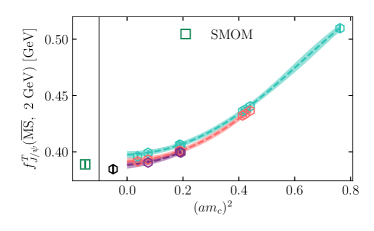
Figure 5: Continuum extrapolation of the $J/\psi$ tensor decay constant in the $\overline{\text{MS}}$ scheme at a scale of 2 GeV using an intermediate nonperturbative renormalisation of the tensor current in the RI^′-MOM scheme on the lattice. Multiple values of the renormalisation scale $\mu$ have been used so that $\mu$ dependent nonperturbative effects can be removed in the fit. The blue points and line are for $\mu=2$ GeV, orange for 3 GeV and purple for 4 GeV. The value obtained in the continuum limit with the condensate terms removed is shown as a black hexagon. The result is in agreement with that using RI-SMOM renormalisation (Figure 3) which is shown as the green square.

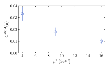
Figure 6: The same as Fig. 4 but for a correction term, $C^{\text{MOM}}(\mu)$, needed for the tensor current renormalisation factor when using the intermediate RI^′-MOM scheme.

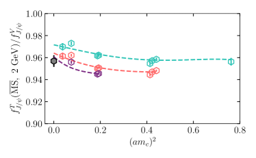
Figure 7: Continuum extrapolation of the ratio of the tensor and vector $J/\psi$ decay constants using intermediate lattice renormalisation factors in the RI-SMOM scheme. Blue points and lines show $\mu=2$ GeV results and fit lines, orange are 3 GeV and purple 4 GeV. The bold dashed lines are continuum extrapolations at each $\mu$ value with the condensate and $\alpha_{s}^{4}$ terms left in. The black hexagon is the continuum extrapolation with condensates and $\alpha_{s}^{4}$ errors removed.

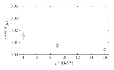
Figure 8: Correction $C^{\mathrm{SMOM}}(\mu)$ for the tensor current renormalisation factor, $Z_{T}$, determined from a fit to the ratio of the $J/\psi$ tensor and vector decay constants using intermediate renormalisation factors in the RI-SMOM scheme. This agrees with the results shown in Fig. 4, as expected because the lattice RI-SMOM vector current renormalisation factor has no condensate contamination Hatton et al. (2019).

Table 7: Error budget for the ratio of the $J/\psi$ vector and tensor decay constants. ‘Statistics’, the dominant uncertainty, refers to statistical errors in the amplitudes needed for the decay constants. The uncertainties coming from the renormalisation factors, $Z_{T}$ and $Z_{V}$, are much smaller and are dominated by the contribution from the (doubled) statistical uncertainties on the low statistics ultrafine lattices, set 8. The ‘Missing $\alpha_{s}^{4}$’ and ‘Condensates’ error contributions come from the terms in the fit from which the $Z_{T}$ correction (discussed in the text) is constructed.

	$f_{J/\psi}^{T}/f^{V}_{J/\psi}$
$(am_{c})^{2}\to 0$	0.11
$(\tilde{a}\mu)^{2}\to 0$	0.27
$Z_{T}$	0.12
$Z_{V}$	0.14
Missing $\alpha_{s}^{4}$ term	0.06
Statistics	0.41
Sea mistuning	0.04
Condensates	0.07
Total	0.54

Since the discretisation effects in $f_{J/\psi}^{T}$ are similar to those in $f_{J/\psi}^{V}$ on the same set of gluon field ensembles we expect to be able to extract the ratio of the two decay constants to a higher precision than can be obtained from the individual quantities. We may also be able to see a clearer indication of the size of nonperturbative effects in the ratio.

We show the ratio of $f^{T}/f^{V}$ in Fig. 7 using $Z_{T}$ and $Z_{V}$ determined in the RI-SMOM scheme. We neglect any correlations between the raw values of the decay constants on each lattice ensemble because the statistical uncertainties are so small. We fit the values of the ratio to Eq. (16) and obtain a result for the ratio in the continuum limit with nonperturbative contamination effects removed of:

$$\frac{f_{J/\psi}^{T}(\overline{\text{MS}},2\ \mathrm{GeV})}{f^{V}_{J/\psi}}=0.9569(52)\ \ \mathrm{(int.\,SMOM)}.$$ (20)

The fit has a $\chi^{2}/\mathrm{dof}$ of 0.2.

As discussed in Hatton et al. (2019) the RI-SMOM $Z_{V}$ contains no nonperturbative contamination because of the protection of the Ward-Takahashi identity and likewise no perturbative matching of SMOM to $\overline{\text{MS}}$ is needed. Therefore the condensate and $\alpha_{s}^{4}$ terms returned by the fit to the ratio of the tensor and vector $J/\psi$ decay constants should agree with those from the fit to just the tensor decay constant. We find that this is the case for each coefficient individually and for the $Z_{T}$ correction factor obtained from their combination which we show for the ratio fit in Fig. 8.

Because the RI^′-MOM determination of $Z_{V}$ has condensate contamination (since it is not protected by a Ward-Takahashi identity Hatton et al. (2019)) and perturbative matching is needed to reach $\overline{\text{MS}}$ we cannot perform the same analysis for that case.

We give an error budget for our result for the decay constant ratio $f_{J/\psi}^{T}/f^{V}_{J/\psi}$ in Table 7. We can leverage this ratio and the vector decay constant determined in Hatton et al. (2020) to get a slightly more precise value of the tensor decay constant:

$$f^{T}_{J/\psi}(\overline{\text{MS}},2\ \mathrm{GeV})=0.3927(27)\ \mathrm{GeV}\ \ (\mathrm{int.\,SMOM}).$$ (21)

The vector decay constant result of Hatton et al. (2019) includes QED effects from the non-zero electric charge of the valence charm quarks. We have not included any electromagnetic effects here. However, the QED effect on the vector decay constant was at the 0.2% level and we expect some cancellation of these effects in the decay constant ratio, so we neglect these effects here.

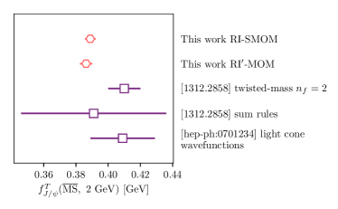
Figure 9: A comparison plot of results for the tensor $J/\psi$ decay constant in the $\overline{\text{MS}}$ scheme at a scale of 2 GeV. The top two results are from this work (using both RI-SMOM (Eq. (21)) and RI^′-MOM (Eq. (19)) intermediate schemes) and then we include results from Bečirević et al. (2014) and Braguta (2007).

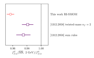
Figure 10: A comparison plot of results for the ratio of tensor and vector $J/\psi$ decay constants. The upper result is from this work (Eq. (20)) using the RI-SMOM intermediate scheme and gives a value significantly below 1 (marked with the black dashed line) for this ratio. The lower two results are from Bečirević et al. (2014).

V Discussion: $f_{J/\psi}^{T}$

As discussed in Section I there is no experimental observable available to which we can compare our tensor current decay constant value. Theoretical results using light-cone wavefunctions were presented in Braguta (2007) and using QCD sum rules in Bečirević et al. (2014). A lattice QCD result using twisted-mass quarks on gluon field ensembles with only $u/d$ quarks in the sea ($n_{f}=2$) was also given in Bečirević et al. (2014). The RI^′-MOM scheme was used to renormalise the lattice tensor and vector currents in that case, without studying or removing nonperturbative condensate contamination. We compare our results to these in Fig. 9 where the reduction in uncertainty that we have achieved here can clearly be seen.

A comparison plot of values of the decay constant ratio $f_{J/\psi}^{T}(2\,\mathrm{GeV})/f^{V}_{J/\psi}$ is shown in Fig. 10. This ratio is expected to be below 1 Bečirević et al. (2014) but we see that earlier results were not able to demonstrate this conclusively. Our value for the ratio is 8$\sigma$ below 1. The value that we obtain for the ratio is just over $1\sigma$ lower than the sum rules determination of Bečirević et al. (2014) and is over $2\sigma$ lower than the lattice QCD result of that work (using their $\sigma$ values). In the lattice QCD calculation both the tensor and vector current were renormalised in the RI^′-MOM scheme without accounting for nonperturbative contamination. Our results indicate that this could lead to a discrepancy with our results of the size seen.

VI Discussion: $Z_{T}$

Table 8: $Z_{T}$ values converting lattice results involving the tensor current to the $\overline{\text{MS}}$ scheme, run to a renormalisation scale of the $b$ quark pole mass. The notation $Z_{T}(\mu_{1}|\mu_{2})$ indicates that the intermediate $Z_{T}^{\text{SMOM}}$ has been calculated in the RI-SMOM scheme at a scale of $\mu_{1}$ and then converted to the $\overline{\mathrm{MS}}$ scheme and run to a scale of $\mu_{2}$. The superscript denotes that these renormalisation constants have been corrected for nonperturbative artefacts and $\alpha_{s}^{4}$ errors in $Z_{T}^{\text{SMOM}}$ as described in the text. The results with intermediate scales of 2 GeV and 3 GeV then agree well with each other and either can be used.

Set	$Z_{T}^{c}(2\ \mathrm{GeV}\ |\ m_{b})$	$Z_{T}^{c}(3\ \mathrm{GeV}\ |\ m_{b})$
vc	0.9493(42)	-
c	0.9740(43)	0.9707(25)
f	1.0029(43)	0.9980(25)
sf	1.0342(43)	1.0298(25)
uf	1.0476(42)	1.0456(25)

Table 9: Correlation matrix of the corrected $Z_{T}$ values from Table 8. These correlations are large because the matching, running and correction terms are all correlated.

	(vc,2)	(c,2)	(f,2)	(sf,2)	(uf,2)	(c,3)	(f,3)	(sf,3)	(uf,3)
(vc,2)	1.0	0.99750	0.99854	0.99475	0.93231	0.98398	0.98611	0.98713	0.96383
(c,2)	0.99750	1.0	0.99777	0.99430	0.93294	0.98314	0.98371	0.98487	0.96243
(f,2)	0.99854	0.99777	1.0	0.99605	0.93562	0.98045	0.98323	0.98423	0.96263
(sf,2)	0.99475	0.99430	0.99605	1.0	0.93197	0.97361	0.97632	0.98097	0.95627
(uf,2)	0.93231	0.93294	0.93562	0.93197	1.0	0.90439	0.90777	0.90941	0.96855
(c,3)	0.98398	0.98314	0.98045	0.97361	0.90439	1.0	0.99909	0.99807	0.96824
(f,3)	0.98611	0.98371	0.98323	0.97632	0.90777	0.99909	1.0	0.99868	0.96951
(sf,3)	0.98713	0.98487	0.98423	0.98097	0.90941	0.99807	0.99868	1.0	0.96909
(uf,3)	0.96383	0.96243	0.96263	0.95627	0.96855	0.96824	0.96951	0.96909	1.0

In the discussion presented above in Section IV we ran all of our results, after converting to $\overline{\mathrm{MS}}$, to a common scale of 2 GeV and then determined and subtracted a correction that depends on $\mu$. This correction needs to be applied to our $Z_{T}$ values for future use. The scale of 2 GeV allows us to compare directly to the results of Bečirević et al. (2014) in Section V. However, another scale is useful when computing form factors for semileptonic $B$ decay processes. Then differential rates are calculated as functions of products of the form factors and appropriate Wilson coefficients of the weak Hamiltonian. These Wilson coefficients are scale dependent and are typically calculated at a scale equal to the $b$ pole mass, 4.8 GeV, see for example Altmannshofer et al. (2009). We therefore present our $Z_{T}$ values run to this scale. If the $b$ quark running mass of 4.2 GeV were used instead of the pole mass then the values would be approximately 1% larger.

In Table 8 we give the corrected results for $Z_{T}$ in the $\overline{\mathrm{MS}}$ scheme at a scale equal to the $b$ quark pole mass calculated from intermediate values of $Z_{T}$ in the RI-SMOM scheme at 2 and 3 GeV. We use a notation $Z_{T}(\mu_{\mathrm{SMOM}}\ |\ \mu_{\overline{\mathrm{MS}}})$ where $\mu_{\mathrm{SMOM}}$ is the scale at which the RI-SMOM calculation was performed and $\mu_{\overline{\mathrm{MS}}}$ is the final scale at which the $\overline{\mathrm{MS}}$ result is presented. It can be seen that the addition of the correction results in $Z_{T}$ values that agree for different intermediate scales once run to the same final scale (this would not be true for uncorrected values). We also give the correlations between these numbers in Table 9.

VII Conclusions

We have shown here that it is possible to renormalise lattice tensor currents to give accurate results for continuum matrix elements in the $\overline{\text{MS}}$ scheme using nonperturbative determination of intermediate renormalisation factors in momentum-subtraction schemes. A key requirement is that the nonperturbative renormalisation factors should be obtained at multiple values of the renormalisation scale, $\mu$, so that $\mu$-dependent nonperturbative (condensate) contamination of $Z_{T}$ can be fitted and removed. This contamination would otherwise give a systematic error of 1.5% using the RI-SMOM scheme and 3% using the RI^′-MOM scheme in our calculation.

In order to do this we have determined the $J/\psi$ tensor decay constant, $f_{J/\psi}^{T}$ so that we can study the continuum limit of a tensor current matrix element. Using $n_{f}=2+1+1$ HISQ lattices and the local tensor current, we obtain a 0.7%-accurate value for $f_{J/\psi}^{T}$ of (repeating Eq. (21))

$$f^{T}_{J/\psi}(\overline{\text{MS}},2\ \mathrm{GeV})=0.3927(27)\ \mathrm{GeV}\ \ (\mathrm{int.\,SMOM}).$$ (22)

This uses our preferred intermediate RI-SMOM scheme and makes use of the determination of the ratio of tensor to vector decay constants and the fact that the vector current renormalisation is protected by the Ward-Takahashi identity in this scheme Hatton et al. (2019). We also obtain a 0.5%-accurate value for the ratio itself (repeating Eq. (20)),

$$\frac{f_{J/\psi}^{T}(\overline{\text{MS}},2\ \mathrm{GeV})}{f^{V}_{J/\psi}}=0.9569(52)\ \ (\mathrm{int.\,SMOM}).$$ (23)

This shows unequivocally that the ratio is less than 1.

Finally, in Tables 8 and 9, we give $Z_{T}$ renormalisation factors that can be used, for example, in a future determination (underway) of the tensor form factor for the rare flavour-changing neutral current process $B\rightarrow K\ell^{+}\ell^{-}$ using HISQ quarks. These $Z_{T}$ values take results determined with the local HISQ lattice tensor current and convert them into values in the $\overline{\text{MS}}$ scheme at the scale of $m_{b}$, to be multiplied by Wilson coefficients from the effective weak Hamiltonian determined at this scale. We have corrected these $Z_{T}$ values so that they are free of the systematic error from condensate contamination of the intermediate momentum-subtraction scheme.

Acknowledgements

We are grateful to the MILC collaboration for the use of their configurations and code. Computing was done on the Cambridge service for Data Driven Discovery (CSD3), part of which is operated by the University of Cambridge Research Computing on behalf of the DIRAC HPC Facility of the Science and Technology Facilities Council (STFC). The DIRAC component of CSD3 was funded by BEIS capital funding via STFC capital grants ST/P002307/1 and ST/R002452/1 and STFC operations grant ST/R00689X/1. DiRAC is part of the national e-infrastructure. We are grateful to the CSD3 support staff for assistance. Funding for this work came from the UK Science and Technology Facilities Council grants ST/L000466/1 and ST/P000746/1 and from the National Science Foundation.

References

- Hurth and Nakao (2010) T. Hurth and M. Nakao, Ann. Rev. Nucl. Part. Sci. 60, 645 (2010), arXiv:1005.1224 [hep-ph] .
- Bouchard et al. (2013) C. Bouchard, G. P. Lepage, C. Monahan, H. Na, and J. Shigemitsu (HPQCD), Phys. Rev. D88, 054509 (2013), [Erratum: Phys. Rev.D88,no.7,079901(2013)], arXiv:1306.2384 [hep-lat] .
- Bailey et al. (2016) J. A. Bailey et al., Phys. Rev. D93, 025026 (2016), arXiv:1509.06235 [hep-lat] .
- Follana et al. (2007) E. Follana, Q. Mason, C. Davies, K. Hornbostel, G. P. Lepage, J. Shigemitsu, H. Trottier, and K. Wong (HPQCD, UKQCD), Phys. Rev. D75, 054502 (2007), arXiv:hep-lat/0610092 [hep-lat] .
- McNeile et al. (2012a) C. McNeile, C. T. H. Davies, E. Follana, K. Hornbostel, and G. P. Lepage, Phys. Rev. D85, 031503 (2012a), arXiv:1110.4510 [hep-lat] .
- McNeile et al. (2012b) C. McNeile, C. T. H. Davies, E. Follana, K. Hornbostel, and G. P. Lepage, Phys. Rev. D86, 074503 (2012b), arXiv:1207.0994 [hep-lat] .
- McLean et al. (2019) E. McLean, C. T. H. Davies, A. T. Lytle, and J. Koponen, Phys. Rev. D99, 114512 (2019), arXiv:1904.02046 [hep-lat] .
- McLean et al. (2020) E. McLean, C. Davies, J. Koponen, and A. Lytle, Phys. Rev. D 101, 074513 (2020), arXiv:1906.00701 [hep-lat] .
- Martinelli et al. (1995) G. Martinelli, C. Pittori, C. T. Sachrajda, M. Testa, and A. Vladikas, Nucl. Phys. B 445, 81 (1995), arXiv:hep-lat/9411010 .
- Lytle et al. (2018) A. T. Lytle, C. T. H. Davies, D. Hatton, G. P. Lepage, and C. Sturm (HPQCD), Phys. Rev. D98, 014513 (2018), arXiv:1805.06225 [hep-lat] .
- Hatton et al. (2020) D. Hatton, C. Davies, B. Galloway, J. Koponen, G. Lepage, and A. Lytle, (2020), arXiv:2005.01845 [hep-lat] .
- Bečirević et al. (2014) D. Bečirević, G. Duplančić, B. Klajn, B. Melić, and F. Sanfilippo, Nucl. Phys. B883, 306 (2014), arXiv:1312.2858 [hep-ph] .
- Hazard and Petrov (2016) D. E. Hazard and A. A. Petrov, Phys. Rev. D94, 074023 (2016), arXiv:1607.00815 [hep-ph] .
- Grinstein and Martin Camalich (2016) B. Grinstein and J. Martin Camalich, Phys. Rev. Lett. 116, 141801 (2016), arXiv:1509.05049 [hep-ph] .
- Chetyrkin and Retey (2000) K. Chetyrkin and A. Retey, Nucl. Phys. B 583, 3 (2000), arXiv:hep-ph/9910332 .
- Aoki et al. (2008) Y. Aoki et al., Phys. Rev. D 78, 054510 (2008), arXiv:0712.1061 [hep-lat] .
- Sturm et al. (2009) C. Sturm, Y. Aoki, N. Christ, T. Izubuchi, C. Sachrajda, and A. Soni, Phys. Rev. D 80, 014501 (2009), arXiv:0901.2599 [hep-ph] .
- Gattringer et al. (2004) C. Gattringer, M. Gockeler, P. Huber, and C. B. Lang, Nucl. Phys. B694, 170 (2004), arXiv:hep-lat/0404006 [hep-lat] .
- Constantinou et al. (2016) M. Constantinou, M. Hadjiantonis, H. Panagopoulos, and G. Spanoudes, Phys. Rev. D94, 114513 (2016), arXiv:1610.06744 [hep-lat] .
- Gracey (2000) J. Gracey, Phys. Lett. B 488, 175 (2000), arXiv:hep-ph/0007171 .
- Chakraborty et al. (2015) B. Chakraborty, C. T. H. Davies, B. Galloway, P. Knecht, J. Koponen, G. C. Donald, R. J. Dowdall, G. P. Lepage, and C. McNeile, Phys. Rev. D91, 054508 (2015), arXiv:1408.4169 [hep-lat] .
- Borsanyi et al. (2012) S. Borsanyi, S. Durr, Z. Fodor, C. Hoelbling, S. D. Katz, et al., JHEP 1209, 010 (2012), arXiv:1203.4469 [hep-lat] .
- Dowdall et al. (2013) R. Dowdall, C. Davies, G. Lepage, and C. McNeile (HPQCD), Phys.Rev. D88, 074504 (2013), arXiv:1303.1670 [hep-lat] .
- Almeida and Sturm (2010) L. G. Almeida and C. Sturm, Phys. Rev. D 82, 054017 (2010), arXiv:1004.4613 [hep-ph] .
- Kniehl and Veretin (2020) B. A. Kniehl and O. L. Veretin, Phys. Lett. B 804, 135398 (2020), arXiv:2002.10894 [hep-ph] .
- Gracey (2003) J. A. Gracey, Nucl. Phys. B662, 247 (2003), arXiv:hep-ph/0304113 [hep-ph] .
- Franco and Lubicz (1998) E. Franco and V. Lubicz, Nucl. Phys. B531, 641 (1998), arXiv:hep-ph/9803491 [hep-ph] .
- Chetyrkin and Maier (2010) K. Chetyrkin and A. Maier, JHEP 01, 092 (2010), arXiv:0911.0594 [hep-ph] .
- Gorbahn and Jager (2010) M. Gorbahn and S. Jager, Phys. Rev. D82, 114001 (2010), arXiv:1004.3997 [hep-ph] .
- Bi et al. (2018) Y. Bi, H. Cai, Y. Chen, M. Gong, K.-F. Liu, Z. Liu, and Y.-B. Yang, Phys. Rev. D 97, 094501 (2018), arXiv:1710.08678 [hep-lat] .
- Lytle and Sharpe (2013) A. T. Lytle and S. R. Sharpe, Phys. Rev. D 88, 054506 (2013), arXiv:1306.3881 [hep-lat] .
- Arthur and Boyle (2011) R. Arthur and P. A. Boyle (RBC, UKQCD), Phys. Rev. D83, 114511 (2011), arXiv:1006.0422 [hep-lat] .
- Bazavov et al. (2010) A. Bazavov et al. (MILC), Phys. Rev. D82, 074501 (2010), arXiv:1004.0342 [hep-lat] .
- Bazavov et al. (2013) A. Bazavov et al. (MILC), Phys. Rev. D87, 054505 (2013), arXiv:1212.4768 [hep-lat] .
- Hatton et al. (2019) D. Hatton, C. Davies, G. Lepage, and A. Lytle (HPQCD), Phys. Rev. D 100, 114513 (2019), arXiv:1909.00756 [hep-lat] .
- Lepage et al. (2002) G. P. Lepage, B. Clark, C. T. H. Davies, K. Hornbostel, P. B. Mackenzie, C. Morningstar, and H. Trottier, Lattice field theory. Proceedings, 19th International Symposium, Lattice 2001, Berlin, Germany, August 19-24, 2001, Nucl. Phys. Proc. Suppl. 106, 12 (2002), arXiv:hep-lat/0110175 [hep-lat] .
- Braguta (2007) V. Braguta, Phys. Rev. D 75, 094016 (2007), arXiv:hep-ph/0701234 .
- Altmannshofer et al. (2009) W. Altmannshofer, P. Ball, A. Bharucha, A. J. Buras, D. M. Straub, and M. Wick, JHEP 01, 019 (2009), arXiv:0811.1214 [hep-ph] .