Young stellar cluster dilution near supermassive black holes:
the impact of Vector Resonant Relaxation on neighbour separation

Abstract

We investigate the rate of orbital orientation dilution of young stellar clusters in the vicinity of supermassive black holes. Within the framework of vector resonant relaxation, we predict the time evolution of the two-point correlation function of the stellar orbital plane orientations as a function of their initial angular separation and diversity in orbital parameters (semi-major axis, eccentricity). As expected, the larger the spread in initial orientations and orbital parameters, the more efficient the dilution of a given set of co-eval stars, with a characteristic timescale set up by the coherence time of the background potential fluctuations. A Markovian prescription which matches numerical simulations allows us to efficiently probe the underlying kinematic properties of the unresolved nucleus when requesting consistency with a given dilution efficiency, imposed by the observed stellar disc within the one arcsecond of Sgr A*. As a proof of concept, we compute maps of constant dilution times as a function of the semi major axis cusp index and fraction of intermediate mass black holes in the old background stellar cluster. This computation suggests that vector resonant relaxation should prove useful in this context since it impacts orientations on timescales comparable to the stars’ age.

1 Introduction

Most nearby galaxies harbour a supermassive black hole (BH) in their centre, surrounded by a dense stellar cluster (Genzel et al., 2010; Kormendy & Ho, 2013). In the last few years, outstanding instrumental developments have led to observational breakthrough in this context: the strings of gravitational wave detections following the coalescence of black holes (Abbott et al., 2016), the first shadow image of the horizon via radio interferometry of M87 (Event Horizon Telescope Collab. et al., 2019), as well as the first measurement of the relativistic precession of stars in our own Galaxy (Gravity Collab. et al., 2020). These past successes should undoubtedly be followed by others, accompanying the upcoming thirty meter-class optical instruments (Do et al., 2019) and space interferometry (Berti et al., 2006). These datasets will allow us to put more stringent constraints on the vicinity of massive black holes embedded in galactic centres, e.g., to identify dark relics such as intermediate mass black holes (Portegies Zwart & McMillan, 2002).

Owing to the infinite potential well generated by the central BH, galactic nuclei, even in isolation, are stellar systems that involve a wide range of dynamical timescales and processes (Rauch & Tremaine, 1996; Hopman & Alexander, 2006; Alexander, 2017). (i) Since the BH dominates the gravitational potential, stars follow nearly Keplerian ellipses. This is the dynamical time. (ii) The deviations from a Keplerian potential due to the stellar mass and relativistic corrections lead to the in-plane precessions of the Keplerian ellipses. This is the precession time. (iii) Subsequently, because of the non-spherical components of the potential fluctuations, the orbital orientations of the stars get reshuffled. The Keplerian ellipses’ angular momentum vectors change in orientations, without changing in magnitude (i.e. eccentricity) nor in energy (i.e. semi-major axis). This is the timescale for vector resonant relaxation (VRR) (Kocsis & Tremaine, 2015; Fouvry et al., 2019b, and references therein). (iv) On longer timescales, resonant torques between the precessing stars lead to a diffusion of the stars’ angular momentum magnitude. This is the timescale for scalar resonant relaxation (SRR) (Bar-Or & Fouvry, 2018, and references therein). (v) Finally, on the longest timescale, the slow build-up of close encounters between stars allow for the relaxation of their Keplerian energy. This is the timescale for non-resonant relaxation (NR) (Bahcall & Wolf, 1976; Cohn & Kulsrud, 1978; Shapiro & Marchant, 1978; Bar-Or & Alexander, 2016; Vasiliev, 2017).

In the present paper, we are interested in the process of VRR as an astrophysical tool to probe the structure of galactic centres. This dynamical process, through which stars see their orbital orientations vary, plays a crucial role in numerous dynamical phenomena in galactic nuclei. Indeed, VRR allows for example for the warping of stellar discs (Kocsis & Tremaine, 2011), or for the enhancement of binary mergers rates (Hamers et al., 2018). Moreover, because it is the only mechanism that can efficiently shuffle orbital orientations, a detailed study of VRR is also a mandatory step to understand the formation and survival of anisotropic, i.e. non-spherical, structures in galactic nuclei. This is in particular the case of the ‘clockwise’ disc observed within SgrA* (Bartko et al., 2009; Yelda et al., 2014; Gillessen et al., 2017), whose presence constrains the efficiency with which VRR can dissolve anisotropic stellar structures.

Following its first description in Rauch & Tremaine (1996), VRR has been extensively studied in various ways. It was tackled using full numerical simulations (Eilon et al., 2009), orbit-averaged simulations (Kocsis & Tremaine, 2015), as well as kinetic predictions (Fouvry et al., 2019b, a). Because VRR is a rather fast dynamical process (${\sim 10^{6}\,\mathrm{yr}}$ for the S-cluster of SgrA*), it also prove important to characterise the thermodynamical equilibria of that process (Roupas et al., 2017; Takács & Kocsis, 2018; Tremaine, 2020). On that front, Szölgyén & Kocsis (2018) recently showed how VRR equilibria can exhibit strong anisotropic mass segregation leading to the formation of black hole discs in galactic nuclei.

In the present paper, we set out to characterise the efficiency with which VRR can lead to the dissolution of anisotropic stellar structures in galactic nuclei, building upon Fouvry et al. (2019b). As such, we are interested in determining how efficiently stars with similar orbital orientations, e.g., stars orbiting within the same stellar disc, can diffuse away from each other as a result of the VRR process. We call this process ‘neighbour separation’. The paper is organised as follows. In section 2, we recall the key equations of VRR, as well as the statistical properties of the potential fluctuations present in the system. In section 3, we compute the average rate of separation of two nearby test stars. Section 4 relies on a Markovian assumption to improve upon this prediction to capture the (very) slow dilution of (very) similar orientations, while Appendix I shows how one can design an effective Markov process to generate virtual separations that statistically match that dynamics. In section 5, we subsequently illustrate how this formalism can be used to put constraints on the unresolved cluster orbiting a super massive BH in a setting inspired by the SgrA*’s stellar disc. Finally, we conclude in section 6.

Details of the involved calculations or numerical validations are spread through appendices. In particular, we present a toy model (Appendix H) which allows us to both qualitatively capture key aspects of VRR, and produce virtual dilutions of neighbour test stars.

2 VRR dynamics

We consider a set of ${N\gg 1}$ stars orbiting a supermassive BH of mass $M_{\bullet}$, that we call the background bath of particles. They represent the unresolved population (low mass stars, intermediate mass black holes, etc) which contribute to the clumpiness of the gravitational potential. Provided that one considers the dynamics of stars on timescales longer than the in-plane precession, but shorter than the relaxation time for eccentricity (by SRR) and energy (by NR), one can smear out stars along their respective mean anomalies and pericentre phase. After this double orbit-average, stars are replaced by annuli, extending between the pericentre and apocentre of every stellar orbit. as illustrated in Fig. 1.

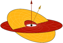
Figure 1: Illustration of the interaction between two annuli with different orbital parameters ${\mathbf{K}=(m,a,e)}$. The torque between the two annuli only depends on the relative angle, ${\cos(\phi)}$, between the two normals. VRR predicts the process through which the orientation of these orbital annuli diffuse in time.

To every annuli is then associated a set of conserved quantities ${\mathbf{K}=(m,a,e)}$, with $m$ the individual mass, $a$ the semi-major axis, and $e$ the eccentricity. In that limit, the only remaining dynamical quantity is the instantaneous orbital orientation given by the unit vector $\widehat{\mathbf{L}}$. VRR  then describes the dynamics of a set of long-range coupled unit vectors ${\widehat{\mathbf{L}}_{i}}$.

2.1 Hamiltonian of VRR

Following the notations from Fouvry et al. (2019b), the effective single-particle Hamiltonian of VRR reads

$$H=-\sum_{j=1}^{N}\bigg{\langle}\frac{Gmm_{j}}{|\mathbf{x}(t)-\mathbf{x}_{j}(t^{\prime})|}\bigg{\rangle}_{t,t^{\prime}},$$ (1)

where the sum over $j$ runs over all the background particles, and the average ${\langle\,\rangle_{t,t^{\prime}}}$ operates over the fast Keplerian motions and the in-plane precessions of both the test particle, and the background particles, hereby replacing stars with annuli.

Following Eq. (1) of Fouvry et al. (2019b), this Hamiltonian can be rewritten under the shorter form

$$H=-L(\mathbf{K})\sum_{j=1}^{N}\sum_{\mathclap{\begin{subarray}{c}\ell\geq 2\\ \mathrm{even}\end{subarray}}}\,\,\sum_{\mathclap{m=-\ell}}^{\ell}\mathcal{J}_{\ell}\big{[}\mathbf{K},\mathbf{K}_{j}\big{]}\,Y_{\ell m}(\widehat{\mathbf{L}})\,Y_{\ell m}(\widehat{\mathbf{L}}_{j}(t)),$$ (2)

where ${\widehat{\mathbf{L}}(t)}$ stands for the instantaneous orbital orientation of the test particle, and ${\widehat{\mathbf{L}}_{j}(t)}$ for that of the bath particles. Similarly, $\mathbf{K}$ is the conserved parameter of the test particle, and $\mathbf{K}_{j}$ the ones of the bath particle. In Eq. (2), we also introduced the norm of the angular momentum as ${L(\mathbf{K})=m\sqrt{GM_{\bullet}a(1-e^{2})}}$. The coupling coefficients, ${\mathcal{J}_{\ell}[\mathbf{K},\mathbf{K}_{j}]}$, depend only on the stars’ conserved parameters, and are constant throughout the VRR dynamics. Their detailed expressions are recalled in Appendix A. Finally, in Eq. (2), we also introduced the real spherical harmonics, ${Y_{\ell m}(\widehat{\mathbf{L}})}$, defined with the normalisation ${\!\int\!\mathrm{d}\widehat{\mathbf{L}}\,Y_{\ell m}Y_{\ell^{\prime}m^{\prime}}\!=\!\delta_{\ell\ell^{\prime}}\delta_{mm^{\prime}}}$.

The instantaneous state of the background bath is fully described by the discrete distribution function (DF)

$$f^{\mathrm{b}}(\widehat{\mathbf{L}},\mathbf{K},t)=\sum_{j=1}^{N}\delta_{\mathrm{D}}(\widehat{\mathbf{L}}-\widehat{\mathbf{L}}_{j}(t))\,\delta_{\mathrm{D}}(\mathbf{K}-\mathbf{K}_{j}).$$ (3)

It can naturally be expanded in spherical harmonics as

$$f^{\mathrm{b}}(\widehat{\mathbf{L}},\mathbf{K},t)=f^{\mathrm{b}}_{\alpha}(\mathbf{K},t)\,Y_{\alpha}(\widehat{\mathbf{L}}),$$ (4)

where the sum over ${\alpha=(\ell_{\alpha},m_{\alpha})}$ is implied, and we wrote

$$f^{\mathrm{b}}_{\alpha}(\mathbf{K},t)=\sum_{j=1}^{N}\delta_{\mathrm{D}}(\mathbf{K}-\mathbf{K}_{j})\,Y_{\alpha}(\widehat{\mathbf{L}}_{j}(t)).$$ (5)

As already derived in Eq. (9) of Fouvry et al. (2019b), the harmonics of the bath evolve according to

$$\frac{\partial f^{\mathrm{b}}_{\alpha}(\mathbf{K},t)}{\partial t}\!=\!-\!\!\int\!\!\mathrm{d}\mathbf{K}^{\prime}\,\mathcal{J}_{\gamma}\big{[}\mathbf{K},\mathbf{K}^{\prime}\big{]}E_{\alpha\gamma\delta}f^{\mathrm{b}}_{\gamma}(\mathbf{K}^{\prime},t)f^{\mathrm{b}}_{\delta}(\mathbf{K},t).$$ (6)

In that expression, the sum over the harmonic indices ${\gamma,\delta}$ is implied, recalling that the coupling coefficient, $\mathcal{J}_{\gamma}$, only depends on $\ell_{\gamma}$. We also introduced the (constant) Elsasser coefficients, $E_{\alpha\gamma\delta}$, whose properties are presented in Appendix B. Equation (6) is the fundamental equation of VRR and describes exactly that dynamics. The complexity of Eq. (6) comes from the fact that it is a quadratic matrix differential equation for fields.

2.2 Noise in VRR

Rather than describing the exact fate of all the bath particles, we aim at characterising the statistical properties of the coefficients ${f^{\mathrm{b}}_{\alpha}(\mathbf{K},t)}$. This was done in Fouvry et al. (2019b), and we recall here the key equations.

As they are self-consistently generated by ${N\gg 1}$ particles, we can assume via the central limit theorem that ${f^{\mathrm{b}}_{\alpha}(\mathbf{K},t)}$ is a Gaussian random field. If we also assume that the bath’s evolution is stationary in time, these stochastic fields are fully characterised by their correlation function

$$C^{\mathrm{b}}_{\alpha\beta}(\mathbf{K},\mathbf{K}^{\prime},t-t^{\prime})=\big{\langle}f^{\mathrm{b}}_{\alpha}(\mathbf{K},t)\,f^{\mathrm{b}}_{\beta}(\mathbf{K}^{\prime},t)\big{\rangle},$$ (7)

where ${\langle\,\cdot\,\rangle}$ stands for the ensemble average over realisations, i.e. over the initial conditions of the bath. Fouvry et al. (2019b) showed that these correlation functions can be well approximated by temporal Gaussians of the form

$$C^{\mathrm{b}}_{\alpha\beta}(\mathbf{K},\mathbf{K}^{\prime},t\!-\!t^{\prime})\!=\!\delta_{\alpha\beta}\delta_{\mathrm{D}}(\mathbf{K}\!-\!\mathbf{K}^{\prime})n(\mathbf{K})\mathrm{e}^{-\frac{A_{\ell_{\alpha}}}{2}(t/T_{\mathrm{c}}(\mathbf{K}))^{2}},$$ (8)

with the coefficient ${A_{\ell}\!=\!\ell(\ell\!+\!1)}$. In that expression, it was also assumed that the background bath is, on average, isotropic, and we introduced the DF of the stars’ parameters, ${n(\mathbf{K})}$, with the normalisation convention ${\!\int\!\mathrm{d}\widehat{\mathbf{L}}\mathrm{d}\mathbf{K}n(\mathbf{K})=N}$. This DF is the quantity we aim to constrain using VRR.

Equation (8) fully characterises the statistical properties of the potential fluctuations generated by the background particles. We note that the amplitude of its temporal correlation is proportional to the background’s stellar density, ${n(\mathbf{K})}$. As the system is isotropic on average, these correlations are diagonal when expanded in spherical harmonics, and only depend on the index $\ell$. Finally, in Eq. (8), we also introduced the coherence time of the noise, ${T_{\mathrm{c}}(\mathbf{K})}$, that follows from Eq. (19) of Fouvry et al. (2019b) and reads

$$\frac{1}{T_{\mathrm{c}}^{2}(\mathbf{K})}=\!\!\int\!\!\mathrm{d}\mathbf{K}^{\prime}\,n(\mathbf{K}^{\prime})\sum_{\ell}B_{\ell}\,\mathcal{J}_{\ell}^{2}\big{[}\mathbf{K},\mathbf{K}^{\prime}\big{]},$$ (9)

with the constant coefficient ${B_{\ell}\!=\!\ell(\ell\!+\!1)(2\ell\!+\!1)/(8\pi)}$. The coherence time characterises the time one has to wait for the bath to reshuffle enough so that its fluctuations become statistically independent. As highlighted in the coming section, this timescale will also set the typical timescale on which neighbouring test particles will be able to drift away from one another.

3 neighbour separation

In this section, we now tackle the problem of describing the simultaneous separation of two test stars sharing similar orientations and parameters.

3.1 Dynamics of test particles

Let us consider therefore two test (or tracer) particles, resp. indexed by ‘$1$’ and ‘$2$’. They represent here stars which are bright enough to be observed, while the background bath corresponds to the unresolved old stellar cluster (possibly involving black holes), too dim to be directly imaged. We place ourselves in the test particle limit, i.e. we assume that the motions of the test particles are fully imposed by the background bath (in the so-called zero mass limit). As such, we neglect any back-reaction of these particles on the bath, and we neglect any self-gravity between the two test particles. This effectively halves the Hamiltonian and allows for the statistics given by Eq. (8) to be used in our subsequent calculations. As a result, the background bath is therefore fully self-gravitating, i.e. follows the dynamics imposed by the Hamiltonian from Eq. (1), while the test particles are only probing the gravitational potential in the cluster but do not contribute to it. Our goal is now to constrain the efficiency with which a young stellar cluster (i.e. the test particles) can dissolve as a result of the potential fluctuations generated by the old unresolved stellar cluster (i.e. the background bath). In Fig. 2, we illustrate one example of such a dilution in a numerical simulation.

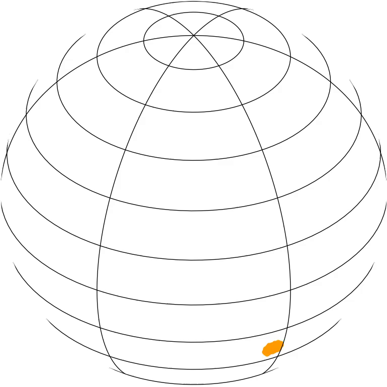
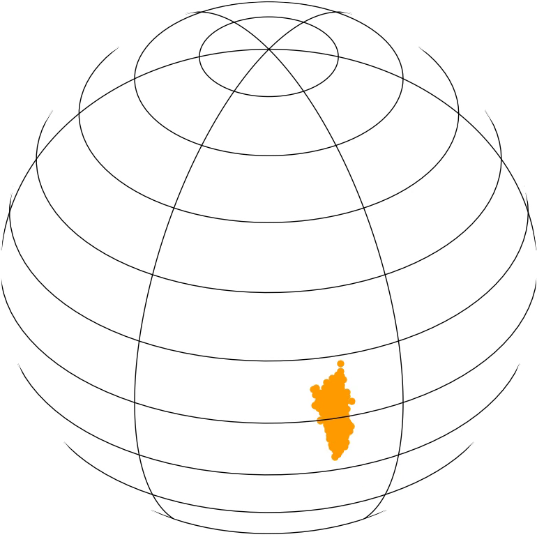
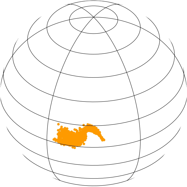
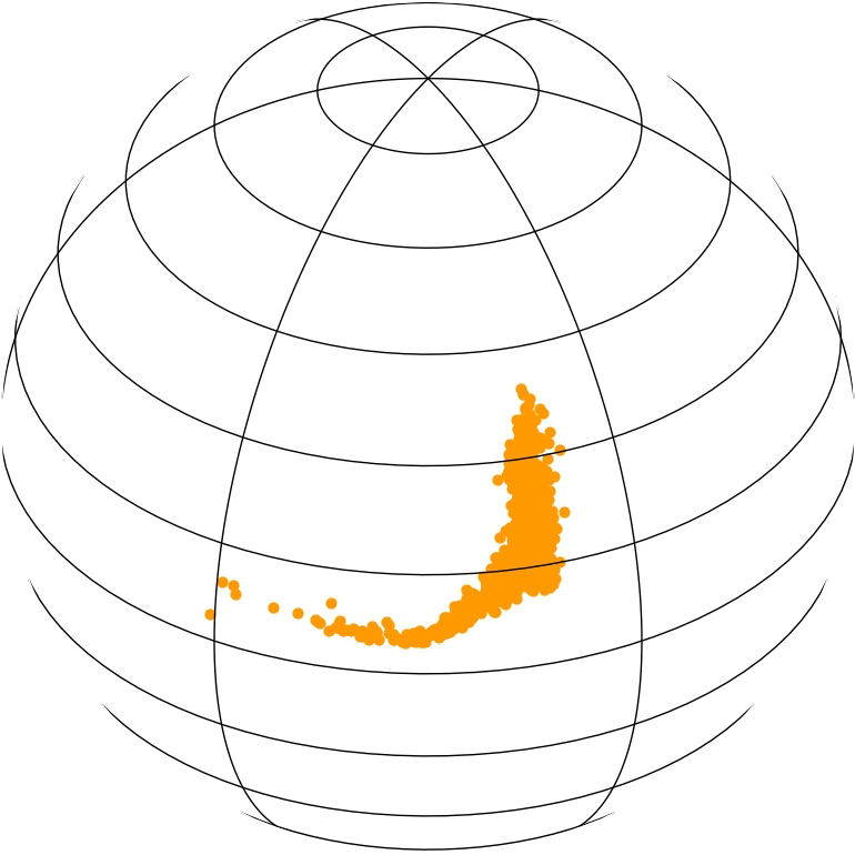
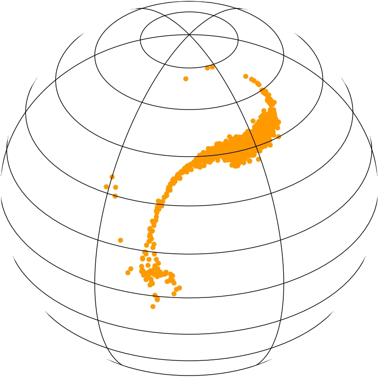
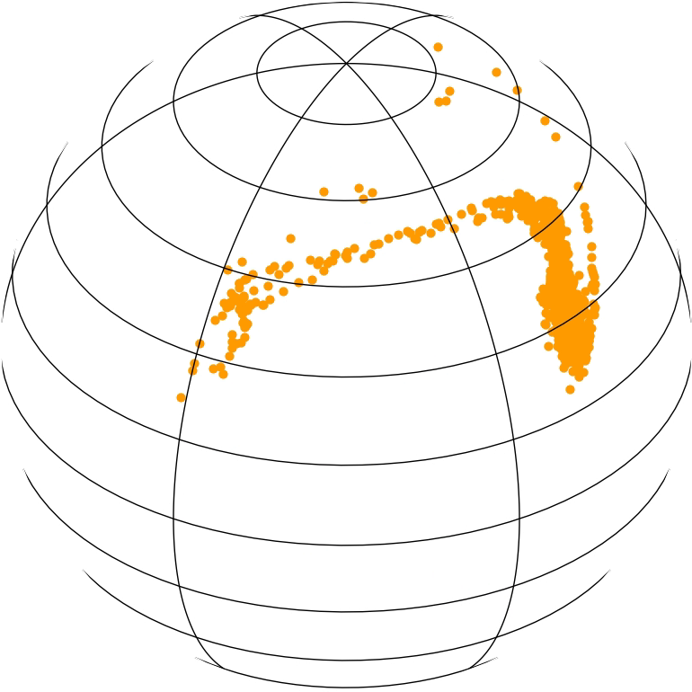
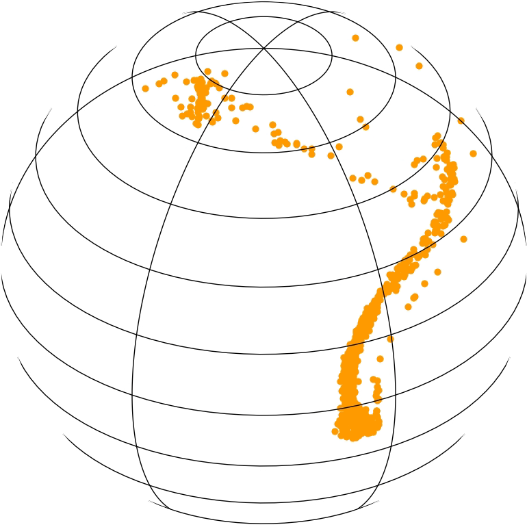
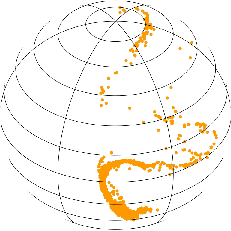
Figure 2: Illustration of the separations between neighbouring tracer particles, differing initially both in orientations and orbital parameters. Details for this simulation are spelled out in Appendix F. This time sequence (from left to right and top to bottom) shows that a patch of orbital planes initially close to each other diffuses while interacting with the background unresolved cluster. The patch becomes quite elongated, as a result of the phase space shearing generated by the instantaneous potential fluctuations. Similarly, the patch also moves somewhat faster than it spreads. Eventually, the test particles will become distributed over the whole sphere.

We denote the parameters of the test particles with ${\mathbf{K}_{i}}$ (with ${i=1,2}$) and their current orientation with ${\widehat{\mathbf{L}}_{i}(t)}$. Similarly to Eq. (3), each test particle is fully characterised by its probability distribution function (PDF)

$$f^{i}(\widehat{\mathbf{L}},t)=\delta_{\mathrm{D}}(\widehat{\mathbf{L}}-\widehat{\mathbf{L}}_{i}(t)).$$ (10)

It can naturally be expanded in spherical harmonics as ${f^{i}(\widehat{\mathbf{L}},t)=f^{i}_{\alpha}(t)Y_{\alpha}(\widehat{\mathbf{L}})}$, where the sum over $\alpha$ is implied. Here, the harmonics decomposition simply reads

$$f^{i}_{\alpha}(t)=Y_{\alpha}(\widehat{\mathbf{L}}_{i}(t)).$$ (11)

Because the test particles do not contribute to the system’s instantaneous potential, their individual dynamics follow from Eq. (6) and take the simpler form

$$\frac{\partial f_{\alpha}^{i}(t)}{\partial t}=-\!\!\int\!\!\mathrm{d}\mathbf{K}\,\mathcal{J}_{\gamma}\big{[}\mathbf{K}_{i},\mathbf{K}\big{]}\,E_{\alpha\gamma\delta}\,f^{\mathrm{b}}_{\gamma}(\mathbf{K},t)\,f^{i}_{\delta}(t),$$ (12)

where, once again, the sums over ${\gamma,\delta}$ are implied. In order to better highlight its properties, we can finally rewrite Eq. (12) as

$$\frac{\partial f_{\alpha}^{i}(t)}{\partial t}=-Q_{\alpha\delta}^{i}(t)\,f^{i}_{\delta}(t),$$ (13)

where ${Q_{\alpha\delta}^{i}(t)\!=\!\!\int\!\mathrm{d}\mathbf{K}\mathcal{J}_{\gamma}[\mathbf{K}_{i},\mathbf{K}]E_{\alpha\gamma\delta}f^{\mathrm{b}}_{\gamma}(\mathbf{K},t)}$ is a stochastic matrix because ${f^{\mathrm{b}}_{\gamma}(\mathbf{K},t)}$ is a stochastic field, whose statistical properties were already spelled out in Eq. (8). Equation (13) now takes the form of a set of coupled linear differential equations, sourced by the fluctuations of the background bath through the time-dependent matrix ${\mathbf{Q}_{i}(t)}$. Let us emphasise that the matrices ${\mathbf{Q}_{i}(t)}$ are indexed by the test particles’ index, $i$, as they depend on their conserved parameters $\mathbf{K}_{i}$. Yet, ${\mathbf{Q}_{i}(t)}$ and ${\mathbf{Q}_{j}(t)}$ are highly correlated one with another, as they both depend on the same instantaneous fluctuations ${f^{\mathrm{b}}_{\gamma}(\mathbf{K},t)}$ generated by the bath. It is essential to accurately capture these correlations in order to describe the process of neighbour separation.

3.2 Correlation of separation

Having written in Eq. (12) the exact evolution equation for the test particles, we can now address the computation of their rate of separation.

We are interested in the efficiency with which two nearby particles diffuse away from each other. We illustrate such a separation in Fig. 3.

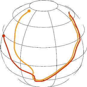
Figure 3: Illustration of separation between two neighbouring tracer particles. The two paths initially follow each other closely, but eventually diverge from one another. This behaviour is typical of VRR near a supermassive BH, and happens on timescales of the order of $T_{\mathrm{c}}$, as defined in Eq. (9).

Here, the main difficulty stems from the fact that these two neighbour particles are not independent, as they evolve within the same background noise. As a result, in contrast to Eq. (7), we are not interested anymore in the correlation of an harmonics at different times, but rather in the correlation of the harmonics of two different particles, at the same time. We therefore define the correlation function

$$C_{\alpha\beta}(t)=\big{\langle}f^{1}_{\alpha}(t)\,f^{2}_{\beta}(t)\big{\rangle},$$ (14)

where the two harmonics are computed at the exact same time. In practice, for an isotropic noise and isotropic initial conditions (as will be the case, e.g., in Eq. (21)), the correlation function from Eq. (14) has a simple interpretation. Indeed, owing to the addition theorem for spherical harmonics, one has

$$C_{\alpha\beta}(t)=\frac{\delta_{\alpha\beta}}{4\pi}\big{\langle}P_{\ell_{\alpha}}(\cos(\phi(t)))\big{\rangle},$$ (15)

with $P_{\ell}$ the Legendre polynomials, and ${\phi(t)}$ the instantaneous angle between the two particles. Since ${P_{1}(\cos(\phi))=\cos(\phi)}$, the case ${\ell_{\alpha}=1}$ of Eq. (14) is of prime importance as it directly informs us on the evolution of the angular separation between the two test particles on the unit sphere. Higher order spherical harmonics are similarly directly connected to higher order moments of ${\cos(\phi)}$. Characterising the separation of neighbours in the VRR process amounts, in particular, to characterising the statistical properties of the random walk undergone by ${\phi(t)}$, i.e. characterising the statistical properties of the angular separation between the two test particles. In Fig. 4, we illustrate examples of such random walks in numerical simulations.

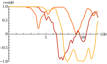
Figure 4: Illustration of typical random walks of the angle ${\cos(\phi)}$ between three pairs of test particles (with the same orbital parameters) extracted from the numerical simulations described in Appendix F. Here, we can note that the two orientations typically decorrelate after a few ${\Delta t}$, with ${\Delta t}$ defined as in Eq. (29).

To characterise this stochastic dynamics, we follow a method inspired from section 4 of Fouvry et al. (2019b), and note that the dynamics of each individual test particle can be solved formally using Magnus series (Blanes et al., 2009). One of the main advantages of such a solution is that it guarantees a good behaviour at late times. Following Eq. (29) of Fouvry et al. (2019b), the time evolution of the test particles can be solved as

$$f^{i}_{\alpha}(t)=\big{[}\mathrm{e}^{\mathbf{\Omega}_{i}(t)}\big{]}_{\alpha\delta}\,f^{i}_{\delta}(0),$$ (16)

where the sum over $\delta$ is implied. In that expression, ${\mathbf{\Omega}_{i}(t)}$ is the Magnus matrix, which to second order in the perturbative expansion reads

$$\mathbf{\Omega}_{i}(t)=-\!\!\int_{0}^{t}\!\!\!\mathbf{Q}_{i}(\tau)\,\mathrm{d}\tau+\frac{1}{2}\!\!\int_{0}^{t}\!\!\mathrm{d}\tau\!\!\int_{0}^{\tau}\!\!\!\mathrm{d}\tau^{\prime}\,\big{[}\mathbf{Q}_{i}(\tau),\mathbf{Q}_{i}(\tau^{\prime})\big{]},$$ (17)

with ${[\mathbf{A},\mathbf{B}]=\mathbf{A}\mathbf{B}-\mathbf{B}\mathbf{A}}$ the matrix commutator.

We can now use the formal solution from Eq. (16) to rewrite the correlation of the neighbours of Eq. (14) as

$$C_{\alpha\beta}(t)=\big{\langle}\big{[}\mathrm{e}^{\mathbf{\Omega}_{1}(t)}\big{]}_{\alpha\gamma}\,\big{[}\mathrm{e}^{\mathbf{\Omega}_{2}(t)}\big{]}_{\beta\delta}\big{\rangle}\,\big{\langle}f^{1}_{\gamma}(0)\,f^{2}_{\delta}(0)\big{\rangle},$$ (18)

where the sums over $\gamma$ and $\delta$ are implied, and we have solved for the time evolution of both test particles. In that expression, we assumed that the statistics of the background noise is independent of the statistics of the initial locations of the test particles. As a result, in the l.h.s. of Eq. (18), the first ensemble average is over realisations of the background, while the second average is over the initial location of the test particles.

In Appendix C, we compute the initial statistics of the test particles. In particular, we show that for isotropic initial conditions, i.e. while the location of the two test particles are correlated one with another, the distribution of any given test particle on the unit sphere is statistically uniform, the second average from Eq. (18) can generically be written as

$$\big{\langle}f^{1}_{\gamma}(0)\,f^{2}_{\delta}(0)\big{\rangle}=\frac{\delta_{\gamma\delta}}{4\pi}\,D_{\gamma},$$ (19)

In that expression, by isotropy, the diagonal matrix ${\mathbf{D}}$ sees its entries $D_{\gamma}$ only depend on $\ell_{\gamma}$. In the particular case where the two test particles are launched with the exact same initial orientations, one has ${\mathbf{D}=\mathbf{I}}$, the identity matrix.

Having characterised the test particles’ initial conditions, we can now go back to Eq. (18) which can be written as

$$C_{\alpha\beta}(t)=\big{\langle}\big{[}\mathrm{e}^{\mathbf{\Omega}_{1}(t)}\,\mathbf{D}\,\mathrm{e}^{-\mathbf{\Omega}_{2}(t)}\big{]}_{\alpha\beta}\big{\rangle},$$ (20)

where we used the fact that the matrix $\mathbf{Q}^{i}$ is skew-symmetric, i.e. ${\mathbf{Q}_{i}=-\mathbf{Q}_{i}^{\mathrm{t}}}$, so that ${[\mathrm{e}^{\mathbf{\Omega}_{i}}]^{\mathrm{t}}=\mathrm{e}^{-\mathbf{\Omega}_{i}}}$. At this stage, there are two origins to the separation undergone by the test particles: (i) their initial angular separation, as captured by the matrix $\mathbf{D}$; (ii) their difference in orbital parameters, as captured by ${\mathbf{\Omega}_{1}\neq\mathbf{\Omega}_{2}}$. The main difficulty in the computation of the ensemble average from Eq. (18) comes from the non-commutativity of the matrix exponential. This is the challenging part of the present calculation.

In Appendix D, performing a truncation at second-order in the bath fluctuations, we compute explicitly the ensemble average from Eq. (20), and obtain

$$C_{\alpha\beta}(t)=\delta_{\alpha\beta}\,D_{\alpha}\,C_{\alpha}^{\mathbf{\Omega}}(t)\,C_{\alpha}^{\mathbf{D}}(t).$$ (21)

In that expression, ${C_{\alpha}^{\mathbf{\Omega}}(t)}$ (resp. ${C_{\alpha}^{\mathbf{D}}(t)}$) captures the separation of the two test particles sourced by their differences in conserved parameters (resp. in initial orientations). They generically read

$$C_{\alpha}^{\mathbf{\Omega}}(t)=\exp\bigg{[}\frac{1}{2}\big{\langle}\big{[}\big{(}\mathbf{\Omega}_{1}-\mathbf{\Omega}_{2}\big{)}^{2}\big{]}_{\alpha\alpha}\big{\rangle}\bigg{]},$$ (22)

and

$$C_{\alpha}^{\mathbf{D}}(t)=\exp\bigg{[}\sum_{\gamma}\frac{D_{\alpha}-D_{\gamma}}{D_{\alpha}}\big{\langle}\mathbf{\Omega}^{1}_{\alpha\gamma}\,\mathbf{\Omega}^{2}_{\gamma\alpha}\big{\rangle}\bigg{]}.$$ (23)

We emphasise that Eq. (23) is symmetric w.r.t. ${(1\!\leftrightarrow\!2)}$, owing to the skew-symmetries of ${\mathbf{\Omega}^{i}}$. Having written Eqs. (22) and (23) as exponentials will guarantee a physically admissible behaviour at late times, where correlations must tend to $0$.

As detailed in Appendix D, one can push further the calculation using Eq. (8) that provides us with an explicit expression for the correlation of the bath’s fluctuations. Following this route, the associated expressions for ${C_{\alpha}^{\mathbf{\Omega}}(t)}$ and ${C_{\alpha}^{\mathbf{D}}(t)}$ are spelled out explicitly in terms of $n(\mathbf{K})$ in Eqs. (56) and (57).

These generic expressions become particularly enlightening in the limit of small initial angular separations. Assuming that the two test particles are initially separated by a small angle $\phi_{0}$, as shown in Eq. (58), one can write Eq. (21) as

$$C_{\ell}^{\mathbf{\Omega}}(t) \,=\exp\!\big{[}\!-\tfrac{1}{2}A_{\ell}\Psi^{-}(\mathbf{K}_{1},\mathbf{K}_{2},t)\big{]},$$

$$C_{\ell}^{\mathbf{D}}(t) \,=\exp\!\big{[}\!-\tfrac{1-\cos(\phi_{0})}{2}A_{\ell}\Psi^{+}(\mathbf{K}_{1},\mathbf{K}_{2},t)\big{]}.$$ (24)

In these expressions, we introduced the two auxiliary functions ${\Psi^{-}}$ and ${\Psi^{+}}$ as

$$\Psi^{-}(\mathbf{K}_{1},\mathbf{K}_{2},t) \,=\sum_{\ell}B_{\ell}\!\!\int\!\!\mathrm{d}\mathbf{K}\,n(\mathbf{K})\big{(}\mathcal{J}_{\ell}\big{[}\mathbf{K}_{1},\mathbf{K}\big{]}\!-\!\mathcal{J}_{\ell}\big{[}\mathbf{K}_{2},\mathbf{K}\big{]}\big{)}^{2}$$

$$\times \,\frac{2T_{\mathrm{c}}^{2}(\mathbf{K})}{A_{\ell}}\chi\big{[}\sqrt{A_{\ell}/2}(t/T_{\mathrm{c}}(\mathbf{K}))\big{]},$$ (25)

and

$$\Psi^{+}(\mathbf{K}_{1},\mathbf{K}_{2},t) \,=\sum_{\ell}B_{\ell}\!\!\int\!\!\mathrm{d}\mathbf{K}\,n(\mathbf{K})\mathcal{J}_{\ell}\big{[}\mathbf{K}_{1},\mathbf{K}\big{]}\mathcal{J}_{\ell}\big{[}\mathbf{K}_{2},\mathbf{K}\big{]}$$

$$\times \,\frac{2T_{\mathrm{c}}^{2}(\mathbf{K})}{A_{\ell}}(A_{\ell}\!-\!2)\,\chi\big{[}\sqrt{A_{\ell}/2}(t/T_{\mathrm{c}}(\mathbf{K}))\big{]},$$ (26)

In Eqs. (25) and (26), the only temporal dependence is in the universal dimensionless function ${\chi(\tau)}$ that reads

$$\chi(\tau) \,=\!\!\int_{0}^{\tau}\!\!\!\mathrm{d}\tau_{1}\!\!\int_{0}^{\tau}\!\!\!\mathrm{d}\tau_{2}\,\mathrm{e}^{-(\tau_{1}-\tau_{2})^{2}}$$

$$\,=\mathrm{e}^{-\tau^{2}}-1+\sqrt{\pi}\,\tau\,\mathrm{erf}(\tau).$$ (27)

This function directly stems from the double time integral of the Gaussian bath fluctuations from Eq. (8). In particular, it follows the asymptotic behaviour ${\chi(\tau)\propto\tau^{2}}$ (resp. ${\propto\tau}$) for ${\tau\ll 1}$ (resp. ${\tau\gg 1}$) which corresponds to the ballistic (resp. diffusive) part of the VRR dynamics.

Equation (24) offers a simple interpretation of the dynamical mechanisms driving the separation of neighbours. In that expression, a first source of separation stems from the different in the test particles’ parameters, as captured by the function $\Psi^{-}$ from Eq. (25). This can be seen from the coupling factor ${(\mathcal{J}_{\ell}[\mathbf{K}_{1},\mathbf{K}]\!-\!\mathcal{J}_{\ell}[\mathbf{K}_{2},\mathbf{K}])^{2}}$ in Eq. (25), which highlights that both test particles couple to the bath differently. The closer $\mathbf{K}_{1}$ and $\mathbf{K}_{2}$, the slower the separation of the particles. As expected, we recover that $C_{\alpha}^{\mathbf{\Omega}}$ becomes one in Eq. (25), when ${\mathbf{K}_{1}\!=\!\mathbf{K}_{2}}$, i.e. when the underlying annuli of the two test particles are identical.

On top of this first effect, a second source of separation originates from any initial misalignment in the test particles’ orientations. This is captured by the function $\Psi^{+}$ from Eq. (26), which does not vanish even when the two test particles have the same orbital parameters. In addition, as highlighted in Eq. (24), the smaller the initial separation of the two test particles, i.e. the smaller ${(1\!-\!\cos(\phi_{0}))}$, the longer it takes for the neighbours to get separated. In particular, we note that ${C_{\ell}^{\mathbf{D}}}$ becomes one when ${\cos(\phi_{0})\to 1}$, i.e. when the two test particles share the exact same initial orientation. Note that Eq. (26) involves an extra ${(A_{\ell}\!-\!2)\!=\!(\ell(\ell\!+\!1)\!-\!2)}$ which corresponds to a Laplacian, reflecting the fact that pair separations are only sensitive to tides, not forces. Moreover, should the harmonics ${\ell=1}$ have been able to drive the VRR dynamics, this particular harmonics would not have been able to drive any neighbour separation through orientations mismatches, as highlighted by the vanishing factor ${A_{\ell=1}\!-\!2\!=\!0}$ in Eq. (26).

Let us further note that the prediction from Eq. (24) is self-similar, i.e. the only dependence on the considered harmonics $\ell$ is carried by ${A_{\ell}}$, which is factored in the exponent. For a given pair of test stars (that is, fixing the shape of $\Psi^{+}$), the prediction from Eq. (24) only depends on the product ${A_{\ell}(1\!-\!\cos(\phi_{0}))}$. Since ${1/\sqrt{A_{\ell}}}$ is the characteristic scale of the $\ell^{\mathrm{th}}$ harmonics, this product compares the test particles’ separation with that of the considered harmonics. In particular, on the one hand, harmonics whose scale is larger than the particles’ separation, i.e. such that ${A_{\ell}(1\!-\!\cos(\phi_{0}))\ll 1}$ do not decorrelate efficiently. This is because the potential generated by these bath harmonics is roughly constant on the scale of the particles’ separation. We note that even for these large scale harmonics, there is still an unavoidable separation stemming from the non-vanishing contribution of $C_{\ell}^{\mathbf{\Omega}}$, which, in that limit, captures the effect of phase mixing, i.e. the frequency shearing of test particles with different orbital parameters. On the other hand, higher order harmonics, i.e. such that ${A_{\ell}(1\!-\!\cos(\phi_{0}))\gtrsim 1}$, are much more efficient at driving neighbour separation since they vary on angular scales similar to or smaller than the initial separation of the test particles.

Finally, we emphasise that both functions $\Psi^{-}$ and $\Psi^{+}$ only depend on the test particles’ parameters, $\mathbf{K}_{1}$ and $\mathbf{K}_{2}$, as well as on the background cluster’s parameters, ${n(\mathbf{K})}$. As highlighted in Eq. (24), these functions are independent of the harmonics $\ell$ of the considered correlation function, as well as of the statistics of the test particles’ initial separation, given by ${\cos(\phi_{0})}$. These functions will prove very useful in Section 4 to construct our piecewise prediction.

Equations (21) and (24) are the main results of this section. In practice, one is not limited to only considering two test particles, but can rather consider an arbitrary population of test particles that follow initially a given smooth distribution. It is straightforward to expand Eq. (21) to such a population, as detailed in Appendix E. In short, one has

$$\big{\langle}f_{\alpha}(\mathbf{K},t)\,f_{\beta}(\mathbf{K}^{\prime},t)\big{\rangle}\simeq p(\mathbf{K})\,p(\mathbf{K}^{\prime})\,C_{\alpha\beta}(\mathbf{K},\mathbf{K}^{\prime},t),$$ (28)

where ${p(\mathbf{K})}$ is the PDF of the orbital parameters of the test particles and $C_{\alpha\beta}(\mathbf{K},\mathbf{K}^{\prime},t)$ is given by Eq. (21), assuming that the orbital parameters of the two test particles are resp. $\mathbf{K}$ and $\mathbf{K}^{\prime}$.

Let us emphasise once again the generality of Eq. (21) that captures jointly three physical contributions modulating the efficiency of the neighbours separation: (i) the orbital distribution of the background particles, via ${n(\mathbf{K})}$; (ii) the orbital differences of the two test particles, via $\mathbf{K}_{1}$ and $\mathbf{K}_{2}$, and further through the PDF ${p(\mathbf{K})}$ appearing in Eq. (28); (iii) the difference in the initial orientation, via $\mathbf{D}$. In all these expressions, time is measured in units of ${T_{\mathrm{c}}(\mathbf{K})}$, the coherence time of the bath’s fluctuations, which defines the typical timescale for that process. As such, Eq. (21) is a very general result, that can be applied to a wide variety of physical processes. For instance, in Section 5 we will use it to put constraints on ${n(\mathbf{K})}$, which describes the unresolved old stellar cluster.

We may now test the predictions of Eq. (21) against some tailored numerical simulations. These simulations are similar to those of Fouvry et al. (2019b), and we detail our exact setup in Appendix F. Our main result is illustrated in Fig. 5.

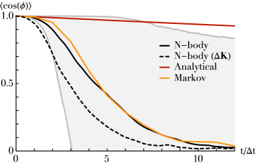
Figure 5: Correlation of the separation of a population of test particles with the same orbital parameters, as measured in numerical simulations (see Appendix F for details) and predicted by Eq. (21). Here, the timescale ${\Delta t}$ was chosen following Eq. (29). The ‘Analytical’ prediction corresponds to the direct application of Eq. (21), while the ‘Markov’ prediction corresponds to the improved prediction following the approach from Appendix I. Because of the very slow separation of nearby particles, the prediction from Eq. (21) does not provide a good match to the late-time decorrelation of test particles that start with very similar initial orientations. Finally, the curve ‘${\Delta\mathbf{K}}$’ illustrates the correlation measured in numerical simulations where the test particles do not share the exact same orbital parameters, which further accelerates their dilution.

Here, we compare the measurements of particle’s dilution in numerical simulations with the analytical predictions from Eq. (21). First, in that figure, we represented two numerical measurements of correlations, depending on whether or not the test particles also differ in their conserved orbital parameters. As expected, the separation in parameters, as captured by the term $C_{\alpha}^{\mathbf{\Omega}}$ from Eq. (21), contributes to further accelerating the particles’ separation. Unfortunately, in Fig. 5, we note that the ‘Analytical’ prediction, i.e. the prediction from Eq. (21), does not manage to accurately capture the late-time decay of the particles’ separation. However, we do note that on the coherence time, i.e. for ${t\lesssim\Delta t}$ (see the definition of ${\Delta t}$ in Eq. (29)), the analytical prediction indeed matches the numerical measurements. This is expected from the fact that the prediction from Eq. (21) was obtained through a Taylor series around ${t=0}$. Yet, in its present form, the prediction from Eq. (21) is not able to describe the unavoidable separation of the test particles sharing very similar orientations and orbital parameters, as this prediction follows a plateau that only decays on very long timescales. Fortunately, this apparent failure of the analytical prediction can be alleviated by using an appropriate Markovian approach, leading to the improved ‘Markov’ prediction in Fig. 5, that quantitatively matches with the numerical measurements. This is what we explore in the next section.

4 Piecewise Markovian prediction

The results from the previous section, in particular Figure 5, show that the straight application of the theoretical prediction from Eq. (21) is not enough to compute the rate of separation of the test particles when they are too similar, i.e. when both their initial orientations and their conserved orbital parameters are very similar. In these cases, the correlations measured in the $N$-body simulations present a plateau in ${t\!=\!0}$. This suggests that the perturbative expansion used to obtain Eq. (21) might not contain enough information about the dynamics to accurately model the particles’ separation. Our goal is now to show how one can improve the analytical prediction from Eq. (21) so that it could also apply to cases where the separation of the neighbours is very slow.

In practice, in Appendix D we performed a second-order Taylor expansion, so that the analytical prediction from Eq. (21) only matches the first two derivatives at ${t\!=\!0}$ of the numerically measured correlation. As soon as a plateau appears in Fig. 5, i.e. as soon as the contribution from the first derivatives is small compared to the contribution of higher-order derivatives, this perturbative development breaks down. This happens in particular when the two test particles share very similar orientations. Indeed, since the potential field generated by the background bath is large-scale and continuous, the two neighbours feel a very similar potential, and as such need a lot of time (compared to $T_{\mathrm{c}}$, the coherence time of the noise) to separate one from another.

Fortunately, regardless of the initial similarity between the test particles, Eq. (21) works well for short timescales, that is when ${t\lesssim T_{\mathrm{c}}(\mathbf{K})}$. As a result, a reasonable way of fixing the late-time behaviour of our prediction is to construct a sequence of short-time predictions, following for each of them Eq. (21). Let us therefore pick a timelapse ${\Delta t}$ (whose precise value will be picked later on), and construct a piecewise prediction of ${\langle\cos(\phi)\rangle}$, splitting the prediction from Eq. (21) in timelapses of duration ${\Delta t}$. Doing so, we therefore construct a sequence ${\cos(\phi_{0}),...,\cos(\phi_{n})\!=\!\cos(\phi(t\!=\!n\Delta t))}$ of angular separations between the two test particles. In order to construct the prediction for a given timelapse, say ${n\Delta t\to(n+1)\Delta t}$, we follow Eq. (21), and use ${\cos(\phi_{n})}$ as the initial angular separation between the two test particles and ${t=\Delta t}$ as the time duration during which Eq. (21) is pushed forward in time.

Such a piecewise protocol is not equivalent to making a single prediction for the whole time series using only ${\cos(\phi_{0})}$ as the initial separation in Eq. (21). Indeed, there are two main differences with the present piecewise approach. First, when making the analytical prediction in Fig. 5, the only angular information used in the equations was the statistics of the initial angular separation, ${\cos(\phi_{0})}$. Here, the current value of the angular separation, ${\cos(\phi_{n})}$, is used at the start of each timelapse of duration ${\Delta t}$. Second, because the current angular separation, ${\cos(\phi_{n})}$, is now used in Eq. (21) as an initial condition of the $n^{\mathrm{th}}$ timelapse, the piecewise approach neglects any correlation that might exist in the background noise between the various timesteps. Indeed, when deriving the prediction from Eq. (21), we had to assume that the initial conditions of the test particles are independent from the state and statistics of the background bath (as highlighted in Eq. (18)). In the present piecewise case, since we proceed by successive timesteps, we neglect any such correlations. This is our Markovian assumption, a key ingredient of the piecewise prediction.

Hence the ideas behind this piecewise approach are very similar to the explicit Euler method used to solve differential equations. Rather than limiting ourselves to approximating the solution with a single perturbative expansion around its initial conditions, we construct the solution of Eq. (13) step by step. There is however one difference with traditional step-by-step methods, which is the fact that Eq. (13) is stochastic, so that the noise driving the separation of neighbours is time-correlated. As a result, by proceeding by successive timelapses, we unavoidably neglect some part of that correlation. As such, if we were to take ${\Delta t}$ arbitrarily small, as is usually done in non-stochastic cases to increase their accuracy, we would be actually replacing the VRR fluctuations by a noise uncorrelated in time. In that limit, the reconstructed motion would be Brownian, which drastically differs from the large scale gravitationally-driven motion imposed by VRR.

The choices for ${\Delta t}$ are therefore limited. One the one hand, in order to capture most of the noise correlation, one needs ${\Delta t\gtrsim T_{\mathrm{c}}}$, with $T_{\mathrm{c}}$ (see Eq. (9)) an estimate of the noise coherence time. On the other hand, in order for each of the timelapses to be accurately predicted, one needs to take ${\Delta t}$ as small as possible. Given these two constraints, a natural choice is to take ${\Delta t}$ of the order of $T_{\mathrm{c}}$.

In practice, one can note from Eq. (8) that the coherence time of the noise generated by the bath, ${T_{\mathrm{c}}(\mathbf{K})}$, depends both on $\mathbf{K}$ (i.e. the bath has a whole range of decorrelation timescales), as well as on $\ell$ (i.e. different harmonics separate neighbours on different physical scales). For two test particles having identical orbital parameters, $\mathbf{K}$, we choose to define the timestep ${\Delta t}$ as

$$\Delta t=T_{\mathrm{c}}(\mathbf{K}).$$ (29)

Here, returning to Eq. (8), we note that the ${\ell=2}$ harmonics of the noise, which has the longest correlation time and the largest scale correlation length, decays on a timescale of the order ${\sqrt{2/A_{2}}T_{\mathrm{c}}\!=\!T_{\mathrm{c}}/\sqrt{3}}$, which justifies our choice for ${\Delta t}$. Furthermore, in Eq. (29), we chose to evaluate the coherence time for the orbital parameters $\mathbf{K}$, following the observation that test particles mainly interact with bath particles that have similar parameters, as can be seen in the dependence of the coupling coefficients, ${\mathcal{J}_{\ell}[\mathbf{K},\mathbf{K}^{\prime}]}$, in Fig. 10. In the general case where the two test particles do not share the same orbital parameters, i.e. ${\mathbf{K}_{1}\neq\mathbf{K}_{2}}$, we opt for the most conservative choice. We therefore take the maximum of ${\Delta t}$ obtained for both particles.

When considering a population of more than two test particles, we have shown in Eq. (28) that the dilution is given by the average of the two-point correlation functions of pairs of neighbours. As a consequence, to apply the piecewise approach to a population of test particles, one only has to deal with each pair of neighbour separately, and then average over them. Note that, following Eq. (29) different timesteps ${\Delta t}$ can be used for each pair of test particles. Since the coherence time $T_{\mathrm{c}}$ can vary substantially between pairs of particles, this allows for the use of a somewhat optimal timestep for each pair.

4.1 Direct evolution of the correlation

Having decided upon a timestep ${\Delta t}$ in Eq. (29), let us now apply the previous piecewise protocol to find a better estimate of the separations measured in Fig. 5. Since our goal is to construct typical sequences ${\cos(\phi_{0})\rightarrow...\rightarrow\cos(\phi_{n})}$ of angular separations between two neighbours, we must estimate the statistics of the transition from one angle to the following, i.e. the statistics of the transition ${\cos(\phi_{i})\rightarrow\cos(\phi_{i+1})}$. Of course, these transitions are stochastic so that the separations ${\cos(\phi_{i})}$ are themselves random variables that depend on the realisations of the background noise. Specifically we aim to compute the average properties of these separations, and, as in Fig. (5), predict ${\langle\cos(\phi)\rangle}$.

We therefore need to compute the expectation of ${\cos(\phi_{i+1})}$ conditionally to the value of ${\cos(\phi_{i})}$. Indeed, within the Markovian approximation, it is only the angular separation of the test particles at the start of a given timelapse, i.e. ${\cos(\phi_{i})}$, that matters for its subsequent evolution during that same timestep. As a result, we can naturally write

$$\langle\cos(\!\phi_{i+1}\!)\rangle\!=\!\!\int\!\!\mathrm{d}(\cos(\!\phi_{i}\!))\,\rho_{i}(\cos(\!\phi_{i}\!))\langle\cos(\!\phi_{i+1}\!)|\cos(\!\phi_{i})\rangle,$$ (30)

In that expression, ${\langle\cos(\phi_{i+1})|\cos(\phi_{i})\rangle}$ follows from Eq. (21), evaluated after a time ${t=\Delta t}$ for two test particles systematically separated by the constant angle ${\cos(\phi_{i})}$ at the start of the timelapse (see Eq. (43) for the associated coefficients ${D_{\ell}}$). In Eq. (30), we also formally introduced ${\rho_{i}}$ as the PDF of ${\cos(\phi_{i})}$. In practice, that PDF is not known, so that without further approximation, the integral from Eq. (30) cannot be explicitly computed.

The simplest way around is to rely on a first-order development of ${\langle\cos(\phi_{i+1})|\cos(\phi_{i})\rangle}$ near ${\cos(\phi_{i})\simeq 1}$, i.e. in the limit of small angular separations. As detailed in Appendix G, in that limit one obtains a linear relationship between the initial condition ${\cos(\phi_{i})}$ and the conditional expectation ${\langle\cos(\phi_{i+1})|\cos(\phi_{i})\rangle}$, reading

$$\langle\cos(\phi_{i+1})|\cos(\phi_{i})\rangle=\xi_{0}+\xi_{1}\cos(\phi_{i}).$$ (31)

The coefficients $\xi_{k}$ follow from the prediction of Eq. (21), and their detailed values are given in Eq. (71). In particular, we emphasise that these coefficients are independent of the test particles’ current angular separation, and depend only on their orbital parameters, $\mathbf{K}_{1}$ and $\mathbf{K}_{2}$, as well as on the background’s DF, ${n(\mathbf{K})}$.

Following Eq. (30), let us now compute the average of Eq. (31) to obtain

$$\langle\cos(\phi_{i+1})\rangle=\xi_{0}+\xi_{1}\,\langle\cos(\phi_{i})\rangle.$$ (32)

This is the key relation of the piecewise approach, as we have been able to obtain a relation between the successive values ${\langle\cos(\phi_{i})\rangle}$ and ${\langle\cos(\phi_{i+1})\rangle}$. Equation (32) is an arithmetic-geometric relation. As a consequence, given an initial condition ${\langle\cos(\phi_{0})\rangle}$, it uniquely defines a sequence of expectations for all the subsequent timesteps, ${t=i\Delta t,\,i\geq 0}$. We refer to Eq. (72) for the explicit solution of Eq. (32). This is our piecewise prediction.

In Fig. 6, we compare the piecewise prediction from Eq. (32) against the numerical measurements from Fig. 5.

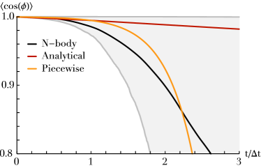
Figure 6: Initial correlation of the separation of a population of test particles with the same orbital parameters, using the exact same numerical simulations as in Fig. 5. The ‘Analytical’ prediction corresponds to the direct application of Eq. (21), while the ‘Piecewise’ prediction corresponds to the use of the piecewise Markovian approach of Eq. (32). This second prediction is able to describe the slow initial separation of the particles and, as a result, matches the numerical measurements much better.

While the match between the numerical measurements and the piecewise prediction is not ideal, the piecewise prediction presented in Fig. 6, can describe the first stages of (slow) separation of the test particles, while the straightforward application of the analytical prediction from Eq. (21) failed at it.

In practice, the perturbative expansion performed in Eq. (31) is only valid for small angular separations. As a consequence, a piecewise sequence generated with the protocol from Eq. (32) will only match the numerical measurements as long as the test particles remain sufficiently close to one another. This is, however, not a problem since these first steps of (very) slow initial separation are the hardest ones to predict, as already illustrated in Fig. 5. Indeed, once ${\langle\cos(\phi_{i})\rangle}$ has slightly decreased, i.e. once the test particles have been slightly stirred away from one another through the VRR fluctuations, a straightforward use of Eq. (21) would be enough to predict the rest of the time series. This would allow us to extend our prediction for the separation to arbitrarily large times. In practice, we find that the piecewise prediction behaves properly for ${\langle\cos(\phi)\rangle\gtrsim 0.8}$, i.e.  ${\phi\lesssim 37^{\circ}}$. This is enough for most astrophysical applications, e.g., the possible dilution of SgrA*’s clockwise stellar disc whose typical angular separation is ${16^{\circ}}$ (Gillessen et al., 2017).

Following Eq. (32), determining the timescale associated with the dilution of an initial patch of test particles then only amounts to computing once the two coefficients, $\xi_{k}$, and determining at which time ${\langle\cos(\phi)\rangle}$ gets below a given threshold, e.g., 0.95. Since this is such a simple calculation, it can then be used to very efficiently explore the parameters of the test particle’s distribution. This is illustrated in Fig. 7, where we show how the efficiency of the dilution varies as one changes the initial angular separation of the test particles or their conserved orbital parameters.

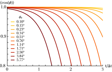
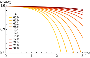
Figure 7: Illustration of the rate of neighbour separation as predicted by the piecewise approach from Eq. (32). Here, the background bath follows the same statistics as in Fig. 6, while the test particles share the same orbital parameters, ${(a,e)\simeq(10,0.21)}$. Top panel: Correlation of the separation as one varies the initial angle $\phi_{0}$ between the particles. The closer the two particles, the slower the dilution. Bottom panel: Same correlations for test particles initially separated by ${\phi_{0}=3^{\circ}}$, as one varies their shared semi-major axis, $a$. In that panel, the rescaled time was picked for the smallest ${\Delta t(a\!=\!5)}$. The larger $a$, the slower the dilution.

As expected, the smaller the initial patch, the slower the separation. Similarly, the larger the semi-major axes of the test particles, the larger their $T_{\mathrm{c}}$ (see Eq. (9)), and therefore the slower their dilution. In Section 5, we will further illustrate the versatility of this approach by presenting some first applications of Eq. (32) to estimate the efficiency of the dilution of the clockwise disc surrounding SgrA*.

As highlighted in Eq. (32), the piecewise prediction can only predict the expectation of ${\langle\cos(\phi)\rangle}$ throughout the dilution of the test particles. It cannot predict higher order moments of ${\langle\cos(\phi)\rangle}$, nor can it be used to produce effective random walks of the stochastic variable ${\cos(\phi)}$. Relying on the use of a restricted ${\ell=2}$ toy model (see Appendix H), this is what we explore in Appendix I to generate virtual dilutions. It is this particular approach that was used in Fig. 5 to produce a Markovian prediction that matches the numerical measurements even at late times.

5 Application: cusp properties from dilution

Let us now consider a background stellar cusp distribution similar to SgrA*’s. We will now show how our results allow us to probe the underlying kinematic properties of the unresolved nucleus when requesting consistency with level of neighbours dilutions. We will not aim to be very realistic nor match any specific data, as this will be the topic of an upcoming investigation.

Following Gillessen et al. (2017), we take the mass of the central BH to be ${M_{\bullet}=4.3\!\times\!10^{6}M_{\odot}}$. For simplicity, we first assume that the background old stellar cluster is made of a single-mass stellar population of individual mass ${m_{\star}=1M_{\odot}}$. We assume that the stars’ eccentricities follow a thermal distribution, ${f_{e}(e)=2e}$ (Merritt, 2013), and that the number of stars per unit $a$ follows a power-law distribution of the form ${n_{a}(a)\propto a^{2-\gamma}}$. The detailed normalisations for that setup are all summarised in Appendix J. In such a configuration, Fouvry et al. (2019b) (see Eq. (48) therein) have shown that the coherence time of the fluctuations, ${T_{\mathrm{c}}(\mathbf{K})}$ (see Eq. (9)), follows the simple dependence

$$T_{\mathrm{c}}(a,e)\simeq 1.4\!\times\!\frac{P(a)}{\sqrt{N(\!<\!a)}}\,\frac{M_{\bullet}}{\sqrt{\langle m^{2}\rangle}}\,\sqrt{1\!-\!e^{2}},$$ (33)

where ${P(a)\!=\!2\pi(a^{3}/(GM_{\bullet}))^{1/2}}$ is the (fast) Keplerian period, ${N(\!<\!a)\!\propto\!a^{3-\gamma}}$ is the number of stars physically within a sphere of radius $a$ from the centre, and ${\sqrt{\langle m^{2}\rangle}}$ captures the mass spectrum of the background cluster. In particular, the larger the spread in mass, the larger the eccentricity, the lighter the central black hole, the shorter the coherence time. Equation (33) will prove useful to interpret some of the trends of the upcoming figures.

We now consider a population of test particles mimicking the stars belonging to the clockwise disc (Gillessen et al., 2017). To simplify, we assume that all the test stars share the same orbital parameters, so that we take, as an example, ${a_{\mathrm{t}}=50\,\mathrm{mpc}}$ and ${e_{\mathrm{t}}=0.1}$. As such, we are not accounting for any separation stemming from differences in the test particles’ orbital parameters, see Eq. (25), which would further reduce the timescales predicted here. We assume that the test stars are born with an average angular separation given by ${\langle\cos(\phi_{0})\rangle}$, and that their age are somewhat similar to those of the inner S-stars (Habibi et al., 2017), so that ${t_{\star}\simeq 10\,\mathrm{Myr}}$. Having specified the parameters of the disc’s stars, the prediction from Eq. (21) (in particular its piecewise version from Eq. (32)) can be used to estimate the typical time required for such a stellar disc to dilute. Following Gillessen et al. (2017), the current angular dispersion of the clockwise disc is approximately given by ${\langle\phi_{\mathrm{disc}}\rangle\simeq 16^{\circ}}$, This corresponds to an average separation ${\langle\cos(\phi_{\mathrm{disc}})\rangle\simeq 0.96}$, which is well within the regime of applicability of the piecewise prediction, see Fig. 6. For a given model of the background cluster and a given initial condition, we then define the diffusion time, $T_{\mathrm{diff}}$, as the time required for ${\langle\cos(\phi)\rangle}$ to reach ${\langle\cos(\phi_{\mathrm{disc}})\rangle}$. Once the average angular separation between the test stars has reached such a large value, one may consider that the stellar disc has been effectively dissolved by the VRR fluctuations.

Figure 8 illustrates the variations of the dilution time as one varies the power index of the background stellar cusp, ${\gamma_{\star}}$, as well as the initial angular dispersion, ${\langle\cos(\phi_{0})\rangle}$.

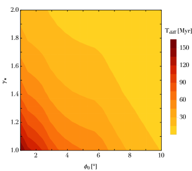
Figure 8: Illustration of the dependence of the dilution time, $T_{\mathrm{diff}}$, of the stellar disc, as a function of the disc’s initial angular separation, $\phi_{0}$, and the cusp index of the background stellar cluster. Light colours correspond to fast dilution times. In particular, we recover that the larger the initial angular dispersion and the larger the cusp index, the faster the dilution.

As already highlighted in Fig. 7, the smaller the initial patch of stars, the longer it takes for the initially coherent stellar disc to dissolve. Figure 8 also shows that the cuspier the density profile, the faster the dilution. This dependence is a direct consequence of the factor ${1/\sqrt{N(\!<\!a)}}$ in the expression of ${T_{\mathrm{c}}(\mathbf{K})}$ from Eq. (33): the larger $\gamma_{\star}$, the larger ${N(\!<\!a)}$, therefore the smaller the coherence time, ${T_{\mathrm{c}}(\mathbf{K})}$, and hence the faster the dilution of the disc. While the numerical values used here are in some sense ad hoc, and would definitely require more careful selections, Fig. 8 shows how the present formalism could be used to place constraints on the parameters of the unresolved background stellar cluster (here through its index $\gamma_{\star}$) as well as on the formation channels of stars in galactic nuclei (here through the size of their initial angular patch $\phi_{0}$).

Let us finally assume that the background cluster is composed not only of old stars, but also of intermediary mass black holes. For simplicity, let us assume that the total enclosed mass remains the same, and that the IMBHs follow the same ${(a,e)}$ distribution than the stars, with an individual mass given by ${m_{\bullet}=100\,M_{\odot}}$. The details of our normalisation are given in Appendix J. In the top panel of Fig. 9, we illustrate the dependence of the dilution time as one varies the mass fraction of the IMBHs, as well as their shared power index, $\gamma$.

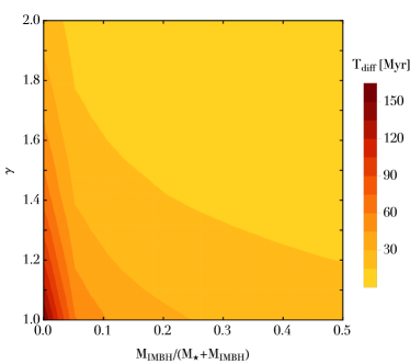
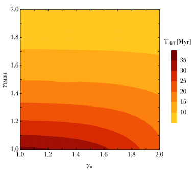
Figure 9: Illustration of the dependence of the dilution time, $T_{\mathrm{diff}}$, of the stellar disc, when the background cluster also contains some IMBHs, assuming an initial angular separation given by ${\phi_{0}=3^{\circ}}$. Top panel: As a function of the IMBHs’ mass fraction and their shared cusp index. Bottom panel: As a function of the old stars’ and IMBHs’ cusp indices, assuming an IMBH mass fraction of ${M_{\mathrm{IMBH}}/(M_{\mathrm{IMBH}}\!+\!M_{\star})\!=\!20\%}$. As expected, the higher the fraction of IMBHs, and the higher the cusps’ indices, the faster the dilution of the stellar disc.

As expected, one recovers that a larger fraction of IMBHs leads to a faster dilution of the disc stars. This is a direct consequence of the factor ${1/\sqrt{\langle m^{2}\rangle}}$ present in Eq. (33): the larger the fraction of IMBHs, the larger ${\langle m^{2}\rangle}$, and therefore the smaller ${T_{\mathrm{c}}(\mathbf{K})}$. In practice, this acceleration of the dilution through the mass spectrum is slightly dampened by the factor ${1/\sqrt{N(\!<\!a)}}$ from Eq. (33) which increases when the mass fraction of IMBHs increases as the total number of background particles decreases overall.

In practice, within the old unresolved stellar cluster, NR has had the time to lead to mass segregation, so that one expects that the old stars and the IMBHs not to share the same power index, the heavier particles being on more cuspy distributions (Bahcall & Wolf, 1977). This is briefly explored in the bottom panel of Fig. 9, where for a fixed mass fraction in IMBHs, we explore the dependence of the dilution time as one varies independently the power indices of both populations. In that figure, we recover that cuspier profiles lead to more efficient separations, the effect being most visible for the IMBH’s population.

All in all, even though the typical timescale of VRR is given by $T_{\mathrm{c}}$, Figs. 8 and 9 show that the timescale for particle separation can be significantly longer than $T_{\mathrm{c}}$. For the range of parameters explored here, we approximately find

$$\frac{T_{\mathrm{diff}}}{T_{\mathrm{c}}}\simeq 1\,\hbox{---}\,15,$$ (34)

depending mainly on the disc’s initial angular dispersion.

Of course, the explorations from Figs. 8 and 9 are only preliminary applications in the context of SgrA*. In particular, here we only focused on the dynamical constraint associated with the observation of the clockwise disc on the scale ${a\simeq 50\,\mathrm{mpc}}$. But a dual constraint also comes from the fact that in more internal regions, ${a\simeq 5\mathrm{mpc}}$, the observed S-cluster has a seemingly isotropic distribution of orientations. As such, to be physically admissible any model for SgrA*’s cluster must ensure both a fast enough dilution time of stellar discs in its center, and a slow enough dilution time further out. These joint constraints will eventually allow us to bracket the physical parameters of the cluster.

6 Conclusions

This paper illustrated how to quantitatively describe the two-point statistical properties of neighbour separation induced by vector resonant relaxation. Section 2 assumed the limit of an isotropic distribution of background stars, whose potential fluctuations slowly stir neighbour particles away from one another. A key result was obtained in Eq. (21), which highlighted the two main effects sourcing the separation of nearby particles, namely their difference in orientations and their differences in conserved orbital parameters. Relying on a Markovian assumption, this estimator was subsequently improved in Section 4 and Appendix I through the construction of both a piecewise prediction and generations of virtual realisations. This approach allowed us in particular to describe the (very) slow separation of highly correlated neighbour stars, e.g., test particles starting with very close orientations. Throughout the text, all our predictions were compared with tailored numerical simulations, which led to a quantitative agreement on the rate of neighbour separation. Finally, Section 5 presented a first application of this formalism to determine the efficiency with which young stellar discs, such as the one observed within SgrA*, can spontaneously dissolve under the effects of the stochastic VRR dynamics. In particular, we showed how the initial distribution of angular separation of the disc, the profile of the background unresolved cluster, as well as the possible presence of IMBHs all influence the efficiency with which discs spontaneously dissolve in galactic nuclei.

This paper only addresses some aspect of what a complete theory of VRR should achieve. Here is a list possible avenues for future development.

First, the toy model for SgrA* presented in Section 5 is only a preliminary validation and illustration of the computation of the dissolution time of SgrA*’s clockwise disc. Indeed, two observational constraints must be satisfied by any model of the underlying background stellar cluster: (i) the most inner S-stars seem to have an isotropic distribution of orientations, while (ii) some of the outer stars seem to belong to a disc-like structure (Gillessen et al., 2017). As a consequence, the separation of neighbours sourced by VRR must be on the one hand efficient enough to mix the inner stars, and on the other hand inefficient enough to allow for the outer disc to survive up to the present time. Using jointly these observational requirements, one should therefore be in a position to place constraints on the properties of the underlying stellar cluster (e.g., possible existence of IMBHs) and of the formation mechanism of the S-stars (e.g., through an episode of star formation in a disc). Such detailed explorations of parameter space are made possible by the present formalism because it allows very easily for variations in the bath’s DF (via ${n(\mathbf{K})}$), the test particles’ DF (via ${p(\mathbf{K})}$), as well as their initial separation (via ${\langle\phi_{0}\rangle}$). This will be the subject of a future work.

The present framework relied extensively on the isotropic assumption, both for the background potential fluctuations, but also for the test particles’ initial conditions. As a result, any effects associated with possible anisotropic clusterings in orientation (Szölgyén & Kocsis, 2018) was neglected. Indeed, such non-spherical structures stemming from the VRR long-term thermodynamical equilibria can undoubtedly affect the statistical properties of the fluctuations in the system (in particular for the most massive background particles), and as a result may also change the efficiency of neighbour separation.

Here, the limit of test particles was assumed, so that any self-gravity among neighbouring particles was neglected. This assumption is only (reasonably) valid in the limit where these pairwise interactions are indeed negligible in front of the bulk of interactions sourced by the background stellar cluster. In practice, owing to the sharpness of the coupling coefficients, $\mathcal{J}_{\ell}$, see Fig. 10, a given star mainly interacts with stars that share similar parameters (in particular semi-major axes), and similar orientations. All in all, this tends to enhance the gravitational coupling between two neighbour particles, making our present assumption of test particles less valid. For example, the importance of self-gravity among the particles from the same disc was already highlighted in Figs. 6 and 7 of Kocsis & Tremaine (2011), where one notes that self-gravity increases the coherence of the disc, and reduces the efficiency with which it can dissolve. Accounting for this self-gravitating component is no easy task, and definitely deserves further theoretical investigations.

The present analysis focused on an isotropic description of the dilution process. Strikingly, simulations such as those shown in Fig. 2 suggest that this process is significantly non-isotropic, with a clear elongation of the tracer distribution. It would therefore be interesting to quantify, e.g., through the three-point correlation function, the rate at which these elongation arise. This could then be used as a supplementary observational constraint to leverage all the information coming from future observations of SgrA* (Do et al., 2019). Similarly, it could also prove useful to further expand the analytical calculations from Appendix D to compute the theoretical predictions up to fourth-order in the fluctuations. This could be of importance in particular to better describe very slow separations, to improve the quality of the piecewise predictions, or to be able to generate virtual dilutions also in the case of test particles with different orbital parameters.

Finally, this paper focused on systems dominated by a central mass. But, as long as one updates accordingly the coupling coefficients, ${\mathcal{J}_{\ell}}$, the same VRR process also happens in globular clusters (Meiron & Kocsis, 2018). In that context, one could investigate the efficiency of the mixing (in orientations) of neighbouring stars. In the light of the exquisite GAIA data, this dynamical process could prove important to understand how co-eval stars can mix in the crowded stellar environments of globular clusters.

Appendix A Coupling coefficients

Let us detail the expression of the coupling coefficients, ${\mathcal{J}_{\ell}\big{[}\mathbf{K}_{i},\mathbf{K}_{j}\big{]}}$, that characterise the strength of the pairwise VRR interaction in the Hamiltonian from Eq. (2). Following Eq. (51) of Fouvry et al. (2019b), they stem from the multipole expansion of the Newtonian interaction and read

$$\mathcal{J}_{\ell}\big{[}\mathbf{K}_{i},\mathbf{K}_{j}\big{]}\!=\!\frac{Gm_{i}m_{j}}{L(\mathbf{K}_{i})}\frac{4\pi P_{\ell}^{2}(0)}{2\ell+1}\!\!\int_{0}^{\pi}\!\!\!\frac{\mathrm{d}M_{i}}{\pi}\!\!\int_{0}^{\pi}\!\!\!\frac{\mathrm{d}M_{j}}{\pi}\,\frac{\mathrm{Min}[r_{i},r_{j}]^{\ell}}{\mathrm{Max}[r_{i},r_{j}]^{\ell+1}},$$ (35)

with ${L(\mathbf{K})=m\sqrt{GM_{\bullet}a(1\!-\!e^{2})}}$ the norm of the angular momentum. Note the presence of the Legendre polynomials, ${P_{\ell}(0)}$, which ensures that these coefficients are non-zero only for even values of $\ell$. Finally, in Eq. (35) we introduced $M$ as the mean anomaly associated with a given Keplerian orbit. This equation already shows that more radial orbits (${e\simeq 1}$) will have larger $\mathcal{J}_{\ell}$, since they have smaller angular momentum $L$. As a result, they are more easily reoriented.

In order to highlight the scale-invariance of these coupling coefficients, let us rewrite the orbit-average integral as an integral over eccentric anomalies, that we denote with $\phi$. To do so, we also introduce ‘$\mathrm{out}$’ (resp. ‘$\mathrm{in}$’) as the index $i$ or $j$ with the larger (resp. smaller) semi-major axis, and introduce the ratio ${\alpha=a_{\mathrm{in}}/a_{\mathrm{out}}\leq 1}$. Given the relation ${\mathrm{d}M/\mathrm{d}\phi=r/a}$, and the explicit expression of the radius ${r\!=\!a(1\!-\!e\cos(\phi))}$, Eq. (35) finally reads

$$\mathcal{J}_{\ell}\big{[}\mathbf{K}_{i},\mathbf{K}_{j}\big{]}=\frac{Gm_{i}m_{j}}{a_{\mathrm{out}}}\frac{1}{L(\mathbf{K}_{i})}\,s_{\ell}\big{[}\alpha,e_{\mathrm{in}},e_{\mathrm{out}}\big{]},$$ (36)

where the dimensionless coefficients ${s_{\ell}\big{[}\alpha,e_{\mathrm{in}},e_{\mathrm{out}}\big{]}}$ read

$$s_{\ell}\big{[}\alpha,e_{\mathrm{in}}, \,e_{\mathrm{out}}\big{]}=\frac{4\pi P_{\ell}^{2}(0)}{2\ell+1}\,\frac{1}{\alpha}\!\!\int_{0}^{\pi}\!\!\frac{\mathrm{d}\phi}{\pi}\!\!\int_{0}^{\pi}\!\!\frac{\mathrm{d}\phi^{\prime}}{\pi}$$

$$\times \,\frac{\mathrm{Min}\big{[}\alpha(1\!-\!e_{\mathrm{in}}\cos(\phi)),(1\!-\!e_{\mathrm{out}}\cos(\phi^{\prime}))\big{]}^{\ell+1}}{\mathrm{Max}\big{[}\alpha(1\!-\!e_{\mathrm{in}}\cos(\phi)),(1\!-\!e_{\mathrm{out}}\cos(\phi^{\prime}))\big{]}^{\ell}}.$$ (37)

Such a dimensionless writing is an appropriate form to deal with infinite power-law distributions as in Section 5.

Figure 10 illustrates the typical shape of the coupling coefficients.

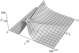
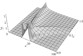
Figure 10: Illustration of the coupling coefficients ${\mathcal{J}_{\ell}\big{[}\mathbf{K},\mathbf{K}^{\prime}\big{]}}$ for ${\ell=10}$ (top) and ${\ell=40}$ (bottom). Here, we chose ${(a,e)=(40,0.15)}$. The vertical axes have been arbitrarily rescaled. As highlighted in the text, a given orbit mostly couples with orbits with similar semi major axes.

In that figure, we note that a given particle is strongly coupled to particles that share similar conserved parameters, in particular similar semi-major axes. Moreover, we note that as $\ell$ increases, the amplitude of the coupling coefficient, $\mathcal{J}_{\ell}$, drastically reduces.

Appendix B The Elsasser coefficients

Let us detail some contraction rules satisfied by the Elsasser coefficients used throughout the paper. Complementary definitions and expressions can be found in Appendix B of Fouvry et al. (2019b). The Elsasser coefficients can be decomposed as

$$E_{\alpha\gamma\delta}=E^{L}_{\ell_{\alpha}\ell_{\gamma}\ell_{\delta}}\,E^{M}_{\alpha\gamma\delta},$$ (38)

where $E^{L}_{\ell_{\alpha}\ell_{\gamma}\ell_{\delta}}$ only depends on ${(\ell_{\alpha},\ell_{\gamma},\ell_{\delta})}$, while $E^{M}_{\alpha\gamma\delta}$ also depends on ${(m_{\alpha},m_{\gamma},m_{\delta})}$. These coefficients satisfy various exclusion rules. In particular, to be non-zero, one has to satisfy

$$\text{(C1)}\mathrel{\mathop{\ordinarycolon}} \,\,|m_{\alpha}|\leq\ell_{\alpha};\;\;|m_{\gamma}|\leq\ell_{\gamma};\;\;|m_{\delta}|\leq\ell_{\delta},$$

$$\text{(C2)}\mathrel{\mathop{\ordinarycolon}} \,\,\ell_{\alpha}+\ell_{\gamma}+\ell_{\delta}\;\text{ is odd},$$

$$\text{(C3)}\mathrel{\mathop{\ordinarycolon}} \,\,|\ell_{\alpha}-\ell_{\gamma}|<\ell_{\delta}<\ell_{\alpha}+\ell_{\gamma}\;\text{ (strict triangular inequality)},$$

$$\text{(C4)}\mathrel{\mathop{\ordinarycolon}} \,\,\text{all pairs }(\ell_{\alpha},m_{\alpha}),(\ell_{\gamma},m_{\gamma}),(\ell_{\delta},m_{\delta})\;\text{ are different}.$$ (39)

In addition, the Elsasser coefficients also follow the symmetry relation ${E_{\alpha\gamma\delta}\!=\!E_{\delta\alpha\gamma}\!=\!-E_{\alpha\delta\gamma}}$. These coefficients also satisfy various contraction rules. As already used in Fouvry et al. (2019b), one has

$$\,\sum_{m_{\gamma},m_{\delta}}E^{M}_{\alpha\gamma\delta}E^{M}_{\beta\gamma\delta}=\delta_{\alpha\beta}\frac{1}{2\ell_{\alpha}+1},$$

$$\,\sum_{\ell_{\delta}}\frac{1}{2\ell_{\alpha}+1}\big{(}E^{L}_{\ell_{\alpha}\ell_{\gamma}\ell_{\delta}}\big{)}^{2}=A_{\ell_{\alpha}}B_{\ell_{\gamma}},$$ (40)

where the first relation only holds when ${(\ell_{\alpha},\ell_{\gamma},\ell_{\delta})}$ satisfy the exclusion rules from Eq. (39). In the previous formula, we also introduced ${A_{\ell}=\ell(\ell+1)}$ as well as ${B_{\ell}=\ell(\ell+1)(2\ell+1)/(8\pi)}$. To these two rules, we finally add the following one

$$\sum_{\ell_{\delta}}\frac{1}{2\ell_{\alpha}+1}A_{\ell_{\delta}}\big{(}E^{L}_{\ell_{\alpha}\ell_{\gamma}\ell_{\delta}}\big{)}^{2}\!=\!A_{\ell_{\alpha}}B_{\ell_{\gamma}}(A_{\ell_{\alpha}}\!+\!A_{\ell_{\gamma}}\!-\!2),$$ (41)

which will prove useful in Appendix D to compute the effect of the separation in orientation in the limit of very close particles.

Appendix C Initial statistics

Let us detail the initial statistics of the test particles’ separation, occurring in the second-expectation from Eq. (18). Throughout the paper, we will consider two different initial statistics, namely a sampling with a fixed angular separation between two test particles, and a smooth sampling following the Von Mises-Fisher statistics.

C.1 Fixed angle separation

A simple route to sample two particles on the unit sphere is to draw them with a constant and given angular separation. To do so, one may draw the orientation of the first particle, $\widehat{\mathbf{L}}_{1}$, uniformly on the sphere. Then, the second orientation, $\widehat{\mathbf{L}}_{2}$, is sampled uniformly on the circle such that ${\widehat{\mathbf{L}}_{1}\!\cdot\!\widehat{\mathbf{L}}_{2}=\cos(\phi_{0})}$, with ${\cos(\phi_{0})\in[-1,1]}$, the fixed angular separation between the two particles. The joint PDF of such a process is given by

$$P(\widehat{\mathbf{L}}_{1},\widehat{\mathbf{L}}_{2})=\frac{1}{8\pi^{2}}\delta_{\mathrm{D}}(\widehat{\mathbf{L}}_{1}\cdot\widehat{\mathbf{L}}_{2}-\cos(\phi_{0})).$$ (42)

As required by Eq. (19), one can compute the statistics of the test particles’ initial separation. It follows from the addition theorem for spherical harmonics, and one gets

$$D_{\ell}=P_{\ell}(\cos(\phi_{0})),$$ (43)

with $P_{\ell}$ the Legendre polynomial.

In the limit of small angular separation, i.e. ${\cos(\phi_{0})\to 1}$, the following Taylor expansion holds

$$P_{\ell}(\cos(\phi_{0}))\simeq 1-\tfrac{1}{2}\ell(\ell+1)(1-\cos(\phi_{0})).$$ (44)

In particular, one recovers that for a vanishing angular separation, ${P_{\ell}(\cos(\phi_{0}))\to 1}$, i.e. ${\mathbf{D}=\mathbf{I}}$. Such a distribution will prove useful to construct the Markovian piecewise prediction presented in Section 4.

C.2 Von Mises-Fisher distribution

The Von Mises-Fisher distribution (Wood, 1994) is characterised by the PDF

$$P(\widehat{\mathbf{L}})=\frac{\kappa}{4\pi\sinh(\kappa)}\,\mathrm{e}^{\kappa\widehat{\mathbf{L}}\cdot\widehat{\mathbf{L}}_{0}}.$$ (45)

In that expression, $\widehat{\mathbf{L}}_{0}$ stands for a preferred direction, and $\kappa$ for the concentration of the PDF. The larger $\kappa$, the smaller is the spread of the PDF on the unit sphere. As such, Eq. (45) is the analog of a Gaussian distribution on the sphere. Sampling the test particles according to that statistics amounts therefore to sampling once $\widehat{\mathbf{L}}_{0}$ uniformly on the sphere, as required by isotropy, and then sampling the test particles according to Eq. (45).

Following Eq. (19), it is then straightforward to compute the statistics of the test particles’ initial separation. One gets

$$D_{\ell}=\frac{\pi\kappa}{2\sinh^{2}(\kappa)}\,\big{(}I_{\ell+1/2}(\kappa)\big{)}^{2},$$ (46)

with $I_{\ell}$ the modified Bessel function of the first kind. In the limit of small angular separations, i.e. ${\kappa\to+\infty}$, one has asymptotically

$$D_{\ell}\simeq 1-\frac{1}{\kappa}\ell(\ell+1).$$ (47)

We recover therefore that for ${\kappa\to+\infty}$, one has ${D_{\ell}\to 1}$, i.e. ${\mathbf{D}=\mathbf{I}}$, so that the initial patch of test particles on the unit sphere is a Dirac delta. Figure 11 illustrates some examples of initial samplings according the PDF from Eq. (45).

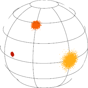
Figure 11: Illustration of the Von Mises-Fisher distribution for three initial patches with ${\kappa=200}$ (yellow), ${1000}$ (orange) and $5000$ (red) resp. The larger $\kappa$ the narrower the distribution of initial orientations. Such a patch is meant to represent a set of co-eval stars which were born with comparable orbital parameters (including orientation). The smaller the initial patch the longer it takes for the VRR-driven dilution to operate.

Appendix D Expectation for separation

Let us detail the calculations leading from Eq. (20) to Eq. (21). We start by performing a second-order Taylor expansion of the matrix exponentials in Eq. (20), so that

$$\mathrm{e}^{\mathbf{\Omega}_{1}}\mathbf{D}\,\mathrm{e}^{-\mathbf{\Omega}_{2}} \,\simeq\big{(}\mathbf{I}+\mathbf{\Omega}_{1}+\tfrac{1}{2}\mathbf{\Omega}_{1}^{2}\big{)}\,\mathbf{D}\,\big{(}\mathbf{I}-\mathbf{\Omega}_{2}+\tfrac{1}{2}\mathbf{\Omega}_{2}^{2}\big{)}$$ (48)

$$\simeq\mathbf{D}\!+\!\mathbf{\Omega}_{1}\mathbf{D}\!-\!\mathbf{D}\mathbf{\Omega}_{2}\!+\!\tfrac{1}{2}\mathbf{\Omega}_{1}^{2}\mathbf{D}+\tfrac{1}{2}\mathbf{D}\mathbf{\Omega}_{2}^{2}-\mathbf{\Omega}_{1}\mathbf{D}\mathbf{\Omega}_{2}.$$

Before computing the ensemble average of that expression, let us first determine the average of $\mathbf{\Omega}_{i}$. Returning to Eq. (17), we have

$$\big{\langle}\mathbf{\Omega}_{i}\big{\rangle}= \,-\!\!\int_{0}^{t}\!\!\mathrm{d}\tau\big{\langle}\mathbf{Q}_{i}(\tau)\big{\rangle}$$

$$\,+\frac{1}{2}\!\!\int_{0}^{t}\!\!\mathrm{d}\tau\!\!\int_{0}^{\tau}\!\!\mathrm{d}\tau^{\prime}\big{\langle}\big{[}\mathbf{Q}_{i}(\tau),\mathbf{Q}_{i}(\tau^{\prime})\big{]}\big{\rangle}.$$ (49)

In that expression, the linear term in $\mathbf{Q}_{i}$ is proportional to the harmonics of the bath. Since the latter is isotropic, these harmonics vanish on average, so that one has ${\langle\mathbf{Q}_{i}\rangle=0}$. Let us now show that the quadratic term also vanishes. Indeed, for indices $i,j$ one has

$$\big{\langle}\big{[}\mathbf{Q}_{i}(\tau)\,\mathbf{Q}_{j}(\tau^{\prime})\big{]}_{\alpha\beta}\big{\rangle}=\sum_{\gamma,\delta,\sigma}E_{\alpha\gamma\sigma}E_{\sigma\delta\beta}$$ (50)

$$\,\times\!\!\int\!\!\mathrm{d}\mathbf{K}\mathrm{d}\mathbf{K}^{\prime}\,\mathcal{J}_{\gamma}\big{[}\mathbf{K}_{i},\mathbf{K}\big{]}\mathcal{J}_{\delta}\big{[}\mathbf{K}_{j},\mathbf{K}^{\prime}\big{]}\big{\langle}f^{\mathrm{b}}_{\gamma}(\mathbf{K},\tau)f^{\mathrm{b}}_{\delta}(\mathbf{K}^{\prime},\tau^{\prime})\big{\rangle}.$$

Using the Gaussian ansatz from Eq. (8) for the bath correlations, as well as the contraction rules for the Elsasser coefficients (see Eq. (40)), we can write

$$\big{\langle}\big{[} \mathbf{Q}_{i}(\tau)\,\mathbf{Q}_{j}(\tau^{\prime})\big{]}_{\alpha\beta}\big{\rangle}=-\delta_{\alpha\beta}A_{\ell_{\alpha}}$$ (51)

$$\times\sum_{\ell}B_{\ell}\!\!\int\!\!\mathrm{d}\mathbf{K}\,\mathcal{J}_{\ell}\big{[}\mathbf{K}_{i},\mathbf{K}\big{]}\mathcal{J}_{\ell}\big{[}\mathbf{K}_{j},\mathbf{K}\big{]}C^{\mathrm{b}}_{\ell}(\mathbf{K},\tau-\tau^{\prime}).$$

Note that this expression is symmetric both w.r.t. ${i\!\leftrightarrow\!j}$ and ${\tau\!\leftrightarrow\!\tau^{\prime}}$, so that the two matrices ${\mathbf{Q}_{i}}$ and $\mathbf{Q}_{j}$ commute on average. As a result, the commutators in Eq. (49) vanish on average, and so does that whole expression, i.e. we have ${\big{\langle}\mathbf{\Omega}_{i}\big{\rangle}=0}$. Hence the terms linear in $\mathbf{\Omega}_{i}$ in Eq. (48) also vanish on average. Following these simplifications, and owing to the fact that $\mathbf{D}$ is a diagonal matrix, we get

$$\big{\langle}\big{[}\mathrm{e}^{\mathbf{\Omega}_{1}}\mathbf{D}\,\mathrm{e}^{-\mathbf{\Omega}_{2}}\big{]}_{\alpha\beta}\big{\rangle} =\delta_{\alpha\beta}D_{\alpha}+\tfrac{1}{2}\delta_{\alpha\beta}D_{\alpha}\big{\langle}\big{[}\mathbf{\Omega}_{1}^{2}+\mathbf{\Omega}_{2}^{2}\big{]}_{\alpha\alpha}\big{\rangle}$$

$$-\sum_{\gamma}D_{\gamma}\big{\langle}\big{[}\mathbf{\Omega}_{1}\big{]}_{\alpha\gamma}\big{[}\mathbf{\Omega}_{2}\big{]}_{\gamma\beta}\big{\rangle},$$ (52)

where in the first line we used Eq. (51) to ensure that only the diagonal coefficients of ${\langle\mathbf{\Omega}^{2}_{i}\rangle}$ are non-zero on average. Given that all these terms are already quadratic in $\mathbf{\Omega}_{i}$, in Eq (17), we may keep only the terms linear in $\mathbf{Q}_{i}$. Subsequently, using Eq. (51) (which remains true for distinct ${i,j}$), we get that the $\mathbf{Q}$ matrices commute on average, and therefore so do the $\mathbf{\Omega}$ matrices. As a consequence, we can then write

$$\big{\langle}\big{[}\mathrm{e}^{\mathbf{\Omega}_{1}}\mathbf{D}\,\mathrm{e}^{-\mathbf{\Omega}_{2}} \big{]}_{\alpha\beta}\big{\rangle}=\delta_{\alpha\beta}D_{\alpha}\!+\!\tfrac{1}{2}\delta_{\alpha\beta}D_{\alpha}\big{\langle}\big{[}\big{(}\mathbf{\Omega}_{1}-\mathbf{\Omega}_{2}\big{)}^{2}\big{]}_{\alpha\alpha}\big{\rangle}$$

$$-\sum_{\gamma}\!\big{(}D_{\gamma}\!-\!\delta_{\alpha\beta}D_{\alpha}\big{)}\big{\langle}\big{[}\mathbf{\Omega}_{1}\big{]}_{\alpha\gamma}\big{[}\mathbf{\Omega}_{2}\big{]}_{\gamma\beta}\big{\rangle}.$$ (53)

Using once again the contraction rules of the Elsasser coefficients (as was done in Eq. (51)), we can rewrite Eq. (53) under the isotropic form

$$\big{\langle}\big{[}\mathrm{e}^{\mathbf{\Omega}_{1}}\mathbf{D}\,\mathrm{e}^{-\mathbf{\Omega}_{2}}\big{]}_{\alpha\beta}\big{\rangle} =\delta_{\alpha\beta}\big{(}D_{\alpha}+\tfrac{1}{2}D_{\alpha}\big{\langle}\big{[}\big{(}\mathbf{\Omega}_{1}-\mathbf{\Omega}_{2}\big{)}^{2}\big{]}_{\alpha\alpha}\big{\rangle}$$

$$-\sum_{\gamma}\big{(}D_{\gamma}\!-\!D_{\alpha}\big{)}\big{\langle}\big{[}\mathbf{\Omega}_{1}\big{]}_{\alpha\gamma}\big{[}\mathbf{\Omega}_{2}\big{]}_{\gamma\alpha}\big{\rangle}\big{)}.$$ (54)

At this stage, since Eq. (54) was obtained through a Taylor expansion, any functional ansatz satisfying this initial expansion is as valid. As it is a polynomial, Eq. (54) is not bounded, and therefore cannot model the correlation’s behaviour for ${t\!\rightarrow\!\infty}$. To circumvent this issue, we now choose the same ansatz as in Fouvry et al. (2019b) and rely on an exponential function. As all the terms are already quadratic in $t$ and the matrix is diagonal, that exponential simply reads

$$\big{\langle}\big{[}\mathrm{e}^{\mathbf{\Omega}_{1}}\mathbf{D}\,\mathrm{e}^{-\mathbf{\Omega}_{2}} \big{]}_{\alpha\beta}\big{\rangle}=\delta_{\alpha\beta}\,D_{\alpha}\exp\!\big{[}\tfrac{1}{2}\big{\langle}\big{[}\big{(}\mathbf{\Omega}_{1}-\mathbf{\Omega}_{2}\big{)}^{2}\big{]}_{\alpha\alpha}\big{\rangle}\big{]}$$

$$\!\!\!\!\times\exp\bigg{[}\sum_{\gamma}\!\frac{D_{\alpha}\!-\!D_{\gamma}}{D_{\alpha}}\big{\langle}\big{[}\mathbf{\Omega}_{1}\big{]}_{\alpha\gamma}\big{[}\mathbf{\Omega}_{2}\big{]}_{\gamma\alpha}\big{\rangle}\bigg{]}.$$ (55)

In Eq. (55), we have recovered Eq. (21) presented in the main text. Finally, one only has to plug in the expression for $\mathbf{\Omega}_{i}$ from Eq. (17), and, following Eq. (51) substitute the bath correlation function by its Gaussian expression from Eq. (8) to get

$$C_{\alpha}^{\mathbf{\Omega}} (t)\,=\exp\bigg{[}-\frac{1}{2}A_{\ell_{\alpha}}\sum_{\ell}B_{\ell}\!\!\int\!\!\mathrm{d}\mathbf{K}\,n(\mathbf{K})$$ (56)

$$\times \,\big{(}\mathcal{J}_{\ell}\big{[}\mathbf{K}_{1},\mathbf{K}\big{]}\!-\!\mathcal{J}_{\ell}\big{[}\mathbf{K}_{2},\mathbf{K}\big{]}\big{)}^{2}\,\frac{2T_{\mathrm{c}}^{2}(\mathbf{K})}{A_{\ell}}\chi\big{[}t\sqrt{A_{\ell}/2}/T_{\mathrm{c}}(\mathbf{K})\big{]}\bigg{]},$$

and

$$\,C_{\alpha}^{\mathbf{D}}(t)=\exp\bigg{[}\sum_{\ell,\ell_{\gamma}}\frac{D_{\ell_{\alpha}}-D_{\ell_{\gamma}}}{(2\ell_{\alpha}+1)D_{\ell_{\alpha}}}\big{(}E_{\ell_{\alpha}\ell\ell_{\gamma}}^{L}\big{)}^{2}$$ (57)

$$\!\times\!\!\int\!\!\!\mathrm{d}\mathbf{K}n(\mathbf{K})\mathcal{J}_{\ell}\!\big{[}\mathbf{K}_{1},\!\mathbf{K}\big{]}\!\mathcal{J}_{\ell}\!\big{[}\mathbf{K}_{2},\!\mathbf{K}\big{]}\frac{2T_{\mathrm{c}}^{2}(\mathbf{K})}{A_{\ell}}\chi[t\sqrt{A_{\ell}/2}/T_{\mathrm{c}}(\mathbf{K})]\bigg{]},$$

with the dimensionless function $\chi$ defined in Eq. (27). In Eq. (57), we also introduced the isotropic component of the Elsasser coefficients ${E_{\ell_{\alpha}\ell\ell_{\gamma}}^{L}}$, whose main properties are briefly recalled in Appendix B.

To conclude this Appendix, let us now give a simplified form of Eq. (55) when the stars share initially very similar orientations. We assume that the initial orientations of the two test particles is drawn with a fixed angular separation, ${\cos(\phi_{0})}$. In Eq. (43), we already characterised such a statistics, and showed that ${D_{\ell}\!=\!P_{\ell}(\cos(\phi_{0}))}$. Let us now assume that this separation is small compared to any other relevant scale of the problem. In practice, this amounts to requiring that ${\ell(\ell+1)\ll{1}/{(1-\cos(\phi_{0}))}}$ for any $\ell$ that significantly contributes to the dynamics.

Relying on the development of $D_{\ell}$ from Eq. (44), we can the use the contraction rule of the Elsasser coefficients from Eq. (41), to rewrite Eq. (21) as

$$C_{\alpha\beta}(t)= \,\delta_{\alpha\beta}\,P_{\ell_{\alpha}}(\cos(\phi_{0}))\,\exp\!\big{[}\!-\tfrac{1}{2}A_{\ell_{\alpha}}\Psi^{-}(\mathbf{K}_{1},\mathbf{K}_{2},t)\big{]}$$

$$\times \,\exp\!\big{[}\!-\tfrac{1-\cos(\phi_{0})}{2}A_{\ell_{\alpha}}\Psi^{+}(\mathbf{K}_{1},\mathbf{K}_{2},t)\big{]},$$ (58)

where $\Psi^{-}$ and $\Psi^{+}$ are given by Eqs. (25) and (26). We refer to the main text for a discussion of the effects associated with each of these terms.

Appendix E Dilution of a population

Let us briefly show how one can naturally expand the expression from Eq. (21) to a population with an arbitrary number of test particles.

Throughout Section 3, we focused on the description of the separation of two particles through their two-point correlation functions (see Eq. (14)) written with spherical harmonics. In that case, all our predictions effectively depend only on ${\cos(\phi)}$, with $\phi$ the angular separation between the two particles. Fortunately, such a result can straightforwardly be used to describe the anisotropies that appear when a larger population of test particles diffuses on the unit sphere, e.g., as illustrated in Fig. 2. Indeed, owing to the large scale potential fluctuations, an initially symmetric patch of test particles can reach very complex, cramped, and anisotropic shapes. In the present appendix, we show how one can easily generalise Eq. (21) to a population of test particles. This is in particular useful to interpret the simulations from Appendix (F).

Let us consider a population of $n$ test particles described its discrete DF

$$f(\widehat{\mathbf{L}},\mathbf{K},t)=\frac{1}{n}\sum_{i=1}^{n}\delta_{\mathrm{D}}(\mathbf{K}-\mathbf{K}_{i})\,\delta_{\mathrm{D}}(\widehat{\mathbf{L}}-\widehat{\mathbf{L}}_{i}(t)),$$ (59)

which satisfies the normalisation convention ${\!\int\!\mathrm{d}\mathbf{K}\mathrm{d}\widehat{\mathbf{L}}\,f=1}$. This DF can naturally be expanded in spherical harmonics as

$$f_{\alpha}(\mathbf{K},t)=\frac{1}{n}\sum_{i=1}^{n}\delta_{\mathrm{D}}(\mathbf{K}-\mathbf{K}_{i})Y_{\alpha}(\widehat{\mathbf{L}}_{i}(t)).$$ (60)

Following Eq. (14), we are interested in the two-point correlation functions of these spherical harmonics. It reads

$$f_{\alpha}(\mathbf{K},t)f_{\beta}(\mathbf{K}^{\prime},t)=\frac{1}{n^{2}}\sum_{i,j=1}^{n} \delta_{\mathrm{D}}(\mathbf{K}-\mathbf{K}_{i})\,\delta_{\mathrm{D}}(\mathbf{K}^{\prime}-\mathbf{K}_{j})$$

$$\times Y_{\alpha}(\widehat{\mathbf{L}}_{i}(t))Y_{\beta}(\widehat{\mathbf{L}}_{j}(t)).$$ (61)

Let us now compute the ensemble average of the previous expression. We assume that the orbital parameters of the test particles are distributed according to some PDF, ${p(\mathbf{K})}$, normalised so that ${\!\int\!\mathrm{d}\mathbf{K}p(\mathbf{K})=1}$, independent of their initial orientations. Paying attention to the cases ${i=j}$ and ${i\neq j}$, we can rewrite Eq. (61) as

$$\big{\langle}f_{\alpha}(\mathbf{K},t)f_{\beta}(\mathbf{K}^{\prime},t)\big{\rangle}= \frac{n(n\!-\!1)}{n^{2}}\,p(\mathbf{K})\,p(\mathbf{K}^{\prime})\,C_{\alpha\beta}(\mathbf{K},\mathbf{K}^{\prime},t)$$

$$+ \frac{1}{4\pi}\frac{1}{n}\,\delta_{\mathrm{D}}(\mathbf{K}-\mathbf{K}^{\prime})\,p(\mathbf{K}),$$ (62)

In that expression, we introduced ${C_{\alpha\beta}(\mathbf{K},\mathbf{K}^{\prime},t)}$ as the two-point correlation of two test particles with orbital parameters $\mathbf{K}$ and $\mathbf{K}^{\prime}$, as already defined in Eq. (14) For ${n\gg 1}$, Eq. (62) naturally becomes

$$\big{\langle}f_{\alpha}(\mathbf{K},t)f_{\beta}(\mathbf{K}^{\prime},t)\big{\rangle}\simeq p(\mathbf{K})\,p(\mathbf{K}^{\prime})\,C_{\alpha\beta}(\mathbf{K},\mathbf{K}^{\prime},t).$$ (63)

Equation (63) shows therefore that the correlation function of a given population of test particles essentially corresponds to the average correlation of particles’ pairs, averaged over realisation of the orbital parameters (that are distributed according to the PDF ${p(\mathbf{K})}$).

To conclude, following Eq. (60), for a population of test particles, a natural observable to consider is therefore

$$\frac{1}{n^{2}}\!\!\sum_{i,j=1}^{n}\!\!\!\big{\langle}Y_{\alpha}(\widehat{\mathbf{L}}_{i}(t)) \,Y_{\beta}(\widehat{\mathbf{L}}_{j}(t))\big{\rangle}$$ (64)

$$\,\simeq\!\!\int\!\!\mathrm{d}\mathbf{K}\mathrm{d}\mathbf{K}^{\prime}\,p(\mathbf{K})\,p(\mathbf{K}^{\prime})\,C_{\alpha\beta}(\mathbf{K},\mathbf{K}^{\prime},t),$$

where we used Eq. (63). In practice, we are mostly interested in the typical angular size of the patch, i.e. the case ${\ell_{\alpha}=\ell_{\beta}=1}$. In that case, Eq. (64) becomes

$$\frac{1}{n^{2}}\!\!\sum_{i,j=1}^{n}\!\!\!\big{\langle}Y_{\alpha}(\widehat{\mathbf{L}}_{i}(t))Y_{\beta}(\widehat{\mathbf{L}}_{j}(t))\big{\rangle} \,=\frac{1}{4\pi}\frac{1}{n^{2}}\sum_{i,j=1}^{n}\langle\cos(\phi_{ij}(t))\rangle$$

$$\,=\frac{1}{4\pi}\bigg{|}\frac{1}{n}\sum_{i=1}^{n}\widehat{\mathbf{L}}_{i}(t)\bigg{|}^{2},$$ (65)

with ${\phi_{ij}(t)}$ the angular separation between the particles ${i,j}$. We finally emphasise that even though each individual orientation is a unit vector, their average, appearing in Eq. (65), is not. More precisely, this average tends to be unitary when the patch of test particles is very localised, and vanishes when the patch becomes isotropic on the unit sphere.

Appendix F Numerical simulations

Let us briefly present the numerical simulations to which our analytical results are compared. The code used to integrate that system is the exact same as that used in Fouvry et al. (2019b), and detailed in Appendix C therein. In a nutshell, at every timestep, the code computes the particles’ instantaneous magnetisations. It has an overall complexity scaling like ${\mathcal{O}(N^{2}\ell_{\mathrm{max}}^{2})}$, with $N$ the total number of particles, and ${\ell_{\mathrm{max}}}$ the maximum harmonic number considered in the pairwise interaction. Once the velocity vectors are computed, particles are displaced forward in time using a fourth-order Runge-Kutta scheme, with a constant global timestep. The present method can benefit from parallelisation when computing the magnetisations, that are seen as contractions of large matrices and vectors.

The simulations used throughout the text are composed as such. The background bath is made of ${N=10^{3}}$ stars. Their conserved quantities ${\mathbf{K}_{i}=(m_{i},a_{i},e_{i})}$ satisfy ${m=m_{\mathrm{min}}}$, ${a_{\mathrm{min}}\leq a\leq a_{\mathrm{max}}}$, and ${e_{\mathrm{min}}\leq e\leq e_{\mathrm{max}}}$. We pick our units so that ${G=m_{\mathrm{min}}=a_{\mathrm{min}}=1}$, and we consider the ranges ${a_{\mathrm{max}}/a_{\mathrm{min}}=100}$, ${e_{\mathrm{min}}=0}$, and ${e_{\mathrm{max}}=0.3}$. Each of these parameters are drawn independently from one another, according to PDFs proportional to ${(\delta_{\mathrm{D}}(m-m_{\mathrm{min}}),a^{1/2},e)}$. Finally, the initial orientations of the background stars are drawn uniformly on the sphere, and interactions are truncated at ${\ell_{\mathrm{max}}=50}$. The background particles are fully self-gravitating, i.e. are all coupled to each other. The timestep of the integration is picked using the exact same method and parameters as in Fouvry et al. (2019b).

On top of that, in order to investigate the separation of neighbour test particles, we also add to the simulation ${n=10^{3}}$ test particles. These are test particles, i.e. they do not contribute to the mean potential, but only probe its instantaneous value. The initial parameters of the test particles, ${\mathbf{K}_{\mathrm{t}}=({m_{\mathrm{t}}},a_{\mathrm{t}},e_{\mathrm{t}})}$, are picked with ${{m_{\mathrm{t}}}=m_{\mathrm{min}}}$, ${9\leq a_{\mathrm{t}}\leq 11}$, and ${e_{\mathrm{min}}\leq e_{\mathrm{t}}\leq e_{\mathrm{max}}}$. Within that range, the parameters are drawn with the same PDFs as for the background particles. For simulations where the test particles have all the same orbital parameters, we used the median value of these distributions, that correspond to ${(a_{\mathrm{t}},e_{\mathrm{t}})\simeq(10,0.21)}$. For each realisations, the initial orientation of the test particles is drawn according to the Von Mises-Fisher distribution from Eq. (45). Adding the test particles to the dynamics does not drastically increase the complexity of the code, as it then scales like ${\mathcal{O}(N(N\!+\!n)\ell_{\mathrm{max}}^{2})}$.

In practice, we performed two sets of simulations of that system: (i) the test particles all have the same orbital parameters, and an initial dispersion in orientation characterised by ${\kappa=5000}$, as defined in Eq. (45); (ii) the test particles have an initial distribution of orbital parameters, and an initial orientation also given by ${\kappa=5000}$. The main interest of the first set of simulations is to allow us to investigate the effect of the separation in orientations, in the absence of any separation stemming from differences in parameters. For each of these simulations, we considered 200 different realisations to perform the ensemble averages.

Appendix G Piecewise prediction

Let us now detail the calculations leading to the piecewise prediction from Section 4, and illustrated in Fig. 6. The goal is to give a simple prediction for the expectation ${\langle\cos(\phi_{i})\rangle}$ corresponding to the timestep ${t_{i}=i\Delta t}$ with ${i\geq 0}$. Thanks to the Markovian assumption, the statistics of ${\cos(\phi_{i+1})}$ is fully determined by the statistics of the previous angle separation ${\cos(\phi_{i})}$ and the properties of the background stochastic noise. As such, we can write

$$\langle\cos(\phi_{i+1})\rangle=\!\!\int\!\!\mathrm{d}(\cos(\phi_{i}))\,\rho_{i}(\cos(\phi_{i}))\,\langle\cos(\phi_{i+1})|\phi_{i}\rangle,$$ (66)

where $\rho_{i}$ is the PDF of ${\cos(\phi_{i})}$, i.e. the statistics of the initial angular separation for the timelapse ${\cos(\phi_{i})\to\cos(\phi_{i+1})}$. In Eq. (66), we also introduced ${\langle\cos(\phi_{i+1})|\cos(\phi_{i})\rangle}$ as the conditional expectation of ${\cos(\phi_{i+1})}$ given the value of ${\cos(\phi_{i})}$, i.e. the expectation of the new angular separation ${\cos(\phi_{i+1})}$ after a time ${\Delta t}$ for test particles initially separated by ${\cos(\phi_{i})}$. As such, in that expectation ${\cos(\phi_{i})}$ is taken to be an initial condition rather than a random variable.

Let us therefore assume that the two test particles are initially separated by ${\cos(\phi_{i})}$. In Appendix C.1, we have already characterised the statistics of such fixed angular separations. Following Eq. (43), we can therefore describe the initial separation of the test particles via the coefficients ${D_{\ell}=P_{\ell}(\cos(\phi_{i}))}$. We can then use the prediction from Eq. (21) to obtain, after a time ${t=\Delta t}$, the conditional expectation for the test particles’ new separation. For any harmonics $\ell$, we write

$$\langle P_{\ell}(\cos(\phi_{i+1}\!))|\cos(\phi_{i})\rangle\!=\!P_{\ell}(\cos(\phi_{i}))\,C_{\ell}^{\mathbf{\Omega}}\!(\Delta t)C_{\ell}^{\mathbf{D}}\!(\Delta t),$$ (67)

with ${C_{\ell}^{\mathbf{\Omega}}(\Delta t)}$ and ${C_{\ell}^{\mathbf{D}}(\Delta t)}$ given by Eq. (21). Since we have ${P_{1}(\cos(\phi_{i+1}))\!=\!\cos(\phi_{i+1})}$, we are mainly interested in the case ${\ell=1}$ of Eq. (67).

Even if the r.h.s. of Eq. (67) is fully known, performing explicitly the integral from Eq. (66) is impossible. Indeed, the PDF of ${\rho_{i}(\cos(\phi_{i}))}$ is unknown, nor can we hope to compute that integral with the intricate integrand from Eq. (67). To proceed further, we rely on a first-order perturbative expansion of the r.h.s. of Eq. (67) for small angular separations, i.e. for ${\cos(\phi_{i})\simeq 1}$. At this stage, the only dependences on ${\cos(\phi_{i})}$ in the r.h.s. of Eq. (67) are through the coefficients ${D_{\ell}=P_{\ell}(\cos(\phi_{i}))}$. In particular, these coefficients only appear in the expression of ${C_{\ell}^{\mathbf{D}}(\Delta t)}$, as given by Eq. (57).

In that limit, Eq. (67) becomes

$$\langle\cos(\phi_{i+1})|\cos(\phi_{i})\rangle =\xi_{0}+\xi_{1}\cos(\phi_{i}),$$ (68)

where the coefficients $\xi_{k}$ are given by

$$\xi_{0} \,=\langle\cos(\phi_{i+1})|\cos(\phi_{i})\rangle\big{|}_{\cos(\phi_{i})=1}-\xi_{1},$$

$$\xi_{1} \,=\frac{\partial}{\partial\cos(\phi_{i})}\bigg{[}\langle\cos(\phi_{i+1})|\cos(\phi_{i})\rangle\bigg{]}_{\cos(\phi_{i})=1}.$$ (69)

Fortunately, in the limit ${\cos(\phi_{i})\to 1}$, we can follow the exact same development as in Eq. (58) to write

$$\langle\cos(\phi_{i+1})|\cos(\phi_{i})\rangle\simeq\cos(\phi_{i})\,\mathrm{e}^{-\Psi^{-}}\mathrm{e}^{-\Psi^{+}(1-\cos(\phi_{i}))}$$ (70)

where we used the fact that ${A_{\ell=1}/2=1}$, and where the functions $\Psi^{-}$ and $\Psi^{+}$ were introduced in Eq. (25) and (26), and are evaluated in ${t=\Delta t}$. Following the definition from Eq. (69), we finally obtain

$$\xi_{0}\,=-\,\mathrm{e}^{-\Psi^{-}}\,\Psi^{+},\;\;\;\xi_{1}\,=\mathrm{e}^{-\Psi^{-}}(1+\Psi^{+}).$$ (71)

At this stage, since the coefficients $\xi_{0}$ and $\xi_{1}$ do not depend anymore on the test particles’ separation, ${\cos(\phi_{i})}$, we can then take the average of the expansion from Eq. (68) w.r.t. ${\cos(\phi_{i})}$, to get the expectation ${\langle\cos(\phi_{i+1})\rangle}$, as defined in Eq. (66). We get

$$\langle\cos(\phi_{i+1})\rangle=\xi_{0}+\xi_{1}\langle\cos(\phi_{i})\rangle,$$ (72)

This inductive definition can be solved explicitly as

$$\langle\cos(\phi_{i})\rangle=q+\xi_{1}^{i}\big{(}\langle\cos(\phi_{0})\rangle-q\big{)},$$ (73)

with ${q=\xi_{0}/(1-\xi_{1})}$, and ${\langle\cos(\phi_{0})\rangle}$ standing for the average angular separation of the test particles at the initial time. In Eq. (73), note that for test particles with identical parameters, one has ${\Psi^{-}=0}$, so that ${q=1}$, while in the generic case, one has ${q\!\geq\!1}$. Finally, even if Eq. (73) depends on the discrete time index, $i$, it can still be viewed as a continuous function of time, provided one makes the replacement ${i\to t/\Delta t}$. Such continuous predictions are plotted in Figs. 6 and 7.

Note that the prediction from Eq. (73) does not rely on the precise shape of the PDFs ${\rho_{i}(\cos(\phi_{i}))}$, as we are ultimately integrating over them. In addition, since the coefficients $\xi_{k}$ only depend on the coupling coefficients, ${\mathcal{J}_{\ell}[\mathbf{K}_{i},\mathbf{K}]}$, they do not need to be recalculated when the initial angular separation, ${\langle\cos(\phi_{0})\rangle}$, is changed, but only when the background bath, i.e. ${n(\mathbf{K})}$, or the parameters of the test particles, i.e. $\mathbf{K}_{1}$ and $\mathbf{K}_{2}$, are changed.

Because it relies on the perturbative expansion from Eq. (68), when ${\cos(\phi_{i})}$ decreases, Eq. (73) becomes inaccurate, and even diverges to ${-\infty}$ at late times. In practice, however, this is not a problem, since Eq. (68) has good behavior up to ${\langle\cos(\phi)\rangle\gtrsim 0.8}$ (see, e.g., Fig. 6). As a result, using this piecewise prediction, we are in a position to properly describe the early separation of neighbours up to ${\phi\lesssim 37^{\circ}}$. This is more than enough for astrophysical applications. Moreover, should one wish to extend this prediction to even larger angular separations, the present piecewise approach can in practice be extended with the analytical prediction from Eq. (21), that rightfully works in regimes where the angular separation between the test particles is large.

Appendix H Restricted $\ell=2$ toy model

The toy model presented in this Appendix serves two main purposes: (i) to illustrate quantitatively the impact of the bath on the test particles in some simplified framework; (ii) to allow for the tuning of the transition PDF on which the Markovian model of Appendix I is based.

Similarly to Roupas et al. (2017); Hamers et al. (2018), we construct our toy model by restricting the VRR interaction to the sole ${\ell=2}$ harmonics, i.e. only the coupling coefficients, ${\mathcal{J}_{\ell}}$, with ${\ell=2}$ are taken to be non-zero. To further simplify the setup, we assume that background cluster is composed only of identical stars. As a result, in Eq. (12), there is a single coupling coefficient, which we denote $\mathcal{J}_{2}$ (which can however vary between different test particles.) Similarly, following Eq. (9), there is a single coherence time for the bath, which we denote $T_{\mathrm{c}}$. In the case ${\ell=2}$, the equations of motion for the test particle can then be rewritten as

$$\frac{\mathrm{d}\widehat{\mathbf{L}}}{\mathrm{d}t}=\widehat{\mathbf{L}}\times\big{(}\mathbf{M}(t)\cdot\widehat{\mathbf{L}}\big{)},$$ (74)

where the time dependent matrix ${\mathbf{M}(t)}$ reads

$$\mathbf{M}(t)=\begin{pmatrix}\eta_{2}&\eta_{-2}&-\eta_{1}\\ \eta_{-2}&-\eta_{2}&-\eta_{-1}\\ -\eta_{1}&-\eta_{-1}&\sqrt{3}\eta_{0}\end{pmatrix},\hfill$$ (75)

where we have set

$$\eta_{m}(t)=\sqrt{B_{2}}\mathcal{J}_{2}f^{\mathrm{b}}_{2m}(t)\,.$$ (76)

Here, the stochastic matrix ${\mathbf{M}(t)}$ contains all the information about the potential fluctuations generated by the background bath.

At any given time, ${\mathbf{M}(t)}$, which is a symmetric matrix, has three orthogonal eigenvectors, that we denote ${\mathbf{e}_{k}}$ (with ${k=1,2,3}$). These vectors define three orientations, and therefore six ‘poles’ on the unit sphere. For any particle standing on one of these poles, one has ${\mathbf{M}(t)\!\cdot\!\widehat{\mathbf{L}}\propto\widehat{\mathbf{L}}}$, so that these are equilibrium points of the dynamics as the cross product from Eq. (74) vanishes. Decomposing any generic ${\widehat{\mathbf{L}}(t)}$ over that same basis, as ${\widehat{\mathbf{L}}(t)=\sum_{k=1}^{3}\Lambda_{k}\mathbf{e}_{k}}$, we can rewrite Eq. (74) under the simpler form

$$\frac{\mathrm{d}\bm{\Lambda}}{\mathrm{d}t}=\pm\,\bm{\Lambda}\times\big{(}\mathbf{D}(t)\cdot\bm{\Lambda}\big{)},$$ (77)

where ${\mathbf{D}(t)}$ is the diagonal matrix, whose entries are the three eigenvalues of ${\mathbf{M}(t)}$, and the global sign depends on the relative order of the eigenvectors. Of course, Eq. (77) remains a quadratic (and stochastic) differential equation hard to generically solve.

To better understand the characteristics of that dynamics, let us assume that ${\widehat{\mathbf{L}}(t)}$ is close to one of the eigenvectors, say ${\mathbf{e}_{a}}$. Assuming ${\Lambda_{a}\gg\Lambda_{b},\Lambda_{c}}$, we can then linearise Eq. (77) to obtain simple linear evolution equations for the two remaining coordinates, ${k=b,c}$, as

$$\frac{\mathrm{d}^{2}\Lambda_{k}}{\mathrm{d}t^{2}}=-\Lambda_{a}^{2}\,(d_{b}-d_{a})(d_{c}-d_{a})\,\Lambda_{k},$$ (78)

with $d_{k}$ the eigenvalues of $\mathbf{D}$. From the structure of Eq. (78), we can note that the stability of the six equilibrium points depends on the eigenvalue with which they are associated (Roupas et al., 2017). Indeed, the equilibrium points associated with the largest and smallest eigenvalues are stable, while the ones associated with the intermediate eigenvalue are unstable.

Following this property, Eq. (78) therefore defines six dynamical regions on the sphere, four of them enforce stable rotating trajectories around the stable points, while the two other unstable regions drive diverging trajectories. We finally note from the non-linearity of Eq. (78) that the frequency for these dynamics depends on the distance to the equilibrium points. This will naturally enforce a phase mixing of particles close to these stable points, as a result of this shear in frequency. In addition to this orientation-induced phase mixing, test particles with different orbital parameters will also shear apart, as their orbital frequencies depend linearly on the coupling coefficients.

On top of this phase mixing, the most efficient way to separate nearby test particles appears in the vicinity of the unstable points which define separatrices on the unit sphere, where test particles get swiftly separated. In Fig. 12, we illustrate the typical orbits of the present toy model.

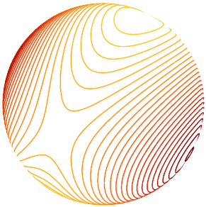
Figure 12: Illustration of trajectories in the toy model from Eq. (74) for a time-independent background noise, i.e. for ${\mathbf{M}(t)\!=\!\mathrm{cst.}}$ One can clearly note the presence of attraction points (e.g., near the pole) and separatrices where the separation of neighbours will be the most efficient.

For such a model, orbits are generically the intersections of the unit sphere with an ellipsoid having the same centre (Roupas et al., 2017). In that figure, one can clearly note the presence of stable regions that source phase mixing, as well as unstable regions associated with separatrices.

At this stage, it is important to emphasise that the previous discussion has been made without taking into account the explicit time-dependence of ${\mathbf{M}(t)}$, i.e. it is only valid for timescales ${t\ll T_{\mathrm{c}}}$. Because of the stochastic changes of ${\mathbf{M}(t)}$, the test particles’ dynamics becomes obviously more intricate on longer timescales. Indeed, as the matrix changes, the eigen-directions, and therefore the six dynamical regions, move around the sphere, so that no point on the sphere remains an equilibrium point. Eventually, the test particles continuously pass from one dynamical region to the other, which keeps distorting their trajectories and stirring them away from one another.

In practice, this reshuffling of the eigen-directions turns out to be the main dynamical process driving the growth of the angular separation between test particles. Indeed, if the eigen-directions were constant, two particles launched with similar directions would likely find themselves within the same dynamical region. Their trajectories would therefore be close to each other, and they would only drift apart through phase mixing. In that case, only if the two particles were initially separated by a separatrix will they have very different trajectories. The closer initially the two particles, the less likely for them sit on two sides of a separatrix. However, once one accounts for the time-dependence of ${\mathbf{M}(t)}$, these separatrices start moving around the sphere. It gets then much more likely that at some point a separatrix will get in between the two test particles. From that moment onwards, the separation between the particles is drastically accelerated, as their trajectories become very different. Hence, it is this succession of rapid stirring induced by the stochastic motion of the separatrices that is the main dynamical driver of the separation of neighbours in the VRR dynamics.

From this discussion, it appears that an essential quantity is therefore the ratio between the ballistic timescale (i.e. the dynamical time for the motion of a test particle in a given and fixed noise) and the coherence timescale (i.e. the time required for a significant modification of the background noise). The ballistic timescale depends primarily on the typical amplitude of the background fluctuations and on the coupling strength between the test particles and the bath. The coherence timescale is given by the correlation time, i.e. by $T_{\mathrm{c}}$ as defined in Eq. (9). If one assumes that the test particles share the same orbital parameters as that of the bath, following Eq. (8), one can show that the ratio of the ballistic and coherence timescales equals $\sqrt{3}$. This implies that both timescales are such that the motion of the test particles and the reshuffling of the eigen-directions happen simultaneously. This further complicates the dynamics, as the lack of timescale separation requires that the two effects are accounted for simultaneously.

Even though this toy model is a useful and insightful tool to understand the dynamics that drive neighbour separation, it is only an approximation of the general VRR dynamics where all harmonics are taken into account. As illustrated in Fig. 13, higher-order harmonics allow for the creation of even more separatrices, which further boost the efficiency of particles’ separation.

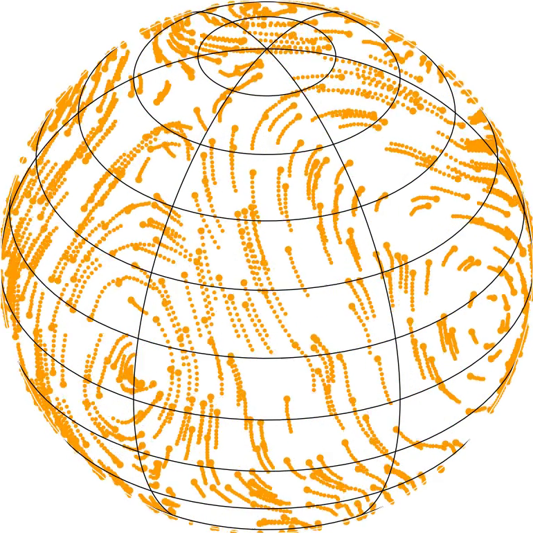
Figure 13: Illustration of the test particles’ trails at late time in numerical simulations, where all the test particles have the same set of orbital parameters (see Appendix F). Stars strikingly seem to rotate for some time around some attraction orientations related to those described in detail in Fig 12 for the toy model. When higher order harmonics contribute to the potential, at any given time, the unit sphere is segmented by many separatrices stemming from the (correlated) potential fluctuations generated by the background stellar cluster. A patch of test particles which happens to pass near one such (transient) separatrix will diffuse apart more swiftly.

In practice, to implement numerically the toy model from Eq. (74), we proceeded as follows. For a given realisation, the stochastic matrix, ${\mathbf{M}(t)}$, is generated by sampling time-correlated processes, ${\eta_{m}(t)}$, that follow the theoretical correlation from Eq. (7). These correlated time series are generated using the method spelled out in Romero & Sancho (1999). Once the background noise has been constructed, the evolution equations for the test particles are integrated using a fourth-order Runge-Kutta method (Press et al., 2007). Finally, in order to avoid late-time biases, following the Rodrigues rotation formula, we used a drift operator adapted to the spherical geometry, which proceeds by rotating the unit vectors rather than by naively translating them.

Appendix I Generating virtual dilutions

In Section 4, we developed a piecewise formalism predicting the average evolution of the angular separation between two neighbours. This approach overcame the main difficulty encountered in Fig. 6, namely it managed to ‘bend’ the prediction downwards to better match the numerical measurements. Unfortunately, by design, the piecewise expression from Eq. (32) can only predict the expectation of the angular separation, namely ${\langle\cos(\phi)\rangle}$. It does not predict any higher-order moments, nor can it generate virtual dilutions, that is random walks of ${\cos(\phi)}$ constructed without integrating the evolution equations (hence, very cheap to produce) and mimicking the statistics of the numerical simulations

At first, it could seem that the approach used in Eq. (31) could be generalised to predict higher-order moments. This would amount to push the perturbative expansion to higher orders, obtaining a recurrent system of equations predicting as many moments of ${\cos(\phi)}$ as wished. Unfortunately, the further the expansion is pushed, the more sensitive it becomes to inaccuracies in the analytical predictions from Eq. (21). In practice, only a first-order expansion, as in Eq. (31), was found to be robust enough.

In this section, our goal is to design a procedure to generate virtual samples of the dilution process. Relying still on the Markovian assumption, we want to construct virtual sequences of angular separations, ${\phi_{0}\!\rightarrow\!\phi_{1}\!\rightarrow\!...\!\rightarrow\!\phi_{n}}$. For simplicity, in all this Appendix we will restrict ourselves to the case where both test particles have identical orbital parameters. As shown in Fig. 5, accounting for additional differences in orbital parameters would yield faster dilutions. As in Eq. (29), we take the transition time ${\Delta t}$ between $\phi_{i}$ and $\phi_{i+1}$ to be ${T_{\mathrm{c}}(\mathbf{K})}$, with $\mathbf{K}$ the parameters of the test particles. The key difference with Section 4 is that now $\phi_{i}$ represents an individual sample of a neighbour separation rather than the average over many realisations. Similarly to Eq. (30), the Markovian assumption implies that the PDF of $\phi_{i+1}$, ${\rho_{i+1}(\phi_{i+1})}$, satisfies

$$\rho_{i+1}(\phi_{i+1})=\!\!\int\!\!\mathrm{d}\phi_{i}\,\rho_{i}(\phi_{i})\,P(\phi_{i+1}|\phi_{i}),$$ (79)

where ${P(\phi_{i+1}|\phi_{i})}$ is the probability that two test particles separated by an angle ${\phi_{i}}$ at time ${t\!=\!i\Delta t}$ evolve to a separation $\phi_{i+1}$ at time ${t\!=\!(i\!+\!1)\Delta t}$. We call this PDF the transition probability. We note that this PDF does not depend on $i$, i.e. the underlying physical process does not explicitly depend on time. This is again a consequence of our Markovian assumption.

Equation (79) is hard to solve analytically, however once the transition PDF, ${P(\phi_{i+1}|\phi_{i})}$, is known, generating samples of random walks consistent with it is easy. In the following, our goal will be to obtain a simple estimate for that PDF, both accurate and straightforward to sample, so that one could easily generate virtual dilutions.

I.1 Finding a suitable ansatz

Because Section 4 only gave us estimates of the average properties of neighbour separation, it cannot provide us with a shape for the transition PDF. We must therefore rely on numerical simulations to characterise it. Unfortunately, given the numerical cost of full VRR simulations (see Appendix F) we cannot use them to obtain enough data to check our estimations of the transition PDF. As such, we use a restricted toy model to perform this exploration. Such a simplified model amounts to assuming that only the harmonics ${\ell=2}$ of the bath drives the VRR dynamics. The main properties of that model are spelled out in Appendix H.

Of course, the ${\ell=2}$ toy model is only an approximation of the full VRR process of neighbour separation, for example, reducing the dilution rate compared to the dynamics driven by the full harmonic range. Yet, because the underlying mechanisms remain the same, we expect the functional form of the transition PDF to be similar between the two cases.

In Fig. 14, we show a numerical measurement in the toy model of the transition PDF, ${P(\phi|\phi_{0})}$.

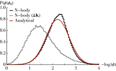
Figure 14: Illustration of the conditional PDF, ${P(\phi|\phi_{0})}$, for the angle $\phi$, in radians, separating two test particles after a time ${\Delta t}$ (see Eq. (29)) as measured in the ${\ell=2}$ toy model. Here, the two test particles have the same orbital parameters, were initially separated by ${\phi_{0}=5^{\circ}}$, and the histogram was obtained over ${500\,000}$ realisations of the toy model. The analytical prediction is given by the log-normal ansatz from Eq. (80), with parameters estimated using Eq. (21). In that plot, we also added the same measurement for simulations where the two test particles differ by a factor ${1.3}$ in their coupling factor to the bath, which naturally accelerates the growth of their angular separation.

Rather than considering ${\cos(\phi)}$ as the variable of interest, we used ${-\log(\phi)}$, whose scale invariance better handles the regime of very small angular separations. In the absence of any separation in orbital parameters, we note that the transition PDF for ${-\log(\phi)}$ is consistent with a normal distribution. In that case, we hint therefore from the numerical simulations that the transition PDF, ${P(\phi_{i+1}|\phi_{i})}$, can be approximated with a log-normal distribution. As such, we assume

$$P(\phi|\phi_{0})=\frac{1}{\phi\,\sigma\sqrt{2\pi}}\exp\bigg{[}-\frac{(-\log(\phi)-\mu)^{2}}{2\sigma^{2}}\bigg{]}.$$ (80)

This a key assumption to be able to generate virtual particles’ separations.

Even though Fig. 14 only corresponds to one particular set of orbital parameters and initial angles, we investigated these transition probabilities for a wide range of orbital parameters and initial angles, and always recovered normal-like distributions. Of course, the ansatz from Eq. (80) ultimately breaks down when the initial angle, ${\phi_{0}}$, becomes too large, since the domain of the normal distribution is not bounded and overflows the range ${-\log(\pi)\leq-\log(\phi)\leq+\infty}$. In practice, we found that this ansatz works well for angles ${\phi\lesssim 45^{\circ}}$.

I.2 Estimating the parameters of the transition distribution

Having identified a plausible ansatz for the transition PDF, we must now use the analytical prediction from Eq. (21) to estimate the two parameters of Eq. (80), namely $\mu$ and $\sigma$.

The moments of the distribution from Eq. (80) generically read

$$\langle\phi^{n}|\phi_{0}\rangle=\exp\!\big{[}\!-n\mu+\tfrac{1}{2}n^{2}\sigma^{2}\big{]}.$$ (81)

From the estimation of ${\langle\phi^{2}|\phi_{0}\rangle}$ and ${\langle\phi^{4}|\phi_{0}\rangle}$ one can then estimate the parameters of the log-normal distribution from Eq. (80). Indeed, one has

$$\mu=\tfrac{1}{4}\log\!\bigg{[}\frac{\langle\phi^{4}|\phi_{0}\rangle}{\langle\phi^{2}|\phi_{0}\rangle^{4}}\bigg{]};\;\;\;\sigma^{2}=\tfrac{1}{4}\log\!\bigg{[}\frac{\langle\phi^{4}|\phi_{0}\rangle}{\langle\phi^{2}|\phi_{0}\rangle^{2}}\bigg{]}.$$ (82)

To estimate these moments, we rely once again on a perturbative development of Eq. (21). For identical particles, we have $C^{\mathbf{\Omega}}_{\ell}=1$. Therefore, taking ${\ell_{\alpha}=1}$ in Eq. (57), we obtain

$$\langle\cos(\phi) |\phi_{0}\rangle\!=\!\cos(\phi_{0})\exp\!\bigg{[}\!\sum_{\ell}\!\frac{\cos(\phi_{0})\!-\!P_{\ell}(\cos(\phi_{0}))}{3\cos(\phi_{0})}\!\big{(}E^{L}_{1\ell\ell}\big{)}^{2}$$

$$\,\times\!\!\int\!\!\mathrm{d}\mathbf{K}\,n(\mathbf{K})\mathcal{J}_{\ell}^{2}\big{[}\mathbf{K}_{1},\mathbf{K}\big{]}T_{\mathrm{c}}^{2}(\mathbf{K})\chi[\Delta t/T_{\mathrm{c}}(\mathbf{K})]\bigg{]}.$$ (83)

Placing ourselves in the limit of small angular separations, we can expand both sides of Eq. (83) to obtain

$$1-\tfrac{1}{2}\langle\phi^{2}|\phi_{0}\rangle+\tfrac{1}{24}\langle\phi^{4}|\phi_{0}\rangle\simeq 1-\tfrac{1}{2}\beta_{2}\,\phi_{0}^{2}+\tfrac{1}{24}\beta_{4}\,\phi_{0}^{4},$$ (84)

where the coefficients

$$\beta_{2}=-\frac{\partial^{2}\langle\cos(\phi)|\phi_{0})\rangle}{\partial\phi_{0}^{2}};\;\;\;\beta_{4}=\frac{\partial^{4}\langle\cos(\phi)|\phi_{0}\rangle}{\partial\phi_{0}^{4}}$$ (85)

are somewhat too intricate to be written down explicitly here but can easily be computed numerically. The next stage of the calculation is to identify terms order by order in Eq. (85). As such, we write

$$\langle\phi^{2}|\phi_{0}\rangle=\beta_{2}\,\phi_{0}^{2};\;\;\;\langle\phi^{4}|\phi_{0}\rangle=\beta_{4}\,\phi_{0}^{4}.$$ (86)

Of course, this identification is only approximate as the average term ${\langle\phi^{2}|\phi_{0}\rangle}$ also contains residual contributions in ${\phi_{0}^{4}}$, in an unknown proportion. Figure 15 compares numerical measurements of ${\langle\phi^{2}|\phi_{0}\rangle}$ and ${\langle\phi^{4}|\phi_{0}\rangle}$ with the predictions from Eq. (86), for a wide range of values of $\phi_{0}$.

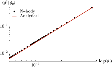
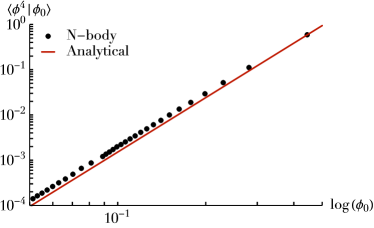
Figure 15: Illustration of the moments ${\langle\phi^{2}|\phi_{0}\rangle}$ and ${\langle\phi^{4}|\phi_{0}\rangle}$, of the transition PDF, ${P(\phi|\phi_{0})}$ (see Eq. (79)), as a function of the initial separation angle $\phi_{0}$ for test particles with the same parameters evolving within the ${\ell=2}$ toy model. All the angles are expressed in radians. Here, the $N$-body measurements were obtained from histograms similar to the one of Fig. 14, while the analytical prediction was obtained following Eq. (86). We observe a good agreement in a wide range of initial angular separations.

While the agreement in Fig. 15 is good, it was only performed for the ${\ell=2}$ toy model. It therefore remains somewhat unclear whether or not such relations would still always be satisfied in the full VRR model.

I.3 Sampling virtual dilutions

In Eq. (80), we identified a simple ansatz for the transition PDF, ${P(\phi|\phi_{0})}$. And following Eqs. (82) and (86), we can use the analytical prediction from Eq. (83) to explicitly estimate the two parameters of that PDF. We note that the coefficients $\beta_{2}$ and $\beta_{4}$ from Eq. (86) solely depend on the conserved orbital parameters of the test stars, i.e. for a given pair of particles, they only have to be computed once.

In Fig. 16, we illustrate examples virtual random walks generated using that estimated transition PDF.

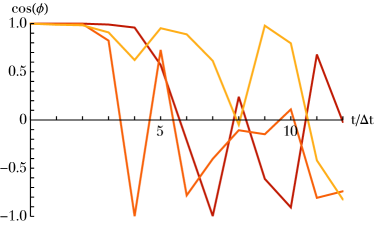
Figure 16: Illustration of three virtual random walks in orientation generated using the ansatz from Eq. (80), and set to match the numerical simulation presented in Fig. 4. Here, we find that test particles separate on comparable timescales, but, as expected from the Markovian assumption, the virtual dilutions cannot mimic any of the short time variations observed in the simulations.

These virtual random walks should be compared to the ones from Fig. 4 directly observed in numerical simulations. Of course, given that the Markovian approach only predicts the angular separation every ${\Delta t}$, the virtual separations from Fig. 16 cannot capture the short time variations present in the numerical simulations. As the motion of the test particles is essentially ballistic on timescales ${\lesssim\Delta t}$, the most important features of the random walks are none the less correctly captured. Indeed, we recover that the timescale for the full separation of the test particles, a few ${\Delta t}$, is similar between the two figures. We also find that both figures exhibit large angular oscillations on timescales ${\gtrsim\Delta t}$.

Once one can create virtual separations of test particles, it only remains to average over them to obtain a Markovian prediction for the expectation of the neighbour separation, i.e. the quantity ${\langle\cos(\phi)\rangle}$. This is illustrated in Fig. 5, where we recover a good agreement between the numerical simulations (for the full VRR model) and the present approach based on virtual realisations of the stochastic dynamics of pair separation.

Appendix J A stellar cusp around SgrA*

Let us detail here the calculations presented in Section 5 to compute the rate of neighbour separation in an infinite power-law stellar distribution around a supermassive BH.

In order to mimic SgrA*, we take the mass of the central BH to be ${M_{\bullet}=4.3\!\times\!10^{6}M_{\odot}}$ (Gillessen et al., 2017). The stellar population is assumed to be single mass, with ${m_{\star}=1\,M_{\odot}}$, so that the mass of the background star is given by the PDF ${f_{m}(m)=\delta_{\mathrm{D}}(m-m_{\star})}$. The stellar distribution of eccentricities is supposed to be thermal (Merritt, 2013), i.e. ${f_{e}(e)=2e}$. We also assume that the number of stars per unit $a$ follows a power-law distribution of the form

$$n_{a}(a)=\frac{N_{0}}{a_{0}}\,\bigg{(}\frac{a}{a_{0}}\bigg{)}^{2-\gamma},$$ (87)

with $a_{0}$ a given scale semi-major axis. In that expression, we also introduced ${N_{0}=g(\gamma)N(\!<\!a_{0})}$ with the normalisation function

$$g(\gamma)=2^{-\gamma}\,(3-\gamma)\,\sqrt{\pi}\,\frac{\Gamma[1\!+\!\gamma]}{\Gamma[\gamma-\tfrac{1}{2}]}.$$ (88)

Here, ${N(\!<\!a_{0})}$ stands for the number of stars physically within a sphere of radius $a_{0}$ from the centre. In practice, for the numerical applications, we used ${a_{0}\!=\!r_{\mathrm{h}}\!=\!2\,\mathrm{pc}}$ the sphere of influence of SgrA*, and as such used ${N(\!<\!a_{0})=4.3\!\times\!10^{6}}$. Following the normalisation of ${n(\mathbf{K})}$ from Eq. (8), we write the background bath’s DF as ${n(m,a,e)\!=\!f_{m}(m)\,f_{e}(e)\,n_{a}(a)/(4\pi)}$.

When adding IMBHs to the background distribution, we assume that they are all of the same individual mass ${m_{\bullet}=100M_{\odot}}$. For simplicity, we also assume that they follow a power law distribution in semi-major axes, as well as a thermal distribution of eccentricities. Finally, we systematically normalise the PDFs so that the total enclosed stellar mass within SgrA*’s sphere of influence remains the same, i.e. we have

$$M_{\star}(\!<\!a_{0})+M_{\mathrm{IMBH}}(\!<\!a_{0})=M_{\bullet},$$ (89)

with ${M_{\star}(\!<\!a_{0})=m_{\star}N(\!<\!a_{0})}$, and similarly for the IMBHs. Equation (89) is used in Fig. 9 to define the mass fraction of IMBHs.

References

- Abbott et al. (2016) Abbott B. P., et al., 2016, Phys. Rev. Lett., 116, 061102
- Alexander (2017) Alexander T., 2017, ARA&A, 55, 17
- Bahcall & Wolf (1976) Bahcall J. N., Wolf R. A., 1976, ApJ, 209, 214
- Bahcall & Wolf (1977) Bahcall J. N., Wolf R. A., 1977, ApJ, 216, 883
- Bar-Or & Alexander (2016) Bar-Or B., Alexander T., 2016, ApJ, 820, 129
- Bar-Or & Fouvry (2018) Bar-Or B., Fouvry J.-B., 2018, ApJ, 860, L23
- Bartko et al. (2009) Bartko H., et al., 2009, ApJ, 697, 1741
- Berti et al. (2006) Berti E., Cardoso V., Will C. M., 2006, Phys. Rev. D, 73, 064030
- Blanes et al. (2009) Blanes S., Casas F., Oteo J. A., Ros J., 2009, Phys. Rep., 470, 151
- Cohn & Kulsrud (1978) Cohn H., Kulsrud R. M., 1978, ApJ, 226, 1087
- Do et al. (2019) Do T., et al., 2019, BAAS, 51, 530
- Eilon et al. (2009) Eilon E., Kupi G., Alexander T., 2009, ApJ, 698, 641
- Event Horizon Telescope Collab. et al. (2019) Event Horizon Telescope Collab. et al., 2019, ApJ, 875, L1
- Fouvry et al. (2019a) Fouvry J.-B., Bar-Or B., Chavanis P.-H., 2019a, Phys. Rev. E, 99, 032101
- Fouvry et al. (2019b) Fouvry J.-B., Bar-Or B., Chavanis P.-H., 2019b, ApJ, 883, 161
- Genzel et al. (2010) Genzel R., Eisenhauer F., Gillessen S., 2010, Rev. Mod. Physics, 82, 3121
- Gillessen et al. (2017) Gillessen S., et al., 2017, ApJ, 837, 30
- Gravity Collab. et al. (2020) Gravity Collab. et al., 2020, A&A, 636, L5
- Habibi et al. (2017) Habibi M., et al., 2017, ApJ, 847, 120
- Hamers et al. (2018) Hamers A. S., Bar-Or B., Petrovich C., Antonini F., 2018, ApJ, 865, 2
- Hopman & Alexander (2006) Hopman C., Alexander T., 2006, ApJ, 645, 1152
- Kocsis & Tremaine (2011) Kocsis B., Tremaine S., 2011, MNRAS, 412, 187
- Kocsis & Tremaine (2015) Kocsis B., Tremaine S., 2015, MNRAS, 448, 3265
- Kormendy & Ho (2013) Kormendy J., Ho L. C., 2013, ARA&A, 51, 511
- Meiron & Kocsis (2018) Meiron Y., Kocsis B., 2018, ApJ, 855, 87
- Merritt (2013) Merritt D., 2013, Dynamics and Evolution of Galactic Nuclei. Princeton Univ. Press
- Portegies Zwart & McMillan (2002) Portegies Zwart S. F., McMillan S. L. W., 2002, ApJ, 576, 899
- Press et al. (2007) Press W., et al., 2007, Numerical Recipes 3rd Ed.. Cambridge Univ. Press
- Rauch & Tremaine (1996) Rauch K. P., Tremaine S., 1996, New Astron., 1, 149
- Romero & Sancho (1999) Romero A. H., Sancho J. M., 1999, J. Comput. Phys., 156, 1
- Roupas et al. (2017) Roupas Z., Kocsis B., Tremaine S., 2017, ApJ, 842, 90
- Shapiro & Marchant (1978) Shapiro S. L., Marchant A. B., 1978, ApJ, 225, 603
- Szölgyén & Kocsis (2018) Szölgyén Á., Kocsis B., 2018, Phys. Rev. Lett., 121, 101101
- Takács & Kocsis (2018) Takács Á., Kocsis B., 2018, ApJ, 856, 113
- Tremaine (2020) Tremaine S., 2020, MNRAS, 493, 2632
- Vasiliev (2017) Vasiliev E., 2017, ApJ, 848, 10
- Wood (1994) Wood A. T., 1994, Commun. Stat.-Simul. Comput., 23, 157
- Yelda et al. (2014) Yelda S., et al., 2014, ApJ, 783, 131