On the dynamical interaction between overshooting convection and an underlying dipole magnetic field - I. The non-dynamo regime
Abstract
Motivated by the dynamics in the deep interiors of many stars, we study the interaction between overshooting convection and the large-scale poloidal fields residing in radiative zones. We have run a suite of 3D Boussinesq numerical calculations in a spherical shell that consists of a convection zone with an underlying stable region that initially compactly contains a dipole field. By varying the strength of the convective driving, we find that, in the less turbulent regime, convection acts as turbulent diffusion that removes the field faster than solely molecular diffusion would do. However, in the more turbulent regime, turbulent pumping becomes more efficient and partially counteracts turbulent diffusion, leading to a local accumulation of the field below the overshoot region. These simulations suggest that dipole fields might be confined in underlying stable regions by highly turbulent convective motions at stellar parameters. The confinement is of large-scale field in an average sense and we show that it is reasonably modeled by mean-field ideas. Our findings are particularly interesting for certain models of the Sun, which require a large-scale, poloidal magnetic field to be confined in the solar radiative zone in order to explain simultaneously the uniform rotation of the latter and the thinness of the solar tachocline.
keywords:
(magnetohydrodynamics) MHD – convection – stars: interiors – Sun: interior–Sun: magnetic fields1 Introduction
The interface between the outer convection zone and inner radiative zone of solar-type stars is a region of crucial importance for stellar evolution in terms of its dynamical role in the transport of chemical species and angular momentum, and for the generation of magnetic fields. In this series of papers, we investigate this region in detail using numerical simulations. Our previous paper (Korre, Garaud & Brummell, 2019) concentrated on purely hydrodynamic processes connecting these two zones, and here we turn to the study of magnetohydrodynamic processes.
Magnetism is arguably the most readily dismissed aspect of stellar astrophysics, despite the fact that magnetic fields are undeniably ubiquitous at all stellar masses and all stages of stellar evolution (see Mestel, 1999). Magnetic fields are expected to be found everywhere in a given star, from the core to the surface, and in both radiative and convective regions. In the highly turbulent convection zones of solar-type stars, even the weakest seed field can be amplified through dynamo action, up to amplitudes that are dynamically significant and often observable using various techniques including starspot tracking and Zeeman imaging, for instance (see the review by Donati & Landstreet, 2009). In the far more quiescent underlying radiation zones, by contrast, any resident magnetic field is usually thought to be of primordial origin or to originate from a nearby convective region through advection or diffusion (Garaud, 1999; Tobias et al., 2001, see; Spruit, 1999, although for alternative theories see also). Regardless of their origin, radiation zone fields are usually thought to be large-scale, because small-scale fields would decay on a time-scale that is short compared with the stellar evolution time-scale.
The main impact of large-scale magnetic fields in stellar radiative zones comes from their ability to transport angular momentum very efficiently through magnetic stresses. In ideal MHD (i.e. in a plasma where the magnetic diffusivity is zero), Ferraro’s law of isorotation (Ferraro, 1937) states that the rotation rate of a fluid is forced to be constant along magnetic field lines. Although stellar plasmas have finite diffusivity, the latter is very small in stellar radiation zones, and Ferraro’s isorotation law applies even if the field amplitude is very small. As demonstrated by Mestel & Weiss (1987), a field as low as a few mG is in principle capable of imposing a roughly uniform rotation in the star’s radiative zone. Ferraro’s isorotation law has important observable consequences for the evolution of the angular velocity profile within solar-type stars undergoing magnetic spin-down. Charbonneau & MacGregor (1993) studied this problem and demonstrated that the overall response of the star’s rotation profile to the spin-down depends crucially on whether an assumed large-scale poloidal field is entirely confined to the radiative interior (i.e. such that in the convective zone), or whether these field lines extend into the overlying convection zone (i.e. such that in the convective zone). In the former case, each zone ultimately ends up rotating almost uniformly, but with different rotation rates. In the latter case, the radiative and convective zones are magnetically connected and the entire star rotates almost uniformly. The rotation profile within the star thus strongly depends on the field’s geometry (confined vs. unconfined).
There is a wealth of observational evidence for both types of configurations in stars of all ages. Observations of the rotation rates of solar-type stars in aMyr-old stellar cluster (Irwin et al., 2007) show that a two-zone model is required for slowly-rotating stars in the mass range , suggesting they might have a confined field structure. Rapid rotators in the same mass range are consistent with uniform rotation, by contrast, suggesting an open field structure. The Sun has been observed (through helioseismology) to possess an almost uniformly rotating inner radiative zone, whereas the outer convection zone rotates differentially with a faster equator and slower poles (Gough et al., 1996). The two zones are separated by a thin shear layer called the solar tachocline. Gough & McIntyre (1998) argued that this could only be explained by the presence of an embedded primordial magnetic field, strictly confined below the base of the convection zone. In red giant branch (RGB) stars, finally, the ratio of the core to envelope rotation rates observed using asteroseismology is far lower than what one would expect from angular momentum conservation only (Beck et al., 2012; Mosser et al., 2012; Marques et al., 2013; Aerts, Mathis & Rogers, 2019, for a review, see also). Angular momentum transport by a combination of large-scale magnetic fields and large-scale flows could provide an explanation for the increased dynamical coupling between the core and the envelope, but would require a confined field structure, as in the Gough & McIntyre (1998) model (see, e.g. Oglethorpe & Garaud, 2013).
In all examples described above, however, the question of how and when a poloidal magnetic field might be confined is still essentially unanswered. For example, Charbonneau & MacGregor (1993), Rüdiger & Kitchatinov (1997) and MacGregor & Charbonneau (1999) assumed a given confined poloidal field shape, and only investigated the dynamical interaction between this field and the angular velocity profile of the star. Gough & McIntyre (1998) were the first to model the confinement of the magnetic field self-consistently, but their model was two-dimensional, and took the form of a steady-state boundary layer analysis. Magnetic confinement in their paper was defined as the ability of the meridional flows to advect the poloidal field downward in a way that compensates the diffusion of the field outward. As a result, the amplitude of the poloidal field was found to decrease exponentially away from this “advection-diffusion" layer. This idea was essentially confirmed by Acevedo-Arreguin, Garaud & Wood (2013), who found steady-state nonlinear numerical solutions of the Gough & McIntyre (1998) model exhibiting confinement (see also Wood & McIntyre, 2011; Wood, McCaslin & Garaud, 2011).
Until the early 2000s, theoretical ideas associated with magnetic confinement primarily revolved around slow, laminar flows, and the question of the role of fast turbulent processes naturally arose (especially as the ability to model 3D time-dependent MHD through super-computing became more prevalent). To understand why, it is useful to split the field and the flow into large scales ( and ) and fluctuations ( and ), such that and and consider again the evolution of large-scale magnetic fields and flows. Beyond its interaction with the mean flow , the evolution of the mean field now also depends on the fluctuation-induced electromotive force (e.m.f.) (where denotes a spatio-temporal or ergodic averaging process), while that of depends on the Reynolds and Lorentz stresses and , respectively. Deep in the radiative zones, where small-scale fluctuations are very weak, these terms are likely not very large. However, in the vicinity of the interface between a radiative zone and a convective zone, which is precisely the region of interest, these terms are expected to be much larger due to the ambient turbulence associated with convective overshooting motions.
That being the case poses several problems. First, it is unlikely that Ferraro’s isorotation theorem, which was derived under very restrictive conditions, continues to apply “as is" for the large-scale field and flow in that region. As such, the magnetic field confinement, which many argued would be required to explain some of the observations, might no longer be necessary. Second, since the convection zone itself is likely the seat of a dynamo (which is one of the manifestations of the electromotive force) and therefore a source of magnetic field, confinement in the sense defined by Charbonneau & MacGregor (1993) or Gough & McIntyre (1998) is not possible in the first place. Instead, the magnetohydrodynamical coupling between the convective envelope and the radiative zone will likely be due to a combination of many different processes, including the previously discussed interaction of the large-scale flows and large-scale fields, but now also involving the interaction of the small-scale flows and small-scale fields, some of which are produced by dynamo action in the convection zone, and some of which are produced locally by the interaction of the overshooting motions with the large-scale radiative zone field. To study this complex problem, it is essential to break free of the traditional, two-dimensional, quasi-steady view of stellar magnetic fields, and to solve the full 3D, time-dependent MHD equations, including rotation, in a spherical coordinate system. The numerical complexity of this task is so formidable, that it is effectively presently unachievable. As such, we are forced to use simplified models, that may be limited spatially to a small region of the star, and/or ignore some of the aforementioned processes, and/or use governing parameters that are far from those of real stars.
One of the most complete studies using this simplified approach was presented by Tobias et al. (2001) (see also Tobias et al., 1998). Considering only a small region of the star located around the base of the convection zone, they performed 3D, nonlinear compressible simulations of penetrative convection at the interface between a convection zone and a radiative zone, and investigated its effect on the transport of magnetic fields. For the wide range of parameters they examined, they found that any initial configuration of a large-scale horizontal magnetic field placed in the Cartesian box would be redistributed (or “pumped") so that the majority of it resides in the radiative zone just below the overshoot zone, where it might eventually diffuse. Note that Tobias et al. (2001) studied the effects of rotation on this turbulent confinement or pumping but did not attempt to include or study the effects of any large-scale meridional motions, which are central to the slow laminar confinement of Gough & McIntyre (1998). More recently, Wood & Brummell (2018) built on the work of Tobias et al. (2001) whereby they included a forced “differential rotation" in the convection zone, which allowed them to drive and study the impact of large-scale meridional flows in the presence of turbulence. They found that, with careful parameter selection, the mean magnetic field in the radiation zone can be confined by the meridional flows, and therefore impose uniform rotation to that region. The turbulence in their simulations was however fairly mild and the overshooting motions on their own were not be able to confine the field in the absence of meridional flows, contrary to prior claims made by Garaud & Rogers (2007) using 2D numerical simulations, and by Kitchatinov & Rüdiger (2008) using parametric models for magnetic pumping. Finally, Strugarek, Brun & Zahn (2011) (see also Brun & Zahn, 2006) performed fully 3D anelastic simulations in a whole-Sun spherical geometry, which had the scope to allow for both slow laminar and fast turbulent confinement effects. The choice of global geometry forced them to use model parameters that are too viscously dominated, however, and neither slow laminar nor fast turbulent confinement were found (see the discussion of Acevedo-Arreguin et al., 2013).
While all the case studies described above provide important insight into the problem, they are still largely preliminary, and cannot easily be used to make predictions on the magnetic coupling between the radiation zone and convection zones of stars other than the Sun. To do so would require a more fundamental understanding of the various processes involved, how they depend on stellar parameters, and how they interact with one another to affect the overall rotation profile of the star. By isolating some of these processes and studying them numerically in a systematic way, it is possible to gain a better understanding of their dependence on the model parameters (which is crucial to the extrapolation from numerical simulations to stellar conditions). This is the approach we are taking in this series of papers. We use 3D spherical Direct Numerical Simulations (DNS), and starting with the simplest problems, gradually add complexity. Our initial work in Korre et al. (2019) omits rotation and examined the question of overshooting convection only. In this work, we expand on Korre et al. (2019) to study the interaction of the overshooting convection with an initially embedded magnetic field. We ignore the effects of rotation in order to examine turbulent confinement in the absence of organized meridional flows (which, as discussed earlier, are an inevitable consequence of rotation). By doing so, we also ignore the effects of rotation on the convective eddies, which is perhaps not a good approximation near the base of the solar convection zone where the rotation rate is comparable to the Brunt-Väisälä frequency . As such, our findings in this paper will not be directly applicable to the present-day Sun, but would be more relevant to more slowly rotating stars for which . We also start by selecting convective parameters for which there is no dynamo, deferring the dynamo case to the next paper in the series. Finally we select an initial field whose amplitude is small enough not to affect the overshooting motions or the convection. As a result, the dominant interaction in this model is that of the overshooting turbulence on the initially large-scale, embedded field.
This problem, even though very simple a priori, already reveals substantial complexity. We attempt to examine our results under the frameworks for magnetic transport that have been readily used before. The most common of these is mean-field theory, where the electromotive force is modeled as , where is the symmetric part of a tensor associated with the generation of large-scale poloidal magnetic fields from toroidal fields, is the anti-symmetric part of the same tensor related to magnetic pumping and is associated with turbulent diffusion. The -effect (see Krause & Raedler, 1980; Cattaneo & Vainshtein, 1991) is associated with the turbulent intensification of magnetic gradients and leads to a faster removal of the field. Some other well-known phenomenologies can be related to these ideas, such as the concept of “magnetic flux expulsion" (Weiss, 1966), where magnetic flux is expelled from regions of circular streamlines and becomes concentrated at the edges of the convective eddies. The - effect is the mean-field manifestation of “diamagnetic pumping", which more generally refers to the transport of a magnetic field down a gradient of turbulent intensity, i.e. in the direction of decreasing turbulence. This process is particularly important in solar-type stars, where the turbulent diffusivity is much larger in the convection zone than in the radiative zone (see, e.g. Kitchatinov & Rüdiger, 2008).
The paper is organized as follows: In Section 2, we describe the model setup along with the initial conditions and the boundary conditions. In Section 3, we present our numerical results for four different Rayleigh numbers (where the Rayleigh number is the ratio of the buoyancy force over the viscosity and the thermal diffusivity and measures the strength of the convective driving) and compare the DNS results with the exact solution of the induction equation in the absence of fluid motion, i.e. the purely diffusive case. In Section 4, we introduce a mean-field model approach to further explain and categorize the observed dynamics. Finally, in Section 5, we summarize and discuss our results, while in Section 6, we conclude with their implications in the astrophysical context.
2 Model set-up
We are interested in studying the dynamics associated with the turbulent transport of magnetic fields between different regions on fast time-scales. As discussed above, we omit rotation in order to isolate the turbulent confinement process from the laminar confinement associated with the slow rotationally-driven large-scale meridional flows. We solve the MHD version of the Spiegel-Veronis-Boussinesq equations (Spiegel & Veronis, 1960) in a non-rotating spherical shell, knowing that even though the Boussinesq approximation might not be the most appropriate choice for astrophysical flows, it is still relevant when modeling deeper stellar interior regions, where the density stratification is small. This allows us to explore a parameter regime with larger Rayleigh numbers and a lower Prandtl number and magnetic Prandtl number than those typically used in spherical compressible or anelastic simulations.
Our setup is similar to the one used in Korre et al. (2019), with a two-layered system that consists of a convectively unstable zone (CZ) lying on top of a stably stratified radiative zone (RZ). The spherical shell has an outer radius , and inner radius , while the CZ-RZ interface is located at . Within the radiative zone, we assume the presence of an initially compactly-contained pre-existing dipole magnetic field (i.e. for ) and wish to study the evolution of this field. We solve the three-dimensional (3D) magnetohydrodynamic (MHD) Navier-Stokes equations under the Boussinesq approximation, and assume that there is a non-zero adiabatic background temperature gradient to account for weak compressibility (Spiegel & Veronis, 1960). We use constant thermal expansion coefficient (where here is different from the one associated with the effect described in Section 1 and in Section 4), viscosity , thermal diffusivity , adiabatic temperature gradient , magnetic diffusivity , and gravity . Naturally, these quantities would not be constant over the range in a star, but we make these assumptions for simplicity. We use a fixed flux inner boundary condition to mimic stellar conditions in which the flux is indeed set by the luminosity due to the nuclear burning in the stellar core, while at the outer boundary we fix the temperature. Although this is not a realistic outer boundary condition for solar-type stars (where complex radiative transfer processes would instead govern the thermal boundary conditions), we adopt these because they are simple, and expect that they do not affect the convective dynamics in the bulk of the convective region. We let where is the temperature profile our system would have under pure radiative equilibrium, and where describes temperature fluctuations away from it. Under the Boussinesq approximation, there is a linear relationship between the temperature and density perturbations such that , where is the mean density of the background fluid (again assumed constant). Then, the governing MHD Boussinesq equations are:
| (1) | |||
| (2) | |||
| (3) | |||
| (4) | |||
| (5) |
where is the velocity field, is the magnetic field, is the current density, is the vacuum permeability, and is the pressure perturbation away from hydrostatic equilibrium. As in Korre et al. (2019), because is assumed to be constant, we have to assume the existence of a heat source around to set up the two-layered configuration whereby is negative in the CZ, and positive in the RZ. Then, in radiative equilibrium, we have
| (6) |
and the background temperature gradient is the solution of this equation, with the boundary conditions
| (7) |
where is the temperature flux per unit area through the inner boundary. Integrating Equation (6) once gives
| (8) |
and we therefore see that we can essentially create any chosen functional form for with a suitable choice of , without needing the exact expressions for and .
We non-dimensionalize the problem by using , , , and as the unit length, time, velocity, magnetic field and temperature respectively, where is the radiative temperature gradient at the outer boundary and where sets the amplitude of the initial magnetic field (see Eq. (21)). With these units, we can write the non-dimensional equations as:
| (9) | |||
| (10) | |||
| (11) | |||
| (12) | |||
| (13) |
In all that follows, all the variables and parameters are now implicitly non-dimensional. This non-dimensionalization introduces the Prandtl number Pr and the global Rayleigh number Rao defined as
| (14) |
as well as the function which is given by
| (15) |
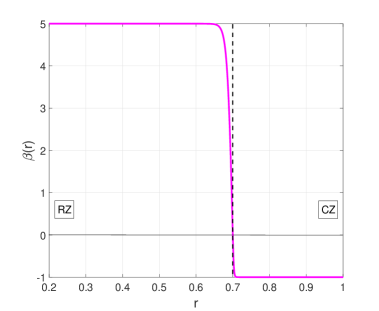
By selecting a suitable profile for (implicitly selecting an appropriate as described above) we can create a convectively stable region for and an unstable region for . Here, we choose the same prescription for the function as in Korre et al. (2019), namely
| (16) |
where is the stiffness parameter which measures the relative stability of the radiative zone to the convection zone and where and define the transition width between the two zones (see Figure 1). Since and its derivative must be continuous at , then . The function can also be interpreted as (minus) the ratio of the local Rayleigh number Ra to the global Rayleigh number Rao, i.e.
| (17) |
where
| (18) |
The minus sign in Equation (18) ensures that Ra is positive in convective regions. The presence of the magnetic field introduces the magnetic Prandtl number
| (19) |
and the Chandrasekhar number
| (20) |
which characterizes the relative importance of the Lorentz force to the viscous force.
In order to study the dynamics of the interaction of the overshooting motions with an initially contained dipolar magnetic field in the RZ, we have run 3D DNS solving the MHD Boussinesq equations in a spherical shell exactly as outlined above using the PARODY code (Dormy, Cardin & Jault, 1998; Aubert, Aurnou & Wicht, 2008). The chosen boundary conditions for the temperature translate to a no-flux boundary condition for the perturbations at the inner boundary, , and a zero temperature perturbation boundary condition at the outer boundary, . We employ stress-free boundary conditions for the velocity. For the magnetic field, we assume an electrically insulating outer boundary and a conducting inner core.
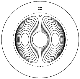
We initialize the MHD simulations from the corresponding purely hydrodynamic simulations (see Korre et al., 2019) that were evolved from a zero initial velocity and small-amplitude temperature perturbations until a statistically-stationary and thermally-relaxed state was achieved111We look both at the total kinetic energy per unit volume in the domain, (where is the volume of the spherical shell) and at the gradient of the temperature perturbations at the surface to check when that occurs.. We then start the MHD simulation from the end of the thermally-equilibrated hydrodynamic one, and initialize it with a purely poloidal dipole magnetic field initially contained in the stable zone below (Figure 2) of the form:
| (21) |
The parameter is simply a geometric factor chosen to guarantee that at . To ensure this, (where is the first root of the function , where is the Bessel function of order ).
All of the simulations reported here are for a fixed stiffness parameter , a transition width 222We note that in Korre et al. (2019), we presented a suite of numerical simulations of overshooting convection (ignoring the effect of magnetism and rotation) where we varied both and and studied the dependence of the overshooting dynamics on these input parameters. , Pr and Pm. We also fix the Chandrasekhar number to be equal to , indicating that the initial magnetic field is relatively weak. Note that the numerically achievable values of the Prandtl number and the Rayleigh number are not astrophysically realistic (e.g. for the Sun: Pr in the solar tachocline, and Ra) due to the computational constraints arising from the required spatial and temporal resolution of the simulations. However, the magnetic Prandtl number Pm is of the order of the solar value, which is approximately equal to Pm at the bottom of the solar CZ.
With these chosen parameters, there is no dynamo action, hence the field can only decay. In this paper, we focus solely on studying how the overshooting turbulent motions can affect the transport and overall evolution of a weak magnetic field. We vary Rao over three orders of magnitude (Ra, , , and ), and study the time-dependent evolution of the magnetic field as each simulation proceeds.
| Rao | Rm | ||||||
|---|---|---|---|---|---|---|---|
| 300 | 192 | 192 | 0.13 | 145 | 8 | ||
| 400 | 288 | 320 | 0.094 | 191 | 22 | ||
| 585 | 516 | 640 | 0.069 | 243 | 50 | ||
| 585 | 516 | 640 | 0.049 | 319 | 112 |
3 Numerical results
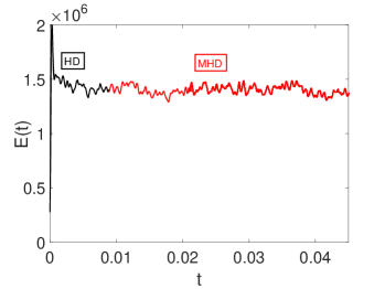
We begin by exploring the dynamics observed in a typical simulation with Ra. In Figure 3, we present the total kinetic energy per unit volume against time . The black line corresponds to from the purely hydrodynamic run (HD) from which the MHD simulation was restarted, while the red line is from the same simulation after adding the magnetic field (MHD). The kinetic energy does not change noticeably between the HD run and the MHD run, indicating that the inclusion of the field does not affect the convective dynamics significantly. This is expected since the field is initially weak, and decays with time. In Figure 4, we present snapshots of the radial velocity . In each panel, the left hemisphere shows the velocity field on a spherical shell close to the upper boundary at , illustrating the convective motions near the surface. The right hemisphere is a meridional slice showing the radial velocity for a selected longitude as a function of and at a) Ra, b) Ra, c) Ra and d) Ra taken during the statistically stationary state. In all cases, we notice that the degree of turbulence in the CZ increases with increasing Rao with higher Rayleigh numbers resulting in stronger eddies with a wider range of scales. Also, in the right hemispheres, we see that the convective motions generated within the convective region overshoot some distance beyond the bottom of the CZ (represented by the inner black line).
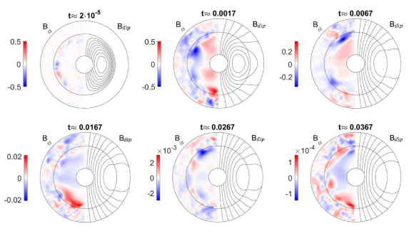
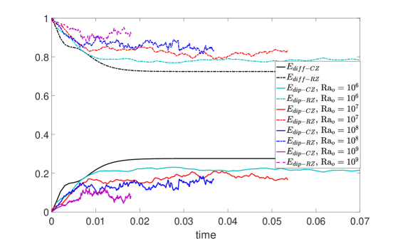
To illustrate the evolving geometry of the large-scale magnetic field, we plot contours of the dipole component of the poloidal field along with the azimuthally-averaged toroidal component of the magnetic field at Ra at different representative times (Fig. 5). The first panel shows the solution very close to the initial condition, where most of the dipole is still contained compactly within . At , the field has already diffused outwards a little, come into contact with the overshooting motions, and started “opening up" into the CZ. By , all of the field lines have now opened up into the CZ. This leads to the appearance of an unconfined configuration, i.e. a state where the dipole field lines have infiltrated the CZ substantially leaving very few (if any) closed field lines in the RZ. Note how the overall field geometry then barely changes after this point, suggesting that it may have settled into a particular eigenmode of the induction equation. The field amplitude is still decaying with time, however. At , is of order unity, but decreases by three orders of magnitude by the time .

We now analyze more quantitatively the results of the simulations, in order to get a better understanding of the spatio-temporal evolution of the field. In what follows, it will be informative to compare our numerical results to a hypothetical case without convection, in which the initial field merely diffuses away. In the absence of any fluid motion, the initial magnetic field evolves with time according to
| (22) |
with Pm. We can solve this equation semi-analytically, to compute the evolution of the magnetic energy in the absence of convection (see Appendix A). In Figure 6, we compare the volume average of the magnetic energy of the purely diffusive case along with the same quantity computed in the fully nonlinear convective simulation. Note that the dipole component of the magnetic field is given by
| (23) |
where
| (24) |
and , where is the amplitude of the dipole evolved in the code and is the spherical harmonic with degree corresponding to that dipole mode. Then, we define the spherically-averaged dipole magnetic energy in the simulation as
| (25) |
such that the volume-averaged dipole magnetic energy in the spherical shell is
| (26) |
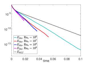
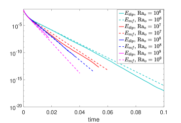
In Figure 6, we see that the evolution of the magnetic energy in the dipole field in the simulation coincides more or less with that of the purely diffusive solution (defined similarly to , but with replaced by ) for , but as time evolves beyond this point, begins to decrease much faster than . Notably, the decrease is faster for higher values of Rao. Furthermore, we notice that after some adjustment period, decays exponentially with a well-defined, constant decay rate (that depends on Rao). This confirms our conclusions from the visual inspection of Figure 5, and demonstrates that the dipole field in each simulation eventually settles into an eigenmode of the induction equation. This is consistent with the fact that the field is weak (so the Lorentz force in the momentum equation is negligible), so the induction equation is essentially kinematic (linear in ).
One could rightfully ask whether this significant and rapid loss of energy in the dipole (compared with the purely diffusive case) could potentially be attributed to Tayler instabilities. Past studies (e.g. Markey & Tayler, 1973; Wright, 1973; Spruit, 1999; Braithwaite, 2009) have shown that a purely poloidal field with closed field lines within a stable radiative zone is unstable to non-axisymmetric perturbations, and these MHD instabilities can lead to a substantial reduction of the magnetic energy. However, we do not observe any such instability in this work, because our initial field is too weak. Indeed, Tayler instabilities grow on an Alfvénic time-scale, which is for the parameter selected in this set of simulations. This is clearly longer than both the magnetic diffusion time-scale and the thermal diffusion time-scale in our system, which are and respectively. This, and the fact that the decay rate depends on Rao, lead us to the conclusion that the faster-than-diffusive decay is a consequence of the convective motions acting on the field, rather than other types of instabilities within the radiative zone.
Another quantitative way of examining the evolution of the initial field is to look at the radial distribution of the magnetic energy over time between the CZ and the RZ and compare it with the purely diffusive case. We define the fractional magnetic energy of the dipole in the RZ, , and in the CZ, , respectively, as
| (27) |
and
| (28) |
In Figure 7, we plot and versus time, for the runs with Ra as well as for the purely diffusive case, where we calculate and in a similar way.
At , the magnetic field is fully confined in the RZ, so and . As increases, we see that in all cases (both purely diffusive and the numerical simulations at increasing Rao), there is an initial decrease in and a concurrent increase in , which corresponds to the initial stages of the evolution where the dipole field begins to diffuse into the convection zone. Around , the purely diffusive case starts relaxing towards the slowest-decaying radial eigenmode of the diffusion equation, and eventually and asymptote to two constants with , indicating that the magnetic energy distribution is then decreasing self-similarly. The same general stages of evolution are seen in the DNS. The fractional energies of the full 3D calculations also asymptote to two statistically-stationary constants at each Rao, which confirms that the dipole field in each simulation has relaxed to the slowest decaying eigenmode of the induction equation. This is consistent with our findings that the dipole energy is decreasing exponentially in Figure 6. Crucially, however, we find that the ratio increases substantially with Rao, which could be interpreted as the field being increasingly more contained and therefore “confined" in the RZ than in the diffusive case.
In an effort to understand this behaviour, we now focus on the Ra case for which is the largest and begin by comparing the properties of its dipole eigenmode to that of the Ra case. We extract this eigenmode by computing the weighted time-average as
| (29) |
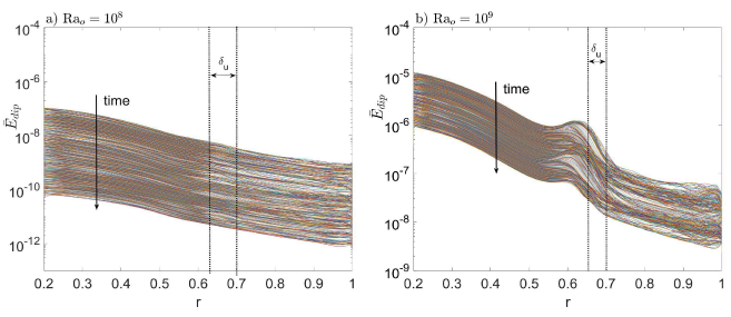
where is the number of available snapshots of the DNS at different times after (i.e. in the exponential decay phase), and where is the amplitude of the radial component of the dipole field at the inner boundary () at the pole, used here to normalize the decaying eigenmode. Figures 8a and 8b show selected field lines of for the Ra and Ra cases, respectively. In both cases, we see that the field lines have clearly diffused into the CZ. However, while all field lines are clearly open in the Ra case, some of the field lines appear to remain closed in the RZ in the Ra case, showing further evidence for a more confined state at higher Rao (in an average sense).
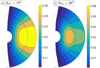
Figure 9a and Figure 9b compare more quantitatively the evolution of the dipole fields in the Ra and simulations, by showing as a function of radius at different times after the transient state. We see that for the Ra case, monotonically decreases from the RZ outward and decays with time. For the Ra run, by contrast, we observe a “bump" representing an excess of dipole energy that can be shown to be located just below the convective overshoot region. Indeed, as shown by Korre et al. (2019), it is possible to characterize the overshoot depth using the stopping distance of the strongest downflows originating from the CZ. The accumulation of the dipole energy in Fig. 9b appears to reside just below the radius . This suggests that it is likely associated with the ejection of the field from the CZ by the stronger downflows, akin to earlier ideas of “magnetic pumping" (e.g. Tobias et al., 1998, 2001). This effect does not appear to be significant at lower Rao and only appears here at Ra, supporting the notion that there must be a substantial change in the interaction between the magnetic field and the convective motions at the highest Ra case.
4 A mean-field model for the dynamics
The two effects found above – the increasingly rapid decay of the dipole field, and the increasing fraction of dipole magnetic energy in the RZ with increasing Rao – are inevitably due to induction effects. Much work has been done to characterize and classify the behaviour of the e.m.f. term using a mean-field approach, as described in the introduction. We have found that a mean-field model that includes both a magnetic pumping term (typically called a effect) and a turbulent diffusion term (typically called a effect) appears to be sufficient to correctly capture the effects of the turbulent flow on the mean field. We therefore now attempt to discern the effect of each one of these processes on the dipole field and their dependence on Rao.
The mean field induction equation for the large-scale field (where is an azimuthal average to distinguish between large scales of interest and small-scale turbulent motions), with these terms, is given by
| (30) |
where is the well-known “ effect" that is derived from the symmetric part of the mean-field tensor and allows the regeneration of large-scale poloidal magnetic fields, is derived from the antisymmetric part of the mean-field tensor and is related to the concept of magnetic pumping since looks like a velocity, and is associated with turbulent diffusion, where (often termed ) is the turbulent diffusivity. Even though the convection is not isotropic, we make the further approximation that , derived for 3D nearly isotropic turbulence (Krause & Raedler, 1980; Kichatinov & Rüdiger, 1992; Kitchatinov & Rüdiger, 2008).
Although Eq. (30) is usually written for any “mean-field", in what follows we take to be . Then, as before, we define to be the potential field such that , with
| (31) |
and thus obtain an evolution equation for ,
| (32) |
Projecting Eq. (32) onto the direction while also assuming that , i.e. that the turbulent diffusivity only has a radial dependence, and substituting the ansatz (31) then yields
| (33) |
where is the effective diffusivity (which is the sum of the microscopic diffusivity equal to Pm and the turbulent diffusivity). Once the simulation has reached the exponentially decaying eigenstate discussed earlier, we can assume that , where is the measured decay rate of the amplitude of the dipole in the exponential decay phase (see Table 1). Then, with a few algebraic manipulations we obtain
| (34) |
This equation can be used to infer the quantity , given and extracted from the DNS. However, the profiles of at individual time-steps are too noisy, and so cannot be used “as is". We therefore first perform a weighted time-average of in the exponentially decaying phase, as
| (35) |
where
| (36) |
This effectively extracts the eigenmode of the problem, as we did in Eq. (29) for . Now, let Then Eq. (34) becomes
| (37) |
which is a first-order ordinary differential equation for , given . Note that the problem is singular at the point where . However, the equation does have a regular solution, which we compute by enforcing the internal boundary condition
| (38) |
at that point, and numerically integrating Eq. (37) inward for and outward for . Profiles of obtained in this manner are shown and discussed below.
In order to cross-check the validity of the procedure, after computing we also solve the forward mean-field problem
| (39) |
subject to the same initial and boundary conditions on the field as in the DNS. In Figure 10, we plot the volume average of the dipole magnetic energy against the time for the four Ra cases from our DNS (solid lines) along with the dipole magnetic energy of the mean-field forward problem computed by using Eq. (39). We observe that, beyond the initial transient phase, the mean-field solution is quite close to the one calculated from the DNS in all of the cases and certainly acquires the correct decay rate. This serves as a validation of this approach.
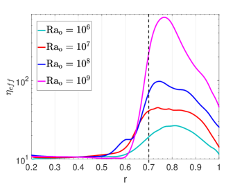
With this mean-field framework, we can now shed light on the effect of turbulent convection on the large-scale dipole field in terms of two mean-field effects – a pumping effect() and a turbulent diffusion effect () – and try to establish how these depend on Rao. Figure 11 shows the enhanced turbulent diffusivity in the bulk of the CZ and in the overshoot region due to the stronger turbulent convective motions there. We see values significantly enhanced from the microscopic value of everywhere except in the RZ, and generally increasing with Rao. These profiles strongly suggest that the dipole magnetic energy in the DNS decays faster than in the purely diffusive case due to an enhanced turbulent diffusivity in the CZ that increases with Rao.
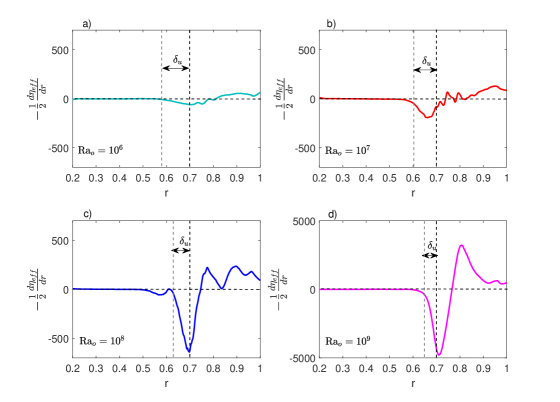
In Figure 12, we plot the term . This term can be interpreted as the diamagnetic velocity that transports the dipole magnetic field down the gradient of turbulent intensity, from the highly turbulent regions (i.e. the CZ and the overshoot region) into the stable RZ below. Consistent with the gradients seen in Fig. 11, we find that this pumping term increases in magnitude with increasing Rao, is maximal close to the bottom of the CZ and drops to zero again outside of the overshoot layer (marked in the figure with the length-scale ).
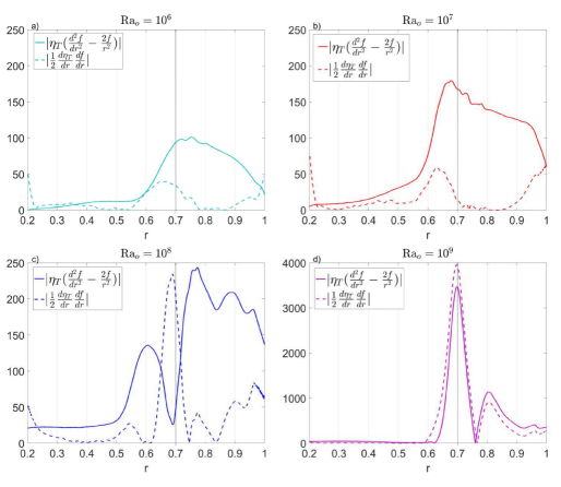
To understand the relative importance of pumping (which transports the field inward) and turbulent diffusion (which transports the field outward) in each case, in Figure 13, we plot the magnitude of the full terms associated with the magnetic pumping and the turbulent diffusion , respectively, for the four values of the Rayleigh number. Both of these terms increase with increasing Rao as expected. For Ra and Ra turbulent diffusion is larger than magnetic pumping. At Ra, the pumping term localized in the overshoot region becomes as strong as the maximum bulk turbulent diffusion. At Ra, the behaviour in the overshoot zone dominates both terms, and the pumping term has finally exceeded the turbulent diffusion term. This can explain what we observe in Fig. 9b, namely that magnetic pumping is efficient enough to lead to the accumulation of the dipole field within and below the overshoot region.
5 Discussion
5.1 Discussion of the results
In this work, we used DNS to elucidate the dynamical interaction of overshooting convection with underlying magnetic fields. To understand the dynamics found in our simulations more intuitively, we compared our results to a mean-field model that contains both a turbulent diffusivity and a pumping term related to the gradient of the turbulent diffusivity. From this comparison, we were able to extract the turbulent diffusivity profile . Solving the forward mean-field problem (given in Eq. (39) subject to the same initial and boundary conditions as those used in the DNS) confirmed that this mean-field approach indeed predicts reasonably well the overall decay rates of the magnetic field observed in the DNS results. The fact that this model works reasonably well is perhaps somewhat surprising, since it makes the simplistic assumption that the transport velocity (given by ) is derived from nearly isotropic turbulence, which is certainly not the case for convection.
For this model to be useful as a predictive tool, it is necessary to understand the dependence of the turbulent diffusivity that underpins the model on parameters that might be known for stellar interiors. Here we have kept the Prandtl number constant so our main concern is the dependence on the Rayleigh number. For that purpose, in Figure 14, we plot the values of (with their error bars – see Appendix B for more details) against Rao, where we define as
| (40) |
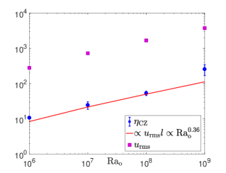
Since the Lorentz force is negligible, from a dimensional perspective we expect that should scale as Rm/Pm (see, e.g. Cattaneo & Vainshtein, 1991), where is the non-dimensional rms velocity of the fluid extracted from the DNS, is the depth of the CZ, and Rm is the magnetic Reynolds number (see Table 1) defined in terms of non-dimensional quantities as
| (41) |
We find that this scaling holds for the three lower Rao cases but not for the Ra simulation, even taking into account the errors in the measurement. The fact that the highest Rao case deviates from this scaling could be attributed to two main possible reasons. First, it could be that the mean-field model is indeed a reasonable model of the fully nonlinear dynamics, but the correlations between the convection and the field that lead to have actually changed. Second, it could be that the simplistic mean-field model adopted here fails at higher Rao, omitting some dynamics that become important. For example, the use of Eq. (30) to model is derived from nearly isotropic turbulence, and may become incorrect, or other anisotropic elements of the original tensor may become important. Fitting of an incorrect mean-field model would in this case lead to inaccurate values of that do not follow the expected scaling in Figure 14. In either case, the mismatch of the mean-field model and our numerical results appears to indicate a substantial change in the dynamics at Ra. It is important to further explore this new dynamical regime beyond Ra, but unfortunately this is presently not possible with PARODY due to computational constraints.
5.2 Implications for magnetic confinement and decay of the large-scale dipole field in the RZ
Overall, our numerical results suggest that there is an increasing degree of “confinement" of the dipole field to the stable RZ as the Rayleigh number increases, with a regime change around Ra, as described above. It is important to note that the confinement mechanism here is very different from that described theoretically by Gough & McIntyre (1998) and exhibited in the models of Acevedo-Arreguin et al. (2013) and Wood & Brummell (2018). In these models, the confining mechanism depends crucially on the presence of global rotation and is a slow, laminar process operating via large-scale meridional flows. Confinement is then viewed as a balance between downward advection and upward diffusion (see Section 1). In our 3D simulations, which are without any rotation, there are no large-scale meridional flows and instead the confinement is achieved on a rapid advective time-scale by a balance between upward turbulent diffusion, and downward turbulent pumping. At the highest value of Rao achieved, the pumping is becoming sufficient to create a relatively confined state. These results are very similar to what was found in Tobias et al. (2001) and in Tao et al. (1998) who both studied turbulent transport of a mean-field in a Cartesian geometry via 3D and 2D numerical simulations, respectively. Tobias et al. (2001) performed a quantitative survey of the effect of on the turbulent pumping of the magnetic field by varying over five orders of magnitude. They concluded that their results were very insensitive to this parameter. Tao et al. (1998) found that in the kinematic regime where the magnetic field is weak, the kinematic mean-field model works remarkably well in predicting the expulsion process of the field while they concluded that, in the dynamical regime, turbulent transport still takes place although not so efficiently as in the kinematic regime due to suppression of the effective turbulent diffusivity. Therefore, following these prior studies indicating that there is overall little dependence of the dynamics on , we examined a low value of to give this study the best chance of obtaining turbulent pumping, bearing in mind that we could explore the computationally harder dynamical regime in a future study given the necessary but currently not available computational resources. Also, our explanation in terms of mean-field theory is very similar to that which was proposed by Kitchatinov & Rüdiger (2008). In that paper, only the forward problem was solved with an profile parametrised using an error function, transitioning between a high value in the CZ given by and a much lower value in the RZ given by . Despite the fact that the profile is quite different from the one we derive in our simulations, Kitchatinov & Rüdiger (2008) also reported that poloidal field lines start to become confined at values of , which is commensurate with what we have for Ra. Kitchatinov & Rüdiger (2008) report greater confinement at much higher ratios , pointing to the tantalising need for simulations at higher Rao. Based on their results, we might need to be larger than what we currently have to obtain a more confined field in the RZ. Assuming that the traditional scaling of , with , still holds, this would require a Rayleigh number that is times larger than the highest Rayleigh case we were able to simulate.
It is possible that some factors may mitigate this issue however. For example, it has long been suggested that topology can play a significant role in pumping (Drobyshevski & Yuferev, 1974). The simulations of Tobias et al. (2001) that showed relatively efficient pumping were carried out at only moderate Rayleigh numbers () but were performed in a compressible fluid, where there is significant asymmetry in the convection. Switching to more naturally asymmetric anelastic or compressible turbulence may enhance turbulent pumping.
It should be highlighted, as it was in Tobias et al. (2001) and found here, that pumping acts on large-scale (i.e. significantly larger than the advective scales) magnetic fields only. As such, there may be significant fluctuations in the field leading to a significant magnetic energy , remaining in the overshoot layer, even though the mean field is confined below it. Similarly, small-scale magnetic fields (at the velocity scales or smaller) are constantly recirculating in the convection zone so the latter is by no means free of magnetic energy.
Finally, note that our data suggest that the decay rate () of the dipole field increases with increasing . However, in far more turbulent cases (where the confinement would be more efficient), we would expect that the decay rate of the large-scale dipole field would depend less on what happened in the convective region and more on the conditions within the CZ-RZ interface and the RZ, which would need to be modeled (although how remains to be determined).
6 Conclusion and astrophysical implications
Our results suggest that solar-type stars with masses , which have thick convective envelopes with extremely large Rao, could possess primordial dipole magnetic fields that are fully confined in their stable region. By contrast, Rao rapidly decreases in higher-mass solar-type stars with thinner outer convective regions, and are therefore less turbulent, and as a result, a mean poloidal field may not be able to remain confined in their RZ.
We have discussed two different possible mechanisms for confinement, namely the turbulent confinement process associated with convective overshooting motions operating on fast time-scales (studied in this paper) and the laminar confinement associated with slow, rotationally-driven meridional motions. It is very likely that both of these confinement processes will play a role in the solar tachocline, where it has been shown that the presence of a confined poloidal field in the stable region is needed to explain simultaneously the uniform rotation of the RZ and the thinness of the tachocline (see, e.g. Gough & McIntyre, 1998). Also, it is not unlikely that a model similar to the Gough & McIntyre (1998) model may be able to account for the dynamical coupling of the core and envelope of RGB stars (e.g. Mosser et al., 2012).
As discussed above, turbulent transport processes taking place in these stars can only lead to the confinement of their large-scale field and small-scale fields will still be present in both the overshoot region and the convection zone, either as in these simulations, or by dynamo action. Hence, it would be interesting to understand whether Ferraro’s isorotation theorem can still persist in the same way under these more complicated conditions. Also, it is important to obtain better estimates of the amplitude of the small-scale field residing in the tachocline. If this small-scale field is strong enough, it can significantly impact the conclusions of the Gough & McIntyre (1998) model which assumes a magnetic-free tachocline.
Ultimately, our findings and conclusions suggest that it is of paramount importance to now focus on the effects of the small-scale dynamo field existing in the vicinity of the CZ-RZ interface and understand its influence on the interior dynamics as it infiltrates the stable radiative zone from above. These ideas will be further investigated in the upcoming paper II of this series of papers.
Acknowledgements
The authors thank Toby Wood for fruitful discussions. L.K. acknowledges support from the George Ellery Hale Post-Doctoral Fellowship and from National Aeronautics and Space Administration (NASA) grant No. 80NSSC17K0008. C.G. acknowledges support from the UK Natural Environment Research Council grant NE/M017893/1. This work was also partially supported by National Aeronautics and Space Administration (NASA) Grant No. 80NSSC20K0602 (sub-award 62356550-145590). The authors acknowledge the Texas Advanced Computing Center (TACC) at The University of Texas at Austin for providing HPC resources that have contributed to the research results reported within this paper (URL: http://www.tacc.utexas.edu). The initial hydrodynamic simulations were run on the Hyades cluster at the University of California, Santa Cruz, purchased using the National Science Foundation (NSF) grant No. AST-1229745.
Data Availability
The data underlying this article will be shared on reasonable request to the corresponding author. The PARODY-JA code is maintained by Julien Aubert and can be obtained upon request (http://www.ipgp.fr/~aubert/Julien_Aubert,_Geodynamo,_IPG_Paris/Software.html).
References
- Acevedo-Arreguin et al. (2013) Acevedo-Arreguin L. A., Garaud P., Wood T. S., 2013, MNRAS, 434, 720
- Aerts et al. (2019) Aerts C., Mathis S., Rogers T. M., 2019, ARA&A, 57, 35
- Aubert et al. (2008) Aubert J., Aurnou J., Wicht J., 2008, Geophysical Journal International, 172, 945
- Beck et al. (2012) Beck P. G., et al., 2012, Nature, 481, 55
- Braithwaite (2009) Braithwaite J., 2009, Monthly Notices of the Royal Astronomical Society, 397, 763
- Brun & Zahn (2006) Brun A. S., Zahn J. P., 2006, A&A, 457, 665
- Cattaneo & Vainshtein (1991) Cattaneo F., Vainshtein S. I., 1991, ApJ, 376, L21
- Chandrasekhar (1956) Chandrasekhar S., 1956, Astrophysical Journal, 124, 244
- Charbonneau & MacGregor (1993) Charbonneau P., MacGregor K. B., 1993, ApJ, 417, 762
- Donati & Landstreet (2009) Donati J. F., Landstreet J. D., 2009, ARA&A, 47, 333
- Dormy et al. (1998) Dormy E., Cardin P., Jault D., 1998, Earth and Planetary Science Letters, 160, 15
- Drobyshevski & Yuferev (1974) Drobyshevski E. M., Yuferev V. S., 1974, Journal of Fluid Mechanics, 65, 33
- Ferraro (1937) Ferraro V. C. A., 1937, MNRAS, 97, 458
- Garaud (1999) Garaud P., 1999, Monthly Notices of the Royal Astronomical Society, 304, 583
- Garaud & Rogers (2007) Garaud P., Rogers T., 2007, in Stancliffe R. J., Houdek G., Martin R. G., Tout C. A., eds, American Institute of Physics Conference Series Vol. 948, Unsolved Problems in Stellar Physics: A Conference in Honor of Douglas Gough. pp 237–248
- Gough & McIntyre (1998) Gough D. O., McIntyre M. E., 1998, Nature, 394, 755
- Gough et al. (1996) Gough D. O., et al., 1996, Science, 272, 1296
- Irwin et al. (2007) Irwin J., Hodgkin S., Aigrain S., Hebb L., Bouvier J., Clarke C., Moraux E., Bramich D. M., 2007, MNRAS, 377, 741
- Kichatinov & Rüdiger (1992) Kichatinov L. L., Rüdiger G., 1992, A&A, 260, 494
- Kitchatinov & Rüdiger (2008) Kitchatinov L. L., Rüdiger G., 2008, Astronomische Nachrichten, 329, 372
- Korre et al. (2017) Korre L., Brummell N., Garaud P., 2017, Phys. Rev. E, 96, 033104
- Korre et al. (2019) Korre L., Garaud P., Brummell N. H., 2019, MNRAS, 484, 1220
- Krause & Raedler (1980) Krause F., Raedler K. H., 1980, Mean-field magnetohydrodynamics and dynamo theory
- MacGregor & Charbonneau (1999) MacGregor K. B., Charbonneau P., 1999, ApJ, 519, 911
- Markey & Tayler (1973) Markey P., Tayler R. J., 1973, Monthly Notices of the Royal Astronomical Society, 163, 77
- Marques et al. (2013) Marques J. P., et al., 2013, A&A, 549, A74
- Mestel (1999) Mestel L., 1999, Stellar magnetism
- Mestel & Weiss (1987) Mestel L., Weiss N. O., 1987, MNRAS, 226, 123
- Mosser et al. (2012) Mosser B., et al., 2012, A&A, 548, A10
- Oglethorpe & Garaud (2013) Oglethorpe R. L. F., Garaud P., 2013, ApJ, 778, 166
- Rüdiger & Kitchatinov (1997) Rüdiger G., Kitchatinov L. L., 1997, Astronomische Nachrichten, 318, 273
- Spiegel & Veronis (1960) Spiegel E. A., Veronis G., 1960, ApJ, 131, 442
- Spruit (1999) Spruit H. C., 1999, A&A, 349, 189
- Strugarek et al. (2011) Strugarek A., Brun A. S., Zahn J. P., 2011, A&A, 532, A34
- Tao et al. (1998) Tao L., Proctor M. R. E., Weiss N. O., 1998, MNRAS, 300, 907
- Tobias et al. (1998) Tobias S. M., Brummell N. H., Clune T. L., Toomre J., 1998, ApJ, 502, L177
- Tobias et al. (2001) Tobias S. M., Brummell N. H., Clune T. L., Toomre J., 2001, ApJ, 549, 1183
- Weiss (1966) Weiss N. O., 1966, Proceedings of the Royal Society of London Series A, 293, 310
- Wood & Brummell (2018) Wood T. S., Brummell N. H., 2018, ApJ, 853, 97
- Wood & McIntyre (2011) Wood T. S., McIntyre M. E., 2011, Journal of Fluid Mechanics, 677, 445
- Wood et al. (2011) Wood T. S., McCaslin J. O., Garaud P., 2011, ApJ, 738, 47
- Wright (1973) Wright G. A. E., 1973, Monthly Notices of the Royal Astronomical Society, 162, 339
Appendix A SOLUTION OF THE DIFFUSION EQUATION
In this appendix, we derive the solution of the diffusion equation for the poloidal axisymmetric magnetic field given by
| (42) |
where could be a function of . Following the work of Chandrasekhar (1956), we can express in terms of the potential such that
| (43) |
Substituting Eq. (43) into Eq. (42) yields
| (44) |
where .
We seek separable solutions of the form
so Eq. (44) yields separate equations for and :
| (45) |
and
| (46) |
Equation (46) is the eigenvalue equation of the Gegenbauer polynomial , with the eigenvalues given by , where .
Hence, the full solution is given by (see Garaud, 1999)
| (47) |
If we focus on the dipole configuration, the only coefficient that is non-zero is for . The corresponding polynomial is simply , with . The remaining equation for (Eq. (45)) is:
| (48) |
The boundary conditions require that and be continuous at , and that there is no singularity at the origin , i.e. finite. Solutions of Eq. (48) with these conditions are Bessel functions of fractional order.
The solution for is then given by
| (49) |
where is the Bessel function of order , and where the coefficient is given by
| (50) |
Finally, the field components can be written in terms of (see Eq. (43)) as
| (51) |
Appendix B CALCULATION OF ERRORBARS FOR
For the calculation of , we calculate the weighted-average (see Eq. (35)) from available snapshots of the DNS at different times in the exponential decay phase. In order to obtain errorbars for , we split the snapshots into subsets, each consisting of fewer than snapshots. Each one of these subsets of snapshots corresponds to a time interval within the exponential decay phase of the simulation. We chose to ensure that contains many convective turnover time-scales and more than one turbulent diffusion time-scale, in order for the calculated error to be physically reasonable.
Following the same process as described in Section 4 for the calculation of , we obtain a profile of in each individual subset ().
From that, we then calculate as
| (52) |
Finally, the errorbar for can be found by using Eq. (40) where we have replaced with .