The infancy of core-collapse supernova remnants

Abstract

We present 3D hydrodynamic simulations of neutrino-driven supernovae (SNe) with the Prometheus-HotB code, evolving the asymmetrically expanding ejecta from shock breakout until they reach the homologous expansion phase after roughly one year. Our calculations continue the simulations for two red supergiant (RSG) and two blue supergiant (BSG) progenitors by Wongwathanarat et al., who investigated the growth of explosion asymmetries produced by hydrodynamic instabilities during the first second of the explosion and their later fragmentation by Rayleigh-Taylor instabilities. We focus on the late time acceleration and inflation of the ejecta caused by the heating due to the radioactive decay of ⁵⁶Ni to ⁵⁶Fe and by a new outward-moving shock, which forms when the reverse shock from the He/H-shell interface compresses the central part of the ejecta. The mean velocities of the iron-rich ejecta increase between 100 km/s and 350 km/s ($\sim$8–30%), and the fastest one percent of the iron accelerates by up to $\sim$1000 km/s ($\sim$20–25%). This ‘Ni-bubble effect’, known from 1D models, accelerates the bulk of the nickel in our 3D models and causes an inflation of the initially overdense Ni-rich clumps, which leads to underdense, extended fingers, enveloped by overdense skins of compressed surrounding matter. We also provide volume and surface filling factors as well as a spherical harmonics analysis to characterize the spectrum of Ni-clump sizes quantitatively. Three of our four models give volume filling factors larger than $0.3$, consistent with what is suggested for SN 1987A by observations.

1 Introduction

Core-collapse supernova (CCSN) explosions are the most violent phenomena that happen at the end of the lifetime of massive stars. They shed light onto extreme physical conditions and processes inside the exploding star, which otherwise are inaccessible by observations in the electromagnetic spectrum. Despite the significant progress of our theoretical understanding of these events due to the feasibility of three-dimensional (3D) simulations, answering the question whether the explosion is driven by the delayed neutrino-heating mechanism still requires further studies and, in particular, observational assessment in direct comparison to 3D model predictions. Therefore, it is of great importance to determine possibilities of testing the consequences of the explosion mechanism with detailed observations. Promising objects for this kind of observations are young SN remnants (SNR), which still carry the imprints of explosion asymmetries reflected by the 3D spatial distributions of different chemical elements synthesized during the SN outburst.

In particular, observations of SN 1987A in the Large Magellanic Cloud and Cassiopeia A (Cas A), a $\sim 340$ year old galactic SNR, offer possibilities to indirectly probe the CCSN mechanism. The explosions producing these two fascinating objects must have been of genuine 3D nature, as already expected by extensive theoretical studies, and as suggested by abundant observational evidence gathered over the past decades. For instance, Larsson et al. (2016) inferred the 3D distribution of the ejecta of SN 1987A by using Doppler shift information of the velocities of different elements obtained from spectroscopic observations. The analysis showed global large-scale asymmetries of the SN ejecta extending along the northeast and the southwest directions. DeLaney et al. (2010) reconstructed the 3D ejecta structure of Cas A using observational data obtained in infrared by the Spitzer Space Telescope (Isensee et al., 2010), in X-ray by the Chandra satellite (Lazendic et al., 2006), and in optical (Fesen & Gunderson, 1996; Fesen, 2001). The reconstruction revealed that the remnant can be characterized by a spherical component illuminated by the reverse shock, a flattened ejecta structure seen as a tilted thick disk, two opposing wide-angle, jet-like ejecta pistons, and numerous optical fast-moving knots lying in the thick disk plane. Spectroscopic observations of SN light echoes from SN 1987A (Sinnott et al., 2013) and Cas A (Rest et al., 2011) provide evidences that the observed large-scale ejecta asymmetries in these objects originate from very early phases of the explosions. In addition, direct observations of spectra and the lightcurve of SN 1987A show the presence of large scale anisotropies (Utrobin et al., 2015). Grefenstette et al. (2014) and Grefenstette et al. (2017) directly imaged the spatial distribution of radioactive ⁴⁴Ti in Cas A. They found strong hints that there must have been significant asymmetries during the explosion. Milisavljevic & Fesen (2013) and Milisavljevic & Fesen (2015) showed that the shocked ejecta strongly emitting in optical light are organized in ring-like structures that connect to the borders of seemingly empty bubbles or cavities in the interior of unshocked sulfur-rich ejecta. A comparison of recent Very Large Telescope/SINFONI observations of HII emission regions (Larsson et al., 2019) and Atacama Large Millimeter/Submillimeter Array (ALMA) observations of CO and SiO molecules and dust (Abellán et al., 2017; Cigan et al., 2019) shows that these molecules reside in different regions of the young supernova remnant.

On the theoretical side, there have been first successful attempts to model the observed structures of the ejecta in Cas A (Orlando et al., 2016) and of SN 1987A (Ono et al., 2020; Orlando et al., 2020a). However, the former models relied on a particular choice of the initial conditions at the shock breakout and the latter on parameterized initial explosion asphericities, both of which are not compatible with or would have to be checked against self-consistent calculations (Wongwathanarat et al., 2017).

In the context of neutrino-driven explosions, which we consider here, large-scale asymmetries originate from the nonlinear growth of hydrodynamic instabilities, as for example the convective instability (Bethe, 1990; Herant & Benz, 1992; Herant & Woosley, 1994; Burrows et al., 1995; Janka & Müller, 1995, 1996) and the standing accretion shock instability (SASI; Foglizzo, 2002; Blondin et al., 2003; Blondin & Mezzacappa, 2006; Ohnishi et al., 2006; Foglizzo et al., 2007; Scheck et al., 2008; Fernández, 2010), during the revival of the stalled SN shock wave. These asymmetries particularly manifest themselves in the distribution of the heavy elements, freshly synthesized during the explosion. After the revival of the shock wave, which takes less than $1$ s, the initial asymmetries get shaped further by the growth of secondary Rayleigh-Taylor instabilities (RTIs) that develop due to the propagation of the SN shock through the non-monotonically varying density gradients of the mantle and the envelope of the exploding progenitor star (Chevalier, 1976; Chevalier & Klein, 1978). Inspired by the SN 1987A event a large number of multi-D simulations studying the growth of RTIs at different composition shell interfaces (e.g. C+O/He and He/H interfaces) inside the progenitor star have been performed (e.g., Arnett et al., 1989; Müller et al., 1991b; Fryxell et al., 1991; Hachisu et al., 1990, 1992, 1994; Iwamoto et al., 1997; Nagataki et al., 1998; Hungerford et al., 2003, 2005; Joggerst et al., 2009; Joggerst et al., 2010b, a; Couch et al., 2009, 2011; Ono et al., 2013; Ellinger et al., 2012, 2013; Mao et al., 2015). However, these studies did not consistently model the development of explosion asymmetries introduced by convection and SASI during the first second of the explosion. To circumvent the underlying problem of a still uncertain CCSN explosion mechanism, these previous simulations either assumed spherical explosions or relied on asymmetric explosions with global, low-mode asymmetries imposed artificially. More recently, simulations of supernova explosions have been achieved with fully self-consistent calculations, where the shock revival was computed with detailed neutrino transport (Takiwaki et al., 2014; Melson et al., 2015b; Melson et al., 2015a; Lentz et al., 2015; Roberts et al., 2016; Summa et al., 2016; Müller et al., 2017, 2018; Vartanyan et al., 2018; Ott et al., 2018; O’Connor & Couch, 2018; Melson et al., 2020; Vartanyan et al., 2019; Burrows et al., 2019). Typically, these simulations stop after the shock wave is revived and starts to expand through the progenitor.

Long-time CCSN simulations which consider the explosion engine in multi-D and follow the time evolution of explosion asymmetries from the initiation of neutrino-driven explosions until late phases were carried out first in 2D by Kifonidis et al. (2003, 2006) and Gawryszczak et al. (2010), and more recently in 3D by Hammer et al. (2010), Wongwathanarat et al. (2013, 2015, 2017), and Stockinger et al. (2020). In these calculations, the emission of neutrinos by the nascent proto-neutron star (PNS) is parameterized and the interactions of these neutrinos with the post-shock matter are calculated by solving neutrino-transport equations with a grey approximation in a ray-by-ray manner (Scheck et al., 2006). The neutrino-matter interactions play a crucial role in reviving the stalled SN shock and in depositing the energy of the SN blast. With this approach it is not possible to determine all the properties of the involved neutrinos, whereas the growth of the hydrodynamic instabilities in the post-shock layer can be studied in most aspects realistically. These long-time CCSN simulations typically follow the propagation of the SN ejecta until hours or a day after the onset of the explosion. This is roughly the time at which the SN shock wave breaks out from the surface of the progenitor star. Müller et al. (2018) studied the explosion of an ultrastripped supernova and evolved their model until shock breakout.

After the SN shock breakout additional energy input from the radioactive decay of ⁵⁶Ni continues to drive inflation of ⁵⁶Ni-rich structures and facilitates mixing between ejecta components. This late time expansion can still lead to substantial modifications of the overall SN ejecta morphology on timescales of weeks or months (Benz et al., 1994). In 2D calculations and in calculations in a $30^{\circ}$ wedge of a 3D domain, Herant & Benz (1991, 1992) found that the energy input by radioactive $\beta$ decays can boost the ejected velocity of ⁵⁶Ni-rich clumps from $900\,$km/s to $1300\,$km/s and from $1400\,$km/s to $1900\,$km/s, corresponding to about a $30\%$ increase. A similar magnitude of the velocity increase was found by Basko (1994), who studied the growth of RTI at the surface of an inflating ⁵⁶Ni-rich bubble. With artificial initial setups, Blondin et al. (2001) studied how ⁵⁶Ni-rich clumps are heated and inflated by the radioactive decay energy and how they interact with the surrounding SN ejecta and the reverse shock. They confirmed previous expectations that the density along the borders of the ⁵⁶Ni-bubbles increases. The density contrast between these structures of overdense filaments, and the matter inside the ⁵⁶Ni-rich bubbles increases, because the latter reduces its density due to an additional expansion. The corresponding study was motivated by an analysis of observational data of SN 1987A carried out by Li et al. (1993), who provided an estimate of the filling factor of ⁵⁶Ni clumps of $f\gtrsim 0.3$ in the SN ejecta. In a 1D model considering either pure hydrodynamical or coupled radiation-hydrodynamical evolution, Wang (2005) found that during the inflation of a central spherical ⁵⁶Ni-bubble a dense shell of up to $1\,$M_⊙ is swept up, resulting in a maximal density enhancement of a factor of $100$ with respect to the ambient medium density. Such a ‘Ni bubble’ effect was also observed in recent 1D SN models with ⁵⁶Ni decay analyzed by Jerkstrand et al. (2018)

To follow the creation of the early-time SN ejecta asymmetries and their continuous transformation by secondary instabilities and by inflation caused by $\beta$-decay energy input, it is indispensable to perform 3D computer simulations. To capture the initial asymmetries consistently, these simulations have to start before the onset of the explosion and continue until the ejecta evolve into its gaseous remnant state. Such multi-physics, multi-scale simulations are computationally challenging and expensive. In this work, we continue the efforts by Wongwathanarat et al. (2015, 2017) to model the long-time evolution of CCSNe beyond the SN shock breakout until the early SNR phase roughly 1 year after the shock formation. We employ the models calculated by Wongwathanarat et al. (2015) as our initial data. In order to investigate the effect of radioactive heating on the SN ejecta asymmetries on a long timescale, we extend previous work by implementing a simplified treatment of the energy input due to the $\beta$ decay of ⁵⁶Ni and ⁴⁴Ti. Our approach is different from the one typically employed in other calculations (e.g., Herant & Benz, 1991, 1992), where energy deposition by the radioactive decay of ⁵⁶Ni is assumed to be local regardless of the optical depth of the ⁵⁶Ni-rich ejecta. Results from our 3D hydrodynamic calculations we present here have already been used in comparisons to 3D distributions of CO and SiO molecular emission in SN 1987A obtained recently by ALMA (Abellán et al., 2017; Cigan et al., 2019), for more realistic estimates of the X-ray absorption and emission in young CCSN remnants like Cas A and SN 1987A (Alp et al., 2018a, b, 2019; Jerkstrand et al., 2020), and in a geometrical analysis of the Fe distribution and neutron star kick in SN 1987A by Janka et al. (2017).

This paper is organized as follows. In Section 2, we briefly describe the numerical methods employed in our code. In addition, we explain in detail our approach to model the radioactive $\beta$-decay energy deposition and provide a brief overview of the properties of the considered progenitor models. In Section 3, we present results from our numerical models, beginning with the dynamics of a self-reflected reverse shock, the effect of $\beta$ decays on the global properties of the ejecta, a detailed view on the properties of the ejecta structures such as the velocity and density distributions, and finally the inflation of ⁵⁶Ni-rich clumps and their properties. We conclude and discuss our findings in Section 4. In Appendix A, we provide more details about our treatment of the $\beta$ decay.

2 Theoretical framework

2.1 Numerics

For our simulations we use the 3D, explicit finite-volume hydrodynamics code Prometheus (Fryxell et al., 1991; Müller et al., 1991b, a) in its version Prometheus-HotB (Janka & Müller, 1996; Kifonidis et al., 2003, 2006; Scheck et al., 2006; Arcones et al., 2007; Wongwathanarat et al., 2013, 2015, 2017; Gessner & Janka, 2018; Stockinger et al., 2020), which includes neutrino physics, a general equation of state applicable above and below nuclear statistical equilibrium, and a treatment of nuclear burning via a small alpha network. The hydrodynamics equations are solved with the piecewise parabolic method (PPM; Colella & Woodward, 1984) employing an exact Riemann solver for real gases (Colella & Glaz, 1985) and treating a multi-fluid system with the consistent multi-fluid advection (CMA) scheme by Plewa & Müller (1999). In our simulations, we consider a stellar fluid consisting of 19 nuclear species: protons, alpha nuclei from ⁴He to ⁵⁶Ni, ⁵⁶Co, ⁵⁶Fe, ⁴⁴Sc, ⁴⁴Ca, and a neutronization tracer X which traces production of neutron rich nuclear species when the electron fraction $Y_{e}<0.49$. The multi-dimensional Euler equations are solved in one-dimensional sweeps following the splitting technique of Strang (1968).

Spatial discretization of the computational sphere is done using an axis-free overlapping ‘Yin-Yang’ grid technique (Kageyama & Sato, 2004) implemented into Prometheus-HotB by Wongwathanarat et al. (2010). The Yin-Yang overset grid avoids numerical artefacts which can arise near the polar axis of a spherical polar grid. In addition, it also alleviates time step constraints imposed by the Courant-Friedrich-Levy (CFL) condition, which in the case of a spherical polar grid is very restrictive due to small azimuthal grid cells in the polar regions. Thus, the use of the Yin-Yang grid allows the simulations to advance with larger time steps.

As in Wongwathanarat et al. (2015), Newtonian self-gravity is taken into account by solving the integral form of Poisson’s equation with a multipole expansion method as described in Müller & Steinmetz (1995) and we omit the local relativistic corrections to the potential, which were included in Wongwathanarat et al. (2013), who calculated the early time evolution of the explosion of our models. The gravitational potential of the central point mass, which accounts for the gravitating effects of the neutron star (sitting far interior to our inner grid boundary) and includes monopole general-relativistic corrections, is treated continuously to avoid numerical transients, and it is updated during the simulation for mass leaving the inner grid boundary and assumed to be accreted by the neutron star.

At the late times considered here, the only remaining effect of neutrinos on the expanding ejecta is the waning neutrino-driven wind (i.e., a mass outflow from the nascent neutron star driven by neutrino-energy deposition), which is taken into account in the long-time simulations in a parametrized functional form that is prescribed as a boundary condition at the inner grid boundary. This is described in detail in Wongwathanarat et al. (2015), and already there the influence at the end of the simulation was negligible. For the details of the grey, ray-by-ray treatment of neutrinos applied in the early phases of the explosion (but not of relevance for the long-time simulations discussed in the present paper), we refer to Scheck et al. (2006) and Wongwathanarat et al. (2013, 2015).

At late phases, when the ejecta expand almost homologously, we move the grid radially as the SN ejecta expand. This moving mesh further relaxes the CFL condition imposed by grid cells with smallest radial extension, which are found at the smallest radii. The grid velocity is set to be linearly proportional to the radius, with the velocity of the outermost grid cell being set to $\sim 120\%$ of the maximal fluid velocity. The grid velocity of the inner radial grid boundary is forced to be zero, i.e. it remains at a fixed radius at all times. The shock may still expand faster than the maximum grid velocity. To avoid that the shock leaves the numerical grid during the simulations, we remove the innermost cell in radial direction and add a new cell in the exterior whenever the shock gets closer than 10 grid cells to the outer boundary of the computational domain. The physical conditions of the new grid cell are determined by the assumed stellar wind in the exterior. All other cell indices are shifted by minus one in radial direction, such that the previously second cell is now the first one. Since $|v_{r}|\gg\{|v_{\theta}|,|v_{\varphi}|\}$ the grid movement is quasi-Lagrangian and this treatment thus minimizes the numerical diffusion associated with the expansion of the SN ejecta over many orders of magnitude of the initial radial scale.

While, in general, we use an exact Riemann solver for ideal gases, we employ either the HLLE (Einfeldt, 1988) or the AUSM+ solver (Liou, 1996) inside grid cells where strong shocks are present in order to suppress numerical artefacts that can arise due to odd-even decoupling (Quirk, 1994). The more diffusive HLLE solver is used when the computational grid is expanding radially, while the AUSM+ solver is employed in the case of a static grid.

A previous version of the Prometheus-HotB code has already been applied to compute the propagation of the shock and the ejecta during a neutrino-driven supernova explosion up to the shock breakout in three dimensions and to study the production of ⁴⁴Ti and ⁵⁶Ni in Cas A (Wongwathanarat et al., 2013, 2015, 2017). It was further used to study light curves of different progenitors and to compare them to SN 1987A (Utrobin et al., 2015, 2017, 2019).

2.2 Radioactive $\beta$ decay

As in Stockinger et al. (2020), we use an extension of Prometheus-HotB (Wongwathanarat et al., 2015, 2017) that includes the effects of $\beta$ decay, which cause additional heating of the ⁵⁶Ni-rich ejecta. ⁵⁶Ni has a half-life time of $\tau_{1/2}^{\mathrm{Ni}}=6.08\,$d to ⁵⁶Co, which in turn decays to the stable ⁵⁶Fe with $\tau_{1/2}^{\mathrm{Co}}=77.23\,$d:

$${}^{56}\mathrm{Ni}+e^{-} \xrightarrow{6.08\,\mathrm{d}} {{}^{56}\mathrm{Co}}+\gamma+\nu_{e}\,.$$ (1)

$$\left.\begin{aligned} {}^{56}\text{Co}+e^{-}\\ {}^{56}\text{Co}\end{aligned}\right\} \xrightarrow{77.23\,\mathrm{d}} \begin{cases}{}^{56}\text{Fe}+\gamma+\nu_{e}\,,\\ {}^{56}\text{Fe}+e^{+}+\gamma+\nu_{e}\,.\end{cases}$$ (2)

Considering the relative probabilities of the two decay channels of ⁵⁶Co, the mean energies carried away by the $\gamma$ photons are $Q_{\mathrm{Ni}}=1.72\,$MeV and $Q_{\text{Co,}\gamma}=3.61\,$MeV. In the case that ⁵⁶Co decays via $\beta^{+}$ emission, the positron obtains an energy of about $Q_{\text{Co,}e^{+}}=0.125\,$MeV per decay on average (Junde et al., 2011). The total energy emitted in photons and positrons of the ⁵⁶Co decay is thus $Q_{\text{Co}}=3.735\,$MeV$=Q_{\text{Co,}\gamma}+Q_{\text{Co,}e^{+}}$. If this energy per decay is deposited locally, the specific energy (per unit mass) increases in a time interval $\Delta t$ by

$$\Delta\varepsilon^{\mathrm{release}}=\sum_{i}\frac{Q_{i}X_{i}}{m_{i}}\left[1-\exp\left({-\frac{\Delta t\ln{2}}{\tau_{1/2}^{i}}}\right)\right]\,,$$ (3)

where $X_{i}$ and $m_{i}$ are the mass fraction and atomic mass of the respective element $i\in\{\text{Ni,Co}\}$.

At early times, when the matter is still optically thick, all this energy is deposited locally close to where the radioactive decay proceeds. However, the longer the ejecta expand, the more transparent they become with respect to the $\gamma$ radiation. A self-consistent treatment of the non-local deposition and the escape of the $\gamma$-photons would require a detailed radiation transport coupled to the hydrodynamic calculation and is far beyond the scope of this paper. Thus, we approximate the energy deposition in the following way.

First, we find the maximal radial extent of ⁵⁶Ni-rich ejecta in each angular direction given as the outermost radial point where the mass fraction of ⁵⁶Ni and its decay products is greater than $10^{-3}$. We denote the radius of the corresponding grid cell $R^{56}_{\mathrm{max}}(\theta,\varphi)$ and the maximal index in the radial grid as $i^{56}_{\mathrm{max}}(\theta,\varphi)$. For each grid cell with radius $r<R^{56}_{\mathrm{max}}(\theta,\varphi)$, we calculate the optical depth up to $R^{56}_{\mathrm{max}}(\theta,\varphi)$ in the radial direction

$$\tau_{\gamma}^{r}=\int_{r}^{R^{56}_{\mathrm{max}}}\kappa_{\gamma}\rho~{}dr,$$ (4)

and the respective optical depths in the angular directions

$$\tau_{\gamma}^{\{\theta,\varphi\}}=\int\kappa_{\gamma}\rho~{}dl.$$ (5)

Here, $\kappa_{\gamma}=0.06Y_{e}$ cm²/g is an effective, grey absorption coefficient describing the interaction of $\gamma$ rays with the cool supernova gas (Swartz et al., 1995), $\rho$ is the density, $dl$ the differential length along the photon path, and $Y_{e}$ the electron fraction per baryon. The minimum $\tau_{\gamma}^{\mathrm{min}}=\min{(\tau_{\gamma}^{r},\tau_{\gamma}^{\theta},\tau_{\gamma}^{\varphi})}$ is used to determine the amount of energy we deposit locally in each respective cell of our numerical grid. For $\tau_{\gamma}^{\theta}$ and $\tau_{\gamma}^{\varphi}$, we limit the integration to a maximum of three neighbouring cells in the angular directions and the photon path length $l=\int dl$, must not exceed the distance a photon can travel during one hydrodynamic time step $\Delta t$: $l\leq l_{\mathrm{max}}=c\Delta t$, where $c$ is the speed of light. These limits are motivated by the fact that we expect that the optical depth usually decreases faster in the radial direction and that at a given radius mainly the cells located close to the lateral boundaries of the ⁵⁶Ni-rich RT fingers lose significant radioactively generated energy to the surrounding ⁵⁶Ni-poor ejecta. Given $\tau_{\gamma}^{\mathrm{min}}$, the specific energy (per unit mass) $\varepsilon$ is increased in a time interval $\Delta t$ by

$$\Delta\varepsilon^{\mathrm{deposit}}=\Delta\varepsilon^{\mathrm{release}}\left[1-\exp\left({-\tau_{\gamma}^{\mathrm{min}}}\right)\right]~{}.$$ (6)

The energy input from positrons produced by the ⁵⁶Co decay is assumed to be local always.

The sum of escaping energy from all cells

$$\Delta\varepsilon^{\mathrm{escape}}=\sum_{\mathrm{cells}}\Delta\varepsilon^{\mathrm{release}}\exp\left({-\tau_{\gamma}^{\mathrm{min}}}\right)~{},$$ (7)

is not deposited locally within the grid. However, this radiation can still interact with the ejected matter further away from the $\beta$-decay sites. To take this non-local deposition into account, we deposit parts of $\Delta\varepsilon^{\mathrm{escape}}$ homogeneously within the ejecta. To this end, we define a mean optical depth:

$$\tau_{\gamma}^{\mathrm{mean}}(r)=\int^{r}_{R_{\mathrm{mean}}^{\mathrm{56}}}\kappa_{\gamma}\bar{\rho}~{}dr^{\prime}\,,$$ (8)

where, $\bar{\rho}$ is the angular average of the density, $R_{\mathrm{mean}}^{56}$ the radius at $i_{\mathrm{mean}}$, and the latter is the mean radial grid index of the outermost cells where $X_{\mathrm{Ni}}>10^{-3}$:

$$i_{\mathrm{mean}}=\frac{1}{N}\sum_{j,k}i^{56}_{\mathrm{max}}\,.$$ (9)

Here, $N$ is the total number of cells in the angular directions. We use this approach for $R_{\mathrm{mean}}^{56}$ rather than taking the mean radius, because we want to reduce the influence of very extended RT fingers, which may extend to very large radii. Now we can define the radius at which $\tau_{\gamma}^{\mathrm{mean}}=1.0$. Since $1-\exp(-1)$ of all photons interact until reaching this optical depth, we deposit $2/3$ ($\sim 1-\exp(-1)$) of $\Delta\varepsilon^{\mathrm{escape}}$ isotropically within the sphere determined by this radius. For simplicity, and because the influence in the huge affected volume is expected to be very small, the remaining one third of the escaping energy is deposited homogeneously in the spherical shell limited by the radii where $\tau_{\gamma}^{\mathrm{mean}}(r)=1$ and $\tau_{\gamma}^{\mathrm{mean}}(r)=2$. If the optical depth to the outer grid boundary is less than $\tau_{\gamma}^{\mathrm{mean}}(r)<2$ or $\tau_{\gamma}^{\mathrm{mean}}(r)<1$ the corresponding energy of $1/3~{}\Delta\varepsilon^{\mathrm{escape}}$ or $\Delta\varepsilon^{\mathrm{escape}}$ is allowed to escape completely from the ejecta.

In addition to the decay chain of ⁵⁶Ni, we also implemented the radioactive decay of ⁴⁴Ti to ⁴⁴Sc and then to ⁴⁴Ca.

$${}^{44}\mathrm{Ti} \xrightarrow{60.25\,\mathrm{y}} {{}^{44}\mathrm{Sc}}+Q_{\mathrm{Ti}}\,,$$ (10)

$${}^{44}\mathrm{Sc} \xrightarrow{3.972\,\mathrm{h}} {{}^{44}\mathrm{Ca}}+Q_{\mathrm{Sc}}\,,$$ (11)

with $Q_{\mathrm{Ti}}=0.143\,$MeV and $Q_{\mathrm{Sc}}=2.73\,$MeV. This decay happens at very late times, when the ejecta are expected to be effectively optically thin. In addition, there is much less ⁴⁴Ti than ⁵⁶Ni. Thus, we only expect a negligible influence on the overall dynamics of the ⁴⁴Ti decay. We show some tests of our implementation in Appendix A.

Model	Progenitor				Mapping	Shock	Wind		$\beta$ decay	$M_{\mathrm{Ni}}^{\mathrm{initial}}$	Explosion
	Name in	Type	MZAMS	Radius	Time	Breakout ($t_{\mathrm{out}}$)	Mass loss	Speed			Energy
	Literature		[M⊙]	[$10^{6}\,$km]	[$10^{3}\,$s]	[$10^{3}\,$s]	[ M⊙yr-1 ]	[km s-1]		[M⊙]	[B]
W15	W15-2-cw	RSG	15	339	5.8	85	$10^{-5}$	10	standard	0.056	1.47
L15	L15-1-cw	RSG	15	434	5.0	95	$10^{-5}$	10	standard	0.034	1.75
N20	N20-4-cw	BSG	20	33.8	1.4	5.6	$4\times 10^{-6}$	550	standard	0.044	1.65
B15	B15-1-pw	BSG	15	39.0	3.2	7.3	$4\times 10^{-6}$	550	standard	0.034	1.39
B150	B15-1-pw	BSG	15	39.0	3.2	7.3	$4\times 10^{-6}$	550	no	-	1.39
B15X	B15-1-pw	BSG	15	39.0	3.2	7.3	$4\times 10^{-6}$	550	with X	0.103	1.39

Table 1: Properties of the six models considered in this work (see text for details). The model names in the second column are those used in Wongwathanarat et al. (2015). We further provide the type of the progenitor, its Zero Age Main Sequence mass M_ZAMS, progenitor radius, time of mapping when we continue the simulations of Wongwathanarat et al. (2015), the time $t_{\mathrm{out}}$ when the shock leaves the progenitor, the assumed mass loss rate of the progenitor model and the corresponding wind velocity. For the $\beta$ decay, we also provide the kind of treatment we apply: i) standard: all synthezised ⁵⁶Ni decays, ii) no: nothing decays and iii) with X: enhanced $\beta$ decay, where we add the entire mass of the tracer nucleus X to the mass of ⁵⁶Ni for the calculation of the $\beta$ decay. The corresponding ⁵⁶Ni masses that are actually used as the basis for the $\beta$ decay are given in the following column. Finally, we provide the explosion energy in $1\mathrm{B}=10^{51}$ as given in table 2 of Wongwathanarat et al. (2015).

2.3 Stellar models

We investigate four stellar progenitor models: two red supergiant (RSG) and two blue supergiant (BSG) stars. The two RSGs are the model s15s7b2 computed by Woosley & Weaver (1995), and a 15 M_⊙ star evolved by Limongi et al. (2000). The two BSGs are a $20\,$M_⊙ progenitor model for SN 1987A from Shigeyama & Nomoto (1990), and a 15 M_⊙ star by Woosley et al. (1988). A detailed description of these progenitor models can be found in Wongwathanarat et al. (2015), and a summary of their properties is given in Table 1. The four models were computed from a time shortly ($\sim$15 ms) after core bounce through the onset of the explosions by Wongwathanarat et al. (2013), and were followed until the SN shock breaks out from the surface of the respective progenitor star by Wongwathanarat et al. (2015). In this work, we selected the more extensively studied model for each of the considered progenitors computed by Wongwathanarat et al. (2015): W15-2-cw, L15-1-cw, N20-4-cw, and B15-1-pw. These initial models are mapped onto our computational domain at times between $\sim 1000-6000\,$s after the onset of the the explosion depending on the respective model. The mapping time for each model is given in Table 1. The models are then followed until approximately 1 year after the explosion began, taking into account the energy deposition by radioactive $\beta$ decay as described in Section 2.2. Since we calculate only one model for each of the progenitor stars we discard the suffixes from the model names in this work, and denote our models W15, L15, N20, and B15.

To study in detail the influence of the energy input due to the $\beta$ decay on the SN ejecta morphology at late times, we calculate two additional variants of model B15. On the one hand, we carry out one simulation without the radioactive decay, which we denote B15₀. On the other hand, we compute another model B15_X, in which we assume that all of the tracer nucleus X radioactively decays as ⁵⁶Ni. Therefore, the amount of ⁵⁶Ni given in Table 1 is the ⁵⁶Ni produced by the burning network for the standard models B15, N20, L15, and W15, while for model B15_X we add the entire mass of the tracer $X$ to ⁵⁶Ni (see also Utrobin et al., 2015, 2017, for a similar treatment). During this work, we denote our treatment of the $\beta$ decay of the other models as standard, while we say that the $\beta$ decay is enhanced in the case of model B15_X. We consider in particular this latter case because the synthesized yields of ⁵⁶Ni may be underestimated in our simulations due to uncertainties of the electron fraction $Y_{e}$ of neutrino-processed ejecta caused by the use of a simplified neutrino treatment during the shock revival phase (see Wongwathanarat et al., 2013). A significant fraction of the tracer element X is expected to actually be ⁵⁶Ni. Therefore, models B15₀ and B15_X provide a lower and an upper limit for the effect of the $\beta$-decay energy input in the SN ejecta.

The ⁵⁶Ni masses of our models are given in the penultimate column of Table 1. These masses are well compatible with, for example, SN 1999em, for which Hillier & Dessart (2019) found that a 15 M_⊙explosion with a kinetic energy of 1.2 B and an ejected ⁵⁶Ni mass of 0.036–0.043 M_⊙ yields a good match of the observed multiband light curves and spectra.

To follow the propagation of the SN shock into regions beyond the surface of the progenitor star, we assume a stellar wind environment with prescribed properties. Following Lundqvist & Fransson (1991) who provide estimated properties of the potential BSG wind of SN 1987A, we assume that the BSG progenitors lose their material at a rate $\dot{M}_{\mathrm{wind}}\sim 4\times 10^{-6}\,$ M_⊙/yr. The estimated temperature and velocity are $T_{\mathrm{wind}}\sim 2.5\times 10^{4}\,$K and $v_{\mathrm{wind}}\sim 550\,$km/s, respectively. The properties of the RSG wind are $v_{\mathrm{wind}}\sim 10\,$km/s, $T_{\mathrm{wind}}\sim 10^{5}\,$K, and $\dot{M}_{\mathrm{wind}}\sim 10^{-5}\,$ M_⊙/yr. For both BSG and RSG progenitors, we assume a wind density profile that is proportional to $r^{-2}$. However, to make a smooth transition between the steep density gradient at the surface of the progenitor star and the density profile of the corresponding stellar wind we assume a $r^{-4}$ density dependence in between these two regions.

2.4 Terminology

In this work we mainly focus on discussing differences of the morphological structures of the SN ejecta resulting from explosions of different stellar progenitor models. We often use terms like bubble, clumps, and fingers. The former are used to describe the central ejecta, which is rich in heavy nuclei like ⁵⁶Ni. It is often used in the literature in the context of the ‘Ni-bubble effect’ to describe the inflation of the central ejecta due to $\beta$ decay, which was first noted by Chevalier (1976) and Woosley et al. (1988). ’Clump’ and ’finger’ are used to describe extended or isolated structures and often can be used interchangeably. The term ‘finger’ is used to denote elongated structures that arise due to the growth of RTIs (see Wongwathanarat et al., 2015, and references therein for a detailed description) after the propagation of the SN shock through shell interfaces of different chemical compositions inside the progenitor. The expression ‘clump’ is usually used when referring to a disconnected finger-like structure or just a fast-moving blob of matter that cannot be associated to a finger. A clump is essentially any structure that does not connect to the central bubble.

Since ⁵⁶Ni decays to ⁵⁶Co and subsequently to the stable ⁵⁶Fe isotope at late times, we introduce an abbreviation to denote the mixture of these three isotopes in a consistent way throughout the entire time evolution in our simulations. From here on, we refer to the mixture of ⁵⁶Ni+⁵⁶Co+⁵⁶Fe as NiCoFe, and, if we additionally include the tracer X in the list, we denote this as NiCoFeX. Therefore, we define the corresponding mass fractions as $X_{\mathrm{NiCoFe(X)}}\equiv X_{\mathrm{Ni}}+X_{\mathrm{Co}}+X_{\mathrm{Fe}}(+X_{\mathrm{X}})$.

At late times the ejecta are expected to expand homologously. After the breakout from the progenitor at $t=t_{\mathrm{out}}$ (see Table 1), only $\beta$ decay leads to an additional inflation of the NiCoFe-rich clumps/bubbles/fingers. To differentiate from the homologous expansion, we thus use the term bubble/clump/finger inflation to denote this additional expansion.

2.5 Definition of clumps and corresponding filling factors

In Section 3.3.5, we discuss the properties of the clumps containing the largest amounts of NiCoFeX quantitatively. Since these clumps are characterized exclusively by NiCoFeX, the discussion in this section is based exclusively on the density and mass of these nuclei. We assume that one can observe only the densest of the NiCoFeX-rich material. Thus, to define the clumps, we take a certain fraction $F_{\rho}$ of the total mass $M^{\mathrm{tot}}_{\mathrm{NiCoFeX}}$,

$$F_{\rho}\equiv\frac{M_{\mathrm{NiCoFeX}}^{>\rho^{\mathrm{min}}_{\mathrm{NiCoFeX}}}}{M_{\mathrm{NiCoFeX}}^{\mathrm{tot}}}\,,$$ (12)

which contains the densest NiCoFeX-rich material. Prescribing $F_{\rho}$, we can calculate the corresponding ‘visible’ matter in the clumps which has the mass

$$M_{\mathrm{NiCoFeX}}^{>\rho^{\mathrm{min}}_{\mathrm{NiCoFeX}}}=F_{\rho}\times M_{\mathrm{NiCoFeX}}^{\mathrm{tot}}\,.$$ (13)

This mass can be obtained by integrating the mass of the densest NiCoFeX material

$$M_{\mathrm{NiCoFeX}}^{>\rho^{\mathrm{min}}_{\mathrm{NiCoFeX}}}=\int_{\rho^{\mathrm{min}}_{\mathrm{NiCoFeX}}}^{\rho^{\mathrm{max}}_{\mathrm{NiCoFeX}}}V_{\rho}d\rho^{\prime}_{\mathrm{NiCoFeX}}\,,$$ (14)

where $\rho^{\mathrm{max}}_{\mathrm{NiCoFeX}}$ is the maximal density of NiCoFeX at a given time, and $V_{\rho}$ is the volume which is occupied by the NiCoFeX-rich ejecta with densities $\rho^{\mathrm{min}}_{\mathrm{NiCoFeX}}<\rho_{\mathrm{NiCoFeX}}<\rho^{\mathrm{max}}_{\mathrm{NiCoFeX}}$. With Eqs. (13) and (14) we can now determine the minimal density of NiCoFeX $\rho^{\mathrm{min}}_{\mathrm{NiCoFeX}}$, which we still assume to be part of the clumps.

We further will use a volume filling fraction $V^{\mathrm{x}}_{\mathrm{NiCoFeX}}\equiv{V_{\rho}}/{V_{\mathrm{x}}}$ which we define as the ratio of the volume occupied by the NiCoFeX-rich matter above the minimal density $\rho^{\mathrm{min}}_{\mathrm{NiCoFeX}}$ and the volume $V_{\mathrm{x}}$ of the sphere defined by the mean radius, where the ejecta move with a given mean velocity $\bar{v}=\mathrm{x}\,$km/s. To have a measure to describe the clumpiness of the ejecta when 3D information in observations is not available, we further provide the surface filling factors $A^{\mathrm{x}}_{\mathrm{NiCoFeX}}\equiv{A_{\mathrm{NiCoFeX}}}/{A_{\mathrm{x}}}$. The $A^{\mathrm{x}}_{\mathrm{NiCoFeX}}$ are defined as the fraction of a plane perpendicular to the line of sight which is covered by NiCoFeX clumps. For the extension of the plane we choose a square with the side length of the twice the corresponding radius $r_{\mathrm{x}}$, which we define as the radius at which the ejecta move with $\bar{v}=\mathrm{x}\,$km/s.

3 Long-time evolution

We continue the simulations of some models of Wongwathanarat et al. (2015) at the mapping times given in Table 1 and follow the evolution of the SN ejecta for all models until a time $t\gtrsim 1\,$yr. The numerical grid consists of $1200$ cells in radial direction and has an angular resolution of 2 degrees in $\theta$ and $\varphi$. The radius of the inner grid boundary of the BSGs is set to $r_{\mathrm{IB}}\lesssim 3\times 10^{10}$ cm and for the RSGs to $r_{\mathrm{IB}}\sim 10^{11}$ cm. The radial grid is logarithmically spaced, and the outer grid boundary is placed just outside of the surface of the progenitor (see Table 1) at the beginning of the simulations. In this section, we first discuss the two main processes that further modify the structures of the ejecta separately: a ‘self reflection’ of the reverse shock which forms at the He/H-interface as it travels back to the stellar centre, and the energy input due to $\beta$ decay. Then, we show how their common action affects the structures of the NiCoFe-rich ejecta and we analyse properties of the ejecta clumps quantitatively.

3.1 Self-reflected reverse shock

In our 3D simulations, we confirm that the reverse shock from the He/H interface experiences a self-reflection at the stellar centre. This reflection was first discussed in 1D simulations by Ertl et al. (2016b). They showed that during the inward motion of the reverse-shock heated matter, the latter is decelerated because the flow gets geometrically focussed, leading to a negative pressure gradient in the radial direction. The deceleration produces an outward moving wave that steepens into a shock front when the expansion velocity exceeds the local sound speed.

We tested that our choice of the radius of the inner grid boundary does not influence the strength of this self-reflected shock significantly by performing 1D simulations with the inner boundary placed at different radii $r_{\mathrm{IB}}$. We computed three simulations with $r_{\mathrm{IB}}=2\times 10^{10}$ cm, $1\times 10^{11}$ cm and $5\times 10^{11}$ cm using model B15 as initial model. Angle-averaged profiles of hydrodynamic quantities of model B15 are mapped onto a 1D radial grid at $t\sim 3150\,$s. Profiles of the density and velocity of the three simulations at different snapshots are displayed in the top and bottom panels of Figure 1, respectively. The density profiles of the simulations with $r_{\mathrm{IB}}$ at $2\times 10^{10}$ cm and $1\times 10^{11}$ cm (black and red lines) are very similar at all times. In both cases, the reverse shock is visible at $r\sim 10^{12}$ cm for $t\sim 8950\,$s (solid lines), and at $r\sim 3\times 10^{11}$ cm for $t\sim 24430\,$s (dotted lines). However, when the inner grid boundary is placed at $r_{\mathrm{IB}}=5\times 10^{11}$ the resulting density profiles at the given times are significantly different from the other two cases. Already at $t\sim 8950\,$s a low-density region is present close to the inner grid boundary. The outflow boundary condition we apply there first leads to a faster expansion (see higher velocities in bottom panel of Fig. 1 for $r_{\mathrm{IB}}=5\times 10^{11}$), and at later times, when the velocities become negative, it allows more of the ejecta to leave the grid. Both effects lead to lower densities in the central region. In addition, the self-reflected shock forms only at a slightly larger radius. Thus, we conclude that our choice of $r_{\mathrm{IB}}\lesssim 3\times 10^{10}\,$cm used in the 3D simulations of the BSGs has a negligible impact on the formation of the newly formed outward moving shock. The same holds true for $r_{\mathrm{IB}}\sim 10^{11}\,$cm for the RSGs, because these progenitors are more extended by a factor of 10 and, hence, the reverse shock also forms much farther out than in the case of the BSGs. The self-reflected reverse shock impacts the SN ejecta dynamics by driving additional acceleration of the slow ejecta in our simulations, and we discuss this effect in more detail in Section 3.3.

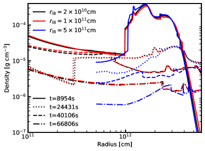
Figure 1: Density (top panel) and velocity (bottom panel) profiles for 1D simulations of model B15 performed with different choices of the radius of the inner grid boundary $r_{\mathrm{IB}}=2\times 10^{10},1\times 10^{11}$ and $5\times 10^{11}\,$cm shown by black, red, and blue lines, respectively. The profiles are plotted at times $t\approx 8950,24430,40100,66800\,$s indicated by different line styles (solid, dotted, dashed, and dash-dotted, respectively). Note that the times plotted are approximate because we output the simulation data at fixed interval numbers of time steps rather than fixed intervals in time. Depending on the choice of the placing of the inner boundary, the inward moving, reverse shock self-reflects at different times. The larger $r_{\mathrm{IB}}$ is, the farther out the self-reflection occurs, and the weaker the self-reflected shocks become. For $r_{\mathrm{IB}}=2\times 10^{10}\,$cm and $r_{\mathrm{IB}}=1\times 10^{10}\,$cm we obtain similar results.

3.2 Beta decay

At early times when the SN ejecta are still optically thick, we expect the $\gamma$-rays produced in the decays of ⁵⁶Ni and ⁵⁶Co to heat up the matter in regions with high concentration of these two radioactive isotopes. This heating should lead to a non-homologous expansion (inflation) of these regions due to $pdV$-work. The total energy available from the decay of ⁵⁶Ni to ⁵⁶Co and the subsequent decay to ⁵⁶Fe is

$$E_{\mathrm{\beta}}\sim(Q_{\mathrm{Ni}}+Q_{\mathrm{Co}})\times\frac{m_{\mathrm{Ni}}}{56m_{u}}=1.9\times 10^{50}\frac{m_{\mathrm{Ni}}}{M_{\odot}}\mathrm{erg}\,,$$ (15)

where $m_{u}$ is the atomic mass unit. For model B15 $m_{\mathrm{Ni}}=0.034M_{\odot}$ and we find $E_{\mathrm{\beta}}^{\mathrm{B15}}=6.5\times 10^{48}\,$ erg. Comparing this with the total kinetic energy at about $1\,$yr, $E_{\mathrm{kin}}^{1\,\mathrm{yr}}=1.4\times 10^{51}\,$erg, we see that $E_{\mathrm{kin}}^{1\,\mathrm{yr}}\gg E_{\mathrm{beta}}$, and, hence, one would not expect a huge change of structures in the ejecta due to the $\beta$ decay. We can test how much of the decay energy is transformed to kinetic energy by comparing results from simulations computed with (B15) and without (B15₀) $\beta$-decay energy input. At $1\,$yr after the explosions we find a difference in the total kinetic energy of the SN ejecta between the two models of $\Delta E^{1\,\mathrm{yr}}_{\mathrm{kin}}\sim 3\times 10^{48}\,$erg, which is approximately half of the total available $\beta$-decay energy $E_{\mathrm{\beta}}^{\mathrm{B15}}$.

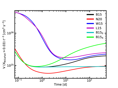
Figure 2: Volume of the structures enclosed by the $3\%$-surface of $X_{\mathrm{NiCoFeX}}$ ($X_{\mathrm{Ni}}+X_{\mathrm{Co}}+X_{\mathrm{Fe}}+X_{\mathrm{X}}>3\%$) rescaled by $t^{-3}$ as a function of time. Homologous expansion would be represented by a horizontal line like for model B15₀ for $t\gtrsim 5\,$h. The expansion in the BSG models B15 and N20 is slower than homologous until $t\lesssim 1\,$d and later it is faster due to the energy input of the $\beta$-radiation causing the inflation of NiCoFe-rich structures. L15 and W15 expand more slowly than homologous until later and their rescaled volumes have their minima around $t\sim 10\,$d. The bubble and finger inflation comes to rest after a few hundred days in all cases.

For freely or homologously expanding ejecta one would expect the volume of any clump or bubble to expand proportional to $r^{3}$ or $t^{3}$. Since the $\beta$ decay provides an additional energy source that may inflate the ⁵⁶Ni-rich structures, we expect deviations from this scaling in our simulations. To quantify this influence of the radioactive decay, we plot the volume enclosed by an isosurface of a constant mass fraction $X_{\mathrm{NiCoFeX}}=0.03$ multiplied by $t^{-3}$ as a function of time in Fig. 2. As expected, the rescaled volume $Vt^{-3}$ of model B15₀ performed without $\beta$-decay expands homologously after about $t\sim 6\,$h, as can be seen by the horizontal cyan line in Fig. 2. For all other models the rescaled volumes of ejecta structures initially containing high Ni mass fractions increase after several hours for the BSG progenitors and after a few days for the RSG progenitors, i.e. the ejecta expand faster than homologous because they inflate. The initial decrease of the rescaled volume is related to the deceleration of the expansion due to the swept up masses in the outer layers still inside the progenitor and the deceleration due to the interaction of the ejecta with the reverse shock formed at the He/H shell interface. As expected, the rescaled volume of model B15_X increases more than that of model B15. The additional energy from the decay of the tracer X leads to the production of more kinetic energy inflating the initially ⁵⁶Ni-rich structures even further. We discuss these differences quantitatively in Section 3.3.5.

After about $150\,$days, the inflation of the ⁵⁶Ni clumps stagnates because the ejecta become optically thin for $\gamma$-ray photons and only a small amount of energy associated with the $e^{+}$, which are released during the $\beta$ decay of ⁵⁶Co, contributes to the heating of the bubbles and clumps. Additionally, a significant fraction of the radioactive material has already decayed after $\tau_{1/2}^{\mathrm{Co}}=77.23\,$d. Similar trends can be observed for all models.

However, since the BSG models B15 and N20 are more compact, the deceleration and interaction with the reverse shock occur and terminate earlier ($t<1\,$d) than for the RSG models ($t\sim 10\,$d). Furthermore, because the liberated energy is deposited within a smaller volume the effect of the bubble and finger inflation sets in also at earlier times, and the inflation is relatively stronger as indicated by faster rises of the rescaled volume in the BSG models. At $t<0.1\,$d the rescaled volume of model W15 (or L15) is more than a factor of $10$ larger than that of B15, and at the end of the simulations around $t\sim 1\,$yr both volumes are almost equal.

3.3 Ejecta structures

3.3.1 Radial velocities

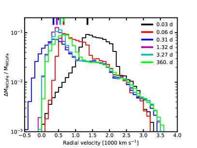
Figure 3: Fractional mass of the ⁵⁶Ni decay chain elements for model B15. The initially rapidly moving ejecta (black line) slow down during the propagation through the progenitor mainly due to the interaction with the reverse shock. After about $t\sim 1\,$d (magenta line) the self-reflected shock and the $\beta$-decay energy input reaccelerate the ejecta until they reach their final velocities at $t\lesssim 1\,$yr (green line). Short lines at the top of the panel indicate the location of the maximum of the corresponding distribution and the bin width of the velocity is $100\,$km/s.

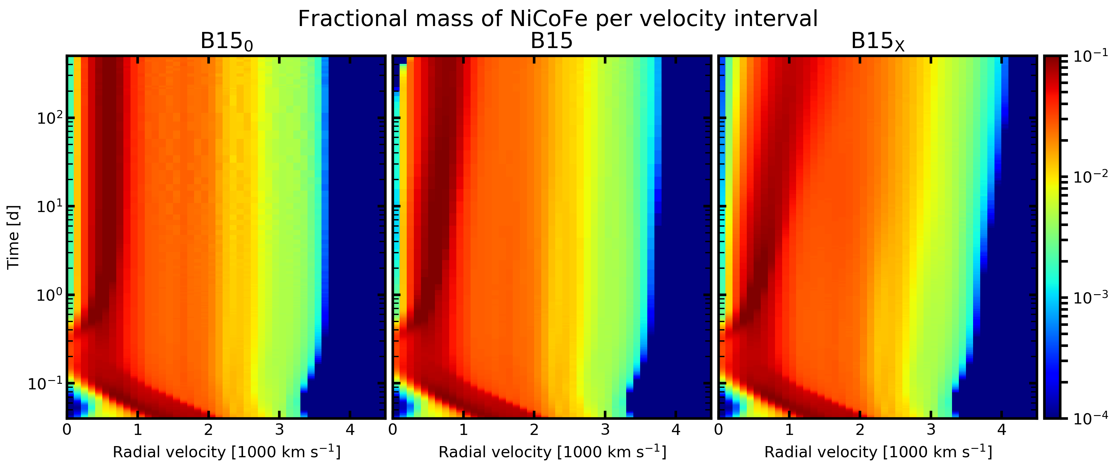
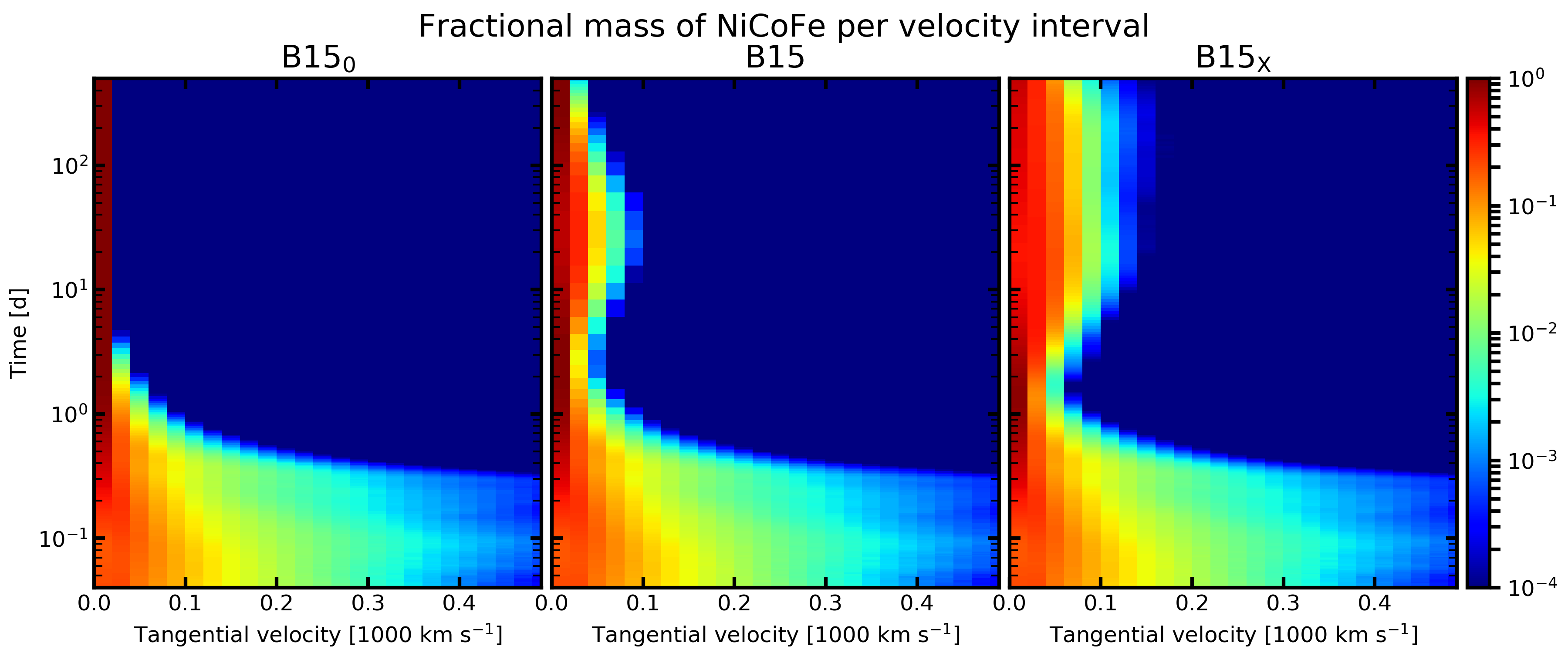
Figure 4: Colour coded is the fractional mass of NiCoFe per velocity bin (x-axis) as a function of time (y-axis) for the first year of the evolution of models computed with the B15 progenitor. Top row: radial velocity. Bottom row: tangential velocity. Different columns show the models without $\beta$ decay (B15₀), with standard $\beta$ decay (B15), and with enhanced $\beta$ decay (B15_X), respectively. After the initial deceleration due to the interaction with the reverse shock up to $t\lesssim 0.5\,$d, the ejecta of models with $\beta$ decay accelerate again until $t\sim 1\,$yr when the expansion becomes homologous. In model B15₀, only the effects of the self-reflected reverse shock can be witnessed.

Both effects discussed in the two preceding sections, namely the $\beta$ decay and the self-reflection of the reverse shock, have a similar impact on the NiCoFe-rich ejecta: they accelerate in particular the innermost slow material. To study their combined action, we investigate the mass distribution of NiCoFe-rich ejecta in the radial velocity space. In Fig. 3, we plot exemplarily the mass fractions per velocity bin of model B15 at different times. At early times ($t<0.5\,$d) the material gets decelerated as can be seen by comparing peaks of the distributions shown with the black, red, and blue curves.

This deceleration is caused by the interaction of the NiCoFe-rich ejecta with the reverse shock formed after the forward shock of the SN crosses the He/H interface (Wongwathanarat et al., 2015). There is even a significant amount of material falling back towards the centre with negative velocities (blue curve at $0.31\,$d). When the reverse shock gets self reflected, it reaccelerates the innermost (and slowest) material such that only a negligible amount of matter has negative velocities at $t=1.32\,$d (magenta curve). Within a few days, the outward-moving, self-reflected shock runs into denser material, and transfers all its energy so that it cannot accelerate the NiCoFe-rich ejecta any longer (cyan curve). At this epoch, the $\beta$ decay of ⁵⁶Ni provides an additional energy source that leads to further acceleration of the NiCoFe-rich ejecta by about $150\,$km/s (see difference in the maxima between the cyan and green curves). The propagation of the fastest moving NiCoFe-rich ejecta can neither be influenced significantly by the self-reflected shock, because it loses its power before reaching them, nor by the $\beta$ decay, because there is not sufficient energy deposition due to the very low mass fraction of ⁵⁶Ni in the fastest ejecta.

In the top panels of Fig. 4, we plot the fractional mass of NiCoFe in given velocity bins in 2D plots as function of time and radial velocity for model B15₀ (left column), B15 (central column), and B15_X (right column). The first few hours proceed nearly identically in all three cases: the reverse shock decelerates the NiCoFe-rich ejecta, causing parts of them to fall back with negative velocities. Then, around $t\sim 0.2\,$d the reverse shock self-reflects and turns outward, accelerating the innermost material to positive velocities. For model B15₀ this acceleration terminates at around 4 days. In contrast, the low-velocity NiCoFe-rich ejecta of models B15 and B15_X continue to accelerate until approximately $150\,$d. Consequently, the mean velocity of the NiCoFe-rich ejecta increases by about $200\,$km/s and even up to $\sim 350\,$km/s for model B15 and B15_X, respectively. In the bottom row of Fig. 4, we plot the fractional mass according to their tangential velocities $v_{t}=\left(v_{\theta}^{2}+v_{\varphi}^{2}\right)^{1/2}$. As for the radial velocity, the tangential velocities of the NiCoFe-rich ejecta, which initially arise mainly due to the growth of RTIs at composition shell interfaces inside the progenitor star (Wongwathanarat et al., 2017), decrease in all models up to about $4\,$d. At later times, $v_{t}$ of the models including $\beta$ decay increases up to a maximum of $100\,$km/s (B15, central panel) and $160\,$km/s (B15_X, right panel). Note that in the latter case much more of the NiCoFe-rich ejecta gets accelerated to $v_{t}>100\,$km/s and the tangential velocities need longer time to decline to very low values. The maximal velocities in model B15 are reached after $20\,$d and then $v_{t}$ decreases until it becomes negligible again at around $1\,$yr. At this point the SN ejecta have attained homology for this model, and we do not expect further strong effects of the $\beta$ decay of ⁵⁶Ni and ⁵⁶Co on the structure of the NiCoFe-rich ejecta. In model B15_X, even after more than $1\,$yr the tangential velocity is still significant.

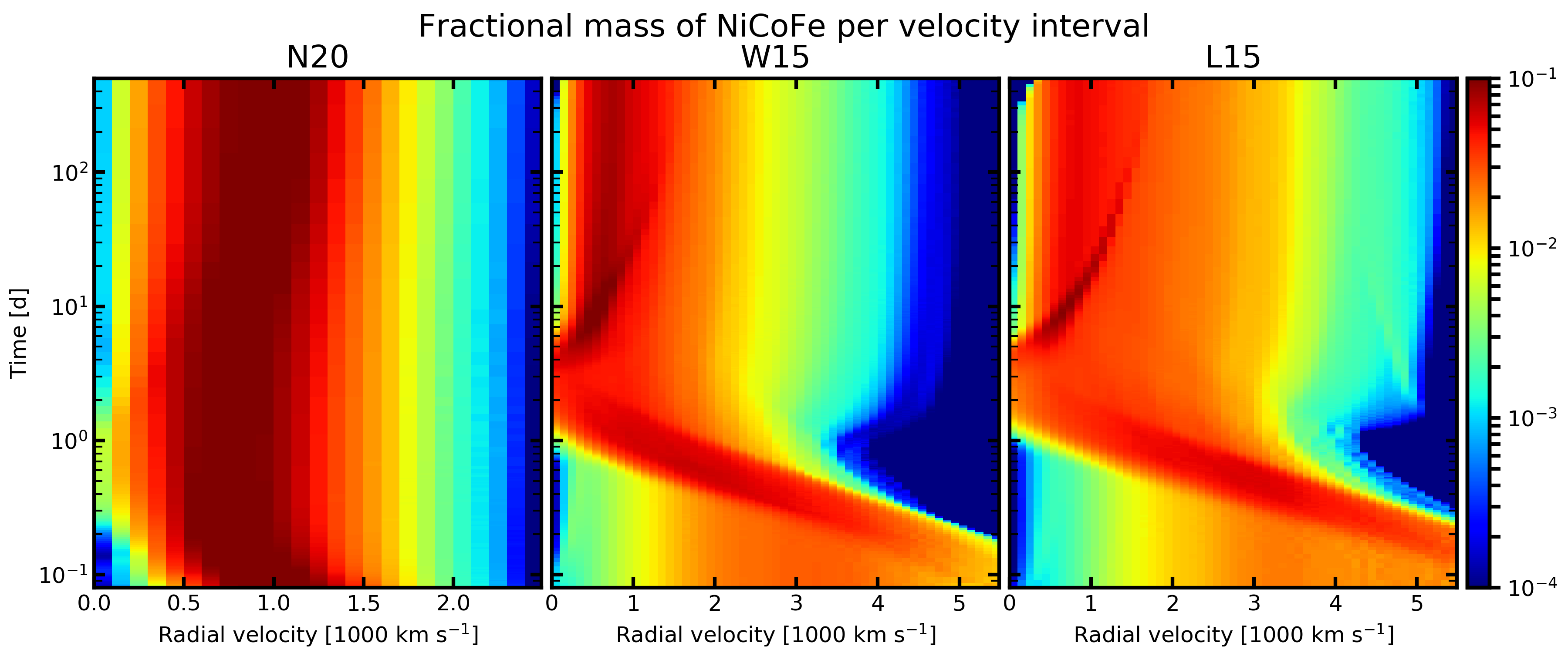
Figure 5: Same as top row of Fig. 4 but for models N20, W15, and L15. Model N20 has the weakest reverse shock and, hence, the weakest acceleration due to the self-reflected shock. The two RSGs have higher initial velocities (because of more efficient radial mixing of heavy elements) and the reverse shock reaches the central (slow) part of the ejecta at later times ($t\sim 5\,$d). For all models the acceleration stalls after a few hundred days. Note the different scale of the $x$-axis for model N20.

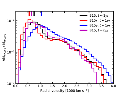
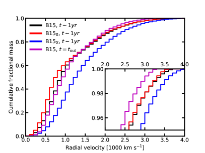
Figure 6: Fractional mass (top panel) and cumulative fractional mass (bottom panel) of NiCoFe in radial velocity bins of $100\,$km width at shock breakout (magenta) and after $t\sim 1\,$yr of the evolution of the models B15, B15₀, and B15_x, respectively. At shock breakout all models have an almost identical velocity distribution and we only show that of model B15. Short lines at the top of the panel indicate the location of the maximum of the corresponding distribution. The inset in the lower panel shows the distributions of the fastest 5% of the NiCoFe material.

Figure 7: Fractional mass (top panel) and cumulative fractional mass (bottom panel) of NiCoFe in radial velocity bins of $100\,$km width at shock breakout and after $t\sim 1\,$yr of the evolution of the models N20, W15, and L15, respectively. Short lines at the top of the panel indicate the location of the maximum of the corresponding distribution. The inset in the lower panel shows the distributions of the fastest 5% of the NiCoFe material.

The time evolutions of the NiCoFe mass distributions in the radial velocity space of the other three models, N20, W15, and L15, are given in Fig. 5. In model N20, the deceleration of the NiCoFe-rich material is not as strong as in the other two models, i.e. there is almost no NiCoFe-rich material with negative radial velocities. However, since the reverse shock is very weak in this model, the self-reflected shock is also very weak. Acceleration of NiCoFe-rich ejecta after $t\sim 1\,$d is almost entirely due to the $\beta$-decay energy deposition. The two RSG models, W15 and L15, have a strong reverse shock that decelerates the NiCoFe-rich ejecta drastically. Consequently, after a few days there is some NiCoFe-rich material with negative velocities in these two models. As for model B15, the reverse shock then self-reflects and accelerates the innermost ejecta outward. Around the same time, a significant amount of the radioactive ⁵⁶Ni has decayed, and the deposited $\beta$-decay energy heats up the ejecta and contributes to the reacceleration of NiCoFe-rich material. Around $t\sim 1\,$yr, the acceleration stagnates and homologous expansion follows. The reverse shock in the BSGs is generally weaker than in the RSGs, because the density drop at the He/H-interface is less steep in the BSGs (Wongwathanarat et al., 2015). The shallower density gradient leads to slower acceleration of the shock when crossing this interface and, consequently, the following deceleration inside the H-shell is less drastic. Therefore, the reverse shock, forming as a consequence of this deceleration, is weaker in models N20 and B15.

Next we will study how the mass distribution of the NiCoFe-rich ejecta changes from the shock breakout to $t\sim 1\,$yr after the onset of the explosions. The graphs for models B15, B15₀, and B15_X are given in Fig. 6. Without $\beta$ decay, the peak of the mass distribution shifts to lower values of the radial velocity (compare magenta and red curves in Fig. 6). In contrast, the peaks of the distributions shift towards higher velocities at late times for models computed with $\beta$ decay. The highest velocities of the NiCoFe-rich ejecta are larger at late times in all cases, regardless of whether the $\beta$ decay is included or not. Even without $\beta$ decay, the ejecta still did not expand homologously at shock break out for model B15 (see also Fig. 4).

In Fig. 7, we show the fractional mass distribution versus radial velocity for models N20, W15, and L15. In all cases, the maxima of the distributions at $t\sim 1\,$yr are at lower velocities than during the shock breakout. At the breakout time, the bulk of the NiCoFe-rich matter is still decelerating due to the interaction with the reverse shock. In contrast to model B15, the acceleration due to the self-reflected reverse shock and the $\beta$ decay is not sufficient to reach bulk velocities larger than during the shock breakout. However, similar to model B15, there is sufficient acceleration of the high-velocity tail of the mass distributions for models W15 and L15 that the tails extend to higher velocities at late times $t\sim 1\,$yr, even though the bulk of the matter is moving slower than before. This acceleration of the high-velocity component happens still at early times until about several days (see Fig. 5) and the effects of the $\beta$ decay are subdominant. The fractional mass distribution of model N20 has different characteristics. The fastest moving NiCoFe-rich ejecta of this model are almost at the same velocities at $t=t_{\mathrm{out}}$ and $t\sim 1\,$yr, i.e. the fastest material was expanding homologously almost since it left the progenitor star, and the $\beta$-decay energy input was not able to accelerate this material significantly.

We can study this behaviour also by looking at the mean velocities of the NiCoFe-rich ejecta at $t\sim[t_{\mathrm{out}},1\,$d$,10\,$d$,1\,$yr$]$ in Table 3. During and shortly after the breakout, all models have a strong decrease of the mean velocity. Note that for model L15 $t_{\mathrm{out}}\sim 1.1\,$d, such that also in this model the mean velocity decreases after the breakout time. After this period, the models show different behaviours. The B15₀ model without $\beta$ decay has only a very mild acceleration of the mean velocity between $t=1\,$d and $t=10\,$d and remains constant afterward, indicating that it reaches homologous expansion after a few days. In model B15 with standard $\beta$ decay, there is significantly more acceleration even after $t=10\,$d, and model B15_X has the strongest velocity increase of up to $30\%$.

From $t=1\,$d until the end of our simulations, the mean velocities in model B15 and B15_X increase by about $100\,$km/s and $400\,$km/s, respectively. This shows that the $\beta$ decay has a significant imprint on the final velocities and, thus, has to be considered in the simulations. The other three models show similar trends as model B15 or B15_X. Around the time of the shock breakout, the mean velocity of the NiCoFe-rich ejecta decreases, while at latest after a few days, an acceleration occurs. In contrast to model B15 or B15_X, the mean velocities of all other models during shock break out are not reached again until the end of the acceleration phase. In addition to the mean velocity, we give the velocity of the fastest one percent of the NiCoFe-rich ejecta in Table 3. Most of the acceleration is finished after ten days and only the velocity of model B15_X increases significantly by $200$ km/s until one year. Comparing the different models, L15 has the fastest moving NiCoFeX-rich ejecta. The higher velocities are a direct consequence of the high explosion energy of that model, see Table 1.

time	B150	B15	B15X	N20	W15	L15
$t_{\mathrm{out}}$	1.22	1.22	1.22	1.18	1.40	1.79
$1\,$d	1.12	1.12	1.17	0.89	1.39	1.90
$10\,$d	1.14	1.16	1.33	0.93	1.15	1.60
$1\,$yr	1.14	1.22	1.52	1.00	1.29	1.73

Table 2: Mean velocities of NiCoFe at different times in $1000$ km/s. Note that $t_{\mathrm{out}}$ for Model L15 is $t_{\mathrm{out}}\sim 1.1\,$d, while all other times of the breakout are shorter than one day (see Table 1).

time	B150	B15	B15X	N20	W15	L15
$t_{\mathrm{out}}$	3.19	3.18	3.19	2.08	3.31	3.92
$1\,$d	3.46	3.45	3.47	2.05	3.32	3.92
$10\,$d	3.48	3.48	3.60	2.06	4.09	4.81
$1\,$yr	3.48	3.54	3.80	2.08	4.16	4.89

Table 3: Mean velocities for the fastest one percent of the NiCoFe-rich ejecta in $1000\,$km/s.

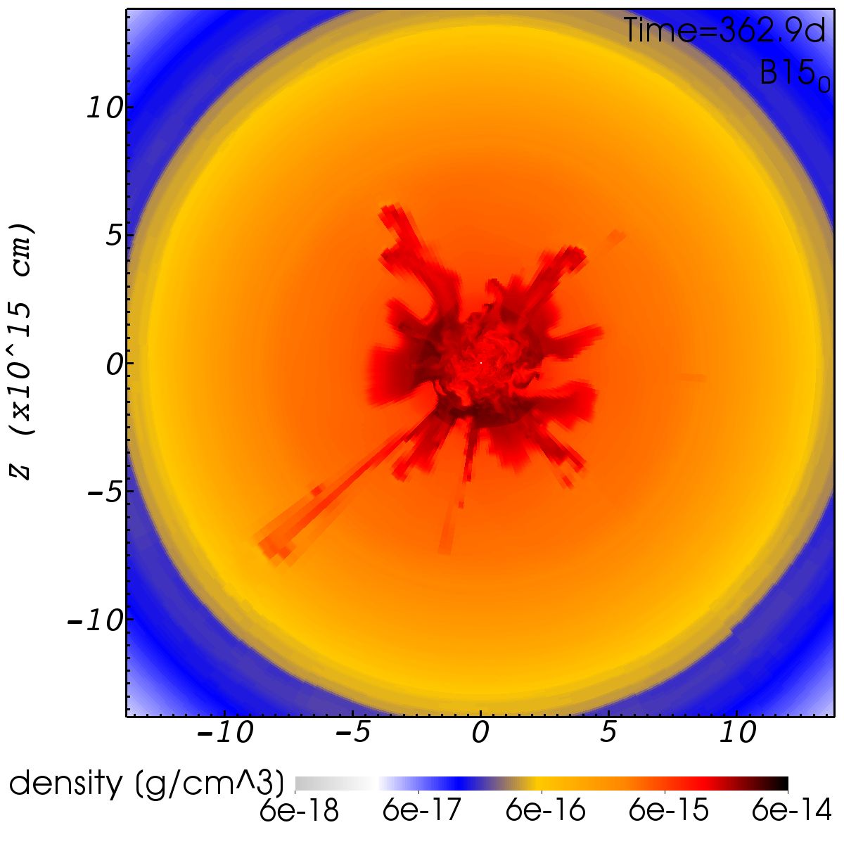
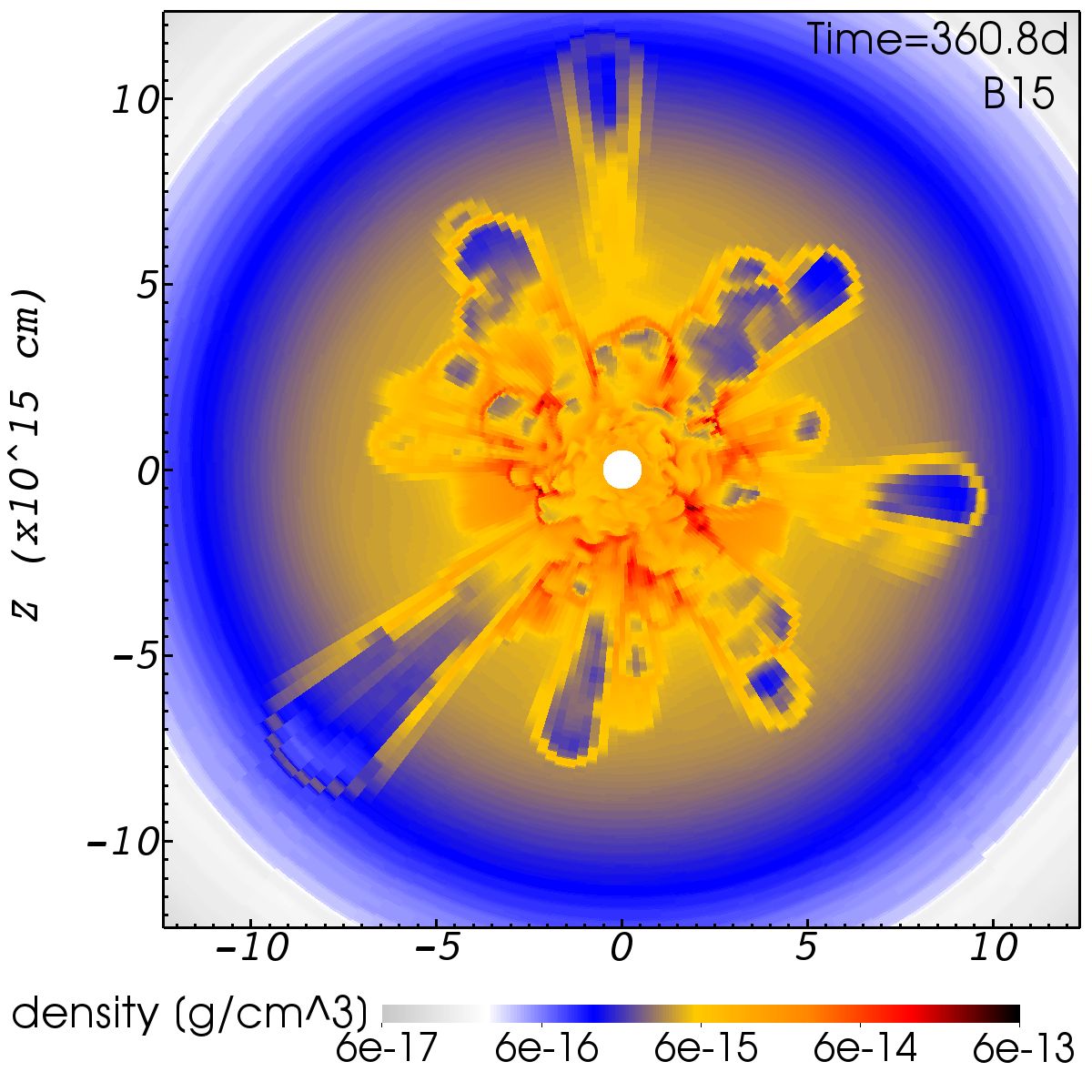
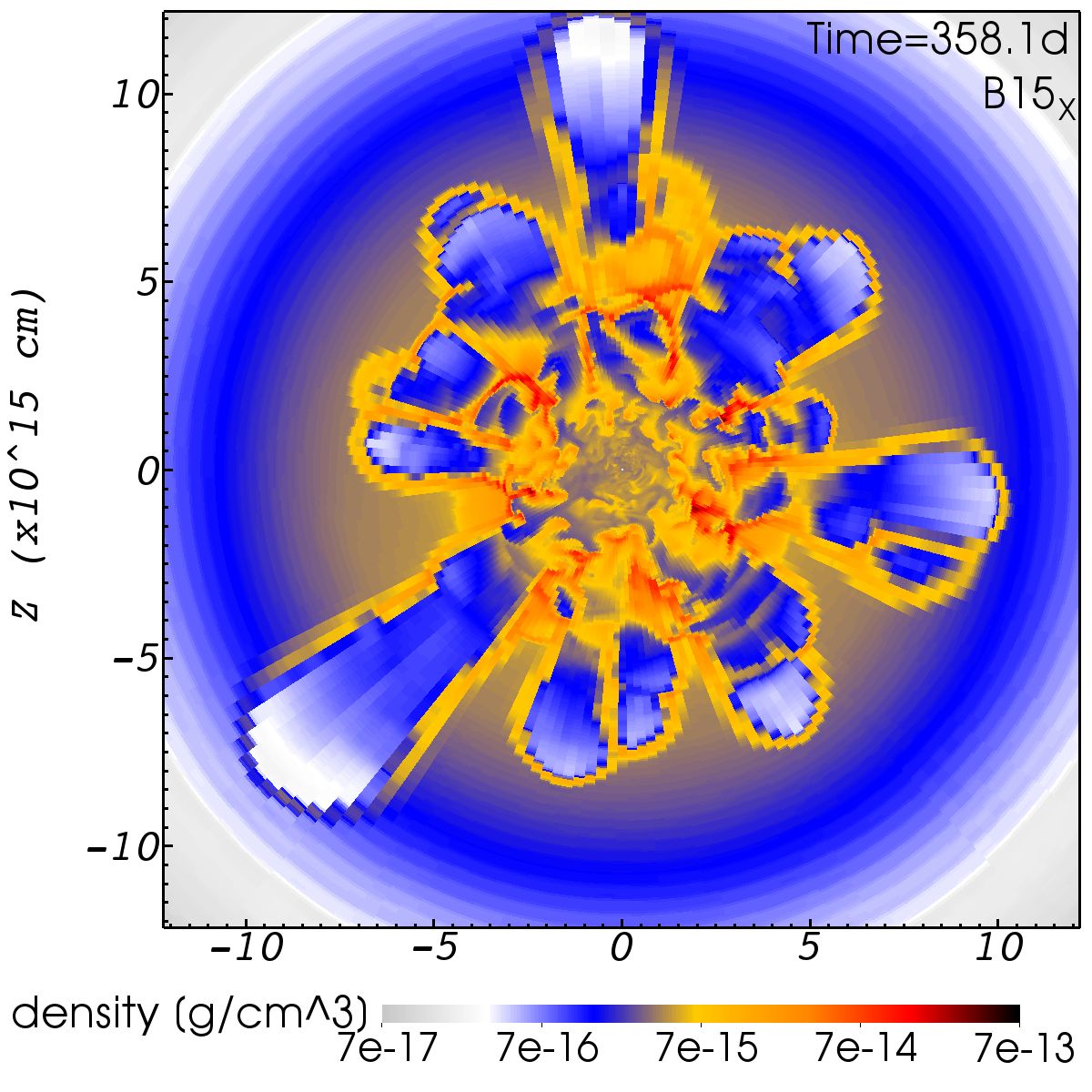
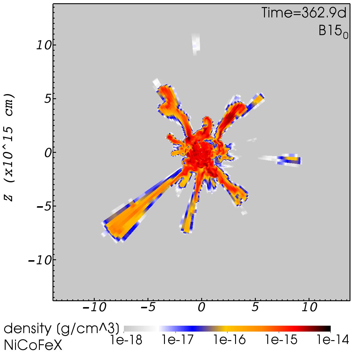
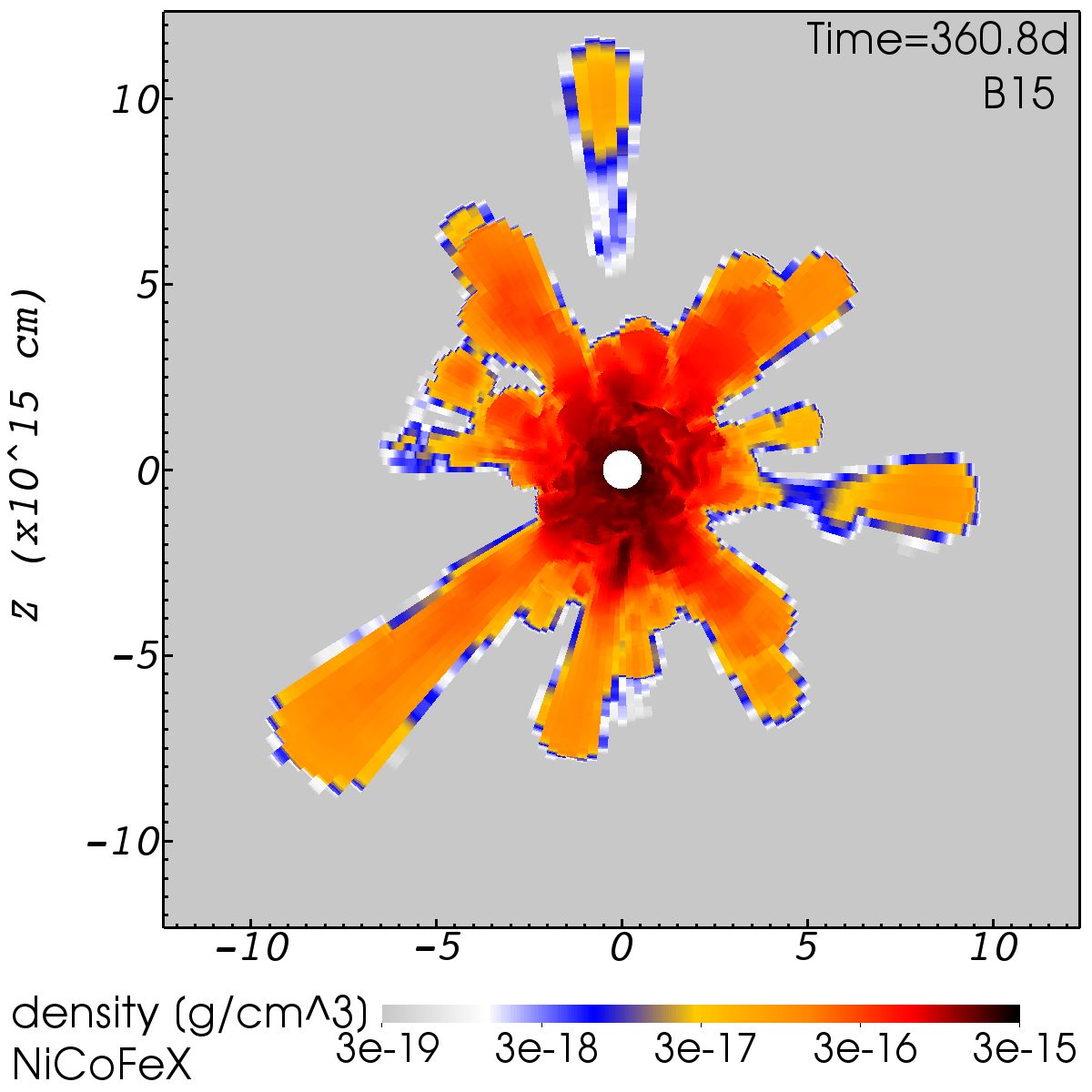
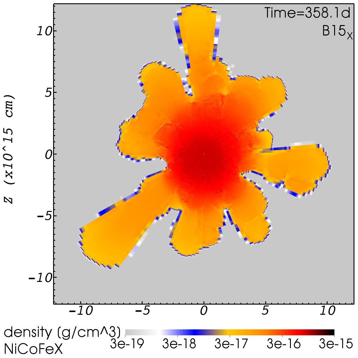
Figure 8: Top row: Density slices of models B15₀ (left panel), B15 (central panel), B15_X (right panel) in the x-z-plane around $t\sim 1\,$yr. Bottom row: Slices of the density of NiCoFeX of the corresponding models in the same plane and at the same time. The density scale is logarithmic in all panels. Without $\beta$-decay (B15₀) the NiCoFeX-rich RT fingers stay unchanged and are over dense relative to their surroundings. When including $\beta$ decay (B15) in the simulation, the fingers inflate and become underdense. Due to the larger amount of radioactive material, Model B15_X has a larger inflation of the fingers and the NiCoFeX distribution inside the fingers becomes also more uniform. For efficiency reasons, as discussed in Section 2.1, we cut out the central white region during the simulation. This is visible in particular for model B15 (see also Footnote 1 in Section 2.1).

3.3.2 Density distributions

Here, we investigate the effect of the energy input due to the $\beta$ decay on the ejecta structures by plotting slices of the total density $\rho^{\mathrm{tot}}$ and the density of NiCoFeX $\rho_{\mathrm{NiCoFeX}}$. The corresponding plots at $t=1\,$yr for models B15₀, B15, and B15_X are shown in Fig. 8. In the top left panel for model B15₀, there are pronounced elongated ejecta structures, in particular in the negative $z$ and negative $x$ direction. These structures originate from the growth of RTI during the propagation of the SN shock through the progenitor envelope. Note that only in model B15₀ the density decreases from the centre of these structures towards the exterior, i.e. these RT fingers have higher densities than the ambient matter. In the bottom left panel, one can see that these overdense RT fingers are very rich in NiCoFeX. In the model without $\beta$ decay these structures are completely developed already at around $t\sim 1\,$d, and do not change morphologically afterwards, i.e. in model B15₀ the Ni-rich ejecta are already expanding homologously after $t\sim 1\,$d. In contrast, the models including $\beta$ decay have Ni-rich fingers that have lower densities than the matter around them (central and right top panels). The decay of radioactive material increases the internal energy. This energy increase heats up the NiCoFeX-rich ejecta, and they start to expand by doing $pdV$ work against their surroundings. Consequently, the densities inside the NiCoFeX-rich clumps decrease (compare bottom left to right panels for decreasing densities with increasing $\beta$ decay). This inflation of ejecta inside Ni-rich fingers sweeps up ambient matter and compresses this material to higher densities. As a result, regions of density enhancements build up at the border between decaying and non-decaying ejecta. In model B15_X, where the $\beta$-decay energy input is highest (top right panel), the fingers or bubbles inflate more than in model B15, and the density contrasts between the interior and the walls of the finger borders are also more pronounced (compare the bubble borders of the elongated finger in the negative z- and x-directions). Regions rich in NiCoFeX expand more than NiCoFeX-poor regions. Therefore, the density of NiCoFeX smears out and becomes more uniform within the finger and the central bubble. Compare central and right bottom panels, where the density variations inside the NiCoFeX-rich regions decrease significantly.

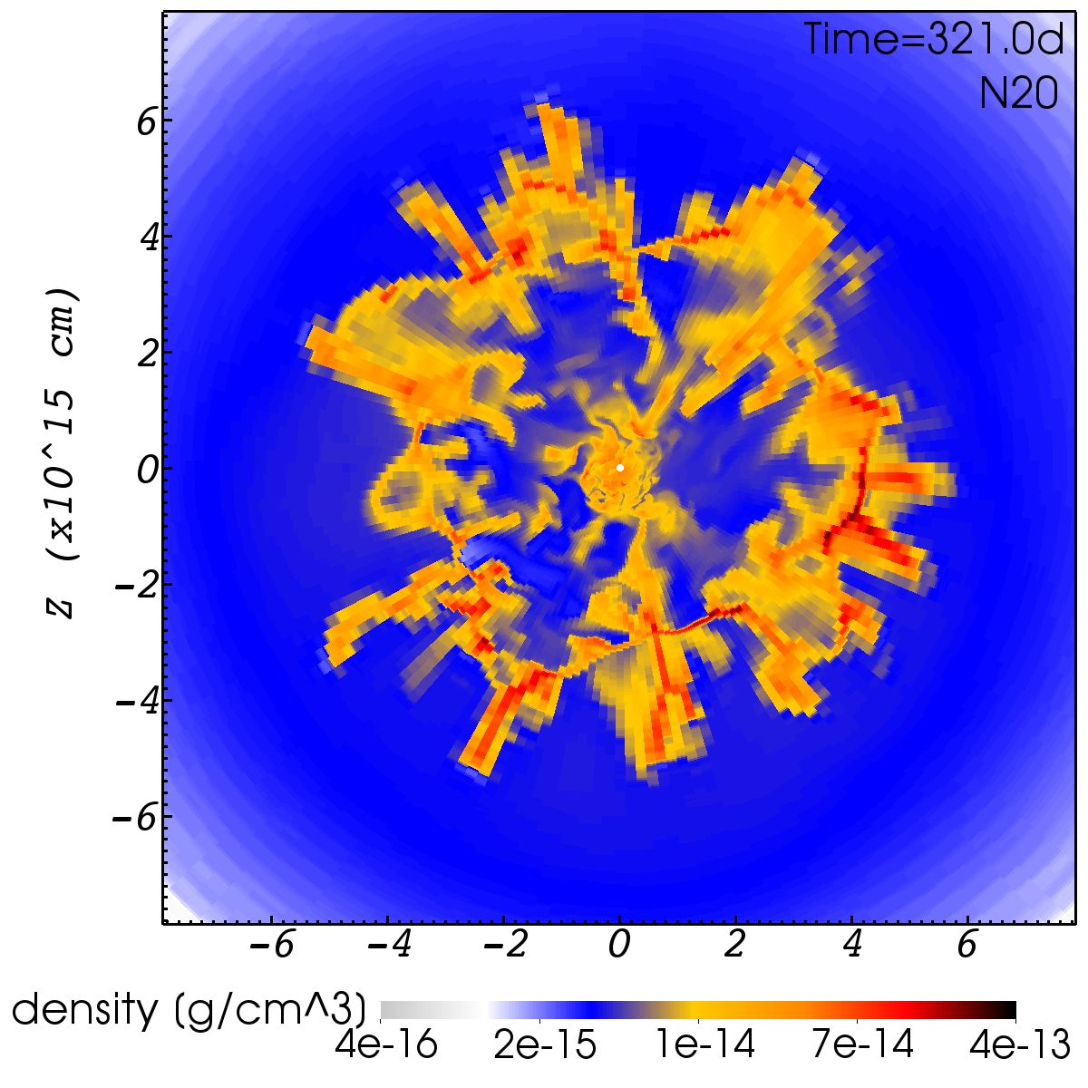
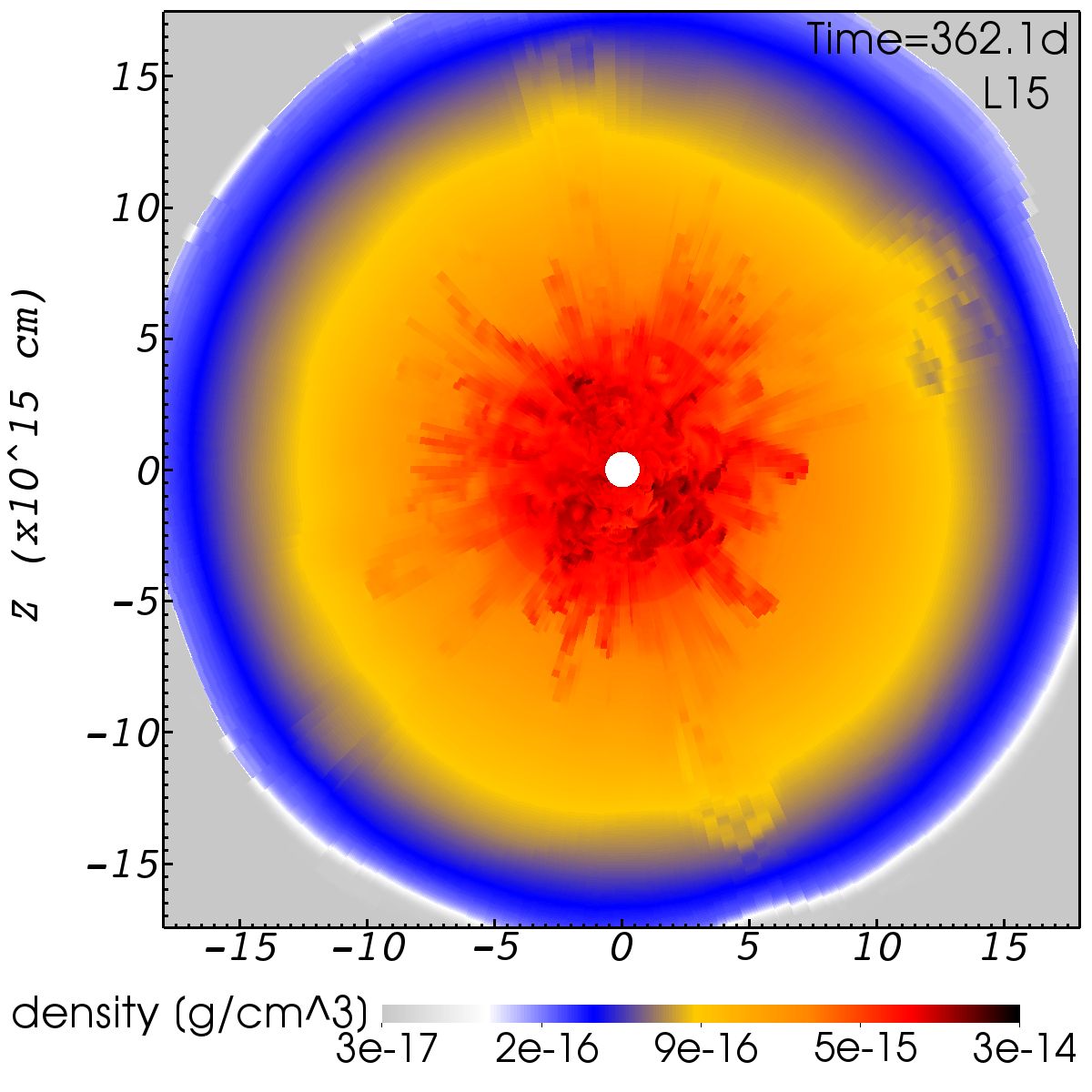
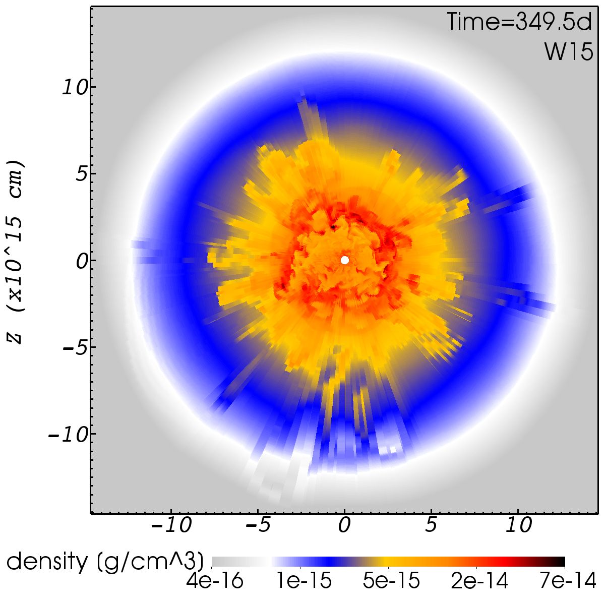
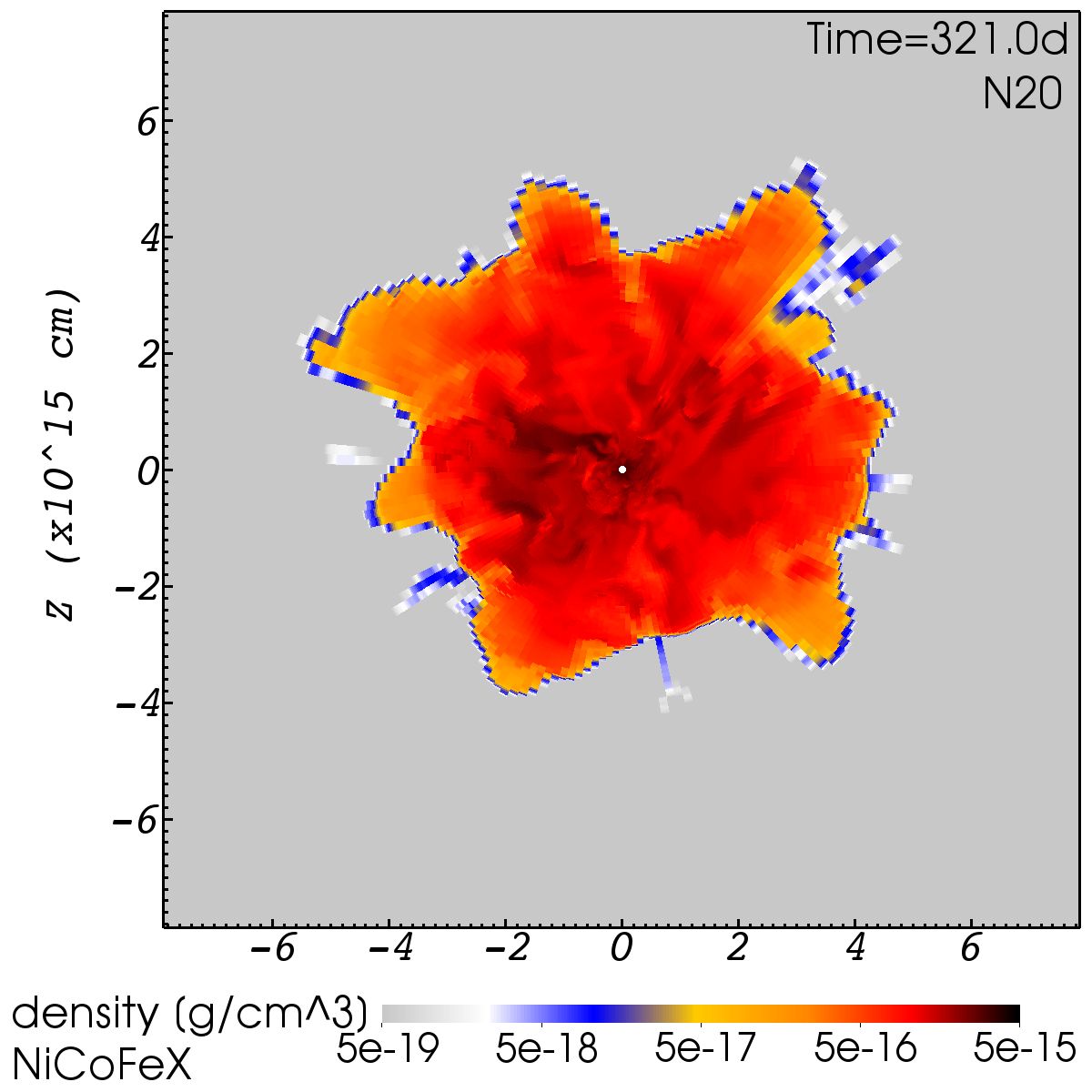
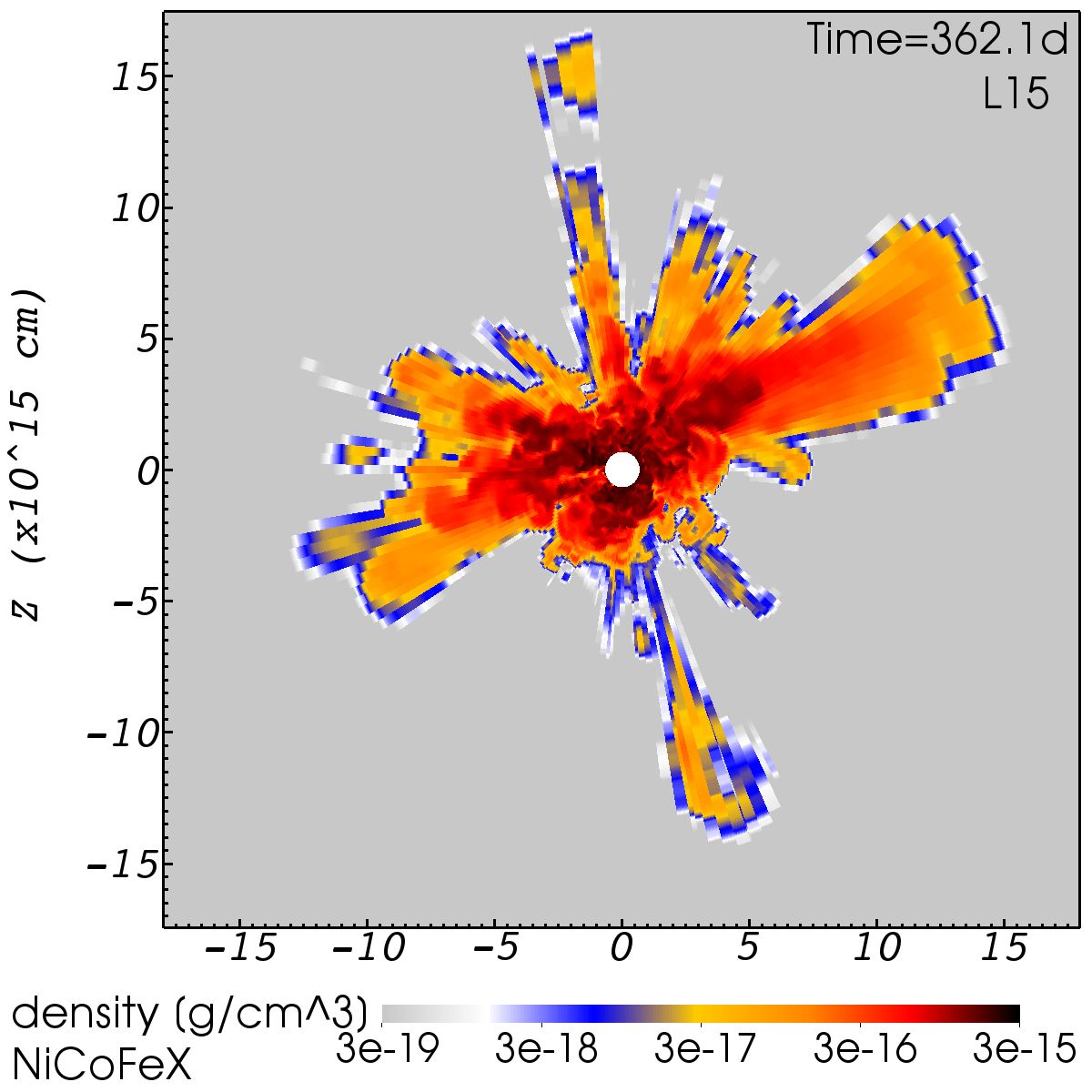
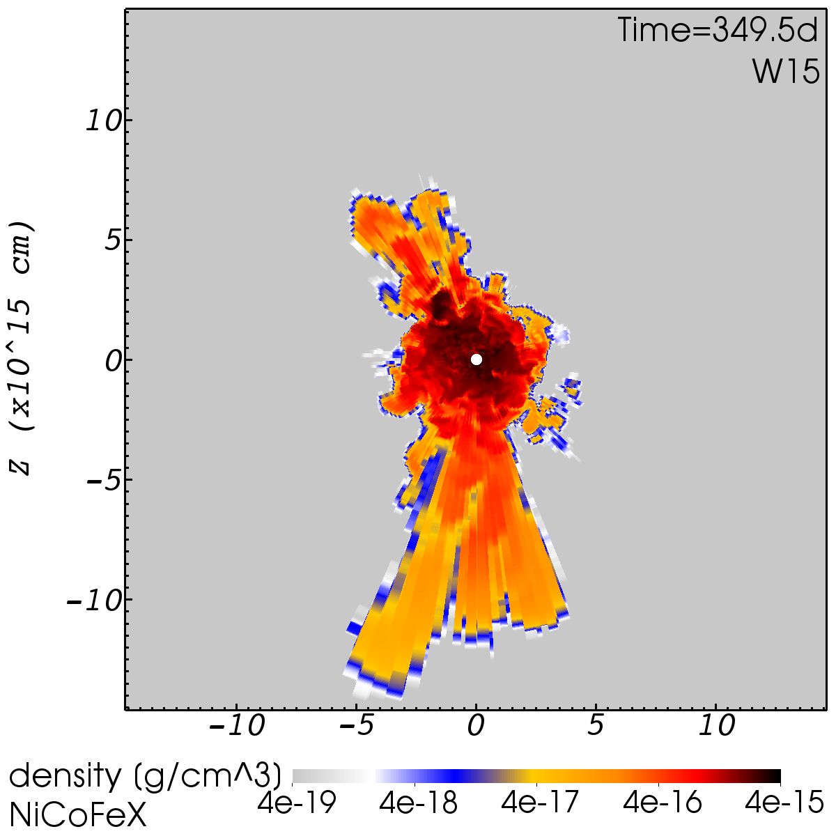
Figure 9: Top row: Density slices of models N20 (left), L15 (centre), W15 (right) in selected planes containing the most pronounced RT fingers at $t\sim 1\,$yr. Bottom row: Slices of the density of NiCoFeX of the models in the same planes and at the same time. The density colour scale is logarithmic in all cases. In models W15 (top right) and L15 (central top panel) underdense regions can be seen inside of inflated RT fingers (compare to the similar to results for model B15 in Fig. 8), where the corresponding plots of the NiCoFeX densities (bottom right and central panel, respectively) display an extended finger. However, in the RSG models, the density contrast of these RT fingers compared to their surroundings is less pronounced than in model B15. The NiCoFeX-rich ejecta in model N20 are organized in a shell-like structure with very short RT fingers that do not inflate significantly. During the simulation, we cut out the central white region.

Slices of the density distribution of models N20, W15, and L15 are given in Fig. 9. Model W15 (top right panel) is the most similar model compared to B15. However, the effect of the inflation of the NiCoFeX-rich fingers is not as apparent as in B15. See also Fig. 2, where the rescaled NiCoFeX-rich volumes for model B15 roughly double from their minima until the end of the simulation, while the corresponding volumes for models W15 and L15 increase by at most $50\%$. The absolute volume of the NiCoFeX-rich matter is similar in all three models. For model W15, there are three grouped RT fingers in negative z-direction (bottom right panel in Fig. 9) that have higher density (orange) in the borders between them compared to their interiors. In general, the interior volumes are underdense (white) compared to the mean density (blue) at the same radius (top right panel). As for model B15 and B15_X, there is a NiCoFeX-rich bubble in the centre, which has lower densities than the surroundings, and the walls of this bubble are significantly overdense. The main reason for the weaker relative inflation of the RT fingers is that this model is already more extended at early times ($t\sim 1\,$d) when the $\beta$ decay starts to become significant and that the initial structures occupy much larger volumes compared to model B15. The region where the $\beta$-decay energy is deposited is much less compact and, hence, the internal energy increase does not lead to a large growth of the structures in the two RSGs. At $t\sim 1\,$yr, the sizes of the NiCoFeX-rich structures are similar to those in B15, because the fingers and the bubble of model B15 have inflated more (see also Fig. 2).

The density distribution of model L15 (central panels of Fig. 9) is very similar to model W15. As in the other models, NiCoFeX-rich regions have slightly lower local densities compared to their surroundings as can be seen in particular for the NiCoFeX-fingers in all directions, top, bottom, left and right in the bottom central panel. However, in model L15, the contrast in $\rho^{\mathrm{tot}}$ between the inner NiCoFeX-rich bubble or the fingers on one side and the corresponding borders on the other side is less pronounced than in W15, and much less than in B15. The RT fingers in model L15 are almost invisible in the top, central panel of Fig. 9, and are hardly visible as the white bubbles in the blue shell in model W15 in the top, right panel of the same figure. However, the fingers are clearly visible in model B15 in the top central panel of Fig. 8. The weaker density contrast between the finger boundaries and their interiors in the RSGs is related to the significantly lower density in the H-envelope of the RSGs compared to that in the BSGs (see figures 1 and 2 in Wongwathanarat et al., 2015). Therefore, the entropy and pressure in the envelopes of the BSGs after the passage of the forward shock is lower than those in the RSGs. This lower ambient pressure facilitates the expansion of the NiCoFeX-rich fingers in the case of model B15. In addition, the expansion into the denser H-envelope of the BSG sweeps up more mass than in the more dilute H-envelopes of the RSGs. Consequently, the stronger expansion into a denser environment leads to stronger density contrasts for model B15 compared to the RSGs.

Model N20 is very different from all other models. First, the reverse shock from the He/H-interface and its self-reflected shock are weaker than in the other models (see left panel in Fig. 5). Therefore, the central ejecta are almost not decelerated by this reverse shock. In addition, they are only mildly reaccelerated almost exclusively by the energy input due to $\beta$ decay. This leads to a thin dense, corrugated shell of swept-up material with a radius of $r\sim 4\times 10^{15}\,$cm as shown in the top left panel of Fig. 9. This shell is strongly fragmented into many RT fingers, which are significantly smaller than the extended fingers of the other models. Comparing the top and the bottom left panel of Fig. 9, we see that most of the NiCoFeX is enclosed by the dense, corrugated shell. Since the shell is not as much affected by the RTIs as the other models (see Wongwathanarat et al., 2015, for a detailed discussion), there is no significant mixing of ⁵⁶Ni into the small fingers and the latter do not contain sufficient ⁵⁶Ni to power significant inflation by radioactive decay. Most of the $\beta$-decay energy is released in the central bubble, leading to a more spherical expansion compared to the other models.

3.3.3 Inflation of NiCoFe-rich fingers

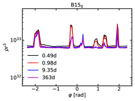
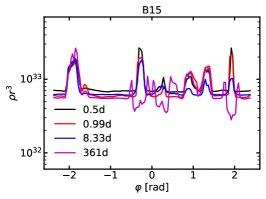
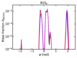
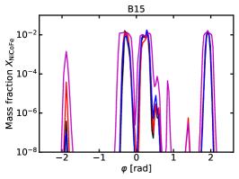
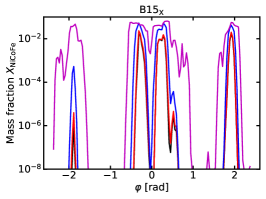
Figure 10: Top row: Density rescaled by the time-evolving $r^{3}$ of initially overdense fingers in models B15₀, B15, and B15_X at different times as indicated in the legend. Without $\beta$ decay, the density enhancements stay approximately at the same angular positions with the same angular extent (left panel), while the $\beta$ decay leads to an inflation of the initially overdense regions, which become underdense (central panel). If there is more radioactive material (top right panel, B15_X), the densities in the underdense regions decrease further. At the borders of these regions material gets compressed into thin ‘walls’. Bottom row: Mass fractions $X_{\mathrm{NiCoFe}}$. The overdense regions (compare with top row) that initially contain significant amounts of ⁵⁶Ni inflate, while overdense regions initially poor in ⁵⁶Ni do not change significantly.

As discussed in Section 2.2, $Vr^{-3}$ or $Vt^{-3}$ should be a constant for homologously expanding ejecta. Equivalently, this holds for $\rho r^{3}$. Therefore, we plot the density rescaled by $r^{3}$ as a function of $\varphi$ at given $r$ and $\theta$ for different times and for the three models B15₀, B15, and B15_X in the top row of panels in Fig. 10. At the beginning of the simulation at $t=0.0365\,$d, we choose $r=9.7\times 10^{11}\,$cm and $\theta=0.578\pi$, which is outside of the central bubble. We follow the evolution of this location in the flow by integrating the radius in time with the local fluid velocity. We chose this initial location because here we see a few of the fastest ⁵⁶Ni fingers as local density enhancements like at $\varphi\sim[-2.0,-0.2,0.2,2.0]$ for $t\sim 0.5\,$d. These density enhancements are related to the NiCoFe-rich fingers. In the bottom panels of the figure, we show the corresponding mass fractions of ⁵⁶Ni and its decay products. High densities usually appear where $X_{\mathrm{NiCoFe}}\gtrsim 5\times 10^{-3}$. There are some exceptions around $\varphi\sim-2$, $\varphi\sim 0.9$, and $\varphi\sim 1.1$ where the displayed part of the fingers is not ⁵⁶Ni enriched initially. In these cases, ⁵⁶Ni is located further inside the respective finger. The evolution of the model without $\beta$ decay is almost homologous from the beginning, i.e. $\rho r^{3}$ is constant and existing structures do not change during the evolution (see top and bottom left panels in Fig. 10). Differences between different time steps mainly arise due to the inaccurate time integration of the reference radius. The corresponding integration was done as a post processing and, thus, the time stepping was limited to the output times of the 3D simulation. In contrast, the models including $\beta$ decay show a significant change of their structures. For model B15 (central panels in Fig. 10), the initial high densities at $t=0.5\,$d (black curve) at $\varphi\sim-0.2$, $\varphi\sim 0.2$, and $\varphi\sim 2.0$ decrease slowly until day $10$ (red and blue curves) and even turn into underdense regions at $t\sim 1\,$yr. All this occurs at the highest mass fraction $X_{\mathrm{NiCoFe}}$ (compare bottom central panel of Fig. 10). The energy input in form of decay energy is used to do $pdV$ work on the exterior of the initially ⁵⁶Ni-rich fingers which inflate. Consequently, the density inside the fingers decreases with respect to the surroundings, and the inter-finger, ⁵⁶Ni-poor regions get compressed into thin filaments with high densities, which we call finger walls or borders. During this compression NiCoFe gets also mixed in the border region. Other initial overdense regions without significant amounts of ⁵⁶Ni ($\varphi\sim[-2.0,0.9,1.1]$) do not change significantly. However, the mass fraction of ⁵⁶Ni at $\varphi\sim-2.0$ increases for this model with time. This is material, which is accelerated (also radially) due to the $\beta$ decay, and, thus, penetrates the previously ⁵⁶Ni poor, overdense region. All the described effects are even more pronounced in model B15_X (right panels). Here, the maximum density contrast with respect to the mean density $\rho r^{3}\sim 6\times 10^{32}\,$g at $t\sim 1\,$yr is a factor $~{}10$ in the overdense regions and $1/3$ in the underdense regions, resulting in density enhancements of up to more than one order of magnitude between the interior and the wall.

3.3.4 3D structures of NiCoFeX-rich fingers

In this section we investigate the 3D structures for all of our models and how they change with time. Following Wongwathanarat et al. (2015), we use the iron-group elements around $A=56$ like ⁵⁶Ni, ⁵⁶Co, ⁵⁶Fe and X (NiCoFeX) to determine the surface of the structures that characterize metal mixing from the SN centre into the outer shells of the star. To define the isosurfaces, we sum up the mass of all cells with the highest mass fractions $X_{\mathrm{NiCoFeX}}$ until we reach a certain percentage of the total mass of NiCoFeX. The mass fraction that encloses all this mass defines our isosurface. The corresponding mass fractions are indicated in each plot. For example in Fig. 11, the isosurfaces containing $90\%$ of the mass of NiCoFeX in cells that have the highest mass fractions are plotted. The remaining $10\%$ of the NiCoFeX is contained in ejecta with lower NiCoFeX mass fractions. Note that the magnitude of $X_{\mathrm{NiCoFeX}}$ defining the isosurfaces decreases with time. Due to the expansion and the related mixing of the matter, $X_{\mathrm{NiCoFeX}}$ decreases in particular in the outermost layers of the fingers.

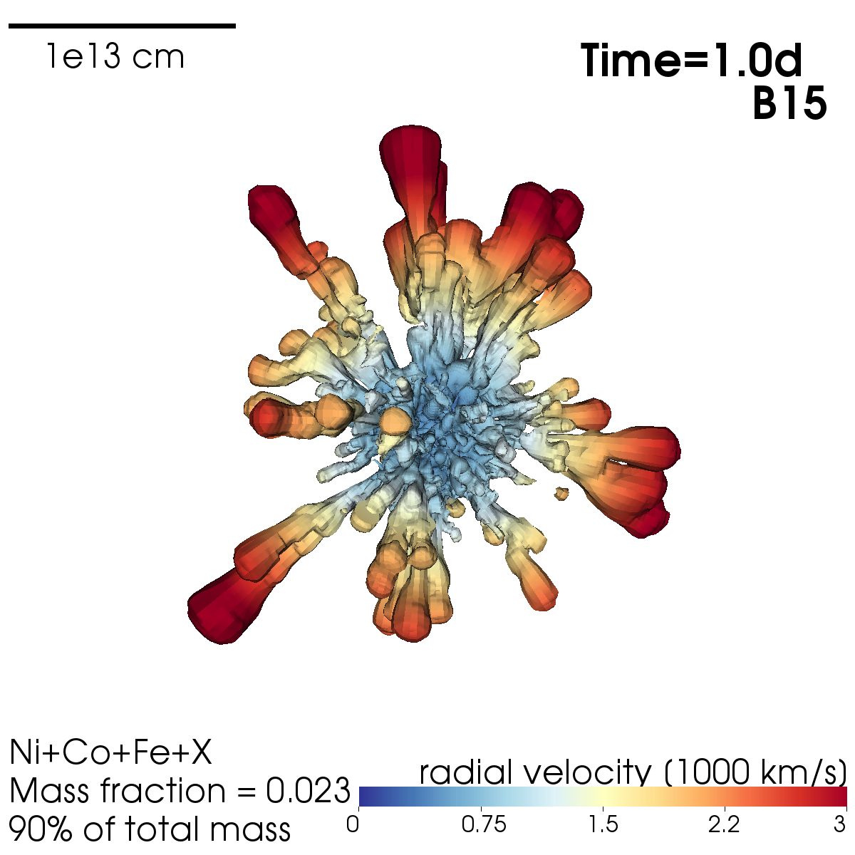
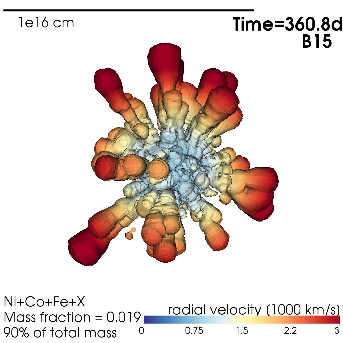
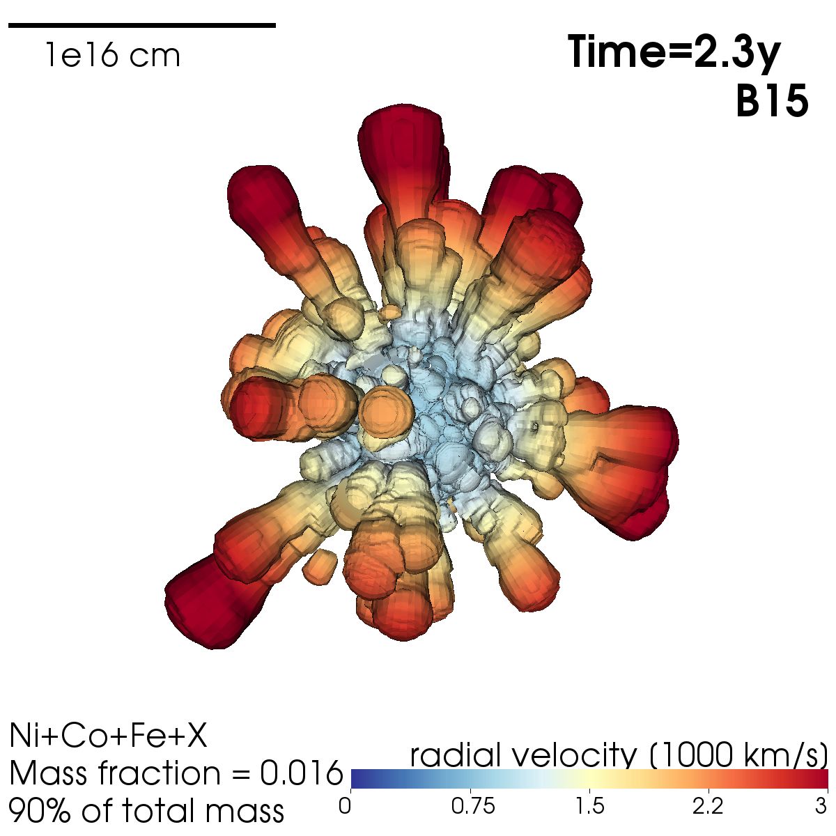
Figure 11: Isosurface plots of constant mass fraction containing $90\%$ of the mass of NiCoFeX for different times of model B15. After the reverse shock (spherical shell in the top, left panel, $t\sim 0.9\,$h) retreats to the centre and the initial RTIs grow until $t\sim 1\,$d (top, right panel), the fingers start to inflate due to $\beta$-decay energy input (bottom, left panel, $t\sim 1\,$yr). After $t\lesssim 1\,$yr the inflation stalls and the structures do not change significantly. The NiCoFeX mass fractions defining the isosurfaces are indicated in each panel.

The top panel of Fig. 11 shows NiCoFeX-rich structures before shock breakout. The reverse shock is visible as the spherical shell which is penetrated by some faster NiCoFeX-rich fingers. The reverse shock slows down the central ejecta compared to the extended RT fingers and leads to an apparent contraction of the central part compared to homologous expansion. Note that the scale of the plots at different snapshots increases linearly with time and, thus, follows homologous expansion. The fingers become more prominent at $t\sim 1\,$d (second panel). Then the $\beta$-decay energy input becomes significant and the thin, elongated NiCoFeX-fingers inflate. Some even merge to larger structures (third panel, $t\sim 1\,$yr). In addition, the central ejecta also inflate, leading to a larger central bubble (compare innermost regions in the second and third panel). This inflation is caused by the self-reflected reverse shock and also by the $\beta$-decay energy input. In the bottom panel, we show our model at the latest time simulated $t=2.3\,$yr. There is almost no change in the structures compared to $t\sim 1\,$yr. However, the threshold for the mass fraction $X_{\mathrm{NiCoFeX}}$ is a bit lower than for the earlier time, because we cut some material with higher densities in the centre and because there is still some inflation of the NiCoFeX-rich ejecta.

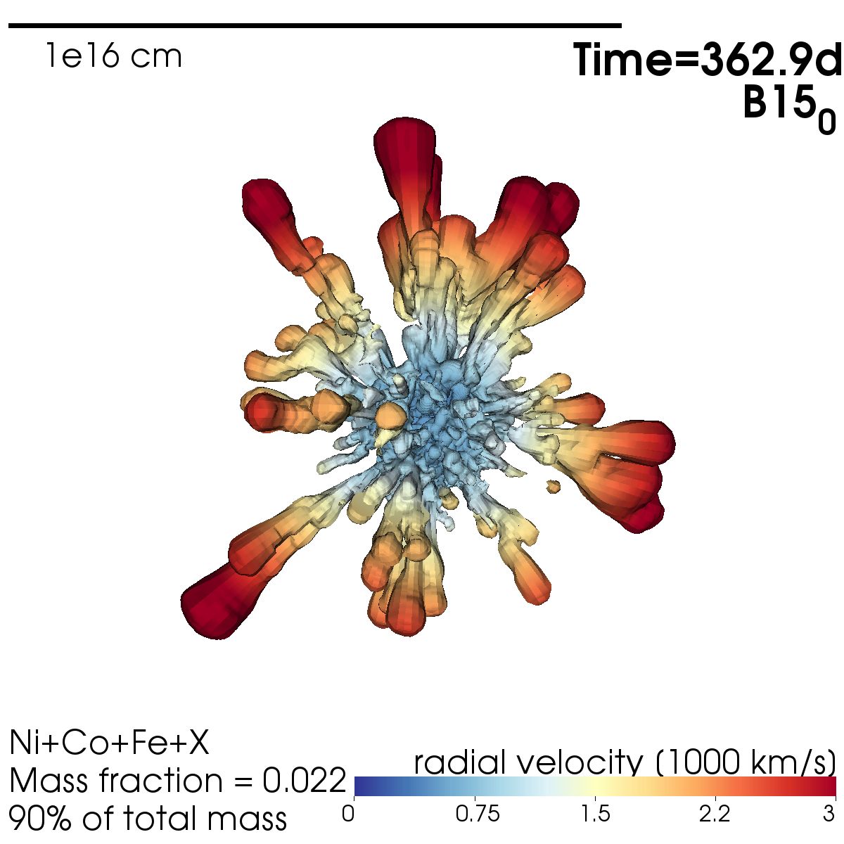
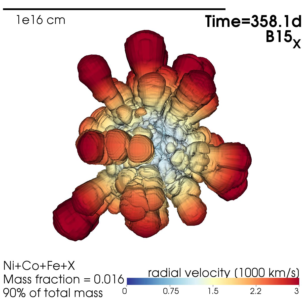
Figure 12: Isosurface plots of constant mass fraction of NiCoFeX for models B15₀, B15, and B15_X at $t\sim 1\,$d and $t\sim 1\,$yr, respectively. At $t\sim 1\,$d, all three models, B15₀ (top, left panel), B15 (top middle panel), and B15_X (top right panel), are almost indistinguishable because the $\beta$ decay did not significantly influence the evolution. After $t\sim 1\,$yr, the structures of B15₀ are almost the same as at $t\sim 1\,$d (compare upper and lower left panels), while the NiCoFeX-rich fingers of the other two models still inflate significantly after $t\sim 1\,$d. The final structures of model B15_X are more extended than those of model B15. The NiCoFeX mass fractions defining the isosurfaces are indicated in each panel.

In Fig. 12, we plot the models B15₀ (left), B15 (central) and B15_X (right) at two different times $t\sim 1\,$d (top row) and $t\sim 1\,$yr (bottom row). At $t\sim 1\,$d (top row) all three models have almost identical structures and the mass fraction thresholds are the same for all. This is expected since the only difference between the models is the treatment of the $\beta$ decay, which should not have any significant influence at this early time. At $t\sim 1\,$yr, the structures of the models B15 (bottom, central panel) and in particular B15_X (bottom, right panel) are significantly inflated. Model B15₀ is almost unchanged compared to $t\sim 1\,$d (left column). It also still has almost the same mass fraction threshold as in the beginning. The threshold $X_{\mathrm{NiCoFeX}}$ containing $90\%$ of the total mass of NiCoFeX of model B15 decreases from $0.023$ to $0.019$, and, due to the stronger inflation and the correspondingly stronger mixing, the one of B15_X decreases to $X_{\mathrm{NiCoFeX}}=0.016$.

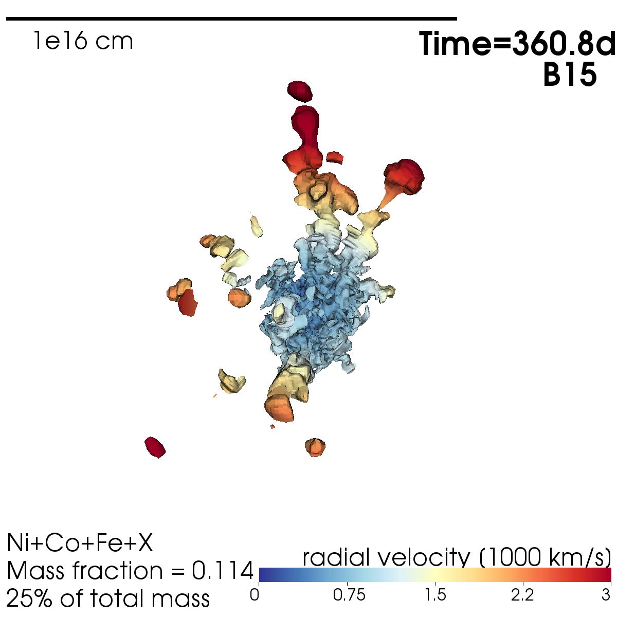
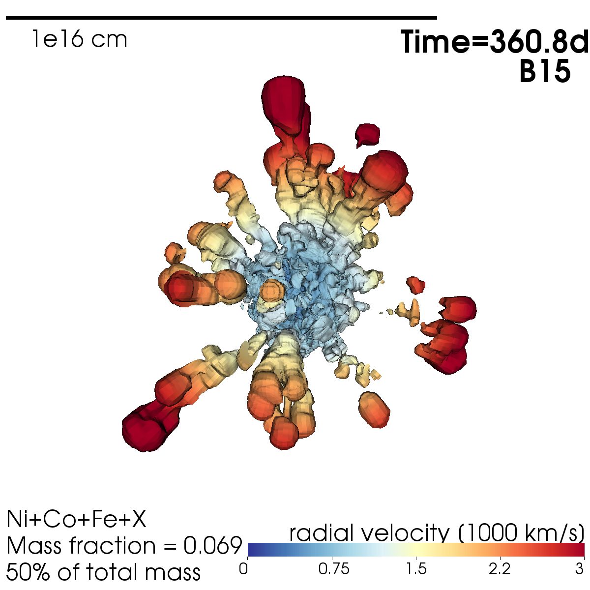
Figure 13: Isosurface plots of of constant mass fraction of NiCoFeX-rich ejecta containing different percentages of the total mass of these nuclei in model B15, from left to right $10\%$, $25\%$, and $50\%$, respectively. For lower percentages of the mass, more of the fingers disappear and mainly a central region with the highest mass fractions remains visible. The NiCoFeX mass fractions defining the isosurfaces are indicated in each panel.

In Fig. 13, we show the isosurfaces containing different mass percentages of NiCoFeX in the ejecta: $10\%$, $25\%$, and $50\%$, respectively. The morphologies are significantly different from each other depending on the mass fractions corresponding to the isosurfaces. In the left panel for $10\%$ of the NiCoFeX mass, the ejecta seem elongated preferentially along a particular axis. For the $25\%$ limit (central panel), the structures look similar, but there are additional small clumps distributed also on the left side of the image, while the right side is almost empty. Increasing to $50\%$ (right panel) more NiCoFeX-rich fingers and clumps appear. For a very low mass fraction threshold and, thus, for a plot that shows most of the NiCoFeX-rich ejecta like the third panel in Fig.11 for $90\%$, the fingers are more isotropically distributed. When comparing to observations, these significant differences should be kept in mind.

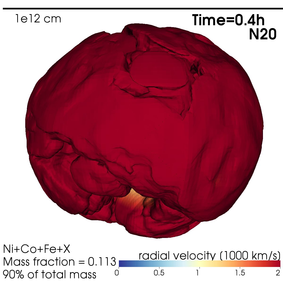
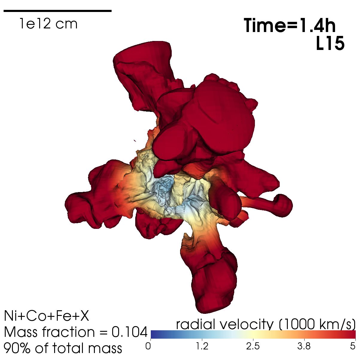
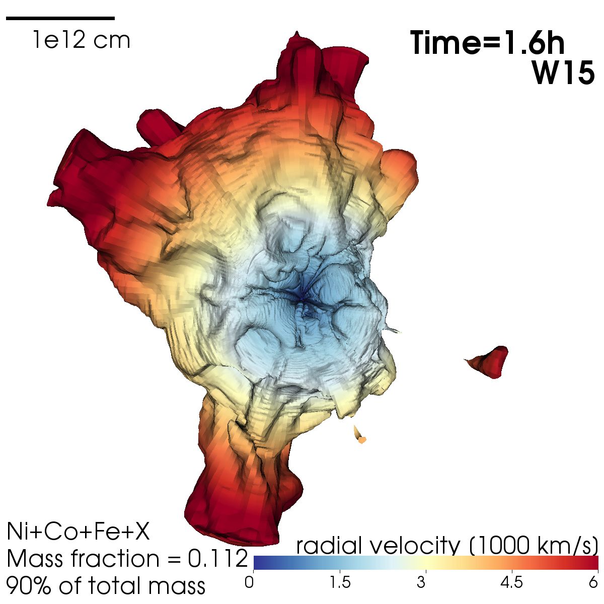
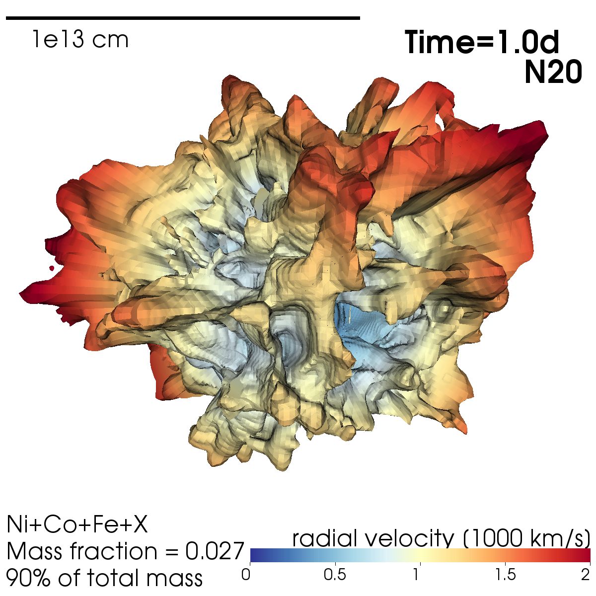
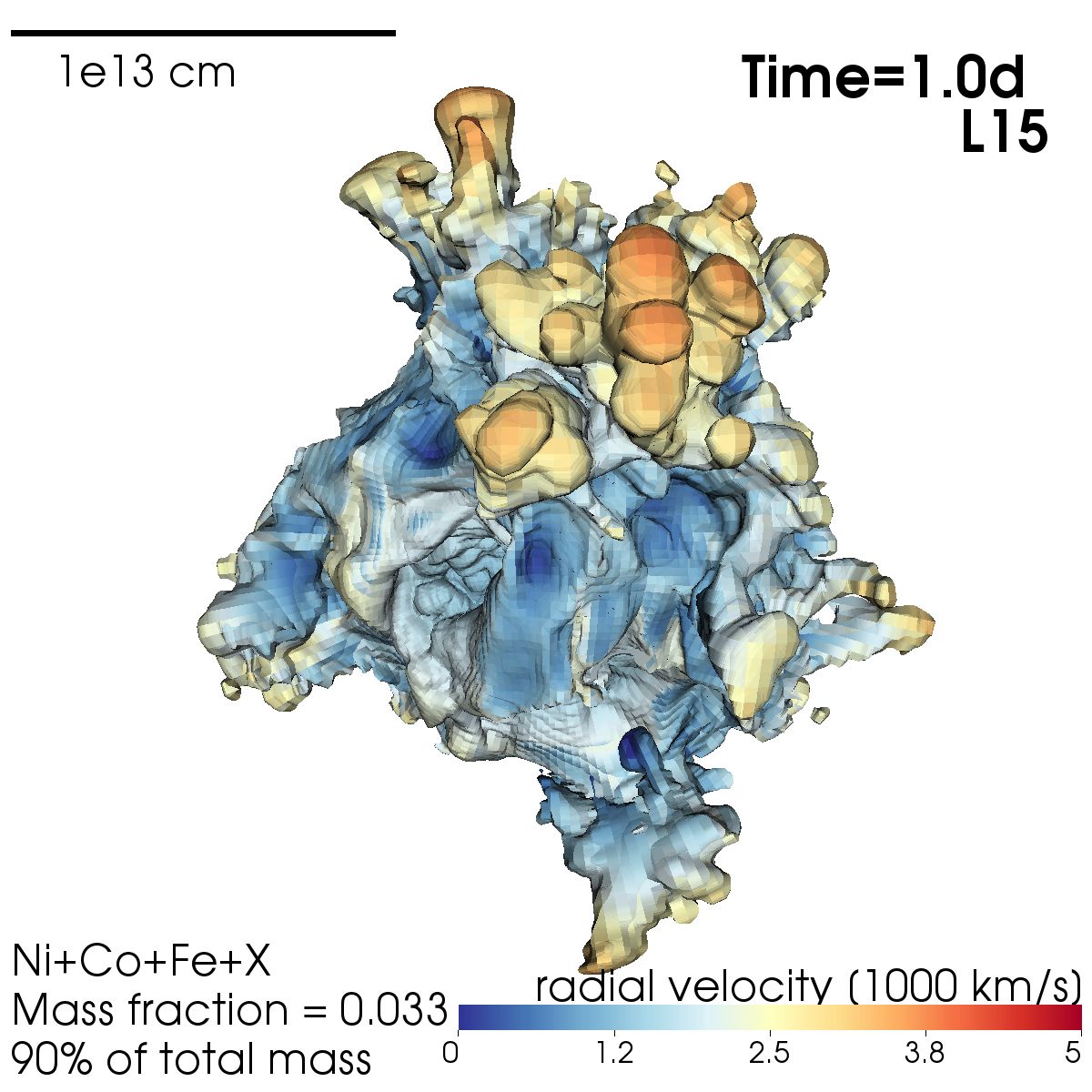
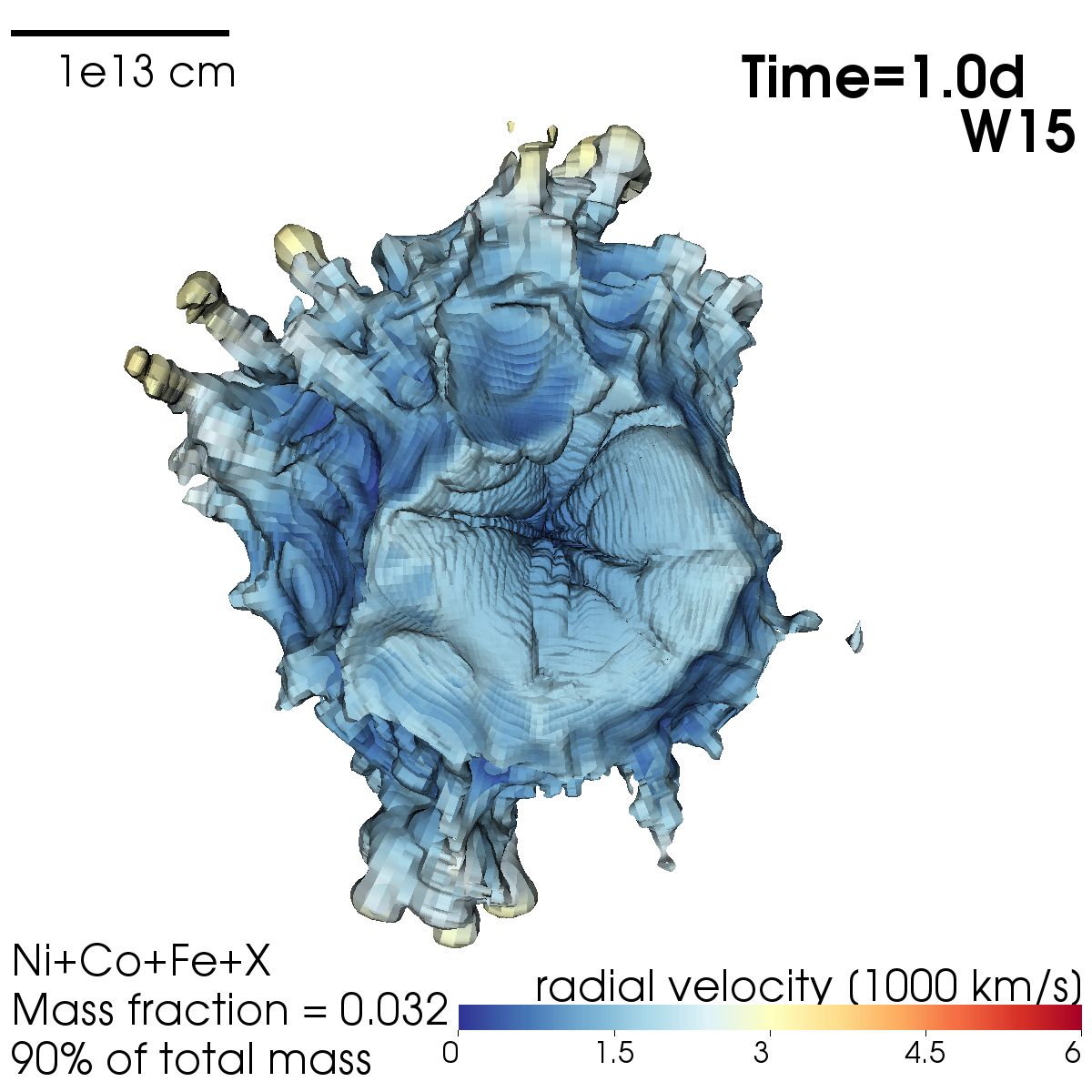
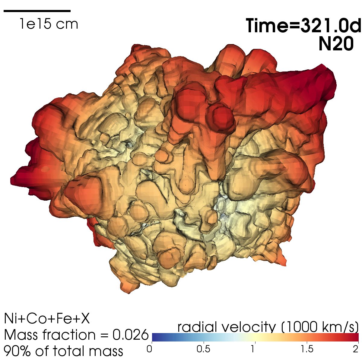
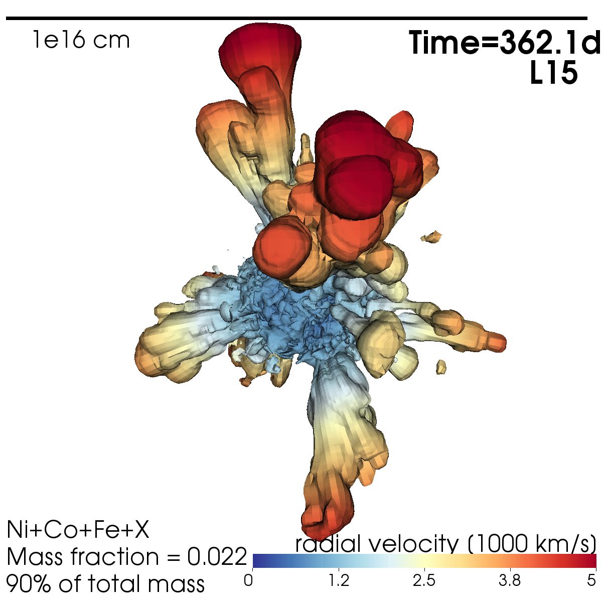
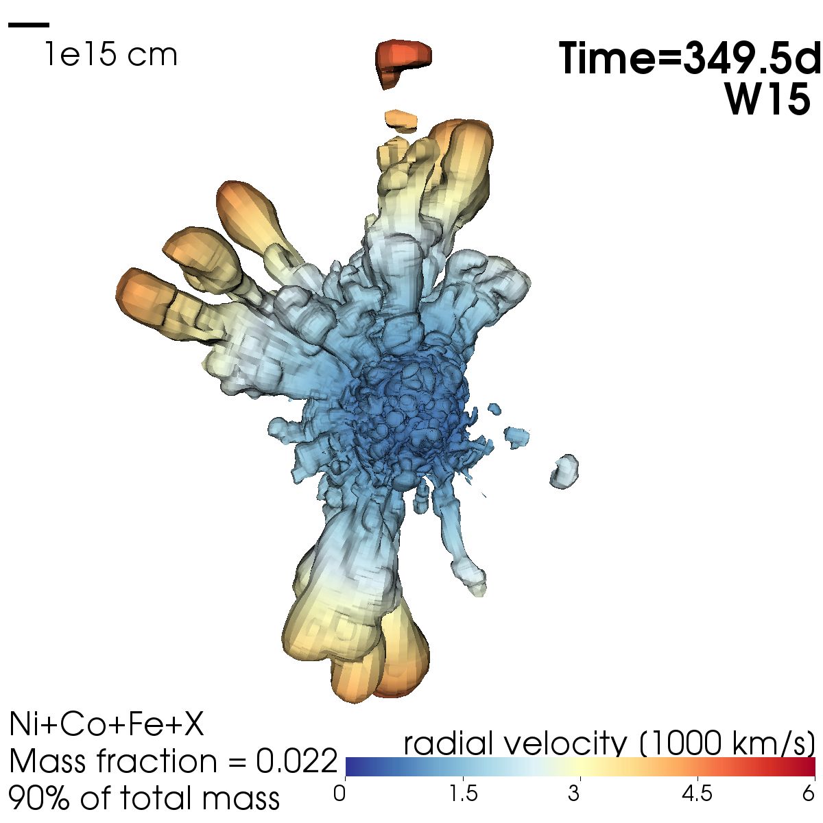
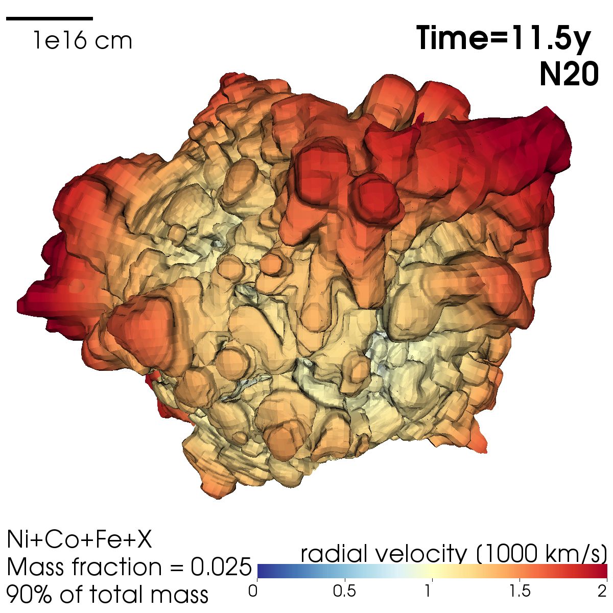
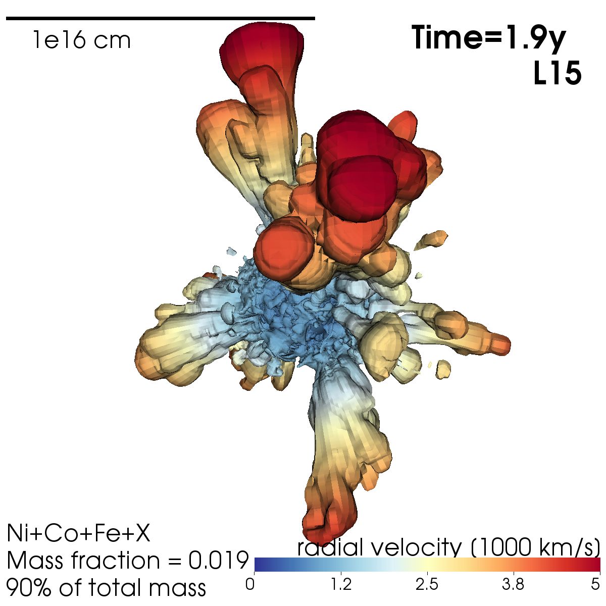
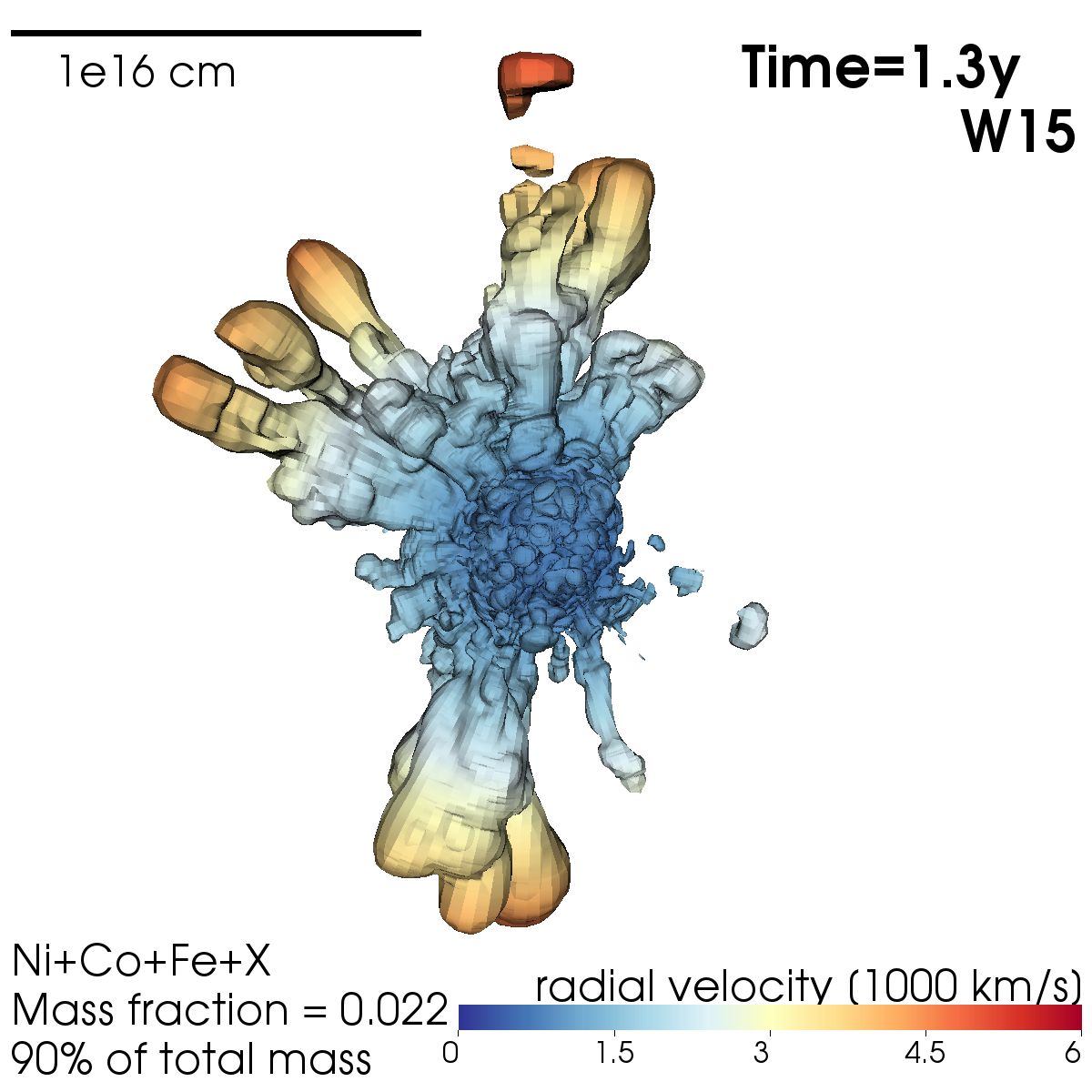
Figure 14: Isosurface plots of constant mass fraction containing $90\%$ of the mass of NiCoFeX in regions with highest mass fractions for different times and different models. Model N20 (left column) is almost spherical initially (top, left panel) and becomes slightly asymmetric after the shock breakout $t\sim 1\,$d (second row, left panel). These small asymmetries are then partially erased due to the inflation of the NiCoFeX-rich material. The two RSGs L15 (central column) and W15 (right column) are similar to each other. Initially at $t\gtrsim 1\,$h (top panels), they have large-scale plumes that fragment into smaller fingers (second and third row) and the reverse shock slows down the central ejecta compared to homologous expansion. A few strong NiCoFeX-rich clumps extend much farther out than the central bulk material. The decay of ⁵⁶Ni leads to an inflation of the central bubble and of the RT fingers. In all models, the structures no longer change significantly after $t\lesssim 1\,$yr (compare third and bottom row for the respective models). The NiCoFeX mass fractions defining the isosurfaces are indicated in each panel.

The NiCoFeX-rich structures of the other models are plotted in Fig. 14. The left column is for model N20, the central for L15 and the right for W15. The two RSG models L15 and W15 are qualitatively similar to each other, i.e. the initially large plumes (top central and right panels) fragment into smaller fingers due to RTIs, which occur during the SN shock propagation through the progenitor (see also Wongwathanarat et al., 2015, for a detailed discussion). The reverse shock begins to slow down the central ejecta compared to homologous expansion at about $t\sim 1\,$d (second row, central and right panels). Consequently, the central NiCoFeX-rich bubble shrinks relative to the extended fingers. Then, the reverse shock self-reflects and accelerates the innermost, central ejecta, supported by the input from the $\beta$-decay energy. Also the initially big, but later fragmented plumes inflate due to $\beta$ decay. After the fragmentation is finished, and the inflation due to $\beta$ decay becomes significant, these transiently fine-structured fingers merge to large-scaled clumps again, which have a similar shape compared to the initial plumes. They are even more prominent at this late time, because the innermost ejecta were decelerated by the reverse shock for some time and, thus, the velocity difference between the outermost RT fingers and the central ejecta is larger. The corresponding final structures after $t\sim 1\,$yr are shown in the third row (central and right panels) and at the end of our simulations in the bottom row.

The NiCoFeX-rich structures we find in model N20 (left column in Fig. 14) are qualitatively very different from the other models. Shortly before the shock breakout from the progenitor (top left panel), the NiCoFeX-rich ejecta are almost spherically symmetrically distributed. At about $t\sim 1\,$d the model becomes slightly more asymmetric (second row, left panel), but then the expansion of the NiCoFeX-rich ejecta leads to a more spherical configuration again (third row, left panel). No significant asymmetries or RT fingers can be found. As there is no significant difference between the corresponding plots of all models between the third and the bottom row of Fig. 14, which shows the last times simulated, we conclude that the evolution of the structures becomes homologous after about $t\lesssim 1\,$yr in all models.

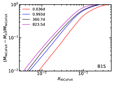
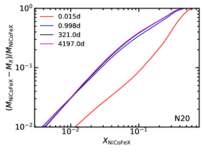
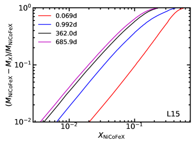
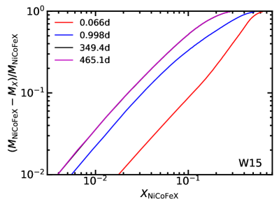
Figure 15: Fraction of mass of NiCoFeX $(M_{\mathrm{NiCoFeX}}-M_{X})/M_{\mathrm{NiCoFeX}}$ which has a smaller $X_{\mathrm{NiCoFeX}}$ than given at the corresponding x-coordinate for the different models at different times. Note that the black curves for models N20 and W15 are almost exactly covered by the magenta curves, indicating a perfectly homologous expansion between the corresponding last time steps.

To get a better feeling for the mass cut-offs applied to reach a certain fraction of the total mass $M_{X}/M_{\mathrm{NiCoFeX}}$ contained inside the isosurfaces defined by the minimal mass fractions $X_{\mathrm{NiCoFeX}}$ indicated in the plots, we provide the plots of the fraction of the mass $(M_{\mathrm{NiCoFeX}}-M_{X})/M_{\mathrm{NiCoFeX}}$ outside the corresponding isosurface as a function of $X_{\mathrm{NiCoFeX}}$ in Fig. 15 for the different models at different times. We choose to plot the complement to $M_{X}/M_{\mathrm{NiCoFeX}}$ for a better visualization of the fractions of the mass for small $X_{\mathrm{NiCoFeX}}$. The relatively large change at late times between the black and magenta curves for model B15 (top left panel) is related to the faster cut out of the central volume during the evolution. This did not influence the main results of the current work and was done for numerical efficiency as briefly described in Footnote 1.

3.3.5 Quantitative analysis

In the preceding sections, we described the structures obtained in the long-time evolution qualitatively. Here, we provide quantitative characteristics of the NiCoFeX-rich clumps for the different models. Since the particular choice of $F_{\rho}$ (or equivalently $\rho_{\mathrm{NiCoFeX}}^{\mathrm{min}}$) is somewhat arbitrary, we provide the characteristics of the clumps for different choices of $F_{\rho}$ for our models at $t\sim 1\,$yr in Table 4. The data in the table contain the minimal density $\rho^{\mathrm{min}}_{\mathrm{NiCoFeX}}$ above which we define the clump, the total number of clumps, the number of clumps with masses larger than $10^{-6}M_{\odot}$, and the volume of the clumps $V^{\mathrm{x}}_{\mathrm{NiCoFeX}}\equiv{V_{\mathrm{NiCoFeX}}}/{V_{\mathrm{x}}}$ compared to the volume of the sphere defined by the mean radius where the ejecta move with $\bar{v}_{1500}=1500\,$km/s, or $\bar{v}_{2500}=2500\,$km/s, respectively. The super- and subscripts $\mathrm{x}$ of $V^{\mathrm{x}}_{\mathrm{NiCoFeX}}$ or $V_{\mathrm{x}}$ represent the respective velocities. We also give the ratio of clump volume to the volume of the sphere defined by the radius of the fastest moving NiCoFeX. These fastest blobs are the outermost NiCoFeX-rich ejecta which have a mass fraction $X_{\mathrm{NiCoFeX}}>10^{-3}$. The corresponding maximal velocities $v_{\mathrm{fastest}}$ are given in Table 5. To have a measure to describe the clumpiness of the ejecta when 3D information in observations is not available, we provide the surface filling factors $A^{\mathrm{x}}_{\mathrm{NiCoFeX}}\equiv{A_{\mathrm{NiCoFeX}}}/{A_{\mathrm{x}}}$ of the corresponding clumps in the last three columns of Table 4. The reference line of sight to obtain the $A^{\mathrm{x}}_{\mathrm{NiCoFeX}}$ is in the y-direction such that we are looking at the x-z plane. This is the same viewing direction used in the Figs. 11 - 14.

Model	$F_{\rho}$	$\rho^{\mathrm{min}}_{\mathrm{NiCoFeX}}$	number	clumps with	$V_{\mathrm{NiCoFeX}}^{\mathrm{1500}}$	$V_{\mathrm{NiCoFeX}}^{\mathrm{2500}}$	$V_{\mathrm{NiCoFeX}}^{\mathrm{fastest}}$	$A_{\mathrm{NiCoFeX}}^{\mathrm{1500}}$	$A_{\mathrm{NiCoFeX}}^{\mathrm{2500}}$	$A_{\mathrm{NiCoFeX}}^{\mathrm{fastest}}$
		[g/cm3]	of clumps	$M>10^{-6}M_{\odot}$
B150	0.9	0.021	21	8	0.591	0.127	0.0349	0.799	0.562	0.232
	0.8	0.034	28	11	0.406	0.088	0.0240	0.693	0.483	0.198
	0.7	0.046	41	20	0.288	0.062	0.0170	0.592	0.407	0.166
	0.6	0.057	54	39	0.200	0.043	0.0118	0.514	0.338	0.136
	0.5	0.070	58	36	0.134	0.029	0.0079	0.441	0.264	0.105
	0.4	0.085	60	37	0.085	0.018	0.0050	0.372	0.193	0.075
	0.3	0.105	51	30	0.051	0.011	0.0030	0.294	0.129	0.049
	0.2	0.134	70	34	0.028	0.006	0.0017	0.202	0.081	0.029
	0.1	0.172	129	36	0.012	0.003	0.0007	0.125	0.046	0.017
B15	0.9	0.018	9	6	1.509	0.324	0.0866	0.952	0.721	0.305
	0.8	0.029	13	11	1.210	0.259	0.0694	0.912	0.674	0.283
	0.7	0.041	25	13	0.971	0.208	0.0557	0.864	0.624	0.259
	0.6	0.052	36	23	0.759	0.163	0.0436	0.790	0.565	0.231
	0.5	0.065	50	40	0.565	0.121	0.0324	0.715	0.490	0.199
	0.4	0.079	61	44	0.388	0.083	0.0223	0.643	0.402	0.160
	0.3	0.098	51	32	0.237	0.051	0.0136	0.554	0.300	0.116
	0.2	0.123	53	36	0.121	0.026	0.0070	0.409	0.181	0.066
	0.1	0.163	64	28	0.047	0.010	0.0027	0.268	0.100	0.036
B15X	0.9	0.016	5	3	3.154	0.643	0.1372	0.998	0.849	0.387
	0.8	0.025	9	5	2.755	0.562	0.1198	0.986	0.815	0.368
	0.7	0.039	18	10	2.386	0.487	0.1038	0.978	0.780	0.349
	0.6	0.044	23	11	2.011	0.410	0.0875	0.948	0.742	0.324
	0.5	0.055	39	24	1.616	0.330	0.0703	0.892	0.668	0.291
	0.4	0.068	63	39	1.200	0.245	0.0522	0.824	0.567	0.242
	0.3	0.085	77	43	0.792	0.161	0.0344	0.740	0.442	0.182
	0.2	0.107	71	35	0.423	0.086	0.0184	0.574	0.277	0.105
	0.1	0.145	91	28	0.151	0.031	0.0066	0.399	0.155	0.056
N20	0.9	0.026	5	2	0.766	0.163	0.1381	0.782	0.316	0.282
	0.8	0.047	7	2	0.607	0.129	0.1095	0.735	0.279	0.249
	0.7	0.071	6	3	0.488	0.104	0.0881	0.671	0.243	0.217
	0.6	0.100	23	4	0.396	0.084	0.0715	0.608	0.215	0.192
	0.5	0.138	25	1	0.315	0.067	0.0568	0.558	0.195	0.174
	0.4	0.180	32	3	0.243	0.052	0.0438	0.510	0.178	0.159
	0.3	0.228	36	8	0.175	0.037	0.0316	0.443	0.155	0.138
	0.2	0.280	51	13	0.110	0.024	0.0199	0.361	0.128	0.114
	0.1	0.333	37	17	0.051	0.011	0.0092	0.274	0.097	0.087
L15	0.9	0.021	31	13	2.534	0.527	0.0495	0.867	0.664	0.214
	0.8	0.037	35	21	1.822	0.379	0.0356	0.798	0.597	0.187
	0.7	0.052	62	37	1.378	0.287	0.0269	0.732	0.538	0.166
	0.6	0.068	51	28	1.056	0.220	0.0206	0.644	0.476	0.147
	0.5	0.085	58	30	0.798	0.166	0.0156	0.554	0.412	0.127
	0.4	0.102	54	27	0.588	0.122	0.0115	0.479	0.353	0.108
	0.3	0.121	72	32	0.398	0.083	0.0078	0.400	0.274	0.085
	0.2	0.143	116	46	0.230	0.048	0.0045	0.333	0.199	0.059
	0.1	0.175	125	59	0.084	0.018	0.0016	0.260	0.132	0.028
W15	0.9	0.022	20	8	1.451	0.307	0.0279	0.750	0.523	0.167
	0.8	0.039	25	17	0.974	0.206	0.0187	0.688	0.443	0.125
	0.7	0.057	20	12	0.698	0.148	0.0134	0.646	0.388	0.103
	0.6	0.074	42	22	0.500	0.106	0.0096	0.601	0.341	0.085
	0.5	0.093	61	34	0.354	0.075	0.0068	0.555	0.294	0.069
	0.4	0.113	60	28	0.238	0.050	0.0046	0.501	0.238	0.053
	0.3	0.137	78	34	0.152	0.032	0.0029	0.421	0.184	0.039
	0.2	0.167	95	29	0.088	0.019	0.0017	0.328	0.128	0.026
	0.1	0.208	130	30	0.040	0.008	0.0007	0.230	0.082	0.017

Table 4: Characteristics of the clumps of NiCoFeX after $t\sim 1\,$yr for models B15₀, B15, B15_X, N20, L15, and W15, respectively. In the different columns we give the model name, the fraction of mass of the clumps compared to the total mass of NiCoFeX, $F_{\rho}$ , the threshold density above which we define the clumps, the number of clumps, the number of clumps with NiCoFeX mass larger than $10^{-6}M_{\odot}$, the volume of the clumps compared to the volumes inside a sphere with the radius where the mean velocities of the material are $\bar{v}_{1500}=1500\,$km/s, $\bar{v}_{2500}=2500\,$km/s, and $v_{\mathrm{fastest}}^{\mathrm{NiCoFeX}}$, and finally the surface area in the x-z plane covered by the NiCoFeX clumps compared to a square with side length of twice the radius where the ejecta move with $\bar{v}_{1500}$, $\bar{v}_{2500}$, and $v_{\mathrm{fastest}}^{\mathrm{NiCoFeX}}$, respectively.

Model	B150	B15	B15X	N20	L15	W15
$v^{\mathrm{NiCoFeX}}_{\mathrm{fastest}}$ [km/s]	3813	3899	4199	2646	5484	5544
$r^{\mathrm{NiCoFeX}}_{\mathrm{fastest}}$	12.0	12.1	12.8	7.3	17.1	16.7
[$10^{15}$cm]

Table 5: Velocity $v_{\mathrm{fastest}}^{\mathrm{NiCoFeX}}$ and radius of the fastest NiCoFeX at $t\sim 1\,$yr. The minimum mass fraction to define the fastest NiCoFeX is $10^{-3}$.

As expected, there are more clumps when the density threshold is increased. For low densities $\rho^{\mathrm{min}}_{\mathrm{NiCoFeX}}$, large volumes are connected and form big clumps. If the threshold for the definition of the clump is increased, different high-density ‘islands’ get disconnected from each other and form separate clumps. However, as a secondary effect some clumps disappear completely because their highest density of NiCoFeX elements falls below the selected threshold. For example see model B15₀ or B15, where the number of clumps decreases despite an increase of $\rho^{\mathrm{min}}_{\mathrm{NiCoFeX}}$ from $F_{\rho}=0.4$ to $F_{\rho}=0.3$. For the volume and surface filling factors, we see a monotonic trend of decreasing values with increasing density threshold for all models. Note that we allow for volume filling factors larger than one, which states that the NiCoFeX-rich ejecta fill a larger volume than that given by a sphere of a particular radius. For model B15, $\bar{v}_{1500}$ and $F_{\rho}=0.9$, we find $V_{\mathrm{NiCoFeX}}^{\mathrm{1500}}=1.509$, which means that significant parts of the NiCoFeX-rich ejecta move faster than $\bar{v}=1500\,$km/s.

Let us compare the different prescriptions for the $\beta$ decay in model B15. The density threshold of the clumps containing $90\%$ of the NiCoFeX mass decreases from $\rho^{\mathrm{min}}_{\mathrm{NiCoFeX}}=0.021\,$g/cm³ for B15₀ to $\rho^{\mathrm{min}}_{\mathrm{NiCoFeX}}=0.018\,$g/cm³ for B15 and finally to $\rho^{\mathrm{min}}_{\mathrm{NiCoFeX}}=0.016\,$g/cm³ for B15_X. This decrease has two main reasons: the extra mixing in particular at the finger borders caused by instabilities due to the inflation (see also Basko, 1994; Blondin et al., 2001; Chevalier, 2005), and the reduction of the densities inside the NiCoFeX-rich ejecta due to the inflation. The same trend of decreasing densities with stronger $\beta$ decay holds for all fractions of the total NiCoFeX mass, B15₀ has always the highest and B15_X the lowest $\rho^{\mathrm{min}}_{\mathrm{NiCoFeX}}$. The number of clumps is also related to the inflation of the clumps. The more the initially separated clumps inflate, the more of the clumps merge. For $F_{\rho}=0.9$, there are 21 clumps for B15₀, 9 clumps for B15, and only 5 clumps for B15_X. The opposite trend holds for the respective volume and area filling factors. The stronger the $\beta$ decay is, the larger are the filling factors $V_{\mathrm{NiCoFeX}}^{\mathrm{x}}$ and $A_{\mathrm{NiCoFeX}}^{\mathrm{x}}$. This is expected because the inflation leads to an increase of volume and area.

Model N20 has the smallest number of individual clumps. This can already be seen in Fig. 14, where this model is the most spherically symmetric. It is also the only model without significantly extended NiCoFeX-rich fingers. Therefore, all ejecta are at comparable radii and one big central bubble dominates. When increasing the density threshold only a small number of clumps show up. The two RSG models L15 and W15 have comparable numbers of clumps, which are significantly larger than the one for model N20. The NiCoFeX-rich fingers in Fig. 14 extend to larger radii than the bulk of the material. These fast ejecta form many separated clumps when the density threshold is increased, and the structures get disconnected from the central bubble. Model B15 has an intermediate number of clumps.

Among the models with standard $\beta$ decay, model L15 has volume filling factors for $\bar{v}_{1500}$ and $\bar{v}_{2500}$ that are at least $50\%$ higher than those of all other models (B15, N20, W15). $V_{\mathrm{NiCoFeX}}^{\mathrm{fastest}}$ seems not to follow the same trend, however, remember that each model has a different value of $v_{\mathrm{fastest}}$, see Table 5. Compared to models B15 and N20, which have larger $V_{\mathrm{NiCoFeX}}^{\mathrm{fastest}}$, model L15 has the fastest moving NiCoFeX, and, hence, the volume of the sphere with the corresponding radius is the largest among these models. So despite of having the largest $V_{\mathrm{NiCoFeX}}^{\mathrm{1500}}$ and $V_{\mathrm{NiCoFeX}}^{\mathrm{2500}}$, model L15 does not have the largest $V_{\mathrm{NiCoFeX}}^{\mathrm{fastest}}$. In Table 5, we note that the velocity of the fastest moving ejecta of model W15 is even slightly faster than that of model L15, which seems to contradict our discussions related to Tables 3 and 3. However, in those tables we considered the mean velocities of the bulk and of the fastest one percent of the ejecta. Here, we take the absolute value of the velocity of the very fastest ejecta having $X_{\mathrm{NiCoFeX}}>10^{-3}$, which make up less than $10^{-6}$ of the total NiCoFeX-mass only.

The surface filling factors of all the models are more similar to each other. Model B15 has the largest values for $A_{\mathrm{NiCoFeX}}^{\mathrm{1500}}$ and $A_{\mathrm{NiCoFeX}}^{\mathrm{2500}}$. The different behaviour of the 2D projections and 3D analysis can be explained by the different morphologies of the models: The NiCoFeX-rich clumps and fingers of model B15 are distributed more isotropically than in the other models (see Figs. 11 and 14). In a surface projection, this leads to almost complete coverage of the entire surface within a square of side length $2\times r_{1500}$. Models L15 and W15, which only have a few NiCoFeX-rich fingers in distinct directions, only have $A_{\mathrm{NiCoFeX}}^{\mathrm{1500}}\simeq 0.87$ and $0.75$ for $F_{\rho}=0.9$, respectively. The large volume filling factor of L15 can be explained by the few large fingers that extend to very large radii compared to the central bubble of the NiCoFeX-rich ejecta. The fingers of model B15 are less extended and, hence, the volume filled by these structures is comparably smaller than those in model L15. Without any extended NiCoFeX-rich fingers, model N20 has the smallest $V_{\mathrm{NiCoFeX}}^{\mathrm{1500}}$ and $V_{\mathrm{NiCoFeX}}^{\mathrm{2500}}$ of all models with standard $\beta$ decay. Again, $V_{\mathrm{NiCoFeX}}^{\mathrm{fastest}}$ does not follow this trend because the $v_{\mathrm{fastest}}$ are different for all models. As for the volume filling factors, model N20 has also the smallest surface filling factor $A_{\mathrm{NiCoFeX}}^{\mathrm{2500}}$. However, the surface filling factor for $\bar{v}_{\mathrm{1500}}$ is not following this trend. $A_{\mathrm{NiCoFeX}}^{\mathrm{1500}}$ is slightly larger for model N20 than that for model W15 for all $F_{\rho}$. The larger occupied surface area shows that the fastest ejecta of the central spherical bubble of model N20 is moving faster than that of model W15 (see also Fig. 7), and that this difference cannot be cured by the few extended and fast-moving NiCoFeX-rich fingers. Note that the volume and surface filling factors $V_{\mathrm{NiCoFeX}}^{\mathrm{1500}},V_{\mathrm{NiCoFeX}}^{\mathrm{2500}},A_{\mathrm{NiCoFeX}}^{\mathrm{1500}}$, and $A_{\mathrm{NiCoFeX}}^{\mathrm{2500}}$ depend sensitively on the explosion energy of the model. The higher the explosion energy is, the faster the ejecta should propagate and, hence, the larger the filling factor for the volumes and surfaces determined by fixed velocities should be after $1\,$yr. Only the entries compared to the fastest moving NiCoFeX-rich ejecta, $V_{\mathrm{NiCoFeX}}^{\mathrm{fastest}}$ and $A_{\mathrm{NiCoFeX}}^{\mathrm{fastest}}$, should be less sensitive to the particular value of the explosion energy, since in this case $v_{\mathrm{fastest}}$ also scales with the explosion energy.

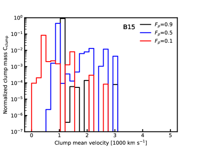
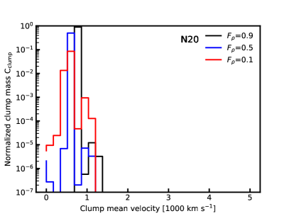
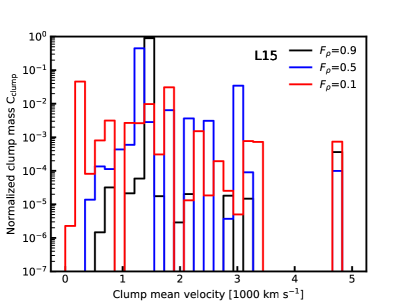
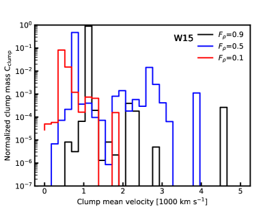
Figure 16: Distributions $C_{\mathrm{clump}}$ of the normalized mass in clumps with a given mean velocity $\bar{v}_{\mathrm{clumps}}$ containing $90\%$, $50\%$, and $10\%$ of the ejecta with the highest densities of NiCoFeX for models B15 (top left panel), N20 (top right panel), L15 (bottom left panel), and W15 (bottom right panel), respectively. The normalization is relative to the total NiCoFeX mass. When considering $90\%$ of the NiCoFeX mass ($F_{\rho}=0.9$), almost all material is concentrated in one central bubble with mean clump velocity of approximately $\bar{v}\sim 1000\,$km/s for all models. When reducing $F_{\rho}$ and, consequently, increasing the density threshold, the main bubble shifts to lower velocities, and clumps at different mean clump velocities disconnect from the central bubble. Due to the little mixing and weak self-reflected shock, model N20 has the slowest clumps. The bins of the mean velocity have a width of $167\,$km/s.

When considering the clumps as completely disconnected, we can define a mean velocity for each individual clump $\bar{v}_{\mathrm{clump}}$:

$$\bar{v}_{\mathrm{clump}}=\frac{\int\limits_{\mathrm{clump}}\rho vdV}{M_{\mathrm{clump}}}\,.$$ (16)

To see how many clumps and also how much mass propagate with a certain velocity, we plot the mass inside the clumps normalized to the total NiCoFeX mass

$$C_{\mathrm{clump}}(\bar{v}_{\mathrm{clump}})\equiv\frac{M_{\mathrm{clump}}(\bar{v}_{\mathrm{clump}})}{M^{\mathrm{tot}}_{\mathrm{NiCoFeX}}}\,,$$ (17)

as a function of $\bar{v}_{\mathrm{clump}}$ in Fig. 16. Here, $M_{\mathrm{clump}}(\bar{v}_{\mathrm{clump}})$ is the NiCoFeX mass of the clumps with mean velocity $\bar{v}_{\mathrm{clump}}$, and $M^{\mathrm{tot}}_{\mathrm{clumps}}$ is the total NiCoFeX mass (including the NiCoFeX not contained in the clumps). If more than one clump falls within the same velocity bin, we add up the normalized masses of these clumps. For the central bubble, i.e. the ‘clump’ with the largest $C_{\mathrm{clump}}$, the latter is not a useful measure. For large $F_{\rho}$, the central ejecta can be very extended and be connected to very elongated NiCoFeX-rich fingers. Consequently, the integral in Eq. (16) gives essentially the bulk velocity of the NiCoFeX elements.

Comparing $C_{\mathrm{clump}}$ for $F_{\rho}=0.9$ (black curve, top left panel of Fig. 16) and $F_{\rho}=0.5$ (red) of model B15, we see that there are more clumps with higher velocities for $F_{\rho}=0.5$. The big central ejecta bubble at $\bar{v}_{\mathrm{clump}}\gtrsim 1000\,$km/s for $F_{\rho}=0.9$ splits into many smaller clumps for $F_{\rho}=0.5$, some with higher velocities, but there are also more clumps with lower velocities $\bar{v}_{\mathrm{clump}}<1000\,$km/s. The mean velocity of the central bubble reduces from $\bar{v}_{\mathrm{clump}}\gtrsim 1000\,$km/s for $F_{\rho}=0.9$ (black line) to $\bar{v}_{\mathrm{clump}}\lesssim 1000\,$km/s for $F_{\rho}=0.5$ (red line) to $\bar{v}_{\mathrm{clump}}\lesssim 500\,$km/s for $F_{\rho}=0.1$ (blue line). This decrease of the mean velocity is a consequence of the fragmentation of the big central clump. The still connected part of the central ejecta shrinks and has higher densities. Since this means considering denser material farther inside, the mean velocity of these ejecta decreases compared to those of a more extended central bubble for $F_{\rho}=0.9$. Similar trends are found for all models shown in the other panels of Fig. 16.

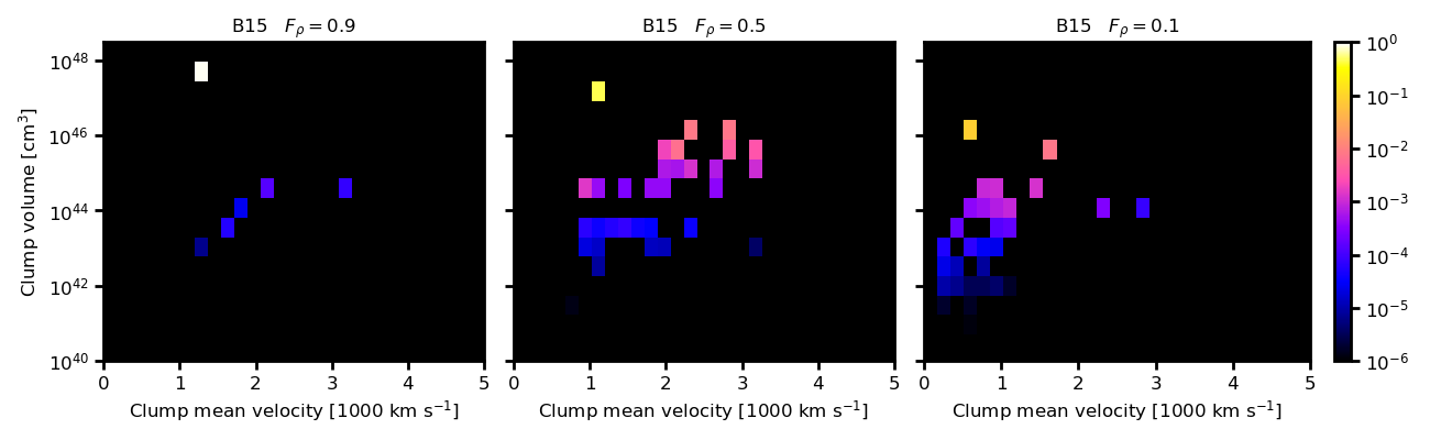
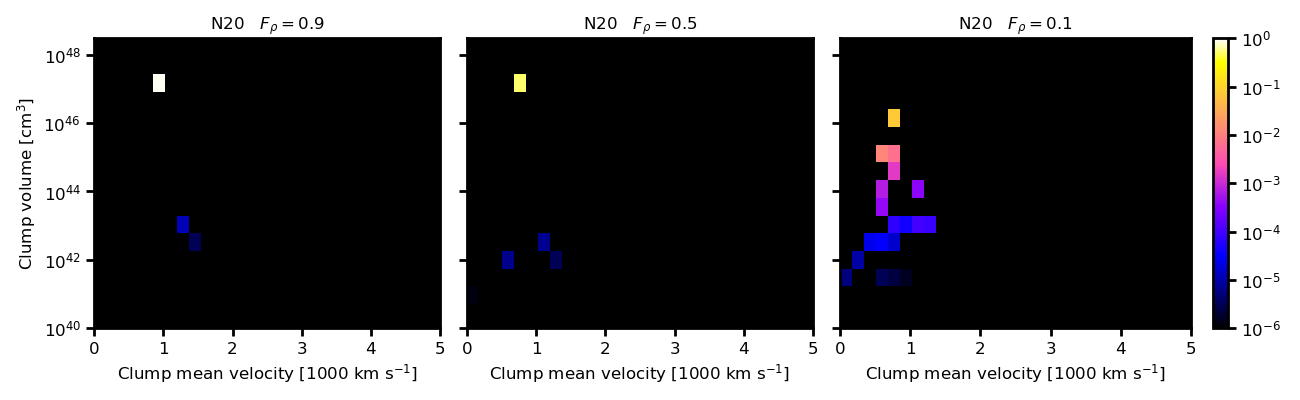
Figure 17: Pseudocolour plots of the mass in individual clumps normalized by the total mass of NiCoFeX as function of the clump velocity (x-axis), and clump volume (y-axis) for different models. We assume that the clumps contain the densest NiCoFeX material and their mass sums up to different fractions of the total mass of NiCoFeX: $90\%$ (left column), $50\%$ (central column), and $10\%$ (right column). If more than one clump falls within the same velocity and volume bin, we add up the normalized masses of these clumps. When considering the densest $90\%$ ($F_{\rho}=0.9$), all models have a dominant clump (the central bubble) in volume and fractional mass around $\bar{v}\sim 1000\,$km/s, visible as the white or yellow squares in the top left corner of the panels. Model N20 (second row) has the fewest number of clumps followed by model B15 (top row). The two RSG models L15 (third row) and W15 (bottom row) have more clumps with a wider spread in velocity. Considering $F_{\rho}=0.5$, the large central bubble fragments and smaller clumps get disconnected for all models. This fragmentation results in a wide distribution of clump sizes and velocities. This also happens when lowering $F_{\rho}$ to $0.1$. However, in this case many clumps also disappear, because their densities fall below the corresponding threshold (see in particular model W15 central and right lower panels). The largest dispersion of sizes and clumps is found for model L15 (third row). The binning in velocity is $167\,$km/s, the logarithmic bin width in volume is $0.5\log(\mathrm{cm}^{3})$, and the colour scale of the normalized mass in the clumps is logarithmic.

The fastest clumps of model N20 do not exceed velocities $\bar{v}_{\mathrm{clump}}\lesssim 1500\,$km/s. The fastest clumps with $\bar{v}_{\mathrm{clump}}>4000\,$km/s are found for models L15 and W15. However, these fast clumps contain very little mass ($<10^{-3}$ of the total mass). Comparing the normalized masses of the clumps of models L15 (bottom left panel) and W15 (bottom right panel), we find that for $F_{\rho}=0.9$ (black lines) the distributions look quite similar, with a main peak around $1000\mathrm{~{}km/s}<\bar{v}_{\mathrm{clump}}<1500\mathrm{~{}km/s}$, a wide spread of mean clump velocities up to $\bar{v}_{\mathrm{clump}}\lesssim 3000\,$km/s, and one very fast clump. Also, $\bar{v}_{\mathrm{clump}}$ of the densest $50\%$ of the NiCoFeX ejecta decrease in both cases (blue lines). However, considering only the densest $10\%$, the distribution of normalized clump mass as a function of velocity of model W15 is very narrow and constrained to low velocities $0<\bar{v}_{\mathrm{clump}}<2000\,$km/s. In contrast, model L15 still has a very broad distribution of velocities for its densest clumps.

In Fig. 17, we combine the information about the size of the clumps (y-axis), the mean clump velocities (x-axis) and the mass contained in the clumps. The colour scale represents the NiCoFeX mass of a clump at the given velocity and for a given volume, normalized by the total mass of NiCoFeX of the simulation. If more than one clump falls within the same velocity and volume bin, we add up the normalized masses of these clumps. As expected, the central ejecta bubble (white or yellow squares in the top left corner of the panels) is always dominant in volume and mass fraction. For $F_{\rho}=0.9$, we see only a few clumps apart from the central ejecta. In general, models W15 and L15 have more clumps than B15, and model N20 has the smallest number of clumps (this actually holds for all density thresholds). The spread in clump sizes is comparable in all models, while the spread in velocity is significantly smaller for model N20 compared to the other models. As noted before, for the $10\%$ of the densest NiCoFeX clumps, model L15 has the largest velocity spread, while at $F_{\rho}=0.9$ the spreads of models B15, L15, and W15 are comparable. Apart from model N20, the clump volume is correlated with the mean clump velocity as is most apparent in the third and fourth rows of the central column. This means that there is a general trend that the biggest clumps (apart from the central bubble) have the highest velocities, which makes sense because the fastest clumps have expanded most. However, due to their lower densities the fastest clumps do not necessarily have the highest clump masses.

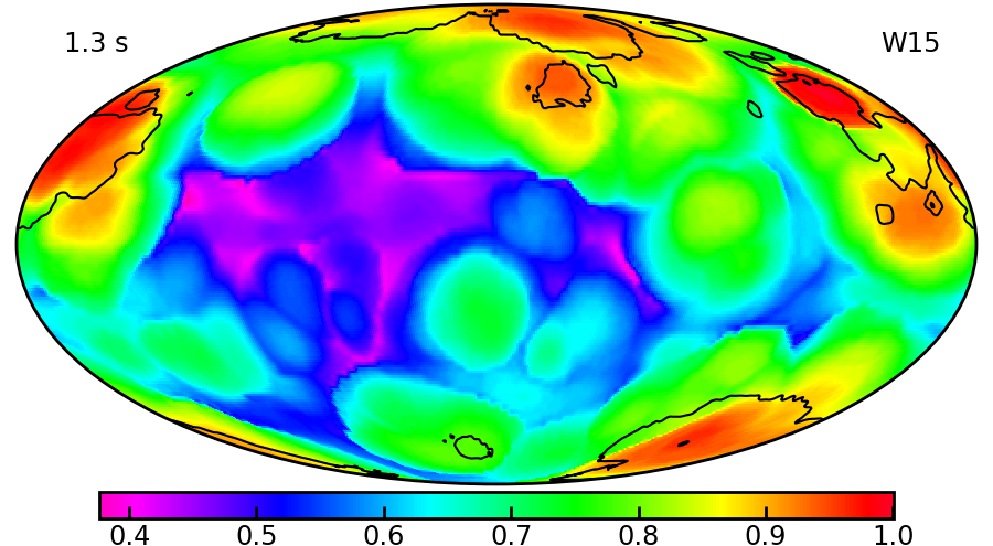
Figure 18: Colour coded are the Mollweide projections of the normalized maximal radii $R^{56}_{\mathrm{max}}(\theta,\phi)/R^{\mathrm{tot}}_{\mathrm{max}}$ at $t\sim 1-2\,$s, where $R^{56}_{\mathrm{max}}(\theta,\phi)$ is defined at $X_{\mathrm{NiFoFeX}}>10^{-3}$ and $R^{\mathrm{tot}}_{\mathrm{max}}=\max\left(R^{56}_{\mathrm{max}}(\theta,\phi)\right)$ of all directions $(\theta,\phi)$. The black contour lines are the locations where $R^{56}_{\mathrm{max}}(\theta,\phi)=0.5R^{\mathrm{tot}}_{\mathrm{max}}$ at $t\sim 1\,$yr. The most prominent structures of models B15, L15, and W15 are in the same directions at early and late times. Model N20 is an exception and does not exhibit any tight correlation between the biggest initial and final structures, because its initial nickel plumes are efficiently decelerated by the reverse shock and therefore not able to penetrate deep into the hydrogen envelope. Instead, they fragment into smaller-scale structures growing from RT instability at the He/H interface.

3.3.6 Comparison with initial explosion asymmetries

The final asymmetries, in particular the biggest structures, in the iron distribution are clearly linked to the biggest initial bubbles of neutrino-heated ejecta created at the onset of the explosion. This can be seen by comparing the isosurface plots of the NiCoFe-rich ejecta at early times in the left column of panels of figure 7 of Wongwathanarat et al. (2015) to the late times in Figs. 11 and 14. The fastest plumes shaped by the buoyant rise of neutrino-heated matter in the initial moments of the explosion end up as the biggest extended fingers or clumps at late times.

To emphasize the correlation between the initial and final asymmetries further, we plot the Mollweide projections of the maximal radius $R^{56}_{\mathrm{max}}(\theta,\phi)$ in a given direction $(\theta,\phi)$ at the time of shock revival compared to the corresponding radius at $t\sim 1\,$yr in Fig. 18. Remember that $R^{56}_{\mathrm{max}}(\theta,\phi)$ was defined as the outermost radius where $X_{\mathrm{NiFoFeX}}>10^{-3}$. For the color-coding we rescaled the $R^{56}_{\mathrm{max}}(\theta,\phi)$ by the maximal $R^{56}_{\mathrm{max}}(\theta,\phi))$ of all directions $(\theta,\phi)$, $R^{\mathrm{tot}}_{\mathrm{max}}=\max\left(R^{56}_{\mathrm{max}}(\theta,\phi)\right)$, at the indicated times $t\sim 1-2\,s$. The black contour lines are the locations where $R^{56}_{\mathrm{max}}(\theta,\phi)=0.5R^{\mathrm{tot}}_{\mathrm{max}}$ at $t\sim 1\,$yr. These contour lines coincide almost perfectly with the highest amplitudes represented by yellow and red colours for models B15, L15, and W15. This correlation demonstrates that the most extended structures at $t\sim 1-2\,$s are in the same directions as the most prominent features at $t\sim 1\,$yr. Model N20, which does not have very extended structures, shows no clear correlations between the initial and the late time asymmetries.

3.3.7 Spherical harmonics decomposition

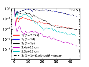
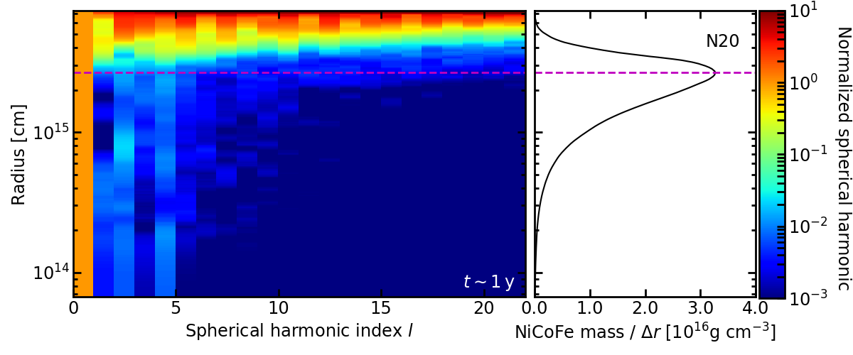
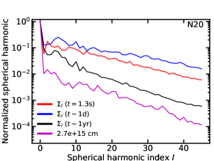
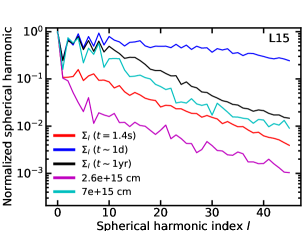
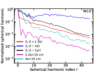
Figure 19: Spherical harmonics decomposition of the linear momentum of NiCoFe-rich matter in radial direction of the clumps containing $90\%$ of the densest material of NiCoFe for different models B15 (top row), N20 (second row), L15 (third row), and W15 (bottom row). Left column: Spherical harmonic coefficients at a given radius normalized to the monopole as a function of $r$ and multipole order $l$ at $t\sim 1\,$yr. Central column: Mass of NiCoFe per unit length scale as a function of radius. Right column: Normalized spherical harmonics coefficient at the radii given by the horizontal dashed lines in the left and central panels with the same colour. The blue and black lines represent the sum of the coefficients $c_{l}$ over all radial cells $\Sigma_{l}$ at $t\sim 1\,$yr, $t\sim 1\,$d and at the indicated times (which are approximately the first times given in figure 7 of Wongwathanarat et al., 2015), respectively. All models have a dominant monopole representing the bulk of the material that is ejected nearly spherically. The most spherical model N20 has very weak higher multipoles and is dominated by the monopole everywhere, where most of the mass of NiCoFe is located ($r\lesssim 5\times 10^{15}\,$cm). Model B15 has many, almost isotropically distributed RT fingers extending to large radii, explaining the high contribution of the spherical harmonics around $l=10$ (top right panel). The RSG models have only a few, but quite extended fingers leading to a strong quadrupole ($l=2$) and hexadecapole ($l=4$) asymmetry for model L15 (third row, right panel) and a strong dipole ($l=1$) and quadrupole ($l=2$) asymmetry for W15 (bottom right panel).

To further analyse the spatial distribution of the NiCoFe-rich ejecta, we decompose the linear momentum of NiCoFe-rich matter in the radial direction of the models into spherical harmonics. The corresponding plots of the decomposition normalized to the monopole and for each radius of our numerical grid are displayed in the left column of panels in Fig. 19. To obtain a measure where most of the mass of the NiCoFe-rich ejecta is located we plot the mass of NiCoFe inside shells divided by the radial width of the corresponding shells, in the central column of panels. We mark the maximum with a magenta dashed line in each panel of the left and central columns. For all of our models, the monopole dominates at small radii $r\lesssim\mathrm{few}\times 10^{15}\,$cm, including the radius containing the mass maximum. The dominating monopole at low radii can also be seen clearly in the right column of panels, where we plot the spherical harmonics decomposition at the radius of the mass maximum (magenta solid line). In all models the monopole is at least one order of magnitude larger than the dipole component.

When increasing the radius above $r\gtrsim\mathrm{4}\times 10^{15}\,$cm, we find that higher multipoles become more and more important and start to dominate close to the fastest moving NiCoFe-rich ejecta at the top of each of the left panels. However, the mass in the topmost region in the plots is negligible. We thus plot an additional line at large, but not too large radii, which contains the main asymmetries of the explosions in the NiCoFe-rich fingers (dashed and solid cyan lines in the central and right panels of Fig. 19). We choose the radius at the locations where we see a slight bump of the $M_{\mathrm{NiCoFe}}/\Delta r$ distributions in the corresponding plots in the central panels. Note that for model N20 due to the absence of extended RT fingers, there is no interesting region apart from the maximum of the $M_{\mathrm{NiCoFe}}/\Delta r$ distribution. For large radii the decompositions for the different models have different characteristics. Model N20 is dominated by the monopole at all radii where significant mass is located, while the other models start to have also significant contributions from higher multipoles. For model W15 (bottom row, right panel), the dipole at $r\sim 4\times 10^{15}\,$cm is even stronger than the monopole ($l=0$), and model L15 (third row) has very strong quadrupole ($l=2$) and hexadecapole ($l=4$) components. These structures are also confirmed in the corresponding plots at late times in Fig. 14 (third and fourth row, central and right panels). In Fig. 11, we see that model B15 has many more NiCoFe-rich fingers, and this also reflects in the spherical harmonics decomposition. We find a strong quadrupole contribution, but in contrast to all other models, we also find a local maximum of the spherical harmonic components around $l\lesssim 10$ (first row, right panel in Fig. 19).

To characterize the ejecta as a whole, we sum up the spherical harmonics coefficients $c_{l,i}$ over all radial zones with indices $i$, and normalize them to the respective monopole

$$\Sigma_{l}=\frac{\sum_{i}c_{l,i}}{\sum_{i}c_{0,i}}\,.$$ (18)

These summed up spherical harmonics are given by the black ($t\sim 1\,$yr), blue ($t\sim 1\,$d) and red (times as indicated) lines in the right column of panels of Fig. 19.

The black curves for all models are qualitatively similar to the cyan lines indicating the same trends of the spherical harmonics decomposition: i) All models have a strong monopole ($l=0$). This holds in particular for model N20 (second row, right panel) which is completely dominated by it. ii) Model B15 (top right panel) has a subdominant quadrupole ($l=2$), followed by a plateau of almost equally strong multipoles up to $l\sim 10$, indicating a large number of individual NiCoFe-rich clumps and fingers. iii) Model W15 (bottom, right panel) has subdominant dipole ($l=1$) and quadrupole ($l=2$) components, the former being significantly larger than the corresponding component of any other model. iv) Compared to the other models, model L15 (third row, right panel) has more power at higher spherical harmonic coefficients $l>2$. In particular, the coefficients of the even indices $l=[2,4,6,8]$ and $l=3$ stick out. Also, all higher order multipoles are significantly larger than in any other model.

We now compare the final structures at $t\sim 1\,$yr with the decomposition in spherical harmonics at different times. The red curves show $\Sigma_{l}$ at the onset of the explosion and the blue curves at $t\sim 1\,$d. For low $l\lesssim 20$, the black and red curves show similar trends for each of the models, i.e. the decomposition is dominated by the same coefficients at late and early times. However, there are significant differences, in particular, between the $\Sigma_{l}$ at explosion onset and $t\sim 1\,$yr on the one side and $t\sim 1\,$d on the other. The black and blue curves at $t\sim 1\,$yr and $t\sim 1\,$d, respectively, for models L15 and W15 seem to be upscaled from the red curves at the early times. This also holds for the red and blue curves of model B15, but the $\Sigma_{l}$ for $l\gtrsim 20$ for $t\sim 1\,$yr are of similar amplitude compared to those at the onset of the explosion. The visible increase of the relative weight of the high $l$ amplitudes is related to the growth of small-scale RTIs during the expansion of the ejecta. In addition, the already fast moving, low-$l$ fingers get further accelerated. Consequently, the asymmetries seeded initially by the hydrodynamic instabilities during the onset of the explosion grow and lead to increasing $\Sigma_{l}$ also for $1<l\lesssim 20$. This increase lasts until about $t\sim 1\,$d (blue curves). Comparing the red and blue curves, we note that the relative weight of the high-$l$ amplitudes increases more strongly than the low-$l$ amplitudes. After $t\sim 1\,$d the small NiCoFeX-rich fingers inflate due to ⁵⁶Ni decay and many merge to form bigger structures. Therefore, the coefficients at $t\sim 1\,$yr with $l\gtrsim 20$ become relatively weaker compared with the lower coefficients ($l\lesssim 20$). In addition, the major part of the energy deposition of the released $\beta$-decay energy occurs in the central bulk part of the NiCoFeX-rich ejecta. This leads to a faster acceleration of these central ejecta (compare also discussion in Sections 3.3.1 and 3.3.2). Consequently, the central NiCoFeX-rich bubble inflates and the amplitude of the monopole of the spherical harmonics decomposition increases. In the case of model B15, the black curve ($t\sim\,1$yr) even crosses the red one, i.e. the small-scale structures become less dominant more efficiently. This is probably caused by the relatively stronger inflation of the NiCoFeX-rich structures as already discussed in Section 3.2.

The interpretation of attributing the increase of relative weight of the low $l$ spherical harmonics to the $\beta$-decay caused inflation is supported by the following comparison to the simulation of model B15₀, which does not include the $\beta$ decay. The corresponding curve at $t\sim\,1$yr is given in the top right panel of Fig. 19 as the dashed black curve. It differs only marginally from the blue curve at $t\sim 1\,$d and at the given scale of the plot no differences are visible. In absence of $\beta$ decay, the $\Sigma_{l}$ for $l>1$ stay at very high amplitudes compared to spherical harmonic amplitude at $l=1$.

The major exception to the previous considerations is model N20, for which the asymmetries only slightly increase between the initial time and $t\sim 1\,$d and then significantly decrease. This decrease results in a lower black curve compared to the red one of the second panel of the right column in Fig. 19. As we have seen before (see for example Fig. 14 and the discussion of N20 in Wongwathanarat et al., 2015), this model does not have strong RTIs and after $t\sim 1\,$d it becomes more spherical during the evolution. Model N20 is particular, because the growth of the initial asymmetries is suppressed due to the interaction with the strong reverse shock from the He/H interface, and the structures caused by RTIs are generally much smaller. Their low growth factors and short growth times do not allow for a strong growth of RTIs. Therefore, the normalized amplitudes for $l>1$ only increase slightly until $t\sim 1\,$d and later they decrease significantly as a consequence of the inflation due to the $\beta$ decay. At the late times, the latter leads to a more dominant $l=1$ component. The small extended structures outside of the spherical bulk NiCoFeX-rich ejecta merge and form a surface with a low level of corrugation. Additionally, the bulk ejecta expand due to the $\beta$-decay energy input and this central bubble ‘swallows’ some of the slightly more extended fingers at least partially (compare second and fourth panel in the left column of Fig. 14).

4 Conclusions

We studied the long-time evolution of supernova explosions for four progenitor models (B15, N20, L15, and W15) starting from the shock breakout and continued until the phase of homologous expansion was reached. B15 and N20 were based on BSG progenitors, and L15 and W15 on RSG progenitors. For one of the models, we performed simulations without (B15₀) and with enhanced (B15_X) $\beta$ decay. In our standard treatment we consider only the radioactive decay of the network-produced ⁵⁶Ni in shock-heated and neutrino-heated ejecta. This, however, is a lower bound of the ⁵⁶Ni yield in the explosion, because some uncertain fraction of the slightly neutron-rich ($Y_{e}\leq 0.49$) ejecta, whose heavy-element content we denote as ‘tracer-material’ or ‘X-material’, may actually end up as ⁵⁶Ni. We tested the effects of a higher production of ⁵⁶Ni compared to what we call ‘standard’ $\beta$ decay in B15. To this end we added all the heavy nuclei ejected in neutrino heated matter as X-material to the mass of ⁵⁶Ni in model B15_X. Utrobin et al. (2019) used this maximal and also a ‘representative’ mass of radioactive ⁵⁶Ni, which they defined as all network-produced nickel plus $50$% of the tracer mass. Therefore, the results we present here for the standard treatment of ⁵⁶Ni decay heating are only conservative estimates of the effects of the $\beta$ decay, and the final velocity increase as well as the inflation of the volumes containing ⁵⁶Ni-rich matter may be somewhat larger than found in our standard cases. Model B15_X provides the upper extreme.

Previous simulations until shock breakout, which were the starting point of our investigation, describe self-consistently the hydrodynamical instabilities that shape the ejecta structures from the onset of the explosion to the breakout (Wongwathanarat et al., 2013, 2015). At later times $t\gtrsim 1\,$d simulated here, there are mainly two new effects that shape the structures: the reverse shock that forms at the He/H shell interface and gets self reflected at the stellar centre, and the energy input from $\beta$-decaying ⁵⁶Ni. The reverse shock first propagates backwards in the fluid frame, and slows down the expanding ejecta. Later, this shock reaches the innermost and densest ejecta. There, it increases the pressure and the temperature, which leads to the creation of a new outward moving shock, which we call the ‘self-reflected’ reverse shock. Once this shock propagates outward, it accelerates mainly the central ejecta. The interaction of the shock waves with the ejecta depends sensitively on the progenitor structure (Wongwathanarat et al., 2015).

The $\beta$ decay also contributes to the acceleration of the NiCoFe-rich (⁵⁶Ni+⁵⁶Co+⁵⁶Fe) ejecta that consequently inflate compared to their surroundings. This inflation leads to the conversion of initially overdense ⁵⁶Ni-rich clumps into underdense NiCoFe-rich fingers with high-density walls sourrounding and in between individual fingers. The corresponding density contrast between the underdense interior, which has up to one third of the ambient density for model B15_X, and the overdense wall, which can be up to ten times denser than the ambient density, can thus be larger than one order of magnitude. However, the density contrast is typically less than a factor of $100$ for our most extreme model B15_X and significantly less for model B15 with standard $\beta$ decay. The effects of the $\beta$ decay on the ejecta have been described before for artificial initial explosion asymmetries, which were not able to reproduce the high NiCoFe velocities required to explain the lightcurve of SN 1987A (see e.g. Herant & Benz, 1992; Benz et al., 1994; Blondin et al., 2001; Wang, 2005). Here, we extended previous discussions by providing a quantitative analysis in 3D of the properties of NiCoFe-rich clumps and for self-consistent explosion models. The velocity increase due to the combined action of the self-reflected reverse shock and the $\beta$ decay between $t\sim 1\,$d ($t\sim 10\,$d) and $t\sim 1\,$yr for the BSGs (RSGs) is about $100\,$km/s ($150\,$km/s) (see Table 3). The enhanced $\beta$ decay in model B15_X leads to a much stronger acceleration of up to about $350\,$km/s. The gain in velocity is less than the $~{}\sim 30\%$ increase found by Herant & Benz (1992); Benz et al. (1994) or several hundred km/s by Basko (1994). However, their initial velocity distributions were based on spherical explosions lacking the initial explosion asymmetries which led to much lower maximal velocities than the one we obtain from the self-consistent explosion models. Unfortunately, Orlando et al. (2019, 2020a) and Ono et al. (2020), who started their explosion models for SN 1987A with aspherical but still parameterized perturbations, do not discuss in detail the effect of the $\beta$ decay on the velocity distribution or the inflation of ⁵⁶Ni-rich structures.

Depending on the progenitor and on the explosion dynamics, the structures of the NiCoFeX-rich ejecta at shock breakout can be described by (i) many, almost isotropically distributed NiCoFeX-rich fingers in model B15, (ii) many pronounced fingers grouped together in some preferred directions in L15 and W15 or (iii) no particularly elongated structures in N20. These fingers or clumps are related to the initial asymmetries arising due to hydrodynamic instabilities during the shock revival phase and are fragmenting during the propagation through the progenitor (Wongwathanarat et al., 2015). After about $t\sim 1\,$yr of evolution, many of the fine structures have merged back to fewer large-scale structures that resemble the initial asymmetries. We characterize these structures by means of a spherical harmonics decomposition and find that the slow ejecta of all models are dominated by a spherical component. For the faster ejecta, where pronounced NiCoFeX fingers are present, we find different morphologies. In model N20 pronounced RT fingers are absent and consequently the monopole dominates the entire ejecta. Models L15 and W15 have some subdominant multipoles $l=\{2,3,4,6,8\}$ and $l=\{1,2\}$, respectively. These large-scale asymmetries have their origin in a small number of elongated NiCoFe-rich fingers. In contrast, model B15 has a plateau of multipoles of similar amplitude around $0<l\lesssim 10$. Model L15 has the highest power in higher multipole degrees $l\geq 1$ for the averaged spherical harmonics. The large magnitude of these multipoles indicates that this model is the most asymmetric in our model sample (compare also to Fig. 14). In addition, with $\bar{v}\sim 4000\,$km/s, it also has the fastest-moving clumps of the highest-density clumps ($F_{\rho}=0.1$), while the densest clumps of other models only reach velocities up to $\bar{v}\lesssim 2000\,$km/s (see right column of panels in Fig. 17). Note that the morphology of the final structures is sensitive to the chosen threshold in mass fraction above which we consider a fluid element to belong to NiCoFeX-rich structures. For example, for model B15, when choosing to plot the $10$% or $25$% of the total NiCoFeX mass with the highest mass fractions only, the structures appear elongated into a particular direction, with a few additional clumps (see Fig. 13). Only for lower mass fraction thresholds, corresponding to more than $50$% of the total NiCoFe mass, more and more fingers or clumps appear which are more isotropically distributed. When comparing to observations this should be kept in mind.

With our analysis of the Mollweide projection of the $R^{56}_{\mathrm{max}}(\theta,\phi)$ (Section 3.3.6) and the spherical harmonic decomposition (Section 3.3.7), we further demonstrated how the initial asymmetries are correlated with the biggest structures at late times. In particular for models B15, L15, and W15, the fastest plumes shaped by the buoyant rise of neutrino-heated matter in the initial moments of the explosion end up as the biggest extended fingers or clumps at late times. Since the conditions of model N20 for the growth of the RTI are less favourable compared to the other models, the initial asymmetries do not lead to large-scale clumps and one single central bubble dominates the ejecta.

In Table 4, we provide quantitative data of the clumps of the different models, such as the number of clumps, and their volume and surface filling factors. Because the threshold above which density a clump is defined ($\rho_{\mathrm{NiCoFeX}}>\rho^{\mathrm{min}}_{\mathrm{NiCoFeX}}$) is somewhat arbitrary, we give the data for different choices of the fraction of the total NiCoFeX mass inside the clumps, $F_{\rho}$. As expected, the filling factors of the models decrease with increasing threshold density. The number of clumps follows the opposite trend for small $\rho^{\mathrm{min}}_{\mathrm{NiCoFeX}}$, but when the threshold density increases too much, more NiCoFeX-rich material has too low densities and some of the clumps disappear leading to an overall decrease in clump number. Among the models with standard $\beta$ decay, model L15 has the largest volume filling factors. The large factors are related to the fastest moving clumps of model L15 compared to all other considered models. In contrast, model B15 has the largest surface filling factors. Its NiCoFeX-rich fingers are distributed almost isotropically, while model L15 has fingers in some preferred directions. The filling factors obtained for clumps containing $90\%$ of the NiCoFeX mass for the models with standard $\beta$ decay span ranges $V_{\mathrm{NiCoFeX}}^{\mathrm{1500}}=0.766\mathrm{\,(N20)}\dots 2.534\mathrm{\,(L15)}$, $V_{\mathrm{NiCoFeX}}^{\mathrm{2500}}=0.163\mathrm{\,(N20)}\dots 0.527\mathrm{\,(L15)}$, and $V_{\mathrm{NiCoFeX}}^{\mathrm{fastest}}=0.028\mathrm{\,(W15)}\dots 0.138\mathrm{\,(N20)}$. These values can be very different from e.g. Basko (1994) who studied a single spherical bubble that expands due to $\beta$ decay. They found that due to the mixing NiCoFe-rich bubble material with ambient NiCoFe-poor matter, the fraction of the volume occupied by NiCoFe relative to the total volume of the bubble is $f_{n}=0.3\dots 0.9$. We cannot compare these values straight forwardly to ours, because we don’t have a well defined bubble surface which we can use as a reference. However, when assuming a radial velocity of the outermost shell of the spherical bubble between $1500\,$km/s and $2500\,$km/s our values are consistent with those of Basko (1994). From observations of SN 1987A, Li et al. (1993) estimated the filling factor $V_{\mathrm{NiCoFeX}}^{\mathrm{2500}}\gtrsim 0.3$ for this SN. Assuming that most of the radioactive ejecta material was observed, we can compare to our results for $F_{\rho}=0.9$ in Table 4: Models B15₀ and N20 are not compatible with this estimate, and model W15 is marginally compatible only. However, our estimates for L15, B15, and B15_X seem very reasonable $V_{\mathrm{NiCoFeX}}^{\mathrm{2500}}=0.32\mathrm{(B15)}\dots 0.64(\mathrm{B15}_{X})$

As already pointed out by Blondin et al. (2001) and Wang (2005) for spherical shells, we find highly overdense material at the walls between neighbouring NiCoFeX-rich clumps/fingers. The density contrast between underdense, inflated clumps and overdense, compressed walls depends sensitively on the amount of initially synthesized ⁵⁶Ni. For example for model B15 we obtain a factor of a few, while for B15_X the density in the clump borders can be several ten times the density inside the clump. Unfortunately, these numbers cannot directly be compared to the values in Blondin et al. (2001) and Wang (2005), because they investigated the shell of a big central bubble, which we do not observe in our simulations due to the significant asymmetries arising during the explosion.

With only two members of each class, we avoid a detailed assessment of differences between supernovae from RSG and BSG progenitors here and leave this task for future studies. However, one possibly generic feature revealed by of our analysis is the stronger density contrast of the iron-rich fingers and their surrounding material in BSG explosions compared to RSG explosions. Since hydrogen envelopes of BSGs are more compact than those of RSGs (the radius of the former is roughly one tenth of that of the latter), but the mass of synthesized ⁵⁶Ni is comparable within a factor of two ($0.034\dots 0.56\,$M_⊙), the $\beta$-decay energy is deposited in a smaller volume. This higher energy per volume deposition leads to a stronger relative inflation of the NiCoFe-rich fingers/bubbles (see Fig. 2). Thus the density contrast in BSG explsions is expected to be stronger than explosions of RSGs. With the same reasoning we also can explain the higher number of clumps obtained for the RSGs cases: due to the weaker inflation there is a weaker tendency of the transiently fragmented clumps to merge again and recombine to bigger structures.

A natural extension of this work is a more detailed study of differences between RSG and BSG explosions. In future studies, we will also investigate how some of the described structures and morphological features may be connected to observations of known young supernova remnants like SN 1987A, Cassiopeia A, or the Crab Nebula. These investigations require longer-time simulations of the transition from the infant stage of the remnants to their fully developed state as, for example, recently conducted by Orlando et al. (2020b). There the authors studied the gaseous ejecta of the explosion of a stripped progenitor to better understand the morphology of Cassiopeia A. In these kind of long-time simulations, one needs to consider how different physical effects like the faster cooling of the extended iron-rich ejecta material may lead to a slower expansion of the latter. Furthermore, one has to understand the effects of the interaction of the clumps with the reverse shock formed by the interaction with the circumstellar (CSM) or interstellar medium (ISM).

Appendix A Energy deposition due to $\beta$-decay

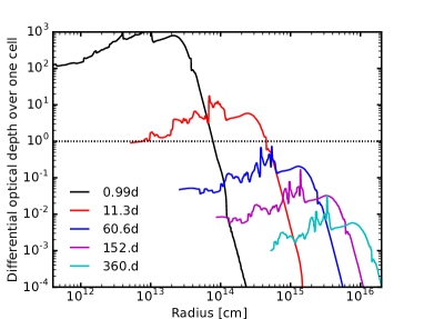
Figure 20: Differential optical depth of individual grid cells $\Delta\tau_{\gamma}$ of model B15 at different times for a randomly selected direction at $\theta=1.1$ and $\varphi=-2.0$. The dashed line indicates $\Delta\tau_{\gamma}=1$. Up to about $10\,$d the radiation is approximately trapped even within each cell of the numerical grid.

Figure 21: Radially integrated optical depth to the surface of the NiCoFe-rich ejecta $\tau_{\gamma}$ of model B15 at different times for a randomly selected direction at $\theta=1.1$ and $\varphi=-2.0$. The reference surface is defined by the outermost radii where the mass fraction of $X_{\mathrm{NiCoFe}}$ drops below $10^{-3}$. The dashed line indicates $\tau_{\gamma}=1$. Only later than $t\sim 150\,$d, the optical depth to the NiCoFe surface drops below $\tau_{\gamma}<1.0$ for most of the material.

In this Appendix, we test our implementation of the (local) energy deposition due to $\beta$ decay. As described in Section 2.2, we deposit only a fraction of the decay energy locally. This energy fraction depends on the interaction probability of the radiation with the ejecta, which is determined by the optical depth of the photons. The corresponding differential optical depth of individual numerical cells $\Delta\tau_{\gamma}$ is a measure for the radial optical depth of the local structures we can resolve within our simulations. $\Delta\tau_{\gamma}$ is plotted for model B15 and for a randomly chosen direction in Fig. 20. Up to about $t\gtrsim 10\,$d, this local optical depth is larger than one, meaning that until this time most energy is deposited locally inside the corresponding numerical cell. In Fig. 21, we show the radially integrated optical depth up to the NiCoFe surface, which is defined as the outermost radial location where the mass fraction of NiCoFe $X_{\mathrm{NiCoFe}}$ exceeds $10^{-3}$. Up to $t\sim 150\,$d, the optical depth $\tau_{\gamma}$ of most of the material is still significantly larger than $1$, and only after that time, the bulk of the material becomes transparent to the released $\gamma$ rays. Note that we always consider local deposition of the energy of the positron emitted during the ⁵⁶Co decay.

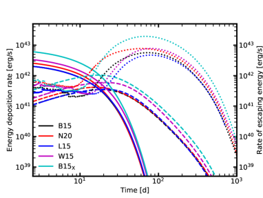
Figure 22: Volume integrated local $\beta$-decay energy deposition rates from ⁵⁶Ni (solid lines) and from ⁵⁶Co (dashed lines) compared to the rate of the energy which escapes from the NiCoFe-rich regions (dotted lines) for different models. After a few tens of days, more energy escapes from the NiCoFe-rich regions and around $t\sim 200\,$d the energy deposition rate inside the NiCoFe-rich volume drops to about one percent of the initial rate. Note that part of the escaping energy is deposited in the volume close to the NiCoFe-rich clumps.

In Fig. 22, we show the total energy deposition rates of the decaying ⁵⁶Ni (solid lines) and ⁵⁶Co (dashed lines) which is deposited locally for our different models. The dotted lines give the loss rate of the energy that depending on $\tau_{\gamma}^{\mathrm{mean}}$ is not deposited locally, but instead homogeneously or leaves the NiCoFe-rich region completely.

The total energy per second $dQ^{\text{tot}}/dt$ released due to the radioactive decay of ⁵⁶Ni and ⁵⁶Co is:

$$\frac{dQ_{\text{Ni}}^{\text{tot}}}{dt} = -\frac{\ln{2}}{\tau^{\text{Ni}}_{1/2}}N_{\text{Ni}}(t)Q_{\text{Ni}}\,$$ (19)

$$\frac{dQ_{\text{Co}}^{\text{tot}}}{dt} = -\frac{\ln{2}}{\tau^{\text{Co}}_{1/2}}N_{\text{Co}}(t)Q_{\text{Co}}\,,$$ (20)

where

$$N_{\text{Ni}}(t) = N_{\text{Ni}}^{0}\exp\left({-\frac{t\ln{2}}{\tau^{\text{Ni}}_{1/2}}}\right)\,,$$ (21)

$$N_{\text{Co}}(t) = N_{\text{Ni}}^{0}\frac{\tau^{\text{Co}}_{1/2}}{\tau^{\text{Ni}}_{1/2}-\tau^{\text{Co}}_{1/2}}\times$$ (22)

$$\left[\exp\left(-\frac{t\ln{2}}{\tau^{\text{Ni}}_{1/2}}\right)-\exp\left(-\frac{t\ln{2}}{\tau^{\text{Co}}_{1/2}}\right)\right]\,.$$

Initially, only a small fraction of the $\beta$-decay energy, which is emitted interior to the NiCoFe-surface, leaves the volume enclosed by this surface and most of the energy is deposited in the ejecta rich in NiCoFe. After about a few tens of days, ⁵⁶Co decay liberates more energy than ⁵⁶Ni decay, and the losses to the surroundings of the NiCoFe-rich ejecta exceed the locally deposited energy. At about $200\,$d the combined local deposition rate of ⁵⁶Ni and ⁵⁶Co is only one percent of the initial one.

Model	$E^{\mathrm{tot}}_{\mathrm{Ni}}=\int\Delta\epsilon_{\text{Ni}}dt$	$Q^{\mathrm{tot}}_{\mathrm{Ni}}=\int-\frac{dQ^{\text{tot}}_{\text{Ni}}}{dt}dt$	$E^{\mathrm{tot}}_{\mathrm{Co}}=\int\Delta\epsilon_{\text{Co}}dt$	$Q^{\mathrm{tot}}_{\mathrm{Co}}=\int-\frac{dQ^{\text{tot}}_{\text{Co}}}{dt}dt$	$(E^{\mathrm{tot}}_{\mathrm{Ni}}+E^{\mathrm{tot}}_{\mathrm{Co}})\times(Q^{\mathrm{tot}}_{\mathrm{Ni}}+Q^{\mathrm{tot}}_{\mathrm{Co}})^{-1}$
	[$10^{48}$erg]	[$10^{48}$erg]	[$10^{48}$erg]	[$10^{48}$erg]
B15	1.99	2.02	1.66	4.40	0.57
N20	2.47	2.59	1.83	5.63	0.52
L15	1.51	1.54	1.78	4.40	0.55
W15	3.31	3.30	3.10	7.21	0.61
B15${}_{\text{X}}$	5.95	6.07	4.71	13.2	0.55

Table 6: Integrated energies $E^{\mathrm{tot}}_{\mathrm{Ni}}$ (second column) and $E^{\mathrm{tot}}_{\mathrm{Co}}$ (fourth column) absorbed directly at the $\beta$-decay production sites. These values are compared to the theoretically expected total energy budget $Q^{\mathrm{tot}}_{\mathrm{Ni}}$ (third column) and $Q^{\mathrm{tot}}_{\mathrm{Co}}$ (fifth column) from integrating Eqs. 19 and 20, respectively. The last column gives the fraction of the total decay energy deposited directly at the production sites in the NiCoFeX-rich ejecta compared to the total energy budget of the respective decay.

As can be seen also in Fig.22, almost the entire decay energy from ⁵⁶Ni is deposited locally. We give the integrated energies deposited locally and produced during the different decays in Table 6 for the ⁵⁶Ni and ⁵⁶Co decays for all our models. Since the maximum of the ⁵⁶Co-decay occurs at times when the matter becomes transparent to $\gamma$ rays, only roughly $30-40\%$ of the energy of this decay is absorbed by the ejecta locally at the $\beta$-decay sites. This means in total, depending on the model $52-61\%$ of the total available energy budget of the ⁵⁶Ni-decay chain is transformed into the internal energy of the NiCoFe-rich ejecta.

References

- Abellán et al. (2017) Abellán F. J., et al., 2017, ApJ, 842, L24
- Alp et al. (2018a) Alp D., et al., 2018a, ApJ, 864, 174
- Alp et al. (2018b) Alp D., Larsson J., Fransson C., Gabler M., Wongwathanarat A., Janka H.-T., 2018b, ApJ, 864, 175
- Alp et al. (2019) Alp D., et al., 2019, ApJ, 882, 22
- Arcones et al. (2007) Arcones A., Janka H. T., Scheck L., 2007, A&A, 467, 1227
- Arnett et al. (1989) Arnett D., Fryxell B., Müller E., 1989, ApJ, 341, L63
- Basko (1994) Basko M., 1994, ApJ, 425, 264
- Benz et al. (1994) Benz W., Colgate S. A., Herant M., 1994, Physica D Nonlinear Phenomena, 77, 305
- Bethe (1990) Bethe H. A., 1990, Reviews of Modern Physics, 62, 801
- Blondin & Mezzacappa (2006) Blondin J. M., Mezzacappa A., 2006, ApJ, 642, 401
- Blondin et al. (2001) Blondin J. M., Borkowski K. J., Reynolds S. P., 2001, ApJ, 557, 782
- Blondin et al. (2003) Blondin J. M., Mezzacappa A., DeMarino C., 2003, ApJ, 584, 971
- Burrows et al. (1995) Burrows A., Hayes J., Fryxell B. A., 1995, ApJ, 450, 830
- Burrows et al. (2019) Burrows A., Radice D., Vartanyan D., 2019, MNRAS, 485, 3153
- Chevalier (1976) Chevalier R. A., 1976, ApJ, 207, 872
- Chevalier (2005) Chevalier R. A., 2005, ApJ, 619, 839
- Chevalier & Klein (1978) Chevalier R. A., Klein R. I., 1978, ApJ, 219, 994
- Childs et al. (2012) Childs H., et al., 2012, High Performance Visualization-Enabling Extreme-Scale Scientific Insight, pp 357–372
- Cigan et al. (2019) Cigan P., et al., 2019, ApJ, 886, 51
- Colella & Glaz (1985) Colella P., Glaz H. M., 1985, Journal of Computational Physics, 59, 264
- Colella & Woodward (1984) Colella P., Woodward P. R., 1984, Journal of Computational Physics, 54, 174
- Couch et al. (2009) Couch S. M., Wheeler J. C., Milosavljević M., 2009, ApJ, 696, 953
- Couch et al. (2011) Couch S. M., Pooley D., Wheeler J. C., Milosavljević M., 2011, ApJ, 727, 104
- DeLaney et al. (2010) DeLaney T., et al., 2010, ApJ, 725, 2038
- Einfeldt (1988) Einfeldt B., 1988, in Groenig H., ed., Shock Tubes and Waves. VCH, New York, pp 671–676
- Ellinger et al. (2012) Ellinger C. I., Young P. A., Fryer C. L., Rockefeller G., 2012, ApJ, 755, 160
- Ellinger et al. (2013) Ellinger C. I., Rockefeller G., Fryer C. L., Young P. A., Park S., 2013, preprint, (arXiv:1305.4137)
- Ertl et al. (2016a) Ertl T., Janka H.-T., Woosley S. E., Sukhbold T., Ugliano M., 2016a, ApJ, 818, 124
- Ertl et al. (2016b) Ertl T., Ugliano M., Janka H.-T., Marek A., Arcones A., 2016b, ApJ, 821, 69
- Fernández (2010) Fernández R., 2010, ApJ, 725, 1563
- Fesen (2001) Fesen R. A., 2001, ApJS, 133, 161
- Fesen & Gunderson (1996) Fesen R. A., Gunderson K. S., 1996, ApJ, 470, 967
- Foglizzo (2002) Foglizzo T., 2002, A&A, 392, 353
- Foglizzo et al. (2007) Foglizzo T., Galletti P., Scheck L., Janka H.-T., 2007, ApJ, 654, 1006
- Fryxell et al. (1991) Fryxell B., Arnett D., Müller E., 1991, ApJ, 367, 619
- Gawryszczak et al. (2010) Gawryszczak A., Guzman J., Plewa T., Kifonidis K., 2010, A&A, 521, A38
- Gessner & Janka (2018) Gessner A., Janka H.-T., 2018, ApJ, 865, 61
- Grefenstette et al. (2014) Grefenstette B. W., et al., 2014, Nature, 506, 339
- Grefenstette et al. (2017) Grefenstette B. W., et al., 2017, ApJ, 834, 19
- Hachisu et al. (1990) Hachisu I., Matsuda T., Nomoto K., Shigeyama T., 1990, ApJ, 358, L57
- Hachisu et al. (1992) Hachisu I., Matsuda T., Nomoto K., Shigeyama T., 1992, ApJ, 390, 230
- Hachisu et al. (1994) Hachisu I., Matsuda T., Nomoto K., Shigeyama T., 1994, A&AS, 104
- Hammer et al. (2010) Hammer N. J., Janka H.-T., Müller E., 2010, ApJ, 714, 1371
- Herant & Benz (1991) Herant M., Benz W., 1991, ApJ, 370, L81
- Herant & Benz (1992) Herant M., Benz W., 1992, ApJ, 387, 294
- Herant & Woosley (1994) Herant M., Woosley S. E., 1994, ApJ, 425, 814
- Hungerford et al. (2003) Hungerford A. L., Fryer C. L., Warren M. S., 2003, ApJ, 594, 390
- Hungerford et al. (2005) Hungerford A. L., Fryer C. L., Rockefeller G., 2005, ApJ, 635, 487
- Hunter (2007) Hunter J. D., 2007, Computing in Science and Engineering, 9, 90
- Isensee et al. (2010) Isensee K., Rudnick L., DeLaney T., Smith J. D., Rho J., Reach W. T., Kozasa T., Gomez H., 2010, ApJ, 725, 2059
- Iwamoto et al. (1997) Iwamoto K., Young T. R., Nakasato N., Shigeyama T., Nomoto K., Hachisu I., Saio H., 1997, ApJ, 477, 865
- Janka & Müller (1995) Janka H.-T., Müller E., 1995, ApJ, 448, L109
- Janka & Müller (1996) Janka H.-T., Müller E., 1996, A&A, 306, 167
- Janka et al. (2017) Janka H.-T., Gabler M., Wongwathanarat A., 2017, Proceedings of the International Astronomical Union, 12, 148–156
- Jerkstrand et al. (2018) Jerkstrand A., Ertl T., Janka H. T., Müller E., Sukhbold T., Woosley S. E., 2018, MNRAS, 475, 277
- Jerkstrand et al. (2020) Jerkstrand A., et al., 2020, MNRAS, 494, 2471
- Joggerst et al. (2009) Joggerst C. C., Woosley S. E., Heger A., 2009, ApJ, 693, 1780
- Joggerst et al. (2010a) Joggerst C. C., Almgren A., Bell J., Heger A., Whalen D., Woosley S. E., 2010a, ApJ, 709, 11
- Joggerst et al. (2010b) Joggerst C. C., Almgren A., Woosley S. E., 2010b, ApJ, 723, 353
- Jones et al. (01 ) Jones E., Oliphant T., Peterson P., et al., 2001–, SciPy: Open source scientific tools for Python, http://www.scipy.org/
- Junde et al. (2011) Junde H., Su H., Dong Y., 2011, Nuclear Data Sheets, 112, 1513
- Kageyama & Sato (2004) Kageyama A., Sato T., 2004, Geochemistry, Geophysics, Geosystems, 5, Q09005
- Kifonidis et al. (2003) Kifonidis K., Plewa T., Janka H.-T., Müller E., 2003, A&A, 408, 621
- Kifonidis et al. (2006) Kifonidis K., Plewa T., Scheck L., Janka H.-T., Müller E., 2006, A&A, 453, 661
- Larsson et al. (2016) Larsson J., et al., 2016, ApJ, 833, 147
- Larsson et al. (2019) Larsson J., et al., 2019, ApJ, 886, 147
- Lazendic et al. (2006) Lazendic J. S., Dewey D., Schulz N. S., Canizares C. R., 2006, ApJ, 651, 250
- Lentz et al. (2015) Lentz E. J., et al., 2015, ApJ, 807, L31
- Li et al. (1993) Li H., McCray R., Sunyaev R. A., 1993, ApJ, 419, 824
- Limongi et al. (2000) Limongi M., Straniero O., Chieffi A., 2000, ApJS, 129, 625
- Liou (1996) Liou M.-S., 1996, Journal of Computational Physics, 129, 364
- Lundqvist & Fransson (1991) Lundqvist P., Fransson C., 1991, ApJ, 380, 575
- Mao et al. (2015) Mao J., Ono M., Nagataki S., Hashimoto M.-A., Ito H., Matsumoto J., Dainotti M. G., Lee S.-H., 2015, ApJ, 808, 164
- Melson et al. (2015a) Melson T., Janka H.-T., Marek A., 2015a, ApJ, 801, L24
- Melson et al. (2015b) Melson T., Janka H.-T., Bollig R., Hanke F., Marek A., Müller B., 2015b, ApJ, 808, L42
- Melson et al. (2020) Melson T., Kresse D., Janka H.-T., 2020, ApJ, 891, 27
- Milisavljevic & Fesen (2013) Milisavljevic D., Fesen R. A., 2013, ApJ, 772, 134
- Milisavljevic & Fesen (2015) Milisavljevic D., Fesen R. A., 2015, Science, 347, 526
- Müller & Steinmetz (1995) Müller E., Steinmetz M., 1995, Computer Physics Communications, 89, 45
- Müller et al. (1991a) Müller E., Fryxell B., Arnett D., 1991a, in Danziger I. J., Kjaer K., eds, European Southern Observatory Conference and Workshop Proceedings Vol. 37, European Southern Observatory Conference and Workshop Proceedings. European Southern Observatory, Garching, p. 99
- Müller et al. (1991b) Müller E., Fryxell B., Arnett D., 1991b, A&A, 251, 505
- Müller et al. (2017) Müller B., Melson T., Heger A., Janka H.-T., 2017, MNRAS, 472, 491
- Müller et al. (2018) Müller B., Gay D. W., Heger A., Tauris T. M., Sim S. A., 2018, MNRAS, 479, 3675
- Nagataki et al. (1998) Nagataki S., Hashimoto M.-a., Sato K., Yamada S., Mochizuki Y. S., 1998, ApJ, 492, L45
- O’Connor & Couch (2018) O’Connor E. P., Couch S. M., 2018, ApJ, 865, 81
- Ohnishi et al. (2006) Ohnishi N., Kotake K., Yamada S., 2006, ApJ, 641, 1018
- Ono et al. (2013) Ono M., Nagataki S., Ito H., Lee S.-H., Mao J., Hashimoto M.-a., Tolstov A., 2013, ApJ, 773, 161
- Ono et al. (2020) Ono M., Nagataki S., Ferrand G., Takahashi K., Umeda H., Yoshida T., Orland o S., Miceli M., 2020, ApJ, 888, 111
- Orlando et al. (2016) Orlando S., Miceli M., Pumo M. L., Bocchino F., 2016, ApJ, 822, 22
- Orlando et al. (2019) Orlando S., et al., 2019, A&A, 622, A73
- Orlando et al. (2020a) Orlando S., et al., 2020a, A&A, 636, A22
- Orlando et al. (2020b) Orlando S., Wongwathanarat A., Janka H.-T., Miceli M., Ono M., Nagataki S., Bocchino F., Peres G., 2020b, arXiv e-prints, 2009, arXiv:2009.01789
- Ott et al. (2018) Ott C. D., Roberts L. F., da Silva Schneider A., Fedrow J. M., Haas R., Schnetter E., 2018, ApJ, 855, L3
- Perez & Granger (2007) Perez F., Granger B. E., 2007, Computing in Science and Engineering, 9, 21
- Plewa & Müller (1999) Plewa T., Müller E., 1999, A&A, 342, 179
- Quirk (1994) Quirk J. J., 1994, International Journal for Numerical Methods in Fluids, 18, 555
- Rest et al. (2011) Rest A., et al., 2011, ApJ, 732, 3
- Roberts et al. (2016) Roberts L. F., Ott C. D., Haas R., O’Connor E. P., Diener P., Schnetter E., 2016, ApJ, 831, 98
- Scheck et al. (2006) Scheck L., Kifonidis K., Janka H.-T., Müller E., 2006, A&A, 457, 963
- Scheck et al. (2008) Scheck L., Janka H.-T., Foglizzo T., Kifonidis K., 2008, A&A, 477, 931
- Shigeyama & Nomoto (1990) Shigeyama T., Nomoto K., 1990, ApJ, 360, 242
- Sinnott et al. (2013) Sinnott B., Welch D. L., Rest A., Sutherland P. G., Bergmann M., 2013, ApJ, 767, 45
- Stockinger et al. (2020) Stockinger G., et al., 2020, MNRAS, 496, 2039
- Strang (1968) Strang G., 1968, SIAM Journal on Numerical Analysis, 5, 506
- Summa et al. (2016) Summa A., Hanke F., Janka H.-T., Melson T., Marek A., Müller B., 2016, ApJ, 825, 6
- Swartz et al. (1995) Swartz D. A., Sutherland P. G., Harkness R. P., 1995, ApJ, 446, 766
- Takiwaki et al. (2014) Takiwaki T., Kotake K., Suwa Y., 2014, ApJ, 786, 83
- Utrobin et al. (2015) Utrobin V. P., Wongwathanarat A., Janka H.-T., Müller E., 2015, A&A, 581, A40
- Utrobin et al. (2017) Utrobin V. P., Wongwathanarat A., Janka H. T., Müller E., 2017, ApJ, 846, 37
- Utrobin et al. (2019) Utrobin V. P., Wongwathanarat A., Janka H. T., Müller E., Ertl T., Woosley S. E., 2019, A&A, 624, A116
- Vartanyan et al. (2018) Vartanyan D., Burrows A., Radice D., Skinner M. A., Dolence J., 2018, MNRAS, 477, 3091
- Vartanyan et al. (2019) Vartanyan D., Burrows A., Radice D., Skinner M. A., Dolence J., 2019, MNRAS, 482, 351
- Wang (2005) Wang C.-Y., 2005, ApJ, 626, 183
- Wongwathanarat et al. (2010) Wongwathanarat A., Janka H.-T., Müller E., 2010, ApJ, 725, L106
- Wongwathanarat et al. (2013) Wongwathanarat A., Janka H.-T., Müller E., 2013, A&A, 552, A126
- Wongwathanarat et al. (2015) Wongwathanarat A., Müller E., Janka H.-T., 2015, A&A, 577, A48
- Wongwathanarat et al. (2017) Wongwathanarat A., Janka H.-T., Müller E., Pllumbi E., Wanajo S., 2017, ApJ, 842, 13
- Woosley & Weaver (1995) Woosley S. E., Weaver T. A., 1995, ApJS, 101, 181
- Woosley et al. (1988) Woosley S. E., Pinto P. A., Ensman L., 1988, ApJ, 324, 466