Localised pair formation in bosonic flat-band Hubbard models

Abstract

Using a generalised version of Gershgorin’s circle theorem, rigorous boundaries on the energies of the lowest states of a broad class of line graphs above a critical filling are derived for hardcore bosonic systems. Also a lower boundary on the energy gap towards the next lowest states is established. Additionally, it is shown that the corresponding eigenstates are dominated by a subspace spanned by states containing a compactly localised pair and a lower boundary for the overlap is derived as well. Overall, this strongly suggests localised pair formationin the ground states of the broad class of line graphs and rigorously proves it for some of the graphs in it, including the inhomogeneous chequerboard chain as well as two novel examples of regular two dimensional graphs.

1 Introduction

1.1 Bosons in flat band systems

Due to the recent progress of both theoretical [1]-[8] and experimental [4, 7, 9, 10] nature, strongly correlated bosons on lattices have been gathering a lot of attention over the last few years. This has lead to improved understanding of several phenomena, including the Bose condensation and more recently the repulsive bosonic pair formation [11]-[14]. These papers investigate pair formation in very special classes of flat band systems.

A prototypical class of lattices with a flat band are line graphs with the kagome lattice as a prominent example [15]. Flat band models have been studied theoretically for more than 30 years to investigate phenomena in strongly correlated systems like ferrimagnetism [16], ferromagnetism [15, 17, 18, 19], or macroscopic magnetization jumps [20]. Since approximately ten years, they are studied also experimentally, mainly with the help of optical lattices, see e.g. [21]. And recently, flat bands are also studied in twisted bylayer graphene at some magic angles, see e.g. [22].

Flat bands are convenient to study strong correlation phenomena. Strong correlations occur if the interaction is large compared to the band width. In a flat band system, the latter vanishes. Therefore, an arbitrary small interaction is already sufficient to produce strong correlation effects. That explains the huge interest in flat band systems. On the other hand, all typical approximation methods that are based on perturbative approaches or mean field approaches will fail in flat bands due to the high degeneracy in the single particle spectrum. Therefore, many studies of flat band systems use mathematically rigorous methods.

Interestingly, the majority of rigorous results in flat band systems stems from fermionic systems or spin systems, whereas for bosonic systems less is known. One rigorous result for bosons in a flat band is the formation of a Wigner crystal at a critical density [23], which is valid for a large class of two-dimensional line graphs. Even below this critical density a full classification of all ground states is possible and one obtains a system with a residual entropy.

The above mentioned papers on bosonic pair formation in flat bands [11]-[14] focus on specific lattices and are to some degree based on numerical analysis or approximations without rigid error bounds. A rigorous analytical proof on the other hand, even in specific systems, has proven to be difficult. One important step towards this goal was achieved by Mielke [8], who proved pair formation for hard core bosons if one adds one particle to the system at the critical density of the Wigner crystal. But even there, the class of lattices is restricted to line graphs of graphs consisting of elementary cycles of length $4$ and with an additional condition on the hopping matrix elements. The hopping $t^{\prime}$ between the elementary cycles of length $4$ must be sufficiently smaller than the hopping $t$ on those cycles. We will provide a complete explanation of these hopping terms and of the construction of the lattices below.

1.2 Purpose of the present paper

This paper substantially generalises the class of graphs considered in [8] to include, among other things, two dimensional graphs with doubly periodic boundary conditions, and fills a gap in Mielke’s proofs by showing that the preconditions of his second theorem, which concerns the overlap of ground states with states containing a localised pair, are actually fulfilled under the conditions of the first theorem, thereby completing a first rigorous proof for the existence of localised pair formation in the ground state of certain systems. In addition to the chequerboard chain, where only the aforementioned gap was missing for such a proof, the systems with completely provable localised pair formation also include some novel two dimensional graphs, of which two are explicitly constructed.

Furthermore, several improvements on a qualitative as well as a quantitative level have been achieved. By introducing an asymmetrical norm and a simplified partitioning of the Fock space, we were able to increase the regime in which the theorem can be applied significantly, proved that both the energy of the lowest state and the gap to the next highest states are constant to first order in the secondary hopping parameter $t^{\prime}$ and were able to derive a concrete lower boundary for the overlap of the ground states with those of the uncoupled system (i.e. $t^{\prime}=0$.) While the complete proofs of localised pair formation make use of a specific local symmetry and some form of a global translational or rotational invariance, the main result of this paper, which already strongly suggests the existence of localised pair formation, does not require any kind of global symmetry in the class of graphs to which it applies.

1.3 The Hubbard model

The Hamiltonian of the bosonic Hubbard model is given by

$$H=\sum_{\{i,j\}\in E}t_{ij}b_{j}^{\dagger}b_{i}+\sum_{i\in V}U_{i}n_{i}(n_{i}-1).$$ (1)

Here $V$denotes the set of sites or vertices and edges of a Graph $G=(V,E)$ and $E$ is the set of edges. $b_{i}^{\dagger}(b_{i})$ denote the spinless bosonic creation (annihilation) operators on site $i$, $t_{ij}$ and $U_{i}$ are real parameters while $n_{i}=b_{i}^{\dagger}b_{i}$ is the particle number operator on site $i$.

Originally the model was independently proposed by Hubbard [27], Kanamori [28] and Gutzwiler [29] for fermionic systems and by Gersch and Knollman for bosonic systems [30]. While it strongly simplifies the interactions in a real solid, by reducing them to a hopping term with hopping strength $t_{ij}$ and an on site interaction $U_{i}$, it already correctly predicts plenty of effects in real solids including ferromagnetism [16, 15, 17, 18, 19] and superconductivity [32] in the fermionic, and superfluid-insulator transition [31] in the bosonic model. In many situations one will choose a translation invariant graph, homogeneous on site interaction and next-neighbour hopping (i.e. $U_{i}=U$ for all $i\in V$, $t_{ij}=t$ for $\{i,j\}\in E$ and $\{i,j\}\in E$ iff $|i-j|=1$). However, in the class of models under consideration in this paper we will need two different hoppings and will not require any kind of translational invariance as we will see later on. For more general background information we refer to overviews by Lieb [24], Tasaki [25] and Mielke [26], since we will focus our intention on the a certain subclass of Hubbard models: those on line graphs with a flat band.

1.4 Hubbard models on line graphs

There are multiple ways of constructing Hubbard models with single particle flat bands. One method is mentioned by Lieb [16]. As he points out, for any bipartite graph $G$ consisting of the two subgraphs $A$ and $B$ with $|B|=n|A|$ and $n\geq 2$ the hopping matrix $T$ with $T_{ij}=t$ for $\{i,j\}\in E$ and 0 otherwise has at most rank $2|A|$ and therefore at least $|V|-2|A|=|B|-|A|=(n-1)|A|$ zero eigenvalues. Consequently the system has $n-1$ flat bands in the centre of the spectrum. He was able to give the first proof of itinerant ferrimagnetism for these systems in case of a repulsive interaction (i.e. $U_{i}>0$ for all $i$.) Although here ferromagnetism only occurs in a weaker sense of the spin being an extensive quantity and is in fact not saturated, this example already shows why Hubbard models with flat bands are such interesting objects.

Of particular interest in the last years and focus of this work are Hubbard models with flat bands at the bottom of the spectrum. One class of graphs with such a low lying flat band is formed by decorated lattices, as they are treated for example by Tasaki [18], a second class are line graphs of bipartite and two-connected graphs [17].

As one can see from these examples, early research into graphs with flat bands focused heavily on fermionic systems. However, recent development has shown that bosons might be just as interesting to study on them, as we will discuss later on. Since line graphs are at the heart of the present work we will go over their construction. Our explanations are based on those presented in [8], which we generalise to also include toroidal graphs (i.e. graphs that can be drawn on a torus without having any edges crossing another one) and to weaken the condition on bipartition. We also refer to this work for greater details on some aspects of the construction.

We start with some finite, toroidal and two-connected graph $G=(V(G),E(G))$. It should be noted that the set of graphs that are both finite and planar is a subset of toroid graphs, therefore this work applies to them as well, while it also includes two dimensional graphs with doubly periodic boundary conditions (DPBC), which are not planar. Once again $V(G)$ and $E(G)$ denote the set of vertices and edges of $G$. The line graph of $G$ is now given by $L(G)=(V(L(G)),E(L(G)))$ with $V(L(G))=E(G)$ and $E(L(G))=\{\{e,e^{\prime}\}|e,e^{\prime}\in E(G),|e\cap e^{\prime}|=1\}$. For a more intuitive understanding, one can imagine the construction of the line graph from the original graph in the following way: We draw a vertex on each edge of the toroidal representation of $G$ and connect two vertices by an edge in $L(G)$ if and only if the edges they are drawn upon have a common vertex in the original graph. An illustration of the process for a simple square lattice can be found in the left two images of figure (1). On this line graph we can now define our Hamiltonian:

$$H=\sum_{\{e,e^{\prime}\}\in E(L(G))}\!\!t_{ee^{\prime}}b_{e^{\prime}}^{\dagger}b_{e}+\sum_{e\in V(L(G))}\!U_{e}n_{e}(n_{e}-1)$$ (2)

Furthermore, we will only consider the hard-core limit $U_{e}\to\infty$ for all $e$ such that at maximum one particle can be placed on each vertex in $L(G)$. Hence $H$ can be written as

$$H=P_{\leq 1}\!\!\sum_{\{e,e^{\prime}\}\in E(L(G))}\!\!t_{ee^{\prime}}b_{e^{\prime}}^{\dagger}b_{e}P_{\leq 1},$$ (3)

where $P_{\leq 1}$ denotes the projector on the subspace of the Fock space with at maximum one particle on each vertex.

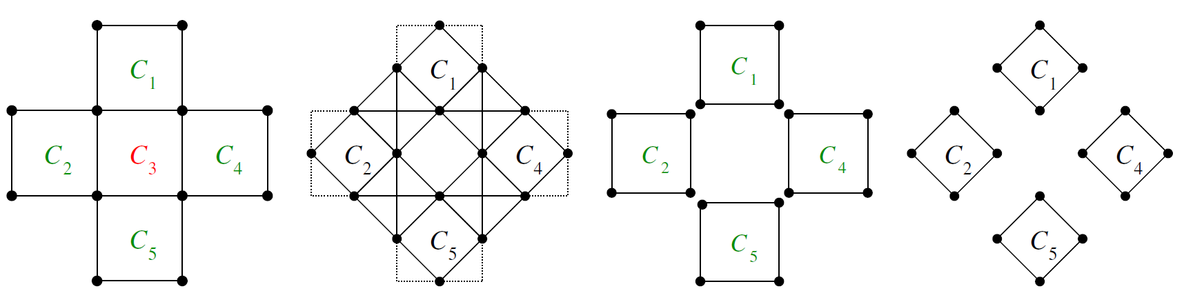
Figure 1: The left two images show a simple square lattice $G$ and its line graph $L(G)$. The members of $F_{1}(G)$, $C_{1}$, $C_{2}$, $C_{4}$, and $C_{5}$ are coloured in green and the right two images show the graph $G_{1}$ and its line graph $L(G_{1}).$ Figure taken from [8].

Before we can define the hopping strengths on the line graph, we first need to introduce some additional terms. The toroidal representation of the original graph $G$ decomposes the plane into faces and since a torus is a bounded object, all surfaces are bounded as well. We call the set of all null-homotopic faces $F(G)$ and by $C\in F(G)$ we denote both the surface itself and its boundary. Since $G$ is connected, there is at most one one-homotopic face. We call the elements of $F(G)$ elementary cycles (they are indeed cycles since $G$ is toroid.) Since the elementary cycles $C$ are subgraphs of $G$, we can define their set of vertices $V(C)$ and their set of edges $E(C)$. We now look at the colouring of the surfaces. We can colour two surfaces $C$ and $C^{\prime}$ with the same colour if they have no edge in common (i.e. $E(C)\cap E(C^{\prime})=\emptyset$).

Now let $F_{1}(G)\subset F(G)$ be the largest set of surfaces that can be coloured with the same colour and that all have even cycle length. Note that for a bipartite graph the second condition is trivially fulfilled for any subset of $F(G)$ since all cycles in bipartite graphs have even length. If there are multiple of these sets, we just choose one of them. By $E_{1}(G)$ we denote the set of edges, which form the boundaries in $F_{1}(G)$, $E_{1}(G)=\bigcup_{C\in F_{1}(G)}E(C)\subset E(G)$. Every edge in $E(G)$ belongs to a cycle in $F_{1}(G)$ if all faces that are not in $F_{1}(G)$, including the potential one-homotopic one, can be coloured by a single colour. Otherwise $E(G)\setminus E_{1}(G)$ is non-empty and we call its elements interstitials.

Additionally we define the graph $G_{1}$ which consists of all vertices and edges from cycles in $F_{1}(G)$ where we consider the vertices from different cycles to be distinct, even if they correspond to the same vertex in G. (See figure (1) for an illustration of the process.) Note that there is a one-to-one mapping between $E(G_{1})$ and $E_{1}(G)$ since every edge in $E_{1}(G)$ belongs to exactly one cycle in $F_{1}(G)$ (otherwise they could not all be coloured by the same colour) and therefore we write $E(G_{1})=E_{1}(G)$ while acknowledging the slight imprecision of the expression.

The same can however not be said about $V(G_{1})$ and $V_{1}(G)=\bigcup_{C\in F_{1}(G)}V(C)$ since one vertex in $V_{1}(G)$ can be counted for multiple times in $V(G_{1})$. Therefore, $V(L(G_{1}))=E(G_{1})=E_{1}(G)\subset E(G)=V(L(G))$ and two edges in $E(G_{1}),$ which are connected to a common vertex are also connected in $E(G),$ hence $E(L(G_{1}))\subset E(L(G).$ Consequently we conclude that $L(G_{1})$ is a subgraph of $L(G)$ an we can finally write down our hopping strengths:

$$t_{ee^{\prime}}=\begin{cases}t&\textrm{if }\{e,e^{\prime}\}\in E(L(G_{1}))\\ t^{\prime}&\textrm{if }\{e,e^{\prime}\}\in E(L(G))\setminus E(L(G_{1}))\end{cases}$$ (4)

This means we allow for hopping strength $t$ between the edges of elementary cycles and $t^{\prime}$ on all other edges of the line graph. Throughout this paper we choose $t>0$ and $t\geq t^{\prime}\geq 0$ and we will note additional restrictions whenever they become necessary. Furthermore it should be noted that since $G_{1}$ consists of isolated cycles, it is isomorphic to its line graph, meaning that any cycle $C\in F_{1}(G)$ corresponds to a cycle of the same length in $L(G)$ and every edge in $C\in F_{1}(G)$ corresponds to a vertex on the corresponding cycle in the line graph. This allows to rewrite our Hamiltonian:

$$H=tP_{\leq 1}\sum_{C\in F_{1}(G)}H_{C}P_{\leq 1}+t^{\prime}P_{\leq 1}\sum_{\langle C,C^{\prime}\rangle}H_{C,C^{\prime}}P_{\leq 1}+t^{\prime}H_{I}$$ (5)

Here $H_{C}$ describes the jumping on the elementary cycle $C$, $H_{C,C^{\prime}}$ the jumping between two neighbouring cycles $C$ and $C^{\prime}$ (i.e. $V(C)\cap V(C^{\prime})\neq\emptyset$) and $H_{I}$ the jumping to, from and between any interstitials.

1.5 Example: The chequerboard chain

There are many different graphs within this class, but to get a more concrete idea, we will have a closer look into one specific: the chequerboard chain. It is defined as the line graph of a chain of corner sharing squares and consists of a chain of cycles of length $|C|=4$, which are connected by complete graphs. It is depicted in figure (2). As it was also explained in [8], we can construct compactly localised one particle eigenstates $\psi_{C}$ with eigenvalue $-2t$ independently of $t^{\prime}$ on any cycle $C$ in the line graph by labeling an arbitrary vertex with the index $1$ and then we number them clockwise. Now we choose $\psi_{C}=\frac{1}{2}\!\left(\!b_{1}^{\dagger}(C)\!-\!b_{2}^{\dagger}(C)\!+\!b_{3}^{\dagger}(C)\!-\!b_{4}^{\dagger}(C)\!\right)|0\rangle$, where $b_{i}^{\dagger}(C)$ is a bosonic creation operator on site $i$ of cycle $C$; i.e. the absolute value is the same along the cycle while the sign alternates. It is easy to see that they are indeed eigenstates on $C$ with eigenvalue $-2t$ and the alternating signs ensure that the jumping terms to neighbouring cycles vanish. For $t^{\prime}<t$ these are unique ground states of the system. For $t^{\prime}=t$ they remain ground states, in case of periodic boundary conditions (PBC) they are no longer unique though. As the eigenstates on different cycles do not overlap, we can construct multi particle ground states from them, simply by putting at maximum one particle in the ground state of each cycle $C$. Again it turns out that these are the only ground states for $t^{\prime}<t$. This is possible until there are $N=|F_{1}(G)|$ particles in the system. We call this the critical density.

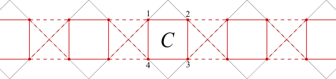
Figure 2: Illustration of the chequerboard chain: jumping on the cycles with hopping strength $t$ is indicated by a continuous read line, jumping between them with hopping strength $t^{\prime}$ by a dashed red line and for the graph of corner sharing graphs, whose line graph the chequerboardchain is, thin grey lines in the background are used.

1.6 Ground states at or below the critical density

In fact this result holds for the general class of graphs we are looking at. Mielke proved this for the class he was treating in [8] and the proof straightforwardly generalises to the larger class considered here. The precise statements are:

Proposition Let $G=(V(G),E(G))$ be a finite two-connected toroidal graph. Then for the Hubbard model on its line graph as defined in (5) the following holds: For $t>t^{\prime}\geq 0$ the ground state eigenvalue of the single particle Hamiltonian is $-2t$ and is $|F_{1}(G)|$-fold degenerate. For any $C\in F_{1}(G)$ a ground state is given by

$$\psi_{C}=\frac{1}{\sqrt{|C|}}\sum_{i=1}^{|C|}(-1)^{i+1}b_{i}^{\dagger}(C)|0\rangle$$ (6)

and its eigenvalue does not depend on $t^{\prime}$.

Here we have once again labeled an arbitrary edge of $C$ (corresponding to a vertex in the line graph) with $1$ and then numbered the others consecutively. Note that these are indeed eigenstates, since all cycles in $F_{1}(G)$ have even length and any hopping to other edges cancels out, since any edge in $G\setminus C$ that is connected to $C$ is connected to exactly two neighbouring edges in $C$. The proof for the larger class does not change compared to Mielke’s proof: The $\psi_{C}$ are still minima of the first term in the rewritten Hamiltonian and the only minima of the second term. Also it should be noted that these states remain ground states in the homogeneous case ($t=t^{\prime}$), although they are no longer unique in general. More precisely, if $G$ is planar, the ground states remain unique only if $F(G)\setminus F_{1}(G)$ contains no cycles of even length and if not, we need to additionally demand that no cycle that is a boundary of the potential one-homotopic face is of even length. Otherwise, additional linearly independent ground states can be placed on the line graphs of the corresponding cycles in the same manner as for the cycles in $F_{1}(G).$ This also explains, why for the homogeneous chequerboard chain the ground states remain unique for open boundary conditions, as its underlying graph is planar and $F(G)\setminus F_{1}(G)=\emptyset.$ On the other hand, for PBC the square chain surrounds either another face in $F(G)$ of even length if a planar representation is chosen or, if a non planar representation is chosen, there are two cycles of even length at the boundary of the one-homotopic face (for either of which the ground state on them can be added to the ones of the inhomogeneous case, to create a base of the ground states of the homogeneous system). For the multi particle ground states at or below the critical density the result is given by:

Proposition For $t>t^{\prime}>0$ and $N\leq|F_{1}(G)|$, the ground states of the Hubbard model on line graphs of finite two-connected toroidal graphs with $N$ hard core bosons are the same as the ones for $t^{\prime}=0$ and the ground state energy is $-2tN.$

The proof also generalises directly from Mielke’s proof to the broader class in question, since the eigenstates of the $t^{\prime}=0$ case remain eigenstates of the full Hamiltonian and are minima of the first term and the only minima of the second. Once again in the homogeneous case these states remain ground states but are no longer unique in general. For more information on the homogeneous case at or below the critical density, we refer to [23].

2 Hard core bosons above the critical density

As we have seen, we are able to characterize the ground states up to the critical density. The naturally occurring question is what happens if we add an additional particle beyond the critical density. To at least give a partial answer to that question, we need to establish some additional constraints on the class of graphs we are treating. First of all, we demand that there are no interstitials present on the line graph $L(G)$. This is equivalent to $\bigcup_{C\in F_{1}(G)}E(C)=E(G)$ and, as we have seen, can also be expressed as it being possible to colour the original graph $G$ (including the potential the potential one-homotopic face) where $F_{1}(G)$ contains all members of one colour. Additionally, we demand all cycles $C$ in $F_{1}(G)$ to be of length $4$. It is important to note that all other faces in $F(G)$ might have boundaries of arbitrary length.

Intuitively one can imagine the construction of an arbitrary graph in this class as follows: We start with a simple torus, which we colour in one colour, e.g. yellow, and then place a single quadrilateral on it, which we w.l.o.g. colour in blue. Now we continue to place additionalblue quadrilaterals on the torus which need to obey the following conditions: they need to be connected to the other quadrilaterals (i.e. if we number the quadrilaterals according to the order in which we place them on the torus and denote them by $C_{k}$, then for any $k$ there needs to be some $1\leq i<k$ such that $V(C_{k})\cap V(C_{i})\neq\emptyset$). It must not share an edge with any of the quadrilaterals (i.e. $E(C_{k})\cap E(C_{i})=\emptyset$ for $i\neq k$; this allows for quadrilaterals to have the same colour). Last they must not intersect with any of the previously placed quadrilaterals (i.e. leave the toroidal structure of the graph intact.) Now one repeats this process arbitrarily often and ends up with a graph that is toroidal, has only two colours and where the blue surfaces make up the elements of $F_{1}(G)$ and the potential remaining one-homotopic surface is coloured in yellow. Therefore, this graph has no interstitials, is two-connected (since removing any edge from a quadrilateral still allows for another path along the other three edges of the quadrilateral) and toroidal by construction.

Both the one dimensional chequerboard chain and its two dimensional analogue, the chequerboard lattice, are a member of this class for arbitrary boundary conditions. So are all other examples mentioned in figure 4 (for the regularly shaped ones once again regardless of boundary conditions) and figure 3 features a member of the class, which is not bipartite. Other interesting cases like the kagome lattice are however not, as its cycles have length six and three colours are necessary to colour its underlying graph, the honeycomb lattice. The limitation to cycles of length $4$ could be avoided without much theoretical difficulty. However, the results become generally worse with longer cycles, as it is energetically less expensive to put multiple particles into one cycle and mixed cycle lengths would require additional treatment. The reason we are excluding the existence of interstitials is that they allow for additional possibilities for the additional particle to spread to.

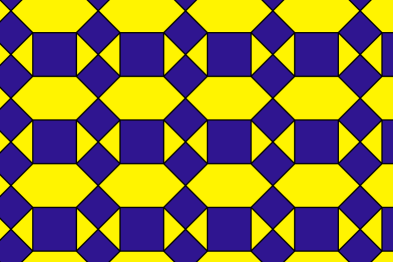
Figure 3: Example of a non-bipartite graph $G$ within the class of graphs, to which the main result applies. It includes cycles of length 3 (the yellow triangles), but since they do not appear among the surfaces of $F_{1}(G)$ (coloured in blue), we can still construct localised eigenstates as described in section 1.6 on the graph.

Under these conditions our initial question (What would happen if there is an additional particle placed on the line graph?) has an obvious answer for $t^{\prime}=0$: The additional particle can simply be put on any cycle $C\in F_{1}(G)$ to form the two particle ground state (which has energy $-2\sqrt{2}t$, see table 1 for its precise form) and still have one particle each in the single particle ground state on each other cycle, we call these ground states $\varphi_{C}$ and they span any ground state for $t^{\prime}=0.$ We denote this subspace by $\Omega_{0}$ and the projector onto it by $P_{0}$. Since the two particle one cycle ground state is no longer an eigenstate for $t^{\prime}\neq 0,$ the result for the uncoupled system can no longer be as easily generalised to the full Hamiltonian. We were however able to derive rigorous boundaries for the energy of the lowest states, to show how they remain separated from the rest of the spectrum and how they are dominated by the ground states of the uncoupled system.

Before we get to it, we however need to quote one more result on the chequerboard chain by Drescher and Mielke, which we will also extend to some additional graphs, to understand the full importance of our result for these specific graphs.

2.1 Degeneracy of ground states of graphs possessing a local reflection symmetry

We look at the chequerboard chain with PBC. Using a symmetry argument, Drescher and Mielke were able to show the following result, which we slightly rephrase to cater towards the needs of this work [14]:

Proposition (Drescher, Mielke, 2017) If for some ground state $\varphi_{1}$ of $H$ on the chequerboard chain with PBC, there is an overlap with the ground states of the uncoupled system (i.e. $\|P_{0}\varphi\|_{2}\neq 0$), then the ground states are at least $|F_{1}(G)|$ fold degenerated.

This can be proved using a symmetry property of the chequerboard chain: Its Hamiltonian remains invariant under exchanges of the lower vertices with their upper counterparts (i.e. in figure 2 to interchange vertex 1 with 4 and 2 with 3, respectively, or, equivalently, to exchange the upper and lower edges of the square in the original graph) for any cycle $C$ and we call the operator that performs this operation $S_{C}$. Therefore, it is possible to find a common base of eigenstates of $H$ and all of the $S_{C}$ (as they also commute with one another.) Since the base states of $\Omega_{0},$ $\varphi_{C^{\prime}}$ have eigenvalue $2\delta_{C,C^{\prime}}-1$ under $S_{C},$ there is a unique signature for all base states. Now we look at a ground state $\varphi_{1}$ of H with $\|P_{0}\varphi_{1}\|_{2}\neq 0$ which is also an eigenstates of all $S_{C}.$ Therefore, its signature needs to be identical to one of the base states of $\Omega_{0}$. Additionally, the Hamiltonian is invariant under shifting the state by one face to the right due to the PBC. Hence, the resulting state $\varphi_{2}$ must also be a ground state but since its signature differs from the one of $\varphi_{1}$ they cannot be identical. This argument can be repeated to create $|F_{1}(G)|$ ground states $\varphi_{k}$ with unique signatures, which therefore are linearly independent, which proves the proposition. Moreover the $\varphi_{k}$ only overlap with a single base state of $\Omega_{0}$, the one they share the signature with. Hence they obey $P_{0}\varphi_{k}=r\varphi_{C}$, for some $C\in F_{1}(G)$ and $0<|r|\leq 1$, i.e. their projector into into $\Omega_{0}$ has a compactly localised pair.

We now look at the lattice of intertwined rhombi chains (abbreviated LIR (4,1), here 4 stands for the maximum number of rhombi that share a single vertex and 1 for the number rhombi between two such vertices) with DPBC as depicted in figure 4(a)). Since the rhombi share only corners but not edges, they can indeed be coloured by one colour and they form the set $F_{1}(G).$ One immediately notices that its line graph does possess the same local reflection symmetry, since for all rhombi the mirroring on the longer diagonal leaves the Hamiltonian of the line graph invariant and we can again find a common base of eigenstates of $H$ and all $S_{C}.$ Any ground state of $H$ in this basis can overlap with at maximum one base state of $\Omega_{0}.$ Now we assume such an overlapping ground state, $\varphi_{1},$ does indeed exist and $\varphi_{C}$ is the state it overlaps with. Then we can again use the translational invariance due to the DPBC to find additional ground states which overlap with different base states of $\Omega_{0}.$ This is possible for all $\varphi_{C}^{\prime}$ as long as $C$ and $C^{\prime}$ share the same spatial orientation (i.e. are either both members of a horizontal or both members of a vertical chain.) Now we additionally demand that the lattice has the same length in both directions and call this the symmetric case. The Hamiltonian is then also invariant under a global rotation by $\frac{\pi}{2}$ around an arbitrary vertex of $G$ which connects multiple rhombi. This maps $C$ onto a rhombus of different orientation and therefore transforms $\varphi_{k}$ onto a ground state overlapping with a state in $\Omega_{0}$ with two particles on that rhombus. Repeating the translations we can find a ground state of $H$ which exactly overlaps with $\varphi_{\bar{C}}$ for every $\bar{C}\in F_{1}(G).$

Similarly one can work out the ground state degeneracy under this condition for the line graph of the thinned out lattice of intertwined rhombi (abbreviated LIR (3,2), use of the numbers in accordance to the (4,1) case.) It is depicted in figure 4(b)). Starting from one ground state with a given signature we can use the translational invariance to find linearly independent ground states with signature $+1$ on every rhombus in the lattice, given it has the same position in the ”rotor” the graph is build from (marked in blue in fig 4(b)).) The rhombi enclose regular hexagons which can be thought of as a honeycomb lattice, if we consider the rhombi to be their edges. If all chains of hexagons have the same length, we call this again the symmetric case. In this case, the Hamiltonian is invariant under rotations by $\frac{\pi}{3}$ around the centre of any ”hexagon” which allows us to find find ground states with signature $+1$ on every rhombus of the ”basic rotor” and in combination with the translational invariance, we achieve the same result as for the chequerboard chain:

Proposition If the line graphs of the symmetric LIR (4,1) with DPBC or of the symmetric LIR (3,2) with DPBC possess a ground state $\varphi_{1}$ of $H$ that has an overlap with the ground states of the uncoupled system (i.e. $\|P_{0}\varphi\|_{2}\neq 0$),the ground states are at least $|F_{1}(G)|$ fold degenerated.

(a) The LIR (4,1)

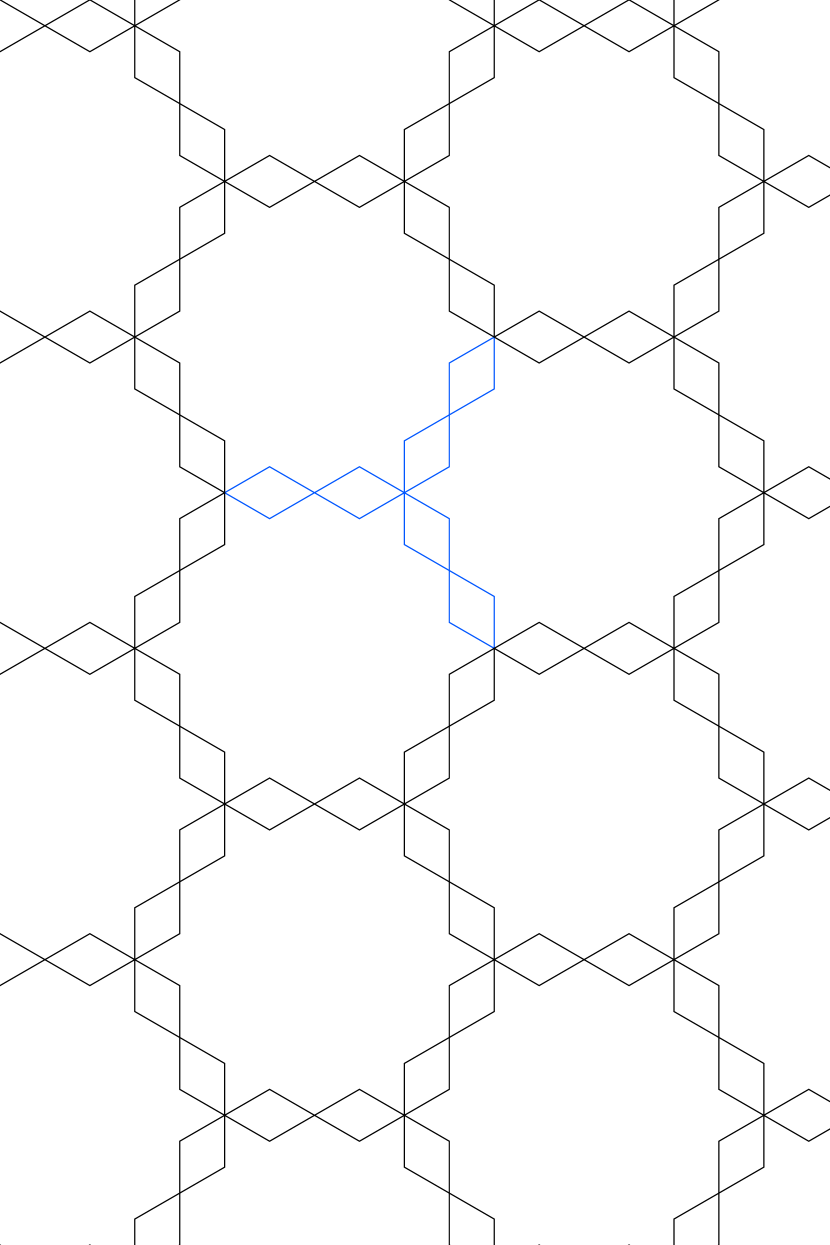
(b) The LIR(3,2)

(c) The 12 rhombi star

Figure 4: Several toroidal graphs obeying a local reflection symmetry.

Remarks: Several similar regular two dimensional lattices obeying this local symmetry can be found. We decided to present these two specifically because the (4,1) version seems like the most intuitive one, while in the (3,2) case every rhombus only neighbours three others, which is the minimal possible number for a regular two dimensional structure which proves to be beneficial for the main result.

Given a sufficiently small acute angle, one can of course attach arbitrarily many rhombi to a central vertex and we call this the $n$ rhombi star. Essentially the LIR are build up from such stars for $n=4$ and $n=3$, respectively. For $n=12$ it is depicted in figure 4(c)). Since it obeys the local reflection symmetry and is invariant under global rotations by $\frac{2\pi}{n}$ around its centre, an analogue proof for the degeneracy of its ground state energy is possible. However,since the number of other next neighbours is proportional to the number of rhombi within the graph, the main result very quickly gets extremely bad even for a moderate number of rhombi (and therefore allowed particles in the systems). Hence, we consider the (isolated) star with an arbitrary $n$ to be more of an academic curiosity, than a physically relevant system (at least in the context of localised pair formation).

While the energetic degeneracy depends on some form of a global symmetry,the possibility to find ground states that overlap with at maximum one base state of $\Omega_{0}$ only relies on the existence of the local reflection symmetry for all $C.$ Therefore, it also holds for all other graphs in our class obeying this symmetry. Examples of graphs obeying the local symmetry but without any kind of global rotational or translational invariance are treelike structures such as the one described in chapter 5 of [8].

2.2 Main result

Under the conditions set out at the beginning of this chapter we now show the following rigorous bounds for the energy of the lowest energy states of $H$ as well as for the gap to the next lowest states up to a certain $t^{\prime}_{\sup}$ and show that they are dominated by states in $\Omega_{0}.$

Theorem Let $G$ be a two-connected toroidal graph with $\bigcup_{C\in F_{1}(G)}E(C)=E(G)$ and $|C|=4$ for all $C\in F_{1}(G)$. Then the following holds for $t^{\prime}<t^{\prime}_{\sup}$:

1. The Hamiltonian

   $$H=tP_{\leq 1}\sum_{C\in F_{1}(G)}H_{C}P_{\leq 1}+t^{\prime}P_{\leq 1}\sum_{C\neq C^{\prime}\in F_{1}(G)}H_{C,C^{\prime}}P_{\leq 1}$$ (7)

   with $N=|F_{1}(G)|+1$ hard core bosons on $L(G)$ has exactly $|F_{1}(G)|$ linearly independent eigenstates with energies $E_{k}$ in the lowest interval, sufficing

   $$-\left(2N-e_{5}\right)t-b\sqrt{c(G)}\eta_{+}(t^{\prime})t^{\prime}\leq E_{k}\leq-\left(2N-e_{5}\right)t.$$ (8)

2. The energy gap $\Delta$ between these lowest and the upper states satisfies

   $$\Delta\geq e_{5}t-\left(a\frac{t^{\prime}}{t}c^{2}(G)+b\eta_{-}(t^{\prime})\sqrt{c(G)}\right)t^{\prime}.$$ (9)

   .

3. The corresponding eigenstates $\varphi_{k}$ satisfy

   $$\|P_{0}\varphi_{k}\|_{2}\geq\left(1+\eta_{-}^{2}(t^{\prime})\right)^{-\frac{1}{2}}\|\varphi_{k}\|_{2}.$$ (10)

Where

$$\begin{split}t^{\prime}_{\sup}&=\left(\sqrt{\frac{b^{2}}{a^{2}c(G)}+\frac{e_{5}}{a}}-\frac{b}{a\sqrt{c(G)}}\right)\frac{t}{c(G)}\\ &=0.6120\left(\sqrt{\frac{0.08478}{c(G)}+1}-\frac{0.2912}{\sqrt{c(G)}}\right)\frac{t}{c(G)},\end{split}$$ (11)

$$\begin{split}\eta_{\pm}(t^{\prime})=&\dfrac{2b\sqrt{c(G)}}{\left(e_{5}-a\tilde{t}^{2}c^{2}(G)\right)+\sqrt{\left(e_{5}-a\tilde{t}^{2}c^{2}(G)\right)^{2}\pm 4b^{2}\tilde{t}^{2}c(G)}}\tilde{t}\\ =&\dfrac{b\sqrt{c(G)}}{e_{5}}\tilde{t}+\mathcal{O}\left(\tilde{t}^{3}\right),\end{split}$$ (12)

$\tilde{t}=\frac{t^{\prime}}{t}.$ $e_{5}$, $a$ and $b$ are numerical constants:

$$e_{5} =2\left(2-\sqrt{2}\right)=1.1714$$

$$a =\frac{1425+974\sqrt{2})}{896}=3.1277$$

$$b =\sqrt{\frac{3}{4}\left(\sqrt{2}-1\right)}=0.5574$$

$P_{0}$ denotes the projector into the $N$ particle ground states of

$$H_{F_{1}(G)}=tP_{\leq 1}\sum_{C\in F_{1}(G)}H_{C}P_{\leq 1}$$ (13)

and $\|\psi\|_{2}=\left(\sum_{i=1}^{n}|\psi_{i}|^{2}\right)^{\frac{1}{2}}$ the standard euclidean norm on the $N$ particle Fock space w.r.t. the base of eigenstates of $H_{F_{1}(G)}$.

Proof: For our proof we will make use of a generalised version of of Gershgorin’s circle theorem by Feingold and Varga [33]. They showed the following: Let $A$ be a square matrix which is acting on a space $\Omega$ and is partitioned in the following manner:

$$A=\begin{pmatrix}A_{11}&A_{12}&\dots&A_{1m}\\ A_{21}&A_{22}&\dots&A_{2m}\\ \vdots&\vdots&\ddots&\vdots\\ A_{m1}&A_{m2}&\dots&A_{mm}\end{pmatrix}$$ (14)

Where the $A_{ii}$ are square matrices acting on $n_{i}$ dimensional subspaces $\Omega_{i}$ of $\Omega$, therefore $\sum_{i=1}^{m}n_{i}=n=:\dim(\Omega)$ and the $A_{ij}$ are $n_{i}\times n_{j}$ matrices. Then for every eigenvalue $\lambda$ of $A$ there is at least one $i$, $1\leq i\leq m$ such that:

$$\left(\left\|\left(A_{ii}-\lambda I_{i}\right)^{-1}\right\|\right)^{-1}\leq\sum_{k=1,k\neq i}^{m}\left\|A_{ik}\right\|$$ (15)

Here $I_{i}$ denotes the unit matrix on $\Omega_{i}$ and the matrix norms are the ones derived by the corresponding vector norms:

$$\left\|A_{ij}\right\|=\max_{\begin{subarray}{c}x\in\Omega_{j}\\ \|x\|_{\Omega_{j}}=1\end{subarray}}\left\|A_{ij}x\right\|_{\Omega_{i}}$$ (16)

It is important to note that the vector norms on the $\Omega_{i}$ can be chosen arbitrarily and independent of each other. Also, since

$$\left(\left\|B^{-1}\right\|\right)^{-1}=\min_{\|x\|=1}\left\|Bx\right\|$$ (17)

for any invertible matrix $B$, it is the natural continuation to define $\left(\left\|B^{-1}\right\|\right)^{-1}=0$ for singular$B$.

Once again let $\Omega_{0}$ be the space spanned by the ground states $\varphi_{C}$ of $H_{F_{1}(G)}$, $\Omega_{1}$ its orthogonal subspace and $P_{1}=1-P_{0}$ the corresponding projector. Then we can write H as

$$H=\begin{pmatrix}H_{0}&H_{01}\\ H_{10}&H_{1}\end{pmatrix}=\begin{pmatrix}P_{0}HP_{0}&P_{0}HP_{1}\\ P_{1}HP_{0}&P_{1}HP_{1}\end{pmatrix}.$$ (18)

Furthermore we choose our norms as $\|\cdot\|_{\Omega_{0}}=\eta\|\cdot\|_{2}$ and $\|\cdot\|_{\Omega_{1}}=\|\cdot\|_{2}$ where $\|\cdot\|_{2}$ is the euclidean norm on $\Omega_{i}$, $i=0,1$ and $\eta$ a positive real number, which we will specify later on.

Now our goal is to show that

$$\begin{split}\sup\Lambda_{0}:=&\sup\Big{\{}\lambda\in\mathbb{R}\Big{|}\left(\left\|\left(H_{0}-\lambda I_{0}\right)^{-1}\right\|\right)^{-1}\leq\left\|H_{01}\right\|\Big{\}}\\ <&\inf\Big{\{}\lambda\in\mathbb{R}\Big{|}\left(\left\|\left(H_{1}-\lambda I_{1}\right)^{-1}\right\|\right)^{-1}\leq\left\|H_{10}\right\|\Big{\}}=:\inf\Lambda_{1}\end{split}$$ (19)

for all $t^{\prime}<t^{\prime}_{\sup}$ and an appropriate choice of $\eta$. Since we know that for $t^{\prime}=0$ there are exactly $|F_{1}(G)|$ eigenvalues of $H$ in $\Lambda_{0}$ and the eigenvalues vary continuouslyin $t^{\prime}$, this number cannot change as long as the two sets are disjoint. Therefore, we will have proven the separation of the lowest eigenvalues from the others and will also be able to establish an upper boundary for their values.

We start by looking at $\Lambda_{0}$. Since $H_{0}=\left(-2(N-2)-2\sqrt{2}\right)tI_{0}$ we have

$$\left(\left\|\left(H_{0}-\lambda I_{0}\right)^{-1}\right\|\right)^{-1}=\left|\left(-2(N-2)-2\sqrt{2}\right)t-\lambda\right|.$$ (20)

Also

$$\begin{split}\|H_{01}\|&=\max_{\begin{subarray}{c}\psi\in\Omega_{1}\\ \|\psi\|_{\Omega_{1}}=1\end{subarray}}\|H_{01}\psi\|_{\Omega_{0}}\\ &=\eta\sqrt{\rho\left(H_{01}^{\dagger}H_{01}\right)}\\ &=\eta\sqrt{\rho\left(H_{01}H_{01}^{\dagger}\right)}\\ &=\eta\sqrt{\rho\left(H_{01}H_{10}\right)},\end{split}$$ (21)

where $\rho(\cdot)$ is the spectral radius of a matrix. The third equality holds because the spectral radius is invariant under Hermitian transposition and the last one due to $H$ being Hermitian. One finds the eigenvectors of $H_{01}H_{10}$ to be the same as the eigenvectors of $H_{0}$ and their eigenvalues to be $\lambda_{k}=(\frac{3}{4}(\sqrt{2}-1))c(C_{k})t^{\prime 2}=:b^{2}c(C_{k})t^{\prime 2}$. Where $C_{k}$ is the cycle occupied by two particles in the $k$th eigenstate of $H_{0}$. Hence we can conclude

$$\|H_{01}\|=\eta b\sqrt{c(G)}t^{\prime}.$$ (22)

Combining (20) and (21) we get

$$\Lambda_{0}=\Big{\{}\lambda\in\mathbb{R}\Big{|}\;\left|\left(-2(N-2)-2\sqrt{2}\right)t-\lambda\right|\leq\eta b\sqrt{c(G)}t^{\prime}\Big{\}}$$ (23)

and subsequently

$$\sup\Lambda_{0}=\left(-2(N-2)-2\sqrt{2}\right)t+\eta b\sqrt{c(G)}t^{\prime}.$$ (24)

For $\Lambda_{1}$ the calculation is not as straight forward. $H_{1}$ is non diagonal and therefore we need to look at $\big{(}\big{\|}\left(H_{1}-\lambda I_{1}\right)^{-1}\big{\|}\big{)}^{-1}$ more carefully. Let $S$ be a diagonal Matrix with $S_{kk}>0$ for all $k$. Then $S$ is non-singular and we can apply proposition 1.1 of [34] to achieve the following lower bound

$$\begin{split}&\left(\left\|\left(H_{1}-\lambda I_{1}\right)^{-1}\right\|\right)^{-1}\\ \geq&\left(\left\|\left(S\left(H_{1}-\lambda I_{1}\right)S^{-1}\right)^{-1}\right\|_{1}\left\|\left(S^{-1}\left(H_{1}-\lambda I_{1}\right)S\right)^{-1}\right\|_{\infty}\right)^{-\frac{1}{2}}\\ =&\left(\left\|\left(S\left(H_{1}-\lambda I_{1}\right)S^{-1}\right)^{-1}\right\|_{1}\right)^{-1}\\ =&\min_{\|\psi\|_{1}=1}\left\|S\left(H_{1}-\lambda I_{1}\right)S^{-1}\psi\right\|_{1}\\ =&\min_{\|\psi\|_{1}=1}\sum_{i=1}^{n_{1}}\Big{|}\left(S(H_{1}-\lambda I_{1})S^{-1}\right)_{ii}\psi_{i}+\sum_{j\neq i}\left(SH_{1}S^{-1}\right)_{ij}\psi_{j}\Big{|}\\ =&\min_{\|\psi\|_{1}=1}\sum_{i=1}^{n_{1}}\Big{|}(H_{1;ii}-\lambda)\psi_{i}+\sum_{j\neq i}S_{ii}H_{1;ij}S_{jj}^{-1}\psi_{j}\Big{|}\\ \geq&\min_{\|\psi\|_{1}=1}\sum_{i=1}^{n_{1}}\Big{(}|H_{1;ii}-\lambda||\psi_{i}|-\sum_{j\neq i}|S_{ii}H_{1;ij}S_{jj}^{-1}||\psi_{j}|\Big{)}\\ =&\min_{\|\psi\|_{1}=1}\sum_{i,j=1}^{n_{1}}|S_{ii}H_{1;ij}S_{jj}^{-1}-\lambda\delta_{ij}||\psi_{j}|(2\delta_{ij}-1)\\ =&\min_{\|\psi\|_{1}=1}\sum_{j=1}^{n_{1}}|\psi_{j}|\Big{(}|H_{1;jj}-\lambda|-\sum_{i\neq j}|S_{ii}H_{1;ij}S_{jj}^{-1}|\Big{)}\\ =&\min_{1\leq k\leq n_{1}}\Big{(}|H_{1;kk}-\lambda|-\sum_{i\neq k}|S_{ii}H_{1;ik}S_{kk}^{-1}|\Big{)}\min_{\|\psi\|_{1}=1}\sum_{j=1}^{n_{1}}|\psi_{j}|\end{split}$$ (25)

$$= \min_{1\leq k\leq n_{1}}\Big{(}|H_{1;kk}-\lambda|-\sum_{i\neq k}|S_{ii}H_{1;ik}S_{kk}^{-1}|\Big{)}.$$ (26)

We are interested in $\inf\Lambda_{1}$ and $\lambda=\left(-2(N-4)-4\sqrt{2}\right)t$ fulfils

$$\min_{1\leq k\leq n_{1}}\Big{(}|H_{1;kk}-\lambda|-\sum_{i\neq k}|S_{ii}H_{1;ik}S_{kk}^{-1}|\Big{)}\leq\left\|H_{10}\right\|$$ (27)

trivially for all $t^{\prime},$ as it is the lowest non ground state eigenvalue of $H_{F_{1}(G)}$. Therefore, we now assume $\lambda\leq\left(-2(N-4)-4\sqrt{2}\right)t$ and note $\lambda\leq H_{1;kk}$ for all $1\leq k\leq n_{1}$. Consequently we can drop the absolute value in the first term without changing its value. Our next goal is to rewrite the argument of (26) as a constant independent of $k$ plus a sum over the connections between neighbouring cycles. To achieve this we introduce $e_{i}$, the difference between the energy $\frac{E_{i}}{t}$ of the $i$th one cycle eigenstate (normalised by $t$) and the again normalised energy of distributing all $N_{i}$ particles in the state in one particle ground states;

$$e_{i}=\frac{E_{i}}{t}+2N_{i}.$$ (28)

If the cycle $C$ is occupied by the $i$th one cycle eigenstate in $\chi_{k}$, the $k$th base state of $H_{1},$ we then write $N_{k}(C)=N_{i}$, $E_{k}(C)=E_{i}$ and $e_{k}(C)=e_{i}$, which allows us to rewrite $H_{1;kk}$ as

$$\begin{split}H_{1;kk}&=\sum_{C}E_{k}(C)\\ &=\sum_{C}\left(e_{k}(C)-2N_{k}(C)\right)t\\ &=-2Nt+\sum_{C}e_{k}(c)t,\end{split}$$ (29)

since $\sum_{C}N_{k}(C)=N$ for all $k$ by definition. The values of all $e_{i}$ are given in table 1.

$i$	$\beta_{i}^{\dagger}$	$s_{i}$	$e_{i}$	$\mu_{i}$	$\nu_{i}$
0	$\mathbb{1}$	1	0	0	$\frac{1}{\alpha}\!\left(\!\sqrt{2}\!+\!1\!\right)$
1	$\frac{1}{2}\!\left(\!b_{1}^{\dagger}\!-\!b_{2}^{\dagger}\!+\!b_{3}^{\dagger}\!-\!b_{4}^{\dagger}\!\right)$	$\alpha$	0	0	$\frac{1}{\alpha}\!\sqrt{2}$
2	$\frac{1}{\sqrt{2}}\!\left(\!b_{1}^{\dagger}\!-\!b_{3}^{\dagger}\!\right)$	$\alpha$	$2$	$\frac{\alpha}{\sqrt{2}}$	$\frac{\alpha}{2\sqrt{2}}\!+\!\frac{3}{2\alpha}\!\left(\!1\!+\!\frac{1}{\sqrt{2}}\!\right)$
3	$\frac{1}{\sqrt{2}}\!\left(\!b_{2}^{\dagger}\!-\!b_{4}^{\dagger}\!\right)$	$\alpha$	$2$	$\frac{\alpha}{\sqrt{2}}$	$\frac{\alpha}{2\sqrt{2}}\!+\!\frac{3}{2\alpha}\!\left(\!1\!+\!\frac{1}{\sqrt{2}}\!\right)$
4	$\frac{1}{2}\!\left(\!b_{1}^{\dagger}\!+\!b_{2}^{\dagger}\!+\!b_{3}^{\dagger}\!+\!b_{4}^{\dagger}\!\right)$	$\alpha$	4	$\alpha$	$\alpha\!\frac{\sqrt{2}-1}{2}\!+\!\frac{1}{\alpha}\!\left(\!\sqrt{2}\!+\!\frac{1}{2}\!\right)$
5	$\frac{1}{2}\left(\!b_{1}^{\dagger}b_{3}^{\dagger}\!+\!b_{2}^{\dagger}b_{4}^{\dagger}\!\right)$	1	$4\!-\!2\sqrt{2}$	$\frac{1}{\alpha}\!\left(\!\sqrt{2}\!-\!1\!\right)$	$\frac{1}{d\alpha}\!\left(\!\sqrt{2}\!-\!1\!\right)$
	$-\frac{1}{2\sqrt{2}}\!\left(\!b_{1}^{\dagger}b_{2}^{\dagger}\!+\!b_{2}^{\dagger}b_{3}^{\dagger}\!+\!b_{3}^{\dagger}b_{4}^{\dagger}\!+\!b_{1}^{\dagger}b_{4}^{\dagger}\!\right)$
6	$\frac{1}{\sqrt{2}}\left(\!b_{1}^{\dagger}b_{3}^{\dagger}\!-\!b_{2}^{\dagger}b_{4}^{\dagger}\!\right)$	$\alpha^{2}$	4	$\alpha\!\left(\!1\!+\!\frac{1}{\sqrt{2}}\!\right)$	$\frac{\alpha}{d}\!\left(\!1\!+\!\frac{1}{\sqrt{2}}\!\right)$
7	$\frac{1}{\sqrt{2}}\left(\!b_{1}^{\dagger}b_{2}^{\dagger}\!-\!b_{3}^{\dagger}b_{4}^{\dagger}\!\right)$	$\alpha^{2}$	4	$\alpha\!\left(\!1\!+\!\frac{1}{\sqrt{2}}\!\right)$	$\frac{\alpha}{d}\!\left(\!1\!+\!\frac{1}{\sqrt{2}}\!\right)$
8	$\frac{1}{\sqrt{2}}\left(\!b_{1}^{\dagger}b_{4}^{\dagger}\!-\!b_{2}^{\dagger}b_{3}^{\dagger}\!\right)$	$\alpha^{2}$	4	$\alpha\!\left(\!1\!+\!\frac{1}{\sqrt{2}}\!\right)$	$\frac{\alpha}{d}\!\left(\!1\!+\!\frac{1}{\sqrt{2}}\!\right)$
9	$\frac{1}{2}\!\left(\!b_{1}^{\dagger}b_{4}^{\dagger}\!+\!b_{2}^{\dagger}b_{3}^{\dagger}\!-\!\left(\!b_{1}^{\dagger}b_{2}^{\dagger}\!+\!b_{3}^{\dagger}b_{4}^{\dagger}\!\right)\!\right)$	$\alpha^{2}$	4	$\alpha\!\left(\!1\!+\!\frac{1}{\sqrt{2}}\!\right)$	$\frac{\alpha}{d}\!\left(\!1\!+\!\frac{1}{\sqrt{2}}\!\right)$
10	$\frac{1}{2}\left(\!b_{1}^{\dagger}b_{3}^{\dagger}\!+\!b_{2}^{\dagger}b_{4}^{\dagger}\!\right)$	$\alpha^{2}$	$4\!+\!2\sqrt{2}$	$\frac{1}{\alpha}\!\left(\!\sqrt{2}\!+\!1\!\right)$	$\frac{1}{d\alpha}\!\left(\!\sqrt{2}\!+\!1\!\right)$
	$+\frac{1}{2\sqrt{2}}\!\left(\!b_{1}^{\dagger}b_{2}^{\dagger}\!+\!b_{2}^{\dagger}b_{3}^{\dagger}\!+\!b_{3}^{\dagger}b_{4}^{\dagger}\!+\!b_{1}^{\dagger}b_{4}^{\dagger}\!\right)$
11	$\frac{1}{2}\!\left(\!b_{2}^{\dagger}b_{3}^{\dagger}b_{4}^{\dagger}\!-\!b_{1}^{\dagger}b_{3}^{\dagger}b_{4}^{\dagger}\!\right.$	$d\alpha$	4	$\frac{d}{\alpha}\sqrt{2}$	0
	$\left.+b_{1}^{\dagger}b_{2}^{\dagger}b_{4}^{\dagger}\!-\!b_{1}^{\dagger}b_{2}^{\dagger}b_{3}^{\dagger}\!\right)$
12	$\frac{1}{\sqrt{2}}\!\left(\!b_{2}^{\dagger}b_{3}^{\dagger}b_{4}^{\dagger}\!-\!b_{1}^{\dagger}b_{2}^{\dagger}b_{4}^{\dagger}\!\right)$	$d\alpha$	6	$\frac{d\alpha}{2\sqrt{2}}\!+\!\frac{3d}{2\alpha}\!\left(\!1\!+\!\frac{1}{\sqrt{2}}\!\right)$	$\frac{d}{\alpha\sqrt{2}}$
13	$\frac{1}{\sqrt{2}}\!\left(\!b_{1}^{\dagger}b_{3}^{\dagger}b_{4}^{\dagger}\!-\!b_{1}^{\dagger}b_{2}^{\dagger}b_{3}^{\dagger}\!\right)$	$d\alpha$	6	$\frac{d\alpha}{2\sqrt{2}}\!+\!\frac{3d}{2\alpha}\!\left(\!1\!+\!\frac{1}{\sqrt{2}}\!\right)$	$\frac{d}{\alpha\sqrt{2}}$
14	$\frac{1}{2}\!\left(\!b_{2}^{\dagger}b_{3}^{\dagger}b_{4}^{\dagger}\!+\!b_{1}^{\dagger}b_{3}^{\dagger}b_{4}^{\dagger}\!\right.$	$d\alpha$	8	$d\alpha\!\frac{\sqrt{2}-1}{2}\!+\!\frac{d}{\alpha}\!\left(\!\sqrt{2}\!+\!\frac{1}{2}\!\right)$	$\frac{d}{\alpha}$
	$\left.+b_{1}^{\dagger}b_{2}^{\dagger}b_{4}^{\dagger}\!+\!b_{1}^{\dagger}b_{2}^{\dagger}b_{3}^{\dagger}\!\right)$
15	$b_{1}^{\dagger}b_{2}^{\dagger}b_{3}^{\dagger}b_{4}^{\dagger}$	$\alpha^{2}$	8	$\frac{\alpha}{d}\left(1+\sqrt{2}\right)$	0

Table 1: Listing of all relevant properties of the one cycle eigenstates $\beta_{i}^{\dagger}|0\rangle$

To be able to evaluate the second term, we first specify our choice of $S$:

$$S_{kk}=\prod_{C}s_{k}(C),$$ (30)

where $s_{k}(C)=s_{i}$ only depends on the one cycle state $i$ which occupies $C$ in $\chi_{k}$. Besides the restriction $s_{i}\neq 0$ for all $i,$ the $s_{i}$ can be chosen freely and our choice is listed in table (1). We then obtain

$$\begin{split}&\sum_{i\neq k}|S_{ii}H_{1;ik}S_{kk}^{-1}|\\ =&\|S\left(H_{1}-H_{kk}\delta_{kk}\right)S^{-1}\chi_{k}\|_{1}\\ =&\sum_{\langle C,C^{\prime}\rangle}\|SP_{1}H_{C,C^{\prime}}S^{-1}\chi_{k}\|_{1}\\ \leq&\sum_{\langle C,C^{\prime}\rangle}\|SH_{C,C^{\prime}}S^{-1}\chi_{k}\|_{1}\\ =&\sum_{\langle C,C^{\prime}\rangle}t^{\prime}\|S\left(p_{C^{\prime}}^{\dagger}(C)p_{C}(C^{\prime})+p_{C}^{\dagger}(C^{\prime})p_{C^{\prime}}(C)\right)S^{-1}\chi_{k}\|_{1}\\ =&\sum_{\langle C,C^{\prime}\rangle}t^{\prime}\left(\|Sp_{C^{\prime}}^{\dagger}(C)p_{C}(C^{\prime})S^{-1}\chi_{k}\|_{1}+\|Sp_{C}^{\dagger}(C^{\prime})p_{C^{\prime}}(C)S^{-1}\chi_{k}\|_{1}\right).\end{split}$$ (31)

Looking at one of these terms specifically:

$$\begin{split}&\;\;\;\;\>\|Sp_{C^{\prime}}^{\dagger}(C)p_{C}(C^{\prime})S^{-1}\chi_{k}\|_{1}\\ &=\|S^{\prime}p_{C^{\prime}}^{\dagger}(C)S^{\prime-1}\beta_{k}^{\dagger}(C)|0\rangle\|_{1;C}\|S^{\prime}p_{C}(C^{\prime})S^{\prime-1}\beta_{k}^{\dagger}(C^{\prime})|0\rangle\|_{1;C^{\prime}}\\ &=:\nu_{k}(C)\mu_{k}(C^{\prime}).\end{split}$$ (32)

Here $S^{\prime}$ is the restriction of $S$ on single cycles: $S^{\prime}_{ij}=s_{i}\delta_{ij}$. The defined $\nu$ does not depend on $C^{\prime}$ since $C^{\prime}$ only determines the direction from which the particles are hopping to $C$ but $\nu$ is invariant under discrete rotations (as can be seen in table 1). As $\nu_{k}(C)$ only depends on the one cycle state $i$, which occupies $C$ in $\chi_{k},$ we can once again write $\nu_{k}(C)=\nu_{i}$. Accordingly for $C^{\prime}$ occupied by the $j$th one cycle state we write $\mu_{k}(C)=\mu_{j}$. All values of $\mu$ and $\nu$ are listed in table 1. (31) is then bounded by

$$\sum_{i\neq k}|S_{ii}H_{1;ik}S_{kk}^{-1}|\leq\sum_{\langle C,C^{\prime}\rangle}\left(\mu_{k}(C)\nu_{k}(C^{\prime})+\mu_{k}(C^{\prime})\nu_{k}(C^{\prime})\right)t^{\prime}$$ (33)

and together with (29)

$$\begin{split}&\;\;\;\;\>|H_{1;kk}-\lambda|-\sum_{i\neq k}|S_{ii}H_{1;ik}S_{kk}^{-1}|\\ &\geq\!-2Nt\!-\!\lambda\!+\!\sum_{C}e_{k}(C)t-\sum_{\langle C,C^{\prime}\rangle}\left(\mu_{k}(C)\nu_{k}(C^{\prime})+\mu_{k}(C^{\prime})\nu_{k}(C^{\prime})\right)t^{\prime}\\ &=\!-2Nt\!-\!\lambda\!+\!\sum_{\langle C,C^{\prime}\rangle}\!\left(\frac{e_{k}(C)}{c(C)}+\frac{e_{k}(C^{\prime})}{c(C^{\prime})}\right)t-\left(\mu_{k}(C)\nu_{k}(C^{\prime})+\mu_{k}(C^{\prime})\nu_{k}(C)\right)t^{\prime}\\ &=:\!-2Nt\!-\!\lambda\!+\!\sum_{\langle C,C^{\prime}\rangle}\Lambda_{k}\left(C,C^{\prime}\right).\end{split}$$ (34)

This expression has a great advantage: Let $C$($C^{\prime}$) be occupied by the $i$th($j$th) one cycle state in $\chi_{k}$, for $t^{\prime}<\sqrt{\frac{2e_{5}}{a}}\frac{t}{c(G)},a=\frac{1425+974\sqrt{2}}{896}$ our free parameters can then be chosen such that

$$\begin{split}&\Lambda_{k}\left(C,C^{\prime}\right)\\ =&\left(\frac{1}{c(C)}e_{k}(C)+\frac{1}{c(C^{\prime})}e_{k}(C^{\prime})\right)t-\left(\mu_{k}(C)\nu_{k}(C^{\prime})+\mu_{k}(C^{\prime})\nu_{k}(C)\right)t^{\prime}\\ =&\left(\frac{1}{c(C)}e_{i}+\frac{1}{c(C^{\prime})}e_{j}\right)t-\left(\mu_{i}\nu_{j}+\mu_{j}\nu_{i}\right)t^{\prime}\\ \geq&\frac{1}{c(G)}\left(e_{i}+e_{j}\right)t-\left(\mu_{i}\nu_{j}+\mu_{j}\nu_{i}\right)t^{\prime}\\ =:&\Lambda_{i,j}\\ \geq&0\end{split}$$ (35)

for all $i,j$ and $\Lambda_{i,j}>0$ for $i\neq 0,1$. (We will explicitly calculate one such set of parameters later on). Hence we can drop arbitrary summands and by doing so only decrease the sum. Since $N>|F_{1}(G)|$ there is at least one non-empty cycle not occupied by the one particle ground state. Let $C_{1}$ be a such a cycle in state $\chi_{k}$ and $t^{\prime}<\sqrt{\frac{2e_{5}}{a}}\frac{t}{c(G)}$. First we look at the case where $C_{1}$ is occupied by a state $i$ with either three or four particles or with two particles, not in their ground state, and let $u(C_{1})$ be the set of cycles neighbouring $C_{1}$. Then, by definition, $u(C_{1})$ has $c(C_{1})$ elements and we can calculate

$$\begin{split}&\;\;\sum_{\langle C,C^{\prime}\rangle}\Lambda_{k}\left(C,C^{\prime}\right)\\ \geq&\sum_{C^{\prime}\in u(C_{1})}\Lambda_{k}\left(C_{1},C^{\prime}\right)\\ =&e_{k}(C_{1})t+\sum_{C^{\prime}\in u(C_{1})}\frac{1}{c(C^{\prime})}e_{k}(C^{\prime})t-\left(\mu_{k}(C)\nu_{k}(C^{\prime})+\mu_{k}(C^{\prime})\nu_{k}(C)\right)t^{\prime}\\ \geq&e_{i}t+\sum_{C^{\prime}\in u(C_{1})}\min_{j}\left(\frac{1}{c(G)}e_{j}t-\left(\mu_{i}\nu_{j}+\mu_{j}\nu_{i}\right)t^{\prime}\right)\\ =&e_{i}t+c(C_{1})\min_{j}\left(\frac{1}{c(G)}e_{j}t-\left(\mu_{i}\nu_{j}+\mu_{j}\nu_{i}\right)t^{\prime}\right)\\ \geq&e_{i}t+c(G)\min_{j}\left(\frac{1}{c(G)}e_{j}t-\left(\mu_{i}\nu_{j}+\mu_{j}\nu_{i}\right)t^{\prime}\right)\\ =&c(G)\min_{j}\left(\frac{1}{c(G)}\left(e_{i}+e_{j}\right)t-\left(\mu_{i}\nu_{j}+\mu_{j}\nu_{i}\right)t^{\prime}\right)\\ =&c(G)\min_{j}\left(\Lambda_{ij}\right).\end{split}$$ (36)

The lower bound in the last inequality holds since $c(C_{1})\leq c(G)$ and

$$\begin{split}\min_{j}\left(\frac{1}{c(G)}e_{j}t-\left(\mu_{i}\nu_{j}+\mu_{j}\nu_{i}\right)t^{\prime}\right)\leq&\left(\frac{1}{c(G)}e_{0}t-\left(\mu_{i}\nu_{0}+\mu_{0}\nu_{i}\right)t^{\prime}\right)\\ =&-\mu_{i}\nu_{0}t^{\prime}\\ \leq&0.\end{split}$$ (37)

Now let $C_{1}$ be occupied by a one particle non ground state (still called $i$). Then the calculation still applies but in addition there needs to be at least one additional cycle $C_{2}$ with at least two particles since otherwise the state would contain at maximum $N-1$ particles. W.l.o.g. $C_{2}$ can be assumed to be occupied by the two particle ground state ($l=5$), otherwise the first calculation applies. We need to consider both the case, where $C_{1}$ and $C_{2}$ are neighbouring each other and where they are not; we start with the latter and obtain in the same way as in the last calculation:

$$\sum_{\langle C,C^{\prime}\rangle}\Lambda_{k}\left(C,C^{\prime}\right) \geq c(G)\left(\min_{j}\left(\Lambda_{ij}\right)+\min_{m}\left(\Lambda_{lm}\right)\right).$$ (38)

For $C_{1}$ and $C_{2}$ neighbouring each other we obtain:

$$\begin{split}&\sum_{\langle C,C^{\prime}\rangle}\Lambda_{k}\left(C,C^{\prime}\right)\\ \geq&\sum_{C_{2}\neq C^{\prime}\in n(C_{1})}\Lambda_{k}\left(C_{1},C^{\prime}\right)+\sum_{C_{1}\neq C^{\prime}\in n(C_{2})}\Lambda_{k}\left(C_{1},C^{\prime}\right)+\Lambda_{k}\left(C_{1},C_{2}\right)\\ \geq&(c(G)-1)\left(\min_{j}\left(\Lambda_{ij}\right)+\min_{m}\left(\Lambda_{lm}\right)\right)+\Lambda_{il}.\end{split}$$ (39)

For the remaining case let $C_{1}$ be occupied by the two particle ground state, then there needs to be at least one additional cycle $C_{2}$ not in the one particle ground state or otherwise $\chi_{k}$ would be in $\Omega_{0}$. W.l.o.g. $C_{2}$ can be assumed to be occupied by the two particle ground state, too, or otherwise one of the other calculations applies. We demand our parameters to be chosen such that $\Lambda_{55}\geq 2\min_{j}\left(\Lambda_{5}j\right)$ (which essentially means $\nu_{5}\leq\max\left(\nu_{0},\nu_{1}\right)$) Then, regardless of the positions of $C_{1}$ and $C_{2}$ we obtain:

$$\sum_{\langle C,C^{\prime}\rangle}\Lambda_{k}\left(C,C^{\prime}\right)\geq 2c(G)\min_{j}\left(\Lambda_{5j}\right)$$ (40)

Using all these lower boundaries we can now apply basic calculus to see that for

$$\begin{split}\xi(t^{\prime})&=\frac{1}{\alpha^{2}(t^{\prime})}=\frac{a}{3+\sqrt{2}}\frac{t^{\prime}}{t}c(G)\\ d&=4/3\end{split}$$ (41)

$\lambda\leq\left(-2(N-4)-4\sqrt{2}\right)t$ and $t^{\prime}\leq\sqrt{\frac{2e_{5}}{a}}\frac{t}{c(G)}$ (26) suffices

$$\begin{split}&\min_{1\leq k\leq n_{1}}\Big{(}|H_{1;kk}-\lambda|-\sum_{i\neq k}|S_{ii}H_{1;ik}S_{kk}^{-1}|\Big{)}\\ \geq&-2Nt-\lambda+2c(G)\Lambda_{5,0}\\ =&\left(-2N+2e_{5}\right)t-\lambda-\xi(t)\left(3+\sqrt{2}\right)c(G)t^{\prime}\\ =&\left(-2N+2e_{5}\right)t-\lambda-a\frac{c^{2}(G)t^{\prime 2}}{t}.\end{split}$$ (42)

It should be noted that this $\xi$ is not the true minimal function in $t^{\prime}$ to obey all the constraints laid out before. It is however the ideal choice if we demand $\xi$ to be linear in $t^{\prime}$, which captures the same qualitative behaviour as a general solution, but is on the other hand both a lot easier to calculate and to handle later on. To calculate $\|H_{10}\|$ we can once again make use of the Hermitian invariance of the spectral norm and H itself being Hermitian to arrive at

$$\begin{split}\|H_{10}\|&=\frac{1}{\eta^{2}}\|H_{01}\|\\ &=\frac{1}{\eta}b\sqrt{c(G)}t^{\prime}.\end{split}$$ (43)

Combining (42) and (43) then leads to:

$$\begin{split}&\inf\Lambda_{1}\\ \geq&\inf\Big{\{}\lambda\in\mathbb{R}\Big{|}\left(-2N+2e_{5}\right)t-\lambda-a\frac{c^{2}(G)t^{\prime 2}}{t}\leq\frac{1}{\eta}b\sqrt{c(G)}t^{\prime}\Big{\}}\\ =&\left(-2N+2e_{5}\right)t-\left(\frac{1}{\eta}b\sqrt{c(G)}+a\frac{t^{\prime}}{t}c^{2}(G)\right)t^{\prime}\end{split}$$ (44)

Now we can use (24) and (44) to finally arrive at

$$\begin{split}&\sup\Lambda_{0}\\ =&\left(-2N+e_{5}\right)t+\eta b\sqrt{c(G)}t^{\prime}\\ <&\left(-2N+2e_{5}\right)t-\left(\frac{1}{\eta}b\sqrt{c(G)}+a\frac{t^{\prime}}{t}c^{2}(G)\right)t^{\prime}\\ \leq&\inf\Lambda_{1}.\end{split}$$ (45)

which holds for

$$\tilde{t}<\dfrac{e_{5}}{a\tilde{t}c^{2}(G)+\left(\eta+\frac{1}{\eta}\right)b\sqrt{c(G)}}.$$ (46)

We have introduced $\tilde{t}=\frac{t^{\prime}}{t}$ for reasons of readability.This upper boundary becomes maximal for $\eta=1$ and the its supremum $\tilde{t}_{\sup}$ can be found by solving the equality case for $t^{\prime}$:

$$\begin{split}\tilde{t}_{\sup}&=\left(\sqrt{\frac{b^{2}}{a^{2}c(G)}+\frac{e_{5}}{a}}-\frac{b}{a\sqrt{c(G)}}\right)\frac{1}{c(G)}\\ &=0.6120\left(\sqrt{\frac{0.08478}{c(G)}+1}-\frac{0.2912}{\sqrt{c(G)}}\right)\frac{1}{c(G)}.\end{split}$$ (47)

For a given $\tilde{t}<\tilde{t}_{\sup}$ we call $\eta_{-}(t^{\prime})$ the infimum of all $\eta$ such that the upper bound of $\sup\Lambda_{0}$ is smaller than the lower bound of $\inf\Lambda_{1}$. It is given by

$$\begin{split}\eta_{-}(t^{\prime})=&\dfrac{2b\sqrt{c(G)}}{\left(e_{5}-a\tilde{t}^{2}c^{2}(G)\right)+\sqrt{\left(e_{5}-a\tilde{t}^{2}c^{2}(G)\right)^{2}-4b^{2}\tilde{t}^{2}c(G)}}\tilde{t}\\ =&\dfrac{b\sqrt{c(G)}}{e_{5}}\tilde{t}+\mathcal{O}\left(\tilde{t}^{3}\right).\end{split}$$ (48)

Since $\Lambda_{0}$ and $\Lambda_{1}$ are separated we can apply theorem 2 of [8] with our norms. Therefore, we know that for all eigenstates $\varphi_{k}$, $1\leq k\leq n_{0}$ of $H$ with eigenvalues in $\Lambda_{0}$ and $\eta>\eta_{-}(t^{\prime})$:

$$\eta\|P_{0}\varphi_{k}\|_{2}=\|P_{0}\varphi_{k}\|_{\Omega_{0}}>\|P_{1}\varphi_{k}\|_{\Omega_{1}}=\|P_{1}\varphi_{k}\|_{2}.$$ (49)

Using $\|\varphi\|_{2}^{2}=\|P_{0}\varphi\|_{2}^{2}+\|P_{1}\varphi\|_{2}^{2}$ then achieves the third result:

$$\|P_{0}\varphi_{k}\|_{2}\geq\frac{1}{\sqrt{1+\eta_{-}^{2}(t^{\prime})}}\|\varphi_{k}\|_{2}.$$ (50)

Since the lowest energies are in $\Lambda_{0}$ for $t^{\prime}<t^{\prime}_{\sup}$ we also obtained boundaries for them. These bounds are however by no means optimal and can be improved with the help of the following arguments.

Since any eigenvalue needs to be a member of either $\Lambda_{0}$ or $\Lambda_{1}$ all eigenvalues suffice

$$E_{k}\geq\min\left\{\inf\Lambda_{0},\inf\Lambda_{1}\right\}.$$ (51)

This holds true for all $\eta>0$ regardless of the sets overlapping or not. For a given $t^{\prime}$ the lower boundary found this way becomes maximal for

$$\eta=\eta_{+}(t^{\prime})=\dfrac{2b\sqrt{c(G)}}{\left(e_{5}-a\tilde{t}^{2}c^{2}(G)\right)+\sqrt{\left(e_{5}-a\tilde{t}^{2}c^{2}(G)\right)^{2}+4b^{2}\tilde{t}^{2}c(G)}}\tilde{t}.$$ (52)

Hence a lower bound for all energy eigenvalues is given by

$$E_{k}\geq-\left(2N-e_{5}\right)t-b\sqrt{c(G)}\eta_{+}(t^{\prime})t^{\prime}.$$ (53)

To find an upper boundary on the energy of the $|F_{1}(G)|$ lowest states, we first observe that since $H_{0}$ is diagonal for any normalised $\psi\in\Omega_{0}$ its expectation value under $H$ is given by

$$\left\langle\psi|H|\psi\right\rangle=-\left(2N-e_{5}\right)t.$$ (54)

We now choose a orthonormal base $\{\varphi_{k}\}$ of eigenstates of $H,$ such that their energies are monotonously increasing, i.e. $E_{k}\leq E_{k+1}$ for all $k$. Then we rewrite the (normalised) elements of $\Omega_{0}$ in terms of this basis:

$$\psi=\sum_{k}a_{k}\varphi_{k},$$ (55)

with $\sum_{k}|a_{k}|^{2}=1.$ Since $\Omega_{0}$ is $|F_{1}(G)|$ dimensional, it is possible to find a (again normalised) $\bar{\psi}\in\Omega_{0}$ with coefficients $\bar{a}_{k}$ such that its first $|F_{1}(G)|-1$ ones are all vanishing. Combining this with (54) leads to

$$\begin{split}-\left(2N-e_{5}\right)t&=\left\langle\psi|H|\bar{\psi}\right\rangle\\ &=\sum_{k=|F_{1}(G)|}|\bar{a}_{k}|^{2}E_{k}\\ &\geq E_{|F_{1}(G)|}.\end{split}$$ (56)

And as the $E_{k}$ are chosen to increase monotonously, the inequality holds true for all $k\leq|F_{1}(G)|$. Overall the bound for the energies of the $|F_{1}(G)|$ lowest states then reads

$$-\left(2N-e_{5}\right)t-b\sqrt{c(G)}\eta_{+}(t^{\prime})t^{\prime}\leq E_{k}\leq-\left(2N-e_{5}\right)t,$$ (57)

hereby having proven the first result. On the other hand, we can also maximise $\eta$ in the same manner as in (48) to find an optimised lower boundary for the energy of the eigenstates in $\Lambda_{1}$. For a fixed $t^{\prime}$ it is given by $\sup\eta=\eta_{-}^{-1}(t^{\prime})$ and we obtain an energy gap between the lowest states and the upper states of at least

$$\begin{split}\Delta\geq&e_{5}t-\left(a\tilde{t}c^{2}(G)+b\sqrt{c(G)}\eta_{-}(t^{\prime})\right)t^{\prime}\\ =&e_{5}t+\mathcal{O}\left(\tilde{t}^{2}\right),\end{split}$$ (58)

which concludes the proof.

2.3 Implication on graphs possessing a local reflection symmetry

From the proposition in section 2.1 we have seen that the ground state of the chequerboard chain and the lattice of intertwined rhombi chains with (D)PBC is at least $|F_{1}(G)|$ fold degenerated if there is some overlap with the ground states of the decoupled system. The main result states that under certain conditions, such an overlap exists and that there are exactly $|F_{1}(G)|$ eigenvalues in the lowest interval, which are separated from the rest of the spectrum. Combining these two results, we obtain the following corollary:

Corollary For $t^{\prime}<t^{\prime}_{\sup}$ the chequerboard chain with PBC, the line graph of the symmetric LIR (4,1) with DPBC and the line graph of the symmetric LIR (3,2) with DPBC with $N$ hard core bosons on $N-1$ cycles $C_{1},...,C_{N-1}$ have an exactly $N-1$ fold degenerated ground state energy $E_{0},$ sufficing

$$\left(-2(N-2)-2\sqrt{2}\right)t-b\sqrt{c(G)}\eta_{+}(t^{\prime})t^{\prime}\leq E_{0}\leq\left(-2(N-2)-2\sqrt{2}\right)t.$$ (59)

The ground state is spanned by orthonormal states $\varphi_{k},$ sufficing $P_{0}\varphi_{k}=r(t^{\prime})\varphi_{C_{k}}$ with $r(t^{\prime})\geq\frac{1}{\sqrt{1+\eta_{-}^{2}(t^{\prime})}}$. Here $\varphi_{C_{k}}$ once again denotes the orthonormal base states of $\Omega_{0}$ with two particles on cycle $C_{k}$ and one particle on every other cycle. All other quantities are defined as in the main theorem for $c(G)=2,$ $c(G)=6$ and $c(G)=3,$ respectively.

Remarks: We thereby have proven that the ground states of the bosonic chequerboard chain and the line graphs of the LIRs are dominated by localised pairs and that their band is indeed flat. Therefore, we have found both one dimensional and two dimensional regular graphs with rigorously provable localised repulsive bosonic pair formation. To our knowledge this had not been achieved yet for either dimension.

As noted in chapter 2.1, we can generalise the statement $P_{0}\varphi_{k}=r(t^{\prime})\varphi_{C_{k}}$ with $r(t^{\prime})\geq\frac{1}{\sqrt{1+\eta^{2}(t^{\prime})}}$ for the $|F_{1}(G)|$ lowest lying states to all graphs obeying the local symmetry for all cycles. It should be noted that the lower dimension of the ground states is not a contradiction to [23], as their result only applies to the homogeneous case (See also chapter 1.6).

3 Potential improvements, generalisations and open questions

3.1 General model

While the results of this paper already cover a broad class of line graphs, extending the results to an even broader class of graphs would be very desirable. Lifting or weakening the restrictions on cycles lengths or interstitials would be one way of accomplishing this. As already noted earlier, the longer cycles should not be a principal problem, while the interstitials could indeed lead to some technical as well as physical problems. One particular achievement would be to solve both of these issues at the same time and include the kagome chain or kagome lattice in the class of applicable graphs. Another way would be to generalise the results to three dimensions. Especially the chequerboard lattice generalises relatively straightforwardly into a three dimensional analogous with cubes with hopping strength $t$ on them as basic units and complete graphs with hopping strength $t^{\prime}$ between neighbouring faces. This model has compact eigenstates on every cube with eigenvalue $-3t$ or even $-4t$ if one allows for edges on the diagonals of the cube (but not on the diagonals of its surfaces,) while the corresponding two particle ground states on the cube have energies $-4\sqrt{2}t$ and $-\frac{12}{\sqrt{3}}t,$ respectively. This looks like a very encouraging start to any potential future investigation.

Moving in another direction, one could also discuss additional terms in the Hamiltonian. One interesting extension could be to allow for repulsive next neighbour interactions defined in analogy to the hopping strengths, with $V\geq 0$ being the interaction on the cycles and $V^{\prime}\geq 0$ the interaction between the cycles. While the $V^{\prime}=0$ case seems relatively straightforward as it would only alter the one cycle ground states, the $V^{\prime}>0$ case would alter the model a lot more fundamentally, as putting two particles into neighbouring cycles would in general make them interact with each other and would therefore lower the critical density by a varying amount depending on the geometry of the graph in question.

3.2 Fermionic models

In addition to generalisations to the bosonic models it looks also promising to investigate a potential translation of our result to fermionic models. At first glance it seems most straight forward to look into a spinless model, as its properties in regard to the occupationof single cycles are similar to the bosonic case. However, there are multiple issues with this choice: The two particle ground state on single cycles is not unique, for $t^{\prime}\neq 0$ there are non-vanishing matrix elements between them and further issues arise. Adding the next neighbour interactions discussed in 3.1 might be one solution to these issues, but if one wants to consider a similar approach to the one taken in this paper, a model with spin might be more promising. In the hardcore limit the spin $\frac{1}{2}$ case has, in a certain sense, a lot higher similarity with the bosonic case than the spinless model. Unlike the spinless model, it has a unique singlet two particle one cycle ground state following the same structure as the corresponding ground state in the bosonic case. Therefore, a deeper analysis looks very promising and might also lead to interesting discoveries on the spin behaviour of the whole system. As our approach can in principle be applied to any kind of particle, not allowing for a macroscopic occupation of single cycles, one could even consider fermions with a finite (but still repulsive) on site interaction. While one of course expects the results to worsen as $U$ gets smaller, it should still be possible for any given $U>0$ to prove a separation in the energy levels for $t^{\prime}$ sufficiently small.

3.3 Hardcore bosons

When looking at the details of the main theorem’s proof, the reader might have noticed that there are a few points where this work doesn’t completely maximise out the possibilities of the given approach. First of all, any state with exactly two cycles with the two particle ground state and all other particles in the one particle ground states will have exactly one empty cycle and all remaining cycles will be occupied by one particle ground states. Taking this into account complicates the calculations of lower boundaries for $\sum_{\langle C,C^{\prime}\rangle}\Lambda_{k}\left(C,C^{\prime}\right)$ but could decrease the value of $a$ by around $\frac{1}{3}\frac{c(G)-1}{c(G)}$ and consequently slightly improve all dependent quantities.

A potentially bigger improvement can be achieved by allowing for more free parameters in the definition of the $s_{i}$. Ideally, one would want them to be chosen completely independent initially and would allow them to be arbitrary functions in $t^{\prime}$. However, it becomes clear immediately that solving for that many free parameters with the given constraints is not achievable analytically, hence a numerical analysis would be very beneficial and might be able to improve the applicability of the theorem well into the area of $t^{\prime}\approx\frac{1}{c(G)}t$.

Nonetheless our work also shows some limits which the given approach cannot exceed: Since $\|H_{01}\|$, $\|H_{10}\|$ and $\|\left(H_{00}-\lambda I\right)^{-1}\|^{-1}$ are all calculated exactly, even for the hypothetical (and unreachable) assumption that $\|\left(H_{11}-\lambda I\right)^{-1}\|^{-1}$ does not depend on $t^{\prime}$ at all, one would still end up with $t^{\prime}_{\sup}=\frac{e_{5}}{2b}t\approx\frac{1}{\sqrt{c(G)}}t$. This upper limit cannot be breached by using the given norms and partition of $H$. Also, the euclidean norm already tends to be a relatively small matrix norm compared to other norms: For example using either the $1$-norm or the $\infty$-norm with the same asymmetrical ansatz only decreases the result because of $\|A\|_{2}\leq\sqrt{\|A\|_{1}\|A\|_{\infty}}$ and the symmetry of the Hamiltonian, while choosing the 1-norm on $\Omega_{0}$ and the $\infty$-norm on $\Omega_{1}$ (or the other way around) completely breaks the result as either $\|H_{10}\|$ or $\|H_{10}\|$ becomes proportional to $N$. Choosing a more fragmented partition of $H$ also tends to worsen the result since having more non-diagonal matrices only leads to terms adding to the boundaries of $\|\left(H_{ii}-\lambda I\right)^{-1}\|^{-1}$ and in many cases these boundaries can even become dependent on $N$ and thereby also breaking the result entirely. Hence, we conclude that it seems very unlikely that any kind of Gershgorin-like argument can reach the desired case of $t^{\prime}_{\sup}\geq t$ even for $c(G)=2$ and presumably a completely new ansatz will have to be found for results that include systems like the homogeneous chequerboard chain.

Beyond these incremental improvements, one can hope to prove the macroscopic degeneracy of the ground state energy for more members of the class of graphs, in which our main result holds and thereby concluding a rigorous proof for the existence of localised pairs in the ground state. Especially for the two dimensional chequerboard lattice with DPBC such a result is highly suggested by the main result of this paper in combination with its high symmetry; however, the lack of a local symmetry as discussed for some of the graphs in our class makes a formal proof much harder to achieve.

References

- [1] Sütö. A. Percolation transition in the Bose gas. J. Phys. A, Math. Gen. 26, 4689 (1993)
- [2] Sütö, A. Percolation transition in the Bose gas II. J. Phys. A, Math. Gen. 35, 6995 (2002)
- [3] Lieb, E. H., Seiringer R., Solovej, J.P., Yngvason J. The Mathematics of the Bose Gas and its Condensation. arXiv:cond-mat/0610117v1 (2006)
- [4] Bloch, I., Dalibard, J., Zwerger, W.: Many-body physics with ultracold gases. Rev. Mod. Phys. 80, 885 (2008)
- [5] Giamarchi, T., Rüegg, C., Tchernyshyov, O.: Bose–Einstein condensation in magnetic insulators. Nature Phys. 4, 198–204 (2008)
- [6] Jaksch, D., Zoller, P. The cold atom Hubbard toolbox. Ann. Phys. 315(1), 52-79 (2005)
- [7] Zwerger, W.: Mott–Hubbard transition of cold atoms in optical lattices. J. Opt. B: Quantum Semiclass. Opt. 5(2), 9-16 (2003)
- [8] Mielke, A.: Pair Formation of Hard Core Bosons in Flat Band Systems. J. Stat. Phys. 171, 679-695 (2018)
- [9] Bloch, I.: Ultracold quantum gases in optical lattices. Nature Phys 1, 23–30 (2005)
- [10] Greiner, M., Mandel, O., Esslinger, T.,Hänsch,T. W., Bloch, I.: Quantum phase transition from a superfluid to a Mott insulator in a gas of ultracold atoms. Nature 415, 39–44 (2002)
- [11] Tovmasyan, M., van Nieuwenburg, E.P.L., Huber S.D.: Geometry-induced pair condensation. Phys. Rev. B 88, 220510(R) (2013)
- [12] Phillips, L. G, De Chiara, G., Öhberg, P., Valiente M. Low-energy behaviour of strongly-interacting bosons on a flat-banded lattice above the critical filling factor. Phys. Rev. B 91, 054103 (2015)
- [13] Pudleiner, P., Mielke A.: Interacting bosons in two-dimensional flat band systems. Eur. Phys. J. B 88, 207 (2015)
- [14] Drescher, M., Mielke, A.: Hard-core bosons in flat band systems above the critical density. Eur. Phys. J. B 90, 217-224 (2017)
- [15] Mielke, A.: Ferromagnetic ground states for the Hubbard model on line graphs. J. Phys. A: Math. Gen. 24, L73-L77 (1991)
- [16] Lieb, E. H.: Two theorems on the Hubbard model. Phys. Rev. Lett. 62(10), 1201-1204 (1989)
- [17] Mielke, A.: Ferromagnetism in the Hubbard model on line graphs and further considerations. J. Phys. A: Math. Gen. 24 3311-3322 (1991)
- [18] Tasaki, H.: Ferromagnetism in the Hubbard Models with Degenerate Single-Electron Ground States. Phys. Rev. Lett. 69(10), 1608-1611 (1992)
- [19] Mielke, A., Tasaki, H.: Ferromagnetism in the Hubbard model - Examples from Models with Degenerate Single-Electron Ground States. Commun. Math. Phys. 158, 341-371 (1993)
- [20] J. Schulenburg, A. Honecker, J. Schnack, J. Richter, and H.-J. Schmidt. Macroscopic Magnetization Jumps due to Independent Magnons in Frustrated Quantum Spin Lattices. Phys. Rev. Lett. 88, 167207 (2002).
- [21] Jo, G.-B., Guzman, J., Thomas, C.K., Hosur, P., Vishwanath, A., Stamper-Kurn, D.M.: Ultracold Atoms in a Tunable Optical Kagome Lattice. Phys. Rev. Lett. 108, 045305 (2012)
- [22] Cao Y., Fatemi V., Fang S., Watanabe K., Taniguchi T., Kaxiras E., Jarillo-Herrero P.: Unconventional superconductivity in magic-angle graphene superlattices. Nature 556, 43-50 (2018)
- [23] Motruk, J., Mielke, A.: Bose-Hubbard model on two-dimensional line graphs. J. Phys. A: Math. Gen 45, 225206 (2012)
- [24] Lieb, E. H.: The Hubbard Model: Some Rigorous Results and Open Problems. arXiv:cond-mat/9311033 (1993)
- [25] Tasaki, H.: The Hubbard model - an introduction and selected rigorous results. J. Phys.: Condens. Matter 10, 4353–4378 (1998)
- [26] Mielke, A: The Hubbard Model and its Properties. Modeling and Simulation 5, 1-26 (2015)
- [27] Hubbard, J.: Electron correlations in narrow energy bands. Proc. Roy. Soc. A276, 238-257 (1963)
- [28] Kanamori, J.: Electron Correlation and Ferromagnetism of Transition Metals. Prog. Theo. Phys. 30(3), 275–289 (1963)
- [29] Gutzwiller, M. C.: Effect of correlation on the ferromagnetism of transition metals. Phys. Rev. Lett. 10(5), 159-162 (1963)
- [30] Gersch, H. A., Knollman, G. C.: Quantum Cell Model for Bosons. Phys. Rev. 129, 959-967 (1963)
- [31] Halboth, C. J., Metzner, W.: d-Wave Superconductivity and Pomeranchuk Instability in the Two-Dimensional Hubbard Model. Phys. Rev. Lett. 85(24), 5162-5165 (2000)
- [32] Fisher, M., Weichman, P., Grinstein, G., Fisher, D.: Boson localization and the superfluid-insulator transition. Phys. Rev. B 40(1), 546 (1989)
- [33] Feingold, D.G., Varga, R.S.: Block diagonally dominant matrices and generalizations of the Gerschgorin circle theorem. Pac. J. Math. 12(4), 1241–1250 (1962)
- [34] Mathias, R.: The Spectral Norm of a Nonnegative Matrix. Linear Algebra and its Applications 139, 269-284, (1990)