Decentralized Learning with Lazy
and Approximate Dual Gradients

Abstract

This paper develops algorithms for decentralized machine learning over a network, where data are distributed, computation is localized, and communication is restricted between neighbors. A line of recent research in this area focuses on improving both computation and communication complexities. The methods SSDA and MSDA [1] have optimal communication complexity when the objective is smooth and strongly convex, and are simple to derive. However, they require solving a subproblem at each step. We propose new algorithms that save computation through using (stochastic) gradients and saves communications when previous information is sufficiently useful. Our methods remain relatively simple — rather than solving a subproblem, they run Katyusha for a small, fixed number of steps from the latest point. An easy-to-compute, local rule is used to decide if a worker can skip a round of communication. Furthermore, our methods provably reduce communication and computation complexities of SSDA and MSDA. In numerical experiments, our algorithms achieve significant computation and communication reduction compared with the state-of-the-art.

I Introduction

Consider $n$ workers in a connected network $\mathcal{G}$, where each worker $i$ has a local minimization objective $f_{i}(\theta)=\frac{1}{m}\sum_{j=1}^{m}f_{i,j}(\theta)$. Assume all workers have the same $m$ for simplicity. We aim to solve the distributed learning problem

$$\mathop{\mathrm{minimize}}_{\theta\in\operatorname*{\mathbb{R}^{d}}}f(\theta)\coloneqq\sum_{i=1}^{n}f_{i}(\theta)=\sum_{i=1}^{n}\frac{1}{m}\sum_{j=1}^{m}f_{i,j}(\theta)$$ (1)

using a decentralized method. By “decentralized”, we mean the global objective (1) is achieved through local computation and between-neighbor communication.

In decentralized computation, there is no central server to collect or distribute information, so it avoids a communication hot-spot and the potential disastrous failure of the central server. With a well-connected network, decentralized computation is robust since a small number of failed workers or communication links do not disconnect the network. Being decentralized also makes it harder for a malicious worker or eavesdropper to collect information, so it is relatively secure. Because of these attractions, decentralized computation has been widely adopted in sensor networks, multi-agent controls, distributed machine learning, and recently federated learning.

Developing a decentralized method for (1) can be reduced to solving a constrained optimization problem [2]. Let $\theta_{i}$ denote worker $i$’s local copy of $\theta$. A decentralized method ensures each $\theta_{i}$ to equal its neighbors’ copies and, consequently, equal all other copies in the network. Write $\Theta=(\theta_{1},\theta_{2},\ldots,\theta_{n})\in\mathbb{R}^{d\times n}$. Call $\theta_{1}=\dots=\theta_{n}$ consensus. With a proper symmetric, positive semi-definite matrix $U$ (which is defined later) and $\sqrt{U}$ (satisfying $\sqrt{U}\sqrt{U}=U$), we can express consensus equivalently as $\Theta\sqrt{U}=0$. Let $F(\Theta)=\sum\limits_{i=1}^{n}f_{i}(\theta_{i})$. We can equivalently rewrite problem (1) as the constrained problem

$$\mathop{\mathrm{minimize}}_{\Theta}F(\Theta)\quad\mathrm{subject~{}to}~{}~{}{\Theta\sqrt{U}=0}.$$ (2)

A decentralized method defined for (2) performs local computation with $f_{i}$ and between-neighbor communication, which is expressed with the multiplication $\Theta U$. We review these methods in next subsection below.

The cost of communication of a decentralized method corresponds to the number of multiplications by $U$. If a method can solve all instances in a class of problem (2) up to an accuracy with fewest $U$-multiplications, we say it is communication optimal. It is challenging to find such a method for (2) since $\sqrt{U}$ appears in the constraints. The first communication-optimal method is SSDA and its variant MSDA [1]. Their optimality is established for smooth and strongly-convex $F$ and requires a subproblem oracle. Specifically, SSDA and MSDA apply Nesterov’s accelerated gradient method [3] to the dual of (2). This is a simple yet effective idea. But, since computing the dual gradient is equivalent to solving certain subproblems involving minimizing $f_{i}$ at each worker $i$, the computational complexities of SSDA and MSDA are given in the number of subproblems solved, even if $\nabla F$ is available. When subproblems are solved approximately in practice, it is unclear whether SSDA and MSDA remain communication-optimal.

In this paper, we develop decentralized methods that maintain communication optimality but use gradients of $F$ instead of solving subproblems. In addition, when the objective has a finite-sum structure, i.e., when $m>1$, our methods can use stochastic gradients of $F$. Specifically, like SSDA and MSDA, our methods solve (2) by solving its dual, but unlike them, each iteration of our methods involves a small, fixed number of Katyusha steps, starting from the latest point. Katyusha [4] is an accelerated stochastic variance-reduction gradient method for solving a standalone finite-sum problem. While our methods maintain optimal communication complexity, they also achieve the best sample complexity among those based on gradients.

Being communication optimal means we cannot find ways to save (significantly) more communication on the worst instance of a problem class. But there is often room to improve on general instances. Specifically, the workers can skip sending slowly varying information to their neighbors without slowing down convergence. Motivated by the method lazily aggregated gradients or LAG [5], which uses a rule to select communication in a server-worker setting, we follow its idea and develop a new rule for our methods. We analyze our method under the proposed rule and establishes the same worst-case computation and communication complexities. When workers have heterogeneous data, however, the rule leads to a much-reduced communication complexity.

I-A Prior art

I-A1 Related work

To save computation, it is advantageous to allow concurrent information exchange. That is, every worker can communicate with all of its neighbors in each communication round. Several popular methods fall into this category, including distributed ADMM (D-ADMM) [6, 7], EXTRA [2], exact diffusion [8]], DIGing [9], COLA [10], and their extensions. They all enjoy linear convergence with a constant step size. However, their worst-case iteration complexities are not optimal.

Recently, this issue is partially resolved by the SSDA (Single Step Dual Accelerated method) and MSDA (Multi-Step Dual Accelerated method) proposed in [1]. In this work, Nesterov’s accelerated gradient descent is applied to the dual problem, but assumes that the dual gradients $\nabla f^{*}_{i}$ are provided by an oracle. However, for most applications, a lot of computation is required to obtain an accurate dual gradient. To resolve this, [11] proposes to compute $\varepsilon^{2}-$approximate dual gradients where $\varepsilon$ is the final target accuracy. This leads to an overall primal gradient complexity of $\mathcal{O}(\log^{2}(\frac{1}{\varepsilon}))$. Recently, the multi-step idea is also applied on nonconvex decentralized problems, and a near optimal communication complexity of $\mathcal{O}(\frac{1}{\varepsilon})$ is obtained [12]. In [13], the authors propose to calculate the proximal mapping of $f^{*}_{i,j}$ instead, which can be potentially easier. However, these proximal mappings are still not in closed form in general, and it is unclear how accurate they should be in order for the algorithm to converge. Furthermore, the network is required to be symmetric enough (e.g., complete graph or 2-D grid).

In order to exploit the finite sum structure of the data at each worker, several stochastic decentralized algorithms have also been developed to save computation. [14] proposes a decentralized stochastic algorithm with compressed communication but without linear convergence. DSA [15] and DSBA [16] achieve linear convergence, but not at an Nesterov-accelerated rate. Among them, DSBA achieves a better rate but requires an oracle for the proximal mapping of $f_{i,j}$. Under nonconvex settings, [17] combines gradient estimation and gradient tracking, and achieves a communication and computation complexity of $\mathcal{O}(\frac{1}{\varepsilon})$.

I-A2 Other efforts to save communication

Recently, many methods have been developed to save communication, which can be categorized as follows: (i) Gradient quantization and sparsification, and (ii) Skipping unnecessary communication rounds.

Gradient quantization technique applies a smaller bit width to lower the gradient’s floating-point precision. It was first proposed in 1-bit SGD [18, 19]. Later, QSGD [20] introduced stochastic rounding to ensure the unbiasedness of the estimator. More recently, signSGD with majority vote [21] is developed for the centralized setting. In gradient sparsification, only the information preserving gradient coordinates are communicated (e.g., the ones that are large in magnitude). This idea is first introduced in [18]. Later, the skipped small gradient coordinates are accumulated and communicated when large enough [22, 23]. More recently, [24], which achieves a balance between the gradient variance and sparsity.

To save communication complexity, a line of work focuses on skipping communication by a fixed schedule. In local SGD methods [25, 26, 27], communication complexity is reduced by periodic averaging, recently, this strategy is also generalized to the decentralized setting [28]. However, they all require the data to be i.i.d. distributed across the workers, which is unrealistic for federated learning settings where data distribution is often heterogeneous.

Recently, the dynamic communication-saving strategy called LAG is proposed for the centralized setting [5], which exploits the data heterogeneity rather than suffering from it. As mentioned before, this strategy results in a provable communication reduction when the data distributions vary a lot across the workers. In this work, we propose an algorithm that generalizes this idea to the decentralized setting. This task is non-trivial since unlike LAG, stale information is no longer applied at the server but all over the network.

I-B Our contributions

In this work, we propose DLAG and MDLAG, which are stochastic decentralized algorithms that achieve both computation and communication reduction over those of SSDA and MSDA in [1], respectively. On the one hand, our methods save computation by using highly inexact dual gradients that are obtained by efficient stochastic methods. Somewhat surprisingly, we show they maintain the convergence rates of SSDA and MSDA. On the other hand, they save communication by generalizing the idea of lazily aggregated gradients [5] to the decentralized setting, where each worker communicates with its neighbors only if the old approximate dual gradient in cache is too outdated. Otherwise, the old approximate dual gradient can still be applied for the current update and won’t degrade the convergence rate.

In summary, DLAG and MDLAG enjoy the following nice properties (see also Table I).

1. DLAG and MDLAG compute approximate dual gradients efficiently by warm start and cheap subroutines. Convergence is established, and the computation complexity does not depend on the (potentially high) cost of the oracles of exact dual gradient $\nabla f^{*}_{i}$ or exact proximal mapping $\operatorname{Prox}_{f_{i,j}}$.

2. In addition, DLAG also provably reduces communication complexity compared with the state-of-the-art, thanks to the idea of lazily aggregated gradients.

3. All these claims are verified numerically.

Method	Use	Use	Computation complexity	Communication complexity
	$\nabla f^{*}_{i}$	$\operatorname{Prox}_{f_{i,j}}$
SSDA	Yes	No	$\tilde{\mathcal{O}}(np_{1}\sqrt{\frac{\kappa_{F}}{\zeta(U)}})$	$\tilde{\mathcal{O}}(|\mathcal{E}|\sqrt{\frac{\kappa_{F}}{\zeta(U)}})$
MSDA	Yes	No	$\tilde{\mathcal{O}}(np_{1}\sqrt{\kappa_{F}})$	$\tilde{\mathcal{O}}(|\mathcal{E}|\sqrt{\frac{\kappa_{F}}{\zeta(U)}})$
Distributed FGM	No	No	$\tilde{\mathcal{O}}(nm\kappa_{F}\sqrt{\frac{1}{\zeta(U)}})$	$\tilde{\mathcal{O}}(|\mathcal{E}|\sqrt{\frac{\kappa_{F}}{\zeta(U)}})$
DSBA	No	Yes	$\tilde{\mathcal{O}}(np_{2}(\kappa_{F}+\frac{1}{\zeta(U)}+m))$	$\tilde{\mathcal{O}}(|\mathcal{E}|(\kappa_{F}+\frac{1}{\zeta(U)}+m))$
ADFS	No	Yes	$\tilde{\mathcal{O}}(np_{2}(\sqrt{\frac{\kappa_{F}}{\zeta(U)}}+\frac{\frac{1}{n}\sum_{i=1}^{n}(m+\sqrt{m\kappa_{i}})}{\sqrt{\frac{\kappa_{\mathrm{min}}}{\kappa_{\mathrm{max}}}}}))$	$\tilde{\mathcal{O}}(|\mathcal{E}|(\sqrt{\frac{\kappa_{F}}{\zeta(U)}}+\frac{\frac{1}{n}\sum_{i=1}^{n}(m+\sqrt{m\kappa_{i}})}{\sqrt{\frac{\kappa_{\mathrm{min}}}{\kappa_{\mathrm{max}}}}}))$
DLAG (this paper)	No	No	$\tilde{\mathcal{O}}(n(m+\sqrt{m\kappa_{\mathrm{max}}})\sqrt{\frac{\kappa_{F}}{\zeta(U)}})$	$\tilde{\mathcal{O}}(q|\mathcal{E}|\sqrt{\frac{\kappa_{F}}{\zeta(U)}})$
MDLAG (this paper)	No	No	$\tilde{\mathcal{O}}(n(m+\sqrt{m\kappa_{\mathrm{max}}})\sqrt{\kappa_{F}})$	$\tilde{\mathcal{O}}(|\mathcal{E}|\sqrt{\frac{\kappa_{F}}{\zeta(U)}})$

TABLE I: Comparison of SSDA [1], MSDA [1], Distributed FGM [11], DSBA [16], and ADFS [13] with our DLAG and MDLAG. We have omitted a $\log(\frac{1}{\varepsilon})$ factor in $\tilde{\mathcal{O}}$. $\kappa_{F}$, $\kappa_{\mathrm{min}}$, $\kappa_{\mathrm{max}}$, and $\kappa_{i}$ are defined in Assumption 1. $\zeta(U)$ is the normalized eigengap of the network graph defined in Assumption 2, and $|\mathcal{E}|$ is its number of edges. For SSDA and MSDA, $p_{1}$ is the complexity of computing an exact $\nabla f^{*}_{i}$. For DSBA and ADFS, $p_{2}$ is the complexity of computing an exact $\operatorname{Prox}_{f_{i,j}}$. Depending on the problem, $p_{1},p_{2}$ can be mild and can also be very large. In our DLAG, $q\leq 1$ depends on the distribution of $\mu_{i}$ across the workers, and it is defined in (14).

II Notation and assumptions

Throughout this paper, we use $\|\cdot\|$ for $\ell_{2}-$norm of vectors and Frobenius norm of matrices, $\langle\cdot,\cdot\rangle$ stands for dot product. For a symmetric, positive semidefinite matrix $M\in\operatorname*{\mathbb{R}}^{n\times n}$, we define $\sqrt{M}$ by $\sqrt{M}\coloneqq S^{T}A^{\frac{1}{2}}S$, where $M=S^{T}AS$ is the eigen-decomposition of $M$. We denote the null space of $M$ by $\mathrm{null}(M)$. $\mathbf{1}$ stands for the all-one vector $(1,1,...,1)^{T}\in\operatorname*{\mathbb{R}^{n}}$.

For $\varphi:\operatorname*{\mathbb{R}^{n}}\rightarrow\operatorname*{\mathbb{R}}$, its conjugate $\varphi^{*}:\operatorname*{\mathbb{R}^{n}}\rightarrow\operatorname*{\mathbb{R}}$ is defined as:

$$\varphi^{*}(y)=\sup_{x\in\operatorname*{\mathbb{R}^{n}}}\{\langle y,x\rangle-\varphi(x)\}.$$

Definition 1.

We say that $\varphi:\operatorname*{\mathbb{R}^{d}}\rightarrow\operatorname*{\mathbb{R}}$ is $L-$smooth with $L\geq 0$, if it is differentiable and satisfies

$$\varphi(y)\leq\varphi(x)+\langle\nabla\varphi(x),y-x\rangle+\frac{L}{2}\|y-x\|^{2},\forall x,y\in\operatorname*{\mathbb{R}^{d}}.$$

Definition 2.

We say that $\varphi:\operatorname*{\mathbb{R}^{d}}\rightarrow\operatorname*{\mathbb{R}}$ is $\mu-$strongly convex with $\mu\geq 0$, if

$$\varphi(y)\geq\varphi(x)+\langle\nabla\varphi(x),y-x\rangle+\frac{\mu}{2}\|y-x\|^{2},\forall x,y\in\operatorname*{\mathbb{R}^{d}}.$$

We will make the following assumption regarding the objective (1) throughout this paper.

Assumption 1.

In the objective (1), each $f_{i,j}$ is $L_{i}-$smooth and $\mu_{i}-$strongly convex. Let $\kappa_{i}=L_{i}/\mu_{i}$, $\mu_{\mathrm{min}}\coloneqq\min_{i}\{\mu_{i}\}$, $L_{\mathrm{max}}\coloneqq\max_{i}\{L_{i}\}$, $\kappa_{\mathrm{min}}\coloneqq\min_{i}\{\kappa_{i}\}$, $\kappa_{\mathrm{max}}\coloneqq\max_{i}\{\kappa_{i}\}$, and $\kappa_{F}\coloneqq L_{\mathrm{max}}/\mu_{\mathrm{min}}$.

In this paper, we minimize (1) on a network $\mathcal{G}=\{\mathcal{V},\mathcal{E}\}$ with $\mathcal{V}=\{1,2,...,n\}$ being the set of nodes (or workers), and $\mathcal{E}$ the set of all (undirected) edges. By convention, $(i,j)=(j,i)$ denotes the edge that connects workers $i$ and $j$. For each worker $i$, let $\mathcal{N}(i)=\{j\,|\,(i,j)\in\mathcal{E}\}\cup\{i\}$ denote the set of neighbors of worker $i$ with $i$ itself included.

In network $\mathcal{G}$, communication is represented as a matrix multiplication with a matrix $U=I-W$, where $W$ satisfies the following assumption:

Assumption 2.

1. $W\in\operatorname*{\mathbb{R}}^{n\times n}$ is symmetric and $U=I-W$ is positive semidefinite.

2. $W$ is defined on the edges of network $\mathcal{G}$, that is, $W_{i,j}\neq 0$ if and only if $(i,j)\in\mathcal{E}$.

3. $\mathrm{null}(U)=\mathrm{null}(I-W)=\mathrm{span}\{\mathbf{1}\}$.

Let $\sigma_{1}(U)\geq...\geq\sigma_{n-1}(U)>\sigma_{n}(U)=0$ be the spectrum of $U$, and $\zeta(U)\coloneqq{\sigma_{n-1}(U)}/{\sigma_{1}(U)}$ as the normalized eigengap of $U$. $W$ can be generated in many ways, for example, by the maximum-degree or Metropolis-Hastings rules [29].

As mentioned before, since $\mathrm{null}(\sqrt{U})=\mathrm{span}\{\mathbf{1}\}$ and $\sqrt{U}$ is summetric, we can reformulate the problem (1) as

$$\mathop{\mathrm{minimize}}_{\Theta\sqrt{U}=0}F(\Theta),$$ (3)

where $\Theta=(\theta_{1},\theta_{2},\ldots,\theta_{n})\in\mathbb{R}^{d\times n}$ and $F(\Theta)=\sum\limits_{i=1}^{n}f_{i}(\theta_{i})$, the condition number of $F$ is $\kappa_{F}$.

The dual problem of (3) can be written as

$$\mathop{\mathrm{minimize}}_{\xi\in\mathbb{R}^{d\times n}}G(\xi)\coloneqq F^{*}(\xi\sqrt{U}).$$ (4)

The properties of $G$ are characterized in [1] as follows:

Proposition 1.

1. $G(\xi)$ is $\beta-$smooth, where $\beta\coloneqq\frac{\sigma_{1}(U)}{\mu_{\mathrm{min}}}$.

2. In $S\coloneqq\{\xi\in\operatorname*{\mathbb{R}}^{d\times n}\,|\,\xi\mathbf{1}=0\}$, $G(\xi)$ is $\alpha-$strongly convex, where $\alpha\coloneqq\frac{\sigma_{n-1}(U)}{L_{\mathrm{max}}}$.

3. In $S\coloneqq\{\xi\in\operatorname*{\mathbb{R}}^{d\times n}\,|\,\xi\mathbf{1}=0\}$, the condition number of $G(\xi)$ is $\kappa$, where $\kappa\coloneqq\frac{\beta}{\alpha}=\frac{\kappa_{F}}{\zeta(U)}$.

III Proposed algorithms

To solve (4), [1] applies Nesterov’s accelerated gradient descent(AGD) to the dual problem (4):

$$\begin{split}\lambda^{k+1}&=\xi^{k}-\eta\nabla F^{*}(\xi^{k}\sqrt{U})\sqrt{U},\\ \xi^{k+1}&=\lambda^{k+1}+\frac{\sqrt{\kappa}-1}{\sqrt{\kappa}+1}(\lambda^{k+1}-\lambda^{k}).\end{split}$$ (5)

With $x^{k}=\xi^{k}\sqrt{U}$ and $y^{k}=\lambda^{k}\sqrt{U}$, (5) simplifies to

$$\begin{split}y^{k+1}&=x^{k}-\eta\nabla F^{*}(x^{k})U,\\ x^{k+1}&=y^{k+1}+\frac{\sqrt{\kappa}-1}{\sqrt{\kappa}+1}(y^{k+1}-y^{k}).\end{split}$$ (6)

The authors call (6) SSDA. When the matrix $U$ is replaced by $P_{K}(U)$, the method is called MSDA, where $P_{K}$ is a polynomial of degree $K$ and $K=\lfloor 1/\sqrt{\zeta(U)}\rfloor$.

SSDA and MSDA use exact dual gradients $\nabla f^{*}_{j}$, which may be expensive to obtain since $f^{*}_{j}$ is not in closed form in many applications. So, extra runtime may be required to compute an accurate dual gradient. Furthermore, at each iteration of SSDA and MSDA, every worker needs to communicate with its neighbors once or $K$ times, which leads to a lot of concurrent information exchanges. where $|\mathcal{E}|$ is the number of edges in the network. This may not be feasible when the communication budget of each worker is limited.

In this work, we propose Dual Accelerated method with Lazy Approximate Gradient(DLAG) (Algorithm 1) and Multi-DLAG(MDLAG) (Algorithm 3), where the two aforementioned issues are resolved in the following ways:

Applying Approximate Dual Gradients of Low cost. To get rid of the high computation cost of computing dual gradients, we propose to use approximate dual gradients that are computed efficiently. Specifically, the approximate dual gradient $\theta^{k}_{i}\approx\nabla f_{i}^{*}(x^{k}_{i})$ is given by approximately solving the following subproblem with warm start at $\theta^{k-1}_{i}$:

$$\begin{split}\theta^{k}_{i}&\approx\operatorname*{arg\,min}_{\theta\in\operatorname*{\mathbb{R}^{d}}}\{f_{i}(\theta)-\langle\theta,x^{k}_{i}\rangle\}\\ &=\operatorname*{arg\,min}_{\theta\in\operatorname*{\mathbb{R}^{d}}}\{\frac{1}{m}\sum_{j=1}^{m}\left(f_{i,j}(\theta)-\langle\theta,x^{k}_{i}\rangle\right)\}.\end{split}$$ (7)

To obtain an approximate solution $\theta^{k}_{i}$, we apply a fixed-step subroutine, which can be taken from many algorithms, e.g., Nesterov’s accelerated gradient descent (AGD). Other choices that exploit the finite-sum structure of (7) are randomized algorithms such as SVRG [30] and Katyusha [4].

In previous works such as [1], [16], and [31], the idea of using warm start has been implemented numerically and is shown to efficient. In this work, we provide the first convergence guarantee for this strategy.

Skipping Unnecessary Communication. To reduce communication, we generalize the idea of lazily aggregated gradient of [5] to the decentralized setting with approximate dual gradients. Specifically, at iteration $k$, worker $i$ has $\hat{\theta}^{k-1}_{i}=\theta^{k-1-d^{k-1}_{i}}_{i}$ in its cache, where $d^{k-1}_{i}\geq 0$ is the age of the vector at iteration $k-1$. An age of 0 means “up to date.” If worker $i$’s lazy condition (8) is satisfied, then worker $i$ will not send out anything to its neighbours $i^{\prime}\in\mathcal{N}(i)\backslash\{i\}$, and all the workers in $\mathcal{N}(i)$ will use the lazy approximate dual gradient $\hat{\theta}^{k}_{i}\coloneqq\hat{\theta}^{k-1}_{i}$ for update; If (8) is not satisfied, then worker $i$ sets $\hat{\theta}^{k}_{i}\coloneqq\theta^{k}_{i}$ and sends $\theta^{k}_{i}-\hat{\theta}^{k-1}_{i}$ out to $i^{\prime}\in\mathcal{N}(i)$.

Worker $$i$$’s lazy condition (for skipping communication)

$$\|\hat{\theta}^{k-1}_{i}-\theta^{k}_{i}\|^{2} \leq 3\sum_{j=0}^{k-D-1}\frac{c^{k-D-j}}{\mu^{2}_{\mathrm{min}}}\|x^{j}_{i}-x^{j+1}_{i}\|^{2}$$

$$\quad+3\sum_{j=0}^{k-1}\frac{c^{k-j}}{\mu^{2}_{\mathrm{min}}}\|x^{j}_{i}-x^{j+1}_{i}\|^{2}$$

$$\quad+3\sum_{j=k-D}^{k-1}\frac{c}{\mu^{2}_{\mathrm{min}}}\|x^{j}_{i}-x^{j+1}_{i}\|^{2}$$

$$\quad+3\sum_{j=k-D}^{k-1}\frac{\gamma}{\mu^{2}_{\mathrm{min}}}\|x^{j}_{i}-x^{j+1}_{i}\|^{2}.$$ (8)

In (8), $c\in(0,1)$ controls inexactness of the approximate dual gradient, a larger $c$ requires less accurate dual gradients but causes a larger iteration complexity; $\gamma>0$ reflects the tolerance for gradient staleness, a larger $\gamma$ leads to less frequent communication but more iterations. Finally, $D$ is the maximal delay of gradients and we enforce $d^{k}_{i}\leq D$ for all workers and iterations. In Sec. IV, we will show that appropriate choices of $c$ and $\gamma$ lead to computation and communication reduction.

Remark 1.

1. The lazy condition (8) adapts to the data heterogeneity across all the workers. We will see in Theorem 3 that, workers with smaller smoothness constants $\frac{1}{\mu_{i}}$ satisfy their lazy conditions more often, thus can skip more communication.

2. The lazy condition (8) can be implemented with a mild memory requirement of $\mathcal{O}(D)$.

Algorithm 1 Dual Decentralized learning with Lazy and Approximate dual gradients (DLAG)

Input: $x^{0}_{i}=y^{0}_{i}=0$, $\hat{\theta}^{0}_{i}=\theta^{0}_{i}=\nabla f^{*}_{i}(x^{0}_{i})$, and $P^{0}_{i}=\sum_{j\in\mathcal{N}(i)}U_{ij}\theta^{0}_{j}$, step size $\eta>0$, parameter $s\geq 1$.

Output: $y^{K}=(y^{K}_{1},y^{K}_{2},...,y^{K}_{n}).$

1:  for each worker $i$ in parallel do

2:     Read $P_{i}^{k-1}$, $\hat{\theta}^{k-1}_{i}$, and $\theta^{k-1}_{i}$ from cache;

3:     Get $\theta^{k}_{i}$ via $\mathcal{O}\left((m+\sqrt{m\kappa_{\mathrm{max}}})\log(\frac{2\kappa_{\mathrm{max}}}{c})\right)$ stochastic gradient steps of Katyusha, warm started at $\theta^{k-1}_{i}$;

4:     if $\hat{\theta}^{k-1}_{i}$ fails condition (8) or $d^{k-1}_{i}=D$ then

5:        Send $Q_{i}^{k}\coloneqq\theta^{k}_{i}-\hat{\theta}^{k-1}_{i}$ to worker $i^{\prime}\in\mathcal{N}(i)\backslash\{i\}$;

6:        $\hat{\theta}^{k}_{i}\leftarrow{\theta}^{k}_{i}$;

7:        $d^{k}_{i}=0$;

8:     else

9:        (Worker $i$ sends out nothing)

10:        $\hat{\theta}^{k}_{i}\leftarrow\hat{\theta}^{k-1}_{i}$;

11:        $d^{k}_{i}=d^{k-1}_{i}+1$;

12:     end if

13:     Let $S^{k}_{i}\coloneqq\{j\in\mathcal{N}(i)\mid j\,\,\text{sends out}\,\,Q^{k}_{j}\}$;

14:     Update cache: $P_{i}^{k}\leftarrow P_{i}^{k-1}+\sum_{j\in S^{k}_{i}}U_{ij}Q_{j}^{k}$;

15:     $y^{k+1}_{i}\leftarrow x^{k}_{i}-\eta P_{i}^{k}$;

16:     $x^{k+1}_{i}\leftarrow y^{k+1}_{i}+\frac{\sqrt{s\kappa}-1}{\sqrt{s\kappa}+1}(y^{k+1}_{i}-y^{k}_{i})$;

17:  end for

18:  $k\leftarrow k+1$;

We can also formulate DLAG in an equivalent form using matrix multiplications in Algorithm 2, which makes it easy to present our theoretical analyses.

Algorithm 2 DLAG: global formulation

Input: problem data $F(\Theta)=\sum f_{i}(\theta_{i})$, initialization $x^{0}=y^{0}=0$ and $\hat{\Theta}^{0}=\Theta^{0}=\nabla F^{*}(x^{0})$ step size $\eta>0$, parameter $s\geq 1$.

Output: $y^{K}=(y^{K}_{1},y^{K}_{2},...,y^{K}_{n}).$

1:  $y^{k+1}\leftarrow x^{k}-\eta\hat{\Theta}^{k}U$;

2:  $x^{k+1}\leftarrow y^{k+1}+\frac{\sqrt{s\kappa}-1}{\sqrt{s\kappa}+1}(y^{k+1}-y^{k})$;

3:  $k\leftarrow k+1$;

In line 1 of Algorithm 2, $\hat{\Theta}^{k}=(\hat{\theta}^{k}_{1},...,\hat{\theta}^{k}_{n})$. Note that $\hat{\theta}^{k}_{i}={\theta}^{k}_{i}$ if worker $i$’s lazy condition (8) is unsatisfied or the delay $d_{k-1}=D$, and $\hat{\theta}^{k}_{i}=\hat{\theta}^{k-1}_{i}$ otherwise.

Following the same idea, we also apply the idea of lazy and approximate dual gradients to MSDA, which gives MDLAG (Algorithm 3). Compared with DLAG, MDLAG applies the Chebyshev acceleration technique [32], where the gossip matrix $U$ is replaced by $P_{K}(U)$ and $P_{K}$ is a polynomial of power $K$. $P_{K}(U)$ requires $K$ rounds of communication. MDLAG has a better computation complexity but may not save communication as much as DLAG since it only reduces the communication of the first round. The detail of MDLAG can be found in App. -H.

Algorithm 3 MDLAG: global formulation

Input: problem data $F(\Theta)=\sum f_{i}(\theta_{i})$, initialization $x^{0}=y^{0}=0$ and $\hat{\Theta}^{0}=\Theta^{0}=\nabla F^{*}(x^{0})$ step size $\eta>0$, parameter $s\geq 1$, $K=\lfloor\frac{1}{\sqrt{\zeta(U)}}\rfloor,\kappa^{\prime}=\frac{\kappa_{F}}{\zeta(P_{K}(U))}.$

Output: $y^{K}=(y^{K}_{1},y^{K}_{2},...,y^{K}_{n})$

1:  $y^{k+1}\leftarrow x^{k}-\eta\hat{\Theta}^{k}P_{K}(U)$;

2:  $x^{k+1}\leftarrow y^{k+1}+\frac{\sqrt{s\kappa^{\prime}}-1}{\sqrt{s\kappa^{\prime}}+1}(y^{k+1}-y^{k})$;

3:  $k\leftarrow k+1$;

IV Main theory

In this section, we proceed to establish the gradient and communication complexities of Algorithms 2 and 3.

First for DLAG, note that the iterations $x^{k},y^{k}$ in Algorithm 2 satisfy $x^{k}\mathbf{1}=y^{k}\mathbf{1}=0$, so there exist $\xi^{k},\lambda^{k}$ such that $x^{k}=\xi^{k}\sqrt{U},y^{k}=\lambda^{k}\sqrt{U}$ ($\xi^{k}$ and $\lambda^{k}$ are never calculated in practice, they are just for the purpose of proof). Algorithm 2 can then be written as

$$\begin{split}\lambda^{k+1}&=\xi^{k}-\eta\hat{\Theta}^{k}\sqrt{U},\\ \xi^{k+1}&=\lambda^{k+1}+\frac{\sqrt{s\kappa}-1}{\sqrt{s\kappa}+1}(\lambda^{k+1}-\lambda^{k}).\end{split}$$ (9)

Comparing (9) with SSDA (5), we can see that their difference lies in the update directions $\hat{\Theta}^{k}\sqrt{U}$ and $\nabla F^{*}({\xi}^{k}\sqrt{U})\sqrt{U}$. To bound their difference, we need the following lemma characterizing the dynamics of the error $\Theta^{k}-\nabla F^{*}(x^{k})$, which lays the theoretical foundation for incorporating the warm start into our convergence proof.

Lemma 1 (Error propagating dynamics).

In line 2 of Algorithm 1, if the subproblem (7) is solved by Katyusha with $\mathcal{O}\left((m+\sqrt{m\kappa_{\mathrm{max}}})\log(\frac{2\kappa_{\mathrm{max}}}{c})\right)=\mathcal{O}(m+\sqrt{m\kappa_{\mathrm{max}}})$ stochastic gradient evaluations warm started at $\theta^{k-1}_{i}$, then

$$\mathbb{E}\|\Theta^{k}-\nabla F^{*}(x^{k})\|^{2}\leq\sum_{j=0}^{k-1}{c}^{k-j}\mathbb{E}\|\nabla F^{*}(x^{j})-\nabla F^{*}(x^{j+1})\|^{2}.$$

Proof.

See Appendix -A. ∎

In view of Lemma 1, we introduce the following Lyapunov function for Algorithm 2 to establish convergence.

$$L^{k}\coloneqq 2\eta s\kappa\left(G(\lambda^{k})-G(\xi^{\star})\right)+\|v^{k}-\xi^{\star}\|^{2}$$

$$+\sum\limits_{d=1}^{D}c_{d}\|\xi^{k+1-d}-\xi^{k-d}\|^{2}+\sum_{d=1}^{k}\tilde{c}_{d}\|\xi^{k+1-d}-\xi^{k-d}\|^{2}.$$ (10)

Here $\xi^{\star}$ is the minimizer of $G(\xi)$, $v^{k}=(1+\sqrt{s\kappa})\xi^{k}-\sqrt{s\kappa}\lambda^{k}$, the constants $c_{d}>0$ and $\tilde{c}_{d}>0$ will be specified.

In (IV), the last two terms are introduced to deal with the error in (21). With $c_{d}=\tilde{c}_{d}=0$, $s=1$, and $\eta=\frac{1}{\beta}$, (IV) reduces to the Lyapunov function proposed in [33] for AGD (5).

Theorem 1 (Stochastic gradient complexity of DLAG).

Take Assumptions 1 and 2. Take $\gamma=\frac{\alpha\beta\mu^{2}_{\mathrm{min}}}{288D\|\sqrt{U}\|^{4}}e^{-\frac{2D}{\sqrt{\kappa}}}$, $c=\frac{\alpha\beta\mu^{2}_{\mathrm{min}}}{1200D\|\sqrt{U}\|^{4}}e^{-\frac{2(D+1)}{\sqrt{\kappa}}}<1$, $\eta=\frac{2}{15}\frac{1}{\beta}$ and $s=10$, where $\kappa=\frac{\kappa_{F}}{\zeta_{U}}$. At each iteration, apply Katyusha with $\mathcal{O}(m+\sqrt{m\kappa_{\mathrm{max}}})$ stochastic gradient evaluations and warm start. Then, we have $\operatorname*{\mathbb{E}}[L^{k+1}]\leq\left(1-\frac{1}{\sqrt{10\kappa}}\right)\operatorname*{\mathbb{E}}[L^{k}]$ for any $k\geq 0$. In order to obtain an approximate solution to (4) with $\varepsilon-$suboptimality, DLAG needs an iteration complexity of

$$\mathcal{I}_{\mathrm{MDLAG}}(\varepsilon)=\mathcal{O}\left(\sqrt{\kappa}\log(\frac{1}{\varepsilon})\right).$$

and a stochastic gradient complexity of

$$\mathcal{G}_{\mathrm{MDLAG}}(\varepsilon)=\mathcal{O}\left(n(m+\sqrt{m\kappa_{\mathrm{max}}})\sqrt{\kappa}\log(\frac{1}{\varepsilon})\right).$$

Proof.

See Appendix -D. ∎

Compared with DLAG, MDLAG applies a better gossip matrix $P_{K}(U)$. Because of this, MDLAG enjoys a better computation complexity.

Theorem 2 (Stochastic gradient complexity of MDLAG).

Take Assumptions 1 and 2. Take $\gamma=\frac{\alpha^{\prime}\beta^{\prime}\mu^{2}_{\mathrm{min}}}{288D\|\sqrt{P_{K}(U)}\|^{4}}e^{-\frac{2D}{\sqrt{\kappa_{F}}}}$, $c=\frac{\alpha^{\prime}\beta^{\prime}\mu^{2}_{\mathrm{min}}}{1200D\|\sqrt{P_{K}(U)}\|^{4}}e^{-\frac{2(D+1)}{\sqrt{\kappa_{F}}}}<1$, $\eta=\frac{2}{15}\frac{1}{\beta^{\prime}}$ and $s=10$, where $\alpha^{\prime}=\frac{\sigma_{n-1}(P_{K}(U))}{L_{\max}}$ and $\beta^{\prime}=\frac{\sigma_{1}(P_{K}(U))}{\mu_{\min}}$. At each iteration, apply Katyusha with $\mathcal{O}(m+\sqrt{m\kappa_{\mathrm{max}}})$ stochastic gradient evaluation and warm start. Then, in order to obtain an $\varepsilon-$suboptimal solution to (4), MDLAG needs an iteration complexity of

$$\mathcal{I}_{\mathrm{MDLAG}}(\varepsilon)=\mathcal{O}\left(\sqrt{\kappa_{F}}\log(\frac{1}{\varepsilon})\right)$$ (11)

in expectation, and a stochastic gradient complexity of

$$\mathcal{G}_{\mathrm{MDLAG}}(\varepsilon)=\mathcal{O}\left(n(m+\sqrt{m\kappa_{\mathrm{max}}})\sqrt{\kappa_{F}}\log(\frac{1}{\varepsilon})\right).$$ (12)

Proof.

See Appendix -H. ∎

Next, we provide the communication complexity of Algorithms 2 and 3. First, we define the heterogeneity score function:

$$h_{d}(\gamma)=\frac{1}{2|\mathcal{E}|}\sum\limits_{i=1}^{n}m_{i}\mathbb{1}\left(H^{2}_{i}\leq\frac{\gamma}{d}\right),\ d=1,2,...,D.$$ (13)

Here, $H_{i}\coloneqq\frac{1/\mu_{i}}{1/\mu_{\mathrm{min}}}=\frac{\mu_{\mathrm{min}}}{\mu_{i}}$ is the importance factor of worker $i$ (recall $f^{*}_{i}$ is $\frac{1}{\mu_{i}}-$smooth), $m_{i}$ is the number of edges connected to worker $i$, $|\mathcal{E}|$ is the total number of edges in network, and $\mathbb{1}$ equals $1$ if $H_{i}^{2}\leq\frac{\gamma}{d}$ and $0$ otherwise.

For each $d$, $h_{d}(\gamma)\in[0,1]$ reflects the percentages of edges that are connected to a worker $i$ with importance factor smaller or equal to $\frac{\gamma}{d}$. In our context, $h_{d}(\gamma)$ critically lower bounds the fractions of direct edges where communication happens at most $\frac{k}{d+1}$ times until the $k$th iteration.

Theorem 3 (Communication complexity of DLAG and MDLAG).

Take the assumptions of Theorem 1. In order to obtain an approximate solution to (4) with $\varepsilon-$suboptimality, Algorithm 2 and 3 have communication complexities of

$$\begin{split}&\mathcal{C}_{\mathrm{DLAG}}(\varepsilon)\leq\Big{(}1-\sum\limits_{d=1}^{D}\left(\frac{1}{d}-\frac{1}{d+1}\right)h_{d}(\gamma)\Big{)}2|\mathcal{E}|\mathcal{I}_{\mathrm{DLAG}}(\varepsilon)\\ &\mathcal{C}_{\mathrm{MDLAG}}(\varepsilon)\leq\Big{(}K-\sum\limits_{d=1}^{D}\left(\frac{1}{d}-\frac{1}{d+1}\right)h_{d}(\gamma)\Big{)}2|\mathcal{E}|\mathcal{I}_{\mathrm{MDLAG}}(\varepsilon).\end{split}$$

Proof.

See Appendix -G. ∎

Remark 2.

If $\gamma=0$, then $\mathcal{C}_{\mathrm{DLAG}}(\varepsilon)$ reduces to SSDA’s communication complexity $\mathcal{C}_{SSDA}(\varepsilon)=2|\mathcal{E}|\mathcal{I}_{SSDA}(\varepsilon)$, and $\mathcal{C}_{\mathrm{MDLAG}}(\varepsilon)$ reduces to $\mathcal{C}_{MSDA}(\varepsilon)=2K|\mathcal{E}|\mathcal{I}_{MSDA}(\varepsilon).$

Corollary 1.

Under the settings of Theorem 3, we have

$$\frac{\mathcal{C}_{\mathrm{DLAG}}(\varepsilon)}{\mathcal{C}_{SSDA}(\varepsilon)}\leq q\coloneqq\sqrt{10}\left(1-\sum\limits_{d=1}^{D}\left(\frac{1}{d}-\frac{1}{d+1}\right)h_{d}\left(\gamma\right)\right).$$ (14)

From (13) we know that, if there are a large fraction of workers with big $\mu_{i}$, then $q$ is much smaller than $1$, and DLAG can save a lot of communication compared with SSDA. An illustrative example can be found at Appendix -G. MDLAG does not save as much communication since it needs $K-1$ full rounds of communication at each iteration.

V Experiments

In this section, we compare our DLAG and MDLAG with state-of-the-art decentralized algorithms: COLA [10], SSDA, and MSDA on the heart dataset from LIBSVM.

We formulate cross-entropy minimization as

$$\min_{x\in\operatorname*{\mathbb{R}^{d}}}\frac{1}{n_{0}}\sum_{i=1}^{n_{0}}\big{(}-b_{i}\log\sigma(a_{i}^{T}x)-(1-b_{i})\log\sigma(-a_{i}^{T}x)\big{)}+\lambda\|x\|^{2},$$

where $A_{0}=(a_{1},a_{2},...,a_{n_{0}})^{T}\in\operatorname*{\mathbb{R}}^{n_{0}\times d}$, $\lambda=0.01$, and $\sigma(z)=\frac{1}{1+e^{-z}}$.

1. The decentralized network is 5x5 2D grid.

2. Data is unevenly distributed on the network. Theoretically, this leads to smaller importance factors, thus more communication save (see (13) and Theorem 3). Specifically, for $b>a>0$, we first generate $p_{i}\sim\text{rand}[a,b],i=1,\ldots,n$. The number of data samples on worker $i$ is proportional to $p_{i}/(\sum_{j=1}^{n}p_{j})$.

3. For SSDA and DLAG, stepsize is $\eta=1/\beta$, for MSDA and MDLAG, stepsize is $\eta=1/\beta^{\prime}$, where $\beta=\frac{\sigma_{1}(U)}{\mu_{\min}}$ and $\beta^{\prime}=\frac{\sigma_{1}(P_{K}(U))}{\mu_{\min}}$. We set $s=1$, $\gamma=c=1e-4$ and $D=50$ for our DLAG and MDLAG.

4. For CoLa, we set the aggregation parameter to be 1, and apply 40 epochs of Nesterov’s accelerated gradient descent to solve the local subproblem.

For cross-entropy minimization, the dual gradient is not immediately available, so we apply 30 epochs of Katyusha to obtain an approximate dual gradient in DLAG and MDLAG. For SSDA and MSDA, it is unclear how accurate the approximate dual gradients should be. We apply Katyusha to solve the subproblem (7) until reaching an accuracy of $1e-10$. This benefits SSDA and MSDA since by [11], one should actually apply Katyusha until reaching an accuracy of $\varepsilon^{2}=1e-14$ to guarantee overall convergence, where $\varepsilon=1e-7$ is the final target accuracy.

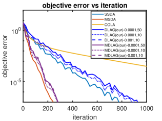
Figure 1: Iteration complexities on heart dataset. DLAG-$0.0001,10$ means DLAG with $\gamma=c=0.0001$ and $D=10$.

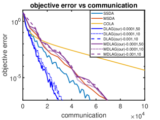
Figure 2: Communication complexities on heart dataset.

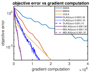
Figure 3: Stochastic gradient complexities on heart dataset.

From Figures 1, 2, and 3, we can see that the behaviors of tested algorithms match Table I.

1. The performance of DLAG and MDLAG is robust to the choice of parameters.

2. DLAG and MDLAG achieve iteration complexities similar to those of SSDA and MSDA, respectively.

3. DLAG still uses the least communication (about $40\%$ less than SSDA).

4. MDLAG has the smallest gradient complexity (about $80\%$ less than MSDA).

VI Conclusions and future work

In this work, we propose DLAG and MDLAG for decentralized machine learning, where computation is saved by applying highly approximate dual gradients, and unnecessary communication can be skipped based on a dynamic criterion. Compared with other methods, DLAG does not rely on extra oracles to compute exact dual gradients or proximal mappings, and successfully reduces communication complexity. All these claims are justified numerically.

There are still open problems to be addressed. For example, can we also apply the worker’s lazy condition for all $K$ rounds of communication in MDLAG, so that it can enjoy least amount of computation and communication?

-A Proof of Lemma 1: error propagating dynamics

Proof.

The inexact dual gradient $\theta^{k}_{i}$ is produced by solving the following subproblem by Katyusha:

$$\begin{split}\theta^{k}_{i}&\approx\operatorname*{arg\,min}_{\theta\in\operatorname*{\mathbb{R}^{d}}}\{\frac{1}{m}\sum_{j=1}^{m}\left(f_{i,j}(\theta)-\langle\theta,x^{k}_{i}\rangle\right)\}.\end{split}$$ (15)

We will apply Katyusha such that the inexact dual gradient $\theta^{k}_{i}$ satisfies

$$\mathbb{E}_{k}\|\theta^{k}_{i}-\nabla f^{*}_{i}(x^{k}_{i})\|^{2}\leq\frac{c}{2}\|\theta^{k-1}_{i}-\nabla f^{*}_{i}(x^{k}_{i})\|^{2},$$ (16)

where $\nabla f^{*}_{i}(x^{k}_{i})$ is the solution of (15).

Denote $F_{i}(\theta)=f_{i}(\theta)-\langle\theta,x^{k}_{i}\rangle$. By Theorem 3.1 of [4], we know that if Katyusha is warm started at $\theta^{k-1}_{i}$, Katyusha needs

$$\mathcal{O}\left((m+\sqrt{m\kappa_{i}})\log(\frac{F_{i}(\theta^{k-1}_{i})-F_{i}(\nabla f^{*}_{i}(x^{k}_{i}))}{\varepsilon_{0}})\right)$$

stochastic gradient evaluations in expectation to reach

$$\mathbb{E}_{k}[F_{i}(\theta^{k}_{i})-F_{i}(\nabla f^{*}_{i}(x^{k}_{i}))]\leq\varepsilon_{0}.$$ (17)

Here, if we take

$$\varepsilon_{0}=\frac{\mu_{i}c}{4}\|\theta^{k-1}_{i}-\nabla f^{*}_{i}(x^{k}_{i})\|^{2}.$$ (18)

then we obtain a stochastic gradient complexity of

$$\mathcal{O}\left((m+\sqrt{m\kappa_{i}})\log(\frac{4}{\mu_{i}c}\frac{F_{i}(\theta^{k-1}_{i})-F_{i}(\nabla f^{*}_{i}(x^{k}_{i}))}{\|\theta^{k-1}_{i}-\nabla f^{*}_{i}(x^{k}_{i})\|^{2}})\right)$$

$$=\mathcal{O}\left((m+\sqrt{m\kappa_{i}})\log(\frac{2\kappa_{\mathrm{max}}}{c})\right).$$

On the other hand, from (17) and (18) we have

$$\mathbb{E}_{k}\|\theta^{k}_{i}-\nabla f^{*}_{i}(x^{k}_{i})\|^{2}\leq\frac{c}{2}\|\theta^{k-1}_{i}-\nabla f^{*}_{i}(x^{k}_{i})\|^{2},$$

which is exactly (16).

Furthermore, (16) leads to

$$\begin{split}\mathbb{E}_{k}\|\theta^{k}_{i}-\nabla f^{*}_{i}(x^{k}_{i})\|^{2}&\leq c\|\theta^{k-1}_{i}-\nabla f^{*}_{i}(x^{k-1}_{i})\|^{2}\\ &\quad+c\|\nabla f^{*}_{i}(x^{k}_{i})-\nabla f^{*}_{i}(x^{k-1}_{i})\|^{2}.\end{split}$$ (19)

Define $a^{k}_{i}=\operatorname*{\mathbb{E}}\|\theta^{k}_{i}-\nabla f^{*}_{i}(x^{k}_{i})\|^{2}$ and $b^{k}_{i}=\operatorname*{\mathbb{E}}\|\nabla f^{*}_{i}(x^{k}_{i})-\nabla f^{*}_{i}(x^{k-1}_{i})\|^{2}$. Then, (19) becomes the following recursion:

$$\frac{a_{i}^{k}}{c^{k}}-\frac{a^{k-1}_{i}}{c^{k-1}}\leq\frac{b^{k-1}_{i}}{c^{k-1}},$$

Since $a^{0}_{i}=\|\theta^{0}_{i}-\nabla f^{*}_{i}(x^{0}_{i})\|^{2}=0$, we have $\frac{a^{k}_{i}}{c^{k}}\leq\sum_{j=0}^{k-1}\frac{b^{j}_{i}}{c^{j}}$, or equivalently,

$$\operatorname*{\mathbb{E}}\|\theta^{k}_{i}-\nabla f^{*}_{i}(x^{k}_{i})\|^{2}\leq\sum_{j=0}^{k-1}c^{k-j}\operatorname*{\mathbb{E}}\|\nabla f^{*}_{i}(x^{j}_{i})-\nabla f^{*}_{i}(x^{j+1}_{i})\|^{2}.$$ (20)

The desired result follows. ∎

-B Gradient error bound

In this section, we prove a lemma on the gradient error.

Lemma 2 (Gradient error).

Under the same settings as in Lemma 1, the difference between $\hat{\Theta}^{k}\sqrt{U}$ and the true gradient $g^{k}\coloneqq\nabla F^{*}({\xi}^{k}\sqrt{U})\sqrt{U}$ satisfies:

$$\begin{split}&\operatorname*{\mathbb{E}}\|\hat{\Theta}^{k}\sqrt{U}-g^{k}\|^{2}\\ &\leq 6\|\sqrt{U}\|^{4}\sum_{j=0}^{k-D-1}\frac{c^{k-D-j}}{\mu^{2}_{\mathrm{min}}}\operatorname*{\mathbb{E}}\|\xi^{j}_{i}-\xi^{j+1}_{i}\|^{2}\\ &\quad+8\|\sqrt{U}\|^{4}\sum_{j=0}^{k-1}\frac{c^{k-j}}{\mu^{2}_{\mathrm{min}}}\operatorname*{\mathbb{E}}\|\xi^{j}-\xi^{j+1}\|^{2}\\ &\quad+6\|\sqrt{U}\|^{4}\sum_{j=k-D}^{k-1}\frac{c}{\mu^{2}_{\mathrm{min}}}\operatorname*{\mathbb{E}}\|\xi^{j}-\xi^{j+1}\|^{2}\\ &\quad+6\|\sqrt{U}\|^{4}\sum_{j=k-D}^{k-1}\frac{\gamma}{\mu^{2}_{\mathrm{min}}}\operatorname*{\mathbb{E}}\|\xi^{j}-\xi^{j+1}\|^{2},\end{split}$$ (21)

Proof.

First of all, we have

$$\|\hat{\Theta}^{k}\sqrt{U}-g^{k}\|^{2} \leq 2\|(\hat{\Theta}^{k}-\Theta^{k})\sqrt{U}\|^{2}$$

$$\quad+2\|\Theta^{k}\sqrt{U}-\nabla F^{*}(x^{k})\sqrt{U}\|^{2}.$$ (22)

In DLAG, if worker $i$’s lazy condition (8) is satisfied, then $\hat{\theta}^{k}_{i}=\hat{\theta}^{k-1}_{i}$ (skipping communication), and $\hat{\theta}^{k}_{i}={\theta}^{k}_{i}$ (perform communication) otherwise. As a result, we have

$$\begin{split}\|\hat{\theta}^{k}_{i}-\theta^{k}_{i}\|^{2}&\leq 3\sum_{j=0}^{k-D-1}\frac{c^{k-D-j}}{\mu^{2}_{\mathrm{min}}}\|x^{j}_{i}-x^{j+1}_{i}\|^{2}\\ &\quad+3\sum_{j=0}^{k-1}\frac{c^{k-j}}{\mu^{2}_{\mathrm{min}}}\|x^{j}_{i}-x^{j+1}_{i}\|^{2}\\ &\quad+3\sum_{j=k-D}^{k-1}\frac{c}{\mu^{2}_{\mathrm{min}}}\|x^{j}_{i}-x^{j+1}_{i}\|^{2}\\ &\quad+3\sum_{j=k-D}^{k-1}\frac{\gamma}{\mu^{2}_{\mathrm{min}}}\|x^{j}_{i}-x^{j+1}_{i}\|^{2}.\end{split}$$

In view of this, the first term on the right hand side of (-B) can be then bounded as

$$\begin{split}&2\|(\hat{\Theta}^{k}-\Theta^{k})\sqrt{U}\|^{2}\\ &\leq 2\|\sqrt{U}\|^{2}\|\hat{\Theta}^{k}-\Theta^{k}\|^{2}\\ &\leq 6\|\sqrt{U}\|^{4}\sum_{j=0}^{k-D-1}\frac{c^{k-D-j}}{\mu^{2}_{\mathrm{min}}}\|\xi^{j}_{i}-\xi^{j+1}_{i}\|^{2}\\ &\quad+6\|\sqrt{U}\|^{4}\sum_{j=0}^{k-1}\frac{c^{k-j}}{\mu^{2}_{\mathrm{min}}}\|\xi^{j}-\xi^{j+1}\|^{2}\\ &\quad+6\|\sqrt{U}\|^{4}\sum_{j=k-D}^{k-1}\frac{c}{\mu^{2}_{\mathrm{min}}}\|\xi^{j}-\xi^{j+1}\|^{2}\\ &\quad+6\|\sqrt{U}\|^{4}\sum_{j=k-D}^{k-1}\frac{\gamma}{\mu^{2}_{\mathrm{min}}}\|\xi^{j}-\xi^{j+1}\|^{2},\end{split}$$ (23)

where we have applied $x=\xi\sqrt{U}$ in the second inequality.

To bound the second term on the right hand side of (-B), we can apply Lemma 1 in the following way:

$$\begin{split}&2\|\Theta^{k}\sqrt{U}-\nabla F^{*}(x^{k})\sqrt{U}\|^{2}\\ &\leq 2\|\sqrt{U}\|^{2}\sum_{j=0}^{k-1}c^{k-j}\operatorname*{\mathbb{E}}\|\nabla F^{*}(x^{j})-\nabla F^{*}(x^{j+1})\|^{2}\\ &\leq 2\|\sqrt{U}\|^{2}\sum_{j=0}^{k-1}\frac{c^{k-j}}{\mu^{2}_{\mathrm{min}}}\operatorname*{\mathbb{E}}\|x^{j}-x^{j+1}\|^{2}\\ &\leq 2\|\sqrt{U}\|^{4}\sum_{j=0}^{k-1}\frac{c^{k-j}}{\mu^{2}_{\mathrm{min}}}\operatorname*{\mathbb{E}}\|\xi^{j}-\xi^{j+1}\|^{2}\end{split}$$ (24)

where we have applied the $\frac{1}{\mu_{\mathrm{min}}}-$smoothness of $F^{*}$ in the first inequality, and $x=\xi\sqrt{U}$ in the second inequality.

Finally, combining (-B), (23), and (24) yields the desired result. ∎

-C Preliminary propositions

First, let us define $\Delta v^{k}\coloneqq v^{k}-\xi^{\star}$ and $\Delta\xi^{k}\coloneqq\xi^{k}-\xi^{\star}.$ Then, the Lyapunov function $L^{k}$ in (IV) can be written as

$$L^{k}=2\eta s\kappa\left(G(\lambda^{k})-G(\xi^{\star})\right)+\|\Delta v^{k}\|^{2}+A^{k}+\tilde{A}^{k},$$

where

$$v^{k} =\xi^{k}+\sqrt{s\kappa}(\xi^{k}-\lambda^{k}),$$ (25)

$$A^{k} =\sum\limits_{d=1}^{D}c_{d}\|\xi^{k+1-d}-\xi^{k-d}\|^{2},$$ (26)

$$\tilde{A}^{k} =\sum\limits_{d=1}^{k}\tilde{c}_{d}\|\xi^{k+1-d}-\xi^{k-d}\|^{2}.$$ (27)

We want to obtain $L^{k+1}-(1-\frac{1}{\sqrt{s\kappa}})L^{k}\leq 0$ for some $s\geq 1$. For this purpose, we bound the terms in $L^{k+1}$ in the following propositions. Their proofs can be found in Appendices -C2, -C3, and -C4, respectively.

Proposition 2.

We have

$$G(\lambda^{k+1}) \leq G(\xi^{k})-\left(\eta-\frac{\eta^{2}\beta}{2}-\frac{\eta^{2}\sqrt{s\kappa}\alpha}{2\rho}\right)\|\hat{\Theta}^{k}\sqrt{U}\|^{2}$$

$$\quad+\frac{\rho}{2\sqrt{s\kappa}\alpha}\|\hat{\Theta}^{k}\sqrt{U}-g^{k}\|^{2}.$$

Proposition 3.

We have

$$\|\Delta v^{k+1}\|^{2}$$

$$\leq\left(1-\frac{1}{\sqrt{s\kappa}}\right)\|\Delta v^{k}\|^{2}$$

$$\ \ \ +\left(\frac{1}{\sqrt{s\kappa}}-\eta\alpha\sqrt{s\kappa}\left(1-\frac{1}{\rho}\right)\right)\|\xi^{k}-\xi^{\star}\|^{2}$$

$$\ \ \ \ +\left(1-\frac{1}{\sqrt{s\kappa}}\right)\left(-\frac{1}{\sqrt{s\kappa}}+\eta\alpha\left(\frac{\sqrt{s\kappa}-1}{\rho}-1\right)\right)\|v^{k}-\xi^{k}\|^{2}$$

$$\ \ \ \ +2\eta s\kappa\left(\left(G(\xi^{\star})-G(\xi^{k})\right)+(1-\frac{1}{\sqrt{s\kappa}})\left(G(\lambda^{k})-G(\xi^{\star})\right)\right)$$

$$\ \ \ \ +\eta^{2}s\kappa\|\hat{\Theta}^{k}\sqrt{U}\|^{2}+2\rho\frac{\eta\sqrt{s\kappa}}{\alpha}\|\hat{\Theta}^{k}\sqrt{U}-g^{k}\|^{2}.$$

Proposition 4.

Let $c_{d}=\sum\limits_{j=d}^{D}(1-\frac{1}{\sqrt{s\kappa}})^{d-j-1}q$ and $q>0$ for $d=1,2,...,D$. Then, we have $c_{d+1}-(1-\frac{1}{\sqrt{s\kappa}})c_{d}=-q$ and

$$A^{k+1}-(1-\frac{1}{\sqrt{s\kappa}})A^{k} \leq 2c_{1}\left(\frac{\sqrt{s\kappa}-1}{\sqrt{s\kappa}(\sqrt{s\kappa}+1)}\right)^{2}\|v^{k}-\xi^{k}\|^{2}$$

$$\quad+2c_{1}\left(\frac{2\eta\sqrt{s\kappa}}{\sqrt{s\kappa}+1}\right)^{2}\|\hat{\Theta}^{k}\sqrt{U}\|^{2}$$

$$\ \ \ \ -\sum\limits_{d=1}^{D}q\|\xi^{k+1-d}-\xi^{k-d}\|^{2}.$$

Similarly, we have

$$\tilde{A}^{k+1}-(1-\frac{1}{\sqrt{s\kappa}})\tilde{A}^{k}$$

$$\leq 2\tilde{c}_{1}\left(\frac{\sqrt{s\kappa}-1}{\sqrt{s\kappa}(\sqrt{s\kappa}+1)}\right)^{2}\|v^{k}-\xi^{k}\|^{2}$$

$$\quad+2\tilde{c}_{1}\left(\frac{2\eta\sqrt{s\kappa}}{\sqrt{s\kappa}+1}\right)^{2}\|\hat{\Theta}^{k}\sqrt{U}\|^{2}$$

$$\ \ \ \ +\sum\limits_{d=1}^{k}(\tilde{c}_{d+1}-(1-\frac{1}{\sqrt{s\kappa}})\tilde{c}_{d})\|\xi^{k+1-d}-\xi^{k-d}\|^{2}.$$

-C1 A toolkit for proof

Before diving into the details of proof of our main theory, let us first list some useful equalities and inequalities.

We will use $g^{k}=\nabla F^{*}(\xi^{k}\sqrt{U})\sqrt{U}$ throughout the rest of the proof.

1. For $v^{k}$ defined in (25), we have

   $$v^{k+1} =(1+\sqrt{s\kappa})\xi^{k+1}-\sqrt{s\kappa}\lambda^{k+1}$$

   $$=(1+\sqrt{s\kappa})\left(\lambda^{k+1}+\frac{\sqrt{s\kappa}-1}{\sqrt{s\kappa}+1}(\lambda^{k+1}-\lambda^{k})\right)$$

   $$\quad-\sqrt{s\kappa}\lambda^{k+1}$$

   $$=\sqrt{s\kappa}\lambda^{k+1}-(\sqrt{s\kappa}-1)\lambda^{k}$$

   $$=\sqrt{s\kappa}(\xi^{k}-\eta\hat{\Theta}^{k}\sqrt{U})$$

   $$\quad-(\sqrt{s\kappa}-1)\left(\left(1+\frac{1}{\sqrt{s\kappa}}\right)\xi^{k}-\frac{1}{\sqrt{s\kappa}}v^{k}\right)$$

   $$=\left(1-\frac{1}{\sqrt{s\kappa}}\right)v^{k}+\frac{1}{\sqrt{s\kappa}}\xi^{k}-\eta\sqrt{s\kappa}\hat{\Theta}^{k}\sqrt{U}.$$ (28)

2. (Young’s inequality) For any $a,b\in\mathbb{R}$ and $\chi>0$, we have

   $$ab\leq\frac{\chi a^{2}}{2}+\frac{b^{2}}{2\chi}.$$ (29)

3. By Proposition 1, for any $\xi_{1},\xi_{2}\in\operatorname*{\mathbb{R}}^{d\times n}$, we have

   $$G(\xi_{2}) \leq G(\xi_{1})+\langle\nabla G(\xi_{1}),\xi_{2}-\xi_{1}\rangle+\frac{\beta}{2}\|\xi_{2}-\xi_{1}\|^{2},$$ (30)

   $$G(\xi_{2}) \geq G(\xi_{1})+\langle\nabla G(\xi_{1}),\xi_{2}-\xi_{1}\rangle+\frac{\alpha}{2}\|\xi_{2}-\xi_{1}\|^{2}.$$ (31)

4. For any $0\leq r\leq 1$ and $x,y\in\operatorname*{\mathbb{R}^{n}}$, we have

   $$\|(1-r)x+ry\|^{2} =(1-r)\|x\|^{2}+r\|y\|^{2}$$

   $$\quad-r(1-r)\|x-y\|^{2}.$$ (32)

5. For any $0\leq x\leq\frac{1}{2},y\geq 0$, we have

   $$(1-x)^{-y}\leq e^{2xy}.$$ (33)

-C2 Proof of Proposition 2

We have

$$G(\lambda^{k+1})=G(\xi^{k}-\eta\hat{\Theta}^{k}\sqrt{U})$$

$$\overset{(a)}{\leq}G(\xi^{k})-\eta\langle g^{k},\hat{\Theta}^{k}\sqrt{U}\rangle+\frac{\eta^{2}\beta}{2}\|\hat{\Theta}^{k}\sqrt{U}\|^{2}$$

$$=G(\xi^{k})-\eta\|\hat{\Theta}^{k}\sqrt{U}\|^{2}+\eta\langle\hat{\Theta}^{k}\sqrt{U}-g^{k},\hat{\Theta}^{k}\sqrt{U}\rangle$$

$$\quad+\frac{\eta^{2}\beta}{2}\|\hat{\Theta}^{k}\sqrt{U}\|^{2}$$

$$\overset{(b)}{\leq}G(\xi^{k})-\left(\eta-\frac{\eta^{2}\beta}{2}-\frac{\eta^{2}\sqrt{s\kappa}\alpha}{2\rho}\right)\|\hat{\Theta}^{k}\sqrt{U}\|^{2}$$

$$\quad+\frac{\rho}{2\sqrt{s\kappa}\alpha}\|\hat{\Theta}^{k}\sqrt{U}-g^{k}\|^{2},$$

where $(a)$ follows from the smoothness of $G$ in (30), $(b)$ follows from (29) with $\chi=\frac{\rho}{\eta\sqrt{s\kappa}\alpha}$, and $\rho>0$ will be determined later.

-C3 Proof of Proposition 3

Equation (25) implies that

$$\Delta v^{k+1}=\left(1-\frac{1}{\sqrt{s\kappa}}\right)\Delta v^{k}+\frac{1}{\sqrt{s\kappa}}\Delta\xi^{k}-\eta\sqrt{s\kappa}\hat{\Theta}^{k}\sqrt{U}.$$

Therefore,

$$\|\Delta v^{k+1}\|^{2}$$

$$=\left\|\left(1-\frac{1}{\sqrt{s\kappa}}\right)\Delta v^{k}+\frac{1}{\sqrt{s\kappa}}\Delta\xi^{k}\right\|^{2}+\eta^{2}s\kappa\|\hat{\Theta}^{k}\sqrt{U}\|^{2}$$

$$\quad-2\eta\sqrt{s\kappa}\left\langle\left(1-\frac{1}{\sqrt{s\kappa}}\right)\Delta v^{k}+\frac{1}{\sqrt{s\kappa}}\Delta\xi^{k},\hat{\Theta}^{k}\sqrt{U}\right\rangle$$

$$\overset{(a)}{=}\left(1-\frac{1}{\sqrt{s\kappa}}\right)\|\Delta v^{k}\|^{2}+\frac{1}{\sqrt{s\kappa}}\|\Delta\xi^{k}\|^{2}$$

$$\quad-\left(1-\frac{1}{\sqrt{s\kappa}}\right)\frac{1}{\sqrt{s\kappa}}\|v^{k}-\xi^{k}\|^{2}+\eta^{2}s\kappa\|\hat{\Theta}^{k}\sqrt{U}\|^{2}$$

$$\ \ \ -2\eta\sqrt{s\kappa}\left\langle\left(1-\frac{1}{\sqrt{s\kappa}}\right)\Delta v^{k}+\frac{1}{\sqrt{s\kappa}}\Delta\xi^{k},\hat{\Theta}^{k}\sqrt{U}\right\rangle$$

$$\overset{(b)}{=}\left(1-\frac{1}{\sqrt{s\kappa}}\right)\|\Delta v^{k}\|^{2}+\frac{1}{\sqrt{s\kappa}}\|\Delta\xi^{k}\|^{2}$$

$$\quad-\left(1-\frac{1}{\sqrt{s\kappa}}\right)\frac{1}{\sqrt{s\kappa}}\|v^{k}-\xi^{k}\|^{2}+\eta^{2}s\kappa\|\hat{\Theta}^{k}\sqrt{U}\|^{2}$$

$$\ \ \ -2\eta\sqrt{s\kappa}\langle\Delta\xi^{k}+(\sqrt{s\kappa}-1)(\xi^{k}-\lambda^{k}),\hat{\Theta}^{k}\sqrt{U}\rangle$$

where $(a)$ follows from (4) and $\Delta v^{k}-\Delta\xi^{k}=v^{k}-\xi^{k}$, $(b)$ follows from the definition of $v^{k}$ in (25).

For $-\langle\Delta\xi^{k},\hat{\Theta}^{k}\sqrt{U}\rangle$ we have

$$-\langle\Delta\xi^{k},\hat{\Theta}^{k}\sqrt{U}\rangle$$

$$=-\langle\Delta\xi^{k},g^{k}\rangle-\langle\Delta\xi^{k},\hat{\Theta}^{k}\sqrt{U}-g^{k}\rangle$$

$$\overset{(c)}{\leq}G(\xi^{\star})-G(\xi^{k})-\frac{\alpha}{2}\|\Delta\xi^{k}\|^{2}-\langle\Delta\xi^{k},\hat{\Theta}^{k}\sqrt{U}-g^{k}\rangle$$

$$\overset{(d)}{\leq}G(\xi^{\star})-G(\xi^{k})-\frac{\alpha}{2}\|\Delta\xi^{k}\|^{2}+\frac{\rho}{2\alpha}\|\hat{\Theta}^{k}\sqrt{U}-g^{k}\|^{2}$$

$$\quad+\frac{\alpha}{2\rho}\|\Delta\xi^{k}\|^{2}.$$

where (c) follows from the strong convexity of $G$ in (31), and (d) follows from Young’s inequality (29) with $\chi=\frac{\rho}{\alpha}$.

Similarly, for $-\langle\xi^{k}-\lambda^{k},\hat{\Theta}^{k}\sqrt{U}\rangle$ we have

$$-\langle\xi^{k}-\lambda^{k},\hat{\Theta}^{k}\sqrt{U}\rangle$$

$$=-\langle\xi^{k}-\lambda^{k},g^{k}\rangle-\langle\xi^{k}-\lambda^{k},\hat{\Theta}^{k}\sqrt{U}-g^{k}\rangle$$

$$\leq G(\lambda^{k})-G(\xi^{k})-\frac{\alpha}{2}\|\xi^{k}-\lambda^{k}\|^{2}$$

$$\quad+\frac{\rho}{2(\sqrt{s\kappa}-1)\alpha}\|\hat{\Theta}^{k}\sqrt{U}-g^{k}\|^{2}$$

$$\quad+\frac{(\sqrt{s\kappa}-1)\alpha}{2\rho}\|\xi^{k}-\lambda^{k}\|^{2}$$

$$=G(\lambda^{k})-G(\xi^{k})$$

$$\quad-\frac{1}{s\kappa}\left(\frac{\alpha}{2}-\frac{(\sqrt{s\kappa}-1)\alpha}{2\rho}\right)\|v^{k}-\xi^{k}\|^{2}$$

$$\quad+\frac{\rho}{2(\sqrt{s\kappa}-1)\alpha}\|\hat{\Theta}^{k}\sqrt{U}-g^{k}\|^{2}.$$

where the last equality follows from (25).

As a result,

$$\|\Delta v^{k+1}\|^{2}$$

$$\leq\left(1-\frac{1}{\sqrt{s\kappa}}\right)\|\Delta v^{k}\|^{2}+\frac{1}{\sqrt{s\kappa}}\|\Delta\xi^{k}\|^{2}$$

$$\quad-\left(1-\frac{1}{\sqrt{s\kappa}}\right)\frac{1}{\sqrt{s\kappa}}\|v^{k}-\xi^{k}\|^{2}+\eta^{2}s\kappa\|\hat{\Theta}^{k}\sqrt{U}\|^{2}$$

$$\ \ \ \ +2\eta\sqrt{s\kappa}\bigg{(}G(\xi^{\star})-G(\xi^{k})-\frac{\alpha}{2}\left(1-\frac{1}{\rho}\right)\|\Delta\xi^{k}\|^{2}$$

$$\quad\quad\quad\quad\quad+\frac{\rho}{2\alpha}\|\hat{\Theta}^{k}\sqrt{U}-g^{k}\|^{2}\bigg{)}$$

$$\ \ \ \ +2\eta\sqrt{s\kappa}(\sqrt{s\kappa}-1)$$

$$\quad\times\bigg{(}G(\lambda^{k})-G(\xi^{k})-\frac{1}{s\kappa}\frac{\alpha}{2}\left(1-\frac{\sqrt{s\kappa}-1}{\rho}\right)\|v^{k}-\xi^{k}\|^{2}$$

$$\quad\quad\quad+\frac{\rho}{2(\sqrt{s\kappa}-1)\alpha}\|\hat{\Theta}^{k}\sqrt{U}-g^{k}\|^{2}\bigg{)}$$

$$=\left(1-\frac{1}{\sqrt{s\kappa}}\right)\|\Delta v^{k}\|^{2}+\left(\frac{1}{\sqrt{s\kappa}}-\eta\alpha\sqrt{s\kappa}\left(1-\frac{1}{\rho}\right)\right)\|\Delta\xi^{k}\|^{2}$$

$$+\left(1-\frac{1}{\sqrt{s\kappa}}\right)\left(-\frac{1}{\sqrt{s\kappa}}+\eta\alpha\left(\frac{\sqrt{s\kappa}-1}{\rho}-1\right)\right)\|v^{k}-\xi^{k}\|^{2}$$

$$+2\eta s\kappa\left(\left(G(\xi^{\star})-G(\xi^{k})\right)+(1-\frac{1}{\sqrt{s\kappa}})\left(G(\lambda^{k})-G(\xi^{\star})\right)\right)$$

$$+\eta^{2}s\kappa\|\hat{\Theta}^{k}\sqrt{U}\|^{2}+2\rho\frac{\eta\sqrt{s\kappa}}{\alpha}\|\hat{\Theta}^{k}\sqrt{U}-g^{k}\|^{2}.$$

-C4 Proof of Proposition 4

Since $c_{d}=\sum\limits_{j=d}^{D}r^{d-j-1}q$, where $r=1-\frac{1}{\sqrt{s\kappa}}$ and $q>0$, we have

$$A_{k+1}-rA_{k}$$

$$=c_{1}\|\xi^{k+1}-\xi^{k}\|^{2}+\sum\limits_{d=1}^{D-1}(c_{d+1}-rc_{d})\|\xi^{k+1-d}-\xi^{k-d}\|^{2}$$

$$\quad-rc_{D}\|\xi^{k+1-D}-\xi^{k-D}\|^{2}$$

$$=c_{1}\|\xi^{k+1}-\xi^{k}\|^{2}-\sum\limits_{d=1}^{D}q\|\xi^{k+1-d}-\xi^{k-d}\|^{2}.$$

To deal with $\xi^{k+1}-\xi^{k}$, we can write

$$\xi^{k+1}-\xi^{k}$$

$$=\lambda^{k+1}-\xi^{k}+\frac{\sqrt{s\kappa}-1}{\sqrt{s\kappa}+1}(\lambda^{k+1}-\xi^{k}+\xi^{k}-\lambda^{k})$$

$$=-\eta\hat{\Theta}^{k}\sqrt{U}+\frac{\sqrt{s\kappa}-1}{\sqrt{s\kappa}+1}(-\eta\hat{\Theta}^{k}\sqrt{U})$$

$$\quad+\frac{\sqrt{s\kappa}-1}{\sqrt{s\kappa}+1}\frac{1}{\sqrt{s\kappa}}(v^{k}-\xi^{k})$$

$$=\frac{1}{1+\sqrt{s\kappa}}\left((1-\frac{1}{\sqrt{s\kappa}})(v^{k}-\xi^{k})-2\eta\sqrt{s\kappa}\hat{\Theta}^{k}\sqrt{U}\right).$$

Therefore,

$$A_{k+1}-rA_{k}$$

$$=c_{1}\left\|\frac{1}{1+\sqrt{s\kappa}}\left((1-\frac{1}{\sqrt{s\kappa}})(v^{k}-\xi^{k})-2\eta\sqrt{s\kappa}\hat{\Theta}^{k}\sqrt{U}\right)\right\|^{2}$$

$$\quad-\sum\limits_{d=1}^{D}q\|\xi^{k+1-d}-\xi^{k-d}\|^{2}$$

$$\leq 2c_{1}\left(\frac{\sqrt{s\kappa}-1}{\sqrt{s\kappa}(\sqrt{s\kappa}+1)}\right)^{2}\|v^{k}-\xi^{k}\|^{2}$$

$$\quad+2c_{1}\left(\frac{2\eta\sqrt{s\kappa}}{\sqrt{s\kappa}+1}\right)^{2}\|\hat{\Theta}^{k}\sqrt{U}\|^{2}-\sum\limits_{d=1}^{D}q\|\xi^{k+1-d}-\xi^{k-d}\|^{2}.$$

Similarly, we also have

$$\tilde{A}_{k+1}-r\tilde{A}_{k}$$

$$=\tilde{c}_{1}\|\xi^{k+1}-\xi^{k}\|^{2}+\sum\limits_{d=1}^{k}(\tilde{c}_{d+1}-r\tilde{c}_{d})\|\xi^{k+1-d}-\xi^{k-d}\|^{2}$$

$$=\tilde{c}_{1}\left\|\frac{1}{1+\sqrt{s\kappa}}\left((1-\frac{1}{\sqrt{s\kappa}})(v^{k}-\xi^{k})-2\eta\sqrt{s\kappa}\hat{\Theta}^{k}\sqrt{U}\right)\right\|^{2}$$

$$\quad+\sum\limits_{d=1}^{k}(\tilde{c}_{d+1}-r\tilde{c}_{d})\|\xi^{k+1-d}-\xi^{k-d}\|^{2}$$

$$\leq 2\tilde{c}_{1}\left(\frac{\sqrt{s\kappa}-1}{\sqrt{s\kappa}(\sqrt{s\kappa}+1)}\right)^{2}\|v^{k}-\xi^{k}\|^{2}$$

$$\quad+2c_{1}\left(\frac{2\eta\sqrt{s\kappa}}{\sqrt{s\kappa}+1}\right)^{2}\|\hat{\Theta}^{k}\sqrt{U}\|^{2}$$

$$\quad+\sum\limits_{d=1}^{k}(\tilde{c}_{d+1}-r\tilde{c}_{d})\|\xi^{k+1-d}-\xi^{k-d}\|^{2}.$$

-D Stochastic Gradient complexity

In order to prove Theorem 1 directly follows, we prove a slightly more general result stated in Theorem 4.

Theorem 4.

Take Assumptions 1 and 2, and let $\sqrt{\kappa_{\mathrm{max}}}\log(\frac{128\kappa^{3}_{\mathrm{max}}}{c})$, and

$$\eta=\frac{\sqrt{2+\frac{1}{12(a+b)}}}{1+\sqrt{2+\frac{1}{12(a+b)}}}\frac{1}{1+24(a+b)(2+\sqrt{2+\frac{1}{12(a+b)}})}\frac{1}{\beta},$$

$$s=\frac{2+\sqrt{2+\frac{1}{12(a+b)}}}{\sqrt{2+\frac{1}{12(a+b)}}}\left(1+24(a+b)\left(2+\sqrt{2+\frac{1}{12(a+b)}}\right)\right),$$

where $a=\frac{6\|\sqrt{U}\|^{4}}{\alpha\beta\mu^{2}_{\mathrm{min}}}\gamma De^{\frac{2D}{\sqrt{\kappa}}}$ and $b=\frac{25\|\sqrt{U}\|^{4}}{\alpha\beta\mu^{2}_{\mathrm{min}}}cDe^{\frac{2D}{\sqrt{\kappa}}}$, where $\kappa=\frac{\kappa_{F}}{\zeta_{U}}$. Assume that $\kappa>2$. At each iteration, let the subproblem (7) be solved by Katyusha with $\mathcal{O}(m+\sqrt{m\kappa_{\mathrm{max}}})$ stochastic gradient evaluations. Then, we have $\operatorname*{\mathbb{E}}[L^{k+1}]\leq\left(1-\frac{1}{\sqrt{s\kappa}}\right)\operatorname*{\mathbb{E}}[L^{k}]$ for any $k\geq 0$. Therefore, in order to obtain an approximate solution to (4) with $\varepsilon-$suboptimality, Algorithm 2 has an iteration complexity of

$$\mathcal{I}_{\mathrm{DLAG}}(\varepsilon)=\mathcal{O}\left(\sqrt{s\kappa}\log(\frac{1}{\varepsilon})\right),$$

in expectation, and a stochastic gradient complexity of

$$\mathcal{G}_{\mathrm{DLAG}}(\varepsilon)=\mathcal{O}\left((m+\sqrt{m\kappa_{\mathrm{max}}})\sqrt{s\kappa}\log(\frac{1}{\varepsilon})\right).$$

in expectation.

-E Proof of Theorem 4

Combining Propositions 2, 3, and 4 with the definition of $L^{k}$ in (IV) yields

$$\begin{split}&\ \ \ L^{k+1}-\left(1-\frac{1}{\sqrt{s\kappa}}\right)L^{k}\\ &\leq\|\Delta\xi^{k}\|^{2}\times C_{1}+\|v^{k}-\xi^{k}\|^{2}\times C_{2}\\ &\ \ \ +\|\hat{\Theta}^{k}\sqrt{U}\|^{2}\times C_{3}\\ &\ \ \ +\|\hat{\Theta}^{k}\sqrt{U}-g^{k}\|^{2}\times(3\rho\sqrt{s\kappa}\eta\frac{1}{\alpha})\\ &\ \ \ +\sum\limits_{d=1}^{D}\|\xi^{k+1-d}-\xi^{k-d}\|^{2}\times\left(-q\right)\\ &\ \ \ +\sum\limits_{d=1}^{k}\|\xi^{k+1-d}-\xi^{k-d}\|^{2}\times\left(\tilde{c}_{d+1}-r\tilde{c}_{d}\right)\end{split}$$

where the coefficients $C_{1},C_{2}$, and $C_{3}$ are

$$\begin{split}C_{1}&=\left(\frac{1}{\sqrt{s\kappa}}-\eta\alpha\sqrt{s\kappa}\left(1-\frac{1}{\rho}\right)\right),\\ C_{2}&=\Bigg{(}\left(1-\frac{1}{\sqrt{s\kappa}}\right)\bigg{(}-\frac{1}{\sqrt{s\kappa}}+\eta\alpha\big{(}\frac{\sqrt{s\kappa}-1}{\rho}-1\big{)}\bigg{)}\\ &\quad\quad\quad\quad\quad\quad\quad\quad\quad\quad\quad+2c_{1}\left(\frac{\sqrt{s\kappa}-1}{\sqrt{s\kappa}(\sqrt{s\kappa}+1)}\right)^{2}\\ &\quad\quad\quad\quad\quad\quad\quad\quad\quad\quad\quad+2\tilde{c}_{1}\left(\frac{\sqrt{s\kappa}-1}{\sqrt{s\kappa}(\sqrt{s\kappa}+1)}\right)^{2}\Bigg{)},\\ C_{3}&=\eta^{2}s\kappa\Bigg{(}-1+2c_{1}\left(\frac{2}{\sqrt{s\kappa}+1}\right)^{2}+2\tilde{c}_{1}\left(\frac{2}{\sqrt{s\kappa}+1}\right)^{2}\\ &\quad\quad\quad\quad\quad\quad\quad\quad\quad\quad\quad+\left(\eta\beta+\frac{\eta\alpha\sqrt{s\kappa}}{\rho}\right)\Bigg{)}.\end{split}$$ (34)

By Lemma 2 we further know that

$$\begin{split}&\ \ \ \operatorname*{\mathbb{E}}[L^{k+1}-\left(1-\frac{1}{\sqrt{s\kappa}}\right)L^{k}]\\ &\leq C_{1}\operatorname*{\mathbb{E}}\|\Delta\xi^{k}\|^{2}+C_{2}\operatorname*{\mathbb{E}}\|v^{k}-\xi^{k}\|^{2}+C_{3}\operatorname*{\mathbb{E}}\|\hat{\Theta}^{k}\sqrt{U}\|^{2}\\ &\ \ \ +\left(\frac{3\rho\sqrt{s\kappa}\eta}{\alpha}6\|\sqrt{U}\|^{4}\frac{\gamma}{\mu^{2}_{\mathrm{min}}}-q\right)\sum\limits_{d=1}^{D}\operatorname*{\mathbb{E}}\|\xi^{k+1-d}-\xi^{k-d}\|^{2}\\ &\ \ \ +\left(\frac{3\rho\sqrt{s\kappa}\eta}{\alpha}6\|\sqrt{U}\|^{4}\frac{c}{\mu^{2}_{\mathrm{min}}}\right)\sum\limits_{d=1}^{D}\operatorname*{\mathbb{E}}\|\xi^{k+1-d}-\xi^{k-d}\|^{2}\\ &\ \ \ +\left(\frac{3\rho\sqrt{s\kappa}\eta}{\alpha}8\|\sqrt{U}\|^{4}\frac{c^{d}}{\mu^{2}_{\mathrm{min}}}\right)\sum\limits_{d=1}^{k}\operatorname*{\mathbb{E}}\|\xi^{k+1-d}-\xi^{k-d}\|^{2}\\ &\ \ \ +\left(\frac{3\rho\sqrt{s\kappa}\eta}{\alpha}6\|\sqrt{U}\|^{4}\frac{c^{d-D}}{\mu^{2}_{\mathrm{min}}}\right)\sum\limits_{d=D+1}^{k}\operatorname*{\mathbb{E}}\|\xi^{k+1-d}-\xi^{k-d}\|^{2}\\ &\ \ \ +\left(\tilde{c}_{d+1}-(1-\frac{1}{\sqrt{s\kappa}})\tilde{c}_{d}\right)\sum\limits_{d=1}^{k}\operatorname*{\mathbb{E}}\|\xi^{k+1-d}-\xi^{k-d}\|^{2}.\end{split}$$ (35)

In the rest of the proof, we will select $\eta,\rho,s$, and $q$ such that the right-hand side of (35) is non-positive. Therefore, $L^{k}$ converges to $0$ at a linear rate of $1-\frac{1}{\sqrt{s\kappa}}$. Recalling the definition of $L^{k}$ in (IV), we know that the (expected) iteration complexity for Algorithm 2 to obtain an $\varepsilon-$suboptimal solution is

$$\mathcal{I}_{\mathrm{DLAG}}=\mathcal{O}\left(\sqrt{s\kappa}\log(\frac{1}{\varepsilon})\right),$$

where $s$ will be specified in (45).

-E1 Bound $c_{1}$ to make the first and fourth term of (35) non-positive

In order for the coefficient $C_{1}$ in (35) and (34) to be non-negative, we can set $\rho>1$ and

$$\eta s\beta\geq\frac{1}{1-\frac{1}{\rho}}=\frac{\rho}{\rho-1}.$$

Therefore, it suffices to set

$$s=\frac{\rho}{\rho-1}\frac{1}{\eta\beta}.$$ (36)

Let us also set $q=\frac{18\rho\eta\|\sqrt{U}\|^{4}}{\alpha\mu^{2}_{\mathrm{min}}}\sqrt{s\kappa}\gamma$ to make the fourth term of (35) to be $0$. Therefore,

$$\begin{split}c_{1}&=\sum\limits_{j=1}^{D}(1-\frac{1}{\sqrt{s\kappa}})^{-j}q\leq qD(1-\frac{1}{\sqrt{s\kappa}})^{-D}\\ &\leq qDe^{\frac{2D}{\sqrt{s\kappa}}}\leq qDe^{\frac{2D}{\sqrt{\kappa}}}\\ &=\frac{18\rho\eta\|\sqrt{U}\|^{4}}{\alpha\mu^{2}_{\mathrm{min}}}\sqrt{s\kappa}\gamma De^{\frac{2D}{\sqrt{\kappa}}}=3a\rho\eta\beta\sqrt{s\kappa}.\end{split}$$ (37)

where the second inequality follows from (33) (note that $\kappa>2$ and $s\geq 1$). In the last equality, we have set

$$a=\frac{6\|\sqrt{U}\|^{4}}{\alpha\beta\mu^{2}_{\mathrm{min}}}\gamma De^{\frac{2D}{\sqrt{\kappa}}}.$$ (38)

-E2 Bound $\tilde{c}_{1}$ to make the sum of last 4 terms of (35) non-positive

Let $r=1-\frac{1}{\sqrt{s\kappa}}$. In order to make the sum of the last four terms to be non-positive, we require that

$$\frac{\tilde{c}_{d}}{r^{d}}-\frac{\tilde{c}_{d+1}}{r^{d+1}}$$

$$=\left(6\frac{c}{r^{d+1}}+8\frac{c^{d}}{r^{d+1}}\right)\frac{\|\sqrt{U}\|^{4}}{\mu^{2}_{\mathrm{min}}}(3\rho\sqrt{s\kappa}\eta\frac{1}{\alpha})\quad\text{for}\,\,1\leq d\leq D,$$

$$\frac{\tilde{c}_{d}}{r^{d}}-\frac{\tilde{c}_{d+1}}{r^{d+1}}$$

$$=\left(6\frac{c^{d-D}}{r^{d+1}}+8\frac{c^{d}}{r^{d+1}}\right)\frac{\|\sqrt{U}\|^{4}}{\mu^{2}_{\mathrm{min}}}(3\rho\sqrt{s\kappa}\eta\frac{1}{\alpha})\quad\text{for}\,\,d\geq D+1.$$

In order to ensure that $\tilde{c}_{d}>0$ for all $d\geq 1$, let us take $\tilde{c}_{1}$ such that

$$\frac{\tilde{c}_{1}}{r} =\sum_{d=D+1}^{\infty}\left(6\frac{c^{d-D}}{r^{d+1}}+8\frac{c^{d}}{r^{d+1}}\right)\frac{\|\sqrt{U}\|^{4}}{\mu^{2}_{\mathrm{min}}}(3\rho\sqrt{s\kappa}\eta\frac{1}{\alpha})$$

$$\ \ \ +\sum_{d=1}^{D}\left(6\frac{c}{r^{d+1}}+8\frac{c^{d}}{r^{d+1}}\right)\frac{\|\sqrt{U}\|^{4}}{\mu^{2}_{\mathrm{min}}}(3\rho\sqrt{s\kappa}\eta\frac{1}{\alpha}).$$

Let $c\leq\frac{r}{2}$, we have

$$\tilde{c}_{1} =\left(6\frac{\frac{c}{r^{D+1}}}{1-\frac{c}{r}}+8\frac{\frac{c^{D+1}}{r^{D+1}}}{1-\frac{c}{r}}\right)\frac{\|\sqrt{U}\|^{4}}{\mu^{2}_{\mathrm{min}}}(3\rho\sqrt{s\kappa}\eta\frac{1}{\alpha})$$

$$\ \ \ +\left(6c\frac{\frac{1}{r}(1-\frac{1}{r^{D}})}{1-\frac{1}{r}}+8\frac{\frac{c}{r}(1-\frac{c^{D}}{r^{D}})}{1-\frac{c}{r}}\right)\frac{\|\sqrt{U}\|^{4}}{\mu^{2}_{\mathrm{min}}}(3\rho\sqrt{s\kappa}\eta\frac{1}{\alpha})$$

$$\leq\left(12\frac{c}{r^{D+1}}+16\frac{c^{D+1}}{r^{D+1}}\right)\frac{\|\sqrt{U}\|^{4}}{\mu^{2}_{\mathrm{min}}}(3\rho\sqrt{s\kappa}\eta\frac{1}{\alpha})$$

$$\ \ \ +\left(6\frac{cD}{r^{D}}+16\frac{c}{r}\right)\frac{\|\sqrt{U}\|^{4}}{\mu^{2}_{\mathrm{min}}}(3\rho\sqrt{s\kappa}\eta\frac{1}{\alpha})$$

$$\leq\left(12\frac{c}{r^{D+1}}+16\frac{1}{2^{D}}\frac{c}{r^{D+1}}\right)\frac{\|\sqrt{U}\|^{4}}{\mu^{2}_{\mathrm{min}}}(3\rho\sqrt{s\kappa}\eta\frac{1}{\alpha})$$

$$\ \ \ +\left(6\frac{cD}{r^{D+1}}+16\frac{c}{r^{D+1}}\right)\frac{\|\sqrt{U}\|^{4}}{\mu^{2}_{\mathrm{min}}}(3\rho\sqrt{s\kappa}\eta\frac{1}{\alpha})$$

where we have applied $\frac{1-\frac{1}{r^{D}}}{1-\frac{1}{r}}=(\frac{1}{r^{D-1}}+...+1)\leq D\frac{1}{r^{D-1}}$ in the first inequality, and $c\leq\frac{1}{2}$ in the second one.

Let us further set $D\geq 2$ so that

$$12\frac{c}{r^{D+1}}+16\frac{1}{2^{D}}\frac{c}{r^{D+1}}+6\frac{cD}{r^{D+1}}+16\frac{c}{r^{D+1}}\leq 25\frac{cD}{r^{D+1}}.$$

As a result, we obtain

$$\tilde{c}_{1}\leq 25\frac{cD}{r^{D+1}}\frac{\|\sqrt{U}\|^{4}}{\mu^{2}_{\mathrm{min}}}(3\rho\sqrt{s\kappa}\eta\frac{1}{\alpha}).$$

Furthermore, (33) tells us that

$$\frac{1}{r^{D+1}}=\left(1-\frac{1}{\sqrt{s\kappa}}\right)^{-(D+1)}\leq e^{\frac{2(D+1)}{\sqrt{s\kappa}}}\leq e^{\frac{2(D+1)}{\sqrt{\kappa}}}.$$

So finally, we arrive at

$$\tilde{c}_{1} \leq 25cDe^{\frac{2(D+1)}{\sqrt{\kappa}}}\frac{\|\sqrt{U}\|^{4}}{\mu^{2}_{\mathrm{min}}}(3\rho\sqrt{s\kappa}\eta\frac{1}{\alpha})=3b\rho\eta\beta\sqrt{s\kappa}.$$ (39)

where we have set

$$b=\frac{25\|\sqrt{U}\|^{4}}{\alpha\beta\mu^{2}_{\mathrm{min}}}cDe^{\frac{2(D+1)}{\sqrt{\kappa}}}.$$ (40)

-E3 Determine $\rho$ and $s$ to make the second and third term of (35) non-positive

The coefficient $C_{3}$ in (35) and (34) satisfies

$$\frac{C_{3}}{\eta s\kappa} =-1+2c_{1}\left(\frac{2}{\sqrt{s\kappa}+1}\right)^{2}+2\tilde{c}_{1}\left(\frac{2}{\sqrt{s\kappa}+1}\right)^{2}$$

$$\qquad\qquad+\left(\eta\beta+\frac{\eta\alpha\sqrt{s\kappa}}{\rho}\right)$$

$$\leq-1+6(a+b)\rho\eta\beta\sqrt{s\kappa}\left(\frac{2}{\sqrt{s\kappa}+1}\right)^{2}$$

$$\qquad\qquad+\eta\beta\left(1+\frac{\sqrt{s\kappa}}{\rho\kappa}\right)$$

$$\leq-1+\eta\beta\left(\frac{24(a+b)\rho}{\sqrt{s\kappa}}+1+\frac{\sqrt{s}}{\rho\sqrt{\kappa}}\right)$$

$$\leq-1+\eta\beta\left(\frac{24(a+b)\rho}{\sqrt{s}}+1+\frac{\sqrt{s}}{\rho}\right)$$

$$=-1+24(a+b)\sqrt{\rho(\rho-1)}(\eta\beta)^{\frac{3}{2}}$$

$$\qquad\qquad+\eta\beta+\frac{1}{\sqrt{\rho(\rho-1)}}(\eta\beta)^{\frac{1}{2}},$$ (41)

where in the first step we have applied (37) and (39), and in last step we have used (36).

Now, we take $\rho>2$ and

$$\eta =\frac{\rho-2}{\rho-1}\frac{1}{(1+24(a+b)\rho)\beta},$$ (42)

$$s =\frac{\rho}{\rho-1}\frac{1}{\eta\beta}=\frac{\rho(1+24(a+b)\rho)}{\rho-2},$$ (43)

It is evident that $\eta\beta\leq 1$. Consequently, from (41) we know that

$$\frac{C_{3}}{\eta s\kappa}\leq-1+\eta\beta(24(a+b)\rho+1)+\frac{1}{\rho-1}=0.$$

In order to make $s$ defined in (43) as small as possible, we minimize the right-hand side of (43) with respect to $\rho$ to get

$$\rho=2+\sqrt{2+\frac{1}{12(a+b)}}>2,$$ (44)

which tells us that

$$s=\frac{2+\sqrt{2+\frac{1}{12(a+b)}}}{\sqrt{2+\frac{1}{12(a+b)}}}$$

$$\quad\quad\quad\quad\quad\times\Bigg{(}1+24(a+b)\left(2+\sqrt{2+\frac{1}{12(a+b)}}\right)\Bigg{)},$$ (45)

$$\eta=\frac{\sqrt{2+\frac{1}{12(a+b)}}}{1+\sqrt{2+\frac{1}{12(a+b)}}}\frac{1}{1+24(a+b)(2+\sqrt{2+\frac{1}{12(a+b)}})}\frac{1}{\beta},$$ (46)

where $a=\frac{6\|\sqrt{U}\|^{4}}{\alpha\beta\mu^{2}_{\mathrm{min}}}\gamma De^{\frac{2D}{\sqrt{\kappa}}}$ and $b=\frac{10\|\sqrt{U}\|^{4}}{\alpha\beta\mu^{2}_{\mathrm{min}}}cDe^{\frac{2(D+1)}{\sqrt{\kappa}}}$ are defined in (38) and (40), respectively.

The coefficient $C_{2}$ in (35) and (34) satisfies

$$C_{2}=\ \ \ \left(1-\frac{1}{\sqrt{s\kappa}}\right)\left(-\frac{1}{\sqrt{s\kappa}}+\eta\alpha\left(\frac{\sqrt{s\kappa}-1}{\rho}-1\right)\right)$$

$$\quad+2c_{1}\left(\frac{\sqrt{s\kappa}-1}{\sqrt{s\kappa}(\sqrt{s\kappa}+1)}\right)^{2}+2\tilde{c}_{1}\left(\frac{\sqrt{s\kappa}-1}{\sqrt{s\kappa}(\sqrt{s\kappa}+1)}\right)^{2}$$

$$=\left(1-\frac{1}{\sqrt{s\kappa}}\right)\left(-\frac{1}{\sqrt{s\kappa}}+\eta\alpha\left(\frac{\sqrt{s\kappa}}{\rho}\right)\right)$$

$$+2c_{1}\left(\frac{\sqrt{s\kappa}-1}{\sqrt{s\kappa}(\sqrt{s\kappa}+1)}\right)^{2}+2\tilde{c}_{1}\left(\frac{\sqrt{s\kappa}-1}{\sqrt{s\kappa}(\sqrt{s\kappa}+1)}\right)^{2}$$

$$=(1-\frac{1}{\sqrt{s\kappa}})\frac{1}{\sqrt{s\kappa}}\left(-1+\frac{\eta s\beta}{\rho}\right)$$

$$\quad+2(c_{1}+\tilde{c}_{1})\left(\frac{\sqrt{s\kappa}-1}{\sqrt{s\kappa}(\sqrt{s\kappa}+1)}\right)^{2}$$

$$\leq(1-\frac{1}{\sqrt{s\kappa}})\frac{1}{\sqrt{s\kappa}}\left(-1+\frac{\eta s\beta}{\rho}\right)$$

$$\quad+6(a+b)\rho\eta\beta\sqrt{s\kappa}\left(\frac{\sqrt{s\kappa}-1}{\sqrt{s\kappa}(\sqrt{s\kappa}+1)}\right)^{2}$$

$$\leq(1-\frac{1}{\sqrt{s\kappa}})\frac{1}{\sqrt{s\kappa}}\left(-1+\frac{\eta s\beta}{\rho}+6(a+b)\rho\eta\beta\right),$$

where in the first inequality, we have applied (37) and (39), and $\frac{1}{\sqrt{s\kappa}}(\frac{\sqrt{s\kappa}-1}{\sqrt{s\kappa}+1})^{2}<(1-\frac{1}{\sqrt{s\kappa}})\frac{1}{\sqrt{s\kappa}}$ in the second inequality.

Furthermore, we have

$$\ \ \ -1+\frac{\eta s\beta}{\rho}+6(a+b)\rho\eta\beta$$

$$=-1+\frac{1}{\rho-1}+\frac{\rho-2}{\rho-1}\frac{6(a+b)\rho}{(1+24(a+b)\rho)}$$

$$=\frac{\rho-2}{\rho-1}\left(-1+\frac{6(a+b)\rho}{1+24(a+b)\rho}\right)$$

$$\leq 0,$$

where we have applied (36) and (42) in the first equality.

Now, we can conclude that the right-hand side of (35) is non-positive. Therefore, $L^{k}$ converges to $0$ at a linear rate of $1-\frac{1}{\sqrt{s\kappa}}$. Recalling the definition of $L^{k}$ in (IV), we know that the iteration complexity for Algorithm 2 to obtain an $\varepsilon-$suboptimal solution is

$$\mathcal{I}_{\mathrm{DLAG}}=\mathcal{O}\left(\sqrt{s\kappa}\log(\frac{1}{\varepsilon})\right),$$

where $s$ is given by (45).

As a result, if the subproblem (7) is solved by AGD with $\mathcal{O}(m\sqrt{\kappa_{\mathrm{max}}})$ gradient evaluations, then Algorithm 1 needs $\mathcal{O}\left(m\sqrt{\kappa_{\mathrm{max}}}\sqrt{s\kappa}\log(\frac{1}{\varepsilon})\right)$ gradient evaluations to reach $\varepsilon-$ suboptimality. If the subproblem (7) is solved by Katyusha with $\mathcal{O}(m+\sqrt{m\kappa_{\mathrm{max}}})$ stochastic gradient evaluations, then Algorithm 1 needs $\mathcal{O}\left((m+\sqrt{m\kappa_{\mathrm{max}}})\sqrt{s\kappa}\log(\frac{1}{\varepsilon})\right)$ stochastic gradient evaluations to reach $\varepsilon-$suboptimality in expectation.

-F Proof of Theorem 1

By Theorem 1 we know that $\mathcal{I}_{\mathrm{DLAG}}(\varepsilon)=\mathcal{O}\left(\sqrt{s\kappa}\log(\frac{1}{\varepsilon})\right)$. In this proof, we will show that $s=10$ under the settings of Theorem 1, so that $\mathcal{I}_{\mathrm{DLAG}}(\varepsilon)=\mathcal{O}\left(\sqrt{\kappa}\log(\frac{1}{\varepsilon})\right)$.

In fact, from (38) and (40) we know that

$$a=\frac{6\|\sqrt{U}\|^{4}}{\alpha\beta\mu^{2}_{\mathrm{min}}}\gamma De^{\frac{2D}{\sqrt{\kappa}}}=\frac{1}{48},$$

$$b=\frac{25\|\sqrt{U}\|^{4}}{\alpha\beta\mu^{2}_{\mathrm{min}}}cDe^{\frac{2(D+1)}{\sqrt{\kappa}}}=\frac{1}{48}.$$

Note that we have $c<\frac{\alpha\beta\mu^{2}_{\mathrm{min}}}{1200D\|\sqrt{U}\|^{4}}<\frac{\alpha\beta\mu^{2}_{\mathrm{min}}}{\|\sqrt{U}\|^{4}}\leq\frac{\sigma^{2}_{1}(U)}{\|\sqrt{U}\|^{4}}<1$.

(45) tells us that

$$s =\frac{2+\sqrt{2+\frac{1}{12(a+b)}}}{\sqrt{2+\frac{1}{12(a+b)}}}$$

$$\quad\quad\times\left(1+24(a+b)\left(2+\sqrt{2+\frac{1}{12(a+b)}}\right)\right)$$

$$=10.$$

And (46) tells us that

$$\eta =\frac{\sqrt{2+\frac{1}{12(a+b)}}}{1+\sqrt{2+\frac{1}{12(a+b)}}}\frac{1}{1+24(a+b)(2+\sqrt{2+\frac{1}{12(a+b)}})}\frac{1}{\beta}$$

$$=\frac{2}{15}\frac{1}{\beta}.$$

-G Communication complexity

In this section, we prove the communication complexity of Algorithm DLAG(2) and MDLAG(Algorithm 3) as stated in Theorem 3.

To analyze the communication complexity of Algorithm 2, let us first define the importance factor of worker $i$:

$$H_{i}=\frac{1/\mu_{i}}{1/\mu_{\mathrm{min}}}=\frac{\mu_{\mathrm{min}}}{\mu_{i}},$$

where $\frac{1}{\mu_{i}}$ is smoothness parameter of $f^{*}_{i}$.

We first show that, if $H^{2}_{i}\leq\frac{\gamma}{d}$ for some $1\leq d\leq D$, then worker $i$ communicates with its neighbors at most every $(d+1)$ iterations.

Suppose at iteration $k$, the most recent iteration that worker $i$ sends information to its neighbors is $k-d^{\prime}$ for some $d^{\prime}$ that satisfies $1\leq d^{\prime}\leq d\leq D$, i.e., $\hat{\theta}_{i}^{k-1}=\theta_{i}^{k-d^{\prime}}$. As a result,

$$\begin{split}&\|\hat{\theta}^{k-1}_{i}-\theta^{k}_{i}\|^{2}\\ &\leq 3\|\theta^{k-d^{\prime}}_{i}-\nabla f^{*}_{i}(x^{k-d^{\prime}}_{i})\|^{2}+3\|\theta^{k}_{i}-\nabla f^{*}_{i}(x^{k}_{i})\|^{2}\\ &\ \ \ \ +3\|\nabla f^{*}_{i}(x^{k-d^{\prime}}_{i})-\nabla f^{*}_{i}(x^{k}_{i})\|^{2}.\end{split}$$ (47)

And (20) in the proof of Lemma 1 tells us that

$$\operatorname*{\mathbb{E}}\|\theta^{k}_{i}-\nabla f^{*}_{i}(x^{k}_{i})\|^{2}$$

$$\leq\sum_{j=0}^{k-1}c^{k-j}\operatorname*{\mathbb{E}}\|\nabla f^{*}_{i}(x^{j}_{i})-\nabla f^{*}_{i}(x^{j+1}_{i})\|^{2}$$

$$\leq\sum_{j=0}^{k-1}\frac{c^{k-j}}{\mu^{2}_{\mathrm{min}}}\operatorname*{\mathbb{E}}\|x^{j}_{i}-x^{j+1}_{i}\|^{2},$$ (48)

$$\begin{split}&\|\theta^{k-d^{\prime}}_{i}-\nabla f^{*}_{i}(x^{k-d^{\prime}}_{i})\|^{2}\\ &\leq\sum_{j=0}^{k-d^{\prime}-1}c^{k-d^{\prime}-j}\operatorname*{\mathbb{E}}\|\nabla f^{*}_{i}(x^{j}_{i})-\nabla f^{*}_{i}(x^{j+1}_{i})\|^{2}\\ &\leq\sum_{j=0}^{k-d^{\prime}-1}\frac{c^{k-d^{\prime}-j}}{\mu^{2}_{\mathrm{min}}}\operatorname*{\mathbb{E}}\|x^{j}_{i}-x^{j+1}_{i}\|^{2}\\ &\leq\sum_{j=0}^{k-D-1}\frac{c^{k-D-j}}{\mu^{2}_{\mathrm{min}}}\operatorname*{\mathbb{E}}\|x^{j}_{i}-x^{j+1}_{i}\|^{2}\\ &\quad+\sum_{j=k-D}^{k-1}\frac{c}{\mu^{2}_{\mathrm{min}}}\operatorname*{\mathbb{E}}\|x^{j}_{i}-x^{j+1}_{i}\|^{2}.\end{split}$$ (49)

Furthermore, we know that

$$\begin{split}&\|\nabla f_{i}^{*}(x_{i}^{k-d^{\prime}})-\nabla f_{i}^{*}(x_{i}^{k})\|^{2}\\ &\leq\frac{1}{\mu_{i}^{2}}\|x_{i}^{k-d^{\prime}}-x_{i}^{k}\|^{2}\leq d^{\prime}\frac{1}{\mu_{\mathrm{min}}^{2}}H_{i}^{2}\sum\limits_{j=1}^{d^{\prime}}\|x_{i}^{k+1-j}-x_{i}^{k-j}\|^{2}\\ &\leq\frac{\gamma}{\mu_{\mathrm{min}}^{2}}\sum\limits_{j=1}^{d^{\prime}}\|x_{i}^{k+1-j}-x_{i}^{k-j}\|^{2}\leq\frac{\gamma}{\mu_{\mathrm{min}}^{2}}\sum\limits_{j=1}^{D}\|x_{i}^{k+1-j}-x_{i}^{k-j}\|^{2}.\end{split}$$ (50)

Applying (-G), (LABEL:equ:_comm3), and (50) to (47), we arrive at

$$\begin{split}\operatorname*{\mathbb{E}}\|\hat{\theta}^{k-1}_{i}-\theta^{k}_{i}\|^{2}&\leq 3\sum_{j=0}^{k-D-1}\frac{c^{k-D-j}}{\mu^{2}_{\mathrm{min}}}\operatorname*{\mathbb{E}}\|x^{j}_{i}-x^{j+1}_{i}\|^{2}\\ &\quad+3\sum_{j=0}^{k-1}\frac{c^{k-j}}{\mu^{2}_{\mathrm{min}}}\operatorname*{\mathbb{E}}\|x^{j}_{i}-x^{j+1}_{i}\|^{2}\\ &\quad+3\sum_{j=k-D}^{k-1}\frac{c}{\mu^{2}_{\mathrm{min}}}\operatorname*{\mathbb{E}}\|x^{j}_{i}-x^{j+1}_{i}\|^{2}\\ &\quad+3\sum_{j=k-D}^{k-1}\frac{\gamma}{\mu^{2}_{\mathrm{min}}}\operatorname*{\mathbb{E}}\|x^{j}_{i}-x^{j+1}_{i}\|^{2}.\end{split}$$

As a result, worker $i$’s lazy condition at iteration $k$ is satisfied in expectation. Since $d^{\prime}$ can be any integer in $[1,d]$, we know that worker $i$ send gradients to its neighbors at most every $(d+1)$ iterations in expectation.

To obtain the communication complexity of Algorithm 2, we recall the definition of the heterogeneity score function $h_{d}(\gamma)$ for $d=1,2,...,D$:

$$h_{d}(\gamma)=\frac{1}{2|\mathcal{E}|}\sum\limits_{i=1}^{n}m_{i}\mathbb{1}\left(H_{i}^{2}\leq\frac{\gamma}{d}\right),$$ (51)

where $|\mathcal{E}|$ is the number of edges in the network, $m_{i}$ is the number of edges connected to worker $i$. We have $\sum_{i=1}^{n}m_{i}=2|\mathcal{E}|$. $\mathbb{1}\left(H_{i}^{2}\leq\frac{\gamma}{d}\right)$ equals $1$ if $H_{i}^{2}\leq\frac{\gamma}{d}$, and $0$ otherwise.

Now, let us split all $n$ workers into $(D+1)$ subgroups:

$\mathcal{M}_{0}:$ every worker $i$ that does not satisfy $H_{i}^{2}\leq\gamma$;

…

$\mathcal{M}_{d}:$ every worker $i$ that does not satisfy $H_{i}^{2}\leq\frac{\gamma}{d+1}$ but satisfies $H_{i}^{2}\leq\frac{\gamma}{d}$;

…

$\mathcal{M}_{D}:$ every worker $i$ that satisfies $H_{i}^{2}\leq\frac{\gamma}{D}$;

Then the communication complexity for DLAG(Algorithm 2) to reach $\varepsilon-$suboptimality satisfies

$$\mathcal{C}_{\mathrm{DLAG}}(\varepsilon) \leq\sum_{d=0}^{D}\sum_{i\in\mathcal{M}_{d}}m_{i}\frac{\mathcal{I}_{\mathrm{DLAG}}(\varepsilon)}{d+1}$$

$$\overset{(a)}{\leq}\bigg{(}1-h_{1}(\gamma)+\frac{1}{2}(h_{1}(\gamma)-h_{2}(\gamma))$$

$$\quad\quad\quad\quad+\cdots+\frac{1}{D+1}h_{D}(\gamma)\bigg{)}2|\mathcal{E}|\mathcal{I}_{\mathrm{DLAG}}(\varepsilon)$$

$$=\left(1-\sum\limits_{d=1}^{D}\left(\frac{1}{d}-\frac{1}{d+1}\right)h_{d}(\gamma)\right)2|\mathcal{E}|\mathcal{I}_{\mathrm{DLAG}}(\varepsilon),$$

where (a) follows from (51) and the definition of the subgroups $\mathcal{M}_{d}$ for $d=0,2,...,D$.

For MDLAG(Algorithm 3 or 2) with $K$ communication rounds per iteration, The communication save happens at the first round of communication. Therefore, we have

$$\mathcal{C}_{\mathrm{MDLAG}}(\varepsilon)$$

$$\leq(K-1)2|\mathcal{E}|\mathcal{I}_{MDLAG}(\varepsilon)+\sum_{d=0}^{D}\sum_{i\in\mathcal{M}_{d}}m_{i}\frac{\mathcal{I}_{\mathrm{MDLAG}}(\varepsilon)}{d+1}$$

$$\leq(K-1)2|\mathcal{E}|\mathcal{I}_{MDLAG}(\varepsilon)+\bigg{(}1-h_{1}(\gamma)+\frac{1}{2}(h_{1}(\gamma)$$

$$\quad\quad\quad\quad-h_{2}(\gamma))+\cdots+\frac{1}{D+1}h_{D}(\gamma)\bigg{)}2|\mathcal{E}|\mathcal{I}_{\mathrm{MDLAG}}(\varepsilon)$$

$$=\left(K-\sum\limits_{d=1}^{D}\left(\frac{1}{d}-\frac{1}{d+1}\right)h_{d}(\gamma)\right)2|\mathcal{E}|\mathcal{I}_{\mathrm{MDLAG}}(\varepsilon),$$

-G1 An illustrative example for Corollary 1

Example 1.

If $\mu_{1}=\mu_{\mathrm{min}}\leq\sqrt{\frac{\gamma}{D}}$, and $\mu_{2}=\mu_{3}=...=\mu_{n}=1$, then $h_{d}\left(\gamma\right)\equiv 1-\frac{m_{1}}{2|\mathcal{E}|}$   for $d=1,2,...,D$. Furthermore,

$$\frac{\mathcal{C}_{\mathrm{DLAG}}(\varepsilon)}{\mathcal{C}_{SSDA}(\varepsilon)} \leq\sqrt{10}\left(1-\left(1-\frac{1}{D+1}\right)\left(1-\frac{m_{1}}{2|\mathcal{E}|}\right)\right)$$

$$\leq\sqrt{10}\left(\frac{1}{D+1}+\frac{m_{1}}{2|\mathcal{E}|}\right).$$

As a result, $\frac{\mathcal{C}_{\mathrm{DLAG}}(\varepsilon)}{\mathcal{C}_{SSDA}(\varepsilon)}<\frac{1}{3}$ when $D=20$ and $\frac{m_{1}}{2|\mathcal{E}|}\leq\frac{1}{20}$.

-H MDLAG and Proof of Theorem 2

In this section, we first provide a full description of the MDLAG algorithm as in Algorithm 3. Then, we prove its iteration complexity and stochastic gradient complexity stated in Theorem 2.

Algorithm 4 Multi-DLAG (MDLAG)

Input: $x^{0}_{i}=y^{0}_{i}=0$ and $\hat{\theta}^{0}_{i}=\theta^{0}_{i}=\nabla f^{*}_{i}(x^{0}_{i})$ for workers $i=1,2,...,n$, step size $\eta>0$, parameters $s\geq 1$, $K=\lfloor\frac{1}{\sqrt{\zeta(U)}}\rfloor,c_{1}=\frac{1-\sqrt{\zeta(U)}}{1+\sqrt{\zeta(U)}},c_{2}=\frac{1+\zeta(U)}{1-\zeta(U)},c_{3}=\frac{2}{(1+\zeta(U))\sigma_{1}(U)},\kappa^{\prime}=\frac{\kappa_{F}}{\zeta(P_{K}(U))}$.

Output: $y^{K}=(y^{K}_{1},y^{K}_{2},...,y^{K}_{n}).$

1:  for each worker $i$ in parallel do

2:     Read $P_{i}^{k-1}$, $\hat{\theta}^{k-1}_{i}$, and $\theta^{k-1}_{i}$ from cache;

3:     Get $\theta^{k}_{i}$ via $\mathcal{O}\left((m+\sqrt{m\kappa_{\mathrm{max}}})\log(\frac{2\kappa_{\mathrm{max}}}{c})\right)$ stochastic gradient steps of Katyusha, warm started at $\theta^{k-1}_{i}$;

4:     if $\hat{\theta}^{k-1}_{i}$ fails condition (8) or $d^{k-1}_{i}=D$ then

5:        Send $Q_{i}^{k}\coloneqq\theta^{k}_{i}-\hat{\theta}^{k-1}_{i}$ to worker $i^{\prime}\in\mathcal{N}(i)\backslash\{i\}$;

6:        $\hat{\theta}^{k}_{i}\leftarrow{\theta}^{k}_{i}$;

7:        $d^{k}_{i}=0$;

8:     else

9:        (Worker $i$ sends out nothing)

10:        $\hat{\theta}^{k}_{i}\leftarrow\hat{\theta}^{k-1}_{i}$;

11:        $d^{k}_{i}=d^{k-1}_{i}+1$;

12:     end if

13:  end for

14:  $y^{k+1}\leftarrow x^{k}-\eta\,\,\text{Accelerated Gossip}(\hat{\Theta}^{k},U,K)$;

15:  $x^{k+1}\leftarrow y^{k+1}+\frac{\sqrt{s\kappa^{\prime}}-1}{\sqrt{s\kappa^{\prime}}+1}(y^{k+1}-y^{k})$;

16:  $k\leftarrow k+1$;

17:  Procedure Accelerated Gossip$(z,U,K)$

18:  $a_{0}=1$, $a_{1}=c_{2};$

19:  for each worker $i$ in parallel do

20:     Let $S^{k}_{i}\coloneqq\{j\in\mathcal{N}(i)\mid j\,\,\text{sends out}\,\,Q^{k}_{j}\}$;

21:     Update cache: $P_{i}^{k}\leftarrow P_{i}^{k-1}+\sum_{j\in S^{k}_{i}}U_{ij}Q_{j}^{k}$;

22:  end for

23:  $z_{0}=z,z_{1}=c_{2}z-c_{2}c_{3}P^{k};$

24:  for $l=1$ to $K-1$ do

25:     $a_{l+1}=2c_{2}a_{l}-a_{l-1}$;

26:     $z_{l+1}=2c_{2}z_{l}(I-c_{3}U)-z_{l-1};$

27:  end for

28:  return $z_{0}-\frac{z_{K}}{a_{K}};$

29:  end Procedure

Compared with DLAG (Algorithm 1), MDLAG applies an accelerated gossip procedure in line 14, where $K$ rounds of communications are performed instead of $1$ round, and communication save happens at the first round. This procedure is summarized in lines 17-29.

-H1 Proof of Theorem 2

Compared with DLAG, MDLAG applies $P_{K}(U)$ as the gossip matrix instead of $U$, where $P_{K}(U)=I-\frac{T_{K}(c_{2}(I-U))}{T_{K}(c_{2}I)},$ $K=\lfloor\frac{1}{\sqrt{\zeta(U)}}\rfloor$, $c_{2}=\frac{1+\gamma}{1-\gamma}$, and $T_{K}$ is a Chebyshev polynomial of power $K$. By Theorem 4 of [1], $P_{K}(U)$ is also a gossip matrix satisfying Assumption 2, and its eigengap satisfies $\zeta(P_{K}(U))\geq\frac{1}{4}.$

In this regard, MDLAG can be viewed as Nesterov’s accelerated gradient descent applied to the following problem, but with inexact dual gradients given by Kaytusha with warm start, and the worker’s lazy condition (8):

$$\mathop{\mathrm{minimize}}_{\xi\in\mathbb{R}^{d\times n}}G(\xi)\coloneqq F^{*}(\xi\sqrt{P_{K}(U)}).$$ (52)

Therefore, the iteration and stochastic gradient complexity of MDLAG can be derived in a similar fashion as those of DLAG, the only difference is that the gossip matrix $U$ is replaced by $P_{K}(U)$.

Similar to DLAG, let us apply the following parameter choices: $\gamma=\frac{\alpha^{\prime}\beta^{\prime}\mu^{2}_{\mathrm{min}}}{288D\|\sqrt{P_{K}(U)}\|^{4}}e^{-\frac{2D}{\sqrt{\kappa_{F}}}}$, $c=\frac{\alpha^{\prime}\beta^{\prime}\mu^{2}_{\mathrm{min}}}{1200D\|\sqrt{P_{K}(U)}\|^{4}}e^{-\frac{2(D+1)}{\sqrt{\kappa_{F}}}}<1$, $\eta=\frac{2}{15}\frac{1}{\beta^{\prime}}$ and $s=10$, where $\alpha^{\prime}=\frac{\sigma_{n-1}(P_{K}(U))}{L_{\max}}$ and $\beta^{\prime}=\frac{\sigma_{1}(P_{K}(U))}{\mu_{\min}}$. Then, the iteration and stochastic gradient complexities of MDLAG are given by

$$\mathcal{I}_{\mathrm{MDLAG}}(\varepsilon)=\mathcal{O}\left(\sqrt{\kappa^{\prime}}\log(\frac{1}{\varepsilon})\right)$$

$$\mathcal{G}_{\mathrm{MDLAG}}(\varepsilon)=\mathcal{O}\left(n(m+\sqrt{m\kappa_{\mathrm{max}}})\sqrt{\kappa^{\prime}}\log(\frac{1}{\varepsilon})\right),$$

where $\kappa^{\prime}=\frac{\kappa_{F}}{\zeta(P_{K}(U))}$ is the condition number of problem (52), Finally, we notice that $\zeta(P_{K}(U))\geq\frac{1}{4}$ gives $\kappa^{\prime}\leq 4\kappa_{F}$, which concludes the proof.

-I Comparison with ADFS [13]

In this section, we compare the performance of DLAG, MDLAG, and ADFS [13] on cross-entropy minimization.

To ensure that a fair comparison, We test on the covtype dataset and apply the recommended parameter settings in [13] for ADFS. Specifically,

1. The decentralized network is 10x10 2D grid.

2. All the other settings are the same as before, except for our DLAG and MDLAG, we set $\gamma=c=1e-5$, and apply 300 epochs of accelerated gradient descent to obtain an approximate dual gradient.

For SSDA and MSDA, we found that it is very prohibitive to apply accelerated gradient descent to solve their subproblems until reaching a high accuracy such as $1e-10$, which would lead to much larger computation complexities. Therefore, their results are not included.

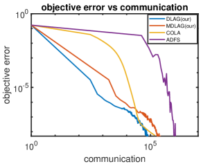
Figure 4: Communication complexities on covtype dataset.

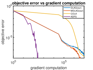
Figure 5: Stochastic gradient complexities on covtype dataset.

From Figures 4 and 5 we can see that ADFS needs more communication than DLAG and MDLAG, as it is not designed to optimize communication complexity. However, ADFS has a better stochastic gradient complexity. This is because at each iteration, ADFS solves a 1-D subproblem that is much simpler than the subproblem (7) of DLAG and MDLAG, this 1-D subproblem is solved approximately by 10 steps of Newton iterations with warm start.

Finally, we would like to emphasize that our algorithms DLAG and MDLAG aim at making SSDA and MSDA practical for problems without cheap dual gradients, and to reduce their communication complexity, while ADFS focuses on optimizing the running time. It is interesting to ask whether our theory for inexact dual gradients can be generalized to provide convergence guarantee for the inexactly solved subproblems in ADFS, where warm start and fixed number of Newton steps are applied.

References

- [1] K. Scaman, F. Bach, S. Bubeck, Y. T. Lee, and L. Massoulié, “Optimal algorithms for smooth and strongly convex distributed optimization in networks,” in Proceedings of the 34th International Conference on Machine Learning-Volume 70. JMLR. org, 2017, pp. 3027–3036.
- [2] W. Shi, Q. Ling, G. Wu, and W. Yin, “Extra: An exact first-order algorithm for decentralized consensus optimization,” SIAM Journal on Optimization, vol. 25, no. 2, pp. 944–966, 2015.
- [3] Y. Nesterov, Introductory Lectures on Convex Optimization: A Basic Course. Springer Science & Business Media, 2013, vol. 87.
- [4] Z. Allen-Zhu, “Katyusha: The first direct acceleration of stochastic gradient methods,” The Journal of Machine Learning Research, vol. 18, no. 1, pp. 8194–8244, 2017.
- [5] T. Chen, G. Giannakis, T. Sun, and W. Yin, “Lag: Lazily aggregated gradient for communication-efficient distributed learning,” in Advances in Neural Information Processing Systems, 2018, pp. 5050–5060.
- [6] J. F. Mota, J. M. Xavier, P. M. Aguiar, and M. Püschel, “D-admm: A communication-efficient distributed algorithm for separable optimization,” IEEE Transactions on Signal Processing, vol. 61, no. 10, pp. 2718–2723, 2013.
- [7] W. Shi, Q. Ling, K. Yuan, G. Wu, and W. Yin, “On the linear convergence of the admm in decentralized consensus optimization,” IEEE Transactions on Signal Processing, vol. 62, no. 7, pp. 1750–1761, 2014.
- [8] K. Yuan, B. Ying, X. Zhao, and A. H. Sayed, “Exact diffusion for distributed optimization and learning—part i: Algorithm development,” IEEE Transactions on Signal Processing, vol. 67, no. 3, pp. 708–723, 2018.
- [9] A. Nedic, A. Olshevsky, and W. Shi, “Achieving geometric convergence for distributed optimization over time-varying graphs,” SIAM Journal on Optimization, vol. 27, no. 4, pp. 2597–2633, 2017.
- [10] L. He, A. Bian, and M. Jaggi, “Cola: Decentralized linear learning,” in Advances in Neural Information Processing Systems, 2018, pp. 4536–4546.
- [11] C. A. Uribe, S. Lee, A. Gasnikov, and A. Nedić, “A dual approach for optimal algorithms in distributed optimization over networks,” arXiv preprint arXiv:1809.00710, 2018.
- [12] H. Sun and M. Hong, “Distributed non-convex first-order optimization and information processing: Lower complexity bounds and rate optimal algorithms,” IEEE Transactions on Signal processing, vol. 67, no. 22, pp. 5912–5928, 2019.
- [13] H. Hendrikx, F. Bach, and L. Massoulie, “An accelerated decentralized stochastic proximal algorithm for finite sums,” arXiv preprint arXiv:1905.11394, 2019.
- [14] A. Koloskova, S. Stich, and M. Jaggi, “Decentralized stochastic optimization and gossip algorithms with compressed communication,” in International Conference on Machine Learning, 2019, pp. 3478–3487.
- [15] A. Mokhtari and A. Ribeiro, “Dsa: Decentralized double stochastic averaging gradient algorithm,” The Journal of Machine Learning Research, vol. 17, no. 1, pp. 2165–2199, 2016.
- [16] Z. Shen, A. Mokhtari, T. Zhou, P. Zhao, and H. Qian, “Towards more efficient stochastic decentralized learning: Faster convergence and sparse communication,” in International Conference on Machine Learning, 2018, pp. 4631–4640.
- [17] H. Sun, S. Lu, and M. Hong, “Improving the sample and communication complexity for decentralized non-convex optimization: A joint gradient estimation and tracking approach,” arXiv preprint arXiv:1910.05857, 2019.
- [18] F. Seide, H. Fu, J. Droppo, G. Li, and D. Yu, “1-bit stochastic gradient descent and its application to data-parallel distributed training of speech dnns,” in Fifteenth Annual Conference of the International Speech Communication Association, 2014.
- [19] N. Strom, “Scalable distributed dnn training using commodity gpu cloud computing,” in Sixteenth Annual Conference of the International Speech Communication Association, 2015.
- [20] D. Alistarh, D. Grubic, J. Li, R. Tomioka, and M. Vojnovic, “Qsgd: Communication-efficient sgd via gradient quantization and encoding,” in Advances in Neural Information Processing Systems, 2017, pp. 1709–1720.
- [21] J. Bernstein, Y.-X. Wang, K. Azizzadenesheli, and A. Anandkumar, “Signsgd: Compressed optimisation for non-convex problems,” in International Conference on Machine Learning, 2018, pp. 559–568.
- [22] S. U. Stich, J.-B. Cordonnier, and M. Jaggi, “Sparsified sgd with memory,” in Advances in Neural Information Processing Systems, 2018, pp. 4447–4458.
- [23] D. Alistarh, T. Hoefler, M. Johansson, N. Konstantinov, S. Khirirat, and C. Renggli, “The convergence of sparsified gradient methods,” in Advances in Neural Information Processing Systems, 2018, pp. 5973–5983.
- [24] J. Wangni, J. Wang, J. Liu, and T. Zhang, “Gradient sparsification for communication-efficient distributed optimization,” in Advances in Neural Information Processing Systems, 2018, pp. 1299–1309.
- [25] T. Lin, S. U. Stich, K. K. Patel, and M. Jaggi, “Don’t use large mini-batches, use local sgd,” arXiv preprint arXiv:1808.07217, 2018.
- [26] S. U. Stich, “Local sgd converges fast and communicates little,” in ICLR 2019 ICLR 2019 International Conference on Learning Representations, no. CONF, 2019.
- [27] H. Yu, S. Yang, and S. Zhu, “Parallel restarted sgd for non-convex optimization with faster convergence and less communication,” arXiv preprint arXiv:1807.06629, 2018.
- [28] J. Wang and G. Joshi, “Cooperative sgd: A unified framework for the design and analysis of communication-efficient sgd algorithms,” arXiv preprint arXiv:1808.07576, 2018.
- [29] A. H. Sayed et al., “Adaptation, learning, and optimization over networks,” Foundations and Trends® in Machine Learning, vol. 7, no. 4-5, pp. 311–801, 2014.
- [30] R. Johnson and T. Zhang, “Accelerating stochastic gradient descent using predictive variance reduction,” in Advances in neural information processing systems, 2013, pp. 315–323.
- [31] H. Hendrikx, L. Massoulié, and F. Bach, “Accelerated decentralized optimization with local updates for smooth and strongly convex objectives,” arXiv preprint arXiv:1810.02660, 2018.
- [32] D. M. Young, Iterative solution of large linear systems. Elsevier, 2014.
- [33] A. C. Wilson, B. Recht, and M. I. Jordan, “A lyapunov analysis of momentum methods in optimization,” arXiv preprint arXiv:1611.02635, 2016.