Convex and Nonconvex Optimization Are Both Minimax-Optimal for Noisy Blind Deconvolution under Random Designs

Abstract

We investigate the effectiveness of convex relaxation and nonconvex optimization in solving bilinear systems of equations under two different designs (i.e. a sort of random Fourier design and Gaussian design). Despite the wide applicability, the theoretical understanding about these two paradigms remains largely inadequate in the presence of random noise. The current paper makes two contributions by demonstrating that: (1) a two-stage nonconvex algorithm attains minimax-optimal accuracy within a logarithmic number of iterations. (2) convex relaxation also achieves minimax-optimal statistical accuracy vis-à-vis random noise. Both results significantly improve upon the state-of-the-art theoretical guarantees.

Keywords: blind deconvolution, bilinear systems of equations, nonconvex optimization, convex relaxation, leave-one-out analysis

1 Introduction and motivation

Suppose we are interested in a pair of unknown objects $\bm{h}^{\star},\bm{x}^{\star}\in\mathbb{C}^{K}$ and are given a collection of $m$ nonlinear measurements taking the following form

$$y_{j}=\bm{b}_{j}^{\mathsf{H}}\bm{h}^{\star}\bm{x}^{\star\mathsf{H}}\bm{a}_{j}+\xi_{j},\qquad 1\leq j\leq m.$$ (1.1)

Here, $\bm{z}^{\mathsf{H}}$ denotes the conjugate transpose of a vector $\bm{z}$, $\left\{\xi_{j}\right\}$ stands for the additive noise, whereas $\left\{\bm{a}_{j}\right\}$ and $\left\{\bm{b}_{j}\right\}$ are design vectors (or sampling vectors). The aim is to faithfully reconstruct both $\bm{h}^{\star}$ and $\bm{x}^{\star}$ from the above set of bilinear measurements.

This problem of solving bilinear systems of equations spans multiple domains in science and engineering, including but not limited to astronomy, medical imaging, optics, and communication engineering (Campisi and Egiazarian, 2016; Jefferies and Christou, 1993; Wang and Poor, 1998; Wunder et al., 2015; Tong et al., 1994; Chan and Wong, 1998). Particularly worth emphasizing is the application of blind deconvolution (Ahmed et al., 2013; Kundur and Hatzinakos, 1996; Ling and Strohmer, 2015; Ma et al., 2018), which involves recovering two unknown signals from their circular convolution. As has been made apparent in the seminal work Ahmed et al. (2013), deconvolving two signals can be reduced to solving bilinear equations, provided that the unknown signals lie within some a priori known subspaces; the interested reader is referred to Ahmed et al. (2013) for details. A variety of approaches have since been put forward for blind deconvolution, most notable of which are convex relaxation and nonconvex optimization (Ahmed et al., 2013; Ling and Strohmer, 2017; Li et al., 2019; Ma et al., 2018; Huang and Hand, 2018; Ling and Strohmer, 2019). Despite a large body of prior work tackling this problem, however, where these algorithms stand vis-à-vis random noise remains unsettled, which we seek to address in the current paper.

1.1 Convex and nonconvex algorithms

Among various algorithms that have been proposed for blind deconvolution, two paradigms have received much attention: (1) convex relaxation and (2) nonconvex optimization, both of which can be explained rather simply. The starting point for both paradigms is a natural least-squares formulation

$$\underset{\bm{h},\bm{x}\in\mathbb{C}^{K}}{\text{minimize}}\quad\sum_{j=1}^{m}\left|\bm{b}_{j}^{\mathsf{H}}\bm{hx}^{\mathsf{H}}\bm{a}_{j}-y_{j}\right|^{2},$$ (1.2)

which is, unfortunately, highly nonconvex due to the bilinear structure of the sampling mechanism. It then boils down to how to guarantee a reliable solution despite the intrinsic nonconvexity.

Convex relaxation.

In order to tame nonconvexity, a popular strategy is to lift the problem into higher dimension followed by convex relaxation (namely, representing $\bm{hx}^{\mathsf{H}}$ by a matrix variable $\bm{Z}$ and then dropping the rank-1 constraint) (Ahmed et al., 2013; Ling and Strohmer, 2015, 2017). More concretely, we consider the following convex program:

$$\underset{\bm{Z}\in\mathbb{C}^{K\times K}}{\mathrm{minimize}}\quad g\left(\bm{Z}\right)=\sum_{j=1}^{m}\left|\bm{b}_{j}^{\mathsf{H}}\bm{Z}\bm{a}_{j}-y_{j}\right|^{2}+2\lambda\left\|\bm{Z}\right\|_{*},$$ (1.3)

where $\lambda>0$ denotes the regularization parameter, and $\|\bm{Z}\|_{*}$ is the nuclear norm of $\bm{Z}$ (i.e.  the sum of singular values of $\bm{Z}$) and is known to be the convex surrogate for the rank function. The rationale is rather simple: given that we seek to recover a rank-1 matrix $\bm{Z}^{\star}=\bm{h}^{\star}\bm{x}^{\star\mathsf{H}}$, it is common to enforce nuclear norm penalization to encourage the rank-1 structure. In truth, this comes down to solving a nuclear-norm regularized least squares problem in the matrix domain $\mathbb{C}^{K\times K}$.

Nonconvex optimization.

Another popular paradigm maintains all iterates in the original vector space (i.e. $\mathbb{C}^{K}$) and attempts solving the above nonconvex formulation or its variants directly. The crucial ingredient is to ensure fast and reliable convergence in spite of nonconvexity. While multiple variants of the nonconvex formulation (1.2) have been studied in the literature (e.g. Li et al. (2019); Ma et al. (2018); Charisopoulos et al. (2019, 2021); Huang and Hand (2018)), the present paper focuses attention on the following ridge-regularized least-squares problem:

$$\underset{\bm{h},\bm{x}\in\mathbb{C}^{K}}{\text{minimize}}\quad f\left(\bm{h},\bm{x}\right) =\sum_{j=1}^{m}\left|\bm{b}_{j}^{\mathsf{H}}\bm{hx}^{\mathsf{H}}\bm{a}_{j}-y_{j}\right|^{2}+\lambda\left\|\bm{h}\right\|_{2}^{2}+\lambda\left\|\bm{x}\right\|_{2}^{2},$$ (1.4)

with $\lambda>0$ the regularization parameter. This choice of objective function is crucial to the establishment of our main theorems as can be seen later. Owing to the nonconvexity of (1.4), one needs to also specify which algorithm to employ in attempt to solve this nonconvex problem. Our focal point is a two-stage optimization algorithm: it starts with a rough initial guess $(\bm{h}^{0},\bm{x}^{0})$ computed by means of a spectral method, followed by Wirtinger gradient descent (GD) that iteratively refines the estimates (to be made precise in (1.6g)). At the end of each gradient iteration, we further rescale the sizes of the two iterates $\bm{h}^{t}$ and $\bm{x}^{t}$, so as to ensure that they have identical $\ell_{2}$ norm (see (1.6l)). In truth, this balancing step helps stabilize the algorithm, while facilitating analysis. The whole algorithm is summarized in Algorithm 1.

Algorithm 1 Nonconvex gradient descent with spectral initialization

  Input: $\left\{y_{j}\right\}_{1\leq j\leq m}$, $\left\{\bm{a}_{j}\right\}_{1\leq j\leq m}$ and $\left\{\bm{b}_{j}\right\}_{1\leq j\leq m}$.

  Spectral initialization: let $\sigma_{1}\left(\bm{M}\right)$, $\check{\bm{h}}^{0}$ and $\check{\bm{x}}^{0}$ denote respectively the leading singular value, the leading left and the right singular vectors of

$$\bm{M}\coloneqq\sum_{j=1}^{m}y_{j}\bm{b}_{j}\bm{a}_{j}^{\mathsf{H}}.$$ (1.5)

Set $\bm{h}^{0}=\sqrt{\sigma_{1}\left(\bm{M}\right)}\,\check{\bm{h}}^{0}$ and $\bm{x}^{0}=\sqrt{\sigma_{1}\left(\bm{M}\right)}\,\check{\bm{x}}^{0}$.

  Gradient updates: for $t=0,1,\ldots,t_{0}-1$ do

  

$$\left[\begin{array}[]{c}\bm{h}^{t+1/2}\\ \bm{x}^{t+1/2}\end{array}\right]= \left[\begin{array}[]{c}\bm{h}^{t}\\ \bm{x}^{t}\end{array}\right]-\eta\left[\begin{array}[]{c}\nabla_{\bm{h}}f\left(\bm{h}^{t},\bm{x}^{t}\right)\\ \nabla_{\bm{x}}f\left(\bm{h}^{t},\bm{x}^{t}\right)\end{array}\right],$$ (1.6g)

$$\left[\begin{array}[]{c}\bm{h}^{t+1}\\ \bm{x}^{t+1}\end{array}\right]= \left[\begin{array}[]{c}\sqrt{\frac{\left\|\bm{x}^{t+1/2}\right\|_{2}}{\left\|\bm{h}^{t+1/2}\right\|_{2}}}\bm{h}^{t+1/2}\\ \sqrt{\frac{\left\|\bm{h}^{t+1/2}\right\|_{2}}{\left\|\bm{x}^{t+1/2}\right\|_{2}}}\bm{x}^{t+1/2}\end{array}\right],$$ (1.6l)

where $\nabla_{\bm{h}}f(\cdot)$ and $\nabla_{\bm{x}}f(\cdot)$ represent the Wirtinger gradient (see Li et al. (2019, Section 3.3) and Appendix A.2.1) of $f(\cdot)$ w.r.t. $\bm{h}$ and $\bm{x}$, respectively.

Table 1: Comparison of our theoretical guarantees of blind deconvolution under Fourier design to prior theory, where we hide all logarithmic factors. Here, the Euclidean estimation error refers to $\|\bm{Z}_{\mathsf{cvx}}-\bm{h}^{\star}\bm{x}^{\star\mathsf{H}}\|_{\mathrm{F}}$ for the convex case and $\|\bm{h}_{\mathsf{ncvx}}\bm{x}_{\mathsf{ncvx}}^{\mathsf{H}}-\bm{h}^{\star}\bm{x}^{\star\mathsf{H}}\|_{\mathrm{F}}$ for the nonconvex case, respectively.

	Sample	Algorithm	Euclidean error	Computational
	complexity		in the noisy case	complexity
Ahmed et al. (2013)	$\mu^{2}K$	convex relaxation	$\sigma\sqrt{Km}$$\frac{1^{7^{7^{7}}}}{1^{7^{7^{7}}}}$	—
Ling and Strohmer (2017)	$\mu^{2}K$	convex relaxation	$\sigma\sqrt{Km}$$\frac{1^{7^{7^{7}}}}{1^{7^{7^{7}}}}$	—
This paper	$\mu^{2}K\vphantom{2_{2_{2_{2}}}^{2^{2^{2}}}}$	convex relaxation	$\sigma\sqrt{K}$$\frac{1^{7^{7^{7}}}}{1^{7^{7^{7}}}}$	—
Li et al. (2019)	$\mu^{2}K\vphantom{2_{2_{2_{2}}}^{2^{2^{2}}}}$	nonconvex regularized GD	$\sigma\sqrt{K}$$\frac{1^{7^{7^{7}}}}{1^{7^{7^{7}}}}$	$mK^{2}$
Huang and Hand (2018)	$\mu^{2}K\vphantom{2_{2_{2_{2}}}^{2^{2^{2}}}}$	Riemannian steepest descent	$\sigma\sqrt{K}$$\frac{1^{7^{7^{7}}}}{1^{7^{7^{7}}}}$	$mK^{2}$
Ma et al. (2018)	$\mu^{2}K\vphantom{2_{2_{2_{2}}}^{2^{2^{2}}}}$	nonconvex vanilla GD	—	$mK$ (noiseless)
This paper	$\mu^{2}K\vphantom{2_{2_{2_{2}}}^{2^{2^{2}}}}$	nonconvex GD	$\sigma\sqrt{K}$$\frac{1^{7^{7^{7}}}}{1^{7^{7^{7}}}}$	$mK$
		(with balancing operations)

1.2 Inadequacy of prior theory

The aforementioned two algorithms have found solid theoretical support under certain randomized sampling mechanisms. Informally, imagine that the $\bm{a}_{j}$’s and the $\bm{b}_{j}$’s follow standard Gaussian and partial Fourier designs, respectively, and that each noise component $\xi_{j}$ is a zero-mean sub-Gaussian random variable with variance at most $\sigma^{2}$ (more precise descriptions are deferred to Assumption 1). The following performance guarantees have been established in prior theory.

• Convex relaxation is guaranteed to return an estimate of $\bm{h}^{\star}\bm{x}^{\star\mathsf{H}}$ with an Euclidean estimation error bounded by $\sigma\sqrt{Km}$ (modulo some log factor) (Ahmed et al., 2013; Ling and Strohmer, 2017). This, however, exceeds the minimax lower bound (to be presented in Theorem 5) by at least a factor of $\sqrt{m}$.

• In comparison, nonconvex algorithms are capable of achieving nearly minimax optimal statistical accuracy, with a computational complexity on the order of $mK^{2}$ (up to some log factor) (Li et al., 2019; Huang and Hand, 2018). Here, the computational complexity encompasses the cost of spectral initialization in Algorithm 1 if implemented by power methods (Golub and Van Loan, 2013). This computational cost, however, could be an order of $K$ times larger than the cost taken to read the data.

See Table 1 for a more complete summary of existing theoretical results for this scenario.

These prior results, while offering rigorous theoretical underpinnings for the two popular algorithms, lead to several natural questions:

1. (Improving statistical guarantees) Is the statistical accuracy of convex relaxation inherently suboptimal when coping with random noise?

2. (Improving computational complexity) Is it possible to further accelerate the nonconvex algorithm without compromising statistical accuracy?

The present paper is devoted to addressing these two questions. Informally, we aim to demonstrate that (1) convex relaxation achieves minimax-optimal statistical accuracy in the face of random noise, and (2) nonconvex optimization converges to a nearly minimax-optimal solution in time proportional to that taken to read the data.

1.3 Paper organization and notation

The outline of the paper is as follows. Section 2 gives the formal statement of the model assumptions and presents our main results for two different designs. Section 3 reviews previous literature on blind deconvolution. Section 4 presents numerical experiments that corroborate our theoretical results. We conclude the paper in Section 5 by pointing out several future directions. All the proof details are deferred to the Appendix.

Throughout the paper, we shall often use the vector notation $\bm{y}:=[y_{1},\cdots,y_{m}]^{\top}$ and $\bm{\xi}:=[\xi_{1},\cdots,\xi_{m}]^{\top}\in\mathbb{C}^{m}$. For any vector $\bm{v}$ and any matrix $\bm{M}$, we denote by $\bm{v}^{\mathsf{H}}$ and $\bm{M}^{\mathsf{H}}$ their conjugate transpose, respectively. The notation $\|\bm{v}\|_{2}$ represents the $\ell_{2}$ norm of an vector $\bm{v}$, and we let $\left\|\bm{M}\right\|$, $\left\|\bm{M}\right\|_{\mathrm{F}}$ and $\left\|\bm{M}\right\|_{*}$ represent the spectral norm, the Frobenius norm and the nuclear norm of $\bm{M}$, respectively. For a function $f(\bm{h},\bm{x})$, we use $\nabla_{\bm{h}}f(\bm{h},\bm{x})$ (resp. $\nabla_{\bm{x}}f(\bm{h},\bm{x})$) to denote its Wirtinger gradient (see Li et al. (2019, Section 3.3) for detailed introduction) of $f(\cdot)$ with respect to $\bm{h}$ (resp. $\bm{x}$). Further, we define $\nabla f(\bm{h},\bm{x})=[\nabla_{\bm{h}}f(\bm{h},\bm{x})^{\top},\nabla_{\bm{x}}f(\bm{h},\bm{x})^{\top}]^{\top}$. For any subspace $T$, we use $T^{\bot}$ to denote its orthogonal complement, and $\mathcal{P}_{T}(\bm{M})$ the Euclidean projection of a matrix $\bm{M}$ onto $T$. Moreover, we adopt $f_{1}(m,K)\lesssim f_{2}(m,K)$ or $f_{1}(m,K)=O(f_{2}(m,K))$ to indicate that there exists some constant $C_{1}>0$ such that $f_{1}(m,K)\leq Cf_{2}(m,K)$ holds for all $(m,K)$ that are sufficiently large, and use $f_{1}(m,K)\gtrsim f_{2}(m,K)$ to indicate that $f_{1}(m,K)\geq C_{2}f_{2}(m,K)$ holds for some constant $C>0$ whenever $(m,K)$ are sufficiently large. The notation $f_{1}(m,K)\asymp f_{2}(m,K)$ means that $f_{1}(m,K)\lesssim f_{2}(m,K)$ and $f_{1}(m,K)\gtrsim f_{2}(m,K)$ hold simultaneously. In our proof, $C$ serves as a universal constant whose value might change from line to line.

2 Main results

In this section, we present our theoretical guarantees for the above two algorithms for two types of random designs commonly studied in the blind deconvolution literature.

2.1 Blind deconvolution under random Fourier designs

Model and assumptions.

We start by introducing a sort of random Fourier designs motivated by practical engineering applications (see Ahmed et al. (2013); Li et al. (2019)).

Assumption 1.

Let $\bm{A}:=\left[\bm{a}_{1},\bm{a}_{2},\cdots,\bm{a}_{m}\right]^{\mathsf{H}}\in\mathbb{C}^{m\times K}$ and $\bm{B}:=\left[\bm{b}_{1},\bm{b}_{2},\cdots,\bm{b}_{m}\right]^{\mathsf{H}}\in\mathbb{C}^{m\times K}$ be matrices obtained by concatenating the design vectors.

• The entries of $\bm{A}$ are independently drawn from standard complex Gaussian distributions, namely, $\bm{a}_{j}\overset{\mathrm{i.i.d.}}{\sim}\mathcal{N}\left(\bm{0},\frac{1}{2}\bm{I}_{K}\right)+i\mathcal{N}\left(\bm{0},\frac{1}{2}\bm{I}_{K}\right)$ with $i$ the imaginary unit;

• The design matrix $\bm{B}$ consists of the first $K$ columns of the unitary discrete Fourier transform (DFT) matrix $\bm{F}\in\mathbb{C}^{m\times m}$ obeying $\bm{F}\bm{F}^{\mathsf{H}}=\bm{I}_{m}$;

• The noise components $\{\xi_{i}\}$ are independent zero-mean sub-Gaussian random variables with sub-Gaussian norm obeying $\|\xi_{i}\|_{\psi_{2}}\leq\sigma$ ($1\leq i\leq m)$. See Vershynin (2010, Definition 5.7) for the definition of $\|\cdot\|_{\psi_{2}}$.

Remark 1.

As can be easily verified, we have $\left\|\bm{b}_{j}\right\|_{2}=\sqrt{K/m}$ ($1\leq j\leq m$) under this model.

It is worth noting that the Fourier design is largely motivated by the duality relation between convolution in the time domain and multiplication in the frequency domain, which is closely related to practical scenarios; see Ahmed et al. (2013) for details. In fact, the model described in Assumption 1 has been the focus of a number of recent papers including Ahmed et al. (2013); Li et al. (2019); Ma et al. (2018); Huang and Hand (2018); Ling and Strohmer (2019, 2016, 2017), to name a few.

In addition, as pointed out by prior works Ahmed et al. (2013); Li et al. (2019); Ma et al. (2018), the following incoherence condition — which captures the interplay between the truth and the measurement mechanism — plays a crucial role in enabling tractable estimation schemes.

Definition 1 (Incoherence).

Define the incoherence parameter $\mu$ as the smallest number obeying

$$\left|\bm{b}_{j}^{\mathsf{H}}\bm{h}^{\star}\right|\leq\frac{\mu}{\sqrt{K}}\left\|\bm{b}_{j}\right\|_{2}\left\|\bm{h}^{\star}\right\|_{2}=\frac{\mu}{\sqrt{m}}\left\|\bm{h}^{\star}\right\|_{2},\qquad 1\leq j\leq m.$$ (2.1)

Remark 2.

Comparing the Cauchy-Schwarz inequality $\left|\bm{b}_{j}^{\mathsf{H}}\bm{h}^{\star}\right|\leq\left\|\bm{b}_{j}\right\|_{2}\left\|\bm{h}^{\star}\right\|_{2}$ with (2.1) reveals that $\mu\leq\sqrt{K}$. It is noteworthy that our theory does not require $\mu$ to be small constant; in fact, all of our theoretical findings allow $\mu$ to grow with the problem dimension.

Informally, a small incoherence parameter indicates that the truth is not quite aligned with the sampling basis. As a concrete example, when $\bm{h}^{\star}$ is randomly generated (i.e. $\bm{h}^{\star}\sim\mathcal{N}(\bm{0},\bm{I}_{K})$), it can be easily verified that the incoherence parameter $\mu$ is, with high probability, at most $O(\sqrt{\log m})$. In fact, this type of condition is widely proposed in statistical literature on various problem besides blind deconvolution, such as Candès and Recht (2009); Ma et al. (2018); Chen et al. (2020b) on matrix completion and Candès et al. (2011); Chandrasekaran et al. (2011); Chen et al. (2020c) on robust principal component analysis. The important role of this incoherence parameter will also be confirmed by our numerical simulations momentarily (cf. Figure 3).

Main theory.

We are now positioned to state our main theory for this setting, followed by discussing the implications of our theory. Towards this end, we begin with the statistical guarantees for the convex formulation. Denote the minimizer of (1.3) by $\bm{Z}_{\mathsf{cvx}}$. Then our result is this:

Theorem 1 (Convex relaxation).

Set $\lambda=C_{\lambda}\sigma\sqrt{K\log m}$ for some large enough constant $C_{\lambda}>0$. Assume

$$m\geq C\mu^{2}K\log^{9}m\qquad\text{and}\qquad\sigma\sqrt{K\log^{5}m}\leq c\left\|\bm{h}^{\star}\bm{x}^{\mathsf{\star H}}\right\|_{\mathrm{F}}$$ (2.2)

for some sufficiently large (resp. small) constant $C>0$ (resp. $c>0$). Then under Assumption 1 and the incoherence condition (2.1), one has with probability exceeding $1-O\left(m^{-3}+me^{-K}\right)$ that

$$\left\|\bm{Z}_{\mathsf{cvx}}-\bm{h}^{\star}\bm{x}^{\mathsf{\star H}}\right\|\leq\left\|\bm{Z}_{\mathsf{cvx}}-\bm{h}^{\star}\bm{x}^{\mathsf{\star H}}\right\|_{\mathrm{F}} \lesssim\sigma\sqrt{K\log m}.$$ (2.3)

In addition, the bounds in (2.3) continue to hold if $\bm{Z}_{\mathsf{cvx}}$ is replaced by $\bm{Z}_{\mathsf{cvx,}1}\coloneqq\arg\min_{\bm{Z}:\mathsf{rank}\left(\bm{Z}\right)\leq 1}\left\|\bm{Z}-\bm{Z}_{\mathsf{cvx}}\right\|_{\mathrm{F}}$ (i.e. the best rank-1 approximation of $\bm{Z}_{\mathsf{cvx}}$).

Remark 3.

In (2.2), $\log^{9}m$ and $\log^{5}m$ appear due to our decoupling arguments. We believe it would be difficult to get rid of the logarithmic factors completely using the current analyis framework, although it might be possible to reduce the power of the logarithmic factors slightly by means of more refined analysis.

Our proof for this theorem, whose details are postponed to Appendix B.1, is largely inspired by the idea of connecting convex and nonconvecx optimization as proposed by Chen et al. (2020b, c) for noisy matrix completion and robust principal component analysis respectively. Note, however, that implementing this high-level idea requires drastically different analysis from Chen et al. (2020b, c), primarily due to the absence of randomness in the highly structured Fourier design matrix $\bm{B}$. For instance, in contrast to prior works that were built upon a “leave-one-out” analysis framework to decouple statistical dependency, simply “leaving out” one row of $\bm{B}$ in the blind deconvolution analysis does not lead to immediate statistical benefits due to the deterministic nature of $\bm{B}$. Consequently, considerably more delicate analyses are needed in order to enable fine-grained statistical analysis.

Next, we turn to theoretical guarantees for the nonconvex algorithm described in Algorithm 1. For notational convenience, we define

$$\bm{z}^{t}:=\left[\begin{array}[]{c}\bm{h}^{t}\\ \bm{x}^{t}\end{array}\right]\qquad\text{and}\qquad\bm{z}^{\star}:=\left[\begin{array}[]{c}\bm{h}^{\star}\\ \bm{x}^{\star}\end{array}\right]$$ (2.4)

throughout this paper. Before presenting the results, we make note of an unavoidable scaling ambiguity issue underlying this model. Given that $\bm{h}^{\star}$ and $\bm{x}^{\star}$ are only identifiable up to global scaling (meaning that one cannot hope to distinguish $(\alpha\bm{h}^{\star},\frac{1}{\overline{\alpha}}\bm{x}^{\star})$ from $(\bm{h}^{\star},\bm{x}^{\star})$ given only bilinear measurements), we shall measure the discrepancy between $\bm{z}^{\star}$ and any point $\bm{z}:=\footnotesize\left[\begin{array}[]{c}\bm{h}\\ \bm{x}\end{array}\right]$ through the following metric:

$$\mathsf{dist}\left(\bm{z},\bm{z}^{\star}\right):=\min_{\alpha\in\mathbb{C}}\sqrt{\left\|\frac{1}{\overline{\alpha}}\bm{h}-\bm{h}^{\star}\right\|_{2}^{2}+\left\|\alpha\bm{x}-\bm{x}^{\star}\right\|_{2}^{2}}.$$ (2.5)

In words, this metric is an extension of the $\ell_{2}$ distance modulo global scaling. Our result is this:

Theorem 2 (Nonconvex optimization).

Set $\lambda=C_{\lambda}\sigma\sqrt{K\log m}$ for some large enough constant $C_{\lambda}>0$. Take $\eta=c_{\eta}$ for some sufficiently small constant $c_{\eta}>0$. Suppose that Assumption 1, the incoherence condition (2.1) and the condition (2.2) hold. Then with probability at least $1-O\left(m^{-5}+me^{-K}\right)$, the iterates $\left\{\bm{h}^{t},\bm{x}^{t}\right\}_{0\leq t\leq t_{0}}$ of the spectrally initialized nonconvex algorithm (see Algorithm 1) obey

$$\mathsf{dist}\left(\bm{z}^{0},\bm{z}^{\star}\right) \lesssim\sqrt{\frac{\mu^{2}K\log m}{m}}\left\|\bm{z}^{\star}\right\|_{2}+\frac{\sigma\sqrt{K\log m}}{\left\|\bm{h}^{\star}\bm{x}^{\mathsf{\star H}}\right\|_{\mathrm{F}}^{1/2}},$$ (2.6a)

$$\mathsf{dist}\left(\bm{z}^{t},\bm{z}^{\star}\right) \leq\rho^{t}\mathsf{dist}\left(\bm{z}^{0},\bm{z}^{\star}\right)+\frac{C_{1}\left(\lambda+\sigma\sqrt{K\log m}\right)}{c_{\rho}\left\|\bm{h}^{\star}\bm{x}^{\mathsf{\star H}}\right\|_{\mathrm{F}}^{1/2}},$$ (2.6b)

$$\big{\|}\bm{h}^{t}\big{(}\bm{x}^{t}\big{)}^{\mathsf{H}}-\bm{h}^{\star}\bm{x}^{\mathsf{\star H}}\big{\|}_{\mathrm{F}} \leq 2\rho^{t}\mathsf{dist}\left(\bm{z}^{0},\bm{z}^{\star}\right)\left\|\bm{z}^{\star}\right\|_{2}+\frac{2C_{1}\left(\lambda+\sigma\sqrt{K\log m}\right)}{c_{\rho}},$$ (2.6c)

simultaneously for all $0\leq t\leq t_{0}\leq m^{20}$. Here, we take $C_{1}>0$ to be some sufficiently large constant and $0<\rho=1-c_{\rho}\eta<1$ for some sufficiently small constant $c_{\rho}>0$.

Remark 4.

It is noteworthy that the quantity $m^{-5}$ in the probability term $1-O\left(m^{-5}+me^{-K}\right)$ in this theorem can actually be replaced by $m^{-C}$ for any positive integer $C$.

Informally, this theorem guarantees that the estimation error of the iterates $\left\{\bm{h}^{t},\bm{x}^{t}\right\}_{0\leq t\leq t_{0}}$ generated by Algorithm 1 decays geometrically fast until some error floor is hit. As we shall demonstrate momentarily in Theorem 5, this error floor matches the minimax-optimal statistical error up to some logarithmic term.

Compared with one of the most relevant papers to us — Ma et al. (2018) — on blind deconvolution under Fourier designs, this theorem generalizes the noiseless case studied in Ma et al. (2018) to the noisy case. This generalization actually needs a lot of efforts since it calls for delicate and careful control of the noise effect, as detailed in the proof in Appendix A.

2.2 Blind deconvolution under Gaussian designs

In addition to the above-mentioned random Fourier design, our results also extend to the scenario under Gaussian design, as formalized below.

Model and assumptions.

Let us describe the model and assumptions of this scenario as follows.

Assumption 2.

Let $\bm{A}:=\left[\bm{a}_{1},\bm{a}_{2},\cdots,\bm{a}_{m}\right]^{\mathsf{H}}\in\mathbb{C}^{m\times K}$ and $\bm{B}:=\left[\bm{b}_{1},\bm{b}_{2},\cdots,\bm{b}_{m}\right]^{\mathsf{H}}\in\mathbb{C}^{m\times K}$ be matrices obtained by concatenating the design vectors.

• The entries of $\bm{A}$ and $\bm{B}$ are independently drawn from standard complex Gaussian distributions, namely, $\bm{a}_{j},\bm{b}_{j}\overset{\mathrm{i.i.d.}}{\sim}\mathcal{N}\left(\bm{0},\frac{1}{2}\bm{I}_{K}\right)+i\mathcal{N}\left(\bm{0},\frac{1}{2}\bm{I}_{K}\right)$ with $i$ the imaginary unit;

• The noise components $\{\xi_{i}\}$ are independent zero-mean sub-Gaussian random variables with sub-Gaussian norm obeying $\|\xi_{i}\|_{\psi_{2}}\leq\sigma$ ($1\leq i\leq m)$. See Vershynin (2010, Definition 5.7) for the definition of $\|\cdot\|_{\psi_{2}}$.

Akin to Theorems 1 and 2, we consider the loss functions (1.3) and (1.4). The main results under the Gaussian design are summarized in the following theorems.

Theorem 3 (Convex relaxation).

Let $\lambda=C_{\lambda}\sigma\sqrt{mK\log m}$ for some sufficiently large constant $C_{\lambda}>0$. Assume the sample complexity and the noise level satisfy

$$m\geq CK\log^{6}m\qquad\text{and}\qquad\sigma\sqrt{\frac{K\log^{5}m}{m}}\leq c\left\|\bm{h}^{\star}\bm{x}^{\mathsf{\star H}}\right\|_{\mathrm{F}}$$ (2.7)

for some sufficiently large (resp. small) constant $C>0$ (resp. $c>0$). Then

$$\left\|\bm{Z}_{\mathsf{cvx}}-\bm{h}^{\star}\bm{x}^{\mathsf{\star H}}\right\|\leq\left\|\bm{Z}_{\mathsf{cvx}}-\bm{h}^{\star}\bm{x}^{\mathsf{\star H}}\right\|_{\mathrm{F}}\lesssim\sigma\sqrt{\frac{K\log m}{m}}$$ (2.8)

holds with probability at least $1-O(m^{-5}+m\exp(-c_{1}K))$ for some constant $c_{1}>0$. In addition, the bounds in (2.8) continue to hold if $\bm{Z}_{\mathsf{cvx}}$ is replaced by $\bm{Z}_{\mathsf{cvx,}1}\coloneqq\arg\min_{\bm{Z}:\mathsf{rank}\left(\bm{Z}\right)\leq 1}\left\|\bm{Z}-\bm{Z}_{\mathsf{cvx}}\right\|_{\mathrm{F}}$ (i.e. the best rank-1 approximation of $\bm{Z}_{\mathsf{cvx}}$).

This theorem, which is in parallel to Theorem 1 for Fourier designs, confirms the appealing statistical guarantees of convex relaxation under Gaussian designs. The minimax optimality of this result will be discussed in Section 2.3 in detail.

Theorem 4 (Nonconvex optimization).

Set $\lambda=C_{\lambda}\sigma\sqrt{mK\log m}$ for some large enough constant $C_{\lambda}>0$. Take $\eta=c_{\eta}/m$ for some sufficiently small constant $c_{\eta}>0$. Suppose that Assumption 2 and Condition (2.7) hold. Then with probability at least $1-O\left(m^{-5}+me^{-K}\right)$, the iterates $\left\{\bm{h}^{t},\bm{x}^{t}\right\}_{0\leq t\leq t_{0}}$ of Algorithm 1 obey

$$\mathsf{dist}\left(\bm{z}^{0},\bm{z}^{\star}\right) \lesssim\sqrt{\frac{K\log^{2}m}{m}}\left\|\bm{z}^{\star}\right\|_{2}+\sigma\sqrt{\frac{K\log m}{m\left\|\bm{h}^{\star}\bm{x}^{\mathsf{\star H}}\right\|_{\mathrm{F}}}},$$ (2.9a)

$$\mathsf{dist}\left(\bm{z}^{t},\bm{z}^{\star}\right) \leq\rho^{t}\mathsf{dist}\left(\bm{z}^{0},\bm{z}^{\star}\right)+\frac{C_{11}\left(\lambda+\sigma\sqrt{mK\log m}\right)}{c_{\rho}m\left\|\bm{h}^{\star}\bm{x}^{\mathsf{\star H}}\right\|_{\mathrm{F}}^{1/2}}$$ (2.9b)

$$\big{\|}\bm{h}^{t}\big{(}\bm{x}^{t}\big{)}^{\mathsf{H}}-\bm{h}^{\star}\bm{x}^{\mathsf{\star H}}\big{\|}_{\mathrm{F}} \leq 2\rho^{t}\mathsf{dist}\left(\bm{z}^{0},\bm{z}^{\star}\right)\left\|\bm{z}^{\star}\right\|_{2}+\frac{2C_{11}\left(\lambda+\sigma\sqrt{mK\log m}\right)}{c_{\rho}m}$$ (2.9c)

simultaneously for all $0\leq t\leq t_{0}\leq m^{20}$. Here, we take $C_{11}>0$ to be some sufficiently large constant and $0<\rho=1-c_{\rho}c_{\eta}<1$ for some sufficiently small constant $c_{\rho}>0$.

Similar to the Fourier designs studied in Section 2.1, our theory asserts that the estimation error of $\left\{\bm{h}^{t},\bm{x}^{t}\right\}_{0\leq t\leq t_{0}}$ produced by Algorithm 1 decreases geometrically fast before reaching an error floor on the order of the minimax-optimal statistical limit modulo some logarithmic factor (cf. Theorem 5).

2.3 Insights

The above theorems strengthen our understanding about the performance of both convex and nonconvex algorithms in the presence of random noise. In what follows, we elaborate on the tightness of our results as well as other important algorithmic implications.

• Minimax optimality of both convex relaxation and nonconvex optimization. Theorems 1-2 (resp. Theorems 3-4) reveal that both convex and nonconvex optimization estimate $\bm{h}^{\star}\bm{x}^{\mathsf{\star H}}$ to within an Euclidean error at most $\sigma\sqrt{K}$ (resp. $\sigma\sqrt{mK}$) up to some log factor for random Fourier design (resp. Gaussian design), provided that the regularization parameter is taken to be $\lambda\asymp\sigma\sqrt{K\log m}$ (resp. $\lambda\asymp\sigma\sqrt{mK\log m}$). This closes the gap between the statistical guarantees for convex and nonconvex optimization, confirming that convex relaxation is no less statistically efficient than nonconvex optimization. Further, in order to assess the statistical optimality of our results, it is instrumental to understand the statistical limit one can hope for. This is provided in the following claim, whose proof is postponed to Appendix E.

  Theorem 5.

  Suppose that the noise components obey $\xi_{j}\overset{\text{i.i.d.}}{\sim}\mathcal{N}(0,\sigma^{2}/2)+i\mathcal{N}(0,\sigma^{2}/2)$. Define

  $$\mathcal{M}^{\star}\coloneqq\left\{\bm{Z}=\bm{h}\bm{x}^{\mathsf{H}}\,\big{|}\,\bm{h},\bm{x}\in\mathbb{C}^{K}\right\}.$$

  Then under Assumption 1, there exists some universal constant $c_{\mathsf{lb}}^{(1)}>0$ such that, with probability exceeding $1-O(K^{-10})$,

  $$\inf_{\widehat{\bm{Z}}}\sup_{\bm{Z}^{\star}\in\mathcal{M}^{\star}}\mathbb{E}\left[\big{\|}\widehat{\bm{Z}}-\bm{Z}^{\star}\big{\|}_{\mathrm{F}}^{2}\mid\bm{A}\right]\geq c_{\mathsf{lb}}^{(1)}\frac{\sigma^{2}K}{\log m},$$ (2.10)

  where the infimum is taken over all estimator $\widehat{\bm{Z}}$. Furthermore, under Assumption 2, there exists another universal constant $c_{\mathsf{lb}}^{(2)}>0$ such that

  $$\inf_{\widehat{\bm{Z}}}\sup_{\bm{Z}^{\star}\in\mathcal{M}^{\star}}\mathbb{E}\left[\big{\|}\widehat{\bm{Z}}-\bm{Z}^{\star}\big{\|}_{\mathrm{F}}^{2}\mid\bm{A},\bm{B}\right]\geq c_{\mathsf{lb}}^{(2)}\frac{\sigma^{2}K}{m\log m}$$ (2.11)

  holds with probability exceeding $1-O(K^{-10})$.

  Encouragingly, the minimax lower bound (2.10) (resp. (2.11)) matches the statistical error bounds in Theorems 1-2 (resp. Theorems 3-4) up to some logarithmic factor, thus confirming the near minimaxity of both convex relaxation and nonconvex optimization for blind deconvolution under both designs.

• Fast convergence of nonconvex algorithms. From the computational perspective, Theorem 2 guarantees linear convergence (or geometric convergence) of the nonconvex algorithm with a contraction rate $\rho$. Given that $1-\rho$ is a constant bounded away from 1 (as long as the stepsize is taken to be a sufficiently small constant), the iteration complexity of the algorithm scales at most logarithmically with the model parameters. As a result, the total computational complexity is proportional to the per-iteration cost $O(mK)$ (up to some log factor), which scales nearly linearly with the time taken to read the data. Compared with past work on nonconvex algorithms (Li et al., 2019; Huang and Hand, 2018), our theory reveals considerably faster convergence and hence improved computational cost, without compromising statistical efficiency. A key enabler of the improved theory lies in fine-grained understanding of the part of optimization lanscape visited by the nonconvex algorithm, thus allowing for the use of more aggressive constant step sizes instead of diminishing step sizes. See Table 1 for details.

The careful reader might immediately remark that the validity of the above results requires the assumptions (2.2) on both the sample size and the noise level. Fortunately, a closer inspection of these conditions reveals the broad applicability of these conditions.

• Sample complexity. The sample size requirement in our theory of blind deconvolution under Fourier design (resp. Gaussian design), as stated in Condition (2.2) (resp. Condition (2.7)), scales as

  $$m\gtrsim K\mathrm{poly}\log(m),$$

  which matches the information-theoretical lower limit even in the absence of noise (modulo some logarithmic factor) as proved in Kech and Krahmer (2017) (resp. Cai et al. (2015)).

• Signal-to-noise ratio (SNR). The noise level required for our theory to work under Fourier design (see Condition (2.2)) is given by $\sigma\sqrt{K\log^{5}m}\lesssim\left\|\bm{h}^{\star}\bm{x}^{\star\mathsf{H}}\right\|_{\mathrm{F}}$. If we define the sample-wise signal-to-noise ratio as follows

  $$\mathsf{SNR}:=\frac{\frac{1}{m}\sum_{k=1}^{m}\mathbb{E}\big{[}\big{|}\bm{b}_{k}^{\mathsf{H}}\bm{h}^{\star}\bm{x}^{\star\mathsf{H}}\bm{a}\big{|}^{2}\big{]}}{\sigma^{2}},$$ (2.12)

  then our noise requirement can be equivalently phrased as

  $$\mathsf{SNR}=\frac{\|\bm{h}^{\star}\|_{2}^{2}\|\bm{x}^{\star}\|_{2}^{2}}{m\sigma^{2}}\gtrsim\frac{K\log^{5}m}{m},$$

  where the right-hand side of the above relation is vanishingly small in light of our sample complexity constraint $m\gtrsim\mu^{2}K\log^{9}m$. In other words, our theory works even in the low-SNR regime. Furthermore, for the Gaussian design, the noise level required in our theory is $\sigma\sqrt{K\log^{5}m/m}\lesssim\left\|\bm{h}^{\star}\bm{x}^{\star\mathsf{H}}\right\|_{\mathrm{F}}$. We can introduce the following SNR that allows us to rewrite this requirement as

  $$\mathsf{SNR}=\frac{\frac{1}{m}\sum_{k=1}^{m}\mathbb{E}\big{[}\big{|}\bm{b}_{k}^{\mathsf{H}}\bm{h}^{\star}\bm{x}^{\star\mathsf{H}}\bm{a}\big{|}^{2}\big{]}}{\sigma^{2}}=\frac{\|\bm{h}^{\star}\|_{2}^{2}\|\bm{x}^{\star}\|_{2}^{2}}{\sigma^{2}}\gtrsim\frac{K\log^{5}m}{m},$$

  which resembles the one for Fourier designs.

3 Prior art

Before embarking on our discussion on the prior art for blind deconvolution, it is noteworthy that the model (1.1) might remind readers of the famous problem of phase retrieval (Candes et al., 2013; Shechtman et al., 2015; Chi et al., 2019), which is concerned with solving random quadratic systems of equations and clearly related to the problem of solving bilinear systems. Despite the similarity between these two problems at first glance, the majority of prior phase retrieval theory focuses on either i.i.d. Gaussian designs or randomized coded diffraction patterns, which are drastically different from the kind of random Fourier designs commonly assumed in blind deconvolution. In fact, the presence of Fourier designs in blind deconvolution is a consequence of the duality relation between convolution in the time domain and multiplication in the frequency domain (Ahmed et al., 2013; Li et al., 2019). The deterministic nature of the Fourier design matrix $\bm{B}$ under the Fourier model, however, presents a substantial challenge in the analysis of both convex and nonconvex optimization algorithms; in contrast, the Gaussian design matrix in prior phase retrieval theory is assumed to be highly random, which remarkably simplifies analysis.

We now turn attention to the blind deconvolution literature. As mentioned previously, recent years have witnessed much progress towards understanding convex and nonconvex optimization for solving bilinear systems of equations. First, we give a brief review on previous literature of blind deconvolution under Fourier design. Regarding the convex programming approach, Ahmed et al. (2013) was the first to apply the lifting idea to transform bilinear system of equations into linear measurements about a rank-one matrix — an idea that has proved effective in a number of nonconvex problems (Candes et al., 2013; Waldspurger et al., 2015; Chen and Chi, 2014; Tang et al., 2013; Chi, 2016; Chen et al., 2014; Goemans and Williamson, 1994; Shechtman et al., 2014; Oymak et al., 2015). Focusing on convex relaxing in the lifted domain, Ahmed et al. (2013) showed that exact recovery is possible from a near-optimal number of measurements in the noiseless case, and developed the first statistical guarantees for the noisy case (which are, as alluded to previously, highly suboptimal). Several other works have also been devoted to understanding convex relaxation under possibly different assumptions. Another paper Aghasi et al. (2019) proposed an effective convex algorithm for bilinear inversion, assuming that the signs of the signals are known a priori. Moving beyond blind deconvolution, the convex approach has been extended to accommodate the blind demixing problem (Ling and Strohmer, 2017; Jung et al., 2017), which is more general than blind deconvolution.

$$\underset{\bm{Z}\in\mathbb{C}^{K\times K}}{\mathrm{minimize}}\quad\left\|\bm{Z}\right\|_{*}\qquad\text{subject\ to}\quad\bm{y}=\mathcal{A}\left(\bm{Z}\right).$$

Another line of works has focused on the development of fast nonconvex algorithms (Li et al., 2019; Lee et al., 2018; Ma et al., 2018; Huang and Hand, 2018; Ling and Strohmer, 2019; Charisopoulos et al., 2019, 2021), which was largely motivated by recent advances in efficient nonconvex optimization for tackling statistical estimation problems (Candes et al., 2015; Chen and Candès, 2017; Charisopoulos et al., 2021; Keshavan et al., 2009; Jain et al., 2013; Zhang et al., 2016; Chen and Wainwright, 2015; Sun and Luo, 2016; Zheng and Lafferty, 2016; Wang et al., 2017a; Cai et al., 2021b; Wang et al., 2017b; Qu et al., 2017; Duchi and Ruan, 2019; Ma et al., 2019) (see Chi et al. (2019) for an overview). Li et al. (2019) proposed a feasible nonconvex recipe by attempting to optimize a regularized squared loss (which includes extra penalty term to promote incoherence), and showed that in conjunction with proper initialization, nonconvex gradient descent converges to the ground truth in the absence of noise. Another work Huang and Hand (2018) proposed a Riemannian steepest descent method by exploiting the quotient structure, which is also guaranteed to work in the noise-free setting with nearly minimal sample complexity. Further, Ling and Strohmer (2019); Dong and Shi (2018) extended the nonconvex paradigm to accommodate the blind demixing problem, which subsumes blind deconvolution a special case.

Going beyond algorithm designs, the past works Li et al. (2016, 2015); Kech and Krahmer (2017) investigated how many samples are needed to ensure the identifiability of blind deconvolution under the subspace model. Furthermore, it is worth noting that another line of recent works Wang and Chi (2016); Lee et al. (2016); Zhang et al. (2017, 2019, 2020); Li and Bresler (2019); Shi and Chi (2021); Qu et al. (2019) studied a different yet fundamentally important model of blind deconvolution, assuming that one of the two signals is sparse instead of lying within a known subspace. These are, however, beyond the scope of the current paper.

In addition, as far as we know, previous works on blind deconvolution under Gaussian design is not as extensive as the case with Fourier designs, the latter of which is closer to practical blind deconvolution applications. Among the most relevant works: Cai et al. (2015) proposed a constrained convex optimization problem under the same setting as Assumption 2 and establishes that the estimation error is bounded by $\sigma\min\{K\sqrt{\log m}/m+\sqrt{K/m},1\}$, which is on the same order (up to logarithmic factors) as our bound in Theorem 3 when $m\gg K\log m$ and matches the minimax optimal estimation error lower bound; Zhong et al. (2015) studied the noiseless case in terms of both convex and nonconvex formulations; Charisopoulos et al. (2019) analyzed the nonsmooth nonconvex formulation of the problem for bilinear measurements with corruption frequency less than $1/2$, and proved that the subgradient algorithms proposed there converges linearly, while the specific prox-linear method converges quadratically albeit with higher per-iteration cost. Compared with these works, our paper studies the unconstrained version of convex relaxation and establishes an estimation error upper bound that nearly matches the minimax lower bound. When it comes to nonconvex formulation, the current paper is, as far as we know, the first to justify the optimality of its estimation accuracy in the noisy setting.

At the technical level, the pivotal idea of our paper lies in bridging convex and nonconvex estimators, which is motivated by prior works Chen et al. (2020b, 2019c, c) on matrix completion and robust principal component analysis. Such crucial connections have been established with the assistance of the leave-one-out analysis framework, which has already proved effective in analyzing a variety of nonconvex statistical problems (El Karoui, 2018; Chen et al., 2019a, b; Ding and Chen, 2020; Cai et al., 2020; Dong and Shi, 2018; Xu et al., 2019; Cai et al., 2021a; Chen et al., 2020a; Zhong and Boumal, 2018).

4 Numerical experiments

In this subsection, we carry out a series of numerical experiments to confirm the validity of our theory. Throughout the experiments, the signals of interest $\bm{h}^{\star}$, $\bm{x}^{\star}\in\mathbb{C}^{K}$ are drawn from $\mathcal{N}\left(\bm{0},\frac{1}{2K}\bm{I}_{K}\right)+\text{i}\mathcal{N}\left(\bm{0},\frac{1}{2K}\bm{I}_{K}\right)$ (so that they have approximately unit $\ell_{2}$ norm). Under the Assumption 1 (resp. Assumption 2), the stepsize $\eta$ is set to be $0.05$ (resp. $0.05/m$), whereas the regularization parameter is taken to be $\lambda=5\sigma\sqrt{K\log m}$ (resp. $\lambda=5\sigma\sqrt{mK\log m}$). The convex problem is solved by means of the proximal gradient method (Parikh and Boyd, 2014).

In the first series of experiments, we report the statistical estimation errors of both convex and nonconvex approaches as the noise level $\sigma$ varies from $10^{-6}$ to $10^{-3}$ for blind deconvolution under Fourier design, while the noise level for blind deconvolution under Gaussian design is from $10^{-5}$ to $10^{-2}$; here, we set $K=100$ and $m=10K$. Let $\bm{Z}_{\mathsf{ncvx}}=\bm{h}_{\mathsf{ncvx}}\bm{x}_{\mathsf{ncvx}}^{\mathsf{H}}$ be the nonconvex solution and $\bm{Z}_{\mathsf{cvx}}$ be the convex solution. Figure 1 depicts the relative Euclidean estimation errors ($\left\|\bm{Z}_{\mathsf{ncvx}}-\bm{Z}^{\star}\right\|_{\text{F}}/\left\|\bm{Z}^{\star}\right\|_{\text{F}}$ and $\left\|\bm{Z}_{\mathsf{cvx}}-\bm{Z}^{\star}\right\|_{\text{F}}/\left\|\bm{Z}^{\star}\right\|_{\text{F}}$) vs. the noise level, where the results are averaged from 20 independent trials. Clearly, both approaches enjoy almost identical statistical accuracy, thus confirming the optimality of convex relaxation as well. Another interesting observation revealed by Figure 1 is the closeness of the solutions of these two approaches, which, as we shall elucidate momentarily, forms the basis of our analysis idea.

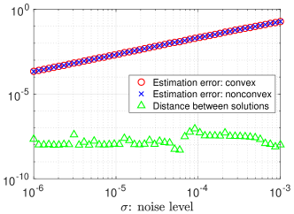
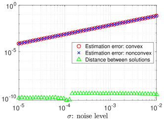
Figure 1: Left: blind deconvolution under Fourier design. Right: blind deconvolution under Gaussian design. Relative estimation errors of both $\bm{Z}_{\mathsf{cvx}}$ and $\bm{Z}_{\mathsf{ncvx}}$ and the relative distance between them vs. the noise level $\sigma$. The results are averaged over 20 independent trials.

In the second series of experiments, we report the numerical convergence of gradient descent (cf. Algorithm 1). We choose $K\in\{30,100,300,1000\}$ and let $m=10K$, with the noise level fixed at $\sigma=10^{-4}$. Figure 2 plots the relative Euclidean estimation error $\left\|\bm{h}^{t}\bm{x}^{t\mathsf{H}}-\bm{h}^{\star}\bm{x}^{\star\mathsf{H}}\right\|_{\text{F}}/\left\|\bm{h}^{\star}\bm{x}^{\star\mathsf{H}}\right\|_{\text{F}}$ vs. the iteration count. As can be seen from the plots, the nonconvex gradient algorithm studied here converges linearly (in fact, within around 200-300 iterations) before it hits an error floor. In addition, the relative error of blind deconvolution under Fourier design increases as the dimension $K$ increases, which is consistent with Theorem 2. While the relative error of blind deconvolution under Gaussian design remains generally the same across different choices of $K$, this can be explained by Theorem 4 since the ratio between $m$ and $K$ is kept to be $10$.

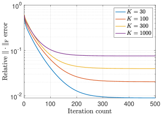
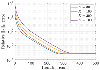
Figure 2: Left: blind deconvolution. Right: Gaussian design. Relative Euclidean error $\big{\|}\bm{h}^{t}\bm{x}^{t\mathsf{H}}-\bm{h}^{\star}\bm{x}^{\star\mathsf{H}}\big{\|}_{\mathrm{F}}$ vs. iteration count.

In the last series of experiments, we examine the necessity of the incoherence condition (2.1) empirically. The experiments are conducted with $\mu^{2}$ taking on 10 equidistant values from 3 to 30. For each choice of $\mu$, $\bm{h}^{\star}$ is generated by first setting the first $\mu^{2}$ entries to be 1 and the others 0 , and then normalizing it to have unit norm; $\bm{x}^{\star}$ is generated randomly from Gaussian distribution $\mathcal{N}(\bm{0},\bm{I}_{K})$ and then normalized to have unit norm. This way we guarantee that $\max_{1\leq j\leq m}|\bm{b}_{j}^{\mathsf{H}}\bm{h}^{\star}|=\mu/\sqrt{m}$. We fix $K=100$ and the noise level $\sigma=10^{-4}$ throughout. For each $\mu^{2}$ and $m$, 20 random trials are conducted. In each trial, we run convex and nonconvex algorithms until convergence or the maximum number of iterations is reached, and then report the relative Euclidean error $\|\bm{h}^{t}\bm{x}^{t\mathsf{H}}-\bm{h}^{\star}\bm{x}^{\star\mathsf{H}}\big{\|}_{\mathrm{F}}$. If the relative error is less than $0.1$, the trial is declared as successful. The proportion of successful recovery for convex and nonconvex problems are plotted in Figure 3, which suggests that sample complexity $m$ does scale linearly with $\mu^{2}$ for both problems and hence corroborates the theoretical results provided in Theorems 1 and 2.

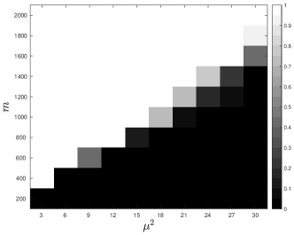
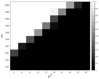
Figure 3: Left: nonconvex problem. Right: convex problem. Sample size $m$ vs. squared incoherence $\mu^{2}$. The scaled colormap represents the proportion of successful recovery out of 20 random trials.

5 Discussion

This paper has investigated the effectiveness of both convex relaxation and nonconvex optimization in solving bilinear systems of equations in the presence of random noise. We have demonstrated that a simple two-stage nonconvex algorithm solves the problem to optimal statistical accuracy within nearly linear time. Further, by establishing an intimate connection between convex programming and nonconvex optimization, we have established — for the first time — optimal statistical guarantees of convex relaxation when applied to blind deconvolution. Our results are established for two different types of design mechanisms: the random Fourier design and the Gaussian design. Our results considerably improve upon the state-of-the-art theory for blind deconvolution, and contribute towards demystifying the efficacy of optimization-based methods in solving this fundamental nonconvex problem.

Moving forward, the findings of this paper suggest multiple directions that merit further investigations. For instance, while the current paper adopts a balancing operation in each iteration of the nonconvex algorithm (cf. Algorithm 1), it might not be necessary in practice; in fact, numerical experiments suggest that the size of the scaling parameter $|\alpha^{t}|$ stays close to $1$ even without proper balancing. It would be interesting to investigate whether vanilla GD without rescaling is able to achieve comparable performance. In addition, the estimation guarantees provided in this paper might serve as a starting point for conducting uncertainty quantification for noisy blind deconvolution — namely, how to use it to construct valid and short confidence intervals for the unknowns. Going beyond blind deconvolution, it would be of interest to extend the current analysis to handle blind demixing — a problem that can be viewed as an extension of blind deconvolution beyond the rank-one setting (Ling and Strohmer, 2017, 2019; Dong and Shi, 2018). As can be expected, existing statistical guarantees for convex programming remain highly suboptimal for noisy blind demixing, and the analysis developed in the current paper suggests a feasible path towards closing the gap.

Appendix structure

Appendix A and B analyze the Fourier designs. In Appendix A, we present the analysis of the nonconvex gradient method and the proof of Theorem 2. Appendix B gives the complete proof of Theorem 1. In addition, Appendix C and D and provide proofs for the Gaussian designs, while Appendix C proves Theorem 4 and Appendix D proves Theorem 3. Appendix E justifies two minimax lower bounds in Theorem 5. Appendix F lists several useful lemmas and their proofs.

Appendix A Analysis: Nonconvex gradient method under Fourier design

Since the proof of Theorem 1 is built upon Theorem 2, we shall first present the proof of the nonconvex part. Without loss of generality, we assume that

$$\left\|\bm{h}^{\star}\right\|_{2}=\left\|\bm{x}^{\star}\right\|_{2}=1$$ (A.1)

throughout the proof. For the sake of notational convenience, for each iterate $(\bm{h}^{t},\bm{x}^{t})$ we define the following alignment parameters

$$\alpha^{t} \coloneqq\arg\min_{\alpha\in\mathbb{C}}\left\{\left\|\tfrac{1}{\overline{\alpha}}\bm{h}^{t}-\bm{h}^{\star}\right\|_{2}^{2}+\left\|\alpha\bm{x}^{t}-\bm{x}^{\star}\right\|_{2}^{2}\right\},$$ (A.2a)

$$\alpha^{t+1/2} \coloneqq\arg\min_{\alpha\in\mathbb{C}}\left\{\left\|\tfrac{1}{\overline{\alpha}}\bm{h}^{t+1/2}-\bm{h}^{\star}\right\|_{2}^{2}+\big{\|}\alpha\bm{x}^{t+1/2}-\bm{x}^{\star}\big{\|}_{2}^{2}\right\},$$ (A.2b)

which lead to the following simple relations

$$\alpha^{t+1}=\sqrt{\frac{\left\|\bm{x}^{t+1/2}\right\|_{2}}{\left\|\bm{h}^{t+1/2}\right\|_{2}}}\alpha^{t+1/2}\qquad\text{and}\qquad\mathsf{dist}\big{(}\bm{z}^{t+1/2},\bm{z}^{\star}\big{)}=\mathsf{dist}\big{(}\bm{z}^{t+1},\bm{z}^{\star}\big{)}.$$ (A.3)

With these in place, attention should be directed to the properly rescaled iterate

$$\widetilde{\bm{z}}^{t+1/2}=\big{(}\widetilde{\bm{h}}^{t+1/2},\widetilde{\bm{x}}^{t+1/2}\big{)} :=\big{(}\tfrac{1}{\overline{\alpha^{t+1/2}}}\bm{h}^{t+1/2},\alpha^{t+1/2}\bm{x}^{t+1/2}\big{)},$$ (A.4a)

$$\widetilde{\bm{z}}^{t}=\big{(}\widetilde{\bm{h}}^{t},\widetilde{\bm{x}}^{t}\big{)} :=\big{(}\tfrac{1}{\overline{\alpha^{t}}}\bm{h}^{t},\alpha^{t}\bm{x}^{t}\big{)}.$$ (A.4b)

Additionally, we shall also define

$$\widehat{\bm{z}}^{t+1/2}=(\widehat{\bm{h}}^{t+1/2},\widehat{\bm{x}}^{t+1/2}) :=\big{(}\tfrac{1}{\overline{\alpha^{t}}}\bm{h}^{t+1/2},\alpha^{t}\bm{x}^{t+1/2}\big{)}$$ (A.5a)

$$\widehat{\bm{z}}^{t+1}=(\widehat{\bm{h}}^{t+1},\widehat{\bm{x}}^{t+1}) :=\big{(}\tfrac{1}{\overline{\alpha^{t}}}\bm{h}^{t+1},\alpha^{t}\bm{x}^{t+1}\big{)}$$ (A.5b)

that are rescaled in a different way, which will appear often in the analysis.

A.1 Induction hypotheses

Our analysis is inductive in nature; more concretely, we aim to justify the following set of hypotheses by induction:

$$\mathsf{dist}\left(\bm{z}^{t},\bm{z}^{\star}\right) \leq\big{\|}\widehat{\bm{z}}^{t-1/2}-\bm{z}^{\star}\big{\|}_{2}\leq\rho\mathsf{dist}\left(\bm{z}^{t-1},\bm{z}^{\star}\right)+C_{1}\eta\left(\lambda+\sigma\sqrt{K\log m}\right),$$ (A.6a)

$$\max_{1\leq l\leq m}\left|\bm{a}_{l}^{\mathsf{H}}\left(\widetilde{\bm{x}}^{t}-\bm{x}^{\star}\right)\right| \leq C_{3}\left(\sqrt{\frac{\mu^{2}K\log^{2}m}{m}}+\sqrt{\log m}\left(\lambda+\sigma\sqrt{K\log m}\right)\right),$$ (A.6b)

$$\max_{1\leq l\leq m}\big{|}\bm{b}_{l}^{\mathsf{H}}\widetilde{\bm{h}}^{t}\big{|} \leq C_{4}\left(\frac{\mu\log^{2}m}{\sqrt{m}}+\sigma\right),$$ (A.6c)

where $$\rho=1-\eta/16 C_{1},C_{3},C_{4}>0 0<t\leq t_{0} 0\leq t\leq t_{0}$$ and are some universal constants. Here, the hypothesis (A.6a) is made for all , while the hypotheses (A.6b) and (A.6c) are made for all . Clearly, if the hypotheses (A.6a) can be established, then simple recursion yields

$$\mathsf{dist}\left(\bm{z}^{t},\bm{z}^{\star}\right) \lesssim\rho^{t}\mathsf{dist}\left(\bm{z}^{0},\bm{z}^{\star}\right)+\frac{C_{1}\eta\left(\lambda+\sigma\sqrt{K\log m}\right)}{1-\rho}$$

$$=\rho^{t}\mathsf{dist}\left(\bm{z}^{0},\bm{z}^{\star}\right)+\frac{C_{1}\left(\lambda+\sigma\sqrt{K\log m}\right)}{c_{\rho}},\qquad 0\leq t\leq t_{0}$$ (A.6d)

as claimed. Moreover, one might naturally wonder why we are in need of the additional hypotheses (A.6b) and (A.6c) that might seem irrelevant at first glance. As it turns out, these two hypotheses — which characterize certain incoherence conditions of the iterates w.r.t. the design vectors — play a pivotal role in the analysis, as they enable some sort of “restricted strong convexity” that proves crucial for guaranteeing linear convergence.

In addition, the analysis also relies upon the following important properties of the initialization, which we shall establish momentarily:

$$\mathsf{dist}\left(\bm{z}^{0},\bm{z}^{\star}\right) \lesssim\sqrt{\frac{\mu^{2}K\log m}{m}}+\sigma\sqrt{K\log m},$$ (A.6e)

$$\max_{1\leq j\leq m}\left|\bm{a}_{j}^{\mathsf{H}}\big{(}\widetilde{\bm{x}}^{0}-\bm{x}^{\star}\big{)}\right| \lesssim\sqrt{\frac{\mu^{2}K\log^{2}m}{m}}+\sigma\sqrt{K}\log m,$$ (A.6f)

$$\max_{1\leq l\leq m}\big{|}\bm{b}_{l}^{\mathsf{H}}\widetilde{\bm{h}}^{0}\big{|} \lesssim\frac{\mu\log^{2}m}{\sqrt{m}}+\sigma,$$ (A.6g)

$$\big{|}|\alpha^{0}|-1\big{|} \leq 1/4.$$ (A.6h)

A.2 Preliminaries

Before proceeding to the proof, we gather several preliminary facts that will be useful throughout.

A.2.1 Wirtinger calculus and notation

Given that this problem concerns complex-valued vectors/matrices, we find it convenient to work with Wirtinger calculus; see Candes et al. [2015, Section 6] and Ma et al. [2018, Section D.3.1] for a brief introduction. Here, we shall simply record below the expressions for the Wirtinger gradient and the Wirtinger Hessian w.r.t. the objective function $f(\cdot)$ defined in (1.4):

$$\nabla_{\bm{h}}f\left(\bm{h},\bm{x}\right)= \sum_{j=1}^{m}\left(\bm{b}_{j}^{\mathsf{H}}\bm{hx}^{\mathsf{H}}\bm{a}_{j}-y_{j}\right)\bm{b}_{j}\bm{a}_{j}^{\mathsf{H}}\bm{x}+\lambda\bm{h},$$ (A.7a)

$$\nabla_{\bm{x}}f\left(\bm{h},\bm{x}\right)= \sum_{j=1}^{m}\overline{\left(\bm{b}_{j}^{\mathsf{H}}\bm{hx}^{\mathsf{H}}\bm{a}_{j}-y_{j}\right)}\bm{a}_{j}\bm{b}_{j}^{\mathsf{H}}\bm{h}+\lambda\bm{x},$$ (A.7b)

$$\nabla^{2}f\left(\bm{h},\bm{x}\right)= \left[\begin{array}[]{cc}\bm{A}&\bm{B}\\ \bm{B}^{\mathsf{H}}&\overline{\bm{A}}\end{array}\right],$$ (A.7e)

where

$$\bm{A}:= \left[\begin{array}[]{cc}\sum_{j=1}^{m}\left|\bm{a}_{j}^{\mathsf{H}}\bm{x}\right|{}^{2}\bm{b}_{j}\bm{b}_{j}^{\mathsf{H}}+\lambda&\sum_{j=1}^{m}\left(\bm{b}_{j}^{\mathsf{H}}\bm{hx}^{\mathsf{H}}\bm{a}_{j}-y_{j}\right)\bm{b}_{j}\bm{a}_{j}^{\mathsf{H}}\\ \sum_{j=1}^{m}\left[\left(\bm{b}_{j}^{\mathsf{H}}\bm{hx}^{\mathsf{H}}\bm{a}_{j}-y_{j}\right)\bm{b}_{j}\bm{a}_{j}^{\mathsf{H}}\right]^{\mathsf{H}}&\sum_{j=1}^{m}\left|\bm{b}_{j}^{\mathsf{H}}\bm{h}\right|{}^{2}\bm{a}_{j}\bm{a}_{j}^{\mathsf{H}}+\lambda\end{array}\right]\in\mathbb{C}^{2K\times 2K},$$

$$\bm{B}:= \left[\begin{array}[]{cc}\bm{0}&\sum_{j=1}^{m}\bm{b}_{j}\bm{b}_{j}^{\mathsf{H}}\bm{h}\left(\bm{a}_{j}\bm{a}_{j}^{\mathsf{H}}\bm{x}\right)^{\mathsf{H}}\\ \sum_{j=1}^{m}\bm{a}_{j}\bm{a}_{j}^{\mathsf{H}}\bm{x}\left(\bm{b}_{j}\bm{b}_{j}^{\mathsf{H}}\bm{h}\right)^{\mathsf{H}}&\bm{0}\end{array}\right]\in\mathbb{C}^{2K\times 2K}.$$

Throughout this paper, we shall often use $f\left(\bm{h},\bm{x}\right)$ and $f\left(\bm{z}\right)$ interchangeably for any $\bm{z}=\footnotesize\left[\begin{array}[]{c}\bm{h}\\ \bm{x}\end{array}\right]$, whenever it is clear from the context.

Before proceeding, we present two useful properties of the operator $\mathcal{A}$ and the design vectors $\{\bm{b}_{j}\}_{j=1}^{m}$.

Lemma 1.

For $\mathcal{A}$ defined in (B.3), with probability at least $1-m^{-\gamma}$,

$$\left\|\mathcal{A}\right\|\leq\sqrt{2K\log K+\gamma\log m}.$$

Proof.

See Li et al. [2019, Lemma 5.12].∎

Lemma 2.

For any $m\geq 3$ and any $1\leq l\leq m$, we have

$$\sum_{j=1}^{m}\left|\bm{b}_{l}^{\mathsf{H}}\bm{b}_{j}\right|\leq 4\log m.$$

Proof.

See Ma et al. [2018, Lemma 48].∎

A.2.2 Leave-one-out auxiliary sequences

The key to establishing the incoherence hypotheses (A.6b) and (A.6c) is to introduce a collection of auxiliary leave-one-out sequences — an approach first introduced by Ma et al. [2018]. Specifically, for each $1\leq l\leq m$, define the leave-one-out loss function as follows

$$f^{(l)}\left(\bm{h},\bm{x}\right)\coloneqq\sum_{j:j\neq l}\left|\bm{b}_{j}^{\mathsf{H}}\bm{h}\bm{x}^{\mathsf{H}}\bm{a}_{j}-y_{j}\right|^{2}+\lambda\left\|\bm{h}\right\|_{2}^{2}+\lambda\left\|\bm{x}\right\|_{2}^{2},$$

which is obtained by discarding the $l$th sample. We then generate the auxiliary sequence $\{\bm{h}^{(t),l},\bm{x}^{(t),l}\}_{t\geq 0}$ by running the same nonconvex algorithm w.r.t. $f^{(l)}(\cdot,\cdot)$, as summarized in Algorithm 2. In a nutshell, the resulting leave-one-out sequence $\{\bm{h}^{(t),l},\bm{x}^{(t),l}\}_{t\geq 0}$ is statistically independent from the design vector $\bm{a}_{l}$ and is expected to stay exceedingly close to the original sequence (given that only a single sample is dropped), which in turn facilitate the analysis of the correlation of $\bm{a}_{l}$ and $\bm{x}^{t}$ as claimed in (A.6b). In the mean time, this strategy also proves useful in controlling the correlation of $\bm{b}_{l}$ and $\bm{h}^{t}$ as in (A.6c), albeit with more delicate arguments.

Algorithm 2 The $l$th leave-one-out sequence for nonconvex blind deconvolution

  Input: $\left\{\bm{a}_{j}\right\}_{1\leq j\leq m,j\neq l}$, $\left\{\bm{b}_{j}\right\}_{1\leq j\leq m,j\neq l}$ and $\left\{y_{j}\right\}_{1\leq j\leq m,j\neq l}$.

  Spectral initialization: let $\sigma_{1}\left(\bm{M}^{\left(l\right)}\right)$, $\check{\bm{h}}^{0,\left(l\right)}$ and $\check{\bm{x}}^{0,\left(l\right)}$ be the leading singular value, the leading left and right singular vectors of

$$\bm{M}^{\left(l\right)}\coloneqq\sum_{j:j\neq l}y_{j}\bm{b}_{j}\bm{a}_{j}^{\mathsf{H}},$$ (A.8)

respectively. Set $\bm{h}^{0,\left(l\right)}=\sqrt{\sigma_{1}\left(\bm{M}^{\left(l\right)}\right)}\,\check{\bm{h}}^{0,\left(l\right)}$ and $\bm{x}^{0,\left(l\right)}=\sqrt{\sigma_{1}\left(\bm{M}^{\left(l\right)}\right)}\,\check{\bm{x}}^{0,\left(l\right)}$.

  Gradient updates: for $t=0,1,\ldots,t_{0}-1$ do

  

$$\begin{aligned} \left[\begin{array}[]{c}\bm{h}^{t+1/2,\left(l\right)}\\ \bm{x}^{t+1/2,\left(l\right)}\end{array}\right]=&\left[\begin{array}[]{c}\bm{h}^{t,\left(l\right)}\\ \bm{x}^{t,\left(l\right)}\end{array}\right]-\eta\left[\begin{array}[]{c}\nabla_{\bm{h}}f^{\left(l\right)}\left(\bm{h}^{t},\bm{x}^{t}\right)\\ \nabla_{\bm{x}}f^{\left(l\right)}\left(\bm{h}^{t},\bm{x}^{t}\right)\end{array}\right],\\ \left[\begin{array}[]{c}\bm{h}^{t+1,\left(l\right)}\\ \bm{x}^{t+1,\left(l\right)}\end{array}\right]=&\left[\begin{array}[]{c}\sqrt{\frac{\left\|\bm{x}^{t+1/2,\left(l\right)}\right\|_{2}}{\left\|\bm{h}^{t+1/2,\left(l\right)}\right\|_{2}}}\bm{h}^{t+1/2,\left(l\right)}\\ \sqrt{\frac{\left\|\bm{h}^{t+1/2,\left(l\right)}\right\|_{2}}{\left\|\bm{x}^{t+1/2,\left(l\right)}\right\|_{2}}}\bm{x}^{t+1/2,\left(l\right)}\end{array}\right].\end{aligned}$$ (A.9a)

Similar to the notation adopted for the original sequence, we shall define the alignment parameter for the leave-one-out sequence as follows

$$\alpha^{t,(l)} \coloneqq\arg\min_{\alpha\in\mathbb{C}}\left\{\left\|\tfrac{1}{\overline{\alpha}}\bm{h}^{t,(l)}-\bm{h}^{\star}\right\|_{2}^{2}+\big{\|}\alpha\bm{x}^{t,(l)}-\bm{x}^{\star}\big{\|}_{2}^{2}\right\},$$ (A.10a)

$$\alpha^{t+1/2,(l)} \coloneqq\arg\min_{\alpha\in\mathbb{C}}\left\{\left\|\tfrac{1}{\overline{\alpha}}\bm{h}^{t+1/2,(l)}-\bm{h}^{\star}\right\|_{2}^{2}+\big{\|}\alpha\bm{x}^{t+1/2,(l)}-\bm{x}^{\star}\big{\|}_{2}^{2}\right\},$$ (A.10b)

along with the properly rescaled iterates

$$\widetilde{\bm{z}}^{t,\left(l\right)}=\left[\begin{array}[]{c}\widetilde{\bm{h}}^{t,(l)}\\ \widetilde{\bm{x}}^{t,(l)}\end{array}\right] :=\left[\begin{array}[]{c}\frac{1}{\overline{\alpha^{t,\left(l\right)}}}\bm{h}^{t,(l)}\\ \alpha^{t,(l)}\bm{x}^{t,(l)}\end{array}\right],$$ (A.11e)

$$\widetilde{\bm{z}}^{t+1/2,\left(l\right)}=\left[\begin{array}[]{c}\widetilde{\bm{h}}^{t+1/2,(l)}\\ \widetilde{\bm{x}}^{t+1/2,(l)}\end{array}\right] :=\left[\begin{array}[]{c}\frac{1}{\overline{\alpha^{t+1/2,\left(l\right)}}}\bm{h}^{t+1/2,(l)}\\ \alpha^{t+1/2,(l)}\bm{x}^{t+1/2,(l)}\end{array}\right].$$ (A.11j)

Further we define the alignment parameter between $\bm{z}^{t,\left(l\right)}$ and $\widetilde{\bm{z}}^{t}$ as

$$\alpha_{\text{\text{mutual}}}^{t,\left(l\right)} \coloneqq\arg\min_{\alpha\in\mathbb{C}}\left\{\left\|\tfrac{1}{\overline{\alpha}}\bm{h}^{t,\left(l\right)}-\tfrac{1}{\overline{\alpha^{t}}}\bm{h}^{t}\right\|_{2}^{2}+\left\|\alpha\bm{x}^{t,\left(l\right)}-\alpha^{t}\bm{x}^{t}\right\|_{2}^{2}\right\},$$ (A.12a)

$$\alpha_{\text{\text{mutual}}}^{t+1/2,\left(l\right)} \coloneqq\arg\min_{\alpha\in\mathbb{C}}\left\{\left\|\tfrac{1}{\overline{\alpha}}\bm{h}^{t+1/2,\left(l\right)}-\tfrac{1}{\overline{\alpha^{t+1/2}}}\bm{h}^{t+1/2}\right\|_{2}^{2}+\left\|\alpha\bm{x}^{t+1/2,\left(l\right)}-\alpha^{t+1/2}\bm{x}^{t+1/2}\right\|_{2}^{2}\right\}.$$ (A.12b)

Hereafter, we shall also denote

$$\widehat{\bm{z}}^{t,\left(l\right)}:=\left[\begin{array}[]{c}\widehat{\bm{h}}^{t,\left(l\right)}\\ \widehat{\bm{x}}^{t,\left(l\right)}\end{array}\right] =\left[\begin{array}[]{c}\tfrac{1}{\overline{\alpha_{\text{mutual}}^{t,\left(l\right)}}}\bm{h}^{t,\left(l\right)}\\ \alpha_{\text{mutual}}^{t,\left(l\right)}\bm{x}^{t,\left(l\right)}\end{array}\right],$$ (A.13e)

$$\widehat{\bm{z}}^{t+1/2,\left(l\right)}:=\left[\begin{array}[]{c}\widehat{\bm{h}}^{t+1/2,\left(l\right)}\\ \widehat{\bm{x}}^{t+1/2,\left(l\right)}\end{array}\right] =\left[\begin{array}[]{c}\tfrac{1}{\overline{\alpha_{\text{mutual}}^{t+1/2,\left(l\right)}}}\bm{h}^{t+1/2,\left(l\right)}\\ \alpha_{\text{mutual}}^{t+1/2,\left(l\right)}\bm{x}^{t+1/2,\left(l\right)}\end{array}\right].$$ (A.13j)

A.2.3 Additional induction hypotheses

In addition to the set of induction hypotheses already listed in (A.6), we find it convenient to include the following hypotheses concerning the leave-one-out sequences. Specifically, for any $0<t\leq t_{0}$ and any $1\leq l\leq m$, the hypotheses claim that

$$\mathsf{dist}\big{(}\bm{z}^{t,\left(l\right)},\widetilde{\bm{z}}^{t}\big{)} \leq C_{2}\left(\frac{\mu}{\sqrt{m}}\sqrt{\frac{\mu^{2}K\log^{9}m}{m}}+\frac{\sigma}{\log^{2}m}\right)$$ (A.14a)

$$\big{\|}\widetilde{\bm{z}}^{t,\left(l\right)}-\widetilde{\bm{z}}^{t}\big{\|}_{2} \lesssim C_{2}\left(\frac{\mu}{\sqrt{m}}\sqrt{\frac{\mu^{2}K\log^{9}m}{m}}+\frac{\sigma}{\log^{2}m}\right)$$ (A.14b)

$$\mathsf{dist}\big{(}\bm{z}^{0,(l)},\bm{z}^{\star}\big{)} \lesssim\sqrt{\frac{\mu^{2}K\log m}{m}}+\sigma\sqrt{K\log m}$$ (A.14c)

$$\mathsf{dist}\big{(}\bm{z}^{0,\left(l\right)},\widetilde{\bm{z}}^{0}\big{)} \lesssim\frac{\mu}{\sqrt{m}}\sqrt{\frac{\mu^{2}K\log^{5}m}{m}}+\frac{\sigma}{\log^{2}m}$$ (A.14d)

for some constant $C_{2}\gg C_{4}^{2}$. Furthermore, there are several immediate consequences of the hypotheses (A.6) and (A.14) that are also useful in the analysis, which we gather as follows. Note that the notation $(\widetilde{\bm{h}}^{t},\widetilde{\bm{x}}^{t})$, $(\widehat{\bm{h}}^{t},\widehat{\bm{x}}^{t})$, $(\widehat{\bm{h}}^{t,(l)},\widehat{\bm{x}}^{t,(l)})$ and $\alpha^{t}$ has been defined in (A.4b), (A.5b), (A.13e) and (A.2a), respectively.

Lemma 3.

Instate the notation and assumptions in Theorem 2. For $t\geq 0$, suppose that the hypotheses (A.6) and (A.14) hold in the first $t$ iterations. Then there exist some constants $C_{1},C>0$ such that for any $1\leq l\leq m$,

$$\mathsf{dist}\left(\bm{z}^{t},\bm{z}^{\star}\right) \leq C_{1}\left(\sqrt{\frac{\mu^{2}K\log m}{m}}+\lambda+\sigma\sqrt{K\log m}\right),$$ (A.15a)

$$\left\|\bm{h}^{t}\big{(}\bm{x}^{t}\big{)}^{\mathsf{H}}-\bm{h}^{\star}\bm{x}^{\mathsf{\star H}}\right\| \leq C\left(\sqrt{\frac{\mu^{2}K\log m}{m}}+\lambda+\sigma\sqrt{K\log m}\right),$$ (A.15b)

$$\big{\|}\widetilde{\bm{z}}^{t,\left(l\right)}-\bm{z}^{\star}\big{\|}_{2} \leq 2C_{1}\left(\sqrt{\frac{\mu^{2}K\log m}{m}}+\lambda+\sigma\sqrt{K\log m}\right),$$ (A.15c)

$$\frac{1}{2}\leq\left\|\widetilde{\bm{x}}^{t}\right\|_{2}\leq\frac{3}{2}, \qquad\frac{1}{2}\leq\big{\|}\widetilde{\bm{h}}^{t}\big{\|}_{2}\leq\frac{3}{2},$$ (A.15d)

$$\frac{1}{2}\leq\big{\|}\widetilde{\bm{x}}^{t,\left(l\right)}\big{\|}_{2}\leq\frac{3}{2}, \qquad\frac{1}{2}\leq\big{\|}\widetilde{\bm{h}}^{t,\left(l\right)}\big{\|}_{2}\leq\frac{3}{2},$$ (A.15e)

$$\frac{1}{2}\leq\big{\|}\widehat{\bm{x}}^{t,\left(l\right)}\big{\|}_{2}\leq\frac{3}{2}, \qquad\frac{1}{2}\leq\big{\|}\widehat{\bm{h}}^{t,\left(l\right)}\big{\|}_{2}\leq\frac{3}{2}.$$ (A.15f)

In addition, if $$t>0$$, then one also has

$$\big{\|}\widehat{\bm{z}}^{t-1/2}-\bm{z}^{\star}\big{\|}_{2} \leq C\left(\sqrt{\frac{\mu^{2}K\log m}{m}}+\lambda+\sigma\sqrt{K\log m}\right).$$ (A.15g)

Proof.

See Appendix A.4.∎

A.3 Inductive analysis

In this subsection, we carry out the analysis by induction.

A.3.1 Step 1: Characterizing local geometry

Similar to Ma et al. [2018, Lemma 14], local linear convergence is made possible when some sort of restricted strong convexity and smoothness are present simultaneously. To be specific, define the following squared loss that excludes the regularization term

$$f_{\mathsf{reg}\text{-}\mathsf{free}}\left(\bm{z}\right)=f_{\mathsf{reg}\text{-}\mathsf{free}}\left(\bm{h},\bm{x}\right):=\sum_{j=1}^{m}\big{|}\bm{b}_{j}^{\mathsf{H}}\bm{hx}^{\mathsf{H}}\bm{a}_{j}-y_{j}\big{|}^{2}.$$ (A.16)

Our result is this:

Lemma 4.

Let $\delta:=c/\log^{2}m$ for some sufficiently small constant $c>0$. Suppose that $m\geq C\mu^{2}K\log^{9}m$ for some sufficiently large constant $C>0$ and that $\sigma\sqrt{K\log^{5}m}\leq c_{1}$ for some sufficiently small constant $c_{1}>0$. Then with probability $1-O\left(m^{-10}+e^{-K}\log m\right)$, one has

$$\bm{u}^{\mathsf{H}}\left[\bm{D}\nabla^{2}f\left(\bm{z}\right)+\nabla^{2}f\left(\bm{z}\right)\bm{D}\right]\bm{u} \geq\left\|\bm{u}\right\|_{2}^{2}/8\quad\text{and}$$

$$\left\|\nabla^{2}f\left(\bm{z}\right)\right\| \leq 4$$

simultaneously for all points

$$\bm{z}=\left[\begin{array}[]{c}\bm{h}\\ \bm{x}\end{array}\right],\quad\bm{u}=\left[\begin{array}[]{c}\bm{h}_{1}-\bm{h}_{2}\\ \bm{x}_{1}-\bm{x}_{2}\\ \overline{\bm{h}_{1}-\bm{h}_{2}}\\ \overline{\bm{x}_{1}-\bm{x}_{2}}\end{array}\right]\quad\text{and}\quad\bm{D}=\left[\begin{array}[]{cccc}\gamma_{1}\bm{I}_{K}\\ &\gamma_{2}\bm{I}_{K}\\ &&\gamma_{1}\bm{I}_{K}\\ &&&\gamma_{2}\bm{I}_{K}\end{array}\right]$$

obeying the following properties:

• $\bm{z}$ satisfies

  $$\max\left\{\left\|\bm{h}-\bm{h}^{\star}\right\|_{2},\left\|\bm{x}-\bm{x}^{\star}\right\|_{2}\right\} \leq\delta,$$

  $$\max_{1\leq j\leq m}\left|\bm{a}_{j}^{\mathsf{H}}\left(\bm{x}-\bm{x}^{\star}\right)\right| \leq 2C_{3}\tfrac{1}{\log^{3/2}m},$$

  $$\max_{1\leq j\leq m}\left|\bm{b}_{j}^{\mathsf{H}}\bm{h}\right| \leq 2C_{4}\Big{(}\tfrac{\mu\log^{2}m}{\sqrt{m}}+\sigma\Big{)};$$

• $\bm{z}_{1}:=\left(\bm{h}_{1},\bm{x}_{1}\right)$ is aligned with $\bm{z}_{2}:=\left(\bm{h}_{2},\bm{x}_{2}\right)$ in the sense that $\|\bm{z}_{1}-\bm{z}_{2}\|_{2}=\mathsf{dist}(\bm{z}_{1},\bm{z}_{2})$; in addition, they satisfy

  $$\max\left\{\left\|\bm{h}_{1}-\bm{h}^{\star}\right\|_{2},\left\|\bm{h}_{2}-\bm{h}^{\star}\right\|_{2},\left\|\bm{x}_{1}-\bm{x}^{\star}\right\|_{2},\left\|\bm{x}_{2}-\bm{x}^{\star}\right\|_{2}\right\}\leq\delta;$$

• $\gamma_{1},\gamma_{2}\in\mathbb{R}$ and obey

  $$\max\left\{\left|\gamma_{1}-1\right|,\left|\gamma_{2}-1\right|\right\}\leq\delta.$$

Proof.

See Appendix A.6.∎

In words, the function $f(\cdot)$ resembles a strongly convex and smooth function when we restrict attention to (i) a highly restricted set of points $\bm{z}$ and (ii) a highly special set of directions $\bm{u}$.

A.3.2 Step 2: $\ell_{2}$ error contraction

Next, we demonstrate that under the hypotheses (A.6) for the $t$th iteration, the next iterate will undergo $\ell_{2}$ error contraction, as long as the stepsize is properly chosen. The proof is largely based on the restricted strong convexity and smoothness established in Lemma 4.

Lemma 5.

Set $\lambda=C_{\lambda}\sigma\sqrt{K\log m}$ for some large constant $C_{\lambda}>0$. The stepsize parameter $\eta>0$ in Algorithm 2 is taken to be some sufficiently small constant. There exists some constant $C>0$ such that with probability at least $1-O\left(m^{-100}+e^{-CK}\log m\right)$, if the hypotheses (A.6) hold true at the $t$th iteration, then

$$\mathsf{dist}\left(\bm{z}^{t+1},\bm{z}^{\star}\right) \leq\big{\|}\widehat{\bm{z}}^{t+1/2}-\bm{z}^{\star}\big{\|}_{2}\leq\rho\mathsf{dist}\left(\bm{z}^{t},\bm{z}^{\star}\right)+C_{1}\eta\left(\lambda+\sigma\sqrt{K\log m}\right)$$ (A.17)

for some constants $\rho=1-\eta/16$ and $C_{1}>0$.

Proof.

See Appendix A.7.∎

To establish this lemma and many other results, we need to ensure that the alignment parameters and the sizes of the iterates do not change much, as stated below.

Corollary 1.

Instate the notation and assumptions in Theorem 2. For an integer $t>0$, suppose that the hypotheses (A.6) and (A.14) hold in the first $t-1$ iterations. Then there exists some constant $C>0$ such that for any $1\leq l\leq m$, one has

$$\left|\left|\alpha^{t}\right|-1\right| \lesssim\mathsf{dist}\left(\widetilde{\bm{z}}^{t},\bm{z}^{\star}\right)\lesssim\sqrt{\frac{\mu^{2}K\log m}{m}}+\lambda+\sigma\sqrt{K\log m},$$ (A.18a)

$$\left|\frac{\alpha^{t-1/2}}{\alpha^{t-1}}-1\right| \lesssim\eta\left(\sqrt{\frac{\mu^{2}K\log m}{m}}+\lambda+\sigma\sqrt{K\log m}\right),$$ (A.18b)

$$\left|\left|\alpha_{\mathrm{mutual}}^{t,\left(l\right)}\right|-1\right| \lesssim\big{\|}\widehat{\bm{z}}^{t,\left(l\right)}-\bm{z}^{\star}\big{\|}_{2}\lesssim\sqrt{\frac{\mu^{2}K\log m}{m}}+\lambda+\sigma\sqrt{K\log m},$$ (A.18c)

$$\frac{1}{2}\leq\left\|\bm{x}^{t}\right\|_{2}\leq\frac{3}{2}, \qquad\frac{1}{2}\leq\left\|\bm{h}^{t}\right\|_{2}\leq\frac{3}{2},$$ (A.18d)

$$\frac{1}{2}\leq\big{\|}\bm{x}^{t,\left(l\right)}\big{\|}_{2}\leq\frac{3}{2}, \qquad\frac{1}{2}\leq\big{\|}\bm{h}^{t,\left(l\right)}\big{\|}_{2}\leq\frac{3}{2}$$ (A.18e)

with probability at least $1-O\left(m^{-100}+e^{-CK}\log m\right)$.

Proof.

See Appendix A.5.∎

A.3.3 Step 3: Leave-one-out proximity

We then move on to justifying the close proximity of the leave-one-out sequences and the original sequences, as stated in the hypothesis (A.14a).

Lemma 6.

Suppose the sample complexity obeys $m\geq C\mu^{2}K\log^{9}m$ for some sufficiently large constant $C>0$. If the hypotheses (A.6a)-(A.6c) hold for the $t$th iteration, then with probability at least $1-O\left(m^{-100}+me^{-cK}\right)$ for some constant $c>0$, one has

$$\max_{1\leq l\leq m}\mathsf{dist}\big{(}\bm{z}^{t+1,\left(l\right)},\widetilde{\bm{z}}^{t+1}\big{)} \leq C_{2}\left(\frac{\mu}{\sqrt{m}}\sqrt{\frac{\mu^{2}K\log^{9}m}{m}}+\frac{\sigma}{\log^{2}m}\right)$$ (A.19a)

$$\text{and}\qquad\max_{1\leq l\leq m}\big{\|}\widetilde{\bm{z}}^{t+1,\left(l\right)}-\widetilde{\bm{z}}^{t+1}\big{\|}_{2} \lesssim C_{2}\left(\frac{\mu}{\sqrt{m}}\sqrt{\frac{\mu^{2}K\log^{9}m}{m}}+\frac{\sigma}{\log^{2}m}\right),$$ (A.19b)

provided that the stepsize $\eta>0$ is some sufficiently small constant.

Proof.

See Appendix A.8.∎

A.3.4 Step 4: Establishing incoherence

The next step is to establish the hypotheses concerning incoherence, namely, (A.6b) and (A.6c) for the $(t+1)$-th iteration.

We start with the incoherence of $\bm{a}_{l}$ and $\bm{x}^{t+1}$, which is much easier to handle. The standard Gaussian concentration inequality gives

$$\max_{1\leq l\leq m}\left|\bm{a}_{l}^{\mathsf{H}}\big{(}\widetilde{\bm{x}}^{t+1,\left(l\right)}-\bm{x}^{\star}\big{)}\right|\leq 20\sqrt{\log m}\max_{1\leq l\leq m}\big{\|}\widetilde{\bm{x}}^{t+1,\left(l\right)}-\bm{x}^{\star}\big{\|}_{2}$$ (A.20)

with probability exceeding $1-O\left(m^{-100}\right)$. Then the triangle inequality and Cauchy-Schwarz inequality yield

$$\left|\bm{a}_{l}^{\mathsf{H}}\big{(}\widetilde{\bm{x}}^{t+1}-\bm{x}^{\star}\big{)}\right| \leq\left|\bm{a}_{l}^{\mathsf{H}}\big{(}\widetilde{\bm{x}}^{t+1}-\widetilde{\bm{x}}^{t+1,\left(l\right)}\big{)}\right|+\left|\bm{a}_{l}^{\mathsf{H}}\big{(}\widetilde{\bm{x}}^{t+1,\left(l\right)}-\bm{x}^{\star}\big{)}\right|$$

$$\leq\left\|\bm{a}_{l}\right\|_{2}\big{\|}\widetilde{\bm{x}}^{t+1}-\widetilde{\bm{x}}^{t+1,\left(l\right)}\big{\|}_{2}+\left|\bm{a}_{l}^{\mathsf{H}}\big{(}\widetilde{\bm{x}}^{t+1,\left(l\right)}-\bm{x}^{\star}\big{)}\right|$$

$$\leq 10\sqrt{K}C_{2}\left(\frac{\mu}{\sqrt{m}}\sqrt{\frac{\mu^{2}K\log^{9}m}{m}}+\frac{\sigma}{\log^{2}m}\right)$$

$$\quad+20\sqrt{\log m}\cdot 2C_{1}\left(\sqrt{\frac{\mu^{2}K\log m}{m}}+\lambda+\sigma\sqrt{K\log m}\right)$$

$$\leq C_{3}\left(\sqrt{\frac{\mu^{2}K\log^{2}m}{m}}+\lambda+\sigma\sqrt{K}\log m\right),$$ (A.21)

where $C_{3}\gg C_{1}$, the penultimate inequality follows from (F.2), (A.19b), (A.20) and (A.15c). This establishes the hypothesis (A.6b) for the $(t+1)$-th iteration.

Regarding the incoherence of $\bm{b}_{l}$ and $\bm{h}^{t+1}$ (as stated in the hypothesis (A.6c)), we have the following lemma.

Lemma 7.

Suppose the sample complexity obeys $m\geq C\mu^{2}K\log^{9}m$ for some sufficiently large constant $C>0$ and $\lambda=C_{\lambda}\sigma\sqrt{K\log m}$ for some absolute constant $C_{\lambda}>0$. If the hypotheses (A.6a)-(A.6c) hold for the $t$th iteration, then with probability exceeding $1-O\left(m^{-100}+me^{-CK}\right)$ for some constant $C>0$, one has

$$\max_{1\leq l\leq m}\big{|}\bm{b}_{l}^{\mathsf{H}}\widetilde{\bm{h}}^{t+1}\big{|}\leq C_{4}\left(\frac{\mu}{\sqrt{m}}\log^{2}m+\sigma\right),$$

as long as $C_{4}>0$ is some sufficiently large constant and $\eta>0$ is taken to be some sufficiently small constant.

Proof.

See Appendix A.9.∎

A.3.5 The base case: Spectral initialization

To finish the induction analysis, it remains to justify the induction hypotheses for the base case. Recall that $\sigma\left(\bm{M}\right),\check{\bm{h}}^{0}$ and $\check{\bm{x}}^{0}$ denote respectively the leading singular value, the left and the right singular vectors of

$$\bm{M}\coloneqq\sum_{j=1}^{m}y_{j}\bm{b}_{j}\bm{a}_{j}^{\mathsf{H}}.$$

The spectral initialization procedure sets $\bm{h}^{0}=\sqrt{\sigma_{1}\left(\bm{M}\right)}\check{\bm{h}}^{0}$ and $\bm{x}^{0}=\sqrt{\sigma_{1}\left(\bm{M}\right)}\check{\bm{x}}^{0}$.

To begin with, the following lemma guarantees that $\left(\bm{h}^{0},\bm{x}^{0}\right)$ satisfies the desired conditions (A.6e) and (A.6h).

Lemma 8.

Suppose the sample size obeys $m\geq C\mu^{2}K\log^{4}m$ for some sufficiently large constant $C>0$. Then with probability at least $1-O\left(m^{-100}\right)$, we have

$$\min_{\alpha\in\mathbb{C},\left|\alpha\right|=1}\left\{\left\|\alpha\bm{h}^{0}-\bm{h}^{\star}\right\|_{2}+\left\|\alpha\bm{x}^{0}-\bm{x}^{\star}\right\|_{2}\right\} \lesssim\sqrt{\frac{\mu^{2}K\log m}{m}}+\sigma\sqrt{K\log m}$$

and $\left|\left|\alpha^{0}\right|-1\right|\leq 1/4$.

In view of the definition of $\mathsf{dist}\left(\cdot,\cdot\right)$, we can invoke Lemma 8 to reach

$$\mathsf{dist}\big{(}\bm{z}^{0},\bm{z}^{\star}\big{)} =\min_{\alpha\in\mathbb{C}}\sqrt{\left\|\tfrac{1}{\overline{\alpha}}\bm{h}^{0}-\bm{h}^{\star}\right\|_{2}^{2}+\left\|\alpha\bm{x}^{0}-\bm{x}^{\star}\right\|_{2}^{2}}\leq\min_{\alpha\in\mathbb{C}}\left\{\left\|\tfrac{1}{\overline{\alpha}}\bm{h}^{0}-\bm{h}^{\star}\right\|_{2}+\left\|\alpha\bm{x}^{0}-\bm{x}^{\star}\right\|_{2}\right\}$$

$$\leq\min_{\alpha\in\mathbb{C},\left|\alpha\right|=1}\left\{\left\|\alpha\bm{h}^{0}-\bm{h}^{\star}\right\|_{2}+\left\|\alpha\bm{x}^{0}-\bm{x}^{\star}\right\|_{2}\right\}\leq C_{1}\left(\sqrt{\frac{\mu^{2}K\log m}{m}}+\sigma\sqrt{K\log m}\right).$$ (A.22)

Repeating the same arguments yields that, with probability exceeding $1-O(m^{-20})$,

$$\mathsf{dist}\big{(}\bm{z}^{0,\left(l\right)},\bm{z}^{\star}\big{)}\leq C_{1}\left(\sqrt{\frac{\mu^{2}K\log m}{m}}+\sigma\sqrt{K\log m}\right),\qquad 1\leq l\leq m,$$ (A.23)

and $\left|\left|\alpha^{0,\left(l\right)}\right|-1\right|\leq 1/4$, as asserted in the hypothesis (A.14c).

The following lemma justifies (A.14d) as well as (A.6c) for the base case.

Lemma 9.

Suppose the sample size obeys $m\geq C\mu^{2}K\log^{9}m$ for some sufficiently large constant $C>0$ and the noise satisfies $\sigma\sqrt{K\log m}\leq c/\log^{2}m$ for some sufficiently small constant $c>0$. Let $\tau=C_{\tau}\log^{4}m$ for some sufficiently large constant $C_{\tau}>0$ such that $\tau$ is an integer. Then with probability at least $1-O\left(m^{-100}+me^{-cK}\right)$ for some constant $c>0$, we have

$$\max_{1\leq l\leq m}\mathsf{dist}\big{(}\bm{z}^{0,\left(l\right)},\widetilde{\bm{z}}^{0}\big{)} \lesssim\frac{\mu}{\sqrt{m}}\sqrt{\frac{\mu^{2}K\log^{5}m}{m}}+\frac{\sigma}{\log^{2}m},$$ (A.24a)

$$\max_{1\leq l\leq m}\left|\bm{b}_{l}^{\mathsf{H}}\widetilde{\bm{h}}^{0}\right| \lesssim\frac{\mu\log^{2}m}{\sqrt{m}}+\sigma,$$ (A.24b)

$$\max_{1\leq j\leq\tau}\big{|}\big{(}\bm{b}_{j}-\bm{b}_{1}\big{)}^{\mathsf{H}}\widetilde{\bm{h}}^{0}\big{|} \lesssim\frac{\mu}{\sqrt{m}}\frac{1}{\log m}+\frac{\sigma}{\log m}.$$ (A.24c)

Finally, we establish the hypothesis (A.6b) for the base case, which concerns the incoherence of $\bm{x}^{0}$ with respect to the design vectors $\left\{\bm{a}_{l}\right\}$.

Lemma 10.

Suppose the sample size obeys $m\geq C\mu^{2}K\log^{6}m$ for some sufficiently large constant $C>0$ and $\sigma\sqrt{K\log^{5}m}\leq c$ for some small constant $c>0$. Then with probability at least $1-O\left(m^{-100+}me^{-c_{2}K}\right)$ for some constant $c_{2}>0$, we have

$$\max_{1\leq j\leq m}\left|\bm{a}_{j}^{\mathsf{H}}\big{(}\widetilde{\bm{x}}^{0}-\bm{x}^{\star}\big{)}\right| \lesssim\sqrt{\frac{\mu^{2}K\log^{2}m}{m}}+\sigma\sqrt{K}\log m.$$

The proof of these three lemmas can be easily obtained via straightforward modifications to Ma et al. [2018, Lemmas 19,20,21]; we omit the details here for the sake of brevity.

A.3.6 Proof of Theorem 2

With the above results in place, it is straightforward to prove Theorem 2. The first two claims follows respectively from (A.22) and (A.6d). Regarding (2.6c), it follows that

$$\left\|\bm{h}^{t}\big{(}\bm{x}^{t}\big{)}^{\mathsf{H}}-\bm{h}^{\star}\bm{x}^{\mathsf{\star H}}\right\|_{\mathrm{F}} \leq\left\|\bm{h}^{t}\big{(}\bm{x}^{t}\big{)}^{\mathsf{H}}-\bm{h}^{\star}\big{(}\bm{x}^{t}\big{)}^{\mathsf{H}}\right\|_{\mathrm{F}}+\left\|\bm{h}^{\star}\big{(}\bm{x}^{t}\big{)}^{\mathsf{H}}-\bm{h}^{\star}\bm{x}^{\mathsf{\star H}}\right\|_{\mathrm{F}}$$

$$\leq\left\|\bm{h}^{t}-\bm{h}^{\star}\right\|_{2}\left\|\bm{x}^{t}\right\|_{2}+\left\|\bm{h}^{\star}\right\|_{2}\left\|\bm{x}^{t}-\bm{x}^{\mathsf{\star}}\right\|_{2}$$

$$\leq 2\left\|\bm{z}^{\star}\right\|_{2}\left(\rho^{t}\mathsf{dist}\left(\bm{z}^{0},\bm{z}^{\star}\right)+\frac{C_{1}\left(\lambda+\sigma\sqrt{K\log m}\right)}{c_{\rho}\left\|\bm{z}^{\star}\right\|_{2}}\right)$$

where the last inequality follows from (A.6d) and the fact that

$$\left\|\bm{x}^{t}\right\|_{2}\leq\left\|\bm{x}^{\star}\right\|_{2}+\left\|\bm{x}^{t}-\bm{x}^{\star}\right\|_{2}\leq\left\|\bm{z}^{\star}\right\|_{2}+\rho^{t}\mathsf{dist}\left(\bm{z}^{0},\bm{z}^{\star}\right)+\frac{C_{1}\left(\lambda+\sigma\sqrt{K\log m}\right)}{c_{\rho}\left\|\bm{z}^{\star}\right\|_{2}}\leq 2\left\|\bm{z}^{\star}\right\|_{2}.$$

This concludes the proof.

A.4 Proof of Lemma 3

1. Condition (A.15a) follows directly from the $\ell_{2}$ contraction (A.6a) and the bound (A.6e) for the base case.

2. (A.15b) is direct consequence of (A.15a) and triangle inequality. We have

   $$\left\|\bm{h}^{t}\bm{x}^{t\mathsf{H}}-\bm{h}^{\star}\bm{x}^{\star\mathsf{H}}\right\|_{\text{F}} =\left\|\widetilde{\bm{h}}^{t}\widetilde{\bm{x}}^{t\mathsf{H}}-\bm{h}^{\star}\bm{x}^{\star\mathsf{H}}\right\|_{\text{F}}$$

   $$\leq\left\|\widetilde{\bm{h}}^{t}\widetilde{\bm{x}}^{t\mathsf{H}}-\widetilde{\bm{h}}^{t}\bm{x}^{\star\mathsf{H}}\right\|_{\text{F}}+\left\|\widetilde{\bm{h}}^{t}\bm{x}^{\star\mathsf{H}}-\bm{h}^{\star}\bm{x}^{\star\mathsf{H}}\right\|_{\text{F}}$$

   $$\leq\left\|\widetilde{\bm{h}}^{t}\right\|_{2}\left\|\widetilde{\bm{x}}^{t}-\bm{x}^{\star}\right\|_{2}+\left\|\widetilde{\bm{h}}^{t}-\bm{h}^{\star}\right\|_{2}\left\|\bm{x}^{\star}\right\|_{2}$$

   $$\leq\left(1+\mathsf{dist}\left(\bm{z}^{t},\bm{z}^{\star}\right)\right)\mathsf{dist}\left(\bm{z}^{t},\bm{z}^{\star}\right)+\mathsf{dist}\left(\bm{z}^{t},\bm{z}^{\star}\right)$$

   $$\leq C\left(\sqrt{\frac{\mu^{2}K\log m}{m}}+\lambda+\sigma\sqrt{K\log m}\right),$$

   where the first equality follows from the definitions of $\widetilde{\bm{h}}^{t}$ and $\widetilde{\bm{x}}^{t}$ (cf. (A.4b)) and $C>0$ is some sufficiently large constant.

3. Regarding (A.15c), it follows from the triangle inequality that

   $$\max_{1\leq l\leq m}\big{\|}\widetilde{\bm{z}}^{t,\left(l\right)}-\bm{z}^{\star}\big{\|}_{2} \leq\max_{1\leq l\leq m}\Big{\{}\big{\|}\widetilde{\bm{z}}^{t,\left(l\right)}-\widetilde{\bm{z}}^{t}\big{\|}_{2}+\big{\|}\widetilde{\bm{z}}^{t}-\bm{z}^{\star}\big{\|}_{2}\Big{\}}$$

   $$\leq\widetilde{C}C_{2}\left(\frac{\mu}{\sqrt{m}}\sqrt{\frac{\mu^{2}K\log^{9}m}{m}}+\frac{\sigma}{\log^{2}m}\right)+C_{1}\left(\sqrt{\frac{\mu^{2}K\log m}{m}}+\lambda+\sigma\sqrt{K\log m}\right)$$

   $$\leq 2C_{1}\left(\sqrt{\frac{\mu^{2}K\log m}{m}}+\lambda+\sigma\sqrt{K\log m}\right)$$

   for $t>0$. Here, the penultimate inequality follows from the distance bounds (A.14b) and (A.15a), while the last inequality holds as long as $m\geq C\mu^{2}\log^{8}m$ for some sufficiently large constant $C>0$. The base case follows from (A.14c).

4. Condition (A.15d) immediately results from (A.15a), the assumption $\|\bm{x}^{\star}\|_{2}=\|\bm{h}^{\star}\|_{2}=1$, the definition of $\mathsf{dist}\left(\cdot,\cdot\right)$, and the triangle inequality.

5. With regards to (A.15e) and (A.15f), we shall only provide the proof for the result concerning $\bm{h}$; the result concerning $\bm{x}$ can be derived analogously. In terms of (A.15f), one has

   $$\big{\|}\widehat{\bm{h}}^{t,\left(l\right)}\big{\|}_{2} \leq\big{\|}\widetilde{\bm{h}}^{t}\big{\|}_{2}+\big{\|}\widehat{\bm{h}}^{t,\left(l\right)}-\widetilde{\bm{h}}^{t}\big{\|}_{2}=\big{\|}\widetilde{\bm{h}}^{t}\big{\|}_{2}+\mathsf{dist}\big{(}\bm{h}^{t,\left(l\right)},\widetilde{\bm{h}}^{t}\big{)}$$

   $$\lesssim 1+C_{2}\left(\sqrt{\frac{\mu^{4}K\log^{9}m}{m^{2}}}+\frac{\sigma}{\log^{2}m}\right)\asymp 1.$$

   Here, the first line comes from triangle inequality as well as the definitions of $\widehat{\bm{h}}^{t,\left(l\right)}$ and $\widetilde{\bm{h}}^{t}$, whereas the last inequality comes from (A.14a). A lower bound can be derived in a similar manner:

   $$\big{\|}\widehat{\bm{h}}^{t,\left(l\right)}\big{\|}_{2} \geq\big{\|}\widetilde{\bm{h}}^{t}\big{\|}_{2}-\big{\|}\widehat{\bm{h}}^{t,\left(l\right)}-\widetilde{\bm{h}}^{t}\big{\|}_{2}\gtrsim 1-C_{2}\left(\sqrt{\frac{\mu^{4}K\log^{9}m}{m^{2}}}+\frac{\sigma}{\log^{2}m}\right)\asymp 1.$$

   Regarding (A.15e), apply (A.14b) and (A.15d) to obtain

   $$\big{\|}\widetilde{\bm{h}}^{t,\left(l\right)}\big{\|}_{2} \leq\big{\|}\widetilde{\bm{h}}^{t,\left(l\right)}-\widetilde{\bm{h}}^{t}\big{\|}_{2}+\big{\|}\widetilde{\bm{h}}^{t}\big{\|}_{2}\lesssim C_{2}\left(\frac{\mu}{\sqrt{m}}\sqrt{\frac{\mu^{2}K\log^{9}m}{m}}+\frac{\sigma}{\log^{2}m}\right)+1\asymp 1$$

   and, similarly,

   $$\big{\|}\widetilde{\bm{h}}^{t,\left(l\right)}\big{\|}_{2} \geq\big{\|}\widetilde{\bm{h}}^{t}\big{\|}_{2}-\big{\|}\widetilde{\bm{h}}^{t,\left(l\right)}-\widetilde{\bm{h}}^{t}\big{\|}_{2}\gtrsim 1-C_{2}\left(\frac{\mu}{\sqrt{m}}\sqrt{\frac{\mu^{2}K\log^{9}m}{m}}+\frac{\sigma}{\log^{2}m}\right)\asymp 1.$$

   The base case follows from similar deduction using (A.14d), (A.15d) and triangle inequality.

6. When it comes to Condition (A.15g), it is seen from (A.6a) and the choice $\rho=1-c_{\rho}\eta$ that

   $$\left\|\widehat{\bm{z}}^{t-1/2}-\bm{z}^{\star}\right\|_{2} \leq\rho^{t}\mathsf{dist}\left(\bm{z}^{0},\bm{z}^{\star}\right)+\frac{C_{1}}{1-\rho}\eta\left(\lambda+\sigma\sqrt{K\log m}\right)$$

   $$=\rho^{t}\mathsf{dist}\left(\bm{z}^{0},\bm{z}^{\star}\right)+\frac{C_{1}}{c_{\rho}}\left(\lambda+\sigma\sqrt{K\log m}\right).$$

   Combining this with (A.6e) guarantees the existence of some sufficiently large constant $\widetilde{C}>0$ such that

   $$\left\|\widehat{\bm{z}}^{t-1/2}-\bm{z}^{\star}\right\|_{2} \leq\rho^{t}\cdot\widetilde{C}\left(\sqrt{\frac{\mu^{2}K\log m}{m}}+\sigma\sqrt{K\log m}\right)+\frac{C_{1}}{c_{\rho}}\left(\lambda+\sigma\sqrt{K\log m}\right)$$

   $$\leq C\left(\sqrt{\frac{\mu^{2}K\log m}{m}}+\lambda+\sigma\sqrt{K\log m}\right),$$

   provided that the constant $C>0$ is large enough.

A.5 Proof of Corollary 1

1. To establish (A.18a), we recall that the balancing operation (1.6l) guarantees $\left\|\bm{h}^{t}\right\|_{2}=\left\|\bm{x}^{t}\right\|_{2}$. Hence, in view of the definitions of $\widetilde{\bm{h}}^{t}$ and $\widetilde{\bm{x}}^{t}$ in (A.4b), we have

   $$0=\left\|\bm{h}^{t}\right\|_{2}^{2}-\left\|\bm{x}^{t}\right\|_{2}^{2}=\left|\alpha^{t}\right|^{2}\big{\|}\widetilde{\bm{h}}^{t}\big{\|}_{2}^{2}-\frac{1}{\left|\alpha^{t}\right|^{2}}\left\|\widetilde{\bm{x}}^{t}\right\|_{2}^{2}.$$

   It then follows from the triangle inequality and the assumption $\|\bm{x}^{\star}\|_{2}=\|\bm{h}^{\star}\|_{2}$ that

   $$0 =\left|\alpha^{t}\right|^{2}\big{\|}\widetilde{\bm{h}}^{t}\big{\|}_{2}^{2}-\frac{1}{\left|\alpha^{t}\right|^{2}}\left\|\widetilde{\bm{x}}^{t}\right\|_{2}^{2}\leq\left|\alpha^{t}\right|^{2}\left(1+\big{\|}\widetilde{\bm{h}}^{t}-\bm{h}^{\star}\big{\|}_{2}\right)^{2}-\frac{\left(1-\left\|\widetilde{\bm{x}}^{t}-\bm{x}^{\star}\right\|_{2}\right)^{2}}{\left|\alpha^{t}\right|^{2}};$$

   $$0 =\left|\alpha^{t}\right|^{2}\big{\|}\widetilde{\bm{h}}^{t}\big{\|}_{2}^{2}-\frac{1}{\left|\alpha^{t}\right|^{2}}\left\|\widetilde{\bm{x}}^{t}\right\|_{2}^{2}\geq\left|\alpha^{t}\right|^{2}\left(1-\big{\|}\widetilde{\bm{h}}^{t}-\bm{h}^{\star}\big{\|}_{2}\right)^{2}-\frac{\left(1+\left\|\widetilde{\bm{x}}^{t}-\bm{x}^{\star}\right\|_{2}\right)^{2}}{\left|\alpha^{t}\right|^{2}}.$$

   Rearranging terms, we are left with

   $$\sqrt{\frac{1-\left\|\widetilde{\bm{x}}^{t}-\bm{x}^{\star}\right\|_{2}}{1+\big{\|}\widetilde{\bm{h}}^{t}-\bm{h}^{\star}\big{\|}_{2}}}\leq\left|\alpha^{t}\right|\leq\sqrt{\frac{1+\left\|\widetilde{\bm{x}}^{t}-\bm{x}^{\star}\right\|_{2}}{1-\big{\|}\widetilde{\bm{h}}^{t}-\bm{h}^{\star}\big{\|}_{2}}}.$$

   Combining this with (A.15a), we arrive at

   $$\left|\left|\alpha^{t}\right|-1\right|\lesssim\big{\|}\widetilde{\bm{x}}^{t}-\bm{x}^{\star}\big{\|}_{2}+\big{\|}\widetilde{\bm{h}}^{t}-\bm{h}^{\star}\big{\|}_{2}\lesssim\mathsf{dist}\big{(}\widetilde{\bm{z}}^{t},\bm{z}^{\star}\big{)}\leq C_{1}\left(\sqrt{\frac{\mu^{2}K\log m}{m}}+\lambda+\sigma\sqrt{K\log m}\right).$$

2. Regarding (A.18a), take $\bm{x}_{1}=\alpha^{t-1}\bm{x}^{t-1/2}$, $\bm{h}_{1}=\bm{h}^{t-1/2}/\overline{\alpha^{t-1}}$, $\bm{x}_{2}=\alpha^{t-1}\bm{x}^{t-1}$ and $\bm{h}_{2}=\bm{h}^{t-1}/\overline{\alpha^{t-1}}$. Then we check that these vectors satisfy the conditions of Ma et al. [2018, Lemma 54]. Towards this, observe that

   $$\max\left\{\left\|\bm{x}_{1}-\bm{x}^{\star}\right\|_{2},\left\|\bm{h}_{1}-\bm{h}^{\star}\right\|_{2},\left\|\bm{x}_{2}-\bm{x}^{\star}\right\|_{2},\left\|\bm{h}_{2}-\bm{h}^{\star}\right\|_{2}\right\}$$

   $$\quad\leq\max\left\{\left\|\widehat{\bm{z}}^{t-1/2}-\bm{z}^{\star}\right\|_{2},\mathsf{dist}\left(\bm{z}^{t-1},\bm{z}^{\star}\right)\right\}$$

   $$\quad\lesssim\sqrt{\frac{\mu^{2}K\log m}{m}}+\lambda+\sigma\sqrt{K\log m}$$

   holds with probability over $1-O(m^{-100}+e^{-CK}\log m)$ for some constant $C>0$. Here, the first inequality comes from the definitions of $\widehat{\bm{z}}^{t-1/2}$ (cf. (A.5a)), and the last inequality follows from (A.15a) and (A.17). Hence, the condition of Ma et al. [2018, Lemma 54] is satisfied. Note that the statement of Ma et al. [2018, Lemma 54] involves two quantities $\alpha_{1}$ and $\alpha_{2}$, which in our case are given by $\alpha_{1}=\alpha^{t-1/2}/\alpha^{t-1}$ and $\alpha_{2}=1$. Ma et al. [2018, Lemma 54] tells us that

   $$\left|\alpha_{1}-\alpha_{2}\right|=\left|\frac{\alpha^{t-1/2}}{\alpha^{t-1}}-1\right|\lesssim\left\|\alpha^{t-1}\bm{x}^{t-1/2}-\alpha^{t-1}\bm{x}^{t-1}\right\|_{2}+\left\|\frac{\bm{h}^{t-1/2}}{\overline{\alpha^{t-1}}}-\frac{\bm{h}^{t-1}}{\overline{\alpha^{t-1}}}\right\|_{2}.$$

   Additionally, the gradient update rule (1.6g) reveals that

   $$\left\|\left[\begin{array}[]{c}\frac{\bm{h}^{t-1/2}}{\overline{\alpha^{t-1}}}-\frac{\bm{h}^{t-1}}{\overline{\alpha^{t-1}}}\\ \alpha^{t-1}\bm{x}^{t-1/2}-\alpha^{t-1}\bm{x}^{t-1}\end{array}\right]\right\|_{2}$$

   $$=\left\|\left[\begin{array}[]{c}-\frac{\eta}{\left|\alpha^{t-1}\right|^{2}}\nabla_{\bm{h}}f_{\mathsf{reg}\text{-}\mathsf{free}}\big{(}\widetilde{\bm{z}}^{t-1}\big{)}-\eta\lambda\widetilde{\bm{h}}^{t-1}\\ -\eta\left|\alpha^{t-1}\right|^{2}\nabla_{\bm{x}}f_{\mathsf{reg}\text{-}\mathsf{free}}\big{(}\widetilde{\bm{z}}^{t-1}\big{)}-\eta\lambda\widetilde{\bm{x}}^{t-1}\end{array}\right]\right\|_{2}$$

   $$=\left\|\left[\begin{array}[]{c}-\frac{\eta}{\left|\alpha^{t-1}\right|^{2}}\left(\nabla_{\bm{h}}f_{\mathsf{reg}\text{-}\mathsf{free}}\big{(}\widetilde{\bm{z}}^{t-1}\big{)}-\nabla_{\bm{h}}f_{\mathsf{reg}\text{-}\mathsf{free}}\left(\bm{z}^{\star}\right)\right)-\eta\lambda\widetilde{\bm{h}}^{t-1}-\frac{\eta}{\left|\alpha^{t-1}\right|^{2}}\nabla_{\bm{h}}f_{\mathsf{reg}\text{-}\mathsf{free}}\left(\bm{z}^{\star}\right)\\ -\eta\left|\alpha^{t-1}\right|^{2}\left(\nabla_{\bm{x}}f_{\mathsf{reg}\text{-}\mathsf{free}}\big{(}\widetilde{\bm{z}}^{t-1}\big{)}-\nabla_{\bm{x}}f_{\mathsf{reg}\text{-}\mathsf{free}}\left(\bm{z}^{\star}\right)\right)-\eta\lambda\widetilde{\bm{x}}^{t-1}-\eta\left|\alpha^{t-1}\right|^{2}\nabla_{\bm{x}}f_{\mathsf{reg}\text{-}\mathsf{free}}\left(\bm{z}^{\star}\right)\end{array}\right]\right\|_{2}$$

   $$\leq\left\|\left[\begin{array}[]{c}\frac{\eta}{\left|\alpha^{t-1}\right|^{2}}\left(\nabla_{\bm{h}}f_{\mathsf{reg}\text{-}\mathsf{free}}\big{(}\widetilde{\bm{z}}^{t-1}\big{)}-\nabla_{\bm{h}}f_{\mathsf{reg}\text{-}\mathsf{free}}\left(\bm{z}^{\star}\right)\right)\\ \eta\left|\alpha^{t-1}\right|^{2}\left(\nabla_{\bm{x}}f_{\mathsf{reg}\text{-}\mathsf{free}}\big{(}\widetilde{\bm{z}}^{t-1}\big{)}-\nabla_{\bm{x}}f_{\mathsf{reg}\text{-}\mathsf{free}}\left(\bm{z}^{\star}\right)\right)\end{array}\right]\right\|_{2}+\left\|\left[\begin{array}[]{c}\eta\lambda\widetilde{\bm{h}}^{t-1}\\ \eta\lambda\widetilde{\bm{x}}^{t-1}\end{array}\right]\right\|_{2}$$

   $$\quad+\left\|\left[\begin{array}[]{c}\frac{\eta}{\left|\alpha^{t-1}\right|^{2}}\nabla_{\bm{h}}f_{\mathsf{reg}\text{-}\mathsf{free}}\left(\bm{z}^{\star}\right)\\ \eta\left|\alpha^{t-1}\right|^{2}\nabla_{\bm{x}}f_{\mathsf{reg}\text{-}\mathsf{free}}\left(\bm{z}^{\star}\right)\end{array}\right]\right\|_{2}$$

   $$\leq 4\eta\left\|\nabla f_{\mathsf{reg-free}}\left(\widetilde{\bm{z}}^{t-1}\right)-\nabla f_{\mathsf{reg-free}}\left(\bm{z}^{\star}\right)\right\|_{2}+\eta\lambda\left\|\widetilde{\bm{z}}^{t-1}\right\|_{2}+4\eta\left\|\nabla f_{\mathsf{reg-free}}\left(\bm{z}^{\star}\right)\right\|_{2},$$

   where the last inequality utilizes the consequence of (A.18a) that

   $$\frac{1}{2}\leq 1-\left|\left|\alpha^{t-1}\right|-1\right|\leq\left|\alpha^{t-1}\right| \leq 1+\left|\left|\alpha^{t-1}\right|-1\right|\leq 2.$$

   Then, one has

   $$\left[\begin{array}[]{c}\nabla f_{\mathsf{reg}\text{-}\mathsf{free}}\left(\widetilde{\bm{z}}^{t-1}\right)-\nabla f_{\mathsf{reg}\text{-}\mathsf{free}}\left(\bm{z}^{\star}\right)\\ \overline{\nabla f_{\mathsf{reg}\text{-}\mathsf{free}}\left(\widetilde{\bm{z}}^{t-1}\right)-\nabla f_{\mathsf{reg}\text{-}\mathsf{free}}\left(\bm{z}^{\star}\right)}\end{array}\right]=\int_{0}^{1}\nabla^{2}f_{\mathsf{reg}\text{-}\mathsf{free}}\left(\bm{z}\left(s\right)\right)\mathrm{d}s\left[\begin{array}[]{c}\widetilde{\bm{z}}^{t}-\bm{z}^{\star}\\ \overline{\widetilde{\bm{z}}^{t}-\bm{z}^{\star}}\end{array}\right],$$

   where $\bm{z}\left(s\right)=\bm{z}^{\star}+s\left(\widetilde{\bm{z}}^{t}-\bm{z}^{\star}\right)$. Therefore, for all $0\leq s\leq 1$ we have

   $$\max\left\{\left\|\bm{h}\left(s\right)-\bm{h}^{\star}\right\|_{2},\left\|\bm{x}\left(s\right)-\bm{x}^{\star}\right\|_{2}\right\} \leq\frac{c}{\log^{2}m},$$

   $$\max_{1\leq j\leq m}\left|\bm{a}_{j}^{\mathsf{H}}\left(\bm{x}\left(s\right)-\bm{x}^{\star}\right)\right| \leq 2C_{3}\tfrac{1}{\log^{3/2}m},$$

   $$\max_{1\leq j\leq m}\left|\bm{b}_{j}^{\mathsf{H}}\bm{h}\left(s\right)\right| \leq 2C_{4}\Big{(}\tfrac{\mu\log^{2}m}{\sqrt{m}}+\sigma\Big{)},$$

   which are guaranteed by the induction hypotheses (A.6). The conditions of Lemma (4) are satisfied, allowing us to obtain

   $$\left\|\int_{0}^{1}\nabla^{2}f_{\mathsf{reg}\text{-}\mathsf{free}}\left(\bm{z}\left(s\right)\right)\mathrm{d}s\right\|\leq\left\|\int_{0}^{1}\nabla^{2}f\left(\bm{z}\left(s\right)\right)\mathrm{d}s\right\|+\lambda\leq 4+\lambda\leq 5.$$

   Consequently, it follows that

   $$\left\|\left[\begin{array}[]{c}\frac{\bm{h}^{t-1/2}}{\overline{\alpha^{t-1}}}-\frac{\bm{h}^{t-1}}{\overline{\alpha^{t-1}}}\\ \alpha^{t-1}\bm{x}^{t-1/2}-\alpha^{t-1}\bm{x}^{t-1}\end{array}\right]\right\|_{2} \leq 20\eta\left\|\widetilde{\bm{z}}^{t-1}-\bm{z}^{\star}\right\|_{2}+\eta\lambda\left\|\widetilde{\bm{z}}^{t-1}\right\|_{2}+4\eta\left\|\nabla f_{\mathsf{reg}\text{-}\mathsf{free}}\left(\bm{z}^{\star}\right)\right\|_{2}$$

   $$\leq C\eta\left(\sqrt{\frac{\mu^{2}K\log m}{m}}+\lambda+\sigma\sqrt{K\log m}\right),$$

   where the last inequality results from (A.15a), (A.15d), and (A.45). Hence, we arrive at

   $$\left|\frac{\alpha^{t-1/2}}{\alpha^{t-1}}-1\right|\lesssim\eta\left(\sqrt{\frac{\mu^{2}K\log m}{m}}+\lambda+\sigma\sqrt{K\log m}\right).$$

3. Similarly, the balancing step (A.9a) implies $\big{\|}\bm{h}^{t,\left(l\right)}\big{\|}_{2}^{2}=\big{\|}\bm{x}^{t,\left(l\right)}\big{\|}_{2}^{2}$. From the definitions of $\alpha_{\text{mutual}}^{t,\left(l\right)}$ (cf. (A.12a)), $\widehat{\bm{h}}^{t,\left(l\right)}$ and $\widehat{\bm{x}}^{t,\left(l\right)}$ (cf. (A.13e)), we have

   $$0=\big{\|}\bm{h}^{t,\left(l\right)}\big{\|}_{2}^{2}-\big{\|}\bm{x}^{t,\left(l\right)}\big{\|}_{2}^{2}=\big{|}\alpha_{\text{mutual}}^{t,\left(l\right)}\big{|}^{2}\big{\|}\widehat{\bm{h}}^{t,\left(l\right)}\big{\|}_{2}^{2}-\big{|}\alpha_{\text{mutual}}^{t,\left(l\right)}\big{|}^{-2}\big{\|}\widehat{\bm{x}}^{t,\left(l\right)}\big{\|}_{2}^{2}.$$

   Then the triangle inequality together with the assumption $\|\bm{x}^{\star}\|_{2}=\|\bm{h}^{\star}\|_{2}$ gives

   $$0 =\big{|}\alpha_{\text{mutual}}^{t,\left(l\right)}\big{|}^{2}\big{\|}\widehat{\bm{h}}^{t,\left(l\right)}\big{\|}_{2}^{2}-\frac{1}{\big{|}\alpha_{\text{mutual}}^{t,\left(l\right)}\big{|}^{2}}\big{\|}\widehat{\bm{x}}^{t,\left(l\right)}\big{\|}_{2}^{2}\leq\big{|}\alpha_{\text{mutual}}^{t,\left(l\right)}\big{|}^{2}\left(1+\big{\|}\widehat{\bm{h}}^{t,\left(l\right)}-\bm{h}^{\star}\big{\|}_{2}\right)^{2}-\frac{\left(1-\left\|\widehat{\bm{x}}^{t,\left(l\right)}-\bm{x}^{\star}\right\|_{2}\right)^{2}}{\big{|}\alpha_{\text{mutual}}^{t,\left(l\right)}\big{|}^{2}},$$

   $$0 =\big{|}\alpha_{\text{mutual}}^{t,\left(l\right)}\big{|}^{2}\big{\|}\widehat{\bm{h}}^{t,\left(l\right)}\big{\|}_{2}^{2}-\frac{1}{\big{|}\alpha_{\text{mutual}}^{t,\left(l\right)}\big{|}^{2}}\big{\|}\widehat{\bm{x}}^{t,\left(l\right)}\big{\|}_{2}^{2}\geq\big{|}\alpha_{\text{mutual}}^{t,\left(l\right)}\big{|}^{2}\left(1-\big{\|}\widehat{\bm{h}}^{t,\left(l\right)}-\bm{h}^{\star}\big{\|}_{2}\right)^{2}-\frac{\left(1+\left\|\widehat{\bm{x}}^{t,\left(l\right)}-\bm{x}^{\star}\right\|_{2}\right)^{2}}{\big{|}\alpha_{\text{mutual}}^{t,\left(l\right)}\big{|}^{2}},$$

   which in turn lead to

   $$\sqrt{\frac{1-\left\|\widehat{\bm{x}}^{t,\left(l\right)}-\bm{x}^{\star}\right\|_{2}}{1+\big{\|}\widehat{\bm{h}}^{t,\left(l\right)}-\bm{h}^{\star}\big{\|}_{2}}}\leq\big{|}\alpha_{\text{mutual}}^{t,\left(l\right)}\big{|}\leq\sqrt{\frac{1+\left\|\widehat{\bm{x}}^{t,\left(l\right)}-\bm{x}^{\star}\right\|_{2}}{1-\big{\|}\widehat{\bm{h}}^{t,\left(l\right)}-\bm{h}^{\star}\big{\|}_{2}}}.$$

   Taking this together with (A.14a) and (A.15a), we reach

   $$\left|\big{|}\alpha_{\text{mutual}}^{t,\left(l\right)}\big{|}-1\right| \lesssim\big{\|}\widehat{\bm{z}}^{t,\left(l\right)}-\bm{z}^{\star}\big{\|}_{2}\leq\big{\|}\widehat{\bm{z}}^{t,\left(l\right)}-\widetilde{\bm{z}}^{t}\big{\|}_{2}+\big{\|}\widetilde{\bm{z}}^{t}-\bm{z}^{\star}\big{\|}_{2}$$

   $$\leq C_{2}\left(\sqrt{\frac{\mu^{4}K\log^{9}m}{m^{2}}}+\frac{\sigma}{\log^{2}m}\right)+C_{1}\left(\sqrt{\frac{\mu^{2}K\log m}{m}}+\lambda+\sigma\sqrt{K\log m}\right)$$

   $$\leq\left(C_{1}+C_{2}\right)\left(\sqrt{\frac{\mu^{2}K\log m}{m}}+\lambda+\sigma\sqrt{K\log m}\right),$$

   where the second line follows from the distance bounds (A.14a) and (A.15a), and the last line holds with the proviso that $m\geq\mu^{2}K\log^{8}m$. This establishes the claim (A.18c).

4. Finally, (A.18d) and (A.18e) are direct consequences of (A.18a), (A.18c) as well as the fact that $\left\|\bm{h}^{\star}\right\|_{2}=\left\|\bm{x}^{\star}\right\|_{2}=1$. We omit the details for the sake of brevity.

A.6 Proof of Lemma 4

Define another loss function as follows

$$f_{\mathsf{clean}}\left(\bm{z}\right) :=\sum_{j=1}^{m}\big{|}\bm{b}_{j}^{\mathsf{H}}\bm{hx}^{\mathsf{H}}\bm{a}_{j}-\bm{b}_{j}^{\mathsf{H}}\bm{h}^{\star}\bm{x}^{\star\mathsf{H}}\bm{a}_{j}\big{|}^{2},$$

which excludes both the noise $\bm{\xi}$ and the regularization term from consideration when compared with the original loss $f(\cdot)$. By virtue of (A.7), it is easily seen that

$$\nabla^{2}f_{\mathsf{reg}\text{-}\mathsf{free}}\left(\bm{z}\right)=\nabla^{2}f_{\mathsf{clean}}\left(\bm{z}\right)+ \left[\begin{array}[]{cc}\bm{M}&\bm{0}\\ 0&\overline{\bm{M}}\end{array}\right],$$ (A.27)

where

$$\bm{M}:= \left[\begin{array}[]{cc}\bm{0}&-\sum_{j=1}^{m}\xi_{j}\bm{b}_{j}\bm{a}_{j}^{\mathsf{H}}\\ -\left(\sum_{j=1}^{m}\xi_{j}\bm{b}_{j}\bm{a}_{j}^{\mathsf{H}}\right)^{\mathsf{H}}&\bm{0}\end{array}\right]\in\mathbb{C}^{2K\times 2K}.$$

By setting

$$\bm{u}=\left[\begin{array}[]{c}\bm{h}_{1}-\bm{h}_{2}\\ \bm{x}_{1}-\bm{x}_{2}\\ \overline{\bm{h}_{1}-\bm{h}_{2}}\\ \overline{\bm{x}_{1}-\bm{x}_{2}}\end{array}\right]\eqqcolon\left[\begin{array}[]{c}\bm{u}_{\bm{h}}\\ \bm{u}_{\bm{x}}\\ \overline{\bm{u}_{\bm{h}}}\\ \overline{\bm{u}_{\bm{x}}}\end{array}\right]$$

and recalling the definitions of $\bm{D}$, $\gamma_{1}$, $\gamma_{2}$ in the statement of Lemma 4, we arrive at

$$\bm{u}^{\mathsf{H}}\left[\bm{D}\nabla^{2}f_{\mathsf{reg}\text{-}\mathsf{free}}\left(\bm{z}\right)+\nabla^{2}f_{\mathsf{reg}\text{-}\mathsf{free}}\left(\bm{z}\right)\bm{D}\right]\bm{u}$$

$$=\bm{u}^{\mathsf{H}}\left[\bm{D}\nabla^{2}f_{\mathsf{clean}}\left(\bm{z}\right)+\nabla^{2}f_{\mathsf{clean}}\left(\bm{z}\right)\bm{D}\right]\bm{u}-2\left(\gamma_{1}+\gamma_{2}\right)\text{Re}\left(\bm{u_{h}}^{\mathsf{H}}\sum_{j=1}^{m}\xi_{j}\bm{b}_{j}\bm{a}_{j}^{\mathsf{H}}\bm{u_{x}}\right)$$

$$\quad-2\left(\gamma_{1}+\gamma_{2}\right)\text{Re}\left(\overline{\bm{u_{h}}}^{\mathsf{H}}\overline{\sum_{j=1}^{m}\xi_{j}\bm{b}_{j}\bm{a}_{j}^{\mathsf{H}}}\overline{\bm{u_{x}}}\right)$$

$$=\bm{u}^{\mathsf{H}}\left[\bm{D}\nabla^{2}f_{\mathsf{clean}}\left(\bm{z}\right)+\nabla^{2}f_{\mathsf{clean}}\left(\bm{z}\right)\bm{D}\right]\bm{u}-4\left(\gamma_{1}+\gamma_{2}\right)\text{Re}\left(\bm{u_{h}}^{\mathsf{H}}\sum_{j=1}^{m}\xi_{j}\bm{b}_{j}\bm{a}_{j}^{\mathsf{H}}\bm{u_{x}}\right).$$

Consequently, with high probability one has

$$\left|\bm{u}^{\mathsf{H}}\left[\bm{D}\nabla^{2}f_{\mathsf{reg}\text{-}\mathsf{free}}\left(\bm{z}\right)+\nabla^{2}f_{\mathsf{reg}\text{-}\mathsf{free}}\left(\bm{z}\right)\bm{D}\right]\bm{u}-\bm{u}^{\mathsf{H}}\left[\bm{D}\nabla^{2}f_{\mathsf{clean}}\left(\bm{z}\right)+\nabla^{2}f_{\mathsf{clean}}\left(\bm{z}\right)\bm{D}\right]\bm{u}\right|$$

$$\quad\leq 4\left(\gamma_{1}+\gamma_{2}\right)\left|\text{Re}\left(\bm{u_{h}}^{\mathsf{H}}\sum_{j=1}^{m}\xi_{j}\bm{b}_{j}\bm{a}_{j}^{\mathsf{H}}\bm{u_{x}}\right)\right|\leq 4\left(\gamma_{1}+\gamma_{2}\right)\left\|\sum_{j=1}^{m}\xi_{j}\bm{b}_{j}\bm{a}_{j}^{\mathsf{H}}\right\|\left\|\bm{u}\right\|_{2}^{2}$$

$$\quad\lesssim\sigma\sqrt{K\log m}\left\|\bm{u}\right\|_{2}^{2}=:\mathcal{E}_{\mathsf{res}}$$ (A.28)

for any vector $\bm{u}$, where the last inequality follows from Lemma 38 as well as the assumptions $\gamma_{1},\gamma_{2}\asymp 1$.

The above bound allows us to turn attention to $\nabla^{2}f_{\mathsf{clean}}$, which has been studied in Ma et al. [2018]. In particular, it has been shown in Ma et al. [2018] that

$$\bm{u}^{\mathsf{H}}\left[\bm{D}\nabla^{2}f_{\mathsf{clean}}\left(\bm{z}\right)+\nabla^{2}f_{\mathsf{clean}}\left(\bm{z}\right)\bm{D}\right]\bm{u}\geq\left(1/4\right)\cdot\left\|\bm{u}\right\|_{2}^{2}\quad\text{and}\quad\left\|\nabla^{2}f_{\mathsf{clean}}\left(\bm{z}\right)\right\|\leq 3$$

under the assumptions stated in the lemma. These bounds together with (A.28) yield

$$\bm{u}^{\mathsf{H}}\left[\bm{D}\nabla^{2}f_{\mathsf{reg}\text{-}\mathsf{free}}\left(\bm{z}\right)+\nabla^{2}f_{\mathsf{reg}\text{-}\mathsf{free}}\left(\bm{z}\right)\bm{D}\right]\bm{u} \geq\left(1/4\right)\cdot\left\|\bm{u}\right\|_{2}^{2}-\mathcal{E}_{\mathsf{res}}\geq\left(1/8\right)\cdot\left\|\bm{u}\right\|_{2}^{2},$$ (A.29a)

$$\quad\text{and}\quad\left\|\nabla^{2}f_{\mathsf{reg}\text{-}\mathsf{free}}\left(\bm{z}\right)\right\| \leq\left\|\nabla^{2}f_{\mathsf{clean}}\left(\bm{z}\right)\right\|+\sup_{\bm{u}\neq\bm{0}}\frac{\mathcal{E}_{\mathsf{res}}}{\|\bm{u}\|_{2}^{2}}\leq 7/2,$$ (A.29b)

provided that $\sigma\sqrt{K\log m}\leq 0.5$. To finish up, we recall that

$$\nabla^{2}f\left(\bm{z}\right)=\nabla^{2}f_{\mathsf{reg}\text{-}\mathsf{free}}\left(\bm{z}\right)+\lambda\bm{I},$$

which combined with (A.29) and the assumption $\lambda\leq C_{\lambda}\sigma\sqrt{K\log m}\leq C_{\lambda}c_{1}/\log^{2}m\ll 1$ yields

$$\bm{u}^{\mathsf{H}}\left[\bm{D}\nabla^{2}f\left(\bm{z}\right)+\nabla^{2}f\left(\bm{z}\right)\bm{D}\right]\bm{u} =\bm{u}^{\mathsf{H}}\left[\bm{D}\nabla^{2}f_{\mathsf{reg}\text{-}\mathsf{free}}\left(\bm{z}\right)+\nabla^{2}f_{\mathsf{reg}\text{-}\mathsf{free}}\left(\bm{z}\right)\bm{D}\right]\bm{u}+2\lambda\bm{u}^{\mathsf{H}}\bm{D}\bm{u}$$

$$\geq\bm{u}^{\mathsf{H}}\left[\bm{D}\nabla^{2}f_{\mathsf{reg}\text{-}\mathsf{free}}\left(\bm{z}\right)+\nabla^{2}f_{\mathsf{reg}\text{-}\mathsf{free}}\left(\bm{z}\right)\bm{D}\right]\bm{u}$$

$$\geq\left\|\bm{u}\right\|_{2}^{2}/8$$

and

$$\left\|\nabla^{2}f\left(\bm{z}\right)\right\| \leq\left\|\nabla^{2}f_{\mathsf{reg}\text{-}\mathsf{free}}\left(\bm{z}\right)\right\|+\lambda\leq 4.$$

A.7 Proof of Lemma 5

Recognizing that

$$f_{\mathsf{reg}\text{-}\mathsf{free}}\left(\bm{h},\bm{x}\right)=f_{\mathsf{reg}\text{-}\mathsf{free}}\left(\frac{1}{\overline{\alpha}}\bm{h},\alpha\bm{x}\right)\quad\text{and}\quad\nabla f_{\mathsf{reg}\text{-}\mathsf{free}}\left(\bm{h},\bm{x}\right)=\left[\begin{array}[]{c}\frac{1}{\alpha}\nabla_{\bm{h}}f_{\mathsf{reg}\text{-}\mathsf{free}}\left(\frac{1}{\overline{\alpha}}\bm{h},\alpha\bm{x}\right)\\ \overline{\alpha}\nabla_{\bm{x}}f_{\mathsf{reg}\text{-}\mathsf{free}}\left(\frac{1}{\overline{\alpha}}\bm{h},\alpha\bm{x}\right)\end{array}\right]$$

and recalling the definitions of $\big{(}\widetilde{\bm{h}}^{t},\widetilde{\bm{x}}^{t}\big{)}:=\big{(}\tfrac{1}{\overline{\alpha^{t}}}\bm{h}^{t},\alpha^{t}\bm{x}^{t}\big{)}$, we can deduce that

$$\mathsf{dist}\left(\bm{z}^{t+1},\bm{z}^{\star}\right)=\mathsf{dist}\big{(}\bm{z}^{t+1/2},\bm{z}^{\star}\big{)}\leq\left\|\left[\begin{array}[]{c}\frac{1}{\overline{\alpha^{t}}}\bm{h}^{t+1/2}-\bm{h}^{\star}\\ \alpha^{t}\bm{x}^{t+1/2}-\bm{x}^{\star}\end{array}\right]\right\|_{2}$$ (A.32)

$$\quad=\left\|\left[\begin{array}[]{c}\widetilde{\bm{h}}^{t}-\frac{\eta}{\left|\alpha^{t}\right|^{2}}\nabla_{\bm{h}}f_{\mathsf{reg}\text{-}\mathsf{free}}\big{(}\widetilde{\bm{z}}^{t}\big{)}-\eta\lambda\widetilde{\bm{h}}^{t}-\left(\bm{h}^{\star}-\frac{\eta}{\left|\alpha^{t}\right|^{2}}\nabla_{\bm{h}}f_{\mathsf{reg}\text{-}\mathsf{free}}\left(\bm{z}^{\star}\right)\right)-\frac{\eta}{\left|\alpha^{t}\right|^{2}}\nabla_{\bm{h}}f_{\mathsf{reg}\text{-}\mathsf{free}}\left(\bm{z}^{\star}\right)\\ \widetilde{\bm{x}}^{t}-\eta\left|\alpha^{t}\right|^{2}\nabla_{\bm{x}}f_{\mathsf{reg}\text{-}\mathsf{free}}\big{(}\widetilde{\bm{z}}^{t}\big{)}-\eta\lambda\widetilde{\bm{x}}^{t}-\left(\bm{x}^{\star}-\eta\left|\alpha^{t}\right|^{2}\nabla_{\bm{x}}f_{\mathsf{reg}\text{-}\mathsf{free}}\left(\bm{z}^{\star}\right)\right)-\eta\left|\alpha^{t}\right|^{2}\nabla_{\bm{x}}f_{\mathsf{reg}\text{-}\mathsf{free}}\left(\bm{z}^{\star}\right)\end{array}\right]\right\|_{2}$$ (A.35)

$$\quad\leq\underbrace{\left\|\left[\begin{array}[]{c}\widetilde{\bm{h}}^{t}-\frac{\eta}{\left|\alpha^{t}\right|^{2}}\nabla_{\bm{h}}f_{\mathsf{reg}\text{-}\mathsf{free}}\big{(}\widetilde{\bm{z}}^{t}\big{)}-\left(\bm{h}^{\star}-\frac{\eta}{\left|\alpha^{t}\right|^{2}}\nabla_{\bm{h}}f_{\mathsf{reg}\text{-}\mathsf{free}}\left(\bm{z}^{\star}\right)\right)\\ \widetilde{\bm{x}}^{t}-\eta\left|\alpha^{t}\right|^{2}\nabla_{\bm{x}}f_{\mathsf{reg}\text{-}\mathsf{free}}\big{(}\widetilde{\bm{z}}^{t}\big{)}-\left(\bm{x}^{\star}-\eta\left|\alpha^{t}\right|^{2}\nabla_{\bm{x}}f_{\mathsf{reg}\text{-}\mathsf{free}}\left(\bm{z}^{\star}\right)\right)\end{array}\right]\right\|_{2}}_{\eqqcolon\beta_{1}}$$ (A.38)

$$\qquad\qquad+\underbrace{\left\|\left[\begin{array}[]{c}\frac{\eta}{\left|\alpha^{t}\right|^{2}}\nabla_{\bm{h}}f_{\mathsf{reg}\text{-}\mathsf{free}}\left(\bm{z}^{\star}\right)\\ \eta\left|\alpha^{t}\right|^{2}\nabla_{\bm{x}}f_{\mathsf{reg}\text{-}\mathsf{free}}\left(\bm{z}^{\star}\right)\end{array}\right]\right\|_{2}}_{\eqqcolon\beta_{2}}+\underbrace{\eta\lambda\left\|\left[\begin{array}[]{c}\widetilde{\bm{h}}^{t}\\ \widetilde{\bm{x}}^{t}\end{array}\right]\right\|_{2}}_{\eqqcolon\beta_{3}}.$$ (A.43)

Using an argument similar to the proof idea of Ma et al. [2018, Equation (210)], we can obtain

$$\beta_{1}^{2} =\left\|\widetilde{\bm{h}}^{t}-\frac{\eta}{\left|\alpha^{t}\right|^{2}}\nabla_{\bm{h}}f_{\mathsf{reg}\text{-}\mathsf{free}}\big{(}\widetilde{\bm{z}}^{t}\big{)}-\left(\bm{h}^{\star}-\frac{\eta}{\left|\alpha^{t}\right|^{2}}\nabla_{\bm{h}}f_{\mathsf{reg}\text{-}\mathsf{free}}\left(\bm{z}^{\star}\right)\right)\right\|_{2}^{2}$$

$$\quad\quad+\left\|\widetilde{\bm{x}}^{t}-\eta\left|\alpha^{t}\right|^{2}\nabla_{\bm{x}}f_{\mathsf{reg}\text{-}\mathsf{free}}\big{(}\widetilde{\bm{z}}^{t}\big{)}-\left(\bm{x}^{\star}-\eta\left|\alpha^{t}\right|^{2}\nabla_{\bm{x}}f_{\mathsf{reg}\text{-}\mathsf{free}}\left(\bm{z}^{\star}\right)\right)\right\|_{2}^{2}$$

$$\leq\left(1-\frac{\eta}{8}\right)\left\|\widetilde{\bm{z}}^{t}-\bm{z}^{\star}\right\|_{2}^{2}.$$ (A.44)

Regarding $\beta_{2}$, we first invoke Lemma 14 and the fact $\nabla f_{\mathsf{clean}}\left(\bm{z}^{\star}\right)=\bm{0}$ to derive

$$\left\|\nabla f_{\mathsf{reg}\text{-}\mathsf{free}}\left(\bm{z}^{\star}\right)\right\|_{\text{2}} \leq\|\nabla f_{\mathsf{clean}}\left(\bm{z}^{\star}\right)\|_{2}+\left\|\mathcal{A}^{*}\left(\bm{\xi}\right)\right\|\left\|\bm{h}^{\star}\right\|_{2}+\left\|\mathcal{A}^{*}\left(\bm{\xi}\right)\right\|\left\|\bm{x}^{\star}\right\|_{2}$$

$$\lesssim\sigma\sqrt{K\log m}.$$ (A.45)

A little algebra then yields

$$\beta_{2}^{2} =\left\|\frac{\eta}{|\alpha^{t}|^{2}}\nabla_{\bm{h}}f_{\mathsf{reg}\text{-}\mathsf{free}}\left(\bm{z}^{\star}\right)\right\|_{2}^{2}+\left\|\eta\left|\alpha^{t}\right|^{2}\nabla_{\bm{x}}f_{\mathsf{reg}\text{-}\mathsf{free}}\left(\bm{z}^{\star}\right)\right\|_{2}^{2}$$

$$\leq\Big{(}\frac{\eta^{2}}{\left|\alpha^{t}\right|^{4}}+\eta^{2}\left|\alpha^{t}\right|^{4}\Big{)}\left\|\nabla f_{\mathsf{reg}\text{-}\mathsf{free}}\left(\bm{z}^{\star}\right)\right\|_{2}^{2}$$

$$\lesssim\eta^{2}\left(\sigma\sqrt{K\log m}\right)^{2},$$

which relies on the observation that $|\alpha^{t}|\asymp 1$ (see Corollary 1). Finally, when it comes to $\beta_{3}$, we have

$$\beta_{3}^{2}=\eta^{2}\lambda^{2}\big{\|}\widetilde{\bm{h}}^{t}\big{\|}_{2}^{2}+\eta^{2}\lambda^{2}\big{\|}\widetilde{\bm{x}}^{t}\big{\|}_{2}^{2}\leq 8\eta^{2}\lambda^{2},$$

using the fact that $\big{\|}\widetilde{\bm{x}}^{t}\big{\|}_{2}\asymp\big{\|}\widetilde{\bm{h}}^{t}\big{\|}_{2}\asymp 1$ (see Lemma 3).

As a result, as long as $\eta>0$ is taken to be some constant small enough, combining (A.43) and the above bounds on $\beta_{1},\beta_{2}$ gives

$$\mathsf{dist}\left(\bm{z}^{t+1},\bm{z}^{\star}\right) \leq\left\|\widehat{\bm{z}}^{t+1/2}-\bm{z}^{\star}\right\|_{2}^{2}\leq\sqrt{\left(1-\eta/8\right)}\left\|\widetilde{\bm{z}}^{t}-\bm{z}^{\star}\right\|_{2}+C_{1}\eta\left(\lambda+\sigma\sqrt{K\log m}\right),$$

which together with the elementary fact $\sqrt{1-x}\leq 1-x/2$ leads to

$$\mathsf{dist}\left(\bm{z}^{t+1},\bm{z}^{\star}\right) \leq\left\|\widehat{\bm{z}}^{t+1/2}-\bm{z}^{\star}\right\|_{2}\leq\left(1-\eta/16\right)\big{\|}\widetilde{\bm{z}}^{t}-\bm{z}^{\star}\big{\|}_{2}+C_{1}\eta\left(\lambda+\sigma\sqrt{K\log m}\right)$$

$$=\left(1-\eta/16\right)\mathsf{dist}\left(\bm{z}^{t},\bm{z}^{\star}\right)+C_{1}\eta\left(\lambda+\sigma\sqrt{K\log m}\right).$$

The advertised claim then follows, provided that $C_{1}$ is large enough.

A.8 Proof of Lemma 6

The lemma can be established in a similar manner as Ma et al. [2018, Lemma 17]. We have

$$\mathsf{dist}\big{(}\bm{z}^{t+1,\left(l\right)},\widetilde{\bm{z}}^{t+1}\big{)} =\mathsf{dist}\big{(}\bm{z}^{t+1/2,\left(l\right)},\widetilde{\bm{z}}^{t+1/2}\big{)}$$

$$\leq\max\left\{\left|\frac{\alpha^{t+1/2}}{\alpha^{t}}\right|,\left|\frac{\alpha^{t}}{\alpha^{t+1/2}}\right|\right\}\left\|\left[\begin{array}[]{c}\frac{1}{\overline{\alpha_{\text{mutual}}^{t,\left(l\right)}}}\bm{h}^{t+1/2,\left(l\right)}-\frac{1}{\overline{\alpha^{t}}}\bm{h}^{t+1/2}\\ \alpha_{\text{mutual}}^{t,\left(l\right)}\bm{x}^{t+1,\left(l\right)}-\alpha^{t}\bm{x}^{t+1/2}\end{array}\right]\right\|_{2},$$ (A.48)

where the second line comes from the same calculation as Ma et al. [2018, Eqn. (212)]. Repeating the analysis in Ma et al. [2018, Appendix C.3] and using the gradient update rule, we obtain

$$\left[\begin{array}[]{c}\frac{1}{\overline{\alpha_{\text{mutual}}^{t,\left(l\right)}}}\bm{h}^{t+1/2,\left(l\right)}-\frac{1}{\overline{\alpha^{t}}}\bm{h}^{t+1/2}\\ \alpha_{\text{mutual}}^{t,\left(l\right)}\bm{x}^{t+1,\left(l\right)}-\alpha^{t}\bm{x}^{t+1/2}\end{array}\right]$$ (A.51)

$$=\underbrace{\left[\begin{array}[]{c}\widehat{\bm{h}}^{t,\left(l\right)}-\frac{\eta}{\big{|}\alpha_{\text{mutual}}^{t,\left(l\right)}\big{|}^{2}}\nabla_{\bm{h}}f_{\mathsf{reg}\text{-}\mathsf{free}}\big{(}\widehat{\bm{z}}^{t,\left(l\right)}\big{)}-\left(\widetilde{\bm{h}}^{t}-\frac{\eta}{\big{|}\alpha_{\text{mutual}}^{t,\left(l\right)}\big{|}^{2}}\nabla_{\bm{h}}f_{\mathsf{reg}\text{-}\mathsf{free}}\big{(}\widetilde{\bm{z}}^{t}\big{)}\right)\\ \widehat{\bm{x}}^{t,\left(l\right)}-\eta\big{|}\alpha_{\text{mutual}}^{t,\left(l\right)}\big{|}^{2}\nabla_{\bm{x}}f_{\mathsf{reg}\text{-}\mathsf{free}}\big{(}\widehat{\bm{z}}^{t,\left(l\right)}\big{)}-\left(\widetilde{\bm{x}}^{t}-\eta\big{|}\alpha_{\text{mutual}}^{t,\left(l\right)}\big{|}^{2}\nabla_{\bm{x}}f_{\mathsf{reg}\text{-}\mathsf{free}}\big{(}\widetilde{\bm{z}}^{t}\big{)}\right)\end{array}\right]}_{\eqqcolon\bm{\nu}_{1}}$$ (A.54)

$$\quad+\eta\underbrace{\left[\begin{array}[]{c}\Big{(}\frac{1}{\left|\alpha^{t}\right|^{2}}-\frac{1}{\big{|}\alpha_{\text{mutual}}^{t,\left(l\right)}\big{|}^{2}}\Big{)}\nabla_{\bm{h}}f_{\mathsf{reg}\text{-}\mathsf{free}}\big{(}\widehat{\bm{z}}^{t}\big{)}\\ \left(\left|\alpha^{t}\right|^{2}-\big{|}\alpha_{\text{mutual}}^{t,\left(l\right)}\big{|}^{2}\right)\nabla_{\bm{x}}f_{\mathsf{reg}\text{-}\mathsf{free}}\big{(}\widehat{\bm{z}}^{t}\big{)}\end{array}\right]}_{\eqqcolon\bm{\nu}_{2}}-\eta\underbrace{\left[\begin{array}[]{c}\frac{1}{\big{|}\alpha_{\text{mutual}}^{t,\left(l\right)}\big{|}^{2}}\left(\bm{b}_{l}^{\mathsf{H}}\widehat{\bm{h}}^{t,\left(l\right)}\widehat{\bm{x}}^{t,\left(l\right)\mathsf{H}}\bm{a}_{l}-y_{l}\right)\bm{b}_{l}\bm{a}_{l}^{\mathsf{H}}\widehat{\bm{x}}^{t,\left(l\right)}\\ \big{|}\alpha_{\text{mutual}}^{t,\left(l\right)}\big{|}^{2}\overline{\left(\bm{b}_{l}^{\mathsf{H}}\widehat{\bm{h}}^{t,\left(l\right)}\widehat{\bm{x}}^{t,\left(l\right)\mathsf{H}}\bm{a}_{l}-y_{l}\right)}\bm{a}_{l}\bm{b}_{l}^{\mathsf{H}}\widehat{\bm{h}}^{t,\left(l\right)}\end{array}\right]}_{\eqqcolon\bm{\nu}_{3}}$$ (A.59)

$$\quad+\eta\lambda\underbrace{\left[\begin{array}[]{c}\widehat{\bm{h}}^{t,\left(l\right)}-\widetilde{\bm{h}}^{t}\\ \widehat{\bm{x}}^{t,\left(l\right)}-\widetilde{\bm{x}}^{t}\end{array}\right]}_{\eqqcolon\bm{\nu}_{4}}.$$ (A.62)

In what follows, we shall look at $\bm{\nu}_{1}$, $\bm{\nu}_{2}$, $\bm{\nu}_{3}$ and $\bm{\nu}_{4}$ separately.

• It has been shown in Ma et al. [2018, Lemma 17] that

  $$\left\|\bm{\nu}_{1}\right\|_{2} \leq\left(1-\eta/16\right)\big{\|}\widehat{\bm{z}}^{t,\left(l\right)}-\widetilde{\bm{z}}^{t}\big{\|}_{2};\qquad\left\|\bm{\nu}_{2}\right\|_{2}\lesssim C_{1}\frac{1}{\log^{2}m}\big{\|}\widehat{\bm{z}}^{t,\left(l\right)}-\widetilde{\bm{z}}^{t}\big{\|}_{2}.$$ (A.63)

• Regarding $\bm{\nu}_{3}$, we have

  $$\left\|\bm{\nu}_{3}\right\|_{2} =\sqrt{\frac{1}{\big{|}\alpha_{\text{mutual}}^{t,\left(l\right)}\big{|}^{4}}\left\|\left(\bm{b}_{l}^{\mathsf{H}}\widehat{\bm{h}}^{t,\left(l\right)}\widehat{\bm{x}}^{t,\left(l\right)\mathsf{H}}\bm{a}_{l}-y_{l}\right)\bm{b}_{l}\bm{a}_{l}^{\mathsf{H}}\widehat{\bm{x}}^{t,\left(l\right)}\right\|_{2}^{2}+\big{|}\alpha_{\text{mutual}}^{t,\left(l\right)}\big{|}^{4}\left\|\overline{\left(\bm{b}_{l}^{\mathsf{H}}\widehat{\bm{h}}^{t,\left(l\right)}\widehat{\bm{x}}^{t,\left(l\right)\mathsf{H}}\bm{a}_{l}-y_{l}\right)}\bm{a}_{l}\bm{b}_{l}^{\mathsf{H}}\widehat{\bm{h}}^{t,\left(l\right)}\right\|_{2}^{2}}$$

  $$\leq\frac{1}{\big{|}\alpha_{\text{mutual}}^{t,\left(l\right)}\big{|}^{2}}\left\|\left(\bm{b}_{l}^{\mathsf{H}}\widehat{\bm{h}}^{t,\left(l\right)}\widehat{\bm{x}}^{t,\left(l\right)\mathsf{H}}\bm{a}_{l}-y_{l}\right)\bm{b}_{l}\bm{a}_{l}^{\mathsf{H}}\widehat{\bm{x}}^{t,\left(l\right)}\right\|_{2}+\big{|}\alpha_{\text{mutual}}^{t,\left(l\right)}\big{|}^{2}\left\|\overline{\left(\bm{b}_{l}^{\mathsf{H}}\widehat{\bm{h}}^{t,\left(l\right)}\widehat{\bm{x}}^{t,\left(l\right)\mathsf{H}}\bm{a}_{l}-y_{l}\right)}\bm{a}_{l}\bm{b}_{l}^{\mathsf{H}}\widehat{\bm{h}}^{t,\left(l\right)}\right\|_{2}$$

  $$\leq\frac{1}{\big{|}\alpha_{\text{mutual}}^{t,\left(l\right)}\big{|}^{2}}\underbrace{\left\|\bm{b}_{l}^{\mathsf{H}}\left(\widehat{\bm{h}}^{t,(l)}\widehat{\bm{x}}^{t,(l)\mathsf{H}}-\bm{h}^{\star}\bm{x}^{\star\mathsf{H}}\right)\bm{a}_{l}\bm{b}_{l}\bm{a}_{l}^{\mathsf{H}}\widehat{\bm{x}}^{t,\left(l\right)}\right\|_{2}}_{\eqqcolon\nu_{31}}$$

  $$\quad+\big{|}\alpha_{\text{mutual}}^{t,\left(l\right)}\big{|}^{2}\underbrace{\left\|\overline{\bm{b}_{l}^{\mathsf{H}}\left(\widehat{\bm{h}}^{t,(l)}\widehat{\bm{x}}^{t,(l)\mathsf{H}}-\bm{h}^{\star}\bm{x}^{\star\mathsf{H}}\right)\bm{a}_{l}}\bm{a}_{l}\bm{b}_{l}^{\mathsf{H}}\widehat{\bm{h}}^{t,\left(l\right)}\right\|_{2}}_{\eqqcolon\nu_{32}}$$

  $$\quad+\frac{1}{\big{|}\alpha_{\text{mutual}}^{t,\left(l\right)}\big{|}^{2}}\underbrace{\left\|\xi_{l}\bm{b}_{l}\bm{a}_{l}^{\mathsf{H}}\widehat{\bm{x}}^{t,(l)}\right\|_{2}}_{\eqqcolon\nu_{33}}+\big{|}\alpha_{\text{mutual}}^{t,\left(l\right)}\big{|}^{2}\underbrace{\left\|\overline{\xi_{l}}\bm{a}_{l}\bm{b}_{l}^{\mathsf{H}}\widehat{\bm{h}}^{t,\left(l\right)}\right\|_{2}}_{\eqqcolon\nu_{34}},$$ (A.64a)

  where the first inequality comes from the elementary inequality $$\sqrt{a+b}\leq\sqrt{a}+\sqrt{b} a,b\geq 0 \nu_{31} \nu_{32} \nu_{31}$$ for , and the second inequality follows from the triangle inequality. The bounds of and follow from the same derivation as Ma et al. [2018, Equation (217)] and are thus omitted here for simplicity. The quantity can be upper bounded by

  $$\nu_{31} \leq\left|\bm{b}_{l}^{\mathsf{H}}\widehat{\bm{h}}^{t,(l)}\widehat{\bm{x}}^{t,(l)\mathsf{H}}\bm{a}_{l}-\bm{b}_{l}^{\mathsf{H}}\bm{h}^{\star}\bm{x}^{\star\mathsf{H}}\bm{a}_{l}\right|\left\|\bm{b}_{l}\right\|_{2}\left|\bm{a}_{l}^{\mathsf{H}}\widehat{\bm{x}}^{t,(l)}\right|$$

  $$\leq\left|\bm{b}_{l}^{\mathsf{H}}\widehat{\bm{h}}^{t,(l)}\widehat{\bm{x}}^{t,(l)\mathsf{H}}\bm{a}_{l}-\bm{b}_{l}^{\mathsf{H}}\bm{h}^{\star}\bm{x}^{\star\mathsf{H}}\bm{a}_{l}\right|\cdot\sqrt{\frac{K}{m}}\cdot 20\sqrt{\log m}\cdot\big{\|}\widehat{\bm{x}}^{t,(l)}\big{\|}_{2}$$

  $$\leq 40\sqrt{\frac{K\log m}{m}}\left|\bm{b}_{l}^{\mathsf{H}}\widehat{\bm{h}}^{t,(l)}\widehat{\bm{x}}^{t,(l)\mathsf{H}}\bm{a}_{l}-\bm{b}_{l}^{\mathsf{H}}\bm{h}^{\star}\bm{x}^{\star\mathsf{H}}\bm{a}_{l}\right|,$$ (A.64b)

  where the penultimate inequality follows from the fact that $$\left\|\bm{b}_{l}\right\|_{2}=\sqrt{K/m} \nu_{32}$$ and (F.1), and the last line makes use of (A.15f). Regarding , one has

  $$\nu_{32} \leq\left|\bm{b}_{l}^{\mathsf{H}}\widehat{\bm{h}}^{t,(l)}\widehat{\bm{x}}^{t,(l)\mathsf{H}}\bm{a}_{l}-\bm{b}_{l}^{\mathsf{H}}\bm{h}^{\star}\bm{x}^{\star\mathsf{H}}\bm{a}_{l}\right|\left\|\bm{a}_{l}\right\|_{2}\left|\bm{b}_{l}^{\mathsf{H}}\widehat{\bm{h}}^{t,\left(l\right)}\right|$$

  $$\leq\left|\bm{b}_{l}^{\mathsf{H}}\widehat{\bm{h}}^{t,(l)}\widehat{\bm{x}}^{t,(l)\mathsf{H}}\bm{a}_{l}-\bm{b}_{l}^{\mathsf{H}}\bm{h}^{\star}\bm{x}^{\star\mathsf{H}}\bm{a}_{l}\right|\cdot 10\sqrt{K}\cdot\left(\sqrt{\frac{K}{m}}\left\|\widehat{\bm{h}}^{t,(l)}-\widetilde{\bm{h}}^{t}\right\|_{2}+\left|\bm{b}_{l}^{\mathsf{H}}\widetilde{\bm{h}}^{t}\right|\right)$$

  $$\leq\left|\bm{b}_{l}^{\mathsf{H}}\widehat{\bm{h}}^{t,(l)}\widehat{\bm{x}}^{t,(l)\mathsf{H}}\bm{a}_{l}-\bm{b}_{l}^{\mathsf{H}}\bm{h}^{\star}\bm{x}^{\star\mathsf{H}}\bm{a}_{l}\right|\cdot 10\sqrt{K}\cdot\sqrt{\frac{K}{m}}C_{2}\left(\frac{\mu}{\sqrt{m}}\sqrt{\frac{\mu^{2}K\log^{9}m}{m}}+\frac{\sigma}{\log^{2}m}\right)$$

  $$\quad+\left|\bm{b}_{l}^{\mathsf{H}}\widehat{\bm{h}}^{t,(l)}\widehat{\bm{x}}^{t,(l)\mathsf{H}}\bm{a}_{l}-\bm{b}_{l}^{\mathsf{H}}\bm{h}^{\star}\bm{x}^{\star\mathsf{H}}\bm{a}_{l}\right|\cdot 10\sqrt{K}\cdot C_{4}\left(\frac{\mu}{\sqrt{m}}\log^{2}m+\sigma\right)$$

  $$\leq 20C_{4}\left(\frac{\mu\sqrt{K}}{\sqrt{m}}\log^{2}m+\sigma\sqrt{K}\right)\left|\bm{b}_{l}^{\mathsf{H}}\widehat{\bm{h}}^{t,(l)}\widehat{\bm{x}}^{t,(l)\mathsf{H}}\bm{a}_{l}-\bm{b}_{l}^{\mathsf{H}}\bm{h}^{\star}\bm{x}^{\star\mathsf{H}}\bm{a}_{l}\right|,$$ (A.64c)

  where the second line follows from (F.2), triangle inequality and the fact that $$\left\|\bm{b}_{l}\right\|_{2}=\sqrt{K/m} m\gg\mu^{2}K\log^{3}m$$; the penultimate inequality follows from (A.14a) and (A.6c); the last line holds as long as . Further we have

  $$\left|\bm{b}_{l}^{\mathsf{H}}\big{(}\widehat{\bm{h}}^{t,(l)}-\bm{h}^{\star}\big{)}\right| \leq\left|\bm{b}_{l}^{\mathsf{H}}\left(\widehat{\bm{h}}^{t,(l)}-\widetilde{\bm{h}}^{t}\right)\right|+\left|\bm{b}_{l}^{\mathsf{H}}\widetilde{\bm{h}}^{t}\right|+\left|\bm{b}_{l}^{\mathsf{H}}\bm{h}^{\star}\right|$$

  $$\leq\sqrt{\frac{K}{m}}\left\|\widehat{\bm{h}}^{t,(l)}-\widetilde{\bm{h}}^{t}\right\|_{2}+\left|\bm{b}_{l}^{\mathsf{H}}\widetilde{\bm{h}}^{t}\right|+\left|\bm{b}_{l}^{\mathsf{H}}\bm{h}^{\star}\right|$$

  $$\leq\sqrt{\frac{K}{m}}C_{2}\left(\frac{\mu}{\sqrt{m}}\sqrt{\frac{\mu^{2}K\log^{9}m}{m}}+\frac{\sigma}{\log^{2}m}\right)+C_{4}\left(\frac{\mu}{\sqrt{m}}\log^{2}m+\sigma\right)+\frac{\mu}{\sqrt{m}}$$

  $$\leq 2C_{4}\left(\frac{\mu}{\sqrt{m}}\log^{2}m+\sigma\right),$$ (A.64d)

  where the second line follows from the fact that $$\left\|\bm{b}_{l}\right\|_{2}=\sqrt{K/m} m\gg\mu^{2}K\log^{3}m$$; the penultimate inequality follows from (A.14a), (A.6c) and (2.1); the last line holds as long as . Therefore,

  $$\left|\bm{b}_{l}^{\mathsf{H}}\widehat{\bm{h}}^{t,(l)}\widehat{\bm{x}}^{t,(l)\mathsf{H}}\bm{a}_{l}-\bm{b}_{l}^{\mathsf{H}}\bm{h}^{\star}\bm{x}^{\star\mathsf{H}}\bm{a}_{l}\right|$$

  $$\leq\left|\bm{b}_{l}^{\mathsf{H}}\widehat{\bm{h}}^{t,(l)}\left(\widehat{\bm{x}}^{t,(l)}-\bm{x}^{\star}\right)^{\mathsf{H}}\bm{a}_{l}\right|+\left|\bm{b}_{l}^{\mathsf{H}}\big{(}\widehat{\bm{h}}^{t,(l)}-\bm{h}^{\star}\big{)}\bm{x}^{\star\mathsf{H}}\bm{a}_{l}\right|$$

  $$\leq\left(\left|\bm{b}_{l}^{\mathsf{H}}\big{(}\widehat{\bm{h}}^{t,(l)}-\bm{h}^{\star}\big{)}\right|+\left|\bm{b}_{l}^{\mathsf{H}}\bm{h}^{\star}\right|\right)\cdot 20\sqrt{\log m}\left(\left\|\widehat{\bm{x}}^{t,(l)}-\widetilde{\bm{x}}^{t}\right\|_{2}+\left\|\widetilde{\bm{x}}^{t}-\bm{x}^{\star}\right\|_{2}\right)+\left|\bm{b}_{l}^{\mathsf{H}}\big{(}\widehat{\bm{h}}^{t,(l)}-\bm{h}^{\star}\big{)}\right|\cdot\left|\bm{x}^{\star\mathsf{H}}\bm{a}_{l}\right|$$

  $$\leq 2C_{4}\left(\frac{\mu}{\sqrt{m}}\log^{2}m+\sigma\right)\cdot 20\sqrt{\log m}\cdot C_{2}\left(\frac{\mu}{\sqrt{m}}\sqrt{\frac{\mu^{2}K\log^{9}m}{m}}+\frac{\sigma}{\log^{2}m}\right)$$

  $$\quad+2C_{4}\left(\frac{\mu}{\sqrt{m}}\log^{2}m+\sigma\right)\cdot C_{1}\left(\sqrt{\frac{\mu^{2}K\log m}{m}}+\lambda+\sigma\sqrt{K\log m}\right)\cdot 20\sqrt{\log m}$$

  $$\quad+2C_{4}\left(\frac{\mu}{\sqrt{m}}\log^{2}m+\sigma\right)\cdot 20\sqrt{\log m}$$

  $$\lesssim C_{4}\left(\frac{\mu}{\sqrt{m}}\log^{2.5}m+\sigma\sqrt{\log m}\right),$$ (A.64e)

  where the second inequality follows from triangle inequality and (F.1); the penultimate inequality follows from (A.64d), (A.14a), (A.15a) and (F.1); the last line holds as long as $$m\gg\mu^{2}K\log m$$. Substituting (A.64e) into (A.64b) and (A.64c), we reach

  $$\nu_{31}+\nu_{32} \lesssim\left(40\sqrt{\frac{K\log m}{m}}+20C_{4}\left(\frac{\mu\sqrt{K}}{\sqrt{m}}\log^{2}m+\sigma\sqrt{K}\right)\right)C_{4}\left(\frac{\mu}{\sqrt{m}}\log^{2.5}m+\sigma\sqrt{\log m}\right)$$

  $$\leq\left(C_{4}\right)^{2}\frac{\mu}{\sqrt{m}}\sqrt{\frac{\mu^{2}K\log^{9}m}{m}}+C_{4}\frac{\sigma}{\log^{2}m},$$ (A.64f)

  as long as $$m\gg\mu^{2}K\log^{9}m \nu_{33} \nu_{34}$$. Regarding and , it is seen that

  $$\big{\|}\xi_{l}\bm{b}_{l}\bm{a}_{l}^{\mathsf{H}}\widehat{\bm{x}}^{t,(l)}\big{\|}_{2} \leq\left|\xi_{l}\right|\left\|\bm{b}_{l}\right\|_{2}\left|\bm{a}_{l}^{\mathsf{H}}\widehat{\bm{x}}^{t,(l)}\right|\overset{\text{(i)}}{\lesssim}\sigma\sqrt{\frac{K}{m}}\big{\|}\widehat{\bm{x}}^{t,(l)}\big{\|}_{2}\log m\overset{\text{(ii)}}{\leq}2\sigma\sqrt{\frac{K}{m}}\log m,$$ (A.64g)

  $$\big{\|}\overline{\xi_{l}}\bm{a}_{l}\bm{b}_{l}^{\mathsf{H}}\widehat{\bm{h}}^{t,\left(l\right)}\big{\|}_{2} \leq\left|\xi_{l}\right|\left\|\bm{a}_{l}\right\|_{2}\left|\bm{b}_{l}^{\mathsf{H}}\widehat{\bm{h}}^{t,\left(l\right)}\right|\overset{\text{(iii)}}{\lesssim}\sigma\sqrt{K}\left(\left|\bm{b}_{l}^{\mathsf{H}}\left(\widehat{\bm{h}}^{t,(l)}-\bm{h}^{\star}\right)\right|+\left|\bm{b}_{l}^{\mathsf{H}}\bm{h}^{\star}\right|\right)$$

  $$\overset{(\text{iv})}{\lesssim}\sigma\sqrt{K}\left(2C_{4}\left(\frac{\mu}{\sqrt{m}}\log^{2}m+\sigma\right)+\frac{\mu}{\sqrt{m}}\right)$$

  $$\lesssim C_{4}\frac{\sigma}{\log^{2.5}m}+C_{4}\sigma\sqrt{\frac{\mu^{2}K\log^{4}m}{m}},$$ (A.64h)

  where (i) holds by the property of sub-Gaussian variables (cf. Vershynin [2018, Proposition 2.5.2]) and the independence between $\xi_{l},\bm{a}_{l}$ and $\widehat{\bm{x}}^{t,(l)}$, (ii) holds by (A.15f), (iii) is due to Lemma (38), the triangle inequality and (2.1), and (iv) follows from (A.64d) and (2.1). Consequently, by (A.64f)-(A.64h) we have

  $$\left\|\bm{\nu}_{3}\right\|_{2}\lesssim\left(C_{4}\right)^{2}\frac{\mu}{\sqrt{m}}\sqrt{\frac{\mu^{2}K\log^{9}m}{m}}+C_{4}\frac{\sigma}{\log^{2}m}.$$ (A.65)

• Finally, in terms of $\bm{\nu}_{4}$ one has

  $$\left\|\bm{\nu}_{4}\right\|_{2} =\left\|\left[\begin{array}[]{c}\widehat{\bm{h}}^{t,\left(l\right)}-\widetilde{\bm{h}}^{t}\\ \widehat{\bm{x}}^{t,\left(l\right)}-\widetilde{\bm{x}}^{t}\end{array}\right]\right\|_{2}=\left\|\widehat{\bm{z}}^{t,\left(l\right)}-\widetilde{\bm{z}}^{t}\right\|_{2}.$$ (A.68)

With the above bounds in place, we can demonstrate that

$$\mathsf{dist}\big{(}\bm{z}^{t+1,\left(l\right)},\widetilde{\bm{z}}^{t+1}\big{)} \leq\max\left\{\left|\frac{\alpha^{t+1/2}}{\alpha^{t}}\right|,\left|\frac{\alpha^{t}}{\alpha^{t+1/2}}\right|\right\}\left\|\left[\begin{array}[]{c}\frac{1}{\overline{\alpha_{\text{mutual}}^{t,\left(l\right)}}}\bm{h}^{t+1/2,\left(l\right)}-\frac{1}{\overline{\alpha^{t}}}\bm{h}^{t+1/2}\\ \alpha_{\text{mutual}}^{t,\left(l\right)}\bm{x}^{t+1/2,\left(l\right)}-\alpha^{t}\bm{x}^{t+1/2}\end{array}\right]\right\|_{2}$$ (A.71)

$$\overset{(\text{i})}{\leq}\frac{1-\eta/32}{1-\eta/16}\left(\left\|\bm{\nu}_{1}\right\|_{2}+\left\|\bm{\nu}_{2}\right\|_{2}+\left\|\bm{\nu}_{3}\right\|_{2}+\left\|\bm{\nu}_{4}\right\|_{2}\right)$$

$$\overset{(\text{ii})}{\leq}\left(1-\eta/32\right)\big{\|}\widehat{\bm{z}}^{t,\left(l\right)}-\widetilde{\bm{z}}^{t}\big{\|}_{2}+\frac{1-\eta/32}{1-\eta/16}C\eta\times C_{1}\frac{1}{\log^{2}m}\big{\|}\widehat{\bm{z}}^{t,\left(l\right)}-\widetilde{\bm{z}}^{t}\big{\|}_{2}$$

$$\quad+\frac{1-\eta/32}{1-\eta/16}C\eta\left(\left(C_{4}\right)^{2}\frac{\mu}{\sqrt{m}}\sqrt{\frac{\mu^{2}K\log^{9}m}{m}}+C_{4}\frac{\sigma}{\log^{2}m}\right)+\frac{1-\eta/32}{1-\eta/16}\eta\lambda\big{\|}\widehat{\bm{z}}^{t,\left(l\right)}-\widetilde{\bm{z}}^{t}\big{\|}_{2}$$

$$\leq\left(1-\eta/32+\frac{1-\eta/32}{1-\eta/16}\eta\lambda+\frac{1-\eta/32}{1-\eta/16}CC_{1}\frac{\eta}{\log^{2}m}\right)\big{\|}\widehat{\bm{z}}^{t,\left(l\right)}-\widetilde{\bm{z}}^{t}\big{\|}_{2}$$

$$\quad\quad+\frac{1-\eta/32}{1-\eta/16}C\eta\left(\left(C_{4}\right)^{2}\frac{\mu}{\sqrt{m}}\sqrt{\frac{\mu^{2}K\log^{9}m}{m}}+C_{4}\frac{\sigma}{\log^{2}m}\right)$$

$$\leq\left(1-\frac{\eta}{64}\right)\mathsf{dist}\big{(}\bm{z}^{t,\left(l\right)},\widetilde{\bm{z}}^{t}\big{)}+\eta C\left(C_{4}\right)^{2}\frac{\mu}{\sqrt{m}}\sqrt{\frac{\mu^{2}K\log^{9}m}{m}}+\eta CC_{4}\frac{\sigma}{\log^{2}m}$$

$$\leq C_{2}\left(\frac{\mu}{\sqrt{m}}\sqrt{\frac{\mu^{2}K\log^{9}m}{m}}+\frac{\sigma}{\log^{2}m}\right),$$ (A.72)

provided that $\eta>0$ is some sufficiently small constant and $C_{2}\gg C_{4}^{2}$. To see why (i) holds, we observe that

$$\left|\left|\frac{\alpha^{t+1/2}}{\alpha^{t}}\right|-1\right|\leq\left|\frac{\alpha^{t+1/2}}{\alpha^{t}}-1\right|\leq C\left(\sqrt{\frac{\mu^{2}K\log m}{m}}+\lambda+\sigma\sqrt{K\log m}\right)$$

as shown in Corollary 1, which implies that

$$\left|\frac{\alpha^{t+1/2}}{\alpha^{t}}\right|\leq 1+\frac{\eta/32}{1-\eta/16}=\frac{1-\eta/32}{1-\eta/16}$$

as long as $m\gg\mu^{2}K\log m$ and $\sigma\sqrt{K\log m}\ll 1$; a similar argument also reveals that

$$\left|\frac{\alpha^{t}}{\alpha^{t+1/2}}\right|\leq\frac{1-\eta/32}{1-\eta/16}.$$

In addition, (ii) follows from (A.63), (A.65) and (A.68), whereas the last inequality of (A.72) relies on the hypothesis (A.14a).

Next, we turn to the second inequality claimed in the lemma. In view of (A.15a) in Lemma 3, we have

$$\left\|\widetilde{\bm{z}}^{t+1}-\bm{z}^{\star}\right\|_{2}\leq C_{1}\left(\sqrt{\frac{\mu^{2}K\log m}{m}}+\lambda+\sigma\sqrt{K\log m}\right),$$

which together with the triangle inequality and (A.72) yields

$$\big{\|}\widehat{\bm{z}}^{t+1,\left(l\right)}-\bm{z}^{\star}\big{\|}_{2} \leq\big{\|}\widehat{\bm{z}}^{t+1,\left(l\right)}-\widetilde{\bm{z}}^{t+1}\big{\|}_{2}+\|\widetilde{\bm{z}}^{t+1}-\bm{z}^{\star}\|_{2}$$

$$\leq C_{2}\left(\frac{\mu}{\sqrt{m}}\sqrt{\frac{\mu^{2}K\log^{9}m}{m}}+\frac{\sigma}{\log^{2}m}\right)+C_{1}\left(\sqrt{\frac{\mu^{2}K\log m}{m}}+\lambda+\sigma\sqrt{K\log m}\right)$$

$$\lesssim\sqrt{\frac{\mu^{2}K\log m}{m}}+\sigma\sqrt{K\log m}+\lambda.$$ (A.73)

In other words, both $\widetilde{\bm{z}}^{t+1}$ and $\widehat{\bm{z}}^{t+1,(l)}$ are sufficiently close to the truth $\bm{z}^{\star}$. Consequently, we are ready to invoke Ma et al. [2018, Lemma 55]. Taking $\bm{h}_{1}=\widetilde{\bm{h}}^{t+1}$, $\bm{x}_{1}=\widetilde{\bm{x}}^{t+1}$, $\bm{h}_{2}=\widehat{\bm{h}}^{t+1,\left(l\right)}$ and $\bm{x}_{2}=\widehat{\bm{x}}^{t+1,\left(l\right)}$ in Ma et al. [2018, Lemma 55] yields

$$\big{\|}\widetilde{\bm{z}}^{t+1,\left(l\right)}-\widetilde{\bm{z}}^{t+1}\big{\|}_{2}\lesssim\big{\|}\widehat{\bm{z}}^{t+1,\left(l\right)}-\widetilde{\bm{z}}^{t+1}\big{\|}_{2}\leq C_{2}\left(\frac{\mu}{\sqrt{m}}\sqrt{\frac{\mu^{2}K\log^{9}m}{m}}+\frac{\sigma}{\log^{2}m}\right),$$ (A.74)

where the last inequality follows from (A.73).

A.9 Proof of Lemma 7

Recall from Corollary 1 that there exist some constant $C>0$ such that

$$\left|\frac{\alpha^{t+1/2}}{\alpha^{t}}-1\right|\leq C\eta\left(\sqrt{\frac{\mu^{2}K\log m}{m}}+\lambda+\sigma\sqrt{K\log m}\right)\eqqcolon\delta,$$ (A.75)

with $\delta\ll 1$, thus indicating that

$$\max_{1\leq l\leq m}\left|\bm{b}_{l}^{\mathsf{H}}\frac{1}{\overline{\alpha^{t+1}}}\bm{h}^{t+1}\right| =\max_{1\leq l\leq m}\left|\bm{b}_{l}^{\mathsf{H}}\frac{1}{\overline{\alpha^{t+1/2}}}\bm{h}^{t+1/2}\right|\leq\left|\frac{\alpha^{t}}{\alpha^{t+1/2}}\right|\max_{1\leq l\leq m}\left|\bm{b}_{l}^{\mathsf{H}}\frac{1}{\overline{\alpha^{t}}}\bm{h}^{t+1/2}\right|$$

$$\leq\left(1+\delta\right)\max_{1\leq l\leq m}\left|\bm{b}_{l}^{\mathsf{H}}\frac{1}{\overline{\alpha^{t}}}\bm{h}^{t+1/2}\right|.$$

The gradient update rule regarding $\bm{h}^{t+1}$ then leads to

$$\frac{1}{\overline{\alpha^{t}}}\bm{h}^{t+1/2}=\widetilde{\bm{h}}^{t}-\frac{\eta}{\left|\alpha^{t}\right|^{2}}\sum_{j=1}^{m}\left(\bm{b}_{j}^{\mathsf{H}}\widetilde{\bm{h}}^{t}\widetilde{\bm{x}}^{t\mathsf{H}}\bm{a}_{j}-y_{j}\right)\bm{b}_{j}\bm{a}_{j}^{\mathsf{H}}\widetilde{\bm{x}}^{t}-\eta\lambda\widetilde{\bm{h}}^{t},$$

where we recall that $\widetilde{\bm{h}}^{t}=\bm{h}^{t}/\overline{\alpha^{t}}$ and $\widetilde{\bm{x}}^{t}=\alpha^{t}\bm{x}^{t}$. Expanding terms further and using the assumption $\sum_{j=1}^{m}\bm{b}_{j}\bm{b}_{j}^{\mathsf{H}}=\bm{I}$ give

$$\frac{1}{\overline{\alpha^{t}}}\bm{h}^{t+1/2} =\widetilde{\bm{h}}^{t}-\frac{\eta}{\left|\alpha^{t}\right|^{2}}\sum_{j=1}^{m}\bm{b}_{j}\bm{b}_{j}^{\mathsf{H}}\left(\widetilde{\bm{h}}^{t}\widetilde{\bm{x}}^{t\mathsf{H}}-\bm{h}^{\star}\bm{x}^{\star\mathsf{H}}\right)\bm{a}_{j}\bm{a}_{j}^{\mathsf{H}}\widetilde{\bm{x}}^{t}+\frac{\eta}{\left|\alpha^{t}\right|^{2}}\sum_{j=1}^{m}\xi_{j}\bm{b}_{j}\bm{a}_{j}^{\mathsf{H}}\widetilde{\bm{x}}^{t}-\eta\lambda\widetilde{\bm{h}}^{t}$$

$$=\underbrace{\left(1-\eta\lambda-\frac{\eta}{\left|\alpha^{t}\right|^{2}}\left\|\bm{x}^{\star}\right\|_{2}^{2}\right)\widetilde{\bm{h}}^{t}}_{\eqqcolon\bm{\nu}_{0}}-\frac{\eta}{\left|\alpha^{t}\right|^{2}}\underbrace{\sum_{j=1}^{m}\bm{b}_{j}\bm{b}_{j}^{\mathsf{H}}\widetilde{\bm{h}}^{t}\left(\left|\bm{a}_{j}^{\mathsf{H}}\widetilde{\bm{x}}^{t}\right|^{2}-\left|\bm{a}_{j}^{\mathsf{H}}\bm{x}^{\star}\right|^{2}\right)}_{\eqqcolon\bm{\nu}_{1}}$$

$$\ -\frac{\eta}{\left|\alpha^{t}\right|^{2}}\underbrace{\sum_{j=1}^{m}\bm{b}_{j}\bm{b}_{j}^{\mathsf{H}}\widetilde{\bm{h}}^{t}\left(\left|\bm{a}_{j}^{\mathsf{H}}\bm{x}^{\star}\right|^{2}-\left\|\bm{x}^{\star}\right\|_{2}^{2}\right)}_{\eqqcolon\bm{\nu}_{2}}+\frac{\eta}{\left|\alpha^{t}\right|^{2}}\underbrace{\sum_{j=1}^{m}\bm{b}_{j}\bm{b}_{j}^{\mathsf{H}}\bm{h}^{\star}\bm{x}^{\star\mathsf{H}}\bm{a}_{j}\bm{a}_{j}^{\mathsf{H}}\widetilde{\bm{x}}^{t}}_{\eqqcolon\bm{\nu}_{3}}+\frac{\eta}{\left|\alpha^{t}\right|^{2}}\underbrace{\sum_{j=1}^{m}\xi_{j}\bm{b}_{j}\bm{a}_{j}^{\mathsf{H}}\widetilde{\bm{x}}^{t}}_{\eqqcolon\bm{\nu}_{4}}.$$ (A.76)

The first three terms can be controlled via the same arguments as Ma et al. [2018, Appendix C.4], which are built upon the induction hypotheses (A.6a)-(A.6c) at the $t$th iteration as well as the following claim (which is the counterpart of Ma et al. [2018, Claim 224]).

Claim 1.

Suppose that $m\gg\tau K\log^{4}m$. For some sufficiently small constant $c>0$, it holds that

$$\max_{1\leq j\leq\tau}\left|\left(\bm{b}_{j}-\bm{b}_{1}\right)^{\mathsf{H}}\widetilde{\bm{h}}^{t}\right|\leq cC_{4}\left(\frac{\mu}{\sqrt{m}}\log m+\frac{\sigma}{\log m}\right).$$

The corresponding bounds obtained from Ma et al. [2018, Appendix C.4] are listed below:

$$\left|\bm{b}_{l}^{\mathsf{H}}\bm{\nu}_{1}\right| \leq 0.1\max_{1\leq j\leq m}\big{|}\bm{b}_{j}^{\mathsf{H}}\widetilde{\bm{h}}^{t}\big{|},$$ (A.77a)

$$\left|\bm{b}_{l}^{\mathsf{H}}\bm{\nu}_{2}\right| \leq 0.2\max_{1\leq j\leq m}\big{|}\bm{b}_{j}^{\mathsf{H}}\widetilde{\bm{h}}^{t}\big{|}+\max_{1\leq j\leq\tau}\left|\left(\bm{b}_{j}-\bm{b}_{1}\right)^{\mathsf{H}}\widetilde{\bm{h}}^{t}\right|\log m,$$ (A.77b)

$$\left|\bm{b}_{l}^{\mathsf{H}}\bm{\nu}_{3}\right| \lesssim\frac{\mu}{\sqrt{m}}+\frac{\mu}{\sqrt{m}}\log^{3/2}m\max_{1\leq j\leq m}\left|\bm{a}_{j}^{\mathsf{H}}(\widetilde{\bm{x}}^{t}-\bm{x}^{\star})\right|.$$ (A.77c)

When it comes to the last term of (A.76) concerning $\bm{\nu}_{4}$, it is seen that

$$\left|\bm{b}_{l}^{\mathsf{H}}\bm{\nu}_{4}\right| \leq\underbrace{\Big{|}\sum_{j=1}^{m}\xi_{j}\bm{b}_{l}^{\mathsf{H}}\bm{b}_{j}\bm{a}_{j}^{\mathsf{H}}(\widetilde{\bm{x}}^{t}-\bm{x}^{\star})\Big{|}}_{\eqqcolon\varsigma_{1}}+\underbrace{\Big{|}\sum_{j=1}^{m}\xi_{j}\bm{b}_{l}^{\mathsf{H}}\bm{b}_{j}\bm{a}_{j}^{\mathsf{H}}\bm{x}^{\star}\Big{|}}_{\eqqcolon\varsigma_{2}},$$

leaving us with two terms to control.

• With regards to $\varsigma_{1}$, we have

  $$\varsigma_{1} \leq\sum_{j=1}^{m}\left|\bm{b}_{l}^{\mathsf{H}}\bm{b}_{j}\right|\cdot\max_{1\leq j\leq m}\left|\xi_{j}\right|\cdot\max_{1\leq j\leq m}\left|\bm{a}_{j}^{\mathsf{H}}(\widetilde{\bm{x}}^{t}-\bm{x}^{\star})\right|$$

  $$\lesssim(4\log m)\cdot\sigma\sqrt{\log m}\cdot\max_{1\leq j\leq m}\left|\bm{a}_{j}^{\mathsf{H}}(\widetilde{\bm{x}}^{t}-\bm{x}^{\star})\right|$$

  $$\asymp\sigma\log^{1.5}m\max_{1\leq j\leq m}\left|\bm{a}_{j}^{\mathsf{H}}(\widetilde{\bm{x}}^{t}-\bm{x}^{\star})\right|,$$

  where the second inequality follows from Ma et al. [2018, Lemma 48] and standard sub-Gaussian concentration inequalities.

• Regarding $\varsigma_{2}$, since $\left\{\bm{a}_{j}^{\mathsf{H}}\bm{x}^{\star}\right\}_{j=1}^{m}$ are i.i.d. Gaussian variables with variance $\left\|\bm{x}^{\star}\right\|_{2}=1$, we see that

  $$\Big{\|}\xi_{j}\bm{a}_{j}^{\mathsf{H}}\bm{x}^{\star}\Big{\|}_{\psi_{1}}\leq\left\|\xi_{j}\right\|_{\psi_{2}}\Big{\|}\bm{a}_{j}^{\mathsf{H}}\bm{x}^{\star}\Big{\|}_{\psi_{2}}\leq\sigma,$$

  where $\|\cdot\|_{\psi_{1}}$ and $\|\cdot\|_{\psi_{2}}$ denote the sub-exponential norm and the sub-Gaussian norm, respectively. In view of the Bernstein inequality Vershynin [2018, Theorem 2.8.2], we have

  $$\mathbb{P}\left\{\left|\sum_{j=1}^{m}\xi_{j}\bm{b}_{l}^{\mathsf{H}}\bm{b}_{j}\bm{a}_{j}^{\mathsf{H}}\bm{x}^{\star}\right|\geq t\right\} \leq 2\exp\left(-c\min\left(\frac{\tau^{2}}{\sigma^{2}\sum_{j=1}^{m}\left|\bm{b}_{l}^{\mathsf{H}}\bm{b}_{j}\right|^{2}},\frac{\tau}{\sigma\max_{1\leq j\leq m}\left|\bm{b}_{l}^{\mathsf{H}}\bm{b}_{j}\right|}\right)\right)$$ (A.78)

  for any $\tau>0$. Recognizing that

  $$\sum_{j=1}^{m}\left|\bm{b}_{l}^{\mathsf{H}}\bm{b}_{j}\right|^{2}=\bm{b}_{l}^{\mathsf{H}}\Big{(}\sum_{j=1}^{m}\bm{b}_{j}\bm{b}_{j}^{\mathsf{H}}\Big{)}\bm{b}_{l}=\frac{K}{m}\qquad\text{and}\qquad\max_{1\leq j\leq m}\left|\bm{b}_{l}^{\mathsf{H}}\bm{b}_{j}\right|\leq\max_{1\leq j\leq m}\left\|\bm{b}_{l}\right\|_{2}\left\|\bm{b}_{j}\right\|_{2}=\frac{K}{m}$$

  and setting $\tau=C\sigma\sqrt{\frac{K}{m}\log m}$ for some large enough constant $C>0$, one obtains

  $$\mathbb{P}\left\{\varsigma_{2}\geq C\sigma\sqrt{\frac{K}{m}\log m}\right\}\leq 2\exp\left(-c\min\left(C^{2}\log m,C\sqrt{\frac{m\log m}{K}}\right)\right)\lesssim m^{-100},$$

  provided that $m\gg K\log m$.

• Combining the above two pieces implies that, with probability exceeding $1-O\left(m^{-100}\right)$,

  $$\left|\bm{b}_{l}^{\mathsf{H}}\bm{\nu}_{4}\right| \lesssim\sigma\log^{1.5}m\max_{1\leq j\leq m}\left|\bm{a}_{j}^{\mathsf{H}}(\widetilde{\bm{x}}^{t}-\bm{x}^{\star})\right|+\sigma\sqrt{\frac{K}{m}\log m},$$ (A.79)

  $$\leq\sigma\log^{1.5}m\cdot C_{3}\left(\sqrt{\frac{\mu^{2}K\log^{2}m}{m}}+\sqrt{\log m}\left(\lambda+\sigma\sqrt{K\log m}\right)\right)+\sigma\sqrt{\frac{K}{m}\log m}$$

  $$\lesssim C_{3}\sigma.$$ (A.80)

  where the penultimate inequality follows from the hypothesis (A.6b), and the last line holds as long as $m\gg\mu^{2}K\log^{5}m$, $\sigma\sqrt{K\log^{5}m}\ll 1$.

Combining the bounds (A.77) with (A.76) and (A.79), we arrive at

$$\left|\bm{b}_{l}^{\mathsf{H}}\widetilde{\bm{h}}^{t+1}\right| \leq\left(1+\delta\right)\left(1-\eta\lambda-\frac{\eta}{\left|\alpha^{t}\right|^{2}}\left\|\bm{x}^{\star}\right\|_{2}^{2}\right)\left|\bm{b}_{l}^{\mathsf{H}}\widetilde{\bm{h}}^{t}\right|+\left(1+\delta\right)0.3\frac{\eta}{\left|\alpha^{t}\right|^{2}}\max_{1\leq j\leq m}\left|\bm{b}_{j}^{\mathsf{H}}\widetilde{\bm{h}}^{t}\right|$$

$$\quad+\left(1+\delta\right)\frac{\eta}{\left|\alpha^{t}\right|^{2}}\times C\left(\frac{\mu}{\sqrt{m}}+\frac{\mu}{\sqrt{m}}\log^{3/2}m\max_{1\leq j\leq m}\left|\bm{a}_{j}^{\mathsf{H}}\left(\widetilde{\bm{x}}^{t}-\bm{x}^{\star}\right)\right|\right)$$

$$\quad+\left(1+\delta\right)\frac{\eta}{\left|\alpha^{t}\right|^{2}}\max_{1\leq j\leq\tau}\left|\left(\bm{b}_{j}-\bm{b}_{1}\right)^{\mathsf{H}}\widetilde{\bm{h}}^{t}\right|\log m+\left(1+\delta\right)\frac{\eta}{\left|\alpha^{t}\right|^{2}}\left|\bm{b}_{l}^{\mathsf{H}}\bm{\nu}_{4}\right|$$

$$\leq C_{4}\left(\frac{\mu}{\sqrt{m}}\log^{2}m+\sigma\right),$$

as long as $m\gg\mu^{2}K\log^{9}m$ for some large enough constant $C_{4}\gg C_{3}$. Here, the last inequality invokes the induction hypotheses (A.6) at the $t$th iteration, Claim 1, as well as the fact $\left|\alpha^{t}\right|\asymp 1$ (cf. Corollary 1).

A.9.1 Proof of Claim 1

To begin with, we make the observation that

$$\left|\left(\bm{b}_{j}-\bm{b}_{1}\right)^{\mathsf{H}}\widetilde{\bm{h}}^{t}\right| =\left|\left(\bm{b}_{j}-\bm{b}_{1}\right)^{\mathsf{H}}\widetilde{\bm{h}}^{t-1/2}\right|=\left|\frac{\alpha^{t-1}}{\alpha^{t-1/2}}\right|\left|\left(\bm{b}_{j}-\bm{b}_{1}\right)^{\mathsf{H}}\frac{\bm{h}^{t-1/2}}{\overline{\alpha^{t-1}}}\right|$$

$$\leq\left(1+\delta\right)\left|\left(\bm{b}_{j}-\bm{b}_{1}\right)^{\mathsf{H}}\frac{\bm{h}^{t-1/2}}{\overline{\alpha^{t-1}}}\right|,$$

with $\delta\ll 1$ defined in (A.75). This inequality allows us to turn attention to $\frac{1}{\overline{\alpha^{t-1}}}\left(\bm{b}_{j}-\bm{b}_{1}\right)^{\mathsf{H}}\bm{h}^{t-1/2}$ instead.

Use the gradient update rule with respect to $\bm{h}^{t}$, we obtain

$$\frac{1}{\overline{\alpha^{t-1}}}\bm{h}^{t-1/2}=\frac{1}{\overline{\alpha^{t-1}}}\left(\bm{h}^{t-1}-\eta\left(\sum_{l=1}^{m}\bm{b}_{l}\bm{b}_{l}^{\mathsf{H}}\left(\bm{h}^{t-1}\bm{x}^{t-1\mathsf{H}}-\bm{h}^{\star}\bm{x}^{\star\mathsf{H}}\right)\bm{a}_{l}\bm{a}_{l}^{\mathsf{H}}\bm{x}^{t-1}-\sum_{l=1}^{m}\xi_{l}\bm{b}_{l}\bm{a}_{l}^{\mathsf{H}}\bm{x}^{t-1}+\lambda\bm{h}^{t-1}\right)\right).$$

Therefore, one can decompose

$$\left(\bm{b}_{j}-\bm{b}_{1}\right)^{\mathsf{H}}\frac{1}{\overline{\alpha^{t-1}}}\bm{h}^{t} =\left(1-\eta\lambda-\frac{\eta}{\left|\alpha^{t}\right|^{2}}\left\|\widetilde{\bm{x}}^{t-1}\right\|_{2}^{2}\right)\left(\bm{b}_{j}-\bm{b}_{1}\right)^{\mathsf{H}}\widetilde{\bm{h}}^{t-1}+\frac{\eta}{\left|\alpha^{t}\right|^{2}}\underbrace{\left(\bm{b}_{j}-\bm{b}_{1}\right)\bm{h}^{\star}\bm{x}^{\star\mathsf{H}}\widetilde{\bm{x}}^{t-1}}_{\eqqcolon\beta_{1}}$$

$$\quad-\frac{\eta}{\left|\alpha^{t}\right|^{2}}\underbrace{\left(\bm{b}_{j}-\bm{b}_{1}\right)^{\mathsf{H}}\sum_{l=1}^{m}\bm{b}_{l}\bm{b}_{l}^{\mathsf{H}}\left(\widetilde{\bm{h}}^{t-1}\widetilde{\bm{x}}^{t-1\mathsf{H}}-\bm{h}^{\star}\bm{x}^{\star\mathsf{H}}\right)\left(\bm{a}_{l}\bm{a}_{l}^{\mathsf{H}}-\bm{I}_{k}\right)\widetilde{\bm{x}}^{t-1}}_{\eqqcolon\beta_{2}}$$

$$\quad+\frac{\eta}{\left|\alpha^{t}\right|^{2}}\underbrace{\left(\bm{b}_{j}-\bm{b}_{1}\right)^{\mathsf{H}}\sum_{l=1}^{m}\xi_{l}\bm{b}_{l}\bm{a}_{l}^{\mathsf{H}}\widetilde{\bm{x}}^{t-1}}_{\eqqcolon\beta_{3}}.$$ (A.81)

Except $\beta_{3}$, the bounds of the other terms can be obtained by the same arguments as in Ma et al. [2018, Appendix C.4.3]; we thus omit the detailed proof but only list the results below:

$$\left|\beta_{1}\right| \leq 4\frac{\mu}{\sqrt{m}}$$

$$\left|\beta_{2}\right| \leq\frac{c}{\log m}\left(\max_{1\leq l\leq m}\left|\bm{b}_{l}^{\mathsf{H}}\widetilde{\bm{h}}^{t-1}\right|+\frac{\mu}{\sqrt{m}}\right)$$

with $c$ some small constant $c>0$, as long as $m\gg K\log^{8}m$. When it comes to the remaining term $\beta_{3}$, the triangle inequality yields

$$\left|\beta_{3}\right| \leq\underbrace{\left|\sum_{l=1}^{m}\xi_{l}\left(\bm{b}_{j}-\bm{b}_{1}\right)^{\mathsf{H}}\bm{b}_{l}\bm{a}_{l}^{\mathsf{H}}\left(\widetilde{\bm{x}}^{t-1}-\bm{x}^{\star}\right)\right|}_{\eqqcolon\omega_{1}}+\underbrace{\left|\sum_{l=1}^{m}\xi_{l}\left(\bm{b}_{j}-\bm{b}_{1}\right)^{\mathsf{H}}\bm{b}_{l}\bm{a}_{l}^{\mathsf{H}}\bm{x}^{\star}\right|}_{\eqqcolon\omega_{2}}.$$

• Regarding $\omega_{1}$, we have

  $$\omega_{1} \leq\sum_{j=1}^{m}\left|(\bm{b}_{j}-\bm{b}_{1})^{\mathsf{H}}\bm{b}_{l}\right|\cdot\max_{1\leq j\leq m}\left|\xi_{j}\right|\cdot\max_{1\leq j\leq m}\left|\bm{a}_{j}^{\mathsf{H}}(\widetilde{\bm{x}}^{t}-\bm{x}^{\star})\right|$$

  $$\lesssim\frac{1}{\log^{2}m}\cdot\sigma\sqrt{\log m}\cdot\max_{1\leq j\leq m}\left|\bm{a}_{j}^{\mathsf{H}}(\widetilde{\bm{x}}^{t}-\bm{x}^{\star})\right|$$

  $$\lesssim\frac{\sigma}{\log^{1.5}m}\max_{1\leq j\leq m}\left|\bm{a}_{j}^{\mathsf{H}}(\widetilde{\bm{x}}^{t}-\bm{x}^{\star})\right|,$$

  where the second inequality follows from Ma et al. [2018, Lemma 50] and standard sub-Gaussian concentration inequalities.

• For $\omega_{2}$, similar to (A.78), we can invoke the Bernstein inequality Vershynin [2018, Theorem 2.8.2] to reach

  $$\mathbb{P}\left\{\left|\sum_{l=1}^{m}\xi_{l}\left(\bm{b}_{j}-\bm{b}_{1}\right)^{\mathsf{H}}\bm{b}_{l}\bm{a}_{l}^{\mathsf{H}}\bm{x}^{\star}\right|\geq\tau\right\}$$

  $$\qquad\leq 2\exp\left(-c\min\left(\frac{\tau^{2}}{\sigma^{2}\sum_{l=1}^{m}\left|\left(\bm{b}_{j}-\bm{b}_{1}\right)^{\mathsf{H}}\bm{b}_{l}\right|^{2}},\frac{\tau}{\sigma\max_{1\leq j\leq m}\left|\left(\bm{b}_{j}-\bm{b}_{1}\right)^{\mathsf{H}}\bm{b}_{l}\right|}\right)\right)$$ (A.82)

  for any $\tau\geq 0$. In addition, observe that

  $$\sum_{j=1}^{m}\left|\left(\bm{b}_{j}-\bm{b}_{1}\right)^{\mathsf{H}}\bm{b}_{l}\right|^{2} \leq\left\{\max_{1\leq j\leq m}\left|\left(\bm{b}_{j}-\bm{b}_{1}\right)^{\mathsf{H}}\bm{b}_{l}\right|\right\}\cdot\sum_{j=1}^{m}\left|\left(\bm{b}_{j}-\bm{b}_{1}\right)^{\mathsf{H}}\bm{b}_{l}\right|$$

  $$\leq 2\frac{K}{m}\cdot\frac{c}{\log^{2}m},$$

  where the last inequality follows from Ma et al. [2018, Lemma 48, 49]. Taking $\tau=C\sigma\sqrt{K\log^{2}m/m}$ in (A.82) for some large enough constant $C>0$, one arrives at

  $$\mathbb{P}\left\{\omega_{2}\geq C\sigma\sqrt{\frac{K\log m}{m}}\right\}\leq 2\exp\left(-c\min\left(C^{2}\log^{3}m,C\frac{m}{K}\sqrt{\log m}\right)\right)\lesssim m^{-100}.$$

• The above bounds taken collectively imply that: with probability exceeding $1-O\left(m^{-100}\right)$,

  $$\left|\beta_{3}\right| \lesssim\frac{\sigma}{\log^{1.5}m}\max_{1\leq j\leq m}\left|\bm{a}_{j}^{\mathsf{H}}(\widetilde{\bm{x}}^{t}-\bm{x}^{\star})\right|+\sigma\sqrt{\frac{K\log m}{m}}$$

  $$\lesssim C_{3}\frac{\sigma}{\log^{1.5}m}\left(\sqrt{\frac{\mu^{2}K\log^{2}m}{m}}+\sqrt{\log m}\left(\lambda+\sigma\sqrt{K\log m}\right)\right)+\sigma\sqrt{\frac{K\log m}{m}}$$

  $$\lesssim\frac{\sigma}{\log^{3}m}.$$ (A.83)

Putting together the above results, we demonstrate that

$$\left|\left(\bm{b}_{j}-\bm{b}_{1}\right)^{\mathsf{H}}\widetilde{\bm{h}}^{t}\right| \leq\left(1+\delta\right)\left(1-\eta\lambda-\frac{\eta}{\left|\alpha^{t}\right|^{2}}\left\|\widetilde{\bm{x}}^{t-1}\right\|_{2}^{2}\right)\left|\left(\bm{b}_{j}-\bm{b}_{1}\right)^{\mathsf{H}}\widetilde{\bm{h}}^{t-1}\right|+4\left(1+\delta\right)\frac{\eta}{\left|\alpha^{t}\right|^{2}}\frac{\mu}{\sqrt{m}}$$

$$\quad+c\left(1+\delta\right)\frac{\eta}{\left|\alpha^{t}\right|^{2}}\frac{1}{\log m}\left[\max_{1\leq l\leq m}\left|\bm{b}_{l}^{\mathsf{H}}\widetilde{\bm{h}}^{t-1}\right|+\frac{\mu}{\sqrt{m}}\right]+\left(1+\delta\right)\frac{\eta}{\left|\alpha^{t}\right|^{2}}\frac{\sigma}{\log^{3}m}$$

$$\leq cC_{4}\left(\frac{\mu}{\sqrt{m}}\log m+\frac{\sigma}{\log m}\right)$$

if $\eta>0$ is sufficiently small, where the last inequality utilizes $\|\widetilde{\bm{x}}^{t-1}\|_{2}\asymp 1$ and $|\alpha^{t}|\asymp 1$ in Lemma 3.

Appendix B Analysis under Fourier design: connections between convex and nonconvex solutions

B.1 Proof outline for Theorem 1

As the empirical evidence (cf. Figure 1) suggests, an approximate nonconvex optimizer produced by a simple gradient-type algorithm is exceedingly close to the convex minimizer of (1.3). In what follows, we shall start by introducing an auxiliary nonconvex gradient method, and formalize its connection to the convex program. Without loss of generality, we assume that $\|\bm{h}^{\star}\|_{2}=\|\bm{x}^{\star}\|_{2}=1$ throughout the proof.

An auxiliary nonconvex algorithm.

Let us consider the iterates obtained by running a variant of (Wirtinger) gradient descent, as summarized in Algorithm 3. A crucial difference from Algorithm 1 lies in the initialization stage — namely, Algorithm 3 initializes the algorithm from the ground truth $(\bm{h}^{\star},\bm{x}^{\star})$ rather than a spectral estimate as adopted in Algorithm 1. While initialization at the truth is not practically implementable, it is introduced here solely for analytical purpose, namely, it creates a sequence of ancillary random variables that approximate our estimators and are close to the ground truth. This is how we establish the convergence rate of our estimators.

Algorithm 3 Auxiliary gradient descent for blind deconvolution (for analysis purpose only)

  Input: $\left\{\bm{a}_{j}\right\}_{1\leq j\leq m}$, $\left\{\bm{b}_{j}\right\}_{1\leq j\leq m}$, $\left\{y_{j}\right\}_{1\leq j\leq m}$, $\bm{h}^{\star}$ and $\bm{x}^{\star}$.

  Initialization: $\bm{h}^{0}=\bm{h}^{\star}$ and $\bm{x}^{0}=\bm{x}^{\star}$.

  Gradient updates: for $t=0,1,\ldots,t_{0}-1$ do

  

$$\left[\begin{array}[]{c}\bm{h}^{t+1/2}\\ \bm{x}^{t+1/2}\end{array}\right]= \left[\begin{array}[]{c}\bm{h}^{t}\\ \bm{x}^{t}\end{array}\right]-\eta\left[\begin{array}[]{c}\nabla_{\bm{h}}f\left(\bm{h}^{t},\bm{x}^{t}\right)\\ \nabla_{\bm{x}}f\left(\bm{h}^{t},\bm{x}^{t}\right)\end{array}\right],$$ (B.1g)

$$\left[\begin{array}[]{c}\bm{h}^{t+1}\\ \bm{x}^{t+1}\end{array}\right]= \left[\begin{array}[]{c}\sqrt{\frac{\left\|\bm{x}^{t+1/2}\right\|_{2}}{\left\|\bm{h}^{t+1/2}\right\|_{2}}}\bm{h}^{t+1/2}\\ \sqrt{\frac{\left\|\bm{h}^{t+1/2}\right\|_{2}}{\left\|\bm{x}^{t+1/2}\right\|_{2}}}\bm{x}^{t+1/2}\end{array}\right],$$ (B.1l)

where $\nabla_{\bm{h}}f(\cdot)$ and $\nabla_{\bm{x}}f(\cdot)$ represent the Wirtinger gradient (see [Li et al., 2019, Section 3.3] and Appendix A.2.1) of $f(\cdot)$ w.r.t. $\bm{h}$ and $\bm{x}$, respectively.

Properties of the auxiliary nonconvex algorithm.

The trajectory of this auxiliary nonconvex algorithm enjoys several important properties. In the following lemma, the results are stated for the properly rescaled iterate

$$\widetilde{\bm{z}}^{t}=\left(\widetilde{\bm{h}}^{t},\widetilde{\bm{x}}^{t}\right)\coloneqq\left(\frac{1}{\overline{\alpha^{t}}}\bm{h}^{t},\alpha^{t}\bm{x}^{t}\right),$$

with alignment parameter defined by

$$\alpha^{t}\coloneqq\arg\min_{\alpha\in\mathbb{C}}\left\{\left\|\frac{1}{\overline{\alpha}}\bm{h}^{t}-\bm{h}^{\star}\right\|_{2}^{2}+\left\|\alpha\bm{x}^{t}-\bm{x}^{\star}\right\|_{2}^{2}\right\}.$$

Lemma 11.

Take $\lambda=C_{\lambda}\sigma\sqrt{K\log m}$ for some large enough constant $C_{\lambda}>0$. Assume the number of measurements obeys $m\geq C\mu^{2}K\log^{9}m$ for some sufficiently large constant $C>0$, and the noise satisfies $\sigma\sqrt{K\log m}\leq c/\log^{2}m$ for some sufficiently small constant $c>0$. Then, with probability at least $1-O\left(m^{-100}+me^{-cK}\right)$ for some constant $c>0$, the iterates $\left\{\bm{h}^{t},\bm{x}^{t}\right\}_{0<t\leq t_{0}}$ of Algorithm (3) satisfy

$$\mathsf{dist}\left(\bm{z}^{t},\bm{z}^{\star}\right) \leq\rho\mathsf{dist}\left(\bm{z}^{t-1},\bm{z}^{\star}\right)+C_{5}\eta\left(\lambda+\sigma\sqrt{K\log m}\right)$$ (B.2a)

$$\max_{1\leq j\leq m}\left|\bm{a}_{j}^{\mathsf{H}}\big{(}\widetilde{\bm{x}}^{t}-\bm{x}^{\star}\big{)}\right| \leq C_{7}\sqrt{\log m}\left(\lambda+\sigma\sqrt{K\log m}\right)$$ (B.2b)

$$\max_{1\leq j\leq m}\left|\bm{b}_{j}^{\mathsf{H}}\widetilde{\bm{h}}^{t}\right| \leq C_{8}\left(\frac{\mu}{\sqrt{m}}\log m+\sigma\right)$$ (B.2c)

$$\max_{1\leq j\leq m}\left|\bm{b}_{j}^{\mathsf{H}}\big{(}\widetilde{\bm{h}}^{t}-\bm{h}^{\star}\big{)}\right| \leq C_{9}\sigma$$ (B.2d)

for any $$0<t\leq t_{0} \rho=1-c_{\rho}\eta\in\left(0,1\right) c_{\rho}>0 t_{0}=m^{20} C_{5} \ldots C_{9} C_{7}\gg C_{5}$$, where for some small constant , and we take . Here, , , are constants obeying . In addition, we have

$$\min_{0\leq t\leq t_{0}}\left\|\nabla f\left(\bm{h}^{t},\bm{x}^{t}\right)\right\|_{2}\leq\frac{\lambda}{m^{10}}.$$ (B.2e)

Most of the inequalities of this lemma (as well as their proofs) resemble the ones derived for Algorithm 1 in Appendix A. It is worth emphasizing, however, that the establishment of the inequality (B.2d) relies heavily on the idealized initialization $(\bm{h}^{0},\bm{x}^{0})=(\bm{h}^{\star},\bm{x}^{\star})$, and the current proof does not work if the algorithm is spectrally initialized. The proof of this lemma is deferred to Appendix B.3.

Connection between the approximate nonconvex minimizer and the convex solution.

As it turns out, the above type of features of the nonconvex iterates together with the first-order optimality of the convex program allows us to control the proximity of the convex minimizer and the approximate nonconvex optimizer. Before proceeding to develop this idea formally, we first introduce the following operators for notational convenience. For any $\bm{z}=[z_{j}]_{1\leq j\leq m}$ and any $\bm{Z}\in\mathbb{C}^{K\times K}$, we define

$$\mathcal{A}\left(\bm{Z}\right) \coloneqq\left\{\bm{b}_{j}^{\mathsf{H}}\bm{Z}\bm{a}_{j}\right\}_{j=1}^{m},\qquad\mathcal{A}^{*}\left(\bm{z}\right)=\sum_{j=1}^{m}z_{j}\bm{b}_{j}\bm{a}_{j}^{\mathsf{H}},$$

$$\mathcal{T}\left(\bm{Z}\right) \coloneqq\mathcal{A}^{*}\mathcal{A}\left(\bm{Z}\right)=\sum_{j=1}^{m}\bm{b}_{j}\bm{b}_{j}^{\mathsf{H}}\bm{Z}\bm{a}_{j}\bm{a}_{j}^{\mathsf{H}}.$$ (B.3)

Below are several key conditions on these operators concerned with the interplay between the noise size, the estimation accuracy of the nonconvex estimate $(\bm{h},\bm{x})$ and the regularization parameters $\lambda$.

Condition 1.

The regularization parameter $\lambda$ satisfies

1. $\|\mathcal{T}\left(\bm{h}\bm{x}^{\mathsf{H}}-\bm{h}^{\star}\bm{x}^{\star\mathsf{H}}\right)-\left(\bm{h}\bm{x}^{\mathsf{H}}-\bm{h}^{\star}\bm{x}^{\star\mathsf{H}}\right)\|<\lambda/8.$

2. $\left\|\mathcal{A}^{*}\left(\bm{\xi}\right)\right\|=\|\sum_{j=1}^{m}\xi_{j}\bm{b}_{j}\bm{a}_{j}^{\mathsf{H}}\|\leq c\lambda,$ for some small constant $c>0$.

Condition 1 requires that the regularization parameter $\lambda$ dominate the norm of the deviation of $\mathcal{T}(\bm{h}\bm{x}^{\mathsf{H}}-\bm{h}^{\star}\bm{x}^{\star\mathsf{H}})$ from its mean $\bm{h}\bm{x}^{\mathsf{H}}-\bm{h}^{\star}\bm{x}^{\star\mathsf{H}}$, and also the norm of the noise operated on by $\mathcal{A}^{*}$. As can be seen shortly, these two conditions can be met with high probability when $(\bm{h},\bm{x})$ is sufficiently close to $(\bm{h}^{\star},\bm{x}^{\star})$.

Another critical condition is the following injectivity condition on $\mathcal{A}$.

Condition 2.

Let $T$ be the tangent space of $\bm{h}\bm{x}^{\mathsf{H}}$. Then for all $\bm{Z}\in T$, one has

$$\left\|\mathcal{A}\left(\bm{Z}\right)\right\|_{2}^{2}\geq\frac{1}{16}\left\|\bm{Z}\right\|_{\mathrm{F}}^{2}.$$

When these two conditions hold, the aforementioned intimate connection between approximate nonconvex minimizer and the convex solution can be formalized in the following crucial lemma.

Lemma 12.

Suppose that $\left(\bm{h},\bm{x}\right)$ obeys

$$\left\|\nabla f\left(\bm{h},\bm{x}\right)\right\|_{2}\leq C\frac{\lambda}{m^{10}},$$ (B.4a)

for some constants $C>0$. Then under Conditions 1 and 2, any minimizer $\bm{Z}_{\mathsf{cvx}}$ of the convex problem (1.3) satisfies

$$\left\|\bm{h}\bm{x}^{\mathsf{H}}-\bm{Z}_{\mathsf{cvx}}\right\|_{\mathrm{F}}\lesssim\left\|\nabla f\left(\bm{h},\bm{x}\right)\right\|_{2}.$$

Proof.

See Appendix B.4.∎

In words, if we can find a point $(\bm{h},\bm{x})$ that has vanishingly small gradient (cf. (B.4a)) and that satisfies the additional Conditions 1 and 2, then the matrix $\bm{h}\bm{x}^{\mathsf{H}}$ is guaranteed to be exceedingly close to the solution of the convex program. Encouragingly, Lemma 11 hints at the existence of a point along the trajectory of Algorithm (3) satisfying these conditions (B.5); if this were true, then one could transfer the properties of the approximate nonconvex optimizer to the convex solution, as a means to certify the statistical efficiency of convex programming. As we will see soon, this is indeed the case that with Assumption 1, we can prove that under some mild sample size and noise level conditions, Conditions 1 and 2 would hold with high probability. To begin with, the following lemma corresponds to the first point in Condition 1.

Lemma 13.

Suppose that the sample complexity satisfies $m\geq C\mu^{2}K\log^{4}m$ for some sufficiently large constant $C>0$. Take $\lambda=C_{\lambda}\sigma\sqrt{K\log m}$ for some large enough constant $C_{\lambda}>0$. Then with probability at least $1-O\left(m^{-10}+me^{-CK}\right)$, we have

$$\left\|\mathcal{T}\left(\bm{h}\bm{x}^{\mathsf{H}}-\bm{h}^{\star}\bm{x}^{\star\mathsf{H}}\right)-\left(\bm{h}\bm{x}^{\mathsf{H}}-\bm{h}^{\star}\bm{x}^{\star\mathsf{H}}\right)\right\|<\lambda/8,$$

simultaneously for any $\left(\bm{h},\bm{x}\right)$ obeying

$$\left\|\bm{h}\right\|_{2}=\left\|\bm{x}\right\|_{2},\quad\left\|\bm{h}-\bm{h}^{\star}\right\|_{2} \leq\frac{C_{5}}{1-\rho}\eta\left(\lambda+\sigma\sqrt{K\log m}\right),\quad\left\|\bm{x}-\bm{x}^{\star}\right\|_{2}\leq\frac{C_{5}}{1-\rho}\eta\left(\lambda+\sigma\sqrt{K\log m}\right),$$ (B.5a)

$$\max_{1\leq j\leq m}\left|\bm{b}_{j}^{\mathsf{H}}\left(\bm{h}-\bm{h}^{\star}\right)\right| \leq C_{9}\sigma\quad\text{and}\quad\max_{1\leq j\leq m}\left|\bm{a}_{j}^{\mathsf{H}}\left(\bm{x}-\bm{x}^{\star}\right)\right|\leq C_{7}\sqrt{\log m}\left(\lambda+\sigma\sqrt{K\log m}\right),$$ (B.5b)

for some constants $C_{5},C_{7},C_{9}>0$.

Proof.

See Appendix B.5.∎

Recall the definition of operator $\mathcal{T}$ in (B.3). The lemma above states that for all $(\bm{h},\bm{x})$ sufficiently close to $(\bm{h}^{\star},\bm{x}^{\star})$, the matrix $\mathcal{T}\left(\bm{h}\bm{x}^{\mathsf{H}}-\bm{h}^{\star}\bm{x}^{\star\mathsf{H}}\right)$ is close to the expectation $\bm{h}\bm{x}^{\mathsf{H}}-\bm{h}^{\star}\bm{x}^{\star\mathsf{H}}$.

Next we turn to the second point in Condition 1.

Lemma 14.

Suppose that Asumption 1 holds and $m\gtrsim K\log^{3}m$. With probability at least $1-O\left(m^{-100}\right)$, one has

$$\left\|\mathcal{A}^{*}\left(\bm{\xi}\right)\right\|=\Bigg{\|}\sum_{j=1}^{m}\xi_{j}\bm{b}_{j}\bm{a}_{j}^{\mathsf{H}}\Bigg{\|}\lesssim\sigma\sqrt{K\log m}.$$

Proof.

See Appendix B.6.∎

Regarding Condition 2, we have the following lemma.

Lemma 15.

Suppose that the sample complexity satisfies $m\geq C\mu^{2}K\log m$ for some sufficiently large constant $C>0$. Then with probability at least $1-O\left(m^{-10}\right)$,

$$\left\|\mathcal{A}\left(\bm{Z}\right)\right\|_{2}^{2}\geq\frac{1}{16}\left\|\bm{Z}\right\|_{\mathrm{F}}^{2},\quad\forall\bm{Z}\in T$$

holds simultaneously for all $T$ for which the associated point $\left(\bm{h},\bm{x}\right)$ obeys (B.5a) and (B.5b). Here, $T$ denotes the tangent space of $\bm{h}\bm{x}^{\mathsf{H}}$.

Proof.

See Appendix B.7.∎

Basically, this lemma reveals that when $(\bm{h},\bm{x})$ is sufficiently close to $(\bm{h}^{\star},\bm{x}^{\star})$, the operator $\mathcal{A}(\cdot)$ — restricted to the tangent space $T$ of $\bm{h}\bm{x}^{\mathsf{H}}$ — is injective.

Now we are ready to present the proof of Theorem 1.

Proof of Theorem 1.

Armed with this result and the properties about the nonconvex trajectory, we are ready to establish Theorem 1 as follows. Let $\overline{t}\coloneqq\arg\min_{0\leq t\leq t_{0}}\left\|\nabla f\left(\bm{h}^{t},\bm{x}^{t}\right)\right\|_{\text{F}}$, and take $\left(\bm{h}_{\mathsf{ncvx}},\bm{x}_{\mathsf{ncvx}}\right)=\left(\frac{1}{\overline{\alpha^{\overline{t}}}}\bm{h}^{\overline{t}},\alpha^{\overline{t}}\bm{x}^{\overline{t}}\right)$. By virtue of Lemma 11, we see that $\left(\bm{h}_{\mathsf{ncvx}},\bm{x}_{\mathsf{ncvx}}\right)$ satisfies — with high probability — the small gradient property (B.2e) as well as all conditions required to invoke Lemma 12. As a consequence, invoke Lemma 12 to obtain

$$\left\|\bm{Z}_{\mathsf{cvx}}-\bm{h}_{\mathsf{ncvx}}\bm{x}_{\mathsf{ncvx}}^{\mathsf{H}}\right\|_{\text{F}}\lesssim\frac{1}{c_{\text{inj}}}\left\|\nabla f\left(\bm{h}_{\mathsf{ncvx}},\bm{x}_{\mathsf{ncvx}}\right)\right\|_{\text{F}}\lesssim\text{$\frac{\lambda}{m^{10}}$}.$$ (B.6)

Further, it is seen that

$$\left\|\bm{h}_{\mathsf{ncvx}}\big{(}\bm{x}_{\mathsf{ncvx}}\big{)}^{\mathsf{H}}-\bm{h}^{\star}\bm{x}^{\mathsf{\star H}}\right\|_{\mathrm{F}} \leq\left\|\bm{h}_{\mathsf{ncvx}}\big{(}\bm{x}_{\mathsf{ncvx}}\big{)}^{\mathsf{H}}-\bm{h}^{\star}\big{(}\bm{x}_{\mathsf{ncvx}}\big{)}^{\mathsf{H}}\right\|_{\mathrm{F}}+\left\|\bm{h}^{\star}\big{(}\bm{x}_{\mathsf{ncvx}}\big{)}^{\mathsf{H}}-\bm{h}^{\star}\bm{x}^{\mathsf{\star H}}\right\|_{\mathrm{F}}$$

$$\leq\left\|\bm{h}_{\mathsf{ncvx}}-\bm{h}^{\star}\right\|_{2}\left\|\bm{x}_{\mathsf{ncvx}}\right\|_{2}+\left\|\bm{h}^{\star}\right\|_{2}\left\|\bm{x}_{\mathsf{ncvx}}-\bm{x}^{\mathsf{\star}}\right\|_{2}$$

$$\leq 2\left\|\bm{z}^{\star}\right\|_{2}\cdot\frac{C_{5}\eta}{\left(1-\rho\right)\left\|\bm{z}^{\star}\right\|_{2}}\left(\lambda+\sigma\sqrt{K\log m}\right)$$

$$=\frac{2C_{5}}{c_{\rho}}\left(\lambda+\sigma\sqrt{K\log m}\right),$$ (B.7)

where the penultimate line follows from (B.8a) and the inequality

$$\left\|\bm{x}_{\mathsf{ncvx}}\right\|_{2}\leq\left\|\bm{x}^{\star}\right\|_{2}+\left\|\bm{x}_{\mathsf{ncvx}}-\bm{x}^{\star}\right\|_{2}\leq\left\|\bm{z}^{\star}\right\|_{2}+\frac{C_{5}\eta}{\left(1-\rho\right)\left\|\bm{z}^{\star}\right\|_{2}}\left(\lambda+\sigma\sqrt{K\log m}\right)\leq 2\left\|\bm{z}^{\star}\right\|_{2}.$$

Taking (B.6) and (B.7) collectively yields

$$\left\|\bm{Z}_{\mathsf{cvx}}-\bm{h}^{\star}\bm{x}^{\mathsf{\star H}}\right\|_{\text{F}} \leq\left\|\bm{Z}_{\mathsf{cvx}}-\bm{h}_{\mathsf{ncvx}}\bm{x}_{\mathsf{ncvx}}^{\mathsf{H}}\right\|_{\text{F}}+\left\|\bm{h}_{\mathsf{ncvx}}\bm{x}_{\mathsf{ncvx}}^{\mathsf{H}}-\bm{h}^{\star}\bm{x}^{\mathsf{\star H}}\right\|_{\text{F}}$$

$$\lesssim\frac{\lambda}{m^{10}}+\lambda+\sigma\sqrt{K\log m}$$

$$\lesssim\lambda+\sigma\sqrt{K\log m}.$$

This together with the elementary bound $\left\|\bm{Z}_{\mathsf{cvx}}-\bm{h}^{\star}\bm{x}^{\mathsf{\star H}}\right\|\leq\left\|\bm{Z}_{\mathsf{cvx}}-\bm{h}^{\star}\bm{x}^{\mathsf{\star H}}\right\|_{\text{F}}$ concludes the proof, as long as the above key lemmas can be justified.

To prove the results also holds for $\bm{Z}_{\mathsf{cvx,}1}$, we recall that $\bm{Z}_{\mathsf{cvx,}1}$ is the best rank-1 approximation of $\bm{Z}_{\mathsf{cvx}}$ and this implies that,

$$\left\|\bm{Z}_{\mathsf{cvx}}-\bm{Z}_{\mathsf{cvx,}1}\right\|_{\text{F}}\leq\left\|\bm{Z}_{\mathsf{cvx}}-\bm{h}_{\mathsf{ncvx}}\bm{x}_{\mathsf{ncvx}}^{\mathsf{H}}\right\|_{\text{F}}\lesssim\text{$\frac{\lambda}{m^{10}}$}.$$

Hence, repeating the above calculations for $\bm{Z}_{\mathsf{cvx,}1}$ reveals that (2.8) continues to holds if $\bm{Z}_{\mathsf{cvx}}$ is replaced by $\bm{Z}_{\mathsf{cvx,}1}$.

In what follows, we establish the key lemmas stated above.

B.2 Preliminary facts

Before proceeding, there are a couple of immediate consequences of Lemma 11 that will prove useful, which we summarize as follows.

Lemma 16.

Instate the notation and assumptions in Theorem 2. For $t\geq 0$, suppose that the hypotheses (B.9) hold in the first $t$ iterations. Then there exist some constants $C_{5}>0$ such that for any $1\leq l\leq m$,

$$\mathsf{dist}\left(\bm{z}^{t},\bm{z}^{\star}\right) \leq\frac{C_{5}}{c_{\rho}}\left(\lambda+\sigma\sqrt{K\log m}\right),$$ (B.8a)

$$\big{\|}\widetilde{\bm{z}}^{t,\left(l\right)}-\bm{z}^{\star}\big{\|}_{2} \leq 2\frac{C_{5}}{c_{\rho}}\left(\lambda+\sigma\sqrt{K\log m}\right),$$ (B.8b)

$$\frac{1}{2}\leq\left\|\widetilde{\bm{x}}^{t}\right\|_{2}\leq\frac{3}{2}, \qquad\frac{1}{2}\leq\big{\|}\widetilde{\bm{h}}^{t}\big{\|}_{2}\leq\frac{3}{2},$$ (B.8c)

$$\frac{1}{2}\leq\big{\|}\widetilde{\bm{x}}^{t,\left(l\right)}\big{\|}_{2}\leq\frac{3}{2}, \qquad\frac{1}{2}\leq\big{\|}\widetilde{\bm{h}}^{t,\left(l\right)}\big{\|}_{2}\leq\frac{3}{2},$$ (B.8d)

$$\frac{1}{2}\leq\big{\|}\widehat{\bm{x}}^{t,\left(l\right)}\big{\|}_{2}\leq\frac{3}{2}, \qquad\frac{1}{2}\leq\big{\|}\widehat{\bm{h}}^{t,\left(l\right)}\big{\|}_{2}\leq\frac{3}{2},$$ (B.8e)

$$\left\|\bm{h}^{t}\right\|_{2}^{2}=\left\|\bm{x}^{t}\right\|_{2}^{2}=\left\|\bm{h}^{t}\right\|_{2}\left\|\bm{x}^{t}\right\|_{2} =\big{\|}\widetilde{\bm{h}}^{t-1/2}\big{\|}_{2}\big{\|}\widetilde{\bm{x}}^{t-1/2}\big{\|}_{2}=\big{\|}\widetilde{\bm{h}}^{t}\big{\|}_{2}\big{\|}\widetilde{\bm{x}}^{t}\big{\|}_{2}.$$ (B.8f)

In addition, for an integer $$t>0 t-1 C>0 1-O\left(m^{-100}+e^{-CK}\log m\right)$$, suppose that the hypotheses (B.9) hold in the first iterations. Then there exists some constant such that with probability at least , there holds

$$\big{\|}\widehat{\bm{z}}^{t}-\bm{z}^{\star}\big{\|}_{2} \leq\frac{C_{5}}{c_{\rho}}\left(\lambda+\sigma\sqrt{K\log m}\right),$$ (B.8g)

$$\left|\left|\alpha^{t}\right|-1\right| \lesssim\frac{C_{5}}{c_{\rho}}\left(\lambda+\sigma\sqrt{K\log m}\right),$$ (B.8h)

$$\left|\frac{\alpha^{t-1/2}}{\alpha^{t-1}}-1\right| \lesssim\eta\frac{C_{5}}{c_{\rho}}\left(\lambda+\sigma\sqrt{K\log m}\right),$$ (B.8i)

$$\left|\alpha^{t-1/2}-\alpha^{t-1}\right| \lesssim\eta\frac{C_{5}}{c_{\rho}}\left(\lambda+\sigma\sqrt{K\log m}\right),$$ (B.8j)

$$\frac{1}{2} \leq\left|\frac{\alpha^{t-1}}{\alpha^{t-1/2}}\right|\leq\frac{3}{2},$$ (B.8k)

$$\frac{1}{2} \leq\left|\alpha^{t}\right|\leq\frac{3}{2}.$$ (B.8l)

Proof.

The proof follows from the same argument as in the proof of Lemma 3 and Corollary 1, and is thus omitted here for brevity.∎

B.3 Proof of Lemma 11

After the introduction of the proof idea in Appendix A, we state a more complete version of Lemma 11 here.

Lemma 17.

Take $\lambda=C_{\lambda}\sigma\sqrt{K\log m}$ for some large enough constant $C_{\lambda}>0$. Assume the number of measurements obeys $m\geq C\mu^{2}K\log^{9}m$ for some sufficiently large constant $C>0$, and the noise satisfies $\sigma\sqrt{K\log m}\leq c/\log^{2}m$ for some sufficiently small constant $c>0$. Then, with probability at least $1-O\left(m^{-100}+me^{-cK}\right)$ for some constant $c>0$, the iterates $\left\{\bm{h}^{t},\bm{x}^{t}\right\}_{0<t\leq t_{0}}$ of Algorithm (3) satisfy

$$\mathsf{dist}\left(\bm{z}^{t},\bm{z}^{\star}\right) \leq\rho\mathsf{dist}\left(\bm{z}^{t-1},\bm{z}^{\star}\right)+C_{5}\eta\left(\lambda+\sigma\sqrt{K\log m}\right)$$ (B.9a)

$$\max_{1\leq l\leq m}\mathsf{dist}\big{(}\bm{z}^{t,\left(l\right)},\widetilde{\bm{z}}^{t}\big{)} \leq C_{6}\frac{\sigma}{\log^{2}m}$$ (B.9b)

$$\max_{1\leq l\leq m}\big{\|}\widetilde{\bm{z}}^{t,\left(l\right)}-\widetilde{\bm{z}}^{t}\big{\|}_{2} \lesssim C_{6}\frac{\sigma}{\log^{2}m}$$ (B.9c)

$$\max_{1\leq j\leq m}\left|\bm{a}_{j}^{\mathsf{H}}\big{(}\widetilde{\bm{x}}^{t}-\bm{x}^{\star}\big{)}\right| \leq C_{7}\sqrt{\log m}\left(\lambda+\sigma\sqrt{K\log m}\right)$$ (B.9d)

$$\max_{1\leq j\leq m}\left|\bm{b}_{j}^{\mathsf{H}}\widetilde{\bm{h}}^{t}\right| \leq C_{8}\left(\frac{\mu}{\sqrt{m}}\log m+\sigma\right)$$ (B.9e)

$$\max_{1\leq j\leq m}\left|\bm{b}_{j}^{\mathsf{H}}\big{(}\widetilde{\bm{h}}^{t}-\bm{h}^{\star}\big{)}\right| \leq C_{9}\sigma$$ (B.9f)

for any $$0<t\leq t_{0} \rho=1-c_{\rho}\eta\in\left(0,1\right) c_{\rho}>0 t_{0}=m^{20} C_{5} \ldots C_{9} C_{7}\gg C_{5}$$, where for some small constant , and we take . Here, , , are constants obeying . In addition, we have

$$\min_{0\leq t\leq t_{0}}\left\|\nabla f\left(\bm{h}^{t},\bm{x}^{t}\right)\right\|_{2}\leq\frac{\lambda}{m^{10}}.$$ (B.9g)

The claims (B.9a)-(B.9e) are direct consequences of Lemma 5, Lemma 6, the relation (A.21), and Lemma 7. As a result, the remaining steps lie in proving (B.2d) and (B.2e).

B.3.1 Proof of the claim (B.2d)

Recall the definition $\widetilde{\bm{h}}^{t}\coloneqq\bm{h}^{t}/\overline{\alpha^{t}}.$ We aim to prove inductively that

$$\max_{1\leq j\leq m}\left|\bm{b}_{j}^{\mathsf{H}}\big{(}\widetilde{\bm{h}}^{t}-\bm{h}^{\star}\big{)}\right|\leq C_{9}\sigma$$ (B.10)

holds for some constant $C_{9}>0$, provided that the algorithm is initialized at the truth.

It is self-evident that (B.10) holds for the base case (i.e. $t=0$) when $\bm{h}^{0}=\bm{h}^{\star}$. Assume for the moment that (B.10) holds true at the $t$th iteration. In view of the simple relation between $\alpha^{t+1}$ and $\alpha^{t+1/2}$ in (A.3) and the balancing step (B.1), one has

$$\alpha^{t+1}=\sqrt{\frac{\left\|\bm{x}^{t+1/2}\right\|_{2}}{\left\|\bm{h}^{t+1/2}\right\|_{2}}}\,\alpha^{t+1/2},\qquad\text{and}\qquad\bm{h}^{t+1}=\sqrt{\frac{\left\|\bm{x}^{t+1/2}\right\|_{2}}{\left\|\bm{h}^{t+1/2}\right\|_{2}}}\,\bm{h}^{t+1/2}.$$

It then follows that $\bm{h}^{t+1}/\overline{\alpha^{t+1}}=\bm{h}^{t+1/2}/\overline{\alpha^{t+1/2}}$ and, therefore,

$$\frac{\overline{\alpha^{t+1/2}}}{\overline{\alpha^{t}}}\left(\frac{\bm{h}^{t+1}}{\overline{\alpha^{t+1}}}-\bm{h}^{\star}\right)=\frac{\overline{\alpha^{t+1/2}}}{\overline{\alpha^{t}}}\left(\frac{\bm{h}^{t+1/2}}{\overline{\alpha^{t+1/2}}}-\bm{h}^{\star}\right)$$

$$\overset{(\text{i})}{=}\frac{\overline{\alpha^{t+1/2}}}{\overline{\alpha^{t}}}\left(\frac{1}{\overline{\alpha^{t+1/2}}}\left(\bm{h}^{t}-\eta\nabla_{\bm{h}}f\left(\bm{h}^{t},\bm{x}^{t}\right)\right)-\bm{h}^{\star}\right)$$

$$=\widetilde{\bm{h}}^{t}-\frac{\eta}{\left|\alpha^{t}\right|^{2}}\nabla_{\bm{h}}f\big{(}\widetilde{\bm{h}}^{t},\widetilde{\bm{x}}^{t}\big{)}-\frac{\overline{\alpha^{t+1/2}}}{\overline{\alpha^{t}}}\bm{h}^{\star}$$

$$\overset{(\text{ii})}{=}\left(1-\eta\lambda-\frac{\overline{\alpha^{t+1/2}}}{\overline{\alpha^{t}}}\right)\bm{h}^{\star}+\left(1-\eta\lambda\right)\left(\widetilde{\bm{h}}^{t}-\bm{h}^{\star}\right)-\frac{\eta}{\left|\alpha^{t}\right|^{2}}\sum_{j=1}^{m}\bm{b}_{j}\bm{b}_{j}^{\mathsf{H}}\left(\widetilde{\bm{h}}^{t}\widetilde{\bm{x}}^{t\mathsf{H}}-\bm{h}^{\star}\bm{x}^{\star\mathsf{H}}\right)\bm{a}_{j}\bm{a}_{j}^{\mathsf{H}}\widetilde{\bm{x}}^{t}+\frac{\eta}{\left|\alpha^{t}\right|^{2}}\sum_{j=1}^{m}\xi_{j}\bm{b}_{j}\bm{a}_{j}^{\mathsf{H}}\widetilde{\bm{x}}^{t}$$

$$=\left(1-\eta\lambda-\frac{\overline{\alpha^{t+1/2}}}{\overline{\alpha^{t}}}\right)\bm{h}^{\star}+\left(1-\eta\lambda\right)\left(\widetilde{\bm{h}}^{t}-\bm{h}^{\star}\right)-\frac{\eta}{\left|\alpha^{t}\right|^{2}}\sum_{j=1}^{m}\bm{b}_{j}\bm{b}_{j}^{\mathsf{H}}\left(\widetilde{\bm{h}}^{t}-\bm{h}^{\star}\right)\widetilde{\bm{x}}^{t\mathsf{H}}\bm{a}_{j}\bm{a}_{j}^{\mathsf{H}}\widetilde{\bm{x}}^{t}$$

$$\quad\quad-\frac{\eta}{\left|\alpha^{t}\right|^{2}}\sum_{j=1}^{m}\bm{b}_{j}\bm{b}_{j}^{\mathsf{H}}\bm{h}^{\star}\left(\widetilde{\bm{x}}^{t}-\bm{x}^{\star}\right)^{\mathsf{H}}\bm{a}_{j}\bm{a}_{j}^{\mathsf{H}}\widetilde{\bm{x}}^{t}+\frac{\eta}{\left|\alpha^{t}\right|^{2}}\sum_{j=1}^{m}\xi_{j}\bm{b}_{j}\bm{a}_{j}^{\mathsf{H}}\widetilde{\bm{x}}^{t}$$

$$=\left(1-\eta\lambda-\frac{\overline{\alpha^{t+1/2}}}{\overline{\alpha^{t}}}\right)\bm{h}^{\star}+\left(1-\eta\lambda-\frac{\eta}{\left|\alpha^{t}\right|^{2}}\right)\left(\widetilde{\bm{h}}^{t}-\bm{h}^{\star}\right)-\frac{\eta}{\left|\alpha^{t}\right|^{2}}\underbrace{\sum_{j=1}^{m}\bm{b}_{j}\bm{b}_{j}^{\mathsf{H}}\left(\widetilde{\bm{h}}^{t}-\bm{h}^{\star}\right)\left(\left|\bm{a}_{j}^{\mathsf{H}}\widetilde{\bm{x}}^{t}\right|^{2}-\left|\bm{a}_{j}^{\mathsf{H}}\bm{x}^{\star}\right|^{2}\right)}_{=:\bm{\nu}_{1}}$$

$$\quad-\frac{\eta}{\left|\alpha^{t}\right|^{2}}\underbrace{\sum_{j=1}^{m}\bm{b}_{j}\bm{b}_{j}^{\mathsf{H}}\left(\widetilde{\bm{h}}^{t}-\bm{h}^{\star}\right)\left(\left|\bm{a}_{j}^{\mathsf{H}}\bm{x}^{\star}\right|^{2}-\left\|\bm{x}^{\star}\right\|_{2}^{2}\right)}_{=:\bm{\nu}_{2}}-\frac{\eta}{\left|\alpha^{t}\right|^{2}}\underbrace{\sum_{j=1}^{m}\bm{b}_{j}\bm{b}_{j}^{\mathsf{H}}\bm{h}^{\star}\left(\widetilde{\bm{x}}^{t}-\bm{x}^{\star}\right)^{\mathsf{H}}\bm{a}_{j}\bm{a}_{j}^{\mathsf{H}}\widetilde{\bm{x}}^{t}}_{=:\bm{\nu}_{3}}+\frac{\eta}{\left|\alpha^{t}\right|^{2}}\underbrace{\sum_{j=1}^{m}\xi_{j}\bm{b}_{j}\bm{a}_{j}^{\mathsf{H}}\widetilde{\bm{x}}^{t}}_{=:\bm{\nu}_{4}},$$ (B.11)

where (i) comes from the gradient update rule (B.1) and (ii) is due to the expression (A.7).

• Applying a similar argument as for Ma et al. [2018, Equation (219)] yields

  $$\left|\bm{b}_{l}^{\mathsf{H}}\bm{\nu}_{1}\right|\leq 0.1\max_{1\leq j\leq m}\left|\bm{b}_{j}^{\mathsf{H}}\big{(}\widetilde{\bm{h}}^{t}-\bm{h}^{\star}\big{)}\right|.$$

• The $\bm{\nu}_{2}$ can be controlled as follows

  $$\left|\bm{b}_{l}^{\mathsf{H}}\bm{\nu}_{2}\right| \leq 0.2\max_{1\leq j\leq m}\left|\bm{b}_{j}^{\mathsf{H}}\big{(}\widetilde{\bm{h}}^{t}-\bm{h}^{\star}\big{)}\right|+C\log m\max_{0\leq l\leq m-\tau,1\leq j\leq\tau}\left|\left(\bm{b}_{l+j}-\bm{b}_{l+1}\right)^{\mathsf{H}}\big{(}\widetilde{\bm{h}}^{t}-\bm{h}^{\star}\big{)}\right|$$

  $$\leq 0.2\max_{1\leq j\leq m}\left|\bm{b}_{j}^{\mathsf{H}}\big{(}\widetilde{\bm{h}}^{t}-\bm{h}^{\star}\big{)}\right|+\left(C\log m\right)C_{11}\frac{\sigma}{\log^{3}m}.$$

  The first inequality can be derived via a similar argument as in Ma et al. [2018, Equation (221)] (the detailed proof is omitted here for the sake of simplicity), whereas the second inequality results from the following claim.

Claim 2.

For some constant $C_{11}\gg C_{7}$, we have

$$\max_{0\leq l\leq m-\tau,1\leq j\leq\tau}\left|\left(\bm{b}_{l+j}-\bm{b}_{l+1}\right)^{\mathsf{H}}\big{(}\widetilde{\bm{h}}^{t}-\bm{h}^{\star}\big{)}\right|\leq C_{11}\frac{\sigma}{\log^{3}m}.$$

Proof.

See Appendix B.3.3.∎

• When it comes to the term $\bm{\nu}_{3}$, we observe that

  $$\left|\bm{b}_{l}^{\mathsf{H}}\bm{\nu}_{3}\right| \leq\left|\sum_{j=1}^{m}\bm{b}_{l}^{\mathsf{H}}\bm{b}_{j}\bm{b}_{j}^{\mathsf{H}}\bm{h}^{\star}\left(\widetilde{\bm{x}}^{t}-\bm{x}^{\star}\right)^{\mathsf{H}}\bm{a}_{j}\bm{a}_{j}^{\mathsf{H}}\left(\widetilde{\bm{x}}^{t}-\bm{x}^{\star}\right)\right|+\left|\sum_{j=1}^{m}\bm{b}_{l}^{\mathsf{H}}\bm{b}_{j}\bm{b}_{j}^{\mathsf{H}}\bm{h}^{\star}\left(\widetilde{\bm{x}}^{t}-\bm{x}^{\star}\right)^{\mathsf{H}}\bm{a}_{j}\bm{a}_{j}^{\mathsf{H}}\bm{x}^{\star}\right|$$

  $$\leq\sum_{j=1}^{m}\left|\bm{b}_{l}^{\mathsf{H}}\bm{b}_{j}\right|\max_{1\leq j\leq m}\left|\bm{b}_{j}^{\mathsf{H}}\bm{h}^{\star}\right|\max_{1\leq j\leq m}\left|\bm{a}_{j}^{\mathsf{H}}\left(\widetilde{\bm{x}}^{t}-\bm{x}^{\star}\right)\right|^{2}+\sum_{j=1}^{m}\left|\bm{b}_{l}^{\mathsf{H}}\bm{b}_{j}\right|\left|\bm{b}_{j}^{\mathsf{H}}\bm{h}^{\star}\right|\max_{1\leq j\leq m}\left|\bm{a}_{j}^{\mathsf{H}}\left(\widetilde{\bm{x}}^{t}-\bm{x}^{\star}\right)\right|\max_{1\leq j\leq m}\left|\bm{a}_{j}^{\mathsf{H}}\bm{x}^{\star}\right|$$

  $$\leq(4\log m)\frac{\mu}{\sqrt{m}}\left(\max_{1\leq j\leq m}\left|\bm{a}_{j}^{\mathsf{H}}\left(\widetilde{\bm{x}}^{t}-\bm{x}^{\star}\right)\right|\right)^{2}+(4\log m)\frac{\mu}{\sqrt{m}}\max_{1\leq j\leq m}\left|\bm{a}_{j}^{\mathsf{H}}\left(\widetilde{\bm{x}}^{t}-\bm{x}^{\star}\right)\right|\max_{1\leq j\leq m}\left|\bm{a}_{j}^{\mathsf{H}}\bm{x}^{\star}\right|$$

  $$\lesssim C_{7}\frac{\mu}{\sqrt{m}}\log^{2}m\left(\lambda+\sigma\sqrt{K\log m}\right).$$

  Here, the penultimate inequality follows from the incoherence condition (B.9d) and Lemma 2, whereas the last inequality follows from the induction hypothesis (B.9d).

• Finally, we turn to the term $\bm{\nu}_{4}$. Clearly, it is of the same form as $\bm{\nu}_{4}$ in (A.76); therefore, via the same line of analysis, one can deduce the following bound (similar to (A.79))

  $$\left|\bm{b}_{l}^{\mathsf{H}}\bm{\nu}_{4}\right| \lesssim(\sigma\log^{1.5}m)\max_{1\leq j\leq m}\left|\bm{a}_{j}^{\mathsf{H}}(\widetilde{\bm{x}}^{t}-\bm{x}^{\star})\right|+\sigma\sqrt{\frac{K}{m}\log m}$$

  $$\lesssim\sigma\log^{1.5}m\left(C_{7}\sqrt{\log m}\left(\lambda+\sigma\sqrt{K\log m}\right)\right)+\sigma\sqrt{\frac{K}{m}\log m},$$

  where the last inequality invokes (B.9d).

With all the preceding results in place, we can combine them to demonstrate that

$$\left|\frac{\overline{\alpha^{t+1/2}}}{\overline{\alpha^{t}}}\right|\max_{1\leq j\leq m}\left|\bm{b}_{j}^{\mathsf{H}}\left(\widetilde{\bm{h}}^{t+1}-\bm{h}^{\star}\right)\right|$$

$$\leq \left(1-\eta\lambda-\frac{\overline{\alpha^{t+1/2}}}{\overline{\alpha^{t}}}\right)\max_{1\leq j\leq m}\left|\bm{b}_{j}^{\mathsf{H}}\bm{h}^{\star}\right|+\left(1-\eta\lambda-\frac{\eta}{\left|\alpha^{t}\right|^{2}}\right)\max_{1\leq j\leq m}\left|\bm{b}_{j}^{\mathsf{H}}\left(\widetilde{\bm{h}}^{t}-\bm{h}^{\star}\right)\right|$$

$$\quad+\frac{\eta}{\left|\alpha^{t}\right|^{2}}\left(0.3\max_{1\leq j\leq m}\left|\bm{b}_{j}^{\mathsf{H}}\left(\widetilde{\bm{h}}^{t}-\bm{h}^{\star}\right)\right|+\log m\times C_{11}\frac{\sigma}{\log^{3}m}\right)$$

$$\quad+\frac{\eta}{\left|\alpha^{t}\right|^{2}}CC_{7}\frac{\mu}{\sqrt{m}}\log^{2}m\left(\lambda+\sigma\sqrt{K\log m}\right)+\frac{\eta C}{\left|\alpha^{t}\right|^{2}}\left(\sigma\log^{1.5}m\left(C_{7}\sqrt{\log m}\left(\lambda+\sigma\sqrt{K\log m}\right)\right)+\sigma\sqrt{\frac{K}{m}\log m}\right)$$

$$\overset{(\text{i})}{\leq} \left(1-\frac{7\eta}{40}\right)\max_{1\leq j\leq m}\left|\bm{b}_{j}^{\mathsf{H}}\left(\widetilde{\bm{h}}^{t}-\bm{h}^{\star}\right)\right|+\left(\eta\lambda+\left|1-\frac{\alpha^{t+1/2}}{\alpha^{t}}\right|\right)\frac{\mu}{\sqrt{m}}+\frac{4C_{11}\eta\sigma}{\log^{2}m}+CC_{7}\frac{\mu}{\sqrt{m}}\log^{2}m\left(\lambda+\sigma\sqrt{K\log m}\right)$$

$$\quad+4\eta C\left[\sigma\log^{1.5}m\left(C_{7}\sqrt{\log m}\left(\lambda+\sigma\sqrt{K\log m}\right)\right)+\sigma\sqrt{\frac{K}{m}\log m}\right]$$

$$\leq \left(1-\frac{7\eta}{40}\right)C_{9}\sigma+c\eta\sigma,$$

for some constant $C>0$ and sufficiently small constant $c>0$. Here (i) uses triangle inequality and (B.8l) and the proviso that $m\gg\mu^{2}K\log^{5}m$ and $\sigma\sqrt{K\log^{4}m}\ll 1$.

Finally, making use of (B.8i) we obtain

$$\max_{1\leq j\leq m}\left|\bm{b}_{j}^{\mathsf{H}}\left(\widetilde{\bm{h}}^{t+1}-\bm{h}^{\star}\right)\right| \leq\frac{\left(1-\frac{7\eta}{40}\right)C_{9}\sigma+c\eta\sigma}{\left|\frac{\overline{\alpha^{t+1/2}}}{\overline{\alpha^{t}}}\right|}\leq\frac{\left(1-\frac{7\eta}{40}\right)C_{9}\sigma+c\eta\sigma}{1-\left|\overline{\frac{\alpha^{t+1/2}}{\alpha^{t}}}-1\right|}$$

$$\leq\frac{\left(1-\frac{7\eta}{40}\right)C_{9}\sigma+c\eta\sigma}{1-\eta\frac{CC_{5}}{c_{\rho}}\left(\lambda+\sigma\sqrt{K\log m}\right)}$$

$$\leq C_{9}\sigma,$$

where $C>0$ is some constant and the last inequality holds since $c$ is sufficiently small.

B.3.2 Proof of the claim (B.2e)

To prove (B.2e), we need to show that the objective value decreases as the algorithm progresses.

Claim 3.

If the iterates satisfy the induction hypotheses (B.9a)-(B.9e) in the $t$th iteration, then with probability exceeding $1-O\left(m^{-100}+e^{-CK}\log m\right),$

$$f\left(\bm{h}^{t+1},\bm{x}^{t+1}\right)\leq f\left(\bm{h}^{t},\bm{x}^{t}\right)-\frac{\eta}{2}\left\|\nabla f\left(\bm{h}^{t},\bm{x}^{t}\right)\right\|_{2}^{2}.$$ (B.12)

Proof.

See Appendix B.3.4.∎

When summed over $t$, the inequality in Lemma 3 leads to the following telescopic sum

$$f\left(\bm{z}^{t_{0}}\right)\leq f\left(\bm{z}^{0}\right)-\frac{\eta}{2}\sum_{t=0}^{t_{0}-1}\left\|\nabla f\left(\bm{z}^{t}\right)\right\|_{2}^{2}.$$

This further gives

$$\min_{0\leq t<t_{0}}\left\|\nabla f\left(\bm{z}^{t}\right)\right\|_{2}\leq\left\{\frac{1}{t_{0}}\sum_{t=0}^{t_{0}-1}\left\|\nabla f\left(\bm{z}^{t}\right)\right\|_{2}^{2}\right\}^{1/2}\leq\left\{\frac{2}{\eta t_{0}}\left[f\left(\bm{z}^{\star}\right)-f\left(\bm{z}^{t_{0}}\right)\right]\right\}^{1/2},$$ (B.13)

where we have assumed that $\bm{z}^{0}=\bm{z}^{\star}$.

We then proceed to control $f\left(\bm{z}^{\star}\right)-f\left(\bm{z}^{t_{0}}\right)$. From the mean value theorem (cf. Ma et al. [2018, Appendix D.3.1]), we can write

$$f\left(\bm{z}^{t_{0}}\right) =f\left(\frac{\bm{h}^{t_{0}}}{\overline{\alpha^{t_{0}}}/\left|\alpha^{t_{0}}\right|},\frac{\alpha^{t_{0}}}{\left|\alpha^{t_{0}}\right|}\bm{x}^{t_{0}}\right)$$

$$=f\left(\bm{z}^{\star}\right)+\left[\begin{array}[]{c}\nabla f\left(\bm{z}^{\star}\right)\\ \overline{\nabla f\left(\bm{z}^{\star}\right)}\end{array}\right]^{\mathsf{H}}\left[\begin{array}[]{c}\overline{\bm{z}}^{t_{0}}-\bm{z}^{\star}\\ \overline{\overline{\bm{z}}^{t_{0}}-\bm{z}^{\star}}\end{array}\right]+\frac{1}{2}\left[\begin{array}[]{c}\overline{\bm{z}}^{t_{0}}-\bm{z}^{\star}\\ \overline{\overline{\bm{z}}^{t_{0}}-\bm{z}^{\star}}\end{array}\right]^{\mathsf{H}}\nabla^{2}f\left(\widehat{\bm{z}}\right)\left[\begin{array}[]{c}\overline{\bm{z}}^{t_{0}}-\bm{z}^{\star}\\ \overline{\overline{\bm{z}}^{t_{0}}-\bm{z}^{\star}}\end{array}\right]$$

for some $\widehat{\bm{z}}$ lying between $\left(\frac{\bm{h}^{t_{0}}}{\overline{\alpha^{t_{0}}}/\left|\alpha^{t_{0}}\right|},\frac{\alpha^{t_{0}}}{\left|\alpha^{t_{0}}\right|}\bm{x}^{t_{0}}\right)$ and $\bm{z}^{\star}$. Then one has

$$f\left(\bm{z}^{\star}\right)-f\left(\bm{z}^{t_{0}}\right)\leq 2\left\|\nabla f\left(\bm{z}^{\star}\right)\right\|_{2}\left\|\overline{\bm{z}}^{t_{0}}-\bm{z}^{\star}\right\|_{2}+4\left\|\overline{\bm{z}}^{t_{0}}-\bm{z}^{\star}\right\|_{2}^{2}.$$

The last inequality in the above formula invokes Lemma 4, whose assumptions are verified in the proof of Claim 3 (see Appendix (B.3.4)). Further, the relations (B.34) and (B.28) in the proof of Claim 3 lead to

$$f\left(\bm{z}^{\star}\right)-f\left(\bm{z}^{t_{0}}\right)\lesssim\left(\lambda+\sigma\sqrt{K\log m}\right)^{2}.$$ (B.14)

It then follows from (B.13) and (B.14) that

$$\min_{0\leq t<t_{0}}\left\|\nabla f\left(\bm{z}^{t}\right)\right\|_{2}\lesssim\sqrt{\frac{2}{\eta t_{0}}}\left(\lambda+\sigma\sqrt{K\log m}\right)\leq\frac{\lambda}{m^{10}}.$$

B.3.3 Proof of Claim 2

We aim to prove by induction that there exists some constant $C_{11}>0$ such that

$$\max_{0\leq l\leq m-\tau,\,1\leq j\leq\tau}\left|\left(\bm{b}_{l+j}-\bm{b}_{l+1}\right)^{\mathsf{H}}\left(\widetilde{\bm{h}}^{t}-\bm{h}^{\star}\right)\right|\leq C_{11}\frac{\sigma}{\log^{3}m}.$$ (B.15)

Apparently, (B.15) holds when $t=0$ given that $\bm{h}^{0}=\bm{h}^{\star}$. In what follows, we shall assume that (B.15) holds true at the $t$th iteration, and examine this condition for the $(t+1)$th iteration.

Similar to the derivation of (B.11), we have the following decomposition

$$\frac{\overline{\alpha^{t+1/2}}}{\overline{\alpha^{t}}}\left(\frac{1}{\overline{\alpha^{t+1}}}\bm{h}^{t+1}-\bm{h}^{\star}\right) =\frac{\overline{\alpha^{t+1/2}}}{\overline{\alpha^{t}}}\left(\frac{1}{\overline{\alpha^{t+1/2}}}\bm{h}^{t+1/2}-\bm{h}^{\star}\right)$$

$$=\left(1-\eta\lambda-\frac{\overline{\alpha^{t+1/2}}}{\overline{\alpha^{t}}}\right)\bm{h}^{\star}+\left(1-\eta\lambda-\eta\left\|\bm{x}^{t}\right\|_{2}^{2}\right)\left(\widetilde{\bm{h}}^{t}-\bm{h}^{\star}\right)$$

$$\quad-\frac{\eta}{\left|\alpha^{t}\right|^{2}}\underbrace{\sum_{j=1}^{m}\bm{b}_{j}\bm{b}_{j}^{\mathsf{H}}\left(\widetilde{\bm{h}^{t}}-\bm{h}^{\star}\right)\widetilde{\bm{x}}^{t\mathsf{H}}\left(\bm{a}_{j}\bm{a}_{j}^{\mathsf{H}}-\bm{I}_{k}\right)\widetilde{\bm{x}}^{t}}_{=:\bm{\nu}_{1}}$$

$$\quad-\frac{\eta}{\left|\alpha^{t}\right|^{2}}\underbrace{\sum_{j=1}^{m}\bm{b}_{j}\bm{b}_{j}^{\mathsf{H}}\bm{h}^{\star}\left(\widetilde{\bm{x}}^{t}-\bm{x}^{\star}\right)^{\mathsf{H}}\bm{a}_{j}\bm{a}_{j}^{\mathsf{H}}\widetilde{\bm{x}}^{t}}_{=:\bm{\nu}_{2}}+\frac{\eta}{\left|\alpha^{t}\right|^{2}}\underbrace{\sum_{j=1}^{m}\xi_{j}\bm{b}_{j}\bm{a}_{j}^{\mathsf{H}}\widetilde{\bm{x}}^{t}}_{=:\bm{\nu}_{3}},$$

leaving us with several terms to control.

• For $\bm{\nu}_{1}$, we have that

  $$\left|\left(\bm{b}_{l}-\bm{b}_{1}\right)^{\mathsf{H}}\bm{\nu}_{1}\right| \leq\sum_{j=1}^{m}\left|\left(\bm{b}_{l}-\bm{b}_{1}\right)^{\mathsf{H}}\bm{b}_{j}\right|\max_{1\leq j\leq m}\left|\bm{b}_{j}^{\mathsf{H}}\left(\widetilde{\bm{h}^{t}}-\bm{h}^{\star}\right)\widetilde{\bm{x}}^{t\mathsf{H}}\left(\bm{a}_{j}\bm{a}_{j}^{\mathsf{H}}-\bm{I}_{k}\right)\widetilde{\bm{x}}^{t}\right|$$

  $$\leq\frac{c}{\log^{2}m}\max_{1\leq j\leq m}\left|\bm{b}_{j}^{\mathsf{H}}\left(\widetilde{\bm{h}}^{t}-\bm{h}^{\star}\right)\right|\max_{1\leq j\leq m}\left|\widetilde{\bm{x}}^{t\mathsf{H}}\left(\bm{a}_{j}\bm{a}_{j}^{\mathsf{H}}-\bm{I}_{k}\right)\widetilde{\bm{x}}^{t}\right|$$

  $$\leq\frac{c}{\log^{2}m}\max_{1\leq j\leq m}\left|\bm{b}_{j}^{\mathsf{H}}\left(\widetilde{\bm{h}}^{t}-\bm{h}^{\star}\right)\right|\max_{1\leq j\leq m}\left(\left\|\bm{a}_{j}^{\mathsf{H}}\widetilde{\bm{x}}^{t}\right\|_{2}^{2}+\left\|\widetilde{\bm{x}}^{t}\right\|_{2}^{2}\right)$$

  $$\lesssim\frac{c}{\log m}\max_{1\leq j\leq m}\left|\bm{b}_{j}^{\mathsf{H}}\left(\widetilde{\bm{h}}^{t}-\bm{h}^{\star}\right)\right|,$$

  where the second inequality follows from Ma et al. [2018, Lemma 50] and the last inequality utilizes the following consequence of (B.9d) and Lemma 38:

  $$\max_{1\leq j\leq m}\left(\left\|\bm{a}_{j}^{\mathsf{H}}\widetilde{\bm{x}}^{t}\right\|_{2}^{2}+\left\|\widetilde{\bm{x}}^{t}\right\|_{2}^{2}\right)\lesssim\max_{1\leq j\leq m}\left(2\left\|\bm{a}_{j}^{\mathsf{H}}\left(\widetilde{\bm{x}}^{t}-\bm{x}^{\star}\right)\right\|_{2}^{2}+2\left\|\bm{a}_{j}^{\mathsf{H}}\bm{x}^{\star}\right\|_{2}^{2}+\left\|\widetilde{\bm{x}}^{t}\right\|_{2}^{2}\right)\lesssim\log m.$$

• With regards to $\bm{\nu}_{2}$, we invoke the induction hypothesis (B.9d) at the $t$th iteration to obtain

  $$\left|\left(\bm{b}_{l}-\bm{b}_{1}\right)^{\mathsf{H}}\bm{\nu}_{2}\right| \leq\sum_{j=1}^{m}\left|\left(\bm{b}_{l}-\bm{b}_{1}\right)^{\mathsf{H}}\bm{b}_{j}\right|\max_{1\leq j\leq m}\left|\bm{b}_{j}^{\mathsf{H}}\bm{h}^{\star}\right|\max_{1\leq j\leq m}\left|\left(\widetilde{\bm{x}}^{t}-\bm{x}^{\star}\right)^{\mathsf{H}}\bm{a}_{j}\bm{a}_{j}^{\mathsf{H}}\widetilde{\bm{x}}^{t}\right|$$

  $$\leq\frac{c}{\log^{2}m}\frac{\mu}{\sqrt{m}}\left(\max_{1\leq j\leq m}\left|\left(\widetilde{\bm{x}}^{t}-\bm{x}^{\star}\right)^{\mathsf{H}}\bm{a}_{j}\right|^{2}+\max_{1\leq j\leq m}\left|\left(\widetilde{\bm{x}}^{t}-\bm{x}^{\star}\right)^{\mathsf{H}}\bm{a}_{j}\right|\max_{1\leq j\leq m}\left|\bm{a}_{j}^{\mathsf{H}}\bm{x}^{\star}\right|\right)$$

  $$\lesssim C_{8}\frac{\mu}{\log m\sqrt{m}}\left(\lambda+\sigma\sqrt{\log m}\right),$$

  where the second inequality applies Ma et al. [2018, Lemma 50] and (2.1), and the last inequality results from (B.9d) and (F.1).

• Finally, since $\left(\bm{b}_{l}-\bm{b}_{1}\right)^{\mathsf{H}}\bm{\nu}_{3}$ is of the same form as the quantity $\beta_{3}$ in (A.81), we can apply the analysis leading to (A.83) to derive

  $$\left|\left(\bm{b}_{l}-\bm{b}_{1}\right)^{\mathsf{H}}\bm{\nu}_{3}\right| \lesssim\frac{\sigma}{\log^{1.5}m}\max_{1\leq j\leq m}\left|\bm{a}_{j}^{\mathsf{H}}(\widetilde{\bm{x}}^{t}-\bm{x}^{\star})\right|+\sigma\sqrt{\frac{K\log^{2}m}{m}}$$

  $$\lesssim\frac{\sigma}{\log^{1.5}m}\left(C_{7}\sqrt{\log m}\left(\lambda+\sigma\sqrt{K\log m}\right)\right)+\sigma\sqrt{\frac{K\log^{2}m}{m}}$$

With the preceding results in hand, we have

$$\left|\frac{\overline{\alpha^{t+1/2}}}{\overline{\alpha^{t}}}\right|\max_{0\leq l\leq m-\tau,1\leq j\leq\tau}\left|\left(\bm{b}_{l+j}-\bm{b}_{l+1}\right)^{\mathsf{H}}\left(\widetilde{\bm{h}}^{t+1}-\bm{h}^{\star}\right)\right|$$

$$\quad\leq\left|1-\eta\lambda-\frac{\overline{\alpha^{t+1/2}}}{\overline{\alpha^{t}}}\right|\max_{0\leq l\leq m-\tau,1\leq j\leq\tau}\left|\left(\bm{b}_{l+j}-\bm{b}_{l+1}\right)^{\mathsf{H}}\bm{h}^{\star}\right|$$

$$\quad\quad\quad+\left(1-\eta\lambda-\eta\left\|\bm{x}^{t}\right\|_{2}^{2}\right)\max_{0\leq l\leq m-\tau,1\leq j\leq\tau}\left|\left(\bm{b}_{l+j}-\bm{b}_{l+1}\right)^{\mathsf{H}}\left(\widetilde{\bm{h}}^{t}-\bm{h}^{\star}\right)\right|$$

$$\quad\quad\quad+\frac{\eta CC_{9}}{\left|\alpha^{t}\right|^{2}}\frac{\mu\log m}{\sqrt{m}}\left(\lambda+\sigma\sqrt{K\log m}\right)+\frac{\eta CC_{8}}{\left|\alpha^{t}\right|^{2}}\left(\frac{\mu}{\log m\sqrt{m}}\left(\lambda+\sigma\sqrt{K\log m}\right)\right)$$

$$\quad\quad\quad+\frac{\eta C}{\left|\alpha^{t}\right|^{2}}\left[\frac{\sigma}{\log^{1.5}m}\left(C_{7}\sqrt{\log m}\left(\lambda+\sigma\sqrt{K\log m}\right)\right)+\sigma\sqrt{\frac{K\log^{2}m}{m}}\right]$$

$$\quad\overset{(\text{i})}{\leq}\left(\eta\lambda+\left|1-\frac{\alpha^{t+1/2}}{\alpha^{t}}\right|\right)\frac{2\mu}{\sqrt{m}}+\left(1-\frac{\eta}{16}\right)C_{11}\frac{\sigma}{\log^{3}m}$$

$$\quad\quad\quad+4\eta CC_{9}\frac{\mu\log m}{\sqrt{m}}\left(\lambda+\sigma\sqrt{K\log m}\right)+4\eta CC_{8}\left(\frac{\mu}{\log m\sqrt{m}}\left(\lambda+\sigma\sqrt{K\log m}\right)\right)$$

$$\quad\quad\quad+4\eta C\left[\frac{\sigma}{\log^{1.5}m}\left(C_{7}\sqrt{\log m}\left(\lambda+\sigma\sqrt{K\log m}\right)\right)+\sigma\sqrt{\frac{K\log^{2}m}{m}}\right]$$

$$\quad\overset{(\text{ii})}{\leq}\left(1-\frac{\eta}{16}\right)\frac{C_{11}\sigma}{\log^{3}m}+c\frac{\eta\sigma}{\log^{3}m}$$

for some constant $C>0$ and some sufficiently small constant $c>0$. Here, the relation (i) comes from the triangle inequality, (B.8l), as well as the consequence of (B.8c) and (B.8l)

$$\left\|\bm{x}^{t}\right\|_{2}=\frac{\left\|\widetilde{\bm{x}}^{t}\right\|_{2}}{\left|\alpha^{t}\right|}\geq\frac{1/2}{2}=\frac{1}{4};$$

the inequality (ii) invokes (B.8i) and holds with the proviso that $m\gg\mu^{2}K\log^{8}m$ and $\sigma\sqrt{K\log^{5}m}\ll 1$.

Finally, by (B.8i) we obtain

$$\max_{0\leq l\leq m-\tau,1\leq j\leq\tau}\left|\left(\bm{b}_{l+j}-\bm{b}_{l+1}\right)^{\mathsf{H}}\left(\widetilde{\bm{h}}^{t+1}-\bm{h}^{\star}\right)\right| \leq\frac{\left(1-\frac{\eta}{16}\right)C_{11}\frac{\sigma}{\log^{3}m}+c\frac{\eta\sigma}{\log^{3}m}}{\left|\frac{\overline{\alpha^{t+1/2}}}{\overline{\alpha^{t}}}\right|}$$

$$\leq\frac{\left(1-\frac{\eta}{16}\right)C_{11}\frac{\sigma}{\log^{3}m}+c\frac{\eta\sigma}{\log^{3}m}}{1-\left|\frac{\alpha^{t+1/2}}{\alpha^{t}}-1\right|}$$

$$\leq\frac{\left(1-\frac{\eta}{16}\right)C_{11}\frac{\sigma}{\log^{3}m}+c\frac{\eta\sigma}{\log^{3}m}}{1-\eta\frac{CC_{5}}{c_{\rho}}\left(\lambda+\sigma\sqrt{K\log m}\right)}$$

$$\leq C_{11}\frac{\sigma}{\log^{3}m},$$

where $C>0$ is some constant. Here, the last inequality holds as long as $c$ is sufficiently small.

B.3.4 Proof of Claim 3

Before proceeding, we note that

$$\nabla f\left(\bm{z}\right)=\nabla f_{\mathsf{reg}\text{-}\mathsf{free}}\left(\bm{z}\right)+\lambda\bm{z},$$

and

$$\left[\begin{array}[]{c}\nabla_{\bm{h}}f\left(\frac{\bm{h}}{\overline{\alpha}},\alpha\bm{x}\right)\\ \nabla_{\bm{x}}f\left(\frac{\bm{h}}{\overline{\alpha}},\alpha\bm{x}\right)\end{array}\right]=\left[\begin{array}[]{c}\alpha\nabla_{\bm{h}}f_{\mathsf{reg}\text{-}\mathsf{free}}\left(\bm{h},\bm{x}\right)\\ \frac{1}{\overline{\alpha}}\nabla_{\bm{x}}f_{\mathsf{reg}\text{-}\mathsf{free}}\left(\bm{h},\bm{x}\right)\end{array}\right]+\lambda\left[\begin{array}[]{c}\frac{\bm{h}}{\overline{\alpha}}\\ \alpha\bm{x}\end{array}\right].$$ (B.16)

Another fact of use is that

$$\nabla^{2}f\left(\bm{h},\bm{x}\right)=\nabla^{2}f_{\mathsf{reg}\text{-}\mathsf{free}}\left(\bm{h},\bm{x}\right)+\lambda\bm{I}_{4K}.$$

Letting

$$\beta^{t}=\frac{\alpha^{t}}{\left|\alpha^{t}\right|},\quad\quad\overline{\bm{h}}^{t}=\tfrac{1}{\overline{\beta^{t}}}\bm{h}^{t},\qquad\text{and}\qquad\overline{\bm{x}}^{t}=\beta^{t}\bm{x}^{t},$$

we can write

$$\left\|\nabla f\big{(}\overline{\bm{h}}^{t},\overline{\bm{x}}^{t}\big{)}\right\|_{2} =\left\|\left[\begin{array}[]{c}\beta^{t}\nabla_{\bm{h}}f_{\mathsf{reg}\text{-}\mathsf{free}}\left(\bm{h}^{t},\bm{x}^{t}\right)\\ \frac{1}{\overline{\beta^{t}}}\nabla_{\bm{x}}f_{\mathsf{reg}\text{-}\mathsf{free}}\left(\bm{h}^{t},\bm{x}^{t}\right)\end{array}\right]+\lambda\left[\begin{array}[]{c}\frac{\bm{h}^{t}}{\overline{\beta^{t}}}\\ \beta^{t}\bm{x}^{t}\end{array}\right]\right\|_{2}$$ (B.21)

$$=\left\|\left[\begin{array}[]{c}\nabla_{\bm{h}}f_{\mathsf{reg}\text{-}\mathsf{free}}\left(\bm{h}^{t},\bm{x}^{t}\right)\\ \nabla_{\bm{x}}f_{\mathsf{reg}\text{-}\mathsf{free}}\left(\bm{h}^{t},\bm{x}^{t}\right)\end{array}\right]+\lambda\left[\begin{array}[]{c}\bm{h}^{t}\\ \bm{x}^{t}\end{array}\right]\right\|_{2}$$ (B.26)

$$=\left\|\nabla f\left(\bm{h}^{t},\bm{x}^{t}\right)\right\|_{2},$$ (B.27)

where the first inequality is due to (B.16), and the second inequality comes from the simple fact that $\beta^{t}\overline{\beta^{t}}=1$ (by definition of $\beta^{t}$).

To begin with, we show that $f\left(\bm{h}^{t+1},\bm{x}^{t+1}\right)$ is upper bounded by $f\left(\bm{h}^{t+1/2},\bm{x}^{t+1/2}\right)$, that is,

$$f\left(\bm{h}^{t+1},\bm{x}^{t+1}\right) =\sum_{j=1}^{m}\left|\bm{b}_{j}^{\mathsf{H}}\bm{h}^{t+1}\big{(}\bm{x}^{t+1}\big{)}^{\mathsf{H}}\bm{a}_{j}-y_{j}\right|^{2}+\lambda\left\|\bm{h}^{t+1}\right\|_{2}^{2}+\lambda\left\|\bm{x}^{t+1}\right\|_{2}^{2}$$

$$\overset{(\text{i})}{=}\sum_{j=1}^{m}\left|\bm{b}_{j}^{\mathsf{H}}\bm{h}^{t+1/2}\big{(}\bm{x}^{t+1/2}\big{)}^{\mathsf{H}}\bm{a}_{j}-y_{j}\right|^{2}+2\lambda\left\|\bm{h}^{t+1}\right\|_{2}\left\|\bm{x}^{t+1}\right\|_{2}$$

$$\overset{(\text{ii})}{=}\sum_{j=1}^{m}\left|\bm{b}_{j}^{\mathsf{H}}\bm{h}^{t+1/2}\big{(}\bm{x}^{t+1/2}\big{)}^{\mathsf{H}}\bm{a}_{j}-y_{j}\right|^{2}+2\lambda\left\|\bm{h}^{t+1/2}\right\|_{2}\left\|\bm{x}^{t+1/2}\right\|_{2}$$

$$\overset{(\text{iii})}{\leq}\sum_{j=1}^{m}\left|\bm{b}_{j}^{\mathsf{H}}\bm{h}^{t+1/2}\big{(}\bm{x}^{t+1/2}\big{)}^{\mathsf{H}}\bm{a}_{j}-y_{j}\right|^{2}+\lambda\big{\|}\bm{h}^{t+1/2}\big{\|}_{2}^{2}+\lambda\big{\|}\bm{x}^{t+1/2}\big{\|}_{2}^{2}$$

$$=f\left(\bm{h}^{t+1/2},\bm{x}^{t+1/2}\right),$$

where (i) and (ii) come from (B.8f), and (iii) is due to the elementary inequality $2ab\leq a^{2}+b^{2}$. In order to control $f\left(\bm{h}^{t+1/2},\bm{x}^{t+1/2}\right)$, one observes that

$$f\left(\bm{h}^{t+1/2},\bm{x}^{t+1/2}\right) =f\left(\frac{\bm{h}^{t+1/2}}{\overline{\beta^{t}}},\beta^{t}\bm{x}^{t+1/2}\right)$$

$$\overset{(\text{i})}{=}f\left(\overline{\bm{h}}^{t}-\frac{\eta}{\overline{\beta^{t}}}\left(\nabla_{\bm{h}}f_{\mathsf{reg}\text{-}\mathsf{free}}\left(\bm{z}^{t}\right)+\lambda\bm{h}^{t}\right),\overline{\bm{x}}^{t}-\eta\beta^{t}\left(\nabla_{\bm{x}}f_{\mathsf{reg}\text{-}\mathsf{free}}\left(\bm{z}^{t}\right)+\lambda\bm{x}^{t}\right)\right)$$

$$\overset{(\text{ii})}{=}f\left(\overline{\bm{h}}^{t}-\eta\nabla_{\bm{h}}f\left(\overline{\bm{z}}^{t}\right),\overline{\bm{x}}^{t}-\eta\nabla_{\bm{x}}f\left(\overline{\bm{z}}^{t}\right)\right)$$

$$\overset{(\text{iii})}{=}f\left(\overline{\bm{h}}^{t},\overline{\bm{x}}^{t}\right)-\eta\left[\begin{array}[]{c}\nabla_{\bm{h}}f\left(\overline{\bm{h}}^{t},\overline{\bm{x}}^{t}\right)\\ \nabla_{\bm{x}}f\left(\overline{\bm{h}}^{t},\overline{\bm{x}}^{t}\right)\\ \overline{\nabla_{\bm{h}}f\left(\overline{\bm{h}}^{t},\overline{\bm{x}}^{t}\right)}\\ \overline{\nabla_{\bm{x}}f\left(\overline{\bm{h}}^{t},\overline{\bm{x}}^{t}\right)}\end{array}\right]^{\mathsf{H}}\left[\begin{array}[]{c}\nabla_{\bm{h}}f\left(\overline{\bm{h}}^{t},\overline{\bm{x}}^{t}\right)\\ \nabla_{\bm{x}}f\left(\overline{\bm{h}}^{t},\overline{\bm{x}}^{t}\right)\\ \overline{\nabla_{\bm{h}}f\left(\overline{\bm{h}}^{t},\overline{\bm{x}}^{t}\right)}\\ \overline{\nabla_{\bm{x}}f\left(\overline{\bm{h}}^{t},\overline{\bm{x}}^{t}\right)}\end{array}\right]$$

$$\quad\quad\quad+\frac{\eta^{2}}{2}\left[\begin{array}[]{c}\nabla_{\bm{h}}f\left(\overline{\bm{h}}^{t},\overline{\bm{x}}^{t}\right)\\ \nabla_{\bm{x}}f\left(\overline{\bm{h}}^{t},\overline{\bm{x}}^{t}\right)\\ \overline{\nabla_{\bm{h}}f\left(\overline{\bm{h}}^{t},\overline{\bm{x}}^{t}\right)}\\ \overline{\nabla_{\bm{x}}f\left(\overline{\bm{h}}^{t},\overline{\bm{x}}^{t}\right)}\end{array}\right]^{\mathsf{H}}\nabla^{2}f\left(\widehat{\bm{z}}\right)\left[\begin{array}[]{c}\nabla_{\bm{h}}f\left(\overline{\bm{h}}^{t},\overline{\bm{x}}^{t}\right)\\ \nabla_{\bm{x}}f\left(\overline{\bm{h}}^{t},\overline{\bm{x}}^{t}\right)\\ \overline{\nabla_{\bm{h}}f\left(\overline{\bm{h}}^{t},\overline{\bm{x}}^{t}\right)}\\ \overline{\nabla_{\bm{x}}f\left(\overline{\bm{h}}^{t},\overline{\bm{x}}^{t}\right)}\end{array}\right]$$

$$\overset{\text{(iv)}}{\leq}f\left(\overline{\bm{h}}^{t},\overline{\bm{x}}^{t}\right)-2\eta\left\|\nabla_{\bm{h}}f\left(\overline{\bm{h}}^{t},\overline{\bm{x}}^{t}\right)\right\|_{2}^{2}-2\eta\left\|\nabla_{\bm{x}}f\left(\overline{\bm{h}}^{t},\overline{\bm{x}}^{t}\right)\right\|_{2}^{2}$$

$$\quad\quad+\frac{\eta^{2}}{2}\cdot 4\left[2\left\|\nabla_{\bm{h}}f\left(\overline{\bm{h}}^{t},\overline{\bm{x}}^{t}\right)\right\|_{2}^{2}+2\left\|\nabla_{\bm{x}}f\left(\overline{\bm{h}}^{t},\overline{\bm{x}}^{t}\right)\right\|_{2}^{2}\right]$$

$$\overset{\text{(v)}}{\leq}f\left(\overline{\bm{h}}^{t},\overline{\bm{x}}^{t}\right)-\frac{\eta}{2}\left\|\nabla_{\bm{h}}f\left(\overline{\bm{h}}^{t},\overline{\bm{x}}^{t}\right)\right\|_{2}^{2}-\frac{\eta}{2}\left\|\nabla_{\bm{x}}f\left(\overline{\bm{h}}^{t},\overline{\bm{x}}^{t}\right)\right\|_{2}^{2}$$

$$=f\left(\bm{h}^{t},\bm{x}^{t}\right)-\frac{\eta}{2}\left\|\nabla f\left(\bm{h}^{t},\bm{x}^{t}\right)\right\|_{2}^{2},$$

where $\widehat{\bm{z}}$ is a point lying between $\overline{\bm{z}}^{t}-\eta\nabla f\left(\overline{\bm{z}}^{t}\right)$ and $\overline{\bm{z}}^{t}$. Here, (i) resorts to the gradient update rule (B.1); (ii) utilizes the relation (B.16); (iii) comes from the mean value theorem Ma et al. [2018, Appendix D.3.1]; (iv) follows from Lemma 4 (which we shall verify shortly); (v) holds true for sufficiently small $\eta>0$; and the last equality follows from the identity (B.27). Therefore, it only remains to verify the conditions required to invoke Lemma 4 in Step (iv). In particular, we would need to justify that both $\overline{\bm{z}}^{t}$ and $\overline{\bm{z}}^{t}-\eta\nabla f\left(\overline{\bm{z}}^{t}\right)$ satisfy the conditions of Lemma 4.

• We first show that $\overline{\bm{z}}^{t}$ satisfies the conditions of Lemma 4. Towards this, it is first seen that

  $$\left\|\overline{\bm{h}}^{t}-\bm{h}^{\star}\right\|_{2}^{2}+\left\|\overline{\bm{x}}^{t}-\bm{x}^{\star}\right\|_{2}^{2} =\left\|\frac{\bm{h}^{t}}{\overline{\alpha^{t}/\left|\alpha^{t}\right|}}-\bm{h}^{\star}\right\|_{2}^{2}+\left\|\frac{\alpha^{t}}{\left|\alpha^{t}\right|}\bm{x}^{t}-\bm{x}^{\star}\right\|_{2}^{2}$$

  $$\leq\left(\left\|\frac{\bm{h}^{t}}{\overline{\alpha^{t}/\left|\alpha^{t}\right|}}-\frac{\bm{h}^{t}}{\overline{\alpha^{t}}}\right\|_{2}+\left\|\frac{\bm{h}^{t}}{\overline{\alpha^{t}}}-\bm{h}^{\star}\right\|_{2}\right)^{2}+\left(\left\|\frac{\alpha^{t}}{\left|\alpha^{t}\right|}\bm{x}^{t}-\alpha^{t}\bm{x}^{t}\right\|_{2}+\left\|\alpha^{t}\bm{x}^{t}-\bm{x}^{\star}\right\|_{2}\right)^{2}$$

  $$=\left(\left|\left|\alpha^{t}\right|-1\right|\left\|\widetilde{\bm{h}}^{t}\right\|_{2}+\left\|\widetilde{\bm{h}}^{t}-\bm{h}^{\star}\right\|_{2}\right)^{2}+\left(\left|\frac{\left|\alpha^{t}\right|-1}{\left|\alpha^{t}\right|}\right|\left\|\widetilde{\bm{x}}^{t}\right\|_{2}+\left\|\widetilde{\bm{x}}^{t}-\bm{x}^{\star}\right\|_{2}\right)^{2}$$

  $$\lesssim\left(\frac{C_{5}}{c_{\rho}}\left(\lambda+\sigma\sqrt{K\log m}\right)\right)^{2},$$ (B.28)

  where the last inequality comes from (B.8a) and (B.8h). Further,

  $$\max_{1\leq j\leq m}\left|\bm{a}_{j}^{\mathsf{H}}\left(\overline{\bm{x}}^{t}-\bm{x}^{\star}\right)\right| \leq\max_{1\leq j\leq m}\left|\bm{a}_{j}^{\mathsf{H}}\left(\frac{\alpha^{t}}{\left|\alpha^{t}\right|}\bm{x}^{t}-\alpha^{t}\bm{x}^{t}\right)\right|+\max_{1\leq j\leq m}\left|\bm{a}_{j}^{\mathsf{H}}\left(\widetilde{\bm{x}}^{t}-\bm{x}^{\star}\right)\right|$$

  $$\leq\left|\frac{\left|\alpha^{t}\right|-1}{\left|\alpha^{t}\right|}\right|\max_{1\leq j\leq m}\left|\bm{a}_{j}^{\mathsf{H}}\widetilde{\bm{x}}^{t}\right|+\max_{1\leq j\leq m}\left|\bm{a}_{j}^{\mathsf{H}}\left(\widetilde{\bm{x}}^{t}-\bm{x}^{\star}\right)\right|$$

  $$\leq\left|\frac{\left|\alpha^{t}\right|-1}{\left|\alpha^{t}\right|}\right|\left(\max_{1\leq j\leq m}\left|\bm{a}_{j}^{\mathsf{H}}\left(\widetilde{\bm{x}}^{t}-\bm{x}^{\star}\right)\right|+\max_{1\leq j\leq m}\left|\bm{a}_{j}^{\mathsf{H}}\bm{x}^{\star}\right|\right)+\max_{1\leq j\leq m}\left|\bm{a}_{j}^{\mathsf{H}}\left(\widetilde{\bm{x}}^{t}-\bm{x}^{\star}\right)\right|$$

  $$\lesssim\left(\lambda+\sigma\sqrt{K\log m}\right)\sqrt{\log m},$$ (B.29)

  where the last inequality follows from (B.8h), (B.9d) and Lemma 38. Similarly, one has

  $$\max_{1\leq j\leq m}\left|\bm{b}_{j}^{\mathsf{H}}\overline{\bm{h}}^{t}\right| \leq\max_{1\leq j\leq m}\left|\bm{b}_{j}^{\mathsf{H}}\left(\frac{\bm{h}^{t}}{\overline{\alpha^{t}/\left|\alpha^{t}\right|}}-\frac{\bm{h}^{t}}{\overline{\alpha^{t}}}\right)\right|+\max_{1\leq j\leq m}\left|\bm{b}_{j}^{\mathsf{H}}\widetilde{\bm{h}}^{t}\right|$$

  $$\leq\left|\left|\alpha^{t}\right|-1\right|\max_{1\leq j\leq m}\left|\bm{b}_{j}^{\mathsf{H}}\frac{\bm{h}^{t}}{\overline{\alpha^{t}}}\right|+\max_{1\leq j\leq m}\left|\bm{b}_{j}^{\mathsf{H}}\widetilde{\bm{h}}^{t}\right|$$

  $$\leq 2\max_{1\leq j\leq m}\left|\bm{b}_{j}^{\mathsf{H}}\widetilde{\bm{h}}^{t}\right|$$ (B.30)

  $$\lesssim\frac{\mu}{\sqrt{m}}\log m+\sigma,$$ (B.31)

  where the last inequality comes from (B.9e). Given that $\overline{\bm{z}}^{t}$ satisfies the conditions in Lemma 4, we can invoke Lemma 4 to demonstrate that

  $$\left\|\nabla_{\bm{h}}f\left(\overline{\bm{z}}^{t}\right)-\nabla_{\bm{h}}f\left(\bm{z}^{\star}\right)\right\|_{2}\leq 4\left\|\overline{\bm{z}}^{t}-\bm{z}^{\star}\right\|_{2}.$$ (B.32)

• Next, we move on to show that $\overline{\bm{z}}^{t}-\eta\nabla f\left(\overline{\bm{z}}^{t}\right)$ also satisfies the conditions of Lemma 4. To begin with,

  $$\left\|\overline{\bm{z}}^{t}-\eta\nabla f\left(\overline{\bm{z}}^{t}\right)-\bm{z}^{\star}\right\|_{2}\leq\left\|\overline{\bm{z}}^{t}-\bm{z}^{\star}\right\|_{2}+\eta\left\|\nabla f\left(\overline{\bm{z}}^{t}\right)-\nabla f\left(\bm{z}^{\star}\right)\right\|_{2}+\eta\left\|\nabla f\left(\bm{z}^{\star}\right)\right\|_{2}.$$ (B.33)

  We observe that

  $$\left\|\nabla f\left(\bm{z}^{\star}\right)\right\|_{\text{2}} \leq\|\nabla f_{\mathsf{clean}}\left(\bm{z}^{\star}\right)\|_{2}+\left\|\mathcal{A}^{*}\left(\bm{\xi}\right)\bm{h}^{\star}\right\|_{2}+\left\|\mathcal{A}^{*}\left(\bm{\xi}\right)\bm{x}^{\star}\right\|_{2}+\lambda\left\|\bm{h}^{\star}\right\|_{2}+\lambda\left\|\bm{z}^{\star}\right\|_{2}$$

  $$\lesssim\lambda+\sigma\sqrt{K\log m}.$$ (B.34)

  Taking (B.34), (B.32), (B.28) and (B.33) collectively, one arrives at

  $$\left\|\overline{\bm{z}}^{t}-\eta\nabla f\left(\overline{\bm{z}}^{t}\right)-\bm{z}^{\star}\right\|_{2} \lesssim\lambda+\sigma\sqrt{K\log m}.$$

  With regards to the incoherence condition w.r.t. $\bm{a}_{j}$, we have

  $$\max_{1\leq j\leq m}\left|\bm{a}_{j}^{\mathsf{H}}\left(\overline{\bm{x}}^{t}-\eta\nabla_{\bm{x}}f\left(\overline{\bm{z}}^{t}\right)-\bm{x}^{\star}\right)\right|$$

  $$\leq\max_{1\leq j\leq m}\left|\bm{a}_{j}^{\mathsf{H}}\left(\overline{\bm{x}}^{t}-\bm{x}^{\star}\right)\right|+\eta\max_{1\leq j\leq m}\left|\bm{a}_{j}^{\mathsf{H}}\nabla_{\bm{x}}f\left(\overline{\bm{z}}^{t}\right)\right|$$

  $$\leq\max_{1\leq j\leq m}\left|\bm{a}_{j}^{\mathsf{H}}\left(\overline{\bm{x}}^{t}-\bm{x}^{\star}\right)\right|+\eta\left(\max_{1\leq j\leq m}\left|\bm{a}_{j}^{\mathsf{H}}\nabla_{\bm{x}}f\left(\overline{\bm{z}}^{t}-\widetilde{\bm{z}}^{t,\left(l\right)}\right)\right|+\max_{1\leq j\leq m}\left|\bm{a}_{j}^{\mathsf{H}}\nabla_{\bm{x}}f\left(\widetilde{\bm{z}}^{t,\left(l\right)}\right)\right|\right)$$

  $$\leq C\sqrt{\log m}\left(\lambda+\sigma\sqrt{K\log m}\right)+4\eta\left(10\sqrt{K}\times 4\max_{1\leq j\leq m}\left\|\widetilde{\bm{z}}^{t}-\widetilde{\bm{z}}^{t,\left(l\right)}\right\|_{2}+20\sqrt{\log m}\max_{1\leq j\leq m}\left\|\nabla_{\bm{x}}f\left(\widetilde{\bm{z}}^{t,\left(l\right)}\right)\right\|_{2}\right),$$ (B.35)

  where the last inequality follows from (B.29) for some constant $C>0$, (B.32) and Lemma 38. Further, it is self-evident that $\widetilde{\bm{z}}^{t,\left(l\right)}$ satisfies the conditions of Lemma 4, so that we have

  $$\left\|\nabla_{\bm{x}}f\left(\widetilde{\bm{z}}^{t,\left(l\right)}\right)\right\|_{2} \leq\left\|\nabla_{\bm{x}}f\left(\widetilde{\bm{z}}^{t,\left(l\right)}\right)-\nabla_{\bm{x}}f\left(\bm{z}^{\star}\right)\right\|_{2}+\left\|\nabla_{\bm{x}}f\left(\bm{z}^{\star}\right)\right\|_{2}$$

  $$\leq 4\left\|\widetilde{\bm{z}}^{t,\left(l\right)}-\bm{z}^{\star}\right\|_{2}+C\left(\lambda+\sigma\sqrt{K\log m}\right)$$

  $$\leq 4\left(\left\|\widetilde{\bm{z}}^{t,\left(l\right)}-\widetilde{\bm{z}}^{t}\right\|_{2}+\left\|\widetilde{\bm{z}}^{t}-\bm{z}^{\star}\right\|_{2}\right)+C\left(\lambda+\sigma\sqrt{K\log m}\right),$$

  where the second inequality invokes Lemma 4 and (B.34). This together with (B.35) and (B.9) gives

  $$\max_{1\leq j\leq m}\left|\bm{a}_{j}^{\mathsf{H}}\left(\overline{\bm{x}}^{t}-\eta\nabla_{\bm{x}}f\left(\overline{\bm{z}}^{t}\right)-\bm{x}^{\star}\right)\right|\lesssim\sqrt{\log m}\left(\lambda+\sigma\sqrt{K\log m}\right).$$

  For the other incoherence condition w.r.t. $\bm{b}_{j}$, we can invoke similar argument to show that

  $$\max_{1\leq j\leq m}\left|\bm{b}_{j}^{\mathsf{H}}\left(\overline{\bm{h}}^{t}-\eta\nabla_{\bm{h}}f\left(\overline{\bm{z}}^{t}\right)-\bm{h}^{\star}\right)\right|$$

  $$\quad\leq\max_{1\leq j\leq m}\left|\bm{b}_{j}^{\mathsf{H}}\left(\overline{\bm{h}}^{t}-\bm{h}^{\star}\right)\right|+\eta\max_{1\leq j\leq m}\left|\bm{b}_{j}^{\mathsf{H}}\nabla_{\bm{h}}f\left(\overline{\bm{z}}^{t}\right)\right|$$

  $$\quad\leq\max_{1\leq j\leq m}\left|\bm{b}_{j}^{\mathsf{H}}\left(\overline{\bm{h}}^{t}-\bm{h}^{\star}\right)\right|+\eta\max_{1\leq j\leq m}\left|\bm{b}_{j}^{\mathsf{H}}\left(\sum_{l=1}^{m}\left(\bm{b}_{l}^{\mathsf{H}}\widetilde{\bm{h}}^{t}\widetilde{\bm{x}}^{t,\mathsf{H}}\bm{a}_{l}-y_{l}\right)\bm{b}_{l}\bm{a}_{l}^{\mathsf{H}}\overline{\bm{x}}^{t}+\lambda\overline{\bm{h}}^{t}\right)\right|$$

  $$\quad\leq\max_{1\leq j\leq m}\left|\bm{b}_{j}^{\mathsf{H}}\left(\frac{\bm{h}^{t}}{\overline{\alpha^{t}/\left|\alpha^{t}\right|}}-\frac{\bm{h}^{t}}{\overline{\alpha^{t}}}\right)\right|+\max_{1\leq j\leq m}\left|\bm{b}_{j}^{\mathsf{H}}\left(\widetilde{\bm{h}}^{t}-\bm{h}^{\star}\right)\right|$$

  $$\qquad+\eta\left(\lambda\left|\alpha^{t}\right|\max_{1\leq j\leq m}\left|\bm{b}_{j}^{\mathsf{H}}\widetilde{\bm{h}}^{t}\right|+\left|\alpha^{t}\right|^{-1}\underbrace{\max_{1\leq j\leq m}\left|\bm{b}_{j}^{\mathsf{H}}\left(\sum_{l=1}^{m}\left(\bm{b}_{l}^{\mathsf{H}}\widetilde{\bm{h}}^{t}\widetilde{\bm{x}}^{t,\mathsf{H}}\bm{a}_{l}-y_{l}\right)\bm{b}_{l}\bm{a}_{l}^{\mathsf{H}}\widetilde{\bm{x}}^{t}\right)\right|}_{\eqqcolon\tau}\right)$$

  $$\quad\leq\left|\left|\alpha^{t}\right|-1\right|\max_{1\leq j\leq m}\left|\bm{b}_{j}^{\mathsf{H}}\widetilde{\bm{h}}^{t}\right|+\max_{1\leq j\leq m}\left|\bm{b}_{j}^{\mathsf{H}}\left(\widetilde{\bm{h}}^{t}-\bm{h}^{\star}\right)\right|+\eta\left(2\lambda\max_{1\leq j\leq m}\left|\bm{b}_{j}^{\mathsf{H}}\widetilde{\bm{h}}^{t}\right|+2\tau\right).$$ (B.36)

  Here, the last inequality utilizes the fact $\left\|\bm{b}_{j}\right\|_{2}=\sqrt{K/m}$ and (B.8h). The quantity $\tau$ can be controlled by using the same analysis as Appendix A.9. Specifically,

  $$\tau =\max_{1\leq j\leq m}\left|\bm{b}_{j}^{\mathsf{H}}\nabla_{\bm{h}}f_{\mathsf{reg}\text{-}\mathsf{free}}\left(\widetilde{\bm{z}}^{t}\right)\right|$$

  $$\leq\max_{1\leq j\leq m}\left(\left|\bm{b}_{j}^{\mathsf{H}}\bm{\nu}_{1}\right|+\left|\bm{b}_{j}^{\mathsf{H}}\bm{\nu}_{2}\right|+\left|\bm{b}_{j}^{\mathsf{H}}\bm{\nu}_{3}\right|+\left|\bm{b}_{j}^{\mathsf{H}}\bm{\nu}_{4}\right|+\left\|\bm{x}^{\star}\right\|_{2}^{2}\left|\bm{b}_{j}^{\mathsf{H}}\widetilde{\bm{h}}^{t}\right|\right)$$

  $$\lesssim\frac{\mu}{\sqrt{m}}\log m+\sigma,$$

  where $\{\bm{\nu}_{i}\}_{i=1}^{4}$ are defined in (A.76), and the last inequality is a direct consequence of Appendix A.9. Finally, continue the bound (B.36) to demonstrate that

  $$\max_{1\leq j\leq m}\left|\bm{b}_{j}^{\mathsf{H}}\left(\overline{\bm{h}}^{t}-\eta\nabla_{\bm{h}}f\left(\overline{\bm{z}}^{t}\right)-\bm{h}^{\star}\right)\right|$$

  $$\lesssim\frac{C_{5}}{c_{\rho}}\left(\lambda+\sigma\sqrt{K\log m}\right)C_{8}\left(\frac{\mu}{\sqrt{m}}\log m+\sigma\right)+C_{9}\sigma+\eta\left(2C_{8}\lambda\left(\frac{\mu}{\sqrt{m}}\log m+\sigma\right)+2\left(\frac{\mu}{\sqrt{m}}\log m+\sigma\right)\right)$$

  $$\lesssim\frac{\mu}{\sqrt{m}}\log m+\sigma,$$

  where the penultimate inequality is due to (B.8h), (B.9e) and (B.2d).

B.4 Proof of Lemma 12

Before proceeding, let us introduce some additional convenient notation. Define

$$\bm{Z}:=\bm{h}\bm{x}^{\mathsf{H}},$$ (B.37)

and denote by $T$ the tangent space of $\bm{Z}$, namely,

$$T\coloneqq\left\{\bm{X}:\bm{X}=\bm{h}\bm{v}^{\mathsf{H}}+\bm{u}\bm{x}^{\mathsf{H}},\bm{v}\in\mathbb{C}^{K},\bm{u}\in\mathbb{C}^{K}\right\}.$$ (B.38)

Further, define two associated projection operators as follows

$$\mathcal{P}_{T}\left(\bm{X}\right) :=\frac{1}{\|\bm{h}\|_{2}^{2}}\bm{h}\bm{h}^{\mathsf{H}}\bm{X}+\frac{1}{\|\bm{x}\|_{2}^{2}}\bm{X}\bm{x}\bm{x}^{\mathsf{H}}-\frac{1}{\|\bm{h}\|_{2}^{2}\|\bm{x}\|_{2}^{2}}\bm{h}\bm{h}^{\mathsf{H}}\bm{X}\bm{x}\bm{x}^{\mathsf{H}},$$ (B.39a)

$$\mathcal{P}_{T^{\perp}}\left(\bm{X}\right) :=\left(\bm{I}-\frac{1}{\|\bm{h}\|_{2}^{2}}\bm{h}\bm{h}^{\mathsf{H}}\right)\bm{X}\left(\bm{I}-\frac{1}{\|\bm{x}\|_{2}^{2}}\bm{x}\bm{x}^{\mathsf{H}}\right).$$ (B.39b)

We further introduce a key lemma below. It proves useful in connecting the first order optimality conditions of convex and nonconvex formulation.

Lemma 18.

Under the assumptions of Lemma 12, one has

$$\text{$\mathcal{T}$$\left(\bm{h}\bm{x}^{\mathsf{H}}-\bm{h}^{\star}\bm{x}^{\mathsf{\star H}}\right)$}-\mathcal{A}^{*}\left(\bm{\xi}\right)=-\frac{\lambda}{\left\|\bm{h}\right\|_{2}\left\|\bm{x}\right\|_{2}}\bm{h}\bm{x}^{\mathsf{H}}+\bm{R},$$

where $\bm{R}\in\mathbb{C}^{K\times K}$ is some residual matrix satisfying

$$\left\|\mathcal{P}_{T}\left(\bm{R}\right)\right\|_{\mathrm{F}}\leq 2\left\|\nabla f\left(\bm{h},\bm{x}\right)\right\|_{2}\quad\quad\text{and$\quad$\quad$\left\|\mathcal{P}_{T^{\bot}}\left(\bm{R}\right)\right\|\leq$$\lambda/2$.}$$

Proof.

See Appendix B.4.1.∎

With these supporting lemmas in hand, we are ready to prove Lemma 12. Suppose $\bm{Z}_{\mathsf{cvx}}$ is the minimizer of (1.3).

1. Let $\bm{\Delta}\coloneqq\bm{Z}_{\mathsf{cvx}}-\bm{h}\bm{x}^{\mathsf{H}}$. The optimality of $\bm{Z}_{\mathsf{cvx}}$ yields that

   $$\left\|\mathcal{A}\left(\bm{h}\bm{x}^{\mathsf{H}}+\bm{\Delta}-\bm{h}^{\star}\bm{x}^{\star\mathsf{H}}\right)-\bm{\xi}\right\|_{2}^{2}+2\lambda\left\|\bm{h}\bm{x}^{\mathsf{H}}+\bm{\Delta}\right\|_{*}\leq\left\|\mathcal{A}\left(\bm{h}\bm{x}^{\mathsf{H}}-\bm{h}^{\star}\bm{x}^{\star\mathsf{H}}\right)-\bm{\xi}\right\|_{2}^{2}+2\lambda\left\|\bm{h}\bm{x}^{\mathsf{H}}\right\|_{*}.$$

   By simple calculation, it leads to

   $$\left\|\mathcal{A}\left(\bm{\Delta}\right)\right\|_{2}^{2}\leq-\left\langle\mathcal{T}\left(\bm{h}\bm{x}^{\mathsf{H}}-\bm{h}^{\star}\bm{x}^{\star\mathsf{H}}\right)-\mathcal{A}^{*}\left(\bm{\xi}\right),\bm{\Delta}\right\rangle+2\lambda\left\|\bm{h}\bm{x}^{\mathsf{H}}\right\|_{*}-2\lambda\left\|\bm{h}\bm{x}^{\mathsf{H}}+\bm{\Delta}\right\|_{*}.$$

   The convexity of the nuclear norm gives that for any $\bm{W}\in\bm{T}^{\bot}$ with $\left\|\bm{W}\right\|\leq 1$, there holds

   $$\left\|\bm{h}\bm{x}^{\mathsf{H}}+\bm{\Delta}\right\|_{*}\geq\left\|\bm{h}\bm{x}^{\mathsf{H}}\right\|_{*}+\left\langle\bm{p}\bm{q}^{\mathsf{H}}+\bm{W},\bm{\Delta}\right\rangle,$$

   where we denote by $\bm{p}\coloneqq\bm{h}/\left\|\bm{h}\right\|_{2}$ and $\bm{q}\coloneqq\bm{x}/\left\|\bm{x}\right\|_{2}$. We choose $\bm{W}$ such that $\left\langle\bm{W},\bm{\Delta}\right\rangle=\left\|\mathcal{P}_{\bm{T}^{\bot}}\left(\bm{\Delta}\right)\right\|_{*}$. Then, combining the above two equations gives rise to

   $$0\leq\left\|\mathcal{A}\left(\bm{\Delta}\right)\right\|_{2}^{2} \leq-\left\langle\mathcal{T}\left(\bm{h}\bm{x}^{\mathsf{H}}-\bm{h}^{\star}\bm{x}^{\star\mathsf{H}}\right)-\mathcal{A}^{*}\left(\bm{\xi}\right),\bm{\Delta}\right\rangle-2\lambda\left\langle\bm{p}\bm{q}^{\mathsf{H}}+\bm{W},\bm{\Delta}\right\rangle$$

   $$=-\left\langle\mathcal{T}\left(\bm{h}\bm{x}^{\mathsf{H}}-\bm{h}^{\star}\bm{x}^{\star\mathsf{H}}\right)-\mathcal{A}^{*}\left(\bm{\xi}\right),\bm{\Delta}\right\rangle-2\lambda\left\langle\bm{p}\bm{q}^{\mathsf{H}},\bm{\Delta}\right\rangle-2\lambda\left\|\mathcal{P}_{\bm{T}^{\bot}}\left(\bm{\Delta}\right)\right\|_{*}$$

   $$\overset{\left(\text{i}\right)}{=}-\left\langle\bm{R},\bm{\Delta}\right\rangle-2\lambda\left\|\mathcal{P}_{\bm{T}^{\bot}}\left(\bm{\Delta}\right)\right\|_{*}$$

   $$=-\left\langle\mathcal{P}_{\bm{T}}\left(\bm{R}\right),\bm{\Delta}\right\rangle-\left\langle\mathcal{P}_{\bm{T}^{\bot}}\left(\bm{R}\right),\bm{\Delta}\right\rangle-2\lambda\left\|\mathcal{P}_{\bm{T}^{\bot}}\left(\bm{\Delta}\right)\right\|_{*},$$ (B.40)

   where $\bm{R}$ in (i) is defined in Lemma 18. Hence,

   $$-\left\|\mathcal{P}_{\bm{T}}\left(\bm{R}\right)\right\|_{\text{F}}\left\|\mathcal{P}_{\bm{T}}\left(\bm{\Delta}\right)\right\|_{\text{F}}-\left\|\mathcal{P}_{\bm{T}^{\bot}}\left(\bm{R}\right)\right\|\left\|\mathcal{P}_{\bm{T}^{\bot}}\left(\bm{\Delta}\right)\right\|_{*}+2\lambda\left\|\mathcal{P}_{\bm{T}^{\bot}}\left(\bm{\Delta}\right)\right\|_{*}$$

   $$\leq \left\langle\mathcal{P}_{\bm{T}}\left(\bm{R}\right),\bm{\Delta}\right\rangle+\left\langle\mathcal{P}_{\bm{T}^{\bot}}\left(\bm{R}\right),\bm{\Delta}\right\rangle+2\lambda\left\|\mathcal{P}_{\bm{T}^{\bot}}\left(\bm{\Delta}\right)\right\|_{*}\leq 0.$$

   Lemma 18 gives $\left\|\mathcal{P}_{\bm{T}^{\bot}}\left(\bm{R}\right)\right\|\leq\lambda/2$, then we have

   $$\left\|\mathcal{P}_{\bm{T}}\left(\bm{R}\right)\right\|_{\text{F}}\left\|\mathcal{P}_{\bm{T}}\left(\bm{\Delta}\right)\right\|_{\text{F}}\geq-\left\|\mathcal{P}_{\bm{T}^{\bot}}\left(\bm{R}\right)\right\|\left\|\mathcal{P}_{\bm{T}^{\bot}}\left(\bm{\Delta}\right)\right\|_{*}+2\lambda\left\|\mathcal{P}_{\bm{T}^{\bot}}\left(\bm{\Delta}\right)\right\|_{*}\geq\frac{3\lambda}{2}\left\|\mathcal{P}_{\bm{T}^{\bot}}\left(\bm{\Delta}\right)\right\|_{*},$$

   and it immediately reveals that

   $$\left\|\mathcal{P}_{\bm{T}^{\bot}}\left(\bm{\Delta}\right)\right\|_{*} \leq\frac{2}{3\lambda}\left\|\mathcal{P}_{\bm{T}}\left(\bm{R}\right)\right\|_{\text{F}}\left\|\mathcal{P}_{\bm{T}}\left(\bm{\Delta}\right)\right\|_{\text{F}}$$

   $$\leq\frac{4}{3\lambda}\left\|\nabla f\left(\bm{h},\bm{x}\right)\right\|_{2}\left\|\mathcal{P}_{\bm{T}}\left(\bm{\Delta}\right)\right\|_{\text{F}}$$

   $$\leq C\frac{4}{3m^{10}}\left\|\mathcal{P}_{\bm{T}}\left(\bm{\Delta}\right)\right\|_{\text{F}},$$

   where the second inequality invokes Lemma 18. We then arrive at

   $$\left\|\mathcal{P}_{\bm{T}^{\bot}}\left(\bm{\Delta}\right)\right\|_{\text{F}}\leq\left\|\mathcal{P}_{\bm{T}^{\bot}}\left(\bm{\Delta}\right)\right\|_{*}\leq C\frac{4}{3m^{10}}\left\|\mathcal{P}_{\bm{T}}\left(\bm{\Delta}\right)\right\|_{\text{F}}\leq\left\|\mathcal{P}_{\bm{T}}\left(\bm{\Delta}\right)\right\|_{\text{F}}.$$ (B.41)

2. Next, we return to (B.40) to deduce that

   $$\left\|\mathcal{A}\left(\bm{\Delta}\right)\right\|_{2}^{2} \leq-\left\langle\mathcal{P}_{\bm{T}}\left(\bm{R}\right),\bm{\Delta}\right\rangle-\left\langle\mathcal{P}_{\bm{T}^{\bot}}\left(\bm{R}\right),\bm{\Delta}\right\rangle-2\lambda\left\|\mathcal{P}_{\bm{T}^{\bot}}\left(\bm{\Delta}\right)\right\|_{*}$$

   $$\leq\left\|\mathcal{P}_{\bm{T}}\left(\bm{R}\right)\right\|_{\text{F}}\left\|\mathcal{P}_{\bm{T}}\left(\bm{\Delta}\right)\right\|_{\text{F}}+\left\|\mathcal{P}_{\bm{T}^{\bot}}\left(\bm{R}\right)\right\|\left\|\mathcal{P}_{\bm{T}^{\bot}}\left(\bm{\Delta}\right)\right\|_{*}-2\lambda\left\|\mathcal{P}_{\bm{T}^{\bot}}\left(\bm{\Delta}\right)\right\|_{*}$$ (B.42)

   $$\overset{(\text{i})}{\leq}\left\|\mathcal{P}_{\bm{T}}\left(\bm{R}\right)\right\|_{\text{F}}\left\|\mathcal{P}_{\bm{T}}\left(\bm{\Delta}\right)\right\|_{\text{F}}-\frac{3\lambda}{2}\left\|\mathcal{P}_{\bm{T}^{\bot}}\left(\bm{\Delta}\right)\right\|_{*}$$

   $$\leq\left\|\mathcal{P}_{\bm{T}}\left(\bm{R}\right)\right\|_{\text{F}}\left\|\mathcal{P}_{\bm{T}}\left(\bm{\Delta}\right)\right\|_{\text{F}}$$ (B.43)

   $$\overset{(\text{ii})}{\leq}2\left\|\nabla f\left(\bm{h},\bm{x}\right)\right\|_{2}\left\|\bm{\Delta}\right\|_{\text{F}},$$ (B.44)

   where (i) and (ii) come from Lemma 18.

3. For the final step, we turn to lower bound $\left\|\mathcal{A}\left(\bm{\Delta}\right)\right\|_{\text{F}}$. One has

   $$\left\|\mathcal{A}\left(\bm{\Delta}\right)\right\|_{2} =\left\|\mathcal{A}\left(\mathcal{P}_{\bm{T}}\left(\bm{\Delta}\right)\right)+\mathcal{A}\left(\mathcal{P}_{\bm{T}^{\bot}}\left(\bm{\Delta}\right)\right)\right\|_{2}$$

   $$\geq\left\|\mathcal{A}\left(\mathcal{P}_{\bm{T}}\left(\bm{\Delta}\right)\right)\right\|_{2}-\left\|\mathcal{A}\left(\mathcal{P}_{\bm{T}^{\bot}}\left(\bm{\Delta}\right)\right)\right\|_{2}$$

   $$\geq\left\|\mathcal{P}_{\bm{T}}\left(\bm{\Delta}\right)\right\|_{\text{F}}/4-\sqrt{2K\log K+\gamma\log m}\left\|\mathcal{P}_{\bm{T}^{\bot}}\left(\bm{\Delta}\right)\right\|_{\text{F}},$$ (B.45)

   where the last inequality comes from Lemma 15 and Lemma 1. Since (B.41) gives

   $$\sqrt{2K\log K+\gamma\log m}\left\|\mathcal{P}_{\bm{T}^{\bot}}\left(\bm{\Delta}\right)\right\|_{\text{F}}\leq\sqrt{2K\log K+\gamma\log m}\times C\frac{4}{3m^{10}}\left\|\mathcal{P}_{\bm{T}}\left(\bm{\Delta}\right)\right\|_{\text{F}}\leq\frac{1}{8}\left\|\mathcal{P}_{\bm{T}}\left(\bm{\Delta}\right)\right\|_{\text{F}},$$

   as long as $m\gg K$, (B.45) yields

   $$\left\|\mathcal{A}\left(\bm{\Delta}\right)\right\|_{2}\geq\frac{1}{8}\left\|\mathcal{P}_{\bm{T}}\left(\bm{\Delta}\right)\right\|_{\text{F}}.$$

   In addition, (B.41) implies

   $$\left\|\bm{\Delta}\right\|_{\text{F}}\leq\left\|\mathcal{P}_{\bm{T}}\left(\bm{\Delta}\right)\right\|_{\text{F}}+\left\|\mathcal{P}_{\bm{T}^{\bot}}\left(\bm{\Delta}\right)\right\|_{\text{F}}\leq 2\left\|\mathcal{P}_{\bm{T}}\left(\bm{\Delta}\right)\right\|_{\text{F}}.$$

   Consequently,

   $$\left\|\mathcal{A}\left(\bm{\Delta}\right)\right\|_{2}\geq\frac{1}{8}\left\|\mathcal{P}_{\bm{T}}\left(\bm{\Delta}\right)\right\|_{\text{F}}\geq\frac{1}{16}\left\|\bm{\Delta}\right\|_{\text{F}}.$$ (B.46)

Combining (B.43) and (B.46), we have

$$\frac{1}{256}\left\|\bm{\Delta}\right\|_{\text{F}}^{2}\leq\left\|\mathcal{A}\left(\bm{\Delta}\right)\right\|_{2}^{2}\leq 2\left\|\nabla f\left(\bm{h},\bm{x}\right)\right\|_{2}\left\|\bm{\Delta}\right\|_{\text{F}},$$

and therefore

$$\left\|\bm{\Delta}\right\|_{\text{F}}\lesssim\left\|\nabla f\left(\bm{h},\bm{x}\right)\right\|_{2}.$$

B.4.1 Proof of Lemma 18

Recall the definition of $\mathcal{T}^{\mathsf{debias}}$ in (B.3). Letting

$$\bm{p}=\frac{1}{\left\|\bm{h}\right\|_{2}}\bm{h}\qquad\text{and}\qquad\bm{q}=\frac{1}{\left\|\bm{x}\right\|_{2}}\bm{x}$$ (B.47)

and rearranging terms, we can write

$$\bm{h}^{\star}\bm{x}^{\star\mathsf{H}}+\mathcal{T}^{\mathsf{debias}}\left(\bm{h}^{\star}\bm{x}^{\star\mathsf{H}}-\bm{hx}^{\mathsf{H}}\right)+\mathcal{A}^{*}\left(\bm{\xi}\right) =\bm{hx}^{\mathsf{H}}+\lambda\bm{p}\bm{q}^{\mathsf{H}}+\bm{R}$$ (B.48)

for some matrix $\bm{R}$. In addition, in view of the small gradient assumption (B.4a), one has

$$\left[\bm{h}^{\star}\bm{x}^{\star\mathsf{H}}+\mathcal{T}^{\mathsf{debias}}\left(\bm{h}^{\star}\bm{x}^{\star\mathsf{H}}-\bm{hx}^{\mathsf{H}}\right)+\mathcal{A}^{*}\left(\bm{\xi}\right)\right]\bm{x} =\bm{hx}^{\mathsf{H}}\bm{x}+\lambda\bm{h}-\bm{r}_{1}$$ (B.49a)

$$\left[\bm{h}^{\star}\bm{x}^{\star\mathsf{H}}+\mathcal{T}^{\mathsf{debias}}\left(\bm{h}^{\star}\bm{x}^{\star\mathsf{H}}-\bm{hx}^{\mathsf{H}}\right)+\mathcal{A}^{*}\left(\bm{\xi}\right)\right]^{\mathsf{H}}\bm{h} =\bm{x}\bm{h}^{\mathsf{H}}\bm{h}+\lambda\bm{x}-\bm{r}_{2}$$ (B.49b)

for some vectors $\bm{r}_{1},\bm{r}_{2}\in\mathbb{C}^{K}$ obeying

$$\left\|\bm{r}_{1}\right\|_{2}=\left\|\lambda\bm{h}-\left(\mathcal{T}\left(\bm{h}^{\star}\bm{x}^{\star\mathsf{H}}-\bm{hx}^{\mathsf{H}}\right)+\mathcal{A}^{*}\left(\bm{\xi}\right)\right)\bm{x}\right\|_{2} \leq\left\|\nabla f\left(\bm{h},\bm{x}\right)\right\|_{2}\leq C\frac{\lambda}{m^{10}},$$ (B.50a)

$$\left\|\bm{r}_{2}\right\|_{2}=\left\|\lambda\bm{x}-\left(\mathcal{T}\left(\bm{h}^{\star}\bm{x}^{\star\mathsf{H}}-\bm{hx}^{\mathsf{H}}\right)+\mathcal{A}^{*}\left(\bm{\xi}\right)\right)^{\mathsf{H}}\bm{h}\right\|_{2} \leq\left\|\nabla f\left(\bm{h},\bm{x}\right)\right\|_{2}\leq C\frac{\lambda}{m^{10}}.$$ (B.50b)

In what follows, we make of these properties to control the size of $\bm{R}$.

1. We start by upper bounding $\left\|\mathcal{P}_{T}\left(\bm{R}\right)\right\|_{\text{F}}$ as follows

   $$\left\|\mathcal{P}_{T}\left(\bm{R}\right)\right\|_{\text{F}} =\left\|\bm{p}\bm{p}^{\mathsf{H}}\bm{R}\left(\bm{I}_{K}-\bm{q}\bm{q}^{\mathsf{H}}\right)+\bm{R}\bm{q}\bm{q}^{\mathsf{H}}\right\|_{\text{F}}$$

   $$\leq\left\|\bm{p}\right\|_{2}\left\|\bm{p}^{\mathsf{H}}\bm{R}\right\|_{2}\left\|\bm{I}_{K}-\bm{q}\bm{q}^{\mathsf{H}}\right\|+\left\|\bm{R}\bm{q}\right\|_{2}\left\|\bm{q}\right\|_{2}$$

   $$\leq\left\|\bm{p}^{\mathsf{H}}\bm{R}\right\|_{2}+\left\|\bm{R}\bm{q}\right\|_{2},$$

   where $\bm{p}$ and $\bm{q}$ are unit vectors defined in (B.47). Recognizing that $\left\|\bm{h}\right\|_{2}=\left\|\bm{x}\right\|_{2}$ (cf. (B.5a)), we can use (B.48) and (B.49) to obtain

   $$\bm{R}^{\mathsf{H}}\bm{p} =-\frac{\bm{r}_{2}}{\left\|\bm{h}\right\|_{2}}+\lambda\frac{\left\|\bm{x}\right\|_{2}}{\left\|\bm{h}\right\|_{2}}\bm{q}-\lambda\frac{\left\|\bm{h}\right\|_{2}}{\left\|\bm{x}\right\|_{2}}\bm{q}=-\frac{\bm{r}_{2}}{\left\|\bm{h}\right\|_{2}}\quad\text{and$\quad\bm{R}\bm{q}=-\frac{\bm{r}_{1}}{\left\|\bm{x}\right\|_{2}}$}.$$

   These together with (B.50) yield

   $$\left\|\mathcal{P}_{T}\left(\bm{R}\right)\right\|_{\text{F}}\leq\left\|\bm{p}^{\mathsf{H}}\bm{R}\right\|_{2}+\left\|\bm{R}\bm{q}\right\|_{2}\leq 2\left\|\nabla f\left(\bm{h},\bm{x}\right)\right\|_{2}\leq 2C\frac{\lambda}{m^{10}}.$$ (B.51)

2. We them move on to control $\mathcal{P}_{T^{\bot}}\left(\bm{R}\right)$. Continue the relation (B.48) to derive

   $$\bm{h}^{\star}\bm{x}^{\star\mathsf{H}}+\mathcal{T}^{\mathsf{debias}}\left(\bm{h}^{\star}\bm{x}^{\star\mathsf{H}}-\bm{hx}^{\mathsf{H}}\right)+\mathcal{A}^{*}\left(\bm{\xi}\right)-\mathcal{P}_{T}\left(\bm{R}\right)=\bm{p}\left(\left\|\bm{h}\right\|_{2}\left\|\bm{x}\right\|_{2}+\lambda\frac{\left\|\bm{h}\right\|_{2}}{\left\|\bm{x}\right\|_{2}}\right)\bm{q}^{\mathsf{H}}+\mathcal{P}_{T^{\bot}}\left(\bm{R}\right),$$ (B.52)

   where we have used the assumption $\left\|\bm{h}\right\|_{2}/\left\|\bm{x}\right\|_{2}=1$ (cf. (B.5a)). Combine this with Lemma 13, Lemma 14 and (B.51) to derive

   $$\left\|\mathcal{T}^{\mathsf{debias}}\left(\bm{h}^{\star}\bm{x}^{\star\mathsf{H}}-\bm{hx}^{\mathsf{H}}\right)+\mathcal{A}^{*}\left(\bm{\xi}\right)-\mathcal{P}_{T}\left(\bm{R}\right)\right\| \leq\left\|\mathcal{T}^{\mathsf{debias}}\left(\bm{h}^{\star}\bm{x}^{\star\mathsf{H}}-\bm{hx}^{\mathsf{H}}\right)\right\|+\left\|\mathcal{A}^{*}\left(\bm{\xi}\right)\right\|+\left\|\mathcal{P}_{T}\left(\bm{R}\right)\right\|_{\text{F}}$$

   $$\leq\frac{\lambda}{8}+\frac{\lambda}{8}+2C\frac{\lambda}{m^{10}}$$

   $$<\frac{\lambda}{2},$$

   where the last inequality invokes the assumption (B.2e). Invoking (B.52) and Weyl’s inequality give

   $$\sigma_{i}\left[\bm{p}\left(\left\|\bm{h}\right\|_{2}\left\|\bm{x}\right\|_{2}+\lambda\frac{\left\|\bm{h}\right\|_{2}}{\left\|\bm{x}\right\|_{2}}\right)\bm{q}^{\mathsf{H}}+\mathcal{P}_{T^{\bot}}\left(\bm{R}\right)\right] \leq\sigma_{i}\left(\bm{h}^{\star}\bm{x}^{\star\mathsf{H}}\right)+\left\|\mathcal{T}^{\mathsf{debias}}\left(\bm{h}^{\star}\bm{x}^{\star\mathsf{H}}-\bm{hx}^{\mathsf{H}}\right)+\mathcal{A}^{*}\left(\bm{\xi}\right)-\mathcal{P}_{T}\left(\bm{R}\right)\right\|$$

   $$<\lambda/2,$$

   for $K\geq i\geq 2$. Additionally, when $i=1$, we have

   $$\sigma_{1}\left[\bm{p}\left(\left\|\bm{h}\right\|_{2}\left\|\bm{x}\right\|_{2}+\lambda\frac{\left\|\bm{h}\right\|_{2}}{\left\|\bm{x}\right\|_{2}}\right)\bm{q}^{\mathsf{H}}\right]=\left\|\bm{h}\right\|_{2}\left\|\bm{x}\right\|_{2}+\lambda\frac{\left\|\bm{h}\right\|_{2}}{\left\|\bm{x}\right\|_{2}}\geq\lambda/2.$$

   This indicates that at least $K-1$ singular values of $\bm{p}\left(\left\|\bm{h}\right\|_{2}\left\|\bm{x}\right\|_{2}+\lambda\left\|\bm{h}\right\|_{2}/\left\|\bm{x}\right\|_{2}\right)\bm{q}^{\mathsf{H}}+\mathcal{P}_{T^{\bot}}\left(\bm{R}\right)$ are no larger than $\lambda/2$, and these singular values cannot correspond to the direction of $\bm{p}\bm{q}^{\mathsf{H}}$. As a consequence, we conclude that

   $$\left\|\mathcal{P}_{T^{\bot}}\left(\bm{R}\right)\right\|\leq\lambda/2.$$

B.5 Proof of Lemma 13

For notational convenience, we define $\mathcal{T}^{\mathsf{debias}}$ by subtracting the expectation from $\mathcal{T}$ as follows:

$$\mathcal{T}^{\mathsf{debias}}\left(\bm{Z}\right) \coloneqq\mathcal{T}\left(\bm{Z}\right)-\bm{Z}=\left(\mathcal{A}^{*}\mathcal{A}-\mathcal{I}\right)\left(\bm{Z}\right)=\sum_{j=1}^{m}\bm{b}_{j}\bm{b}_{j}^{\mathsf{H}}\bm{Z}\bm{a}_{j}\bm{a}_{j}^{\mathsf{H}}-\bm{Z}.$$

For any fixed vectors $\bm{h}$ and $\bm{x}$, we make note of the following decomposition

$$\bm{h}\bm{x}^{\mathsf{H}}-\bm{h}^{\star}\bm{x}^{\star\mathsf{H}} =\left(\bm{\Delta}_{\bm{h}}+\bm{h}^{\star}\right)\left(\bm{\Delta}_{\bm{x}}+\bm{x}^{\star}\right)^{\mathsf{H}}-\bm{h}^{\star}\bm{x}^{\star\mathsf{H}}$$

$$=\bm{h}^{\star}\bm{\Delta}_{\bm{x}}^{\mathsf{H}}+\bm{\Delta}_{\bm{h}}\bm{x}^{\star\mathsf{H}}+\bm{\Delta}_{\bm{h}}\bm{\Delta}_{\bm{x}}^{\mathsf{H}},$$

which together with the triangle inequality gives

$$\left\|\mathcal{T}^{\mathsf{debias}}\left(\bm{h}\bm{x}^{\mathsf{H}}-\bm{h}^{\star}\bm{x}^{\star\mathsf{H}}\right)\right\| \leq\underbrace{\left\|\mathcal{T}^{\mathsf{debias}}\left(\bm{h}^{\star}\bm{\Delta}_{\bm{x}}^{\mathsf{H}}\right)\right\|}_{\eqqcolon\beta_{1}}+\underbrace{\left\|\mathcal{T}^{\mathsf{debias}}\left(\bm{\Delta}_{\bm{h}}\bm{x}^{\star}{}^{\mathsf{H}}\right)\right\|}_{\eqqcolon\beta_{2}}+\underbrace{\left\|\mathcal{T}^{\mathsf{debias}}\left(\bm{\Delta}_{\bm{h}}\bm{\Delta}_{\bm{x}}^{\mathsf{H}}\right)\right\|}_{\eqqcolon\beta_{3}}\text{.}$$

In what follows, we shall upper bound $\beta_{1}$, $\beta_{2}$ and $\beta_{3}$ separately.

1. For any fixed $\bm{x}$, the quantity $\beta_{1}$ is concerned with a matrix that can be written explicitly as follows

   $$\mathcal{T}^{\mathsf{debias}}\left(\bm{h}^{\star}\bm{\Delta}_{\bm{x}}^{\mathsf{H}}\right)=\sum_{j=1}^{m}\bm{b}_{j}\bm{b}_{j}^{\mathsf{H}}\bm{h}^{\star}\bm{\Delta}_{\bm{x}}^{\mathsf{H}}\left(\bm{a}_{j}\bm{a}_{j}^{\mathsf{H}}-\bm{I}_{K}\right).$$

   Consequently, for any fixed unit vectors $\bm{u}$, $\bm{v}\in\mathbb{C}^{K}$ one has

   $$\bm{u}^{\mathsf{H}}\mathcal{T}^{\mathsf{debias}}\left(\bm{h}^{\star}\bm{\Delta}_{\bm{x}}^{\mathsf{H}}\right)\bm{v}=\sum_{j=1}^{m}\left(\bm{u}^{\mathsf{H}}\bm{b}_{j}\bm{b}_{j}^{\mathsf{H}}\bm{h}^{\star}\bm{\Delta}_{\bm{x}}^{\mathsf{H}}\bm{a}_{j}\bm{a}_{j}^{\mathsf{H}}\bm{v}-\bm{u}^{\mathsf{H}}\bm{b}_{j}\bm{b}_{j}^{\mathsf{H}}\bm{h}^{\star}\bm{\Delta}_{\bm{x}}^{\mathsf{H}}\bm{v}\right),$$

   which is essentially a sum of independent variables. Letting $r\coloneqq\lambda+\sigma\sqrt{K\log m}$ and $C_{4}\coloneqq 10\max\left\{C_{1},C_{3},1\right\}$, we can deduce that

   $$\sum_{j=1}^{m}\Bigg{(}\underbrace{\bm{u}^{\mathsf{H}}\bm{b}_{j}\bm{b}_{j}^{\mathsf{H}}\bm{h}^{\star}\bm{\Delta}_{\bm{x}}^{\mathsf{H}}\bm{a}_{j}\bm{a}_{j}^{\mathsf{H}}\bm{v}\operatorname{\mathds{1}}_{\left\{\left|\bm{\Delta}_{\bm{x}}^{\mathsf{H}}\bm{a}_{j}\right|\leq C_{4}r\sqrt{\log m}\right\}}}_{\eqqcolon z_{j}}-\bm{u}^{\mathsf{H}}\bm{b}_{j}\bm{b}_{j}^{\mathsf{H}}\bm{h}^{\star}\bm{\Delta}_{\bm{x}}^{\mathsf{H}}\bm{v}\Bigg{)}$$

   $$\qquad=\sum_{j=1}^{m}\left(z_{j}-\mathbb{E}\left[z_{j}\right]\right)+\sum_{j=1}^{m}\left(\mathbb{E}\left[\bm{u}^{\mathsf{H}}\bm{b}_{j}\bm{b}_{j}^{\mathsf{H}}\bm{h}^{\star}\bm{\Delta}_{\bm{x}}^{\mathsf{H}}\bm{a}_{j}\bm{a}_{j}^{\mathsf{H}}\bm{v}\operatorname{\mathds{1}}_{\left\{\left|\bm{\Delta}_{\bm{x}}^{\mathsf{H}}\bm{a}_{j}\right|\leq C_{4}r\sqrt{\log m}\right\}}\right]-\bm{u}^{\mathsf{H}}\bm{b}_{j}\bm{b}_{j}^{\mathsf{H}}\bm{h}^{\star}\bm{\Delta}_{\bm{x}}^{\mathsf{H}}\bm{v}\right)$$

   $$\qquad=\sum_{j=1}^{m}\left(z_{j}-\mathbb{E}\left[z_{j}\right]\right)+\sum_{j=1}^{m}\left(\mathbb{E}\left[\bm{u}^{\mathsf{H}}\bm{b}_{j}\bm{b}_{j}^{\mathsf{H}}\bm{h}^{\star}\bm{\Delta}_{\bm{x}}^{\mathsf{H}}\bm{a}_{j}\bm{a}_{j}^{\mathsf{H}}\bm{v}\operatorname{\mathds{1}}_{\left\{\left|\bm{\Delta}_{\bm{x}}^{\mathsf{H}}\bm{a}_{j}\right|\leq C_{4}r\sqrt{\log m}\right\}}\right]-\mathbb{E}\left[\bm{u}^{\mathsf{H}}\bm{b}_{j}\bm{b}_{j}^{\mathsf{H}}\bm{h}^{\star}\bm{\Delta}_{\bm{x}}^{\mathsf{H}}\bm{a}_{j}\bm{a}_{j}^{\mathsf{H}}\bm{v}\right]\right)$$

   $$\qquad=\underbrace{\sum_{j=1}^{m}\left(z_{j}-\mathbb{E}\left[z_{j}\right]\right)}_{\eqqcolon\omega_{1}}-\underbrace{\sum_{j=1}^{m}\mathbb{E}\left[\bm{u}^{\mathsf{H}}\bm{b}_{j}\bm{b}_{j}^{\mathsf{H}}\bm{h}^{\star}\bm{\Delta}_{\bm{x}}^{\mathsf{H}}\bm{a}_{j}\bm{a}_{j}^{\mathsf{H}}\bm{v}\operatorname{\mathds{1}}_{\left\{\left|\bm{\Delta}_{\bm{x}}^{\mathsf{H}}\bm{a}_{j}\right|>C_{4}r\sqrt{\log m}\right\}}\right]}_{\eqqcolon\omega_{2}}.$$

   • The term $\omega_{2}$ can be controlled by Cauchy-Schwarz as follows

     $$\left|\omega_{2}\right|= \Bigg{|}\sum_{j=1}^{m}\mathbb{E}\left[\bm{u}^{\mathsf{H}}\bm{b}_{j}\bm{b}_{j}^{\mathsf{H}}\bm{h}^{\star}\bm{\Delta}_{\bm{x}}^{\mathsf{H}}\bm{a}_{j}\bm{a}_{j}^{\mathsf{H}}\bm{v}\operatorname{\mathds{1}}_{\left\{\left|\bm{\Delta}_{\bm{x}}^{\mathsf{H}}\bm{a}_{j}\right|>C_{4}r\sqrt{\log m}\right\}}\right]\Bigg{|}$$

     $$\overset{\text{(i)}}{\leq} \sum_{j=1}^{m}\sqrt{\mathbb{E}\left[\left|\bm{u}^{\mathsf{H}}\bm{b}_{j}\bm{b}_{j}^{\mathsf{H}}\bm{h}^{\star}\bm{\Delta}_{\bm{x}}^{\mathsf{H}}\bm{a}_{j}\bm{a}_{j}^{\mathsf{H}}\bm{v}\right|^{2}\right]\mathbb{P}\left[\left|\bm{\Delta}_{\bm{x}}^{\mathsf{H}}\bm{a}_{j}\right|>C_{4}r\sqrt{\log m}\right]}$$

     $$\overset{\text{(ii)}}{\leq} \sum_{j=1}^{m}\left|\bm{u}^{\mathsf{H}}\bm{b}_{j}\bm{b}_{j}^{\mathsf{H}}\bm{h}^{\star}\right|\sqrt{\left(2\left|\bm{\Delta}_{\bm{x}}^{\mathsf{H}}\bm{v}\right|^{2}+\left\|\bm{\Delta}_{\bm{x}}\right\|_{2}^{2}\left\|\bm{v}\right\|_{2}^{2}\right)2\exp\left(-\frac{C_{4}^{2}r^{2}\log m}{2\left\|\bm{\Delta}_{\bm{x}}\right\|_{2}^{2}}\right)}$$

     $$\leq \sum_{j=1}^{m}\left|\bm{u}^{\mathsf{H}}\bm{b}_{j}\bm{b}_{j}^{\mathsf{H}}\bm{h}^{\star}\right|\sqrt{6\left\|\bm{\Delta}_{\bm{x}}\right\|_{2}^{2}\exp\left(-50\log m\right)}$$

     $$\overset{\text{(iii)}}{\leq} \sum_{j=1}^{m}\left(\left|\bm{u}^{\mathsf{H}}\bm{b}_{j}\right|^{2}+\left|\bm{b}_{j}^{\mathsf{H}}\bm{h}^{\star}\right|^{2}\right)\frac{\sqrt{6}\left\|\bm{\Delta}_{\bm{x}}\right\|_{2}}{2m^{25}}$$ (B.53)

     $$\overset{(\text{iv})}{\leq} \left(1+\mu^{2}\right)\frac{\sqrt{6}\left\|\bm{\Delta}_{\bm{x}}\right\|_{2}}{2m^{25}}$$

     $$\overset{(\text{v})}{\leq} \frac{\left\|\bm{\Delta}_{\bm{x}}\right\|_{2}}{m^{24}}.$$

     Here, (i) follows from the Cauchy-Schwarz inequality, and (ii) comes from the property of sub-Gaussian variable $\bm{\Delta}_{\bm{x}}^{\mathsf{H}}\bm{a}_{j}$ and

     $$\mathbb{E}\left[\left|\bm{u}^{\mathsf{H}}\bm{b}_{j}\bm{b}_{j}^{\mathsf{H}}\bm{h}^{\star}\bm{\Delta}_{\bm{x}}^{\mathsf{H}}\bm{a}_{j}\bm{a}_{j}^{\mathsf{H}}\bm{v}\right|^{2}\right]= \left|\bm{u}^{\mathsf{H}}\bm{b}_{j}\bm{b}_{j}^{\mathsf{H}}\bm{h}^{\star}\right|^{2}\mathbb{E}\left[\left|\bm{\Delta}_{\bm{x}}^{\mathsf{H}}\bm{a}_{j}\bm{a}_{j}^{\mathsf{H}}\bm{v}\right|^{2}\right]$$

     $$= \left|\bm{u}^{\mathsf{H}}\bm{b}_{j}\bm{b}_{j}^{\mathsf{H}}\bm{h}^{\star}\right|\left(2\left|\bm{\Delta}_{\bm{x}}^{\mathsf{H}}\bm{v}\right|^{2}+\left\|\bm{\Delta}_{\bm{x}}\right\|_{2}^{2}\left\|\bm{v}\right\|_{2}^{2}\right),$$ (B.54)

     where the last line is due to the property of Gaussian distributions. In addition, (iii) is a consequence of the elementary inequality $|ab|\leq(|a|^{2}+|b|^{2})/2$, (iv) comes from the incoherence condition (2.1) and $\sum_{j=1}^{m}\left|\bm{u}^{\mathsf{H}}\bm{b}_{j}\right|^{2}=\left\|\bm{u}\right\|_{2}^{2}$, whereas (v) holds true as long as $m\gg\mu^{2}$.

   • Regarding $\omega_{1}$, note that $z_{j}$ is a sub-Gaussian random variable obeying

     $$\left\|z_{j}-\mathbb{E}\left[z_{j}\right]\right\|_{\psi_{2}}\lesssim\left|C_{4}r\sqrt{\log m}\left(\bm{u}^{\mathsf{H}}\bm{b}_{j}\right)\left(\bm{b}_{j}^{\mathsf{H}}\bm{h}^{\star}\right)\right|\leq C_{4}\frac{\mu\sqrt{\log m}}{\sqrt{m}}r\left|\bm{u}^{\mathsf{H}}\bm{b}_{j}\right|.$$

     Therefore, by invoking Hoeffding’s inequality (cf. Vershynin [2018, Theorem 2.6.2]) we reach

     $$\mathbb{P}\left(\Bigg{|}\sum_{j=1}^{m}z_{j}-\mathbb{E}\left[z_{j}\right]\Bigg{|}\geq t\right)\leq 2\exp\left(-\frac{ct^{2}}{\frac{C_{4}^{2}\mu^{2}r^{2}\log m}{m}\sum_{j=1}^{m}\left|\bm{u}^{\mathsf{H}}\bm{b}_{j}\right|^{2}}\right)=2\exp\left(-\frac{ct^{2}}{\frac{C_{4}^{2}\mu^{2}r^{2}\log m}{m}}\right)$$

     for any $t\geq 0$. Setting $t=\frac{C\mu r\sqrt{K}\log m}{\sqrt{m}}$ for some sufficiently large constant $C>0$ yields

     $$\mathbb{P}\left(\Bigg{|}\sum_{j=1}^{m}z_{j}-\mathbb{E}\left[z_{j}\right]\Bigg{|}\geq\frac{C\mu r\sqrt{K}\log m}{\sqrt{m}}\right)\leq 2\exp\left(-10K\log m\right).$$ (B.55)

     Next, we define $\mathcal{N}_{\bm{x}}$ to be an $\varepsilon_{1}$-net of $\mathcal{B}_{\bm{x}}\left(\frac{C_{5}}{1-\rho}\eta r\right)\coloneqq\left\{\bm{x}:\left\|\bm{x}-\bm{x}^{\star}\right\|\leq\frac{C_{5}}{1-\rho}\eta r\right\}$, and $\mathcal{N}_{0}$ an $\varepsilon_{2}$-net of the unit sphere $\mathcal{S}^{K-1}=\left\{\bm{u}\in\mathbb{C}^{K}:\left\|\bm{u}\right\|_{2}=1\right\}$, where we take $\varepsilon_{1}=r/\left(m\log m\right)$ and $\varepsilon_{2}=1/\left(m\log m\right)$. In view of Vershynin [2018, Corollary 4.2.13], one can ensure that

     $$\left|\mathcal{N}_{\bm{x}}\right|\leq\left(1+\frac{2C_{5}\eta r}{\left(1-\rho\right)\varepsilon_{1}}\right)^{2K}\quad\mathrm{and}\quad\left|\mathcal{N}_{0}\right|\leq\left(1+\frac{2}{\varepsilon_{2}}\right)^{2K}.$$

     This together with the union bound leads to

     $$\Bigg{|}\sum_{j=1}^{m}z_{j}-\mathbb{E}\left[z_{j}\right]\Bigg{|}\geq\frac{C\mu r\sqrt{K}\log m}{\sqrt{m}},$$

     which holds uniformly for any $\bm{x}\in\mathcal{N}_{\bm{x}}$, $\bm{u},\bm{v}\in\mathcal{N}_{0}$ and holds with probability at least

     $$1-\left(1+\frac{2C_{5}\eta r}{\left(1-\rho\right)\varepsilon_{1}}\right)^{2K}\left(1+\frac{2}{\varepsilon_{2}}\right)^{4K}\cdot 2e^{-10K\log m}\geq 1-O\left(m^{-100}\right).$$

     As a result, with probability exceeding $1-O\left(m^{-10}+me^{-CK}\right)$ there holds

     $$\Bigg{|}\sum_{j=1}^{m}\left(\bm{u}^{\mathsf{H}}\bm{b}_{j}\bm{b}_{j}^{\mathsf{H}}\bm{h}^{\star}\bm{\Delta}_{\bm{x}}^{\mathsf{H}}\bm{a}_{j}\bm{a}_{j}^{\mathsf{H}}\bm{v}\operatorname{\mathds{1}}_{\left\{\left|\bm{\Delta}_{\bm{x}}^{\mathsf{H}}\bm{a}_{j}\right|\leq C_{4}r\sqrt{\log m}\right\}}-\bm{u}^{\mathsf{H}}\bm{b}_{j}\bm{b}_{j}^{\mathsf{H}}\bm{h}^{\star}\bm{\Delta}_{\bm{x}}^{\mathsf{H}}\bm{v}\right)\Bigg{|}$$

     $$\qquad\leq\Bigg{|}\sum_{j=1}^{m}\left(z_{j}-\mathbb{E}\left[z_{j}\right]\right)\Bigg{|}+\Bigg{|}\sum_{j=1}^{m}\mathbb{E}\left[\bm{u}^{\mathsf{H}}\bm{b}_{j}\bm{b}_{j}^{\mathsf{H}}\bm{h}^{\star}\bm{\Delta}_{\bm{x}}^{\mathsf{H}}\bm{a}_{j}\bm{a}_{j}^{\mathsf{H}}\bm{v}\operatorname{\mathds{1}}_{\left\{\left|\bm{\Delta}_{\bm{x}}^{\mathsf{H}}\bm{a}_{j}\right|\leq C_{4}r\sqrt{\log m}\right\}}\right]\Bigg{|}$$

     $$\qquad\leq\frac{C\mu r\sqrt{K}\log m}{\sqrt{m}}+\frac{\left\|\bm{\Delta}_{\bm{x}}\right\|_{2}}{m^{24}}$$

     $$\qquad\leq\frac{\lambda}{100}$$ (B.56)

     uniformly for any $\bm{x}\in\mathcal{N}_{\bm{x}}$, $\bm{u},\bm{v}\in\mathcal{N}_{0}$. Here, the penultimate inequality comes from (B.53) and (B.55). For any $\bm{x}$ obeying the assumption $\max_{j}\big{|}\left(\bm{x}-\bm{x}^{\star}\right)^{\mathsf{H}}\bm{a}_{j}\big{|}\leq C_{3}r\sqrt{\log m}$ and any $\bm{u}$, $\bm{v}\in\mathcal{S}^{K-1}$, we can find $\bm{x}_{0}\in\mathcal{N}_{\bm{x}}$, $\bm{u}_{0}\in\mathcal{N}_{0}$ and $\bm{v}_{0}\in\mathcal{N}_{0}$ satisfying $\left\|\bm{x}-\bm{x}_{0}\right\|_{2}\leq\varepsilon_{1}$ and $\max\left\{\left\|\bm{u}-\bm{u}_{0}\right\|_{2},\left\|\bm{v}-\bm{v}_{0}\right\|_{2}\right\}\leq\varepsilon_{2}$. Given that $\max_{j}\left\|\bm{a}_{j}\right\|_{2}\leq 10\sqrt{K}$ with probability $1-me^{-CK}$ for some constant $C>0$, this yields that

     $$\left|\bm{\Delta}_{\bm{x}_{0}}^{\mathsf{H}}\bm{a}_{j}\right|\leq\left|\bm{\Delta}_{\bm{x}}^{\mathsf{H}}\bm{a}_{j}\right|+10\varepsilon_{1}\sqrt{K}\leq 2C_{3}\left(\lambda+\sigma\sqrt{K\log m}\right)\sqrt{\log m}.$$

     Recalling $C_{4}\geq 10C_{3}$, we have

     $$\left|\bm{\Delta}_{\bm{x}_{0}}^{\mathsf{H}}\bm{a}_{j}\right|\leq C_{4}\left(\lambda+\sigma\sqrt{K\log m}\right)\sqrt{\log m}=C_{4}r\sqrt{\log m},$$

     and hence $\operatorname{\mathds{1}}_{\left\{\left|\bm{\Delta}_{\bm{x}_{0}}^{\mathsf{H}}\bm{a}_{j}\right|\leq C_{4}r\sqrt{\log m}\right\}}=1$, $\forall j$. Therefore, if we let

     $$f\left(\bm{x},\bm{u},\bm{v}\right)\coloneqq\sum_{j=1}^{m}\left(\bm{u}^{\mathsf{H}}\bm{b}_{j}\bm{b}_{j}^{\mathsf{H}}\bm{h}^{\star}\left(\bm{x}-\bm{x}^{\star}\right)^{\mathsf{H}}\bm{a}_{j}\bm{a}_{j}^{\mathsf{H}}\bm{v}\operatorname{\mathds{1}}_{\left\{\left|\left(\bm{x}-\bm{x}^{\star}\right)^{\mathsf{H}}\bm{a}_{j}\right|\leq C_{4}r\sqrt{\log m}\right\}}-\bm{u}^{\mathsf{H}}\bm{b}_{j}\bm{b}_{j}^{\mathsf{H}}\bm{h}^{\star}\left(\bm{x}-\bm{x}^{\star}\right)^{\mathsf{H}}\bm{v}\right),$$

     then we can demonstrate that

     $$\left|f\left(\bm{x},\bm{u},\bm{v}\right)-f\left(\bm{x}_{0},\bm{u}_{0},\bm{v}_{0}\right)\right|$$

     $$\quad\leq\Bigg{|}\sum_{j=1}^{m}\bm{u}^{\mathsf{H}}\bm{b}_{j}\bm{b}_{j}^{\mathsf{H}}\bm{h}^{\star}\left(\bm{x}-\bm{x}_{0}\right)^{\mathsf{H}}\bm{a}_{j}\bm{a}_{j}^{\mathsf{H}}\bm{v}\Bigg{|}+\Bigg{|}\sum_{j=1}^{m}\bm{u}^{\mathsf{H}}\bm{b}_{j}\bm{b}_{j}^{\mathsf{H}}\bm{h}^{\star}\left(\bm{x}-\bm{x}_{0}\right)^{\mathsf{H}}\bm{v}\Bigg{|}$$

     $$\qquad+\Bigg{|}\sum_{j=1}^{m}\left(\bm{u}-\bm{u}_{0}\right)^{\mathsf{H}}\bm{b}_{j}\bm{b}_{j}^{\mathsf{H}}\bm{h}^{\star}\left(\bm{x}_{0}-\bm{x}^{\star}\right)^{\mathsf{H}}\bm{a}_{j}\bm{a}_{j}^{\mathsf{H}}\bm{v}\Bigg{|}+\Bigg{|}\sum_{j=1}^{m}\left(\bm{u}-\bm{u}_{0}\right)^{\mathsf{H}}\bm{b}_{j}\bm{b}_{j}^{\mathsf{H}}\bm{h}^{\star}\left(\bm{x}_{0}-\bm{x}^{\star}\right)^{\mathsf{H}}\bm{v}\Bigg{|}$$

     $$\qquad+\Bigg{|}\sum_{j=1}^{m}\bm{u}_{0}^{\mathsf{H}}\bm{b}_{j}\bm{b}_{j}^{\mathsf{H}}\bm{h}^{\star}\left(\bm{x}_{0}-\bm{x}^{\star}\right)^{\mathsf{H}}\bm{a}_{j}\bm{a}_{j}^{\mathsf{H}}\left(\bm{v}-\bm{v}_{0}\right)\Bigg{|}+\Bigg{|}\sum_{j=1}^{m}\bm{u}_{0}^{\mathsf{H}}\bm{b}_{j}\bm{b}_{j}^{\mathsf{H}}\bm{h}^{\star}\left(\bm{x}_{0}-\bm{x}^{\star}\right)^{\mathsf{H}}\left(\bm{v}-\bm{v}_{0}\right)\Bigg{|}$$

     $$\quad\leq\left(\left\|\mathcal{A}\right\|^{2}+1\right)\left(\left\|\bm{h}^{\star}\right\|_{2}\left\|\bm{x}-\bm{x}_{0}\right\|_{2}+\left\|\bm{x}_{0}-\bm{x}^{\star}\right\|_{2}\left\|\bm{u}-\bm{u}_{0}\right\|_{2}+\left\|\bm{x}_{0}-\bm{x}^{\star}\right\|_{2}\left\|\bm{v}-\bm{v}_{0}\right\|_{2}\right)$$

     $$\quad\leq\left(2K\log K+10\log m+1\right)\left(\varepsilon_{1}+2C_{1}r\varepsilon_{2}\right),$$

     where the last inequality arises from (B.76). Consequently,

     $$\left|\bm{u}^{\mathsf{H}}\mathcal{T}^{\mathsf{debias}}\left(\bm{h}^{\star}\left(\bm{x}-\bm{x}^{\star}\right)^{\mathsf{H}}\right)\bm{v}\right|$$

     $$\qquad=\Bigg{|}\sum_{j=1}^{m}\left(\bm{u}^{\mathsf{H}}\bm{b}_{j}\bm{b}_{j}^{\mathsf{H}}\bm{h}^{\star}\left(\bm{x}-\bm{x}^{\star}\right)^{\mathsf{H}}\bm{a}_{j}\bm{a}_{j}^{\mathsf{H}}\bm{v}\operatorname{\mathds{1}}_{\left\{\left|\left(\bm{x}-\bm{x}^{\star}\right)^{\mathsf{H}}\bm{a}_{j}\right|\leq C_{4}r\sqrt{\log m}\right\}}-\bm{u}^{\mathsf{H}}\bm{b}_{j}\bm{b}_{j}^{\mathsf{H}}\bm{h}^{\star}\left(\bm{x}-\bm{x}^{\star}\right)^{\mathsf{H}}\bm{v}\right)\Bigg{|}$$

     $$\qquad\leq\left|f\left(\bm{x},\bm{u},\bm{v}\right)-f\left(\bm{x}_{0},\bm{u}_{0},\bm{v}_{0}\right)\right|+\left|f\left(\bm{x}_{0},\bm{u}_{0},\bm{v}_{0}\right)\right|$$

     $$\qquad\leq\left(2K\log K+10\log m+1\right)\left(\varepsilon_{1}+2C_{1}r\varepsilon_{2}\right)+\frac{\lambda}{100}$$

     $$\qquad\leq\frac{\lambda}{50},$$

     where the last inequality is due to the definitions $r=\lambda+\sigma\sqrt{K\log m}$, $\varepsilon_{1}=r/\left(m\log m\right)$, $\varepsilon_{2}=1/\left(m\log m\right)$ and $m\gg K$. Therefore, for any $\left(\bm{h},\bm{x}\right)$ satisfying (B.5), there holds

     $$\left\|\mathcal{T}^{\mathsf{debias}}\left(\bm{h}^{\star}\bm{\Delta}_{\bm{x}}^{\mathsf{H}}\right)\right\| =\sup_{\bm{u},\bm{v}\in\mathcal{S}^{K-1}}\bm{u}^{\mathsf{H}}\mathcal{T}^{\mathsf{debias}}\left(\bm{h}^{\star}\left(\bm{x}-\bm{x}^{\star}\right)^{\mathsf{H}}\right)\bm{v}\leq\frac{1}{50}\lambda$$ (B.57)

     with probability exceeding $1-O\left(m^{-10}+me^{-CK}\right)$.

2. We now move on to $\beta_{2}$, for which we have a similar decomposition as follows

   $$\bm{u}^{\mathsf{H}}\mathcal{T}^{\mathsf{debias}}\left(\bm{\Delta}_{\bm{h}}\bm{x}^{\star}{}^{\mathsf{H}}\right)\bm{v}$$

   $$\quad=\sum_{j=1}^{m}\left(\bm{u}^{\mathsf{H}}\bm{b}_{j}\bm{b}_{j}^{\mathsf{H}}\bm{\Delta}_{\bm{h}}\bm{x}^{\star\mathsf{H}}\bm{a}_{j}\bm{a}_{j}^{\mathsf{H}}\bm{v}-\bm{u}^{\mathsf{H}}\bm{b}_{j}\bm{b}_{j}^{\mathsf{H}}\bm{\Delta}_{\bm{h}}\bm{x}^{\star\mathsf{H}}\bm{v}\right)$$

   $$\quad=\sum_{j=1}^{m}\Bigg{(}\underbrace{\bm{u}^{\mathsf{H}}\bm{b}_{j}\bm{b}_{j}^{\mathsf{H}}\bm{\Delta}_{\bm{h}}\bm{x}^{\star\mathsf{H}}\bm{a}_{j}\bm{a}_{j}^{\mathsf{H}}\bm{v}\operatorname{\mathds{1}}_{\left\{\left|\bm{x}^{\star\mathsf{H}}\bm{a}_{j}\right|\leq 20\sqrt{\log m}\right\}}}_{\eqqcolon y_{j}}-\mathbb{E}\left[y_{j}\right]\Bigg{)}$$

   $$\qquad-\underbrace{\sum_{j=1}^{m}\mathbb{E}\left[\bm{u}^{\mathsf{H}}\bm{b}_{j}\bm{b}_{j}^{\mathsf{H}}\bm{\Delta}_{\bm{h}}\bm{x}^{\star\mathsf{H}}\bm{a}_{j}\bm{a}_{j}^{\mathsf{H}}\bm{v}\operatorname{\mathds{1}}_{\left\{\left|\bm{x}^{\star\mathsf{H}}\bm{a}_{j}\right|>20\sqrt{\log m}\right\}}\right]}_{\eqqcolon\omega_{4}}+\sum_{j=1}^{m}\bm{u}^{\mathsf{H}}\bm{b}_{j}\bm{b}_{j}^{\mathsf{H}}\bm{\Delta}_{\bm{h}}\bm{x}^{\star\mathsf{H}}\bm{a}_{j}\bm{a}_{j}^{\mathsf{H}}\bm{v}\operatorname{\mathds{1}}_{\left\{\left|\bm{x}^{\star\mathsf{H}}\bm{a}_{j}\right|>20\sqrt{\log m}\right\}}.$$

   • For $\omega_{4}$, similar to (B.53) we have

     $$\left|\omega_{4}\right|= \Bigg{|}\sum_{j=1}^{m}\mathbb{E}\left[\bm{u}^{\mathsf{H}}\bm{b}_{j}\bm{b}_{j}^{\mathsf{H}}\bm{\Delta}_{\bm{h}}\bm{x}^{\star\mathsf{H}}\bm{a}_{j}\bm{a}_{j}^{\mathsf{H}}\bm{v}\operatorname{\mathds{1}}_{\left\{\left|\bm{x}^{\star\mathsf{H}}\bm{a}_{j}\right|>20\sqrt{\log m}\right\}}\right]\Bigg{|}$$

     $$\overset{(\text{i})}{\leq} \sum_{j=1}^{m}\sqrt{\mathbb{E}\left[\left|\bm{u}^{\mathsf{H}}\bm{b}_{j}\bm{b}_{j}^{\mathsf{H}}\bm{\Delta}_{\bm{h}}\bm{x}^{\star\mathsf{H}}\bm{a}_{j}\bm{a}_{j}^{\mathsf{H}}\bm{v}\right|^{2}\right]\mathbb{P}\left(\left|\bm{x}^{\star\mathsf{H}}\bm{a}_{j}\right|>20\sqrt{\log m}\right)}$$

     $$\overset{(\text{ii})}{\leq} \sum_{j=1}^{m}\left|\bm{u}^{\mathsf{H}}\bm{b}_{j}\bm{b}_{j}^{\mathsf{H}}\bm{\Delta}_{\bm{h}}\right|\sqrt{\left(2\left|\bm{x}^{\star\mathsf{H}}\bm{v}\right|^{2}+\left\|\bm{x}^{\star}\right\|_{2}^{2}\left\|\bm{v}\right\|_{2}^{2}\right)2\exp\left(-200\log m\right)}$$

     $$\leq \sum_{j=1}^{m}\left|\bm{u}^{\mathsf{H}}\bm{b}_{j}\bm{b}_{j}^{\mathsf{H}}\bm{\Delta}_{\bm{h}}\right|\frac{4}{m^{100}}$$

     $$\overset{\text{(iii)}}{\leq} \sum_{j=1}^{m}\left\|\bm{b}_{j}\right\|_{2}\times C_{9}\sigma\times\frac{4}{m^{100}}$$ (B.58)

     $$\overset{(\text{iv})}{\leq} \sqrt{\frac{K}{m}}\times m\times C_{9}\sigma\times\frac{4}{m^{100}}$$

     $$\leq \frac{\lambda}{m^{99}},$$ (B.59)

     where (i) follows from Cauchy-Schwarz inequality, (ii) comes from the property of sub-Gaussian variable $\left|\bm{x}^{\star\mathsf{H}}\bm{a}_{j}\right|$ and (B.54), (iii) is due to the assumption (B.5b), and (iv) comes from the fact $\left\|\bm{b}_{j}\right\|_{2}=\sqrt{K/m}$.

   • Regarding the term $\omega_{3}\coloneqq\sum_{j=1}^{m}\left(y_{j}-\mathbb{E}\left[y_{j}\right]\right)$, we note that

     $$\left\|\bm{u}^{\mathsf{H}}\bm{b}_{j}\bm{b}_{j}^{\mathsf{H}}\bm{\Delta}_{\bm{h}}\bm{x}^{\star\mathsf{H}}\bm{a}_{j}\bm{a}_{j}^{\mathsf{H}}\bm{v}\operatorname{\mathds{1}}_{\left\{\left|\bm{x}^{\star\mathsf{H}}\bm{a}_{j}\right|\leq 20\sqrt{\log m}\right\}}\right\|_{\psi_{2}}\leq\frac{\mu\lambda}{\sqrt{m}}\log^{2}m\times 20\sqrt{\log m}\left|\bm{u}^{\mathsf{H}}\bm{b}_{j}\right|.$$

     Hoeffding’s inequality Vershynin [2018, Theorem 2.6.3] tells us that

     $$\mathbb{P}\left(\Bigg{|}\sum_{j=1}^{m}\left(y_{j}-\mathbb{E}\left[y_{j}\right]\right)\Bigg{|}\geq t\right)\leq 2\exp\left(-\frac{ct^{2}}{400\frac{\mu^{2}\lambda^{2}}{m}\log^{5}m\sum_{j=1}^{m}\left|\bm{u}^{\mathsf{H}}\bm{b}_{j}\right|^{2}}\right)=2\exp\left(-\frac{ct^{2}}{400\frac{\mu^{2}\lambda^{2}}{m}\log^{5}m}\right)$$

     for any $t\geq 0$. Setting $t=\frac{C\mu\lambda\sqrt{K}}{\sqrt{m}}\log^{3}m$ for some sufficiently large constant $C>0$ yields

     $$\mathbb{P}\left(\Bigg{|}\sum_{j=1}^{m}\left(y_{j}-\mathbb{E}\left[y_{j}\right]\right)\Bigg{|}\geq C\frac{\mu\lambda\sqrt{K}}{\sqrt{m}}\log^{3}m\right)\leq 2\exp\left(-10K\log m\right).$$ (B.60)

     Invoking a similar covering argument, we know that with probability exceeding $1-O\left(m^{-10}\right)$,

     $$\Bigg{|}\sum_{j=1}^{m}\left(y_{j}-\mathbb{E}\left[y_{j}\right]\right)\Bigg{|}\geq C\frac{\mu\lambda\sqrt{K}}{\sqrt{m}}\log^{3}m$$

     holds uniformly for any $\bm{h}$ over the $\varepsilon_{1}$-net $\mathcal{N}_{\bm{h}}$ of $\mathcal{B}_{\bm{h}}\left(\frac{C_{5}}{1-\rho}\eta r\right)\coloneqq\left\{\bm{h}:\left\|\bm{h}-\bm{h}^{\star}\right\|_{2}\leq\frac{C_{5}}{1-\rho}\eta r\right\}$ and any $\bm{u}$, $\bm{v}$ over the $\varepsilon_{2}$-net $\mathcal{N}_{0}$ of the unit sphere $\mathcal{S}^{K-1}$. As a result, one has

     $$\Bigg{|}\sum_{j=1}^{m}\left(\bm{u}^{\mathsf{H}}\bm{b}_{j}\bm{b}_{j}^{\mathsf{H}}\bm{\Delta}_{\bm{h}}\bm{x}^{\star\mathsf{H}}\bm{a}_{j}\bm{a}_{j}^{\mathsf{H}}\bm{v}\operatorname{\mathds{1}}_{\left\{\left|\bm{x}^{\star\mathsf{H}}\bm{a}_{j}\right|\leq 20\sqrt{\log m}\right\}}-\bm{u}^{\mathsf{H}}\bm{b}_{j}\bm{b}_{j}^{\mathsf{H}}\bm{\Delta}_{\bm{h}}\bm{x}^{\star\mathsf{H}}\bm{v}\right)\Bigg{|}$$

     $$\qquad\leq\Bigg{|}\sum_{j=1}^{m}\left(y_{j}-\mathbb{E}\left[y_{j}\right]\right)\Bigg{|}+\Bigg{|}\sum_{j=1}^{m}\mathbb{E}\left[\bm{u}^{\mathsf{H}}\bm{b}_{j}\bm{b}_{j}^{\mathsf{H}}\bm{\Delta}_{\bm{h}}\bm{x}^{\star\mathsf{H}}\bm{a}_{j}\bm{a}_{j}^{\mathsf{H}}\bm{v}\operatorname{\mathds{1}}_{\left\{\left|\bm{x}^{\star\mathsf{H}}\bm{a}_{j}\right|>20\sqrt{\log m}\right\}}\right]\Bigg{|}$$

     $$\qquad\leq C\frac{\mu\lambda\sqrt{K}}{\sqrt{m}}\log^{3}m+\frac{\lambda}{m^{99}}$$

     $$\qquad\leq\frac{\lambda}{100},$$ (B.61)

     where the penultimate inequality comes from (B.59) and (B.60). Next, let us define

     $$g\left(\bm{h},\bm{u},\bm{v}\right)\coloneqq\sum_{j=1}^{m}\left(\bm{u}^{\mathsf{H}}\bm{b}_{j}\bm{b}_{j}^{\mathsf{H}}\left(\bm{h}-\bm{h}^{\star}\right)\bm{x}^{\star\mathsf{H}}\bm{a}_{j}\bm{a}_{j}^{\mathsf{H}}\bm{v}\operatorname{\mathds{1}}_{\left\{\left|\bm{x}^{\star\mathsf{H}}\bm{a}_{j}\right|\leq 20\sqrt{\log m}\right\}}-\bm{u}^{\mathsf{H}}\bm{b}_{j}\bm{b}_{j}^{\mathsf{H}}\left(\bm{h}-\bm{h}^{\star}\right)\bm{x}^{\star\mathsf{H}}\bm{v}\right).$$

     Since we can always find some $\bm{x}_{0}\in\mathcal{N}_{\bm{x}}$, $\bm{u}_{0}$, $\bm{v}_{0}\in\mathcal{N}_{0}$ such that $\left\|\bm{h}-\bm{h}_{0}\right\|_{2}\leq\varepsilon_{1}$ and $\max\left\{\left\|\bm{u}-\bm{u}_{0}\right\|_{2},\left\|\bm{v}-\bm{v}_{0}\right\|_{2}\right\}\leq\varepsilon_{2}$, this guarantees that

     $$\left|g\left(\bm{h},\bm{u},\bm{v}\right)-g\left(\bm{h}_{0},\bm{u}_{0},\bm{v}_{0}\right)\right|$$

     $$\quad\leq\Bigg{|}\sum_{j=1}^{m}\bm{u}^{\mathsf{H}}\bm{b}_{j}\bm{b}_{j}^{\mathsf{H}}\left(\bm{h}-\bm{h}_{0}\right)\bm{x}^{\star\mathsf{H}}\bm{a}_{j}\bm{a}_{j}^{\mathsf{H}}\bm{v}\operatorname{\mathds{1}}_{\left\{\left|\bm{x}^{\star\mathsf{H}}\bm{a}_{j}\right|\leq 20\sqrt{\log m}\right\}}\Bigg{|}+\Bigg{|}\sum_{j=1}^{m}\bm{u}^{\mathsf{H}}\bm{b}_{j}\bm{b}_{j}^{\mathsf{H}}\left(\bm{h}-\bm{h}_{0}\right)\bm{x}^{\star\mathsf{H}}\bm{v}\Bigg{|}$$

     $$\qquad+\Bigg{|}\sum_{j=1}^{m}\left(\left(\bm{u}-\bm{u}_{0}\right)^{\mathsf{H}}\bm{b}_{j}\bm{b}_{j}^{\mathsf{H}}\left(\bm{h}-\bm{h}^{\star}\right)\bm{x}^{\star\mathsf{H}}\bm{a}_{j}\bm{a}_{j}^{\mathsf{H}}\bm{v}\operatorname{\mathds{1}}_{\left\{\left|\bm{x}^{\star\mathsf{H}}\bm{a}_{j}\right|\leq 20\sqrt{\log m}\right\}}-\left(\bm{u}-\bm{u}_{0}\right)^{\mathsf{H}}\bm{b}_{j}\bm{b}_{j}^{\mathsf{H}}\left(\bm{h}-\bm{h}^{\star}\right)\bm{x}^{\star\mathsf{H}}\bm{v}\right)\Bigg{|}$$

     $$\qquad+\Bigg{|}\sum_{j=1}^{m}\left(\bm{u}_{0}^{\mathsf{H}}\bm{b}_{j}\bm{b}_{j}^{\mathsf{H}}\left(\bm{h}-\bm{h}^{\star}\right)\bm{x}^{\star\mathsf{H}}\bm{a}_{j}\bm{a}_{j}^{\mathsf{H}}\left(\bm{v}-\bm{v}_{0}\right)\operatorname{\mathds{1}}_{\left\{\left|\bm{x}^{\star\mathsf{H}}\bm{a}_{j}\right|\leq 20\sqrt{\log m}\right\}}-\bm{u}_{0}^{\mathsf{H}}\bm{b}_{j}\bm{b}_{j}^{\mathsf{H}}\left(\bm{h}-\bm{h}^{\star}\right)\bm{x}^{\star\mathsf{H}}\left(\bm{v}-\bm{v}_{0}\right)\right)\Bigg{|}$$

     $$\quad\leq\left(\left\|\mathcal{A}\right\|^{2}+1\right)\left(\left\|\bm{x}^{\star}\right\|_{2}\left\|\bm{h}-\bm{h}_{0}\right\|_{2}+\left\|\left(\bm{h}-\bm{h}^{\star}\right)\right\|_{2}\left\|\bm{u}-\bm{u}_{0}\right\|_{2}+\left\|\bm{h}-\bm{h}^{\star}\right\|_{2}\left\|\bm{v}-\bm{v}_{0}\right\|_{2}\right)$$

     $$\quad\leq\left(2K\log K+10\log m+1\right)\left(\varepsilon_{1}+2C_{1}r\varepsilon_{2}\right),$$

     where the last inequality comes from (B.76). Since $\mathbb{P}\left(\left|\bm{x}^{\star\mathsf{H}}\bm{a}_{j}\right|>20\sqrt{\log m}\right)\leq O\left(m^{-100}\right)$ (in view of (F.1)), we have, with probability exceeding $1-O\left(m^{-10}\right)$, that

     $$\left\|\mathcal{T}^{\mathsf{debias}}\left(\bm{\Delta}_{\bm{h}}\bm{x}^{\star}{}^{\mathsf{H}}\right)\right\| =\sup_{\bm{u},\bm{v}\in\mathcal{S}^{K-1}}\Bigg{|}\sum_{j=1}^{m}\left(\bm{u}^{\mathsf{H}}\bm{b}_{j}\bm{b}_{j}^{\mathsf{H}}\bm{\Delta}_{\bm{h}}\bm{x}^{\star\mathsf{H}}\bm{a}_{j}\bm{a}_{j}^{\mathsf{H}}\bm{v}\operatorname{\mathds{1}}_{\left\{\left|\bm{x}^{\star\mathsf{H}}\bm{a}_{j}\right|\leq 20\sqrt{\log m}\right\}}-\bm{u}^{\mathsf{H}}\bm{b}_{j}\bm{b}_{j}^{\mathsf{H}}\bm{\Delta}_{\bm{h}}\bm{x}^{\star\mathsf{H}}\bm{v}\right)\Bigg{|}$$

     $$\leq\sup_{\bm{u},\bm{v}\in\mathcal{S}^{K-1}}\left|g\left(\bm{h},\bm{u},\bm{v}\right)-g\left(\bm{h}_{0},\bm{u}_{0},\bm{v}_{0}\right)\right|+\left|g\left(\bm{h}_{0},\bm{u}_{0},\bm{v}_{0}\right)\right|$$

     $$\leq\left(2K\log K+10\log m+1\right)\left(\varepsilon_{1}+2C_{1}r\varepsilon_{2}\right)+\frac{\lambda}{100}$$

     $$\leq\frac{\lambda}{50}$$ (B.62)

     holds uniformly over $\bm{h}\in\mathcal{B}_{\bm{h}}\left(C_{1}r\right)$, where the last inequality is due to the choices $\varepsilon_{1}=r/\left(m\log m\right)$, $\varepsilon_{2}=1/\left(m\log m\right)$ and $r=\lambda+\sigma\sqrt{K\log m}$.

3. Finally, we turn attention to $\beta_{3}$. Observe that for any fixed $\bm{h}$ and $\bm{x}$, one has

   $$\mathcal{T}^{\mathsf{debias}}\left(\bm{\Delta}_{\bm{h}}\bm{\Delta}_{\bm{x}}^{\mathsf{H}}\right)=\sum_{j=1}^{m}\bm{b}_{j}\bm{b}_{j}^{\mathsf{H}}\bm{\Delta}_{\bm{h}}\bm{\Delta}_{\bm{x}}^{\mathsf{H}}\left(\bm{a}_{j}\bm{a}_{j}^{\mathsf{H}}-\bm{I}_{K}\right).$$

   This indicates that for any fixed unit vectors $\bm{u}$, $\bm{v}\in\mathbb{C}^{K}$ we have

   $$\bm{u}^{\mathsf{H}}\mathcal{T}^{\mathsf{debias}}\left(\bm{\Delta}_{\bm{h}}\bm{\Delta}_{\bm{x}}^{\mathsf{H}}\right)\bm{v}=\sum_{j=1}^{m}\left(\bm{u}^{\mathsf{H}}\bm{b}_{j}\bm{b}_{j}^{\mathsf{H}}\bm{\Delta}_{\bm{h}}\bm{\Delta}_{\bm{x}}^{\mathsf{H}}\bm{a}_{j}\bm{a}_{j}^{\mathsf{H}}\bm{v}-\bm{u}^{\mathsf{H}}\bm{b}_{j}\bm{b}_{j}^{\mathsf{H}}\bm{\Delta}_{\bm{h}}\bm{\Delta}_{\bm{x}}^{\mathsf{H}}\bm{v}\right),$$

   which is a sum of independent variables. Letting $r\coloneqq\lambda+\sigma\sqrt{K\log m}$ and $C_{4}\coloneqq 10\max\left\{C_{1},C_{3},1\right\}$, we can demonstrate that

   $$\sum_{j=1}^{m}\Bigg{(}\underbrace{\bm{u}^{\mathsf{H}}\bm{b}_{j}\bm{b}_{j}^{\mathsf{H}}\bm{\Delta}_{\bm{h}}\bm{\Delta}_{\bm{x}}^{\mathsf{H}}\bm{a}_{j}\bm{a}_{j}^{\mathsf{H}}\bm{v}\operatorname{\mathds{1}}_{\left\{\left|\bm{\Delta}_{\bm{x}}^{\mathsf{H}}\bm{a}_{j}\right|\leq C_{4}r\sqrt{\log m}\right\}}}_{\eqqcolon s_{j}}-\bm{u}^{\mathsf{H}}\bm{b}_{j}\bm{b}_{j}^{\mathsf{H}}\bm{\Delta}_{\bm{h}}\bm{\Delta}_{\bm{x}}^{\mathsf{H}}\bm{v}\Bigg{)}$$

   $$\qquad=\sum_{j=1}^{m}\left(s_{j}-\mathbb{E}\left[s_{j}\right]\right)+\sum_{j=1}^{m}\left(\mathbb{E}\left[\bm{u}^{\mathsf{H}}\bm{b}_{j}\bm{b}_{j}^{\mathsf{H}}\bm{\Delta}_{\bm{h}}\bm{\Delta}_{\bm{x}}^{\mathsf{H}}\bm{a}_{j}\bm{a}_{j}^{\mathsf{H}}\bm{v}\operatorname{\mathds{1}}_{\left\{\left|\bm{\Delta}_{\bm{x}}^{\mathsf{H}}\bm{a}_{j}\right|\leq C_{4}r\sqrt{\log m}\right\}}\right]-\bm{u}^{\mathsf{H}}\bm{b}_{j}\bm{b}_{j}^{\mathsf{H}}\bm{h}^{\star}\bm{\Delta}_{\bm{x}}^{\mathsf{H}}\bm{v}\right)$$

   $$\qquad=\underbrace{\sum_{j=1}^{m}\left(s_{j}-\mathbb{E}\left[s_{j}\right]\right)}_{\eqqcolon\omega_{5}}-\underbrace{\sum_{j=1}^{m}\mathbb{E}\left[\bm{u}^{\mathsf{H}}\bm{b}_{j}\bm{b}_{j}^{\mathsf{H}}\bm{\Delta}_{\bm{h}}\bm{\Delta}_{\bm{x}}^{\mathsf{H}}\bm{a}_{j}\bm{a}_{j}^{\mathsf{H}}\bm{v}\operatorname{\mathds{1}}_{\left\{\left|\bm{\Delta}_{\bm{x}}^{\mathsf{H}}\bm{a}_{j}\right|>C_{4}r\sqrt{\log m}\right\}}\right]}_{\eqqcolon\omega_{6}}.$$

   • With regards to $\omega_{6}$, similar to (B.53) we have

     $$\left|\omega_{6}\right|= \left|\sum_{j=1}^{m}\mathbb{E}\left[\bm{u}^{\mathsf{H}}\bm{b}_{j}\bm{b}_{j}^{\mathsf{H}}\bm{\Delta}_{\bm{h}}\bm{\Delta}_{\bm{x}}^{\mathsf{H}}\bm{a}_{j}\bm{a}_{j}^{\mathsf{H}}\bm{v}\operatorname{\mathds{1}}_{\left\{\left|\bm{\Delta}_{\bm{x}}^{\mathsf{H}}\bm{a}_{j}\right|>C_{4}r\sqrt{\log m}\right\}}\right]\right|$$

     $$\overset{(\text{i})}{\leq} \sum_{j=1}^{m}\sqrt{\mathbb{E}\left[\left|\bm{u}^{\mathsf{H}}\bm{b}_{j}\bm{b}_{j}^{\mathsf{H}}\bm{\Delta}_{\bm{h}}\bm{\Delta}_{\bm{x}}^{\mathsf{H}}\bm{a}_{j}\bm{a}_{j}^{\mathsf{H}}\bm{v}\right|^{2}\right]\mathbb{P}\left[\operatorname{\mathds{1}}_{\left\{\left|\bm{\Delta}_{\bm{x}}^{\mathsf{H}}\bm{a}_{j}\right|>C_{4}r\sqrt{\log m}\right\}}\right]}$$

     $$\overset{(\text{ii})}{\leq} \sum_{j=1}^{m}\left|\bm{u}^{\mathsf{H}}\bm{b}_{j}\bm{b}_{j}^{\mathsf{H}}\bm{\Delta}_{\bm{h}}\right|\sqrt{\left(2\left|\bm{\Delta}_{\bm{x}}^{\mathsf{H}}\bm{v}\right|^{2}+\left\|\bm{\Delta}_{\bm{x}}\right\|_{2}^{2}\left\|\bm{v}\right\|_{2}^{2}\right)2\exp\left(-\frac{C_{4}^{2}r^{2}\log m}{2\left\|\bm{\Delta}_{\bm{x}}\right\|_{2}^{2}}\right)}$$

     $$\leq \sum_{j=1}^{m}\left|\bm{u}^{\mathsf{H}}\bm{b}_{j}\bm{b}_{j}^{\mathsf{H}}\bm{\Delta}_{\bm{h}}\right|\sqrt{6\left\|\bm{\Delta}_{\bm{x}}\right\|_{2}^{2}\exp\left(-50\log m\right)}$$

     $$\leq \sum_{j=1}^{m}\left\|\bm{b}_{j}\right\|_{2}\left|\bm{b}_{j}^{\mathsf{H}}\bm{\Delta}_{\bm{h}}\right|\frac{\sqrt{6}\left\|\bm{\Delta}_{\bm{x}}\right\|_{2}}{m^{25}}$$

     $$\overset{(\text{iii})}{\leq} \frac{\lambda\left\|\bm{\Delta}_{\bm{x}}\right\|_{2}}{m^{24}},$$

     where (i) follows from Cauchy-Schwarz inequality, (ii) comes from the property of sub-Gaussian variable $\left|\bm{\Delta}_{\bm{x}}^{\mathsf{H}}\bm{a}_{j}\right|$ and (B.54), and (iii) is due to the fact $\left\|\bm{b}_{j}\right\|_{2}=\sqrt{K/m}$ and the assumption (B.5b).

   • Regarding $\omega_{5}$, we note that $s_{j}$ is a sub-Gaussian random variable satisfying

     $$\left\|s_{j}-\mathbb{E}\left[s_{j}\right]\right\|_{\psi_{2}}\lesssim C_{4}r\sqrt{\log m}\left|\left(\bm{u}^{\mathsf{H}}\bm{b}_{j}\right)\left(\bm{b}_{j}^{\mathsf{H}}\bm{\Delta}_{\bm{h}}\right)\right|\leq C_{4}\frac{\mu\sqrt{\log^{5}m}}{\sqrt{m}}r\left|\bm{u}^{\mathsf{H}}\bm{b}_{j}\right|.$$

     Therefore, invoking Hoeffding’s inequality (cf. Vershynin [2018, Theorem 2.6.3]) reveals that

     $$\mathbb{P}\left(\left|\sum_{j=1}^{m}s_{j}-\mathbb{E}\left[s_{j}\right]\right|\geq t\right)\leq 2\exp\left(-\frac{ct^{2}}{\frac{C_{4}^{2}\mu^{2}r^{2}\log^{5}m}{m}\sum_{j=1}^{m}\left|\bm{u}^{\mathsf{H}}\bm{b}_{j}\right|^{2}}\right)=2\exp\left(-\frac{ct^{2}}{\frac{C_{4}^{2}\mu^{2}r^{2}\log^{5}m}{m}}\right)$$

     for any $t\geq 0$. Setting $t=\frac{C\mu r\sqrt{K}\log^{3}m}{\sqrt{m}}$ for some sufficiently large constant $C>0$, we obtain

     $$\mathbb{P}\left(\left|\sum_{j=1}^{m}s_{j}-\mathbb{E}\left[s_{j}\right]\right|\geq\frac{C\mu r\sqrt{K}\log^{3}m}{\sqrt{m}}\right)\leq 2\exp\left(-10K\log m\right).$$ (B.63)

     Let $\varepsilon_{1}=r/\left(m\log m\right)$ and $\varepsilon_{2}=1/\left(m\log m\right)$, and set $\mathcal{N}_{\bm{h}}$ to be an $\varepsilon_{1}$-net of $\mathcal{B}_{\bm{h}}\left(\frac{C_{5}}{1-\rho}\eta r\right)\coloneqq\left\{\bm{h}:\left\|\bm{h}-\bm{h}^{\star}\right\|_{2}\leq\frac{C_{5}}{1-\rho}\eta r\right\}$, $\mathcal{N}_{\bm{x}}$ an $\varepsilon_{1}$-net of $\mathcal{B}_{\bm{x}}\left(\frac{C_{5}}{1-\rho}\eta r\right)\coloneqq\left\{\bm{x}:\left\|\bm{x}-\bm{x}^{\star}\right\|_{2}\leq\frac{C_{5}}{1-\rho}\eta r\right\}$, and $\mathcal{N}_{0}$ an $\varepsilon_{2}$-net of the unit sphere $\mathcal{S}^{K-1}=\left\{\bm{u}\in\mathbb{C}^{K}:\left\|\bm{u}\right\|_{2}=1\right\}$. In view of Vershynin [2018, Corollary 4.2.13], these epsilon nets can be chosen to satisfy the following cardinality bounds

     $$\left|\mathcal{N}_{\bm{h}}\right|\leq\left(1+\frac{2C_{5}\eta r}{\left(1-\rho\right)\varepsilon_{1}}\right)^{2K},\quad\left|\mathcal{N}_{\bm{x}}\right|\leq\left(1+\frac{2C_{5}\eta r}{\left(1-\rho\right)\varepsilon_{1}}\right)^{2K}\quad\mathrm{and}\quad\left|\mathcal{N}_{0}\right|\leq\left(1+\frac{2}{\varepsilon_{2}}\right)^{2K}.$$

     By taking the union bound, we show that with probability at least

     $$1-\left(1+\frac{2C_{5}\eta r}{\left(1-\rho\right)\varepsilon_{1}}\right)^{4K}\left(1+\frac{2}{\varepsilon_{2}}\right)^{4K}e^{-10K\log m}\geq 1-O\left(m^{-100}\right),$$

     the following bound

     $$\left|\sum_{j=1}^{m}s_{j}-\mathbb{E}\left[s_{j}\right]\right|\geq\frac{C\mu r\sqrt{K}\log^{3}m}{\sqrt{m}}$$

     holds uniformly for any $\bm{h}$ over $\mathcal{N}_{\bm{h}}$, any $\bm{x}$ over $\mathcal{N}_{\bm{x}}$, and any $\bm{u}$, $\bm{v}$ over $\mathcal{N}_{0}$. Consequently, with probability exceeding $1-O(m^{-100})$, the inequality

     $$\left|\sum_{j=1}^{m}\left(\underbrace{\bm{u}^{\mathsf{H}}\bm{b}_{j}\bm{b}_{j}^{\mathsf{H}}\bm{\Delta}_{\bm{h}}\bm{\Delta}_{\bm{x}}^{\mathsf{H}}\bm{a}_{j}\bm{a}_{j}^{\mathsf{H}}\bm{v}\operatorname{\mathds{1}}_{\left\{\left|\bm{\Delta}_{\bm{x}}^{\mathsf{H}}\bm{a}_{j}\right|\leq C_{4}r\sqrt{\log m}\right\}}}_{\eqqcolon s_{j}}-\bm{u}^{\mathsf{H}}\bm{b}_{j}\bm{b}_{j}^{\mathsf{H}}\bm{\Delta}_{\bm{h}}\bm{\Delta}_{\bm{x}}^{\mathsf{H}}\bm{v}\right)\right|$$ (B.64)

     $$\qquad\leq\frac{C\mu r\sqrt{K}\log^{3}m}{\sqrt{m}}+\frac{\lambda\left\|\bm{\Delta}_{\bm{x}}\right\|_{2}}{m^{24}}\leq\frac{\lambda}{100}$$

     holds simultaneously for any $\bm{h}$ over $\mathcal{N}_{\bm{h}}$, any $\bm{x}$ over $\mathcal{N}_{\bm{x}}$, and any $\bm{u}$, $\bm{v}$ over $\mathcal{N}_{0}$. Additionally, for any $\bm{x}$ obeying $\max_{1\leq j\leq m}\left|\left(\bm{x}-\bm{x}^{\star}\right)^{\mathsf{H}}\bm{a}_{j}\right|\leq C_{3}r\sqrt{\log m}$ and any $\bm{u}$, $\bm{v}\in\mathcal{S}^{K-1}$, we can find $\bm{h}_{0}\in\mathcal{N}_{\bm{h}}$, $\bm{x}_{0}\in\mathcal{N}_{\bm{x}}$, $\bm{u}_{0}\in\mathcal{N}_{0}$ and $\bm{v}_{0}\in\mathcal{N}_{0}$ satisfying $\max\left\{\left\|\bm{h}-\bm{h}_{0}\right\|_{2},\left\|\bm{x}-\bm{x}_{0}\right\|_{2}\right\}\leq\varepsilon_{1}$ and $\max\left\{\left\|\bm{u}-\bm{u}_{0}\right\|_{2},\left\|\bm{v}-\bm{v}_{0}\right\|_{2}\right\}\leq\varepsilon_{2}$. Recognizing that $\left\|\bm{a}_{j}\right\|_{2}\leq 10\sqrt{K}$ with probability $1-O\left(me^{-CK}\right)$ for some constant $C>0$ (see (F.2)), we can guarantee that

     $$\left|\bm{\Delta}_{\bm{x}_{0}}^{\mathsf{H}}\bm{a}_{j}\right|\leq\left|\bm{\Delta}_{\bm{x}}^{\mathsf{H}}\bm{a}_{j}\right|+10\varepsilon_{1}\sqrt{K}\leq 2C_{3}\left(\lambda+\sigma\sqrt{K\log m}\right)\sqrt{\log m}.$$

     Recalling that $C_{4}\geq 10C_{3}$, we have

     $$\left|\bm{\Delta}_{\bm{x}_{0}}^{\mathsf{H}}\bm{a}_{j}\right|\leq C_{4}\left(\lambda+\sigma\sqrt{K\log m}\right)\sqrt{\log m}=C_{4}r\sqrt{\log m},$$

     and hence $\operatorname{\mathds{1}}_{\left\{\left|\bm{\Delta}_{\bm{x}_{0}}^{\mathsf{H}}\bm{a}_{j}\right|\leq C_{4}r\sqrt{\log m}\right\}}=1$ for all $1\leq j\leq m$. Therefore, if we take

     $$r\left(\bm{h},\bm{x},\bm{u},\bm{v}\right)\coloneqq\sum_{j=1}^{m}\left(\bm{u}^{\mathsf{H}}\bm{b}_{j}\bm{b}_{j}^{\mathsf{H}}\left(\bm{h}-\bm{h}^{\star}\right)\left(\bm{x}-\bm{x}^{\star}\right)^{\mathsf{H}}\bm{a}_{j}\bm{a}_{j}^{\mathsf{H}}\bm{v}\operatorname{\mathds{1}}_{\left\{\left|\bm{\Delta}_{\bm{x}}^{\mathsf{H}}\bm{a}_{j}\right|\leq C_{4}r\sqrt{\log m}\right\}}-\bm{u}^{\mathsf{H}}\bm{b}_{j}\bm{b}_{j}^{\mathsf{H}}\left(\bm{h}-\bm{h}^{\star}\right)\left(\bm{x}-\bm{x}^{\star}\right)^{\mathsf{H}}\bm{v}\right),$$

     then it follows that

     $$\left|r\left(\bm{h},\bm{x},\bm{u},\bm{v}\right)-r\left(\bm{h}_{0},\bm{x}_{0},\bm{u}_{0},\bm{v}_{0}\right)\right|$$

     $$\quad\leq\left|\sum_{j=1}^{m}\bm{u}^{\mathsf{H}}\bm{b}_{j}\bm{b}_{j}^{\mathsf{H}}\left(\bm{h}-\bm{h}_{0}\right)\left(\bm{x}-\bm{x}^{\star}\right)^{\mathsf{H}}\bm{a}_{j}\bm{a}_{j}^{\mathsf{H}}\bm{v}\right|+\left|\sum_{j=1}^{m}\bm{u}^{\mathsf{H}}\bm{b}_{j}\bm{b}_{j}^{\mathsf{H}}\left(\bm{h}-\bm{h}_{0}\right)\left(\bm{x}-\bm{x}_{0}\right)^{\mathsf{H}}\bm{v}\right|$$

     $$\qquad+\left|\sum_{j=1}^{m}\bm{u}^{\mathsf{H}}\bm{b}_{j}\bm{b}_{j}^{\mathsf{H}}\left(\bm{h}_{0}-\bm{h}^{\star}\right)\left(\bm{x}-\bm{x}_{0}\right)^{\mathsf{H}}\bm{a}_{j}\bm{a}_{j}^{\mathsf{H}}\bm{v}\right|+\left|\sum_{j=1}^{m}\bm{u}^{\mathsf{H}}\bm{b}_{j}\bm{b}_{j}^{\mathsf{H}}\left(\bm{h}_{0}-\bm{h}^{\star}\right)\left(\bm{x}-\bm{x}_{0}\right)^{\mathsf{H}}\bm{v}\right|$$

     $$\qquad+\left|\sum_{j=1}^{m}\left(\left(\bm{u}-\bm{u}_{0}\right)^{\mathsf{H}}\bm{b}_{j}\bm{b}_{j}^{\mathsf{H}}\left(\bm{h}_{0}-\bm{h}^{\star}\right)\left(\bm{x}_{0}-\bm{x}^{\star}\right)^{\mathsf{H}}\bm{a}_{j}\bm{a}_{j}^{\mathsf{H}}\bm{v}-\left(\bm{u}-\bm{u}_{0}\right)^{\mathsf{H}}\bm{b}_{j}\bm{b}_{j}^{\mathsf{H}}\left(\bm{h}_{0}-\bm{h}^{\star}\right)\left(\bm{x}_{0}-\bm{x}^{\star}\right)^{\mathsf{H}}\bm{v}\right)\right|$$

     $$\qquad+\left|\sum_{j=1}^{m}\left(\bm{u}_{0}^{\mathsf{H}}\bm{b}_{j}\bm{b}_{j}^{\mathsf{H}}\left(\bm{h}_{0}-\bm{h}^{\star}\right)\left(\bm{x}_{0}-\bm{x}^{\star}\right)^{\mathsf{H}}\bm{a}_{j}\bm{a}_{j}^{\mathsf{H}}\left(\bm{v}-\bm{v}_{0}\right)-\bm{u}_{0}^{\mathsf{H}}\bm{b}_{j}\bm{b}_{j}^{\mathsf{H}}\left(\bm{h}_{0}-\bm{h}^{\star}\right)\left(\bm{x}_{0}-\bm{x}^{\star}\right)^{\mathsf{H}}\left(\bm{v}-\bm{v}_{0}\right)\right)\right|$$

     $$\quad\leq\left(\left\|\mathcal{A}\right\|^{2}+1\right)\left\|\bm{h}-\bm{h}_{0}\right\|_{2}\left\|\bm{x}-\bm{x}_{0}\right\|_{2}+\left(\left\|\mathcal{A}\right\|^{2}+1\right)\left\|\bm{h}_{0}-\bm{h}^{\star}\right\|_{2}\left\|\bm{x}-\bm{x}_{0}\right\|_{2}$$

     $$\qquad+\left(\left\|\mathcal{A}\right\|^{2}+1\right)\left\|\bm{x}_{0}-\bm{x}^{\star}\right\|_{2}\left\|\bm{u}-\bm{u}_{0}\right\|_{2}+\left(\left\|\mathcal{A}\right\|^{2}+1\right)\left\|\bm{x}_{0}-\bm{x}^{\star}\right\|_{2}\left\|\bm{v}-\bm{v}_{0}\right\|_{2}$$

     $$\quad\leq\left(2K\log K+10\log m+1\right)\left(2\left(\varepsilon_{1}\right)^{2}+2C_{1}r\varepsilon_{2}\right),$$ (B.65)

     where the last inequality arises from (B.76). This further leads to

     $$\left|\bm{u}^{\mathsf{H}}\mathcal{T}^{\mathsf{debias}}\left(\left(\bm{h}-\bm{h}^{\star}\right)\left(\bm{x}-\bm{x}^{\star}\right)^{\mathsf{H}}\right)\bm{v}\right|$$

     $$\qquad=\left|\sum_{j=1}^{m}\left(\bm{u}^{\mathsf{H}}\bm{b}_{j}\bm{b}_{j}^{\mathsf{H}}\left(\bm{h}-\bm{h}^{\star}\right)\left(\bm{x}-\bm{x}^{\star}\right)^{\mathsf{H}}\bm{a}_{j}\bm{a}_{j}^{\mathsf{H}}\bm{v}\operatorname{\mathds{1}}_{\left\{\left|\bm{\Delta}_{\bm{x}}^{\mathsf{H}}\bm{a}_{j}\right|\leq C_{4}r\sqrt{\log m}\right\}}-\bm{u}^{\mathsf{H}}\bm{b}_{j}\bm{b}_{j}^{\mathsf{H}}\left(\bm{h}-\bm{h}^{\star}\right)\left(\bm{x}-\bm{x}^{\star}\right)^{\mathsf{H}}\bm{v}\right)\right|$$

     $$\qquad=\left|r\left(\bm{h},\bm{x},\bm{u},\bm{v}\right)-r\left(\bm{h}_{0},\bm{x}_{0},\bm{u}_{0},\bm{v}_{0}\right)\right|+\left|r\left(\bm{h}_{0},\bm{x}_{0},\bm{u}_{0},\bm{v}_{0}\right)\right|$$

     $$\qquad\leq\left(2K\log K+10\log m+1\right)\left(2\left(\varepsilon_{1}\right)^{2}+2C_{1}r\varepsilon_{2}\right)+\frac{\lambda}{100}$$

     $$\qquad\leq\frac{\lambda}{50},$$

     where the last inequality follows from (B.64) and (B.65). As a consequence, for any point $\left(\bm{h},\bm{x}\right)$ satisfying (B.5), we have, with probability exceeding $1-O\left(m^{-10}+me^{-CK}\right)$, that

     $$\quad\left\|\mathcal{T}^{\mathsf{debias}}\left(\left(\bm{h}-\bm{h}^{\star}\right)\left(\bm{x}-\bm{x}^{\star}\right)^{\mathsf{H}}\right)\right\|=\sup_{\bm{u},\bm{v}\in\mathcal{S}^{K-1}}\bm{u}^{\mathsf{H}}\mathcal{T}^{\mathsf{debias}}\left(\left(\bm{h}-\bm{h}^{\star}\right)\left(\bm{x}-\bm{x}^{\star}\right)^{\mathsf{H}}\right)\bm{v}\leq\frac{1}{50}\lambda.$$ (B.66)

To finish up, combining the bounds obtained in (B.57), (B.62) and (B.66), we arrive at

$$\left\|\mathcal{T}^{\mathsf{debias}}\left(\bm{h}\bm{x}^{\mathsf{H}}-\bm{h}^{\star}\bm{x}^{\star\mathsf{H}}\right)\right\|\leq\frac{\lambda}{50}+\frac{\lambda}{50}+\frac{\lambda}{50}<\frac{\lambda}{8}.$$

B.6 Proof of Lemma 14

We intend to invoke Koltchinskii et al. [2011, Proposition 2] to bound the spectral norm of the random matrix of interest. Set $\bm{Z}_{i}=\xi_{i}\bm{b}_{i}\bm{a}_{i}^{\mathsf{H}}$. Letting $\|\cdot\|_{\psi_{1}}$ (resp. $\|\cdot\|_{\psi_{2}}$) denoting the sub-exponential norm of a random variable Vershynin [2018, Chapter 2], we have

$$B_{\bm{Z}}:=\Big{\|}\big{\|}\xi_{j}\bm{b}_{j}\bm{a}_{j}^{\mathsf{H}}\big{\|}\Big{\|}_{\psi_{1}}=\Big{\|}\xi_{j}\|\bm{b}_{j}\|_{2}\|\bm{a}_{j}\|_{2}\Big{\|}_{\psi_{1}}\leq\left\|\xi_{j}\right\|_{\psi_{2}}\Big{\|}\|\bm{a}_{j}\|_{2}\Big{\|}_{\psi_{2}}\sqrt{\frac{K}{m}}\lesssim\sigma\frac{K}{\sqrt{m}}.$$

Here, we have used the assumption that $\|\xi_{j}\|_{\psi_{2}}\lesssim\sigma$, as well as the simple facts that $\|\bm{b}_{j}\|_{2}=\sqrt{K/m}$ and $\big{\|}\|\bm{a}_{j}\|_{2}\big{\|}_{\psi_{2}}\lesssim\sqrt{K}$ (cf. Vershynin [2018, Theorem 3.1.1]). In addition, simple calculation yields

$$\left\|\sum_{j=1}^{m}\mathbb{\mathbb{E}}\big{[}\bm{Z}_{j}\bm{Z}_{j}^{\mathsf{H}}\big{]}\right\| =\left\|\sum_{j=1}^{m}\mathbb{\mathbb{E}}\Big{[}\left|\xi_{j}\right|^{2}\bm{b}_{i}\bm{a}_{i}^{\mathsf{H}}\bm{a}_{i}\bm{b}_{i}^{\mathsf{H}}\Big{]}\right\|=\left\|\sum_{j=1}^{m}\mathbb{E}\big{[}|\xi_{j}|^{2}\big{]}\mathbb{E}\big{[}\|\bm{a}_{j}\|_{2}^{2}\big{]}\bm{b}_{j}\bm{b}_{j}^{\mathsf{H}}\right\|\asymp K\sigma^{2},$$

$$\left\|\sum_{j=1}^{m}\mathbb{\mathbb{E}}\big{[}\bm{Z}_{j}^{\mathsf{H}}\bm{Z}_{j}\big{]}\right\| =\left\|\sum_{j=1}^{m}\mathbb{\mathbb{E}}\Big{[}\left|\xi_{j}\right|^{2}\bm{a}_{j}\bm{b}_{j}^{\mathsf{H}}\bm{b}_{j}\bm{a}_{j}^{\mathsf{H}}\Big{]}\right\|=\left\|\sum_{j=1}^{m}\mathbb{E}\big{[}|\xi_{j}|^{2}\big{]}\left\|\bm{b}_{j}\right\|_{2}^{2}\mathbb{E}\big{[}\bm{a}_{j}\bm{a}_{j}^{\mathsf{H}}\big{]}\right\|\asymp K\sigma^{2},$$

which rely on the facts that $\mathbb{E}\big{[}|\xi_{j}|^{2}\big{]}\asymp\sigma^{2}$, $\|\bm{b}_{j}\|_{2}=\sqrt{K/m}$, $\sum_{j=1}^{m}\bm{b}_{j}\bm{b}_{j}^{\mathsf{H}}=\bm{I}_{k}$ and $\mathbb{E}\big{[}\bm{a}_{j}\bm{a}_{j}^{\mathsf{H}}\big{]}=\bm{I}_{k}$. As a result, by setting

$$\sigma_{\bm{Z}}:=\max\left\{\left\|\sum\nolimits_{j=1}^{m}\mathbb{\mathbb{E}}\big{[}\bm{Z}_{j}\bm{Z}_{j}^{\mathsf{H}}\big{]}\right\|^{1/2},\left\|\sum\nolimits_{j=1}^{m}\mathbb{\mathbb{E}}\big{[}\bm{Z}_{j}^{\mathsf{H}}\bm{Z}_{j}\big{]}\right\|^{1/2}\right\}\asymp\sigma\sqrt{K},$$

we can apply the matrix Bernstein inequality Koltchinskii et al. [2011, Proposition 2] to derive

$$\left\|\sum_{j=1}^{m}\xi_{j}\bm{b}_{j}\bm{a}_{j}^{\mathsf{H}}\right\|\lesssim\sigma_{\bm{Z}}\sqrt{\log m}+B_{\bm{Z}}\log\left(\frac{B_{\bm{Z}}}{\sigma_{\bm{Z}}}\right)\log m\lesssim\sigma\sqrt{K\log m}$$ (B.67)

with probability exceeding $1-O(m^{-20})$, where the last inequality holds as long as $m\gtrsim K\log^{3}m$.

B.7 Proof of Lemma 15

By the definition of $T$ (cf. (B.38)), any $\bm{Z}\in T$ takes the following form

$$\bm{Z}=\bm{h}\bm{u}^{\mathsf{H}}+\bm{v}\bm{x}^{\mathsf{H}}$$

for some $\bm{u},\bm{v}\in\mathbb{C}^{K}$. Since this is an underdetermined system of equations, there might exist more than one possibilities of $\left(\bm{h},\bm{x}\right)$ that enable and are compatible with this decomposition. Here, we shall take a specific choice among them as follows

$$\left(\bm{h},\bm{x}\right) \coloneqq\arg\min_{\left(\widetilde{\bm{h}},\widetilde{\bm{x}}\right)}\left\{\frac{1}{2}\big{\|}\widetilde{\bm{h}}\big{\|}_{2}^{2}+\frac{1}{2}\left\|\widetilde{\bm{x}}\right\|_{2}^{2}\mid\bm{Z}=\widetilde{\bm{h}}\bm{u}^{\mathsf{H}}+\bm{v}\widetilde{\bm{x}}^{\mathsf{H}}\text{ for some }\bm{u}\text{ and }\bm{v}\right\}.$$ (B.68)

As can be straightforwardly verified, this special choice enjoys the following property

$$\bm{h}^{\mathsf{H}}\bm{v}=\bm{u}^{\mathsf{H}}\bm{x},$$

which plays a crucial role in the proof.

The proof consists of two steps: (1) showing that

$$\left\|\bm{Z}\right\|_{\text{F}}^{2}\leq 8\left(\left\|\bm{u}\right\|_{2}^{2}+\left\|\bm{v}\right\|_{2}^{2}\right),$$ (B.69)

and (2) demonstrating that

$$\left\|\mathcal{A}\left(\bm{Z}\right)\right\|_{2}^{2} \geq\frac{1}{2}\left(\left\|\bm{u}\right\|_{2}^{2}+\left\|\bm{v}\right\|_{2}^{2}\right).$$ (B.70)

The first claim (B.69) can be justified in the same way as Chen et al. [2020b, Equation (81)]; we thus omit this part here for brevity.

It then boils down to justifying the second claim (B.70), towards which we first decompose

$$\left\|\mathcal{A}\left(\bm{Z}\right)\right\|_{2}^{2} =\underbrace{\left\|\mathcal{A}\left(\bm{Z}\right)\right\|_{2}^{2}-\left\|\bm{Z}\right\|_{2}^{2}}_{\eqqcolon\alpha_{1}}+\underbrace{\left\|\bm{Z}\right\|_{2}^{2}}_{\eqqcolon\alpha_{2}}.$$ (B.71)

By repeating the same argument as in Chen et al. [2020b, Appendix C.3.1, 2(a)], we can lower bound $\alpha_{2}$ by

$$\alpha_{2}\geq\left\|\bm{h}^{\star}\bm{u}^{\mathsf{H}}\right\|_{\text{F}}^{2}+\left\|\bm{v}\bm{x}^{\mathsf{\star H}}\right\|_{\text{F}}^{2}-\frac{1}{50}\left(\left\|\bm{u}\right\|_{2}^{2}+\left\|\bm{v}\right\|_{2}^{2}\right).$$

We then turn attention to controlling $\alpha_{1}$. Letting $\bm{\Delta_{h}}=\bm{h}-\bm{h}^{\star}$ and $\bm{\Delta_{x}}=\bm{x}-\bm{x}^{\star}$, we can write

$$\bm{h}\bm{u}^{\mathsf{H}}+\bm{v}\bm{x}^{\mathsf{H}} =\left(\text{$\bm{h}^{\star}+\bm{\Delta_{h}}$}\right)\bm{u}^{\mathsf{H}}+\bm{v}\left(\bm{x}^{\star}+\bm{\Delta_{x}}\right)^{\mathsf{H}}$$

$$=\text{$\bm{h}^{\star}\bm{u}^{\mathsf{H}}+\bm{\Delta_{h}}$}\bm{u}^{\mathsf{H}}+\bm{v}\bm{x}^{\star\mathsf{H}}+\bm{v}\bm{\Delta_{x}}^{\mathsf{H}}.$$

This implies that $\alpha_{1}$ can be expanded as follows

$$\alpha_{1} =\underbrace{\left\|\mathcal{A}\left(\text{$\text{$\bm{h}^{\star}\bm{u}^{\mathsf{H}}$}+\bm{v}\bm{x}^{\star\mathsf{H}}$}\right)\right\|_{2}^{2}-\left\|\text{$\bm{h}^{\star}\bm{u}^{\mathsf{H}}$}+\bm{v}\bm{x}^{\star\mathsf{H}}\right\|_{\text{F}}^{2}}_{\eqqcolon\gamma_{1}}+\underbrace{\left\|\mathcal{A}\left(\text{$\bm{\Delta_{h}}$}\bm{u}^{\mathsf{H}}+\text{$\bm{v}\bm{\Delta_{x}}^{\mathsf{H}}$}\right)\right\|_{2}^{2}-\left\|\text{$\text{$\bm{\Delta_{h}}$}\bm{u}^{\mathsf{H}}$+\text{$\bm{v}\bm{\Delta_{x}}^{\mathsf{H}}$}}\right\|_{\text{F}}^{2}}_{\eqqcolon\gamma_{2}}$$

$$\quad+2\underbrace{\left\langle\mathcal{A}\left(\text{$\text{$\text{$\bm{h}^{\star}\bm{u}^{\mathsf{H}}$}+\bm{v}\bm{x}^{\star\mathsf{H}}$}$}\right),\mathcal{A}\left(\text{$\bm{\Delta_{h}}$}\bm{u}^{\mathsf{H}}+\text{$\bm{v}\bm{\Delta_{x}}^{\mathsf{H}}$}\right)\right\rangle-\left\langle\text{$\text{$\bm{h}^{\star}\bm{u}^{\mathsf{H}}$}+\bm{v}\bm{x}^{\star\mathsf{H}}$},\text{$\bm{\Delta_{h}}$}\bm{u}^{\mathsf{H}}+\text{$\bm{v}\bm{\Delta_{x}}^{\mathsf{H}}$}\right\rangle}_{\eqqcolon\gamma_{3}},$$

thereby motivating us to cope with these terms separately.

• Regarding $\gamma_{1}$, it is easily seen that

  $$\left|\gamma_{1}\right|\leq\left\|\mathcal{P}_{T}\mathcal{A}^{*}\mathcal{A}\mathcal{P}_{T}-\mathcal{P}_{T}\right\|\cdot\left\|\text{$\bm{h}^{\star}\bm{u}^{\mathsf{H}}$}+\bm{v}\bm{x}^{\star\mathsf{H}}\right\|_{\mathrm{F}}^{2}\leq\frac{1}{100}\left(\left\|\bm{u}\right\|^{2}+\left\|\bm{v}\right\|^{2}\right),$$

  where the last inequality is obtained by invoking Li et al. [2019, Lemma 5.12].

• When it comes to $\gamma_{2}$, we observe that

  $$\gamma_{2}\geq-\left\|\text{$\text{$\bm{\Delta_{h}}$}\bm{u}^{\mathsf{H}}$+\text{$\bm{v}\bm{\Delta_{x}}^{\mathsf{H}}$}}\right\|_{\text{F}}^{2}\geq-\frac{1}{100}\left(\left\|\bm{u}\right\|_{2}^{2}+\left\|\bm{v}\right\|_{2}^{2}\right)$$

  under our constraints on the sizes of $\bm{\Delta_{h}}$ and $\bm{\Delta_{x}}$.

• The term $\gamma_{3}$ can be further decomposed into four terms, which we control separately.

  1. First of all, observe that

     $$\left|\left\langle\mathcal{A}\left(\text{$\text{$\bm{v}\bm{x}^{\star\mathsf{H}}$}$}\right),\mathcal{A}\left(\text{$\bm{v}\bm{\Delta_{x}}^{\mathsf{H}}$}\right)\right\rangle-\left\langle\text{$\bm{v}\bm{x}^{\star\mathsf{H}}$},\text{$\bm{v}\bm{\Delta_{x}}^{\mathsf{H}}$}\right\rangle\right|$$

     $$\quad\quad\leq\left|\left\langle\mathcal{A}\left(\text{$\text{$\bm{v}\bm{x}^{\star\mathsf{H}}$}$}\right),\mathcal{A}\left(\text{$\bm{v}\bm{\Delta_{x}}^{\mathsf{H}}$}\right)\right\rangle\right|+\left|\left\langle\text{$\bm{v}\bm{x}^{\star\mathsf{H}}$},\text{$\bm{v}\bm{\Delta_{x}}^{\mathsf{H}}$}\right\rangle\right|$$

     $$\quad\quad\overset{\text{(i)}}{\leq}\left\|\mathcal{A}\left(\bm{v}\bm{x}^{\star\mathsf{H}}\right)\right\|_{2}\left\|\mathcal{A}\left(\text{$\bm{v}\bm{\Delta_{x}}^{\mathsf{H}}$}\right)\right\|_{2}+\left\|\bm{x}^{\star}\right\|_{2}\left\|\bm{\Delta}_{\bm{x}}^{\mathsf{H}}\right\|_{2}\left\|\bm{v}\right\|_{2}^{2}$$

     $$\quad\quad\overset{\text{(ii)}}{\leq}\sqrt{\sum_{j=1}^{m}\left|\bm{b}_{j}^{\mathsf{H}}\bm{v}\right|^{2}\left|\bm{x}^{\star\mathsf{H}}\bm{a}_{j}\right|^{2}}\sqrt{\sum_{j=1}^{m}\left|\bm{b}_{j}^{\mathsf{H}}\bm{v}\right|^{2}\left|\bm{\Delta_{x}}^{\mathsf{H}}\bm{a}_{j}\right|^{2}}+\frac{1}{200}\left\|\bm{v}\right\|_{2}^{2}$$

     $$\quad\quad\overset{(\text{iii})}{\leq}\sqrt{\left\|\bm{v}\right\|_{2}^{2}\max_{1\leq j\leq m}\left|\bm{x}^{\star\mathsf{H}}\bm{a}_{j}\right|^{2}}\cdot\sqrt{\left\|\bm{v}\right\|_{2}^{2}\max_{1\leq j\leq m}\left|\bm{\Delta_{x}}^{\mathsf{H}}\bm{a}_{j}\right|^{2}}+\frac{1}{200}\left\|\bm{v}\right\|_{2}^{2}$$

     $$\quad\quad\overset{\text{(iv)}}{\leq}20\sqrt{\log m}\cdot C\sqrt{\log m}\left(\lambda+\sigma\sqrt{K\log m}\right)\left\|\bm{v}\right\|_{2}^{2}+\frac{1}{200}\left\|\bm{v}\right\|_{2}^{2}$$

     $$\quad\quad\leq\frac{1}{100}\left\|\bm{v}\right\|_{2}^{2},$$ (B.72)

     where the (i) and (ii) follow from the Cauchy-Schwarz inequality and (B.5a) that $\left\|\bm{\Delta}_{\bm{x}}^{\mathsf{H}}\right\|_{2}\lesssim\lambda+\sigma\sqrt{K\log m}\leq 1/200$; (iii) comes from the fact that $\sum_{j=1}^{m}\bm{b}_{j}\bm{b}_{j}^{\mathsf{H}}=\bm{I}_{K}$ and thus $\sum_{j=1}^{m}\left|\bm{b}_{j}^{\mathsf{H}}\bm{v}\right|^{2}=\sum_{j=1}^{m}\bm{v}^{\mathsf{H}}\bm{b}_{j}\bm{b}_{j}^{\mathsf{H}}\bm{v}=\bm{v}^{\mathsf{H}}\bm{v}=\|\bm{v}\|_{2}^{2}$; (iv) is due to Lemma 38 and (B.5b); and the last inequality holds true as long as $\sigma\sqrt{K\log^{3}m}\ll 1$.

  2. Similarly, we can demonstrate that

     $$\left|\left\langle\mathcal{A}\left(\text{$\text{$\text{$\bm{h}^{\star}\bm{u}^{\mathsf{H}}$}$}$}\right),\mathcal{A}\left(\text{$\bm{v}\bm{\Delta_{x}}^{\mathsf{H}}$}\right)\right\rangle-\left\langle\text{$\text{$\bm{h}^{\star}\bm{u}^{\mathsf{H}}$}$},\text{$\bm{v}\bm{\Delta_{x}}^{\mathsf{H}}$}\right\rangle\right|$$

     $$\quad\quad\overset{(\text{i})}{\leq}\sqrt{\sum_{j=1}^{m}\left|\bm{b}_{j}^{\mathsf{H}}\bm{h}^{\star}\right|^{2}\left|\bm{u}^{\mathsf{H}}\bm{a}_{j}\right|^{2}}\sqrt{\sum_{j=1}^{m}\left|\bm{b}_{j}^{\mathsf{H}}\bm{v}\right|^{2}\left|\bm{\Delta_{x}}^{\mathsf{H}}\bm{a}_{j}\right|^{2}}+\frac{1}{200}\left\|\bm{u}\right\|_{2}\left\|\bm{v}\right\|_{2}$$

     $$\quad\quad\overset{(\text{ii})}{\leq}\sqrt{\sum_{j=1}^{m}\left|\bm{b}_{j}^{\mathsf{H}}\bm{h}^{\star}\right|^{2}\left|\bm{u}^{\mathsf{H}}\bm{a}_{j}\right|^{2}}\cdot C\sqrt{\log m}\left(\lambda+\sigma\sqrt{K\log m}\right)\left\|\bm{v}\right\|_{2}+\frac{1}{200}\left\|\bm{u}\right\|_{2}\left\|\bm{v}\right\|_{2}$$

     $$\quad\quad\leq\frac{1}{100}\left\|\bm{u}\right\|_{2}\left\|\bm{v}\right\|_{2},$$

     where (i) holds for the same reason as Step (ii) in (B.72); (ii) arises due to the identity $\sum_{j=1}^{m}\left|\bm{b}_{j}^{\mathsf{H}}\bm{v}\right|^{2}=\|\bm{v}\|_{2}^{2}$ and (B.5b); and the last inequality relies on the following claim.

     Claim 4.

     With probability exceeding $1-O\left(m^{-100}\right)$, the following inequality

     $$\left|\sum_{j=1}^{m}\left|\bm{b}_{j}^{\mathsf{H}}\bm{h}^{\star}\right|^{2}\left|\bm{u}^{\mathsf{H}}\bm{a}_{j}\right|^{2}-\left\|\bm{u}\right\|_{2}^{2}\right|\lesssim\sqrt{\frac{\mu^{2}K\log m}{m}}\left\|\bm{u}\right\|_{2}^{2}$$ (B.73)

     holds uniformly for any $\bm{u}$.

     Proof.

     See Appendix B.7.1.∎

  3. The next term we shall control is

     $$\left\langle\mathcal{A}\left(\text{$\text{$\text{$\bm{h}^{\star}\bm{u}^{\mathsf{H}}$}$}$}\right),\mathcal{A}\left(\text{$\bm{\Delta_{h}}$}\bm{u}^{\mathsf{H}}\right)\right\rangle-\left\langle\text{$\text{$\bm{h}^{\star}\bm{u}^{\mathsf{H}}$}$},\text{$\bm{\Delta_{h}}$}\bm{u}^{\mathsf{H}}\right\rangle =\sum_{j=1}^{m}\left(\bm{b}_{j}^{\mathsf{H}}\bm{h}^{\star}\right)\left(\bm{b}_{j}^{\mathsf{H}}\text{$\bm{\Delta_{h}}$}\right)\left(\left|\bm{a}_{j}^{\mathsf{H}}\bm{u}\right|^{2}-\left\|\bm{u}\right\|_{2}^{2}\right).$$

     By virtue of the Bernstein inequality Vershynin [2018, Theorem 2.8.2], we have

     $$\mathbb{P}\left(\left|\left\langle\mathcal{A}\left(\text{$\text{$\text{$\bm{h}^{\star}\bm{u}^{\mathsf{H}}$}$}$}\right),\mathcal{A}\left(\text{$\bm{\Delta_{h}}$}\bm{u}^{\mathsf{H}}\right)\right\rangle-\left\langle\text{$\text{$\bm{h}^{\star}\bm{u}^{\mathsf{H}}$}$},\text{$\bm{\Delta_{h}}$}\bm{u}^{\mathsf{H}}\right\rangle\right|\geq\tau\left\|\bm{u}\right\|_{2}^{2}\right)$$

     $$\qquad\leq 2\max\left\{\exp\left(-\frac{\tau^{2}}{4\left\|\bm{B}\text{$\bm{\Delta_{h}}$}\right\|_{\infty}^{2}}\right),\exp\left(-\frac{\tau}{4\left\|\bm{B}\text{$\bm{\Delta_{h}}$}\right\|_{\infty}\left\|\bm{B}\bm{h}^{\star}\right\|_{\infty}}\right)\right\}$$

     for any $\tau\geq 0$. Let us choose $\tau$ to be

     $$\tau =2\left\|\bm{B}\text{$\bm{\Delta_{h}}$}\right\|_{\infty}\sqrt{2K\log m}+8\left\|\bm{B}\text{$\bm{\Delta_{h}}$}\right\|_{\infty}\left\|\bm{B}\bm{h}^{\star}\right\|_{\infty}K\log m.$$

     In view of (B.5b) and (2.1), this quantity is bounded above by

     $$\tau \lesssim 2\sigma\sqrt{2K\log m}+8\sigma\frac{\mu}{\sqrt{m}}K\log m\leq\frac{1}{100}.$$

     It then follows that

     $$\mathbb{P}\left(\left|\left\langle\mathcal{A}\left(\bm{h}^{\star}\bm{u}^{\mathsf{H}}\right),\mathcal{A}\left(\text{$\bm{\Delta_{h}}$}\bm{u}^{\mathsf{H}}\right)\right\rangle-\left\langle\bm{h}^{\star}\bm{u}^{\mathsf{H}},\text{$\bm{\Delta_{h}}$}\bm{u}^{\mathsf{H}}\right\rangle\right|\geq\frac{1}{100}\left\|\bm{u}\right\|_{2}^{2}\right) \text{$\leq$}2\exp\left(-2K\log m\right).$$ (B.74)

     Additionally, define $r\coloneqq\lambda+\sigma\sqrt{K\log m}$, and let $\mathcal{N}_{\bm{h}}$ be an $\varepsilon_{1}$-net of $\mathcal{B}_{\bm{h}}\left(\frac{C_{5}}{1-\rho}\eta r\right)\coloneqq\left\{\bm{h}:\left\|\bm{h}-\bm{h}^{\star}\right\|_{2}\leq\frac{C_{5}}{1-\rho}\eta r\right\}$ and $\mathcal{N}_{0}$ an $\varepsilon_{2}$-net of the unit sphere $\mathcal{S}^{K-1}=\left\{\bm{u}\in\mathbb{C}^{K}:\left\|\bm{u}\right\|_{2}=1\right\}$. Let $\varepsilon_{1}=r/\left(m\log m\right)$ and $\varepsilon_{2}=1/\left(m\log m\right)$. In view of Vershynin [2018, Corollary 4.2.13], it is seen that

     $$\left|\mathcal{N}_{\bm{h}}\right|\leq\left(1+\frac{2C_{5}\eta r}{\left(1-\rho\right)\varepsilon_{1}}\right)^{2K}\quad\mathrm{and}\quad\left|\mathcal{N}_{0}\right|\leq\left(1+\frac{2}{\varepsilon_{2}}\right)^{2K}.$$

     Taking the union bound indicates that with probability at least

     $$1-\left(1+\frac{2C_{5}\eta r}{\left(1-\rho\right)\varepsilon_{1}}\right)^{2K}\left(1+\frac{2}{\varepsilon_{2}}\right)^{4K}\cdot 2e^{-2K\log m}\geq 1-O\left(m^{-100}\right),$$

     the following inequality

     $$\left|\left\langle\mathcal{A}\left(\bm{h}^{\star}\bm{u}^{\mathsf{H}}\right),\mathcal{A}\left(\text{$\bm{\Delta_{h}}$}\bm{u}^{\mathsf{H}}\right)\right\rangle-\left\langle\bm{h}^{\star}\bm{u}^{\mathsf{H}},\text{$\bm{\Delta_{h}}$}\bm{u}^{\mathsf{H}}\right\rangle\right|\geq\frac{1}{100}\left\|\bm{u}\right\|_{2}^{2}$$

     holds uniformly for all $(\bm{h},\bm{u})\in\mathcal{N}_{\bm{h}}\times\mathcal{N}_{0}$. As a result, for any $(\bm{h},\bm{u})\in\mathcal{N}_{\bm{h}}\times\mathcal{N}_{0}$, there holds

     $$\left|\left\langle\mathcal{A}\left(\bm{h}^{\star}\bm{u}^{\mathsf{H}}\right),\mathcal{A}\left(\text{$\bm{\Delta_{h}}$}\bm{u}^{\mathsf{H}}\right)\right\rangle-\left\langle\bm{h}^{\star}\bm{u}^{\mathsf{H}},\text{$\bm{\Delta_{h}}$}\bm{u}^{\mathsf{H}}\right\rangle\right|\geq\frac{1}{100}\left\|\bm{u}\right\|_{2}^{2}$$

     with probability exceeding $1-O\left(m^{-100}\right)$. Furthermore, if we let

     $$F\left(\bm{h},\bm{u}\right)\coloneqq\left\langle\mathcal{A}\left(\bm{h}^{\star}\bm{u}^{\mathsf{H}}\right),\mathcal{A}\left(\text{$\bm{\Delta_{h}}$}\bm{u}^{\mathsf{H}}\right)\right\rangle-\left\langle\bm{h}^{\star}\bm{u}^{\mathsf{H}},\text{$\bm{\Delta_{h}}$}\bm{u}^{\mathsf{H}}\right\rangle,$$

     then for any $\bm{h}\in\mathcal{B}_{\bm{h}}\left(\frac{C_{5}}{1-\rho}\eta r\right)$ and $\bm{u}\in\mathcal{S}^{K-1}$, we can find a point $(\bm{h}_{0},\bm{u}_{0})\in\mathcal{N}_{\bm{h}}\times\mathcal{N}_{0}$ satisfying $\left\|\bm{h}-\bm{h}_{0}\right\|_{2}\leq\varepsilon_{1}$ and $\left\|\bm{u}-\bm{u}_{0}\right\|_{2}\leq\varepsilon_{2}$. Consequently, one can deduce that

     $$\left|F\left(\bm{h},\bm{u}\right)-F\left(\bm{h}_{0},\bm{u}_{0}\right)\right|$$

     $$\quad\leq\left|\left\langle\mathcal{A}\left(\bm{h}^{\star}\left(\bm{u}-\bm{u}_{0}\right)^{\mathsf{H}}\right),\mathcal{A}\left(\left(\bm{h}-\bm{h}^{\star}\right)\bm{u}^{\mathsf{H}}\right)\right\rangle-\left\langle\bm{h}^{\star}\left(\bm{u}-\bm{u}_{0}\right)^{\mathsf{H}},\left(\bm{h}-\bm{h}^{\star}\right)\bm{u}^{\mathsf{H}}\right\rangle\right|$$

     $$\quad\quad+\left|\left\langle\mathcal{A}\left(\bm{h}^{\star}\bm{u}_{0}^{\mathsf{H}}\right),\mathcal{A}\left(\left(\bm{h}-\bm{h}_{0}\right)\bm{u}^{\mathsf{H}}\right)\right\rangle-\left\langle\bm{h}^{\star}\bm{u}_{0}^{\mathsf{H}},\left(\bm{h}-\bm{h}_{0}\right)\bm{u}^{\mathsf{H}}\right\rangle\right|$$

     $$\quad\quad+\left|\left\langle\mathcal{A}\left(\bm{h}^{\star}\bm{u}_{0}^{\mathsf{H}}\right),\mathcal{A}\left(\left(\bm{h}-\bm{h}_{0}\right)\left(\bm{u}-\bm{u}_{0}\right)^{\mathsf{H}}\right)\right\rangle-\left\langle\bm{h}^{\star}\bm{u}_{0}^{\mathsf{H}},\left(\bm{h}-\bm{h}_{0}\right)\left(\bm{u}-\bm{u}_{0}\right)^{\mathsf{H}}\right\rangle\right|$$

     $$\quad\leq\left(\left\|\mathcal{A}\right\|^{2}+1\right)\left\|\bm{h}^{\star}\right\|\left\|\bm{u}\right\|_{2}\left\|\bm{u}-\bm{u}_{0}\right\|_{2}\left\|\bm{h}-\bm{h}^{\star}\right\|_{2}+\left(\left\|\mathcal{A}\right\|^{2}+1\right)\left\|\bm{h}^{\star}\right\|_{2}\left\|\bm{u}\right\|_{2}\left\|\bm{u}_{0}\right\|_{2}\left\|\bm{h}-\bm{h}_{0}\right\|_{2}$$

     $$\quad\quad+\left(\left\|\mathcal{A}\right\|^{2}+1\right)\left\|\bm{h}^{\star}\right\|_{2}\left\|\bm{u}_{0}\right\|_{2}\left\|\bm{u}-\bm{u}_{0}\right\|_{2}\left\|\bm{h}-\bm{h}_{0}\right\|_{2}$$

     $$\quad\leq\left(2K\log K+10\log m+1\right)\left(\frac{C_{5}}{1-\rho}\eta r\epsilon_{2}+\epsilon_{1}+\epsilon_{1}\epsilon_{2}\right)$$

     $$\quad\leq\frac{1}{100}\left\|\bm{u}\right\|_{2}^{2}$$

     as long as $m\gg K$, where the above bound on $\|\mathcal{A}\|$ relies on Lemma 1. Hence, with probability exceeding $1-O\left(m^{-10}\right)$ we have

     $$\left|\left\langle\mathcal{A}\left(\text{$\text{$\text{$\bm{h}^{\star}\bm{u}^{\mathsf{H}}$}$}$}\right),\mathcal{A}\left(\text{$\bm{\Delta_{h}}$}\bm{u}^{\mathsf{H}}\right)\right\rangle-\left\langle\text{$\text{$\bm{h}^{\star}\bm{u}^{\mathsf{H}}$}$},\text{$\bm{\Delta_{h}}$}\bm{u}^{\mathsf{H}}\right\rangle\right| \leq\left|F\left(\bm{h},\bm{u}\right)-F\left(\bm{h}_{0},\bm{u}_{0}\right)\right|+\left|F\left(\bm{h}_{0},\bm{u}_{0}\right)\right|$$

     $$\leq\frac{1}{100}\left\|\bm{u}\right\|_{2}^{2}+\frac{1}{100}\left\|\bm{u}\right\|_{2}^{2}\leq\frac{1}{50}\left\|\bm{u}\right\|_{2}^{2},$$

     which holds uniformly over all $\bm{h}\in\mathcal{B}_{\bm{h}}\left(\frac{C_{5}}{1-\rho}\eta r\right)$ and $\bm{u}\in\mathcal{S}^{K-1}$.

  4. The bound on $\left\langle\mathcal{A}\left(\text{$\text{$\bm{v}\bm{x}^{\star\mathsf{H}}$}$}\right),\mathcal{A}\left(\text{$\bm{\Delta_{h}}$}\bm{u}^{\mathsf{H}}\right)\right\rangle-\left\langle\text{$\bm{v}\bm{x}^{\star\mathsf{H}}$},\text{$\bm{\Delta_{h}}$}\bm{u}^{\mathsf{H}}\right\rangle$ can be obtained in a similar manner; we thus omit it here for simplicity.

  5. The above bounds on four terms taken collectively demonstrate that

     $$\left|\gamma_{3}\right|\leq\frac{1}{100}\left\|\bm{v}\right\|_{2}^{2}+\frac{1}{100}\left\|\bm{u}\right\|_{2}\left\|\bm{v}\right\|_{2}+\frac{1}{50}\left\|\bm{u}\right\|_{2}^{2}+\frac{1}{100}\left\|\bm{u}\right\|_{2}\left\|\bm{v}\right\|_{2}\leq\frac{1}{25}\left(\left\|\bm{u}\right\|_{2}^{2}+\left\|\bm{v}\right\|_{2}^{2}\right).$$

Combining the above results, we can continue the relation (B.71) to conclude that

$$\left\|\mathcal{A}\left(\bm{Z}\right)\right\|_{2}^{2} =\alpha_{2}+\alpha_{1}$$

$$\geq\left\|\bm{h}^{\star}\bm{u}^{\mathsf{H}}\right\|_{\text{F}}^{2}+\left\|\bm{v}\bm{x}^{\mathsf{\star H}}\right\|_{\text{F}}^{2}-\frac{1}{50}\left(\left\|\bm{u}\right\|_{2}^{2}+\left\|\bm{v}\right\|_{2}^{2}\right)-\left|\gamma_{1}\right|-\frac{1}{100}\left(\left\|\bm{u}\right\|_{2}^{2}+\left\|\bm{v}\right\|_{2}^{2}\right)-\frac{1}{25}\left(\left\|\bm{u}\right\|_{2}^{2}+\left\|\bm{v}\right\|_{2}^{2}\right)$$

$$\geq\frac{1}{2}\left(\left\|\bm{u}\right\|_{2}^{2}+\left\|\bm{v}\right\|_{2}^{2}\right)$$

as claimed.

B.7.1 Proof of Claim 4

We start by defining

$$\eta\coloneqq\sum_{j=1}^{m}\left|\bm{b}_{j}^{\mathsf{H}}\bm{h}^{\star}\right|^{2}\left(\left|\bm{a}_{j}^{\mathsf{H}}\bm{u}\right|^{2}-\left\|\bm{u}\right\|_{2}^{2}\right),$$

which is the sum of sub-exponential variables with zero mean $\mathbb{E}\left[\left|\bm{a}_{j}^{\mathsf{H}}\bm{u}\right|^{2}-\left\|\bm{u}\right\|_{2}^{2}\right]=0$.

Concentration.

In view of the Bernstein inequality (cf. Vershynin [2018, Theorem 2.8.2]), we have

$$\mathbb{P}\left(\left|\sum_{j=1}^{m}\left|\bm{b}_{j}^{\mathsf{H}}\bm{h}^{\star}\right|^{2}\left(\left|\bm{a}_{j}^{\mathsf{H}}\bm{u}\right|^{2}-\left\|\bm{u}\right\|_{2}^{2}\right)\right|\geq\tau\left\|\bm{u}\right\|_{2}^{2}\right)$$

$$\qquad\leq 2\max\left\{\exp\left(-\frac{\tau^{2}}{4\left\|\bm{B}\bm{h}^{\star}\right\|_{\infty}^{2}\left\|\bm{u}\right\|_{2}^{2}}\right),\exp\left(-\frac{\tau}{4\left\|\bm{B}\text{$\bm{\Delta_{h}}$}\right\|_{\infty}^{2}\left\|\bm{u}\right\|_{2}}\right)\right\}$$

for any $\tau\geq 0$. Set

$$\tau=4\left\|\bm{B}\bm{h}^{\star}\right\|_{\infty}\left\|\bm{u}\right\|_{2}\sqrt{2K\log m}+16\left\|\bm{B}\bm{h}^{\star}\right\|_{\infty}^{2}\left\|\bm{u}\right\|_{2}K\log m,$$

then there holds

$$\mathbb{P}\left(\left|\sum_{j=1}^{m}\left|\bm{b}_{j}^{\mathsf{H}}\bm{h}^{\star}\right|^{2}\left(\left|\bm{a}_{j}^{\mathsf{H}}\bm{u}\right|^{2}-\left\|\bm{u}\right\|_{2}^{2}\right)\right|\geq\tau\left\|\bm{u}\right\|_{2}^{2}\right)\leq 2\exp\left(-4K\text{$\log m$}\right).$$ (B.75)

Union bound.

Next, define $\mathcal{N}_{0}$ to be an $\epsilon_{0}$-net of the unit sphere $\mathcal{S}^{K-1}\coloneqq\left\{\bm{u}\in\mathbb{C}^{K}:\left\|\bm{u}\right\|_{2}=1\right\}$, which can be chosen to obey Vershynin [2018, Corollary 4.2.13]

$$\left|\mathcal{N}_{0}\right|\leq\left(1+\frac{2}{\epsilon_{0}}\right)^{2K}.$$

By taking the union bound over $\mathcal{N}_{0}$, we reach

$$\left|\sum_{j=1}^{m}\left|\bm{b}_{j}^{\mathsf{H}}\bm{h}^{\star}\right|^{2}\left(\left|\bm{a}_{j}^{\mathsf{H}}\bm{u}\right|^{2}-\left\|\bm{u}\right\|_{2}^{2}\right)\right|\geq 4\left\|\bm{B}\bm{h}^{\star}\right\|_{\infty}\sqrt{2K\log m}+16\left\|\bm{B}\bm{h}^{\star}\right\|_{\infty}^{2}K\log m,\qquad\forall\bm{u}\in\mathcal{N}_{0}$$

with probability at least

$$1-\left(1+\frac{2}{\epsilon_{0}}\right)^{2K}e^{-4K\log m}\geq 1-O\left(m^{-10}\right).$$

Approximation.

Our goal is then to extend the above concentration result to cover all $\bm{h}\in\mathcal{B}_{\bm{h}}$, $\bm{u}\in\mathcal{S}^{K-1}$ simultaneously, towards which we invoke the standard epsilon-net argument. For any $\bm{u}\in\mathcal{S}^{K-1}$, let $\bm{u}_{0}\in\mathcal{N}_{0}$ be a point satisfying $\left\|\bm{u}-\bm{u}_{0}\right\|_{2}\leq\epsilon_{0}$. Then straightforward calculation gives

$$\left|\left(\sum_{j=1}^{m}\left|\bm{b}_{j}^{\mathsf{H}}\bm{h}^{\star}\right|^{2}\left(\left|\bm{a}_{j}^{\mathsf{H}}\bm{u}\right|^{2}-\left\|\bm{u}\right\|_{2}^{2}\right)\right)-\left(\sum_{j=1}^{m}\left|\bm{b}_{j}^{\mathsf{H}}\bm{h}^{\star}\right|^{2}\left(\left|\bm{a}_{j}^{\mathsf{H}}\bm{u}_{0}\right|^{2}-\left\|\bm{u}_{0}\right\|_{2}^{2}\right)\right)\right|$$

$$\qquad\overset{(\text{i})}{=}\left|\sum_{j=1}^{m}\left|\bm{b}_{j}^{\mathsf{H}}\bm{h}^{\star}\right|^{2}\left|\bm{a}_{j}^{\mathsf{H}}\bm{u}\right|^{2}-\left\|\bm{h}^{\star}\right\|_{2}^{2}\left\|\bm{u}\right\|_{2}^{2}-\sum_{j=1}^{m}\left|\bm{b}_{j}^{\mathsf{H}}\bm{h}^{\star}\right|^{2}\left|\bm{a}_{j}^{\mathsf{H}}\bm{u}_{0}\right|^{2}+\left\|\bm{h}^{\star}\right\|_{2}^{2}\left\|\bm{u}_{0}\right\|_{2}^{2}\right|$$

$$\qquad=\left|\left\|\mathcal{A}\left(\bm{h}^{\star}\text{$\bm{u}^{\mathsf{H}}$}\right)\right\|_{2}^{2}-\left\|\mathcal{A}\left(\bm{h}^{\star}\bm{u}_{0}^{\mathsf{H}}\right)\right\|_{2}^{2}+\left\|\bm{u}_{0}\right\|_{2}^{2}-\left\|\bm{u}\right\|_{2}^{2}\right|$$

$$\qquad\overset{(\text{ii})}{\leq}\left|\left\|\mathcal{A}\left(\bm{h}^{\star}\text{$\bm{u}^{\mathsf{H}}$}\right)\right\|_{2}^{2}-\left\|\mathcal{A}\left(\bm{h}^{\star}\bm{u}_{0}^{\mathsf{H}}\right)\right\|_{2}^{2}\right|+\left\|\bm{u}_{0}-\bm{u}\right\|_{2}\left(\left\|\bm{u}_{0}\right\|_{2}+\left\|\bm{u}\right\|_{2}\right)$$

$$\qquad\text{$\overset{(\text{iii})}{\leq}\left|\left(\left\|\mathcal{A}\left(\bm{h}^{\star}\text{$\bm{u}^{\mathsf{H}}$}\right)\right\|_{2}+\left\|\mathcal{A}\left(\bm{h}^{\star}\bm{u}_{0}^{\mathsf{H}}\right)\right\|_{2}\right)\left\|\mathcal{A}\left(\bm{h}^{\star}\text{$\bm{u}^{\mathsf{H}}$}\right)-\mathcal{A}\left(\bm{h}^{\star}\bm{u}_{0}^{\mathsf{H}}\right)\right\|_{2}\right|$}+\epsilon_{0}$$

$$\qquad\lesssim\left\|\mathcal{A}\right\|^{2}\left(\left\|\bm{h}^{\star}\right\|_{2}\left\|\bm{u}\right\|_{2}+\left\|\bm{h}^{\star}\right\|_{2}\left\|\bm{u}_{0}\right\|_{2}\right)\left\|\bm{h}^{\star}\right\|_{2}\left\|\bm{u}-\bm{u}_{0}\right\|_{2}+\epsilon_{0}$$

$$\qquad\overset{(\text{iv})}{\leq}\left(4K\log K+20\log m+1\right)\epsilon_{0},$$

where (i) comes from $\sum_{j=1}^{m}\left|\bm{b}_{j}^{\mathsf{H}}\bm{h}^{\star}\right|^{2}=\left\|\bm{h}^{\star}\right\|_{2}^{2}$; (ii) and (iii) are due to triangle inequality; (iv) follows from the following bound

$$\left\|\mathcal{A}\right\|\leq\sqrt{2K\log K+10\log m},$$ (B.76)

which holds with probability at least $1-O\left(m^{-10}\right)$ according to Lemma 1. Letting $\epsilon_{0}=r/\left(m\log m\right)$ with $r=\lambda+\sigma\sqrt{K\log m}$, we note it satisfies

$$1-\left(1+\frac{2}{\epsilon_{0}}\right)^{2K}e^{-4K\log m}\geq 1-O\left(m^{-10}\right).$$

Putting all this together.

Therefore, we conclude that: with probability at least $1-O\left(m^{-10}\right)$, one has

$$\left|\text{$\eta$}\right| \leq 4\left\|\bm{B}\bm{h}^{\star}\right\|_{\infty}\sqrt{2K\log m}+16\left\|\bm{B}\bm{h}^{\star}\right\|_{\infty}^{2}K\log m+\left(4K\log K+20\log m+1\right)\epsilon_{0}$$

$$\lesssim\sqrt{\frac{\mu^{2}K\log m}{m}}$$

uniformly for all $\bm{h}\in\mathcal{B}_{\bm{h}}$ and $\bm{u}\in\mathcal{S}^{K-1}$, with the proviso that $m\geq C\mu^{2}K\log m$. Here, the second inequality arises from (2.1).

Appendix C Analysis: Nonconvex formulation under Gaussian design

We consider the loss function

$$\underset{\bm{Z}\in\mathbb{C}^{K\times K}}{\mathrm{minimize}}\quad f\left(\bm{h},\bm{x}\right)=\sum_{j=1}^{m}\left|\bm{b}_{j}^{\mathsf{H}}\bm{h}\bm{x}^{\mathsf{H}}\bm{a}_{j}-y_{j}\right|^{2}+\lambda\left\|\bm{h}\right\|_{2}^{2}+\lambda\left\|\bm{x}\right\|_{2}^{2}.$$ (C.1)

The main idea similar to the one presented in Appendix A, although the proof for Gaussian design is easier due to the presence of more randomness. We shall also assume $\|\bm{h}^{\star}\|_{2}=\|\bm{x}^{\star}\|_{2}=1$ for the sake of simplicity and adopt the same notation as (A.2a)-(A.5b). The main part of the analysis lies in demonstrating the following set of hypotheses by induction:

$$\mathsf{dist}\left(\bm{z}^{t},\bm{z}^{\star}\right) \leq\big{\|}\widehat{\bm{z}}^{t-1/2}-\bm{z}^{\star}\big{\|}_{2}\leq\rho\mathsf{dist}\left(\bm{z}^{t-1},\bm{z}^{\star}\right)+C_{11}\eta\left(\lambda+\sigma\sqrt{mK\log m}\right)$$ (C.2a)

$$\mathsf{dist}\big{(}\bm{z}^{t,\left(l\right)},\widetilde{\bm{z}}^{t}\big{)} \leq C_{12}\left(\frac{\sqrt{K\log^{3}m}}{m}+\frac{\sigma\sqrt{K\log^{2}m}}{m}\right)$$ (C.2b)

$$\max_{1\leq l\leq m}\left|\bm{a}_{l}^{\mathsf{H}}\left(\widetilde{\bm{x}}^{t}-\bm{x}^{\star}\right)\right| \leq C_{13}\left(\frac{\sqrt{mK\log^{3}m}}{m}+\frac{\sigma\sqrt{mK\log^{2}m}}{m}\right)$$ (C.2c)

$$\max_{1\leq l\leq m}\big{|}\bm{b}_{l}^{\mathsf{H}}\big{(}\widetilde{\bm{h}}^{t}-\bm{h}^{\star}\big{)}\big{|} \leq C_{13}\left(\frac{\sqrt{mK\log^{3}m}}{m}+\frac{\sigma\sqrt{mK\log^{2}m}}{m}\right)$$ (C.2d)

for some constants $C_{11},C_{12},C_{13}>0$. Additionally, to complete the induction argument for the base case, we are in need of the following results of initialization:

$$\text{dist}\left(\bm{z}^{0},\bm{z}^{\star}\right) \lesssim\frac{\sqrt{mK\log^{2}m}}{m}+\frac{\sigma\sqrt{mK\log m}}{m},$$ (C.3a)

$$\mathsf{dist}\big{(}\bm{z}^{0,\left(l\right)},\widetilde{\bm{z}}^{0}\big{)} \leq C_{13}\left(\frac{\sqrt{K\log^{3}m}}{m}+\frac{\sigma\sqrt{K\log^{2}m}}{m}\right),$$ (C.3b)

$$\max_{1\leq l\leq m}\left|\bm{a}_{l}^{\mathsf{H}}\left(\widetilde{\bm{x}}^{0}-\bm{x}^{\star}\right)\right| \leq C_{12}\left(\frac{\sqrt{mK\log^{3}m}}{m}+\frac{\sigma\sqrt{mK\log^{2}m}}{m}\right),$$ (C.3c)

$$\max_{1\leq l\leq m}\big{|}\bm{b}_{l}^{\mathsf{H}}\big{(}\widetilde{\bm{h}}^{0}-\bm{h}^{\star}\big{)}\big{|} \leq C_{13}\left(\frac{\sqrt{mK\log^{3}m}}{m}+\frac{\sigma\sqrt{mK\log^{2}m}}{m}\right).$$ (C.3d)

C.1 Induction analysis

Before embarking on the analysis, we state below a useful lemma which is direct consequence of the hypotheses (C.2) and (C.3).

Lemma 19.

Instate the notation and assumptions in Theorem 3. For $t\geq 0$, suppose that the hypotheses (C.2) and (A.14) hold in the first $t$ iterations. Then there exist some constants $C,C^{\prime}>0$ such that for any $1\leq l\leq m$,

$$\mathsf{dist}\left(\bm{z}^{t},\bm{z}^{\star}\right) \leq C\left(\frac{\sqrt{mK\log^{2}m}}{m}+\frac{\lambda+\sigma\sqrt{mK\log m}}{m}\right),$$ (C.4a)

$$\left\|\bm{h}^{t}\big{(}\bm{x}^{t}\big{)}^{\mathsf{H}}-\bm{h}^{\star}\bm{x}^{\mathsf{\star H}}\right\| \leq C^{\prime}\left(\frac{\sqrt{mK\log^{2}m}}{m}+\frac{\lambda+\sigma\sqrt{mK\log m}}{m}\right),$$ (C.4b)

$$\big{\|}\widetilde{\bm{z}}^{t,\left(l\right)}-\bm{z}^{\star}\big{\|}_{2} \leq 2C\left(\frac{\sqrt{mK\log^{2}m}}{m}+\frac{\lambda+\sigma\sqrt{mK\log m}}{m}\right),$$ (C.4c)

$$\frac{1}{2}\leq\left\|\widetilde{\bm{x}}^{t}\right\|_{2}\leq\frac{3}{2}, \qquad\frac{1}{2}\leq\big{\|}\widetilde{\bm{h}}^{t}\big{\|}_{2}\leq\frac{3}{2},$$ (C.4d)

$$\frac{1}{2}\leq\big{\|}\widetilde{\bm{x}}^{t,\left(l\right)}\big{\|}_{2}\leq\frac{3}{2}, \qquad\frac{1}{2}\leq\big{\|}\widetilde{\bm{h}}^{t,\left(l\right)}\big{\|}_{2}\leq\frac{3}{2},$$ (C.4e)

$$\frac{1}{2}\leq\big{\|}\widehat{\bm{x}}^{t,\left(l\right)}\big{\|}_{2}\leq\frac{3}{2}, \qquad\frac{1}{2}\leq\big{\|}\widehat{\bm{h}}^{t,\left(l\right)}\big{\|}_{2}\leq\frac{3}{2}.$$ (C.4f)

In addition, if $$t>0$$, then one also has

$$\big{\|}\widehat{\bm{z}}^{t-1/2}-\bm{z}^{\star}\big{\|}_{2} \leq C\left(\frac{\sqrt{mK\log^{2}m}}{m}+\frac{\lambda+\sigma\sqrt{K\log m}}{m}\right).$$ (C.4g)

This lemma can be proved in the same manner as Lemma 3 and hence we omit the proof here for brevity.

C.1.1 Characterizing local geometry

Similar to the nonconvex analysis of blind deconvolution, our first step is to establish some kind of restricted strong convexity and smoothness as described in the following lemma. The proof can be found in Appendix C.2.

Lemma 20.

Let $\delta:=c/\log^{2}m$ for some sufficiently small constant $c>0$. Suppose that $m\geq CK\log^{6}m$ for some sufficiently large constant $C>0$ and that $\sigma\sqrt{K\log^{3}m/m}\leq c_{1}$ for some sufficiently small constant $c_{1}>0$. Then with probability $1-O\left(m^{-10}+e^{-K}\log m\right)$, one has

$$\bm{u}^{\mathsf{H}}\left[\bm{D}\nabla^{2}f\left(\bm{z}\right)+\nabla^{2}f\left(\bm{z}\right)\bm{D}\right]\bm{u} \geq\frac{m}{4}\left\|\bm{u}\right\|_{2}^{2}\quad\text{and}$$

$$\left\|\nabla^{2}f\left(\bm{z}\right)\right\| \leq 3m$$

simultaneously for all points

$$\bm{z}=\left[\begin{array}[]{c}\bm{h}\\ \bm{x}\end{array}\right],\quad\bm{u}=\left[\begin{array}[]{c}\bm{h}_{1}-\bm{h}_{2}\\ \bm{x}_{1}-\bm{x}_{2}\\ \overline{\bm{h}_{1}-\bm{h}_{2}}\\ \overline{\bm{x}_{1}-\bm{x}_{2}}\end{array}\right]\quad\text{and}\quad\bm{D}=\left[\begin{array}[]{cccc}\gamma_{1}\bm{I}_{K}\\ &\gamma_{2}\bm{I}_{K}\\ &&\gamma_{1}\bm{I}_{K}\\ &&&\gamma_{2}\bm{I}_{K}\end{array}\right]$$

obeying the following properties:

• $\bm{z}$ satisfies

  $$\max\left\{\left\|\bm{h}-\bm{h}^{\star}\right\|_{2},\left\|\bm{x}-\bm{x}^{\star}\right\|_{2}\right\} \leq\delta,$$ (C.5a)

  $$\max_{1\leq j\leq m}\left\{\left|\bm{a}_{j}^{\mathsf{H}}\left(\bm{x}-\bm{x}^{\star}\right)\right|,\left|\bm{b}_{j}^{\mathsf{H}}\left(\bm{h}-\bm{h}^{\star}\right)\right|\right\} \leq C_{13}\tfrac{1}{\log^{3/2}m},$$ (C.5b)

• $\bm{z}_{1}:=\left(\bm{h}_{1},\bm{x}_{1}\right)$ is aligned with $\bm{z}_{2}:=\left(\bm{h}_{2},\bm{x}_{2}\right)$ in the sense that $\|\bm{z}_{1}-\bm{z}_{2}\|_{2}=\mathsf{dist}(\bm{z}_{1},\bm{z}_{2})$; in addition, they satisfy

  $$\max\left\{\left\|\bm{h}_{1}-\bm{h}^{\star}\right\|_{2},\left\|\bm{h}_{2}-\bm{h}^{\star}\right\|_{2},\left\|\bm{x}_{1}-\bm{x}^{\star}\right\|_{2},\left\|\bm{x}_{2}-\bm{x}^{\star}\right\|_{2}\right\}\leq\delta;$$

• $\gamma_{1},\gamma_{2}\in\mathbb{R}$ and obey

  $$\max\left\{\left|\gamma_{1}-1\right|,\left|\gamma_{2}-1\right|\right\}\leq\delta.$$

C.1.2 $\ell_{2}$ error contraction

Next, by employing the established restricted strong convexity and smoothness in Lemma 20, we can prove the hypothesis (C.2a) holds inductively. Our result is this:

Lemma 21.

Set $\lambda=C_{\lambda}\sigma\sqrt{mK\log m}$ for some sufficiently large constant $C_{\lambda}>0$ and the stepsize $\eta=c_{\eta}/m$ for some sufficiently small constant $c_{\eta}>0$. Suppose the sample complexity satisfies $m\geq CK\log^{3}m$ for some sufficiently large constant $C>0$. Then if the hypotheses (C.2) hold true at $t$th iteration, we have for some constant $C_{11}>0$,

$$\mathsf{dist}\left(\bm{z}^{t+1},\bm{z}^{\star}\right)\leq\left(1-c_{\eta}/16\right)\mathsf{dist}\left(\bm{z}^{t},\bm{z}^{\star}\right)+C_{11}\eta\left(\lambda+\sigma\sqrt{mK\log m}\right),$$

holds with probability exceeding $1-O(m^{-100})$.

Proof.

The proof is the same as the analysis for Lemma 5 with the help of Lemma 20 and thus omitted here for simplicity. ∎

Before moving on to the next step, we provide a corollary to guarantee that the alignment parameters does not change much between adjacent iterates.

Corollary 2.

Instate the notation and assumptions in Theorem 3. For an integer $t>0$, suppose that the hypotheses (A.6) and (A.14) hold in the first $t-1$ iterations. Then there exists some constant $C>0$ such that for any $1\leq l\leq m$, one has

$$\left|\left|\alpha^{t}\right|-1\right| \lesssim\mathsf{dist}\left(\widetilde{\bm{z}}^{t},\bm{z}^{\star}\right)\lesssim\frac{\sqrt{mK\log^{2}m}}{m}+\frac{\sigma\sqrt{mK\log m}}{m},$$ (C.6a)

$$\left|\frac{\alpha^{t-1/2}}{\alpha^{t-1}}-1\right| \lesssim c_{\eta}\left(\frac{\sqrt{mK\log^{2}m}}{m}+\frac{\sigma\sqrt{mK\log m}}{m}\right),$$ (C.6b)

$$\left|\left|\alpha_{\mathrm{mutual}}^{t,\left(l\right)}\right|-1\right| \lesssim\big{\|}\widehat{\bm{z}}^{t,\left(l\right)}-\bm{z}^{\star}\big{\|}_{2}\lesssim\frac{\sqrt{mK\log^{2}m}}{m}+\frac{\sigma\sqrt{mK\log m}}{m},$$ (C.6c)

$$\frac{1}{2}\leq\left\|\bm{x}^{t}\right\|_{2}\leq\frac{3}{2}, \qquad\frac{1}{2}\leq\left\|\bm{h}^{t}\right\|_{2}\leq\frac{3}{2},$$ (C.6d)

$$\frac{1}{2}\leq\big{\|}\bm{x}^{t,\left(l\right)}\big{\|}_{2}\leq\frac{3}{2}, \qquad\frac{1}{2}\leq\big{\|}\bm{h}^{t,\left(l\right)}\big{\|}_{2}\leq\frac{3}{2}$$ (C.6e)

with probability at least $1-O\left(m^{-100}+e^{-CK}\log m\right)$.

This corollary can be proved in the same way as Corollary 1 and hence we omit it here for simplicity.

C.1.3 Leave-one-out proximity

The next step is to control the discrepancy between the leave-one-out sequence and the original sequence. The formal statement is given in the lemma below.

Lemma 22.

Suppose the sample size obeys $m\geq CK\log^{3}m$ for some large enough constant $C>0$. If the hypotheses (C.2) hold true for the $t$th iteration, then with probability exceeding $1-O(m^{-10})$, we have

$$\max_{1\leq l\leq m}\mathsf{dist}\left(\bm{z}^{t+1,\left(l\right)},\widetilde{\bm{z}}^{t+1}\right) \leq C_{12}\left(\frac{\sqrt{K\log^{3}m}}{m}+\frac{\sigma\sqrt{K}\log m}{m}\right),$$ (C.7)

$$\max_{1\leq l\leq m}\left\|\widetilde{\bm{z}}^{t+1,\left(l\right)}-\widetilde{\bm{z}}^{t+1}\right\|_{2} \lesssim C_{12}\left(\frac{\sqrt{K\log^{3}m}}{m}+\frac{\sigma\sqrt{K}\log m}{m}\right).$$ (C.8)

The proof can be found in Appendix C.3.

C.1.4 Establishing incoherence

Then we proceed to prove the incoherence hypotheses, i.e. (C.2c) and (C.2d). They are much easier to handle than the Fourier designs. We actually only need to prove the incoherence of $\bm{a}_{l}$ and $\bm{x}^{t+1}$. Then the other follows immediately by the symmetry between $\{\bm{a}_{j}\}_{j=1}^{m}$ and $\{\bm{b}_{j}\}_{j=1}^{m}$ under Assumption 2. Similar to (A.21), the triangle inequality and Cauchy-Schwarz inequality yield

$$\left|\bm{a}_{l}^{\mathsf{H}}\big{(}\widetilde{\bm{x}}^{t+1}-\bm{x}^{\star}\big{)}\right| \leq\left|\bm{a}_{l}^{\mathsf{H}}\big{(}\widetilde{\bm{x}}^{t+1}-\widetilde{\bm{x}}^{t+1,\left(l\right)}\big{)}\right|+\left|\bm{a}_{l}^{\mathsf{H}}\big{(}\widetilde{\bm{x}}^{t+1,\left(l\right)}-\bm{x}^{\star}\big{)}\right|$$

$$\leq\left\|\bm{a}_{l}\right\|_{2}\big{\|}\widetilde{\bm{x}}^{t+1}-\widetilde{\bm{x}}^{t+1,\left(l\right)}\big{\|}_{2}+\left|\bm{a}_{l}^{\mathsf{H}}\big{(}\widetilde{\bm{x}}^{t+1,\left(l\right)}-\bm{x}^{\star}\big{)}\right|$$

$$\leq 10\sqrt{K}\cdot C_{12}\left(\frac{\sqrt{K\log^{3}m}}{m}+\frac{\sigma\sqrt{K\log^{2}m}}{m}\right)$$

$$\quad\quad+20\sqrt{\log m}\cdot 2C_{11}\left(\frac{\sqrt{mK\log^{2}m}}{m}+\frac{\sigma\sqrt{mK\log m}}{m}\right)$$

$$\leq C_{13}\left(\frac{\sqrt{mK\log^{3}m}}{m}+\frac{\sigma\sqrt{mK\log^{2}m}}{m}\right),$$ (C.9)

where the penultimate inequality follows from (F.1), (F.2) and (C.8). This establishes the hypothesis (C.2c) for the $(t+1)$-th iteration.

The incoherence of $\bm{b}_{l}$ and $\bm{h}^{t+1}$ (as stated in the hypothesis (C.2d)) follows from the symmetry between $\{\bm{a}_{j}\}_{j=1}^{m}$ and $\{\bm{b}_{j}\}_{j=1}^{m}$. We summarize the results in the following lemma.

Lemma 23.

Suppose the sample complexity obeys $m\geq CK\log m$ for some sufficiently large constant $C>0$ and $\lambda=C_{\lambda}\sigma\sqrt{mK\log m}$ for some absolute constant $C_{\lambda}>0$. If the hypotheses (C.2a)-(C.2d) hold for the $t$th iteration, then with probability exceeding $1-O\left(m^{-100}\right)$ for some constant $C_{13}>0$, one has

$$\max_{1\leq l\leq m}\big{|}\bm{a}_{l}^{\mathsf{H}}\left(\widetilde{\bm{x}}^{t+1}-\bm{x}^{\star}\right)\big{|} \leq C_{13}\left(\frac{\sqrt{mK\log^{3}m}}{m}+\frac{\sigma\sqrt{mK\log^{2}m}}{m}\right),$$

$$\max_{1\leq l\leq m}\big{|}\bm{b}_{l}^{\mathsf{H}}\left(\widetilde{\bm{h}}^{t+1}-\bm{h}^{\star}\right)\big{|} \leq C_{13}\left(\frac{\sqrt{mK\log^{3}m}}{m}+\frac{\sigma\sqrt{mK\log^{2}m}}{m}\right),$$

as long as $C_{13}>0$ is some sufficiently large constant and $\eta>0$ is taken to be some sufficiently small constant.

C.1.5 The base case: Spectral initialization

The last step of the proof is to establish the induction hypotheses for the base case. The following three lemmas justify (C.3a)-(C.3d) respectively.

Lemma 24.

Suppose the sample size satisfies $m\geq CK\log^{5}m$ for some large enough constant $C>0$. Then with probability exceeding $1-O(m^{-10})$, one has

$$\mathsf{dist}\left(\bm{z}^{0},\bm{z}^{\star}\right) \lesssim\sqrt{\frac{K\log^{2}m}{m}}+\sigma\sqrt{\frac{K\log m}{m}},$$

$$\mathsf{dist}\left(\bm{z}^{0,\left(l\right)},\bm{z}^{\star}\right) \lesssim\sqrt{\frac{K\log^{2}m}{m}}+\sigma\sqrt{\frac{K\log m}{m}},\qquad 1\leq l\leq m,$$

and $\left|\left|\alpha_{0}\right|-1\right|\leq 1/4$.

Proof.

With the aid of Lemma 40, the proof is essentially identical to Ma et al. [2018, Eqn (94)] and thus omitted here for brevity. ∎

Lemma 25.

Suppose $m\geq CK\log^{5}m$ for some sufficiently large constant $C_{12}>0$. Then with probability at least $1-O(m^{-1})$, one has

$$\max_{1\leq l\leq m}\mathsf{dist}\left(\bm{z}^{0,\left(l\right)},\widetilde{\bm{z}}^{0}\right)\leq\frac{C_{12}\sqrt{K\log^{3}m}}{m}.$$

Proof.

The proof of this lemma is deferred to Appendix C.4. ∎

Lemma 26.

Suppose that $m\geq CK\log^{6}m$ for some large enough constant $C>0$. Then with probability at least $1-O(m^{-1})$, we have

$$\max_{1\leq j\leq m}\left|\bm{a}_{j}^{\mathsf{H}}\left(\widetilde{\bm{x}}^{0}-\bm{x}^{\star}\right)\right| \leq C_{13}\left(\sqrt{\frac{K\log^{3}m}{m}}+\sigma\sqrt{\frac{K\log^{2}m}{m}}\right),$$

$$\max_{1\leq j\leq m}\left|\bm{b}_{j}^{\mathsf{H}}\left(\widetilde{\bm{h}}^{0}-\bm{h}^{\star}\right)\right| \leq C_{13}\left(\sqrt{\frac{K\log^{3}m}{m}}+\sigma\sqrt{\frac{K\log^{2}m}{m}}\right).$$

Proof.

The first inequality can be established by the same derivation as for Ma et al. [2018, Lemma 21], which is omitted here for brevity. The second inequality follows immediately since $\{\bm{a}_{j}\}_{j=1}^{m}$ and $\{\bm{b}_{j}\}_{j=1}^{m}$ have the same distributions. ∎

C.2 Proof of Lemma 20

To begin with, we decompose $\nabla^{2}f(\bm{z})$ as follows

$$\nabla^{2}f\left(\bm{z}\right)=\lambda\bm{I}_{4K}+\mathbb{E}\left[\nabla^{2}f_{\mathsf{reg}\text{-}\mathsf{free}}\left(\bm{z}^{\star}\right)\right]+\left(\nabla^{2}f\left(\bm{z}\right)-\mathbb{E}\left[\nabla^{2}f_{\mathsf{reg}\text{-}\mathsf{free}}\left(\bm{z}^{\star}\right)\right]-\lambda\bm{I}_{4K}\right),$$

where

$$f_{\mathsf{reg}\text{-}\mathsf{free}}\left(\bm{z}\right)=\sum_{j=1}^{m}\left|\bm{b}_{j}^{\mathsf{H}}\bm{h}\bm{x}^{\mathsf{H}}\bm{a}_{j}-y_{j}\right|^{2}.$$

The following two lemmas allow us to control the two terms on the right-hand side of the above identity separately.

Lemma 27.

Instate the notation and conditions of Lemma 20. One has

$$\left\|\mathbb{E}\left[\nabla^{2}f_{\mathsf{reg}\text{-}\mathsf{free}}\left(\bm{z}^{\star}\right)\right]\right\|=2m\qquad\text{and}\qquad\bm{u}^{\mathsf{H}}\left[\bm{D}\mathbb{E}\left[\nabla^{2}f_{\mathsf{reg}\text{-}\mathsf{free}}\left(\bm{z}^{\star}\right)\right]+\mathbb{E}\left[\nabla^{2}f_{\mathsf{reg}\text{-}\mathsf{free}}\left(\bm{z}^{\star}\right)\right]\bm{D}\right]\bm{u}\geq m\left\|\bm{u}\right\|_{2}^{2}.$$

Proof.

Note that the expression of $\mathbb{E}[\nabla^{2}f_{\mathsf{reg}\text{-}\mathsf{free}}(\bm{z}^{\star})]/m$ is the same as that of $\nabla^{2}F(\bm{z}^{\star})$ in Ma et al. [2018, Lemma 26]. Hence the proof there can be straightforwardly adapted to our case and thus omitted here. ∎

Lemma 28.

Suppose the sample size obeys $m\geq CK\log^{3}m$ for some large enough constant $C>0$. Then with probability at least $1-O(m^{-10})$, one has

$$\left\|\nabla^{2}f\left(\bm{z}\right)-\mathbb{E}\left[\nabla^{2}f\left(\bm{z}^{\star}\right)\right]\right\|\leq\frac{1}{4}m$$

holds uniformly for all $\bm{z}$ satisfying (C.5).

Proof.

See Appendix C.2.1. ∎

With these two lemmas in hand, we have, for any $(\bm{h},\bm{x})$ obeying (C.5), that

$$\left\|\nabla^{2}f\left(\bm{z}\right)\right\| \leq\left\|\mathbb{E}\left[\nabla^{2}f\left(\bm{z}^{\star}\right)\right]\right\|+\left\|\nabla^{2}f\left(\bm{z}\right)-\mathbb{E}\left[\nabla^{2}f\left(\bm{z}^{\star}\right)\right]\right\|$$

$$\leq\left\|\mathbb{E}\left[\nabla^{2}f_{\mathsf{reg}\text{-}\mathsf{free}}\left(\bm{z}^{\star}\right)\right]\right\|+\lambda+\left\|\nabla^{2}f\left(\bm{z}\right)-\mathbb{E}\left[\nabla^{2}f\left(\bm{z}^{\star}\right)\right]\right\|$$

$$\leq 2m+\lambda+\frac{1}{4}m$$

$$\leq 3m.$$

Furthermore, it is readily seen that

$$\bm{u}^{\mathsf{H}}\left[\bm{D}\nabla^{2}f\left(\bm{z}\right)+\nabla^{2}f\left(\bm{z}\right)\bm{D}\right]\bm{u}$$

$$\quad=\bm{u}^{\mathsf{H}}\left\{\bm{D}\mathbb{E}\left[\nabla^{2}f_{\mathsf{reg}\text{-}\mathsf{free}}\left(\bm{z}^{\star}\right)\right]+\mathbb{E}\left[\nabla^{2}f_{\mathsf{reg}\text{-}\mathsf{free}}\left(\bm{z}^{\star}\right)\right]\bm{D}\right\}\bm{u}+2\lambda\bm{u}^{\mathsf{H}}\bm{D}\bm{u}$$

$$\quad\qquad+\bm{u}^{\mathsf{H}}\bm{D}\left\{\nabla^{2}f\left(\bm{z}\right)-\mathbb{E}\left[\nabla^{2}f\left(\bm{z}^{\star}\right)\right]\right\}\bm{u}+\bm{u}^{\mathsf{H}}\left\{\nabla^{2}f\left(\bm{z}\right)-\mathbb{E}\left[\nabla^{2}f\left(\bm{z}^{\star}\right)\right]\right\}\bm{D}\bm{u}$$

$$\quad\overset{(\text{i})}{\geq}m\left\|\bm{u}\right\|_{2}^{2}+2\lambda\left(1-\delta\right)\left\|\bm{u}\right\|_{2}^{2}-2\left\|\bm{D}\right\|\left\|\nabla^{2}f\left(\bm{z}\right)-\mathbb{E}\left[\nabla^{2}f\left(\bm{z}^{\star}\right)\right]\right\|\left\|\bm{u}\right\|_{2}^{2}$$

$$\quad\overset{(\text{ii})}{\geq}m\left\|\bm{u}\right\|_{2}^{2}+2\lambda\left(1-\delta\right)\left\|\bm{u}\right\|_{2}^{2}-2\left(1+\delta\right)\cdot\frac{1}{4}m\left\|\bm{u}\right\|_{2}^{2}$$

$$\quad\overset{(\text{iii})}{\geq}\frac{1}{4}m\left\|\bm{u}\right\|_{2}^{2},$$

where (i) is due to Lemma 27 and the fact that $\bm{u}^{\mathsf{H}}\bm{D}\bm{u}\geq(1-\delta)\|\bm{u}\|_{2}^{2}$; (ii) relies on the bound $\|\bm{D}\|\leq 1+\delta$ and Lemma 28; and (iii) holds as long as $\delta\leq 1/4$. We have thus finished the proof for the desired smoothness and restricted strong convexity conditions.

C.2.1 Proof of Lemma 28

The idea of the proof is similar to that of Ma et al. [2018, Lemma 27] except that the design of $\{\bm{b}_{j}\}_{j=1}^{m}$ is different. By triangle inequality, we can upper bound the quantity of interest as

$$\left\|\nabla^{2}f\left(\bm{z}\right)-\mathbb{E}\left[\nabla^{2}f\left(\bm{z}^{\star}\right)\right]\right\|\leq 2\alpha_{1}+2\alpha_{2}+4\alpha_{3}+4\alpha_{4},$$ (C.10)

where

$$\alpha_{1} =\left\|\sum_{j=1}^{m}\left|\bm{a}_{j}^{\mathsf{H}}\bm{x}\right|^{2}\bm{b}_{j}\bm{b}_{j}^{\mathsf{H}}-m\bm{I}_{K}\right\|,\qquad\alpha_{2}=\left\|\sum_{j=1}^{m}\left|\bm{b}_{j}^{\mathsf{H}}\bm{h}\right|^{2}\bm{a}_{j}\bm{a}_{j}^{\mathsf{H}}-m\bm{I}_{K}\right\|,$$

$$\alpha_{3} =\left\|\sum_{j=1}^{m}\left(\bm{b}_{j}^{\mathsf{H}}\bm{h}\bm{x}^{\mathsf{H}}\bm{a}_{j}-y_{j}\right)\bm{b}_{j}\bm{a}_{j}^{\mathsf{H}}\right\|,\qquad\alpha_{4}=\left\|\sum_{j=1}^{m}\bm{b}_{j}\bm{b}_{j}^{\mathsf{H}}\bm{h}\left(\bm{a}_{j}\bm{a}_{j}^{\mathsf{H}}\bm{x}\right)^{\mathsf{H}}-m\bm{h}^{\star}\bm{x}^{\star\mathsf{H}}\right\|.$$

We will control these four terms separately as follows.

Controlling $\alpha_{1}$.

In terms of $\alpha_{1}$, by the triangle inequality, one has

$$\alpha_{1}\leq\underbrace{\left\|\sum_{j=1}^{m}\left(\left|\bm{a}_{j}^{\mathsf{H}}\bm{x}\right|^{2}-\left|\bm{a}_{j}^{\mathsf{H}}\bm{x}^{\star}\right|^{2}\right)\bm{b}_{j}\bm{b}_{j}^{\mathsf{H}}\right\|}_{\eqqcolon\gamma_{1}}+\underbrace{\left\|\sum_{j=1}^{m}\left|\bm{a}_{j}^{\mathsf{H}}\bm{x}^{\star}\right|^{2}\bm{b}_{j}\bm{b}_{j}^{\mathsf{H}}-m\bm{I}_{K}\right\|}_{\eqqcolon\gamma_{2}}.$$

1. Regarding $\gamma_{1}$, we have

   $$\gamma_{1} \leq\left\|\sum_{j=1}^{m}\left|\left|\bm{a}_{j}^{\mathsf{H}}\bm{x}\right|^{2}-\left|\bm{a}_{j}^{\mathsf{H}}\bm{x}^{\star}\right|^{2}\right|\bm{b}_{j}\bm{b}_{j}^{\mathsf{H}}\right\|$$

   $$\leq\max_{1\leq j\leq m}\left|\left|\bm{a}_{j}^{\mathsf{H}}\bm{x}\right|^{2}-\left|\bm{a}_{j}^{\mathsf{H}}\bm{x}^{\star}\right|^{2}\right|\left\|\sum_{j=1}^{m}\bm{b}_{j}\bm{b}_{j}^{\mathsf{H}}\right\|$$

   $$\leq\max_{1\leq j\leq m}\left(\left|\bm{a}_{j}^{\mathsf{H}}\left(\bm{x}-\bm{x}^{\star}\right)\right|^{2}+2\left|\bm{a}_{j}^{\mathsf{H}}\left(\bm{x}-\bm{x}^{\star}\right)\right|\left|\bm{a}_{j}^{\mathsf{H}}\bm{x}^{\star}\right|\right)\cdot\left\|\sum_{j=1}^{m}\bm{b}_{j}\bm{b}_{j}^{\mathsf{H}}\right\|.$$ (C.11)

   It is first seen that

   $$\max_{1\leq j\leq m}\left(\left|\bm{a}_{j}^{\mathsf{H}}\left(\bm{x}-\bm{x}^{\star}\right)\right|^{2}+2\left|\bm{a}_{j}^{\mathsf{H}}\left(\bm{x}-\bm{x}^{\star}\right)\right|\left|\bm{a}_{j}^{\mathsf{H}}\bm{x}^{\star}\right|\right)$$

   $$\quad\leq\left(C_{13}\tfrac{1}{\log^{3/2}m}\right)^{2}+2\cdot C_{13}\tfrac{1}{\log^{3/2}m}\cdot 20\sqrt{\log m}$$

   $$\quad\lesssim C_{13}\frac{1}{\log m}.$$

   When it comes to $\|\sum_{j=1}^{m}\bm{b}_{j}\bm{b}_{j}^{\mathsf{H}}\|$, one has

   $$\left\|\sum_{j=1}^{m}\bm{b}_{j}\bm{b}_{j}^{\mathsf{H}}\right\|\leq\left\|\sum_{j=1}^{m}\left(\bm{b}_{j}\bm{b}_{j}^{\mathsf{H}}-\bm{I}_{K}\right)\right\|+m.$$ (C.12)

   We intend to invoke the matrix Bernstein inequality Koltchinskii et al. [2011, Proposition 2] to control $\|\sum_{j=1}^{m}(\bm{b}_{j}\bm{b}_{j}^{\mathsf{H}}-\bm{I}_{K})\|$. Observe that

   $$B_{\bm{Z}}:=\Big{\|}\big{\|}\bm{b}_{j}\bm{b}_{j}^{\mathsf{H}}-\bm{I}_{K}\big{\|}\Big{\|}_{\psi_{1}}=\Big{\|}\max\left\{\left|\left\|\bm{b}_{j}\right\|_{2}^{2}-1\right|,1\right\}\Big{\|}_{\psi_{1}}\leq\Big{\|}\|\bm{b}_{j}\|_{2}\Big{\|}_{\psi_{2}}^{2}+1\lesssim K..$$

   Here, we have used $\big{\|}\|\bm{b}_{j}\|_{2}\big{\|}_{\psi_{2}}\lesssim\sqrt{K}$ (cf. Vershynin [2018, Theorem 3.1.1]). In addition, simple calculation yields

   $$\left\|\sum_{j=1}^{m}\mathbb{\mathbb{E}}\big{[}\left(\bm{b}_{j}\bm{b}_{j}^{\mathsf{H}}-\bm{I}_{K}\right)\left(\bm{b}_{j}\bm{b}_{j}^{\mathsf{H}}-\bm{I}_{K}\right)^{\mathsf{H}}\big{]}\right\| =\left\|\sum_{j=1}^{m}\mathbb{\mathbb{E}}\Big{[}\bm{b}_{j}\bm{b}_{j}^{\mathsf{H}}\bm{b}_{j}\bm{b}_{j}^{\mathsf{H}}-\bm{I}_{K}\Big{]}\right\|=\left(K+1\right)m,$$

   and

   $$\left\|\sum_{j=1}^{m}\mathbb{\mathbb{E}}\big{[}\left(\bm{b}_{j}\bm{b}_{j}^{\mathsf{H}}-\bm{I}_{K}\right)^{\mathsf{H}}\left(\bm{b}_{j}\bm{b}_{j}^{\mathsf{H}}-\bm{I}_{K}\right)\big{]}\right\| =\left\|\sum_{j=1}^{m}\mathbb{\mathbb{E}}\big{[}\left(\bm{b}_{j}\bm{b}_{j}^{\mathsf{H}}-\bm{I}_{K}\right)\left(\bm{b}_{j}\bm{b}_{j}^{\mathsf{H}}-\bm{I}_{K}\right)^{\mathsf{H}}\big{]}\right\|=\left(K+1\right)m.$$

   As a result, by setting

   $$\sigma_{\bm{Z}} :=\max\left\{\left\|\sum_{j=1}^{m}\mathbb{\mathbb{E}}\big{[}\left(\bm{b}_{j}\bm{b}_{j}^{\mathsf{H}}-\bm{I}_{K}\right)\left(\bm{b}_{j}\bm{b}_{j}^{\mathsf{H}}-\bm{I}_{K}\right)^{\mathsf{H}}\big{]}\right\|^{1/2},\left\|\sum_{j=1}^{m}\mathbb{\mathbb{E}}\big{[}\left(\bm{b}_{j}\bm{b}_{j}^{\mathsf{H}}-\bm{I}_{K}\right)^{\mathsf{H}}\left(\bm{b}_{j}\bm{b}_{j}^{\mathsf{H}}-\bm{I}_{K}\right)\big{]}\right\|^{1/2}\right\}$$

   $$=\sqrt{\left(K+1\right)m},$$

   we are ready to apply the matrix Bernstein inequality Koltchinskii et al. [2011, Proposition 2] to derive

   $$\left\|\sum_{j=1}^{m}\left(\bm{b}_{j}\bm{b}_{j}^{\mathsf{H}}-\bm{I}_{K}\right)\right\|\lesssim\sigma_{\bm{Z}}\sqrt{\log m}+B_{\bm{Z}}\log\left(\frac{B_{\bm{Z}}\sqrt{m}}{\sigma_{\bm{Z}}}\right)\log m\lesssim\sqrt{mK\log m}$$ (C.13)

   with high probability. Substitution of (C.13) into (C.12) yields

   $$\left\|\sum_{j=1}^{m}\bm{b}_{j}\bm{b}_{j}^{\mathsf{H}}\right\|\leq 2m,$$ (C.14)

   as long as $m\gg K\log m$. Plugging this inequality into (C.11) gives

   $$\gamma_{1}\lesssim C_{13}\frac{m}{\log m}.$$ (C.15)

2. The second term $\gamma_{2}$ can be further decomposed as follows

   $$\gamma_{2}\leq\left\|\sum_{j=1}^{m}\left(\left|\bm{a}_{j}^{\mathsf{H}}\bm{x}^{\star}\right|^{2}-1\right)\bm{b}_{j}\bm{b}_{j}^{\mathsf{H}}\right\|+\left\|\sum_{j=1}^{m}\bm{b}_{j}\bm{b}_{j}^{\mathsf{H}}-m\bm{I}_{K}\right\|.$$ (C.16)

   The second term on the right-hand side of (C.16) has already been considered in (C.13). We are therefore left to control the first term. Let

   $$\bm{W}_{j}\coloneqq\left(\left|\bm{a}_{j}^{\mathsf{H}}\bm{x}^{\star}\right|^{2}\operatorname{\mathds{1}}_{\left\{\left|\bm{a}_{j}^{\mathsf{H}}\bm{x}^{\star}\right|\leq 20\sqrt{\log m}\right\}}-\mathbb{E}\left[\left|\bm{a}_{j}^{\mathsf{H}}\bm{x}^{\star}\right|^{2}\operatorname{\mathds{1}}_{\left\{\left|\bm{a}_{j}^{\mathsf{H}}\bm{x}^{\star}\right|\leq 20\sqrt{\log m}\right\}}\right]\right)\bm{b}_{j}\bm{b}_{j}^{\mathsf{H}}.$$

   We make the observation that

   $$\left\|\sum_{j=1}^{m}\left(\left|\bm{a}_{j}^{\mathsf{H}}\bm{x}^{\star}\right|^{2}-1\right)\bm{b}_{j}\bm{b}_{j}^{\mathsf{H}}\right\|$$

   $$\quad\leq\left\|\sum_{j=1}^{m}\left(\left|\bm{a}_{j}^{\mathsf{H}}\bm{x}^{\star}\right|^{2}\operatorname{\mathds{1}}_{\left\{\left|\bm{a}_{j}^{\mathsf{H}}\bm{x}^{\star}\right|\leq 20\sqrt{\log m}\right\}}-1\right)\bm{b}_{j}\bm{b}_{j}^{\mathsf{H}}\right\|+\left\|\sum_{j=1}^{m}\left|\bm{a}_{j}^{\mathsf{H}}\bm{x}^{\star}\right|^{2}\operatorname{\mathds{1}}_{\left\{\left|\bm{a}_{j}^{\mathsf{H}}\bm{x}^{\star}\right|>20\sqrt{\log m}\right\}}\bm{b}_{j}\bm{b}_{j}^{\mathsf{H}}\right\|.$$ (C.17)

   Regarding the second term of (C.17), due to (F.2) we have

   $$\left\|\sum_{j=1}^{m}\left|\bm{a}_{j}^{\mathsf{H}}\bm{x}^{\star}\right|^{2}\operatorname{\mathds{1}}_{\left\{\left|\bm{a}_{j}^{\mathsf{H}}\bm{x}^{\star}\right|>20\sqrt{\log m}\right\}}\bm{b}_{j}\bm{b}_{j}^{\mathsf{H}}\right\|=0$$

   holds with probability over $1-O(m^{-100})$. For the first term of (C.17), one can derive

   $$\left\|\sum_{j=1}^{m}\left(\left|\bm{a}_{j}^{\mathsf{H}}\bm{x}^{\star}\right|^{2}\operatorname{\mathds{1}}_{\left\{\left|\bm{a}_{j}^{\mathsf{H}}\bm{x}^{\star}\right|\leq 20\sqrt{\log m}\right\}}-1\right)\bm{b}_{j}\bm{b}_{j}^{\mathsf{H}}\right\|$$

   $$\quad\leq\left\|\sum_{j=1}^{m}\bm{W}_{j}\right\|+\left\|\sum_{j=1}^{m}\left(\mathbb{E}\left[\left|\bm{a}_{j}^{\mathsf{H}}\bm{x}^{\star}\right|^{2}\operatorname{\mathds{1}}_{\left\{\left|\bm{a}_{j}^{\mathsf{H}}\bm{x}^{\star}\right|\leq 20\sqrt{\log m}\right\}}\right]-1\right)\bm{b}_{j}\bm{b}_{j}^{\mathsf{H}}\right\|$$

   $$\quad\leq\left\|\sum_{j=1}^{m}\bm{W}_{j}\right\|+\max_{1\leq j\leq m}\left|\mathbb{E}\left[\left|\bm{a}_{j}^{\mathsf{H}}\bm{x}^{\star}\right|^{2}\operatorname{\mathds{1}}_{\left\{\left|\bm{a}_{j}^{\mathsf{H}}\bm{x}^{\star}\right|\leq 20\sqrt{\log m}\right\}}\right]-1\right|\cdot\left\|\sum_{j=1}^{m}\bm{b}_{j}\bm{b}_{j}^{\mathsf{H}}\right\|$$

   $$\quad=\left\|\sum_{j=1}^{m}\bm{W}_{j}\right\|+\max_{1\leq j\leq m}\mathbb{E}\left[\left|\bm{a}_{j}^{\mathsf{H}}\bm{x}^{\star}\right|^{2}\operatorname{\mathds{1}}_{\left\{\left|\bm{a}_{j}^{\mathsf{H}}\bm{x}^{\star}\right|>20\sqrt{\log m}\right\}}\right]\cdot\left\|\sum_{j=1}^{m}\bm{b}_{j}\bm{b}_{j}^{\mathsf{H}}\right\|,$$

   where the first inequality holds due to the triangle inequality. Invoking the Cauchy-Schwartz inequality yields

   $$\mathbb{E}\left[\left|\bm{a}_{j}^{\mathsf{H}}\bm{x}^{\star}\right|^{2}\operatorname{\mathds{1}}_{\left\{\left|\bm{a}_{j}^{\mathsf{H}}\bm{x}^{\star}\right|>20\sqrt{\log m}\right\}}\right] \leq\sqrt{\mathbb{E}\left[\left|\bm{a}_{j}^{\mathsf{H}}\bm{x}^{\star}\right|^{4}\right]\cdot\mathbb{P}\left(\left|\bm{a}_{j}^{\mathsf{H}}\bm{x}^{\star}\right|>20\sqrt{\log m}\right)}$$

   $$\leq O\left(m^{-100}\right),$$

   which taken collectively with (C.14) gives

   $$\max_{1\leq j\leq m}\mathbb{E}\left[\left|\bm{a}_{j}^{\mathsf{H}}\bm{x}^{\star}\right|^{2}\operatorname{\mathds{1}}_{\left\{\left|\bm{a}_{j}^{\mathsf{H}}\bm{x}^{\star}\right|>20\sqrt{\log m}\right\}}\right]\cdot\left\|\sum_{j=1}^{m}\bm{b}_{j}\bm{b}_{j}^{\mathsf{H}}\right\|\leq O\left(m^{-100}\right)\cdot 2m=O\left(m^{-98}\right).$$ (C.18)

   We can then invoke the matrix Bernstein inequality Koltchinskii et al. [2011, Proposition 2] to control $\|\sum_{j=1}^{m}\bm{W}_{j}\|$. To this end, note that

   $$B_{\bm{Z}}:=\Big{\|}\big{\|}\bm{W}_{j}\big{\|}\Big{\|}_{\psi_{1}}\leq\left(20\sqrt{\log m}\right)^{2}\cdot\Big{\|}\|\bm{b}_{j}\|_{2}\Big{\|}_{\psi_{2}}^{2}\lesssim K\log m,$$

   where we have used $\big{\|}\|\bm{b}_{j}\|_{2}\big{\|}_{\psi_{2}}\lesssim\sqrt{K}$ (cf. Vershynin [2018, Theorem 3.1.1]). In addition, simple calculation yields

   $$\left\|\sum_{j=1}^{m}\mathbb{\mathbb{E}}\big{[}\bm{W}_{j}\bm{W}_{j}^{\mathsf{H}}\big{]}\right\| =\left\|\sum_{j=1}^{m}\text{Var}\left(\left|\bm{a}_{j}^{\mathsf{H}}\bm{x}^{\star}\right|^{2}\operatorname{\mathds{1}}_{\left\{\left|\bm{a}_{j}^{\mathsf{H}}\bm{x}^{\star}\right|\leq 20\sqrt{\log m}\right\}}\right)\mathbb{\mathbb{E}}\Big{[}\bm{b}_{j}\bm{b}_{j}^{\mathsf{H}}\bm{b}_{j}\bm{b}_{j}^{\mathsf{H}}\Big{]}\right\|\leq 3\left(K+2\right)m,$$

   and

   $$\left\|\sum_{j=1}^{m}\mathbb{\mathbb{E}}\big{[}\bm{W}_{j}^{\mathsf{H}}\bm{W}_{j}\big{]}\right\| =\left\|\sum_{j=1}^{m}\mathbb{\mathbb{E}}\big{[}\bm{W}_{j}\bm{W}_{j}^{\mathsf{H}}\big{]}\right\|\leq 3\left(K+2\right)m.$$

   As a result, by setting

   $$\sigma_{\bm{Z}}:=\max\left\{\left\|\sum_{j=1}^{m}\mathbb{\mathbb{E}}\big{[}\bm{W}_{j}\bm{W}_{j}^{\mathsf{H}}\big{]}\right\|^{1/2},\left\|\sum_{j=1}^{m}\mathbb{\mathbb{E}}\big{[}\bm{W}_{j}^{\mathsf{H}}\bm{W}_{j}\big{]}\right\|^{1/2}\right\}\leq\sqrt{3\left(K+2\right)m},$$

   we can apply the matrix Bernstein inequality Koltchinskii et al. [2011, Proposition 2] to derive

   $$\left\|\sum_{j=1}^{m}\bm{W}_{j}\right\|\lesssim\sigma_{\bm{Z}}\sqrt{\log m}+B_{\bm{Z}}\log\left(\frac{B_{\bm{Z}}\sqrt{m}}{\sigma_{\bm{Z}}}\right)\log m\lesssim\sqrt{mK\log m}$$ (C.19)

   with high probability, where the last inequality holds as long as $m\gg K\log^{5}m$. Plugging (C.18) and (C.19) into (C.17) gives

   $$\left\|\sum_{j=1}^{m}\left(\left|\bm{a}_{j}^{\mathsf{H}}\bm{x}^{\star}\right|^{2}-1\right)\bm{b}_{j}\bm{b}_{j}^{\mathsf{H}}\right\|\lesssim\sqrt{mK\log m}.$$ (C.20)

   Substitution of (C.13) and (C.20) into (C.16) yields

   $$\gamma_{2}\lesssim\sqrt{mK\log m}.$$ (C.21)

As a consequence, taking (C.15) and (C.21) collectively yields

$$\alpha_{1}\lesssim\frac{m}{\log m}+\sqrt{mK\log m}.$$ (C.22)

Controlling $\alpha_{2}$.

Regarding $\alpha_{2}$, since the roles played by $\{\bm{a}_{j}\}_{j=1}^{m}$ and $\{\bm{b}_{j}\}_{j=1}^{m}$ are symmetric in this problem, it is easily seen that $\alpha_{2}$ admits the same bound as that of $\alpha_{1}$.

Controlling $\alpha_{3}$.

When it comes to the third term $\alpha_{3}$, one makes the observation that

$$\alpha_{3}\leq\left\|\sum_{j=1}^{m}\bm{b}_{j}\bm{b}_{j}^{\mathsf{H}}\left(\bm{h}\bm{x}^{\mathsf{H}}-\bm{h}^{\star}\bm{x}^{\star\mathsf{H}}\right)\bm{a}_{j}\bm{a}_{j}^{\mathsf{H}}\right\|+\left\|\sum_{j=1}^{m}\xi_{j}\bm{b}_{j}\bm{a}_{j}^{\mathsf{H}}\right\|.$$ (C.23)

The second term on the right-hand side of this relation has already been bounded by Lemma 36. Regarding the first term on the right-hand side of (C.23), one can further decompose

$$\left\|\sum_{j=1}^{m}\bm{b}_{j}\bm{b}_{j}^{\mathsf{H}}\left(\bm{h}\bm{x}^{\mathsf{H}}-\bm{h}^{\star}\bm{x}^{\star\mathsf{H}}\right)\bm{a}_{j}\bm{a}_{j}^{\mathsf{H}}\right\|$$

$$\quad\leq\left\|m\left(\bm{h}\bm{x}^{\mathsf{H}}-\bm{h}^{\star}\bm{x}^{\star\mathsf{H}}\right)\right\|+\left\|\sum_{j=1}^{m}\bm{b}_{j}\bm{b}_{j}^{\mathsf{H}}\left(\bm{h}\bm{x}^{\mathsf{H}}-\bm{h}^{\star}\bm{x}^{\star\mathsf{H}}\right)\bm{a}_{j}\bm{a}_{j}^{\mathsf{H}}-m\left(\bm{h}\bm{x}^{\mathsf{H}}-\bm{h}^{\star}\bm{x}^{\star\mathsf{H}}\right)\right\|$$

$$\quad\leq\left\|m\left(\bm{h}\bm{x}^{\mathsf{H}}-\bm{h}^{\star}\bm{x}^{\star\mathsf{H}}\right)\right\|+\left\|\sum_{j=1}^{m}\bm{b}_{j}\bm{b}_{j}^{\mathsf{H}}\bm{h}^{\star}\left(\bm{x}-\bm{x}^{\star}\right)^{\mathsf{H}}\bm{a}_{j}\bm{a}_{j}^{\mathsf{H}}-m\bm{h}^{\star}\left(\bm{x}-\bm{x}^{\star}\right)^{\mathsf{H}}\right\|$$

$$\quad\qquad+\left\|\sum_{j=1}^{m}\bm{b}_{j}\bm{b}_{j}^{\mathsf{H}}\left(\bm{h}-\bm{h}^{\star}\right)\bm{x}^{\star\mathsf{H}}\bm{a}_{j}\bm{a}_{j}^{\mathsf{H}}-m\left(\bm{h}-\bm{h}^{\star}\right)\bm{x}^{\star\mathsf{H}}\right\|$$

$$\quad\qquad+\left\|\sum_{j=1}^{m}\bm{b}_{j}\bm{b}_{j}^{\mathsf{H}}\left(\bm{h}-\bm{h}^{\star}\right)\left(\bm{x}-\bm{x}^{\star}\right)^{\mathsf{H}}\bm{a}_{j}\bm{a}_{j}^{\mathsf{H}}-m\left(\bm{h}-\bm{h}^{\star}\right)\left(\bm{x}-\bm{x}^{\star}\right)^{\mathsf{H}}\right\|.$$ (C.24)

To bound the last three terms of (C.24), we resort to the following two lemmas, whose proofs can be found in Appendix C.2.2 and Appendix C.2.3.

Lemma 29.

With probability at least $1-O(m^{-100}+me^{-CK})$ for some constant $C>0$, one has

$$\left\|\sum_{j=1}^{m}\bm{b}_{j}\bm{b}_{j}^{\mathsf{H}}\bm{h}^{\star}\left(\bm{x}-\bm{x}^{\star}\right)^{\mathsf{H}}\bm{a}_{j}\bm{a}_{j}^{\mathsf{H}}-m\bm{h}^{\star}\left(\bm{x}-\bm{x}^{\star}\right)^{\mathsf{H}}\right\|\leq 2\delta m$$ (C.25)

holds uniformly for any $\bm{x}$ satisfying (C.5).

Lemma 30.

With probability at least $1-2\exp(-CK\log m)$ for some constant $C>0$, one has

$$\left\|\sum_{j=1}^{m}\bm{b}_{j}\bm{b}_{j}^{\mathsf{H}}\left(\bm{h}-\bm{h}^{\star}\right)\left(\bm{x}-\bm{x}^{\star}\right)^{\mathsf{H}}\bm{a}_{j}\bm{a}_{j}^{\mathsf{H}}-m\left(\bm{h}-\bm{h}^{\star}\right)\left(\bm{x}-\bm{x}^{\star}\right)^{\mathsf{H}}\right\|\leq\delta^{2}m+4C^{\prime}\sqrt{mK}$$ (C.26)

holds uniformly for any $(\bm{h},\bm{x})$ obeying (C.5) for some sufficiently large constant $C^{\prime}>0$.

By the symmetry between $\{\bm{a}_{j}\}_{j=1}^{m}$ and $\{\bm{b}_{j}\}_{j=1}^{m}$ and Lemma 29, one arrives at

$$\sup_{\bm{x}\in\mathcal{S}}\left\|\sum_{j=1}^{m}\bm{b}_{j}\bm{b}_{j}^{\mathsf{H}}\left(\bm{h}-\bm{h}^{\star}\right)\bm{x}^{\star}{}^{\mathsf{H}}\bm{a}_{j}\bm{a}_{j}^{\mathsf{H}}-m\left(\bm{h}-\bm{h}^{\star}\right)\bm{x}^{\star}{}^{\mathsf{H}}\right\|\leq 2\delta m$$ (C.27)

with probability over $1-2\exp(-CK\log m)$. Plugging (C.25), (C.26) and (C.27) into (C.24) yields

$$\left\|\sum_{j=1}^{m}\bm{b}_{j}\bm{b}_{j}^{\mathsf{H}}\left(\bm{h}\bm{x}^{\mathsf{H}}-\bm{h}^{\star}\bm{x}^{\star\mathsf{H}}\right)\bm{a}_{j}\bm{a}_{j}^{\mathsf{H}}\right\|\leq 6\delta m.$$ (C.28)

Substitution of (C.28) and (D.3) into (C.23) thus gives

$$\alpha_{3}\leq 6\delta m+C\sigma\sqrt{mK\log m}$$ (C.29)

for some large enough constant $C>0$.

Controlling $\alpha_{4}$.

With regards to the last term $\alpha_{4}$, we have

$$\alpha_{4}\leq\underbrace{\left\|\sum_{j=1}^{m}\bm{b}_{j}\bm{b}_{j}^{\mathsf{H}}\left(\bm{h}\bm{x}^{\mathsf{H}}-\bm{h}^{\star}\bm{x}^{\star\mathsf{H}}\right)\bm{a}_{j}\bm{a}_{j}^{\mathsf{H}}\right\|}_{\eqqcolon\theta_{1}}+\underbrace{\left\|\sum_{j=1}^{m}\bm{b}_{j}\bm{b}_{j}^{\mathsf{H}}\bm{h}^{\star}\bm{x}^{\star\mathsf{H}}\bm{a}_{j}\bm{a}_{j}^{\mathsf{H}}-m\bm{h}^{\star}\bm{x}^{\star\mathsf{H}}\right\|}_{\eqqcolon\theta_{2}}.$$

These two terms have already been bounded by (C.28) and (F.9) respectively. Combining this inequality with (C.28) gives

$$\alpha_{4}\leq 6\delta m+4C_{t}\sqrt{mK}\log m.$$ (C.30)

Putting all this together.

Finally, by plugging (C.22), (C.29) and (C.30) into (C.10), we arrive at

$$\left\|\nabla^{2}f\left(\bm{z}\right)-\nabla^{2}F\left(\bm{z}^{\star}\right)\right\|\lesssim\sigma\sqrt{mK\log m}+\frac{m}{\log m}\leq\frac{1}{4}m$$

holds with probability exceeding $1-O(m^{-10})$.

C.2.2 Proof of Lemma 29

Consider the event

$$\mathcal{E}\coloneqq\left\{\max_{1\leq j\leq m}\left|\bm{b}_{j}^{\mathsf{H}}\bm{h}^{\star}\right|\leq 20\sqrt{\log m},\max_{1\leq j\leq m}\left\|\bm{a}_{j}\right\|_{2}\leq 10\sqrt{K}\right\}.$$ (C.31)

(F.1) and (F.2) suggest that event $\mathcal{E}$ holds with probability at least $1-O(m^{-100}+me^{-CK})$. The proof thereafter will be developed on this event.

Due to the assumptions (C.5), we have — for any given unit vectors $\bm{u}$, $\bm{v}\in\mathbb{C}^{K}$ — that

$$\sum_{j=1}^{m}\bm{u}^{\mathsf{H}}\bm{b}_{j}\bm{b}_{j}^{\mathsf{H}}\bm{h}^{\star}\left(\bm{x}-\bm{x}^{\star}\right)^{\mathsf{H}}\bm{a}_{j}\bm{a}_{j}^{\mathsf{H}}\bm{v}=\sum_{j=1}^{m}\underbrace{\bm{u}^{\mathsf{H}}\bm{b}_{j}\bm{b}_{j}^{\mathsf{H}}\bm{h}^{\star}\left(\bm{x}-\bm{x}^{\star}\right)^{\mathsf{H}}\bm{a}_{j}\bm{a}_{j}^{\mathsf{H}}\bm{v}\operatorname{\mathds{1}}_{\left\{\left|\left(\bm{x}-\bm{x}^{\star}\right)^{\mathsf{H}}\bm{a}_{j}\right|\leq 20C_{13}\frac{1}{\log^{3/2}m}\right\}}}_{\eqqcolon X_{j}}.$$

In what follows, we shall first establish concentration inequalities for this quantity for a given point $(\bm{u},\bm{v})$, and then establish uniform concentration that holds for simultaneously for all points of interest.

Concentration.

Consider any fixed unit vectors $\bm{u}$ and $\bm{v})$. We seek to invoke the Bernstein inequality Vershynin [2018, Theorem 2.8.2] to control $\sum_{j=1}^{m}(X_{j}-\mathbb{E}[X_{j}])$. We observe that

$$\left\|X_{j}-\mathbb{E}\left[X_{j}\right]\right\|_{\psi_{1}} \leq C\left\|X_{j}\right\|_{\psi_{1}}\leq C\left|\bm{b}_{j}^{\mathsf{H}}\bm{h}^{\star}\left(\bm{x}-\bm{x}^{\star}\right)^{\mathsf{H}}\bm{a}_{j}\operatorname{\mathds{1}}_{\left\{\left|\left(\bm{x}-\bm{x}^{\star}\right)^{\mathsf{H}}\bm{a}_{j}\right|\leq 20C_{13}\frac{1}{\log^{3/2}m}\right\}}\right|\left\|\bm{u}^{\mathsf{H}}\bm{b}_{j}\right\|_{\psi_{2}}\left\|\bm{a}_{j}^{\mathsf{H}}\bm{v}\right\|_{\psi_{2}}$$

$$=C\left|\bm{b}_{j}^{\mathsf{H}}\bm{h}^{\star}\right|\cdot\left|\left(\bm{x}-\bm{x}^{\star}\right)^{\mathsf{H}}\bm{a}_{j}\operatorname{\mathds{1}}_{\left\{\left|\left(\bm{x}-\bm{x}^{\star}\right)^{\mathsf{H}}\bm{a}_{j}\right|\leq 20C_{13}\frac{1}{\log^{3/2}m}\right\}}\right|$$

$$\leq 400CC_{13}\frac{1}{\log m},$$

where the first inequality comes from the fact that $\|X-\mathbb{E}[X]\|_{\psi_{1}}\leq C\|X\|_{\psi_{1}}$ (cf. Vershynin [2018, Section 2.7]) and the last inequality is due to the event $\mathcal{E}$. Hence, the Bernstein inequality Vershynin [2018, Theorem 2.8.2] reveals that

$$\mathbb{P}\left(\left|\sum_{j=1}^{m}\left(X_{j}-\mathbb{E}\left[X_{j}\right]\right)\right|\geq t\right)\leq 2\exp\left(-c\min\left(\frac{t^{2}\log^{2}m}{m},t\log m\right)\right).$$

Letting $t=C_{t}\sqrt{mK}$ for some large enough constant $C_{t}>0$, we obtain

$$\left|\sum_{j=1}^{m}\left(X_{j}-\mathbb{E}\left[X_{j}\right]\right)\right|\leq C_{t}\sqrt{mK},$$ (C.32)

with probability exceeding $1-2\exp(-cC_{t}^{2}K\log m)$.

Union bound over epsilon-nets.

Next, we intend to show that (C.32) holds uniformly for any unit vectors $\bm{u}$ and $\bm{v}$. Define $\mathcal{N}_{\bm{x}}$ to be an $\epsilon_{1}$-net of $\mathcal{B}_{\bm{x}}(\delta)\coloneqq\{\bm{x}:\|\bm{x}-\bm{x}^{\star}\|_{2}\leq\delta\}$ and $\mathcal{N}_{0}$ an $\epsilon_{2}$-net of the unit sphere $\mathcal{S}^{K-1}$. In view of Vershynin [2018, Corollary 4.2.13], we can choose these nets to guarantee that

$$\left|\mathcal{N}_{\bm{x}}\right|\leq\left(1+\frac{2\delta}{\epsilon_{1}}\right)^{4K}\qquad\text{and}\qquad\left|\mathcal{N}_{0}\right|\leq\left(1+\frac{2}{\epsilon_{2}}\right)^{2K}.$$

Taking these collectively with the union bound reveals that $\eqref{eq:lemma28-1}$ holds uniformly for all $\bm{x}\in\mathcal{N}_{\bm{x}}$ and $\bm{u}$, $\bm{v}\in\mathcal{N}_{0}$ with probability exceeding

$$1-\left(1+\frac{2\delta}{\epsilon_{1}}\right)^{4K}\left(1+\frac{2}{\epsilon_{2}}\right)^{4K}\cdot 2\exp\left(-cC_{t}^{2}K\log m\right)\geq 1-2\exp\left(-CK\log m\right).$$

Approximation.

We then turn to the following quantity

$$g\left(\bm{u},\bm{v},\bm{x}\right)\coloneqq\sum_{j=1}^{m}\left[\bm{u}^{\mathsf{H}}\bm{b}_{j}\bm{b}_{j}^{\mathsf{H}}\bm{h}^{\star}\left(\bm{x}-\bm{x}^{\star}\right)^{\mathsf{H}}\bm{a}_{j}\bm{a}_{j}^{\mathsf{H}}\operatorname{\mathds{1}}_{\left\{\left|\left(\bm{x}-\bm{x}^{\star}\right)^{\mathsf{H}}\bm{a}_{j}\right|\leq 20C_{13}\frac{1}{\log^{3/2}m}\right\}}\bm{v}-m\bm{h}^{\star}\left(\bm{x}-\bm{x}^{\star}\right)^{\mathsf{H}}\right].$$

For any $\bm{x}$ satisfying the assumptions (C.5) and any $\bm{u}$, $\bm{v}\in\mathcal{S}^{K-1}$, one can choose $\bm{x}_{0}\in\mathcal{N}_{\bm{x}}$, $\bm{u}_{0}\in\mathcal{N}_{0}$ and $\bm{v}_{0}\in\mathcal{N}_{0}$ satisfying $\|\bm{x}-\bm{x}_{0}\|_{2}\leq\epsilon_{1}$ and $\max\{\|\bm{u}-\bm{u}_{0}\|_{2},\|\bm{v}-\bm{v}_{0}\|_{2}\}\leq\epsilon_{2}$. Set $\epsilon_{1}=\delta/K$ and $\epsilon_{2}=1/4$. The triangle inequality gives

$$\left|g\left(\bm{u},\bm{v},\bm{x}\right)-g\left(\bm{u}_{0},\bm{v}_{0},\bm{x}_{0}\right)\right|$$

$$\quad\leq\left|g\left(\bm{u},\bm{v},\bm{x}\right)-g\left(\bm{u}_{0},\bm{v},\bm{x}\right)\right|+\left|g\left(\bm{u}_{0},\bm{v},\bm{x}\right)-g\left(\bm{u}_{0},\bm{v}_{0},\bm{x}\right)\right|$$

$$\quad\qquad+\left|g\left(\bm{u}_{0},\bm{v}_{0},\bm{x}\right)-g\left(\bm{u}_{0},\bm{v}_{0},\bm{x}_{0}\right)\right|$$

$$\quad\leq 2\left\|\sum_{j=1}^{m}\bm{b}_{j}\bm{b}_{j}^{\mathsf{H}}\bm{h}^{\star}\left(\bm{x}-\bm{x}^{\star}\right)^{\mathsf{H}}\bm{a}_{j}\bm{a}_{j}^{\mathsf{H}}\operatorname{\mathds{1}}_{\left\{\left|\left(\bm{x}-\bm{x}^{\star}\right)^{\mathsf{H}}\bm{a}_{j}\right|\leq 20C_{13}\frac{1}{\log^{3/2}m}\right\}}-m\bm{h}^{\star}\left(\bm{x}-\bm{x}^{\star}\right)^{\mathsf{H}}\right\|\epsilon_{2}$$

$$\quad\qquad+\left|g\left(\bm{u}_{0},\bm{v}_{0},\bm{x}\right)-g\left(\bm{u}_{0},\bm{v}_{0},\bm{x}_{0}\right)\right|.$$ (C.33)

To simplify the second term above, we notice that on event $\mathcal{E}$ (cf. (C.31)),

$$\left|\left(\bm{x}-\bm{x}_{0}\right)^{\mathsf{H}}\bm{a}_{j}\right| \leq\max_{1\leq j\leq m}\left\|\bm{a}_{j}\right\|_{2}\cdot\left\|\bm{x}-\bm{x}_{0}\right\|_{2}\leq 10\sqrt{K}\cdot\epsilon_{1}\leq 2C_{13}\frac{1}{\log^{3/2}m},$$ (C.34)

and hence

$$\left|\left(\bm{x}_{0}-\bm{x}^{\star}\right)^{\mathsf{H}}\bm{a}_{j}\right| \leq\left|\left(\bm{x}-\bm{x}^{\star}\right)^{\mathsf{H}}\bm{a}_{j}\right|+\left|\left(\bm{x}-\bm{x}_{0}\right)^{\mathsf{H}}\bm{a}_{j}\right|$$

$$\leq 4C_{13}\frac{1}{\log^{3/2}m}.$$ (C.35)

As a result, one has the following identity

$$\operatorname{\mathds{1}}_{\left\{\left|\left(\bm{x}-\bm{x}_{0}\right)^{\mathsf{H}}\bm{a}_{j}\right|\leq 20C_{13}\frac{1}{\log^{3/2}m}\right\}}=\operatorname{\mathds{1}}_{\left\{\left|\left(\bm{x}_{0}-\bm{x}^{\star}\right)^{\mathsf{H}}\bm{a}_{j}\right|\leq 20C_{13}\frac{1}{\log^{3/2}m}\right\}}=\operatorname{\mathds{1}}_{\left\{\left|\left(\bm{x}-\bm{x}^{\star}\right)^{\mathsf{H}}\bm{a}_{j}\right|\leq 20C_{13}\frac{1}{\log^{3/2}m}\right\}}=1.$$ (C.36)

It then follows that

$$\left|g\left(\bm{u}_{0},\bm{v}_{0},\bm{x}\right)-g\left(\bm{u}_{0},\bm{v}_{0},\bm{x}_{0}\right)\right|$$

$$\quad=\left\|\sum_{j=1}^{m}\bm{b}_{j}\bm{b}_{j}^{\mathsf{H}}\bm{h}^{\star}\left(\bm{x}-\bm{x}_{0}\right)^{\mathsf{H}}\bm{a}_{j}\bm{a}_{j}^{\mathsf{H}}\operatorname{\mathds{1}}_{\left\{\left|\left(\bm{x}-\bm{x}_{0}\right)^{\mathsf{H}}\bm{a}_{j}\right|\leq 20C_{13}\frac{1}{\log^{3/2}m}\right\}}-m\bm{h}^{\star}\left(\bm{x}-\bm{x}_{0}\right)^{\mathsf{H}}\right\|.$$ (C.37)

Plugging (C.37) into (C.33) yields

$$\left|g\left(\bm{u},\bm{v},\bm{x}\right)-g\left(\bm{u}_{0},\bm{v}_{0},\bm{x}_{0}\right)\right|$$

$$\quad\leq 2\left\|\sum_{j=1}^{m}\bm{b}_{j}\bm{b}_{j}^{\mathsf{H}}\bm{h}^{\star}\left(\bm{x}-\bm{x}^{\star}\right)^{\mathsf{H}}\bm{a}_{j}\bm{a}_{j}^{\mathsf{H}}\operatorname{\mathds{1}}_{\left\{\left|\left(\bm{x}-\bm{x}^{\star}\right)^{\mathsf{H}}\bm{a}_{j}\right|\leq 20C_{13}\frac{1}{\log^{3/2}m}\right\}}-m\bm{h}^{\star}\left(\bm{x}-\bm{x}^{\star}\right)^{\mathsf{H}}\right\|\epsilon_{2}$$

$$\quad\qquad+\left\|\sum_{j=1}^{m}\bm{b}_{j}\bm{b}_{j}^{\mathsf{H}}\bm{h}^{\star}\left(\bm{x}-\bm{x}_{0}\right)^{\mathsf{H}}\bm{a}_{j}\bm{a}_{j}^{\mathsf{H}}\operatorname{\mathds{1}}_{\left\{\left|\left(\bm{x}-\bm{x}_{0}\right)^{\mathsf{H}}\bm{a}_{j}\right|\leq 20C_{13}\frac{1}{\log^{3/2}m}\right\}}-m\bm{h}^{\star}\left(\bm{x}-\bm{x}_{0}\right)^{\mathsf{H}}\right\|.$$ (C.38)

Next, we look at $g(\bm{u}_{0},\bm{v}_{0},\bm{x}_{0})$, and notice that (C.32) holds for

$$X_{j}=\bm{u}_{0}^{\mathsf{H}}\bm{b}_{j}\bm{b}_{j}^{\mathsf{H}}\bm{h}^{\star}\left(\bm{x}_{0}-\bm{x}^{\star}\right)^{\mathsf{H}}\bm{a}_{j}\bm{a}_{j}^{\mathsf{H}}\bm{v}_{0}\operatorname{\mathds{1}}_{\left\{\left|\left(\bm{x}_{0}-\bm{x}^{\star}\right)^{\mathsf{H}}\bm{a}_{j}\right|\leq 20C_{13}\frac{1}{\log^{3/2}m}\right\}},$$

due to $\bm{x}_{0}\in\mathcal{N}_{\bm{x}}$, $\bm{u}_{0}\in\mathcal{N}_{0}$ and $\bm{v}_{0}\in\mathcal{N}_{0}$. By virtue of the triangle inequality, one has

$$\left|g\left(\bm{u}_{0},\bm{v}_{0},\bm{x}_{0}\right)\right|$$

$$\quad\leq\left|\sum_{j=1}^{m}\left(X_{j}-\mathbb{E}\left[X_{j}\right]\right)\right|+\left|\sum_{j=1}^{m}\left(\mathbb{E}\left[X_{j}\right]-m\bm{u}_{0}^{\mathsf{H}}\bm{h}^{\star}\left(\bm{x}_{0}-\bm{x}^{\star}\right)^{\mathsf{H}}\bm{v}_{0}\right)\right|$$

$$\quad\leq C_{t}\sqrt{mK}+\left|\sum_{j=1}^{m}\mathbb{E}\left[\bm{u}_{0}^{\mathsf{H}}\bm{b}_{j}\bm{b}_{j}^{\mathsf{H}}\bm{h}^{\star}\left(\bm{x}_{0}-\bm{x}^{\star}\right)^{\mathsf{H}}\bm{a}_{j}\bm{a}_{j}^{\mathsf{H}}\bm{v}\operatorname{\mathds{1}}_{\left\{\left|\left(\bm{x}_{0}-\bm{x}^{\star}\right)^{\mathsf{H}}\bm{a}_{j}\right|>20C_{13}\frac{1}{\log^{3/2}m}\right\}}\right]\right|$$

$$\quad\leq C_{t}\sqrt{mK},$$ (C.39)

where

$$\left|\mathbb{E}\left[\bm{u}_{0}^{\mathsf{H}}\bm{b}_{j}\bm{b}_{j}^{\mathsf{H}}\bm{h}^{\star}\left(\bm{x}_{0}-\bm{x}^{\star}\right)^{\mathsf{H}}\bm{a}_{j}\bm{a}_{j}^{\mathsf{H}}\bm{v}_{0}\operatorname{\mathds{1}}_{\left\{\left|\left(\bm{x}_{0}-\bm{x}^{\star}\right)^{\mathsf{H}}\bm{a}_{j}\right|>20C_{13}\frac{1}{\log^{3/2}m}\right\}}\right]\right|=0,$$

which is a consequence of (C.36).

Putting all this together.

Let us define

$$\mathcal{S}\coloneqq\left\{\bm{x}:\left|\left(\bm{x}-\bm{x}^{\star}\right)^{\mathsf{H}}\bm{a}_{j}\right|\leq 20C_{13}\frac{1}{\log^{3/2}m},\left\|\bm{x}-\bm{x}^{\star}\right\|_{2}\leq\delta\right\}.$$

Taking (C.38) and (C.39) collectively gives rise to

$$\left|g\left(\bm{u},\bm{v},\bm{x}\right)\right| \leq\left|g\left(\bm{u}_{0},\bm{v}_{0},\bm{x}_{0}\right)\right|+\left|g\left(\bm{u},\bm{v},\bm{x}\right)-g\left(\bm{u}_{0},\bm{v}_{0},\bm{x}_{0}\right)\right|$$

$$\leq C_{t}\sqrt{mK}+2\left\|\sum_{j=1}^{m}\bm{b}_{j}\bm{b}_{j}^{\mathsf{H}}\bm{h}^{\star}\left(\bm{x}-\bm{x}^{\star}\right)^{\mathsf{H}}\bm{a}_{j}\bm{a}_{j}^{\mathsf{H}}\operatorname{\mathds{1}}_{\left\{\left|\left(\bm{x}-\bm{x}^{\star}\right)^{\mathsf{H}}\bm{a}_{j}\right|\leq 20C_{13}\frac{1}{\log^{3/2}m}\right\}}-m\bm{h}^{\star}\left(\bm{x}-\bm{x}^{\star}\right)^{\mathsf{H}}\right\|\epsilon_{2}$$

$$\qquad+\left\|\sum_{j=1}^{m}\bm{b}_{j}\bm{b}_{j}^{\mathsf{H}}\bm{h}^{\star}\left(\bm{x}-\bm{x}_{0}\right)^{\mathsf{H}}\bm{a}_{j}\bm{a}_{j}^{\mathsf{H}}\operatorname{\mathds{1}}_{\left\{\left|\left(\bm{x}-\bm{x}_{0}\right)^{\mathsf{H}}\bm{a}_{j}\right|\leq 20C_{13}\frac{1}{\log^{3/2}m}\right\}}-m\bm{h}^{\star}\left(\bm{x}-\bm{x}_{0}\right)^{\mathsf{H}}\right\|.$$ (C.40)

A key observation is that $\bm{x}^{\prime}\coloneqq 5(\bm{x}-\bm{x}_{0})+\bm{x}^{\star}\in\mathcal{S}$ by $\|\bm{x}-\bm{x}_{0}\|_{2}\leq\epsilon_{1}$ and (C.35). Hence, the last term in (C.40) satisfies

$$\left\|\sum_{j=1}^{m}\bm{b}_{j}\bm{b}_{j}^{\mathsf{H}}\bm{h}^{\star}\left(\bm{x}-\bm{x}_{0}\right)^{\mathsf{H}}\bm{a}_{j}\bm{a}_{j}^{\mathsf{H}}\operatorname{\mathds{1}}_{\left\{\left|\left(\bm{x}-\bm{x}_{0}\right)^{\mathsf{H}}\bm{a}_{j}\right|\leq 20C_{13}\frac{1}{\log^{3/2}m}\right\}}-m\bm{h}^{\star}\left(\bm{x}-\bm{x}_{0}\right)^{\mathsf{H}}\right\|$$

$$\quad=\frac{1}{5}\left\|\sum_{j=1}^{m}\bm{b}_{j}\bm{b}_{j}^{\mathsf{H}}\bm{h}^{\star}\left(\bm{x}^{\prime}-\bm{x}_{\star}\right)^{\mathsf{H}}\bm{a}_{j}\bm{a}_{j}^{\mathsf{H}}\operatorname{\mathds{1}}_{\left\{\left|\left(\bm{x}^{\prime}-\bm{x}_{\star}\right)^{\mathsf{H}}\bm{a}_{j}\right|\leq 20C_{13}\frac{1}{\log^{3/2}m}\right\}}-m\bm{h}^{\star}\left(\bm{x}^{\prime}-\bm{x}_{0}\right)^{\mathsf{H}}\right\|$$

$$\quad\leq\frac{1}{5}\sup_{\widetilde{\bm{x}}\in\mathcal{S}}\left\|\sum_{j=1}^{m}\bm{b}_{j}\bm{b}_{j}^{\mathsf{H}}\bm{h}^{\star}\left(\widetilde{\bm{x}}-\bm{x}^{\star}\right)^{\mathsf{H}}\bm{a}_{j}\bm{a}_{j}^{\mathsf{H}}\operatorname{\mathds{1}}_{\left\{\left|\left(\widetilde{\bm{x}}-\bm{x}^{\star}\right)^{\mathsf{H}}\bm{a}_{j}\right|\leq 20C_{13}\frac{1}{\log^{3/2}m}\right\}}-m\bm{h}^{\star}\left(\widetilde{\bm{x}}-\bm{x}^{\star}\right)^{\mathsf{H}}\right\|,$$

where the first equality comes from (C.34). Plugging this inequality into (C.40), taking the maximum over $\bm{u}$ and $\bm{v}$ on the left-hand side of (C.40) and rearranging terms yield

$$\left(1-2\epsilon_{2}\right)\left\|\sum_{j=1}^{m}\bm{b}_{j}\bm{b}_{j}^{\mathsf{H}}\bm{h}^{\star}\left(\bm{x}-\bm{x}^{\star}\right)^{\mathsf{H}}\bm{a}_{j}\bm{a}_{j}^{\mathsf{H}}\operatorname{\mathds{1}}_{\left\{\left|\left(\bm{x}-\bm{x}^{\star}\right)^{\mathsf{H}}\bm{a}_{j}\right|\leq 20C_{13}\frac{1}{\log^{3/2}m}\right\}}-m\bm{h}^{\star}\left(\bm{x}-\bm{x}^{\star}\right)^{\mathsf{H}}\right\|$$

$$\quad\leq 2C_{t}\sqrt{mK}+\frac{1}{5}\sup_{\widetilde{\bm{x}}\in\mathcal{S}}\left\|\sum_{j=1}^{m}\bm{b}_{j}\bm{b}_{j}^{\mathsf{H}}\bm{h}^{\star}\left(\widetilde{\bm{x}}-\bm{x}^{\star}\right)^{\mathsf{H}}\bm{a}_{j}\bm{a}_{j}^{\mathsf{H}}\operatorname{\mathds{1}}_{\left\{\left|\left(\widetilde{\bm{x}}-\bm{x}^{\star}\right)^{\mathsf{H}}\bm{a}_{j}\right|\leq 20C_{13}\frac{1}{\log^{3/2}m}\right\}}-m\bm{h}^{\star}\left(\widetilde{\bm{x}}-\bm{x}^{\star}\right)^{\mathsf{H}}\right\|.$$

Further, taking the maximum over $\bm{x}\in\mathcal{S}$ on the left-hand side of the above inequality gives

$$\left(1-2\epsilon_{2}-\frac{1}{5}\right)\sup_{\bm{x}\in\mathcal{S}}\left\|\sum_{j=1}^{m}\bm{b}_{j}\bm{b}_{j}^{\mathsf{H}}\bm{h}^{\star}\left(\bm{x}-\bm{x}^{\star}\right)^{\mathsf{H}}\bm{a}_{j}\bm{a}_{j}^{\mathsf{H}}\operatorname{\mathds{1}}_{\left\{\left|\left(\bm{x}-\bm{x}^{\star}\right)^{\mathsf{H}}\bm{a}_{j}\right|\leq 20C_{13}\frac{1}{\log^{3/2}m}\right\}}-m\bm{h}^{\star}\left(\bm{x}-\bm{x}^{\star}\right)^{\mathsf{H}}\right\|\leq 2C_{t}\sqrt{mK},$$

and, consequently,

$$\sup_{\bm{x}\in\mathcal{S}}\left\|\sum_{j=1}^{m}\bm{b}_{j}\bm{b}_{j}^{\mathsf{H}}\bm{h}^{\star}\left(\bm{x}-\bm{x}^{\star}\right)^{\mathsf{H}}\bm{a}_{j}\bm{a}_{j}^{\mathsf{H}}\operatorname{\mathds{1}}_{\left\{\left|\left(\bm{x}-\bm{x}^{\star}\right)^{\mathsf{H}}\bm{a}_{j}\right|\leq 20C_{13}\frac{1}{\log^{3/2}m}\right\}}\right\|$$

$$\quad=\sup_{\bm{x}\in\mathcal{S}}\left\|\sum_{j=1}^{m}\bm{b}_{j}\bm{b}_{j}^{\mathsf{H}}\bm{h}^{\star}\left(\bm{x}-\bm{x}^{\star}\right)^{\mathsf{H}}\bm{a}_{j}\bm{a}_{j}^{\mathsf{H}}\right\|$$

$$\quad\leq m\left\|\bm{h}^{\star}\left(\bm{x}-\bm{x}^{\star}\right)^{\mathsf{H}}\right\|+4C_{t}\sqrt{mK}$$

$$\quad\leq 2\delta m,$$

as long as $m\gg K\log^{4}m$.

C.2.3 Proof of Lemma 30

Similar to proof of Lemma 29, we consider the event

$$\mathcal{E}\coloneqq\left\{\max_{1\leq j\leq m}\left|\bm{b}_{j}^{\mathsf{H}}\bm{h}^{\star}\right|\leq 20\sqrt{\log m},\max_{1\leq j\leq m}\left\|\bm{a}_{j}\right\|_{2}\leq 10\sqrt{K}\right\},$$ (C.41)

which holds with probability at least $1-O(m^{-100}+me^{-CK})$. The proof thereafter will be developed on this event. For any fixed unit vectors $\bm{u}$, $\bm{v}\in\mathbb{C}^{K}$ and $(\bm{h},\bm{x})$ obeying the assumptions (C.5), one has

$$\sum_{j=1}^{m}\bm{u}^{\mathsf{H}}\bm{b}_{j}\bm{b}_{j}^{\mathsf{H}}\left(\bm{h}-\bm{h}^{\star}\right)\left(\bm{x}-\bm{x}^{\star}\right)^{\mathsf{H}}\bm{a}_{j}\bm{a}_{j}^{\mathsf{H}}\bm{v}$$

$$\quad=\sum_{j=1}^{m}\underbrace{\bm{u}^{\mathsf{H}}\bm{b}_{j}\bm{b}_{j}^{\mathsf{H}}\left(\bm{h}-\bm{h}^{\star}\right)\left(\bm{x}-\bm{x}^{\star}\right)^{\mathsf{H}}\bm{a}_{j}\bm{a}_{j}^{\mathsf{H}}\bm{v}\operatorname{\mathds{1}}_{\left\{\max\left\{\left|\bm{b}_{j}^{\mathsf{H}}\left(\bm{h}-\bm{h}^{\star}\right)\right|,\left|\left(\bm{x}-\bm{x}^{\star}\right)^{\mathsf{H}}\bm{a}_{j}\right|\right\}\leq 20C_{13}\frac{1}{\log^{3/2}m}\right\}}}_{\eqqcolon W_{j}}.$$

Concentration.

Consider any fixed vectors $\bm{u}$, $\bm{v}$ and $(\bm{h},\bm{x})$. We seek to invoke the Bernstein inequality Vershynin [2018, Theorem 2.8.2] to control $\sum_{j=1}^{m}W_{j}$. We observe that

$$\left\|W_{j}-\mathbb{E}\left[W_{j}\right]\right\|_{\psi_{1}}\leq C\left\|W_{j}\right\|_{\psi_{1}}$$

$$\quad\leq C\left|\bm{b}_{j}^{\mathsf{H}}\left(\bm{h}-\bm{h}^{\star}\right)\left(\bm{x}-\bm{x}^{\star}\right)^{\mathsf{H}}\bm{a}_{j}\operatorname{\mathds{1}}_{\left\{\max\left\{\left|\bm{b}_{j}^{\mathsf{H}}\left(\bm{h}-\bm{h}^{\star}\right)\right|,\left|\left(\bm{x}-\bm{x}^{\star}\right)^{\mathsf{H}}\bm{a}_{j}\right|\right\}\leq 20C_{13}\frac{1}{\log^{3/2}m}\right\}}\right|\left\|\bm{u}^{\mathsf{H}}\bm{b}_{j}\right\|_{\psi_{2}}\left\|\bm{a}_{j}^{\mathsf{H}}\bm{v}\right\|_{\psi_{2}}$$

$$\quad=C\left|\bm{b}_{j}^{\mathsf{H}}\left(\bm{h}-\bm{h}^{\star}\right)\left(\bm{x}-\bm{x}^{\star}\right)^{\mathsf{H}}\bm{a}_{j}\operatorname{\mathds{1}}_{\left\{\max\left\{\left|\bm{b}_{j}^{\mathsf{H}}\left(\bm{h}-\bm{h}^{\star}\right)\right|,\left|\left(\bm{x}-\bm{x}^{\star}\right)^{\mathsf{H}}\bm{a}_{j}\right|\right\}\leq 20C_{13}\frac{1}{\log^{3/2}m}\right\}}\right|$$

$$\quad\leq 400CC_{13}^{2}\frac{1}{\log^{3}m},$$

where the first inequality comes from the fact that $\|X-\mathbb{E}[X]\|_{\psi_{1}}\leq C\|X\|_{\psi_{1}}$ (cf. Vershynin [2018, Section 2.7]), the second one is due to Vershynin [2018, Lemma 2.7.7] and the last inequality is due to the event $\mathcal{E}$. Hence, the Bernstein inequality Vershynin [2018, Theorem 2.8.2] reveals that

$$\mathbb{P}\left(\left|\sum_{j=1}^{m}\left(W_{j}-\mathbb{E}\left[W_{j}\right]\right)\right|\geq t\right)\leq 2\exp\left(-c\min\left(\frac{t^{2}\log^{6}m}{m},t\log^{3}m\right)\right).$$

Letting $t=C_{t}\sqrt{mK}$ for some large enough constant $C_{t}>0$, we obtain that

$$\left|\sum_{j=1}^{m}\left(W_{j}-\mathbb{E}\left[W_{j}\right]\right)\right|\leq C_{t}\sqrt{mK},$$ (C.42)

holds with probability exceeding $1-2\exp(-cC_{t}^{2}K\log m)$.

Union bound.

Next, we define $\mathcal{N}_{\bm{z}}$ to be an $\epsilon_{1}$-net of $\mathcal{B}_{\bm{z}}(\delta)\coloneqq\{(\bm{h},\bm{x}):\max\{\|\bm{h}-\bm{h}^{\star}\|_{2},\|\bm{x}-\bm{x}^{\star}\|_{2}\}\leq\delta\}$ and $\mathcal{N}_{0}$ an $\epsilon_{2}$-net of the unit sphere $\mathcal{S}^{K-1}$. In view of Vershynin [2018, Corollary 4.2.13], we have

$$\left|\mathcal{N}_{\bm{z}}\right|\leq\left(1+\frac{2\delta}{\epsilon_{1}}\right)^{4K}\qquad\text{and}\qquad\left|\mathcal{N}_{0}\right|\leq\left(1+\frac{2}{\epsilon_{2}}\right)^{2K}.$$

Taking this collectively with the union bound yields that (C.42) holds uniformly for any $(\bm{h},\bm{x})\in\mathcal{N}_{\bm{z}}$ and $\bm{u}$, $\bm{v}\in\mathcal{N}_{0}$ with probability over

$$1-\left(1+\frac{2\delta}{\epsilon_{1}}\right)^{4K}\left(1+\frac{2}{\epsilon_{2}}\right)^{4K}\cdot 2\exp\left(-CK\log m\right)\geq 1-2\exp(-CK\log m).$$

Approximation.

Define

$$\bm{H}_{j}\left(\bm{h},\bm{x}\right)\coloneqq\bm{b}_{j}\bm{b}_{j}^{\mathsf{H}}\left(\bm{h}-\bm{h}^{\star}\right)\left(\bm{x}-\bm{x}^{\star}\right)^{\mathsf{H}}\bm{a}_{j}\bm{a}_{j}^{\mathsf{H}}\operatorname{\mathds{1}}_{\left\{\max\left\{\left|\bm{b}_{j}^{\mathsf{H}}\left(\bm{h}-\bm{h}^{\star}\right)\right|,\left|\left(\bm{x}-\bm{x}^{\star}\right)^{\mathsf{H}}\bm{a}_{j}\right|\right\}\leq 20C_{13}\frac{1}{\log^{3/2}m}\right\}}.$$

For any $(\bm{h},\bm{x})$ satisfying the assumptions (C.5) and any $\bm{u}$, $\bm{v}\in\mathcal{S}^{K-1}$, one can choose $(\bm{h}_{0},\bm{x}_{0})\in\mathcal{N}_{\bm{z}}$, $\bm{u}_{0}\in\mathcal{N}_{0}$ and $\bm{v}_{0}\in\mathcal{N}_{0}$ satisfying $\max\{\|\bm{h}-\bm{h}_{0}\|_{2},\|\bm{x}-\bm{x}_{0}\|_{2}\}\leq\epsilon_{1}$ and $\max\{\|\bm{u}-\bm{u}_{0}\|_{2},\|\bm{v}-\bm{v}_{0}\|_{2}\}\leq\epsilon_{2}$. Let

$$g\left(\bm{u},\bm{v},\bm{h},\bm{x}\right)\coloneqq\sum_{j=1}^{m}\bm{u}^{\mathsf{H}}\bm{H}_{j}\left(\bm{h},\bm{x}\right)\bm{v}-m\left(\bm{h}-\bm{h}^{\star}\right)\left(\bm{x}-\bm{x}^{\star}\right)^{\mathsf{H}}.$$

Set $\epsilon_{1}=\delta/K$ and $\epsilon_{2}=1/4$. In view of the triangle inequality, one has

$$\left|g\left(\bm{u},\bm{v},\bm{h},\bm{x}\right)-g\left(\bm{u}_{0},\bm{v}_{0},\bm{h}_{0},\bm{x}_{0}\right)\right|$$

$$\quad\leq\left|g\left(\bm{u},\bm{v},\bm{h},\bm{x}\right)-g\left(\bm{u}_{0},\bm{v},\bm{h},\bm{x}\right)\right|+\left|g\left(\bm{u}_{0},\bm{v},\bm{h},\bm{x}\right)-g\left(\bm{u}_{0},\bm{v}_{0},\bm{h},\bm{x}\right)\right|$$

$$\quad\qquad+\left|g\left(\bm{u}_{0},\bm{v}_{0},\bm{h},\bm{x}\right)-g\left(\bm{u}_{0},\bm{v}_{0},\bm{h}_{0},\bm{x}\right)\right|+\left|g\left(\bm{u}_{0},\bm{v}_{0},\bm{h}_{0},\bm{x}\right)-g\left(\bm{u}_{0},\bm{v}_{0},\bm{h}_{0},\bm{x}_{0}\right)\right|$$

$$\quad\leq 2\epsilon_{2}\left\|\sum_{j=1}^{m}\bm{H}_{j}\left(\bm{h},\bm{x}\right)-m\left(\bm{h}-\bm{h}^{\star}\right)\left(\bm{x}-\bm{x}^{\star}\right)^{\mathsf{H}}\right\|$$

$$\quad\qquad+\left|g\left(\bm{u}_{0},\bm{v}_{0},\bm{h},\bm{x}\right)-g\left(\bm{u}_{0},\bm{v}_{0},\bm{h}_{0},\bm{x}\right)\right|+\left|g\left(\bm{u}_{0},\bm{v}_{0},\bm{h}_{0},\bm{x}\right)-g\left(\bm{u}_{0},\bm{v}_{0},\bm{h}_{0},\bm{x}_{0}\right)\right|.$$ (C.43)

To simplify the last two terms, we observe that

$$\left|\left(\bm{x}-\bm{x}_{0}\right)^{\mathsf{H}}\bm{a}_{j}\right|\leq\max_{1\leq j\leq m}\left\|\bm{a}_{j}\right\|_{2}\cdot\left\|\bm{x}-\bm{x}_{0}\right\|_{2}\leq 10\sqrt{K}\epsilon_{1}\leq C_{13}\frac{1}{\log^{3/2}m},$$ (C.44)

and furthermore,

$$\left|\left(\bm{x}_{0}-\bm{x}^{\star}\right)^{\mathsf{H}}\bm{a}_{j}\right| \leq\left|\left(\bm{x}-\bm{x}^{\star}\right)^{\mathsf{H}}\bm{a}_{j}\right|+\left|\left(\bm{x}-\bm{x}_{0}\right)^{\mathsf{H}}\bm{a}_{j}\right|$$

$$\leq\left|\left(\bm{x}-\bm{x}^{\star}\right)^{\mathsf{H}}\bm{a}_{j}\right|+C_{13}\frac{1}{\log^{3/2}m}$$

$$\leq 3C_{13}\frac{1}{\log^{3/2}m}.$$

Similarly the same bounds also hold for $|\bm{b}_{j}^{\mathsf{H}}(\bm{h}_{0}-\bm{h}^{\star})|$. It follows that

$$\operatorname{\mathds{1}}_{\left\{\left|\left(\bm{x}-\bm{x}_{0}\right)^{\mathsf{H}}\bm{a}_{j}\right|\leq 20C_{13}\frac{1}{\log^{3/2}m}\right\}}=\operatorname{\mathds{1}}_{\left\{\left|\left(\bm{x}_{0}-\bm{x}^{\star}\right)^{\mathsf{H}}\bm{a}_{j}\right|\leq 20C_{13}\frac{1}{\log^{3/2}m}\right\}}=\operatorname{\mathds{1}}_{\left\{\left|\left(\bm{x}-\bm{x}^{\star}\right)^{\mathsf{H}}\bm{a}_{j}\right|\leq 20C_{13}\frac{1}{\log^{3/2}m}\right\}}=1,$$ (C.45)

$$\operatorname{\mathds{1}}_{\left\{\left|\bm{b}_{j}^{\mathsf{H}}\left(\bm{h}-\bm{h}_{0}\right)\right|\leq 20C_{13}\frac{1}{\log^{3/2}m}\right\}}=\operatorname{\mathds{1}}_{\left\{\left|\bm{b}_{j}^{\mathsf{H}}\left(\bm{h}_{0}-\bm{h}^{\star}\right)\right|\leq 20C_{13}\frac{1}{\log^{3/2}m}\right\}}=\operatorname{\mathds{1}}_{\left\{\left|\bm{b}_{j}^{\mathsf{H}}\left(\bm{h}-\bm{h}^{\star}\right)\right|\leq 20C_{13}\frac{1}{\log^{3/2}m}\right\}}=1.$$ (C.46)

Then, we can bound the last two term in (C.43) as follows

$$\left|g\left(\bm{u}_{0},\bm{v}_{0},\bm{h},\bm{x}\right)-g\left(\bm{u}_{0},\bm{v}_{0},\bm{h}_{0},\bm{x}\right)\right|+\left|g\left(\bm{u}_{0},\bm{v}_{0},\bm{h}_{0},\bm{x}\right)-g\left(\bm{u}_{0},\bm{v}_{0},\bm{h}_{0},\bm{x}_{0}\right)\right|$$

$$\quad\leq\left\|\sum_{j=1}^{m}\bm{H}_{j}\left(\bm{h}-\bm{h}_{0}+\bm{h}^{\star},\bm{x}\right)-m\left(\bm{h}-\bm{h}_{0}\right)\left(\bm{x}-\bm{x}^{\star}\right)^{\mathsf{H}}\right\|$$

$$\quad\qquad+\left\|\sum_{j=1}^{m}\bm{H}_{j}\left(\bm{h},\bm{x}-\bm{x}_{0}+\bm{x}^{\star}\right)-m\left(\bm{h}_{0}-\bm{h}^{\star}\right)\left(\bm{x}-\bm{x}_{0}\right)^{\mathsf{H}}\right\|.$$

Considering $g(\bm{u}_{0},\bm{v}_{0},\bm{h}_{0},\bm{x}_{0})$, one has

$$\left|g\left(\bm{u}_{0},\bm{v}_{0},\bm{h}_{0},\bm{x}_{0}\right)\right|$$

$$\quad\leq\left|\sum_{j=1}^{m}\left(W_{j}-\mathbb{E}\left[W_{j}\right]\right)\right|+\left|\sum_{j=1}^{m}\left(\mathbb{E}\left[W_{j}\right]-m\bm{u}^{\mathsf{H}}\left(\bm{h}_{0}-\bm{h}^{\star}\right)\left(\bm{x}_{0}-\bm{x}^{\star}\right)^{\mathsf{H}}\bm{v}\right)\right|$$

$$\quad\leq C_{t}\sqrt{mK}+\left|\sum_{j=1}^{m}\mathbb{E}\left[\bm{u}^{\mathsf{H}}\bm{b}_{j}\bm{b}_{j}^{\mathsf{H}}\left(\bm{h}_{0}-\bm{h}^{\star}\right)\left(\bm{x}_{0}-\bm{x}^{\star}\right)^{\mathsf{H}}\bm{a}_{j}\bm{a}_{j}^{\mathsf{H}}\bm{v}\operatorname{\mathds{1}}_{\left\{\max\left\{\left|\bm{b}_{j}^{\mathsf{H}}\left(\bm{h}_{0}-\bm{h}^{\star}\right)\right|,\left|\left(\bm{x}_{0}-\bm{x}^{\star}\right)^{\mathsf{H}}\bm{a}_{j}\right|\right\}>20C_{13}\frac{1}{\log^{3/2}m}\right\}}\right]\right|$$

$$\quad=C_{t}\sqrt{mK},$$ (C.47)

where the first inequality is due to triangle inequality; the second comes from (C.42) and the last is because of (C.46).

Putting all this together.

Let

$$\mathcal{S}^{\prime}\coloneqq\left\{\left(\bm{h},\bm{x}\right):\max\left\{\left|\left(\bm{x}-\bm{x}^{\star}\right)^{\mathsf{H}}\bm{a}_{j}\right|,\left|\left(\bm{h}-\bm{h}^{\star}\right)^{\mathsf{H}}\bm{b}_{j}\right|\right\}\leq 20C_{13}\frac{1}{\log^{3/2}m},\max\left\{\left\|\bm{h}-\bm{h}^{\star}\right\|_{2},\left\|\bm{x}-\bm{x}^{\star}\right\|_{2}\right\}\leq\delta\right\}.$$

It is easy to check that $(\bm{h},5(\bm{x}-\bm{x}_{0})+\bm{x}^{\star})\in\mathcal{S}$ by using the facts that $\|\bm{x}-\bm{x}_{0}\|_{2}\leq\epsilon_{1}$ and (C.44). Hence, we have

$$\left\|\sum_{j=1}^{m}\bm{H}_{j}\left(\bm{h},\bm{x}-\bm{x}_{0}+\bm{x}^{\star}\right)-m\left(\bm{h}-\bm{h}^{\star}\right)\left(\bm{x}-\bm{x}_{0}\right)^{\mathsf{H}}\right\|$$

$$\quad\leq\frac{1}{5}\sup_{\left(\bm{h},\bm{x}\right)\in\mathcal{S}^{\prime}}\left\|\sum_{j=1}^{m}\bm{H}_{j}\left(\bm{h},\bm{x}\right)-m\left(\bm{h}-\bm{h}^{\star}\right)\left(\bm{x}-\bm{x}^{\star}\right)^{\mathsf{H}}\right\|.$$

Similarly, one has $(5(\bm{h}-\bm{h}_{0})+\bm{h}^{\star},\bm{x})\in\mathcal{S}$ and therefore,

$$\left\|\sum_{j=1}^{m}\bm{H}_{j}\left(\bm{h}-\bm{h}_{0}+\bm{h}^{\star},\bm{x}\right)-m\left(\bm{h}-\bm{h}_{0}\right)\left(\bm{x}-\bm{x}^{\star}\right)^{\mathsf{H}}\right\|$$

$$\quad\leq\frac{1}{5}\sup_{\left(\bm{h},\bm{x}\right)\in\mathcal{S}^{\prime}}\left\|\sum_{j=1}^{m}\bm{H}_{j}\left(\bm{h},\bm{x}\right)-m\left(\bm{h}-\bm{h}^{\star}\right)\left(\bm{x}-\bm{x}^{\star}\right)^{\mathsf{H}}\right\|.$$

Hence, combining the above two inequalities with (C.43) and (C.47) reveals that

$$\left|g\left(\bm{u},\bm{v},\bm{h},\bm{x}\right)\right| \leq\left|g\left(\bm{u}_{0},\bm{v}_{0},\bm{h}_{0},\bm{x}_{0}\right)\right|+\left|g\left(\bm{u},\bm{v},\bm{h},\bm{x}\right)-g\left(\bm{u}_{0},\bm{v}_{0},\bm{h}_{0},\bm{x}_{0}\right)\right|$$

$$\leq C_{t}\sqrt{mK}+2\epsilon_{2}\left\|\sum_{j=1}^{m}\bm{H}_{j}\left(\bm{h},\bm{x}\right)-m\left(\bm{h}-\bm{h}^{\star}\right)\left(\bm{x}-\bm{x}^{\star}\right)^{\mathsf{H}}\right\|$$

$$\qquad+\frac{2}{5}\sup_{\left(\bm{h},\bm{x}\right)\in\mathcal{S}^{\prime}}\left\|\sum_{j=1}^{m}\bm{H}_{j}\left(\bm{h},\bm{x}\right)-m\left(\bm{h}-\bm{h}^{\star}\right)\left(\bm{x}-\bm{x}^{\star}\right)^{\mathsf{H}}\right\|.$$

Taking the maximum over $\bm{u}$ and $\bm{v}$ on the left-hand side of the above inequality and rearranging terms yield

$$\left(1-2\epsilon_{2}\right)\left\|\sum_{j=1}^{m}\bm{H}_{j}\left(\bm{h},\bm{x}\right)-m\left(\bm{h}-\bm{h}^{\star}\right)\left(\bm{x}-\bm{x}^{\star}\right)^{\mathsf{H}}\right\|$$

$$\quad\leq C_{t}\sqrt{mK}+\frac{2}{5}\sup_{\left(\bm{h},\bm{x}\right)\in\mathcal{S}^{\prime}}\left\|\sum_{j=1}^{m}\bm{H}_{j}\left(\bm{h},\bm{x}\right)-m\left(\bm{h}-\bm{h}^{\star}\right)\left(\bm{x}-\bm{x}^{\star}\right)^{\mathsf{H}}\right\|.$$

Further taking the maximum over $(\bm{h},\bm{x})$ on $\mathcal{S}^{\prime}$ gives

$$\left(1-2\epsilon_{2}-\frac{2}{5}\right)\sup_{\left(\bm{h},\bm{x}\right)\in\mathcal{S}^{\prime}}\left\|\sum_{j=1}^{m}\bm{H}_{j}\left(\bm{h},\bm{x}\right)-m\left(\bm{h}-\bm{h}^{\star}\right)\left(\bm{x}-\bm{x}^{\star}\right)^{\mathsf{H}}\right\|\leq C_{t}\sqrt{mK},$$

and then rearranging terms yields

$$\sup_{\left(\bm{h},\bm{x}\right)\in\mathcal{S}^{\prime}}\left\|\sum_{j=1}^{m}\bm{H}_{j}\left(\bm{h},\bm{x}\right)\right\| \leq\sup_{\left(\bm{h},\bm{x}\right)\in\mathcal{S}^{\prime}}\left\|m\left(\bm{h}-\bm{h}^{\star}\right)\left(\bm{x}-\bm{x}^{\star}\right)^{\mathsf{H}}\right\|+4C_{t}\sqrt{mK}$$

$$\leq\delta^{2}m+4C_{t}\sqrt{mK}.$$

Recognizing that

$$\sup_{\left(\bm{h},\bm{x}\right)\in\mathcal{S}^{\prime}}\left\|\sum_{j=1}^{m}\bm{H}_{j}\left(\bm{h},\bm{x}\right)\right\| =\sup_{\left(\bm{h},\bm{x}\right)\in\mathcal{S}^{\prime}}\left\|\bm{b}_{j}\bm{b}_{j}^{\mathsf{H}}\left(\bm{h}-\bm{h}^{\star}\right)\left(\bm{x}-\bm{x}^{\star}\right)^{\mathsf{H}}\bm{a}_{j}\bm{a}_{j}^{\mathsf{H}}\right\|$$

and that the set of all $(\bm{h},\bm{x})$ obeying (C.5) is a subset of $\mathcal{S}^{\prime}$, we have established the desired result.

C.3 Proof of Lemma 22

The proof is very much the same as that of Lemma 6, except that the contraction coefficient in the expression $\bm{\nu}_{1}$ in (A.63) is $(1-c_{\eta})$ rather than $(1-\eta)$ and the bound on $\bm{\nu}_{3}$ is different. In what follows, we shall only describe how to bound $\bm{\nu}_{3}$ here, for the sake of brevity.

The proof proceeds by bounding $\bm{\nu}_{3}$ via the four terms as indicated by (A.64a), which we discuss as follows.

1. For the first term $\nu_{31}$, one has

   $$\nu_{31} \leq\left|\bm{b}_{l}^{\mathsf{H}}\widehat{\bm{h}}^{t,(l)}\widehat{\bm{x}}^{t,(l)\mathsf{H}}\bm{a}_{l}-\bm{b}_{l}^{\mathsf{H}}\bm{h}^{\star}\bm{x}^{\star\mathsf{H}}\bm{a}_{l}\right|\left\|\bm{b}_{l}\right\|_{2}\left|\bm{a}_{l}^{\mathsf{H}}\widehat{\bm{x}}^{t,(l)}\right|$$

   $$\leq\left|\bm{b}_{l}^{\mathsf{H}}\widehat{\bm{h}}^{t,(l)}\widehat{\bm{x}}^{t,(l)\mathsf{H}}\bm{a}_{l}-\bm{b}_{l}^{\mathsf{H}}\bm{h}^{\star}\bm{x}^{\star\mathsf{H}}\bm{a}_{l}\right|\cdot 10\sqrt{K}\cdot 20\sqrt{\log m}\cdot\big{\|}\widehat{\bm{x}}^{t,(l)}\big{\|}_{2}$$

   $$\leq 400\sqrt{K\log m}\left|\bm{b}_{l}^{\mathsf{H}}\widehat{\bm{h}}^{t,(l)}\widehat{\bm{x}}^{t,(l)\mathsf{H}}\bm{a}_{l}-\bm{b}_{l}^{\mathsf{H}}\bm{h}^{\star}\bm{x}^{\star\mathsf{H}}\bm{a}_{l}\right|,$$ (C.48)

   where the penultimate inequality follows from (F.1) and (F.2); the last inequality is due to (C.4f).

2. Regarding $\nu_{32}$, one has

   $$\nu_{32} \leq\left|\bm{b}_{l}^{\mathsf{H}}\widehat{\bm{h}}^{t,(l)}\widehat{\bm{x}}^{t,(l)\mathsf{H}}\bm{a}_{l}-\bm{b}_{l}^{\mathsf{H}}\bm{h}^{\star}\bm{x}^{\star\mathsf{H}}\bm{a}_{l}\right|\left\|\bm{a}_{l}\right\|_{2}\left|\bm{b}_{l}^{\mathsf{H}}\widehat{\bm{h}}^{t,\left(l\right)}\right|$$

   $$\leq\left|\bm{b}_{l}^{\mathsf{H}}\widehat{\bm{h}}^{t,(l)}\widehat{\bm{x}}^{t,(l)\mathsf{H}}\bm{a}_{l}-\bm{b}_{l}^{\mathsf{H}}\bm{h}^{\star}\bm{x}^{\star\mathsf{H}}\bm{a}_{l}\right|\cdot 10\sqrt{K}\cdot 20\sqrt{\log m}\left\|\widehat{\bm{h}}^{t,\left(l\right)}\right\|_{2}$$

   $$\leq 400\sqrt{K\log m}\left|\bm{b}_{l}^{\mathsf{H}}\widehat{\bm{h}}^{t,(l)}\widehat{\bm{x}}^{t,(l)\mathsf{H}}\bm{a}_{l}-\bm{b}_{l}^{\mathsf{H}}\bm{h}^{\star}\bm{x}^{\star\mathsf{H}}\bm{a}_{l}\right|,$$ (C.49)

   where the second line follows from (F.1) and (F.2); the last inequality is due to (C.4f). Further for some sufficiently large constant $C>0$, there holds

   $$\left|\bm{b}_{l}^{\mathsf{H}}\big{(}\widehat{\bm{h}}^{t,(l)}-\bm{h}^{\star}\big{)}\right| \leq 20\sqrt{\log m}\left\|\widehat{\bm{h}}^{t,(l)}-\bm{h}^{\star}\right\|_{2}$$

   $$\leq 20\sqrt{\log m}\left(\left\|\widehat{\bm{h}}^{t,(l)}-\widetilde{\bm{h}}^{t}\right\|_{2}+\left\|\widetilde{\bm{h}}^{t}-\bm{h}^{\star}\right\|_{2}\right)$$

   $$\leq C\left(\frac{\sqrt{mK\log^{3}m}}{m}+\frac{\sigma\sqrt{K\log^{2}m}}{m}\right),$$ (C.50)

   where the last inequality comes from (C.2b) and (C.4a). Similarly we can see this bound also holds for $|(\widehat{\bm{x}}^{t,(l)}-\bm{x}^{\star})^{\mathsf{H}}\bm{a}_{l}|$. Therefore,

   $$\left|\bm{b}_{l}^{\mathsf{H}}\widehat{\bm{h}}^{t,(l)}\widehat{\bm{x}}^{t,(l)\mathsf{H}}\bm{a}_{l}-\bm{b}_{l}^{\mathsf{H}}\bm{h}^{\star}\bm{x}^{\star\mathsf{H}}\bm{a}_{l}\right|$$

   $$\quad\leq\left|\bm{b}_{l}^{\mathsf{H}}\widehat{\bm{h}}^{t,(l)}\left(\widehat{\bm{x}}^{t,(l)}-\bm{x}^{\star}\right)^{\mathsf{H}}\bm{a}_{l}\right|+\left|\bm{b}_{l}^{\mathsf{H}}\big{(}\widehat{\bm{h}}^{t,(l)}-\bm{h}^{\star}\big{)}\bm{x}^{\star\mathsf{H}}\bm{a}_{l}\right|$$

   $$\quad\leq\left(\left|\bm{b}_{l}^{\mathsf{H}}\big{(}\widehat{\bm{h}}^{t,(l)}-\bm{h}^{\star}\big{)}\right|+\left|\bm{b}_{l}^{\mathsf{H}}\bm{h}^{\star}\right|\right)\cdot\left|\left(\widehat{\bm{x}}^{t,(l)}-\bm{x}^{\star}\right)^{\mathsf{H}}\bm{a}_{l}\right|+\left|\bm{b}_{l}^{\mathsf{H}}\big{(}\widehat{\bm{h}}^{t,(l)}-\bm{h}^{\star}\big{)}\right|\cdot\left|\bm{x}^{\star\mathsf{H}}\bm{a}_{l}\right|$$

   $$\quad\leq\left(C\left(\frac{\sqrt{mK\log^{3}m}}{m}+\frac{\sigma\sqrt{mK\log^{2}m}}{m}\right)+20\sqrt{\log m}\right)\cdot C\left(\frac{\sqrt{mK\log^{3}m}}{m}+\frac{\sigma\sqrt{K\log^{2}m}}{m}\right)$$

   $$\quad\qquad+C\left(\frac{\sqrt{mK\log^{3}m}}{m}+\frac{\sigma\sqrt{K\log^{2}m}}{m}\right)\cdot 20\sqrt{\log m}$$ (C.51)

   $$\quad\lesssim\frac{\sqrt{mK\log^{4}m}}{m}+\frac{\sigma\sqrt{mK\log^{3}m}}{m},$$ (C.52)

   where the penultimate inequality follows from (F.1) and (C.50). Substituting (C.52) into (C.48) and (C.49), we reach

   $$\nu_{31}+\nu_{32} \lesssim\sqrt{K\log m}\cdot\left(\frac{\sqrt{mK\log^{4}m}}{m}+\frac{\sigma\sqrt{mK\log^{3}m}}{m}\right)$$

   $$\leq\frac{K\sqrt{m\log^{5}m}}{m}+\frac{\sigma K\sqrt{m\log^{4}m}}{m}.$$ (C.53a)

3. Regarding $\nu_{33}$ and $\nu_{34}$, it can be seen that

   $$\nu_{33}=\left\|\xi_{l}\bm{b}_{l}\bm{a}_{l}^{\mathsf{H}}\widehat{\bm{x}}^{t,(l)}\right\|_{2} \leq\left|\xi_{l}\right|\left\|\bm{b}_{l}\right\|_{2}\left|\bm{a}_{l}^{\mathsf{H}}\widehat{\bm{x}}^{t,(l)}\right|\overset{\text{(i)}}{\lesssim}\sigma\sqrt{K}\big{\|}\widehat{\bm{x}}^{t,(l)}\big{\|}_{2}\log m\leq 2\sigma\sqrt{K}\log m,$$ (C.53b)

   $$\nu_{34}=\left\|\overline{\xi_{l}}\bm{a}_{l}\bm{b}_{l}^{\mathsf{H}}\widehat{\bm{h}}^{t,\left(l\right)}\right\|_{2} \leq\left|\xi_{l}\right|\left\|\bm{a}_{l}\right\|_{2}\left|\bm{b}_{l}^{\mathsf{H}}\widehat{\bm{h}}^{t,\left(l\right)}\right|\overset{\text{(i)}}{\lesssim}\sigma\sqrt{K}\big{\|}\widehat{\bm{h}}^{t,(l)}\big{\|}_{2}\log m\leq 2\sigma\sqrt{K}\log m,$$ (C.53c)

   where (i) holds by (F.1), (F.2) and the independence between $\xi_{l},\bm{a}_{l}$, $\bm{b}_{l}$ and $\widehat{\bm{x}}^{t,(l)}$.

   Consequently, by (C.48) and (C.53a)-(C.53c) we have

   $$\left\|\bm{\nu}_{3}\right\|_{2}\lesssim\frac{K\sqrt{m\log^{5}m}}{m}+\sigma\sqrt{K}\log m,$$ (C.54)

   as long as $m\gg K\log^{2}m$. Then the proof follows the same line of idea as Appendix A.8, resulting in a similar inequality as (A.72) as follows:

   $$\mathsf{dist}\big{(}\bm{z}^{t+1,\left(l\right)},\widetilde{\bm{z}}^{t+1}\big{)} \leq\left(1-c_{\eta}\right)\mathsf{dist}\big{(}\bm{z}^{t,\left(l\right)},\widetilde{\bm{z}}^{t}\big{)}+\eta C\left(\frac{K\sqrt{m\log^{5}m}}{m}+\sigma\sqrt{K}\log m\right)$$

   $$\leq C\left(\frac{\sqrt{K\log^{3}m}}{m}+\frac{\sigma\sqrt{K\log^{2}m}}{m}\right),$$

   provided that $\eta=c_{\eta}/m$ with $c_{\eta}>0$ being some sufficiently small constant. The proof for (C.8) follows from the same argument leading to (A.74) and is thus omitted here for simplicity.

C.4 Proof of Lemma 25

Recall the definition of $\bm{M}$ and $\bm{M}^{(l)}$ under the Gaussian design:

$$\bm{M}\coloneqq\frac{1}{m}\sum_{j=1}^{m}y_{j}\bm{b}_{j}\bm{a}_{j}^{\mathsf{H}},\qquad\text{and}\qquad\bm{M}^{(l)}\coloneqq\frac{1}{m}\sum_{j\neq l}y_{j}\bm{b}_{j}\bm{a}_{j}^{\mathsf{H}}.$$

Applying Wedin’s sin$\Theta$ theorem Dopico [2000, Theorem 2.1] gives that for some universal constant $C^{\prime}>0$, there holds

$$\min_{\alpha\in\mathbb{C},\left|\alpha\right|=1}\left\{\left\|\alpha\check{\bm{h}}^{0}-\check{\bm{h}}^{0,\left(l\right)}\right\|_{2}+\left\|\alpha\check{\bm{x}}^{0}-\check{\bm{x}}^{0,\left(l\right)}\right\|_{2}\right\}\leq C^{\prime}\frac{\left\|\left(\bm{M}-\bm{M}^{\left(l\right)}\right)\check{\bm{x}}^{0,\left(l\right)}\right\|_{2}+\left\|\check{\bm{h}}^{0,\left(l\right)\mathsf{H}}\left(\bm{M}-\bm{M}^{\left(l\right)}\right)\right\|_{2}}{\sigma_{1}\left(\bm{M}^{\left(l\right)}\right)-\sigma_{2}\left(\bm{M}\right)}.$$

By invoking Weyl’s inequality, we obtain

$$\sigma_{1}\left(\bm{M}^{\left(l\right)}\right)-\sigma_{2}\left(\bm{M}\right) \geq\sigma_{1}\left(\mathbb{E}\left[\bm{M}^{\left(l\right)}\right]\right)-\left\|\bm{M}^{\left(l\right)}-\mathbb{E}\left[\bm{M}^{\left(l\right)}\right]\right\|-\sigma_{2}\left(\mathbb{E}\left[\bm{M}\right]\right)-\left\|\bm{M}-\mathbb{E}\left[\bm{M}\right]\right\|$$

$$\overset{\text{(i)}}{\geq}\frac{3}{4}-\left\|\bm{M}^{\left(l\right)}-\mathbb{E}\left[\bm{M}^{\left(l\right)}\right]\right\|-\left\|\bm{M}-\mathbb{E}\left[\bm{M}\right]\right\|\overset{\text{(ii)}}{\geq}\frac{1}{2},$$

where (i) is due to the facts that

$$\sigma_{1}\left(\mathbb{E}\left[\bm{M}^{\left(l\right)}\right]\right)=\sigma_{1}\left(\frac{m-1}{m}\bm{h}^{\star}\bm{x}^{\star\mathsf{H}}\right)\geq\frac{3}{4},\qquad\text{and}\qquad\sigma_{2}\left(\mathbb{E}\left[\bm{M}\right]\right)=\sigma_{2}\left(\bm{h}^{\star}\bm{x}^{\star\mathsf{H}}\right)=0,$$

and (ii) comes from Lemma 40. Hence, one has

$$\min_{\alpha\in\mathbb{C},\left|\alpha\right|=1}\left\{\left\|\alpha\check{\bm{h}}^{0}-\check{\bm{h}}^{0,\left(l\right)}\right\|_{2}+\left\|\alpha\check{\bm{x}}^{0}-\check{\bm{x}}^{0,\left(l\right)}\right\|_{2}\right\}\leq 2C^{\prime}\left(\left\|\left(\bm{M}-\bm{M}^{\left(l\right)}\right)\check{\bm{x}}^{0,\left(l\right)}\right\|_{2}+\left\|\check{\bm{h}}^{0,\left(l\right)\mathsf{H}}\left(\bm{M}-\bm{M}^{\left(l\right)}\right)\right\|_{2}\right).$$ (C.55)

We are left with bounding the two terms on the right-hand side of (C.55).

• Regarding the first term on the right-hand side of (C.55), we have

  $$\left\|\left(\bm{M}-\bm{M}^{\left(l\right)}\right)\check{\bm{x}}^{0,\left(l\right)}\right\|_{2} =\left\|\frac{1}{m}\bm{b}_{l}\left(\bm{b}_{l}^{\mathsf{H}}\bm{h}^{\star}\bm{x}^{\star\mathsf{H}}\bm{a}_{l}+\xi_{l}\right)\bm{a}_{l}^{\mathsf{H}}\check{\bm{x}}^{0,\left(l\right)}\right\|_{2}$$

  $$\leq\left\|\frac{1}{m}\bm{b}_{l}\bm{b}_{l}^{\mathsf{H}}\bm{h}^{\star}\bm{x}^{\star\mathsf{H}}\bm{a}_{l}\bm{a}_{l}^{\mathsf{H}}\check{\bm{x}}^{0,\left(l\right)}\right\|_{2}+\left\|\frac{1}{m}\xi_{l}\bm{b}_{l}\bm{a}_{l}^{\mathsf{H}}\check{\bm{x}}^{0,\left(l\right)}\right\|_{2}$$

  $$=\frac{1}{m}\left\|\bm{b}_{l}\right\|_{2}\left|\bm{b}_{l}^{\mathsf{H}}\bm{h}^{\star}\right|\left|\bm{x}^{\star\mathsf{H}}\bm{a}_{l}\right|\left|\bm{a}_{l}^{\mathsf{H}}\check{\bm{x}}^{0,\left(l\right)}\right|+\frac{1}{m}\left|\xi_{l}\right|\left|\bm{a}_{l}^{\mathsf{H}}\check{\bm{x}}^{0,\left(l\right)}\right|\left\|\bm{b}_{l}\right\|_{2}$$

  $$\leq\frac{1}{m}\cdot 10\sqrt{K}\cdot\left(20\sqrt{\log m}\right)^{2}\cdot 20\sqrt{\log m}+\frac{1}{m}\cdot 20\sigma\sqrt{\log m}\cdot 20\sqrt{\log m}\cdot 10\sqrt{K}$$

  $$\lesssim\frac{\sqrt{K\log^{3}m}}{m}+\frac{\sigma\sqrt{K\log^{2}m}}{m},$$

  where the second inequality is due to the triangle inequality; the penultimate inequality comes from (F.1), (F.2) and the fact that with probability exceeding $1-O(m^{-100})$,

  $$\max_{1\leq l\leq m}\left|\bm{a}_{l}^{\mathsf{H}}\check{\bm{x}}^{0,\left(l\right)}\right|\leq 20\sqrt{\log m},$$

  due to the independence between $\check{\bm{x}}^{0,\left(l\right)}$ and $\bm{a}_{l}$.

• The second term on the right-hand side of (C.55) can be bounded in a similar fashion as follows

  $$\left\|\check{\bm{h}}^{0,\left(l\right)\mathsf{H}}\left(\bm{M}-\bm{M}^{\left(l\right)}\right)\right\|_{2} =\frac{1}{m}\left\|\check{\bm{h}}^{0,\left(l\right)\mathsf{H}}\bm{b}_{l}\left(\bm{b}_{l}^{\mathsf{H}}\bm{h}^{\star}\bm{x}^{\star\mathsf{H}}\bm{a}_{l}+\xi_{l}\right)\bm{a}_{l}^{\mathsf{H}}\right\|_{2}$$

  $$\leq\frac{1}{m}\left\|\check{\bm{h}}^{0,\left(l\right)\mathsf{H}}\bm{b}_{l}\bm{b}_{l}^{\mathsf{H}}\bm{h}^{\star}\bm{x}^{\star\mathsf{H}}\bm{a}_{l}\bm{a}_{l}^{\mathsf{H}}\right\|_{2}+\frac{1}{m}\left\|\xi_{l}\check{\bm{h}}^{0,\left(l\right)\mathsf{H}}\bm{b}_{l}\bm{a}_{l}^{\mathsf{H}}\right\|_{2}$$

  $$=\frac{1}{m}\cdot\left|\check{\bm{h}}^{0,\left(l\right)\mathsf{H}}\bm{b}_{l}\right|\left|\bm{b}_{l}^{\mathsf{H}}\bm{h}^{\star}\right|\left|\bm{x}^{\star\mathsf{H}}\bm{a}_{l}\right|\left\|\bm{a}_{l}^{\mathsf{H}}\right\|_{2}+\frac{1}{m}\left|\xi_{l}\right|\left|\check{\bm{h}}^{0,\left(l\right)\mathsf{H}}\bm{b}_{l}\right|\left\|\bm{a}_{l}^{\mathsf{H}}\right\|_{2}$$

  $$\leq\frac{1}{m}\cdot 20\sqrt{\log m}\cdot\left(20\sqrt{\log m}\right)^{2}\cdot 10\sqrt{K}+\frac{1}{m}\cdot 20\sigma\sqrt{\log m}\cdot 20\sqrt{\log m}\cdot 10\sqrt{K}$$

  $$\lesssim\frac{\sqrt{K\log^{3}m}}{m}+\frac{\sigma\sqrt{K\log^{2}m}}{m},$$

  where the penultimate inequality comes from (F.1), (F.2) and the fact that

  $$\max_{1\leq l\leq m}\left|\check{\bm{h}}^{0,\left(l\right)\mathsf{H}}\bm{b}_{l}\right|\leq 20\sqrt{\log m}$$

  holds with probability exceeding $1-O(m^{-100})$ (due to the independence between $\check{\bm{h}}^{0,\left(l\right)}$ and $\bm{b}_{l}$).

Plugging the above two bounds into (C.55) leads to

$$\min_{\alpha\in\mathbb{C},\left|\alpha\right|=1}\left\{\left\|\alpha\check{\bm{h}}^{0}-\check{\bm{h}}^{0,\left(l\right)}\right\|_{2}+\left\|\alpha\check{\bm{x}}^{0}-\check{\bm{x}}^{0,\left(l\right)}\right\|_{2}\right\}\leq\widetilde{C}\left(\frac{\sqrt{K\log^{3}m}}{m}+\frac{\sigma\sqrt{K\log^{2}m}}{m}\right),$$

for some universal constant $\widetilde{C}>0$. To convert this bound into the desired version, we can employ the same argument connecting Ma et al. [2018, Eqn (240)] to Ma et al. [2018, Eqn (245)]. The details are omitted here for brevity.

Appendix D Analysis under Gaussian design: connections between convex and nonconvex solutions

D.1 Preliminaries

Here, we state below a few elementary technical lemmas that prove useful in the proof. To begin with, we show that the operator $\mathcal{A}$ is well-controlled in this case, whose counterpart in the Fourier design is Lemma 1.

Lemma 31.

For the operator $\mathcal{A}$ defined under the Gaussian setting, we have, with probability at least $1-O(m^{-10})$, that

$$\left\|\mathcal{A}\right\|\leq 10\sqrt{mK\log m}.$$

Proof.

Denote

$$\bm{A}\coloneqq\left[\begin{array}[]{c}\bm{a}_{1}^{\top}\\ \vdots\\ \bm{a}_{m}^{\top}\end{array}\right]\in\mathbb{C}^{m\times K},\qquad\bm{B}\coloneqq\left[\begin{array}[]{c}\bm{b}_{1}^{\top}\\ \vdots\\ \bm{b}_{m}^{\top}\end{array}\right]\in\mathbb{C}^{m\times K}.$$

We can rewrite $\mathcal{A}$ in matrix form as follows

$$\mathcal{A}\left(\bm{Z}\right)=\left\{\bm{b}_{j}^{\mathsf{H}}\bm{Z}\bm{a}_{j}\right\}_{j=1}^{m}=\left[\begin{array}[]{cccc}\text{diag}\left(\bm{A}_{:,1}\right)\bm{B}&\text{diag}\left(\bm{A}_{:,2}\right)\bm{B}&\cdots&\text{diag}\left(\bm{A}_{:,K}\right)\bm{B}\end{array}\right]\text{vec}\left(\bm{Z}\right).$$

This allows one to express and obtain

$$\left\|\mathcal{A}\right\|^{2} =\left\|\left[\begin{array}[]{cccc}\text{diag}\left(\bm{A}_{:,1}\right)\bm{B}&\text{diag}\left(\bm{A}_{:,2}\right)\bm{B}&\cdots&\text{diag}\left(\bm{A}_{:,K}\right)\bm{B}\end{array}\right]\right\|^{2}$$

$$\leq\left\|\bm{B}\right\|^{2}\cdot\sum_{i=1}^{K}\left\|\text{diag}\left(\bm{A}_{:,i}\right)\right\|^{2}$$

$$\leq\left\|\sum_{j=1}^{m}\bm{b}_{j}\bm{b}_{j}^{\mathsf{H}}\right\|\cdot K\max_{1\leq i\leq K}\max_{1\leq j\leq m}\left|\bm{A}_{i,j}\right|^{2}$$

$$\leq 2m\cdot K\cdot 20\log m$$

with probability at least $1-O(m^{-100})$. ∎

Next, the following lemma corresponds to Lemma 39 under the Fourier design. Its proof is deferred to Appendix D.3.

Lemma 32.

Suppose that $T$ is the tangent space of $\bm{h}\bm{x}^{\mathsf{H}}$ with $\|\bm{h}\|_{2}=\|\bm{x}\|_{2}=1$ and $m\geq CK\log^{2}m$ for some sufficiently large constant $C>0$. Then there exists some sufficiently large constant $C^{\prime}>0$ such that

$$\left\|\mathcal{P}_{T}\mathcal{A}^{*}\mathcal{A}\mathcal{P}_{T}-m\mathcal{P}_{T}\right\|\leq C^{\prime}\sqrt{mK\log m}$$

with probability exceeding $1-O(m^{-10})$.

D.2 Proof of Theorem 3

In this section, we proceed to prove Theorem 3 by connecting the convex minimizer with nonconvex iterates, in the same vein as in the Fourier design case (cf. Appendix B). To begin with, a lemma stating the results of Algorithm 3 under the Gaussian design is listed below.

Lemma 33.

Take $\lambda=C_{\lambda}\sigma\sqrt{mK\log m}$ for some sufficiently large constant $C_{\lambda}>0$. Suppose that Assumption 2 holds. Assume the number of measurements obeys $m\geq CK\log^{6}m$ for some sufficiently large constant $C>0$ and the noise satisfies $\sigma\sqrt{K\log^{5}/m}\leq c$ for some sufficiently small constant $c>0$. Let stepsize $\eta$ be $c_{\eta}/m$ for some sufficiently small constant $c_{\eta}>0$. Then, with probability at least $1-O\left(m^{-100}+me^{-K}\right)$, the iterates $\left\{\bm{h}^{t},\bm{x}^{t}\right\}_{0<t\leq t_{0}}$ of Algorithm 3 satisfy

$$\mathsf{dist}\left(\bm{z}^{t},\bm{z}^{\star}\right) \leq\rho\mathsf{dist}\left(\bm{z}^{t-1},\bm{z}^{\star}\right)+C_{11}\eta\left(\lambda+\sigma\sqrt{mK\log m}\right),$$ (D.1a)

$$\mathsf{dist}\big{(}\bm{z}^{t,\left(l\right)},\widetilde{\bm{z}}^{t}\big{)} \leq C_{12}\frac{\sigma\sqrt{K\log^{2}m}}{m},$$ (D.1b)

$$\max_{1\leq l\leq m}\left\|\widetilde{\bm{z}}^{t,\left(l\right)}-\widetilde{\bm{z}}^{t}\right\|_{2} \lesssim C_{12}\frac{\sigma\sqrt{K\log^{2}m}}{m},$$ (D.1c)

$$\max_{1\leq l\leq m}\left|\bm{a}_{l}^{\mathsf{H}}\left(\widetilde{\bm{x}}^{t}-\bm{x}^{\star}\right)\right| \leq C_{13}\frac{\sigma\sqrt{mK\log^{2}m}}{m},$$ (D.1d)

$$\max_{1\leq l\leq m}\big{|}\bm{b}_{l}^{\mathsf{H}}\left(\widetilde{\bm{h}}^{t}-\bm{h}^{\star}\right)\big{|} \leq C_{13}\frac{\sigma\sqrt{mK\log^{2}m}}{m}$$ (D.1e)

for any $$0<t\leq t_{0} \rho=1-c_{\rho}c_{\eta} c_{\rho}>0 t_{0}=m^{20} C_{11} C_{12} C_{13}$$, where for some small constant , and we take . Here, , and are positive constants. Additionally, one has

$$\min_{0\leq t\leq t_{0}}\left\|\nabla f\left(\bm{h}^{t},\bm{x}^{t}\right)\right\|_{2}\leq\frac{\lambda}{m^{10}}.$$ (D.1f)

(D.1a)-(D.1e) can be seen as direct consequences from our analysis in Appendix C, while (D.1f) can be derived by following the proof in Appendix B.3.2. Hence, we do not repeat the proof here for brevity.

Similar to Conditions 1 and 2, we single out two critical conditions on the operators under Assumption 2. The first condition below requires the regularization parameter $\lambda$ to be large enough, so as to dominate a certain form of noise and the deviation of $\mathcal{T}\left(\bm{h}\bm{x}^{\mathsf{H}}-\bm{h}^{\star}\bm{x}^{\star\mathsf{H}}\right)$ from its mean $m\left(\bm{h}\bm{x}^{\mathsf{H}}-\bm{h}^{\star}\bm{x}^{\star\mathsf{H}}\right)$.

Condition 3.

The regularization parameter $\lambda$ satisfies

1. $\left\|\mathcal{T}\left(\bm{h}\bm{x}^{\mathsf{H}}-\bm{h}^{\star}\bm{x}^{\star\mathsf{H}}\right)-m\left(\bm{h}\bm{x}^{\mathsf{H}}-\bm{h}^{\star}\bm{x}^{\star\mathsf{H}}\right)\right\|<\lambda/8.$

2. $\left\|\mathcal{A}^{*}\left(\bm{\xi}\right)\right\|\leq c\lambda$ for some small constant $c>0$.

The second condition is concerned with the injectivity property of $\mathcal{A}$.

Condition 4.

Let $T$ be the tangent space of $\bm{h}\bm{x}^{\mathsf{H}}$. Then for all $\bm{Z}\in T$, one has

$$\left\|\mathcal{A}\left(\bm{Z}\right)\right\|_{2}^{2}\geq\frac{m}{16}\left\|\bm{Z}\right\|_{\mathrm{F}}^{2}.$$

Armed with these two conditions, the following lemma reveals how an approximate nonconvex optimizer can serve as a proxy of the convex minimizer. The proof of this lemma can be developed in the same manner as in Appendix A.8; the details are omitted here for brevity.

Lemma 34.

Suppose that $\left(\bm{h},\bm{x}\right)$ obeys

$$\left\|\nabla f\left(\bm{h},\bm{x}\right)\right\|_{2}\leq C\frac{\lambda}{m^{10}}$$ (D.2a)

for some constants $C>0$. Then under Conditions 3 and 4, any minimizer $\bm{Z}_{\mathsf{cvx}}$ of the convex problem (1.3) satisfies

$$\left\|\bm{h}\bm{x}^{\mathsf{H}}-\bm{Z}_{\mathsf{cvx}}\right\|_{\mathrm{F}}\lesssim\left\|\nabla f\left(\bm{h},\bm{x}\right)\right\|_{2}.$$

Consequently, the conclusions in Theorem 3 can be easily derived from Lemma 34 by similar calculations as proof of Theorem 1 in Appendix B.1, and thus omitted here for brevity.

It remains to demonstrate that Conditions 3 and 4 hold with high probability under the sample size and noise level conditions (2.7). We start with the first point in Condition 3. Its proof can be directly adaptated from the proof in Appendix B.5, and thus omitted here for simplicity.

Lemma 35.

Suppose that the sample complexity satisfies $m\geq CK\log^{4}m$ for some sufficiently large constant $C>0$. Take $\lambda=C_{\lambda}\sigma\sqrt{mK\log m}$ for some large enough constant $C_{\lambda}>0$. Then with probability at least $1-O\left(m^{-10}+me^{-CK}\right)$, we have

$$\left\|\mathcal{T}\left(\bm{h}\bm{x}^{\mathsf{H}}-\bm{h}^{\star}\bm{x}^{\star\mathsf{H}}\right)-m\left(\bm{h}\bm{x}^{\mathsf{H}}-\bm{h}^{\star}\bm{x}^{\star\mathsf{H}}\right)\right\|<\lambda/8$$

simultaneously for any $\left(\bm{h},\bm{x}\right)$ obeying (B.5a) and (B.5b).

The next lemma corresponds to the second point in Condition 3.

Lemma 36.

Suppose that Assumption 2 holds and $m\geq CK\log^{5}m$ for some sufficiently large constant $C>0$. Then one has

$$\left\|\mathcal{A}^{*}\left(\bm{\xi}\right)\right\|\lesssim\sigma\sqrt{mK\log m}$$ (D.3)

holds with probability exceeding $1-O(m^{-10})$.

Proof.

See Appendix F.1. ∎

Turning attention to Condition 4, we have the following lemma.

Lemma 37.

Suppose that the sample complexity satisfies $m\geq CK\log m$ for some sufficiently large constant $C>0$. Then with probability at least $1-O\left(m^{-10}\right)$,

$$\left\|\mathcal{A}\left(\bm{Z}\right)\right\|_{2}^{2}\geq\frac{m}{16}\left\|\bm{Z}\right\|_{\mathrm{F}}^{2},\quad\forall\bm{Z}\in T$$

holds simultaneously for all $T$ for which the associated point $\left(\bm{h},\bm{x}\right)$ obeys (B.5a) and (B.5b). Here, $T$ denotes the tangent space of $\bm{h}\bm{x}^{\mathsf{H}}$.

The proof is a direct adaptation from Appendix B.7 and thus omitted for brevity.

D.3 Proof of Lemma 32

The framework and notation adopted here are similar to Ahmed et al. [2013, Section 5.2]. To facilitate the proof, we introduce an operator for $\bm{x}_{1},\bm{x}_{2},\bm{y}_{1},\bm{y}_{2}\in\mathbb{C}^{K}$ as follows:

$$\bm{x}_{1}\bm{y}_{1}^{\mathsf{H}}\otimes\bm{x}_{2}\bm{y}_{2}^{\mathsf{H}}\coloneqq\left\{\overline{y_{1i}}y_{1k}\bm{x}_{1}\bm{x}_{2}^{\mathsf{H}}\right\}_{i,k}\in\mathbb{C}^{K^{2}\times K^{2}}.$$

Denote by $\bm{v}_{j}=\left\langle\bm{h},\bm{b}_{j}\right\rangle\bm{a}_{j}$ and $\bm{u}_{j}=\left\langle\bm{x},\bm{a}_{j}\right\rangle\left(\bm{I}_{K}-\bm{h}\bm{h}^{\mathsf{H}}\right)\bm{b}_{j}$. Then we can rewrite the operator $\mathcal{P}_{T}\mathcal{A}^{*}\mathcal{A}\mathcal{P}_{T}:\mathbb{C}^{K\times K}\rightarrow\mathbb{C}^{K\times K}$ as the following matrix

$$\mathcal{Q}\coloneqq\sum_{j=1}^{m}\left(\bm{h}\bm{v}_{j}^{\mathsf{H}}\otimes\bm{h}\bm{v}_{j}^{\mathsf{H}}+\bm{h}\bm{v}_{j}^{\mathsf{H}}\otimes\bm{u}_{j}\bm{x}^{\mathsf{H}}+\bm{u}_{j}\bm{x}^{\mathsf{H}}\otimes\bm{h}\bm{v}_{j}^{\mathsf{H}}+\bm{u}_{j}\bm{x}^{\mathsf{H}}\otimes\bm{u}_{j}\bm{x}^{\mathsf{H}}\right)\in\mathbb{C}^{K^{2}\times K^{2}},$$

which satisfies

$$\text{vec}\left(\mathcal{P}_{T}\mathcal{A}^{*}\mathcal{A}\mathcal{P}_{T}(\bm{X})\right)=\mathcal{Q}\text{vec}\left(\bm{X}\right)$$

for any $\bm{X}\in\mathbb{C}^{K\times K}$. This implies that

$$\left\|\mathcal{P}_{T}\mathcal{A}^{*}\mathcal{A}\mathcal{P}_{T}-m\mathcal{P}_{T}\right\|$$

$$\quad=\left\|\mathcal{P}_{T}\mathcal{A}^{*}\mathcal{A}\mathcal{P}_{T}-\mathbb{E}\left[\mathcal{P}_{T}\mathcal{A}^{*}\mathcal{A}\mathcal{P}_{T}\right]\right\|=\left\|\mathcal{Q}-\mathbb{E}\left[\mathcal{Q}\right]\right\|$$

$$\quad\leq\underbrace{\left\|\sum_{j=1}^{m}\left(\bm{h}\bm{v}_{j}^{\mathsf{H}}\otimes\bm{h}\bm{v}_{j}^{\mathsf{H}}-\mathbb{E}\left[\bm{h}\bm{v}_{j}^{\mathsf{H}}\otimes\bm{h}\bm{v}_{j}^{\mathsf{H}}\right]\right)\right\|}_{\beta_{1}}+\underbrace{\left\|\sum_{j=1}^{m}\left(\bm{h}\bm{v}_{j}^{\mathsf{H}}\otimes\bm{u}_{j}\bm{x}^{\mathsf{H}}-\mathbb{E}\left[\bm{h}\bm{v}_{j}^{\mathsf{H}}\otimes\bm{u}_{j}\bm{x}^{\mathsf{H}}\right]\right)\right\|}_{\beta_{2}}$$

$$\qquad+\underbrace{\left\|\sum_{j=1}^{m}\left(\bm{u}_{j}\bm{x}^{\mathsf{H}}\otimes\bm{h}\bm{v}_{j}^{\mathsf{H}}-\bm{u}_{j}\bm{x}^{\mathsf{H}}\otimes\bm{h}\bm{v}_{j}^{\mathsf{H}}\right)\right\|}_{\beta_{3}}++\underbrace{\left\|\sum_{j=1}^{m}\left(\bm{u}_{j}\bm{x}^{\mathsf{H}}\otimes\bm{u}_{j}\bm{x}^{\mathsf{H}}-\mathbb{E}\left[\bm{u}_{j}\bm{x}^{\mathsf{H}}\otimes\bm{u}_{j}\bm{x}^{\mathsf{H}}\right]\right)\right\|}_{\beta_{4}}$$ (D.4)

In the sequel, we consider the four terms on the right-hand side of (D.4) separately.

Controlling $\beta_{1}$.

Regarding the first term $\beta_{1}$, we denote

$$\bm{Z}_{j}\coloneqq\bm{h}\bm{v}_{j}^{\mathsf{H}}\otimes\bm{h}\bm{v}_{j}^{\mathsf{H}}-\mathbb{E}\left[\bm{h}\bm{v}_{j}^{\mathsf{H}}\otimes\bm{h}\bm{v}_{j}^{\mathsf{H}}\right].$$

Then one has

$$\left\|\left\|\bm{Z}_{j}\right\|\right\|_{\psi_{1}} =\left\|\left\|\left\{\left(\left|\left\langle\bm{h},\bm{b}_{j}\right\rangle\right|^{2}\overline{a_{ji}}a_{jk}-\delta_{ik}\right)\bm{h}\bm{h}^{\mathsf{H}}\right\}_{i,k}\right\|\right\|_{\psi_{1}}$$

$$\leq\left\|\bm{h}\bm{h}^{\mathsf{H}}\right\|\cdot\left\|\left\|\left|\left\langle\bm{h},\bm{b}_{j}\right\rangle\right|^{2}\bm{a}_{j}\bm{a}_{j}^{\mathsf{H}}-\bm{I}\right\|\right\|_{\psi_{1}}$$

$$\overset{(\text{i})}{\leq}\left\|\max\left\{\left|\left\langle\bm{h},\bm{b}_{j}\right\rangle\right|^{2}\cdot\left\|\bm{a}_{j}\right\|_{2}^{2},1\right\}\right\|_{\psi_{1}}$$

$$\leq\left|\left\langle\bm{h},\bm{b}_{j}\right\rangle\right|^{2}\cdot\Big{\|}\|\bm{a}_{j}\|_{2}\Big{\|}_{\psi_{2}}^{2}+1$$

$$\overset{(\text{ii})}{\leq}CK\log m,$$

where (i) is due to the fact that $\|\bm{h}\bm{h}^{\mathsf{H}}\|=\|\bm{h}\|_{2}^{2}=1$; (ii) uses (F.1) and $\big{\|}\|\bm{b}_{j}\|_{2}\big{\|}_{\psi_{2}}\lesssim\sqrt{K}$ (cf. Vershynin [2018, Theorem 3.1.1]). To compute the variance term $\mathbb{E}[\bm{Z}_{j}^{\mathsf{H}}\bm{Z}_{j}]$ and $\mathbb{E}[\bm{Z}_{j}\bm{Z}_{j}^{\mathsf{H}}]$, we express the operation of $\bm{Z}_{j}$ on a matrix $\bm{X}$ as

$$\bm{Z}_{j}\left(\bm{X}\right)=\left|\left\langle\bm{h},\bm{b}_{j}\right\rangle\right|^{2}\bm{h}\bm{h}^{\mathsf{H}}\bm{X}\bm{a}_{j}\bm{a}_{j}^{\mathsf{H}}-\left\|\bm{h}\right\|_{2}^{2}\bm{h}\bm{h}^{\mathsf{H}}\bm{X},$$

and hence

$$\bm{Z}_{j}^{\mathsf{H}}\bm{Z}_{j}\left(\bm{X}\right)=\left|\left\langle\bm{h},\bm{b}_{j}\right\rangle\right|^{4}\left\|\bm{h}\right\|_{2}^{2}\left\|\bm{a}_{j}\right\|_{2}^{2}\bm{h}\bm{h}^{\mathsf{H}}\bm{X}\bm{a}_{j}\bm{a}_{j}^{\mathsf{H}}-2\left|\left\langle\bm{h},\bm{b}_{j}\right\rangle\right|^{2}\left\|\bm{h}\right\|_{2}^{4}\bm{h}\bm{h}^{\mathsf{H}}\bm{X}\bm{a}_{j}\bm{a}_{j}^{\mathsf{H}}+\left\|\bm{h}\right\|_{2}^{6}\bm{h}\bm{h}^{\mathsf{H}}\bm{X}.$$

Then one has

$$\mathbb{E}\left[\bm{Z}_{j}^{\mathsf{H}}\bm{Z}_{j}\left(\bm{X}\right)\right]=3\left(K+2\right)\left\|\bm{h}\right\|_{2}^{4}\bm{h}\bm{h}^{\mathsf{H}}\bm{X}-2\left\|\bm{h}\right\|_{2}^{6}\bm{h}\bm{h}^{\mathsf{H}}\bm{X}+\left\|\bm{h}\right\|_{2}^{6}\bm{h}\bm{h}^{\mathsf{H}}\bm{X}=\left(3K+5\right)\left\|\bm{h}\right\|_{2}^{4}\bm{h}\bm{h}^{\mathsf{H}}\bm{X}.$$

Similarly, one can derive that

$$\mathbb{E}\left[\bm{Z}_{j}\bm{Z}_{j}^{\mathsf{H}}\left(\bm{X}\right)\right]=\mathbb{E}\left[\bm{Z}_{j}^{\mathsf{H}}\bm{Z}_{j}\left(\bm{X}\right)\right]=\left(3K+5\right)\left\|\bm{h}\right\|_{2}^{4}\bm{h}\bm{h}^{\mathsf{H}}\bm{X},$$

thus indicating that

$$\sigma_{\bm{Z}}:=\max\left\{\left\|\sum_{j=1}^{m}\mathbb{\mathbb{E}}\big{[}\bm{Z}_{j}^{\mathsf{H}}\bm{Z}_{j}\big{]}\right\|^{1/2},\left\|\sum_{j=1}^{m}\mathbb{\mathbb{E}}\big{[}\bm{Z}_{j}\bm{Z}_{j}^{\mathsf{H}}\big{]}\right\|^{1/2}\right\}\leq\sqrt{\left(3K+5\right)m\left\|\bm{h}\right\|_{2}^{6}}.$$

By the matrix Bernstein inequality Koltchinskii et al. [2011, Proposition 2], one has

$$\left\|\sum_{j=1}^{m}\bm{Z}_{j}\right\|\lesssim\sigma_{\bm{Z}}\sqrt{\log m}+B_{\bm{Z}}\log\left(\frac{B_{\bm{Z}}\sqrt{m}}{\sigma_{\bm{Z}}}\right)\log m\lesssim\sqrt{mK\log m}$$ (D.5)

with high probability.

Controlling $\beta_{2}$.

When it comes to the second term $\beta_{2}$, we first set

$$\bm{H}_{j}\coloneqq\bm{h}\bm{v}_{j}^{\mathsf{H}}\otimes\bm{u}_{j}\bm{x}^{\mathsf{H}}-\mathbb{E}\left[\bm{h}\bm{v}_{j}^{\mathsf{H}}\otimes\bm{u}_{j}\bm{x}^{\mathsf{H}}\right],$$

which satisfies

$$\left\|\bm{H}_{j}\right\| =\left\|\left\{\overline{\left\langle\bm{h},\bm{b}_{j}\right\rangle}\overline{\left\langle\bm{x},\bm{a}_{j}\right\rangle}\overline{a_{ji}}x_{k}\bm{h}\bm{b}_{j}^{\mathsf{H}}\left(\bm{I}_{K}-\bm{h}\bm{h}^{\mathsf{H}}\right)\right\}_{i,k}\right\|$$

$$\leq\left\|\left\langle\bm{h},\bm{b}_{j}\right\rangle\left\langle\bm{x},\bm{a}_{j}\right\rangle\bm{a}_{j}\bm{x}^{\mathsf{H}}\right\|\cdot\left\|\bm{h}\bm{b}_{j}^{\mathsf{H}}\left(\bm{I}_{K}-\bm{h}\bm{h}^{\mathsf{H}}\right)\right\|$$

$$\leq\left|\left\langle\bm{h},\bm{b}_{j}\right\rangle\right|\cdot\left\|\left\langle\bm{x},\bm{a}_{j}\right\rangle\bm{a}_{j}\right\|\cdot\left\|\bm{x}\right\|_{2}\cdot\left\|\bm{h}\right\|_{2}\cdot\left\|\bm{b}_{j}\right\|_{2}\cdot\left\|\bm{I}_{K}-\bm{h}\bm{h}^{\mathsf{H}}\right\|$$

$$\leq\left|\left\langle\bm{h},\bm{b}_{j}\right\rangle\right|\cdot\left|\left\langle\bm{x},\bm{a}_{j}\right\rangle\right|\cdot\left\|\bm{a}_{j}\right\|_{2}\cdot\left\|\bm{x}\right\|_{2}\cdot\left\|\bm{h}\right\|_{2}\cdot\left\|\bm{b}_{j}\right\|_{2}\cdot\left\|\bm{I}_{K}-\bm{h}\bm{h}^{\mathsf{H}}\right\|$$

By employing $\|\bm{h}\|_{2}=\|\bm{x}\|_{2}=1$, (F.1) and $\big{\|}\|\bm{a}_{j}\|_{2}\big{\|}_{\psi_{2}}=\big{\|}\|\bm{b}_{j}\|_{2}\big{\|}_{\psi_{2}}\lesssim\sqrt{K}$ (cf. Vershynin [2018, Theorem 3.1.1]), we obtain

$$\left\|\left\|\bm{H}_{j}\right\|\right\|_{\psi_{1}} \leq CK\log m.$$

Next, let us consider the operation of $\bm{H}_{j}$ and $\bm{H}_{j}^{\mathsf{H}}$ on $\bm{X}$, which obeys

$$\bm{H}_{j}\left(\bm{X}\right) =\overline{\left\langle\bm{h},\bm{b}_{j}\right\rangle}\overline{\left\langle\bm{x},\bm{a}_{j}\right\rangle}\bm{h}\bm{b}_{j}^{\mathsf{H}}\left(\bm{I}_{K}-\bm{h}\bm{h}^{\mathsf{H}}\right)\bm{X}\bm{x}\bm{a}_{j}^{\mathsf{H}},$$

$$\bm{H}_{j}^{\mathsf{H}}\left(\bm{X}\right) =\left\langle\bm{h},\bm{b}_{j}\right\rangle\left\langle\bm{x},\bm{a}_{j}\right\rangle\left(\bm{I}_{K}-\bm{h}\bm{h}^{\mathsf{H}}\right)\bm{b}_{j}\bm{h}^{\mathsf{H}}\bm{X}\bm{a}_{j}\bm{x}^{\mathsf{H}}.$$

Consequently, one can deduce that

$$\bm{H}_{j}\bm{H}_{j}^{\mathsf{H}}\left(\bm{X}\right) =\left|\left\langle\bm{h},\bm{b}_{j}\right\rangle\right|^{2}\left|\left\langle\bm{x},\bm{a}_{j}\right\rangle\right|^{2}\left\|\bm{x}\right\|_{2}^{2}\bm{h}\bm{b}_{j}^{\mathsf{H}}\left(\bm{I}_{K}-\bm{h}\bm{h}^{\mathsf{H}}\right)\bm{b}_{j}\bm{h}^{\mathsf{H}}\bm{X}\bm{a}_{j}\bm{a}_{j}^{\mathsf{H}},$$

and

$$\bm{H}_{j}^{\mathsf{H}}\bm{H}_{j}\left(\bm{X}\right) =\left|\left\langle\bm{h},\bm{b}_{j}\right\rangle\right|^{2}\left|\left\langle\bm{x},\bm{a}_{j}\right\rangle\right|^{2}\left\|\bm{a}_{j}\right\|_{2}^{2}\left\|\bm{h}\right\|_{2}^{2}\left(\bm{I}_{K}-\bm{h}\bm{h}^{\mathsf{H}}\right)\bm{b}_{j}\bm{b}_{j}^{\mathsf{H}}\left(\bm{I}_{K}-\bm{h}\bm{h}^{\mathsf{H}}\right)\bm{X}\bm{x}\bm{x}^{\mathsf{H}}.$$

It follows that their expectations are

$$\mathbb{E}\left[\bm{H}_{j}\bm{H}_{j}^{\mathsf{H}}\left(\bm{X}\right)\right] =\left[\left(K+2\right)\left\|\bm{h}\right\|_{2}^{2}-3\left\|\bm{h}\right\|_{2}^{4}\right]\bm{h}\bm{h}^{\mathsf{H}}\bm{X}\left(2\bm{x}\bm{x}^{\mathsf{H}}+\left\|\bm{x}\right\|_{2}^{2}\bm{I}_{K}\right),$$

and

$$\mathbb{E}\left[\bm{H}_{j}^{\mathsf{H}}\bm{H}_{j}\left(\bm{X}\right)\right] =\left(K+2\right)\left\|\bm{h}\right\|_{2}^{2}\left\|\bm{x}\right\|_{2}^{2}\left(\bm{I}_{K}-\bm{h}\bm{h}^{\mathsf{H}}\right)\left(2\bm{h}\bm{h}^{\mathsf{H}}+\left\|\bm{h}\right\|_{2}^{2}\bm{I}_{K}\right)\left(\bm{I}_{K}-\bm{h}\bm{h}^{\mathsf{H}}\right)\bm{X}\bm{x}\bm{x}^{\mathsf{H}}$$

$$=\left(K+2\right)\left(\bm{I}_{K}-\bm{h}\bm{h}^{\mathsf{H}}\right)\bm{X}\bm{x}\bm{x}^{\mathsf{H}}.$$

Hence, we have

$$\sigma_{\bm{Z}}:=\max\left\{\left\|\sum_{j=1}^{m}\mathbb{\mathbb{E}}\big{[}\bm{H}_{j}^{\mathsf{H}}\bm{H}_{j}\big{]}\right\|^{1/2},\left\|\sum_{j=1}^{m}\mathbb{\mathbb{E}}\big{[}\bm{H}_{j}\bm{H}_{j}^{\mathsf{H}}\big{]}\right\|^{1/2}\right\}\leq\sqrt{3mK}.$$

By the matrix Bernstein inequality Koltchinskii et al. [2011, Proposition 2], one has

$$\left\|\sum_{j=1}^{m}\bm{H}_{j}\right\|\lesssim\sigma_{\bm{Z}}\sqrt{\log m}+B_{\bm{Z}}\log\left(\frac{B_{\bm{Z}}\sqrt{m}}{\sigma_{\bm{Z}}}\right)\log m\lesssim\sqrt{mK\log m}.$$ (D.6)

Controlling $\beta_{3}$.

When being written in matrix form, one has $\bm{u}_{j}\bm{x}^{\mathsf{H}}\otimes\bm{h}\bm{v}_{j}^{\mathsf{H}}-\mathbb{E}[\bm{u}_{j}\bm{x}^{\mathsf{H}}\otimes\bm{h}\bm{v}_{j}^{\mathsf{H}}]$ is the conjugate transpose of $\bm{h}\bm{v}_{j}^{\mathsf{H}}\otimes\bm{u}_{j}\bm{x}^{\mathsf{H}}-\mathbb{E}[\bm{h}\bm{v}_{j}^{\mathsf{H}}\otimes\bm{u}_{j}\bm{x}^{\mathsf{H}}]$, so that their norms are the same and (D.6) holds for $\bm{u}_{j}\bm{x}^{\mathsf{H}}\otimes\bm{h}\bm{v}_{j}^{\mathsf{H}}-\mathbb{E}[\bm{u}_{j}\bm{x}^{\mathsf{H}}\otimes\bm{h}\bm{v}_{j}^{\mathsf{H}}]$ as well.

Controlling $\beta_{4}$.

For the last term $\beta_{4}$, we denote

$$\bm{W}_{j}\coloneqq\bm{u}_{j}\bm{x}^{\mathsf{H}}\otimes\bm{u}_{j}\bm{x}^{\mathsf{H}}-\mathbb{E}\left[\bm{u}_{j}\bm{x}^{\mathsf{H}}\otimes\bm{u}_{j}\bm{x}^{\mathsf{H}}\right],$$

which satisfies

$$\left\|\bm{W}_{j}\right\| =\left\|\left\{\overline{x_{i}}x_{k}\left|\left\langle\bm{x},\bm{a}_{j}\right\rangle\right|^{2}\left(\bm{I}_{K}-\bm{h}\bm{h}^{\mathsf{H}}\right)\bm{b}_{j}\bm{b}_{j}^{\mathsf{H}}\left(\bm{I}_{K}-\bm{h}\bm{h}^{\mathsf{H}}\right)-\overline{x_{i}}x_{k}\left\|\bm{x}\right\|_{2}^{2}\left(\bm{I}_{K}-\bm{h}\bm{h}^{\mathsf{H}}\right)\right\}_{i,k}\right\|$$

$$\overset{(\text{i})}{\leq}\left\|\left\{\overline{x_{i}}x_{k}\left|\left\langle\bm{x},\bm{a}_{j}\right\rangle\right|^{2}\left(\bm{I}_{K}-\bm{h}\bm{h}^{\mathsf{H}}\right)\bm{b}_{j}\bm{b}_{j}^{\mathsf{H}}\left(\bm{I}_{K}-\bm{h}\bm{h}^{\mathsf{H}}\right)\right\}_{i,k}\right\|+\left\|\left\{\overline{x_{i}}x_{k}\left\|\bm{x}\right\|_{2}^{2}\left(\bm{I}_{K}-\bm{h}\bm{h}^{\mathsf{H}}\right)\right\}_{i,k}\right\|$$

$$\leq\left\|\bm{I}_{K}-\bm{h}\bm{h}^{\mathsf{H}}\right\|^{2}\left\|\bm{b}_{j}\bm{b}_{j}^{\mathsf{H}}\right\|\left|\left\langle\bm{x},\bm{a}_{j}\right\rangle\right|^{2}\left\|\bm{x}\right\|_{2}^{2}+\left\|\bm{I}_{K}-\bm{h}\bm{h}^{\mathsf{H}}\right\|\left\|\bm{x}\bm{x}^{\mathsf{H}}\right\|\left\|\bm{x}\right\|_{2}^{2}$$

$$\overset{(\text{ii})}{\leq}\left\|\bm{b}_{j}\right\|_{2}^{2}\left|\left\langle\bm{x},\bm{a}_{j}\right\rangle\right|^{2}+1.$$

Here, (i) is due to the triangle inequality, and (ii) applies $\|\bm{h}\|_{2}=\|\bm{x}\|_{2}=1$ and the fact that $\|\bm{I}_{K}-\bm{h}\bm{h}^{\mathsf{H}}\|\leq 1$. It then follows that

$$\left\|\left\|\bm{W}_{j}\right\|\right\|_{\psi_{1}} \leq\max_{1\leq j\leq m}\left|\left\langle\bm{x},\bm{a}_{j}\right\rangle\right|^{2}\cdot\left\|\left\|\bm{b}_{j}\right\|_{2}\right\|_{\psi_{2}}^{2}+1 \leq CK\log m,$$

where the second inequality uses (F.1) and $\big{\|}\|\bm{b}_{j}\|_{2}\big{\|}_{\psi_{2}}\lesssim\sqrt{K}$ (cf. Vershynin [2018, Theorem 3.1.1]). To calculate the variance term, one observes that

$$\bm{W}_{j}\left(\bm{X}\right)=\bm{W}_{j}^{\mathsf{H}}\left(\bm{X}\right)=\left|\left\langle\bm{h},\bm{b}_{j}\right\rangle\right|^{2}\bm{h}\bm{h}^{\mathsf{H}}\bm{X}\bm{a}_{j}\bm{a}_{j}^{\mathsf{H}}-\left\|\bm{h}\right\|_{2}^{2}\bm{h}\bm{h}^{\mathsf{H}}\bm{X},$$

which gives

$$\bm{W}_{j}^{\mathsf{H}}\bm{W}_{j}\left(\bm{X}\right)=\left|\left\langle\bm{h},\bm{b}_{j}\right\rangle\right|^{4}\left\|\bm{h}\right\|_{2}^{2}\left\|\bm{a}_{j}\right\|_{2}^{2}\bm{h}\bm{h}^{\mathsf{H}}\bm{X}\bm{a}_{j}\bm{a}_{j}^{\mathsf{H}}-2\left|\left\langle\bm{h},\bm{b}_{j}\right\rangle\right|^{2}\left\|\bm{h}\right\|_{2}^{4}\bm{h}\bm{h}^{\mathsf{H}}\bm{X}\bm{a}_{j}\bm{a}_{j}^{\mathsf{H}}+\left\|\bm{h}\right\|_{2}^{6}\bm{h}\bm{h}^{\mathsf{H}}\bm{X}.$$

It is then seen that

$$\mathbb{E}\left[\bm{W}_{j}^{\mathsf{H}}\bm{W}_{j}\left(\bm{X}\right)\right]=3\left(K+2\right)\left\|\bm{h}\right\|_{2}^{4}\bm{h}\bm{h}^{\mathsf{H}}\bm{X}-2\left\|\bm{h}\right\|_{2}^{6}\bm{h}\bm{h}^{\mathsf{H}}\bm{X}+\left\|\bm{h}\right\|_{2}^{6}\bm{h}\bm{h}^{\mathsf{H}}\bm{X}=\left(3K+5\right)\bm{h}\bm{h}^{\mathsf{H}}\bm{X}$$

and

$$\mathbb{E}\left[\bm{W}_{j}^{\mathsf{H}}\bm{W}_{j}\left(\bm{X}\right)\right]=\mathbb{E}\left[\bm{W}_{j}\bm{W}_{j}^{\mathsf{H}}\left(\bm{X}\right)\right]=\left(3K+5\right)\bm{h}\bm{h}^{\mathsf{H}}\bm{X}.$$

Therefore, one has

$$\sigma_{\bm{Z}}:=\max\left\{\left\|\sum_{j=1}^{m}\mathbb{\mathbb{E}}\big{[}\bm{W}_{j}^{\mathsf{H}}\bm{W}_{j}\big{]}\right\|^{1/2},\left\|\sum_{j=1}^{m}\mathbb{\mathbb{E}}\big{[}\bm{W}_{j}\bm{W}_{j}^{\mathsf{H}}\big{]}\right\|^{1/2}\right\}\leq\sqrt{\left(3K+5\right)m}.$$

By the matrix Bernstein inequality Koltchinskii et al. [2011, Proposition 2], one has

$$\left\|\sum_{j=1}^{m}\bm{W}_{j}\right\|\lesssim\sigma_{\bm{Z}}\sqrt{\log m}+B_{\bm{Z}}\log\left(\frac{B_{\bm{Z}}\sqrt{m}}{\sigma_{\bm{Z}}}\right)\log m\lesssim\sqrt{mK\log m}.$$ (D.7)

Putting all this together.

Plugging (D.5), (D.6) and (D.7) into (D.4) yields that with probability at least $1-O(m^{-10})$,

$$\left\|\mathcal{P}_{T}\mathcal{A}^{*}\mathcal{A}\mathcal{P}_{T}-m\mathcal{P}_{T}\right\|\leq C\sqrt{mK\log m}$$

holds for some large enough constant $C>0$.

Appendix E Proof of Theorem 5

The proof of this lower bound is rather standard, and hence we only provide a proof sketch here. First of all, it suffices to consider the case where $\bm{h},\bm{x}\in\mathbb{R}^{K}$. We assume that $\bm{h}^{\star}\sim\mathcal{N}(\bm{0},\bm{I}_{K})$ and suppose that there is an oracle informing us of $\bm{h}^{\star}$, which reduces the problem to estimating $\bm{x}^{\star}$ from linear measurements

$$\bm{y}=\widetilde{\bm{A}}\bm{x}^{\star}+\bm{\xi},$$

where $\widetilde{\bm{A}}\coloneqq[\widetilde{\bm{a}}_{1},\widetilde{\bm{a}}_{2},\cdots,\widetilde{\bm{a}}_{m}]^{\mathsf{H}}$ with $\widetilde{\bm{a}}_{j}=\overline{\bm{b}_{j}^{\mathsf{H}}\bm{h}^{\star}}\bm{a}_{j}$. Denoting by $\widetilde{\bm{A}}_{\mathsf{re}}$ and $\widetilde{\bm{A}}_{\mathsf{im}}$ the real and the imaginary part of $\widetilde{\bm{A}}$, respectively, the standard minimax risk results for linear regression (e.g. Candes and Plan [2011, Lemma 3.11]) gives

$$\inf_{\widehat{\bm{x}}}\sup_{\bm{x}^{\star}\in\mathbb{C}^{K}}\mathbb{E}\left[\left\|\widehat{\bm{x}}-\bm{x}^{\star}\right\|_{2}^{2}\big{|}\bm{A}\right] =\frac{1}{2}\sigma^{2}\left(\mathsf{tr}\left[\big{(}\widetilde{\bm{A}}_{\mathsf{re}}^{\top}\widetilde{\bm{A}}_{\mathsf{re}}\big{)}^{-1}\right]+\mathsf{tr}\left[\big{(}\widetilde{\bm{A}}_{\mathsf{im}}^{\top}\widetilde{\bm{A}}_{\mathsf{im}}\big{)}^{-1}\right]\right)$$

$$\geq K\sigma^{2}/\max\left\{\big{\|}\widetilde{\bm{A}}_{\mathsf{re}}\big{\|}^{2},\big{\|}\widetilde{\bm{A}}_{\mathsf{im}}\big{\|}^{2}\right\},$$ (E.1)

where the infimum is over all estimator $\widehat{\bm{x}}$. It is known from standard Gaussian concentration results that, with high probability,

$$\max\left\{\big{\|}\widetilde{\bm{A}}_{\mathsf{re}}\big{\|},\big{\|}\widetilde{\bm{A}}_{\mathsf{im}}\big{\|}\right\}\leq\left\{\max_{1\leq j\leq m}\left|\bm{b}_{j}^{\mathsf{H}}\bm{h}^{\star}\right|\right\}\left\|\bm{A}\right\|\lesssim\sqrt{\frac{K}{m}\log m}\cdot\sqrt{m}\asymp\sqrt{K\log m},$$

which together with (E.1) gives

$$\inf_{\widehat{\bm{x}}}\sup_{\bm{x}^{\star}\in\mathbb{C}^{K}}\mathbb{E}\left[\left\|\widehat{\bm{x}}-\bm{x}^{\star}\right\|_{2}^{2}\big{|}\bm{A}\right]\gtrsim\sigma^{2}/\log m.$$

In turn, this oracle lower bound implies that, with high probability,

$$\inf_{\widehat{\bm{Z}}}\sup_{\bm{Z}^{\star}\in\mathcal{M}^{\star}}\mathbb{E}\left[\big{\|}\widehat{\bm{Z}}-\bm{Z}^{\star}\big{\|}_{\mathrm{F}}^{2}\mid\bm{A}\right] \gtrsim\inf_{\widehat{\bm{x}}}\sup_{\bm{x}^{\star}\in\mathbb{C}^{K}}\mathbb{E}\left[\big{\|}\bm{h}^{\star}\widehat{\bm{x}}^{\mathsf{H}}-\bm{h}^{\star}\bm{x}^{\star\mathsf{H}}\big{\|}_{\mathrm{F}}^{2}\mid\bm{A}\right]\asymp\inf_{\widehat{\bm{x}}}\sup_{\bm{x}^{\star}\in\mathbb{C}^{K}}\mathbb{E}\left[\left\|\widehat{\bm{x}}-\bm{x}^{\star}\right\|_{2}^{2}\left\|\bm{h}^{\star}\right\|_{2}^{2}\mid\bm{A}\right]$$

$$\gtrsim\sigma^{2}K/\log m.$$

Similarly, for the second case, we assume that $\bm{h}^{\star}$ is a unit vector and there is an oracle informing us of $\bm{h}^{\star}$. Then we again relates the problem to estimating $\bm{x}^{\star}$ from linear measurements

$$\bm{y}=\check{\bm{A}}\bm{x}^{\star}+\bm{\xi},$$

where $\check{\bm{A}}\coloneqq[\check{\bm{a}}_{1},\check{\bm{a}}_{2},\cdots,\check{\bm{a}}_{m}]^{\mathsf{H}}$ with $\check{\bm{a}}_{j}=\overline{\bm{b}_{j}^{\mathsf{H}}\bm{h}^{\star}}\bm{a}_{j}$. Denoting by $\check{\bm{A}}_{\mathsf{re}}$ and $\check{\bm{A}}_{\mathsf{im}}$ the real and the imaginary part of $\check{\bm{A}}$, respectively. Similar to (E.1), one has

$$\inf_{\widehat{\bm{x}}}\sup_{\bm{x}^{\star}\in\mathbb{C}^{K}}\mathbb{E}\left[\left\|\widehat{\bm{x}}-\bm{x}^{\star}\right\|_{2}^{2}\big{|}\bm{A},\bm{B}\right] =\frac{1}{2}\sigma^{2}\left(\mathsf{tr}\left[\big{(}\check{\bm{A}}_{\mathsf{re}}^{\top}\check{\bm{A}}_{\mathsf{re}}\big{)}^{-1}\right]+\mathsf{tr}\left[\big{(}\check{\bm{A}}_{\mathsf{im}}^{\top}\check{\bm{A}}_{\mathsf{im}}\big{)}^{-1}\right]\right)$$

$$\geq K\sigma^{2}/\max\left\{\big{\|}\check{\bm{A}}_{\mathsf{re}}\big{\|}^{2},\big{\|}\check{\bm{A}}_{\mathsf{im}}\big{\|}^{2}\right\},$$ (E.2)

by the standard minimax risk results for linear regression (e.g. Candes and Plan [2011, Lemma 3.11]). From standard Gaussian concentration, we have, with high probability,

$$\max\left\{\big{\|}\check{\bm{A}}_{\mathsf{re}}\big{\|},\big{\|}\check{\bm{A}}_{\mathsf{im}}\big{\|}\right\}\leq\left\{\max_{1\leq j\leq m}\left|\bm{b}_{j}^{\mathsf{H}}\bm{h}^{\star}\right|\right\}\left\|\bm{A}\right\|\lesssim\sqrt{\log m}\cdot\sqrt{m}\asymp\sqrt{m\log m},$$

which taken collectively with (E.2) gives

$$\inf_{\widehat{\bm{x}}}\sup_{\bm{x}^{\star}\in\mathbb{C}^{K}}\mathbb{E}\left[\left\|\widehat{\bm{x}}-\bm{x}^{\star}\right\|_{2}^{2}\big{|}\bm{A},\bm{B}\right]\gtrsim\frac{\sigma^{2}K}{m\log m}.$$

Hence, this oracle lower bound implies that,

$$\inf_{\widehat{\bm{Z}}}\sup_{\bm{Z}^{\star}\in\mathcal{M}^{\star}}\mathbb{E}\left[\big{\|}\widehat{\bm{Z}}-\bm{Z}^{\star}\big{\|}_{\mathrm{F}}^{2}\mid\bm{A},\bm{B}\right] \gtrsim\inf_{\widehat{\bm{x}}}\sup_{\bm{x}^{\star}\in\mathbb{C}^{K}}\mathbb{E}\left[\big{\|}\bm{h}^{\star}\widehat{\bm{x}}^{\mathsf{H}}-\bm{h}^{\star}\bm{x}^{\star\mathsf{H}}\big{\|}_{\mathrm{F}}^{2}\mid\bm{A},\bm{B}\right]$$

$$\asymp\inf_{\widehat{\bm{x}}}\sup_{\bm{x}^{\star}\in\mathbb{C}^{K}}\mathbb{E}\left[\left\|\widehat{\bm{x}}-\bm{x}^{\star}\right\|_{2}^{2}\left\|\bm{h}^{\star}\right\|_{2}^{2}\mid\bm{A},\bm{B}\right]$$

$$\gtrsim\frac{\sigma^{2}K}{m\log m},$$

with high probability.

Appendix F Auxiliary lemmas

In this section, we collect several auxiliary lemmas that are useful for the proofs of our main theorems.

Lemma 38.

Consider any fixed vector $\bm{x}$ independent of $\{\bm{a}_{l}\}_{1\leq l\leq m}$. Then with probability at least $1-O\left(m^{-100}\right)$, we have

$$\max_{1\leq l\leq m}\left|\bm{a}_{l}^{\mathsf{H}}\bm{x}\right|\leq 20\sqrt{\log m}\left\|\bm{x}\right\|_{2}.$$ (F.1)

Additionally, there exists some constant $C>0$ such that with probability at least $1-O\left(me^{-CK}\right)$, we have

$$\max_{1\leq l\leq m}\left\|\bm{a}_{l}\right\|_{2}\leq 10\sqrt{K}.$$ (F.2)

Proof.

The first result follows from standard Gaussian concentration inequalities as well as the union bound. The second claim results from Vershynin [2018, Theorem 3.1.1].∎

Lemma 39.

Fix an arbitrarily small constant $\epsilon>0$. Suppose that Assumption 1 holds and $m\geq C\mu^{2}K\log^{2}m/\epsilon^{2}$ for some sufficiently large constant $C>0$. Then one has

$$\left\|\mathcal{P}_{T}\mathcal{A}^{*}\mathcal{A}\mathcal{P}_{T}-\mathcal{P}_{T}\right\|\leq\epsilon,$$

with probability exceeding $1-O(m^{-10})$.

Proof.

This has been established in Ahmed et al. [2013, Section 5.2]. ∎

Lemma 40.

Under Assumption 2, one has

$$\left\|\frac{1}{m}\sum_{j=1}^{m}y_{j}\bm{b}_{j}\bm{a}_{j}^{\mathsf{H}}-\bm{h}^{\star}\bm{x}^{\star\mathsf{H}}\right\|\lesssim\frac{\sqrt{mK\log^{2}m}}{m}+\frac{\sigma\sqrt{mK\log m}}{m},$$

holds with probability over $1-O(m^{-10})$, as long as $m>CK\log^{5}m$ for some large enough constant $C>0$.

Proof.

See Appendix F.2. ∎

F.1 Proof of Lemma 36

By the definition of $\mathcal{A}^{*}$, we have

$$\mathcal{A}^{*}\left(\bm{\xi}\right) =\sum_{j=1}^{m}\underbrace{\xi_{j}\bm{b}_{j}\bm{a}_{j}^{\mathsf{H}}\operatorname{\mathds{1}}_{\left\{\left|\xi_{j}\right|\leq C\sigma\log m\right\}}}_{\eqqcolon\bm{X}_{j}}+\sum_{j=1}^{m}\xi_{j}\bm{b}_{j}\bm{a}_{j}^{\mathsf{H}}\operatorname{\mathds{1}}_{\left\{\left|\xi_{j}\right|>C\sigma\log m\right\}}.$$

Since

$$\mathbb{P}\left(\min_{1\leq j\leq m}\left|\xi_{j}\right|>C\sigma\log m\right) \leq\sum_{j=1}^{m}\mathbb{P}\left(\left|\xi_{j}\right|>C\sigma\log m\right)$$

$$\leq O\left(m^{-100}\right),$$

for sufficiently large constant $C>0$, we have with probability exceeding $1-O(m^{-10})$, that

$$\left\|\mathcal{A}^{*}\left(\bm{\xi}\right)\right\|=\left\|\sum_{j=1}^{m}\bm{X}_{j}\right\|.$$ (F.3)

To bound $\|\sum_{j=1}^{m}\bm{X}_{j}\|$, we proceed by applying the matrix Bernstein inequality Koltchinskii et al. [2011, Proposition 2]. One has

$$B_{\bm{Z}} \coloneqq\left\|\left\|\xi_{j}\bm{b}_{j}\bm{a}_{j}^{\mathsf{H}}\operatorname{\mathds{1}}_{\left\{\left|\xi_{j}\right|\leq C\sigma\log m\right\}}\right\|\right\|_{\psi_{1}}$$

$$=\left\|\left|\xi_{j}\operatorname{\mathds{1}}_{\left\{\left|\xi_{j}\right|\leq C\sigma\log m\right\}}\right|\left\|\bm{b}_{j}\right\|_{2}\left\|\bm{a}_{j}\right\|_{2}\right\|_{\psi_{1}}$$

$$\overset{(\text{i})}{\leq}C\sigma\log m\left\|\left\|\bm{b}_{j}\right\|_{2}\right\|_{\psi_{2}}\left\|\left\|\bm{a}_{j}\right\|_{2}\right\|_{\psi_{2}}$$

$$\overset{(\text{ii})}{\lesssim}C\sigma K\log m,$$

where (i) uses Vershynin [2018, Lemma 2.7.7] and (ii) is due to the facts that $\|\|\bm{a}_{j}\|_{2}\|_{\psi_{2}}\lesssim\sqrt{K}$ and $\|\|\bm{b}_{j}\|_{2}\|_{\psi_{2}}\lesssim\sqrt{K}$ (cf. Vershynin [2018, Theorem 3.1.1]). Next, we turn to control the variance term. One has

$$\left\|\sum_{j=1}^{m}\mathbb{E}\left[\bm{X}_{j}\bm{X}_{j}^{\mathsf{H}}\right]\right\| =\left\|\sum_{j=1}^{m}\mathbb{E}\left[\left|\xi_{j}\right|^{2}\bm{b}_{j}\bm{a}_{j}^{\mathsf{H}}\bm{a}_{j}\bm{b}_{j}^{\mathsf{H}}\operatorname{\mathds{1}}_{\left\{\left|\xi_{j}\right|\leq C\sigma\log m\right\}}\right]\right\|$$

$$=\left\|\sum_{j=1}^{m}\mathbb{E}\left[\left|\xi_{j}\right|^{2}\operatorname{\mathds{1}}_{\left\{\left|\xi_{j}\right|\leq C\sigma\log m\right\}}\right]\mathbb{E}\left[\bm{b}_{j}\bm{b}_{j}^{\mathsf{H}}\right]\mathbb{E}\left[\bm{a}_{j}^{\mathsf{H}}\bm{a}_{j}\right]\right\|$$

$$\leq\sigma^{2}mK.$$

Since $\{\bm{a}_{j}\}_{j=1}^{m}$ have the same distribution as $\{\bm{b}_{j}\}_{j=1}^{m}$, $\|\sum_{j=1}^{m}\mathbb{E}[\bm{X}_{j}^{\mathsf{H}}\bm{X}_{j}]\|$ can be controlled in the same way as above. Then, we have

$$\sigma_{\bm{Z}}\coloneqq\max\left\{\left\|\sum_{j=1}^{m}\mathbb{E}\left[\bm{X}_{j}\bm{X}_{j}^{\mathsf{H}}\right]\right\|^{1/2},\left\|\sum_{j=1}^{m}\mathbb{E}\left[\bm{X}_{j}^{\mathsf{H}}\bm{X}_{j}\right]\right\|^{1/2}\right\}\leq\sigma\sqrt{mK}.$$

Now we are ready to invoke Koltchinskii et al. [2011, Proposition 2] to derive that with probability over $1-O(m^{-20})$, there holds

$$\left\|\sum_{j=1}^{m}\bm{X}_{j}\right\|\lesssim\sigma_{\bm{Z}}\sqrt{\log m}+B_{\bm{Z}}\log\left(\frac{B_{\bm{Z}}\sqrt{m}}{\sigma_{\bm{Z}}}\right)\log m\lesssim\sigma\sqrt{mK\log m},$$ (F.4)

where the last inequality holds as long as $m\gg K\log^{5}m$. Taking (F.4) collectively with (F.3), one has

$$\left\|\mathcal{A}^{*}\left(\bm{\xi}\right)\right\|=\left\|\sum_{j=1}^{m}\bm{X}_{j}\right\|\lesssim\sigma\sqrt{mK\log m},$$

holds with probability exceeding $1-O(m^{-10})$.

F.2 Proof of Lemma 40

Denote by $\bm{M}=\frac{1}{m}\sum_{j=1}^{m}y_{j}\bm{b}_{j}\bm{a}_{j}^{\mathsf{H}}$. Then we have

$$\left\|\bm{M}-\mathbb{E}\left[\bm{M}\right]\right\| =\left\|\frac{1}{m}\sum_{j=1}^{m}y_{j}\bm{b}_{j}\bm{a}_{j}^{\mathsf{H}}-\bm{h}^{\star}\bm{x}^{\star\mathsf{H}}\right\|$$

$$\leq\frac{1}{m}\left\|\sum_{j=1}^{m}\bm{b}_{j}\bm{b}_{j}^{\mathsf{H}}\bm{h}^{\star}\bm{x}^{\star\mathsf{H}}\bm{a}_{j}\bm{a}_{j}^{\mathsf{H}}-m\bm{h}^{\star}\bm{x}^{\star\mathsf{H}}\right\|+\frac{1}{m}\left\|\sum_{j=1}^{m}\xi_{j}\bm{b}_{j}\bm{a}_{j}^{\mathsf{H}}\right\|.$$ (F.5)

The second term can be bounded by Lemma 36. We are left to control the first term.

In view of (F.2), one has

$$\sum_{j=1}^{m}\bm{b}_{j}\bm{b}_{j}^{\mathsf{H}}\bm{h}^{\star}\bm{x}^{\star\mathsf{H}}\bm{a}_{j}\bm{a}_{j}^{\mathsf{H}}-m\bm{h}^{\star}\bm{x}^{\star\mathsf{H}}=\sum_{j=1}^{m}\bm{b}_{j}\bm{b}_{j}^{\mathsf{H}}\bm{h}^{\star}\bm{x}^{\star\mathsf{H}}\bm{a}_{j}\bm{a}_{j}^{\mathsf{H}}\operatorname{\mathds{1}}_{\left\{\left|\bm{a}_{j}^{\mathsf{H}}\bm{x}^{\star}\bm{b}_{j}^{\mathsf{H}}\bm{h}^{\star}\right|\leq\left(20\sqrt{\log m}\right)^{2}\right\}}-m\bm{h}^{\star}\bm{x}^{\star\mathsf{H}},$$ (F.6)

holds with probability over $1-O(m^{-100})$.

Concentration.

For any fixed unit vectors $\bm{u}$ and $\bm{v}$, define

$$Z_{j}\coloneqq\bm{u}^{\mathsf{H}}\bm{b}_{j}\bm{b}_{j}^{\mathsf{H}}\bm{h}^{\star}\bm{x}^{\star\mathsf{H}}\bm{a}_{j}\bm{a}_{j}^{\mathsf{H}}\bm{v}\operatorname{\mathds{1}}_{\left\{\left|\bm{a}_{j}^{\mathsf{H}}\bm{x}^{\star}\bm{b}_{j}^{\mathsf{H}}\bm{h}^{\star}\right|\leq\left(20\sqrt{\log m}\right)^{2}\right\}}.$$

Then we invoke the Bernstein inequality Vershynin [2018, Theorem 2.8.2] to control $\|\sum_{j=1}^{m}(Z_{j}-\mathbb{E}[Z_{j}])\|$. We have

$$\Big{\|}Z_{j}-\mathbb{E}\left[Z_{j}\right]\Big{\|}_{\psi_{1}}\leq C\left\|Z_{j}\right\|_{\psi_{1}}\leq 400C\log m\left\|\bm{u}^{\mathsf{H}}\bm{b}_{j}\right\|_{\psi_{2}}\left\|\bm{a}_{j}^{\mathsf{H}}\bm{v}\right\|_{\psi_{2}}\lesssim\log m.$$

Here, we have used $\|X-\mathbb{E}[X]\|_{\psi_{1}}\leq C\left\|X\right\|_{\psi_{1}}$ (cf. Vershynin [2018, Section 2.7]). Then the Bernstein inequality Vershynin [2018, Theorem 2.8.2] allows us to derive that

$$\mathbb{P}\left(\left|\sum_{j=1}^{m}\left(Z_{j}-\mathbb{E}\left[Z_{j}\right]\right)\right|\geq t\right)\leq 2\exp\left(-c\min\left(\frac{t^{2}}{m\log^{2}m},\frac{t}{\log m}\right)\right).$$

Letting $t=C_{t}\sqrt{mK}\log m$ for some large enough constant $C_{t}>0$, we obtain that

$$\left|\sum_{j=1}^{m}\left(X_{j}-\mathbb{E}\left[X_{j}\right]\right)\right|\leq C_{t}\sqrt{mK}\log m,$$ (F.7)

holds with probability exceeding $1-2\exp(-cC_{t}^{2}K)$.

Union bound.

Next, we define $\mathcal{N}_{0}$ an $\epsilon$-net of the unit sphere $\mathcal{S}^{K-1}$. In view of Vershynin [2018, Corollary 4.2.13], we have

$$\left|\mathcal{N}_{0}\right|\leq\left(1+\frac{2}{\epsilon}\right)^{2K}.$$

Taking this collectively with the union bound yields that (F.7) holds uniformly for any $\bm{x}\in\mathcal{N}_{\bm{x}}$ and $\bm{u}$, $\bm{v}\in\mathcal{N}_{0}$ with probability over

$$1-\left(1+\frac{2}{\epsilon}\right)^{4K}\cdot 2\exp\left(-cC_{t}^{2}K\right)\geq 1-2\exp\left(-CK\log m\right).$$

Approximation.

Then, for any $\bm{u}$, $\bm{v}\in\mathcal{S}^{K-1}$, one can choose $\bm{u}_{0}\in\mathcal{N}_{0}$ and $\bm{v}_{0}\in\mathcal{N}_{0}$ satisfying $\max\{\|\bm{u}-\bm{u}_{0}\|_{2},\|\bm{v}-\bm{v}_{0}\|_{2}\}\leq\epsilon_{2}$. Let

$$g\left(\bm{u},\bm{v}\right)\coloneqq\sum_{j=1}^{m}\left[\bm{u}^{\mathsf{H}}\bm{b}_{j}\bm{b}_{j}^{\mathsf{H}}\bm{h}^{\star}\bm{x}^{\star}{}^{\mathsf{H}}\bm{a}_{j}\bm{a}_{j}^{\mathsf{H}}\bm{v}\operatorname{\mathds{1}}_{\left\{\left|\bm{a}_{j}^{\mathsf{H}}\bm{x}^{\star}\bm{b}_{j}^{\mathsf{H}}\bm{h}^{\star}\right|\leq\left(20\sqrt{\log m}\right)^{2}\right\}}-m\bm{u}^{\mathsf{H}}\bm{h}^{\star}\bm{x}^{\star}{}^{\mathsf{H}}\bm{v}\right].$$

Set $\epsilon=1/4$. By triangle inequality, one has

$$\left|g\left(\bm{u},\bm{v}\right)-g\left(\bm{u}_{0},\bm{v}_{0}\right)\right| \leq\left|g\left(\bm{u},\bm{v}\right)-g\left(\bm{u}_{0},\bm{v}\right)\right|+\left|g\left(\bm{u}_{0},\bm{v}\right)-g\left(\bm{u}_{0},\bm{v}_{0}\right)\right|$$

$$\leq 2\epsilon\left\|\sum_{j=1}^{m}\bm{b}_{j}\bm{b}_{j}^{\mathsf{H}}\bm{h}^{\star}\bm{x}^{\star}{}^{\mathsf{H}}\bm{a}_{j}\bm{a}_{j}^{\mathsf{H}}\bm{v}\operatorname{\mathds{1}}_{\left\{\left|\bm{a}_{j}^{\mathsf{H}}\bm{x}^{\star}\bm{b}_{j}^{\mathsf{H}}\bm{h}^{\star}\right|\leq\left(20\sqrt{\log m}\right)^{2}\right\}}-m\bm{h}^{\star}\bm{x}^{\star}{}^{\mathsf{H}}\right\|.$$

Considering $g(\bm{u}_{0},\bm{v}_{0})$, let

$$Z_{j}\coloneqq\bm{u}^{\mathsf{H}}\bm{b}_{j}\bm{b}_{j}^{\mathsf{H}}\bm{h}^{\star}\bm{x}^{\star}{}^{\mathsf{H}}\bm{a}_{j}\bm{a}_{j}^{\mathsf{H}}\bm{v}\operatorname{\mathds{1}}_{\left\{\left|\bm{a}_{j}^{\mathsf{H}}\bm{x}^{\star}\bm{b}_{j}^{\mathsf{H}}\bm{h}^{\star}\right|\leq\left(20\sqrt{\log m}\right)^{2}\right\}}.$$

One has

$$\left|g\left(\bm{u}_{0},\bm{v}_{0}\right)\right|$$

$$\quad\leq\left|\sum_{j=1}^{m}\left(Z_{j}-\mathbb{E}\left[Z_{j}\right]\right)\right|+\left|\sum_{j=1}^{m}\left(\mathbb{E}\left[Z_{j}\right]-m\bm{u}^{\mathsf{H}}\bm{h}^{\star}\bm{x}^{\star}{}^{\mathsf{H}}\bm{v}\right)\right|$$

$$\quad\leq C_{t}\sqrt{mK}\log m+\left|\sum_{j=1}^{m}\mathbb{E}\left[\bm{u}^{\mathsf{H}}\bm{b}_{j}\bm{b}_{j}^{\mathsf{H}}\bm{h}^{\star}\bm{x}^{\star}{}^{\mathsf{H}}\bm{a}_{j}\bm{a}_{j}^{\mathsf{H}}\bm{v}\operatorname{\mathds{1}}_{\left\{\left|\bm{a}_{j}^{\mathsf{H}}\bm{x}^{\star}\bm{b}_{j}^{\mathsf{H}}\bm{h}^{\star}\right|\leq\left(20\sqrt{\log m}\right)^{2}\right\}}\right]\right|$$

$$\quad\leq C_{t}\sqrt{mK}\log m+\sum_{j=1}^{m}\left|\mathbb{E}\left[\bm{u}^{\mathsf{H}}\bm{b}_{j}\bm{b}_{j}^{\mathsf{H}}\bm{h}^{\star}\bm{x}^{\star}{}^{\mathsf{H}}\bm{a}_{j}\bm{a}_{j}^{\mathsf{H}}\bm{v}\operatorname{\mathds{1}}_{\left\{\left|\bm{a}_{j}^{\mathsf{H}}\bm{x}^{\star}\bm{b}_{j}^{\mathsf{H}}\bm{h}^{\star}\right|\leq\left(20\sqrt{\log m}\right)^{2}\right\}}\right]\right|$$

$$\quad\leq 2C_{t}\sqrt{mK}\log m,$$

where we use (F.7) and

$$\left|\mathbb{E}\left[\bm{u}^{\mathsf{H}}\bm{b}_{j}\bm{b}_{j}^{\mathsf{H}}\bm{h}^{\star}\bm{x}^{\star}{}^{\mathsf{H}}\bm{a}_{j}\bm{a}_{j}^{\mathsf{H}}\bm{v}\operatorname{\mathds{1}}_{\left\{\left|\bm{a}_{j}^{\mathsf{H}}\bm{x}^{\star}\bm{b}_{j}^{\mathsf{H}}\bm{h}^{\star}\right|\leq\left(20\sqrt{\log m}\right)^{2}\right\}}\right]\right|$$

$$\quad\leq\sqrt{\mathbb{E}\left[\left(\bm{u}^{\mathsf{H}}\bm{b}_{j}\bm{b}_{j}^{\mathsf{H}}\bm{h}^{\star}\bm{x}^{\star}{}^{\mathsf{H}}\bm{a}_{j}\bm{a}_{j}^{\mathsf{H}}\bm{v}\right)^{2}\right]\mathbb{P}\left(\left|\bm{a}_{j}^{\mathsf{H}}\bm{x}^{\star}\bm{b}_{j}^{\mathsf{H}}\bm{h}^{\star}\right|\leq\left(20\sqrt{\log m}\right)^{2}\right)}$$

$$\quad\leq O\left(m^{-100}\right).$$

Hence we have

$$\left|g\left(\bm{u}_{0},\bm{v}_{0}\right)\right|\leq 2C_{t}\sqrt{mK}\log m.$$

Putting all this together.

It then follows that

$$\left|g\left(\bm{u},\bm{v}\right)\right| \leq\left|g\left(\bm{u}_{0},\bm{v}_{0}\right)\right|+\left|g\left(\bm{u},\bm{v}\right)-g\left(\bm{u}_{0},\bm{v}_{0}\right)\right|$$

$$\leq 2C_{t}\sqrt{mK}\log m+2\epsilon\left\|\sum_{j=1}^{m}\bm{b}_{j}\bm{b}_{j}^{\mathsf{H}}\bm{h}^{\star}\bm{x}^{\star}{}^{\mathsf{H}}\bm{a}_{j}\bm{a}_{j}^{\mathsf{H}}\bm{v}\operatorname{\mathds{1}}_{\left\{\left|\bm{a}_{j}^{\mathsf{H}}\bm{x}^{\star}\bm{b}_{j}^{\mathsf{H}}\bm{h}^{\star}\right|\leq\left(20\sqrt{\log m}\right)^{2}\right\}}-m\bm{h}^{\star}\bm{x}^{\star}{}^{\mathsf{H}}\right\|.$$

Taking maximum over $\bm{u}$ and $\bm{v}$ on the left side yields that

$$\max_{\bm{u},\bm{v}\in\mathcal{S}^{K-1}}\left|g\left(\bm{u},\bm{v}\right)\right| =\left\|\sum_{j=1}^{m}\bm{b}_{j}\bm{b}_{j}^{\mathsf{H}}\bm{h}^{\star}\bm{x}^{\star\mathsf{H}}\bm{a}_{j}\bm{a}_{j}^{\mathsf{H}}\operatorname{\mathds{1}}_{\left\{\left|\bm{a}_{j}^{\mathsf{H}}\bm{x}^{\star}\bm{b}_{j}^{\mathsf{H}}\bm{h}^{\star}\right|\leq\left(20\sqrt{\log m}\right)^{2}\right\}}-m\bm{h}^{\star}\bm{x}^{\star\mathsf{H}}\right\|$$

$$\leq 2C_{t}\sqrt{mK}\log m+2\epsilon\left\|\sum_{j=1}^{m}\bm{b}_{j}\bm{b}_{j}^{\mathsf{H}}\bm{h}^{\star}\bm{x}^{\star\mathsf{H}}\bm{a}_{j}\bm{a}_{j}^{\mathsf{H}}\operatorname{\mathds{1}}_{\left\{\left|\bm{a}_{j}^{\mathsf{H}}\bm{x}^{\star}\bm{b}_{j}^{\mathsf{H}}\bm{h}^{\star}\right|\leq\left(20\sqrt{\log m}\right)^{2}\right\}}-m\bm{h}^{\star}\bm{x}^{\star\mathsf{H}}\right\|.$$

Rearranging terms and recalling $\epsilon=1/4$ give rise to

$$\left\|\sum_{j=1}^{m}\bm{b}_{j}\bm{b}_{j}^{\mathsf{H}}\bm{h}^{\star}\bm{x}^{\star}{}^{\mathsf{H}}\bm{a}_{j}\bm{a}_{j}^{\mathsf{H}}\bm{v}\operatorname{\mathds{1}}_{\left\{\left|\bm{a}_{j}^{\mathsf{H}}\bm{x}^{\star}\bm{b}_{j}^{\mathsf{H}}\bm{h}^{\star}\right|\leq\left(20\sqrt{\log m}\right)^{2}\right\}}-m\bm{h}^{\star}\bm{x}^{\star}{}^{\mathsf{H}}\right\|\leq 4C_{t}\sqrt{mK}\log m.$$ (F.8)

Taking (F.6) with (F.8) collectively yields that

$$\left\|\sum_{j=1}^{m}\bm{b}_{j}\bm{b}_{j}^{\mathsf{H}}\bm{h}^{\star}\bm{x}^{\star}{}^{\mathsf{H}}\bm{a}_{j}\bm{a}_{j}^{\mathsf{H}}-m\bm{h}^{\star}\bm{x}^{\star}{}^{\mathsf{H}}\right\|\leq 4C_{t}\sqrt{mK}\log m,$$ (F.9)

holds with probability at least $1-O(\exp(-CK\log m)+m^{-100})$. Plugging (F.9) and (D.3) into (F.5) gives the desired conclusion.

References

- Aghasi et al. [2019] A. Aghasi, A. Ahmed, P. Hand, and B. Joshi. Branchhull: Convex bilinear inversion from the entrywise product of signals with known signs. Applied and Computational Harmonic Analysis, 2019.
- Ahmed et al. [2013] A. Ahmed, B. Recht, and J. Romberg. Blind deconvolution using convex programming. IEEE Transactions on Information Theory, 60(3):1711–1732, 2013.
- Cai et al. [2020] C. Cai, H. V. Poor, and Y. Chen. Uncertainty quantification for nonconvex tensor completion: Confidence intervals, heteroscedasticity and optimality. In International Conference on Machine Learning, pages 1271–1282. PMLR, 2020.
- Cai et al. [2021a] C. Cai, G. Li, Y. Chi, H. V. Poor, and Y. Chen. Subspace estimation from unbalanced and incomplete data matrices: statistical guarantees. The Annals of Statistics, 49(2):944–967, 2021a.
- Cai et al. [2021b] C. Cai, G. Li, H. V. Poor, and Y. Chen. Nonconvex low-rank tensor completion from noisy data. Operations Research, 2021b.
- Cai et al. [2015] T. T. Cai, A. Zhang, et al. Rop: Matrix recovery via rank-one projections. Annals of Statistics, 43(1):102–138, 2015.
- Campisi and Egiazarian [2016] P. Campisi and K. Egiazarian. Blind image deconvolution: theory and applications. CRC press, 2016.
- Candes and Plan [2011] E. J. Candes and Y. Plan. Tight oracle inequalities for low-rank matrix recovery from a minimal number of noisy random measurements. IEEE Transactions on Information Theory, 57(4):2342–2359, 2011.
- Candès and Recht [2009] E. J. Candès and B. Recht. Exact matrix completion via convex optimization. Foundations of Computational mathematics, 9(6):717–772, 2009.
- Candès et al. [2011] E. J. Candès, X. Li, Y. Ma, and J. Wright. Robust principal component analysis? Journal of the ACM (JACM), 58(3):1–37, 2011.
- Candes et al. [2013] E. J. Candes, T. Strohmer, and V. Voroninski. Phaselift: Exact and stable signal recovery from magnitude measurements via convex programming. Communications on Pure and Applied Mathematics, 66(8):1241–1274, 2013.
- Candes et al. [2015] E. J. Candes, X. Li, and M. Soltanolkotabi. Phase retrieval via Wirtinger flow: Theory and algorithms. IEEE Transactions on Information Theory, 61(4):1985–2007, 2015.
- Chan and Wong [1998] T. F. Chan and C.-K. Wong. Total variation blind deconvolution. IEEE transactions on Image Processing, 7(3):370–375, 1998.
- Chandrasekaran et al. [2011] V. Chandrasekaran, S. Sanghavi, P. A. Parrilo, and A. S. Willsky. Rank-sparsity incoherence for matrix decomposition. SIAM Journal on Optimization, 21(2):572–596, 2011.
- Charisopoulos et al. [2019] V. Charisopoulos, D. Davis, M. Díaz, and D. Drusvyatskiy. Composite optimization for robust blind deconvolution. arXiv preprint arXiv:1901.01624, 2019.
- Charisopoulos et al. [2021] V. Charisopoulos, Y. Chen, D. Davis, M. Díaz, L. Ding, and D. Drusvyatskiy. Low-rank matrix recovery with composite optimization: good conditioning and rapid convergence. Foundations of Computational Mathematics, pages 1–89, 2021.
- Chen et al. [2020a] P. Chen, C. Gao, and A. Y. Zhang. Partial recovery for top-k ranking: Optimality of mle and sub-optimality of spectral method. arXiv preprint arXiv:2006.16485, 2020a.
- Chen and Candès [2017] Y. Chen and E. J. Candès. Solving random quadratic systems of equations is nearly as easy as solving linear systems. Communications on Pure and Applied Mathematics, 70(5):822–883, 2017.
- Chen and Chi [2014] Y. Chen and Y. Chi. Robust spectral compressed sensing via structured matrix completion. IEEE Transactions on Information Theory, 10(60):6576–6601, 2014.
- Chen and Wainwright [2015] Y. Chen and M. J. Wainwright. Fast low-rank estimation by projected gradient descent: General statistical and algorithmic guarantees. arXiv preprint arXiv:1509.03025, 2015.
- Chen et al. [2014] Y. Chen, L. Guibas, and Q. Huang. Near-optimal joint object matching via convex relaxation. In International Conference on International Conference on Machine Learning, 2014.
- Chen et al. [2019a] Y. Chen, Y. Chi, J. Fan, and C. Ma. Gradient descent with random initialization: Fast global convergence for nonconvex phase retrieval. Mathematical Programming, 176(1-2):5–37, 2019a.
- Chen et al. [2019b] Y. Chen, J. Fan, C. Ma, and K. Wang. Spectral method and regularized mle are both optimal for top-k ranking. Annals of statistics, 47(4):2204, 2019b.
- Chen et al. [2019c] Y. Chen, J. Fan, C. Ma, and Y. Yan. Inference and uncertainty quantification for noisy matrix completion. Proceedings of the National Academy of Sciences, 116(46):22931–22937, 2019c.
- Chen et al. [2020b] Y. Chen, Y. Chi, J. Fan, C. Ma, and Y. Yan. Noisy matrix completion: Understanding statistical guarantees for convex relaxation via nonconvex optimization. SIAM Journal on Optimization, 30(4):3098–3121, 2020b.
- Chen et al. [2020c] Y. Chen, J. Fan, C. Ma, and Y. Yan. Bridging convex and nonconvex optimization in robust pca: Noise, outliers, and missing data. arXiv preprint arXiv:2001.05484, accepted to Annals of Statistics, 2020c.
- Chi [2016] Y. Chi. Guaranteed blind sparse spikes deconvolution via lifting and convex optimization. IEEE Journal of Selected Topics in Signal Processing, 10(4):782–794, 2016.
- Chi et al. [2019] Y. Chi, Y. M. Lu, and Y. Chen. Nonconvex optimization meets low-rank matrix factorization: An overview. IEEE Transactions on Signal Processing, 67(20):5239–5269, 2019.
- Ding and Chen [2020] L. Ding and Y. Chen. Leave-one-out approach for matrix completion: Primal and dual analysis. IEEE Transactions on Information Theory, 2020.
- Dong and Shi [2018] J. Dong and Y. Shi. Nonconvex demixing from bilinear measurements. IEEE Transactions on Signal Processing, 66(19):5152–5166, 2018.
- Dopico [2000] F. M. Dopico. A note on sin theorems for singular subspace variations. BIT Numerical Mathematics, 40(2):395–403, 2000.
- Duchi and Ruan [2019] J. C. Duchi and F. Ruan. Solving (most) of a set of quadratic equalities: Composite optimization for robust phase retrieval. Information and Inference: A Journal of the IMA, 8(3):471–529, 2019.
- El Karoui [2018] N. El Karoui. On the impact of predictor geometry on the performance on high-dimensional ridge-regularized generalized robust regression estimators. Probability Theory and Related Fields, 170(1-2):95–175, 2018.
- Goemans and Williamson [1994] M. X. Goemans and D. P. Williamson. . 879-approximation algorithms for max cut and max 2sat. In Proceedings of the twenty-sixth annual ACM symposium on Theory of computing, pages 422–431, 1994.
- Golub and Van Loan [2013] G. H. Golub and C. F. Van Loan. Matrix computations, volume 3. JHU press, 2013.
- Huang and Hand [2018] W. Huang and P. Hand. Blind deconvolution by a steepest descent algorithm on a quotient manifold. SIAM Journal on Imaging Sciences, 11(4):2757–2785, 2018.
- Jain et al. [2013] P. Jain, P. Netrapalli, and S. Sanghavi. Low-rank matrix completion using alternating minimization. In Proceedings of the forty-fifth annual ACM symposium on Theory of computing, pages 665–674, 2013.
- Jefferies and Christou [1993] S. M. Jefferies and J. C. Christou. Restoration of astronomical images by iterative blind deconvolution. The Astrophysical Journal, 415:862, 1993.
- Jung et al. [2017] P. Jung, F. Krahmer, and D. Stöger. Blind demixing and deconvolution at near-optimal rate. IEEE Transactions on Information Theory, 64(2):704–727, 2017.
- Kech and Krahmer [2017] M. Kech and F. Krahmer. Optimal injectivity conditions for bilinear inverse problems with applications to identifiability of deconvolution problems. SIAM Journal on Applied Algebra and Geometry, 1(1):20–37, 2017.
- Keshavan et al. [2009] R. Keshavan, A. Montanari, and S. Oh. Matrix completion from noisy entries. In Advances in neural information processing systems, pages 952–960, 2009.
- Koltchinskii et al. [2011] V. Koltchinskii, K. Lounici, A. B. Tsybakov, et al. Nuclear-norm penalization and optimal rates for noisy low-rank matrix completion. The Annals of Statistics, 39(5):2302–2329, 2011.
- Kundur and Hatzinakos [1996] D. Kundur and D. Hatzinakos. Blind image deconvolution. IEEE signal processing magazine, 13(3):43–64, 1996.
- Lee et al. [2016] K. Lee, Y. Li, M. Junge, and Y. Bresler. Blind recovery of sparse signals from subsampled convolution. IEEE Transactions on Information Theory, 63(2):802–821, 2016.
- Lee et al. [2018] K. Lee, N. Tian, and J. Romberg. Fast and guaranteed blind multichannel deconvolution under a bilinear system model. IEEE Transactions on Information Theory, 64(7):4792–4818, 2018.
- Li et al. [2019] X. Li, S. Ling, T. Strohmer, and K. Wei. Rapid, robust, and reliable blind deconvolution via nonconvex optimization. Applied and computational harmonic analysis, 47(3):893–934, 2019.
- Li and Bresler [2019] Y. Li and Y. Bresler. Multichannel sparse blind deconvolution on the sphere. IEEE Transactions on Information Theory, 65(11):7415–7436, 2019.
- Li et al. [2015] Y. Li, K. Lee, and Y. Bresler. A unified framework for identifiability analysis in bilinear inverse problems with applications to subspace and sparsity models. arXiv preprint arXiv:1501.06120, 2015.
- Li et al. [2016] Y. Li, K. Lee, and Y. Bresler. Identifiability in blind deconvolution with subspace or sparsity constraints. IEEE Transactions on information Theory, 62(7):4266–4275, 2016.
- Ling and Strohmer [2015] S. Ling and T. Strohmer. Self-calibration and biconvex compressive sensing. Inverse Problems, 31(11):115002, 2015.
- Ling and Strohmer [2016] S. Ling and T. Strohmer. Simultaneous blind deconvolution and blind demixing via convex programming. In 2016 50th Asilomar Conference on Signals, Systems and Computers, pages 1223–1227. IEEE, 2016.
- Ling and Strohmer [2017] S. Ling and T. Strohmer. Blind deconvolution meets blind demixing: Algorithms and performance bounds. IEEE Transactions on Information Theory, 63(7):4497–4520, 2017.
- Ling and Strohmer [2019] S. Ling and T. Strohmer. Regularized gradient descent: a non-convex recipe for fast joint blind deconvolution and demixing. Information and Inference: A Journal of the IMA, 8(1):1–49, 2019.
- Ma et al. [2018] C. Ma, K. Wang, Y. Chi, and Y. Chen. Implicit regularization in nonconvex statistical estimation: Gradient descent converges linearly for phase retrieval and matrix completion. In International Conference on Machine Learning, pages 3345–3354. PMLR, 2018.
- Ma et al. [2019] J. Ma, J. Xu, and A. Maleki. Optimization-based amp for phase retrieval: The impact of initialization and regularization. IEEE Transactions on Information Theory, 65(6):3600–3629, 2019.
- Oymak et al. [2015] S. Oymak, A. Jalali, M. Fazel, Y. C. Eldar, and B. Hassibi. Simultaneously structured models with application to sparse and low-rank matrices. IEEE Transactions on Information Theory, 61(5):2886–2908, 2015.
- Parikh and Boyd [2014] N. Parikh and S. Boyd. Proximal algorithms. Foundations and Trends in optimization, 1(3):127–239, 2014.
- Qu et al. [2017] Q. Qu, Y. Zhang, Y. Eldar, and J. Wright. Convolutional phase retrieval. In Advances in Neural Information Processing Systems, pages 6086–6096, 2017.
- Qu et al. [2019] Q. Qu, X. Li, and Z. Zhu. A nonconvex approach for exact and efficient multichannel sparse blind deconvolution. In Advances in Neural Information Processing Systems, pages 4015–4026, 2019.
- Shechtman et al. [2014] Y. Shechtman, A. Beck, and Y. C. Eldar. Gespar: Efficient phase retrieval of sparse signals. IEEE transactions on signal processing, 62(4):928–938, 2014.
- Shechtman et al. [2015] Y. Shechtman, Y. C. Eldar, O. Cohen, H. N. Chapman, J. Miao, and M. Segev. Phase retrieval with application to optical imaging: a contemporary overview. IEEE signal processing magazine, 32(3):87–109, 2015.
- Shi and Chi [2021] L. Shi and Y. Chi. Manifold gradient descent solves multi-channel sparse blind deconvolution provably and efficiently. IEEE Transactions on Information Theory, 2021.
- Sun and Luo [2016] R. Sun and Z.-Q. Luo. Guaranteed matrix completion via non-convex factorization. IEEE Transactions on Information Theory, 62(11):6535–6579, 2016.
- Tang et al. [2013] G. Tang, B. N. Bhaskar, P. Shah, and B. Recht. Compressed sensing off the grid. IEEE transactions on information theory, 59(11):7465–7490, 2013.
- Tong et al. [1994] L. Tong, G. Xu, and T. Kailath. Blind identification and equalization based on second-order statistics: A time domain approach. IEEE Transactions on information Theory, 40(2):340–349, 1994.
- Vershynin [2010] R. Vershynin. Introduction to the non-asymptotic analysis of random matrices. arXiv preprint arXiv:1011.3027, 2010.
- Vershynin [2018] R. Vershynin. High-dimensional probability: An introduction with applications in data science, volume 47. Cambridge University Press, 2018.
- Waldspurger et al. [2015] I. Waldspurger, A. d’Aspremont, and S. Mallat. Phase recovery, maxcut and complex semidefinite programming. Mathematical Programming, 149(1-2):47–81, 2015.
- Wang et al. [2017a] G. Wang, G. B. Giannakis, and Y. C. Eldar. Solving systems of random quadratic equations via truncated amplitude flow. IEEE Transactions on Information Theory, 64(2):773–794, 2017a.
- Wang et al. [2017b] G. Wang, L. Zhang, G. B. Giannakis, M. Akçakaya, and J. Chen. Sparse phase retrieval via truncated amplitude flow. IEEE Transactions on Signal Processing, 66(2):479–491, 2017b.
- Wang and Chi [2016] L. Wang and Y. Chi. Blind deconvolution from multiple sparse inputs. IEEE Signal Processing Letters, 23(10):1384–1388, 2016.
- Wang and Poor [1998] X. Wang and H. V. Poor. Blind equalization and multiuser detection in dispersive cdma channels. IEEE Transactions on Communications, 46(1):91–103, 1998.
- Wunder et al. [2015] G. Wunder, H. Boche, T. Strohmer, and P. Jung. Sparse signal processing concepts for efficient 5g system design. IEEE Access, 3:195–208, 2015.
- Xu et al. [2019] J. Xu, A. Maleki, and K. R. Rad. Consistent risk estimation in high-dimensional linear regression. arXiv preprint arXiv:1902.01753, 2019.
- Zhang et al. [2016] H. Zhang, Y. Chi, and Y. Liang. Provable non-convex phase retrieval with outliers: Median truncatedwirtinger flow. In International conference on machine learning, pages 1022–1031, 2016.
- Zhang et al. [2017] Y. Zhang, Y. Lau, H.-w. Kuo, S. Cheung, A. Pasupathy, and J. Wright. On the global geometry of sphere-constrained sparse blind deconvolution. In Proceedings of the IEEE Conference on Computer Vision and Pattern Recognition, pages 4894–4902, 2017.
- Zhang et al. [2019] Y. Zhang, H.-W. Kuo, and J. Wright. Structured local optima in sparse blind deconvolution. IEEE Transactions on Information Theory, 66(1):419–452, 2019.
- Zhang et al. [2020] Y. Zhang, Q. Qu, and J. Wright. From symmetry to geometry: Tractable nonconvex problems. arXiv preprint arXiv:2007.06753, 2020.
- Zheng and Lafferty [2016] Q. Zheng and J. Lafferty. Convergence analysis for rectangular matrix completion using burer-monteiro factorization and gradient descent. arXiv preprint arXiv:1605.07051, 2016.
- Zhong et al. [2015] K. Zhong, P. Jain, and I. S. Dhillon. Efficient matrix sensing using rank-1 gaussian measurements. In International conference on algorithmic learning theory, pages 3–18. Springer, 2015.
- Zhong and Boumal [2018] Y. Zhong and N. Boumal. Near-optimal bounds for phase synchronization. SIAM Journal on Optimization, 28(2):989–1016, 2018.