Radar Adaptive Detection Architectures for Heterogeneous Environments

Abstract

In this paper, four adaptive radar architectures for target detection in heterogeneous Gaussian environments are devised. The first architecture relies on a cyclic optimization exploiting the Maximum Likelihood Approach in the original data domain, whereas the second detector is a function of transformed data which are normalized with respect to their energy and with the unknown parameters estimated through an Expectation-Maximization-based alternate procedure. The remaining two architectures are obtained by suitably combining the estimation procedures and the detector structures previously devised. Performance analysis, conducted on both simulated and measured data, highlights that the architecture working in the transformed domain guarantees the constant false alarm rate property with respect to the interference power variations and a limited detection loss with respect to the other detectors, whose detection thresholds nevertheless are very sensitive to the interference power.

I Introduction

Last-generation radar systems are provided with a considerable abundance of computation power, which was inconceivable a few decades ago. As a consequence, more and more sophisticated processing schemes are being incorporated into radar systems as corroborated by the novel architectures which continuously appear in the open literature. Such architectures provide enhanced performances at the price of an increased computational load [1, 2, 3, 4, 5, 6]. A common issue concerning the design of these architectures is related to the statistical assumptions for the interference affecting the set of data to be processed, which consists of the range Cell Under Test (CUT) and an additional cluster of data, obtained collecting echoes in proximity of the CUT and used for estimation purposes. For instance, in the case of Gaussian interference, the additional cluster of data, also known as secondary data set, is assumed to share the same spectral properties of the interference as that in the CUT. This situation is referred to as homogeneous environment, which is widespread in the radar community [7, 1, 2, 3, 8, 9, 10] and represents the “entry-level” interference model in the design of adaptive decision schemes. Under the homogeneous environment, secondary data are exploited to obtain reliable estimates of either the interference covariance matrix (raw space-time data processing) or the interference power (after space and/or time beamforming) [11]. Then, such estimates are plugged into decision statistics to achieve adaptivity and, more importantly, the Constant False Alarm Rate (CFAR) property. It is relevant to underline that the detection performance strongly depends on the estimation quality of the unknown interference parameters, which, in turn, is tied to the amount of secondary data (or, more precisely, to the available information carried by them). However, the presence of inhomogeneities in the secondary data generates a severe performance degradation for those architectures designed under the homogeneous environment [12] and the CFAR property is no longer ensured. Indeed, secondary data are often contaminated by power variations over range, clutter discretes, and other outliers, which drastically reduce the number of homogeneous secondary data. Furthermore, in target-rich environments structured echoes in secondary data can overnull the signal of interest and result in missed detections [13].

In the open literature, there exist a plethora of approaches to cope with small volumes of homogeneous training samples. For instance, the knowledge-aided paradigm represents an effective means to obtain reliable estimates in sample-starved scenarios. It consists in accounting for the available a priori information at the design stage [6, 14, 15]. Alternatively, ad hoc decision rules can be designed by forcing the same properties as the Generalized Likelihood Ratio Test [16] or using the expected-likelihood [17]. Other widely used techniques consist in the regularization (or shrinkage) of the sample covariance matrix towards a given matrix [18, 19, 20, 21] or in detecting and suppressing the outliers in order to make the training set homogeneous [22, 23, 24, 25, 26, 27]. Finally, the homogeneous model can be suitably extended to account for heterogeneous data. Among the frequently used assumptions to depict a non-homogeneous scenario there is the Partially Homogeneous Environment (PHE), where both the CUT and secondary data share the same interference covariance matrix structure but different interference power levels [28]. Though keeping a relative mathematical tractability, the PHE leads to an increased robustness to inhomogeneities since the assumed difference in power level accounts for terrain type variations, height profile, and shadowing which may appear in practice [29]. Additionally, the PHE subsumes the homogeneous environment as a special case.

In this paper, we address the problem of detecting point-like targets in heterogeneous scenarios by extending the PHE to account for interference power variations between consecutive samples. Specifically, for each range bin, the system collects the echoes due to the transmission of a coherent burst of pulses. Such echoes are characterized by different interference power levels (nonstationary random process) leading to a “Fully-Heterogeneous” Gaussian Environment (denoted in the following by the acronym HE). Under these assumptions, we design four adaptive architectures which do not use secondary data and that represent different ways of solving the same detection problem.

The first architecture is devised in the original data domain exploiting the Likelihood Ratio Test (LRT) where the unknown target and interference parameters are estimated resorting to a cyclic optimization based upon the Maximum Likelihood Approach (MLA). This alternating estimation approach is dictated by the fact that the straightforward application of the MLA is a difficult task for the estimation problem at hand. Moreover, it is important to underline that in this case the CFAR property cannot be a priori predicted and an analysis is required to ascertain the sensitivity of the detection threshold to the interference power variations. On the other hand, the second proposed architecture relies on transformed data. The line of reasoning behind this transformation resides in the fact that the joint probability density function (pdf) of the modulus and phase of a complex normal random variable (rv) with zero mean and variance $\sigma^{2}>0$ (i.e., the data distribution under the null hypothesis) is given by the product between the pdf of a Rayleigh rv with parameter $\sigma^{2}/2$ by that of a rv uniformly distributed between $0$ and $2\pi$ [30] that, clearly, does not depend on $\sigma^{2}$. As a consequence, normalizing the considered complex normal random variable with respect to its modulus leads to a distribution independent of $\sigma^{2}$. With this remark in mind, the original data can be transformed in order to get rid of the dependence on the variance at least under $H_{0}$ paving the way to the design of CFAR decision rules. Remarkably, this idea can be framed in a more general context by invoking the Invariance Principle [31] and the so-called Directional Statistics [32] in order to also account for normalized random variables with nonzero mean.

To be more definite, the Invariance Principle allows us to prove that data normalized with respect to their energy represent a Maximal Invariant Statistic (MIS) which is functionally independent of scaling factors (namely, of the interference power levels) under the noise-only hypothesis. As a consequence, any decision rule based upon the MIS is invariant to interference power variations ensuring the CFAR property with respect to the latter. In addition, the distribution of the normalized data under the target-plus-noise hypothesis is obtained by exploiting the directional statistics and, in the specific case, the Angular Gaussian distribution. In this framework, we devise a decision scheme based upon the LRT, which represents the main technical novelty of this paper (at least to the best of the authors’ knowledge). Specifically, note that in this case a cyclic estimation procedure based upon MLA (as in the previous case) cannot be applied as under the alternative hypothesis the pdf of the normalized data has an expression that is very difficult to handle from a mathematical point of view. For this reason, we still use an alternating optimization procedure but we replace the MLA with the Expectation Maximization (EM) algorithm [33] specialized for the exponential family, since it is a simple iterative algorithm that provides closed-form updates for the parameter estimates at each step and reaches at least a local stationary point. However, the application of the EM algorithm requires the presence of hidden data. To this end, we disregard that original data (referred to in the EM framework as complete data) are available and fictitiously assume that only normalized data can be processed whereas data norms are the hidden variables. Remarkably, we expect that the architecture developed under the above framework, by virtue of the Invariance Principle, guarantees the CFAR property with respect to the interference power level. Finally, the third and fourth decision schemes, referred to as cross architectures, are obtained by combining the estimates provided by the MLA-based cyclic procedure with the LRT of the transformed data and the estimates provided by the EM-based alternating procedure with the LRT of the original data, respectively. It is clear that also for these architectures a CFAR analysis is required to ascertain their sensitivity to the interference power variations.

The numerical examples are built up resorting to simulated and real recorded data. More precisely, the nominal behavior of the proposed architectures is investigated over simulated data which adhere to the design assumptions. This analysis confirms the expected behavior in terms of CFARness of the second architecture. On the other hand, the remaining detectors using original data are very sensitive to the interference power variations, even though two of them ensure better detection performance than the invariant detector. Finally, the results observed for simulated data are corroborated by testing the proposed architectures on data collected in winter 1998 using the McMaster IPIX radar in Grimsby, on the shore of Lake Ontario, between Toronto and Niagara Falls [34].

The remainder of this paper is organized as follows. In the next section, we formulate the detection problem in both the original data domain and invariant domain. In Section III, we describe the procedures to estimate the unknown parameters and devise the LRT-based adaptive architectures, while Section IV contains illustrative examples. Finally, in Section V, we draw the conclusions and point out future research tracks. Some mathematical derivations are confined to the appendices.

I-A Notation

In the sequel, vectors and matrices are denoted by boldface lower-case and upper-case letters, respectively. Symbol $(\cdot)^{T}$ denotes transpose. For a generic vector $x$, symbol $\|{\mbox{\boldmath$x$}}\|$ indicates its Euclidean norm. ${\mathds{R}}$ is the set of real numbers, ${\mathds{R}}^{N\times M}$ is the Euclidean space of $(N\times M)$-dimensional real matrices (or vectors if $M=1$), ${\mathds{R}}_{+}^{N\times M}$ is the set of $(N\times M)$-dimensional real matrices (or vectors if $M=1$) whose entries are greater than or equal to zero, and ${\mathds{C}}$ is the set of complex numbers. If $x$ is a generic $N$-dimensional vector then $\mbox{\boldmath\bf diag}\,({\mbox{\boldmath$x$}})$ is $N\times N$-dimensional diagonal matrix whose nonzero entries are the elements of $x$. Symbols $\Gamma(\cdot)$ and $\odot$ denote the Eulerian Gamma function and the element-wise Hadamard product, respectively. Symbols ${\mathfrak{R}e}\left\{z\right\}$ and ${\mathfrak{I}m}\left\{z\right\}$ indicate the real and imaginary parts of the complex number $z$, respectively. ${\mbox{\boldmath$I$}}_{N}$ stands for the $N\times N$ identity matrix, while $\mathrm{𝟎}$ is the null vector or matrix of proper dimensions. Let $x$ and $y$ be two random vectors, then $E\left[{\mbox{\boldmath$x$}}|{\mbox{\boldmath$y$}}\right]$ and ${\bf\sf Var}\left[{\mbox{\boldmath$x$}}|{\mbox{\boldmath$y$}}\right]$ are the conditional expectation and the conditional variance of $x$ given $y$, respectively. Finally, we write ${\mbox{\boldmath$x$}}\sim\mbox{$\mathcal{C}$}\mbox{$\mathcal{N}$}_{N}({\mbox{\boldmath$m$}},{\mbox{\boldmath$M$}})$ if $x$ is a complex circular $N$-dimensional normal vector with mean $m$ and positive definite covariance matrix $M$, ${\mbox{\boldmath$x$}}\sim\mbox{$\mathcal{N}$}_{N}({\mbox{\boldmath$m$}},{\mbox{\boldmath$M$}})$ if $x$ is an $N$-dimensional normal vector with mean $m$ and positive definite covariance matrix $M$, $x\sim U(a,b)$ is $x$ is a random uniform variable ranging in the interval $[a,b]$.

II Problem Formulation

Let us consider a radar system that transmits a coherent burst of $K$ pulses to sense the surrounding environment. The backscattered signal impinging the radar undergoes a baseband down-conversion and a filtering matched to the transmitted pulse waveform. Then, the output of the matched filter is suitably sampled in order to form the range bins. In the case where the system is equipped with $N$ spatial channels, the samples from each channel are combined using suitable weights in a digital beamformer [7, 35]. Summarizing, for each range bin, $K$ complex samples are available (slow-time), which result from the superposition between an interference component and a possible useful signal component. When the former is stationary over the range and/or time dimension, a set of training samples (secondary data) in proximity to that under test can be exploited to come up with adaptive decision schemes capable of ensuring the CFAR property [7, 1, 2, 3]. However, in practice there exist situations where the conventional approach based upon the secondary data set might fail due to the presence of interference power variations over range (fast-time) and pulses (slow-time), clutter discretes, and other outliers. As a consequence, interference within secondary data is no longer representative of that in the CUT and architectures designed for the homogeneous environment exhibit a significant performance degradation. More importantly, the CFAR property is no longer ensured [12].

To face with the above situations, in what follows, we focus on the HE and assume that, at the design level, interference affecting the $K$ samples exhibits different power levels. Specifically, let us denote by $x_{1},\ldots,x_{K}\in{\mathds{C}}$ the complex returns (at the output of the beamformer) representative of the CUT and focus on the problem of deciding whether or not they contain useful signal components, which can be formulated in terms of the following hypothesis test

$$\left\{\begin{array}[]{ll}H_{0}:\ x_{k}\sim\mbox{$\mathcal{C}$}\mbox{$\mathcal{N}$}_{1}(0,2\sigma_{k}^{2}),&k=1,\ldots,K,\\ H_{1}:\ x_{k}\sim\mbox{$\mathcal{C}$}\mbox{$\mathcal{N}$}_{1}(\alpha,2\sigma_{k}^{2}),&k=1,\ldots,K,\end{array}\right.$$ (1)

where $\sigma_{k}^{2}\geq C_{0}>0$, $k=1,\ldots,K$, is the power of the interference affecting the echo associated with the $k$th transmitted pulse; $\alpha\in{\mathds{C}}$ accounts for target response and channel effects; $x_{k}$s are assumed statistically independent. As for $C_{0}$, it is a positive constant that accounts for the minimum allowable power level of the interference. This lower bound has been introduced for regularization purposes. As a matter of fact, note that the number of unknown parameters in (1) is $K+2$, namely $\sigma^{2}_{k}$, $k=1,\ldots,K$, ${\mathfrak{R}e}\{\alpha\}$, and ${\mathfrak{I}m}\{\alpha\}$, whereas the number of available data is $2K$, i.e., ${\mathfrak{R}e}\{x_{k}\}$ and ${\mathfrak{I}m}\{x_{k}\}$, $k=1\ldots,K$. Even though $2K>K+2$ when $K>2$, the problem of estimating $\sigma_{k}^{2}$ is ill-conditioned due to the small amount of data sharing the same $\sigma_{k}^{2}$. Thus, a prospective estimator of $\sigma_{k}^{2}$ should exhibit a significant variance that can be limited by forcing the mentioned lower bound. Finally, in practice $C_{0}$ could be set according to the level of the system internal noise, which can be estimated by collecting noisy samples when the antenna is disengaged by means of a switch (or circulator) device.

Problem (1) can be recast in terms of $2$-dimensional Gaussian vectors whose entries are the real and imaginary parts of the complex samples, namely

$${\mbox{\boldmath$x$}}_{k}=\begin{bmatrix}{\mathfrak{R}e}\left\{x_{k}\right\},{\mathfrak{I}m}\left\{x_{k}\right\}\end{bmatrix}^{T}\in{\mathds{R}}^{2\times 1},\ k=1,\cdots,K,$$ (2)

which, by definition, obey the $2$-variate Gaussian distribution with mean $\mathrm{𝟎}$ and ${\mbox{\boldmath$m$}}=[{\mathfrak{R}e}\left\{\alpha\right\},\ {\mathfrak{I}m}\left\{\alpha\right\}]^{T}$ under $H_{0}$ and $H_{1}$, respectively. The covariance matrix is $\sigma_{k}^{2}{\mbox{\boldmath$I$}}_{2}$ under both hypotheses (this is a straightforward consequence of the definition of complex circular Gaussian random variable). It follows that (1) is equivalent to

$$\begin{cases}H_{0}:{\mbox{\boldmath$x$}}_{k}\sim\mbox{$\mathcal{N}$}_{2}\left({\mbox{\boldmath$0$}},\displaystyle{\sigma_{k}^{2}}{\mbox{\boldmath$I$}}_{2}\right),&k=1,\ldots,K,\\ H_{1}:{\mbox{\boldmath$x$}}_{k}\sim\mbox{$\mathcal{N}$}_{2}\left({\mbox{\boldmath$m$}},\displaystyle{\sigma_{k}^{2}}{\mbox{\boldmath$I$}}_{2}\right),&k=1,\ldots,K,\end{cases}$$ (3)

and the pdf of ${\mbox{\boldmath$x$}}_{k}$ under $H_{i}$, $i=0,1$, is given by

$$f_{x,i}({\mbox{\boldmath$x$}}_{k};i{\mbox{\boldmath$m$}},\sigma^{2}_{k})=\frac{1}{2\pi\sigma^{2}_{k}}\exp\left\{-\frac{\|{\mbox{\boldmath$x$}}_{k}-i{\mbox{\boldmath$m$}}\|^{2}}{2\sigma^{2}_{k}}\right\}.$$ (4)

The design of CFAR decision rules for the above problem, where data experience interference power variations, might represent a difficult task. For this reason, we transform data in order to remove the dependence of data distribution on $\sigma^{2}_{k}$s under $H_{0}$. In fact, as stated in Section I, normalizing a zero-mean complex normal rv with respect to its modulus makes the resulting distribution independent of its variance. However, under $H_{1}$, due to the nonzero mean, it is more suitable to frame the next developments in the context of the Directional Statistics [32]. Such statistics can be obtained by transforming ${\mbox{\boldmath$x$}}_{k}$, $k=1,\ldots,K$, into unit-norm vectors. As a consequence, any decision statistic, which is a function of the transformed data, naturally gets the CFAR property with respect to $\sigma^{2}_{k}$s. This behavior can be formally explained in the context of the Theory of Invariance [31], which requires the identification of a suitable group of transformations. More precisely, let us define the set of vectors $\mbox{$\mathcal{C}$}=\left\{{\mbox{\boldmath$c$}}\in{\mathds{R}}_{+}^{K\times 1}\right\}$ along with the composition operator “$\circ$” defined as $\forall{\mbox{\boldmath$c$}}_{1},{\mbox{\boldmath$c$}}_{2}\in\mbox{$\mathcal{C}$}:\ {\mbox{\boldmath$c$}}_{1}\circ{\mbox{\boldmath$c$}}_{2}={\mbox{\boldmath$c$}}_{1}\odot{\mbox{\boldmath$c$}}_{2}$. Then, it is not difficult to show that $\mbox{$\mathcal{G}$}=(\mbox{$\mathcal{C}$},\circ)$ constitutes a group, since it satisfies the following elementary axioms

• $\mathcal{G}$ is closed with respect to the operation defined in the last equation;

• $\forall{\mbox{\boldmath$c$}}_{1}$, ${\mbox{\boldmath$c$}}_{2}$, and ${\mbox{\boldmath$c$}}_{3}\in\mbox{$\mathcal{G}$}$: $[{\mbox{\boldmath$c$}}_{1}\circ{\mbox{\boldmath$c$}}_{2}]\circ{\mbox{\boldmath$c$}}_{3}={\mbox{\boldmath$c$}}_{1}\circ[{\mbox{\boldmath$c$}}_{2}\circ{\mbox{\boldmath$c$}}_{3}]$ (associative property);

• there exists a unique ${\mbox{\boldmath$c$}}_{I}\in\mbox{$\mathcal{G}$}$ such that $\forall{\mbox{\boldmath$c$}}\in\mbox{$\mathcal{G}$}$: ${\mbox{\boldmath$c$}}_{I}\circ{\mbox{\boldmath$c$}}={\mbox{\boldmath$c$}}\circ{\mbox{\boldmath$c$}}_{I}={\mbox{\boldmath$c$}}$ (existence of the identity element);

• $\forall{\mbox{\boldmath$c$}}\in\mbox{$\mathcal{G}$}$, there exists ${\mbox{\boldmath$c$}}_{-1}\in\mbox{$\mathcal{G}$}$ such that ${\mbox{\boldmath$c$}}_{-1}\circ{\mbox{\boldmath$c$}}={\mbox{\boldmath$c$}}\circ{\mbox{\boldmath$c$}}_{-1}={\mbox{\boldmath$c$}}_{I}$ (existence of the inverse element).

Besides, it is evident that this group preserves the family of distributions and modifies the scaling factors under the action ${\mbox{\boldmath$G$}}(\cdot,\ldots,\cdot)$ defined as ${\mbox{\boldmath$G$}}({\mbox{\boldmath$x$}}_{1},\ldots,{\mbox{\boldmath$x$}}_{K})=[{\mbox{\boldmath$c$}}(1){\mbox{\boldmath$x$}}_{1},\ldots,{\mbox{\boldmath$c$}}(K){\mbox{\boldmath$x$}}_{K}]$. Thus, exploiting the Principle of Invariance, we can replace the original data vectors with a suitable function of them, namely the MIS, which is functionally invariant to the considered group of transformations. As a result, under $H_{0}$ the statistical dependence on $\sigma^{2}_{i}$ is removed. In Appendix A it is shown that a MIS with respect to $\mathcal{G}$ is given by

$${\mbox{\boldmath$T$}}\left({\mbox{\boldmath$x$}}_{1},\ldots,{\mbox{\boldmath$x$}}_{K}\right)=\left[{\mbox{\boldmath$z$}}_{1},\ldots,{\mbox{\boldmath$z$}}_{K}\right],$$ (5)

where ${\mbox{\boldmath$z$}}_{k}=\frac{{\mbox{\boldmath$x$}}_{k}}{\|{\mbox{\boldmath$x$}}_{k}\|}\in{\mathds{R}}^{2\times 1}$, $k=1,\ldots,K$, which, evidently, only depend on the direction of ${\mbox{\boldmath$x$}}_{k}$ in ${\mathds{R}}^{2\times 1}$.

Thus, in the invariant domain, the detection problem at hand can be written as

$$\begin{cases}H_{0}:{\mbox{\boldmath$z$}}_{k}\sim f_{0}({\mbox{\boldmath$z$}}_{k}),&k=1,\ldots,K,\\ H_{1}:{\mbox{\boldmath$z$}}_{k}\sim f_{1}({\mbox{\boldmath$z$}}_{k};{\mbox{\boldmath$m$}},\sigma^{2}_{k}),&k=1,\ldots,K,\end{cases}$$ (6)

where vectors ${\mbox{\boldmath$z$}}_{k}$, $k=1,\ldots,K$, obey the Angular Normal Distribution [32] with pdfs: $f_{0}({\mbox{\boldmath$z$}}_{k})={1}/{(2\pi)}$ and (as shown in Appendix B)

$$f_{1}({\mbox{\boldmath$z$}}_{k};{\mbox{\boldmath$m$}},\sigma^{2}_{k})=\frac{\exp\left\{-\frac{\|{\scriptsize{\mbox{\boldmath$m$}}}\|^{2}}{2\sigma^{2}_{k}}\right\}}{2\pi}\left[1+\frac{\displaystyle\frac{{\mbox{\boldmath$z$}}_{k}^{T}{\mbox{\boldmath$m$}}}{\sigma_{k}}\Phi\left(\frac{{\mbox{\boldmath$z$}}_{k}^{T}{\mbox{\boldmath$m$}}}{\sigma_{k}}\right)}{\displaystyle\varphi\left(\frac{{\mbox{\boldmath$z$}}_{k}^{T}{\mbox{\boldmath$m$}}}{\sigma_{k}}\right)}\right],$$ (7)

under $H_{0}$ and $H_{1}$, respectively. In (7), $\Phi(\cdot)$ and $\varphi(\cdot)$ are the Cumulative Distribution Function (CDF) and the pdf of a standard Gaussian random variable, respectively. Finally, note that $f_{1}({\mbox{\boldmath$z$}}_{k};{\mbox{\boldmath$0$}},\sigma_{k})=f_{0}({\mbox{\boldmath$z$}}_{k})$ and, hence, the formal structure of the detection problem at hand given by

$$H_{0}:\ {\mbox{\boldmath$m$}}={\mbox{\boldmath$0$}},\quad H_{1}:\ {\mbox{\boldmath$m$}}\neq{\mbox{\boldmath$0$}},$$ (8)

remains unaltered.

Detectors designed in this domain are expected to ensure the CFAR property as corroborated by the analysis presented in Section IV.

III Detector Design

In this section, we devise adaptive detection architectures for problem (8) exploiting data from either the original domain, or the invariant domain, or both domains. To this end, we resort to the LRT where the unknown parameters under each hypothesis are replaced by suitable estimates. Specifically, the architectures operating in one domain are formed by coupling the LRT and parameter estimates for the same domain, whereas those based upon data from both domains, namely the cross architectures, are built up by plugging the estimates obtained in one domain into the LRT for the other domain and vice versa.

As for the design methodology, it is important to observe that under the assumptions considered in Section II the plain MLA approach does not represent a viable route towards the estimation of the unknown parameters $m$ and ${\mbox{\boldmath$\sigma$}}^{2}$ as it requires to solve mathematically intractable equations in both domains (at least to the best of authors’ knowledge). For this reason, we resort to a cyclic optimization paradigm [36], which consists in partitioning the parameter set into two suitable subsets and, at each iteration, in estimating the parameters of a subset assuming the other parameters known. In the original domain, at each iteration of this procedure the application of the MLA is practicable, while in the transformed domain the MLA still leads to difficult equations. In order to cope with this drawback, we resort to the EM approach [33], which, as already stated, is an iterative algorithm providing closed-form updates for the sought estimates. Now, the application of the EM algorithm requires the presence of hidden variables in addition to observed data. Therefore, we fictitiously assume that original data are no longer available and, hence, that data norms represent the hidden variables.

Finally, before proceeding with the decision rule designs, for future reference, let us define ${\mbox{\boldmath$X$}}=[{\mbox{\boldmath$x$}}_{1},\ldots,{\mbox{\boldmath$x$}}_{K}]$, ${\mbox{\boldmath$Z$}}=[{\mbox{\boldmath$z$}}_{1},\ldots,{\mbox{\boldmath$z$}}_{K}]$, and ${\mbox{\boldmath$\sigma$}}^{2}=[\sigma^{2}_{1},\ldots,\sigma^{2}_{K}]^{T}$.

III-A Original Data Domain

This subsection is devoted to the derivation of an adaptive architecture whose decision statistic is a function of $X$. To this end, the unknown parameters under $H_{1}$ are estimated by means of a procedure combining the ML approach with a cyclic optimization method [36]. On the other hand, under $H_{0}$, we compute the ML estimate of ${\mbox{\boldmath$\sigma$}}^{2}$.

Let us begin with the expression of the LRT

$$\Psi_{1}({\mbox{\boldmath$X$}};{\mbox{\boldmath$m$}},{\mbox{\boldmath$\sigma$}}^{2})=\frac{\displaystyle f_{X,1}({\mbox{\boldmath$X$}};{\mbox{\boldmath$m$}},{\mbox{\boldmath$\sigma$}}^{2})}{\displaystyle f_{X,0}({\mbox{\boldmath$X$}};{\mbox{\boldmath$0$}},{\mbox{\boldmath$\sigma$}}^{2})}\mbox{$\begin{array}[]{c}\stackrel{{\scriptstyle\stackrel{{\scriptstyle\textstyle H_{1}}}{{\textstyle>}}}}{{\stackrel{{\scriptstyle\textstyle<}}{{\textstyle H_{0}}}}}\end{array}$}\eta,$$ (9)

where $f_{X,1}({\mbox{\boldmath$X$}};{\mbox{\boldmath$m$}},{\mbox{\boldmath$\sigma$}}^{2})=\prod_{k=1}^{K}f_{x,1}({\mbox{\boldmath$x$}}_{k};{\mbox{\boldmath$m$}},\sigma^{2}_{k})$, $f_{X,0}({\mbox{\boldmath$X$}};{\mbox{\boldmath$0$}},{\mbox{\boldmath$\sigma$}}^{2})=\prod_{k=1}^{K}f_{x,0}({\mbox{\boldmath$x$}}_{k};{\mbox{\boldmath$0$}},\sigma^{2}_{k})$, $\eta$ is the threshold to be set in order to guarantee the required Probability of False Alarm ($P_{fa}$); parameters $m$ and ${\mbox{\boldmath$\sigma$}}^{2}$ have to be estimated from $X$ in order to make the above decision rule adaptive.

Under $H_{0}$, the unknown parameters are estimated as follows

$$\widehat{{\mbox{\boldmath$\sigma$}}}^{2}_{0}=\operatorname*{arg\,max}_{\sigma_{k}^{2}\geq C_{0}\atop k=1,\ldots,K}\prod_{k=1}^{K}f_{x,0}({\mbox{\boldmath$x$}}_{k};{\mbox{\boldmath$0$}},\sigma^{2}_{k}).$$ (10)

Thus, setting to zero the first derivative of $\prod_{k=1}^{K}f_{x,0}({\mbox{\boldmath$x$}}_{k};0,\sigma^{2}_{k})$ with respect to $\sigma_{k}^{2}$ and accounting for the constraint $\sigma_{k}^{2}\geq C_{0}$, we obtain that

$$\widehat{{\mbox{\boldmath$\sigma$}}}^{2}_{0}=\begin{bmatrix}\max\{\frac{1}{2}\|{\mbox{\boldmath$x$}}_{1}\|^{2},C_{0}\}\\ \vdots\\ \max\{\frac{1}{2}\|{\mbox{\boldmath$x$}}_{K}\|^{2},C_{0}\}\end{bmatrix}=\begin{bmatrix}\widehat{\sigma}^{2}_{0,1}\\ \vdots\\ \widehat{\sigma}^{2}_{0,K}\end{bmatrix}.$$ (11)

As for the estimation under $H_{1}$, we proceed according to the following rationale

1. assume that ${\mbox{\boldmath$\sigma$}}^{2}$ is known and compute the resulting ML estimate of $m$;

2. replace $m$ with the estimate obtained at the previous step and derive the ML estimate of ${\mbox{\boldmath$\sigma$}}^{2}$ with the constraint $\sigma_{k}^{2}\geq C_{0}$, $k=1,\dots,K$;

3. repeat the above steps until a stopping criterion is satisfied.

As for the first step, it is not difficult to show that the ML estimate of $m$ when ${\mbox{\boldmath$\sigma$}}^{2}$ is equal to an initial value, $\bar{{\mbox{\boldmath$\sigma$}}}^{2}$ say, has the following expression

$$\widehat{{\mbox{\boldmath$m$}}}=\left[\sum_{k=1}^{K}\frac{1}{\bar{\sigma}_{k}^{2}}\right]^{-1}\sum_{k=1}^{K}\frac{{\mbox{\boldmath$x$}}_{k}}{\bar{\sigma}_{k}^{2}},$$ (12)

whereas the estimate of ${\mbox{\boldmath$\sigma$}}^{2}$ when ${\mbox{\boldmath$m$}}=\widehat{{\mbox{\boldmath$m$}}}$ (second step) is given by

$$\widehat{{\mbox{\boldmath$\sigma$}}}^{2}_{1}=\begin{bmatrix}\max\{\frac{1}{2}\|{\mbox{\boldmath$x$}}_{1}-\widehat{{\mbox{\boldmath$m$}}}\|^{2},C_{0}\}\\ \vdots\\ \max\{\frac{1}{2}\|{\mbox{\boldmath$x$}}_{K}-\widehat{{\mbox{\boldmath$m$}}}\|^{2},C_{0}\}\end{bmatrix}=\begin{bmatrix}\widehat{\sigma}^{2}_{1,1}\\ \vdots\\ \widehat{\sigma}^{2}_{1,K}\end{bmatrix}.$$ (13)

It is important to observe that $C_{0}$ prevents (12) from diverging, since there could exist an index $\tilde{k}$ such that ${\mbox{\boldmath$x$}}_{\tilde{k}}-\widehat{{\mbox{\boldmath$m$}}}\approx{\mbox{\boldmath$0$}}$.

Finally, the estimate updates terminate when a stopping criterion is satisfied. Specifically, let us denote by $\widehat{{\mbox{\boldmath$m$}}}^{(n)}$, $(\widehat{{\mbox{\boldmath$\sigma$}}}^{2}_{1})^{(n)}$, $\widehat{{\mbox{\boldmath$m$}}}^{(n-1)}$, and $(\widehat{{\mbox{\boldmath$\sigma$}}}^{2}_{1})^{(n-1)}$ the available estimates at the $n$th and $(n-1)$th iterations, respectively, then the alternating procedure terminates when

$$\left|f_{X,1}({\mbox{\boldmath$X$}};\widehat{{\mbox{\boldmath$m$}}}^{(n)}\!\!,(\widehat{{\mbox{\boldmath$\sigma$}}}^{2}_{1})^{(n)})\!-\!f_{X,1}({\mbox{\boldmath$X$}};\widehat{{\mbox{\boldmath$m$}}}^{(n-1)}\!\!,(\widehat{{\mbox{\boldmath$\sigma$}}}^{2}_{1})^{(n-1)})\right|<\epsilon$$ (14)

or $n\geq N_{co,1}$, where $\epsilon>0$ and $N_{co,1}$ is the maximum allowable number of iterations. The proposed iterative algorithm is summarized in Algorithm 1 and the adaptive modification of the LRT is given by

$$\Psi_{2}({\mbox{\boldmath$X$}})=\frac{{\displaystyle f_{X,1}({\mbox{\boldmath$X$}};\widehat{{\mbox{\boldmath$m$}}}^{(n)},(\widehat{{\mbox{\boldmath$\sigma$}}}^{2}_{1})^{(n)})}}{{\displaystyle f_{X,1}({\mbox{\boldmath$X$}};{\mbox{\boldmath$0$}},\widehat{{\mbox{\boldmath$\sigma$}}}^{2}_{0})}}\mbox{$\begin{array}[]{c}\stackrel{{\scriptstyle\stackrel{{\scriptstyle\textstyle H_{1}}}{{\textstyle>}}}}{{\stackrel{{\scriptstyle\textstyle<}}{{\textstyle H_{0}}}}}\end{array}$}\eta.$$ (15)

The above architecture is referred to in what follows as Gaussian Detector for Heterogeneous Environment (GD-HE).

III-B Invariant Data Domain

In this subsection, the design is conducted by invoking the Principle of Invariance and the LRT is function of transformed data, namely

$$\Lambda_{1}\left({\mbox{\boldmath$Z$}};{\mbox{\boldmath$m$}},{\mbox{\boldmath$\sigma$}}^{2}\right)=\frac{\displaystyle f_{1}\left({\mbox{\boldmath$Z$}};{\mbox{\boldmath$m$}},{\mbox{\boldmath$\sigma$}}^{2}\right)}{\displaystyle f_{0}\left({\mbox{\boldmath$Z$}}\right)}\mbox{$\begin{array}[]{c}\stackrel{{\scriptstyle\stackrel{{\scriptstyle\textstyle H_{1}}}{{\textstyle>}}}}{{\stackrel{{\scriptstyle\textstyle<}}{{\textstyle H_{0}}}}}\end{array}$}\eta,$$ (16)

where $f_{1}\left({\mbox{\boldmath$Z$}};{\mbox{\boldmath$m$}},{\mbox{\boldmath$\sigma$}}^{2}\right)=\prod_{k=1}^{K}f_{1}\left({\mbox{\boldmath$z$}}_{k};{\mbox{\boldmath$m$}},\sigma^{2}_{k}\right)$, $f_{0}\left({\mbox{\boldmath$Z$}}\right)=\prod_{k=1}^{K}f_{0}\left({\mbox{\boldmath$z$}}_{k}\right)$. As stated at the beginning of this section, in order to estimate $m$ and ${\mbox{\boldmath$\sigma$}}^{2}$, we follow a cyclic procedure where, at each step, the EM-Algorithm is exploited (in place of the MLA) under the fictitious assumption that ${\mbox{\boldmath$z$}}_{k}$, $k=1,\dots,K$, represent the observed data, while missing data are the norms of ${\mbox{\boldmath$x$}}_{k}$, $k=1,\ldots,K$. Finally, we refer to ${\mbox{\boldmath$x$}}_{k}$, $k=1,\ldots,K$, as complete data. The considered procedure relies on the following steps

1. assume that ${\mbox{\boldmath$\sigma$}}^{2}$ is known and estimate of $m$ using the EM-Algorithm;

2. replace $m$ with the estimate obtained at the previous step and estimate ${\mbox{\boldmath$\sigma$}}^{2}$ applying the EM-Algorithm for known $m$;

3. repeat the above steps until a stopping criterion is satisfied.

III-B1 First step of the cyclic procedure

let us assume that ${\mbox{\boldmath$\sigma$}}^{2}$ is known and estimate $m$. To this end, observe that the distribution of the complete data belongs to the exponential family [31] and, hence, the EM-Algorithm simplifies. As a matter of fact, with focus on the complete data, by the Fisher-Neyman Factorization Theorem [37], a sufficient statistic for $m$ is given by ${\mbox{\boldmath$t$}}({\mbox{\boldmath$X$}};{\mbox{\boldmath$\sigma$}})=\sum_{k=1}^{K}\frac{{\mbox{\boldmath$x$}}_{k}}{\sigma^{2}_{k}}=\sum_{k=1}^{K}\frac{b_{k}{\mbox{\boldmath$z$}}_{k}}{\sigma^{2}_{k}}$, where $b_{k}=\|{\mbox{\boldmath$x$}}_{k}\|$. Then, the expectation step of the EM-Algorithm consists in computing the conditional expectation of the sufficient statistic given the observed data, namely

$$E[{\mbox{\boldmath$t$}}({\mbox{\boldmath$X$}};{\mbox{\boldmath$\sigma$}})|{\mbox{\boldmath$Z$}};{\mbox{\boldmath$m$}},{\mbox{\boldmath$\sigma$}}^{2}]=\sum_{k=1}^{K}\frac{E[b_{k}|{\mbox{\boldmath$z$}}_{k};{\mbox{\boldmath$m$}},\sigma_{k}^{2}]{\mbox{\boldmath$z$}}_{k}}{\sigma^{2}_{k}}.$$ (17)

In order to evaluate $E[b_{k}|{\mbox{\boldmath$z$}}_{k};{\mbox{\boldmath$m$}},\sigma^{2}]$, the conditional pdf of $b_{k}$ given ${\mbox{\boldmath$z$}}_{k}$ is required. To this end, exploiting the definition of conditional pdf, we obtain

$$f(b_{k}|{\mbox{\boldmath$z$}}_{k};{\mbox{\boldmath$m$}},\sigma^{2}_{k})={f(b_{k},{\mbox{\boldmath$z$}}_{k};{\mbox{\boldmath$m$}},\sigma^{2}_{k})}/{f({\mbox{\boldmath$z$}}_{k};{\mbox{\boldmath$m$}},\sigma^{2}_{k})}.$$ (18)

The numerator of the last equation can be obtained by considering the pdf of ${\mbox{\boldmath$x$}}_{k}$ and performing the following transformation $x_{k,1}=b_{k}\;\cos\left(\theta_{k}\right)$ and $x_{k,2}=b_{k}\;\sin\left(\theta_{k}\right)$, where ${\mbox{\boldmath$x$}}_{k}=\left[x_{k,1}\ x_{k,2}\right]^{T}$. The Jacobian of the transformation is $b_{k}$ and, hence, the transformed pdf is given by

$$f\left(b_{k},{\mbox{\boldmath$z$}}_{k};{\mbox{\boldmath$m$}},\sigma^{2}_{k}\right)=\frac{b_{k}}{2\pi\sigma_{k}^{2}}\exp\left\{\frac{\left(b_{k}{\mbox{\boldmath$z$}}_{k}-{\mbox{\boldmath$m$}}\right)^{T}\left(b_{k}{\mbox{\boldmath$z$}}_{k}-{\mbox{\boldmath$m$}}\right)}{-2\sigma_{k}^{2}}\right\}$$

$$=\frac{1}{2\pi\sigma_{k}^{2}}\exp\left\{\frac{\left(b_{k}^{2}+\|{\mbox{\boldmath$m$}}\|^{2}-2b_{k}{\mbox{\boldmath$m$}}^{T}{\mbox{\boldmath$z$}}_{k}\right)}{-2\sigma_{k}^{2}}+\log\left(b_{k}\right)\right\}.$$ (19)

Finally, $f(b_{k}|{\mbox{\boldmath$z$}}_{k};{\mbox{\boldmath$m$}},\sigma^{2}_{k})$ can be recast as

$$f(b_{k}|{\mbox{\boldmath$z$}}_{k};{\mbox{\boldmath$m$}},\sigma^{2}_{k})\\ =\exp\left\{-\frac{b_{k}^{2}}{2\sigma^{2}_{k}}+\frac{b_{k}}{\sigma^{2}_{k}}{\mbox{\boldmath$z$}}_{k}^{T}{\mbox{\boldmath$m$}}+\log\left(b_{k}\right)-\xi\left({\mbox{\boldmath$z$}}_{k}^{T}{\mbox{\boldmath$m$}}\right)\right\},$$ (20)

where

$$\xi\left({\mbox{\boldmath$z$}}_{k}^{T}{\mbox{\boldmath$m$}}\right)=\log\left[\sigma^{2}_{k}+\sigma_{k}{\mbox{\boldmath$z$}}_{k}^{T}{\mbox{\boldmath$m$}}\frac{\Phi\left({\mbox{\boldmath$z$}}_{k}^{T}{\mbox{\boldmath$m$}}/\sigma_{k}\right)}{\varphi\left({\mbox{\boldmath$z$}}_{k}^{T}{\mbox{\boldmath$m$}}/\sigma_{k}\right)}\right].$$ (21)

Note that the distribution of the random variable $b_{k}|{\mbox{\boldmath$z$}}_{k}$ belongs to the exponential family with natural scalar parameter $p_{k}={\mbox{\boldmath$z$}}_{k}^{T}{\mbox{\boldmath$m$}}$ [31] since the pdf (20) can be rewritten as [38] $f\left(b_{k}|{\mbox{\boldmath$z$}}_{k};{\mbox{\boldmath$m$}},\sigma^{2}_{k}\right)=\exp\left\{t(b_{k})p_{k}-\xi\left(p_{k}\right)\right\}h(b_{k})$, where $t(b_{k})=b_{k}/\sigma^{2}_{k}$, $\ h(b_{k})=\exp\{\log\left(b_{k}\right)-{b_{k}^{2}}/{2\sigma^{2}_{k}}\}$, and (see Appendix C for the proof)

$$\xi(p_{k})=\log\left\{\int_{0}^{+\infty}\exp\{t(b_{k})p_{k}\}h(b_{k})db_{k}\right\}.$$ (22)

Following the lead of [39] and [40], it is possible to show that

$$E[t(b_{k})|{\mbox{\boldmath$z$}}_{k};{\mbox{\boldmath$m$}},\sigma_{k}^{2}]=\left.\frac{d}{dp}\left[\xi\left(p\right)\right]\right|_{p=p_{k}}$$ (23)

and, hence, that

$$E[b_{k}|{\mbox{\boldmath$z$}}_{k};{\mbox{\boldmath$m$}},\sigma_{k}^{2}]=\left.\sigma^{2}_{k}\left\{\frac{d}{dp}\left[\xi\left(p\right)\right]\right\}\right|_{p=p_{k}}$$

$$={\mbox{\boldmath$z$}}_{k}^{T}{\mbox{\boldmath$m$}}+\frac{\sigma_{k}^{2}\Phi({\mbox{\boldmath$z$}}_{k}^{T}{\mbox{\boldmath$m$}}/\sigma_{k})}{\sigma_{k}\varphi({\mbox{\boldmath$z$}}_{k}^{T}{\mbox{\boldmath$m$}}/\sigma_{k})+{\mbox{\boldmath$z$}}_{i}^{T}{\mbox{\boldmath$m$}}\Phi({\mbox{\boldmath$z$}}_{k}^{T}{\mbox{\boldmath$m$}}/\sigma_{k})}$$

$$=h_{k}({\mbox{\boldmath$m$}}).$$ (24)

Let us denote by $\widehat{{\mbox{\boldmath$m$}}}^{(n)}$ an estimate of $m$ at the $n$th EM iteration, then the maximization step of the EM-Algorithm specialized for the exponential family consists in solving the equations [33, Section II]

$$E[{\mbox{\boldmath$t$}}({\mbox{\boldmath$X$}};{\mbox{\boldmath$\sigma$}});{\mbox{\boldmath$m$}},{\mbox{\boldmath$\sigma$}}^{2}]=\sum_{k=1}^{K}\frac{h_{k}(\widehat{{\mbox{\boldmath$m$}}}^{(n)}){\mbox{\boldmath$z$}}_{k}}{\sigma^{2}_{k}}$$

$$\Rightarrow\widehat{{\mbox{\boldmath$m$}}}^{(n+1)}=\left[\sum_{k=1}^{K}\frac{1}{\sigma^{2}_{k}}\right]^{-1}\sum_{k=1}^{K}\frac{h_{k}(\widehat{{\mbox{\boldmath$m$}}}^{(n)}){\mbox{\boldmath$z$}}_{k}}{\sigma^{2}_{k}}.$$ (25)

Summarizing, the EM proposed algorithm starts from an initial estimate $\widehat{{\mbox{\boldmath$m$}}}^{(0)}$ and, at each iteration, updates the estimate according to equation (25). The iterations terminate when

$$\left|f_{1}({\mbox{\boldmath$Z$}};\widehat{{\mbox{\boldmath$m$}}}^{(n)},{\mbox{\boldmath$\sigma$}})-f_{1}({\mbox{\boldmath$Z$}};\widehat{{\mbox{\boldmath$m$}}}^{(n-1)},{\mbox{\boldmath$\sigma$}})\right|<\epsilon_{1}$$ (26)

or $n\geq N_{EM,m}$, where $\epsilon_{1}>0$ and $N_{EM,m}$ is the maximum allowable number of iterations for the EM-Algorithm.

III-B2 Second step of the cyclic procedure

this step provides an estimate of ${\mbox{\boldmath$\sigma$}}^{2}$ assuming that $m$ is known (for instance, it can be equal to $\widehat{{\mbox{\boldmath$m$}}}^{(n)}$) and $\sigma_{k}^{2}\geq C_{0}$, $k=1,\ldots,K$. In this case, a sufficient statistic for ${\mbox{\boldmath$\sigma$}}^{2}$ is given by

$${\mbox{\boldmath$t$}}({\mbox{\boldmath$X$}})=[\|{\mbox{\boldmath$x$}}_{1}-{\mbox{\boldmath$m$}}\|^{2},\ldots,\|{\mbox{\boldmath$x$}}_{K}-{\mbox{\boldmath$m$}}\|^{2}]^{T}$$

$$=[\|b_{1}{\mbox{\boldmath$z$}}_{1}-{\mbox{\boldmath$m$}}\|2,\ldots,\|b_{K}{\mbox{\boldmath$z$}}_{K}-{\mbox{\boldmath$m$}}\|^{2}]^{T}$$ (27)

and its conditional expectation given $Z$ can be written as

$$E[{\mbox{\boldmath$t$}}({\mbox{\boldmath$X$}})|{\mbox{\boldmath$Z$}};{\mbox{\boldmath$m$}},{\mbox{\boldmath$\sigma$}}^{2}]\!\!\!=\!\!\!\begin{bmatrix}E[\|{\mbox{\boldmath$x$}}_{1}-{\mbox{\boldmath$m$}}\|^{2}|{\mbox{\boldmath$z$}}_{1};{\mbox{\boldmath$m$}},\sigma_{1}^{2}]\\ \vdots\\ E[\|{\mbox{\boldmath$x$}}_{K}-{\mbox{\boldmath$m$}}\|^{2}|{\mbox{\boldmath$z$}}_{K};{\mbox{\boldmath$m$}},\sigma_{K}^{2}]\end{bmatrix}.$$ (28)

Let us focus on the $k$th entry of the above vector and exploit (23) and (24) to obtain that

$$E[\|{\mbox{\boldmath$x$}}_{k}-{\mbox{\boldmath$m$}}\|^{2}|{\mbox{\boldmath$z$}}_{k};{\mbox{\boldmath$m$}},\sigma^{2}_{k}]$$

$$=E[b_{k}^{2}|{\mbox{\boldmath$z$}}_{k};{\mbox{\boldmath$m$}},\sigma_{k}^{2}]+\|{\mbox{\boldmath$m$}}\|^{2}-2p_{k}\left.\sigma^{2}_{k}\left\{\frac{d}{dp}\left[\xi\left(p\right)\right]\right\}\right|_{p=p_{k}}$$

$$={\bf\sf Var}[b_{k}|{\mbox{\boldmath$z$}}_{k};{\mbox{\boldmath$m$}},\sigma_{k}^{2}]+\left\{\left.\sigma^{2}_{k}\left\{\frac{d}{dp}\left[\xi\left(p\right)\right]\right\}\right|_{p=p_{k}}\right\}^{2}+\|{\mbox{\boldmath$m$}}\|^{2}$$

$$-2p_{k}\left.\sigma^{2}_{k}\left\{\frac{d}{dp}\left[\xi\left(p\right)\right]\right\}\right|_{p=p_{k}}.$$ (29)

Again, from the properties of the exponential family [39, 40], it turns out that

$${\bf\sf Var}[t(b_{k})|{\mbox{\boldmath$z$}}_{k};{\mbox{\boldmath$m$}},\sigma_{k}^{2}]=\frac{1}{(\sigma^{2}_{k})^{2}}{\bf\sf Var}[b_{k}|{\mbox{\boldmath$z$}}_{k};{\mbox{\boldmath$m$}},\sigma_{k}^{2}]$$

$$=\left.\frac{d^{2}}{dp^{2}}\left[\xi\left(p\right)\right]\right|_{p=p_{k}}=\frac{1}{\sigma_{k}^{2}}+\frac{\varphi(p_{k}/\sigma_{k})/\sigma_{k}}{\sigma_{k}\varphi(p_{k}/\sigma_{k})+p\Phi(p_{k}/\sigma_{k})}$$

$$-\left[\frac{\Phi(p_{k}/\sigma_{k})}{\sigma_{k}\varphi(p_{k}/\sigma_{k})+p\Phi(p_{k}/\sigma_{k})}\right]^{2}.$$ (30)

Thus, replacing the above equation into (29), we obtain that $E[\|{\mbox{\boldmath$x$}}_{k}-{\mbox{\boldmath$m$}}\|^{2}|{\mbox{\boldmath$z$}}_{k};{\mbox{\boldmath$m$}},\sigma_{k}^{2}]=\frac{2\sigma_{k}^{3}\varphi(p_{k}/\sigma_{k})}{\sigma_{k}\varphi(p_{k}/\sigma_{k})+p_{k}\Phi(p_{k}/\sigma_{k}))}-[p_{k}]^{2}+p_{k}\frac{\sigma_{k}^{2}\varphi(p_{k}/\sigma_{k})}{\sigma_{k}\varphi(p_{k}/\sigma_{k})+p_{k}\Phi(p_{k}/\sigma_{k}))}+\|{\mbox{\boldmath$m$}}\|^{2}$.

Now, let us denote by $(\widehat{\sigma}^{2}_{k})^{(n)}$ an estimate of $\sigma^{2}_{k}$ at the $n$th iteration of the EM-Algorithm and solve with respect to $\sigma^{2}_{k}$ the following equation $E[\|{\mbox{\boldmath$x$}}_{k}-{\mbox{\boldmath$m$}}\|^{2};{\mbox{\boldmath$m$}},\sigma_{k}^{2}]=\frac{2(\sigma_{k}^{(n)})^{3}\varphi(p_{k}/\sigma_{k}^{(n)})}{\sigma_{k}\varphi(p_{k}/\sigma_{k}^{(n)})+p_{k}\Phi(p_{k}/\sigma_{k}^{(n)}))}-[p_{k}]^{2}+p_{k}\frac{(\sigma_{k}^{(n)})^{2}\varphi(p_{k}/\sigma_{k}^{(n)})}{\sigma_{k}^{(n)}\varphi(p_{k}/\sigma_{k}^{(n)})+p_{k}\Phi(p_{k}/\sigma_{k}^{(n)}))}+\|{\mbox{\boldmath$m$}}\|^{2}$ to come up with

$$(\tilde{\sigma}^{2}_{k})^{(n+1)}=\frac{(\sigma_{k}^{(n)})^{3}\varphi(p_{k}/\sigma_{k}^{(n)})}{\sigma_{k}\varphi(p_{k}/\sigma_{k}^{(n)})+p_{k}\Phi(p_{k}/\sigma_{k}^{(n)})}-\frac{[p_{k}]^{2}}{2}\\ +\frac{p_{k}}{2}\frac{(\sigma_{k}^{(n)})^{2}\varphi(p_{k}/\sigma_{k}^{(n)})}{\sigma_{k}^{(n)}\varphi(p_{k}/\sigma_{k}^{(n)})+p_{k}\Phi(p_{k}/\sigma_{k}^{(n)})}+\frac{\|{\mbox{\boldmath$m$}}\|^{2}}{2}.$$ (31)

In order to fulfill the constraint on $\sigma_{k}^{2}$, which is required to avoid numerical instability, we regularize the estimate of ${\mbox{\boldmath$\sigma$}}^{2}$ as $(\widehat{\sigma}^{2}_{k})^{(n+1)}=\max\{(\tilde{\sigma}^{2}_{k})^{(n+1)},C_{0}\}$. The stopping condition for this step is given by

$$\left|f_{1}({\mbox{\boldmath$Z$}};{{\mbox{\boldmath$m$}}},(\widehat{{\mbox{\boldmath$\sigma$}}}^{2})^{(n)})-f_{1}({\mbox{\boldmath$Z$}};{{\mbox{\boldmath$m$}}},(\widehat{{\mbox{\boldmath$\sigma$}}}^{2})^{(n-1)})\right|<\epsilon_{2}$$ (32)

or $n\geq N_{EM,\sigma}$ with $\epsilon_{2}>0$ and $N_{EM,m}$ the maximum allowable number of iterations, then the EM-Algorithm terminates.

Now, once $(\widehat{{\mbox{\boldmath$\sigma$}}}^{2})^{(n)}$ is available, we can repeat the first step of the cyclic procedure exploiting the above estimate as initial value for ${\mbox{\boldmath$\sigma$}}^{2}$. Note that this estimation procedure is “doubly” iterative, namely for each step of the cyclic procedure the EM algorithm is executed. For this reason, the estimates of $m$ and ${\mbox{\boldmath$\sigma$}}^{2}$ are denoted using a double superscript as $\widehat{{\mbox{\boldmath$m$}}}^{(n),(i)}$ and $(\widehat{{\mbox{\boldmath$\sigma$}}}^{2})^{(n),(i)}$, where $n$ indexes the EM iterations and $i$ refers to the iterations of the cyclic procedure. Finally, the entire procedure, summarized in Algorithm 2, terminates when

$$\left|f_{1}({\mbox{\boldmath$Z$}};\widehat{{\mbox{\boldmath$m$}}}^{(n_{i}),(i)},(\widehat{{\mbox{\boldmath$\sigma$}}}^{2})^{(n_{i}),(i)})\right.\\ \left.-f_{1}({\mbox{\boldmath$Z$}};\widehat{{\mbox{\boldmath$m$}}}^{(n_{i-1}),(i-1)},(\widehat{{\mbox{\boldmath$\sigma$}}}^{2})^{(n_{i-1}),(i-1)})\right|<\epsilon_{3}$$ (33)

or $i\geq N_{co,2}$, where $\epsilon_{3}>0$, $n_{i}$ is the number of EM iterations at the $i$th iteration of the cyclic procedure, and $N_{co,2}$ is the maximum allowable number of iterations.

III-B3 Likelihood Ratio Test

Finally, replacing $m$ and ${\mbox{\boldmath$\sigma$}}^{2}$ in (16) with the respective estimates provided by Algorithm 2 and taking the logarithm, we obtain the following decision rule

$$\Lambda_{2}({\mbox{\boldmath$Z$}})=-\|\widehat{{\mbox{\boldmath$m$}}}\|^{2}\sum_{k=1}^{K}\frac{1}{2\widehat{\sigma}^{2}_{k}}\\ +\sum_{k=1}^{K}\log\left[1+\frac{\displaystyle\frac{{\mbox{\boldmath$z$}}_{k}^{T}\widehat{{\mbox{\boldmath$m$}}}}{\widehat{\sigma}_{k}}\;\;\Phi\left(\frac{{\mbox{\boldmath$z$}}_{k}^{T}\widehat{{\mbox{\boldmath$m$}}}}{\widehat{\sigma}_{k}}\right)}{\displaystyle\varphi\left(\frac{{\mbox{\boldmath$z$}}_{k}^{T}\widehat{{\mbox{\boldmath$m$}}}}{\widehat{\sigma}_{k}}\right)}\right]\mbox{$\begin{array}[]{c}\stackrel{{\scriptstyle\stackrel{{\scriptstyle\textstyle H_{1}}}{{\textstyle>}}}}{{\stackrel{{\scriptstyle\textstyle<}}{{\textstyle H_{0}}}}}\end{array}$}\eta,$$ (34)

which will be referred to in the following as Angular-Gaussian Detector (AGD).

III-C Cross Architectures

As stated at the beginning of this section, two additional architectures can be obtained by combining (9) with the estimates provided by Algorithms 2 and (16) with the estimates provided by Algorithm 1. These architectures are referred to in the following as Cross GD-HE (C-GD-HE) and Cross AGD (C-AGD), respectively.

Finally, we conclude this section by observing that the conceived estimation procedures converge at least to a local stationary point. As a matter of fact, it is clear that at each iteration of Algorithm 1, the likelihood increases [36]. As for the EM-based cyclic procedure, since at each iteration the EM returns (at least) a local stationary point, it is possible to obtain an increasing sequence of likelihood values at each iteration of the cyclic procedure that uses the EM algorithm.

IV Illustrative Examples and Discussion

In this section, we investigate the behaviors of the proposed decision schemes in terms of CFARness and detection performance. Specifically, this study is conducted using simulated data to assess the nominal behavior as well as real recorded data to evaluate the effectiveness of the proposed architectures when the operating scenario does not exactly match the design assumptions. Moreover, as preliminary step, a convergence analysis of the estimation procedures is provided in order to justify the parameter choices.

In the next numerical examples, the iterative estimation procedure in the original domain starts by setting $(\widehat{{\mbox{\boldmath$\sigma$}}}^{2}_{1})^{(0)}=\|{\mbox{\boldmath$x$}}_{i}\|^{2}$, whereas the EM-based procedure in the invariant domain begins from $\widehat{{\mbox{\boldmath$m$}}}^{(0),(0)}=\frac{1}{K}\sum_{i=1}^{K}{\mbox{\boldmath$x$}}_{i}$ and $(\tilde{{\mbox{\boldmath$\sigma$}}}^{2})^{(0),(0)}=\frac{1}{2}\left\|{\mbox{\boldmath$x$}}_{i}-\widehat{{\mbox{\boldmath$m$}}}^{(0),(0)}\right\|^{2}$.

IV-A Simulated Data

The analysis presented in this subsection first determines the numbers of iterations for the estimation procedures required to obtain satisfactory results. Then, it investigates to what extent the $P_{fa}$ is sensitive to variations of the interference parameters when the thresholds are evaluated simulating white noise and for a nominal value of the $P_{fa}$. Finally, given a preassigned $P_{fa}$, the detection performance for different parameter settings are studied. All the numerical examples in this subsection are obtained by means of Monte Carlo counting techniques based upon $100/P_{fa}$ and $10000$ independent trials to estimate the thresholds (or the $P_{fa}$) and the $P_{d}$, respectively.

The interference power is defined as

$$\sigma_{k}^{2}=\Delta u_{k}+\sigma^{2}_{n},\quad k=1,\ldots,K,$$ (35)

where $\sigma^{2}_{n}=1$ is the noise power, $u_{k}\sim U(0,1)$, $k=1,\ldots,K$, and $\Delta$ represents the heterogeneity level, namely the greater its value, the more heterogeneous the interference. It is important to underline that a noninformative prior is exploited for the interference power. Finally, all the illustrative examples assume $P_{fa}=10^{-2}$.

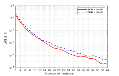
Figure 1: LHS of (14) versus the number of iterations (Algorithm 1).

In order to select the number of iterations for the cyclic procedures and EM algorithm, in Figure 1-2, we plot the left-hand side (LHS) of (14), (26), (32), and (33) versus the number of iterations for $K=16$ and $\Delta=10$. The two curves reported in the figures are related to two different SNR values and are obtained by averaging over $10^{4}$ Monte Carlo trials. In Figure 1, we show the behavior of the stopping criterion given by (14) for Algorithm 1. Inspection of the figure highlights that a number of iterations greater than $15$ returns variations lower than $10^{-2}$. The next figure concerns the convergence of Algorithm 2. Specifically, Subfigure 2(a) considers the LHS of (26) where $\sigma$ is replaced with the aforementioned initial value. It can be observed that $20$ iterations are enough to appreciate a variation of the compressed likelihood less than $10^{-3}$. Now, we use this number of iterations to obtain an initial estimate of $m$, which is, then, used to analyze the LHS of (32). The resulting curve is plotted in Subfigure 2(b), where $20$ iterations provide a variation of about $10^{-2}$. Finally, the curves reported in the third subfigure refer to the cyclic procedure of Algorithm 2 with $N_{EM,m}=N_{EM,\sigma}=20$. The subfigure points out that a number of iterations greater than or equal to $15$ can represent a good compromise between computational complexity and convergence issues. In a nutshell, in the next illustrative examples, we assume $N_{co,1}=N_{co,2}=15$ and $N_{EM,m}=N_{EM,\sigma}=20$.

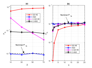
Figure 3: (a) Estimated $P_{fa}$ versus $\Delta$ assuming model (35); (b) Estimated $P_{fa}$ versus $q$; $K=16$ and thresholds computed under white noise hypothesis to ensure $P_{fa}=10^{-2}$.

In Figure 3(a), we estimate the $P_{fa}$ for the proposed detectors as a function of $\Delta$ (heterogeneity level) when the detection thresholds are computed assuming homogeneous white noise with power $\sigma^{2}_{n}$, $K=16$, and a nominal $P_{fa}=10^{-2}$. As expected, the AGD ensures the CFAR property since the estimated $P_{fa}$ is insensitive to the variations of $\Delta$ and is almost completely overlapped on the nominal $P_{fa}$. As for the remaining detectors, the GD-HE exhibits a resulting $P_{fa}$ which is almost two orders of magnitude higher than the nominal value ($10^{-2}$), whereas the $P_{fa}$ of C-AGD is close to $10^{-1}$. Finally, the $P_{fa}$ curve related to C-GD-HE experiences a decreasing behavior. In Figure 3(b), we estimate the $P_{fa}$ assuming a specific distribution for the interference power, i.e., data are modeled as compound-Gaussian random variables [41, 42], namely $x_{k}=\sqrt{\tau_{k}}g_{k}$, $k=1,\ldots,K$, where $g_{k}\sim\mbox{$\mathcal{C}$}\mbox{$\mathcal{N}$}_{1}(0,2\sigma^{2}_{n})$ and $\tau_{k}$, $k=1,\ldots,K$, follows the Gamma distribution whose pdf is $f(\tau_{k})=\frac{\displaystyle\tau_{k}^{b-1}}{\displaystyle\beta^{q}\Gamma(q)}\exp\{-\tau_{k}/\beta\}$ with $q>0$ and $\beta$ being the shape and scale parameters, respectively. The considered setting assumes $q=1/\beta$ to have a Gamma distribution with unit mean. Observe that for large values of $q$, data distribution approaches the Gaussian distribution. The Figure highlights that the $P_{fa}$ of the GD-HE, C-GD-HE, and C-AGD depends on the shape parameter $q$. Specifically, for low values of $q$, the estimated $P_{fa}$ significantly deviates from the nominal value On the other hand, as $q$ increases, the environment tends to be homogeneous and, hence, the $P_{fa}$ of GD-HE, C-GD-HE, and C-AGD approaches the nominal value $10^{-2}$. As for the AGD, the estimated $P_{fa}$ is very close to the nominal $P_{fa}$ regardless of the shape parameter value.

Summarizing, this analysis has corroborated that the AGD can ensure the CFAR property with respect to the power level of the interference in heterogeneous environments. On the contrary, the GD-HE, C-GD-HE, and C-AGD are not capable of maintain the false alarm rate constant. The last behavior can be explained by observing that the use of original data for estimation and/or detection does not allow to get rid of the dependence on the interference power at least for the aforementioned decision schemes, whereas the AGD takes advantage of the Invariance Principle to preserve the $P_{fa}$. Therefore, the GD-HE, C-GD-HE, and C-AGD do not exhibit usage flexibility; they could be possibly exploited in conjunction with a clutter map and a lookup table for the detection threshold selection.

Now, we focus on the detection performance of the devised architectures assuming model (35) and $P_{fa}=10^{-2}$; the Signal-to-Noise Ratio (SNR) is defined as $\mbox{SNR}=\|{\mbox{\boldmath$m$}}\|^{2}/\sigma^{2}_{n}$. For comparison purposes, we also report the $P_{d}$ curves of the Clairvoyant Detector (CD) based upon the LRT, whose expression is

$$-\sum_{k=1}^{K}\frac{\|{\mbox{\boldmath$x$}}_{k}-{\mbox{\boldmath$m$}}\|^{2}}{\sigma^{2}_{k}}+\sum_{k=1}^{K}\frac{\|{\mbox{\boldmath$x$}}_{k}\|^{2}}{\sigma^{2}_{k}}\mbox{$\begin{array}[]{c}\stackrel{{\scriptstyle\stackrel{{\scriptstyle\textstyle H_{1}}}{{\textstyle>}}}}{{\stackrel{{\scriptstyle\textstyle<}}{{\textstyle H_{0}}}}}\end{array}$}\eta,$$ (36)

the noncoherent linear detector or Energy Detector (ED) and the coherent detector (CHD), whose expressions are

$$\sum_{k=1}^{K}\|{\mbox{\boldmath$x$}}_{k}\|^{2}\mbox{$\begin{array}[]{c}\stackrel{{\scriptstyle\stackrel{{\scriptstyle\textstyle H_{1}}}{{\textstyle>}}}}{{\stackrel{{\scriptstyle\textstyle<}}{{\textstyle H_{0}}}}}\end{array}$}\eta\quad\mbox{and}\quad\left\|\sum_{k=1}^{K}{\mbox{\boldmath$x$}}_{k}\right\|^{2}\mbox{$\begin{array}[]{c}\stackrel{{\scriptstyle\stackrel{{\scriptstyle\textstyle H_{1}}}{{\textstyle>}}}}{{\stackrel{{\scriptstyle\textstyle<}}{{\textstyle H_{0}}}}}\end{array}$}\eta,$$ (37)

respectively.

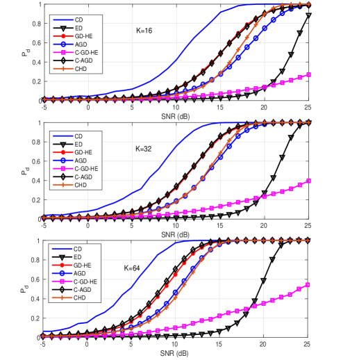
Figure 4: $P_{d}$ versus SNR for the CD, ED, GD-HE, AGD, C-GD-HE, C-AGD, and CHD assuming $\Delta=10$ and $P_{fa}=10^{-2}$.

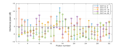
Figure 7: Power variation over the pulse burst for some range bins.

In Figure 4, we plot the $P_{d}$ curves for $\Delta=10$ and different values of $K$. The value of $\Delta$ corresponds to a moderate heterogeneity level and leads to a CNR of about $9$ dB. From inspection of the subfigures it turns out that the GD-HE and C-AGD exhibit better detection performances than the AGD, ED, CHD, and C-GD-HE. The latter is not capable to achieve $P_{d}=1$ for the considered parameter setting and its $P_{d}$ curves intersect those of ED. The loss of the ED with respect to the AGD at $P_{d}=0.9$ increases from about $4.5$ dB for $K=16$ to about $8$ dB when $K=64$. The curves of the CHD are in between those of the GD-HE and of the AGD with a gain over the latter that decreases as $K$ increases (note that for $K=32,64$ the considered curves are very close to each other). Moreover, the GD-HE and C-AGD experience a gain in between $1.5$ dB (for $K=16$) and $2$ dB (for $K=64$) over the AGD (at $P_{d}=0.9$). This hierarchy can be explained by the fact that the AGD is built up over normalized data and, hence, does not exploit all the available information with an avoidable performance degradation due to a lower estimation quality. However, such information loss allows to gain the CFAR property as shown in the previous figures. On the contrary, the GD-HE and C-AGD take advantage of all the available information but, as already highlighted, they do not guarantee the CFARness, which is of primary concern in radar. In the next figure, we compare the performances of the considered detectors assuming the same parameters as the previous figures but for $\Delta=50$, which leads to a more severe level of heterogeneity with respect to the previous examples, since now the CNR increases to about $23$ dB. Fluctuations of this order of magnitude can be observed in Figure 7 where clutter power variations over the time for live-recorded data are shown.

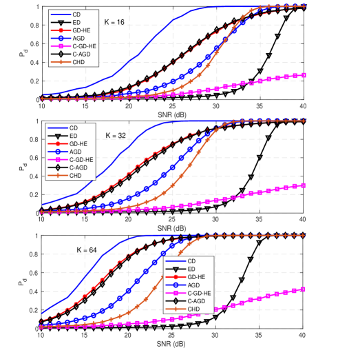
Figure 5: $P_{d}$ versus SNR for the CD, ED, GD-HE, AGD, C-GD-HE, C-AGD, and CHD assuming $\Delta=50$ and $P_{fa}=10^{-2}$.

Figure 5 confirms the behavior observed in Figure 4 with the difference that there exists an intersection between the $P_{d}$ curves of the GD-HE (and C-AGD) with those of the AGD and CHD in the high SNR region, where the latter slightly outperform the former. Moreover, the curves of the AGD and CHD intersect each other and the intersection point moves towards high SNR values as $K$ grows leading to a situation where the AGD outperforms the CHD with a gain of about $2$ dB at $P_{d}=0.9$ for $K=64$. The ED detector provides poor performances with a loss at $P_{d}=0.9$ with respect to the AGD that increases to about $10$ dB for $K=64$, whereas, for the considered simulating scenario, the maximum $P_{d}$ value achieved by the C-GD-HE is $0.4$ for $K=64$.

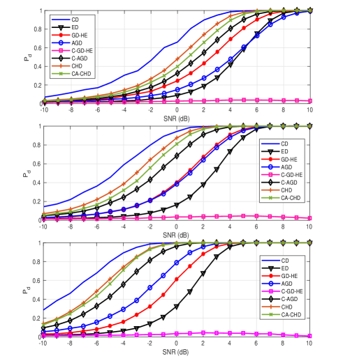
Figure 6: $P_{d}$ versus SNR for the CD, ED, GD-HE, AGD, C-GD-HE, C-AGD, CHD, and CA-CHD assuming $\Delta=0$ (homogeneous environment) and $P_{fa}=10^{-2}$.

For completeness, in Figure 6, we show the performance of the new architectures when $\Delta=0$, namely under the homogeneous environment. The curves of the cell-averaged coherent detector (CA-CHD), whose statistic is $\|\sum_{k=1}^{K}{\mbox{\boldmath$x$}}_{k}\|^{2}/\sum_{k=1}^{K}\|{\mbox{\boldmath$x$}}_{k}\|^{2}$, are also reported. In this case, the CHD followed by the CA-CHD overcome the other detectors (except for the CD) with the CHD gaining about $0.5$ dB with respect to the CA-CHD (the loss of the latter is due to the CFAR behavior [7]). The AGD shares almost the same performance as the ED for $K=16$, but as $K$ becomes larger and larger, the related $P_{d}$ curves improve. In fact, for $K=64$ and $P_{d}=0.9$, the AGD exhibits a loss of about $2$ dB with respect to the C-AGD and a gain of more than $1$ dB over the GD-HE.

Thus, the analysis on simulated data has singled out the AGD as an effective means to deal with heterogeneous data, since it ensures reasonable detection performances and, at the same time, retains the CFAR property, which is of primary importance in radar.

IV-B Real Data

In this section, we present numerical examples based upon live recorded data. To this end, we use the measurements which have been recorded in winter 1998 using the McMaster IPIX radar in Grimsby, on the shore of Lake Ontario, between Toronto and Niagara Falls. Specifically, we test the proposed algorithm on dataset 85 for the HH polarization and in order to meet the requirement on the noise power lower bound, we add $1$ to data. A detailed statistical analysis of the adopted real data has been conducted in [43].

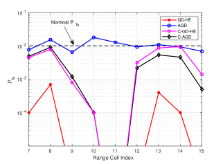
Figure 8: $P_{fa}$ estimated from the $7$th to the $15$th range bin for AGD and GD-HE over IPIX data assuming $K=16$ and thresholds computed under white noise hypothesis to ensure $P_{fa}=10^{-2}$.

The first analysis focuses on the CFARness and consists in estimating the $P_{fa}$ when the thresholds have been set under the white noise assumption with $C_{0}=1$. Specifically, the nominal $P_{fa}$ is set to $10^{-2}$ and heterogeneous data are selected using a sliding mechanism to generate $100/P_{fa}$ sets of possibly uncorrelated samples (high pulse repetition intervals). Before proceeding with the analysis, in Figure 7, we provide a glimpse of the data nature in terms of power variations for some pulse bursts. The figure highlighted the presence of significant power variations over the pulses confirming the heterogeneous nature of data (other sets not considered here for brevity experience an analogous behavior). The results of the CFAR analysis are shown in Figure 8. From the figure it turns out that the actual $P_{fa}$ of the AGD is very close to the nominal one confirming its CFAR behavior. On the other hand, the $P_{fa}$ of the remaining architectures considerably deviates from the nominal value. Specifically, the worst situation is experienced by the GD-HE, whose $P_{fa}$ values are always below $10^{-3}$. As for the C-AGD and C-GD-HE, they exhibit $P_{fa}$ values close to the nominal at a few range indices. It is also important to notice that for these architectures, the discrepancy with respect to the nominal $P_{fa}$ values can achieve several orders of magnitude with values outside the range considered in Figure 8.

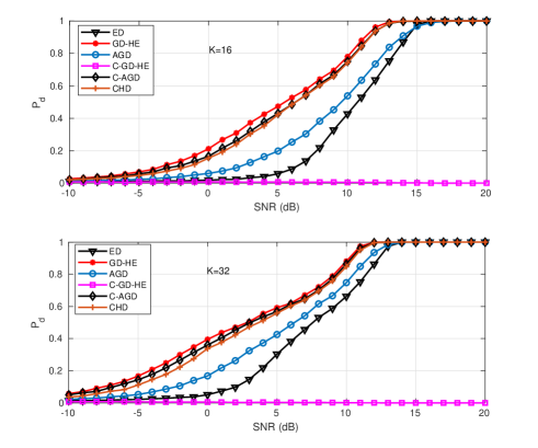
Figure 9: $P_{d}$ versus SNR for the ED, GD-HE, AGD, C-GD-HE, C-AGD, and CHD over IPIX data assuming $P_{fa}=10^{-2}$.

Finally, in Figure 9, we show the detection performance for different values of $K$ and for the $8$th range bin. In this case, all the considered decision schemes exploit a detection threshold ensuring the same $P_{fa}=10^{-2}$ and evaluated over the real data. The data set at each trial is obtained through a sliding window as described for the CFAR analysis. The figure is somehow reminiscent of the situation observed for synthetic data, where the GD-HE and C-AGD share the same performance confirming their superiority over the AGD with a gain that reduces to about $1$ dB for $K=32$. The main difference with respect to previous figures resides in the fact that the curves of the CHD are very close to those of the GD-HE and C-AGD. However, it is important to recall that such architectures do not provide a CFAR behavior and, hence, setting their thresholds in practical scenarios is not an easy task. Finally, the C-GD-HE continues to exhibit very poor performance at least for the considered parameter setting.

V Conclusions

In this paper, four new detection architectures for heterogeneous Gaussian environments have been proposed and assessed. Specifically, the first detector relies on original data and uses the likelihood ratio as decision statistic where the unknown target and interference parameters are estimated by means of a cyclic optimization procedure. The second decision scheme transfers data into the invariant domain and exploits normalized data, which are functionally invariant of scaling factors, to build up a CFAR decision scheme. Then, an alternating procedure incorporating the EM-Algorithm is devised to estimate the unknown parameters in the invariant domain. The remaining architectures have been obtained by combining the estimation procedure for the original data domain with the detector for the invariant data domain and vice versa. The behavior of these architectures has been first investigated resorting to simulated data adhering the design assumptions and, then, they have been tested on real recorded data. The analysis has singled out the second decision scheme based upon normalized data as the recommended solution for adaptive detection in heterogeneous environments since it can guarantee the CFAR property and a limited detetion loss with respect to the other architectures which exploit estimates based upon all the available information carried by data and whose $P_{fa}$ is very sensitive to the interference power variations.

Finally, it would be of interest investigating the behavior of the proposed architectures in the presence of a mismatch for the noise power lower bound as well as extending the herein presented approach to the case of coherent processing through space-time data vectors sharing the same structure of the interference covariance matrix but different power levels.

Appendix A Maximal Invariant Statistic for Scaling Transformations

In this appendix, we prove that (5) is a MIS with respect to $\mathcal{G}$. To this end, we recall that ${\mbox{\boldmath$T$}}(\cdot,\ldots,\cdot)$ is said to be a MIS if and only if

$$\begin{cases}{\mbox{\boldmath$T$}}({\mbox{\boldmath$x$}}_{1},\ldots,{\mbox{\boldmath$x$}}_{K})={\mbox{\boldmath$T$}}({\mbox{\boldmath$G$}}({\mbox{\boldmath$x$}}_{1},\ldots,{\mbox{\boldmath$x$}}_{K})),\quad\forall{\mbox{\boldmath$G$}}\in\mbox{$\mathcal{G}$}\,;\\ \begin{aligned} {\mbox{\boldmath$T$}}({\mbox{\boldmath$x$}}_{1},&\ldots,{\mbox{\boldmath$x$}}_{K})={\mbox{\boldmath$T$}}(\bar{{\mbox{\boldmath$x$}}}_{1},\ldots,\bar{{\mbox{\boldmath$x$}}}_{K})\Rightarrow\\ &\exists\,\bar{{\mbox{\boldmath$G$}}}\in\mbox{$\mathcal{G}$}\,:\,[{\mbox{\boldmath$x$}}_{1},\ldots,{\mbox{\boldmath$x$}}_{K}]=\bar{{\mbox{\boldmath$G$}}}[\bar{{\mbox{\boldmath$x$}}}_{1},\ldots,\bar{{\mbox{\boldmath$x$}}}_{K}]\,.\end{aligned}\end{cases}$$ (38)

The first property is evident since ${\mbox{\boldmath$T$}}\left({\mbox{\boldmath$c$}}(1){\mbox{\boldmath$x$}}_{1},\ldots,{\mbox{\boldmath$c$}}(K){\mbox{\boldmath$x$}}_{K}\right)={\mbox{\boldmath$T$}}\left({\mbox{\boldmath$x$}}_{1},\ldots,{\mbox{\boldmath$x$}}_{K}\right)$, $\forall{\mbox{\boldmath$c$}}\in{\mathds{R}}_{+}^{K\times 1}$. To prove the maximality, assume that ${\mbox{\boldmath$T$}}({\mbox{\boldmath$x$}}_{1},\ldots,{\mbox{\boldmath$x$}}_{K})={\mbox{\boldmath$T$}}(\bar{{\mbox{\boldmath$x$}}}_{1},\ldots,\bar{{\mbox{\boldmath$x$}}}_{K})$ and let $\bar{{\mbox{\boldmath$c$}}}=\left[\frac{\|{\mbox{\boldmath$x$}}_{1}\|}{\|\bar{{\mbox{\boldmath$x$}}}_{1}\|},\ldots,\frac{\|{\mbox{\boldmath$x$}}_{K}\|}{\|\bar{{\mbox{\boldmath$x$}}}_{K}\|}\right]^{T}\in{\mathds{R}}_{+}^{K\times 1}$. It follows that we can define the action $\bar{{\mbox{\boldmath$G$}}}(\bar{{\mbox{\boldmath$x$}}}_{1},\ldots,\bar{{\mbox{\boldmath$x$}}}_{K})=[\bar{{\mbox{\boldmath$c$}}}(1)\bar{{\mbox{\boldmath$x$}}}_{1},\ldots,\bar{{\mbox{\boldmath$c$}}}(K)\bar{{\mbox{\boldmath$x$}}}_{K}]=[{\mbox{\boldmath$x$}}_{1},\ldots,{\mbox{\boldmath$x$}}_{K}]$. Thus, we have found $\bar{{\mbox{\boldmath$G$}}}\in\mbox{$\mathcal{G}$}$ which meets the second requirement of (38) and the proof is complete.

Appendix B Derivation of (7)

Let us start the derivation by writing (3.5.48) of [32] with ${\mbox{\boldmath$\Sigma$}}=\sigma^{2}_{i}{\mbox{\boldmath$I$}}$, namely

$$f_{1}({\mbox{\boldmath$z$}}_{i};{\mbox{\boldmath$m$}},\sigma_{i}) =\frac{1}{2\pi}\exp\left\{\frac{-\|{\mbox{\boldmath$m$}}\|^{2}}{(2\sigma^{2}_{i})}\right\}+\frac{{\mbox{\boldmath$z$}}_{i}^{T}{\mbox{\boldmath$m$}}}{\sigma_{i}}\Phi\left(\frac{{\mbox{\boldmath$z$}}_{i}^{T}{\mbox{\boldmath$m$}}}{\sigma_{i}}\right)$$

$$\times\frac{1}{\sqrt{2\pi}}\exp\left\{-\frac{(m_{1}z_{i,2}-m_{2}z_{i,1})^{2}}{2\sigma^{2}_{i}}\right\},$$ (39)

where ${\mbox{\boldmath$m$}}=[m_{1}\ m_{2}]^{T}$ and ${\mbox{\boldmath$z$}}_{i}=[z_{i,1}\ z_{i,2}]^{T}$. Now, observe that

$$(m_{1}z_{i,2}-m_{2}z_{i,1})^{2}=m_{1}^{2}z_{i,2}^{2}+m_{2}^{2}z_{i,1}^{2}-2m_{1}m_{2}z_{i,1}z_{i,2}$$

$$=m_{1}^{2}z_{i,2}^{2}+m_{2}^{2}z_{i,1}^{2}-2m_{1}m_{2}z_{i,1}z_{i,2}+({\mbox{\boldmath$z$}}_{i}^{T}{\mbox{\boldmath$m$}})^{2}-({\mbox{\boldmath$z$}}_{i}^{T}{\mbox{\boldmath$m$}})^{2}$$

$$=m_{1}^{2}z_{i,2}^{2}+m_{2}^{2}z_{i,1}^{2}+m_{1}^{2}z_{i,1}^{2}+m_{2}^{2}z_{i,2}^{2}-({\mbox{\boldmath$z$}}_{i}^{T}{\mbox{\boldmath$m$}})^{2}$$

$$=\|{\mbox{\boldmath$m$}}\|^{2}-({\mbox{\boldmath$z$}}_{i}^{T}{\mbox{\boldmath$m$}})^{2}.$$ (40)

Replacing the above result in (39), we obtain (7) and the proof is concluded.

Appendix C Expression of $\xi(p)$

Focus on the logarithm argument of (22) and rewrite it as

$$\int_{0}^{+\infty}\!\!\!\!\!\!\exp\{t(x_{k})p_{k}\}h(x_{k})dx_{k}=\int_{0}^{+\infty}\!\!\!\!\!\!\exp\left\{\frac{x_{k}}{\sigma^{2}_{k}}p_{k}-\frac{x_{k}^{2}}{2\sigma^{2}_{k}}\right\}x_{k}dx_{k}$$

$$=\exp\left\{\frac{p_{k}^{2}}{2\sigma^{2}_{k}}\right\}\int_{0}^{+\infty}\exp\left\{-\frac{(x_{k}-p_{k})^{2}}{2\sigma^{2}_{k}}\right\}x_{k}dx_{k}$$

$$=-\exp\left\{\frac{p_{k}^{2}}{2\sigma^{2}_{k}}\right\}\sigma^{2}_{k}\int_{0}^{+\infty}\frac{{(p_{k}-x_{k})}/{\sigma^{2}_{k}}}{\exp\left\{{(x_{k}-p_{k})^{2}}/{2\sigma^{2}_{k}}\right\}}dx_{k}$$

$$+p_{k}\frac{\displaystyle\int_{0}^{+\infty}\exp\left\{-\frac{(x_{k}-p_{k})^{2}}{2\sigma^{2}_{k}}\right\}dx_{k}}{\exp\left\{\displaystyle-{p_{k}^{2}}/{2\sigma^{2}_{k}}\right\}}=\sigma^{2}_{k}+\sigma_{k}p_{k}\frac{\Phi(p_{k}/\sigma_{k})}{\varphi(p_{k}/\sigma_{k})},$$

where the last equality concludes the proof.

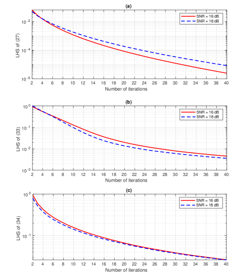
Figure 2: Convergence curves for Algorithm 2: LHS of (26) versus the number of iterations (a); LHS of (32) versus the number of iterations (b); LHS of (33) versus the number of iterations (c).

Algorithm 1 Iterative estimation of $m$ and ${\mbox{\boldmath$\sigma$}}^{2}$ in the original domain

0:  $C_{0}$, $N_{co,1}$, $\epsilon$, $X$, and $({\mbox{\boldmath$\sigma$}}^{2})^{(0)}$.

0:  $\widehat{{\mbox{\boldmath$m$}}}^{(n)}$ and $(\widehat{{\mbox{\boldmath$\sigma$}}}^{2}_{1})^{(n)}$.

1:  Set $n=0$

2:  Set $n=n+1$

3:  Compute $\widehat{{\mbox{\boldmath$m$}}}^{(n)}=\left[\sum_{k=1}^{K}\frac{1}{(\sigma_{k}^{2})^{(n-1)}}\right]^{-1}\sum_{k=1}^{K}\frac{{\bf x}_{k}}{(\sigma_{k}^{2})^{(n-1)}}$

4:  Compute $(\widehat{{\mbox{\boldmath$\sigma$}}}^{2}_{1})^{(n)}=[\max\{\frac{1}{2}\|{\mbox{\boldmath$x$}}_{1}-\widehat{{\mbox{\boldmath$m$}}}^{(n)}\|^{2},C_{0}\},\ldots,\max\{\frac{1}{2}\|{\mbox{\boldmath$x$}}_{K}-\widehat{{\mbox{\boldmath$m$}}}^{(n)}\|^{2},C_{0}\}]^{T}$

5:  If the stopping criterion is not satisfied go to step 2 else go to step 6

6:  Return $\widehat{{\mbox{\boldmath$m$}}}^{(n)}$ and $(\widehat{{\mbox{\boldmath$\sigma$}}}^{2}_{1})^{(n)}$

Algorithm 2 Iterative estimation of $m$ and ${\mbox{\boldmath$\sigma$}}^{2}$ in the invariant domain

0:  $N_{EM,m}$, $N_{EM,\sigma}$, $N_{co,2}$, $C_{0}$, $\epsilon_{1}$, $\epsilon_{2}$, $\epsilon_{3}$, ${\mbox{\boldmath$z$}}_{k}$, $k=1,\ldots,K$, $\widehat{{\mbox{\boldmath$m$}}}^{(0),(0)}$, and $(\tilde{{\mbox{\boldmath$\sigma$}}}^{2})^{(0),(0)}$.

0:  $\widehat{{\mbox{\boldmath$m$}}}$ and $\tilde{{\mbox{\boldmath$\sigma$}}}$.

1:  Set $i=0$ and $\bar{{\mbox{\boldmath$\sigma$}}}^{2}=(\tilde{{\mbox{\boldmath$\sigma$}}}^{2})^{(0),(0)}$

2:  Set $n=0$

3:  Compute $\forall k=1,\ldots,K$, $h_{k}^{(n)}=E[b_{k}|{\mbox{\boldmath$z$}}_{k};\widehat{{\mbox{\boldmath$m$}}}^{(n),(i)},\bar{{\mbox{\boldmath$\sigma$}}}^{2}]$ using (24) and ${\mbox{\boldmath$H$}}^{(n)}=\mbox{\boldmath\bf diag}\,(h_{1}^{(n)},\ldots,h_{K}^{(n)})$

4:  Compute $\widehat{{\mbox{\boldmath$m$}}}^{(n+1),(i)}$ using (25)

5:  Set $n=n+1$

6:  if the stopping criterion for the EM-Algorithm is satisfied go to step 7 else go to step 3

7:  Set $\bar{{\mbox{\boldmath$m$}}}={\mbox{\boldmath$m$}}^{(n),(i)}$

8:  Set $n=0$ and $\bar{p}_{k}={\mbox{\boldmath$z$}}_{k}^{T}\bar{{\mbox{\boldmath$m$}}}$

9:  Compute $(\tilde{\sigma}^{2}_{k})^{(n+1),(i)}$ using (31) and set $(\widehat{\sigma}^{2}_{k})^{(n+1),(i)}=\max\{(\tilde{\sigma}^{2}_{k})^{(n+1),(i)},C_{0}\}$

10:  Set $n=n+1$

11:  if the stopping criterion for the EM-Algorithm is satisfied set $i=i+1$ and go to step 12 else go to step 9

12:  if the stopping criterion for the cyclic procedure is not satisfied set ${\mbox{\boldmath$m$}}^{(0),(i)}=\bar{{\mbox{\boldmath$m$}}}$, $\bar{{\mbox{\boldmath$\sigma$}}}^{2}=[(\widehat{\sigma}^{2}_{1})^{(n),(i)},\ldots,(\widehat{\sigma}^{2}_{K})^{(n),(i)}]^{T}$, and go to step 2, else return $\widehat{{\mbox{\boldmath$m$}}}=\bar{{\mbox{\boldmath$m$}}}$ and $\widehat{{\mbox{\boldmath$\sigma$}}}^{2}=[(\widehat{\sigma}_{1}^{2})^{(n),(i)},\ldots,(\widehat{\sigma}_{K}^{2})^{(n),(i)}]^{T}$

References

- [1] E. J. Kelly, “An adaptive detection algorithm,” IEEE Transactions on Aerospace and Electronic Systems, no. 2, pp. 115–127, 1986.
- [2] F. C. Robey, D. R. Fuhrmann, E. J. Kelly, and R. Nitzberg, “A CFAR adaptive matched filter detector,” IEEE Transactions on Aerospace and Electronic Systems, vol. 28, no. 1, pp. 208–216, 1992.
- [3] F. Bandiera, D. Orlando, and G. Ricci, Advanced Radar Detection Schemes Under Mismatched Signal Models, M. . C. P. Synthesis Lectures on Signal Processing No. 8, Ed., San Rafael, US, 2009.
- [4] J. Liu, W. Liu, B. Chen, H. Liu, H. Li, and C. Hao, “Modified Rao Test for Multichannel Adaptive Signal Detection,” IEEE Transactions on Signal Processing, vol. 64, no. 3, pp. 714–725, 2016.
- [5] C. Hao, S. Gazor, G. Foglia, B. Liu, and C. Hou, “Persymmetric adaptive detection and range estimation of a small target,” IEEE Transactions on Aerospace and Electronic Systems, vol. 51, no. 4, pp. 2590–2604, 2015.
- [6] C. Hao, D. Orlando, G. Foglia, and G. Giunta, “Knowledge-based adaptive detection: Joint exploitation of clutter and system symmetry properties,” IEEE Signal Processing Letters, vol. 23, no. 10, pp. 1489–1493, October 2016.
- [7] M. A. Richards, J. A. Scheer, and W. A. Holm, Principles of Modern Radar: Basic Principles. Raleigh, NC: Scitech Publishing, 2010.
- [8] F. Bandiera, O. Besson, D. Orlando, G. Ricci, and L. L. Scharf, “GLRT-Based Direction Detectors in Homogeneous Noise and Subspace Interference,” IEEE Transactions on Signal Processing, vol. 55, no. 6, pp. 2386–2394, June 2007.
- [9] D. Ciuonzo, A. De Maio, and D. Orlando, “A unifying framework for adaptive radar detection in homogeneous plus structured interference-part ii: Detectors design,” IEEE Transactions on Signal Processing, vol. 64, no. 11, pp. 2907–2919, June 2016.
- [10] R. S. Raghavan, N. Pulsone, and D. J. McLaughlin, “Performance of the GLRT for adaptive vector subspace detection,” IEEE Transactions on Aerospace and Electronic Systems, vol. 32, no. 4, pp. 1473–1487, October 1996.
- [11] I. S. Reed, J. D. Mallett, and L. E. Brennan, “Rapid convergence rate in adaptive arrays,” IEEE Transactions on Aerospace and Electronic Systems, no. 6, pp. 853–863, 1974.
- [12] W. L. Melvin, “Space-time adaptive radar performance in heterogeneous clutter,” IEEE Transactions on Aerospace and Electronic Systems, vol. 36, no. 2, pp. 621–633, 2000.
- [13] J. S. Bergin, P. M. Techau, W. L. Melvin, and J. R. Guerci, “GMTI STAP in target-rich environments: site-specific analysis,” in Radar Conference, 2002. Proceedings of the IEEE. IEEE, 2002, pp. 391–396.
- [14] P. Wang, H. Li, and B. Himed, “Knowledge-aided parametric tests for multichannel adaptive signal detection,” IEEE Transactions on Signal Processing, vol. 59, no. 12, pp. 5970–5982, 2011.
- [15] A. De Maio, A. Farina, and G. Foglia, “Knowledge-aided bayesian radar detectors & their application to live data,” IEEE Transactions on Aerospace and Electronic Systems, vol. 46, no. 1, pp. 170–183, 2010.
- [16] Y. I. Abramovich and B. A. Johnson, “Glrt-based detection-estimation for undersampled training conditions,” IEEE Transactions on Signal Processing, vol. 56, no. 8, pp. 3600–3612, Aug 2008.
- [17] Y. I. Abramovich and O. Besson, “On the Expected Likelihood Approach for Assessment of Regularization Covariance Matrix,” IEEE Signal Processing Letters, vol. 22, no. 6, pp. 777–781, June 2015.
- [18] Y. Chen, A. Wiesel, and A. O. Hero, “Robust shrinkage estimation of high-dimensional covariance matrices,” IEEE Transactions on Signal Processing, vol. 59, no. 9, pp. 4097–4107, Sep. 2011.
- [19] E. Ollila and D. E. Tyler, “Regularized-estimators of scatter matrix,” IEEE Transactions on Signal Processing, vol. 62, no. 22, pp. 6059–6070, Nov 2014.
- [20] Y. I. Abramovich, N. K. Spencer, and A. Y. Gorokhov, “Modified glrt and amf framework for adaptive detectors,” IEEE Transactions on Aerospace and Electronic Systems, vol. 43, no. 3, pp. 1017–1051, July 2007.
- [21] M. J. Steiner and K. Gerlach, “Fast converging adaptive processor or a structured covariance matrix,” IEEE Transactions on Aerospace and Electronic Systems, vol. 36, no. 4, pp. 1115–1126, Oct 2000.
- [22] M. C. Wicks, W. L. Melvin, and P. Chen, “An efficient architecture for nonhomogeneity detection in space-time adaptive processing airborne early warning radar,” in Radar 97 (Conf. Publ. No. 449), Oct 1997, pp. 295–299.
- [23] M. Rangaswamy, “Non-homogeneity detector for gaussian and non-gaussian interference scenarios,” in Sensor Array and Multichannel Signal Processing Workshop Proceedings, 2002, Aug 2002, pp. 528–532.
- [24] R. S. Adve, T. B. Hale, and M. C. Wicks, “Transform domain localized processing using measured steering vectors and non-homogeneity detection,” in Proceedings of the 1999 IEEE Radar Conference. Radar into the Next Millennium (Cat. No.99CH36249), April 1999, pp. 285–290.
- [25] L. Jiang and T. Wang, “Robust non-homogeneity detector based on reweighted adaptive power residue,” IET Radar, Sonar Navigation, vol. 10, no. 8, pp. 1367–1374, 2016.
- [26] B. Himed, Y. Salama, and J. H. Michels, “Improved detection of close proximity targets using two-step nhd,” in Record of the IEEE 2000 International Radar Conference [Cat. No. 00CH37037], May 2000, pp. 781–786.
- [27] M. Rangaswamy, “Statistical analysis of the nonhomogeneity detector for non-gaussian interference backgrounds,” IEEE Transactions on Signal Processing, vol. 53, no. 6, pp. 2101–2111, June 2005.
- [28] S. Kraut and L. L. Scharf, “The CFAR adaptive subspace detector is a scale-invariant GLRT,” IEEE Transactions on Signal Processing, vol. 47, no. 9, pp. 2538–2541, 1999.
- [29] J. Ward, “Space-time adaptive processing for airborne radar,” MIT Lincoln Laboratory, Tech. Rep. 1015, 1994.
- [30] A. Papoulis and S. Pillai, Probability, Random Variables, and Stochastic Processes. McGraw-Hill, 2002.
- [31] E. L. Lehmann, Testing Statistical Hypotheses, 2nd ed. New York, USA: Springer-Verlag, 1986.
- [32] K. V. Mardia and P. E. Jupp, Directional Statistics. John Wiley & Sons, 2000.
- [33] A. P. Dempster, N. M. Laird, and D. B. Rubin, “Maximum likelihood from incomplete data via the EM algorithm,” Journal of the Royal Statistical Society (Series B - Methodological), vol. 39, no. 1, pp. 1–38, 1977.
- [34] S. Haykin, R. Bakker, and B. W. Currie, “Uncovering nonlinear dynamics-the case study of sea clutter,” Proceedings of the IEEE, vol. 90, no. 5, pp. 860–881, 2002.
- [35] A. Farina, Antenna-Based Signal Processing Techniques for Radar Systems, A. House, Ed., Boston, MA, 1992.
- [36] P. Stoica and Y. Selen, “Cyclic minimizers, majorization techniques, and the expectation-maximization algorithm: a refresher,” IEEE Signal Processing Magazine, vol. 21, no. 1, pp. 112–114, 2004.
- [37] L. Scharf and C. Demeure, Statistical Signal Processing: Detection, Estimation, and Time Series Analysis, ser. Addison-Wesley series in electrical and computer engineering. Addison-Wesley Publishing Company, 1991.
- [38] J. Shao, Mathematical Statistics, ser. Springer Texts in Statistics. Springer New York, 2008.
- [39] L. D. Brown, “Fundamentals of statistical exponential families with applications in statistical decision theory,” Lecture Notes-Monograph Series, vol. 9, pp. i–279, 1986.
- [40] C. N. Morris, “Natural exponential families with quadratic variance functions: Statistical theory,” The Annals of Statistics, vol. 11, no. 2, pp. 515–529, 1983.
- [41] E. Conte, M. Lops, and G. Ricci, “Adaptive detection schemes in compound-Gaussian clutter,” IEEE Transactions on Aerospace and Electronic Systems, vol. 34, no. 4, pp. 1058–1069, 1998.
- [42] F. Gini and A. Farina, “Vector Subspace Detection in Compound-Gaussian Clutter Part I: Survey and New Results,” IEEE Transactions on Aerospace and Electronic Systems, vol. 38, no. 4, pp. 1295–1311, 2002.
- [43] E. Conte, A. De Maio, and C. Galdi, “Statistical analysis of real clutter at different range resolutions,” IEEE Transactions on Aerospace and Electronic Systems, vol. 40, no. 3, pp. 903–918, 2004.