Exact Solutions Of Time Fractional Generalized Burgers-Fisher Equation Using Exp function and Exponential Rational Function Methods

Abstract

Using modified Riemann-Liouville derivative, the Exp function and Exponential rational function methods are implemented to solve the time fractional generalized Burgers-Fisher equation (TF-GBF). The TF-GBF is transformed into a nonlinear ordinary differential equation (NLODE) by applying the transformation of traveling wave. The suggested methods are then introduced to formulate exact solutions for the resulting equation. The solutions are depicted using 2D and 3D plots.

Keywords: Fractional derivative; Time fractional generalized Burgers-Fisher equation; Exp function method; Exponential rational function method

1 Introduction

In the year 1695, Leibnitz introduced a fractional calculus. Several studies have been carried out on science and engineering related to fractional phenomena such as plasma physics, viscoelastic materials, fluid flow, biology, economics, probability and statistics, polymers, optical fibers, etc. In recent years, fractional differential equations (FDEs) have gained a considerable popularity among scientists and engineers and finding solutions for nonlinear FDE (NLFDE) is an indefatigable research field [1, 2, 3, 4, 5, 6].

Numerous mathematical procedures have been developed and investigated to find the exact solutions of the NLFDE. For instance, the sine-cosine method [7, 8], the tanh method [9], Adomian decomposition method [10], the sub-equation method [11, 12], variational iteration method [13], the first integral method [14, 15] and so on [16, 17, 18]. Recently, an Exp-function method, which was proposed by He and Wu [19] and consistently studied in [20, 21, 22]. This method was previously suggested for evaluating a solution for PDEs. In addition, it was expanded successfully to FDEs [23, 24, 25, 26, 27].

In addition, the exponential rational function method (ERFM) is one of the methods to reveal the exact solutions. At first, it was originated by [28]. Furthermore, it has been executed in many fields of engineering and science [29, 30, 31]. From the contribution of the prior mentioned schemes, we carry out this analysis to the time fractional generalized Burgers-Fisher equation (TF-GBFE). A nonlinear equation is called the Burgers-Fisher equation and is the combination of reaction, convection and diffusion process. The properties of the convective phenomenon of Burgers and Fisher’s diffusion transport as well as reaction form characteristics are used in the nonlinear equation. The GBFE is used in the field of fluid dynamics. It was also found in some applications including gas dynamics, heat conduction, elasticity, etc.

The GBFE with the order of time fractional $\alpha$ and an arbitrary constants $\beta,\gamma$ and $\delta$ is given by

$$u^{\alpha}_{t}+\beta u^{\delta}u_{x}-u_{xx}=\gamma u(1-u^{\delta}),$$ (1)

where $\alpha\in(0,1]$.

The present work is classified as follows: Section 2 describes the properties of the modified Riemann-Liouville fractional derivative and the description and implementation of Exp function method in TF-GBFE is given in section 3. The description and implementation of ERFM in TF-GBFE is clarified in section 4. Section 5 presents the results and discussion of the proposed method for TF-GBFE and section 6 ends with conclusion.

2 The modified Riemann-Liouville (RL) derivative

Recent studies have shown that the dynamics of many physical processes are precisely described using FDEs with various types of fractional derivatives. Jumarie has given a different interpretation of the fractional derivative with a minor modification of the Riemann-Liouville (RL) derivative [32, 33] and it is defined as

$$D^{\alpha}_{t}g(t)=\left\{\begin{array}[]{ll}\displaystyle{\frac{1}{\Gamma(1-\alpha)}\frac{d}{dt}\int_{0}^{t}(t-\zeta)^{-\alpha-1}[g(\zeta)-g(0)]d\zeta},\;0<\alpha<1,\\ \displaystyle{(g^{(\vartheta)}(t))^{(\alpha-\vartheta)}},\vartheta\leq\alpha<\vartheta+1,\;\vartheta\geq 1,\end{array}\right.$$ (2)

where $\alpha$ denotes the order of fractional derivative and $g(t)$ denotes a continuous non differentiable function $g:\mathbb{R}\to\mathbb{R}$, $t\to g(t)$. Some notable properties of modified RL derivative are listed below [34, 35]:
Property: 1

$$D^{\alpha}_{t}t^{\kappa}=\frac{\Gamma(1+\kappa)}{\Gamma(1+\kappa-\alpha)}t^{\kappa-\alpha},\;\kappa>0.$$

Property: 2

$$D^{\alpha}_{t}(pg(t)+qh(t))=pD^{\alpha}_{t}g(t)+qD^{\alpha}_{t}h(t).$$

where $g$ and $h$ are constants.
Property: 3

$$D^{\alpha}_{t}k=0,\;k=constant.$$

For the following problem, these properties can be used.

3 The Exp Function Method

Let us consider the NLFDE with an unknown function $u$, the polynomial G of $u$ and its partial derivatives, involving the highest order derivatives and the nonlinear terms,

$$G(u,D^{\alpha}_{t}u,D^{\beta}_{x}u,D^{\alpha}_{t}D^{\alpha}_{t}u,D^{\alpha}_{t}D^{\beta}_{x}u,D^{\beta}_{x}D^{\beta}_{x}u,\ldots)=0,\;\;0<\alpha,\beta<1.$$ (3)

With the following fractional complex transform [35] with nonzero arbitrary constants $\lambda$ and $\xi$, we transform fractional differential equation into ordinary differential equation:

$$u(x,t)=u(\zeta),\;\zeta=\frac{\lambda t^{\alpha}}{\Gamma[1+\alpha]}+\frac{\xi x^{\beta}}{\Gamma[1+\beta]},$$ (4)

Reduce Eq.(3) to the following ordinary differential equation (ODE) of integer order:

$$H(u,u^{\prime},u^{\prime\prime},u^{\prime\prime\prime},\ldots)=0,$$ (5)

where prime denotes a derivative of $\zeta$.
With the positive integers $g,h,k,$ and $j$, also with the unknown constants $a_{q}$ and $b_{p}$, the Exp function can be expressed in the form:

$$u(\zeta)=\frac{\sum^{h}_{q=-g}a_{q}e^{q\zeta}}{\sum^{j}_{p=-k}b_{p}e^{p\zeta}}.$$ (6)

We may evaluate the values of $h,j$ and $g,k$ respectively by balancing the highest order and the lowest order within the Exp function.

3.1 Exp function for the time fractional generalized Burgers-Fisher equation

We apply the following transformation in order to solve the TF-GBFE using the proposed method:

$$u(x,t)=u(\zeta),\;\zeta=kx-\frac{\lambda t^{\alpha}}{\Gamma[1+\alpha]}$$ (7)

Now Eq.(7) in Eq.(1), we get

$$k^{2}u^{\prime\prime}+(\lambda-k\beta u^{\delta})u^{\prime}+\gamma u(1-u^{\delta})=0.$$ (8)

Applying the following folding transformation in Eq.(8)

$$u(\zeta)=v^{\frac{1}{\delta}}(\zeta),$$ (9)

we obtain the following NLODE:

$$k^{2}\delta vv^{\prime\prime}+k^{2}(1-\delta){v^{\prime}}^{2}+(\lambda-k\beta v)\delta v{v^{\prime}}+\gamma\delta^{2}(1-v)v^{2}=0.$$ (10)

According to Exp function method, we assume that the solution of Eq.(10) can be expressed in the form

$$u(\zeta)=\frac{\sum^{h}_{q=-g}a_{q}e^{q\zeta}}{\sum^{j}_{p=-k}b_{p}e^{p\zeta}}=\frac{a_{-g}e^{-g\zeta}+\dots+a_{k}e^{k\zeta}}{b_{-h}e^{-h\zeta}+\dots+b_{j}e^{j\zeta}}.$$ (11)

Balancing the highest order in Eq.(10) for $vv^{\prime\prime}$ and $v^{2}v^{\prime}$, we have

$$vv^{\prime\prime}=\frac{h_{5}e^{(2k+3j)\zeta+\dots}}{h_{6}e^{(5j)\zeta+\dots}}$$ (12)

and

$$v^{2}v^{\prime}=\frac{h_{9}e^{(3k+j)\zeta}+\dots}{h_{10}e^{(4j)\zeta}+\dots}=\frac{h_{9}e^{(3k+2j)\zeta}+\dots}{h_{10}e^{(5j)\zeta}+\dots}.$$ (13)

Balancing highest order of Exp function in Eq.(12) and Eq.(13), we obtain

$$2k+3j=3k+2j,\;\;k=j.$$ (14)

Likewise, balancing the lowest order in Eq.(10) for $vv^{\prime\prime}$ and $v^{2}v^{\prime}$, we have

$$vv^{\prime\prime}=\frac{a_{5}e^{-(2g+3h)\zeta}+\dots}{a_{6}e^{(-5h)\zeta}+\dots}$$ (15)

and

$$v^{2}v^{\prime}=\frac{a_{9}e^{-(3g+h)\zeta}+\dots}{a_{10}e^{(-4h)\zeta}+\dots}=\frac{a_{9}e^{-(3g+2h)\zeta}+\dots}{a_{10}e^{(-5h)\zeta}+\dots}.$$ (16)

Balancing lowest order of Exp function in Eq.(15) and Eq.(16), we obtain

$$2g+3h=3g+2h,\;\;g=h.$$ (17)

For the choices of $k=j=1$ and $g=h=1$, Eq.(11) becomes,

$$v(\zeta)=\frac{a_{1}e^{(\zeta)}+a_{0}+a_{-1}e^{(-\zeta)}}{b_{1}e^{(\zeta)}+b_{0}+b_{-1}e^{(-\zeta)}}.$$ (18)

Substituting Eq.(18) into Eq.(10), we obtain the following cases with different parametric choices of $a_{-1},a_{0},a_{1},b_{-1},b_{0}$ and $b_{1}$.
Case:1

$$a_{-1}=0,\;a_{0}=0,\;b_{-1}=0,\;b_{0}=0,\;\lambda=\frac{-k^{2}-\gamma\delta^{2}}{\delta},k=\frac{-\gamma\delta}{\beta},$$

Eq.(10) becomes

$$-\gamma\delta vv^{\prime\prime}-\beta^{2}v^{2}(1+v^{\prime})+\beta^{2}v^{3}+(\beta^{2}+\gamma)vv^{\prime}+\gamma(\delta-1)=0,$$ (19)

we obtain

$$v(x,t)=\frac{a_{1}e^{\big{(}{\frac{kx{\Gamma[1+\alpha]}-\lambda t^{\alpha}}{{\Gamma[1+\alpha]}}\big{)}}}}{b_{0}},$$ (20)

then the exact solution is

$$u(x,t)=\displaystyle\left[\frac{a_{1}e^{\big{(}{\frac{kx{\Gamma[1+\alpha]}-\lambda t^{\alpha}}{{\Gamma[1+\alpha]}}\big{)}}}}{b_{0}}\right]^{\frac{1}{\delta}}.$$ (21)

Case:2

$$a_{-1}=0,\;a_{0}=0,\;b_{-1}=0,\;a_{1}=b_{1},\;\gamma=\frac{2k^{2}}{\delta^{2}},\;\lambda=\frac{-4k^{2}-\gamma\delta^{2}}{2\delta},\;k=\frac{-\beta\delta}{1+\delta},$$

Eq.(10) becomes

$$\delta vv^{\prime\prime}+(2+(1+\delta)v^{\prime})v^{2}-(\delta-1){v^{\prime}}^{2}-3vv^{\prime}-2v^{3}=0,$$ (22)

we obtain

$$v(x,t)=\frac{a_{1}e^{\big{(}{\frac{kx{\Gamma[1+\alpha]}-\lambda t^{\alpha}}{{\Gamma[1+\alpha]}}\big{)}}}}{a_{1}e^{\big{(}{\frac{kx{\Gamma[1+\alpha]}-\lambda t^{\alpha}}{{\Gamma[1+\alpha]}}\big{)}}}+b_{0}},$$ (23)

then the exact solution is

$$u(x,t)=\displaystyle\left[\frac{a_{1}e^{\big{(}{\frac{kx{\Gamma[1+\alpha]}-\lambda t^{\alpha}}{{\Gamma[1+\alpha]}}\big{)}}}}{a_{1}e^{\big{(}{\frac{kx{\Gamma[1+\alpha]}-\lambda t^{\alpha}}{{\Gamma[1+\alpha]}}\big{)}}}+b_{0}}\right]^{\frac{1}{\delta}}.$$ (24)

Case:3

$$a_{-1}=0,\;a_{1}=0,\;b_{-1}=0,\;b_{0}=0,\;\lambda=\frac{\beta^{2}\gamma\delta+\gamma^{2}\delta}{\beta^{2}},\;k=\frac{\gamma\delta}{\beta},$$

Eq.(10) becomes

$$\gamma^{2}\delta^{2}vv^{\prime\prime}-\gamma^{2}\delta(\delta-1){v^{\prime}}^{2}+\beta^{2}(\lambda-\gamma\delta v)vv^{\prime}-\beta^{2}\gamma\delta(v-1)v^{2}=0,$$ (25)

we have

$$v(x,t)=\frac{a_{0}e^{-\big{(}{\frac{kx{\Gamma[1+\alpha]}-\lambda t^{\alpha}}{{\Gamma[1+\alpha]}}\big{)}}}}{b_{1}},$$ (26)

then the exact solution is

$$u(x,t)=\displaystyle\left[\frac{a_{0}e^{-\big{(}{\frac{kx{\Gamma[1+\alpha]}-\lambda t^{\alpha}}{{\Gamma[1+\alpha]}}\big{)}}}}{b_{1}}\right]^{\frac{1}{\delta}}.$$ (27)

Case:4

$$a_{-1}=0,\;b_{-1}=0,\;b_{0}=0,\;b_{1}=a_{1},\;\delta=1,\;\lambda=\frac{\gamma^{2}\delta}{\beta^{2}},\;k=\frac{\gamma\delta}{\beta},$$

Eq.(10) becomes

$$\gamma(v^{\prime\prime}+v^{\prime})-\beta^{2}(v^{\prime}-1)v-\beta^{2}v^{2}=0,$$ (28)

we have

$$v(x,t)=1+\frac{a_{0}e^{-\big{(}{\frac{kx{\Gamma[1+\alpha]}-\lambda t^{\alpha}}{{\Gamma[1+\alpha]}}\big{)}}}}{a_{1}},$$ (29)

then the exact solution is

$$u(x,t)=\displaystyle\left[1+\frac{a_{0}e^{-\big{(}{\frac{kx{\Gamma[1+\alpha]}-\lambda t^{\alpha}}{{\Gamma[1+\alpha]}}\big{)}}}}{a_{1}}\right]^{\frac{1}{\delta}}.$$ (30)

Case:5

$$a_{-1}=0,\;a_{0}=b_{0},\;a_{1}=0,\;b_{-1}=0,\;\lambda=-k^{2}+k\beta+\gamma\delta,\;k=\frac{\beta\delta}{1+\delta},$$

Eq.(10) becomes

$$\beta^{2}\delta vv^{\prime\prime}-\beta^{2}(\delta-1){v^{\prime}}^{2}+(1+\delta)(\gamma+\gamma\delta-\beta^{2}v^{\prime})v^{2}+(\beta^{2}+\gamma(1+\delta^{2}))vv^{\prime}-\gamma(1+\delta)^{2}v^{3}=0,$$ (31)

we obtain

$$v(x,t)=\frac{b_{0}}{b_{0}+b_{1}e^{\big{(}{\frac{kx{\Gamma[1+\alpha]}-\lambda t^{\alpha}}{{\Gamma[1+\alpha]}}\big{)}}}},$$ (32)

then the exact solution is

$$u(x,t)=\displaystyle\left[\frac{b_{0}}{b_{0}+b_{1}e^{\big{(}{\frac{kx{\Gamma[1+\alpha]}-\lambda t^{\alpha}}{{\Gamma[1+\alpha]}}\big{)}}}}\right]^{\frac{1}{\delta}}.$$ (33)

Case:6

$$a_{-1}=0,\;a_{0}=b_{0},\;b_{-1}=0,\;b_{1}=0,\;\delta=1,\;\lambda=-k^{2}+k\beta+\gamma\delta,\;k=-\frac{\gamma\delta}{\beta},$$

Eq.(10) becomes

$$\gamma(v^{\prime\prime}-v^{\prime})+\beta^{2}(1+v^{\prime})v-\beta^{2}v^{2}=0,$$ (34)

we acquire

$$v(x,t)=1+\frac{a_{1}e^{\big{(}{\frac{kx{\Gamma[1+\alpha]}-\lambda t^{\alpha}}{{\Gamma[1+\alpha]}}\big{)}}}}{b_{0}},$$ (35)

then the exact solution is

$$u(x,t)=\displaystyle\left[1+\frac{a_{1}e^{\big{(}{\frac{kx{\Gamma[1+\alpha]}-\lambda t^{\alpha}}{{\Gamma[1+\alpha]}}\big{)}}}}{b_{0}}\right]^{\frac{1}{\delta}}.$$ (36)

Case:7

$$a_{-1}=0,\;a_{0}=0,\;b_{0}=0,\;b_{1}=0,\;\lambda=\frac{-4k^{2}-\gamma\delta^{2}}{2\delta},\;k=\frac{-\gamma\delta}{2\beta}$$

Eq.(10) becomes

$$\gamma\delta vv^{\prime\prime}-\gamma(\delta-1){v^{\prime}}^{2}-2(\beta^{2}+\gamma)vv^{\prime}+2\beta^{2}(2+v^{\prime})v^{2}-4\beta^{2}v^{3}=0,$$ (37)

we attain

$$v(x,t)=\frac{a_{1}e^{\big{(}{\frac{2kx{\Gamma[1+\alpha]}-2\lambda t^{\alpha}}{{\Gamma[1+\alpha]}}\big{)}}}}{b_{-1}},$$ (38)

then the exact solution is

$$u(x,t)=\displaystyle\left[\frac{a_{1}e^{\big{(}{\frac{2kx{\Gamma[1+\alpha]}-2\lambda t^{\alpha}}{{\Gamma[1+\alpha]}}\big{)}}}}{b_{-1}}\right]^{\frac{1}{\delta}}.$$ (39)

Case:8

$$a_{-1}=0,\;a_{0}=0,\;a_{1}=b_{1},\;b_{0}=0,\;\lambda=\frac{-4k^{2}-\gamma\delta^{2}}{2\delta},\;\gamma=\frac{2k^{2}(2+\delta)}{\delta^{2}},\;k=-\frac{\beta\delta}{2(1+\delta)}$$

Eq.(10) becomes

$$\delta vv^{\prime\prime}+2(2+\delta+(1+\delta)v^{\prime})v^{2}-(\delta-1){v^{\prime}}^{2}-(4+\delta)vv^{\prime}-2(2+\delta)v^{3}=0,$$ (40)

we get

$$v(x,t)=\frac{b_{1}e^{\big{(}{\frac{2kx{\Gamma[1+\alpha]}-2\lambda t^{\alpha}}{{\Gamma[1+\alpha]}}\big{)}}}}{b_{1}e^{\big{(}{\frac{2kx{\Gamma[1+\alpha]}-2\lambda t^{\alpha}}{{\Gamma[1+\alpha]}}\big{)}}}+b_{-1}},$$ (41)

then the exact solution is

$$u(x,t)=\displaystyle\left[\frac{b_{1}e^{\big{(}{\frac{2kx{\Gamma[1+\alpha]}-2\lambda t^{\alpha}}{{\Gamma[1+\alpha]}}\big{)}}}}{b_{1}e^{\big{(}{\frac{2kx{\Gamma[1+\alpha]}-2\lambda t^{\alpha}}{{\Gamma[1+\alpha]}}\big{)}}}+b_{-1}}\right]^{\frac{1}{\delta}}.$$ (42)

Case:9

$$a_{0}=0,\;a_{1}=b_{1},\;b_{-1}=0,\;b_{0}=0,\;\delta=1,\;\lambda=\frac{\gamma^{2}\delta}{2\beta^{2}},\;k=\frac{\gamma\delta}{2\beta}$$

Eq.(10) becomes

$$\gamma(v^{\prime\prime}+2v^{\prime})-2\beta^{2}(v^{\prime}-2)v-4\beta^{2}v^{2}=0,$$ (43)

we have

$$v(x,t)=1+\frac{a_{-1}e^{\big{(}{\frac{2kx{\Gamma[1+\alpha]}-2\lambda t^{\alpha}}{{\Gamma[1+\alpha]}}\big{)}}}}{b_{1}},$$ (44)

then the exact solution is

$$u(x,t)=\displaystyle\left[1+\frac{a_{-1}e^{\big{(}{\frac{2kx{\Gamma[1+\alpha]}-2\lambda t^{\alpha}}{{\Gamma[1+\alpha]}}\big{)}}}}{b_{1}}\right]^{\frac{1}{\delta}}.$$ (45)

4 The Exponential Rational Function Method (ERFM)

We start by considering an NLFDE with the polynomial $G$ of $u$ and its partial derivatives, that includes the derivatives of the highest order and nonlinear terms

$$\mathscr{B}(u,D^{\alpha}_{t}u,D^{\beta}_{x}u,D^{\alpha}_{t}D^{\alpha}_{t}u,D^{\alpha}_{t}D^{\beta}_{x}u,D^{\beta}_{x}D^{\beta}_{x}u,\ldots)=0,\;\;0<\alpha,\beta<1.$$ (46)

where the role of $u$ is unknown.
He and Wu [19] suggested a fractional complex transformation to turn the fractional differential equation into ordinary differential equation. Using the following fractional complex transform with nonzero arbitrary constants $\lambda$ and $\xi$

$$u(x,t)=u(\zeta),\;\zeta=\frac{\lambda t^{\alpha}}{\Gamma[1+\alpha]}+\frac{\xi x^{\beta}}{\Gamma[1+\beta]},$$ (47)

we reduce Eq.(3) to the following ordinary differential equation (ODE) of integer order:

$$\mathscr{F}(u,u^{\prime},u^{\prime\prime},u^{\prime\prime\prime},\ldots)=0,$$ (48)

where prime is the derivative with respect to $\zeta$.
The Exp rational function can be expressed as

$$u(\zeta)=\sum^{N}_{q=0}\frac{a_{q}}{(1+e^{\zeta})^{q}}.$$ (49)

where constants $a_{q}(a_{q}\neq 0)$ to be determined later. Using balancing principal, $N$ can be determined.
Replace the Eq.(49) in Eq.(48) and compile all the coefficients with the same power of $e^{m\zeta}(m=1,2,\dots,6)$, transformed into another $e^{m\zeta}$ coefficient on the left side of the ODE, together. The unknown parameters for $a_{q}$ can be achieved by setting $e^{m\zeta}(m=1,2,\dots,6)$ to zero in the list of algebraic equations. To solve the system of equation, an exact solution is to be developed for non-linear ODE.

4.1 ERFM for the time fractional generalized Burgers-Fisher equation

We apply the following transformation in order to solve the TF-GBFE using the proposed method

$$u(x,t)=u(\zeta),\;\zeta=kx-\frac{\lambda t^{\alpha}}{\Gamma[1+\alpha]},$$ (50)

in Eq.(1), we get

$$k^{2}u^{\prime\prime}+(\lambda-k\beta u^{\delta})u^{\prime}+\gamma u(1-u^{\delta})=0.$$ (51)

The following folding transformation is implemented in Eq.(8)

$$u(\zeta)=v^{\frac{1}{\delta}}(\zeta),$$ (52)

We obtain NLODE as follows:

$$k^{2}\delta vv^{\prime\prime}+k^{2}(1-\delta){v^{\prime}}^{2}+(\lambda-k\beta v)\delta v{v^{\prime}}+\gamma\delta^{2}(1-v)v^{2}=0$$ (53)

Balancing $vv^{\prime\prime}$ and $v^{3}$, we obtain $N=2$. In accordance with ERFM, we presume that the solution of Eq.(10) can be formulated as

$$v(\zeta)=a_{0}+\frac{a_{1}}{1+e^{\zeta}}+\frac{a_{2}}{(1+e^{\zeta})^{2}}.$$ (54)

We have the following cases when we replace Eq.(54) with Eq.(10) and collect all terms with the same power with $e^{m\zeta}(m=1,2,\dots,7)$, and then equalize the coefficients to zero.
Case: 1

$$a_{0}=1,\;a_{1}=0,\;a_{2}=-1,\;\beta=\frac{2k(\delta-1)}{\delta},\;\gamma=-\frac{6k^{2}}{\delta},$$

$$\lambda=\frac{4k^{2}+2k\beta-\gamma\delta}{2},\;\delta=1,$$

Eq.(10) turns into

$$v^{\prime\prime}+5v^{\prime}+6v^{2}-6v=0,$$ (55)

we obtain

$$v(x,t)=\frac{2e^{\big{(}{\frac{kx{\Gamma[1+\alpha]}-\lambda t^{\alpha}}{{\Gamma[1+\alpha]}}\big{)}}}+e^{{\big{(}{\frac{2kx{\Gamma[1+\alpha]}-2\lambda t^{\alpha}}{{\Gamma[1+\alpha]}}\big{)}}}}}{1+2e^{\big{(}{\frac{kx{\Gamma[1+\alpha]}-\lambda t^{\alpha}}{{\Gamma[1+\alpha]}}\big{)}}}+e^{\big{(}{\frac{2kx{\Gamma[1+\alpha]}-2\lambda t^{\alpha}}{{\Gamma[1+\alpha]}}\big{)}}}},$$ (56)

then the exact solution is

$$u(x,t)=\displaystyle\left[\frac{2e^{\big{(}{\frac{kx{\Gamma[1+\alpha]}-\lambda t^{\alpha}}{{\Gamma[1+\alpha]}}\big{)}}}+e^{{\big{(}{\frac{2kx{\Gamma[1+\alpha]}-2\lambda t^{\alpha}}{{\Gamma[1+\alpha]}}\big{)}}}}}{1+2e^{\big{(}{\frac{kx{\Gamma[1+\alpha]}-\lambda t^{\alpha}}{{\Gamma[1+\alpha]}}\big{)}}}+e^{\big{(}{\frac{2kx{\Gamma[1+\alpha]}-2\lambda t^{\alpha}}{{\Gamma[1+\alpha]}}\big{)}}}}\right]^{\frac{1}{\delta}}.$$ (57)

Case: 2

$$a_{0}=1,\;a_{1}=-1,\;a_{2}=-1-a_{1},\;\gamma=-\frac{2\beta^{2}\delta}{(1+\delta)^{2}},\;\lambda=k^{2}+k\beta+\gamma\delta,\;k=-\frac{\beta\delta}{1+\delta},$$

Eq.(10) transforms into

$$\delta vv^{\prime\prime}+(1+\delta)v^{2}v^{\prime}+(2\delta-1)vv^{\prime}-(\delta-1){v^{\prime}}^{2}+2\delta v^{2}(v-1)=0,$$ (58)

we get

$$v(x,t)=\displaystyle\frac{e^{\big{(}{\frac{kx{\Gamma[1+\alpha]}-\lambda t^{\alpha}}{{2\Gamma[1+\alpha]}}\big{)}}}}{2cosh\Big{(}{\frac{kx{\Gamma[1+\alpha]}-\lambda t^{\alpha}}{{2\Gamma[1+\alpha]}}\Big{)}}},$$ (59)

then the exact solution is

$$u(x,t)=\displaystyle\left[\frac{e^{\big{(}{\frac{kx{\Gamma[1+\alpha]}-\lambda t^{\alpha}}{{2\Gamma[1+\alpha]}}\big{)}}}}{2cosh\Big{(}{\frac{kx{\Gamma[1+\alpha]}-\lambda t^{\alpha}}{{2\Gamma[1+\alpha]}}\Big{)}}}\right]^{\frac{1}{\delta}}.$$ (60)

Case: 3

$$a_{0}=1,\;a_{1}=-2,\;a_{2}=-1-a_{1},\;\beta=\frac{-4k^{2}-2k^{2}\delta+\gamma\delta^{2}}{4k\delta},\;\gamma=-\frac{2k^{2}(2+\delta)}{\delta^{2}},$$

$$\;\lambda=k^{2}+k\beta+\gamma\delta,\;k=-\frac{\beta\delta}{1+\delta},$$

Eq.(10) becomes

$$\delta vv^{\prime\prime}-(4+\delta)vv^{\prime}-(\delta-1){v^{\prime}}^{2}-2(2+\delta)(1-v)v^{2}=0,$$ (61)

we obtain

$$v(x,t)=\frac{e^{\big{(}{\frac{2kx{\Gamma[1+\alpha]}-2\lambda t^{\alpha}}{{\Gamma[1+\alpha]}}\big{)}}}}{1+2e^{\big{(}{\frac{kx{\Gamma[1+\alpha]}-\lambda t^{\alpha}}{{\Gamma[1+\alpha]}}\big{)}}}+e^{\big{(}{\frac{2kx{\Gamma[1+\alpha]}-2\lambda t^{\alpha}}{{\Gamma[1+\alpha]}}\big{)}}}},$$ (62)

then the exact solution is

$$u(x,t)=\displaystyle\left[\frac{e^{\big{(}{\frac{2kx{\Gamma[1+\alpha]}-2\lambda t^{\alpha}}{{\Gamma[1+\alpha]}}\big{)}}}}{1+2e^{\big{(}{\frac{kx{\Gamma[1+\alpha]}-\lambda t^{\alpha}}{{\Gamma[1+\alpha]}}\big{)}}}+e^{\big{(}{\frac{2kx{\Gamma[1+\alpha]}-2\lambda t^{\alpha}}{{\Gamma[1+\alpha]}}\big{)}}}}\right]^{\frac{1}{\delta}}.$$ (63)

Case: 4

$$a_{0}=0,\;a_{1}=-a_{2},\;a_{2}=\frac{-2k(2+\delta)}{k-\beta\delta},\;\beta=0,\;\gamma=-\frac{k^{2}}{\delta^{2}},\;\lambda=\frac{k^{2}+\gamma\delta^{2}}{\delta},$$

Eq.(10) becomes

$$\delta vv^{\prime\prime}-(\delta-1){v^{\prime}}^{2}+v^{3}-v^{2}=0,$$ (64)

we obtain

$$v(x,t)=\frac{4e^{\big{(}{\frac{kx{\Gamma[1+\alpha]}-\lambda t^{\alpha}}{{\Gamma[1+\alpha]}}\big{)}}}+4\delta e^{\big{(}{\frac{kx{\Gamma[1+\alpha]}-\lambda t^{\alpha}}{{\Gamma[1+\alpha]}}\big{)}}}}{1+2e^{\big{(}{\frac{kx{\Gamma[1+\alpha]}-\lambda t^{\alpha}}{{\Gamma[1+\alpha]}}\big{)}}}+e^{\big{(}{\frac{2kx{\Gamma[1+\alpha]}-2\lambda t^{\alpha}}{{\Gamma[1+\alpha]}}\big{)}}}},$$ (65)

then the exact solution is

$$u(x,t)=\displaystyle\left[\frac{4e^{\big{(}{\frac{kx{\Gamma[1+\alpha]}-\lambda t^{\alpha}}{{\Gamma[1+\alpha]}}\big{)}}}+4\delta e^{\big{(}{\frac{kx{\Gamma[1+\alpha]}-\lambda t^{\alpha}}{{\Gamma[1+\alpha]}}\big{)}}}}{1+2e^{\big{(}{\frac{kx{\Gamma[1+\alpha]}-\lambda t^{\alpha}}{{\Gamma[1+\alpha]}}\big{)}}}+e^{\big{(}{\frac{2kx{\Gamma[1+\alpha]}-2\lambda t^{\alpha}}{{\Gamma[1+\alpha]}}\big{)}}}}\right]^{\frac{1}{\delta}}.$$ (66)

Case: 5

$$a_{0}=0,\;a_{1}=1-a_{2},\;a_{2}=0,\;\gamma=\frac{\beta^{2}}{1+\delta},\;\lambda=\frac{k^{2}+\gamma\delta^{2}}{\delta},\;k=\frac{\beta\delta}{1+\delta},$$

Eq.(10) becomes

$$-\delta vv^{\prime\prime}-(2+\delta)v{v^{\prime}}+(\delta-1){v^{\prime}}^{2}+(1+\delta)v^{\prime}v^{2}-(1+\delta)(1+v)v^{2}=0,$$ (67)

we obtain

$$v(x,t)=\frac{e^{-\big{(}{\frac{kx{\Gamma[1+\alpha]}-\lambda t^{\alpha}}{{2\Gamma[1+\alpha]}}\big{)}}}}{2cosh\;e^{\Big{(}{\frac{kx{\Gamma[1+\alpha]}-\lambda t^{\alpha}}{{2\Gamma[1+\alpha]}}\Big{)}}}},$$ (68)

then the exact solution is

$$u(x,t)=\displaystyle\left[\frac{e^{-\big{(}{\frac{kx{\Gamma[1+\alpha]}-\lambda t^{\alpha}}{{2\Gamma[1+\alpha]}}\big{)}}}}{2cosh\;e^{\Big{(}{\frac{kx{\Gamma[1+\alpha]}-\lambda t^{\alpha}}{{2\Gamma[1+\alpha]}}\Big{)}}}}\right]^{\frac{1}{\delta}}.$$ (69)

Case: 6

$$a_{0}=0,\;a_{1}=1-a_{2},\;a_{2}=-1,\;\beta=-\frac{k(\delta-1)}{\delta},\;\gamma=-\frac{2k(k+2k\delta-\beta\delta)}{\delta^{2}},\;$$

$$\lambda=\frac{k^{2}+\gamma\delta^{2}}{\delta},\;\delta=1,$$

Eq.(10) becomes

$$v^{\prime\prime}-5v^{\prime}+6v^{2}-6v=0,$$ (70)

we obtain

$$v(x,t)=\frac{1+2e^{\big{(}{\frac{kx{\Gamma[1+\alpha]}-\lambda t^{\alpha}}{{\Gamma[1+\alpha]}}\big{)}}}}{1+2e^{\big{(}{\frac{kx{\Gamma[1+\alpha]}-\lambda t^{\alpha}}{{\Gamma[1+\alpha]}}\big{)}}}+e^{\big{(}{\frac{2kx{\Gamma[1+\alpha]}-2\lambda t^{\alpha}}{{\Gamma[1+\alpha]}}\big{)}}}},$$ (71)

then the exact solution is

$$u(x,t)=\displaystyle\left[\frac{1+2e^{\big{(}{\frac{kx{\Gamma[1+\alpha]}-\lambda t^{\alpha}}{{\Gamma[1+\alpha]}}\big{)}}}}{1+2e^{\big{(}{\frac{kx{\Gamma[1+\alpha]}-\lambda t^{\alpha}}{{\Gamma[1+\alpha]}}\big{)}}}+e^{\big{(}{\frac{2kx{\Gamma[1+\alpha]}-2\lambda t^{\alpha}}{{\Gamma[1+\alpha]}}\big{)}}}}\right]^{\frac{1}{\delta}}.$$ (72)

Case: 7

$$a_{0}=0,\;a_{1}=0,\;a_{2}=1,\;\beta=\frac{4k^{2}+k^{2}\delta-\delta\lambda}{k\delta},\;\lambda=\frac{k^{2}(4+\delta)}{\delta},$$

Eq.(10) becomes

$$\delta vv^{\prime\prime}+(4+\delta)vv^{\prime}-(\delta-1){v^{\prime}}^{2}-2(2+\delta)(v-1)v^{2}=0,$$ (73)

we obtain

$$v(x,t)=\frac{1}{1+2e^{\big{(}{\frac{kx{\Gamma[1+\alpha]}-\lambda t^{\alpha}}{{\Gamma[1+\alpha]}}\big{)}}}+e^{\big{(}{\frac{2kx{\Gamma[1+\alpha]}-2\lambda t^{\alpha}}{{\Gamma[1+\alpha]}}\big{)}}}},$$ (74)

then the exact solution is

$$u(x,t)=\displaystyle\left[\frac{1}{1+2e^{\big{(}{\frac{kx{\Gamma[1+\alpha]}-\lambda t^{\alpha}}{{\Gamma[1+\alpha]}}\big{)}}}+e^{\big{(}{\frac{2kx{\Gamma[1+\alpha]}-2\lambda t^{\alpha}}{{\Gamma[1+\alpha]}}\big{)}}}}\right]^{\frac{1}{\delta}}.$$ (75)

5 Results and Discussion

The exact solutions of the TF-GBF have been generated by the Exp function method. The 2D and 3D plots show the exact solutions through Figures (1)–(9) with $\alpha=0.25,0.5,0.65,$ and $0.78$ for different values of space variable $x$ and time $t$. These figures show when $x$ and $t$ increase, the solution $u$ decreases for the corresponding exact solutions. Fig (9) shows, when $x$ and $t$ increase, the solution $u$ decreases for the exact solution of Eq. (45).

The ERFM was used to obtain the exact solution of the TF-GBF. The 2D and 3D plots show the exact solutions via Figures (10)–(16) with $\alpha=0.25,\;0.35,\;0.41,\;0.45,\;0.5,\;0.68,$ and $0.7$, for various space variable $x$ and time $t$. Fig (10) and (12) display the 2D and 3D plots of Eq.(57) and Eq.(63) respectively which shows the solution $u$ increases, when $x$ and $t$ increase. Fig (11), (14), (15) and (16) display the 2D and 3D plots of Eq.(60), Eq.(69), Eq.(72) and Eq.(75) respectively as $x$ and $t$ increases, the solution $u$ decreases. Fig.(13) shows the 2D and 3D plot of Eq. (66) when $x$ and $t$ increase or decrease, the solution $u$ also increases or decreases.

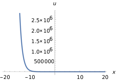
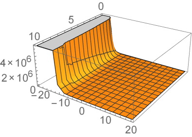
Figure 1: 2D and 3D shape of Eq.(21)

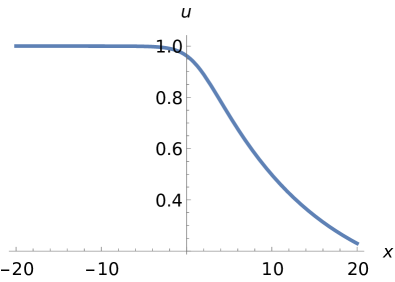
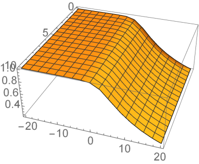
Figure 2: 2D and 3D shape of Eq.(24)

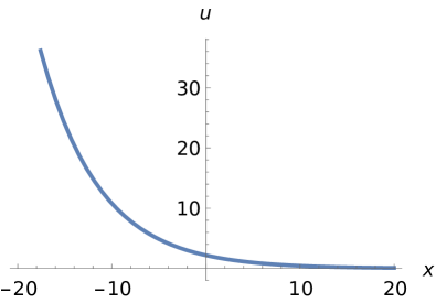
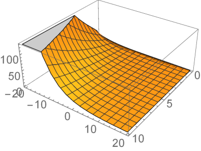
Figure 3: 2D and 3D shape of Eq.(27)

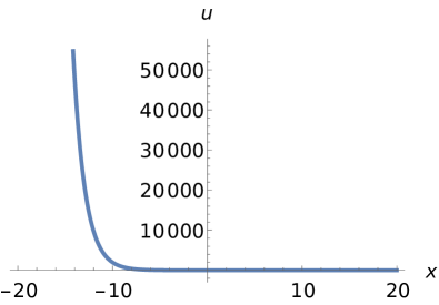
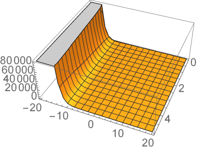
Figure 4: 2D and 3D shape of Eq.(30)

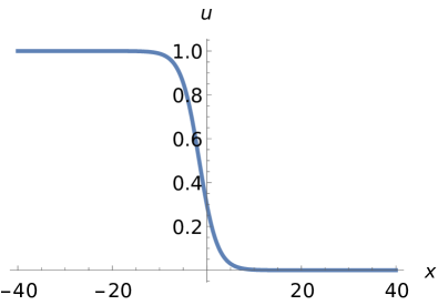
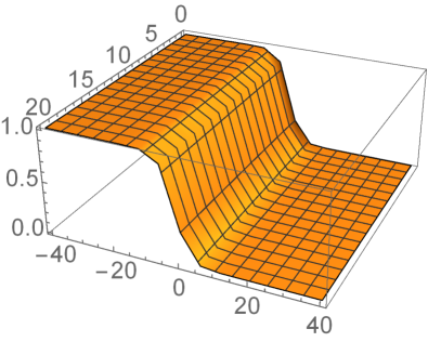
Figure 5: 2D and 3D shape of Eq.(33)

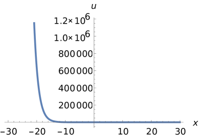
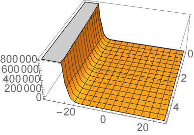
Figure 6: 2D and 3D shape of Eq.(36)

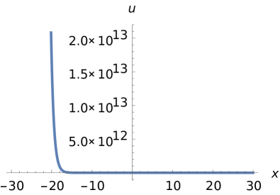
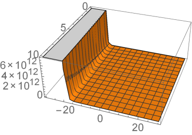
Figure 7: 2D and 3D shape of Eq.(39)

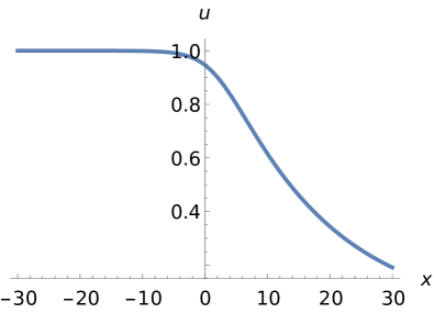
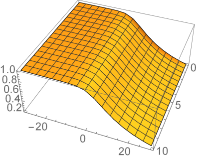
Figure 8: 2D and 3D shape of Eq.(42)

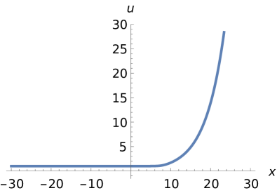
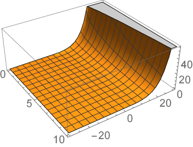
Figure 9: 2D and 3D shape of Eq.(45)

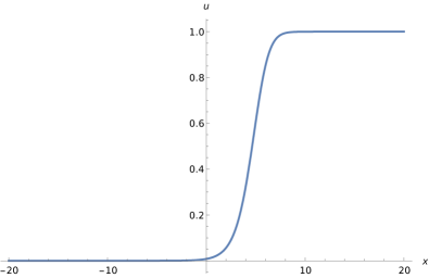
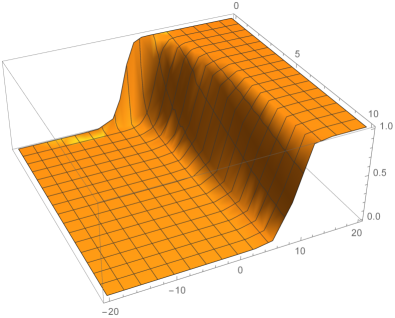
Figure 10: 2D and 3D shape of Eq.(57)

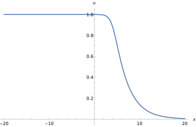
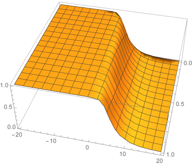
Figure 11: 2D and 3D shape of Eq.(60)

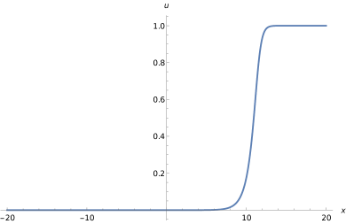
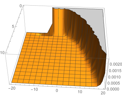
Figure 12: 2D and 3D shape of Eq.(63)

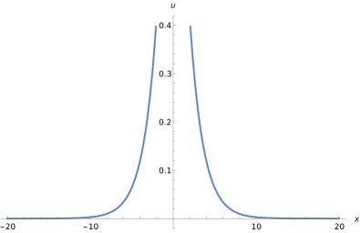
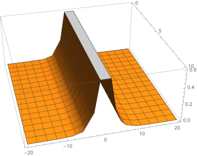
Figure 13: 2D and 3D shape of Eq.(66)

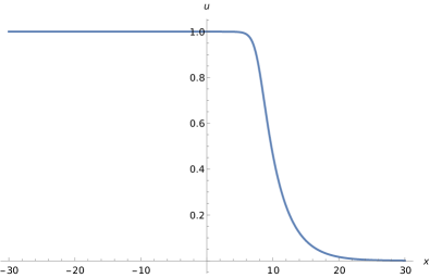
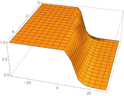
Figure 14: 2D and 3D shape of Eq.(69)

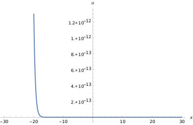
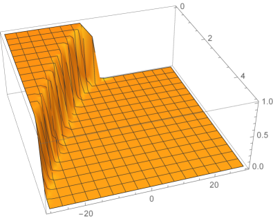
Figure 15: 2D and 3D shape of Eq.(72)

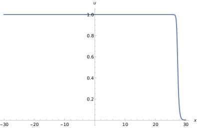
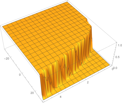
Figure 16: 2D and 3D shape of Eq.(75)

6 Conclusion

In this study, the Exp function and exponential rational function methods are used to find the exact solution for the time fractional GBF equation. This generates quite few coefficients and some have been taken into account in providing various analytical solutions. We verified all of the TF-GBF equation’s analytic solutions ousing the coefficients and the 2D and 3D plots are also included.

References

• [1] K.B. Oldham, J. Spanier, The fractional calculus, (Academic Press, Ny, 1974).
• [2] I. Podlubny, Fractional Differential Equations (Academic Press, Ny, 1999).
• [3] A. Kilbas, H. Srivatsava, J. Trujillo, Theory and Applications of Fractional Differential Equations (North Holland, NY, 2006).
• [4] G. Jumarie, Cauchy’s integral formula via modified Riemann-Liouville derivative for analytic functions of fractional order, Appl.Math.Letter., 23, (2010) 1444-1450.
• [5] M. Eslami, Exact traveling wave solutions to the fractional coupled nonlinear Schrodinger equations, Appl.Math.Comput., 285, (2016) 141-148.
• [6] Q. Huang, R. Zhdanov Symmetries and exact solutions of the time fractional Harry-Dym equation with Riemann-Liouville derivative, Phys. A., 409, (2014) 110-118.
• [7] A. Bekir, New exact travelling wave solutions of some complex nonlinear equations, Commun. Nonlinear Sci., 14(4), (2009) 1069–1077.
• [8] M. Mirzazadeh, M. E. Slami, E. Zerrad et al, Optical solitons in nonlinear directional couplers by sine-cosine function method and Bernoulli’s equation approach, Nonlinear Dynam., 81, (2015), 1933–1949.
• [9] A. Wazwaz, The tanh method: exact solutions of the sine-Gordon and the sinh-Gordon equations, Appl. Math. Comput., 167(2), (2005), 1196 - 1210.
• [10] A. M. A. El-Sayed, M. Gaber, The Adomian decomposition method for solving partial differential equations of fractal order in finite domains, Phys. Lett. A, 359(3), (2006), 175-182.
• [11] J. F. Alzaidy, Fractional Sub-Equation Method and its Applications to the Space-Time Fractional Differential Equations in Mathematical Physics, Br. J. of Maths. Comp. Sci., 2, (2013), 152-163.
• [12] S. Guo, Y. Mei, Y. Li, Y. Sun, The improved fractional sub-equation method and its applications to the space-time fractional differential equations in fluid mechanics, 76, (2012), 407-411.
• [13] C. C. Wu, A Fractional Variational Iteration Method for Solving Fractional Nonlinear Differential Equations, Comput. Math. Appl., 61(8), (2011), 2186-2190.
• [14] B. Lu, The first integral method for some time fractional differential equations, J.Math.Anal.Appl., 395(2), (2012), 684-693.
• [15] A. Bekir, O. Guner, O. Unsal, The first integral method for exact solutions of nonlinear fractional differential equations, J. Comput. Nonlinear Dyn., 10(2), (2015), 463–470.
• [16] W. Liu, K. Chen, The functional variable method for finding exact solutions of some nonlinear time-fractional differential equations, Pramana-J.Phys., (81), (2013), 377-384.
• [17] Y. Pandir, Y. Gurefe, E. Misirli, New Exact Solutions of the Time-Fractional Nonlinear Dispersive KdV Equation, Int. J. Model. Optim., 3(4), (2013), 349-352.
• [18] J. H. He, S. K. Elagan, Z. B. Li, Geometrical explanation of the fractional complex transform and derivative chain rule for fractional calculus, Phys. Lett. A., 376, (2012), 257–259.
• [19] J. H. He, X. H. Wu, Exp-function method for nonlinear wave equations, Chaos Soliton Fract, 30(3), (2006), 700-708.
• [20] M. A. Noor, S. D. Mohyud-Din,A. Waheed, Exp-function Method for Generalized Traveling Solutions of Master Partial Differential Equation, Acta Appl. Math., 104(2), (2008), 131-137.
• [21] A. Ebaid, An improvement on the Exp-function method when balancing the highest order linear and nonlinear terms, J. Math.Anal. Appl, 392(1), (2012), 1-5.
• [22] J. H. He, M. A. Abdou, New periodic solutions for nonlinear evolution equations using Exp-function method, Chaos Soliton. Fract., 34, (2007), 1421–1429.
• [23] J. He, Exp-function method for fractional differential equations, Int. J. Nonlinear Sci. Numer. Simul.,14(6), (2013), 363-366.
• [24] A. Bekir,O. GunerΒ O, Exact solutions of nonlinear fractional differential equations by ${G^{\prime}}/G)$- expansion method, Chin Phys B., 22(11), 2013, 110202.
• [25] S. Zhang, Q. A. Zong, D. Liu, Q. Gao, A generalized Exp-function method for fractional Riccati differential equations, Commun. Fract. Calculus., 1, (2010), 48-51.
• [26] B. Zheng, Exp-Function Method for Solving Fractional Partial Differential Equations, Sci. World. J., 2013, (2013), Article ID 465723, 8 pages.
• [27] L. M. Yan, F. S. Xu, Generalized Exp function method for nonlinear space-time fractional differential equations, Thermal Sci., 18(5), (2015), 1573-1576.
• [28] H. Demiray, A travelling wave solution to the KdV–Burgers equation, Appl. Math. Comput., 154, (2004), 665-670.
• [29] E. Aksoy, M. Kaplan, A. Bekir, Exponential rational function method for space–time fractional differential equations, Waves Random Complex., 26, (2016), 142-151.
• [30] A. Bekir, M. Kaplan, Exponential rational function method for solving nonlinear equations arising in various physical models, Chin. J. Phys., 54(3), (2016), 365-370.
• [31] S. T. Mohyud-Din,S. Bibi. Exact solutions for nonlinear fractional differential equations using exponential rational function method, Opt. Quantum Electron., 49(64), (2017).
• [32] G. Jumarie, Modified Riemann-Liouville derivative and fractional Taylor series of non differentiable functions further results, Comput. Math. Appl., 51, (200), 1367-1376.
• [33] G. Jumarie, Table of some basic fractional calculus formulae derived from a modified Riemann–Liouville derivative for non-differentiable functions, Appl. Maths. Lett., 22(3), (2009), 378-385.
• [34] J. H. He, Z. B. Li, Converting fractional differential equations into partial differential equations, Therm Sci., 16(2), (2012), 331-334.
• [35] Z. B. Li, J. H. He, Fractional Complex Transform for Fractional Differential Equations, Math. Comput. Appl.,15(5), (2010), 970-973.