Stable and accurate numerical methods for generalized Kirchhoff-Love plates

Abstract

Efficient and accurate numerical algorithms are developed to solve a generalized Kirchhoff-Love plate model subject to three common physical boundary conditions: (i) clamped; (ii) simply supported; and (iii) free. We solve the model equation by discretizing the spatial derivatives using second-order finite-difference schemes, and then advancing the semi-discrete problem in time with either an explicit predictor-corrector or an implicit Newmark-Beta time-stepping algorithm. Stability analysis is conducted for the schemes and the results are used to determine stable time steps in practice. A series of carefully chosen test problems are solved to demonstrate the properties and applications of our numerical approaches. The numerical results confirm the stability and 2nd-order accuracy of the algorithms, and are also comparable with experiments for similar thin plates. As an application, we illustrate a strategy to identify the natural frequencies of a plate using our numerical methods in conjunction with a fast Fourier transformation (FFT) power spectrum analysis of the computed data. Then we take advantage of one of the computed natural frequencies to simulate the interesting physical phenomena known as resonance and beat for a generalized Kirchhoff-Love plate.

65M06 , 65M12, 74S20

1 Introduction

Thin-walled elastic solids, often referred to as plates or shells, are ubiquitous in engineerings and applied sciences. Examples of plates or shells can be found in many common mechanical and biological structures such as dome-shaped stadium rooftops, airplane fuselages, vessel walls and aortic valves, etc. Adequately understanding the intrinsic properties of plates (shells) is crucial for the various applications involving these structures. Therefore, the investigation of mathematically modeling plate-like structures and the subsequent development of numerical approximations for their solutions have long been active areas of research. Noting that the difference between a plate and a shell lies in its precast stress-free shape, which is flat for a plate and curved for a shell.

To study plate structures analytically, numerous theories have been developed over the years aiming at predicting the various key physical characteristics; see [1, 2, 3, 4, 5] and the references therein. The classical Kirchhoff-Love plate theory, which was developed way back in 1888 under the assumptions that the thickness of the plate remains fixed and any straight lines normal to the reference surface remain straight and normal to the reference surface after deformation, captures the bending dynamics of a plate in response to a transverse load and determines the propagation of waves in the plate [4]. As an extension to the Kirchhoff-Love model, the Mindlin-Reissner plate theory takes a first-order shear deformation into account and no longer assumes that straight lines normal to the reference surface remain normal during a deformation [6]. As is reviewed in [5], there are also many other plate theories that are able to describe more sophisticated nonlinear physical phenomena, which make them viable choices for modeling complicated engineering applications. For example, the Koiter shell theory [7] and its recent variant that incorporates viscoelasticity [8] are often used in biomedical engineering to model artery walls.

These plate theories are in general derived by utilizing the disparity in the length scales of the thin structures, and significantly reduce the complexity of the three-dimensional (3D) continuum mechanics problem to a two-dimensional one (2D). The governing equations of a plate theory typically deal with variables defined only on a reference surface that resides on a 2D domain; for an isotropic and homogeneous plate, its middle (or center) surface is used as reference. See Figure 1 for a schematic illustration of a 3D thin plate and its 2D reference surface. Physical assumptions of the underlining plate theories also provide means of calculating the load-carrying and deflection characteristics of the original thin-walled structures; and therefore, the complete deformation and stress fields of a 3D thin structure can be inferred from the solution of its reference surface. It is generally expected that the thinner the structure, the more accurate the plate theory.

Figure 1: Cartoon illustration of a deformed thin plate and its reference surface.

From both the analytical and numerical points of view, 2D plate theories are immensely more tractable than 3D solid mechanical models. The plate theories are especially appealing to researchers exploring multi-physical problems, such as fluid-structure interaction (FSI) problems involving thin-walled elastic structures [9, 10, 8], whereby multiple physical subproblems are dealt with simultaneously. Although greatly simplified from the full 3D continuum mechanics problem, governing equations for plates are still too complicated to be solved analytically, except for a limited number of cases with simple specifications [11]. Efficient and accurate numerical approximations for the solutions are therefore of greater interest in practice. However, due to numerical challenges posed by the high-order spatial derivatives that are associated with the bending effect of plates, the development of stable and accurate numerical methods for solving plate equations is non-trivial. Many numerical approaches have been developed for solving various plate models based on common discretization methods such as finite difference [12, 13], finite element (FEM) [14, 15, 16, 17, 18, 19, 20, 21, 22], and boundary element (BEM) [23], to name just a few. More recently, new computational methods developed from the isogeometric analysis have also emerged; see [24] for an example of solving the Reissner-Mindlin shell using the isogeometric analysis.

In this paper, we present accurate and efficient numerical approximations of a generalized Kirchhoff-Love model that incorporates additional important physics, such as linear restoration, tension and visco-elasticity, for isotropic and homogeneous thin plates. The generalized model equation is spatially discretized with a standard second-order accurate finite difference method and integrated in time using either an explicit predictor-corrector or an implicit time-stepping scheme. Stability analysis is performed and the results are utilized to determine stable time steps for the proposed numerical schemes. Stable and accurate numerical boundary conditions are also investigated for the most common physical boundary conditions (i.e., clamped, simply supported and free). Carefully designed test problems are solved using all the proposed schemes for numerical validations. Interesting applications using the numerical methods are also discussed.

The remainder of the paper is organized as follows. In Section 2, we present the governing equation and its boundary conditions for a generalized Kirchhoff-Love model. The numerical algorithms for solving the model equation are discussed in Section 3. We analyze the stability of the numerical schemes and lay out a strategy for determining stable time steps for the algorithms in Section 4. Numerical results that provide verification of the stability and accuracy of the schemes, as well as cross-validation with experiments, are presented in Section 5. Finally, concluding remarks are made in Section 6.

2 Governing equations

The classical Kirchhoff-Love plate model concerns the small deflection of thin plates that is used as a simplified theory of solid mechanics to determine the stresses and deformations in the plates subject to external forcings. The governing equation for an isotropic and homogeneous plate is a single time-dependent biharmonic partial differential equation (PDE) for the transverse displacement of the plate’s middle surface. It is derived by balancing the external loads with the internal bending force that tends to restore the plate to its stress-free state. In this paper, we consider a plate model that is generalized from the classical Kirchhoff-Love equation by including additional terms to account for more physical effects, such as linear restoration, tension and visco-elasticity.

To be specific, this work concerns developing numerical algorithms for solving the following generalized Kirchhoff-Love model for an isotropic and homogeneous plate with constant thickness $h$,

(1) $${\rho}{h}\frac{\partial^{2}w}{\partial t^{2}}=-{K}_{0}w+{T}\nabla^{2}w-{D}\nabla^{4}w-{K}_{1}\frac{\partial w}{\partial t}+{T}_{1}\nabla^{2}\frac{\partial w}{\partial t}+F(\mathbf{x},t),$$

where $w(\mathbf{x},t)$ with $\mathbf{x}\in\Omega\subset\mathbb{R}^{2}$ is the transverse displacement of the middle surface subject to some given body force $F$. Here, ${\rho}$ denotes density, ${K}_{0}$ is the linear stiffness coefficient that acts as a linear restoring force, ${T}$ is the tension coefficient, and ${D}={E}{h}^{3}/(12(1-\nu))$ represents the flexural rigidity with $\nu$ and $E$ being the Poisson’s ratio and Young’s modulus, respectively. The term with coefficient ${K}_{1}$ is a linear damping term, while the term with coefficient ${T}_{1}$ is a visco-elastic damping term that tends to smooth high-frequency oscillations in space. Noting that the visco-elastic damping is often added to model vascular structures in haemodynamics [8].

On the boundary, one of the following physical boundary conditions is imposed; namely, for $\mathbf{x}\in\partial\Omega$, we have

(2) clamped: $$w=0, \frac{\partial w}{\partial\mathbf{n}}=0;$$

(3) supported: $$w=0, \frac{\partial^{2}w}{\partial\mathbf{n}^{2}}+\nu\frac{\partial^{2}w}{\partial\mathbf{t}^{2}}=0;$$

(4) free: $$\frac{\partial^{2}w}{\partial\mathbf{n}^{2}}+\nu\frac{\partial^{2}w}{\partial\mathbf{t}^{2}}=0, \frac{\partial}{\partial\mathbf{n}}\left[\frac{\partial^{2}w}{\partial\mathbf{n}^{2}}+\left(\nu-2\right)\frac{\partial^{2}w}{\partial\mathbf{t}^{2}}\right]=0,$$

where $\partial/\partial{\mathbf{n}}$ and $\partial/\partial{\mathbf{t}}$ are the normal and tangential derivatives defined on the boundary of the domain. It is important to point out that, for a rectangular plate, the free boundary conditions (4) must be complemented by a corner condition that imposes zero forcing [12]; in other words, we also impose $\partial^{2}w/\partial x\partial y=0$ at the corners of a rectangular plate. Note that for notational brevity the functional dependence on $(\mathbf{x},t)$ has been suppressed in the statement of the boundary conditions.

Appropriate initial conditions need to be specified to complete the statement of the governing equations. Specifically, we assign

(5) $$w(\mathbf{x},0)=w_{0}(\mathbf{x})\leavevmode\nobreak\ \text{and}\leavevmode\nobreak\ \frac{\partial w}{\partial t}(\mathbf{x},0)=v_{0}(\mathbf{x})$$

as the initial conditions with $w_{0}(\mathbf{x})$ and $v_{0}(\mathbf{x})$ representing two given functions that prescribe the plate’s initial displacement and velocity.

3 Numerical methods

In this section, we present the numerical approaches to solve the governing equation (1) subject to the boundary conditions (2)–(4). Standard centered finite difference methods of second-order accuracy are used for the discretization of all the spatial derivatives, and then the resulted semi-discrete equations are integrated in time using an appropriate time-stepping scheme.

Let $\Omega_{h}$ denote a mesh covering the domain $\Omega$, and let $\mathbf{x}_{\mathbf{i}}\in\Omega_{h}$ denote the coordinates of a grid point with multi-index $\mathbf{i}=(i_{1},i_{2})$. The time-dependent grid function that approximates the displacement on the mesh is given by $w_{\mathbf{i}}(t)\approx w(\mathbf{x}_{\mathbf{i}},t)$. Similarly, $F_{\mathbf{i}}$ is used to denote the given forcing function evaluated at $\mathbf{x}_{\mathbf{i}}$; namely, $F_{\mathbf{i}}(t)=F(\mathbf{x}_{\mathbf{i}},t)$. We spatially discretize the governing equation and its boundary conditions by replacing the differential operators with the corresponding finite-difference operators (distinguished with a subscript $h$) to derive the semi-discrete equations,

(6) $${\rho}{h}\frac{d^{2}w_{\mathbf{i}}}{dt^{2}}=-{K}_{0}w_{\mathbf{i}}+{T}\nabla_{h}^{2}w_{\mathbf{i}}-{D}\nabla_{h}^{4}w_{\mathbf{i}}-{K}_{1}\frac{dw_{\mathbf{i}}}{dt}+{T}_{1}\nabla_{h}^{2}\frac{dw_{\mathbf{i}}}{dt}+F_{\mathbf{i}},\leavevmode\nobreak\ \forall\mathbf{x}_{\mathbf{i}}\in\Omega_{h},$$

as well as the following discrete boundary conditions. For $\forall\mathbf{x}_{\mathbf{i}_{b}}\in\partial\Omega_{h}$, the numerical boundary conditions are given by

(7) clamped: $$w_{\mathbf{i}_{b}}=0, \frac{\partial_{h}w_{\mathbf{i}_{b}}}{\partial_{h}\mathbf{n}}=0;$$

(8) supported: $$w_{\mathbf{i}_{b}}=0, \frac{\partial_{h}^{2}w_{\mathbf{i}_{b}}}{\partial_{h}\mathbf{n}^{2}}+\nu\frac{\partial_{h}^{2}w_{\mathbf{i}_{b}}}{\partial_{h}\mathbf{t}^{2}}=0;$$

(9) free: $$\frac{\partial_{h}^{2}w_{\mathbf{i}_{b}}}{\partial_{h}\mathbf{n}^{2}}+\nu\frac{\partial_{h}^{2}w_{\mathbf{i}_{b}}}{\partial_{h}\mathbf{t}^{2}}=0, \frac{\partial_{h}}{\partial_{h}\mathbf{n}}\left[\frac{\partial_{h}^{2}w_{\mathbf{i}_{b}}}{\partial_{h}\mathbf{n}^{2}}+\left(\nu-2\right)\frac{\partial_{h}^{2}w_{\mathbf{i}_{b}}}{\partial_{h}\mathbf{t}^{2}}\right]=0.$$

For numerical purposes, we rewrite (6) into a system of first-order ODEs. If we denote $v_{\mathbf{i}}$ and $a_{\mathbf{i}}$ the numerical approximations of the velocity and acceleration at grid point $\mathbf{x}_{\mathbf{i}}$, equation (6) can thus be conveniently written as

(10) $$\frac{dw_{\mathbf{i}}}{dt}(t)=v_{\mathbf{i}}(t),$$

(11) $$\frac{dv_{\mathbf{i}}}{dt}(t)=a_{\mathbf{i}}(t),$$

(12) $${\rho}{h}a_{\mathbf{i}}(t)=-{{\mathcal{K}}_{h}}w_{\mathbf{i}}(t)-{{\mathcal{B}}_{h}}v_{\mathbf{i}}(t)+F_{\mathbf{i}}(t),$$

where the operators for the internal forces ${\mathcal{K}}_{h}$ and the damping forces ${\mathcal{B}}_{h}$ are introduced below to simplify the notations;

(13) $${\mathcal{K}}_{h}={K}_{0}-{T}\nabla_{h}^{2}+{D}\nabla_{h}^{4}\quad\text{and}\quad{\mathcal{B}}_{h}={K}_{1}-{T}_{1}\nabla_{h}^{2}.$$

In this paper, two time-stepping methods are considered to advance the ODE system in time. In particular, one of the methods is an explicit predictor-corrector scheme that consists of a second-order Adams-Bashforth (AB2) predictor and a second-order Adams-Moulton (AM2) corrector, while the other one is an implicit Newmark-Beta scheme of second-order accuracy [25]. We refer to the former scheme as PC22 scheme and the latter one as NB2 scheme for short.

To simplify the discussion, the algorithms are developed for a fixed time-step $\Delta t$ so that $t_{n}=n\Delta t$. Let the numerical solutions of (10)–(12) at time $t_{n}$ be $w_{\mathbf{i}}^{n}\approx w_{\mathbf{i}}(t_{n})$, $v_{\mathbf{i}}^{n}\approx v_{\mathbf{i}}(t_{n})$, and $a_{\mathbf{i}}^{n}\approx a_{\mathbf{i}}(t_{n})$, and denote $F_{\mathbf{i}}^{n}=F(\mathbf{x}_{\mathbf{i}},t_{n})$. The goal of a time-stepping algorithm is to determine the solutions at a new time given solutions at previous time levels.

First, we describe the PC22 scheme in Algorithm 1.

Input: solutions at two previous time levels; i.e., $(w_{\mathbf{i}}^{n},v_{\mathbf{i}}^{n},a_{\mathbf{i}}^{n})$ and $(w_{\mathbf{i}}^{n-1},v_{\mathbf{i}}^{n-1},a_{\mathbf{i}}^{n-1})$
Output: solutions at the new time level; i.e., $(w_{\mathbf{i}}^{n+1},v_{\mathbf{i}}^{n+1},a_{\mathbf{i}}^{n+1})$
Procedures:
Stage I: predict solutions using a second-order Adams-Bashforth (AB2) predictor

$$\forall\mathbf{x}_{\mathbf{i}}\in\Omega_{h}:\quad\begin{cases}w_{\mathbf{i}}^{p}=w_{\mathbf{i}}^{n}+\Delta t\left(\frac{3}{2}v_{\mathbf{i}}^{n}-\frac{1}{2}v_{\mathbf{i}}^{n-1}\right)\\ v_{\mathbf{i}}^{p}=v_{\mathbf{i}}^{n}+\Delta t\left(\frac{3}{2}a_{\mathbf{i}}^{n}-\frac{1}{2}a_{\mathbf{i}}^{n-1}\right)\\ a^{p}_{\mathbf{i}}=\frac{1}{{\rho}{h}}\left(-{{\mathcal{K}}_{h}}w^{p}_{\mathbf{i}}-{{\mathcal{B}}_{h}}v^{p}_{\mathbf{i}}+F^{n+1}_{\mathbf{i}}\right)\end{cases}$$

Stage II: correct solutions using a second-order Adams-Molton (AM2) corrector

$$\forall\mathbf{x}_{\mathbf{i}}\in\Omega_{h}:\quad\begin{cases}w_{\mathbf{i}}^{n+1}=w_{\mathbf{i}}^{n}+\Delta t\left(\frac{1}{2}v_{\mathbf{i}}^{n}+\frac{1}{2}v_{\mathbf{i}}^{p}\right)\\ v_{\mathbf{i}}^{n+1}=v_{\mathbf{i}}^{n}+\Delta t\left(\frac{1}{2}a_{\mathbf{i}}^{n}+\frac{1}{2}a_{\mathbf{i}}^{p}\right)\\ a^{n+1}_{\mathbf{i}}=\frac{1}{{\rho}{h}}\left(-{{\mathcal{K}}_{h}}w^{n+1}_{\mathbf{i}}-{{\mathcal{B}}_{h}}v^{n+1}_{\mathbf{i}}+F^{n+1}_{\mathbf{i}}\right)\end{cases}$$

Remark:Boundary conditions are applied after both the predictor and corrector stages to fill in the solutions at ghost and/or boundary grid points. Note that numerical boundary conditions for $v$ and $a$ are derived from those for $w$ by taking the appropriate time derivatives of (7)–(9).

Algorithm 1 PC22 time-stepping scheme

Second, we consider the Newmark-Beta scheme for solving our problem (10)–(12). The so-called Newmark-Beta scheme is a general procedure proposed by Newmark for the solution of problems in structural dynamics [25]. Given acceleration, the scheme updates the velocity and displacement by solving

(14) $$\begin{cases}w_{\mathbf{i}}^{n+1}=w_{\mathbf{i}}^{n}+\Delta tv_{\mathbf{i}}^{n}+\frac{\Delta t^{2}}{2}\left[(1-2\beta)a_{\mathbf{i}}^{n}+2\beta a_{\mathbf{i}}^{n+1}\right],\\ v_{\mathbf{i}}^{n+1}=v_{\mathbf{i}}^{n}+\Delta t\left[(1-\gamma)a_{\mathbf{i}}^{n}+\gamma a_{\mathbf{i}}^{n+1}\right],\end{cases}$$

where the acceleration in our case is given by

(15) $${\rho}{h}a^{n+1}_{\mathbf{i}}=-{{\mathcal{K}}_{h}}w_{\mathbf{i}}^{n+1}-{{\mathcal{B}}_{h}}v_{\mathbf{i}}^{n+1}+F_{\mathbf{i}}^{n+1}.$$

We note that the scheme is unconditionally stable if $1/2\leq\gamma\leq 2\beta$, whereas it is conditionally stable if $\gamma>\max\{1/2,2\beta\}$.

Instead of solving the above implicit system for $w_{\mathbf{i}}^{n+1}$, $v_{\mathbf{i}}^{n+1}$ and $a_{\mathbf{i}}^{n+1}$ all at the same time, we use (14) to eliminate $w_{\mathbf{i}}^{n+1}$ and $v_{\mathbf{i}}^{n+1}$ in (15), and then solve a smaller system for $a_{\mathbf{i}}^{n+1}$ only. The complete algorithm for this scheme is summarized in Algorithm 2.

Input: solutions at the previous time level; i.e., $(w_{\mathbf{i}}^{n},v_{\mathbf{i}}^{n},a_{\mathbf{i}}^{n})$
Output: solutions at the new time level; i.e., $(w_{\mathbf{i}}^{n+1},v_{\mathbf{i}}^{n+1},a_{\mathbf{i}}^{n+1})$
Procedures:
Stage I. compute a first-order prediction for displacement and velocity

$$\forall\mathbf{x}_{\mathbf{i}}\in\Omega_{h}:\quad\begin{cases}w_{\mathbf{i}}^{p}=w_{\mathbf{i}}^{n}+\Delta tv_{\mathbf{i}}^{n}+\frac{\Delta t^{2}}{2}(1-2\beta)a_{\mathbf{i}}^{n}\\ v_{\mathbf{i}}^{p}=v_{\mathbf{i}}^{n}+\Delta t(1-\gamma)a_{\mathbf{i}}^{n}\end{cases}$$

Stage II. solve a system of equations for acceleration at $t_{n+1}$

$$\forall\mathbf{x}_{\mathbf{i}}\in\Omega_{h}:\quad\left({\rho}{h}+\beta\Delta t^{2}{\mathcal{K}}_{h}+\gamma\Delta t{\mathcal{B}}\right)a^{n+1}_{\mathbf{i}}=-{{\mathcal{K}}_{h}}w_{\mathbf{i}}^{p}-{{\mathcal{B}}_{h}}v_{\mathbf{i}}^{p}+F_{\mathbf{i}}^{n+1}$$

Stage III. solve for displacement and velocity at $t_{n+1}$

compute $$w_{\mathbf{i}}^{n+1} v_{\mathbf{i}}^{n+1}$$ and explicitly from (14)

Remark: In this paper, we set $\beta=1/4$ and $\gamma=1/2$. With this choice of parameters, the scheme is second-order accurate and unconditionally stable. We also note that boundary conditions are applied after stages I and III to fill in the solutions of $w$ and $v$ at ghost and/or boundary grid points. For stage II, equations for acceleration at ghost and boundary nodes are replaced with boundary conditions.

Algorithm 2 NB2 time-stepping scheme

4 Stability analysis and time step determination

We study the stability of the schemes and use the analytical results to determine stable time steps in practical computations. As is already pointed out in [25] that the implicit NB2 time-stepping scheme is unconditionally stable, the focus of the stability analysis here is on the explicit PC22 scheme.

4.1 Stability of the PC22 scheme

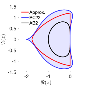
Figure 2: Regions of absolute stability for the PC22 time-step scheme and the scheme with an AB2 predictor only. The approximated region of stability using a half super-ellipse is also depicted in the plot. Here, $z=\lambda\Delta t$ with $\lambda$ being the time-stepping eigenvalue and $\Delta t$ representing the time step. $\Re(z)$ and $\Im(z)$ represent the real and imaginary parts of the complex number $z$.

Applying the PC22 scheme to the Dahlquist test equation $\eta^{\prime}=\lambda\eta$ leads to the characteristic polynomial for a complex-valued amplification factor $\zeta$. Letting $z=\lambda\Delta t$, the roots of the characteristic equation are found to be

(16) $$\zeta(z)=\dfrac{1}{2}\left(1+z+\frac{3}{4}z^{2}\pm\sqrt{\left(1+z+\frac{3}{4}z^{2}\right)^{2}-z^{2}}\right).$$

The region of absolute stability for the PC22 time-stepping scheme is the set of complex values $z$ for which the roots of the characteristic polynomial satisfy $|\zeta(z)|\leq 1$.

The stability region can be used to find the time step restriction for a typical problem. However, it is not straightforward to obtain a stable time step by solving the inequality $|\zeta(z)|\leq 1$ directly from (16), so a half super-ellipse is introduced as an approximation of the stability region. To be specific, we define the half super-ellipse by

(17) $$\left|\frac{\Re(z)}{a}\right|^{n}+\left|\dfrac{\Im(z)}{b}\right|^{n}\leq 1\quad\text{and}\quad\Re(z)\leq 0,$$

where $\Re(z)$ and $\Im(z)$ denote the real and imaginary parts of $z$, respectively. We want the half super-ellipse to be completely enclosed by the actual region of stability and to be as large as possible. Given a time-stepping eigenvalue $\lambda$, it is much easier to find a sufficient condition for stability by requiring $\lambda\Delta t$ to be inside the approximated region defined by (17). It is found that the above half super-ellipse makes a good approximation for the stability region of the PC22 time-stepping scheme by setting $a=1.75,b=1.2$ and $n=1.5$.

The region of absolute stability for the PC22 time-stepping scheme, together with the approximated region, is shown in Figure 2. For comparison purposes, we also plot the stability region for the scheme that only uses an AB2 predictor in the same figure. We can see that by including a corrector step the PC22 scheme has a much larger stability region than the predictor alone, and the stability region includes the imaginary axis so that the scheme can be used for problems with no dissipations. From the plot, we can also see that the half super-ellipse that is chosen to be an approximation fits perfectly inside the original stability region for the PC22 scheme.

4.2 Time-step determination

A strategy for the determination of stable time steps to be used in Algorithms 1 & 2 is outlined here. We first transform the semi-discrete problem (10)–(12) into Fourier Space, and then derive a stable time step by imposing the condition that the product of the time step and any eigenvalue of the Fourier transformation of the difference operators lies inside the stability region of a particular time-stepping method for all wave numbers.

For simplicity of presentation, we assume the plate resides on a unit square domain ($\Omega=[0,1]\times[0,1]$), and the solution is 1-periodic in both $x$ and $y$ directions. Results on a more general domain can be readily obtained by mapping the general domain to a unit square. After Fourier transforming the homogeneous version of equations (10)–(12) (i.e., assuming $F_{\mathbf{i}}(t)\equiv 0$), an ODE system for the transformed variables ($\hat{w}$, $\hat{v}$) is derived with $\omega=(\omega_{x},\omega_{y})$ denoting any wavenumber pair,

(18) $$\begin{bmatrix}\hat{w}(\omega,t)\\ \hat{v}(\omega,t)\end{bmatrix}_{t}={\hat{Q}(\omega)}\begin{bmatrix}\hat{w}(\omega,t)\\ \hat{v}(\omega,t)\end{bmatrix},\leavevmode\nobreak\ \leavevmode\nobreak\ \text{where}\leavevmode\nobreak\ \leavevmode\nobreak\ \hat{Q}(\omega)=\begin{bmatrix}0&1\\ -\hat{{\mathcal{K}}}(\omega)&-\hat{{\mathcal{B}}}(\omega)\end{bmatrix}.$$

Here $\hat{{\mathcal{K}}}$ and $\hat{{\mathcal{B}}}$ are the Fourier transformations of the difference operators ${\mathcal{K}}_{h}/(\rho h)$ and ${\mathcal{B}}_{h}/(\rho h)$, respectively. Let $k_{\omega_{x}}={2\sin({\omega_{x}h_{x}}/{2})}/{h_{x}}$ and $k_{\omega_{y}}={2\sin({\omega_{y}h_{y}}/{2}})/{h_{y}}$, where $h_{x}$ and $h_{y}$ are the grid spacings in the corresponding directions; then we have

$$\hat{{\mathcal{K}}}(\omega) =\frac{1}{\rho{h}}\left[K_{0}+T\left(k^{2}_{\omega_{x}}+k^{2}_{\omega_{y}}\right)+D\left(k^{4}_{\omega_{x}}+2k^{2}_{\omega_{x}}k^{2}_{\omega_{y}}+k^{4}_{\omega_{y}}\right)\right],$$

$$\hat{{\mathcal{B}}}(\omega) =\frac{1}{\rho{h}}\left[K_{1}+T_{1}\left(k^{2}_{\omega_{x}}+k^{2}_{\omega_{y}}\right)\right].$$

Noting that both $\hat{{\mathcal{K}}}$ and $\hat{{\mathcal{B}}}$ are non-negative for any $\omega$. In the analysis to follow, their maximum values denoted by $\hat{{\mathcal{K}}}_{M}$ and $\hat{{\mathcal{B}}}_{M}$ are of interest, which are attained when $\omega_{x}h_{x}=n\pi$ and $\omega_{y}h_{y}=m\pi$ ($n,m\in\mathbb{Z}$); namely,

(19) $$\hat{{\mathcal{K}}}_{M} =\frac{1}{\rho{h}}\left[K_{0}+4{T}\left(\frac{1}{h_{x}^{2}}+\frac{1}{h_{y}^{2}}\right)+16D\left(\frac{1}{h_{x}^{2}}+\frac{1}{h_{y}^{2}}\right)^{2}\right],$$

(20) $$\hat{{\mathcal{B}}}_{M} =\frac{1}{\rho{h}}\left[K_{1}+4T_{1}\left(\frac{1}{h_{x}^{2}}+\frac{1}{h_{y}^{2}}\right)\right].$$

A numerical method is stable provided all the eigenvalues of $\hat{Q}(w)\Delta t$ lie within the stability region of the time-stepping method. The eigenvalues of the coefficient matrix $\hat{Q}(w)$ for the problem (18) are

(21) $$\hat{\lambda}(\omega)=-\frac{\hat{{\mathcal{B}}}(\omega)}{2}\pm\sqrt{\left(\frac{\hat{{\mathcal{B}}}(\omega)}{2}\right)^{2}-\hat{{\mathcal{K}}}(\omega)}.$$

For stability analysis, it suffices to consider the eigenvalue with the largest possible magnitude denoted by $\hat{\lambda}_{M}$. To find $\hat{\lambda}_{M}$, we consider the following situations.

Under-damped case. If $\left({\hat{{\mathcal{B}}}(\omega)}/{2}\right)^{2}-\hat{{\mathcal{K}}}(\omega)<0$, we obtain complex eigenvalues,

$$\hat{\lambda}(\omega)=-\frac{\hat{{\mathcal{B}}}(\omega)}{2}\pm i\sqrt{\hat{{\mathcal{K}}}(\omega)-\left(\frac{\hat{{\mathcal{B}}}(\omega)}{2}\right)^{2}}.$$

In this case, we may define

(22) $$\hat{\lambda}_{M}=-\frac{\hat{{\mathcal{B}}}_{M}}{2}\pm i\sqrt{\hat{{\mathcal{K}}}_{M}-\left(\frac{\hat{{\mathcal{B}}}_{M}}{2}\right)^{2}},$$

since $|\hat{\lambda}(\omega)|=\sqrt{\hat{{\mathcal{K}}}(\omega)}\leq\sqrt{\hat{{\mathcal{K}}}_{M}}=|\hat{\lambda}_{M}|$. Here $\hat{{\mathcal{K}}}_{M}$ and $\hat{{\mathcal{B}}}_{M}$ are the maximum values of $\hat{{\mathcal{K}}}(\omega)$ and $\hat{{\mathcal{B}}}(\omega)$ that are given by (19) and (20).

Over-damped case. If $\left({\hat{{\mathcal{B}}}(\omega)}/{2}\right)^{2}-\hat{{\mathcal{K}}}(\omega)>0$, the eigenvalues are real and are of the same form as (21). In this case, we may define

(23) $$\hat{\lambda}_{M}=-\hat{{\mathcal{B}}}_{M}.$$

This is because

$$|\hat{\lambda}(\omega)|\leq\frac{\hat{{\mathcal{B}}}(\omega)}{2}+\sqrt{\left(\frac{\hat{{\mathcal{B}}}(\omega)}{2}\right)^{2}-\hat{{\mathcal{K}}}(\omega)}\leq\hat{{\mathcal{B}}}(\omega)\leq\hat{{\mathcal{B}}}_{M}=|\hat{\lambda}_{M}|.$$

We note that $\hat{\lambda}_{M}$ introduced in (22) and (23) represent the eigenvalues of the worst-case scenario for the under-damped and over-damped cases, respectively. A sufficient condition that ensures stability for the PC22 scheme is found by letting $z=\hat{\lambda}_{M}\Delta t$ lie in the approximated stability region that is defined by the half super-ellipse in (17). Since the approximated stability region is a subset of the actual one, a time step that is sufficient to guarantee the stability of Algorithm 1 can be chosen as following,

(24) $$\Delta t={C_{\text{sf}}}{\left(\left|\frac{\Re(\hat{\lambda}_{M})}{a}\right|^{n}+\left|\frac{\Im(\hat{\lambda}_{M})}{b}\right|^{n}\right)^{-1/n}},$$

where $C_{\text{sf}}\in(0,1]$ is a stability factor (sf) that multiplies an estimate of the largest stable time step based on the above analysis. Unless otherwise noted, we choose $C_{\text{sf}}=0.9$ for the PC22 scheme throughout this paper.

In terms of the NB2 scheme, we know that it is implicit in time and stable for any time step. However, for accuracy reasons, we choose its time step based on the condition for the explicit PC22 time-stepping scheme (24), but with a much larger stability factor. Typically, we choose $C_{\text{sf}}=90$ for Algorithm 2.

5 Numerical results

We now present the results for a series of test problems to demonstrate the properties and applications of our numerical approaches. Mesh refinement studies using problems with known exact solutions are first considered to verify the stability and accuracy of the schemes. Free and forced vibrations of thin plates with various geometrical and physical configurations are then solved to further demonstrate the numerical properties of our schemes and to compare with existing results. In particular, the simulation of one test problem is cross-validated with reported experimental results. As an application, we illustrate a strategy using our numerical methods, together with fast Fourier transformation (FFT), to identify the natural frequencies of a plate, and then numerically investigate the interesting physical phenomena known as resonance and beat.

5.1 Method of manufactured solutions

As a first test, we verify the accuracy and stability of the algorithms using the method of manufactured solutions by adding forcing functions to the PDE (1) and the boundary conditions (2)–(4) so that a chosen function becomes an exact solution. The exact solution is chosen to be

(25) $$w_{e}(x,y,t)=\sin^{4}\left(\pi(x+1)\right)\sin^{4}\left(\pi(y+1)\right)\cos(2\pi t).\\$$

In order to validate the algorithms on both Cartesian and curvilinear grids, we consider a square plate ($\Omega_{S}=[-1,1]\times[-1,1]$) and an annular plate ($\Omega_{A}=\{\mathbf{x}:0.5\leq|\mathbf{x}|\leq 1\}$). Physical parameters of the governing equation are specified as $\rho h=1,K_{0}=2,T=1,D=0.01,K_{1}=5,T_{1}=0.1$ and $\nu=0.1$ for this test.

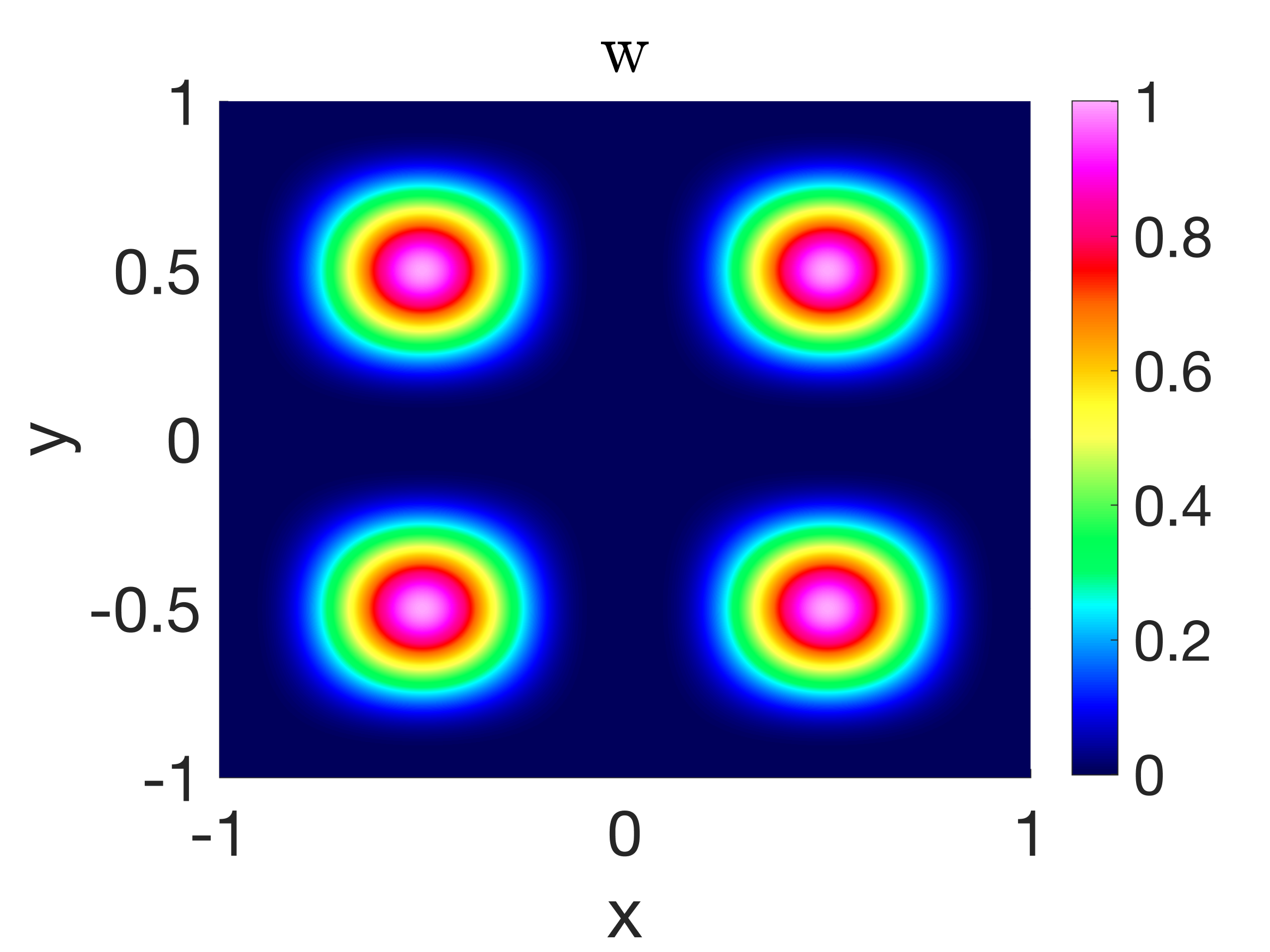
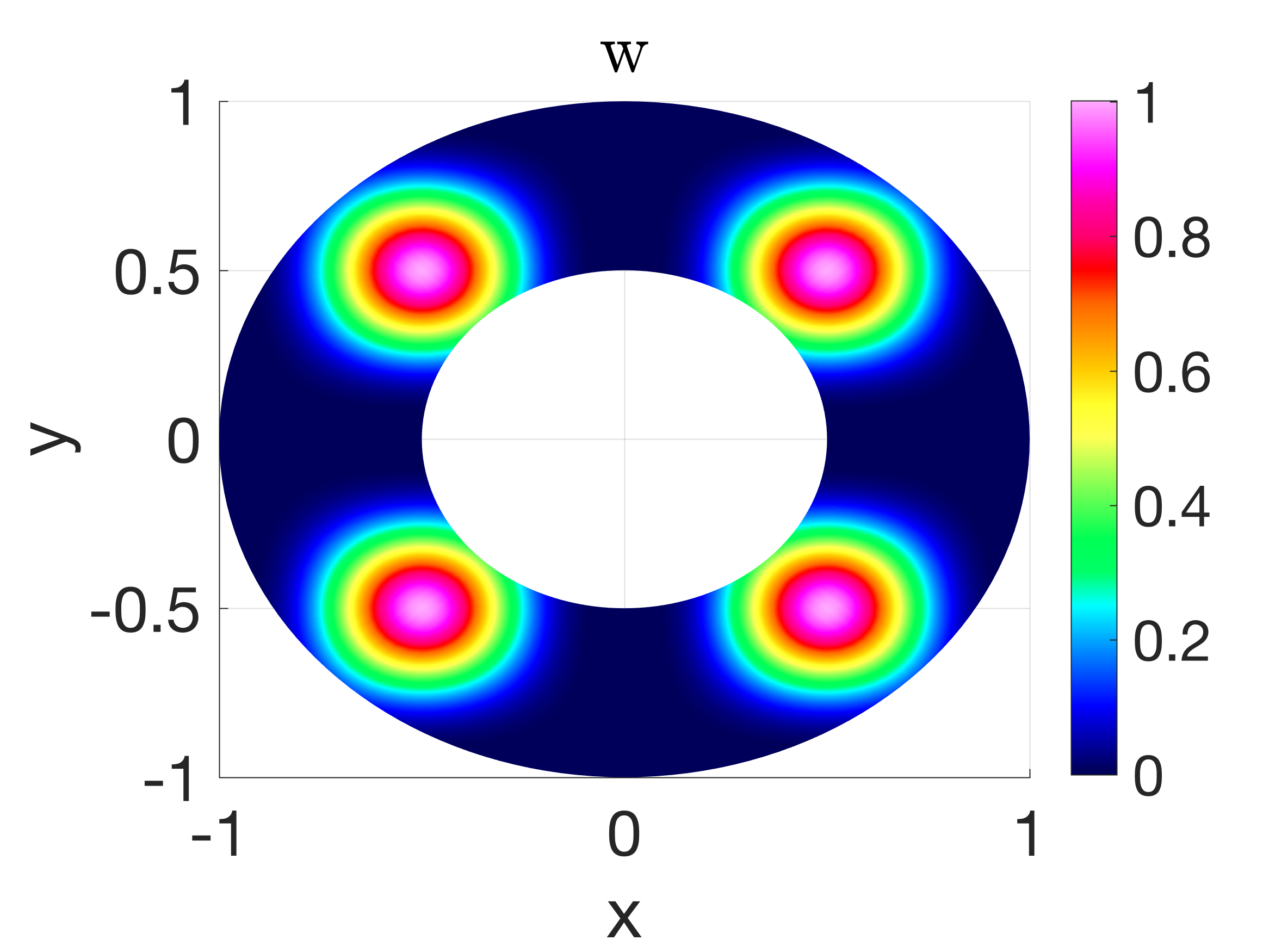
Figure 3: Contour plots of the computed displacement $w$ on grid ${\mathcal{G}}_{160}$ when $\text{t}=1$. The solution presented for the square plate are solved using the PC22 scheme subject to the free boundary conditions, while the plot for the annular plate is generated from the NB2 scheme with simply supported boundary conditions. Results obtained using either algorithm are similar regardless of the boundary conditions.

Clamped

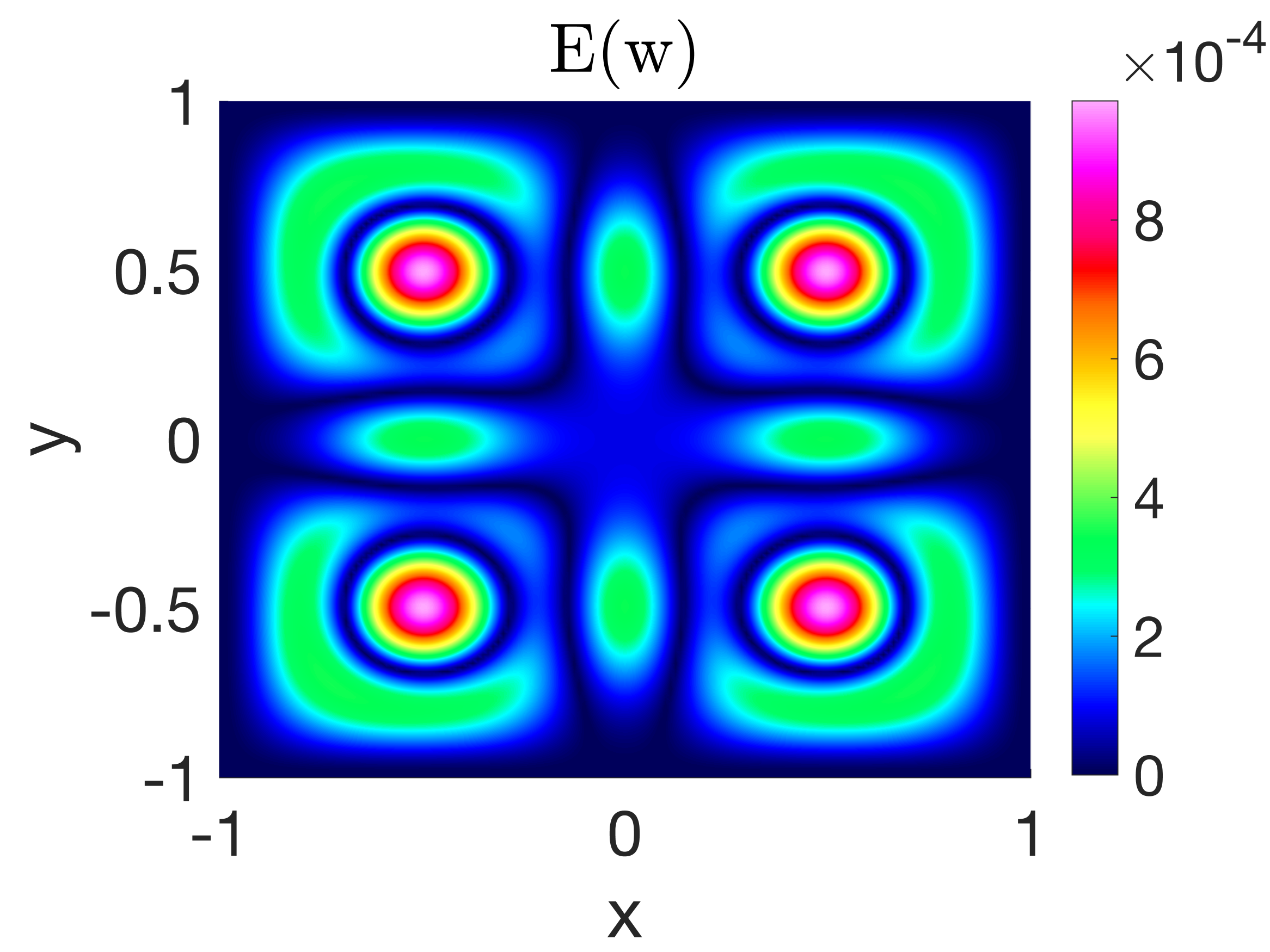
Simply Supported

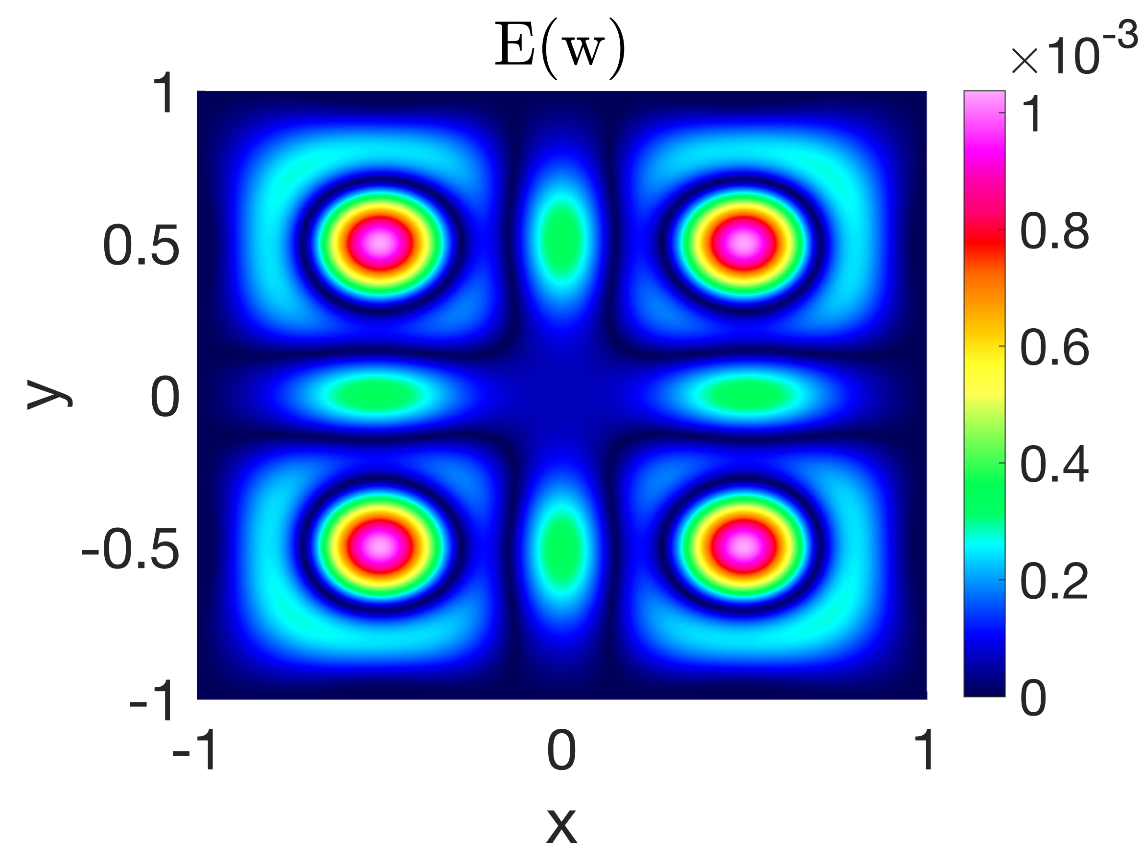
Free

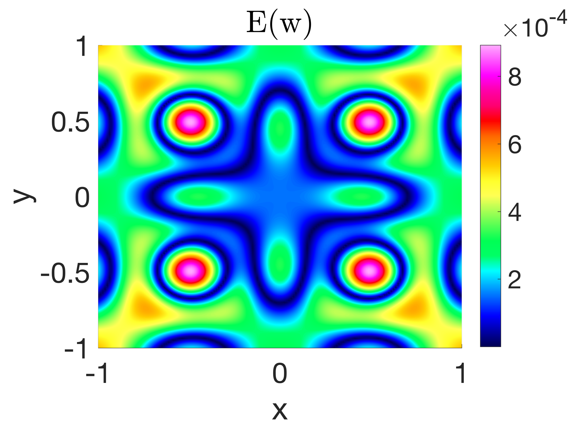
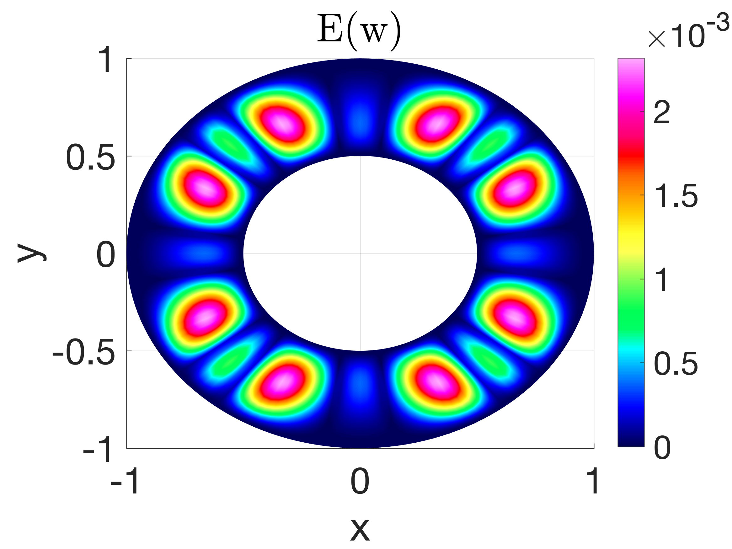
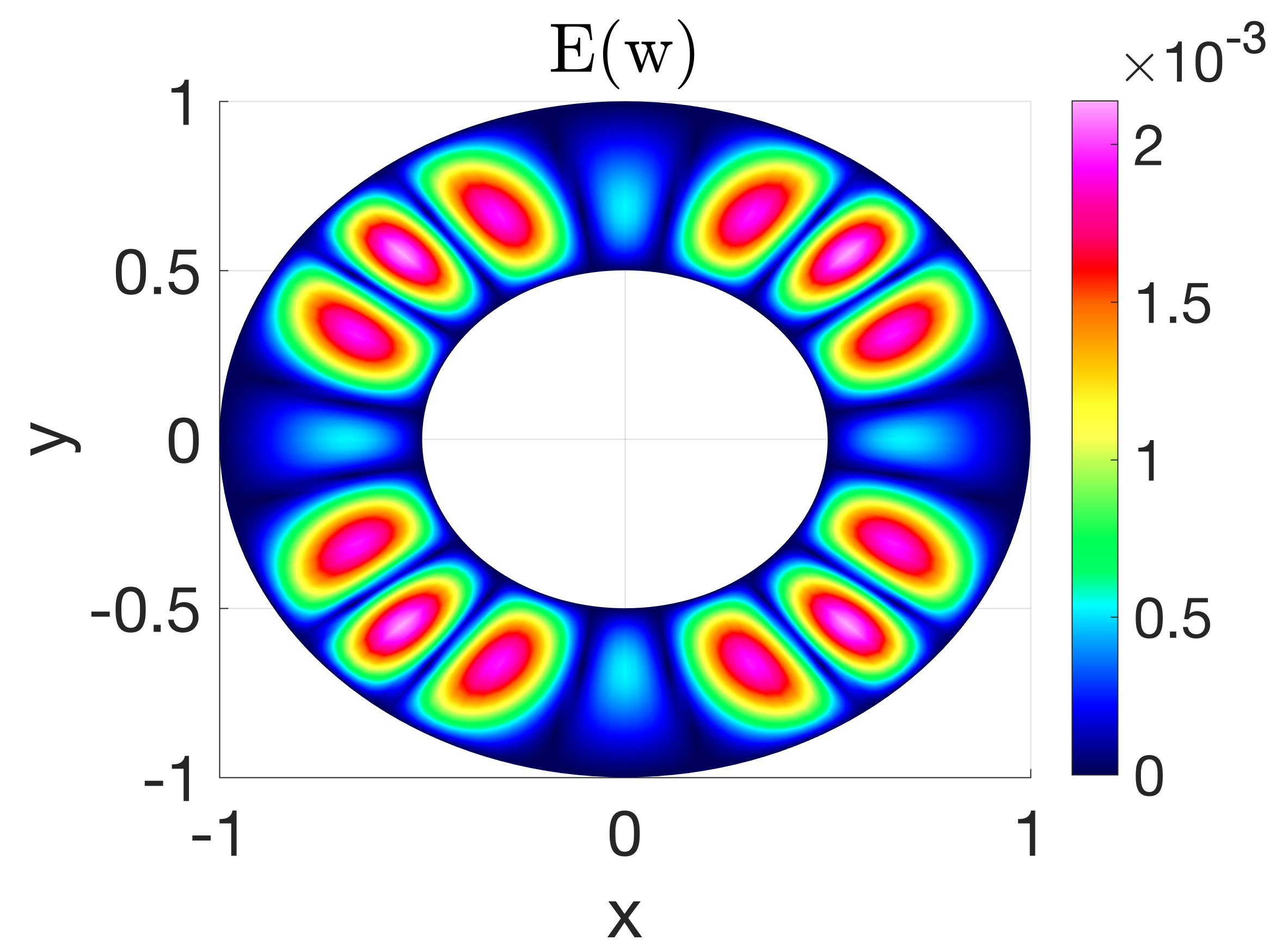
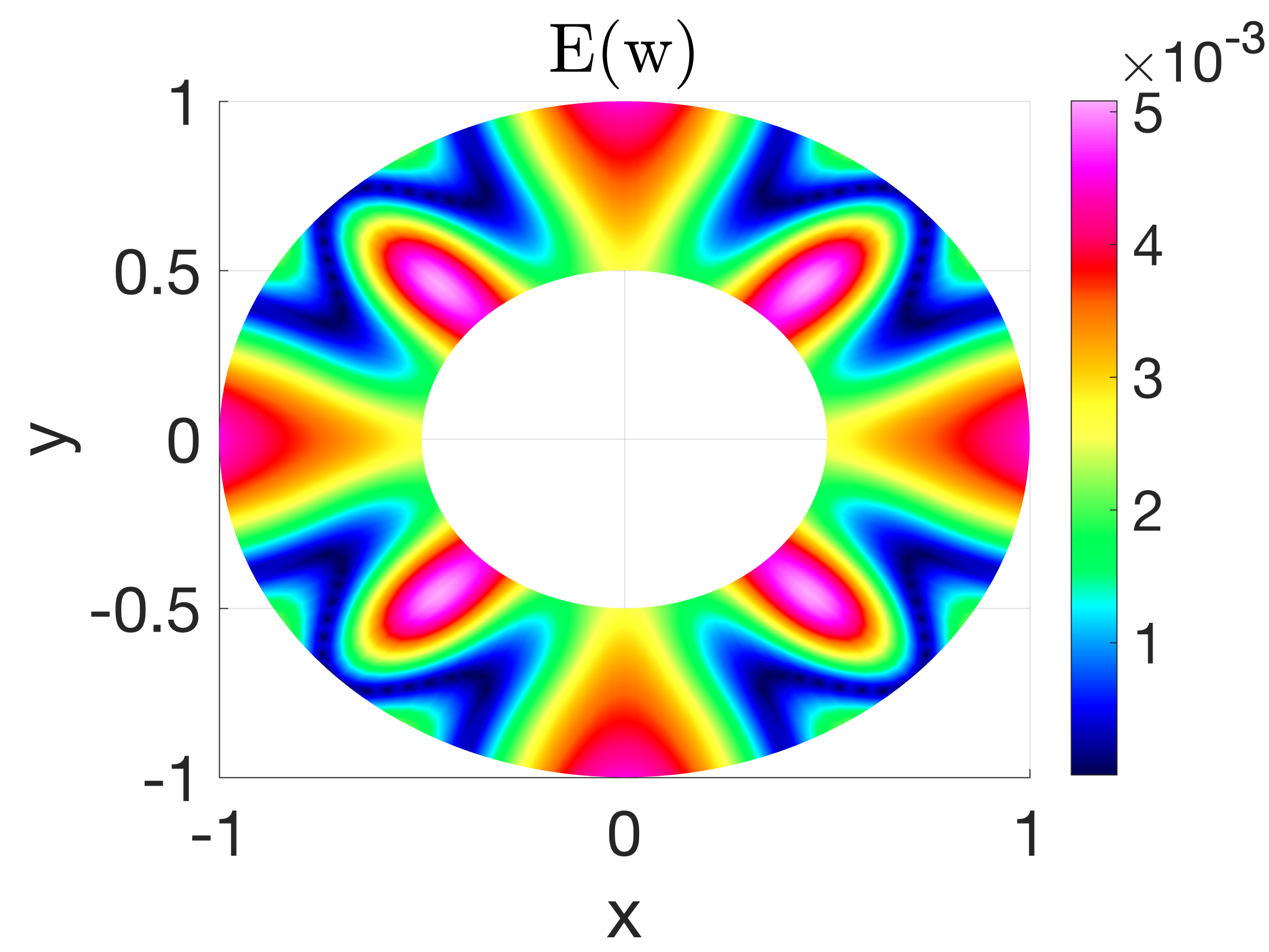
Figure 4: Contour plots showing the errors of the numerical solutions for the displacement $w$ with various boundary conditions when $\text{t}=1$. Results shown here are obtained on grid ${\mathcal{G}}_{160}$ using the PC22 method for the square plate and the NB2 method for the annular plate.

Given initial conditions from the exact solution at $t=0$, we solve the test problem to $t=1$ on a sequence of refined grids ${\mathcal{G}}_{N}$, where $N=10\times 2^{j}$ represents the number of grid points in each axial direction with $j$ ranging from $0$ through $4$. All the boundary conditions listed in (2)–(4) as well as both of the proposed schemes (i.e., PC22 and NB2) are considered, but we selectively present two of the numerical solutions obtained on the finest considered grid (i.e., ${\mathcal{G}}_{160}$) in Figure 3. In particular, the solution presented for the square plate is solved using the PC22 scheme subject to the free boundary conditions, while the plot for the annular plate is generated from the NB2 scheme with simply supported boundary conditions. We note that numerical solutions for the other cases are similar, since the test problem is designed to have the same exact solution (25).

Let $E(w)=|w_{\mathbf{i}}(t)-w_{e}(\mathbf{x}_{\mathbf{i}},t)|$ denote the error function of a numerical solution $w_{\mathbf{i}}(t)$, and we show in Figure 4 the contour plots of $E(w)$ on ${\mathcal{G}}_{160}$ to demonstrate the accuracy of our schemes for all the boundary conditions. Results shown for the square plate are obtained using the PC22 scheme, and those for the annular plate are solved with the NB2 scheme. We observe that the numerical solutions subject to all the boundary conditions are accurate in the sense that the errors are small and smooth throughout the domain including the boundaries. Errors for all the other cases behave similarly, so their plots are omitted here to save space.

Figure 5: Convergence rates of $w$ for both the square ($\Omega_{S}$) and the annular ($\Omega_{A}$) plates subject to all the boundary conditions are presented. The upper panel of plots show the results of the square plate, and the lower panel illustrates the results of the annular plate. The errors for both numerical methods (PC22 and NB2) are computed at $t=1$ and measured in the maximum norm.

Convergence studies for both the square and annular plates subject to all the boundary conditions are performed for the numerical results obtained on the sequence of grids ${\mathcal{G}}_{N}$’s using both numerical methods. We plot the maximum norm errors $||E(w)||_{\infty}$ against the grid size together with a second-order reference curve in log-log scale to reveal the order of accuracy. In the top row of Figure 5, we show the results for the square plate; and in the bottom row of the same figure, we show the results for the annular plate. For all the boundary conditions and both of the numerical schemes, we observe the expected second-order accuracy regardless of the plate shape.

5.2 Vibration of plates

Mechanical vibrations are problems of great interest in engineering and material sciences. For a thin plate-like structure, a 2D plate theory is capable of giving an excellent approximation to the actual 3D motion. The vibration of a plate can be caused either by displacing the plate from its stress-free state or by exerting an external forcing, where the former is referred to as free vibration and the latter is called forced vibration. Among the numerous plate models, the Kirchhoff-Love theory is most commonly used. To further validate the numerical properties of the proposed schemes, we consider the vibration problems of the generalized Kirchhoff-Love plate (1), which include the study of natural frequencies and mode shapes of vibration, and propagating or standing waves in the plate.

5.2.1 Vibration with known analytical solutions

The classical Kirchhoff-Love plate with some simple specifications can be solved analytically. We consider a thin plate on a rectangular domain (i.e., $\Omega=[0,L]\times[0,H]$). Analytical solutions to the classical Kirchhoff-Love plate equation subject to simply supported boundary conditions (3) are available for both the free and forced vibration cases. We solve each case numerically and compare our approximations with the analytical solutions to reveal the stability and accuracy of our schemes.

$\bullet$ Free vibration. Consider the free vibration case; i.e., the forcing function in (1) is zero ($F(\mathbf{x},t)\equiv 0$). In this case, the governing equation can be analytically solved using separation of variables or Fourier transformation. Let $A_{mn}$ and $B_{mn}$ denote the coefficients to be determined by the initial conditions and the orthogonality of Fourier components, then the general solution to this simple plate can be expressed as the following infinite series,

(26) $$w(\mathbf{x},t)=\sum_{m=1}^{\infty}\sum_{n=1}^{\infty}\sin\frac{m\pi x}{L}\sin\frac{n\pi y}{H}(A_{mn}\cos\omega_{mn}t+B_{mn}\sin\omega_{mn}t),$$

where the natural frequencies of vibration for this plate is found to be

(27) $$\omega_{mn}={\pi^{2}}\left(\frac{m^{2}}{L^{2}}+\frac{n^{2}}{H^{2}}\right)\sqrt{\frac{D}{\rho h}}.$$

Standing wave test problems can be constructed by specifying modes of vibration as the given functions for the initial conditions (5); namely,

(28) $$w_{0}(\mathbf{x})=\sin\frac{m\pi x}{L}\sin\frac{n\pi y}{H},\leavevmode\nobreak\ \text{and}\leavevmode\nobreak\ v_{0}(\mathbf{x})=0.$$

Enforcing the above initial conditions on the general solution (26), we deduce the exact standing wave solution for each 2-tuple $(m,n)$,

(29) $$w_{e}(\mathbf{x},t)=\sin\frac{m\pi x}{L}\sin\frac{n\pi y}{H}\cos\omega_{mn}t.$$

We solve the standing wave test problem for a few modes to validate our numerical schemes. That is to say, we specify the initial conditions (28) with various values of $(m,n)$, and compare the numerical approximations with the exact solution (29). For simplicity, the rectangular domain is restricted to a unit square in the computations; namely, we set $L=H=1$ in $\Omega=[0,L]\times[0,H]$. The parameters for this test are specified as $\rho h=2.7$, $K_{0}=0$, $T=0$, $D=6.4527$, $K_{1}=0$, $T_{1}=0$ and $\nu=0.33$. Note that this is a classical Kirchhoff-Love model because only the bending dynamics is accounted for (namely, $D\neq 0$). Both of the proposed schemes are used to conduct numerical simulations, but only the results of the PC22 scheme are presented in Figure 6 since the other scheme produces comparable results. In Figure 6, we show the contour plots of the displacement $w$ at $t=1$ for a few $(m,n)$-tuples. In the plots, we also show the zero contours, which represent the nodal lines of the standing wave solutions. It is clear that the patterns of these nodal lines exhibited in the numerical solutions resemble those of the corresponding modes of vibration used in the initial conditions (28).

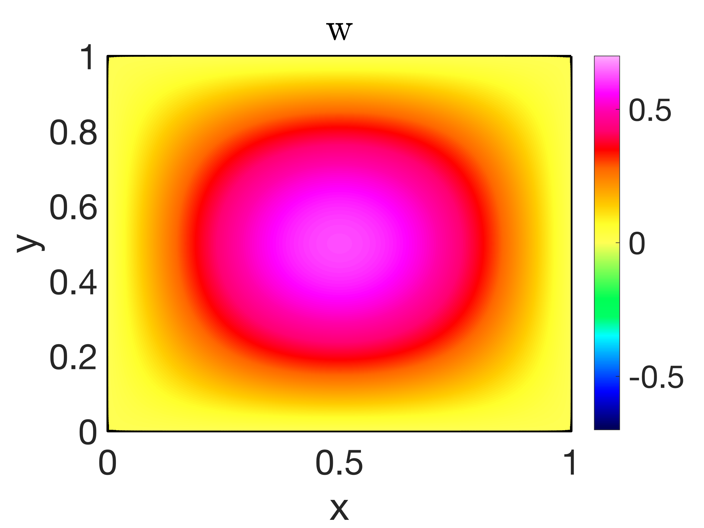
(a) $m=1,n=1$

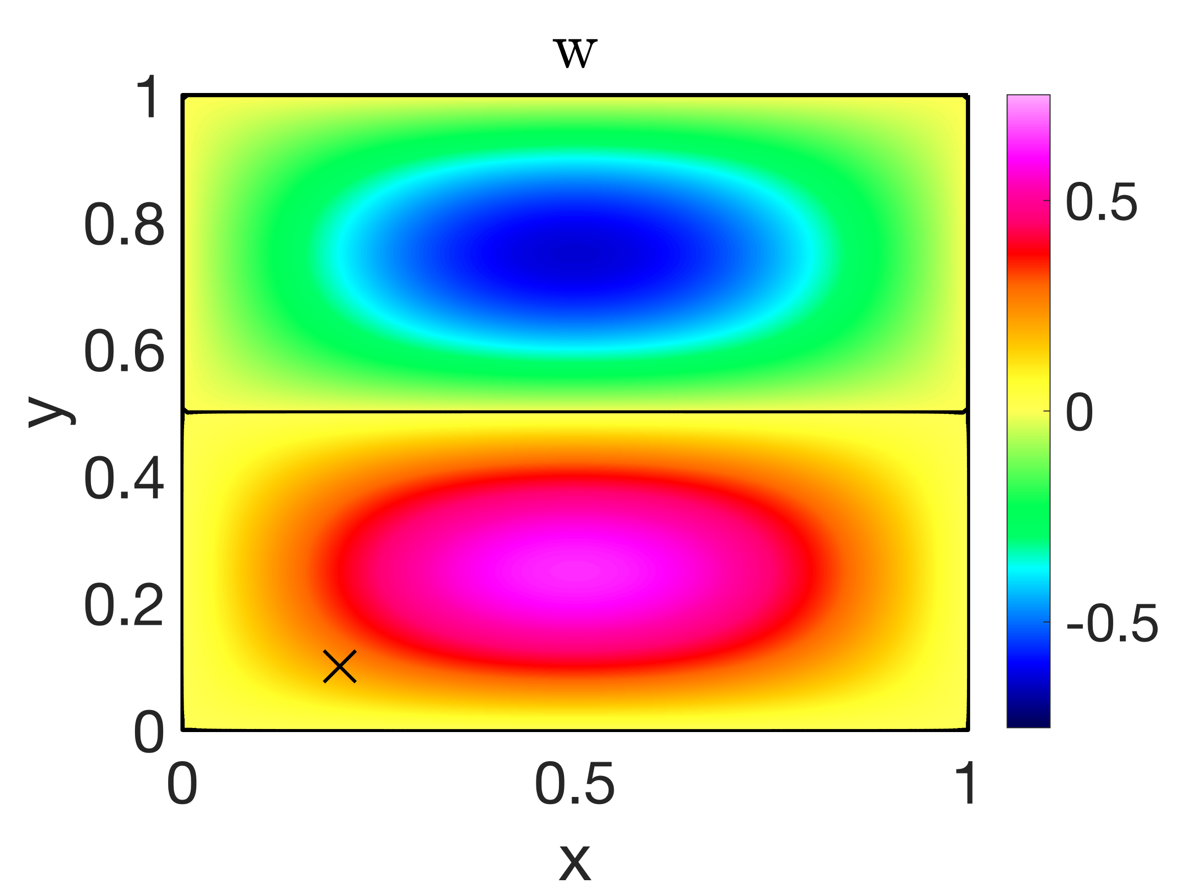
(b) $m=1,n=2$

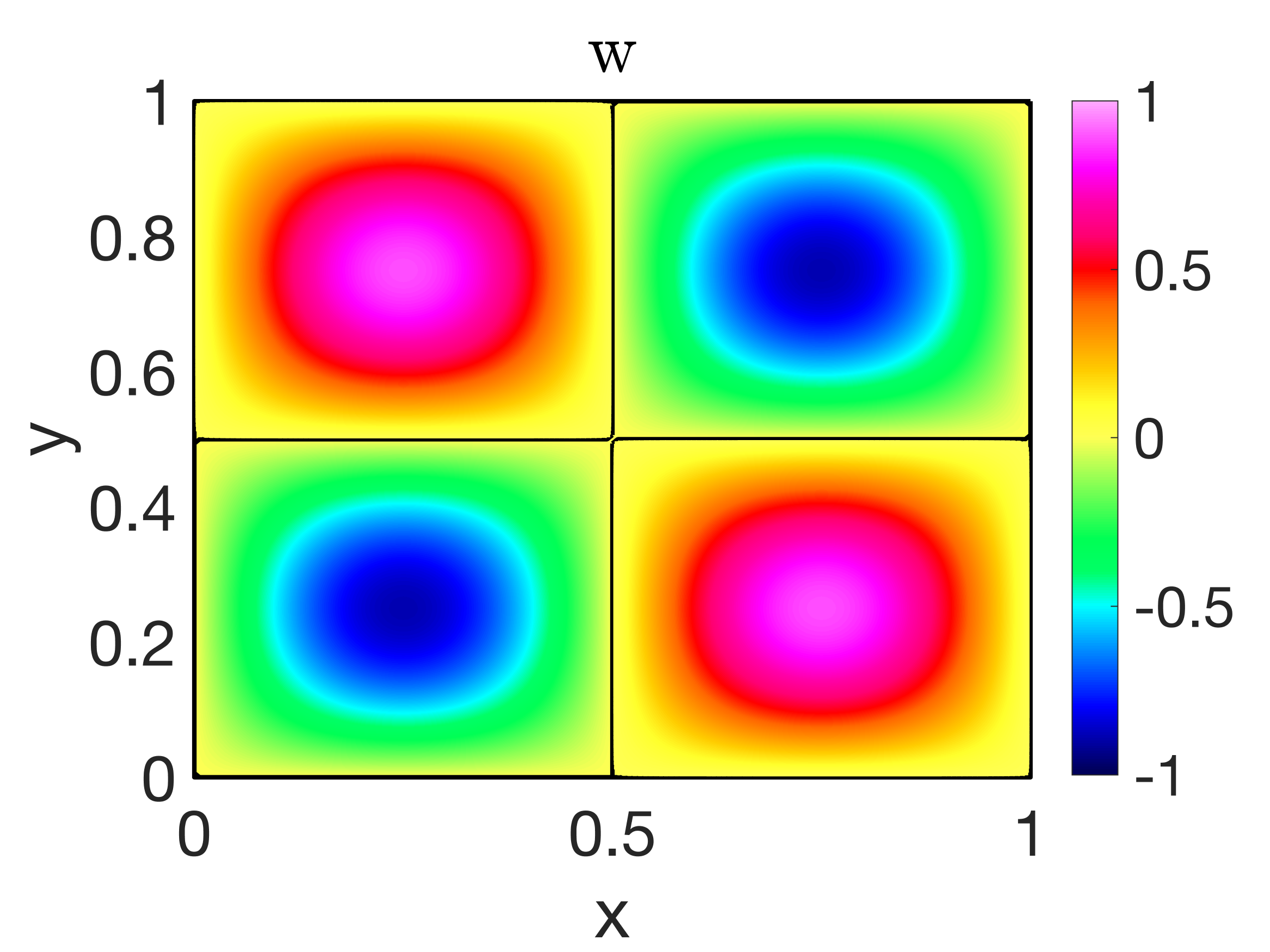
(c) $m=2,n=2$

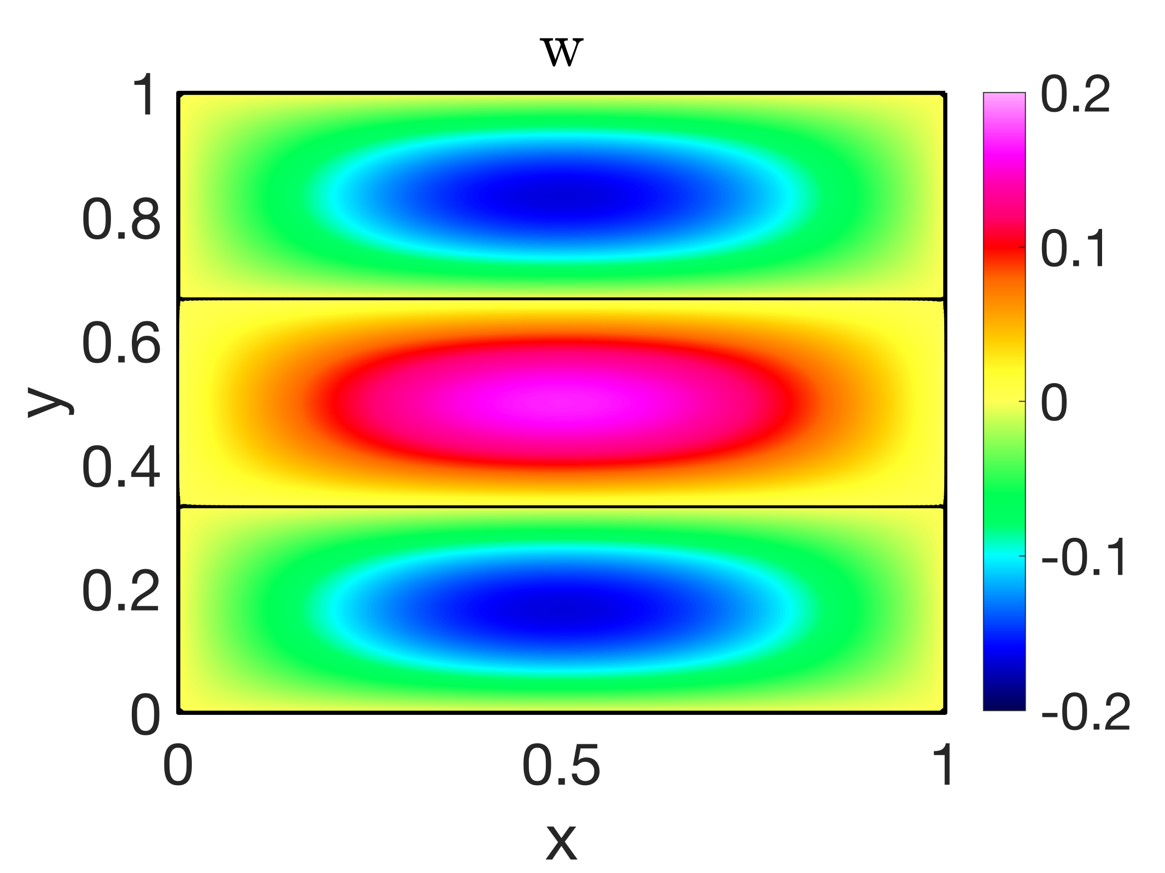
(d) $m=1,n=3$

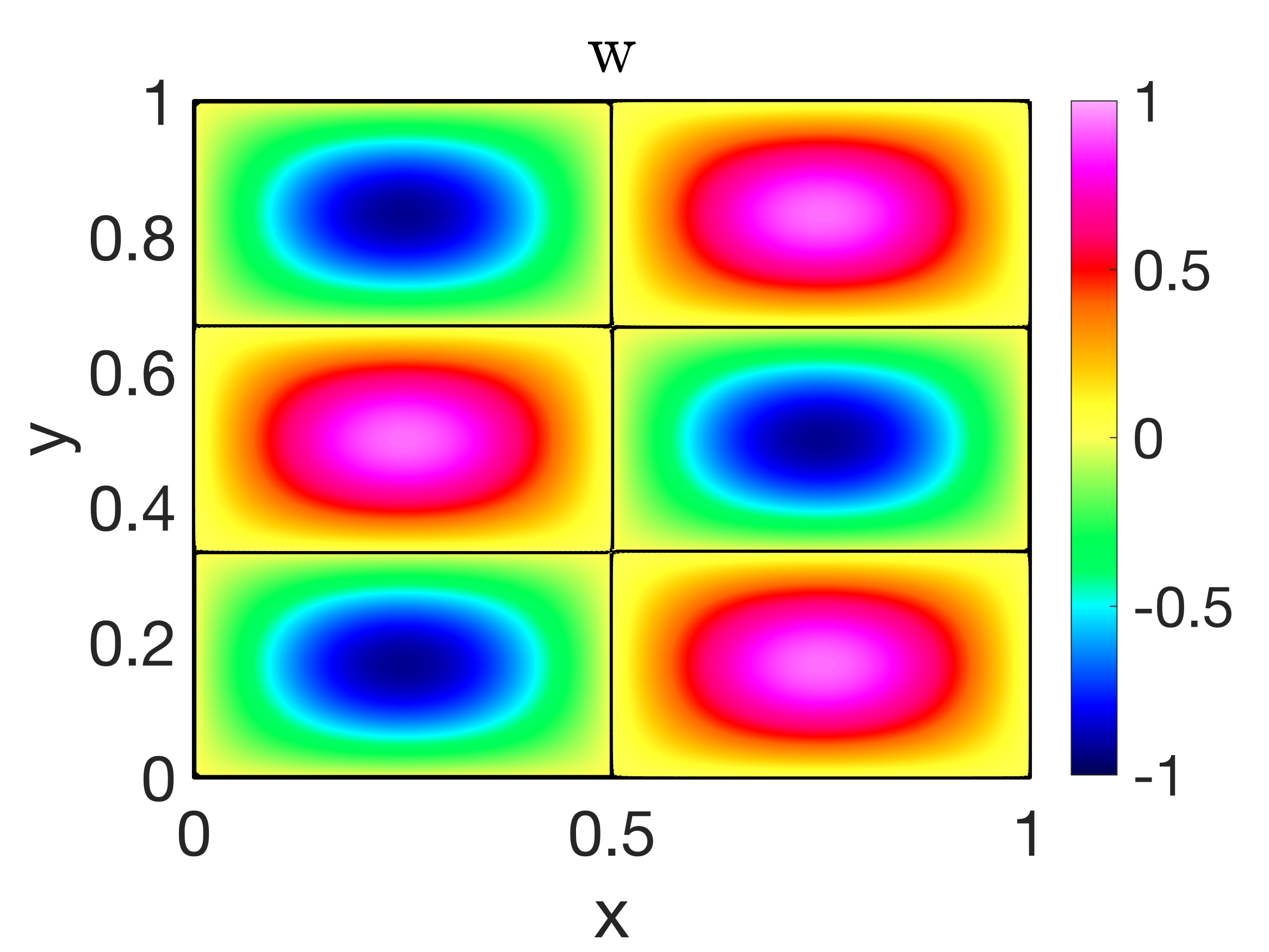
(e) $m=2,n=3$

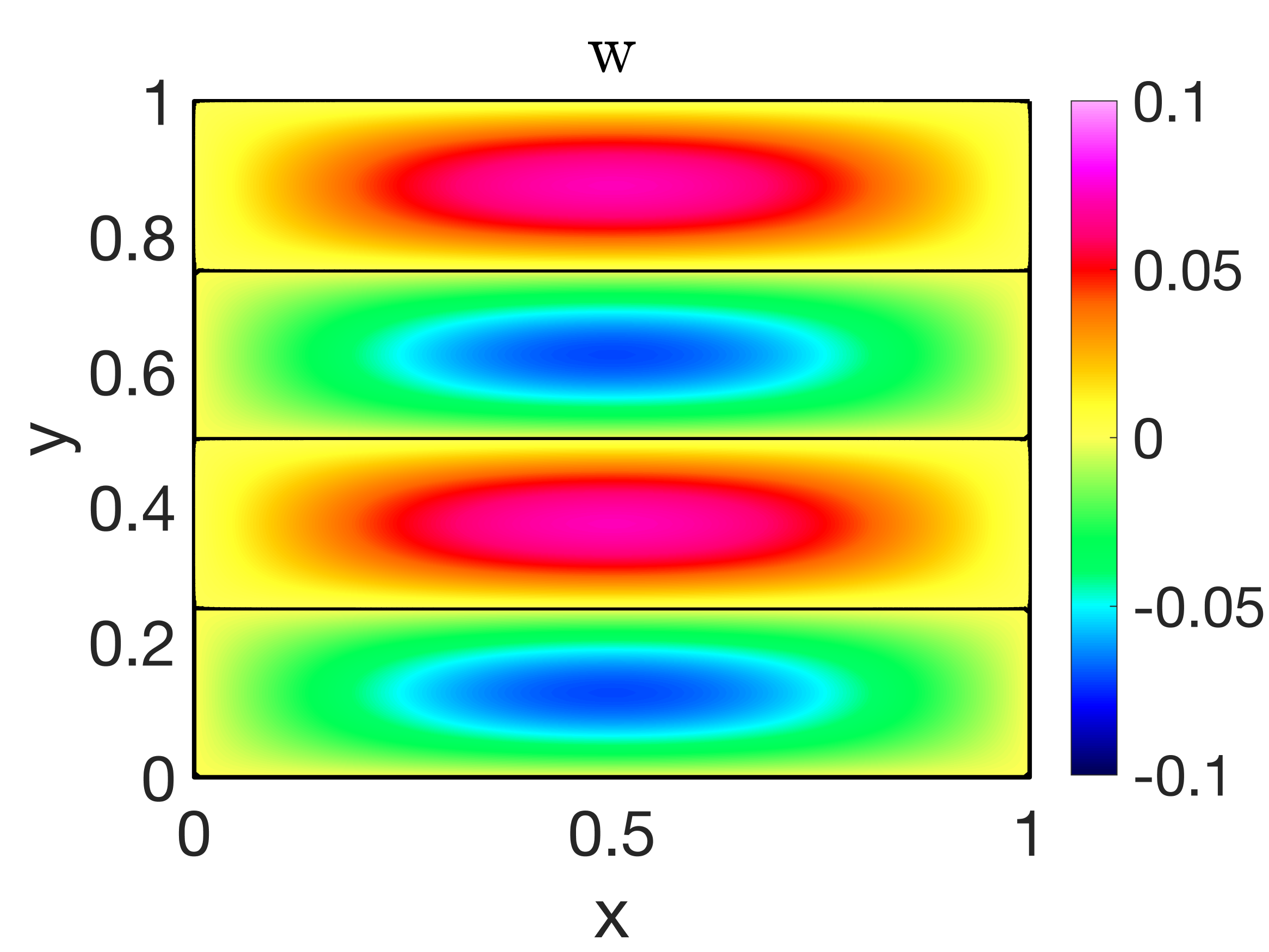
(f) $m=1,n=4$

Figure 6: Standing wave solutions with the nodal lines at time $t=1$ for some $(m,n)$ values. Simulations are performed using the PC22 scheme on grid ${\mathcal{G}}_{160}$. Results obtained using NB2 scheme are similar.

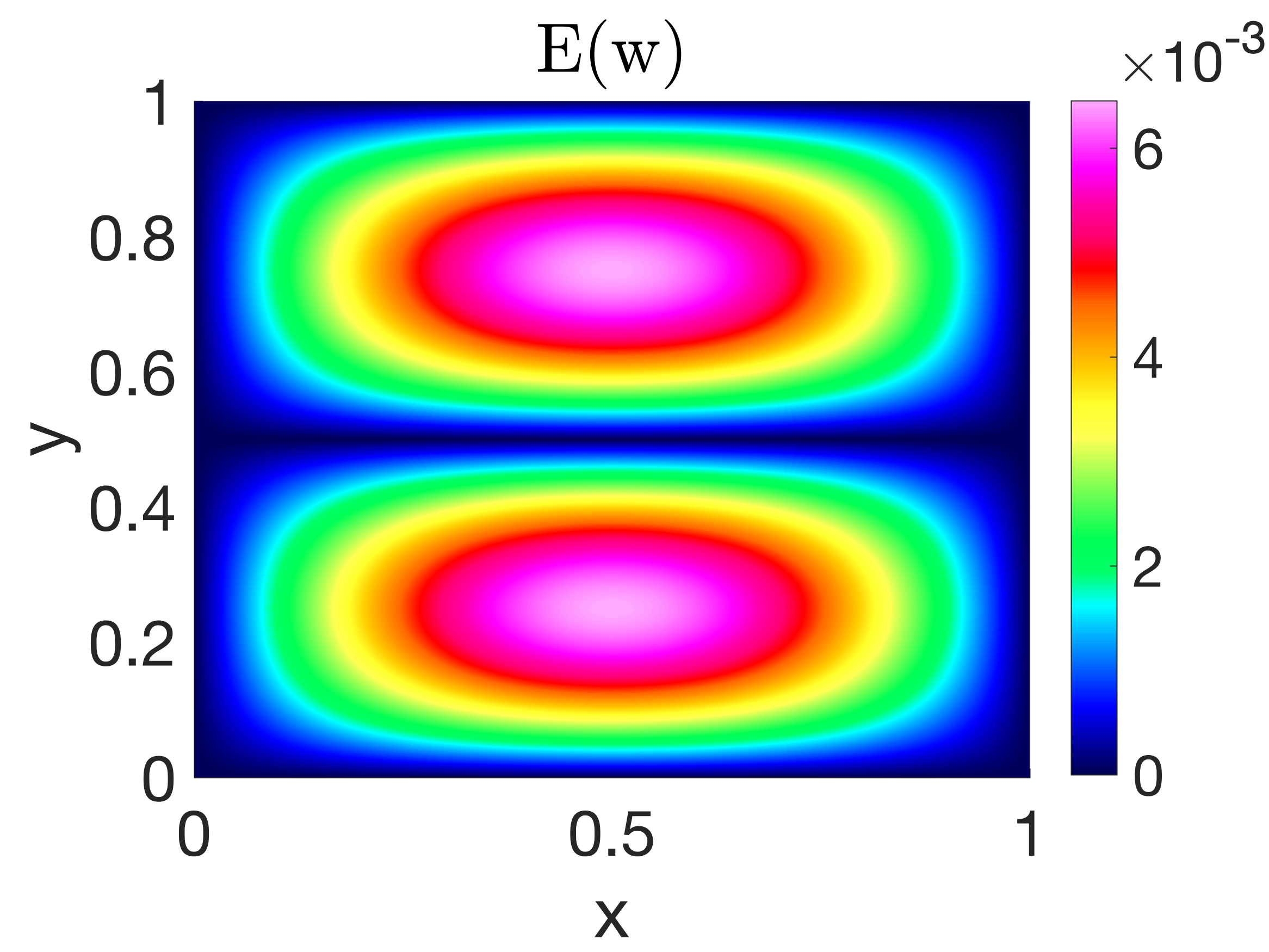
Error

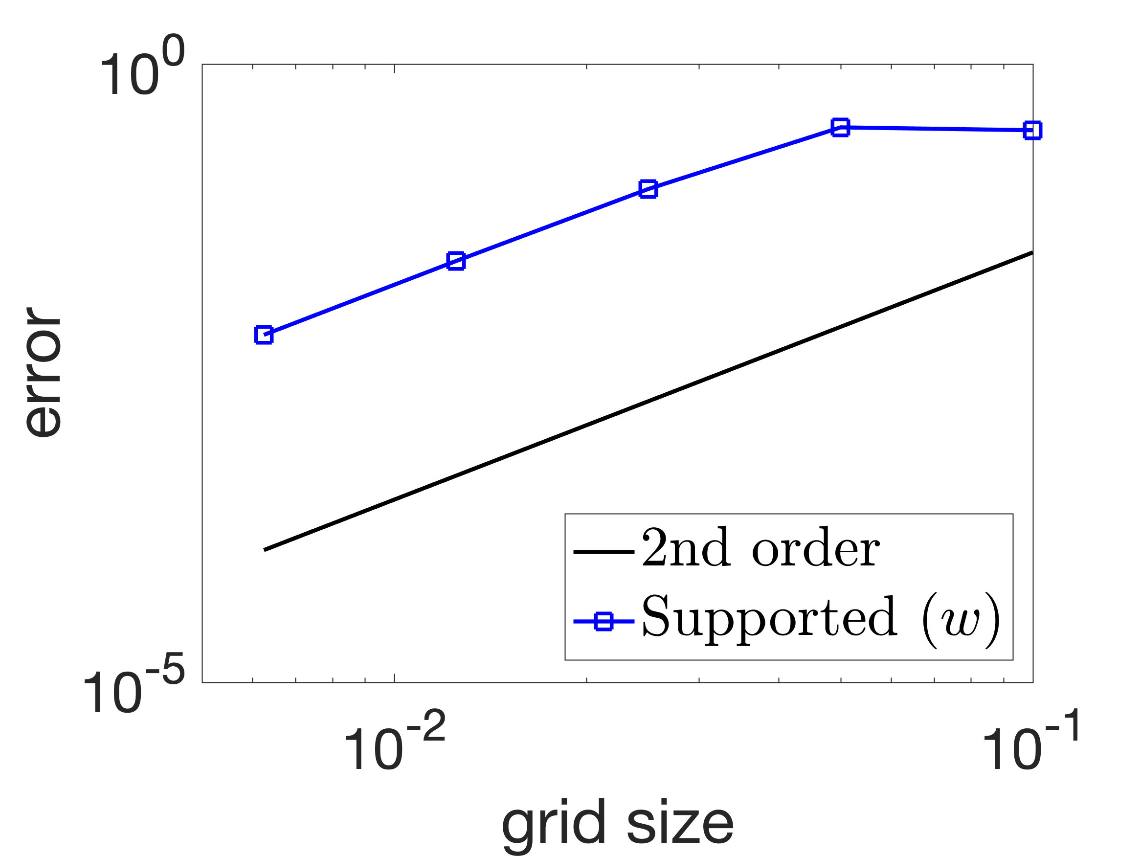
Convergence rate

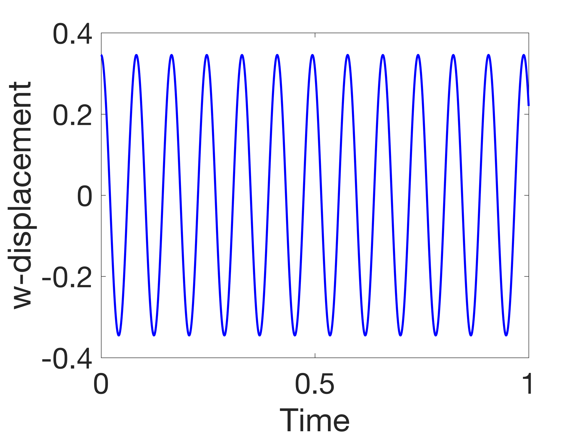
Displacement at $\mathbf{x}_{p}$

Figure 7: More results for the case with $m=1,n=2$. Left: the error plot of the displacement $w$ at $t=1$. Middle: the convergence rate of $w$. Right: displacement at point $\mathbf{x}_{p}$; the probed location is marked by a cross symbol in Figure 6(b).

Given that the exact solutions for these standing waves are available in (29), it is possible for us to perform mesh refinement studies to show the accuracy and the convergence of the numerical solutions. In Figure 7, we present more results for the case with $m=1$ and $n=2$, which include the error of $w$ at $t=1$ plotted in the left image, the convergence rate of $w$ shown in the middle image, and the evolution of $w$ at a probed location depicted in the right image. The probed location is $\mathbf{x}_{p}=(0.2,0.1)$, which is marked by a cross symbol in Figure 6(b). The error and convergence rate plots confirm that the scheme is accurate and the rate of convergence is second order.

The evolution of $w$ at a point, as the one shown in the right image of Figure 7, demonstrates how the standing wave solutions oscillate in time. From the evolution curve, we can estimate the frequency of oscillation by measuring the number of cycles per unit time, which should match up with the natural frequency of the plate. As another indication of the accuracy of our proposed schemes, we compare the numerically estimated frequencies with the natural frequencies. Please note that the natural frequencies defined in (27) are actually angular frequencies that measure the number of oscillations in $2\pi$ units of time. For comparison, we use the ordinary frequency (measured in hertz) that is given by $f_{mn}=\omega_{mn}/(2\pi)$. We track the evolution of the displacement at $\mathbf{x}_{p}=(0.2,0.1)$ for the modes that correspond to the first 9 natural frequencies, and estimate the frequencies of oscillation from the evolution curves. The frequencies inferred from the numerical solutions on grid ${\mathcal{G}}_{160}$ are summarized in Table 1. We can see that, for both numerical methods, the discrepancies between the estimated frequencies and $f_{mn}$ are small for all the examined cases.

$(m,n)$	${f_{mn}}$	PC22 scheme		NB2 scheme
		frequency (est.)	error (%)	frequency (est.)	error (%)
$(1,1)$	$4.8567$	$4.8565$	$0.0037\%$	$4.8541$	$0.0540\%$
$(1,2)$	$12.1417$	$12.1403$	$0.0112\%$	$12.1359$	$0.0480\%$
$(2,2)$	$19.4267$	$19.4242$	$0.0130\%$	$19.4203$	$0.0331\%$
$(1,3)$	$24.2834$	$24.2769$	$0.0268\%$	$24.2691$	$0.0589\%$
$(2,3)$	$31.5684$	$31.5608$	$0.0239\%$	$31.5544$	$0.0443\%$
$(1,4)$	$41.2817$	$41.2617$	$0.0485\%$	$41.2344$	$0.1146\%$
$(3,3)$	$43.7100$	$43.6975$	$0.0286\%$	$43.6542$	$0.1277\%$
$(2,4)$	$48.5667$	$48.5455$	$0.0436\%$	$48.4883$	$0.1615\%$
$(3,4)$	$60.7084$	$60.6821$	$0.0434\%$	$60.5840$	$0.2048\%$

Table 1: Comparison between the frequencies estimated from the numerical solutions on grid ${\mathcal{G}}_{160}$ and the first $9$ natural frequencies. Discrepancies are measured using the percentage of the relative errors.

$\bullet$ Forced vibration. Now, we consider the vibration of the classical Kirchhoff-Love plate driven by a time-dependent sinusoidal force $F(\mathbf{x},t)=F_{0}\sin(\xi t)$, where $F_{0}$ and $\xi$ are constants for the magnitude and frequency of the sinusoidal force. The plate is assumed to be undeformed and at rest initially; that is, $w_{0}=v_{0}=0$. Using method of eigenfunction expansion, we find the exact solution to the forced vibration problem,

(30) $$w(x,y,t)=\sum_{m=1}^{\infty}\sum_{n=1}^{\infty}\sin\frac{m\pi x}{L}\sin\frac{n\pi y}{H}T_{mn}(t),$$

where the time-dependent coefficient $T_{mn}(t)$ is given by

$$T_{mn}(t)=\frac{2F_{0}\left(1-\cos(m\pi)\right)\left(1-\cos(n\pi)\right)}{\rho hmn\pi^{2}\omega_{mn}}\left(\frac{\sin(\xi t)+\sin(\omega_{mn}t)}{\xi+\omega_{mn}}-\frac{\sin(\xi t)-\sin(\omega_{mn}t)}{\xi-\omega_{mn}}\right).$$

For numerical test, we consider a classical Kirchhoff-Love plate with the parameters specified as $\rho h=1$, $K_{0}=0$, $T=0$, $D=0.1$, $K_{1}=0$, $T_{1}=0$ and $\nu=0.3$ on a rectangular domain $\Omega=[0,0.4]\times[0,0.2]$; namely $L=0.4$ and $H=0.2$. The magnitude and frequency of the driving force are set as $F_{0}=1000$ and $\lambda=40$. This test problem is solved using both of the proposed schemes on a uniform Cartesian grid with grid spacings $h_{x}=h_{y}=1/300$. The numerical results are compared with an analytical solution truncated from the exact solution (30) by keeping 49 modes (i.e., $m=1,\dots,7$ and $n=1,\dots,7$).

Figure 8: Contour plots of the numerical solution (left) and the error (right) of $w$ at $t=1$. Results are obtained using the NB2 scheme on a uniform Cartesian grid with grid spacings $h_{x}=h_{y}=1/300$.

Figure 9: The displacement and velocity of the plate at point $\mathbf{x}_{p}=(0.2,0.1)$. Simulation is performed using the NB2 scheme on a uniform Cartesian grid with grid spacings $h_{x}=h_{y}=1/300$.

Both schemes perform comparably well and produce similar solutions, so we only show the one obtained with the NB2 schemes here. In Figure 8, the contour plots of the numerical solution of $w$ at $t=1$ and the error compared with the truncated exact solution are presented. To show the accuracy of the numerical results over time, we track the displacement $w$, as well the velocity $v$, at the point $\mathbf{x}_{p}=(0.2,0.1)$. The time evolution of the numerical displacement and velocity at $\mathbf{x}_{p}$ are plotted on top of the referenced analytical solutions in Figure 9; it is easily seen that our numerical results agree well with the analytical solution over time.

5.2.2 Vibration of the generalized Kirchhoff-Love plate

For the generalized Kirchhoff-Love model (1) that cannot be solved analytically, we numerically solve the frequency domain eigenvalue problem to identify the natural frequencies and modes of vibration for the plate, and then utilize the computed eigenvalues and eigenvectors to construct standing wave solutions. The nodal line patterns (i.e., Chladni figures) of the standing wave solutions obtained from our numerical simulations are compared against those solved from the eigenvalue problem for the validation of the numerical schemes.

Specifically, a square plate ($\Omega_{S}=[0,0.25]\times[0,0.25]$) and an annulus plate ($\Omega_{A}=\{\mathbf{x}:0.1\leq|\mathbf{x}|\leq 0.5\}$) are considered. For both plates, we assume the same parameters, $\rho h=1,K_{0}=2,T=1,D=2,K_{1}=0,T_{1}=0$, and $\nu=0.1$, noting that these parameters specify an undamped plate. On the edges of the plates, we impose the clamped boundary conditions (2) for square plate, and the simply supported boundary conditions (3) for the annular plate.

First, let’s consider the eigenvalue problem for the undamped plate on mesh $\Omega_{h}$,

(31) $${\mathcal{K}}_{h}\phi_{\mathbf{i}}=\lambda\phi_{\mathbf{i}},\leavevmode\nobreak\ \mathbf{x}_{\mathbf{i}}\in\Omega_{h},$$

where $\phi_{\mathbf{i}}=\phi(\mathbf{x}_{\mathbf{i}})$ is the mode function (or eigenfunction) for the eigenvalue $\lambda$. The definition of the difference operator ${\mathcal{K}}_{h}$ is given in (13). To get the eigenfunction-eigenvalue pairs $(\phi_{n}(\mathbf{x}),\lambda_{n})$, we numerically solve the eigenvalue problem (31) subject to the appropriate numerical boundary conditions; that is, clamped (7) for the square plate and supported (8) for the annular plate. The eigs function in MATLAB is used here. To save space, we put the results in Appendix A, where the nodal lines of the first 25 eigenmodes (with multiplicity) for the plates (square and annular) are presented in Figures 17 & 18. Note that, following the tradition in structural engineering, the values of natural frequencies, rather than the eigenvalues, are reported in the plots. The natural frequency corresponding to $\lambda_{n}$ is given by

$$f_{n}=\frac{1}{2\pi}\sqrt{\frac{\lambda_{n}}{\rho h}}.$$

$f_{11}=395.1906$

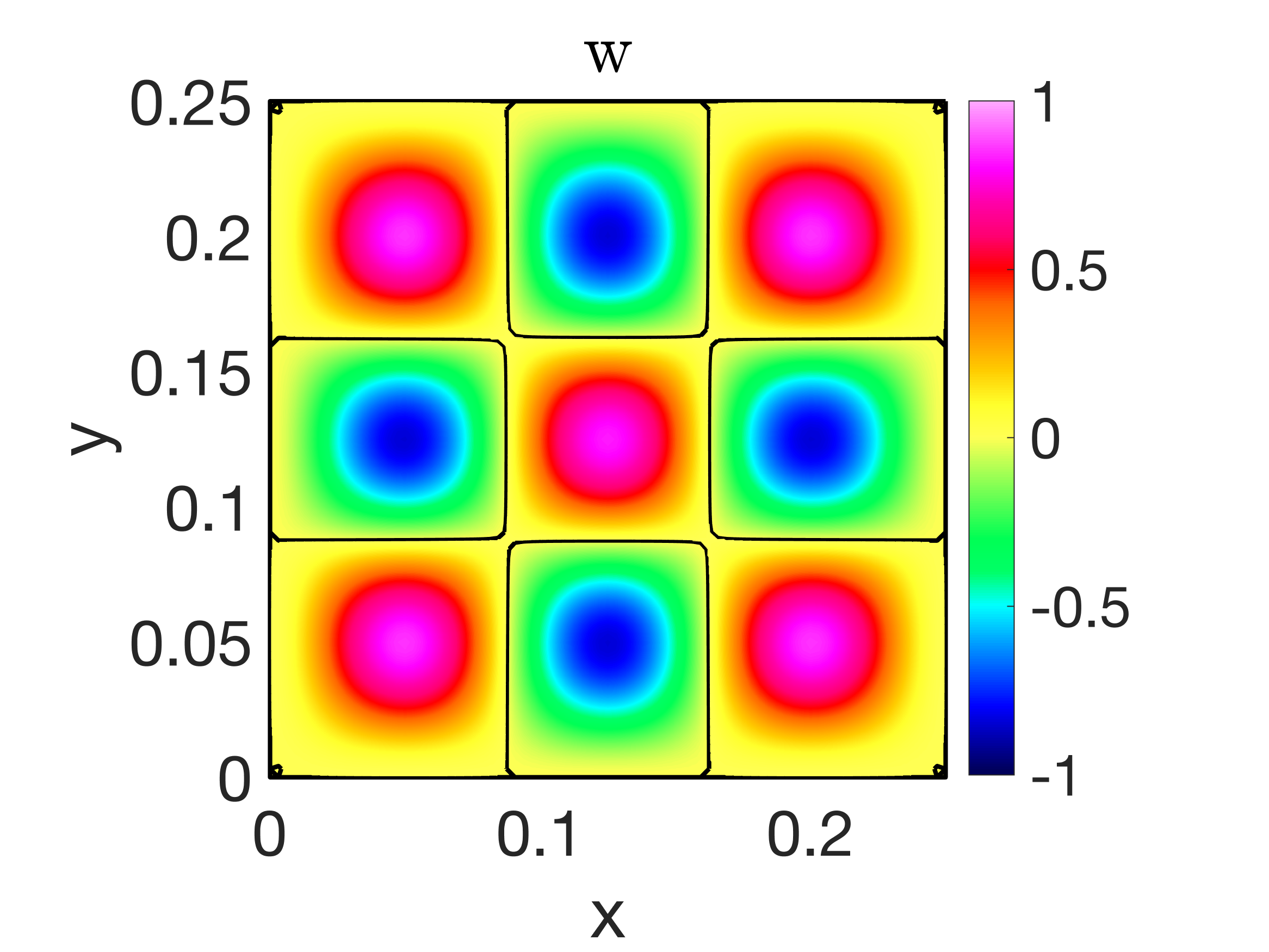
$f_{17}=553.9450$

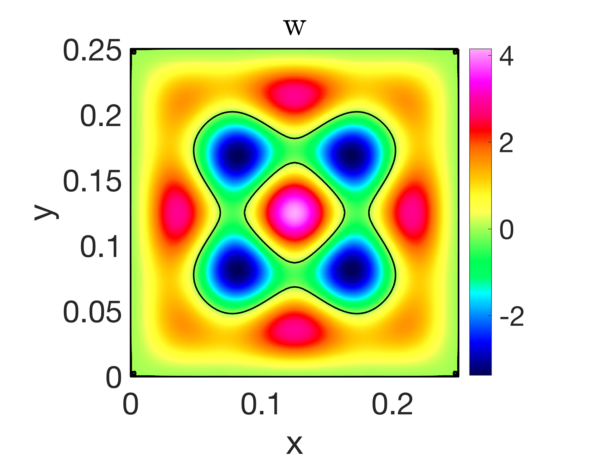
$f_{22}=705.9267$

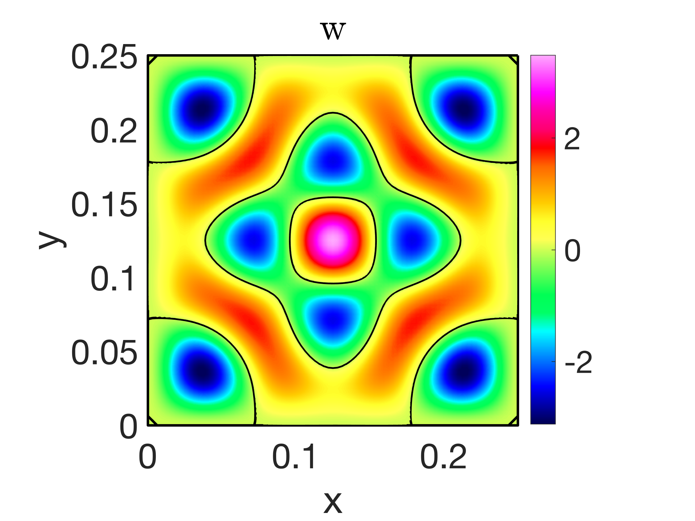
Figure 10: Standing waves in the square plate with clamped edges at time $t=1$ for three eigenvalue cases. Zero contour lines of the solutions are also plotted to indicate the nodal line patterns. Simulations are performed using the NB2 scheme on grid ${\mathcal{G}}_{80}$.

$f_{2}=8.8174$

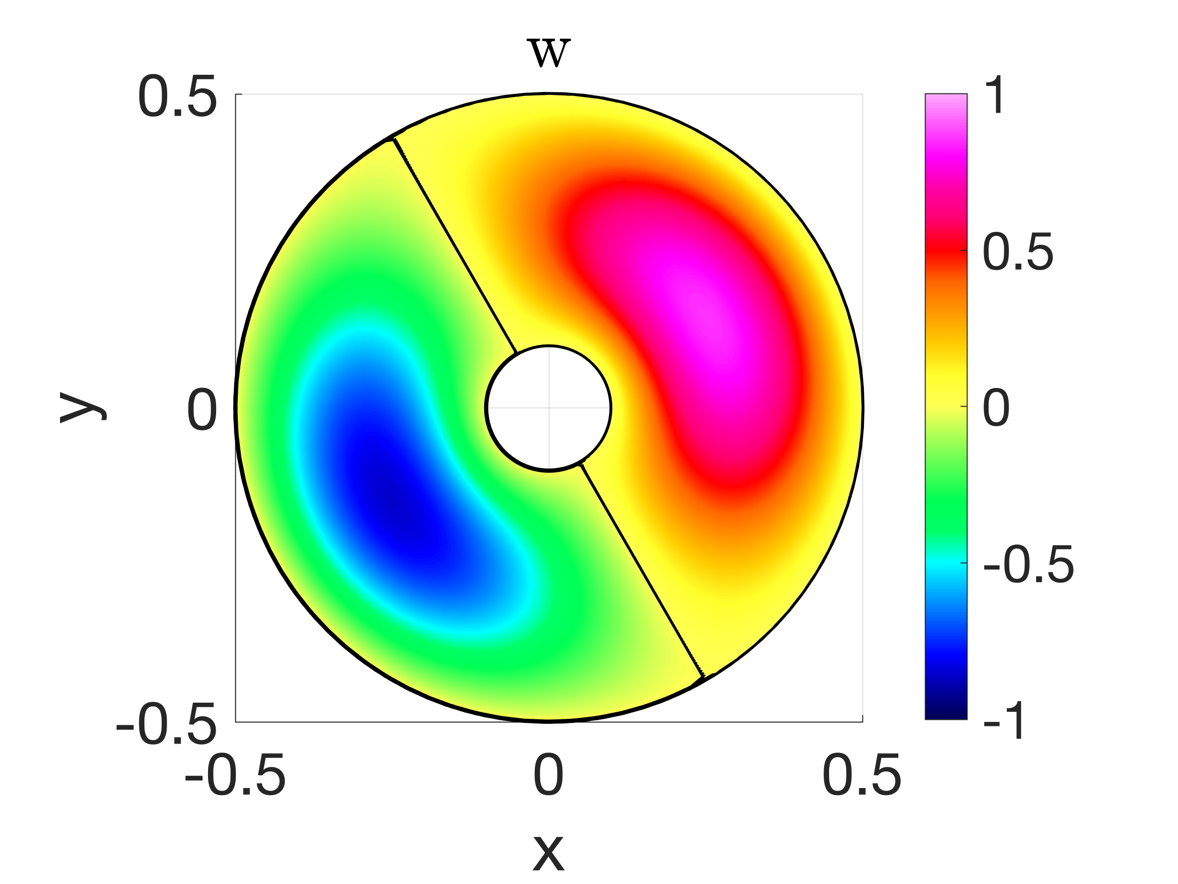
$f_{10}=28.9529$

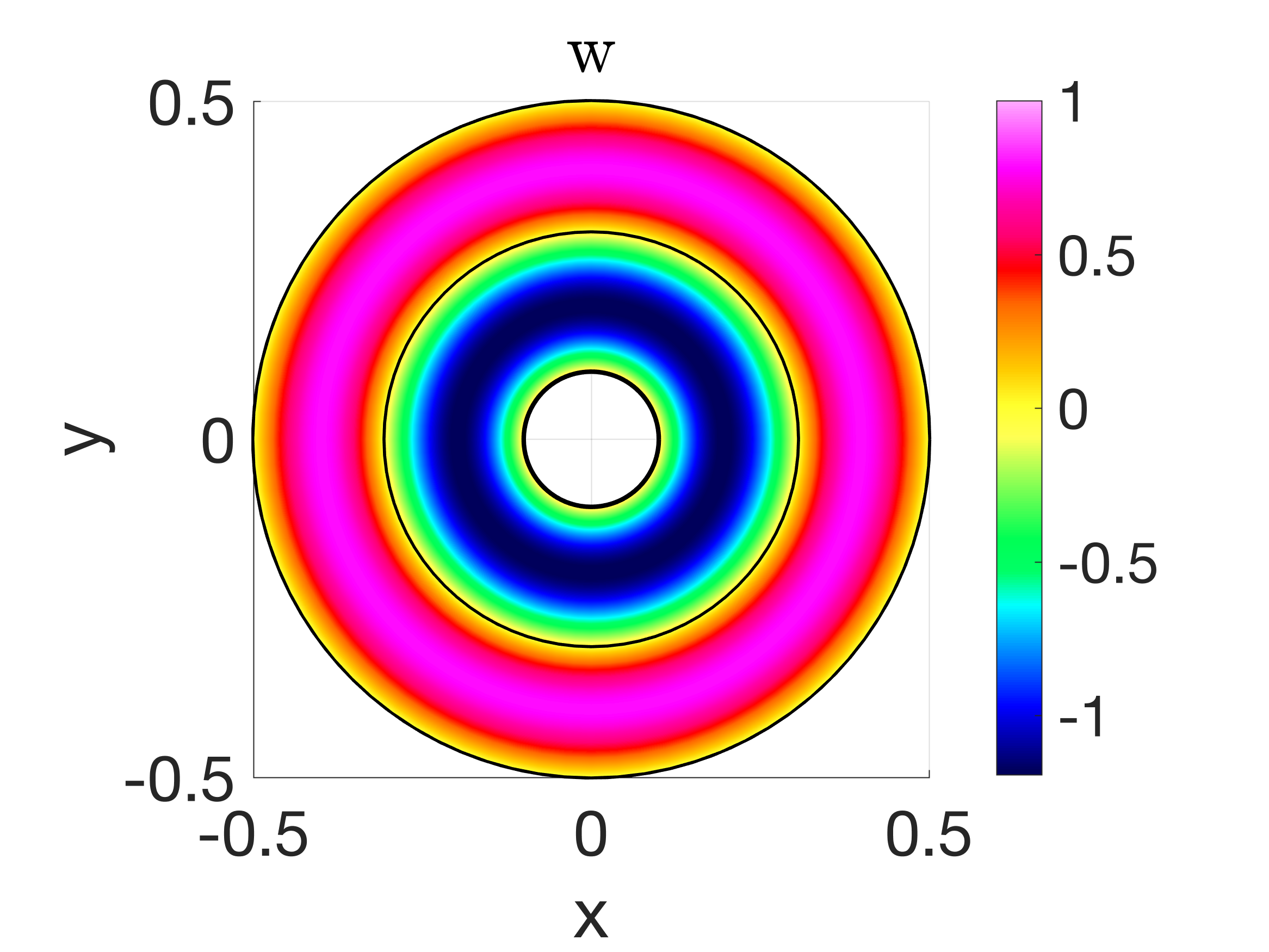
$f_{20}=43.8879$

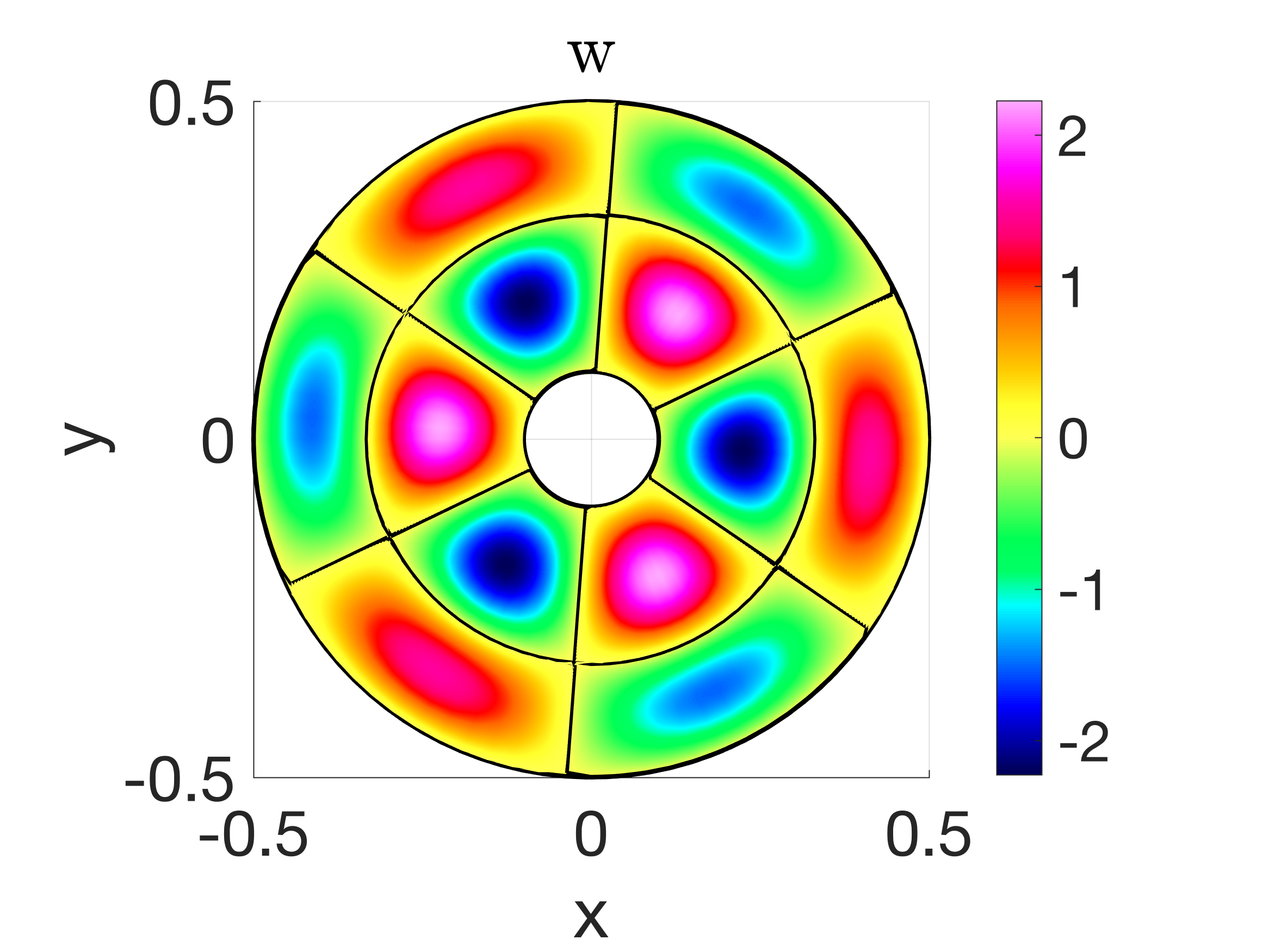
Figure 11: Standing waves in the annular plate with simply supported edges at time $t=1$ for three eigenvalue cases. Zero contour lines of the solutions are also plotted to indicate the nodal line patterns. Simulations are performed using the NB2 scheme on grid ${\mathcal{G}}_{80}$.

Next, we solve for standing waves in the generalized Kirchhoff-Love model (1) with the aforementioned parameters and boundary conditions numerically using the NB2 scheme. Same as before, standing wave test problems are generated by assigning the initial conditions with the eigenmodes, $w_{0}(\mathbf{x})=\phi_{n}(\mathbf{x})\quad\text{and}\quad v_{0}(\mathbf{x})=0,$ and then let the plate vibrate freely (i.e., zero external forcing). Results for the square and annular plates are respectively shown in Figure 10 and Figure 11; three modes for each plate is selected for presentation. Nodal lines of the numerical solutions are also plotted on top of the contour images. The fact that the nodal line patterns obtained from snapshots (at $t=1$) of the numerical solutions to the dynamical PDE (1) clearly match those solved from the eigenvalue problem (31) (shown in Figures 17 & 18 in Appendix A) is a strong evidence indicating the accuracy of our numerical methods.

5.2.3 Cross-validation with experiments

As a final test, we compare our numerical results with existing experimental results. In [26], Tuan et al. experimentally measured the Chladni nodal line patterns and resonant frequencies for a thin plate excited by an electronically controlled mechanical oscillator. For one of their reported experiments, a thin square plate with a length of $L=0.24$ m and a thickness of $h=0.001$ m was used. The plate was made of aluminum sheet that has the following material parameters: $E=69$ GPa, $\rho=2700$ kg/m³ and $\nu=0.33$. The center of the plate was fixed with a screw supporter that can be driven with an electronically controlled mechanical oscillator. Silica sands with grain size of $0.3$ mm were placed on the top surface of the plate. When the oscillator drove the plate to vibrate at a resonant (natural) frequency, the sand particles stopped at the nodes of the resonant modes and therefore manifested the nodal line patterns for the vibrating plate.

For this test, we attempt to simulate the experiment and reconstruct comparable nodal line patterns numerically. To mimic the experiment, we consider the Kirchhoff-Love plate (1) on the square domain, $\Omega=[0,0.24]\times[0,0.24]$. The edges of the plate are assumed to move freely, so the free boundary conditions (4) are applied; and the center of the plate is fixed, i.e., $w(\mathbf{x}_{c},t)=0$. The parameters of the governing equation are chosen to represent the material properties of the aluminum sheet; specifically, we set $\rho h=2.7$, $K_{0}=0$, $T=0$, $D=6.4527$, $K_{1}=0$, $T_{1}=0$, and $\nu=0.33$. The plate is assumed to be at rest and undeformed at $t=0$; that is, we have $w_{0}=v_{0}=0$ for the initial conditions (5).

To account for the driving force exerted by the mechanical oscillator used in the experiment, we specify the external forcing of the model as a time-dependent sinusoidal function that is none-zero on a small square area ${\mathcal{A}}$ at the center $(x_{c},y_{c})$ of the plate,

(32) $$F(\mathbf{x},t)=\begin{cases}F_{0}\cos\xi t,&\mathbf{x}\in{\mathcal{A}}\\ 0,&\mathbf{x}\not\in{\mathcal{A}}\end{cases},$$

where $F_{0}$ and $\xi$ are the magnitude and the angular frequency of the driving force, and the square area is ${\mathcal{A}}=\left[x_{c}-0.01,x_{c}+0.01\right]\times\left[y_{c}-0.01,y_{c}+0.01\right]$.

To reconstruct the nodal line patterns numerically, we need the driving force (32) to oscillate at a resonant (natural) frequency. So we first solve the eigenvalue problem (31) using the eigs function in MATLAB to find the natural frequencies for the model plate. The relation between the $k$th resonance angular frequency and the corresponding eigenvalue is $\xi_{k}=\sqrt{{\lambda_{k}}/({\rho h})}$. We choose the magnitude of the force to be $F_{0}=10^{10}$, and perform the simulations using the NB2 scheme on grid ${\mathcal{G}}_{160}$. The reason why such a large magnitude is used for the driving force is that we hope to quickly force the plate to vibrate in the resonant mode.

$f_{1}=609.7$Hz

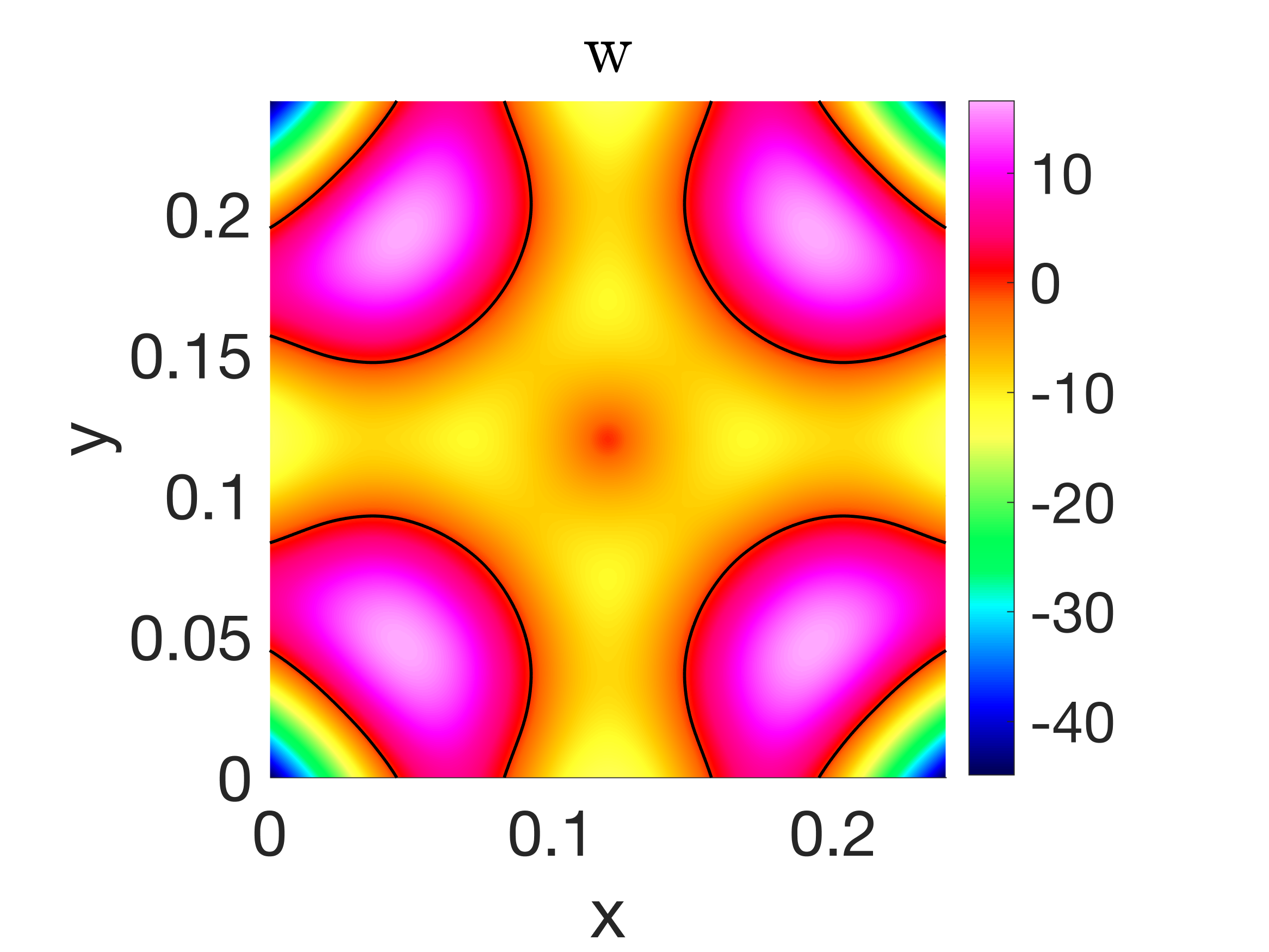
$f_{2}=995.0$Hz

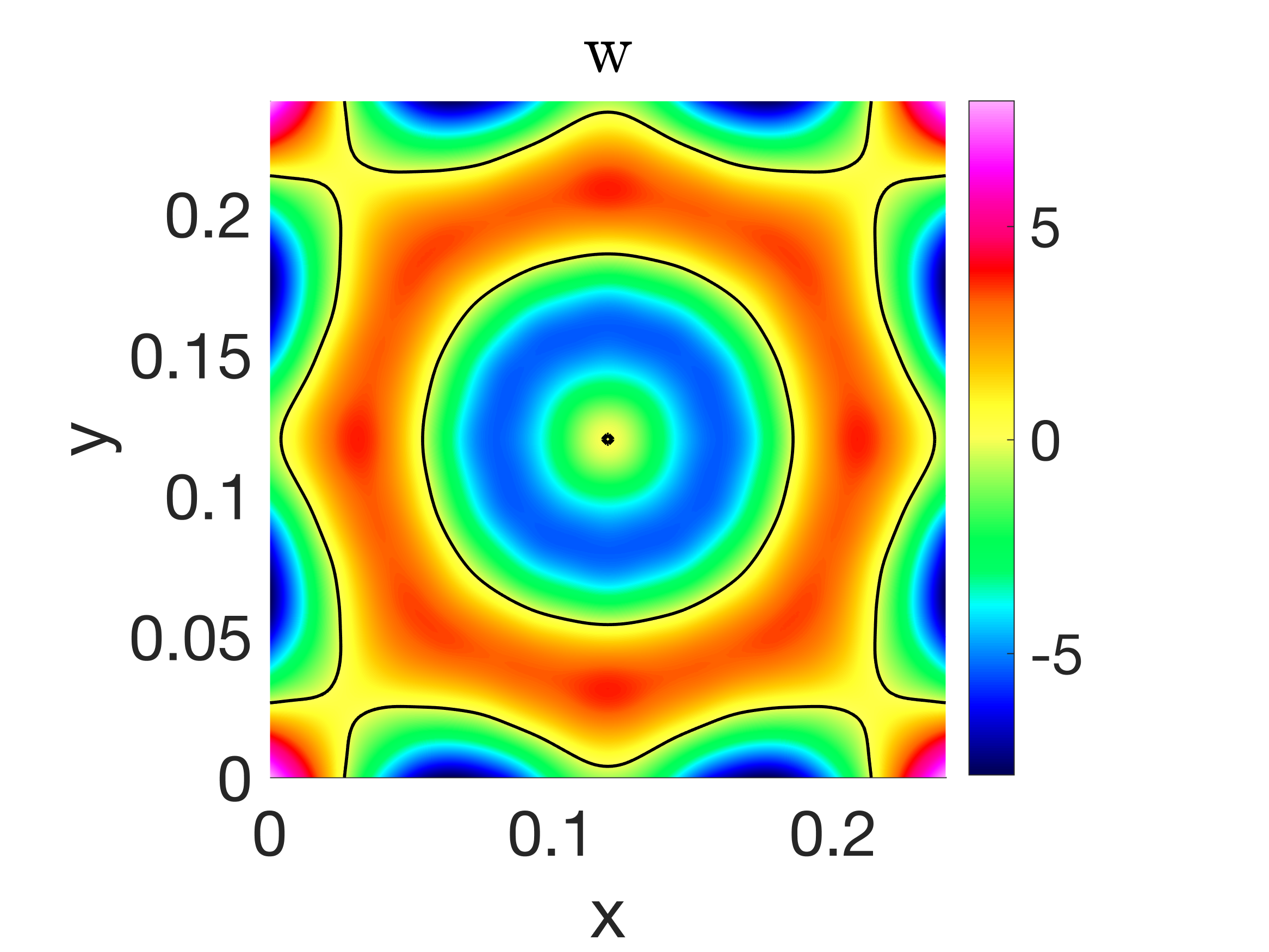
$f_{10}=3443.9$Hz

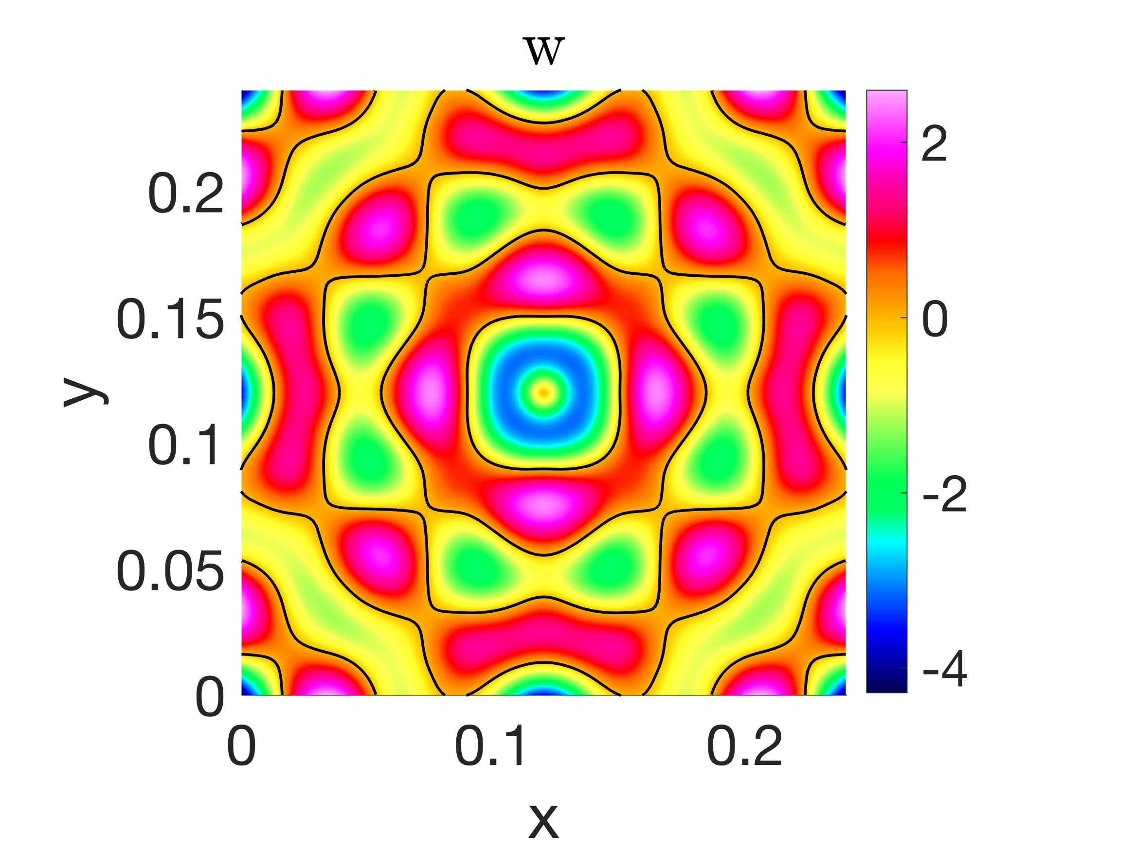
Figure 12: Contour plots of the displacement and the nodal lines (i.e., zero contours) at $t=1$ for three typical resonant frequencies. The results shown here are obtained from the simulation of the NB2 scheme on grid ${\mathcal{G}}_{160}$.

The results obtained from the simulations using the NB2 scheme on grid ${\mathcal{G}}_{160}$ are presented in Figure 12, which includes contour plots of the displacement and the nodal lines at $t=1$ for three typical resonant frequencies. In order to directly compare with the regular frequencies reported in the experiment, we also report in Figure 12 the regular frequencies that are converted from the angular frequencies by $f_{k}={\xi_{k}}/{2\pi}$. The nodal line patterns manifested in our numerical results are in excellent agreement to the experimental results for all the frequencies (except for the degenerate eigenvalues); note that the specific experimental results we are comparing with are reported in Figure 3b in [26].

It is worth pointing out that there are noticeable discrepancies between the values of the numerical and experimental resonant frequencies. This is because the plate model we used for this test is a simple classical Kirchhoff-Love plate that does not consider the influences of the ambient air and the extra mass of the sand particles on the plate. The model could be improved by tuning the various parameters in (1), which is beyond the scope of this study. The purpose of this test is to validate our numerical methods; and the fact that the numerically reconstructed resonant nodal line patterns agree well with the experimental ones and the values of resonant frequencies are in qualitative agreement serves that purpose.

5.3 Application

As an application of our schemes, we numerically explore the interesting physical phenomena known as resonance and beat that occur when the driving frequency is right at or close to a natural frequency. Here we demonstrate the application by considering an annular plate ($\Omega=\{\mathbf{x}:0.1\leq|\mathbf{x}|\leq 0.5\}$) with no external forcing as an example. The plate satisfies the generalized Kirchhoff-Love equation (1) and is driven to vibrate by the following time-dependent clamped boundary conditions that prescribe the displacement of the inner edge; i.e.,

(33) $$w(\mathbf{x},t)=W_{\text{in}}\cos\xi t,\quad\frac{\partial w}{\partial\mathbf{n}}(\mathbf{x},t)=0\leavevmode\nobreak\ \text{for}\leavevmode\nobreak\ |\mathbf{x}|=0.1,$$

where $W_{\text{in}}$ and $\xi$ are the maximum value (amplitude) and angular frequency of the prescribed boundary displacement, respectively. For this example, we set $W_{in}=1$ and vary $\xi$ to investigate its effects. The outer edge of the plate is allowed to move freely; namely, the free boundary conditions (4) are applied at $|\mathbf{x}|=0.5$. Initially, we assume $w_{0}(\mathbf{x},0)=v_{0}(\mathbf{x},0)=0$. The setup of this problem can easily be replicated experimentally by clamping the inner edge of an annular plate to a mechanical oscillator undergoing a sinusoidal motion. The material parameters of the plate are $\rho h=1,D=0.01,T=0,K_{0}=0$, and $\nu=0.3$. With the intention to study the effects of the damping terms in the equation, various values for $K_{1}$ and $T_{1}$ are considered below.

To begin with, we consider the undamped case (i.e., $K_{1}=T_{1}=0$), and specify a value to $\xi$ in (33) that is either close to or at a natural frequency of the plate. Due to the complexity of the generalized plate equation and the time-dependent boundary conditions, it is non-trivial to analytically find the frequency domain eigenvalue problem and then solve it for the natural frequencies and modes as were done in Section 5.2. Following a procedure proposed in [27], we illustrate a more general strategy to identify the natural frequencies of a plate using our numerical methods in conjunction with a fast Fourier transformation (FFT) power spectrum analysis of the numerical data.

The strategy for finding a natural frequency goes as following. We first simulate the problem for an arbitrary driving frequency; say, $\xi=2\pi$ (or $f_{d}=1$ Hz), and trace the response of the plate at $\mathbf{x}_{p}=(-0.2,0)$. The simulation runs until $t=30$ using the NB2 scheme on grid ${\mathcal{G}}_{80}$. The left image of Figure 13 shows the displacement response at the selected location over time. We then perform FFT to the displacement data using the fft function in MATLAB, and present its power spectrum in the right image of Figure 13. From this graph, we are able to identify two natural frequencies ($f_{1}=0.367$, $f_{2}=2.067$) and the driving frequency ($f_{d}=1$). More natural frequencies can be identified this way by sampling different values for the driving frequency $\xi$.

$w(\mathbf{x}_{p},t)$

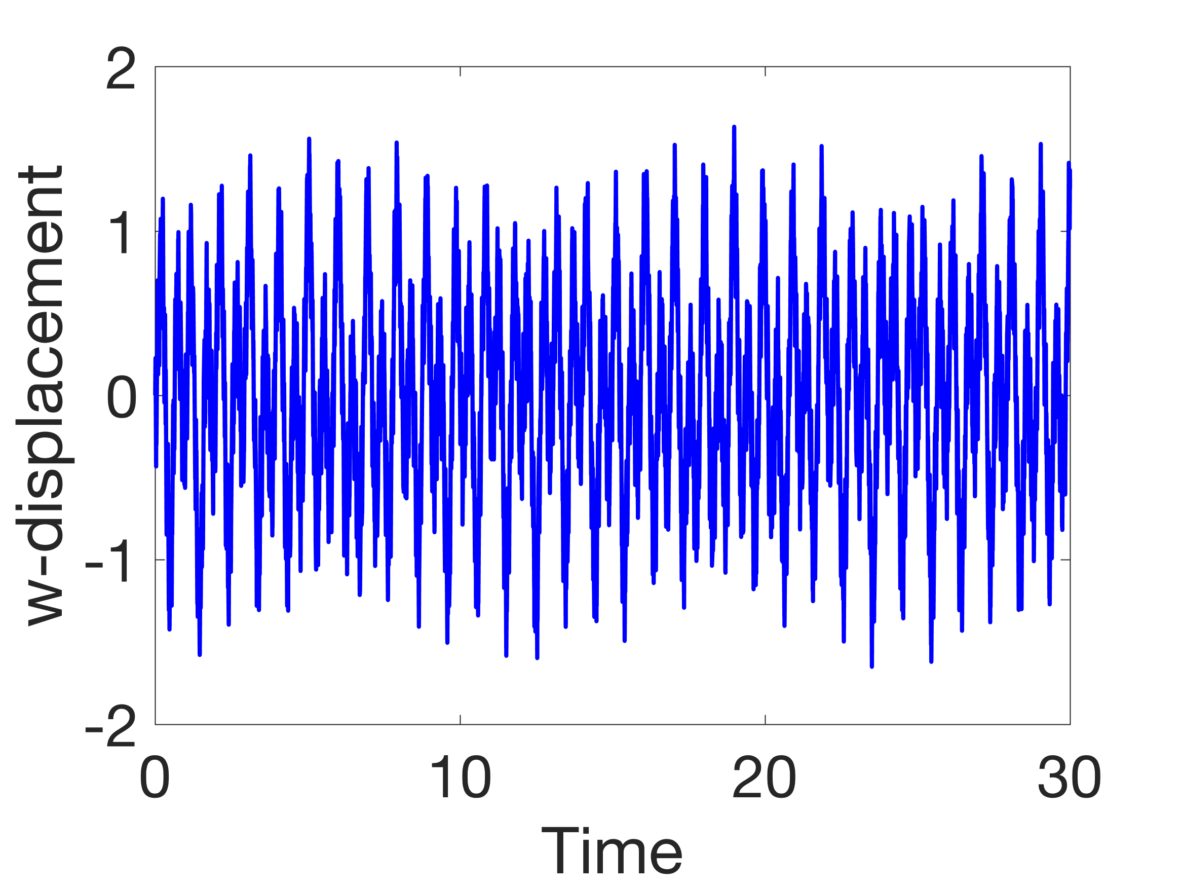
FFT of $w(\mathbf{x}_{p},t)$

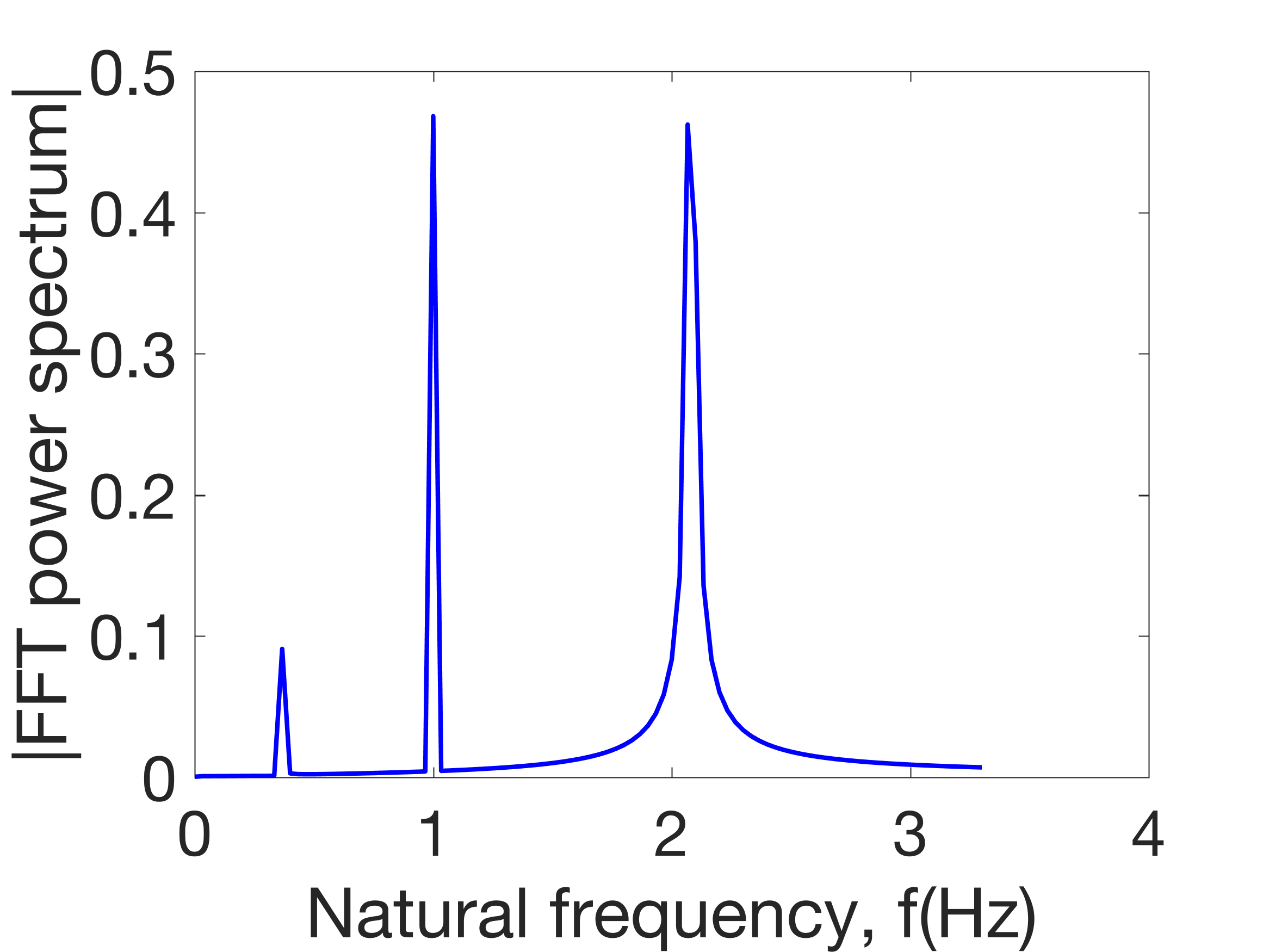
Figure 13: Vibration of the plate when the driving frequency is $\xi=2\pi$ (or $f_{d}=1$ Hz). The simulation runs until $t=30$ using the NB2 scheme on grid ${\mathcal{G}}_{80}$. Left: the displacement response at the selected location $\mathbf{x}_{p}=(-0.2,0)$ over time. Right: the FFT power spectrum of the displacement response.

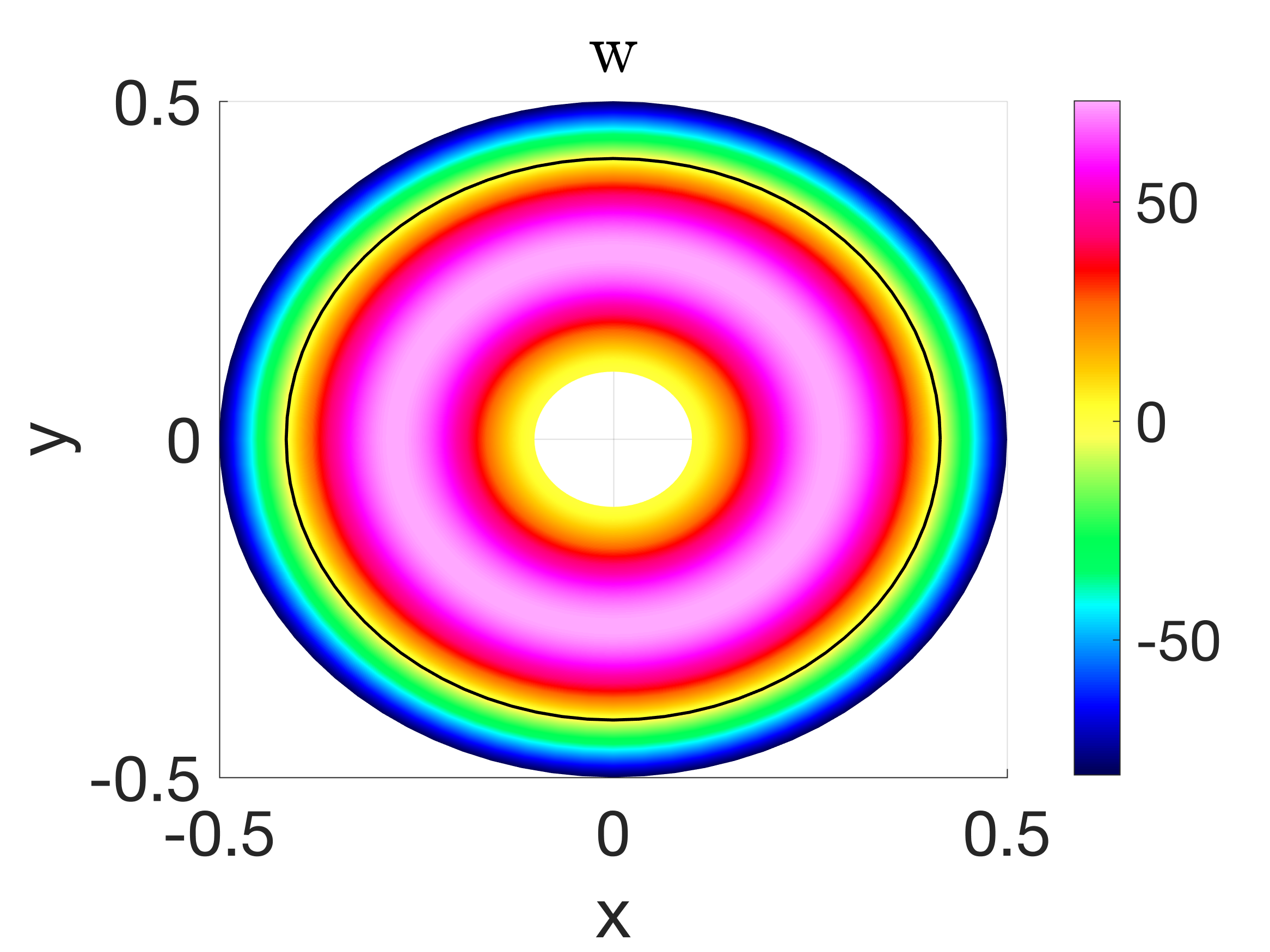
(a) contour of $w(\mathbf{x},30)$

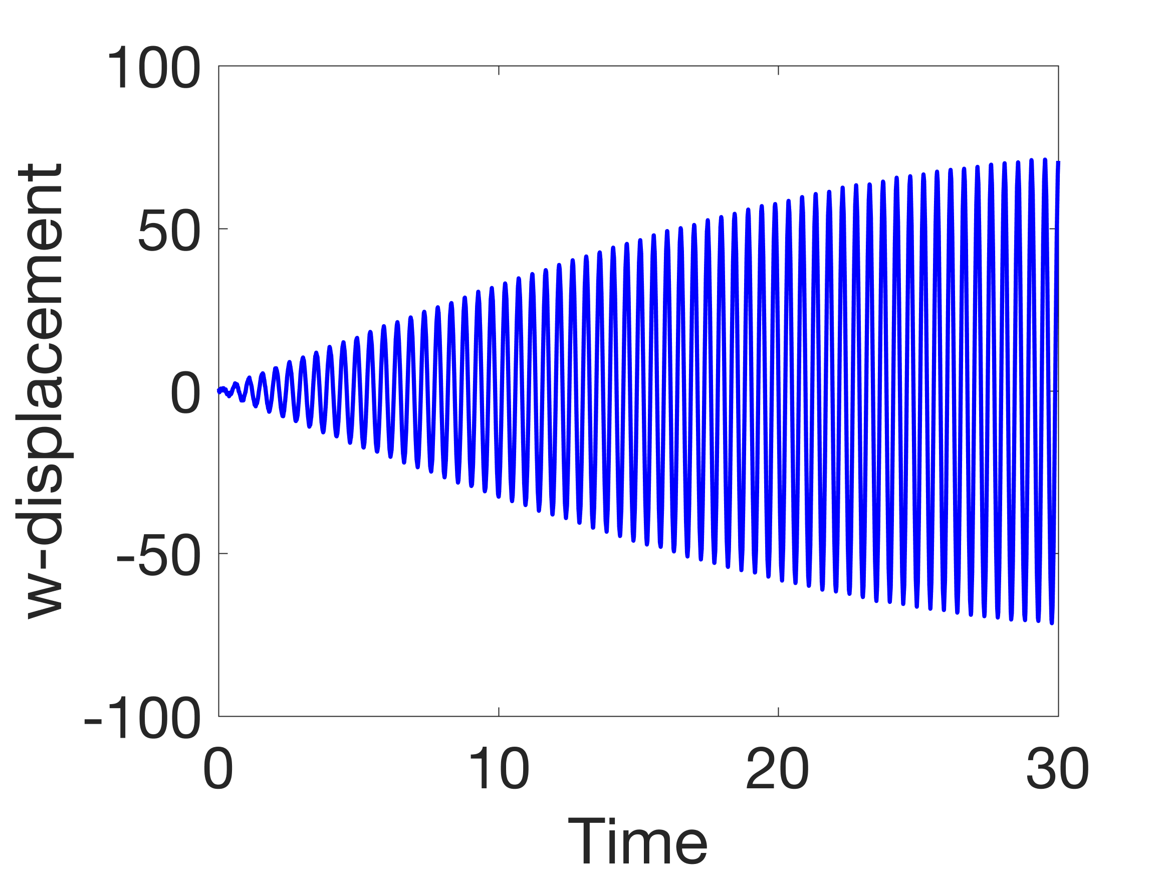
(b) $w(\mathbf{x}_{p},t)$

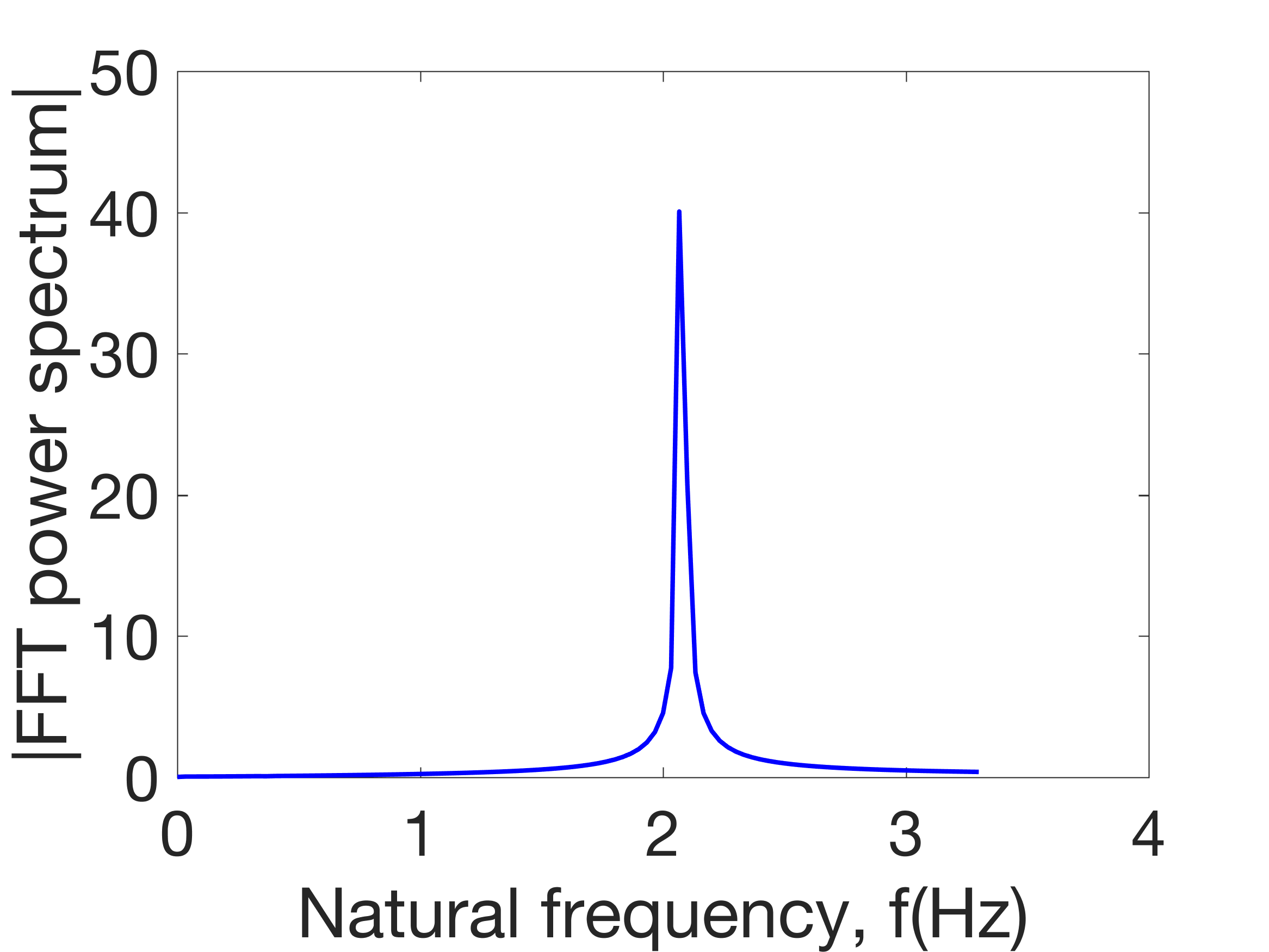
(c) FFT of $w(\mathbf{x}_{p},t)$

Figure 14: Numerical simulation of the resonance phenomenon using the NB2 method on grid ${\mathcal{G}}_{80}$. Here the driving frequency is $\xi_{2}=2\pi f_{2}$ and the probed location is $\mathbf{x}_{p}=(-0.2,0)$.

Resonance occurs when the driving frequency of the plate is at a natural frequency. As an example, we simulate this phenomenon at the natural frequency $f_{2}$ by setting the driving frequency as $\xi_{2}=2\pi f_{2}$. The simulation is carried out using the NB2 scheme until $t=30$, and the results are collected in Figure 14. In particular, we show in Figure 14(a) the contour plot of $w$ as well as its nodal lines at $t=30$. The nodal line pattern sheds light on the mode shape (eigenfunction) associated with the natural frequency $f_{2}$. We also trace the displacement at the point $\mathbf{x}_{p}=(-0.2,0)$ and depict its time history in Figure 14(b). The resonance phenomenon is clearly observed as the amplitude of the vibration increases over time. The FFT power spectrum of the displacement data at this point, as is shown in Figure 14(c), also confirms that the plate vibrates at a frequency consistent with the natural frequency $f_{2}$.

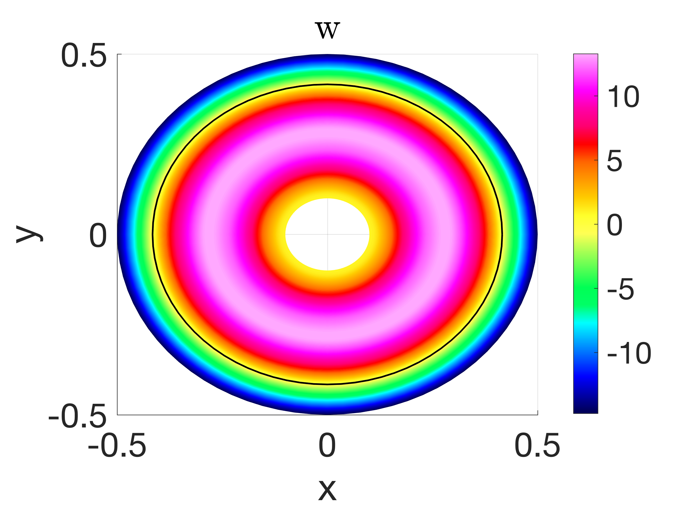
(a) contour of $w(\mathbf{x},30)$

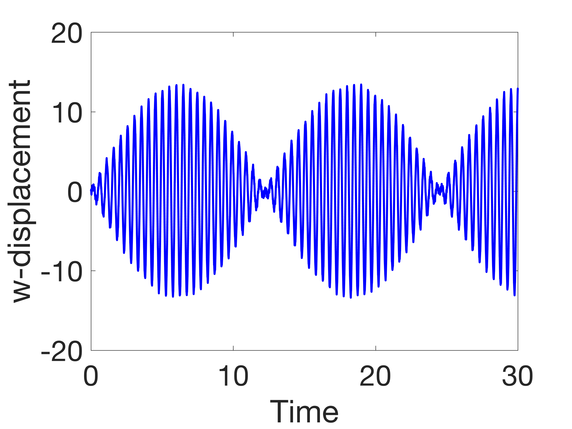
(b) $w(\mathbf{x}_{p},t)$

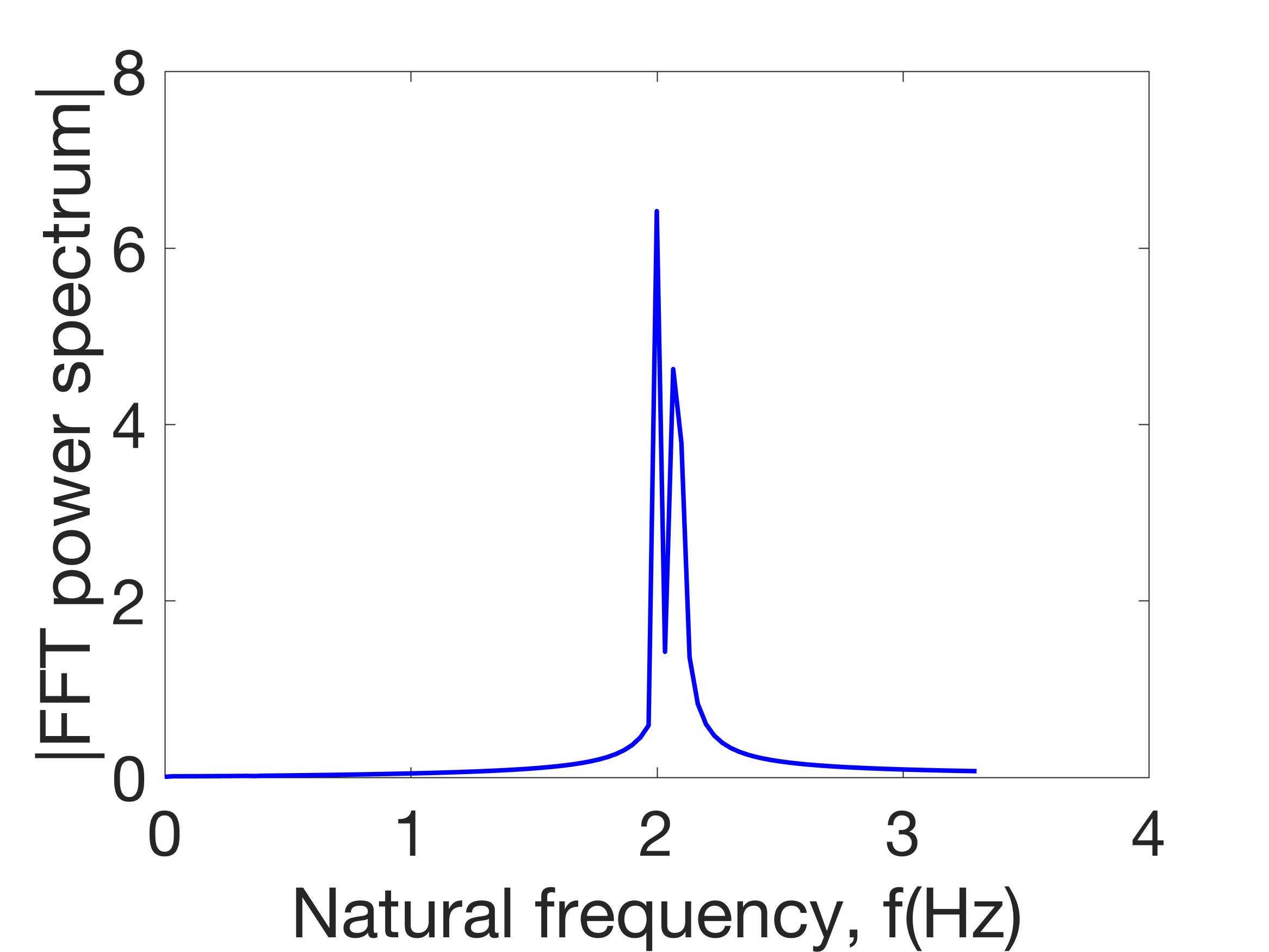
(c) FFT of $w(\mathbf{x}_{p},t)$

Figure 15: Numerical simulation of the beat phenomenon using the NB2 method on grid ${\mathcal{G}}_{80}$. Here the driving frequency is $\xi_{b}=4\pi$ (or $f_{b}=2$ Hz) that is close to the natural frequency $2\pi f_{2}$ and the probed location is $\mathbf{x}_{p}=(-0.2,0)$.

To simulate beat, we drive the plate at a frequency that is very close to the previously found natural frequency $f_{2}$. Therefore, we set the driving frequency in (33) as the so-call beat frequency $\xi_{b}=4\pi$ (or $f_{b}=2$ Hz), noting that the difference between the beat frequency and the natural frequency $f_{2}$ is small for $|f_{b}-f_{2}|=0.067$. Again, the simulation is performed using the NB2 scheme until $t=30$, and a similar collection of results are presented in Figure 15. The nodal line pattern for this case (Figure 15(a)) is in accordance with that shown in Figure 14(a). Furthermore, Figure 15(b) shows the expected oscillation pattern that resembles the beat phenomenon. The FFT power spectrum of the displacement data at $\mathbf{x}_{p}$, as is shown in Figure 15(c), clearly shows the two adjacent frequencies that correspond respectively to the beat frequency $f_{b}$ and the natural frequency $f_{2}$.

Figure 16: Plot of $w(\mathbf{x}_{p},t)$ vs. $t$ for three different damping scenarios. Simulations are carried out using the NB2 scheme on grid ${\mathcal{G}}_{80}$. Here the driving frequency is the same as the resonant frequency $\xi_{2}=2\pi f_{2}$ and $\mathbf{x}_{p}=(-0.2,0)$.

Now, we consider the effects of the damping terms in the generalized Kirchhoff-Love plate (1), which are the linear damping term with coefficient ${K}_{1}$ and the visco-elastic damping term with coefficient ${T}_{1}$. The visco-elastic damping tends to smooth high-frequency oscillations in space and is often added to model vascular structures in haemodynamics. For the simulation, we use the same numerical setup as the resonance example, and demonstrate the damping effects by tracking the displacement over time at the point $\mathbf{x}_{p}=(-0.2,0)$ for three combinations of $K_{1}$ and $T_{1}$ values. The time history of the displacements are shown in Figure 16. For the case when only the linear damping term $(K_{1}=5,{T_{1}=0})$ is added, we can see from the plot that the amplitude of the oscillation is damped down to around $2$ when compared with the undamped resonance case. If we zoom in the plot at early times, we do see some high-frequency oscillations. However, when the visco-elastic damping term is included (${K_{1}=0},T_{1}=0.1$), we can no longer see the high-frequency oscillations in the zoomed in plot; therefore, this term serves to smooth the wave as expected.

Similar numerical results can also be obtained using the PC22 method, although all the simulations are conducted with the NB2 scheme in this section. It is important to remark that the examples considered here also showcase the accuracy and efficiency of our numerical methods. The fact that we are able to simulate the resonance and beat phenomena using a numerically found natural frequency and that the numerically observed resonance frequency further corroborates that value strongly suggests the accuracy of our computations.

6 Conclusions

In this paper, we propose two numerical schemes, referred to as the PC22 and the NB2 schemes, for the approximation of a generalized Kirchhoff-Love plate model. Both schemes are based on centered finite difference methods of second-order accuracy for spatial discretization; and the resulted spatially discretized equations are then advanced in time using an appropriate time-stepping scheme. The PC22 scheme uses an explicit predictor-corrector scheme that consists of a second-order Adams-Bashforth (AB2) predictor and a second-order Adams-Moulton (AM2) corrector, and the NB2 scheme utilizes an implicit Newmark-Beta scheme of second-order accuracy. Stable and accurate numerical boundary conditions are also derived for three common plate boundary conditions (clamped, simply supported and free). Stability analysis is performed for the time-stepping schemes to find the regions of absolute stability, which are utilized to determine stable time steps for both proposed schemes.

Carefully designed test problems are solved to demonstrate the properties and applications of our numerical approaches. The stability and accuracy of the schemes are verified by mesh refinement studies using problems with known exact solutions, and by cross-validation with experimental results. An interesting application concerning the exploration of the resonance and beat phenomena of an annular plate with general configurations is considered to further display the accuracy and efficiency of the numerical methods.

The domains of all the examples considered in this paper are restricted to simple ones that can be discretized with a single Cartesian or curvilinear mesh. We would like to extend the schemes for more general geometries using composite overlapping grids [28]. According to previous studies for wave-like equations on overlapping grids [29], we expect weak instabilities to occur near the interpolation points of the overlapping grids. Therefore, the investigation of novel methods, such as adding high-order spatial dissipation and upwind schemes, to suppress possible instabilities that can be generated from the overlapping grid interpolation would be interesting topics for future research.

Appendix A Nodal line patterns for the eigenvalue problem

We show the results of the eigenvalue problem (31) here. Nodal lines of the first $25$ eigenmodes (with multiplicity) for the square plate with clamped edges and the annular plate with simply supported boundaries are shown in Figures 17 & 18, respectively. The eigenmodes plotted for each degenerated pair are arbitrary so they can be asymmetric.

Figure 17: Nodal lines of the first $25$ eigenmodes (with multiplicity) of the clamped square plate. There are $6$ degenerate pairs of eigenmodes, so that only $19$ distinct normalized eigenvalues are represented. Values reported in the plots are the natural frequencies in increasing order.

Figure 18: Nodal lines of the first $25$ eigenmodes (with multiplicity) of the simply supported annular plate. There are $11$ degenerate pairs of eigenmodes, so that only $14$ distinct eigenvalues are represented. Values reported in the plots are the natural frequencies in increasing order.

References

- [1] E. Reissner, On the theory of transverse bending of elastic plates, Int. J. Solids Struct. 12 (1976) 545 – 554.
- [2] S. Timoshenko, S. Woinowsky-Krieger, Theory of Plates and Shells, 2nd Edition, McGraw-Hill, 1959.
- [3] A. Leissa, Vibration of plates, Tech. Rep. NASA-SP-160, NASA (1969).
- [4] A. E. H. Love, The small free vibrations and deformation of a thin elastic shell, Philos. T. R. Soc. A 179 (1888) 491– 546.
- [5] W. T. Koiter, J. G. Simmonds, Foundations of shell theory, in: E. Becker, G. K. Mikhailov (Eds.), Theoretical and Applied Mechanics, Springer Berlin Heidelberg, Berlin, Heidelberg, 1973, pp. 150 – 176.
- [6] R. D. Mindlin, Influence of rotatory inertia and shear on flexural motions of isotropic, elastic plates, J. Appl. Mech. 18 (1) (1951) 31–38.
- [7] W. T. Koiter, A consistent first approximation in the general theory of thin elastic shells, in: Proceedings of the IUTAM Symposium on the Theory of Thin Elastic Shells, North–Holland, Amsterdam, 1960, pp. 12–33.
- [8] S. Čanić, J. Tambača, G. Guidoboni, A. Mikelić, C. J. Hartley, D. Rosenstrauch, Modeling viscoelastic behavior of arterial walls and their interaction with pulsatile blood flow, SIAM J. Appl. Math. 67 (1) (2006) 164–193.
- [9] J. W. Banks, W. D. Henshaw, D. W. Schwendeman, An analysis of a new stable partitioned algorithm for FSI problems. Part II: Incompressible flow and structural shells, J. Comput. Phys. 268 (2014) 399–416.
- [10] L. Li, W. D. Henshaw, J. W. Banks, D. W. Schwendeman, G. A. Main, A stable partitioned FSI algorithm for incompressible flow and deforming beams, J. Comput. Phys. 312 (2016) 272–306.
- [11] R. Szilard, Theories and Applications of Plate Analysis: Classical Numerical and Engineering Methods, John Wiley & Sons, Ltd, 2004.
- [12] S. Bilbao, A family of conservative finite difference schemes for the dynamical von Karman plate equations, Numer. Methods Partial Differential Equations 24 (1) (2008) 193–216.
- [13] H. Ji, L. Li, Numerical methods for thermally stressed shallow shell equations, J. Comput. Appl. Math. 362 (2019) 626–652.
- [14] J.-L. Batoz, An explicit formulation for an efficient triangular plate-bending element, Int. J. Numer. Meth. Eng. 18 (1982) 1077–1089.
- [15] A. Ibrahimbegović, Quadrilateral finite elements for analysis of thick and thin plates, Comput. Method. Appl. Mech. Engrg. 110 (1993) 195–209.
- [16] E. Oñate, F. Zárate, Rotation-free triangular plate and shell elements, Int. J. Numer. Meth. Eng. 47 (2000) 557–603.
- [17] L. B. da Veiga, J. Niiranen, R. Stenberg, A family of finite elements for Kirchhoff plates I: Error analysis, SIAM J. Numer. Anal. 45 (2007) 2047–2071.
- [18] M. Bischoff, K.-U. Bletzinger, W. Wall, E. Ramm, Models and Finite Elements for Thin-Walled Structures, Vol. 2, 2004.
- [19] L. B. da Veiga, J. Niiranen, R. Stenberg, A new finite element method for kirchhoff plates, in: C. A. Motasoares, J. A. C. Martins, H. C. Rodrigues, J. A. C. Ambrósio, C. A. B. Pina, C. M. Motasoares, E. B. R. Pereira, J. Folgado (Eds.), III European Conference on Computational Mechanics, Springer Netherlands, Dordrecht, 2006, pp. 51–51.
- [20] L. Perotti, A. Bompadre, M. Ortiz, Automatically inf-sup compliant diamond-mixed finite elements for Kirchhoff plates, Int. J. Numer. Meth. Eng. 96 (2013) 405–424.
- [21] J. Huang, X. Huang, Y. Xu, Convergence of an adaptive mixed finite element method for Kirchhoff plate bending problems, SIAM J. Numer. Anal. 49 (2011) 574–607.
- [22] E. Bécache, G. Derveaux, P. Joly, An efficient numerical method for the resolution of the Kirchhoff-Love dynamic plate equation, Numer. Methods Partial Differential Equations 21 (2) (2005) 323–348.
- [23] A. Frangi, M. Guiggiani, Boundary element analysis of Kirchhoff plates with direct evaluation of hypersingular integrals, Int. J. Numer. Meth. Eng.
- [24] D. Benson, Y. Bazilevs, M. Hsu, T. Hughes, Isogeometric shell analysis: The Reissner-Mindlin shell, Comput. Method. Appl. Mech. Engrg. 199 (5) (2010) 276 – 289, computational Geometry and Analysis.
- [25] N. M. Newmark, A method of computation for structrual dynamics, proceedings of the american society of civil engineers 85 (EM 3) (1959) 67–74.
- [26] P. H. Tuan, C. P. Wen, P. Y. Chiang, Y. T. Yu, H. C. Liang, K. F. Huang, Y. F. Chen, Exploring the resonant vibration of thin plates: Reconstruction of chladni patterns and determination of resonant wave numbers, J. Acoust. Soc. Am. 137 (2015) 2113–2123.
- [27] A. Chugh, Natural vibration characteristics of gravity structures, Int. J. Numer. Anal. Meth. Geomech. 31 (2007) 607 – 648.
- [28] G. S. Chesshire, W. D. Henshaw, Composite overlapping meshes for the solution of partial differential equations, J. Comput. Phys. 90 (1) (1990) 1–64.
- [29] W. D. Henshaw, A high-order accurate parallel solver for Maxwell’s equations on overlapping grids, SIAM J. Sci. Comput. 28 (5) (2006) 1730–1765.