Dispersionless pulse transport in mass-spring chains:
All possible perfect Newton’s cradles

Abstract

A pulse traveling on a uniform nondissipative chain of $N$ masses connected by springs is soon destructured by dispersion. Here it is shown that a proper modulation of the masses and the elastic constants makes it possible to obtain a periodic dynamics and a perfect transmission of any kind of pulse between the chain ends, since the initial configuration evolves to its mirror image in the half period. This makes the chain to behave as a Newton’s cradle. By a known algorithm based on orthogonal polynomials one can numerically solve the general inverse problem leading from the spectrum to the dynamical matrix and then to the corresponding mass-spring sequence, so yielding all possible “perfect cradles”. As quantum linear systems obey the same dynamics of their classical counterparts, these results also apply to the quantum case: for instance, a wavefunction localized at one end would evolve to its mirror image at the opposite chain end.

I Introduction

By mass-spring chain one means a sequence of $N$ masses $\{m_{i}\}$ connected by $N{-}1$ springs obeying Hooke’s law and characterized by their elastic constants $\{K_{i}\}$. The system’s Hamiltonian reads

$${\cal{H}}=\sum_{i=1}^{N}\frac{P_{i}^{2}}{2m_{i}}+\frac{1}{2}\sum_{i=1}^{N-1}K_{i}(Q_{i}-Q_{i{+}1})^{2}~{},$$ (1)

where $Q_{i}$ is the displacement (measured from the equilibrium position) and $P_{i}$ the momentum of the $i$-th mass. This physical model, depicted in Fig. 1, is very general: for instance, it can be realized by the electric LC circuit of Fig. 2, where springs and masses are replaced by capacitors and inductors, respectively, while displacements are represented by the capacitors’ charges.

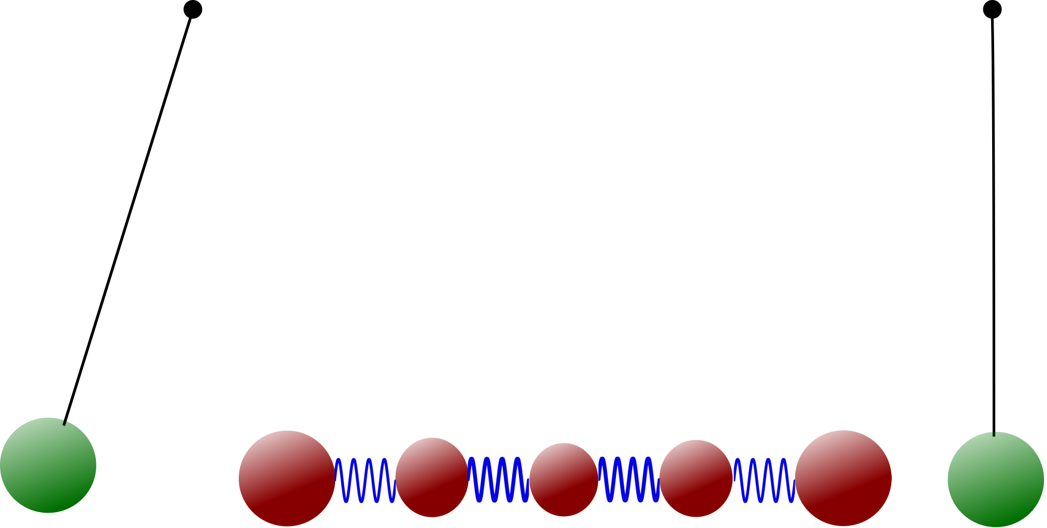
Figure 1: A perfect 5-mass chain. The masses are proportional to the sequence (35, 20, 18, 20, 35) and the springs’ elastic constants to $(7,9,9,7)$: this setup yields perfect end-to-end transmission HerrmannS1981 . The auxiliary (green) external masses, equal to the first/last ones, behave just like in a Newton’s cradle, except for the finite time between subsequent bounces. Chains of arbitrary length can behave in the same way, provided that the sequence of mass and spring values be properly chosen.

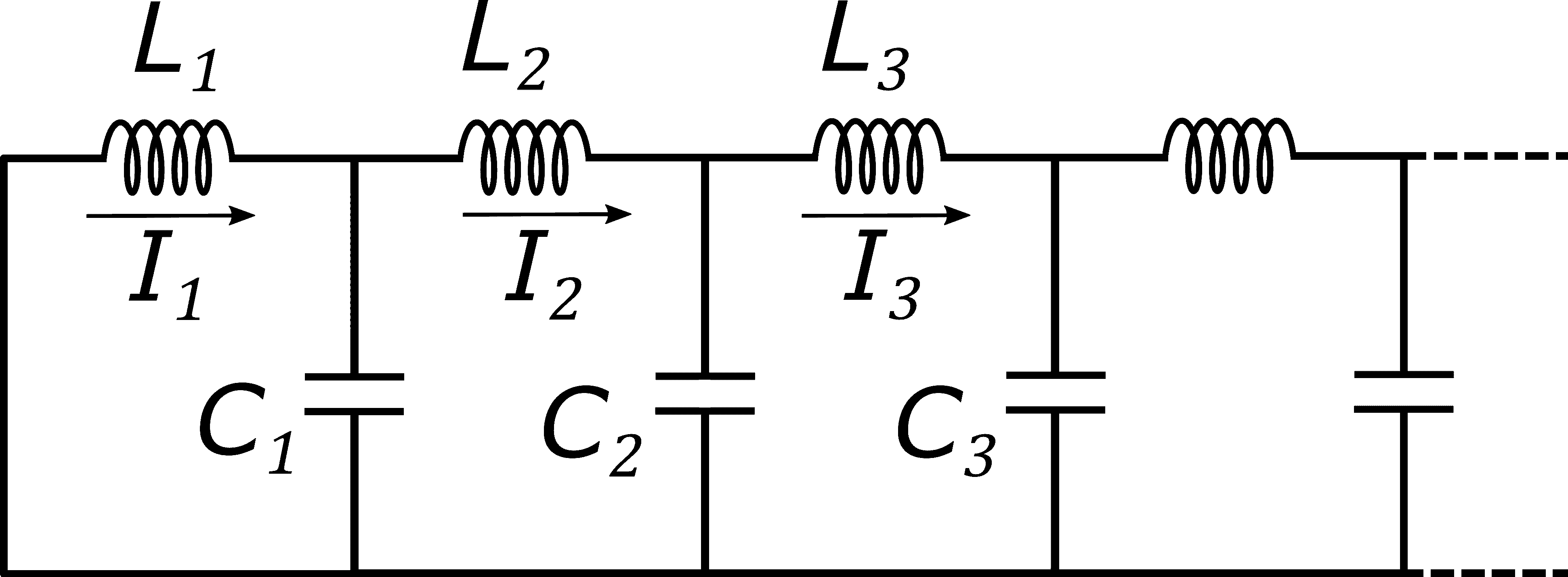
Figure 2: An electric circuit equivalent to the spring-mass chain (1): the masses and the elastic constants are replaced by the inductances and inverse capacitances, respectively: $m_{i}=L_{i}$ and $K_{i}={C^{-1}_{i}}$. The charges $Q_{i}$ flowing in the conductances ($\partial_{t}{Q}_{i}=I_{i}$) play the role of the displacements and the momenta are $P_{i}=L_{i}I_{i}$. The charge on capacitor $C_{i}$ is $Q_{i}-Q_{i+1}$.

Nanoscopic realizations of the model (1) are relevant for their end-to-end transport properties CahillEtAl2003 ; NorrisLB2013 and even atomic chains, which can be suitably described by the mass-spring chain model, have been created and characterized RammPH2014 , e.g., studying the transmission of a momentum pulse given to an extremal atom.

The purpose of this paper is to demonstrate the existence, for any chain length $N$, of an infinite number of sequences $\{m_{i}\}$ and $\{K_{i}\}$ which can yield the perfect end-to-end transmission of such a pulse. For this reason such mass-spring chains behave in analogy to the popular Newton’s cradle HerrmannS1982 ; HutzlerDWM2004 , a mechanical device that displays an almost perfect transfer of momentum between the endpoints of an array of metallic spheres. Dubbing them “mass-spring Newton’s cradles” is therefore natural, also looking at Fig. 1, and justified by the wide use of this terminology in physical systems where one can observe the perfect transfer of a localized conserved quantity over a one-dimensional structure, e.g., the “quantum Newton’s cradle” of Ref. KinoshitaWW2006 .

It is well known that a uniform mass-spring chain, made of identical masses $m_{i}=m$ and identical springs $K_{i}=K$, cannot efficiently transfer a pulse, even in the absence of dissipation, due to the effect of dispersion. Indeed, its normal modes, which coincide with the Fourier components of the coordinates and momenta, do have incommensurate frequencies Kittel1953 ,

$$\omega_{n}=2\sqrt{\frac{K}{m}}\,\sin\frac{\pi(n-1)}{2N},,~{}~{}~{}~{}n=1,...,N~{},$$ (2)

$n$ being the normal-mode label. It follows that their time evolution, ruled by the phase factors $e^{-i\omega_{n}t}$, can never lead to coherently recombining their amplitudes, i.e., with equal phases.

It is worth to mention that, historically, the research for coherent transmission of signals along one-dimensional systems preferred to renounce to the linearity (i.e., using non-Hooke springs), while keeping translation invariance, i.e., uniformity. Starting from the famous Fermi-Pasta-Ulam numerical simulation FermiPU1955 , more and more studies enlightened the properties of nonlinear models and showed that nonlinearity can be an antidote against dispersion; several examples of localized and coherently propagating excitations, the “solitons”, were discovered, such as in the Toda lattice, or in the continuous systems described by the Korteweg-De Vries equation (known since the 19th century) and the Nonlinear Schrödinger equation, just to mention the most well-known ones DauxoisP2006 .

At variance with this way to reach coherence, in this paper Hooke’s law is kept and translation invariance is instead abandoned, so dealing with nonuniform chains. Conceding a limited degree of nonuniformity, it was possible Vaia2018 to enhance the transmission properties of the linear chain (1) keeping it uniform in the bulk and symmetrically tuning two masses and their spring at both ends, in order to maximize the transmission of a pulse given to the first mass. Such a tuning has two main effects, namely, modulation of the amplitudes of the excited normal modes and deformation of the frequency spectrum: the best trade-off between them produces a huge improvement in the end-to-end transmission efficiency, attaining 98.7 % in the asymptotic limit of infinite length Vaia2018 . The explanation is that only few normal modes with nearly equally-spaced frequencies are involved in the dynamics of the initial kick. However, this approach is very particular: it yields optimal, but not perfect, transmission and only for excitations localized on the first mass; a kick given, say, to the second mass would not coherently reach the opposite end.

Allowing for full nonuniformity, here a different questions are raised: Can one obtain “magic” mass-spring sequences that yield an exactly periodic and perfectly transmitting dynamics? How many of those sequences exist?

An obvious requirement for coherence is that the normal-mode frequencies be commensurate, i.e., integer multiples of a finite frequency $\omega$, say

$$\omega_{n}=\omega\,{k_{n}},$$ (3)

with $\{k_{n}\}$ any sequence of integers (with no common factors, to be absorbed into $\omega$). Indeed, the dynamical phases, evolving as $e^{i\omega\,k_{n}t}$, would become unity after a time period $2\pi/\omega$ (and integer multiples of it); then, the normal modes would coherently recombine to exactly reproduce the initial configuration. It is again obvious that, in order to yield the spectrum (3), one must renounce the assumption of uniform masses and springs along the chain, as they give (2). However, in order to be effective for transmission, the chain must allow for pulses traveling from one extremity to reproduce themselves at the opposite one without changes in shape: this entails that the chain has to be at least mirror symmetric, i.e., the transformation of inverting the sequence of masses and springs is a symmetry,

$$m_{i}=m_{N{+}1-i}~{},~{}~{}~{}~{}~{}K_{i}=K_{N-i}~{};$$ (4)

the $2N\,{-}\,1$ parameters $\{m_{i},K_{i}\}$ are therefore reduced to $N$ independent ones. With this assumption, it will be shown that if the above defined integers $\{k_{n}\}$ are alternating in parity, then at the half period $t^{*}=\pi/\omega$ (and odd multiples of it) the chain configuration becomes the mirror image of the initial one, so that any pulse at one end would be transferred to the opposite end with identical shape. It will be also proven that the “magic” mass-spring sequences exist and are in one-to-one correspondence with the distinct successions of the $N$ integers $\{k_{n}\}$ defined in Eq. (3), attaining the goal of finding and classifying all perfect chains, i.e., those with full 100 % transmission efficiency whatever the shape of the initial pulse.

As for the mathematical methods, the task of finding the normal modes and the frequencies of the mass-spring chain (1) can be reduced, by using mass-weighted canonical variables, to the diagonalization of a tridiagonal symmetric matrix, usually dubbed a Jacobi matrix Parlett1998 . The chain’s mirror symmetry further entails it to be symmetric also with respect to the second diagonal, so one deals with a persymmetric Jacobi matrix. The goal pursued here is however the inverse problem, namely one starts from the desired eigenvalue succession (3) and wishes to obtain the corresponding Jacobi matrix and, in turn, the related mass-spring sequence. Fortunately, it is known that the inverse problem of calculating the elements of a persymmetric Jacobi matrix, such that its eigenvalues be a given nondegenerate note1 sequence, is well-posed and the solution has been proven to exist Hochstadt1967 and to be unique Hald1976 . Moreover, the matrix elements can be calculated, at least numerically, by means of efficient algorithms deBoorG1978 . The remaining task of relating these elements to the values of the masses and of the spring constants, can also be unambiguously solved NylenU1997 .

Remarkably, an explicit analytic solution to the inverse problem was recently found VaiaS2020 for any $N$ when $k_{n}=n-1$, i.e., the frequencies are proportional to the sequence of the first $N$ integers,

$$\omega_{n}=\omega\,(n{-}1),~{}~{}~{}~{}n=1,...,N~{}.$$ (5)

For instance, with $N=5$ one gets the chain of Fig. 1. For $N\leq 5$ the exact solution was already known HerrmannS1981 , though the calculations were not published, being “somewhat lengthy”. On the other hand, for arbitrary sequences of integers in Eq. (3) a numerical approach cannot be avoided. It will be shown that a variety of perfect chains can be obtained, with some of them even more interesting as they entail smaller imbalances between largest and smallest masses and elastic constants. All these “perfect chains” can be employed in different contexts for transmitting localized pulses (say, energy, heat, sound, etc.) between their extrema; perhaps such a mechanism might be already used by Nature, e.g., for transferring energy inside biological structures. It is to be emphasized that, since the model system is linear, the corresponding quantum model also shows an analogous behavior; for instance, the quantum wave function of such an array evolves in the time $t^{*}$ to its mirror-symmetric counterpart, which amounts to state that a localized wavepacket at one end would be perfectly transmitted to the opposite end of the chain.

The paper is organized as follows. Basic notations and definitions are briefly recalled in Section II, as well as the dynamics of the chain in terms of its normal modes. In Section III the transmission amplitude is defined as indicator of the pulse-transfer efficiency. The inverse problem and the solution algorithm are the subject of Section IV. Eventually, in Section V the dynamics of different mass-spring chains are compared and discussed, including the uniform, the optimized quasi-uniform Vaia2018 , and the perfect chains with the spectrum (5) and more selected perfect chains.

II The free mass-spring chain

Consider the chain described by the Hamiltonian (1); the absence of external springs (free-free boundary conditions, i.e., $K_{0}=K_{N}=0$) entails translation invariance, so that the system is expected to possess a zero-frequency normal mode (translation mode). In terms of the displacement and momentum vectors, ${\bm{Q}}\equiv\{Q_{i}\}$ and ${\bm{P}}\equiv\{P_{i}\}$, the same Hamiltonian can be written in matrix form,

$${\cal{H}}=\frac{1}{2}\,{\bm{P}}^{\rm T}\bm{M}^{-1}{\bm{P}}+\frac{1}{2}\,{\bm{Q}}^{\rm T}{\bm{K}}{\bm{Q}}~{},$$ (6)

where the “mass matrix” $\bm{M}$ is diagonal, its elements being $\{M_{ij}=m_{i}\,\delta_{ij}\}$, and

$$\bm{K}=\begin{bmatrix}K_{1}&-K_{1}&0&\cdots\\[5.69054pt] -K_{1}&K_{1}{+}K_{2}&-K_{2}&\cdots\\[5.69054pt] 0&-K_{2}&K_{2}{+}K_{3}&\\[5.69054pt] \vdots&\vdots&&\ddots\end{bmatrix}_{N}~{},$$ (7)

is the symmetric tridiagonal “elastic matrix”. Its rows sum up to zero, so that $\bm{K}$ has the eigenvector $(1,~{}1,~{}...,~{}1)$ corresponding to the translation mode with eigenvalue zero, so ${\rm{det}}\,{\bm{K}}=0$. The canonical transformation to mass-weighted coordinates, ${\bm{q}}={\bm{M}}^{1/2}{\bm{Q}}$ and ${\bm{p}}={\bm{M}}^{-1/2}{\bm{P}}$, turns the Hamiltonian into

$${\cal{H}}=\frac{1}{2}\,{\bm{p}}^{\rm T}{\bm{p}}+\frac{1}{2}\,{\bm{q}}^{\rm T}{\bm{A}}{\bm{q}}~{}.$$ (8)

The $N{\times}N$ matrix ${\bm{A}}={\bm{M}}^{-1/2}{\bm{K}}{\bm{M}}^{-1/2}$ is a Jacobi matrix, i.e., a tridiagonal symmetric matrix,

$$\bm{A}=\begin{bmatrix}a_{1}&-b_{1}&0&\cdots&0\\ -b_{1}&a_{2}&-b_{2}&&\vdots\\ 0&-b_{2}&a_{3}&\ddots&0\\ \vdots&&\ddots&\ddots&-b_{N-1}\\ 0&\cdots&0&-b_{N-1}&a_{N}\end{bmatrix}_{N}~{},$$ (9)

whose nonzero elements are

$$\begin{aligned} a_{i}&=\frac{K_{i-1}+K_{i}}{m_{i}}~{},&~{}~{}~{}&i=1,...,N~{},\\ b_{i}&=\frac{K_{i}}{\sqrt{m_{i}m_{i{+}1}}}~{},&&i=1,\,...,\,N{-}1~{}.\end{aligned}$$ (10)

The assumption of mirror symmetry (4) entails that the matrices ${\bm{M}}$ and ${\bm{K}}$ are persymmetric (symmetric with respect to the antidiagonal), and the same holds for ${\bm{A}}$,

$$a_{i}=a_{N{+}1-i}~{},~{}~{}~{}b_{i}=b_{N-i}~{}.$$ (11)

Note that as ${\rm{det}}\,{\bm{A}}=0$ only $N{-}1$ of these matrix elements are independent. They are in correspondence with the $N$ independent parameters $\{m_{i},K_{i}\}$, apart from an overall factor: indeed, Eq. (10) shows that such a factor does not affect $\bm{A}$, reflecting the fact that scaling masses and spring constants by the same factor does not affect the system’s frequencies and normal modes. This choice is arbitrary, e.g., one can fix the first mass $m_{1}$ or the total mass GantmacherK1950 , and fully completes the mapping between $\bm{A}$ and the pair $(\bm{M},\bm{K})$

As all $b$’s are nonzero the eigenvalues of the matrix $\bm{A}$ are distinct Parlett1998 ; moreover, they are nonnegative since $\bm{A}$ is positive semi-definite,

$$\sum_{ij}A_{ij}q_{i}q_{j}=\sum_{i}K_{i}(Q_{i}-Q_{i+1})^{2}\geq 0~{},~{}~{}~{}~{}\forall\{q_{i}\}~{}.$$ (12)

Denoting by $\bm{U}\,{=}\,\{U_{ni}\}$ the orthogonal matrix that diagonalizes $\bm{A}$,

$$\sum_{ij}U_{ni}A_{ij}U_{mj}=\lambda_{n}\,\delta_{nm}~{},$$ (13)

and introducing the normal-mode coordinates and momenta,

$$\tilde{q}_{n}=\sum_{i=1}^{N}U_{ni}\,q_{i}~{},~{}~{}~{}\tilde{p}_{n}=\sum_{i=1}^{N}U_{ni}\,p_{i}~{},$$ (14)

the Hamiltonian (8) becomes a sum of independent oscillators,

$${\cal{H}}=\frac{1}{2}\sum_{n=1}^{N}\big{(}\tilde{p}_{n}^{2}+\omega_{n}^{2}\,\tilde{q}_{n}^{2}\big{)}~{}.$$ (15)

where the eigenfrequencies are the positive square roots of the eigenvalues, $\omega_{n}=\sqrt{\lambda_{n}}$. They are assumed in increasing order, $\omega_{n+1}>\omega_{n}$, starting from $\omega_{1}=0$.

The chain’s time evolution is a superposition of normal-mode motions,

$$q_{i}(t)=\sum_{n=1}^{N}U_{ni}\sum_{j=1}^{N}U_{nj}\,\Big{[}q_{j}(0)\cos\omega_{n}t+{p_{j}(0)}\frac{\sin\omega_{n}t}{\omega_{n}}\Big{]}~{}.$$ (16)

All frequencies are positive, except that of the translation mode, $\omega_{1}=0$: its corresponding component is to be understood as the overall translation $U_{1i}\sum_{j}U_{1j}\big{[}q_{j}(0)+p_{j}(0)\,t\big{]}$.

III Perfect pulse transmission

The transmission of a pulse between the chain ends can be described as follows. Assume the first mass is given an instantaneous kick, i.e., a given momentum $\bar{p}$, as in experiments with ion chains RammPH2014 ,

$$\bm{q}(0)=(0,\,0,\,...,\,0)~{},~{}~{}~{}~{}\bm{p}(0)=(\bar{p},\,0,\,...,\,0)~{}.$$ (17)

One seeks for values of the chain parameters (4) such that the dynamics leads in a certain time $\tau$ as close as possible to the mirror-symmetric momentum distribution $\bm{p}(\tau)=(0,\,0,\,0,\,...,\,\bar{p})$. With these initial conditions Eq. (16) gives

$$p_{i}(t)=\partial_{t}q_{i}(t)=\bar{p}\sum_{n=1}^{N}U_{ni}U_{n1}\cos\omega_{n}t~{}.$$ (18)

The transmission amplitude $\alpha_{{}_{N}}(t)\equiv{p_{{}_{N}}(t)}/{\bar{p}}$ is defined as the ratio between the momentum of the last mass at time $t$ and the input momentum of the first mass. Using the fact that the eigenvectors of $\bm{A}$ alternate between mirror-symmetric and -antisymmetric CantoniB1976 ; Parlett1998 , $U_{n,N+1-i}\,{=}\,(-)^{n-1}U_{ni}$, one has

$$\alpha_{{}_{N}}(t)=\sum_{n=1}^{N}U_{n1}^{2}\cos[\pi(n{-}1){-}\omega_{n}t]~{}.$$ (19)

The numbers $U_{n1}^{2}$ weigh the contributions from the normal modes and can be regarded as a normalized probability density, since $\sum_{n}U_{n1}^{2}\,{=}\,1$. The same parameter $\alpha_{{}_{N}}(t)$ characterizes the transmission of an initial elongation of the first mass, ${\bm{q}}(0)=(\bar{q},\,0,\,...,\,0)$, while the chain is at rest, $\bm{p}(0)=\bm{0}$: indeed, Eq. (16) yields $q_{{}_{N}}(t)=\bar{q}\,\alpha_{{}_{N}}(t)$.

Perfect transmission occurs when at some time instant $t^{*}$ all phases are coherent, i.e., they are equal or differ by integer multiples of $2\pi$:

$$\pi(n{-}1)-\omega_{n}t^{*}=\pi\times~{}{\rm even~{}integer}~{}.$$ (20)

This amounts to require that the frequencies are integer multiples of a characteristic frequency $\omega=\pi/t^{*}$,

$$\omega_{n}=\omega\,k_{n}~{},$$ (21)

with the (different) coprime integers $k_{n}$ having the same parity of $n{-}1$, since $k_{1}=0$; it is equivalent to require that the increments

$$\delta_{n}\equiv k_{n+1}-k_{n}~{},~{}~{}~{}i=1,\,...,\,N{-}1~{},$$ (22)

be odd positive integers with no common factors (i.e., coprime). In the next section it is shown that that any given frequency spectrum corresponds to a particular mass-spring sequence, so it follows that for any $N\geq 3$ there is a countably infinite set of different chains yielding perfect transmission.

At time $2t^{*}$ the chain returns to the initial state, as, e.g., $p_{1}(2t^{*})=\bar{p}\sum_{n=1}^{N}U_{n1}^{2}\cos(2\pi\,k_{n})=\bar{p}$, showing a perfectly periodic dynamics note2 . The time evolution consists in the propagation of the initial pulse along the chain, with a shape involving displacements of all masses. Actually, perfect behavior does not require the particular initial configuration (17): Eq. (16) with the spectrum (21)-(22) tells that any initial shape of the chain evolves to its exact mirror image at $t^{*}$ and is restored at $2t^{*}$. Such a perfect mass-spring cradle is depicted in Fig. 1: to make it resemble a Newton’s cradle, it is imagined to involve two auxiliary hanging masses that periodically transmit/receive momentum by instantaneous hard-sphere collision with the chain extrema.

The upcoming sections are devoted to the calculation of the “magic” mass-spring sequences that determine $\alpha_{N}(t^{*})=1$, i.e., 100 % transmission amplitude for any value of $N$.

IV The inverse problem

The task of finding the matrix elements of the tridiagonal symmetric and mirror-symmetric matrix (9) starting from the requirement that it have a given spectrum $\{\lambda_{n},~{}n=1,\,...,\,N\}$ is an “inverse problem”. It is well-posed, as in the case considered here (free-free boundary conditions) the number of independent matrix elements to be determined, $N{-}1$, is equal to the number of input variables, the positive eigenvalues.

In the previous Section it was shown that the necessary and sufficient condition to yield perfect transmission is that the mode frequencies be given by Eq. (21), where the increasing sequence of integers $\{k_{n}\}$ obeys the constraint (22).

IV.1 Simplest case: analytic solution

The simplest choice for the odd-number sequence (22) is $\delta_{n}=1$, or $k_{n}=n\,{-}\,1$, corresponding to the spectrum (5). In this case an analytic solution was recently obtained VaiaS2020 , based on the following result, whose proof is sketched in Appendix A. Let $\bm{A}$ be the $N{\times}N$ matrix (9) with the mirror-symmetric entries

$$a_{i} =N{-}1+4(i{-}1)(N{-}i)~{}, i=1,\,...,\,N~{},$$ (23)

$$b_{i} =\sqrt{i\,(2i{-}1)\,(N{-}i)\,(2N{-}1{-}2i)}~{}, i=1,\,...,\,N{-}1~{};$$

then its eigenvalues are

$$\lambda_{n}=2(n{-}1)^{2}~{},~{}~{}~{}~{}~{}~{}n=1,\,...,\,N~{}.$$ (24)

Both $a_{i}$ and $b_{i}$ are of order $N^{2}$ in the matrix bulk, and decrease almost parabolically toward the matrix edges, where they are of order $N$. Their imbalance, namely the ratio between largest and smallest entries, is of order $N$.

Hence, the frequency sequence $\omega_{n}=\omega\,(n\,{-}\,1)$ can be obtained by imposing a factor $\omega^{2}/2$ to the expressions (23). The sequences of masses and elastic constants that produce the interaction matrix $\bm{A}$ through the transformation (10) admit closed expressions VaiaS2020 in terms of binomial coefficients,

$$m_{i} =m_{1}\binom{N{-}1}{i{-}1}^{2}~{}\binom{2N{-}2}{2i{-}2}^{-1}$$ (25)

$$K_{i} =m_{1}\omega^{2}(N{-}1)^{2}~{}\binom{N{-}2}{i{-}1}^{2}~{}\binom{2N{-}2}{2i{-}1}^{-1}~{}.$$

It turns out that for $i{+}1<n/2$ it is

$$M_{i+1}<M_{i}~{},~{}~{}~{}~{}~{}~{}~{}~{}K_{i+1}>K_{i}~{},$$ (26)

implying that the smallest masses and the largest elastic constants lie in the middle of the chain. For large $n$ one finds that the ratio between largest and smallest values is of order $\sqrt{N}$. The binomials being rational numbers, one can choose $m_{1}$ and $\omega$ in such a way that all $\{m_{i}\}$ and $\{K_{i}\}$ be expressed by coprime integers: a few of these “magic numbers” are shown in Table 1 of Ref. VaiaS2020 . The sequences of masses and elastic constants are graphically reported in Fig. 3 for $N=11$ and $N=41$.

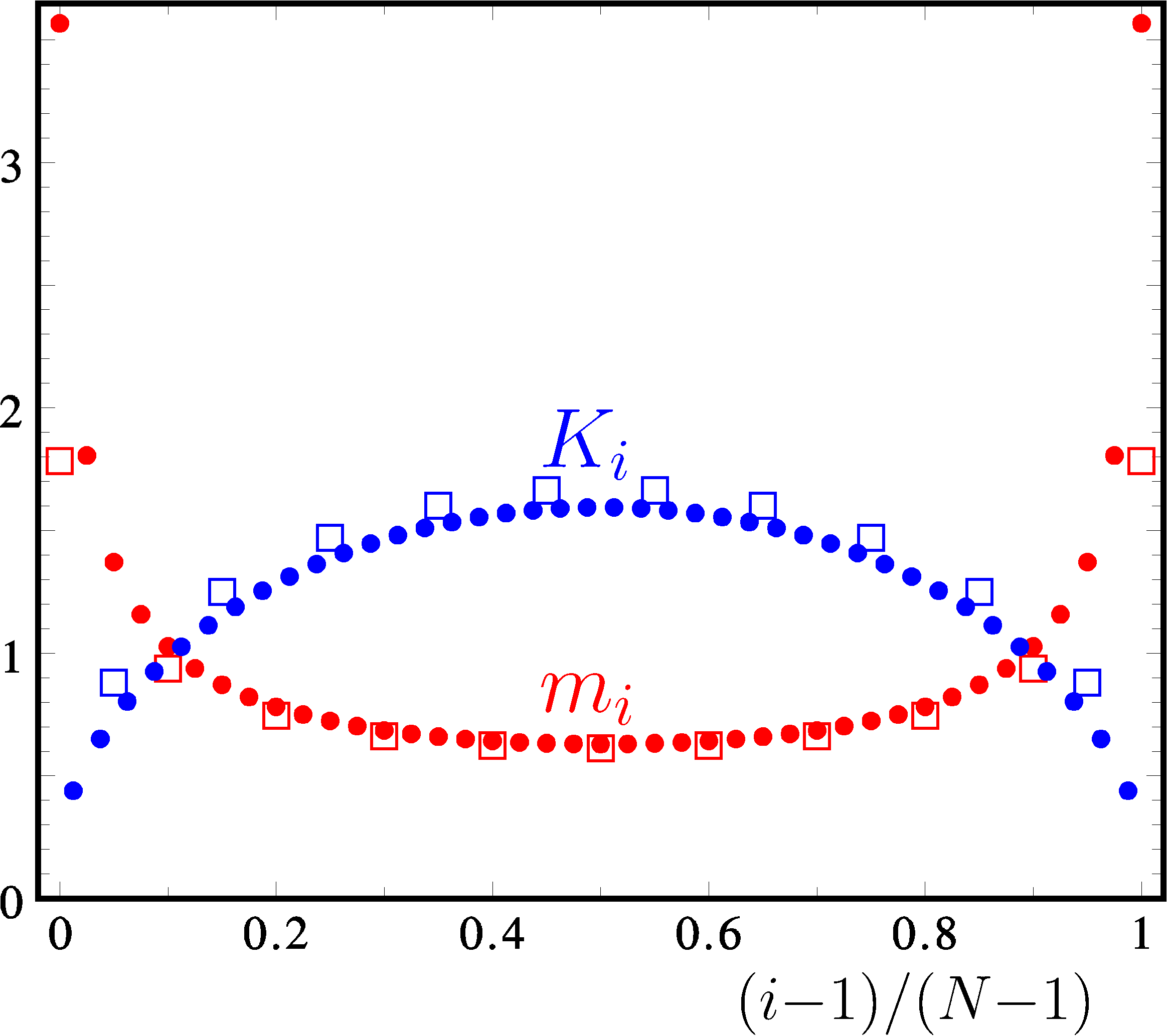
Figure 3: The sequence of masses $\{m_{i}\}$ and elastic constants $\{K_{i}\}$ as given by Eqs. (25) for chains of size $N=11$ (squares) and $N=41$ (bullets). Choosing $m_{1}=\sqrt{(N{-}1)/\pi}$, $\omega=\pi/(N{-}1)$, and the scaled variable $(i{-}1)/(N{-}1)$ allows to appreciate the overall scaling behavior VaiaS2020 . As the springs $K_{i}$ connect $m_{i}$ and $m_{i+1}$, for clarity they are plotted at $i{+}\frac{1}{2}$.

IV.2 General case: numerical solution

For a general choice of the eigenvalues (21), the inverse problem has to be faced numerically. To this purpose a good algorithm was proposed by de Boor and Golub deBoorG1978 (BG). It constructs the sequence of characteristic polynomials $\{\chi_{i}(\lambda)\}$  $(i=0,\,...,\,N)$ of the matrix $\bm{A}$ and its submatrices, using their orthogonality with respect to the internal product

$$\big{\langle}\chi,\tilde{\chi}\big{\rangle}\equiv\sum_{n=1}^{N}w_{n}~{}\chi(\lambda_{n})~{}\tilde{\chi}(\lambda_{n})~{},$$ (27)

where the weights are defined in terms of the required eigenvalues,

$$w_{n}=w\prod_{\begin{subarray}{c}m=1\\ m\neq{n}\end{subarray}}^{N}\big{|}\lambda_{n}-\lambda_{m}\big{|}^{-1}~{},$$ (28)

$w$ being an arbitrary positive constant. The property of orthogonality allows for the sequential construction of the polynomials,

$$\chi_{i+1}(\lambda)=(\lambda-a_{i+1})\,\chi_{i}(\lambda)-b_{i}^{2}\chi_{i-1}(\lambda)~{},$$ (29)

starting from $\chi_{0}(\lambda)=1$, $b_{0}(\lambda)\equiv{0}$, with the coefficients

$$a_{i+1}=\frac{\big{\langle}\lambda\,\chi_{i},\chi_{i}\big{\rangle}}{\big{\langle}\,\chi_{i},\chi_{i}\big{\rangle}}~{},~{}~{}~{}~{}~{}b_{i}^{2}=\frac{\big{\langle}\,\chi_{i},\chi_{i}\big{\rangle}}{\big{\langle}\,\chi_{i-1},\chi_{i-1}\big{\rangle}}$$ (30)

corresponding to the matrix elements one is looking for.

The numerical procedure starts by calculating and storing the weights (28) and proceeds in a simple manner with the iteration of Eqs. (29) and (30). It takes few lines of code, a clear example being found in Ref. BrudererFRBO2012 .

Once the matrix $\bm{A}$ is known, one has to reconstruct the sequence of masses and springs NylenU1997 . The masses are related to the components of the translation-mode eigenvector, $\bm{v}=\{U_{1i}\}$, since the identity

$$0=\bm{v}^{t}\bm{A}\,\bm{v}=\sum_{i=1}^{N-1}K_{i}\bigg{(}\frac{v_{i}}{\sqrt{m_{i}}}-\frac{v_{i+1}}{\sqrt{m_{i+1}}}\bigg{)}^{2}$$ (31)

entails the ratios $v_{i}/\sqrt{m_{i}}$ to be equal, hence $m_{i}=c\,v_{i}^{2}$, with $c$ a constant that is determined by the choice of $m_{1}$. The components of the equation $\bm{A}\,\bm{v}=\bm{0}$ define a recursion relation,

$$v_{i+1}=\frac{v_{i}\,a_{i}-v_{i-1}\,b_{i-1}}{b_{i}}~{},$$ (32)

that can be used to obtain the mass sequence starting from the given first mass (see Sec. II); in this way one has $v_{2}=a_{1}v_{1}/b_{1}$, then $v_{3}=(a_{1}a_{2}-v_{1}b_{1}^{2})/(b_{1}b_{2})$, and so on. Eventually, the elastic constants follow from Eq. (10), $K_{i}=c\,v_{i}v_{i+1}\,b_{i}$.

V Results and comparisons

The aim of this Section is to propose examples of perfectly transmitting chains, besides the exactly solved chain described by Eqs. (25), and compare their dynamics with that of the uniform chain and two kinds of quasi-uniform chains described in Ref. Vaia2018 : the first one with optimized $m_{1}$ and the second one with optimized $m_{1}$, $m_{2}$ and $K_{1}$. These optimized chains were shown to be able to rise the asymptotic transmission amplitude, which vanishes for the uniform chain, to $\alpha_{\infty}=0.847$ and to $\alpha_{\infty}=0.987$, respectively. Note that the uniform chain (with all $m_{i}=1$ and $K_{i}=1$) has the normal-mode frequencies

$$\omega_{n}=2\sin\frac{k_{n}}{2}~{},~{}~{}~{}k_{n}=\frac{\pi(n{-}1)}{N},~{}~{}~{}~{}n=1,...,N~{},$$ (33)

which are not commensurate, of course: the only low-$n$ modes are approximately spaced by $\omega=\pi/N$, while the spacing decreases for higher $n$. The parameters $k_{n}$ are quasi-wavevectors and lead to defining an analog of the group velocity Vaia2018 , $\partial\omega/\partial{k}=\cos\frac{k}{2}$, which is almost one at low $k$: indeed, it turns out that the maximal transmission amplitude occurs after the pulse has been traveling along the chain for a time $t^{*}\gtrsim\pi/\omega$ that is slightly larger than $N$. The fact that low-$k$ modes are almost commensurate means that long-wavelength pulses travel more coherently: this corresponds to the vibrating-string limit, $N\to\infty$ with $\omega_{k}\to{k}$. A travel time of order $N$ is also obtained when the only chain ends are modified in order to improve the transmission performance Vaia2018 .

Table 1 reports data concerning three chains of 11 masses, i.e., the uniform and the optimized quasi-uniform chains. The first row gives the “arrival time” $t^{*}$ where $\alpha_{N}(t)$ attains its maximum value $\alpha=\alpha_{{}_{N}}(t^{*})$: these quantities were calculated numerically. Besides the corresponding mirror-symmetric sequence of masses and springs, the table columns report the square-amplitudes of the normal modes, which are determined by the initial condition (17), as well as the “coherence factors” at arrival,

$$c_{n}=\cos[\pi(n{-}1){-}\omega_{n}t^{*}],~{}~{}~{}~{}n=1,...,N~{};$$ (34)

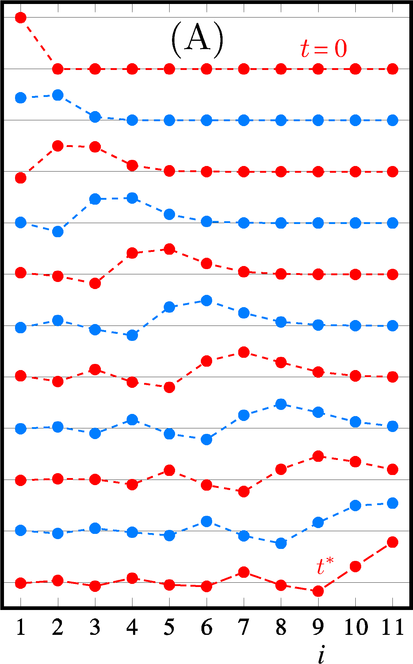
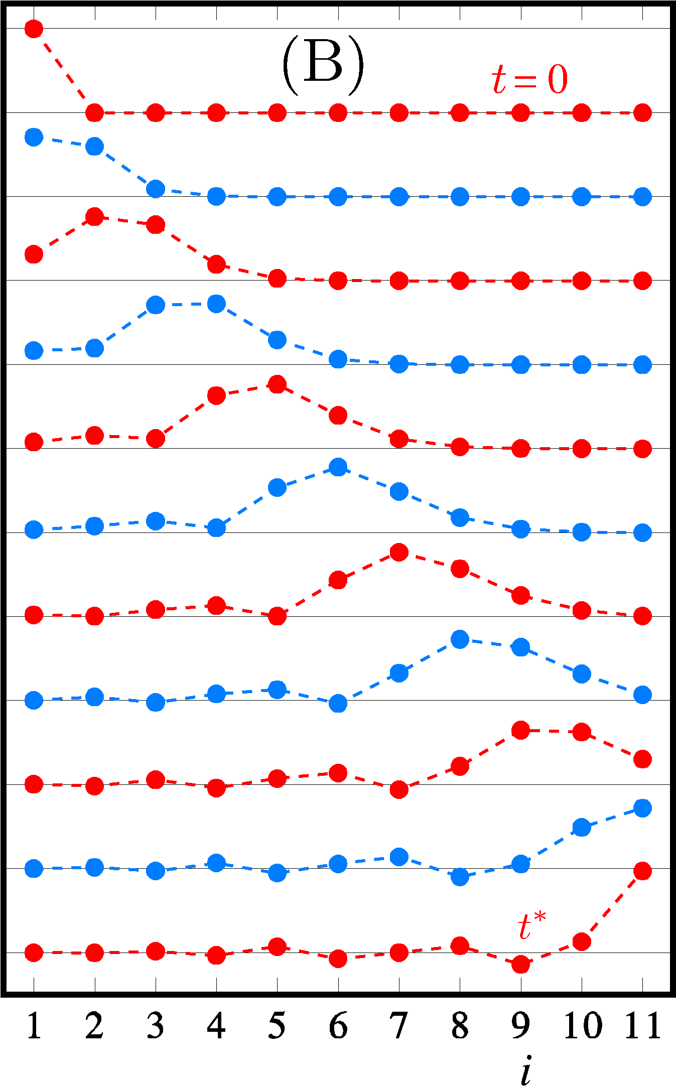
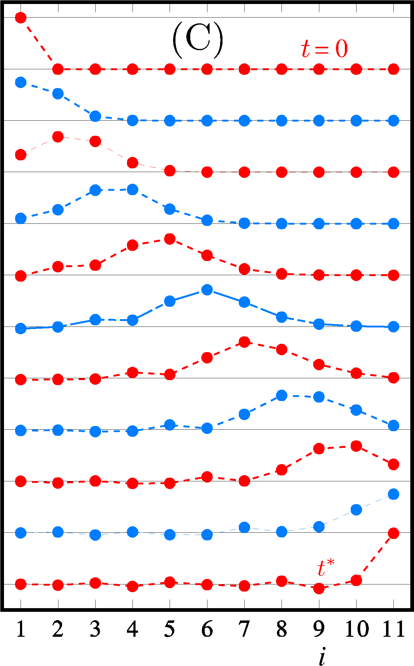
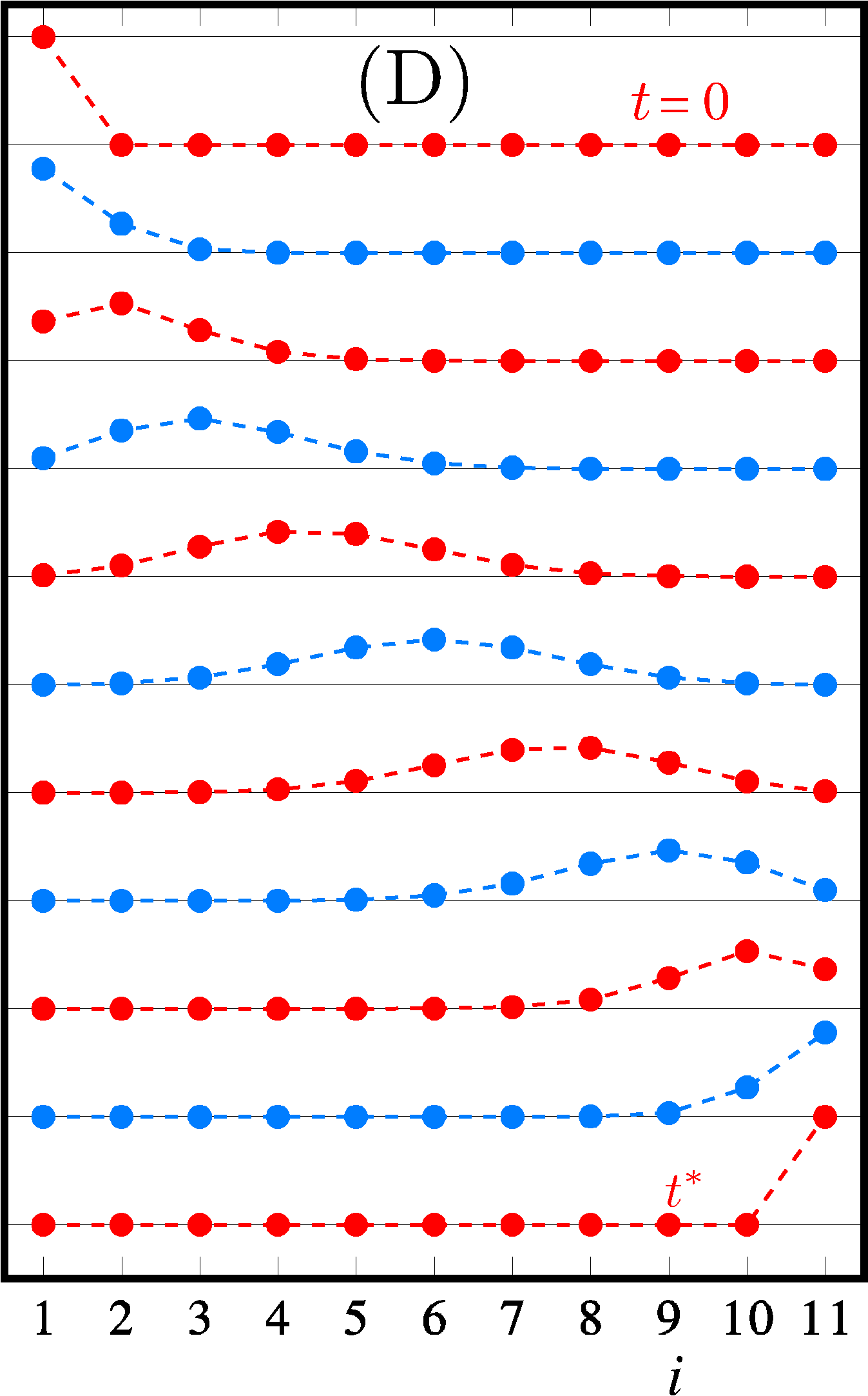
Figure 4: $N=11$ chain, snapshots of the dynamics at equal time intervals of $t^{*}/10$ between $0$ and $t^{*}$. The ordinate represents the momenta $p_{i}(t)$ of each mass as they evolve starting from the configuration (17). The first three panels correspond to the columns of Table 1, namely the uniform chain (A), the quasi-uniform chains with optimal extremal mass $m_{1}$ (B) and with 2 optimized extremal masses, $m_{1},~{}m_{2}$, and their spring $K_{1}$ (C); the last panel is the perfect chain (D) reported in Table 2. Animations are available as Supplemental Material supplmat.

the latter represent which fraction of the initial amplitude of the $n$th mode contributes to the overall transmitted amplitude $\alpha=\sum_{n}U_{n1}^{2}c_{n}$. It appears that higher-$n$ modes are less efficient (or less coherent), which explains the strategy used in the optimized chains: these perform better because the initial configuration gives larger weight to low-$n$ modes, which are reciprocally more coherent Vaia2018 . This improvement can be appreciated by looking at the dynamical evolution shown in the first three panels of Fig. 4, where the instantaneous momenta of all masses are reported at equal time intervals between $t=0$ and $t^{*}$ (as said in Sec. III, one can equivalently think of the elongations of each mass). See the Supplemental Material supplmat for animations.

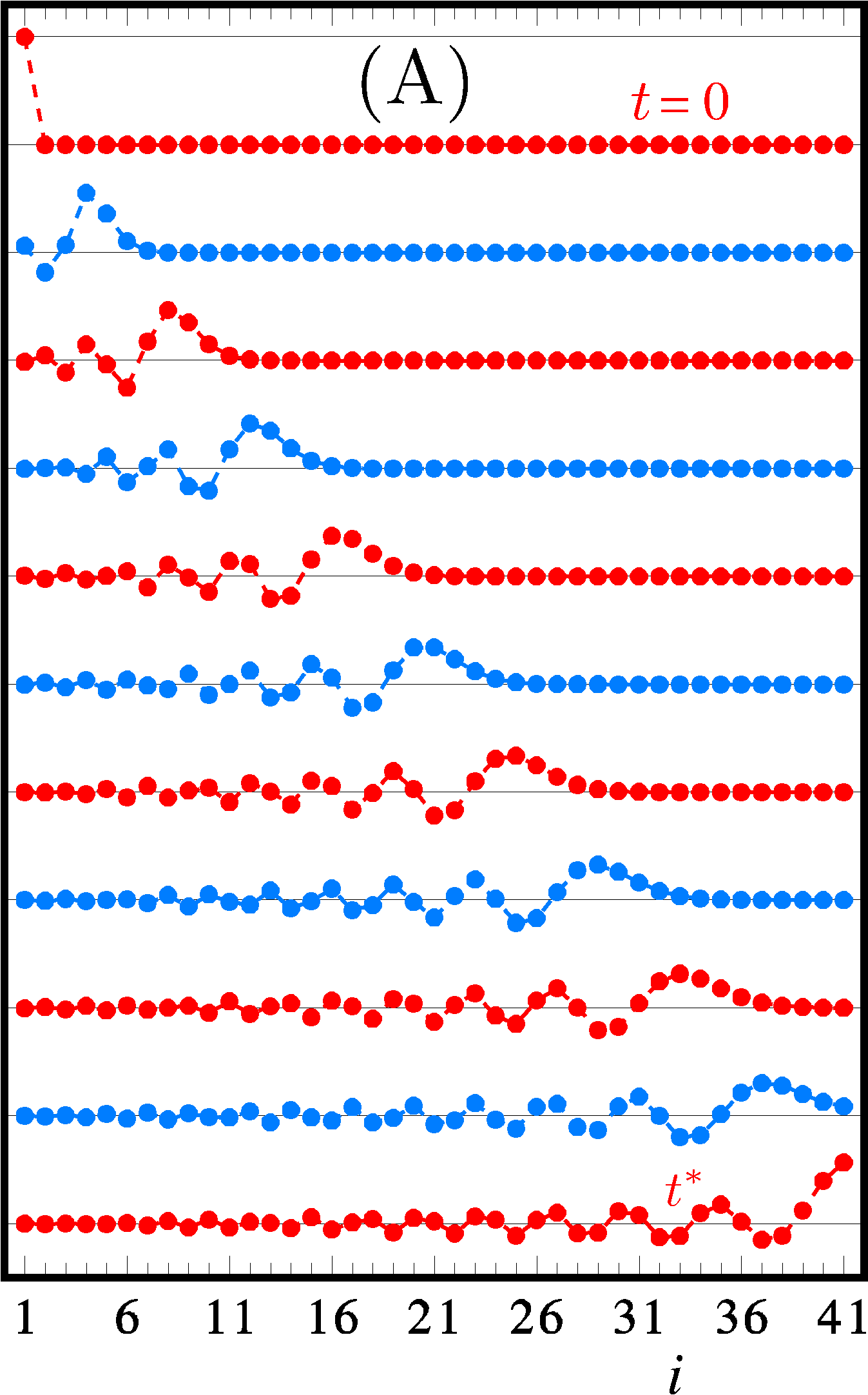
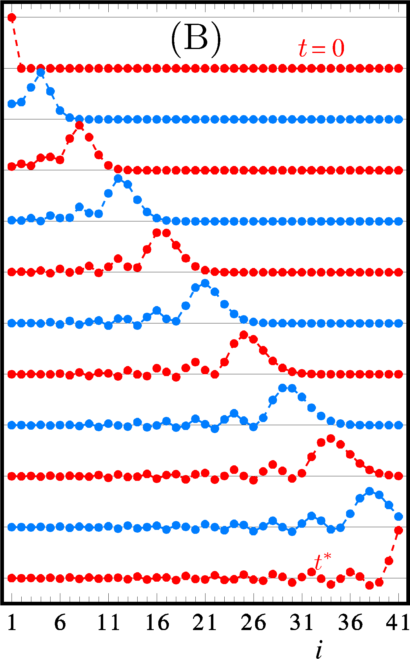
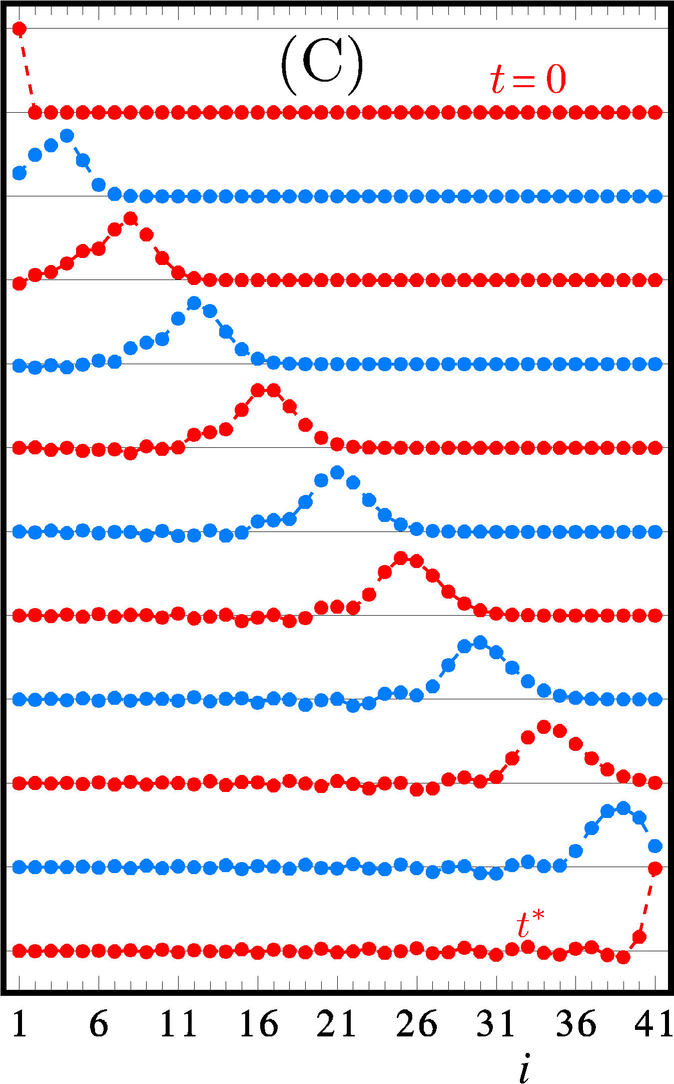
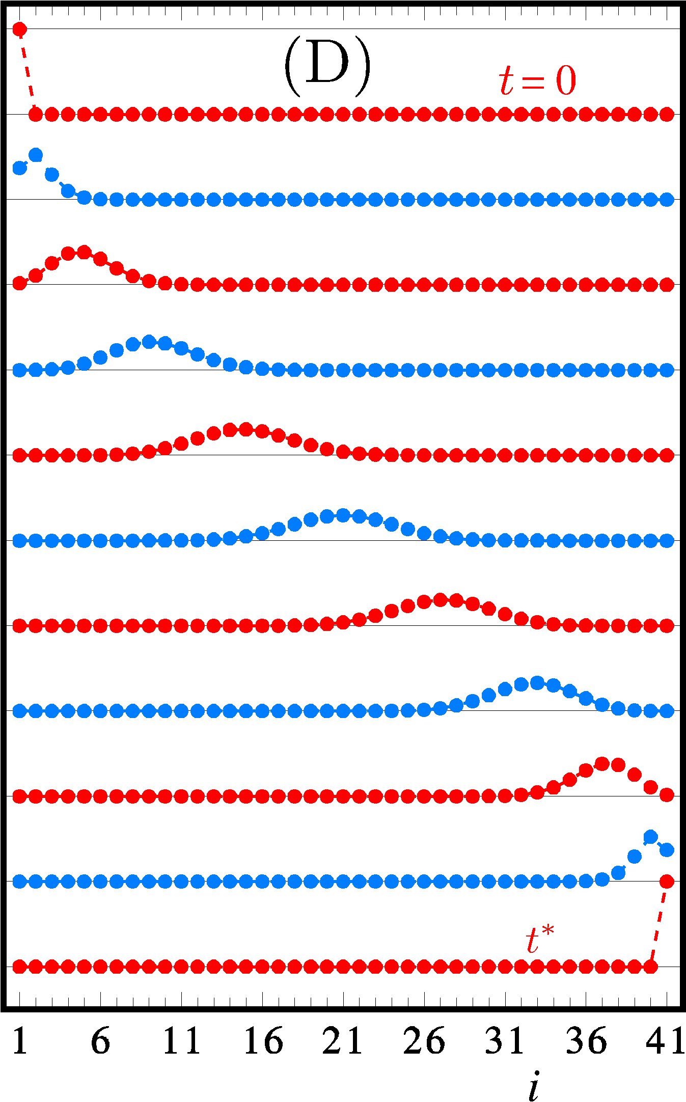
Figure 6: $N=41$ chain, snapshots of the dynamics at equal time intervals of $t^{*}/10$ between $0$ and $t^{*}$. The first three panels correspond to the columns of Table 3, namely the uniform chain (A), the quasi-uniform chains with optimal extremal mass $m_{1}$ (B) and with 2 optimized extremal masses, $m_{1},~{}m_{2}$, and their spring $K_{1}$ (C); the last panel is the perfect chain (D) reported in Table 4. Animations are available as Supplemental Material supplmat.

The same analysis applies to the longer chains, $N=41$, reported in Table 3 and in Fig. 6; there, the difference between the three cases is more evident. During the evolution the initial pulse appears to propagate along the chain with almost unit velocity, while at the arrival time an increasing amount of energy is transferred to the last mass, and not “dispersed” along the chain.

As discussed in Sec. III, all perfectly transmitting chains can be characterized by the sequence of odd coprime integers (22) which identifies the spectrum (21). In order to make a reasonable comparison with the above quasi-uniform chains, one can conveniently choose the parameter $\omega=\pi/(N{-}1)$, meaning that a pulse is expected to reach the opposite end at the transmission time $t^{*}=N{-}1$, equal to the chain length, hence with unit (average) velocity. Tables 2 and 4 report, besides the sequence (22), the corresponding values of masses and springs. In both tables, column (D) refers to the case of Eq. (5), yielding the analytic recipe (25), and the corresponding dynamics is shown in the fourth panels of Figs. 4 and 6. Columns (E) and (F) of the same tables report particular choices of the frequency sequence, among the infinite possible ones, which display less imbalanced (or “more uniform”) chains, as quantified in the last row. The reported data were calculated numerically by the method described in Sec. IV.

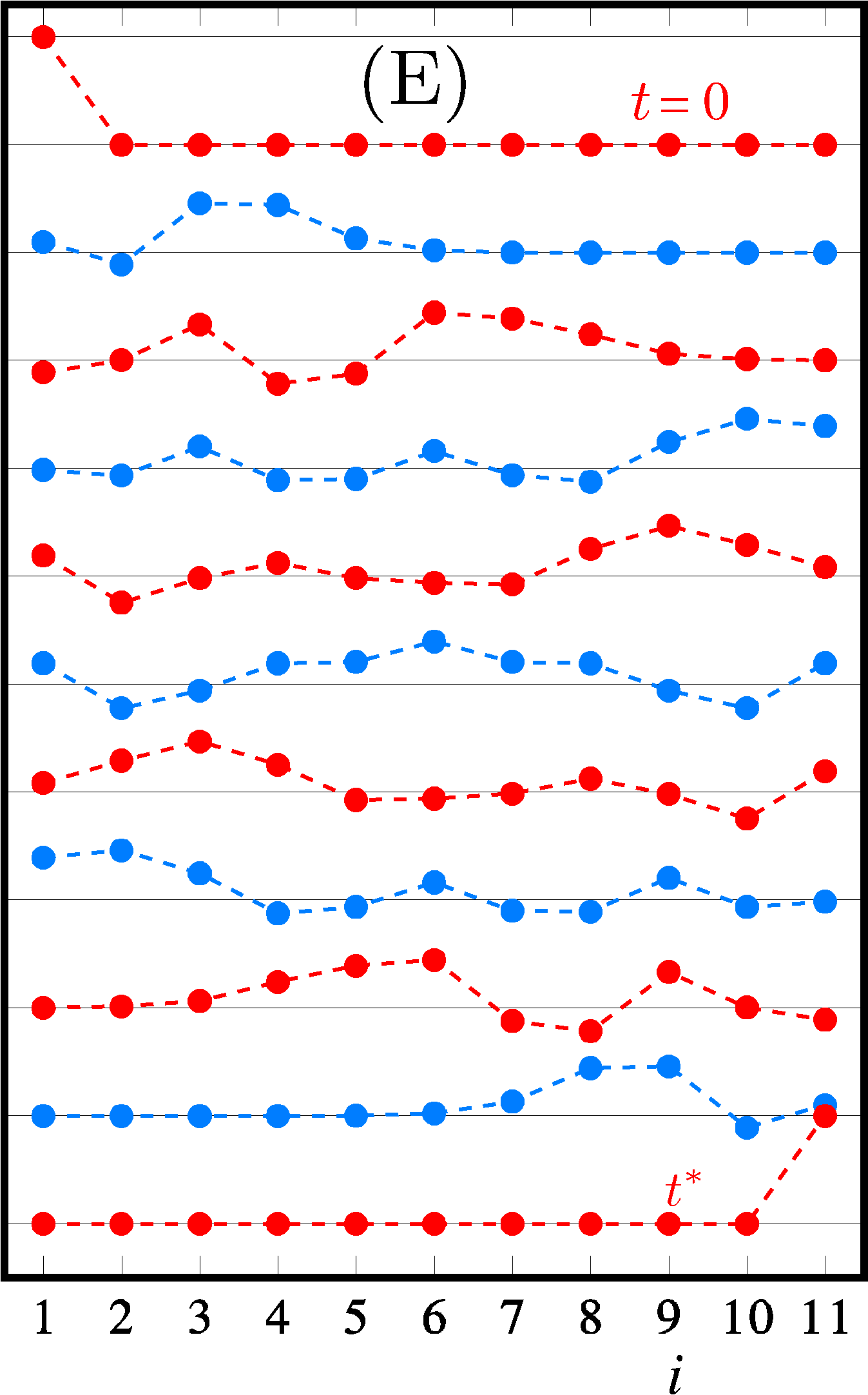
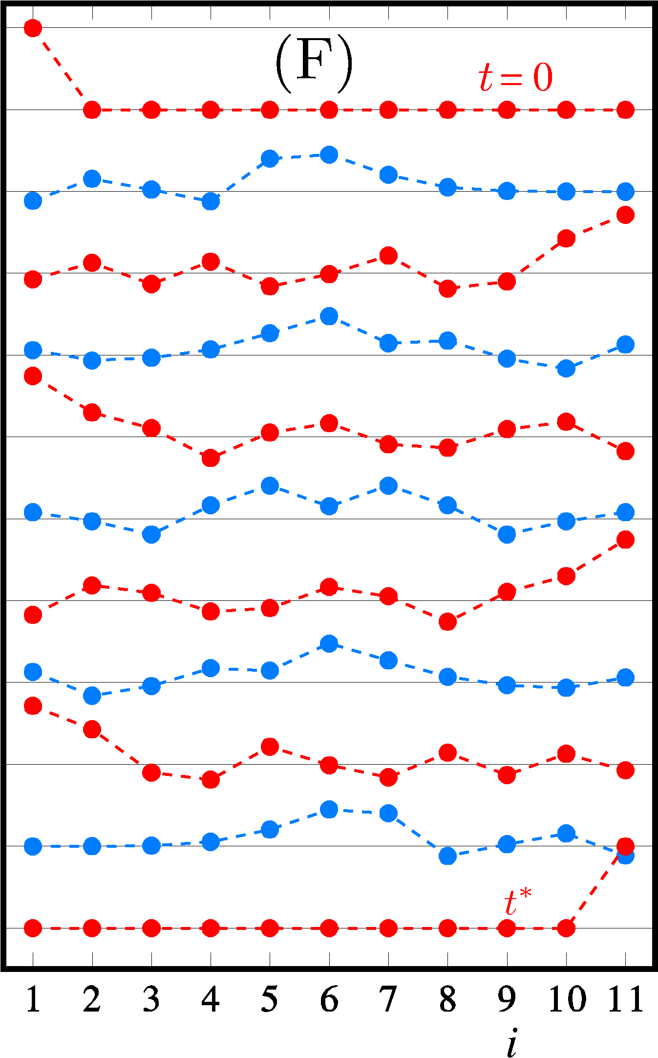
Figure 5: Snapshots of the dynamics at equal time intervals of $t^{*}/10$ between $0$ and $t^{*}=10$ for the two alternative $N=11$ perfectly transmitting chains (E) and (F) described in Table 2. Animations are available as Supplemental Material supplmat.

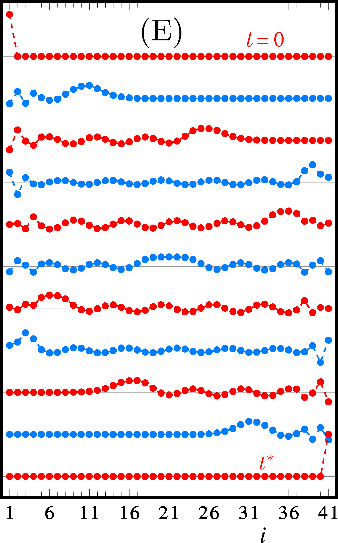
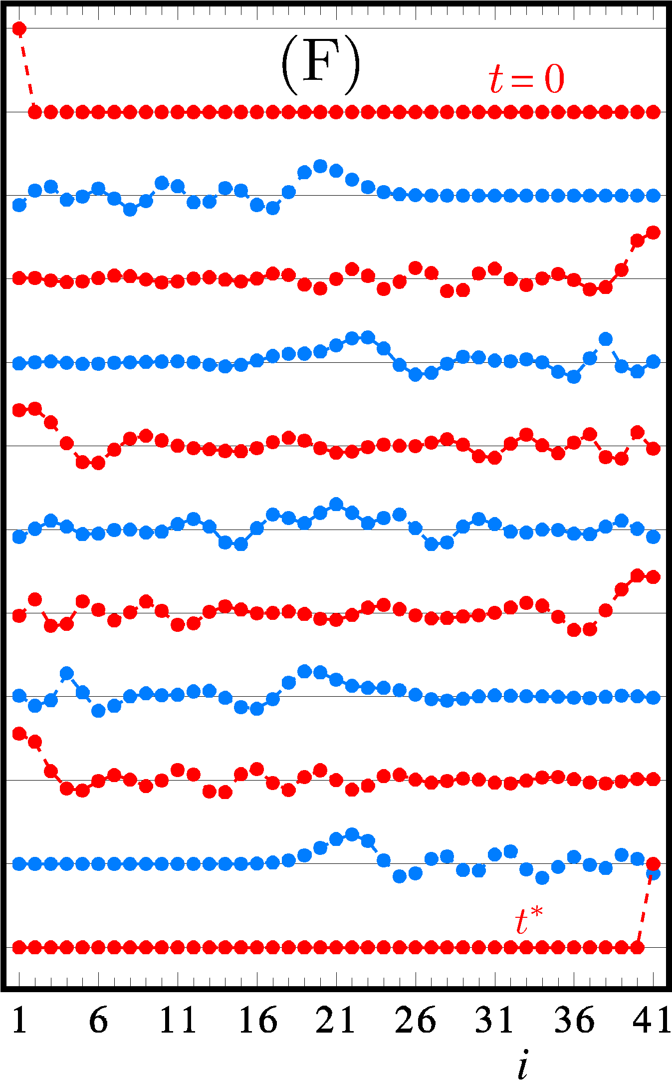
Figure 7: Snapshots of the dynamics at equal time intervals of $t^{*}/10$ between $0$ and $t^{*}=10$ for the two alternative $N=41$ perfectly transmitting chains (E) and (F) described in Table 4. Animations are available as Supplemental Material supplmat.

From the dynamics of these chains, Figs. 5 and 7, it appears that the behavior is more complex, since a few of the normal modes are tuned with a frequency spacing $\delta>1$. As a matter of fact, if all $\delta_{n}$ were equal to $\delta$, they would not be coprime and one should set $\omega\,\delta=\tilde{\omega}$, getting a shorter arrival time $\tilde{t}^{*}={t^{*}}/\delta$. In the cases shown in Figs. 4 and 6, with $\delta=3$ (E) and $\delta=5$ (F), one indeed observes a faster propagation of the initial pulse, as the incipient behavior is to yield large transmission at the earlier time $\tilde{t}^{*}$; however, at this time not all modes are coherent yet: this is particularly appreciable in Fig. 7, panel (F) at $t=t^{*}/5$; of course, perfect coherence among all modes will occur later at $t^{*}$.

VI Conclusions

Historically, the research aimed at obtaining efficient pulse transmission along one-dimensional mass-spring arrays mostly assumed translation-invariant (i.e., uniform) chains with nonelastic springs, as many nonlinear dynamic equations have been known to admit localized soliton-like solutions able to travel along the chain while preserving their shape.

At variance with this approach, in this paper uniformity is renounced instead of linearity, and it is shown how to characterize all mass-spring chains that yield perfect end-to-end pulse transmission, thus showing a dynamics analogous to that of a Newton’s cradle. In particular, all perfectly transmitting arrays of $N$ masses pairwise connected by $N\,{-}\,1$ springs are in one-to-one correspondence with the ordered sequences of coprime odd integers $(\delta_{1},...,\,\delta_{N-1})$. For the simplest sequence $(1,\,1,\,...,1)$ there exists an analytic recipe VaiaS2020 , while in the general case an efficient algorithm allows one to compute the mass-spring sequence numerically.

These “magic” chains can be used to build mechanical devices able, say, to efficiently transfer energy or momentum between the chain ends, whatever the chain length $N$. For instance, one can think of a desk toy that could replace the Newton cradle, like that shown in Fig. 1, the main difference being in the finite time required for a pulse to travel along the chain: in the ideal case where dissipation is neglected a pulse starting from one end can bounce back and forth indefinitely.

In the electrical circuit of Fig. 2, provided the capacitance-induction sequence is a “magic” one, a current pulse, generated by an external inductance coupled to $L_{1}$, would also bounce back and forth along the array.

One can imagine other applications, spanning from the macroscopic to the microscopic world CahillEtAl2003 ; NorrisLB2013 ; RammPH2014 . The versatility of the model (1) allows for many alternative implementations: basically, one could state that what is presented here constitutes a solution looking for a problem. A suggestion may be that some biologically active polymer chains could be close to some “magic” mass-spring sequence, enhancing their ability to transfer energy.

Appendix A Eqs. (23) entail Eq. (24)

Following Ref. VaiaS2020 , the proof by induction on $N$ starts from $N\,{=}\,1$, where the statement is trivially true, as $\bm{A}_{1}=[0]_{1}$ has the eigenvalue $\lambda_{1}=0$. Assuming that the statement holds true for dimension $N$, one has to show that the validity follows for $N+1$, i.e., that $\bm{A}_{N+1}$ has the $N$ eigenvalues of $\bm{A}_{N}$ plus the eigenvalue $\lambda_{N+1}=2N^{2}$.

The entries of $\bm{A}_{N+1}$ are

$$a_{i} =N+4(i{-}1)(N{+}1{-}i)~{}, i=1,\,...,\,N{+}1~{},$$ (35)

$$b_{i}^{2} =i\,(2i{-}1)\,(N{+}1{-}i)\,(2N{+}1{-}2i)~{}, i=1,\,...,\,N~{}.$$

It is simple algebra to verify that the tridiagonal matrix $2N^{2}-\bm{A}_{N+1}$, with diagonal elements

$$2N^{2}-a_{i}=N(N{-}1)+(N{+}2{-}2i)^{2}~{},$$ (36)

factorizes as $2N^{2}-\bm{A}_{N+1}=\bm{H}\bm{H}^{\rm T}$. The matrix

$$\bm{H}=\begin{bmatrix}h_{1}&0&\cdots&0\\ r_{1}&h_{2}&&\vdots\\ \vdots&&~{}\ddots&0\\ 0&\cdots&r_{N}&h_{N+1}\end{bmatrix}_{N+1}$$ (37)

is lower bidiagonal and has positive elements given by

$$h_{i}^{2} =(N{+}1{-}i)(2N{+}1{-}2i)~{}, i=1,\,...,\,N{+}1~{},$$ (38)

$$r_{i}^{2} =i\,(2i{-}1)~{}, i=1,\,...,\,N~{}.$$

The matrix $\bm{A}_{N+1}=2N^{2}-\bm{H}\bm{H}^{\rm T}$, has the same spectrum of the matrix

$$2N^{2}-\bm{H}^{\rm T}\bm{H}=\begin{bmatrix}&&&0\\ &~{}\bm{A}_{N}&&\vdots\\ &&&0\\ 0&\cdots&0&2N^{2}\end{bmatrix}_{N+1}~{};$$ (39)

hence, its eigenvalues are those of $\bm{A}_{N}$ plus the $(N+1)$th eigenvalue $2N^{2}$.

.

Table 1: Comparison of different mass-spring chains with $N=11$. The first column (A) refers to the uniform chain, the next two columns (B, C) to the optimized chains studied in Ref. Vaia2018 ; $t^{*}$ is the “arrival time” when the transmission amplitude $\alpha=\alpha_{{}_{N}}(t^{*})$ is maximal; $c_{n}=\cos[\pi(n{-}1){-}\omega_{n}t^{*}]$ is the coherence factor and $U_{n1}^{2}$ is the weight of each mode. Transmission is increasingly efficient from (A) to (C) because heavier coherence factors are closer to unity.

	(A) uniform				(B) optimal $m_{1}$				(C) optimal $m_{1},\,m_{2},\,K_{1}$
	$t^{*}=11.917$    $\alpha=0.787$				$t^{*}=13.039$    $\alpha=0.972$				$t^{*}=13.351$    $\alpha=0.989$
$i,n$	$m_{i}$	$K_{i}$	$c_{n}$	$U_{n1}^{2}$	$m_{i}$	$K_{i}$	$c_{n}$	$U_{n1}^{2}$	$m_{i}$	$K_{i}$	$c_{n}$	$U_{n1}^{2}$
1	1	1	1.0000	0.0909	2.4121	1	1.0000	0.1745	2.1259	0.7212	1.0000	0.1639
2	1	1	0.9688	0.1781	1	1	0.9902	0.3046	0.8606	1	0.9988	0.3084
3	1	1	0.9083	0.1674	1	1	0.9943	0.2121	1	1	0.9992	0.2418
4	1	1	0.8887	0.1504	1	1	0.9969	0.1311	1	1	0.9945	0.1467
5	1	1	0.9495	0.1287	1	1	0.9646	0.0781	1	1	0.9992	0.0723
6	1	1	0.9950	0.1039	1	1	0.9566	0.0462	1	1	0.9633	0.0338
7	1	1	0.6697	0.0780	1	1	0.9994	0.0269	1	1	0.9515	0.0167
8	1	1	0.3615	0.0531	1	1	0.8130	0.0150	1	1	0.9968	0.0089
9	1	1	0.9520	0.0314	1	1	0.1771	0.0077	1	1	0.4874	0.0048
10	1	1	0.6392	0.0144	1	1	0.9645	0.0032	0.8606	0.7212	0.9048	0.0022
11	1		0.0295	0.0037	2.4121		0.8030	0.0008	2.1259		0.2713	0.0006

Table 2: Comparison of different perfectly transmitting mass-spring chains with $N=11$. The first column (D) refers to the perfect chain VaiaS2020 with the spectrum (5), columns (E) and (F) are sample cases with different frequency spacings $\delta_{n}$, Eq.(22). The last row reports the ratio between largest and smallest values, quantifying the non-uniformity of the chain.

	(D)				(E)				(F)
$i,n$	$\delta_{n}$	$k_{n}$	$m_{i}$	$K_{i}$	$\delta_{n}$	$k_{n}$	$m_{i}$	$K_{i}$	$\delta_{n}$	$k_{n}$	$m_{i}$	$K_{i}$
1	1	0	1.0000	0.4935	3	0	1.0000	13.068	5	0	1.0000	39.020
2	1	1	0.5263	0.7013	3	3	1.0983	11.014	5	5	0.9636	28.190
3	1	2	0.4180	0.8250	3	6	0.8129	9.925	5	10	0.8206	27.888
4	1	3	0.3715	0.8983	3	9	1.0745	11.539	5	15	0.9779	27.903
5	1	4	0.3501	0.9329	3	12	0.7550	10.746	5	20	0.8471	29.662
6	1	5	0.3437	0.9329	1	15	1.0727	10.746	3	25	0.8905	29.662
7	1	6	0.3501	0.8983	3	16	0.7550	11.539	3	28	0.8471	27.903
8	1	7	0.3715	0.8250	1	19	1.0745	9.925	3	31	0.9779	27.888
9	1	8	0.4180	0.7013	1	20	0.8129	11.014	1	34	0.8206	28.190
10	1	9	0.5263	0.4935	1	21	1.0983	13.068	1	35	0.9636	39.020
11		10	1.0000			22	1.0000			36	1.0000
$\frac{\rm{max}}{\rm{min}}$			2.91	1.89			1.45	1.32			1.22	1.40

Table 3: Comparison of different mass-spring chains with $N=41$. The first column (A) refers to the uniform chain, the next two columns (B, C) to the optimized chains studied in Ref. Vaia2018 ; $t^{*}$ is the “arrival time” when the transmission amplitude $\alpha=\alpha_{{}_{N}}(t^{*})$ is maximal; $c_{n}=\cos[\pi(n{-}1){-}\omega_{n}t^{*}]$ is the coherence factor and $U_{n1}^{2}$ is the weight of each mode. Transmission is increasingly efficient from (A) to (C) because heavier coherence factors are closer to unity.

	(A) uniform				(B) optimal $m_{1}$				(C) optimal $m_{1},\,m_{2},\,K_{1}$
	$t^{*}=42.620$    $\alpha=0.5681$				$t^{*}=44.787$    $\alpha=0.9377$				$t^{*}=45.702$    $\alpha=0.9844$
$i,n$	$m_{i}$	$K_{i}$	$c_{n}$	$U_{n1}^{2}$	$m_{i}$	$K_{i}$	$c_{n}$	$U_{n1}^{2}$	$m_{i}$	$K_{i}$	$c_{n}$	$U_{n1}^{2}$
1	1	1	1.0000	0.0244	3.8133	1	1.0000	0.0818	3.2017	0.5255	1.0000	0.0713
2	1	1	0.9924	0.0487	1	1	0.9931	0.1568	0.7627	1	0.9988	0.1420
3	1	1	0.9709	0.0485	1	1	0.9798	0.1392	1	1	0.9974	0.1396
4	1	1	0.9391	0.0481	1	1	0.9734	0.1166	1	1	0.9986	0.1330
5	1	1	0.9024	0.0476	1	1	0.9790	0.0943	1	1	1.0000	0.1200
6	1	1	0.8673	0.0470	1	1	0.9911	0.0751	1	1	0.9970	0.1010
7	1	1	0.8404	0.0463	1	1	0.9995	0.0596	1	1	0.9914	0.0791
8	1	1	0.8276	0.0454	1	1	0.9965	0.0475	1	1	0.9901	0.0584
9	1	1	0.8331	0.0443	1	1	0.9803	0.0382	1	1	0.9951	0.0416
10	1	1	0.8585	0.0432	1	1	0.9549	0.0310	1	1	0.9999	0.0292
11	1	1	0.9011	0.0420	1	1	0.9285	0.0254	1	1	0.9955	0.0205
12	1	1	0.9518	0.0406	1	1	0.9104	0.0210	1	1	0.9779	0.0146
13	1	1	0.9924	0.0392	1	1	0.9082	0.0175	1	1	0.9511	0.0106
14	1	1	0.9929	0.0377	1	1	0.9253	0.0147	1	1	0.9250	0.0078
15	1	1	0.9120	0.0360	1	1	0.9579	0.0124	1	1	0.9111	0.0059
16	1	1	0.7039	0.0344	1	1	0.9912	0.0105	1	1	0.9179	0.0045
17	1	1	0.3389	0.0326	1	1	0.9957	0.0089	1	1	0.9463	0.0035
18	1	1	0.1606	0.0309	1	1	0.9247	0.0077	1	1	0.9838	0.0028
19	1	1	0.6774	0.0290	1	1	0.7211	0.0066	1	1	0.9989	0.0023
20	1	1	0.9866	0.0272	1	1	0.3416	0.0056	1	1	0.9363	0.0019
21	1	1	0.8355	0.0253	1	1	0.1937	0.0048	1	1	0.7231	0.0016
22	1	1	0.1560	0.0235	1	1	0.7377	0.0042	1	1	0.3024	0.0013
23	1	1	0.6933	0.0216	1	1	0.9999	0.0036	1	1	0.2922	0.0011
24	1	1	0.9778	0.0198	1	1	0.6837	0.0031	1	1	0.8459	0.0009
25	1	1	0.2445	0.0179	1	1	0.1784	0.0026	1	1	0.9659	0.0008
26	1	1	0.8221	0.0162	1	1	0.9385	0.0022	1	1	0.3595	0.0007
27	1	1	0.7592	0.0144	1	1	0.6993	0.0019	1	1	0.6402	0.0006
28	1	1	0.5289	0.0127	1	1	0.4688	0.0016	1	1	0.9520	0.0005
29	1	1	0.8711	0.0111	1	1	0.9566	0.0013	1	1	0.0558	0.0005
30	1	1	0.5475	0.0096	1	1	0.2207	0.0011	1	1	0.9977	0.0004
31	1	1	0.7266	0.0082	1	1	0.9635	0.0009	1	1	0.0585	0.0004
32	1	1	0.8673	0.0068	1	1	0.4295	0.0007	1	1	0.9962	0.0003
33	1	1	0.1124	0.0056	1	1	0.7364	0.0006	1	1	0.3627	0.0003
34	1	1	0.9158	0.0044	1	1	0.9210	0.0005	1	1	0.7009	0.0002
35	1	1	0.8717	0.0034	1	1	0.1569	0.0003	1	1	0.9772	0.0002
36	1	1	0.2512	0.0025	1	1	0.6621	0.0003	1	1	0.4694	0.0002
37	1	1	0.4161	0.0018	1	1	0.9951	0.0002	1	1	0.2383	0.0001
38	1	1	0.8357	0.0011	1	1	0.8706	0.0001	1	1	0.7394	0.0001
39	1	1	0.9895	0.0006	1	1	0.5464	0.0001	1	1	0.9604	0.0001
40	1	1	0.9860	0.0003	1	1	0.2337	0.0000	0.7627	0.5255	0.9992	0.0000
41	1		0.9377	0.0001	3.8133		0.0304	0.0000	3.2017		0.9728	0.0000

Table 4: Comparison of different perfectly transmitting mass-spring chains with $N=41$. The first column (D) refers to the perfect chain VaiaS2020 with the spectrum (5), columns (E) and (F) are sample cases with different frequency spacings $\delta_{n}$, Eq.(22). The last row reports the ratio between largest and smallest values, quantifying the non-uniformity of the chain.

	(D)				(E)				(F)
$i,n$	$\delta_{n}$	$k_{n}$	$m_{i}$	$K_{i}$	$\delta_{n}$	$k_{n}$	$m_{i}$	$K_{i}$	$\delta_{n}$	$k_{n}$	$m_{i}$	$K_{i}$
1	1	0	1.0000	0.1234	3	0	1.0000	6.413	5	0	1.0000	22.240
2	1	1	0.5063	0.1827	3	3	1.2055	2.677	5	5	1.0582	14.851
3	1	2	0.3847	0.2254	3	6	1.0458	3.775	5	10	1.0080	20.927
4	1	3	0.3248	0.2595	3	9	0.8147	4.351	5	15	0.8424	15.130
5	1	4	0.2881	0.2879	3	12	0.6823	6.066	5	20	0.7170	20.767
6	1	5	0.2630	0.3123	3	15	0.4889	7.352	5	25	0.8666	23.079
7	1	6	0.2445	0.3334	3	18	0.4585	6.310	5	30	0.6978	21.220
8	1	7	0.2305	0.3519	3	21	0.5433	7.094	5	35	0.6676	20.974
9	1	8	0.2194	0.3681	3	24	0.4688	7.156	5	40	0.6944	21.126
10	1	9	0.2105	0.3824	3	27	0.4619	6.484	5	45	0.7305	23.319
11	1	10	0.2032	0.3949	3	30	0.5269	6.960	3	50	0.7411	22.081
12	1	11	0.1973	0.4059	3	33	0.4952	7.083	5	53	0.6724	20.295
13	1	12	0.1924	0.4154	3	36	0.4399	6.955	5	58	0.6963	21.596
14	1	13	0.1884	0.4235	3	39	0.4906	7.097	5	63	0.7353	22.397
15	1	14	0.1851	0.4303	3	42	0.5095	6.891	5	68	0.7169	22.708
16	1	15	0.1824	0.4360	1	45	0.4543	6.973	5	73	0.6856	21.483
17	1	16	0.1803	0.4404	1	46	0.4654	7.369	5	78	0.6667	21.049
18	1	17	0.1787	0.4437	1	47	0.4993	7.038	3	83	0.7254	22.458
19	1	18	0.1776	0.4459	3	48	0.4667	6.760	3	86	0.7442	22.036
20	1	19	0.1770	0.4470	3	51	0.4656	7.330	3	89	0.6879	21.780
21	1	20	0.1767	0.4470	3	54	0.4898	7.330	3	92	0.6675	21.780
22	1	21	0.1770	0.4459	3	57	0.4656	6.760	3	95	0.6879	22.036
23	1	22	0.1776	0.4437	3	60	0.4667	7.038	3	98	0.7442	22.458
24	1	23	0.1787	0.4404	3	63	0.4993	7.369	3	101	0.7254	21.049
25	1	24	0.1803	0.4360	3	66	0.4654	6.973	3	104	0.6667	21.483
26	1	25	0.1824	0.4303	3	69	0.4543	6.891	3	107	0.6856	22.708
27	1	26	0.1851	0.4235	3	72	0.5095	7.097	3	110	0.7169	22.397
28	1	27	0.1884	0.4154	3	75	0.4906	6.955	3	113	0.7353	21.596
29	1	28	0.1924	0.4059	3	78	0.4399	7.083	3	116	0.6963	20.295
30	1	29	0.1973	0.3949	3	81	0.4952	6.960	3	119	0.6724	22.081
31	1	30	0.2032	0.3824	3	84	0.5269	6.484	3	122	0.7411	23.319
32	1	31	0.2105	0.3681	1	87	0.4619	7.156	3	125	0.7305	21.126
33	1	32	0.2194	0.3519	1	88	0.4688	7.094	3	128	0.6944	20.974
34	1	33	0.2305	0.3334	3	89	0.5433	6.310	3	131	0.6676	21.220
35	1	34	0.2445	0.3123	1	92	0.4585	7.352	1	134	0.6978	23.079
36	1	35	0.2630	0.2879	1	93	0.4889	6.066	3	135	0.8666	20.767
37	1	36	0.2881	0.2595	1	94	0.6823	4.351	1	138	0.7170	15.130
38	1	37	0.3248	0.2254	1	95	0.8147	3.775	1	139	0.8424	20.927
39	1	38	0.3847	0.1827	1	96	1.0458	2.677	1	140	1.0080	14.851
40	1	39	0.5063	0.1234	1	97	1.2055	6.413	1	141	1.0582	22.240
41		40	1.0000			98	1.0000			142	1.0000
$\frac{\rm{max}}{\rm{min}}$			5.66	3.62			2.74	2.75			1.59	1.57

References

- (1) F. Herrmann and P. Schmälzle, Simple explanation of a well-known collision experiment, Am. J. Phys. 49, 761 (1981).
- (2) D. G. Cahill, W. K. Ford, K. E. Goodson, G. D. Mahan, A. Majumdar, H. J. Maris, R. Merlin, and S. R. Phillpot, Nanoscale thermal transport. J. Appl. Phys. 93, 793 (2003).
- (3) P. M. Norris, N. Q. Le, and C. H. Baker, Tuning Phonon Transport: From Interfaces to Nanostructures, J. Heat Transfer 135, 061604 (2013).
- (4) M. Ramm, T. Pruttivarasin, and H. Häffner, Energy transport in trapped ion chains, New J. Phys. 16, 063062 (2014).
- (5) F. Herrmann and M. Seitz, How does the ball-chain work?, Am. J. Phys. 50, 977 (1982).
- (6) S. Hutzler, G. Delaney, D. Weaire, and F. MacLeod, Rocking Newton’s cradle, Am. J. Phys. 72, 1508 (2004).
- (7) T. Kinoshita, T. Wenger, and D. S. Weiss, A quantum Newton’s cradle, Nature 440, 900 (2006).
- (8) C. Kittel, Introduction to Solid State Physics (Wiley, New York, 1953).
- (9) E. Fermi, J. Pasta, and S. Ulam, Studies of nonlinear problems, Los Alamos Document LA-1940 (1955).
- (10) T. Dauxois, M. Peyrard, Physics of Solitons (Cambridge University Press, Cambridge, 2006).
- (11) R. Vaia, Almost-dispersionless pulse transport in long quasiuniform spring-mass chains: A different kind of Newton’s cradle, Phys. Rev. E 97, 043001 (2018).
- (12) B. N. Parlett, The Symmetric Eigenvalue Problem (SIAM, Philadelphia, 1998).
- (13) The integers must be all different, otherwise at least one elastic constant would vanish as a consequence of frequency degeneration Parlett1998 , and the chain would be split into shorter independent chains.
- (14) H. Hochstadt, On some inverse problems in matrix theory, Arch. Math. 18 (1967) 201-207.
- (15) O. H. Hald, Inverse eigenvalue problems for Jacobi matrices, Linear Algebra Appl. 14 (1976) 63-85.
- (16) C. de Boor and G. H. Golub, The numerically stable reconstruction of a Jacobi matrix from spectral data, Linear Algebr. Appl. 21, 245 (1978).
- (17) P. Nylen and F. Uhlig, Inverse eigenvalue problems associated with spring-mass systems, Linear Algebra Appl. 254, 409 (1997).
- (18) R. Vaia and L. Spadini, Persymmetric Jacobi matrices with square-integer eigenvalues and dispersionless mass-spring chains, Linear Algebra Appl. 585, 164 (2020).
- (19) F. P. Gantmacher and M. G. Krein, Oscillation matrices and kernels and small vibrations of mechanical systems (AMS Chelsea Publishing, Providence, RI 2002) [Moscow, 1950 (Russian)].
- (20) A. Cantoni and P. Butler, Eigenvalues and eigenvectors of symmetric centrosymmetric matrices, Linear Algebra Appl. 13, 275 (1976).
- (21) It is to be noted that periodicity occurs for any set of integers , without the parity constraint.
- (22) M. Bruderer, K. Franke, S. Ragg, W. Belzig, and D. Obreschkow, Exploiting boundary states of imperfect spin chains for high-fidelity state transfer, Phys. Rev. A 85, 022312 (2012).