A Bayesian Hierarchical Score for Structure Learning from Related Data Sets

Abstract

Score functions for learning the structure of Bayesian networks in the literature assume that data are a homogeneous set of observations; whereas it is often the case that they comprise different related, but not homogeneous, data sets collected in different ways. In this paper we propose a new Bayesian Dirichlet score, which we call Bayesian Hierarchical Dirichlet (BHD). The proposed score is based on a hierarchical model that pools information across data sets to learn a single encompassing network structure, while taking into account the differences in their probabilistic structures. We derive a closed-form expression for BHD using a variational approximation of the marginal likelihood, we study the associated computational cost and we evaluate its performance using simulated data. We find that, when data comprise multiple related data sets, BHD outperforms the Bayesian Dirichlet equivalent uniform (BDeu) score in terms of reconstruction accuracy as measured by the Structural Hamming distance, and that it is as accurate as BDeu when data are homogeneous. This improvement is particularly clear when either the number of variables in the network or the number of observations is large. Moreover, the estimated networks are sparser and therefore more interpretable than those obtained with BDeu thanks to a lower number of false positive arcs.

1 Introduction

Investigating challenging problems at the forefront of science increasingly requires large amounts of data that can only be gathered through collaborations between several institutions. This naturally leads to heterogeneous data sets that are in fact the collation of related, but not identical, subsets of data that will necessarily differ in the details of how they are collected. Examples can be found in multi-centre clinical trials, in which protocols are applied in slightly different ways to different patient populations [1, 2]; population genetics, which studies the architecture of phenotypic traits across populations and their evolution [3, 4, 5, 6]; ecology and environmental sciences, which produce different patterns of measurement errors and limitations in different environments [7, 8, 9]. A common goal in analysing these complex data is to construct a mechanistic model that elucidates the interplay between different elements under investigation, either as a step towards building a causal model or to perform accurate prediction from a purely probabilistic perspective.

The task of efficiently modelling such related data sets is usually tackled by hierarchical models [10], which pool the information common to the different subsets of the data while encoding the information that is specific to each subset. For instance multilevel regression models estimate the conditional distribution of the response variables in these cases.

Bayesian networks (BNs) [11] provide a rigorous approach for modelling joint distributions, by representing variables as nodes and probabilistic dependencies as arcs in a graph. They can be used for both causal and predictive modelling. To the best of our knowledge, however, no method has been proposed in the literature to combine these two approaches to learn a single BN structure from a set of related data sets and get the best of both worlds.

Available methods focus on learning an ensemble of BNs that have similar structures by penalising differences in their arc sets [12, 13]. Parameter learning from related data sets has been investigated in [14] for Gaussian BNs and in [15] for discrete BNs. However, they only consider a naive Bayes structure and they initialise their hyperprior with maximum likelihood point estimates.

In this paper, we show how to learn the structure of a BN from related data sets, containing the same variables, by building on our previous work on parameter learning in [16]. The proposed approach is particularly suited to deal with multiple related data sets characterised by few observations per data set or by an unbalanced number of observations across data sets. In these settings, it is important to share information across data sets to obtain robust estimates of both the parameters and the structure of the BN. First, we briefly introduce BNs and hierarchical models in the context of discrete data as well as prior work on parameter learning from related data sets in Section 2. We propose a score function for related data sets in Section 3 and we study the associated computational complexity in both a theoretical and empirical way in Section 4. Then, we show an example of structure learning by means of BHD in Section 5 and we study its performance on different simulation studies in Section 6. Finally, we discuss our results and possible future research directions in Section 7.

2 Background and Notation

Bayesian networks (BNs) are a class of graphical models that use a directed acyclic graph (DAG) $\mathcal{G}$ to model a set of random variables $\mathbf{X}=\{X_{1},\ldots,X_{N}\}$: each node is associated with one $X_{i}\in\mathbf{X}$ and arcs represent direct dependence relationships. Graphical separation of two nodes implies the conditional independence of the corresponding random variables. In principle, there are many possible choices for the joint distribution of $\mathbf{X}$; literature has focused mostly on discrete BNs [17], in which both $\mathbf{X}$ and the $X_{i}$ are categorical (multinomial) random variables. Other possibilities include Gaussian BNs and conditional linear Gaussian BNs [18], which include both discrete and Gaussian BNs as particular cases.

The task of learning a BN from a data set $\mathcal{D}$ of $n$ observations is performed in two steps in an inherently Bayesian fashion:

$$\underbrace{\operatorname{P}(\mathcal{G},\Theta\operatorname{\mid}\mathcal{D})}_{\text{learning}}=\underbrace{\operatorname{P}(\mathcal{G}\operatorname{\mid}\mathcal{D})}_{\text{structure learning}}\cdot\underbrace{\operatorname{P}(\Theta\operatorname{\mid}\mathcal{G},\mathcal{D})}_{\text{parameter learning}},$$ (1)

where $\Theta$ are the parameters of $\mathbf{X}$. Structure learning consists in finding the DAG $\mathcal{G}$ that encodes the dependence structure of the data. In this paper we will focus on score-based algorithms, which are typically heuristic search algorithms that use a goodness-of-fit score such as BIC [19] or the Bayesian Dirichlet equivalent uniform (BDeu) marginal likelihood [17] to find an optimal $\mathcal{G}$. Parameter learning involves the estimation of the parameters $\Theta$ given the DAG $\mathcal{G}$ learned in the first step. Thanks to the Markov property, this step is computationally efficient because if the data are complete the global distribution of $\mathbf{X}$ decomposes into

$$\operatorname{P}(\mathbf{X}\operatorname{\mid}\mathcal{G})=\prod_{i=1}^{N}\operatorname{P}(X_{i}\operatorname{\mid}\Pi_{X_{i}})$$ (2)

and the local distribution associated with each node $X_{i}$ depends only on the configurations of its parents $\Pi_{X_{i}}$. If we estimate the parameters $\Theta=\{\Theta_{X_{1}},\ldots,\Theta_{X_{N}}\}$ in such a way that they are independent across local distributions, parameter learning simplifies into a collection of low-dimensional estimation problems for the $\Theta_{X_{i}}$ associated with each $X_{i}\operatorname{\mid}\Pi_{X_{i}}$ given the data available for those variables.

2.1 Classic Multinomial-Dirichlet Parameterisation

In the case of discrete BNs, we assume that each $X_{i}\operatorname{\mid}\Pi_{X_{i}}$ follows a categorical distribution for each configuration of $\Pi_{X_{i}}$. Hence the parameters of $X_{i}\operatorname{\mid}\Pi_{X_{i}}$ are the conditional probabilities $\boldsymbol{\theta}_{X_{i}\operatorname{\mid}\Pi_{X_{i}}}=\{\boldsymbol{\theta}_{X_{i}\operatorname{\mid}j},j=1,\ldots,|\Pi_{X_{i}}|\}$, whose $k$th element corresponds to $\operatorname{P}(X_{i}=k\operatorname{\mid}\Pi_{X_{i}}=j)$, for which we assume a conjugate Dirichlet prior:

$$\left.\boldsymbol{\theta}_{X_{i}\operatorname{\mid}\Pi_{X_{i}}}\,\right|\boldsymbol{\alpha}_{i} \sim\operatorname{Dirichlet}(\boldsymbol{\alpha}_{i})$$

$$X_{i}\left|\,\Pi_{X_{i}},\boldsymbol{\theta}_{X_{i}\operatorname{\mid}\Pi_{X_{i}}}\right. \sim\operatorname{Categorical}\left(\boldsymbol{\theta}_{X_{i}\operatorname{\mid}\Pi_{X_{i}}}\right),$$ (3)

where $\boldsymbol{\alpha}_{i}=\{\alpha_{ijk},j=1,\ldots,|\Pi_{X_{i}}|;k=1,\ldots,|X_{i}|\}$, with $i=1,\ldots,N$, is a hyperparameter vector defined over a simplex with sum $\sum_{jk}\alpha_{ijk}=s_{i}>0$. The posterior estimator of $\boldsymbol{\theta}_{X_{i}\operatorname{\mid}\Pi_{X_{i}}}$ is:

$$\left[\boldsymbol{\widehat{\theta}}_{X_{i}\operatorname{\mid}j}\right]_{k}=\frac{\alpha_{ijk}+n_{ijk}}{\alpha_{ij}+n_{ij}}, n_{ij}=\sum\nolimits_{k}n_{ijk},\ \ \alpha_{ij}=\sum\nolimits_{k}\alpha_{ijk},$$ where (4)

and $n_{ijk}$ represents the number of observations for which $X_{i}=k$ and $\Pi_{X_{i}}=j$. It is common to set $\alpha_{ijk}=s_{i}/(|X_{i}||\Pi_{X_{i}}|)$ with the same imaginary sample size $s_{i}=s$ for all $X_{i}$.

In the context of structure learning, we have $\operatorname{P}(\mathcal{G}\operatorname{\mid}\mathcal{D})\propto\operatorname{P}(\mathcal{D}\operatorname{\mid}\mathcal{G})\operatorname{P}(\mathcal{G})$ and we can use $\operatorname{P}(\mathcal{D}\operatorname{\mid}\mathcal{G})$ as a score function. (Implicitly, we are saying that $\operatorname{P}(\mathcal{G})\propto 1$ by disregarding it while still searching for the maximum a posteriori DAG.) Assuming positivity ($\boldsymbol{\theta}_{X_{i}\operatorname{\mid}\Pi_{X_{i}}}>0$), parameter independence (columns of $\boldsymbol{\theta}_{X_{i}\operatorname{\mid}\Pi_{X_{i}}}$ associated with different parent configurations are independent), parameter modularity ($\boldsymbol{\theta}_{X_{i}\operatorname{\mid}\Pi_{X_{i}}}$ associated with different nodes are independent) and complete data, [17] derived a closed form expression for $\operatorname{P}(\mathcal{D}\operatorname{\mid}\mathcal{G})$ known as the Bayesian Dirichlet (BD) family of scores:

$$\operatorname{BD}(\mathcal{G},\mathcal{D};\boldsymbol{\alpha})=\prod_{i=1}^{N}\operatorname{BD}\left(X_{i}\operatorname{\mid}\Pi_{X_{i}};\boldsymbol{\alpha}_{i}\right)=\prod_{i=1}^{N}\prod_{j=1}^{|\Pi_{X_{i}}|}\left[\frac{\Gamma(\alpha_{ij})}{\Gamma(\alpha_{ij}+n_{ij})}\prod_{k=1}^{|X_{i}|}\frac{\Gamma(\alpha_{ijk}+n_{ijk})}{\Gamma(\alpha_{ijk})}\right].$$ (5)

Choosing again $\alpha_{ijk}=s/(|X_{i}||\Pi_{X_{i}}|)$ gives the Bayesian Dirichlet equivalent uniform (BDeu) score. A default value of $s=1$ has been recommended by [20]. Assuming a uniform prior for both $\mathcal{G}$ and $\boldsymbol{\theta}_{X_{i}\operatorname{\mid}\Pi_{X_{i}}}$ is common in the literature, even if they can have serious impact on the accuracy of the learned structures [21], especially for sparse data that are likely to lead to violations of the positivity assumption [22]. These assumptions are taken to represent lack of prior knowledge, and they make BDeu the only BD score giving the same score value to BNs in the same equivalence class (score-equivalence [23]). Equivalence classes are characterised by the skeleton of $\mathcal{G}$ (its underlying undirected graph) and its v-structures (patterns of arcs of the type $X_{j}\rightarrow X_{i}\leftarrow X_{k}$, with no arc between $X_{j}$ and $X_{k}$), and group DAGs that encode the same global distribution.

2.2 Hierarchical Multinomial-Dirichlet Parameterisation for Related Data Sets

The classic Multinomial-Dirichlet model in (3) can be extended to handle related data sets by treating it as a particular case of the hierarchical Multinomial-Dirichlet (hierarchical MD) model presented in [16]. For this purpose, we introduce an auxiliary variable $F$ which identifies the $|F|$ related data sets. Assuming that the data sets contain the same variables and that $F$ is always observed, we can learn a BN with a common structure $\mathcal{G}$ but with different parameter estimates for each related data set.

For simplicity, we apply the hierarchical model independently to each local distribution to estimate the joint distribution of $(X_{i},\Pi_{X_{i}})$ conditional on $F$, $\boldsymbol{\theta}_{X_{i},\Pi_{X_{i}}\operatorname{\mid}F}=\{\boldsymbol{\theta}_{X_{i},\Pi_{X_{i}}}^{f},f=1,\ldots,|F|\}$, by pooling information between different data sets. The resulting hierarchical model is shown in the top panel of Figure 1. Specifically, for each node $X_{i}$ we assume $\boldsymbol{\alpha}_{i}$ to be a latent random vector and we add a Dirichlet hyperprior to make $\boldsymbol{\theta}_{X_{i},\Pi_{X_{i}}}^{f}$ a mixture of Dirichlet distributions:

$$\boldsymbol{\alpha}_{i}\operatorname{\mid}s_{i},\boldsymbol{\alpha}_{0,i} \sim s_{i}\cdot\operatorname{Dirichlet}(\boldsymbol{\alpha}_{0,i}),$$

$$\left.\boldsymbol{\theta}_{X_{i},\Pi_{X_{i}}}^{f}\right|\boldsymbol{\alpha}_{i} \sim\operatorname{Dirichlet}(\boldsymbol{\alpha}_{i}) f=1,\ldots,|F|,$$ (6)

$$X_{i},\Pi_{X_{i}}\left|\,F=f,\boldsymbol{\theta}_{X_{i},\Pi_{X_{i}}}^{f}\right. \sim\operatorname{Categorical}\left(\boldsymbol{\theta}_{X_{i},\Pi_{X_{i}}}^{f}\right) f=1,\ldots,|F|,$$

where this time $\boldsymbol{\alpha}_{i}=\{\alpha_{ijk}\}$ is a latent random vector defined over a simplex of dimension $|X_{i}||\Pi_{X_{i}}|-1$ with sum $s_{i}$. The new hyperparameters of this model are the imaginary sample size $s_{i}$ and the parameter vector $\boldsymbol{\alpha}_{0,i}$, which in turn is defined over a simplex with sum $s_{0,i}$. The two parameters $s_{0}$ and $s_{i}$ control respectively the concentration of the $\boldsymbol{\alpha}_{i}$ random vectors around the discrete distribution $\boldsymbol{\alpha}_{0,i}/s_{0}$ and the variance of $\boldsymbol{\theta}_{X_{i},\Pi_{X_{i}}}^{f}$, with $f=1,\ldots,|F|$, around the normalised random vector $\boldsymbol{\alpha}_{i}/s_{i}$. Larger values of $s_{i}$ yield $\boldsymbol{\theta}_{X_{i},\Pi_{X_{i}}}^{f}$ that are more similar to each other, while larger values $s_{0}$ provide $\boldsymbol{\theta}_{X_{i},\Pi_{X_{i}}}^{f}$ closer to the uniform distribution. In the following we will drop both hyper-parameters from the notation for brevity.

Figure 1: Directed factor graphs representing hierarchical Multinomial-Dirichlet model for related data sets (top panel) and its variational approximation (bottom panel). Cat. and Dir. represent respectively Categorical and Dirichlet distributions.

The marginal posterior distribution for $\boldsymbol{\theta}_{X_{i},\Pi_{X_{i}}}^{f}$ is not analytically tractable, as noted in [16]. However, the posterior average can be compactly expressed as:

$$\left[\boldsymbol{\widehat{\theta}}_{X_{i},\Pi_{X_{i}}}^{f}\right]_{jk}=\frac{\operatorname{E}[\alpha_{ijk}]+n^{f}_{ijk}}{s_{i}+n^{f}_{i}}, n_{i}^{f}=\sum\nolimits_{jk}n_{ijk}^{f}.$$ where (7)

$\operatorname{E}[\alpha_{ijk}]$ represents the posterior average of $\alpha_{ijk}$; it cannot be written in closed form but can be approximated using variational inference [24, 25]. The resulting $\boldsymbol{\widehat{\theta}}_{X_{i},\Pi_{X_{i}}}^{f}$ are data-set-specific but depend on all the available data via the partial pooling [10] of the information present in the $|F|$ related data sets, thanks to the shared $\operatorname{E}[\alpha_{ijk}]$ term. On the one hand, this produces more reliable estimates for sparse data and for related data sets with unbalanced sample sizes [26]. On the other hand, the prior in (6) violates the parameter independence assumption, leading to a marginal likelihood that does not decompose over parent configurations and that is not score-equivalent. The prior is specified on $(X_{i},\Pi_{X_{i}})$, as opposed to $X_{i}\operatorname{\mid}\Pi_{X_{i}}$, which is only later computed from the joint distribution. As a result, the distribution of $(X_{i},\Pi_{X_{i}}\operatorname{\mid}F)$ is different from the product of the distributions of $(X_{i}\operatorname{\mid}\Pi_{X_{i}},F)$ and $(\Pi_{X_{i}}\operatorname{\mid}F)$ because $(X_{i},\Pi_{X_{i}}\operatorname{\mid}F)$ and $(\Pi_{X_{i}}\operatorname{\mid}F)$ are estimated by applying the hierarchical model separately to two different sets of variables, thus pooling the available information differently.

3 Structure Learning from Related Data Sets

In this section we derive the marginal likelihood score associated with the hierarchical model in (6) to implement structure learning from related data sets containing the same variables. As the hierarchical model is not analytically tractable, we approximate the associated posterior distribution with the product of two independent distributions by means of variational inference. The approximate variational model, shown in the bottom panel of Figure 1, is the following:

$$\boldsymbol{\alpha}_{i}\left|\,s_{i},\tau_{i},\boldsymbol{\kappa}_{i}\right. \sim s_{i}\cdot\operatorname{Dirichlet}\left(\tau_{i}\boldsymbol{\kappa}_{i}\right),$$

$$\left.\boldsymbol{\theta}_{X_{i},\Pi_{X_{i}}}^{f}\,\right|\boldsymbol{\nu}^{f}_{i} \sim\operatorname{Dirichlet}\left(\boldsymbol{\nu}^{f}_{i}\right) f=1,\ldots,|F|,$$ (8)

where $\boldsymbol{\nu}^{f}_{i}=\{\nu_{ijk}^{f}\}$, $\boldsymbol{\kappa}_{i}=\{\kappa_{ijk}\}$ with $i=1,\ldots N$; $j=1,\ldots,|\Pi_{X_{i}}|$; $k=1,\ldots,|X_{i}|$ and $f=1,\ldots,|F|$; $\sum_{jk}\kappa_{ijk}=1$ and $\tau_{i}\in\mathbb{R}^{+}$ for $i=1\ldots N$. These parameters are estimated from the available data by minimising the Kullback-Leibler divergence between the exact posterior distribution $p$ and its variational approximation $q$, as described in [16]. The algorithm used to estimate the variational parameters is summarised in A.

Since $F$ is assumed to be the parent of any node in the network and to be always observed, we treat it as an input variable in a conditional Bayesian network [11, Section 5.6] and we do not explicitly assign it a distribution. Therefore, the auxiliary variable $F$ will not influence the score.

The variational model (8) is similar to the original hierarchical MD model (6), but it removes the dependence between $\boldsymbol{\theta}_{X_{i},\Pi_{X_{i}}}^{f}$ and $\boldsymbol{\alpha}_{i}$ thus making it possible to derive in closed form the variational approximation of the marginal likelihood $\operatorname{P}(\mathcal{D}\operatorname{\mid}F,\mathcal{G})$.

Lemma 1

Given $|F|$ complete and related data sets $\mathcal{D}=\{\mathcal{D}_{f},f=1,\ldots,|F|\}$, under the assumption that the related data sets have the same dependence structure $\mathcal{G}$ and that each local distribution follows the hierarchical MD (6) with positive parameters, the variational approximation of the marginal likelihood of the data $\operatorname{P}(\mathcal{D}\operatorname{\mid}F,\mathcal{G})$ is

$$q(\mathcal{D}\operatorname{\mid}F,\mathcal{G})\!=\!\prod_{i=1}^{N}\prod_{f=1}^{|F|}\prod_{j=1}^{|\Pi_{X_{i}}|}\!\!\left[\frac{\Gamma(s_{i}\widehat{\kappa}_{ij})}{\Gamma(s_{i}\widehat{\kappa}_{ij}+n^{f}_{ij})}\prod_{k=1}^{|X_{i}|}\frac{\Gamma(s_{i}\widehat{\kappa}_{ijk}+n^{f}_{ijk})}{\Gamma(s_{i}\widehat{\kappa}_{ijk})}\right],$$ (9)

where $n^{f}_{ij}=\textstyle{\sum_{k}}n^{f}_{ijk}$, $\widehat{\kappa}_{ij}=\textstyle{\sum}_{k}\widehat{\kappa}_{ijk}$ and $s_{i}\widehat{\kappa}_{ijk}$ represents the posterior average of $\alpha_{ijk}$ under the variational model (8).

Proof 1

Under the hierarchical model (6), the conditional distribution of $X_{i}$ given $\Pi_{X_{i}}=j$ and $F=f$ is a categorical distribution with parameters $\boldsymbol{\theta}_{X_{i}\operatorname{\mid}j}^{f}$ whose $k$th element is $\big{[}\theta_{X_{i},\Pi_{X_{i}}}^{f}\big{]}_{jk}/\sum_{\tilde{k}}\big{[}\theta_{X_{i},\Pi_{X_{i}}}^{f}\big{]}_{j\tilde{k}}$. The distribution of $\boldsymbol{\theta}_{X_{i}\operatorname{\mid}j}^{f}$ is a Dirichlet distribution with parameter $\boldsymbol{\alpha}_{i\operatorname{\mid}j}$, whose $k$-th element is $[\boldsymbol{\alpha}_{i\operatorname{\mid}j}]_{k}=\alpha_{ijk}/\sum_{\tilde{k}}\alpha_{ij\tilde{k}}$.

Under the variational model (8), the approximate posterior distribution of $\boldsymbol{\theta}_{X_{i}\operatorname{\mid}j}^{f}$ is a Dirichlet distribution with parameters $\boldsymbol{\nu}_{ij}^{f}$ whose $k$th element is $\nu^{f}_{ijk}$. Since the parameter ${\nu}^{f}_{ijk}$ is estimated a posteriori as $\widehat{\nu}_{ijk}^{f}=s_{i}\widehat{\kappa}_{ijk}+n_{ijk}^{f}$ (see [16] for a detailed derivation), we can approximate the prior distribution of $\boldsymbol{\theta}_{X_{i}\operatorname{\mid}j}^{f}$ with $q(\boldsymbol{\theta}_{X_{i}\operatorname{\mid}j}^{f}\operatorname{\mid}\mathcal{G})=\operatorname{Dirichlet}(s_{i}\widehat{\boldsymbol{\kappa}}_{ij})$ because of conjugacy.

The variational approximation of the conditional distribution satisfies independence between related data sets. Moreover, given a data set $F=f$, both parameter modularity and parameter independence are satisfied. Thus,

$$q(\mathcal{D}\operatorname{\mid}F,\mathcal{G})=\iint\prod_{f=1}^{|F|}\prod_{i=1}^{N}\prod_{j=1}^{|\Pi_{X_{i}}|}q(X_{i}\operatorname{\mid}\Pi_{X_{i}}=j,F=f,\boldsymbol{\theta}_{X_{i}\operatorname{\mid}j}^{f},\boldsymbol{\alpha}_{i\operatorname{\mid}j},\mathcal{G})\\ q(\boldsymbol{\theta}_{X_{i}\operatorname{\mid}j}^{f},\boldsymbol{\alpha}_{i\operatorname{\mid}j}\operatorname{\mid}\mathcal{G})\,d\boldsymbol{\theta}_{X_{i}\operatorname{\mid}j}^{f}d\boldsymbol{\alpha}_{i\operatorname{\mid}j}.$$

Thanks to the independence between $\boldsymbol{\theta}_{X_{i}\operatorname{\mid}j}^{f}$ and $\boldsymbol{\alpha}_{i\operatorname{\mid}j}$ induced by the variational model and the fact that $\int q(\boldsymbol{\alpha}_{i\operatorname{\mid}j}\operatorname{\mid}\mathcal{G})\,d\boldsymbol{\alpha}_{i\operatorname{\mid}j}=1$, we obtain

$$q(\mathcal{D}\operatorname{\mid}F,\mathcal{G})=\prod_{f=1}^{|F|}\prod_{i=1}^{N}\prod_{j=1}^{|\Pi_{X_{i}}|}\int q(X_{i}\operatorname{\mid}\Pi_{X_{i}}=j,F=f,\boldsymbol{\theta}_{X_{i}\operatorname{\mid}j}^{f},\mathcal{G})q(\boldsymbol{\theta}_{X_{i}\operatorname{\mid}j}^{f}\operatorname{\mid}\mathcal{G})\,d\boldsymbol{\theta}_{X_{i}\operatorname{\mid}j}^{f},$$

which has the same form as the marginal likelihood of the classic Multinomial-Dirichlet model but with $s_{i}\widehat{\kappa}_{ijk}$ as the parameter of the Dirichlet distribution. The approximate marginal likelihood can be thus written as (9).

Note that the marginal likelihood (9) has the same form as the classic BD score (5), with $\alpha_{ijk}$ replaced by $s_{i}\widehat{\kappa}_{ijk}$, which represents the posterior average of $\alpha_{ijk}$ under the hierarchical variational model. The posterior average is shared between different related data sets, thus inducing a pooling effect that makes $\boldsymbol{\theta}_{X_{i},\Pi_{X_{i}}}^{f}$ and $\boldsymbol{\alpha}_{i}$ dependent once more.

From Lemma 1, we define the approximated Bayesian hierarchical Dirichlet score as

$$\operatorname{BHD}(\mathcal{G},\mathcal{D}\operatorname{\mid}F)=q(\mathcal{D}\operatorname{\mid}F,\mathcal{G}).$$

The proposed BHD score can be factorised over the nodes, i.e.,

$$\operatorname{BHD}(\mathcal{G},\mathcal{D}\operatorname{\mid}F)=\prod_{i=1}^{N}\operatorname{BHD}(X_{i}\operatorname{\mid}\Pi_{X_{i}},F),$$

and can be used to learn a common structure for all related data sets, taking into account potential differences in the probabilistic relationships between variables.

4 Computational Complexity

Estimating the BHD score in (9) is more complex than estimating the classic BD score in (5) because the latter is available in closed-form but the former is not. In this section we will assess the computational complexity of $\operatorname{BHD}(X_{i}\operatorname{\mid}\Pi_{X_{i}},F)$ and $\operatorname{BD}(X_{i}\operatorname{\mid}\Pi_{X_{i}};\boldsymbol{\alpha}_{i})$.

In the case of BD(eu), the score in (5) is a closed-form function of the counts $n_{ijk}$ which are tallied from $\{X_{i},\Pi_{X_{i}}\}$ in $O(n(1+N_{\Pi_{X_{i}}}))$ time, where $N_{\Pi_{X_{i}}}$ is the dimension of the parent set $\Pi_{X_{i}}$. Assuming that each variable takes at most $l$ values, there are $l^{1+N_{\Pi_{X_{i}}}}$ counts. Hence both computing the marginal counts $n_{ij}$ and multiplying/summing up all the terms in (5) take $O\left(l^{1+N_{\Pi_{X_{i}}}}\right)$ time. The overall computational complexity of computing $\operatorname{BD}\left(X_{i}\operatorname{\mid}\Pi_{X_{i}};\boldsymbol{\alpha}_{i}\right)$ then is

$$O\left(n(1+N_{\Pi_{X_{i}}})+l^{1+N_{\Pi_{X_{i}}}}\right).$$ (10)

As for BHD, the counts $n^{f}_{ijk}$ are tallied from $\{X_{i},\Pi_{X_{i}},F\}$ in $O(n(2+N_{\Pi_{X_{i}}}))$ time because of the auxiliary variable $F$. Computing the marginal counts $n^{f}_{ij}$ and multiplying/summing up all the terms in (9) takes $O\left(|F|\,l^{1+N_{\Pi_{X_{i}}}}\right)$ time.

The increased complexity of $\operatorname{BHD}(X_{i}\operatorname{\mid}\Pi_{X_{i}},F)$, however, comes from the algorithm used to estimate the variational parameters $\tau_{i}$, $\nu_{ijk}^{f}$ and $\kappa_{ijk}$. The variational algorithm is derived in [16] and is reproduced for convenience as Algorithm 1 in A.

The update of $\widehat{\nu}_{ijk}^{f}$ in step 1 of Algorithm 1 takes $O\left(|F|\,l^{1+N_{\Pi_{X_{i}}}}\right)$ since there are as many $\widehat{\nu}^{f}_{ijk}$ as there are $n_{ijk}^{f}$.

Each update of $\widehat{\tau}_{i}$ in step 3a requires the computation of $\partial\mathcal{L}/\partial\tau_{i}$ and $\partial^{2}\mathcal{L}/\partial^{2}\tau_{i}$: both are closed-form functions that sum over the indices $j$ and $k$ of $\widehat{\kappa}_{ijk}$. Updating the parameter $\widehat{\tau}_{i}$ by means of (13) thus takes $O\left(l^{1+N_{\Pi_{X_{i}}}}\right)$.

Each update of $\widehat{\kappa}_{ijk}$ in step 3b requires the computation of $\partial\mathcal{L}/\partial\kappa_{ijk}$ and $\partial^{2}\mathcal{L}/\partial^{2}\kappa_{ijk}$, which scale respectively as $|F|l^{1+N_{\Pi_{X_{i}}}}$ and as $l^{1+N_{\Pi_{X_{i}}}}$. Given the partial derivatives, the cost of updating the parameter $\widehat{\kappa}_{ijk}$ by means of (14) scales as the number of elements, that is, $l^{1+N_{\Pi_{X_{i}}}}$. Thus, since there are $l^{1+N_{\Pi_{X_{i}}}}$ terms $\widehat{\kappa}_{ijk}$, the computational cost of step 3b is $O\left((|F|+3)l^{1+N_{\Pi_{X_{i}}}}\right)$.

Once we take into account the number of iterations $m_{1}$ and $m_{2}$, we have that the overall computational complexity of computing $\operatorname{BHD}(X_{i}\operatorname{\mid}\Pi_{X_{i}},F)$ is

$$\underbrace{O\left(n(2+N_{\Pi_{X_{i}}})+|F|\,l^{1+N_{\Pi_{X_{i}}}}\right)}_{\text{formula in \eqref{eq:bhd}}}+\underbrace{O\left(m_{1}|F|\,l^{1+N_{\Pi_{X_{i}}}}\right)}_{\text{step \ref{step1}}}+\\ +\underbrace{O\left(m_{1}m_{2}\,l^{1+N_{\Pi_{X_{i}}}}\right)}_{\text{step \ref{step3a}}}+\underbrace{O\left(m_{1}m_{2}(|F|\,+3)l^{1+N_{\Pi_{X_{i}}}}\right)}_{\text{step \ref{step3b}}}=\\ =O\left(m_{1}m_{2}|F|\,l^{1+N_{\Pi_{X_{i}}}}\right)$$ (11)

If we compare (11) with (10), we can see that they are both linear in $l^{1+|\Pi_{X_{i}}|}$, but the former also depends on the number of related data sets $|F|$. The computational cost of each step of the iterative procedure for computing BHD is thus comparable to the computational cost associated with learning a network by means of BDeu.

4.1 Empirical evaluation

In order to confirm the derived computational complexity of BHD, we evaluate the time needed to compute the BHD score for a single node as different parameters vary. We consider in particular:

• $N_{\Pi_{X_{i}}}\in\{2,3,4,6,8,10,12,14,16\}$, where $N_{\Pi_{X_{i}}}$ represents the size of the parent set;

• $|F|\in\{5,10,20,40\}$, where $|F|$ represents the number of related data sets;

• $l=|X_{i}|\in\{2,3,4,5\}$, where $|X_{i}|$ represents the number of states for each variable.

For each parameter combination, we sample 10 different parameter sets with the following methods:

• the parameters associated with each of the related data sets are sampled from a hierarchical Dirichlet distribution with imaginary sample size equal to 10 and with a parameter $\boldsymbol{\alpha}_{i}$ sampled from a Dirichlet distribution with all $\alpha_{0,ijk}=1$;

• the parameters associated with each of the related data sets are independently sampled from the same Dirichlet distribution with imaginary sample size equal to 10 and uniform $\boldsymbol{\alpha}_{i}$.

For each parameter set, we sample $|F|$ related data sets comprising the same number of observations $n_{f}\in\{5000,10000,20000\}$.

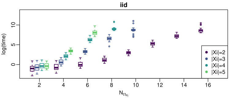
Figure 2: Boxplots of the logarithm of the computational time with different dimensions of the parent set $N_{\Pi_{X_{i}}}$ and number of states $|X_{i}|$, with parameters sampled with the hierarchical (top panel) or i.i.d (bottom panel) approach.

Figure 2 shows how the logarithm of the computational time varies as a function of the dimension of the parent set $N_{\Pi_{X_{i}}}$ for different values of $|X_{i}|$. The logarithm of the computational time scales linearly in the dimension of the parent set for each value of $|X_{i}|$, with a slope that is proportional to the value $|X_{i}|$. A deviation from this behaviour is visible for small values of $N_{\Pi_{X_{i}}}$ in the iid case, where the time needed to estimate the parameters is negligible compared to fixed computational costs like memory allocation.

The effect of $|F|$ on the computational times is weaker than that of $N_{\Pi_{X_{i}}}$ and $|X_{i}|$, while the effect of the number of observations $n_{f}$ is negligible.

To estimate the effect of $N_{\Pi_{X_{i}}}$, $|X_{i}|$ and $|F|$ on the computational time, we estimated the parameters of the linear model

$$\log(\text{Time})=\beta_{0}+\beta_{1}\mathbb{I}_{\text{iid}}+\beta_{2}\log(|F|)+\beta_{3}(1+N_{\Pi_{X_{i}}})\log(|X_{i}|)+\epsilon,$$

corresponding to

$$\text{Time}=e^{\beta_{0}+\beta_{1}\mathbb{I}_{\text{iid}}}|F|^{\beta_{2}}|X_{i}|^{\beta_{3}\left(1+N_{\Pi_{X_{i}}}\right)}e^{\epsilon},$$

where $\epsilon$ represents the measurement error. All the parameter estimates are significantly different from zero (the associated p-values are smaller than $10^{-15}$) and the model fits the computational times well ($R^{2}=0.95$). Moreover, the estimated parameters $\beta_{0}=-6.20$, $\beta_{1}=-0.84$, $\beta_{2}=0.71$ and $\beta_{3}=1.15$ are consistent with the theoretical computational complexity derived in (11).

5 Numerical example

We consider a simple example to illustrate the steps involved in learning a network structure with BHD and in estimating the associated parameters.

We consider in this example the set of variables $X_{1},\ldots,X_{5}$, with $|X_{i}|=2$ for $i=1,\ldots 5$, and $|F|=2$ related data sets. We assume that the true underlying structure for both the related data sets is that shown in the top panel of Figure 3, and that the parameters for the two related data sets are those summarised in Tables 5-6 in B. These parameters have been sampled from a hierarchical Dirichlet distribution with imaginary sample size equal to $10$ and with a parameter $\boldsymbol{\alpha}$ that is sampled from a Dirichlet distribution with all $\alpha_{0,ijk}=1$.

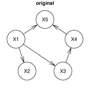
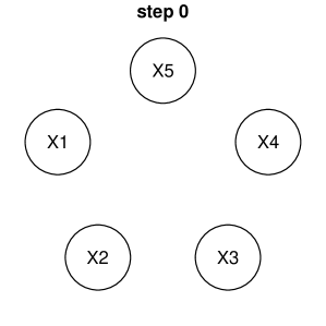
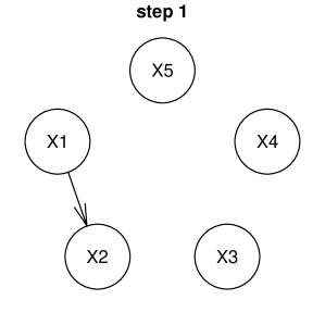
Figure 3: Original underlying network (top central panel) and networks estimated by means of BHD score during the 5 hill-climbing steps.

We learn the structure from $|F|$ related data sets, each containing $n_{f}=1000$ observations sampled from the true underlying distribution, with the hill-climbing implementation in bnlearn [27] with the BHD score with imaginary sample $s=1$.

Table 1: Scores associated with each node and overall score obtained in the numerical example hill-climbing optimisation. Step 0 corresponds to the starting empty graph, step 5 corresponds to the estimated network. The scores updated at each step due to arc addition are highlighted in bold.

step	$\mathbf{X_{1}}$	$\mathbf{X_{2}}$	$\mathbf{X_{3}}$	$\mathbf{X_{4}}$	$\mathbf{X_{5}}$	overall
0	-466.205	-528.450	-695.655	-642.506	-672.477	-3005.293
1	-466.205	-463.584	-695.655	-642.506	-672.477	-2940.427
2	-466.205	-463.584	-651.734	-642.506	-672.477	-2896.506
3	-466.205	-463.584	-651.734	-642.506	-666.052	-2890.081
4	-466.205	-463.584	-651.734	-642.506	-650.698	-2874.727
5	-466.205	-463.584	-651.734	-638.011	-650.698	-2870.232

The true underlying network is recovered after five optimisation steps, shown in Figure 3. The scores associated with each node and the increasing overall score obtained during the 5 steps of hill-climbing are summarised in Table 1. Tables 5-6 show the parameters estimated by means of the method described in [16], associated with the estimated network. The average absolute error in parameter estimation is $0.023$. The average absolute error decreases to $0.005$ when the number of observations increases to $n_{f}=10000$, thus showing the consistency of both the BHD score and the parameter estimation method as the size of the data set increases. In contrast, even with $n_{f}=10000$ both BDeu and BIC are unable to learn the true underlying network from the pooled data sets due to the differences between their distributions. Notice, e.g., the parameters associated to the node $X_{2}$ summarised in Table 5, which represent different associations between $X_{1}$ and $X_{2}$ across the two data sets. BHD is able to take into account different associations across data sets and to properly estimate the associated parameters (see Table 5). Both BDeu and BIC estimate instead no association between $X_{1}$ and $X_{2}$ because they pool the two data sets.

5.1 Sensitivity to the hyperparameters

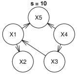
Figure 4: Networks estimated by means of BHD score with $s\in\{0.1,0.5,1,10,100\}$ and $s_{0}=1$. For a given value of $s$, the estimated network does not change as $s_{0}$ varies.

We repeat the experiment for different values of the hyperparameters $s$ and $s_{0}$ in the set $\{0.1,0.5,1,10,100\}$. The results are summarised in Figure 4. As $s$ increases the learned networks become more connected, similarly to what usually happens with BDeu (see [28] for a more detailed discussion). However, given a value of $s$, the same graph is learned for all the values of $s_{0}$. In future works, it may be interesting to further study how to choose a suitable value for $s$ for the BHD score or to model it as an hidden random variable with its own prior distribution.

6 Simulation Studies

We now perform some simulation studies to compare the empirical performance of BHD to that of BDeu and BIC. For brevity, we will not discuss the results for BIC in detail since they are fundamentally the same as those for BDeu. We are interested in structure learning in the following two scenarios:

1. the true underlying network is the same for all the related data sets;

2. the true underlying network is the same for all the related data sets, apart from $N_{F}$ data sets in which $N_{A}$ randomly selected arcs have been removed.

For each scenario, we generate synthetic data following three different models for the local distributions of each node:

1. the parameters associated with each of the related data sets are sampled from a hierarchical Dirichlet distribution with imaginary sample size equal to 10 and with a parameter $\boldsymbol{\alpha}_{i}$ sampled from a Dirichlet distribution with all $\alpha_{0,ijk}=1$;

2. the parameters associated with each of the related data sets are independently sampled from the same Dirichlet distribution with imaginary sample size equal to 10 and uniform $\boldsymbol{\alpha}_{i}$ vector;

3. the parameters are identical for all data sets.

The first approach follows the distributional assumptions of the hierarchical model underlying BHD and may favour the proposed score. The last approach may favour methods that do not take into account that data may comprise related data sets, thus pooling all the data and assuming that all observations are generated from the same distribution. The second approach is a middle ground between the first and the third, since parameters associated with the related data sets are different but they are not generated from the hierarchical model.

We then perform structure learning on the simulated data using the hill-climbing implementation in bnlearn [27] with the BHD and BDeu scores, both with imaginary sample $s=1$. In the case of BDeu we pool all the available data from different related data sets. We evaluate the accuracy of network reconstruction with the Structural Hamming Distance (SHD) [29] between the estimated and the true underlying structure, True Positive (TP), False Positive (FP) and False Negative (FN) arcs.

6.1 Simulation study 1

The aim of this simulation study is to evaluate the performance of BHD as different networks parameters vary. Specifically, we consider different number of nodes, related data sets and states for each variable.

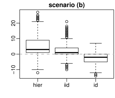
Figure 5: Simulation study 1: Boxplots of SHD difference between BHD and BDeu score for scenario (a) (left panel) and (b) (right panel). Positive values favour the hierarchical score.

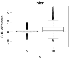
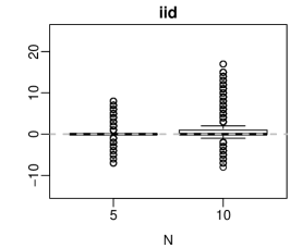
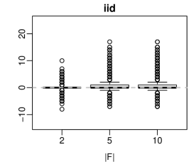
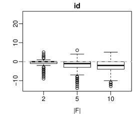
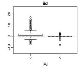
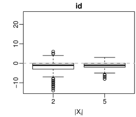
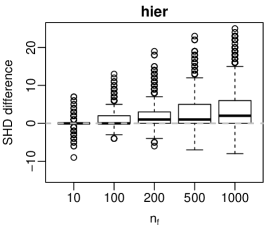
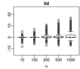
Figure 6: Simulation study 1: Boxplots of SHD difference between BHD and BDeu score for scenario (a) (equal structures) with different values of number of variables $N$, number of related data sets $|F|$, number of states $|X_{i}|$ and number of observations $n_{f}$, with parameters sampled with the hierarchical (left panels), i.i.d (central panels) or identical distribution (right panels) approach. Positive values favour the hierarchical score.

We first sample 3 network structures for each of three different levels of sparsity, such that they contain $\{1,1.2,1.5\}\cdot N$ arcs, and each combination of:

• $N\in\left\{5,10\right\}$, where $N$ represents the number of nodes;

• $|F|\in\left\{2,5,10\right\}$, where $|F|$ represents the number of related data sets;

• $|X_{i}|\in\left\{2,5\right\}$, where $|X_{i}|$ represents the number of states for each variable.

Then, for both scenario (a) and (b), we replicate the same structure for all the $|F|$ related data sets. In scenario (b), for each of the $N_{F}$ data sets differing from the others, we randomly remove $N_{A}$ arcs from the network, with $N_{F}\in\{1,2\}$ and $N_{A}\in\{1,2\}$. Thus, in scenario (b) we deal with $N_{F}$ structures that differ from one another and from the main structure by $N_{A}$ arcs.

Once the network structures have been generated, we sample 10 different parameter sets for each of hier, iid and id. Then, for each of these parameter sets, we sample $|F|$ related data sets, each containing $n_{f}\in\{10,100,200,500,1000\}$ observations.

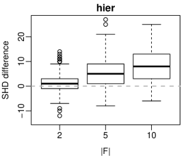
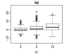
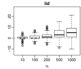
Figure 7: Simulation study 1: Boxplots of SHD difference between BHD and BDeu score for scenario (b) (different structures) with different values of number of related data sets $|F|$ and number of observations $n_{f}$, with parameters sampled with the hierarchical (left panels), i.i.d (central panels) or identical distribution (right panels) approach. Positive values favour the hierarchical score.

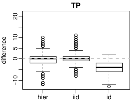
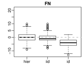
Figure 8: Simulation study 1: Boxplots of TP (left panel), FP (central panel) and FN (right panel) difference between BHD and BDeu score for scenario (b) (different structures). Positive values always favour the hierarchical score.

The difference between BDeu and BHD in terms of SHD for scenarios (a) and (b) is shown in Figure 5, respectively in the left and right panel. Positive values favour the proposed BHD score. When parameters are sampled from a hierarchical distribution (hier), BHD outperforms BDeu in both scenarios, with a larger improvement in scenario (b). In the iid case, BHD is competitive with BDeu when the underlying network structures are homogeneous, and it outperforms BDeu when the underlying network structures are different. On the other hand, in the id case BDeu has better accuracy than BHD because it correctly assumes that all the data are generated form the same distribution, while BHD has a large number of redundant parameters that would model the non-existing related data sets.

Figure 6 shows how the difference in SHD between BHD and BDeu varies for different simulation parameters in scenario (a). Specifically, the differences between BHD and BDeu (positive for hier and iid, negative for id) become increasingly large in magnitude as the number of variables $N$ or the number of related data sets $|F|$ increase. On the other hand, the differences between BHD and BDeu gradually decrease as the number of states $|X_{i}|$ increases. As for the sample size, BHD increasingly outperforms BDeu in both hier and iid as $n_{f}$ increases. In the id case we expect the two scores to be asymptotically equivalent, but the values we consider for $n_{f}$ are not large enough to clearly show it empirically.

Figure 7 shows the relationship between the difference in SHD and some key simulation parameters in scenario (b). The effect of both the number of related data sets $|F|$ and the number of observations $n_{f}$ is more marked than in scenario (a). For the same $|F|$ and $n_{f}$, BHD outperforms BDeu by a larger margin when some network structures are different (scenario (b)) compared to when they are all identical (scenario (a)).

Figure 8 shows the difference in TP (left), FP (center) and FN (right panel) between BDeu and BHD for scenario (b). Positive values favour the proposed BHD score. While the two methods perform similarly in terms of TP and FN, BHD outperforms BDeu in terms of FP in the hier case. The structures learned by BHD are thus sparser and more interpretable than those learned by BDeu.

We also perform some experiments with different values $s\in\{1,2,5,10\}$ of the imaginary sample size. As $s$ increases, BHD achieves marginally lower SHDs. However, its average SHD is not significantly different from that of BDeu for the same value of $s$.

6.2 Simulation study 2

Given the results of the first simulation study, we now focus on the effect of specific parameters on the performance of BHD. In particular, the aim of this simulation study is to evaluate the behaviour of the proposed score as the number of related data sets increases.

Similarly to the first simulation study, we sample one network structure for each of three different levels of sparsity ($\{1,1.2,1.5\}\cdot N$ arcs as before) and each of $|F|\in\left\{2,5,10,25,50,100\right\}$ related data sets. We treat both the number of nodes ($N=10$) and the number of states for each variable ($|X_{i}|=2$) as fixed.

Then, for both scenario (a) and (b), we replicate the same structure for all the $|F|$ related data sets. In scenario (b), for each of the $N_{F}$ data sets differing from the others, we randomly remove $N_{A}$ arcs from the network, with $N_{F}\in\{1,2,|F|\}$ and $N_{A}\sim\text{Bin}(N_{T},p)$, where $N_{T}$ is the total number of arcs and $p\in\{0.01,0.1\}$. Thus, in scenario (b) we deal with $N_{F}$ structures that differ from one another and from the main structure by $N_{A}$ arcs.

Once the network structures have been generated, we sample 10 different parameter sets for each structure and for each of hier and iid; for each of these parameter sets, we sample $|F|$ related data sets composed of $n_{f}\in\{10,100,200,500,1000,2000,$ $5000,10000\}$ observations each. In this simulation study we disregard the id case and we focus instead on the more interesting hier and iid cases.

Figures 9 and 10 show how the SHD difference between BHD and BDeu varies as the number of related data sets $|F|$ and the number of observations $n_{f}$ increase. Results obtained in scenario (a) and (b) are presented together for brevity. Moreover, we did not notice any practical difference as the number of removed arcs $N_{A}$ or the number of networks with a reduced number of arcs $N_{F}$ vary.

For small values of $|F|$ the improvement of BHD with respect to BDeu increases with $|F|$, while for large values of $|F|$ the difference between BHD and BDeu reaches a plateau. As expected, the gain is much larger in hier. In both hier and iid BHD increasingly outperforms BDeu as $n_{f}$ increases. The difference between the two scores is particularly clear for large values of $n_{f}$.

Figure 9: Simulation study 2: Boxplots of SHD difference between BHD and BDeu score with different values of number of related data sets $|F|$, with parameters sampled with the hierarchical (left panel) or i.i.d (right panel) approach. Positive values favour the hierarchical score.

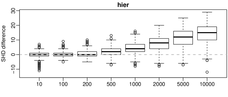
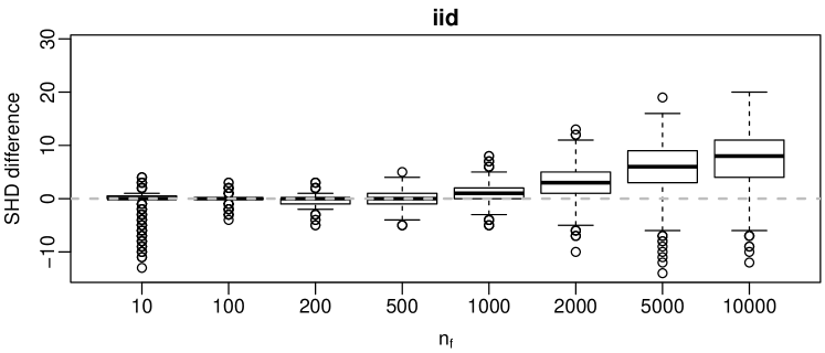
Figure 10: Simulation study 2: Boxplots of SHD difference between BHD and BDeu score with different values of number of observations $n_{f}$, with parameters sampled with the hierarchical (top panel) or i.i.d (bottom panel) approach. Positive values favour the hierarchical score.

The improvement of BHD with respect to BDeu in terms of SHD is the result of a lower number of FP arcs, as in the first simulation study. However, in this study BHD outperforms BDeu also in terms of TP and FN for large values of $n_{f}$.

6.3 Simulation study 3

Following up from the second simulation study, we now evaluate the performance of BHD as the number of nodes varies.

We sample a network structure for each of three different levels of sparsity (the same as in the first two studies) and each of $N\in\left\{5,10,25,50,100\right\}$ nodes. We treat the number of related data sets ($|F|=10$) and the number of states for each variable ($|X_{i}|=2$) as fixed.

The simulations are performed following the same steps as in the previous simulation study. For both scenario (a) and (b), we replicate the same structure for all the $|F|$ related data sets. We then we randomly remove $N_{A}$ arcs from the networks for each of the $N_{F}$ data sets differing from the others, as in simulation study 2; then we sample 10 parameter sets and, for each of them, $|F|$ related data sets with $n_{f}\in\{10,100,200,$ $500,1000,2000,$ $5000,10000\}$ observations.

Figure 11 shows the SHD difference between BHD and BDeu as a function of the number of nodes $N$. Results obtained in scenario (a) and (b) are presented together for brevity as in simulation study 2. The boxplots show that the bigger the number of nodes $N$, the larger the improvement of BHD with respect to BDeu. As expected, the gain is much larger in hier compared to iid for the same $N$.

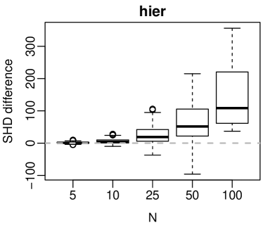
Figure 11: Simulation study 3: Boxplots of SHD difference between BHD and BDeu score with different values of number of variables $N$, with parameters sampled with the hierarchical (left panel) or i.i.d (right panel) approach. Positive values favour the hierarchical score.

As in the previous simulation study, the improvement of BHD with respect to BDeu can be attributed to a lower number of FP arcs. However, in this simulation study BHD outperforms BDeu also in terms of TP and FN for large values of $N$.

6.4 Simulation study 4

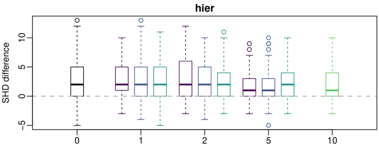
Figure 12: Simulation study 4: Boxplots of SHD difference between BHD and BDeu score with different number of sub-sampled data sets $N_{F}$ and proportions of sub-sampling $p$, with parameters sampled with the hierarchical (top panel) or i.i.d (bottom panel) approach. $N_{F}=0$ corresponds to the case where all the data sets have the same number of observations, $N_{F}=10$ corresponds to the case where the samples have dimensions $(0.25n_{f},0.25n_{f},0.5n_{f},0.5n_{f},0.75n_{f},0.75n_{f},0.75n_{f},n_{f},n_{f},n_{f})$ . Positive values favour the hierarchical score.

The aim of this simulation study is to evaluate the performance of BHD when each related data set is composed by a different number of observations. The simulation proceeds as in the previous studies, while treating the number of related data sets ($|F|=10$), the number of nodes ($N=10$) and the number of states for each variable ($|X_{i}|=2$) as fixed.

Only for scenario (a), we replicate the same structure for all the $|F|$ related data sets, we sample 10 different parameter sets for each structure and for each of hier and iid. Then, for each of these parameter sets, we sample $|F|$ related data sets, each of them composed of a number of observations $n_{f}\in\{100,500,1000\}$ which is the same for all the $|F|$ related data sets apart from $N_{F}$ data sets that are reduced to $p\cdot n_{f}$ observations, where $p\in\{0.1,0.25,0.5\}$.

Furthermore, we consider an additional case with a different number of observations for each related data set. Specifically we consider for the 10 related data sets a number of samples equal to $(0.25n_{f},0.25n_{f},0.5n_{f},0.5n_{f},0.75n_{f},0.75n_{f},0.75n_{f},$ $n_{f},n_{f},n_{f})$. This composite case will be identified by means of $N_{F}=10$. We compare all these cases using the standard case where all the related data sets are composed by the same number of observations $n_{f}$ as a baseline. This case will be identified by means of $N_{F}=0$.

Figure 12 shows the SHD difference between BHD and BDeu for different values of $N_{F}$ and $p$. The performance of BHD in all the sub-sampled scenarios is similar to the standard case ($N_{F}=0$). Also in the composite scenario, with a different number of observations for each related data set ($N_{F}=10$), the performance of BHD do not decrease significantly with respect to the equal-number-of-observation scenario. Analogously to the previous simulation studies, the gain is much larger in hier.

7 Conclusions and future work

In this work we propose a new Bayesian score, BHD, to learn a common BN structure from related data sets. BHD assumes that their joint distribution in each node of the network follows a mixture of Dirichlet distributions, thus pooling information between the data sets. The joint distribution in each node is approximated by means of a variational method. We found that the resulting computational complexity is linear in the number of related data sets, and that otherwise it is in the same class as BDeu. We showed with a comprehensive set of simulation studies that BHD outperforms both BDeu and BIC when applied to data that comprise related data sets; and that it has comparable performance to BDeu and BIC when the data are a single, homogeneous set of observations. Moreover, the larger is the number of the nodes in the network or the larger is the number of observations, the larger is the improvement with respect to both BDeu and BIC.

Learning a common BN structure with BHD builds on and complements our previous work on parameter learning from related data sets, described in [16]. We can use the latter to learn the parameters associated with a network structure learned using BHD, thus obtaining different BNs (one for each related data set) with the same structure and related parameters, as shown in the numerical example. Combining the two approaches may increase the performance of the BN models such as BN classifiers when dealing with related data sets. Future applications of the combined approach include, e.g., meta-analysis studies, which aim at combining information from several data sources [10, Sec. 5.6].

The assumptions underlying BHD can be relaxed in several ways to extend its applicability to more complex scenarios. For instance, relaxing the assumption that related data sets share the same dependence structure may allow to detect independencies that hold only in certain contexts, as in [30]. Such context-specific independences would be directly modelled by learning different but related network structures for each data set. Another interesting development would be to derive a conditional independence test from BHD to learn BNs from related data sets with constraint-based algorithm similarly to, e.g., [31].

Appendix A Estimation of variational parameters

For each node $X_{i}$, with $i=1,\ldots,N$, we estimate the variational parameters of model (8) by maximising a lower bound of the evidence lower bound (ELBO) for the marginal log-likelihood for the node $X_{i}$. The derivation of the bound and the algorithm used to estimate the variational parameters are described in detail in [16]. Here we summarise the parameter estimation method in Algorithm 1 and we adapt it to match the notation used in this paper.

Algorithm 1 Variational Estimator

For each $i=1,\ldots,N$, while $\text{iter}_{1}<m_{1}$ and $\mathit{tol_{1}}>t_{1}$:

1. Update $\widehat{\boldsymbol{\nu}}_{i}$ by means of (12)

2. Fix the starting values of $\widehat{\tau}_{i}$, $\widehat{\boldsymbol{\kappa}}_{i}$.

3. While $\text{iter}_{2}<m_{2}$ and $\mathit{tol_{2}}>t_{2}$:

   1. update $\widehat{\tau}_{i}$ given $\widehat{\boldsymbol{\kappa}}_{i}$ and $\widehat{\boldsymbol{\nu}}_{i}$ by means of (13);

   2. update $\widehat{\boldsymbol{\kappa}}_{i}$ given $\widehat{\tau}_{i}$ and $\widehat{\boldsymbol{\nu}}_{i}$ by means of (14);

   3. increase the iterator $\text{iter}_{2}$.

4. Update $\widehat{\tau}_{i}$, $\widehat{\boldsymbol{\kappa}}_{i}$ with the values estimated at the end of step 3.

5. Increase the iterator $\text{iter}_{1}$.

The lower bound of the ELBO for the node $X_{i}$ is the the functional ${\mathcal{L}}_{i}$, which is defined as

$${\mathcal{L}}_{i}= \sum_{f=1}^{|F|}\sum_{k=1}^{|X_{i}|}\sum_{j=1}^{|\Pi_{X_{i}}|}(n_{ijk}^{f}-\nu_{ijk}^{f}+s_{i}\kappa_{ijk})(\psi(\nu_{ijk}^{f})-\psi(\nu_{i\cdot\cdot}^{f}))+$$

$$+\sum_{f=1}^{|F|}\sum_{k=1}^{|X_{i}|}\sum_{j=1}^{|\Pi_{X_{i}}|}\log\Gamma(\nu_{ijk}^{f})-|F|\sum_{k=1}^{|X_{i}|}\sum_{j=1}^{|\Pi_{X_{i}}|}\log\Gamma(s_{i}\kappa_{ijk})+$$

$$+|F|\sum_{k=1}^{|X_{i}|}\sum_{j=1}^{|\Pi_{X_{i}}|}(s_{i}\kappa_{ijk}-1)(\log(\kappa_{ijk})-\psi(\tau_{i}\kappa_{ijk})+\psi(\tau_{i}))+$$

$$+\sum_{k=1}^{|X_{i}|}\sum_{j=1}^{|\Pi_{X_{i}}|}([\boldsymbol{\alpha}_{0}]_{ijk}-\tau_{i}\kappa_{ijk})(\psi(\tau_{i}\kappa_{ijk})-\psi(\tau_{i}))+$$

$$+\sum_{k=1}^{|X_{i}|}\sum_{j=1}^{|\Pi_{X_{i}}|}\log\Gamma(\tau_{i}\kappa_{ijk})-\sum_{k=1}^{|X_{i}|}\sum_{j=1}^{|\Pi_{X_{i}}|}\log\Gamma([\boldsymbol{\alpha}_{0}]_{ijk})-\sum_{f=1}^{|F|}\log\Gamma(\nu_{i\cdot\cdot}^{f})+$$

$$+|F|\log\Gamma(s_{i})-\frac{s_{i}}{\tau_{i}}|F|\left(|X_{i}||\Pi_{X_{i}}|-1\right)+\log\Gamma\left(s_{0}\right)-\log\Gamma(\tau_{i}),$$

where $\nu_{i\cdot\cdot}^{f}=\sum_{k=1}^{|X_{i}|}\sum_{j=1}^{|\Pi_{X_{i}}|}\nu_{ijk}^{f}$ and $\psi(\cdot)$ is the digamma function, the derivative of the $\log\Gamma(\cdot)$ function.

For each data set $F=f$, with $f=1,\ldots,|F|$, we can first estimate the quantity $\nu_{ijk}^{f}$, associated with the configuration $k$ of $X_{i}$ and $j$ of $\Pi_{X_{i}}$, by maximising $\mathcal{L}_{i}$ with respect to $\nu_{ijk}^{f}$ and by assuming $\kappa_{ijk}$ to be fixed. By setting the partial derivative of $\mathcal{L}_{i}$ with respect to $\nu_{ijk}^{f}$ to zero, we obtain:

$$\hat{\nu}_{ijk}^{f}=n_{ijk}^{f}+s_{i}\kappa_{ijk}.$$ (12)

We can then estimate $\hat{\tau}_{i}$ and $\hat{\kappa}_{ijk}$ given the value of $\nu_{ijk}^{f}$ by means of a fixed-point method, which alternates the optimisation of $\mathcal{L}_{i}$ with respect to $\tau_{i}$ and $\kappa_{ijk}$. Since no analytical solution is available, we perform this optimisation by means of a Newton algorithm.

We obtain the Newton update for $\tau_{i}$ by treating $\boldsymbol{\kappa}_{i}$ as fixed to a vector whose elements are the quantities $\kappa_{ijk}$ with $j=1,\ldots,|\Pi_{X_{i}}|$ and $k=1,\ldots,|X_{i}|$. If we define

$$g_{\tau_{i}}(\tau_{i},\boldsymbol{\kappa}_{i})={\partial\mathcal{L}_{i}}/{\partial\tau_{i}}=\frac{s_{i}}{\tau_{i}^{2}}|F|\left(|X_{i}||\Pi_{X_{i}}|-1\right)+$$

$$+\sum_{k=1}^{|X_{i}|}\sum_{j=1}^{|\Pi_{X_{i}}|}(\psi^{\prime}(\tau_{i}\kappa_{ijk})\kappa_{ijk}-\psi^{\prime}(\tau_{i}))([\boldsymbol{\alpha}_{0}]_{ijk}-\tau_{i}\kappa_{ijk}-|F|(s_{i}\kappa_{ijk}-1))$$

and

$$h_{\tau_{i}}(\tau_{i},\boldsymbol{\kappa}_{i})={\partial^{2}\mathcal{L}_{i}}/{\partial\tau_{i}^{2}}=-\frac{2s_{i}}{\tau_{i}^{3}}|F|\left(|X_{i}||\Pi_{X_{i}}|-1\right)-\sum_{k=1}^{|X_{i}|}\sum_{j=1}^{|\Pi_{X_{i}}|}\psi^{\prime}(\tau_{i}\kappa_{ijk})\kappa^{2}_{ijk}+$$

$$+\psi^{\prime}(\tau_{i})+\sum_{k=1}^{|X_{i}|}\sum_{j=1}^{|\Pi_{X_{i}}|}(\psi^{\prime\prime}(\tau_{i}\kappa_{ijk})\kappa^{2}_{ijk}-\psi^{\prime\prime}(\tau_{i}))([\boldsymbol{\alpha}_{0}]_{ijk}-\tau_{i}\kappa_{ijk}-|F|(s_{i}\kappa_{ijk}-1)),$$

the Newton update for the parameter $\tau_{i}$ becomes

$$\hat{\tau}_{i}=\hat{\tau}^{\text{old}}_{i}\exp\left(-\frac{g_{\tau_{i}}(\hat{\tau}_{i}^{\text{old}},\boldsymbol{\kappa}_{i})}{h_{\tau_{i}}(\hat{\tau}_{i}^{\text{old}},\boldsymbol{\kappa}_{i})\hat{\tau}_{i}^{\text{old}}+g_{\tau_{i}}(\hat{\tau}_{i}^{\text{old}},\boldsymbol{\kappa}_{i})}\right),$$ (13)

where $\hat{\tau}_{i}^{\text{old}}$ is the estimate for $\tau_{i}$ in the previous iteration of the Newton algorithm.

We obtain the Newton update for the parameter vector $\boldsymbol{\kappa}_{i}$ by treating $\tau_{i}$ and $\boldsymbol{\nu}_{i}$ as fixed: their elements are the quantities $\nu_{ijk}^{f}$ with $f=1,\ldots,|F|$, $j=1,\ldots,|\Pi_{X_{i}}|$ and $k=1,\ldots,|X_{i}|$. If we define

$$g_{\kappa_{ijk}}(\boldsymbol{\kappa}_{i},\tau,\boldsymbol{\nu}_{i})={\partial\mathcal{L}_{i}}/{\partial\kappa_{ijk}}=\sum_{f=1}^{|F|}s_{i}(\psi(\nu_{ijk}^{f})-\psi(\nu_{i\cdot\cdot}^{f})+\tau_{i}\psi^{\prime}(\tau_{i}\kappa_{ijk})([\boldsymbol{\alpha}_{0}]_{ijk}+$$

$$-\tau_{i}\kappa_{ijk}-|F|(s_{i}\kappa_{ijk}-1))+\tau_{i}\psi(\tau_{i})+s_{i}|F|(\psi(\tau_{i})-\psi(\tau_{i}\kappa_{ijk})-\psi(s_{i}\kappa_{ijk})+$$

$$+\log(\kappa_{ijk})+1)-\frac{|F|}{\kappa_{ijk}}$$

and

$$h_{\kappa_{ijk}}(\boldsymbol{\kappa}_{i},\tau_{i},\boldsymbol{\nu}_{i})={\partial^{2}\mathcal{L}_{i}}/{\partial\kappa^{2}_{ijk}}=\tau_{i}^{2}\psi^{\prime\prime}(\tau_{i}\kappa_{ijk})([\boldsymbol{\alpha}_{0}]_{ijk}-\tau_{i}\kappa_{ijk}+$$

$$-|F|(s_{i}\kappa_{ijk}-1))-\tau_{i}\psi^{\prime}(\tau_{i}\kappa_{ijk})(\tau_{i}+2s_{i}|F|)-s_{i}^{2}|F|\psi^{\prime}(s_{i}\kappa_{ijk})+\frac{s_{i}|F|}{\kappa_{ijk}}+\frac{|F|}{\kappa^{2}_{ijk}},$$

we can write the Newton update for $\kappa_{ijk}$ as

$$\hat{\kappa}_{ijk}=\hat{\kappa}_{ijk}^{\text{old}}+\frac{\displaystyle{\sum_{l=1}^{|X_{i}|}\sum_{\jmath=1}^{|\Pi_{X_{i}}|}\frac{g_{\kappa_{i\jmath l}}(\boldsymbol{\kappa}_{i}^{\text{old}},\tau_{i},\boldsymbol{\nu}_{i})}{h_{\kappa_{i\jmath l}}(\boldsymbol{\kappa}_{i}^{\text{old}},\tau_{i},\boldsymbol{\nu}_{i})}}}{\displaystyle{\sum_{l=1}^{|X_{i}|}\sum_{\jmath=1}^{|\Pi_{X_{i}}|}\frac{h_{\kappa_{ijk}}(\boldsymbol{\kappa}_{i}^{\text{old}},\tau_{i},\boldsymbol{\nu}_{i})}{h_{\kappa_{i\jmath l}}(\boldsymbol{\kappa}_{i}^{\text{old}},\tau_{i},\boldsymbol{\nu}_{i})}}}-\frac{g_{\kappa_{ijk}}(\boldsymbol{\kappa}_{i}^{\text{old}},\tau_{i},\boldsymbol{\nu}_{i})}{h_{\kappa_{ijk}}(\boldsymbol{\kappa}_{i}^{\text{old}},\tau_{i},\boldsymbol{\nu}_{i})},$$ (14)

where $\kappa_{ijk}^{\text{old}}$ is the estimate for $\kappa_{ijk}$ in the previous iteration of the Newton algorithm.

Appendix B Parameters of numerical example

Tables 5-6 show the original and the estimated parameters of the network used in the numerical example presented in Section 5.

Table 2: Parameters associated with $X_{1}$.

	original		estimated
$X_{1}|F$	$1$	$2$	$1$	$2$
$1$	0.42	0.18	0.41	0.17
$2$	0.58	0.82	0.59	0.83

Table 3: Parameters associated with $X_{2}$.

	original				estimated
$F$	$1$		$2$		$1$		$2$
$X_{2}|X_{1}$	$1$	$2$	$1$	$2$	$1$	$2$	$1$	$2$
$1$	0.31	0.65	0.56	0.16	0.33	0.64	0.58	0.14
$2$	0.69	0.35	0.44	0.84	0.67	0.36	0.42	0.86

Table 4: Parameters associated with $X_{3}$.

	original				estimated
$F$	$1$		$2$		$1$		$2$
$X_{3}|X_{1}$	$1$	$2$	$1$	$2$	$1$	$2$	$1$	$2$
$1$	0.61	0.42	0.15	0.53	0.64	0.39	0.15	0.54
$2$	0.39	0.58	0.85	0.47	0.36	0.61	0.85	0.46

Table 5: Parameters associated with $X_{4}$.

	original				estimated
$F$	$1$		$2$		$1$		$2$
$X_{4}|X_{3}$	$1$	$2$	$1$	$2$	$1$	$2$	$1$	$2$
$1$	0.47	0.51	0.38	0.28	0.45	0.51	0.40	0.28
$2$	0.53	0.49	0.62	0.72	0.55	0.49	0.60	0.72

Table 6: Parameters associated with $X_{5}$.

	original
$F$	$1$				$2$
$X_{4}$	$1$		$2$		$1$		$2$
$X_{5}|X_{1}$	$1$	$2$	$1$	$2$	$1$	$2$	$1$	$2$
$1$	0.46	0.56	0.57	0.52	0.65	0.43	0.22	0.38
$2$	0.54	0.44	0.43	0.48	0.35	0.57	0.78	0.62
	estimated
$F$	$1$				$2$
$X_{4}$	$1$		$2$		$1$		$2$
$X_{5}|X_{1}$	$1$	$2$	$1$	$2$	$1$	$2$	$1$	$2$
$1$	0.41	0.58	0.53	0.53	0.77	0.44	0.14	0.38
$2$	0.59	0.42	0.47	0.47	0.23	0.56	0.86	0.62

Acknowledgements

We would like to acknowledge support for this project from the Swiss National Science Foundation (NSF, Grant No. IZKSZ2_162188).

References

- Gray [1994] R. J. Gray, A Bayesian Analysis of Institutional Effects in a Multicenter Cancer Clinical Trial, Biometrics 50 (1994) 244–253.
- Spiegelhalter et al. [2004] D. J. Spiegelhalter, K. R. Abrams, J. P. Myles, Bayesian Approaches to Clinical Trials and Health-Care Evaluation, Wiley, 2004.
- Goddard [2009] M. E. Goddard, Genomic Selection: Prediction of Accuracy and Maximisation of Long Term Response, Genetica 136 (2009) 245–257.
- Wientjes et al. [2016] Y. C. J. Wientjes, P. Bijma, R. F. Veerkamp, M. P. L. Calus, An Equation to Predict the Accuracy of Genomic Values by Combining Data from Multiple Traits, Populations, or Environments, Genetics 202 (2016) 799–823.
- Makowsky et al. [2011] R. Makowsky, N. M. Pajewski, Y. C. Klimentidis, A. I. Vazquez, C. W. Duarte, D. B. Allison, G. de los Campos, Beyond Missing Heritability: Prediction of Complex Traits, PLoS Genet. 7 (2011) e1002051.
- de los Campos et al. [2013] G. de los Campos, A. I. Vazquez, R. L. Fernando, Y. C. Klimentidis, D. Sorensen, Prediction of Complex Human Traits Using the Genomic Best Linear Unbiased Predictor, PLoS Genet. 9 (2013) e1003608.
- Russell et al. [2018] A. Russell, M. Ghalaieny, B. Gazdiyeva, S. Zhumabayeva, A. Kurmanbayeva, K. K. Akhmetov, Y. Mukanov, M. McCann, M. Ali, A. Tucker, C. Vitolo, A. Althonayan, A Spatial Survey of Environmental Indicators for Kazakhstan: An Examination of Current Conditions and Future Needs, International Journal of Environmental Research 12 (2018) 735–748.
- Vitolo et al. [2018] C. Vitolo, M. Scutari, A. Tucker, A. Russell, Modelling Air Pollution, Climate and Health Data Using Bayesian Networks: a Case Study of the English Regions, Earth and Space Science 5 (2018) 76–88.
- Qian et al. [2010] S. S. Qian, T. F. Cuffney, I. Alameddine, G. McMahon, K. H. Reckhow, On the Application of Multilevel Modeling in Environmental and Ecological studies, Ecology 91 (2010) 355–361.
- Gelman et al. [2014] A. Gelman, J. B. Carlin, H. S. Stern, D. B. Dunson, A. Vehtari, D. B. Rubin, Bayesian Data Analysis, 3rd ed., CRC press, 2014.
- Koller and Friedman [2009] D. Koller, N. Friedman, Probabilistic Graphical Models: Principles and Techniques, MIT press, 2009.
- Niculescu-Mizil and Caruana [2007] A. Niculescu-Mizil, R. Caruana, Inductive Transfer for Bayesian Network Structure Learning, in: Proceedings of Artificial Intelligence and Statistics, 2007, pp. 339–346.
- Oates et al. [2016] C. J. Oates, J. Q. Smith, S. Mukherjee, J. Cussens, Exact Estimation of Multiple Directed Acyclic Graphs, Statistics and Computing 26 (2016) 797–811.
- De Michelis et al. [2006] F. De Michelis, P. Magni, P. Piergiorgi, M. A. Rubin, R. Bellazzi, A Hierarchical Naive Bayes Model for Handling Sample Heterogeneity in Classification Problems: an Application to Tissue Microarrays, BMC bioinformatics 7 (2006) 514.
- Malovini et al. [2012] A. Malovini, N. Barbarini, R. Bellazzi, F. De Michelis, Hierarchical Naive Bayes for Genetic Association Studies, BMC bioinformatics 13 (2012) S6.
- Azzimonti et al. [2019] L. Azzimonti, G. Corani, M. Zaffalon, Hierarchical Estimation of Parameters in Bayesian Networks, Computational Statistics & Data Analysis 137 (2019) 67–91.
- Heckerman et al. [1995] D. Heckerman, D. Geiger, D. M. Chickering, Learning Bayesian Networks: The Combination of Knowledge and Statistical Data, Machine Learning 20 (1995) 197–243. Available as Technical Report MSR-TR-94-09.
- Lauritzen and Wermuth [1989] S. L. Lauritzen, N. Wermuth, Graphical Models for Associations Between Variables, Some of Which are Qualitative and Some Quantitative, The Annals of Statistics 17 (1989) 31–57.
- Schwarz [1978] G. Schwarz, Estimating the Dimension of a Model, The Annals of Statistics 6 (1978) 461–464.
- Ueno [2010] M. Ueno, Learning Networks Determined by the Ratio of Prior and Data, in: Proceedings of the 26th Conference on Uncertainty in Artificial Intelligence, 2010, pp. 598–605.
- Scutari [2016] M. Scutari, An Empirical-Bayes Score for Discrete Bayesian Networks, Journal of Machine Learning Research (Proceedings Track, PGM 2016) 52 (2016) 438–448.
- Scutari [2018] M. Scutari, Dirichlet Bayesian Network Scores and the Maximum Relative Entropy Principle, Behaviormetrika 45 (2018) 337–362.
- Chickering [1995] D. M. Chickering, A Transformational Characterization of Equivalent Bayesian Network Structures, in: Proceedings of the 11th Conference on Uncertainty in Artificial Intelligence, UAI ’95, 1995, pp. 87–98.
- Jordan et al. [1999] M. I. Jordan, Z. Ghahramani, T. S. Jaakkola, L. K. Saul, An Introduction to Variational Methods for Graphical Models, Machine Learning 37 (1999) 183–233.
- Wainwright and Jordan [2008] M. J. Wainwright, M. I. Jordan, Graphical Models, Exponential Families, and Variational Inference, Foundations and Trends in Machine Learning 1 (2008) 1–305.
- Casella and Moreno [2009] G. Casella, E. Moreno, Assessing Robustness of Intrinsic Tests of Independence in Two-Way Contingency Tables, Journal of the American Statistical Association 104 (2009) 1261–1271.
- Scutari [2010] M. Scutari, Learning Bayesian Networks with the bnlearn R Package, Journal of Statistical Software 35 (2010) 1–22.
- Silander et al. [2007] T. Silander, P. Kontkanen, P. Myllymäki, On sensitivity of the map bayesian network structure to the equivalent sample size parameter, in: Proceedings of the Twenty-Third Conference on Uncertainty in Artificial Intelligence, 2007, pp. 360–367.
- Tsamardinos et al. [2006] I. Tsamardinos, L. E. Brown, C. F. Aliferis, The Max-Min Hill-Climbing Bayesian Network Structure Learning Algorithm, Machine Learning 65 (2006) 31–78.
- Boutilier et al. [1996] C. Boutilier, N. Friedman, M. Goldszmidt, D. Koller, Context-Specific Independence in Bayesian Networks, in: Proceedings of the 12th International Conference on Uncertainty in Artificial Intelligence, UAI ’97, 1996, pp. 115–123.
- Tillman [2009] R. E. Tillman, Structure Learning with Independent Non-Identically Distributed Data, in: Proceedings of the 26th Annual International Conference on Machine Learning, ICML ’09, 2009, pp. 1041–1048.