Structural and Thermodynamic Properties of Hard-Sphere Fluids

Abstract

This Perspective article provides an overview of some of our analytical approaches to the computation of the structural and thermodynamic properties of single-component and multicomponent hard-sphere fluids. For the structural properties, they yield a thermodynamically consistent formulation, thus improving and extending the known analytical results of the Percus–Yevick theory. Approximate expressions linking the equation of state of the single-component fluid to the one of the multicomponent mixture are also discussed.

Nomenclature

Acronyms

BGHLL	Boublík–Grundke–Henderson–Lee–Levesque
BMCSL	Boublík–Mansoori–Carnahan–Starling–Leland
CS	Carnahan–Starling
DCF	direct correlation function
EOS	equation of state
FMT	fundamental measure theory
GMSA	generalized mean spherical approximation
HNC	hypernetted-chain
HS	hard sphere
LDH	linearized Debye–Hückel
MC	Monte Carlo
MD	molecular dynamics
MSA	mean spherical approximation
OZ	Ornstein–Zernike
PY	Percus–Yevick
RDF	radial distribution function
RFA	rational function approximation
SPT	scaled particle theory

I Introduction

It is widely recognized that a major breakthrough in the theory of liquids was provided by the notion (already put forward by van der Waals) that in a dense fluid, the repulsive forces are mostly responsible for its structure. It is also well known that in the statistical thermodynamic approach to such a theory, there is a close connection between the thermodynamic and structural properties.Barker and Henderson (1976); McQuarrie (1976); Friedman (1985); Hansen and McDonald (2006) In simple fluids, the radial distribution function (RDF) $g(r)$ (which describes the probability of finding a particle at a distance $r$ from another particle) and its close relative (through a Fourier transform), the static structure factor $S(q)$, are the basic quantities used to discuss the structural properties. The importance of $g(r)$ arises from the fact that, given the form of the potential of the intermolecular force (which is generally assumed to be well represented by pair interactions), the standard methods of statistical mechanics allow for the determination of all the equilibrium properties of the fluid, in particular its equation of state (EOS), if the RDF is known as a function of $r$, the number density $\rho$, and the temperature $T$.

The simplest repulsive model pair potential is that of a hard-core fluid (rods, disks, spheres, and hyperspheres) in which attractive forces are completely neglected. In fact, it is a model that has been most studied and has rendered some analytical results, although—up to this day—no general (exact) explicit expressions for the structural functions or the EOS are available, except in the one-dimensional case. An interesting feature concerning the thermodynamic properties of such model is that the EOS depends only on the contact values of the RDF. In the absence of a completely analytical approach, the most popular methods to deal with the properties of these systems are integral equation theories and computer simulations.

In real gases and liquids at high temperatures, the thermodynamic properties are also determined almost entirely by the repulsive forces among molecules. However, attractive forces become significant at lower temperatures. Nevertheless, even in this case, the attractive forces affect very little the configuration of the system at moderate and high densities. These facts are taken into account in the application of the perturbation theory of fluids,Solana (2013) where hard-core fluids are used as the reference systems in the computation of the thermodynamic and structural properties of real fluids. In any case, successful results using perturbation theory are rather limited because, as mentioned above, there are in general no exact (analytical) expressions for the thermodynamic and structural properties of the reference systems, which are, in principle, required in the calculations. On the other hand, in the realm of soft condensed matter, the use of the hard-sphere (HS) model in connection with sterically stabilized colloidal systems, is quite common. This reflects the fact that presently, it is possible to prepare (almost) monodisperse spherical colloidal particles with short-ranged harshly repulsive interparticle forces that may be well described theoretically with the HS potential.

This paper presents an overview of the efforts we have made over the years to compute the thermodynamic and structural properties of hard-core systems in $d$ dimensions using relatively simple (approximate) analytical methods. Due to their particular relevance and for the sake of concreteness, we will concentrate here on three-dimensional systems, namely, the HS fluid and the multicomponent HS fluid mixture. The paper is structured as follows. In Section II, we begin by recalling the main statistical–mechanical relationships, valid for general fluids, related to both their structural and thermodynamic properties, as well as some key approximate results derived for them in our systems of interest; special attention is paid to the thermodynamic routes and to a summary of results pertaining to the phase behavior of these systems, including some concerning the demixing transition. This is followed in Sec. III by a detailed account of an alternative methodology to the usual integral equation approach of liquid-state theory to obtain analytical results for the structural properties of HS fluids and multicomponent HS mixtures. Section IV is devoted to describe the routes we have followed to derive the EOS of a multicomponent HS mixture once the EOS of the monocomponent HS fluid is known, which allows one, in principle, to probe the metastable fluid branch of the single-component fluid. The paper is closed in Sec. V with some concluding remarks.

II Statistical mechanics, thermodynamics, and structure of fluids

II.1 General background

II.1.1 One-component systems

We begin with the partition function $\mathcal{Z}_{N}(\beta_{T},V)$ in the canonical ensemble for a closed system of $N$ identical particles of mass $m$ enclosed in a volume $V$ at a temperature $T$ (with $\beta_{T}\equiv{1}/{k_{B}T}$, $k_{B}$ being the Boltzmann constant), namely,

$$\mathcal{Z}_{N}(\beta_{T},V)=\frac{1}{N!h^{3N}}\int d\mathbf{x}^{N}\,e^{-\beta_{T}H_{N}(\mathbf{x}^{N})},$$ (1)

where $h$ is the Planck constant, $H_{N}(\mathbf{x}^{N})$ the Hamiltonian of the system, $\mathbf{x}^{N}\equiv\{\mathbf{r}^{N},\mathbf{p}^{N}\}$, $d\mathbf{x}^{N}\equiv d\mathbf{r}^{N}d\mathbf{p}^{N}$, $\mathbf{r}^{N}=\{\mathbf{r}_{1},\mathbf{r}_{2},\ldots,\mathbf{r}_{N}\}$, $d\mathbf{r}^{N}\equiv d\mathbf{r}_{1}d\mathbf{r}_{2}\cdots d\mathbf{r}_{N}$, $\mathbf{p}^{N}\equiv\{\mathbf{p}_{1},\mathbf{p}_{2},\ldots,\mathbf{p}_{N}\}$, and $d\mathbf{p}^{N}\equiv d\mathbf{p}_{1}d\mathbf{p}_{2}\cdots d\mathbf{p}_{N}$ (with $\mathbf{r}_{\alpha}$ and $\mathbf{p}_{\alpha}$, $\alpha=1,2,\ldots,N$, denoting the position and momentum vectors of particle $\alpha$, respectively). In the general case of interacting particles, the Hamiltonian is given by $H_{N}(\mathbf{x}^{N})=H_{N}^{\text{id}}(\mathbf{p}^{N})+\Phi_{N}(\mathbf{r}^{N})$, where $H_{N}^{\text{id}}(\mathbf{p}^{N})=\sum_{\alpha=1}^{N}{p_{\alpha}^{2}}/{2m}$ accounts for the kinetic energy of the particles and $\Phi_{N}(\mathbf{r}^{N})$ is the intermolecular potential. Hence, one may rewrite the partition function as $\mathcal{Z}_{N}(\beta_{T},V)=\mathcal{Z}_{N}^{\text{id}}(\beta_{T},V)\mathcal{Q}_{N}(\beta_{T},V)$, where $\mathcal{Z}_{N}^{\text{id}}(\beta_{T},V)={V^{N}}/{N!\Lambda^{3N}}$, $\Lambda=h\sqrt{{\beta_{T}}/{2\pi m}}$ being the thermal de Broglie wavelength, and $\mathcal{Q}_{N}(\beta_{T},V)=V^{-N}\int d\mathbf{r}^{N}\,e^{-\beta_{T}\Phi_{N}(\mathbf{r}^{N})}$ is the configuration integral.

Given the fact that the partition function and the Helmholtz free energy of the system are linked by $F(N,V,T)=-\beta_{T}^{-1}\ln\mathcal{Z}_{N}(\beta_{T},V)$, and since the average energy, the pressure, the isothermal compressibility, and the chemical potential of the fluid are obtained from the Helmholtz free energy as

$$\langle E\rangle=\frac{\partial(\beta_{T}F)}{\partial\beta_{T}},$$ (2a)

$$p=-\frac{\partial F}{\partial V},$$ (2b)

$$\kappa_{T}^{-1}\equiv-V\frac{\partial p}{\partial V}=V\frac{\partial^{2}F}{\partial V^{2}},$$ (2c)

$$\mu=\frac{\partial F}{\partial N},$$ (2d)

respectively, in order to derive such thermodynamic properties all that one, in principle, needs is the explicit form of $\Phi_{N}(\mathbf{r}^{N})$ and the subsequent computation of the configuration integral. However, in practical terms, dealing with an $N$-particle problem when $N\sim 10^{23}$ is not, in general, feasible. Nevertheless, one way to attempt to make it feasible is by reducing the problem of a macroscopic fluid in a volume $V$ to a sum of an increasing number of tractable isolated few ($n=1$, $2$, $3$, …) particle problems, where each group of particles moves alone in the volume $V$ of the system. In the case of the pressure, this approach leads formally to the virial expansion of the EOS, which reads

$$\beta_{T}p(\rho,T)=\rho+\sum_{n=2}^{\infty}B_{n}(T)\rho^{n},$$ (3)

where $\rho=N/V$ is the number density. Such an expansion was introduced empirically by ThiesenThiesen (1885) and (independently) by Kamerlingh OnnesKamerlingh Onnes (1901) with the aim of providing a mathematical representation of experimental results of the dependence of pressure on temperature and density of gases and liquids through an expansion of the pressure in powers of density. In fact, it was Kamerlingh Onnes who named the coefficients $B_{n}(T)$ in the expansion the virial coefficients. Once the statistical–mechanical rigorous derivation of this series became available, it was immediate to relate the virial coefficients to intermolecular interactions involving $n$ particles. Such relationships, derived originally by Mayer and Mayer,Mayer and Goeppert Mayer (1940) imply that the $n$th virial coefficient can be written as a sum of integrals represented by the so-called $n$-particle star graphs. It is unfortunate, however, that—in general—the actual computation of the virial coefficients is a formidable task, and that the radius of convergence of the series in Eq. (3) is not known. Nevertheles, if $\rho$ is small enough and if the required first few virial coefficients are available, a reasonable approximation to the EOS of the system may thus be derived. We will come back to this point later on for the specific case of HS fluids and fluid mixtures. A review on virial expansions, including an extensive list of references and a description of the difficulties associated with the computation of higher virial coefficients, has been written by Masters.Masters (2008) In a rather recent paper, Hoover and HooverHoover and Hoover (2020) have provided a nice account on the early history of the numerical computation of virial coefficients and the more recent developments.

Now we turn to the structural properties. Although of course it is the full $N$-body probability distribution function $\varrho_{N}(\mathbf{x}^{N})$ that contains all the statistical–mechanical information about the system, marginal few-body distributions may be enough for the most relevant quantities. Let us now introduce the reduced $s$-body correlation functions $f_{s}(\mathbf{x}^{s})$ so that $f_{s}(\mathbf{x}^{s})d\mathbf{x}^{s}$ corresponds to the number of groups of $s$ particles such that one particle lies inside a volume $d\mathbf{x}_{1}$ around the (one-body) phase-space point $\mathbf{x}_{1}$, other particle lies inside a volume $d\mathbf{x}_{2}$ around the (one-body) phase-space point $\mathbf{x}_{2}$, …, and so on. Hence,

$$f_{s}(\mathbf{x}^{s})=\frac{N!}{(N-s)!}\int d\mathbf{x}_{s+1}\int d\mathbf{x}_{s+2}\cdots\int d\mathbf{x}_{N}\,\varrho_{N}(\mathbf{x}^{N}).$$ (4)

Since, in equilibrium, the momenta of all the particles are uncorrelated, it is also convenient to introduce the configurational $s$-body correlation functions $n_{s}(\mathbf{r}^{s})$ obtained by integrating $f_{s}(\mathbf{x}^{s})$ over the momenta. These correlation functions are translationally invariant. In the particular case $s=2$, $n_{2}(\mathbf{r}_{1},\mathbf{r}_{2})=\int d\mathbf{p}_{1}\int d\mathbf{p}_{2}\,f_{2}(\mathbf{x}_{1},\mathbf{x}_{2})$, and it follows from the constant number of particles that $\int d\mathbf{r}_{1}\int d\mathbf{r}_{2}\,n_{2}(\mathbf{r}_{1},\mathbf{r}_{2})=N(N-1)$.

Recalling that in the canonical ensemble $\varrho_{N}(\mathbf{x}^{N})$ is given by

$$\varrho_{N}(\mathbf{x}^{N})=\frac{e^{-\beta_{T}H_{N}(\mathbf{x}^{N})}}{N!h^{3N}\mathcal{Z}_{N}^{\text{id}}\mathcal{Q}_{N}},$$ (5)

one has

$$n_{2}(\mathbf{r}_{1},\mathbf{r}_{2})=\frac{N(N-1)}{V^{N}\mathcal{Q}_{N}}\int d\mathbf{r}_{3}\cdots\int d\mathbf{r}_{N}\,e^{-\beta_{T}\Phi_{N}(\mathbf{r}^{N})}.$$ (6)

In turn, defining the pair correlation function $g_{2}(\mathbf{r}_{1},\mathbf{r}_{2})$ by $n_{2}(\mathbf{r}_{1},\mathbf{r}_{2})=\rho^{2}{g_{2}(\mathbf{r}_{1},\mathbf{r}_{2})}$, one obtains

$$g_{2}(\mathbf{r}_{1},\mathbf{r}_{2})=\frac{V^{-(N-2)}}{\mathcal{Q}_{N}}\int d\mathbf{r}_{3}\cdots\int d\mathbf{r}_{N}\,e^{-\beta_{T}\Phi_{N}(\mathbf{r}^{N})},$$ (7)

where we have taken into account that $N-1\approx N$.

A fluid is also rotationally invariant. Therefore, assuming central forces and using translational invariance, it follows that $g_{2}(\mathbf{r}_{1},\mathbf{r}_{2})=g_{2}(\mathbf{r}_{1}-\mathbf{r}_{2})=g(r)$ with $r\equiv|\mathbf{r}_{1}-\mathbf{r}_{2}|$, so that this pair correlation function is precisely the RDF. Note that, once again, knowledge of the intermolecular potential would be, in principle, enough to obtain $g(r)$. Also note that, if a given particle is taken to be at the origin, then the local average density at a distance $r$ from that particle is $\rho g(r)$. Therefore, as already mentioned, $g(r)$ is a measure of the probability of finding a particle at a distance $r$ away from a given reference particle, relative to that for an ideal gas.

Other important related structural quantities are the total correlation function $h(r)\equiv g(r)-1$, the static structure factor

$$S(q)=1+\rho\int d\mathbf{r}\,h(r)e^{-\imath\mathbf{q}\cdot\mathbf{r}}$$ (8)

(where $\imath$ is the imaginary unit), and the direct correlation function (DCF) $c(r)$, a quantity that we will come back to later. The relevance of these structural quantities also resides in the fact that they may be related to the thermodynamic properties of the fluid.Santos (2016) In particular, restricting ourselves to pairwise additive intermolecular potentials, namely,

$$\Phi_{N}(\mathbf{r}^{N})=\sum_{\alpha=1}^{N-1}\sum_{\beta=\alpha+1}^{N}\phi(r_{\alpha\beta})=\frac{1}{2}\sum_{\alpha\neq\beta}\phi(r_{\alpha\beta}),$$ (9)

it follows that the average energy of the system $\langle E\rangle$ is given by

$$\frac{\langle E\rangle}{N}=\frac{3}{2}k_{B}T+\frac{\rho}{2}\int d\mathbf{r}\,\phi(r)g(r),$$ (10)

where the first term on the right-hand side accounts for the kinetic energy and the second one for the potential energy. On the other hand, the compressibility factor of the fluid is given by

$$Z\equiv\frac{\beta_{T}p}{\rho}=1-\frac{\beta_{T}\rho}{6}\int d\mathbf{r}\,r\frac{d\phi(r)}{dr}g(r).$$ (11)

Two other important thermodynamic quantities are the reduced isothermal compressibility (henceforth referred to as isothermal susceptibility) $\chi\equiv\rho\kappa_{T}/\beta_{T}$ and the chemical potential $\mu$. For the former, the connection with the structural properties is through

$$\chi=1+\rho\int d\mathbf{r}\,h(r)=S(0).$$ (12)

In the case of the chemical potential, what one does is to consider an $(N+1)$-particle system such that the new intermolecular potential is $\Phi_{N+1}^{(\xi)}(\mathbf{r}^{N+1})=\sum_{\alpha=1}^{N-1}\sum_{\beta=\alpha+1}^{N}\phi(r_{\alpha\beta})+\sum_{\beta=1}^{N}\phi_{\text{test}}^{(\xi)}(r_{0\beta})$, where the additional (test) particle has been labeled as particle $\alpha=0$ and a continuous coupling parameter $\xi$, such that its value $0\leq\xi\leq 1$ controls the strength of the interaction of the test particle to the rest of particles, is introduced. The boundary values of $\phi_{\text{test}}^{(\xi)}(r)$ and of the corresponding RDF, $g_{\text{test}}^{(\xi)}(r)$, are

$$\{\phi_{\text{test}}^{(\xi)}(r),g_{\text{test}}^{(\xi)}(r)\}=\begin{cases}\{0,1\},&\xi=0,\\ \{\phi(r),g(r)\},&\xi=1.\end{cases}$$ (13)

The connection between the chemical potential and the structure of the fluid turns out to be given bySantos (2016, 2012a); Santos and Rohrmann (2013)

$$\beta_{T}\mu=\ln\left(\rho\Lambda^{3}\right)+\beta_{T}\mu^{\text{ex}},$$ (14a)

$$\mu^{\text{ex}}=\rho\int_{0}^{1}d\xi\int d\mathbf{r}\,g_{\text{test}}^{(\xi)}(r)\frac{\partial\phi_{\text{test}}^{(\xi)}(r)}{\partial\xi}.$$ (14b)

The above relationships between structural properties and thermodynamic properties reflect the importance of the RDF in the theory of liquids. Since these thermodynamic properties are also linked to partial derivatives of the Helmholtz free energy of the fluid, it is usual to refer to Eqs. (10), (11), (12), and (14b) as the energy route, the virial route, the compressibility route, and the chemical-potential ($\mu$) route to the EOS, respectively.

It is also possible to derive a more direct free-energy route by a procedure analogous to the one used in the $\mu$ route, except that now, the charging process is parameterized by a common coupling parameter $\xi$ that affects all the particles of the system, not only a test particle. The associated pair potential, $\phi^{(\xi)}(r)$, and RDF, $g^{(\xi)}(r)$, satisfy the same boundary conditions as in Eq. (13), namely,

$$\{\phi^{(\xi)}(r),g^{(\xi)}(r)\}=\begin{cases}\{0,1\},&\xi=0,\\ \{\phi(r),g(r)\},&\xi=1.\end{cases}$$ (15)

Thus, the free-energy route becomesSantos (2016)

$$\beta_{T}a\equiv\frac{\beta_{T}F}{N}=\ln\left(\rho\Lambda^{3}\right)-1+{\beta_{T}a^{\text{ex}}},$$ (16a)

$${a^{\text{ex}}}=\frac{\rho}{2}\int_{0}^{1}d\xi\int d\mathbf{r}\,g^{(\xi)}(r)\frac{\partial\phi^{(\xi)}(r)}{\partial\xi},$$ (16b)

where we have introduced the Helmholtz free energy per particle ($a$) and its excess part ($a^{\text{ex}}$).

Equation (16b) can be termed as a master route in the sense that it encompasses the energy and virial routes as particular choices of the charging process.Santos (2016) The choice $\phi^{(\xi)}(r)=\xi\phi(r)$ is not but an energy rescaling yielding $g^{(\xi)}(r;\beta_{T})=g(r;\xi\beta_{T})$, so that combining Eqs. (2a) and (16b) one recovers the energy route [Eq. (10)]. Alternatively, the choice $\phi^{(\xi)}(r)=\phi(r/\xi)$ is a distance rescaling yielding $g^{(\xi)}(r;\rho)=g(r;\rho\xi^{3})$. Next, the thermodynamic relation [see Eq. (2b)]

$$Z=1+\rho\frac{\partial(\beta_{T}a^{\text{ex}})}{\partial\rho}$$ (17)

gives Eq. (11) from Eq. (16b).

Now we return to the DCF $c(r)$. This structural quantity was introduced in 1914 through the Ornstein–Zernike (OZ) relation, which simply states that the total correlation function between two particles is the sum of the direct correlation between them and the correlation mediated by the other particles, namely,

$$h(r_{12})=c(r_{12})+\rho\int\text{d}\mathbf{r}_{3}\,{c(r_{13})}h(r_{23}).$$ (18)

According to this, it is expected that (at least for short-ranged potentials) the range of $h(r)$ is greater than that of $c(r)$, which in turn should be approximately equal to the range of $\phi(r)$. Furthermore, in Fourier space it follows from Eq. (18) that

$$\widetilde{h}(q)=\frac{\widetilde{c}(q)}{1-\rho\widetilde{c}(q)},\quad\widetilde{c}(q)=\frac{\widetilde{h}(q)}{1+\rho\widetilde{h}(q)},$$ (19)

where $\widetilde{h}(q)$ and $\widetilde{c}(q)$ are the Fourier transforms of $h(r)$ and $c(r)$, respectively. Hence, one may re-express the compressibility route to the EOS [Eq. (12)] as

$$\chi=\frac{1}{1-\rho\widetilde{c}(0)}.$$ (20)

Another relevant structural quantity is the cavity (or background) function $y(r)\equiv g(r)e^{\beta_{T}\phi(r)}$, so that $y(r)=g(r)$ outside the range of the potential. The cavity function is much more regular than the RDF. In fact, it is continuous even if the interaction potential is discontinuous or diverges. For completeness, we now also introduce the indirect correlation function as $\gamma(r)\equiv h(r)-c(r)$.

Note that Eq. (18) defines $c(r)$ but is not a closed equation. Exact statistical mechanicsHansen and McDonald (2006) allows one to write the following relationship

$$c(r)=h(r)-\ln[1+h(r)]-\beta_{T}\phi(r)+b(r),$$ (21)

where the function $b(r)$, named bridge function after its diagrammatic characterization, is a functional of the total correlation function, i.e., its value at distance $r$ depends on the values of $h(r)$ at all distances. Unfortunately this bridge function is not exactly known and in order to get some progress one must resort to approximations.

II.1.2 Multicomponent systems

The structural properties and their relationship with thermodynamic quantities may also be considered for mixtures of $n_{c}$ components. Let $N_{i}$ be the number of particles of species $i$ in the mixture (so that the total number of particles is $N=\sum_{i=1}^{n_{c}}N_{i}$). In turn, the mole fraction of species $i$ is $x_{i}=N_{i}/N$, with $\sum_{i=1}^{n_{c}}x_{i}=1$, while the number density of species $i$ is $\rho_{i}=N_{i}/V=\rho x_{i}$. Further, the interaction potential between a particle of species $i$ and a particle of species $j$ is denoted by $\phi_{ij}(r)$. In this system it is also convenient to introduce at this stage the RDF for the pair of particles of species $i$ and $j$ as $g_{ij}(r)$. The associated total correlation function and cavity function are thus $h_{ij}(r)=g_{ij}(r)-1$ and $y_{ij}(r)=g_{ij}(r)e^{\beta_{T}\phi_{ij}(r)}$, respectively. The OZ equation for the multicomponent system reads

$$h_{ij}(r_{12})=c_{ij}(r_{12})+\rho\sum_{k=1}^{n_{c}}x_{k}\int d\mathbf{r}_{3}\,c_{ik}(r_{13})h_{jk}(r_{23}),$$ (22)

which serves as a definition of the DCF $c_{ij}(r)$. In Fourier space and in matrix form, Eq. (22) becomes

$$\widehat{\mathsf{h}}(q)=\left[\mathsf{I}-\widehat{\mathsf{c}}(q)\right]^{-1}-\mathsf{I},\quad\widehat{\mathsf{c}}(q)=\mathsf{I}-\left[\mathsf{I}+\widehat{\mathsf{h}}(q)\right]^{-1},$$ (23)

where $\mathsf{I}$ is the $n_{c}\times n_{c}$ identity matrix, while the elements of the matrices $\widehat{\mathsf{h}}(q)$ and $\widehat{\mathsf{c}}(q)$ are defined as $\widehat{h}_{ij}(q)=\rho\sqrt{x_{i}x_{j}}\widetilde{h}_{ij}(q)$ and $\widehat{c}_{ij}(q)=\rho\sqrt{x_{i}x_{j}}\widetilde{c}_{ij}(q)$, respectively.

As a generalization of Eq. (8), the static structure factor for the mixture, $S_{ij}(q)$, may be expressed in terms of $\widetilde{h}_{ij}(q)$ asHansen and McDonald (2006)

$$S_{ij}(q)=x_{i}\delta_{ij}+\rho x_{i}x_{j}\widetilde{h}_{ij}(q).$$ (24)

In the particular case of a binary mixture ($n_{c}=2$), rather than the individual structure factors $S_{ij}(q)$, it is some combination of them which may be easily associated with fluctuations of the thermodynamic variables.Ashcroft and Langreth (1967); Bhatia and Thornton (1970) Specifically, the quantitiesHansen and McDonald (2006)

$$S_{nn}(q)=S_{11}(q)+S_{22}(q)+2S_{12}(q),$$ (25a)

$$S_{nc}(q)=x_{2}S_{11}(q)-x_{1}S_{22}(q)+(x_{2}-x_{1})S_{12}(q),$$ (25b)

$$S_{cc}(q)=x_{2}^{2}S_{11}(q)+x_{1}^{2}S_{22}(q)-2x_{1}x_{2}S_{12}(q)$$ (25c)

are associated with density fluctuations, density-concentration correlations, and concentration fluctuations, respectively.

In terms of the structural properties, the energy route to the EOS of the mixture is given by

$$\frac{\langle E\rangle}{N}=\frac{3}{2}k_{B}T+\frac{\rho}{2}\sum_{i,j=1}^{n_{c}}x_{i}x_{j}\int d\mathbf{r}\,\phi_{ij}(r)g_{ij}(r).$$ (26)

In turn, the virial route is written as

$$Z=1-\frac{\beta_{T}\rho}{6}\sum_{i,j=1}^{n_{c}}x_{i}x_{j}\int d\mathbf{r}\,r\frac{d\phi_{ij}(r)}{dr}g_{ij}(r),$$ (27)

while the compressibility route is given by

$$\chi^{-1}=\sum_{i,j=1}^{n_{c}}\sqrt{x_{i}x_{j}}\left[\mathsf{I}+\widehat{\mathsf{h}}(0)\right]^{-1}_{ij}=1-\rho\sum_{i,j=1}^{n_{c}}\widetilde{c}_{ij}(0).$$ (28)

The $\mu$ route reads in this caseSantos (2016); Santos and Rohrmann (2013)

$$\beta_{T}\mu_{i}=\ln\left(\rho x_{i}\Lambda_{i}^{3}\right)+\beta_{T}\mu_{i}^{\text{ex}},$$ (29a)

$$\mu_{i}^{\text{ex}}=\rho\sum_{j=1}^{n_{c}}x_{j}\int_{0}^{1}d\xi\int d\mathbf{r}\,g_{\text{test}(i)j}^{(\xi)}(r)\frac{\partial\phi_{\text{test}(i)j}^{(\xi)}(r)}{\partial\xi},$$ (29b)

where $\Lambda_{i}$ is the thermal de Broglie wavelength corresponding to particles of species $i$ and now $\xi$ is the coupling parameter of an extra test particle of species $i$ to the rest of the system, $\phi_{\text{test}(i)j}^{(\xi)}(r)$ and $g_{\text{test}(i)j}^{(\xi)}(r)$ being the potential and RDF, respectively, associated with the interaction between that test particle and a particle of species $j$.

Finally, the free-energy route for a mixture isSantos (2016)

$${\beta_{T}a}=\sum_{i=1}^{n_{c}}x_{i}\ln\left(\rho x_{i}\Lambda_{i}^{3}\right)-1+{\beta_{T}a^{\text{ex}}},$$ (30a)

$${a^{\text{ex}}}=\frac{\rho}{2}\sum_{i,j=1}^{n_{c}}x_{i}x_{j}\int_{0}^{1}d\xi\int d\mathbf{r}\,g_{ij}^{(\xi)}(r)\frac{\partial\phi_{ij}^{(\xi)}(r)}{\partial\xi}.$$ (30b)

As in the one-component case, the common coupling parameter $\xi$ is now applied to all the pairs $(i,j)$.

II.1.3 Approximate integral equation theories

As said before, the OZ relation for a single-component fluid [Eq. (18)] cannot be closed with Eq. (21) unless an approximation is introduced. Most of the approximations in liquid-state theory are made by complementing Eq. (21) with a closure of the form $b(r)=\mathcal{B}[\gamma(r)]$, which yields $c(r)=\mathcal{C}[h(r)]$. Thus, one can obtain a closed integral equation from the OZ relation, namely,

$$h(r)=\mathcal{C}[h(r)]+\rho\int d\mathbf{r}^{\prime}\,\mathcal{C}[h(r^{\prime})]h(|\mathbf{r}-\mathbf{r}^{\prime}|).$$ (31)

It should be pointed out that, in contrast to a truncated density expansion, a closure is applied to all orders in density. In any case, a given closure consists of an ad hoc approximation whose usefulness must be judged a posteriori. The two prototype closures are the hypernetted-chain (HNC) closureMorita (1958, 1960); van Leeuwen, Groeneveld, and de Boer (1959) and the Percus–Yevick (PY) closure.Percus and Yevick (1958) They are given by

$$\mathcal{B}[\gamma(r)]=\begin{cases}0&(\text{HNC}),\\ \ln[1+\gamma(r)]-\gamma(r)&(\text{PY}),\end{cases}$$ (32)

or, equivalently,

$$\mathcal{C}[h(r)]=\begin{cases}h(r)-\ln[1+h(r)]-\beta_{T}\phi(r)&(\text{HNC}),\\ [1+h(r)]\left[1-e^{\beta_{T}\phi(r)}\right]&(\text{PY}).\end{cases}$$ (33)

From Eq. (31), these closures lead to the two prototype integral equations of liquid-state theory

As in the monocomponent case, the multicomponent OZ equation (22) is not closed. The PY and HNC closures turn out to be straightforward generalizations of Eq. (33), namely,

$$c_{ij}(r)=\begin{cases}h_{ij}(r)-\ln[1+h_{ij}(r)]-\beta_{T}\phi_{ij}(r)&(\text{HNC}),\\ [1+h_{ij}(r)]\left[1-e^{\beta_{T}\phi_{ij}(r)}\right]&(\text{PY}).\end{cases}$$ (34)

Two points should be stressed at this stage. On the one hand, the relationships between the thermodynamic and structural quantities quoted above remain strictly formal unless one is able to obtain explicit expressions of the RDF. On the other hand, due to the thermodynamic relationships between internal energy, pressure, isothermal susceptibility, and chemical potential [see Eq. (2)], once the exact RDF became available, the same result for the Helmholtz free energy $F$ should arise irrespective of the choice of the thermodynamic route used to obtain it, included the free-energy routes (16b) and (30b). However, when an approximate RDF is used (e.g., the one obtained from the HNC or PY integral equations), one gets (in general) a different approximate $F$ from each separate route (and for each separate $\xi$-protocol in the case of the $\mu$ and free-energy routes), thus leading to what is known as the thermodynamic consistency problem. In particular, it can be proved that the fourth virial coefficient, $B_{4}(T)$, obtained from the virial route in the HNC approximation is exactly equal to $\frac{3}{2}$ times the coefficient obtained from the compressibility route in the PY approximation,Santos (2016); Santos and Manzano (2010) regardless of the interaction potential, the number of components, and the dimensionality.

In this regard, it should be pointed out that other approximate closures to the OZ equations have been proposedVerlet (1980, 1981); Martynov and Sarkisov (1983); Rogers and Young (1984); Ballone et al. (1986) in which an adjustable parameter is introduced to ensure thermodynamic consistency, usually between the virial and compressibility routes. Furthermore, it turns out that the energy and virial routes are equivalent in some approximate closures, such as the HNC approximation,Barker and Henderson (1976); Morita (1960) the linearized Debye–Hückel (LDH) approximation,Santos (2016); Santos, Fantoni, and Giacometti (2009) and the Mean Spherical Approximation (MSA) for soft potentials.Santos (2016, 2007) The virial–energy equivalence in the cases of the LDH approximation and the MSA for soft spheres extends to the free-energy route as well,Santos (2016) with independence of the choice of the charging protocol.

II.2 HS fluids

Let us now particularize the above results to the case of an additive mixture of HS with an arbitrary number $n_{c}$ of components.Mulero (2008) In fact, our discussion will remain valid for $n_{c}\to\infty$, i.e., for polydisperse mixtures with a continuous distribution of sizes $x(\sigma)$. Of course if $n_{c}=1$ one is considering the (monocomponent) HS fluid whose molecules have a diameter $\sigma$. For the HS mixture the intermolecular interaction potential reads

$$\phi_{ij}(r)=\begin{cases}\infty,&r<\sigma_{ij},\\ 0,&r>\sigma_{ij},\end{cases}$$ (35)

in which the additive hard core of the interaction between a sphere of species $i$ and a sphere of species $j$ is $\sigma_{ij}=\frac{1}{2}(\sigma_{i}+\sigma_{j})$, where the diameter of a sphere of species $i$ is $\sigma_{ii}=\sigma_{i}$. For later use, it is also convenient to introduce the packing fraction $\eta=\frac{\pi}{6}\rho M_{3}$, where

$$M_{n}\equiv\langle\sigma^{n}\rangle=\sum_{i=1}^{n_{c}}x_{i}\sigma_{i}^{n}$$ (36)

denotes the $n$th moment of the diameter distribution. Let us also introduce the reduced moments $m_{n}\equiv M_{n}/M_{1}^{n}$.

II.2.1 Thermodynamic routes

Except for the compressibility route to the EOS [Eq. (28)], the different thermodynamic routes to the EOS simplify for the HS system. The energy and virial routes become

$$\langle E\rangle=\frac{3}{2}Nk_{B}T,$$ (37a)

$$Z=1+\frac{4\eta}{M_{3}}\sum_{i,j=1}^{n_{c}}x_{i}x_{j}\sigma_{ij}^{3}\bar{g}_{ij},$$ (37b)

respectively, where the contact values of the RDF are defined as

$$\bar{g}_{ij}\equiv\lim_{r\to\sigma_{ij}^{+}}g_{ij}(r).$$ (38)

As for the $\mu$ route, a natural choice for the interaction potential $\phi_{\text{test}(i)j}^{(\xi)}(r)$ is a HS one characterized by a hard core $\sigma_{\text{test}(i)j}^{(\xi)}$ with a linear dependence on the charging parameter $\xi$,

$$\sigma_{\text{test}(i)j}^{(\xi)}=\begin{cases}\xi\sigma_{j},&0\leq\xi\leq\frac{1}{2},\\ \left(\xi-\frac{1}{2}\right)\sigma_{i}+\frac{1}{2}\sigma_{j},&\frac{1}{2}\leq\xi\leq 1.\end{cases}$$ (39)

Note that within the interval $0\leq\xi\leq\frac{1}{2}$, since $\sigma_{\text{test}(i)j}^{(\xi)}\leq\frac{1}{2}\sigma_{j}$, the test particle can penetrate the other particles. The contribution associated with that interval can be evaluated exactly.Santos and Rohrmann (2013) On the other hand, in the interval $\frac{1}{2}\leq\xi\leq 1$ the test particle behaves with an additive diameter $\sigma_{\text{test}(i)}^{(\xi)}=(2\xi-1)\sigma_{i}$. The final result isSantos (2016); Santos and Rohrmann (2013)

$$\beta_{T}\mu_{i}^{\text{ex}}=-\ln(1-\eta)+\frac{24\eta\sigma_{i}}{M_{3}}\sum_{j=1}^{n_{c}}x_{j}\int_{\frac{1}{2}}^{1}d\xi\,\sigma_{\text{test}(i)j}^{{(\xi)}^{\text{\scriptsize{2}}}}\bar{g}_{\text{test}(i)j}^{(\xi)},$$ (40)

In the case of the free-energy route [Eq. (30b)], it seems natural to choose the intermediate potentials $\phi_{ij}^{(\xi)}(r)$ as maintaining the HS structure but with a hard-core distance $\sigma_{ij}^{(\xi)}$ interpolating between $\sigma_{ij}^{(\xi=0)}=0$ and $\sigma_{ij}^{(\xi=1)}=\sigma_{ij}$. Under those conditions one findsSantos (2016)

$${\beta_{T}a^{\text{ex}}}=\frac{12\eta}{M_{3}}\sum_{i,j=1}^{n_{c}}x_{i}x_{j}\int_{0}^{1}d\xi\,\sigma_{ij}^{{(\xi)}^{\text{\scriptsize{2}}}}\bar{g}_{ij}^{(\xi)}\frac{\partial\sigma_{ij}^{(\xi)}}{\partial\xi}.$$ (41)

Here, the protocol $\sigma_{ij}^{(\xi)}$ remains arbitrary. The simplest one is the distance rescaling $\sigma_{ij}^{(\xi)}=\xi\sigma_{ij}$, a case in which Eq. (41) becomes equivalent to the virial route [Eq. (37b)].

It is clear from Eqs. (37b)–(41) that the knowledge of the contact values of the RDF is sufficient to get the EOS of the mixture via the virial, $\mu$, and free-energy routes. The expressions for the single-component fluid are of course obtained when $n_{c}=1$. For instance, the compressibility factor from the virial route (37b) becomes

$$Z=1+4\eta\bar{g},\quad\bar{g}\equiv\lim_{r\to\sigma^{+}}g(r).$$ (42)

From Eq. (37a) we note that the internal energy of the multicomponent additive HS mixture is precisely that of an ideal-gas mixture. Since the internal energy per particle is independent of density, the energy route in the HS case is useless to derive the EOS. However, a physical meaning can be ascribed to the energy route if, first, it is applied to a non-HS system that includes the HS one as a special case, and then, the HS limit is taken. When this process is undertaken via the square-shoulder potential, it turns out the the energy route becomes equivalent to the virial route.Santos (2016, 2005, 2006)

In connection with the virial expansion (3), it should be pointed out that in the case of monocomponent HS fluids the virial coefficients are pure numbers independent of temperature, but for mixtures, they depend on composition. For the monocomponent system, there exist exact values for the second, third, and fourth virial coefficients which date back to van der Waals and Boltzmann,Nairn and Kilpatrick (1972) while numerical values are available for $B_{5}$ to $B_{12}$, some of which are relatively recentLabík, Kolafa, and Malijevský (2005); Clisby and McCoy (2006); Wheatley (2013) (see Table 3.9 of Ref. Santos, 2016). In the case of mixtures, the second and third virial coefficients may be expressed analytically in terms of the first three moments as

$$\bar{B}_{2}=1+3\frac{m_{2}}{m_{3}},$$ (43a)

$$\bar{B}_{3}=1+6\frac{m_{2}}{m_{3}}+3\frac{m_{2}^{3}}{m_{3}^{2}},$$ (43b)

where $\bar{B}_{n}\equiv B_{n}/(\frac{\pi}{6}M_{3})^{n-1}$ is the reduced $n$th virial coefficient. Unfortunately the fourth and higher virial coefficients for mixtures generally do not lend themselves to fully analytical expressions, although for some particular systems, such expressions for the fourth virial coefficient are available.Santos (2016) Hence, they have to be computed numerically and results for them are relatively scarce.

We should point out that the availability of only a few virial coefficients represents a restriction on the usefulness of the virial expansion and that many issues about it are still unresolved.McCoy (2010) To begin with, even in the case that many more virial coefficients for HS systems were known, the truncated virial series for the corresponding compressibility factors would not be useful, in principle, for packing fractions higher than the one corresponding to the radius of convergence $\eta_{\text{conv}}$ of the whole series. Such a radius of convergence is determined by the modulus of the singularity of $Z(\eta)$ closest to the origin in the complex plane, and this is not known, although lower bounds are available.Lebowitz and Penrose (1964); Procacci and Scoppola (2007) Further, although all the available virial coefficients are positive, even the character of the series (either alternating or not) is still unknown. Results from higher dimensions suggest that the positive character might not be true for the higher virial coefficients of the HS fluid.Clisby and McCoy (2006); Rohrmann et al. (2008); Adda-Bedia, Katzav, and Vella (2008)

II.2.2 Cavity function for low densities

It should be clear that obtaining the thermodynamic properties is, in general, simpler for HS systems than for other fluid systems. The same applies to the structural properties. In particular, the cavity function $y(r)$ for the single-component HS fluid is exactly known to second order in density,Nijboer and van Hove (1952); Ree, Keeler, and McCarthy (1966); Santos and Malijevský (2007); Santos (2016)

$$y(r)=1+y_{1}(r)\eta+y_{2}(r)\eta^{2}+\mathcal{O}(\eta^{3}),$$ (44)

with

$$y_{1}(r)=\frac{1}{2}\left(2-{r^{*}}^{2}\right)\left(4+{r^{*}}\right)\Theta(2-{r^{*}}),$$ (45a)

$$y_{2}(r)= -\frac{36}{\pi}\left(\frac{3{r^{*}}^{6}}{560}-\frac{{r^{*}}^{4}}{15}+\frac{{r^{*}}^{2}}{2}-\frac{2{r^{*}}}{15}+\frac{9}{35{r^{*}}}\right)\cos^{-1}\frac{-{r^{*}}^{2}+{r^{*}}+3}{\sqrt{3(4-{r^{*}}^{2})}}\Theta(1-{r^{*}})+\frac{2({r^{*}}-2)^{2}}{35r}$$

$$\times({r^{*}}^{5}+4{r^{*}}^{4}-51{r^{*}}^{3}-10{r^{*}}^{2}+479{r^{*}}-81)\Theta(2-{r^{*}})-\frac{({r^{*}}-3)^{4}}{35{r^{*}}}({r^{*}}^{3}+12{r^{*}}^{2}+27{r^{*}}-6)\Theta(3-{r^{*}})$$

$$+\frac{18}{\pi}\left[-{r^{*}}^{2}\left(\frac{3{r^{*}}^{2}}{280}-\frac{41}{420}\right)\sqrt{3-{r^{*}}^{2}}-\left(\frac{23}{15}{r^{*}}-\frac{36}{35{r^{*}}}\right)\cos^{-1}\frac{{r^{*}}}{\sqrt{3(4-{r^{*}}^{2})}}\right.$$

$$+\left(\frac{3{r^{*}}^{6}}{560}-\frac{{r^{*}}^{4}}{15}+\frac{{r^{*}}^{2}}{2}+\frac{2{r^{*}}}{15}-\frac{9}{35{r^{*}}}\right)\cos^{-1}\frac{{r^{*}}^{2}+{r^{*}}-3}{\sqrt{3(4-{r^{*}}^{2})}}$$

$$\left.+\left(\frac{3{r^{*}}^{6}}{560}-\frac{{r^{*}}^{4}}{15}+\frac{{r^{*}}^{2}}{2}-\frac{2{r^{*}}}{15}+\frac{9}{35{r^{*}}}\right)\cos^{-1}\frac{-{r^{*}}^{2}+{r^{*}}+3}{\sqrt{3(4-{r^{*}}^{2})}}\right]\Theta(\sqrt{3}-{r^{*}}).$$ (45b)

Here, $\Theta(\cdot)$ is the Heaviside step function and $r^{*}\equiv r/\sigma$. Thus, the contact value of the RDF is

$$\bar{g}= 1+\frac{5\eta}{2}+\left(\frac{2\,707}{280}+\frac{219\sqrt{2}}{140\pi}-\frac{4\,131\cos^{-1}\frac{1}{3}}{280\pi}\right)\eta^{2}$$

$$+\mathcal{O}(\eta^{3}).$$ (46)

II.2.3 PY solution

Table 1: Main thermodynamic quantities as obtained from the PY solution for monocomponent HS fluids via different routes, as well as from the CS approximation.

Route	$Z$	$\chi^{-1}$	$\beta_{T}\mu^{\text{ex}}$	$\beta_{T}a^{\text{ex}}$
Virial	$\displaystyle{\frac{1+2\eta+3\eta^{2}}{(1-\eta)^{2}}}$	$\displaystyle{\frac{1+5\eta+9\eta^{2}-3\eta^{3}}{(1-\eta)^{3}}}$	$\displaystyle{\frac{2\eta(5-2\eta)}{(1-\eta)^{2}}}+2\ln(1-\eta)$	$\displaystyle{\frac{6\eta}{1-\eta}}+2\ln(1-\eta)$
Compressibility	$\displaystyle{\frac{1+\eta+\eta^{2}}{(1-\eta)^{3}}}$	$\displaystyle{\frac{(1+2\eta)^{2}}{(1-\eta)^{4}}}$	$\displaystyle{\frac{\eta(14-13\eta+5\eta^{2})}{2(1-\eta)^{3}}-\ln(1-\eta)}$	$\displaystyle{\frac{3\eta(2-\eta)}{2(1-\eta)^{2}}-\ln(1-\eta)}$
$\mu$	$\displaystyle{-\frac{16-31\eta}{2(1-\eta)^{2}}}-\displaystyle{\frac{9}{\eta}\ln(1-\eta)}$	$\displaystyle{\frac{1+5\eta+9\eta^{2}}{(1-\eta)^{3}}}$	$\displaystyle{\frac{\eta(14+\eta)}{2(1-\eta)^{2}}-\ln(1-\eta)}$	$\displaystyle{\frac{3(6-\eta)}{2(1-\eta)}+\displaystyle{\frac{9-\eta}{\eta}}\ln(1-\eta)}$
CS	$\displaystyle{\frac{1+\eta+\eta^{2}-\eta^{3}}{(1-\eta)^{3}}}$	$\displaystyle{\frac{1+4\eta+4\eta^{2}-4\eta^{3}+\eta^{4}}{(1-\eta)^{4}}}$	$\displaystyle{\frac{\eta(8-9\eta+3\eta^{2})}{(1-\eta)^{3}}}$	$\displaystyle{\frac{\eta(4-3\eta)}{\left(1-\eta\right)^{2}}}$

The PY integral equation has been solved exactly for both a monocomponent HS fluidThiele (1963); Wertheim (1963, 1964); Ashcroft and Lekner (1966) and a multicomponent additive HS mixture.Lebowitz (1964); Lebowitz and Zomick (1971) For the former, such solution leads to the following valuable explicit results for structural properties:

$$\bar{g}=\frac{1+\eta/2}{(1-\eta)^{2}},\quad\bar{g}^{\prime}=-\frac{9}{2\sigma}\frac{\eta(1+\eta)}{(1-\eta)^{3}},$$ (47a)

$$\frac{1}{S(q)}= 1+\frac{72\eta^{2}(2+\eta)^{2}}{(1-\eta)^{4}}{q^{*}}^{-4}+\frac{288\eta^{2}(1+2\eta)^{2}}{(1-\eta)^{4}}{q^{*}}^{-6}$$

$$-\left[\frac{288\eta^{2}(1+2\eta)^{2}}{(1-\eta)^{4}}+\frac{72\eta^{2}(2-4\eta-7\eta^{2})}{(1-\eta)^{4}}{q^{*}}^{2}\right.$$

$$\left.+\frac{12\eta(2+\eta)}{(1-\eta)^{2}}{q^{*}}^{4}\right]\frac{\cos{q^{*}}}{{q^{*}}^{6}}-\left[\frac{288\eta^{2}(1+2\eta)^{2}}{(1-\eta)^{4}}\right.$$

$$\left.-\frac{24\eta(1-5\eta-5\eta^{2})}{(1-\eta)^{3}}{q^{*}}^{2}\right]\frac{\sin{q^{*}}}{{q^{*}}^{5}},$$ (47b)

$$c(r)= -\frac{\Theta(1-{r^{*}})}{(1-\eta)^{4}}\Big{[}{(1+2\eta)^{2}}-{6\eta(1+\eta/2)^{2}}{r^{*}}$$

$$+\frac{\eta(1+2\eta)^{2}}{2}{r^{*}}^{3}\Big{]}.$$ (47c)

In Eq. (47a), $\bar{g}^{\prime}\equiv\lim_{r\to\sigma^{+}}\partial g(r)/\partial r$. Also, in Eq. (47b), $q^{*}\equiv q\sigma$.

Being an approximation, it is not surprising that the thermodynamic quantities predicted by the PY integral equation depend on the route followed. The main results are summarized in Table 1. Note that, within a given route, the fundamental thermodynamic relation

$$\beta_{T}\mu= \frac{\partial(\eta\beta_{T}a)}{\partial\eta}$$ (48a)

$$= {\beta_{T}a}+Z$$ (48b)

is satisfied. We will come back to the thermodynamic consistency problem point later on. For the time being suffice it to mention now that a suitable combination of the virial ($Z_{\text{PY,v}}$) and the compressibility ($Z_{\text{PY,c}}$) EOS leads to a popular and rather accurate (in comparison with simulation results) EOS for the HS fluid, namely, the Carnahan–Starling (CS) EOS

$$Z_{\text{CS}}= \frac{2}{3}Z_{\text{PY,c}}+\frac{1}{3}Z_{\text{PY,v}}$$

$$= \frac{1+\eta+\eta^{2}-\eta^{3}}{(1-\eta)^{3}},$$ (49)

which was derived in a totally independent manner by approximating the virial coefficients by integers and summing the resulting series.Carnahan and Starling (1969) Other thermodynamic quantities stemming from Eq. (II.2.3) are displayed in the last row of Table 1. While there exist many other empirical proposals for the EOS of the HS fluid,Boublík and Nezbeda (1986); Baus and Colot (1987); Mulero et al. (2008); Guerrero and Bassi (2008); Pieprzyk et al. (2019); Tian, Jiang, and Mulero (2019) up to now the CS EOS stands out as perhaps the most successful simple approximation.

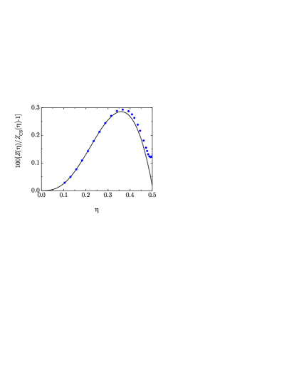
Figure 1: Plot of the relative deviation from the CS EOS, $100[Z(\eta)/Z_{\text{CS}}(\eta)-1]$. The solid line corresponds to the branch-point approximant (50), while the circles represent MD simulation data from Ref. Kolafa, Labík, and Malijevský, 2004. Adapted from Fig. 2 of Ref. Santos and  López de Haro, 2009.

At this stage it is worthwhile recalling that the EOS for hard hyperspheres in odd dimensions greater than $3$ derived from the PY integral equation possesses a branch-point singularity on the negative real axis that is responsible for the radius of convergence and the alternating character of the virial series.Freasier and Isbister (1981); Leutheusser (1984); González, González, and Silbert (1990); Bishop, Masters, and Clarke (1999); Rohrmann and Santos (2007); Rohrmann et al. (2008); Adda-Bedia, Katzav, and Vella (2008) It is very likely that these features are not artifacts of the PY approximation but would be shared by the exact EOS. However, in the case of the three-dimensional HS fluid, the radius of convergence of the PY EOS is artificially $\eta_{\text{conv}}=1$ and there is no definite indication about the nature of the singularity responsible for the true radius of convergence or its value.Clisby and McCoy (2006) With this in mind, a heuristic EOS for monocomponent HS systems was proposedSantos and  López de Haro (2009) that relied on the notion that the radius of convergence of the virial series might be dictated by a branch-point singularity. It reads

$$Z(\eta)=\frac{1+\sum_{k=0}^{3}u_{k}\eta^{k}-u_{0}\left(1+2v_{1}\eta+v_{2}\eta^{2}\right)^{3/2}}{(1-\eta)^{3}},$$ (50)

where $u_{0}$–$u_{3}$, $v_{1}$, and $v_{2}$ are parameters to be determined. The functional form (50) is general enough as to include the PY EOS from the virial and compressibility routes, and thus also the CS EOS, by setting $v_{2}=v_{1}^{2}$, $u_{1}=1+3u_{0}v_{1}$, $u_{2}=1+3u_{0}v_{1}^{2}$, and $u_{3}=b_{4}-19+u_{0}v_{1}^{3}$ with $b_{4}\equiv B_{4}/(\frac{\pi}{6}\sigma^{3})^{3}=16$, $19$, and $18$ for $Z_{\text{PY,v}}$, $Z_{\text{PY,c}}$, and $Z_{\text{CS}}$, respectively. On the other hand, if the parameters in Eq. (50) are determined by requiring agreement with the first seven virial coefficients, the resulting EOSSantos and  López de Haro (2009) successfully accounts for deviations of the CS EOS from molecular dynamics (MD) simulation values,Kolafa, Labík, and Malijevský (2004) as shown in Fig. 1.

Table 2: Expressions for $z_{2}(\eta)$, $\beta_{T}a_{2}(\eta)$, $X_{2}(\eta)$, and $X_{3}(\eta)$, as obtained from the PY solution for multicomponent HS fluids via different routes, as well as from the BMCSL approximation.

Route	$z_{2}(\eta)$	$\beta_{T}a_{2}(\eta)$	$X_{2}(\eta)$	$X_{3}(\eta)$
Virial	$\displaystyle{\frac{3\eta^{2}}{(1-\eta)^{2}}}$	$\displaystyle{\frac{3\eta}{1-\eta}+3\ln(1-\eta)}$	$\displaystyle{\frac{9\eta}{1-\eta}+9\ln(1-\eta)}$	$\displaystyle{-\frac{3\eta(2-3\eta)}{(1-\eta)^{2}}-6\ln(1-\eta)}$
Compressibility	$\displaystyle{\frac{3\eta^{2}}{(1-\eta)^{3}}}$	$\displaystyle{\frac{3\eta^{2}}{2(1-\eta)^{2}}}$	$\displaystyle{\frac{9\eta^{2}}{2(1-\eta)^{2}}}$	$\displaystyle{\frac{3\eta^{3}}{(1-\eta)^{3}}}$
$\mu$	$\displaystyle{-\frac{9(2-{3}\eta)}{2(1-\eta)^{2}}-\frac{9}{\eta}\ln(1-\eta)}$	$\displaystyle{\frac{9(2-\eta)}{2(1-\eta)}+\frac{9}{\eta}\ln(1-\eta)}$	$\displaystyle{\frac{9\eta^{2}}{2(1-\eta)^{2}}}$	$0$
BMCSL	$\displaystyle{\frac{\eta^{2}(3-\eta)}{(1-\eta)^{3}}}$	$\displaystyle{\frac{\eta}{(1-\eta)^{2}}+\ln(1-\eta)}$	$\displaystyle{\frac{3\eta}{(1-\eta)^{2}}+3\ln(1-\eta)}$	$\displaystyle{-\frac{\eta(2-5\eta+\eta^{2})}{(1-\eta)^{3}}-2\ln(1-\eta)}$

Now we turn to the multicomponent case. The contact values of the RDF in the PY approximation are given by

$$\bar{g}_{ij}=\frac{1}{1-\eta}+\frac{3}{2}\frac{\eta}{(1-\eta)^{2}}\frac{\sigma_{i}\sigma_{j}}{\sigma_{ij}}\frac{M_{2}}{M_{3}}.$$ (51)

The thermodynamic quantities are of course sensitive to the route followed to derive them. On the other hand, regardless of the route, they have the following common formSantos (2016); Heyes and Santos (2016, 2018)

$$Z=\frac{1}{1-\eta}+\frac{3\eta}{(1-\eta)^{2}}\frac{m_{2}}{m_{3}}+z_{2}(\eta)\frac{m_{2}^{3}}{m_{3}^{2}},$$ (52a)

$${\beta_{T}a^{\text{ex}}}=-\ln(1-\eta)+\frac{3\eta}{1-\eta}\frac{m_{2}}{m_{3}}+\beta_{T}a_{2}(\eta)\frac{m_{2}^{3}}{m_{3}^{2}},$$ (52b)

$$\beta_{T}\mu_{i}^{\text{ex}}= -\ln(1-\eta)+\frac{3\eta}{(1-\eta)^{2}}\frac{m_{2}}{m_{3}}\frac{\sigma_{1}}{M_{1}}$$

$$+\left[\frac{3\eta}{1-\eta}\frac{m_{2}}{m_{3}}+X_{2}(\eta)\frac{m_{2}^{3}}{m_{3}^{2}}\right]\frac{\sigma_{i}^{2}}{M_{2}}$$

$$+\left[\frac{\eta}{1-\eta}+\frac{3\eta^{2}}{(1-\eta)^{2}}\frac{m_{2}}{m_{3}}+X_{3}(\eta)\frac{m_{2}^{3}}{m_{3}^{2}}\right]\frac{\sigma_{i}^{3}}{M_{3}}.$$ (52c)

Therefore, only the coefficients of the combination of moments ${m_{2}^{3}}/{m_{3}^{2}}$ depend on the route. The explicit expressions of $z_{2}$, $a_{2}$, $X_{2}$ and $X_{3}$, according to the PY virial, compressibility, and $\mu$ routes are displayed in Table 2. Consistency with the single-component case (here denoted with the subscript s) gives

$$z_{2}(\eta)=Z_{\text{s}}(\eta)-\frac{1+2\eta}{(1-\eta)^{2}},$$ (53a)

$$\beta_{T}a_{2}(\eta)={\beta_{T}a^{\text{ex}}_{\text{s}}}+\ln(1-\eta)-\frac{3\eta}{1-\eta},$$ (53b)

$$X_{2}(\eta)+X_{3}(\eta)={\beta_{T}\mu^{\text{ex}}_{\text{s}}}+\ln(1-\eta)-\frac{\eta(7-4\eta)}{(1-\eta)^{2}}.$$ (53c)

Taking into account Eq. (48b), the following relationship holds

$$X_{2}(\eta)+X_{3}(\eta)=\beta_{T}a_{2}(\eta)+z_{2}(\eta).$$ (54)

This in turn implies that the multicomponent extension of Eq. (48) holds, namely,

$$\sum_{i=1}^{n_{c}}x_{i}\beta_{T}\mu_{i}= \frac{\partial(\eta\beta_{T}a)}{\partial\eta}$$ (55a)

$$= {\beta_{T}a}+Z.$$ (55b)

Figure 2: Plot of the compressibility factor $Z$ as a function of the mole fraction $x_{2}$ for a HS binary mixture with a packing fraction $\eta=0.49$ and size ratios (a) $\sigma_{1}/\sigma_{2}=0.6$ and (b) $\sigma_{1}/\sigma_{2}=0.3$. Symbols are MC computer simulation values,Barošová et al. (1996) while the lines stand for (from top to bottom) $Z_{\text{PY,c}}$, $Z_{\text{PY,c}\mu}$ [see Eq. (56)], $Z_{\text{BMCSL}}$, $Z_{\text{PY},\mu}$, and $Z_{\text{PY,v}}$, respectively. Note that $Z_{\text{PY,c}\mu}$ and $Z_{\text{BMCSL}}$ are hardly distinguishable. Panels (a) and (b) are adapted from Figs. 7.9 and 7.10, respectively, of Ref. Santos, 2016.

If an interpolation between the virial and compressibility routes analogous to that of Eq. (II.2.3) is carried out, one arrives at the widely used and rather accurate Boublík–Mansoori–Carnahan–Starling–Leland (BMCSL) EOSBoublík (1970); Mansoori et al. (1971) for HS mixtures. The associated coefficients $z_{2}$, $\beta_{T}a_{2}$, $X_{2}$ and $X_{3}$ are also included in Table 2. They are consistent with Eq. (53) if the single-component quantities are those of the CS EOS. Since the $\mu$ route turns out to be more accurate than the virial route, it seems natural to propose an alternative interpolation formula asSantos and Rohrmann (2013); Santos (2016)

$$Z_{\text{PY,c}\mu}=\frac{11}{18}Z_{\text{PY,c}}+\frac{7}{18}Z_{\text{PY,v}}.$$ (56)

As an assessment of the performance of the compressibility factors related to the PY solution, Fig. 2 compares them against Monte Carlo (MC) computer simulationsBarošová et al. (1996) for binary mixtures at $\eta=0.49$ and two values of the size ratio $\sigma_{1}/\sigma_{2}$. It is observed that $Z_{\text{PY,v}}$ underestimates the simulation values, while $Z_{\text{PY,c}}$ overestimates them. The $\mu$ route compressibility factor, $Z_{\text{PY,c}\mu}$, lies below the simulation data, but, as said before, it exhibits a better behavior than the virial route. The weighted average between $Z_{\text{PY,c}}$ and $Z_{\text{PY,v}}$ made in the construction of the BMCSL EOS does a very good job. A slightly better agreement is obtained from the weighted average between $Z_{\text{PY,c}}$ and $Z_{\text{PY,}\mu}$ [see Eq. (56)].

A comment is now in order. In the virial route, the starting point is the compressibility factor $Z$, as seen from Eq. (37b). Next, the Helmholtz free energy and chemical potential can be derived by standard thermodynamic relations, as summarized by the sequence

$$\begin{array}[]{l}Z\to\displaystyle{\int_{0}^{1}dt\frac{Z(\eta t)-1}{t}}=\displaystyle{{\beta_{T}a^{\text{ex}}}}\\ \hskip 113.81102pt\downarrow\\ \hskip 71.13188pt\displaystyle{\mu_{i}^{\text{ex}}=\frac{\partial(\rho a^{\text{ex}})}{\partial\rho_{i}}}.\end{array}$$ (57)

In the first step, use has been made of Eq. (17). In the case of the compressibility route [see Eq. (28)], use of the thermodynamic relation

$$\chi^{-1}=\frac{\partial\left(\eta Z\right)}{\partial\eta}$$ (58)

allows one to obtain the compressibility factor from the isothermal susceptibility as $Z=\int_{0}^{1}dt\,\chi^{-1}(\eta t)$. Thereafter, the sequence (57) applies again. On the other hand, in the $\mu$ route [Eq. (29b)], one first obtains the chemical potential of any species $i$. Next, the free energy and the compressibility factor are found by means of the sequence

$$\begin{array}[]{l}\{\mu_{i}^{\text{ex}}\}\to\displaystyle{\int_{0}^{1}dt\,\sum_{i=1}^{n_{c}}x_{i}\mu_{i}^{\text{ex}}(\eta t)}=\displaystyle{{a^{\text{ex}}}}\\ \hskip 142.26378pt\downarrow\\ \hskip 56.9055pt\displaystyle{Z-1=\sum_{i=1}^{n_{c}}x_{i}\beta_{T}\mu_{i}^{\text{ex}}-{\beta_{T}a^{\text{ex}}}},\end{array}$$ (59)

where in the first and second steps use has been made of Eqs. (55a) and (55b), respectively. Once the free energy is obtained from the $\mu$ route by the thermodynamic relation (55a), one might go back and derive the chemical potential of species $i$ via the thermodynamic relation in the second step of Eq. (57). As yet another instance of thermodynamic inconsistency, the resulting expression for $\beta_{T}\mu_{i}^{\text{ex}}$ differs from the original one in that $X_{2}\to X_{2}+\Delta X$ and $X_{3}\to X_{3}-\Delta X$ with $\Delta X=9(6-9\eta+2\eta^{2})/2(1-\eta)^{2}+54\ln(1-\eta)/2\eta$.Santos and Rohrmann (2013)

II.2.4 Phase behavior

The investigation of the phase diagram of the HS fluid has mainly relied on numerical simulations. Since the system is athermal, the only parameter controlling the phase behavior of the single-component system is the density or, equivalently, the packing fraction. Presently, the accepted view is that the phase diagram of the HS system is constituted by four main branches. The first one, which goes from $\eta=0$ to the freezing packing fraction $\eta_{\text{f}}\simeq 0.492$,Alder and Wainwright (1957); Fernández et al. (2012) represents the stable fluid branch. There is then a tie line that joins the freezing point and the melting point at the packing fraction $\eta_{\text{m}}\simeq 0.543$Hoover and Ree (1968); Fernández et al. (2012) in which there is fluid–solid coexistence. Above the melting point, the stable HS system is in a crystalline phase that ends at a close-packed face-centered cubic phase with a packing fraction $\eta_{\text{cp}}=\frac{\pi}{3\sqrt{2}}$.Speedy (1998) There is also a metastable fluid branch that extends past the freezing point and is conjectured to end at the densest possible random packing,Torquato (2018) namely, with a “jamming” packing fraction $\eta_{\text{J}}\simeq 0.64$. Finally, on the basis of experimental results on colloidal HSvan Megen and Underwood (1993); van Blaaderen and Wiltzius (1995) (which easily form glasses) and some theoretical developments,Speedy (1994); Yeo (1995) it has been concluded that a glass transition also occurs in the system at a packing fraction $\eta_{\text{g}}\simeq 0.58$ intermediate between $\eta_{\text{f}}$ and $\eta_{\text{J}}$—despite some controversy.

Evidence coming from the use of approximate EOS indicates that the freezing transition observed in computer simulations does not show up as a singularity in those approximations.Aguilera-Navarro et al. (1984) Moreover, while it is quite plausible that $Z(\eta)$ presents a singularity at the freezing density $\eta_{\text{f}}$,Gaunt and Joyce (1980); Joyce (1988); Baxter, Enting, and Tsang (1980) the virial coefficients (or even their asymptotic behavior) do not seem to yield either any information concerning the freezing transition at $\eta_{\text{f}}$.Gaunt and Joyce (1980) This might be related to the fact that $Z(\eta)$ remains finite when $\eta$ approaches $\eta_{\text{f}}$ from below.

Next, we turn to the high-density behavior. It should be remarked that the compressibility factor of the HS fluid, both for the stable and metastable fluid phases, is a monotonically increasing function of the packing fraction.McCoy (2010) On the other hand, the fluid EOS, continued and extrapolated beyond the fluid–solid transition, is expected to have a divergence to infinity at a certain packing fraction $\eta=\eta_{\infty}$, i.e,

$$\lim_{\eta\to\eta_{\infty}}Z_{\text{fluid}}(\eta)=\infty,\quad\eta_{\text{conv}}\leq\eta_{\infty}\leq\eta_{\text{cp}},$$ (60)

where we recall that $\eta_{\text{conv}}$ is the packing fraction corresponding to the radius of convergence of the virial series. By studying the singularities of Padé approximants constructed from the virial series for HS, SanchezSanchez (1994) came to the conclusion that such a singularity was related to the crystalline close-packing in these systems, i.e.,

$$\eta_{\infty}=\eta_{\text{cp}}.$$ (61)

Other authorsWoodcock (1976); Andrews (1975, 1976); Baram and Luban (1979); Devore and Schneider (1982); Aguilera-Navarro et al. (1983); Hoste and Van Dael (1984); Goldman and White (1988); Wang, Mead, and de Llano (1991); Santos, López de Haro, and Yuste (1995); López de Haro, Santos, and Yuste (1998); Wang, Khoshkbarchi, and Vera (1996); Khoshkbarchi and Vera (1997); Nasrifar, Ayatollahi, and Moshfeghian (2000); Ghotbi and Vera (2001); Wang (2002); Polishuk and Vera (2005); Miandehy, Modarress, and Dehghani (2006) have also conjectured Eq. (61). It is interesting to note that this conjecture was already suggested by KortewegKorteweg (1892) and BoltzmannBoltzmann (1898) in the late 1800s. On the other hand, the conjecture (61) has not been free from criticismGaunt and Joyce (1980) and some authorsLe Fevre (1972); Aguilera-Navarro et al. (1982); Ma and Ahmadi (1986); Song, Stratt, and Mason (1988); Hamad (1997); Hamad and Yahaya (2000) have conjectured that $\eta_{\infty}=\eta_{\text{J}}$.Berryman (1983) For a thorough account of proposed EOS, including those enforcing $\eta_{\infty}=\eta_{\text{cp}}$ or $\eta_{\infty}=\eta_{\text{J}}$, see Ref.  Mulero et al., 2008. It has also been shownMaestre et al. (2011) that the use of the direct Padé approximants of the compressibility factor $Z$ is not reliable for the purpose of determining $\eta_{\infty}$. Instead, one should consider an approach in which the independent variable is the pressure rather than the density. The analysis shows that the knowledge of the first twelve virial coefficients is not enough to decide whether $\eta_{\infty}=\eta_{\text{cp}}$ or $\eta_{\infty}=\eta_{\text{J}}$.

Once we have dealt with the one-component system, we now close this section by discussing the problem of fluid–fluid demixing in HS mixtures in which the knowledge about the virial coefficients is also valuable. An analysis of the solution of the PY integral equation for binary additive HS mixturesLebowitz and Rowlinson (1964) leads to the conclusion that no phase separation into two fluid phases exists in these systems. The same conclusion is reached if one considers the BMCSL EOS.Boublík (1970); Mansoori et al. (1971) For a long time the belief was that this was a true physical feature. Nevertheless, this belief started to be seriously questioned after Biben and HansenBiben and Hansen (1991) obtained fluid–fluid segregation in such mixtures out of the solution of the OZ equation with the Rogers–Young closure,Rogers and Young (1984) provided the size disparity was large enough. More recently, an accurate EOS derived by invoking some consistency conditionsSantos (2012b) does predict phase separation. The importance of this issue resides in the fact that if fluid–fluid phase separation occurs in additive HS binary mixtures, it must certainly be entropy driven. In contrast, in other mixtures such as molecular mixtures, temperature plays a non-neutral role and demixing is a free-energy driven phase transition.

The demixing problem has received a lot of attention in the literature in different contexts and using different approaches. For instance, Coussaert and BausCoussaert and Baus (1997, 1998) have proposed an EOS with improved virial behavior for a binary HS mixture that predicts a fluid–fluid transition at very high pressures (metastable with respect to a fluid–solid one). On the other hand, Regnaut et al.Regnaut, Dyan, and Amokrane (2001) have examined the connection between empirical expressions for the contact values of the pair distribution functions and the existence of fluid–fluid separation in HS mixtures. Finally, in the case of highly asymmetric binary additive HS mixtures, the depletion effect has been invoked as the physical mechanism behind demixing (see Refs. Dijkstra, van Roij, and Evans, 1998, 1999a, 1999b; Ayadim and Amokrane, 2006; Ashton et al., 2011 and the bibliography therein) and an effective one-component fluid description has been employed.

In two instances, namely, the limiting cases of a pure HS system and that of a binary mixture in which one of the species consists of point particles, it is known that there is no fluid–fluid separation.Vega (1998) For size ratios $\sigma_{1}/\sigma_{2}$ other than $1$ or $0$, one can find the spinodal instability curve (whose minimum determines the critical consolute point) by considering the truncated virial series. The resultsVlasov and Masters (2003); López de Haro and Tejero (2004); López de Haro, Malijevský, and Labík (2010) show that the values of the critical pressure and packing fraction monotonically increase with the truncation order. Extrapolation of these values to infinite truncation order suggests that the critical pressure diverges to infinity and the critical packing fraction tends towards its close-packing value, thus supporting a non-demixing scenario. This shows the extreme sensitivity of the demixing phenomenon to slight changes in the approximate EOS that is chosen to describe the mixture.

The argument that the truncated virial series are prone to exhibit demixing, albeit with larger and larger critical pressures, can be reinforced by analyzing a binary mixture in which one of the species consists of point particles. In that limit, the virial coefficients of the mixture are directly related to the ones of the pure fluid, which are known up to the twelfth.van Rensburg (1993); Labík, Kolafa, and Malijevský (2005); Clisby and McCoy (2005, 2006); Wheatley (2013) As mentioned previously, this system is known to lack a demixing transitionVega (1998) but the truncated virial series exhibits artificial critical points with the same qualitative features as observed for the mixtures with nonzero size ratios.López de Haro, Malijevský, and Labík (2010)

Therefore, one can conclude that a stable demixing fluid–fluid transition does not occur in (three-dimensional) additive binary HS mixtures but it is preempted by a fluid–solid transition.Dijkstra, van Roij, and Evans (1999b)

III The Rational Function Approximation (RFA) Method for the Structure of HS Fluids

We have already pointed out that, apart from requiring, in general, hard numerical labor, a disappointing aspect of the usual approach to obtain $g(r)$, namely, the integral equation approach, in which the OZ equation is complemented by a closure relation between $c(r)$ and $h(r)$,Barker and Henderson (1976) is that the substitution of the (necessarily) approximate values of $g(r)$ obtained from them in the (exact) statistical–mechanical formulae may lead to the thermodynamic consistency problem. In this section (which follows very closely material in Ref. López de Haro, Yuste, and Santos, 2008), we describe the RFA method for HS fluids, which is an alternative to the integral equation approach and in particular leads by construction to thermodynamic consistency between the virial and compressibility routes.

III.1 The single component HS fluid

III.1.1 General framework

We begin with the case of a HS single-component fluid. The following presentation is equivalent to the one given in Refs. Yuste and Santos, 1991; Yuste, López de Haro, and Santos, 1996, where all details can be found, but more suitable than the former for direct generalization to the case of mixtures.

The starting point will be the Laplace transform

$$G(s)=\int_{0}^{\infty}dr\,e^{-sr}rg(r).$$ (62)

The Fourier transform of the total correlation function is related to $G(s)$ by

$$\widetilde{h}(q)= \frac{4\pi}{q}\int_{0}^{\infty}dr\,r\sin(qr)h(r)$$

$$= -2\pi\left.\frac{G(s)-G(-s)}{s}\right|_{s=\imath q}.$$ (63)

Without loss of generality, we can define an auxiliary function $\Psi(s)$ through

$$G(s)=\frac{s}{2\pi}\left[\rho+e^{s\sigma}\Psi(s)\right]^{-1}.$$ (64)

The choice of $G(s)$ as the Laplace transform of $rg(r)$ and the definition of $\Psi(s)$ from Eq. (64) are suggested by the exact form of $g(r)$ [see Eq. (45a)] to first order in density.Yuste and Santos (1991)

Since $g(r)=0$ for $r<\sigma$, while $\bar{g}=\text{finite}$, one has

$$g(r)=\Theta(r-\sigma)\left[\bar{g}+(r-\sigma)\bar{g}^{\prime}+\cdots\right].$$ (65)

This property imposes a constraint on the large-$s$ behavior of $G(s)$, namely,

$$e^{\sigma s}sG(s)=\sigma\bar{g}+\left(\bar{g}+\sigma\bar{g}^{\prime}\right)s^{-1}+{\cal O}(s^{-2}).$$ (66)

Therefore, $\lim_{s\to\infty}e^{s\sigma}sG(s)=\sigma\bar{g}=\text{finite}$ or, equivalently,

$$\lim_{s\to\infty}s^{-2}\Psi(s)=\frac{1}{2\pi\sigma\bar{g}}=\text{finite}.$$ (67)

On the other hand, according to Eq. (12),

$$\chi= 1-24\eta\sigma^{-3}\lim_{s\to 0}\frac{\partial}{\partial s}\int_{0}^{\infty}dr\,e^{-sr}r\left[g(r)-1\right]$$

$$= 1-24\eta\sigma^{-3}\lim_{s\to 0}\frac{\partial}{\partial s}\left[G(s)-s^{-2}\right].$$ (68)

Since the isothermal susceptibility $\chi$ is also finite, one has $\int_{0}^{\infty}dr\,r^{2}\left[g(r)-1\right]=\text{finite}$, so that the weaker condition $\int_{0}^{\infty}dr\,r\left[g(r)-1\right]=\lim_{s\to 0}[G(s)-s^{-2}]=\text{finite}$ must hold. This in turn implies

$$e^{\sigma s}\Psi(s)=-\rho+\frac{s^{3}}{2\pi}+{\cal O}(s^{5}).$$ (69)

Note that Eq. (64) can be formally rewritten as

$$G(s)=\frac{s}{2\pi}\sum_{n=1}^{\infty}(-\rho)^{n-1}\left[\Psi(s)\right]^{-n}e^{-ns\sigma}.$$ (70)

Thus, the RDF is then given by

$$g\left({r}\right)=\frac{1}{2\pi r}\sum_{n=1}^{\infty}(-\rho)^{n-1}\psi_{n}\left(r-n\sigma\right)\Theta\left(r-n\sigma\right),$$ (71)

where

$$\psi_{n}\left(r\right)=\mathcal{L}^{-1}\left\{s\left[\Psi\left(s\right)\right]^{-n}\right\},$$ (72)

$\mathcal{L}^{-1}$ denoting the inverse Laplace transform.

Let us now derive an interesting property. For large $s$, Eq. (67) implies that $s\left[\Psi(s)\right]^{-n}\approx\left(2\pi\sigma\bar{g}\right)^{n}s^{-2n+1}$. This in turn implies the small-$r$ behavior $\psi_{n}(r)\approx\left(2\pi\sigma\bar{g}\right)^{n}r^{2n-2}/(2n-2)!$. Next, from Eq. (71) we find that the RDF exhibits $(2n-2)$th-order jump discontinuities at $r=n\sigma$, with $n=1,2,\ldots$, namely,

$$\lim_{r\to n\sigma^{+}}\frac{\partial^{2n-2}g(r)}{\partial r^{2n-2}}- \lim_{r\to n\sigma^{-}}\frac{\partial^{2n-2}g(r)}{\partial r^{2n-2}}$$

$$=\frac{(-12\eta)^{n-1}\bar{g}^{n}}{\sigma^{2n-2}n}.$$ (73)

As exemplified by Eq. (45), the exact RDF is also singular at some noninteger distances (in units of $\sigma$), such as $r=\sqrt{3}\sigma$.

Thus far, Eqs. (62)–(III.1.1) are formally exact, the auxiliary function $\Psi(s)$ remaining unknown.

Let us now consider a class of approximations where $\Psi(s)$ is an algebraic function, so that all the real-space functions $\psi_{n}\left(r\right)$ are regular for $r>0$. Under that condition, it is proved in Appendix A that the the only singularities of $h(r)$ are located at $r=n\sigma$ (with $n=1,2,\ldots$) and the DCF $c(r)$ is regular for any distance $r>\sigma$.

Among the class of algebraic-function approximations for $\Psi(s)$, let us focus on the subclass made of rational-function approximations (RFA), namely,

$$\Psi(s)=\frac{\sum_{\ell=0}^{\nu+2}S^{(\ell)}s^{\ell}}{\sum_{\ell=0}^{\nu}L^{(\ell)}s^{\ell}}.$$ (74)

The difference between the degree of the numerator ($\nu+2$) and that of the denominator ($\nu$) is fixed by the physical requirement (67). Since one of the coefficients in Eq. (74) can be freely chosen, the number of independent coefficients is $2\nu+3$. Next, the basic condition (69) fixes the first five coefficients in the expansion of $\Psi(s)$ in powers of $s$, so that $2\nu+3\geq 5$ or, equivalently, $\nu\geq 1$.

Enforcement of Eq. (69) up to order $s^{2}$ allows one to express $S^{(0)}$, $S^{(1)}$, and $S^{(2)}$ in terms of $L^{(0)}$, $L^{(1)}$, and $L^{(2)}$,

$$S^{(0)}=-\rho L^{(0)},$$ (75a)

$$S^{(1)}=-\rho\left[L^{(1)}-\sigma L^{(0)}\right],$$ (75b)

$$S^{(2)}=-\rho\left[L^{(2)}-\sigma L^{(1)}+\frac{1}{2}\sigma^{2}L^{(0)}\right].$$ (75c)

As a consequence, insertion of (74) into Eq. (64) yields

$$G(s)= \frac{e^{-\sigma s}}{2\pi s^{2}}\sum_{\ell=0}^{\nu}L^{(\ell)}s^{\ell}$$

$$\times\left[\sum_{\ell=3}^{\nu+2}S^{(\ell)}s^{\ell-3}-\rho\sum_{\ell=0}^{\nu}\varphi_{2-\ell}(\sigma s)\sigma^{3-\ell}L^{(\ell)}\right]^{-1},$$ (76)

where

$$\varphi_{\ell}(x)\equiv\begin{cases}\displaystyle{\frac{\sum_{k=0}^{\ell}\frac{(-x)^{k}}{k!}-e^{-x}}{x^{\ell+1}}},&\ell\geq 0,\\ \displaystyle{-\frac{e^{-x}}{x^{\ell+1}}},&\ell\leq-1\end{cases}.$$ (77)

Note that $\lim_{x\to 0}\varphi_{\ell}(x)=(-1)^{\ell}/(\ell+1)!$ and $0$ for $\ell\geq-1$ and $\ell\leq-2$, respectively. The requirement (69) to orders $s^{3}$ and $s^{4}$ provide $L^{(0)}$ and $L^{(1)}$ in terms of $L^{(2)}$, $L^{(3)}$, $L^{(4)}$, $S^{(3)}$, and $S^{(4)}$. Therefore, $L^{(j)}$ and $S^{(j+1)}$ for $j\geq 2$ remain free.

By application of the residue theorem, the functions defined in Eq. (72) are explicitly given by

$$\psi_{n}\left(r\right)=\sum_{m=1}^{n}\frac{\sum_{i=1}^{\nu+2}\bar{\psi}_{mn}^{(i)}e^{s_{i}r}}{\left(n-m\right)!(m-1)!}r^{n-m},$$ (78)

where

$$\bar{\psi}_{mn}^{(i)}\equiv\lim_{s\rightarrow s_{i}}\left(\frac{\partial}{\partial s}\right)^{m-1}s\left[\frac{\Psi\left(s\right)}{s-s_{i}}\right]^{-n},$$ (79)

$s_{i}$ ($i=1,\ldots,\nu+2$) being the roots of $\sum_{\ell=0}^{\nu+2}S^{(\ell)}s^{\ell}=0$.

III.1.2 First-order approximation (PY solution)

As seen above, the RFA (74) with the least number of coefficients to be determined corresponds to $\nu=1$, namely,

$$\Psi(s)=\frac{S^{(0)}+S^{(1)}s+S^{(2)}s^{2}+s^{3}}{L^{(0)}+L^{(1)}s},$$ (80)

where we have chosen $S^{(3)}=1$. With such a choice and in view of Eq. (69), one finds Eq. (75) with $L^{(2)}=0$ and

$$L^{(0)}=2\pi\frac{1+2\eta}{(1-\eta)^{2}},$$ (81a)

$$L^{(1)}=2\pi\sigma\frac{1+\eta/2}{(1-\eta)^{2}}.$$ (81b)

Finally, Eq. (III.1.1) becomes

$$G(s)=\frac{e^{-\sigma s}}{2\pi s^{2}}\frac{L^{(0)}+L^{(1)}s}{1-\rho\sum_{\ell=0}^{1}\varphi_{2-\ell}(\sigma s)\sigma^{3-\ell}L^{(\ell)}}.$$ (82)

It is remarkable that Eq. (82), which has been derived here as the simplest rational form for $\Psi(s)$ [see Eq. (74)] complying with the requirements (67) and (69), coincides with the solution to the PY closure of the OZ equationWertheim (1963) summarized in Sec. II.2.3. It is clear that this first-order approximation is not thermodynamically consistent.

III.1.3 Second-order approximation

In the spirit of the RFA (74), the second simplest implementation corresponds to $\nu=2$, thus involving two new terms, namely,

$$\Psi(s)=\frac{S^{(0)}+S^{(1)}s+S^{(2)}s^{2}+s^{3}+\alpha s^{4}}{L^{(0)}+L^{(1)}s+L^{(2)}s^{2}},$$ (83)

where again we have chosen $S^{(3)}=1$ and have called $S^{(4)}=\alpha$. Applying Eq. (69), one finds Eq. (75) and

$$L^{(0)}=2\pi\frac{1+2\eta}{(1-\eta)^{2}}+\frac{12\eta}{1-\eta}\left[\frac{\pi}{1-\eta}\frac{\alpha}{\sigma}-\frac{L^{(2)}}{\sigma^{2}}\right],$$ (84a)

$$L^{(1)}=2\pi\sigma\frac{1+\frac{1}{2}\eta}{(1-\eta)^{2}}+\frac{2}{1-\eta}\left[\pi\frac{1+2\eta}{1-\eta}\alpha-3\eta\frac{L^{(2)}}{\sigma}\right].$$ (84b)

Furthermore,

$$G(s)=\frac{e^{-\sigma s}}{2\pi s^{2}}\frac{L^{(0)}+L^{(1)}s+{L^{(2)}}s^{2}}{1+\alpha s-\rho\sum_{\ell=0}^{2}\varphi_{2-\ell}(\sigma s)\sigma^{3-\ell}L^{(\ell)}}.$$ (85)

Thus far, irrespective of the values of the coefficients $L^{(2)}$ and $\alpha$, the conditions $\lim_{s\to\infty}e^{\sigma s}sG(s)=\text{finite}$ [see Eq. (66)] and $\lim_{s\to 0}[G(s)-s^{-2}]=\text{finite}$ are satisfied. Of course, if $L^{(2)}=\alpha=0$, one recovers the PY approximation. More generally, we may determine these two coefficients by prescribing the compressibility factor $Z$ [or, equivalently, the contact value $\bar{g}$, see Eq. (42)] and the isothermal susceptibility $\chi$. This gives

$${L^{(2)}}={2\pi\alpha\sigma}\bar{g},$$ (86a)

$$\chi=\left[\frac{2\pi}{L^{(0)}}\right]^{2}\left[1-\frac{12\eta}{1-\eta}\frac{\alpha}{\sigma}\left(1+\frac{2\alpha}{\sigma}\right)+\frac{12\eta}{\pi}\frac{\alpha L^{(2)}}{\sigma^{3}}\right].$$ (86b)

In order to ensure thermodynamic consistency, it is convenient to fix the isothermal susceptibility $\chi$ from $Z$ by means of the thermodynamic relationship (58). Henceforth, we will restrict the use of the term RFA to this second-order approximation ($\nu=2$).

Upon substitution of Eqs. (84a) and (86a) into Eq. (86b) a quadratic algebraic equation for $\alpha$ is obtained. The physical root is

$$\alpha=\frac{(1+2\eta)R}{(1-\eta)(3Z-1)+3[(1-\eta)Z-1-\eta]R},$$ (87)

where

$$R\equiv\sqrt{1+\frac{Z-\frac{1}{3}}{Z-Z_{\text{PY,v}}}\left(\frac{\chi}{\chi_{\text{PY,c}}}-1\right)}-1.$$ (88)

Here, $Z_{\text{PY,v}}$ and $\chi_{\text{PY,c}}$ correspond to the PY expressions in the virial and compressibility routes, respectively (see Table 1). The other root of the quadratic equation must be discarded because it corresponds to a negative value of $\alpha$, which, according to Eq. (86a), yields a negative value of $L^{(2)}$. This would imply the existence of a positive real value of $s$ at which $G(s)=0$,Yuste and Santos (1991); Yuste, López de Haro, and Santos (1996) which is not compatible with a positive definite RDF.

A reasonable compressibility factor must be $Z>Z_{\text{PY,v}}$. Moreover, if the chosen EOS yields a diverging pressure at $\eta_{\infty}<1$, there must necessarily exist a certain packing fraction $\eta_{\text{g}}$ above which $\chi<\chi_{\text{PY,c}}$. As one approaches the value $\eta_{\text{g}}$ from below, so that $\chi/\chi_{\text{PY,c}}\to 1^{+}$, Eqs. (87) and (88) show that $R,\alpha\to 0$, both quantities becoming complex beyond $\eta=\eta_{\text{g}}$. This may be interpreted as an indication that, at the packing fraction $\eta_{\text{g}}$, the system ceases to be a fluid and a glass transition occurs.Yuste, López de Haro, and Santos (1996); Robles et al. (1998); Robles and de Haro (2003)

Expanding (85) in powers of $s$ and using Eq. (66) one can obtain the derivatives of the RDF at $r=\sigma^{+}$.Robles and López de Haro (1997) In particular, the first derivative is

$$\bar{g}^{\prime}=\frac{1}{2\pi\alpha\sigma}\left[L^{(1)}-L^{(2)}\left(\frac{1}{\alpha}+\frac{1}{\sigma}\right)\right],$$ (89)

which may have some use in connection with perturbation theory.Lee and Levesque (1973)

It is worthwhile pointing out that the structure implied by Eq. (85) coincides in this single-component case with the solution of the Generalized Mean Spherical Approximation (GMSA),Waisman (1973) where the OZ relation is solved under the ansatz that the DCF has a Yukawa form outside the core.

For given $Z$ and $\chi$, once $G(s)$ has been fully determined, the RDF in real space is given by Eqs. (71) and (78) with $\nu=2$. Explicit expressions of $g(r)$ up to the second coordination shell $\sigma\leq r\leq 3\sigma$ can be found in Ref. Díez, Largo, and Solana, 2006. Furthermore, the static structure factor $S(q)$ [cf. Eq. (8)] and the Fourier transform $\widetilde{h}(q)$ may be related to $G(s)$ from Eq. (III.1.1) (see also Appendix A). Therefore, the basic structural quantities of the single-component HS fluid, namely, the RDF and the static structure factor, may be analytically determined within the RFA method once the compressibility factor $Z$ (or, equivalently, the contact value $\bar{g}$) is specified.

In Fig. 3, we compare MD simulation dataKolafa, Labík, and Malijevský (2004) of $g(r)$ for a density $\rho\sigma^{3}=0.9$ with the RFA prediction and the parameterized approach by Trokhymchuk et al.,Trokhymchuk et al. (2005) where $Z=Z_{\text{CS}}$ [cf. Eq. (II.2.3)] and the associated isothermal susceptibility $\chi=\chi_{\text{CS}}$ (see Table 1) are taken in both cases. Both theories are rather accurate, but the RFA captures better the maxima and minima of $g(r)$.López de Haro, Santos, and Yuste (2006)

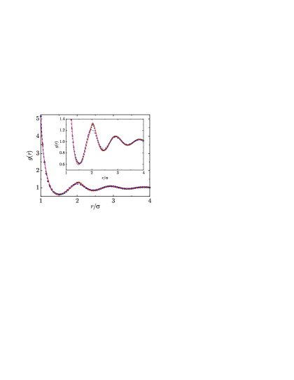
Figure 3: RDF of a single-component HS fluid for $\rho\sigma^{3}=0.9$ ($\eta=0.471$). The symbols represent MD simulation data,Kolafa, Labík, and Malijevský (2004) the dashed lines represent the results of the approach of Ref. Trokhymchuk et al., 2005, and the solid lines refer to those of the RFA method. The inset shows the oscillations of $g(r)$ in more detail. Adapted from Fig. 6.8 of Ref. López de Haro, Yuste, and Santos, 2008.

It is also possible to obtain the DCF $c(r)$ within the RFA method. Using Eqs. (19) and (III.1.1) [see also Eq. (A)], and applying the residue theorem, one gets, after some algebra,

$$c(r)= \Bigg{(}K_{+}\frac{e^{\kappa r^{*}}}{r^{*}}+K_{-}\frac{e^{-\kappa r^{*}}}{r^{*}}+\frac{K_{-1}}{r^{*}}+K_{0}+K_{1}r^{*}$$

$$+K_{3}{r^{*}}^{3}\Bigg{)}\Theta(1-r^{*})+K\frac{e^{-\kappa r^{*}}}{r^{*}},$$ (90)

where

$$\kappa=\frac{\sigma}{\alpha}\sqrt{\frac{12\eta\alpha L^{(2)}}{\pi\sigma^{3}}+1-\frac{12\alpha}{\sigma}\left(1+\frac{2\alpha}{\sigma}\right)\frac{\eta}{1-\eta}}$$ (91)

and the expressions for the amplitudes can be found in Appendix B. In contrast to the PY result [Eq.  (47c)], now the DCF does not vanish outside the hard core ($r>\sigma$) but has a Yukawa form in that region. Note that Eq. (166f) guarantees that $c(0)=\text{finite}$, while Eq. (166b) yields $\lim_{r\to\sigma^{+}}c(r)-\lim_{r\to\sigma^{-}}c(r)=L^{(2)}/2\pi\alpha=\bar{g}$. The latter proves the continuity of the indirect correlation function $\gamma(r)$ at $r=\sigma$. With the above results [Eqs. (71) and (III.1.3)], one may immediately write the function $\gamma(r)$. Finally, we note that, according to Eq. (21), the bridge function $b(r)$ is linked to $\gamma(r)$ and $y(r)$ through

$$b(r)=\ln y(r)-\gamma(r).$$ (92)

Thus, within the RFA method, the bridge function is also completely specified analytically for $r\geq\sigma$ once $Z$ is prescribed.

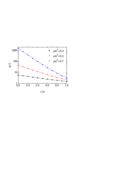
Figure 4: Cavity function of a single-component HS fluid in the overlap region for $\rho\sigma^{3}=0.3$, $0.5$, and $0.7$. The solid lines represent our proposal (95) with $Z=Z_{\text{CS}}$, while the symbols represent MC simulation results.Labík and Malijevský (1984) Adapted from Fig. 6.9 of Ref. López de Haro, Yuste, and Santos, 2008.

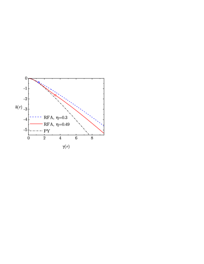
Figure 5: Parametric plot of the bridge function $b(r)$ vs the indirect correlation function $\gamma(r)$. The dashed line refers to the RFA for $\eta=0.3$, while the solid line refers to the RFA for $\eta=0.49$. In each case, the branch of the curve to the right of the circle corresponds to $r\leq\sigma$, while that to the left corresponds to $r\geq\sigma$. For comparison, the density-independent PY closure $b(r)=\ln[1+\gamma(r)]-\gamma(r)$ is also plotted (dash-dotted line). Adapted from Fig. 6.10 of Ref. López de Haro, Yuste, and Santos, 2008.

If one wants to have $b(r)$ also for $0\leq r\leq\sigma$, then an expression for the cavity function in that region is required. Here, we propose such an expression using a limited number of constraints. First, since the cavity function and its first derivative are continuous at $r=\sigma$, we have

$$y(\sigma)=\bar{g},\quad\frac{y^{\prime}(\sigma)}{y(\sigma)}=\frac{L^{(1)}}{L^{(2)}}-\frac{1}{\alpha}-\frac{1}{\sigma},$$ (93)

where Eqs. (86a) and (89) have been used. Next, we consider the following exact zero-separation theorems:Lee (1995); Lee, Ghonasgi, and Lomba (1996); Lee and Malijevský (2001)

$$\ln y(0)=Z-1+\int_{0}^{1}dt\frac{Z(\eta t)-1}{t},$$ (94a)

$$\frac{y^{\prime}(0)}{y(0)}=-6\eta\frac{y(\sigma)}{\sigma}.$$ (94b)

The four conditions (93)–(94) can be enforced by assuming a cubic polynomial form for $\ln y(r)$ inside the core, namely,

$$y(r)=\exp\left(Y_{0}+Y_{1}r^{*}+Y_{2}{r^{*}}^{2}+Y_{3}{r^{*}}^{3}\right),\quad 0\leq r\leq\sigma,$$ (95)

where

$$Y_{0}=Z-1+\int_{0}^{1}dt\frac{Z(\eta t)-1}{t},$$ (96a)

$$Y_{1}=-6\eta y(\sigma),$$ (96b)

$$Y_{2}=3\ln y(\sigma)-\frac{\sigma y^{\prime}(\sigma)}{y(\sigma)}-3Y_{0}-2Y_{1},$$ (96c)

$$Y_{3}=-2\ln y(\sigma)+\frac{\sigma y^{\prime}(\sigma)}{y(\sigma)}+2Y_{0}+Y_{1}.$$ (96d)

The proposal (95) is compared with available MC dataLabík and Malijevský (1984) in Fig. 4, where an excellent agreement can be observed.

Once the cavity function $y(r)$ provided by the RFA method is complemented by Eq. (95), the bridge function $b(r)$ can be obtained at any distance. Figure 5 presents a parametric plot of the bridge function vs the indirect correlation function as given by the RFA method for two different packing fractions, as well as the result associated with the PY closure. The fact that one gets a smooth curve means that, within the RFA, the oscillations in $\gamma(r)$ are highly correlated with those of $b(r)$. Further, the effective closure relation in the RFA turns out to be density dependent, in contrast with what occurs for the PY theory. Note that the absolute value $|b(r)|$ for a given value of $\gamma(r)$ is smaller in the RFA than the PY value. On the other hand, the RFA and PY curves become closer as the density increases. Since the PY theory is known to yield rather poor values of the cavity function inside the core,Malijevský and Santos (2006); Santos and Malijevský (2007) it seems likely that the present differences may represent yet another manifestation of the superiority of the RFA method.

III.2 The multicomponent HS fluid

The method outlined in Subsection III.1 will be now extended to an $n_{c}$-component mixture of additive HS. Similar to what we did in the single-component case, we introduce the Laplace transforms of $rg_{ij}(r)$,

$$G_{ij}(s)=\int_{0}^{\infty}dr\,e^{-sr}rg_{ij}(r),$$ (97)

so that the Fourier transform of $h_{ij}(r)$ can be obtained as

$$\widetilde{h}_{ij}(q)=-2\pi\left.\frac{G_{ij}(s)-G_{ij}(-s)}{s}\right|_{s=\imath q}.$$ (98)

The counterparts of Eqs. (65) and (66) are

$$g_{ij}(r)=\Theta(r-\sigma_{ij})\left[\bar{g}_{ij}+(r-\sigma_{ij})\bar{g}_{ij}^{\prime}+\cdots\right],$$ (99a)

$$e^{\sigma_{ij}s}sG_{ij}(s)=\sigma_{ij}\bar{g}_{ij}+\left(\bar{g}_{ij}+\sigma_{ij}\bar{g}_{ij}^{\prime}\right)s^{-1}+{\cal O}(s^{-2}).$$ (99b)

Moreover, according to Eq. (28), the condition of a finite compressibility implies that $\widetilde{h}_{ij}(0)=\text{finite}$. As a consequence, for small $s$,

$$s^{2}G_{ij}(s)=1+H_{ij}^{(0)}s^{2}+H_{ij}^{(1)}s^{3}+\cdots$$ (100)

with $H_{ij}^{(0)}=\text{finite}$ and $H_{ij}^{(1)}=-\widetilde{h}_{ij}(0)/4\pi=\text{finite}$, where

$$H_{ij}^{(n)}\equiv\frac{1}{n!}\int_{0}^{\infty}dr\,(-r)^{n}rh_{ij}(r).$$ (101)

We are now in the position to generalize the approximation (85) to the $n_{c}$-component case.Yuste, Santos, and López de Haro (1998); Malijevský et al. (2007); Yuste, Santos, and López de Haro (2008) While such a generalization may be approached in a variety of ways, two motivations are apparent. On the one hand, we want to recover the PY resultLebowitz (1964) as a particular case in much the same fashion as in the single-component system. On the other hand, we want to maintain the development as simple as possible. Taking all of this into account, we generalize Eq. (85) as

$$G_{ij}(s)=\frac{e^{-\sigma_{ij}s}}{2\pi s^{2}}\left({\sf L}(s)\cdot\left[(1+\alpha s)\mathsf{I}-{\sf A}(s)\right]^{-1}\right)_{ij},$$ (102)

where $\mathsf{L}(s)$ and $\mathsf{A}(s)$ are the matrices

$$L_{ij}(s)=L_{ij}^{(0)}+L_{ij}^{(1)}s+L_{ij}^{(2)}s^{2},$$ (103)

$$A_{ij}(s)=\rho_{i}\sum_{\ell=0}^{2}\varphi_{2-\ell}(\sigma_{i}s)\sigma_{i}^{3-\ell}L_{ij}^{(\ell)},$$ (104)

the functions $\varphi_{\ell}(x)$ being defined by Eq. (77). We note that, by construction, Eq. (102) complies with the requirement $\lim_{s\rightarrow\infty}e^{\sigma_{ij}s}sG_{ij}(s)=\text{finite}$. Further, in view of Eq. (100), the coefficients of $s^{0}$ and $s$ in the power series expansion of $s^{2}G_{ij}(s)$ must be $1$ and $0$, respectively. This yields $2n_{c}^{2}$ conditions that allow us to express ${\sf L}^{(0)}$ and ${\sf L}^{(1)}$ in terms of ${\sf L}^{(2)}$ and $\alpha$. The solution isYuste, Santos, and López de Haro (1998)

$$L_{ij}^{(0)}=\vartheta_{1}+\vartheta_{2}\sigma_{j}+2\vartheta_{2}\alpha-\vartheta_{1}\sum_{k=1}^{n_{c}}\rho_{k}\sigma_{k}L_{kj}^{(2)},$$ (105a)

$$L_{ij}^{(1)}= \vartheta_{1}\sigma_{ij}+\frac{1}{2}\vartheta_{2}\sigma_{i}\sigma_{j}+(\vartheta_{1}+\vartheta_{2}\sigma_{i})\alpha$$

$$-\frac{1}{2}\vartheta_{1}\sigma_{i}\sum_{k=1}^{n_{c}}\rho_{k}\sigma_{k}L_{kj}^{(2)},$$ (105b)

where $\vartheta_{1}\equiv 2\pi/(1-\eta)$ and $\vartheta_{2}\equiv 6\pi(m_{2}/m_{3})\eta/(1-\eta)^{2}$.

In parallel with the development of the single-component case, ${\sf L}^{(2)}$ and $\alpha$ can be chosen arbitrarily. Again, the choice $L_{ij}^{(2)}=\alpha=0$ gives the PY solution.Lebowitz (1964); Blum and Høye (1977) Since we want to go beyond this approximation, we will determine those coefficients by taking prescribed values for $\bar{g}_{ij}$, which in turn, via Eq. (37b), give the EOS of the mixture. This also leads to the required value of $\chi$ via Eq. (58), thus making the theory thermodynamically consistent. In particular, according to Eq. (99b),

$${L_{ij}^{(2)}}={2\pi\alpha\sigma_{ij}}\bar{g}_{ij}.$$ (106)

The condition related to $\chi$ is more involved. Making use of Eq. (100), one can get $\widehat{h}_{ij}(0)=-4\pi\rho\sqrt{x_{i}x_{j}}H_{ij}^{(1)}$ in terms of ${\sf L}^{(2)}$ and $\alpha$, and then insert it into Eq. (28). Finally, elimination of $L_{ij}^{(2)}$ in favor of $\alpha$ from Eq. (106) produces a polynomial equation of degree $2n_{c}$, whose physical root is determined by the requirement that $G_{ij}(s)$ is positive definite for positive real $s$. It turns out that the physical solution corresponds to the smallest of the real roots. Once $\alpha$ is known, upon substitution into Eqs. (102), (105), and (106), the scheme is complete. Also, using Eq. (99b), one can easily derive the result

$$\bar{g}_{ij}^{\prime}=\frac{1}{2\pi\alpha\sigma_{ij}}\left[L_{ij}^{(1)}-L_{ij}^{(2)}\left(\frac{1}{\alpha}+\frac{1}{\sigma_{ij}}\right)\right].$$ (107)

It is straightforward to check that the results of Sec. III.1.3 are recovered by setting $\sigma_{i}=\sigma$, regardless of the values of the mole fractions and the number of components.

Once $G_{ij}(s)$ has been determined, inverse Laplace transformation directly yields $rg_{ij}(r)$. Although, in principle, as in the single-component case, this can be done analytically, it is more practical to use one of the efficient methods discussed by Abate and WhittAbate and Whitt (1992) to numerically invert Laplace transforms.

From Eqs. (23) and (98) it is possible to obtain explicit expressions for $\widetilde{c}_{ij}(q)$. Subsequent numerical inverse Fourier transformation yields $c_{ij}(r)$. The indirect correlation functions $\gamma_{ij}(r)\equiv h_{ij}(r)-c_{ij}(r)$ readily follow from the previous results for the RDF and DCF. Finally, in this case the bridge functions $b_{ij}(r)$ for $r>\sigma_{ij}$ are linked to $g_{ij}(r)$ and $c_{ij}(r)$ throughYuste, Santos, and López de Haro (2000) $b_{ij}(r)=\ln g_{ij}(r)-\gamma_{ij}(r)$ and so we have a full set of structural properties of a multicomponent fluid mixture of HS once the contact values $g_{ij}(\sigma_{ij})$ are specified.

Figure 6: Plot of the contact value $\bar{g}_{ij}$ as a function of the parameter $z_{ij}$ [see Eq. (111)]. The circles are MC simulation dataMalijevský et al. (2002) for ternary additive HS mixtures with diameter ratios $\sigma_{2}/\sigma_{1}=2$ and $\sigma_{3}/\sigma_{1}=3$ at a packing fraction $\eta=0.49$ and mole fractions $(x_{1},x_{2},x_{3})=(0.70,0.20,0.10)$, $(0.60,0.20,0.30)$, $(0.86,0.11,0.03)$, $(0.85,0.05,0.10)$, and $(0.90,0.07,0.03)$. Lines are theoretical predictions: from bottom to top—PY [Eq. (51)], BGHLL [Eq. (109)], eCS2 [Eq. (110)], and SPT [Eq. (108)]. Adapted from Fig. 3 of Ref. Malijevský et al., 2002.

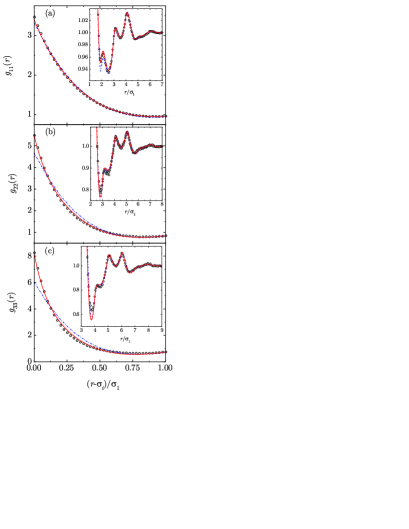
Figure 7: RDF (a) $g_{11}(r)$, (b) $g_{22}(r)$, and (c) $g_{33}(r)$ in the range $\sigma_{i}\leq r\leq\sigma_{i}+\sigma_{1}$ for a ternary HS mixture with diameter ratios $\sigma_{2}/\sigma_{1}=2$ and $\sigma_{3}/\sigma_{1}=3$ at a packing fraction $\eta=0.49$ and mole fractions $(x_{1},x_{2},x_{3})=(0.7,0.2,0.1)$. The circles are MC simulation results,Malijevský et al. (2002) the solid lines are RFA predictions, and the dash-dotted lines are PY predictions. The insets show in detail the oscillations in the region $\sigma_{i}\leq r\leq\sigma_{i}+6\sigma_{1}$. Adapted from Fig. 4 of Ref. Malijevský et al., 2002.

The PY prediction given by Eq. (51) underestimates the contact values and is not particularly accurate. On the other hand, the contact values obtained from the scaled particle theory (SPT) for mixtures,Reiss, Frisch, and Lebowitz (1959); Lebowitz, Helfand, and Praestgaard (1965); Mandell and Reiss (1975); Rosenfeld (1988); Heying and Corti (2004) namely,

$$\bar{g}_{ij}^{\text{SPT}}= \frac{1}{1-\eta}+\frac{3}{2}\frac{\eta}{(1-\eta)^{2}}\frac{\sigma_{i}\sigma_{j}}{\sigma_{ij}}\frac{M_{2}}{M_{3}}$$

$$+\frac{3}{4}\frac{\eta^{2}}{(1-\eta)^{3}}\left(\frac{\sigma_{i}\sigma_{j}}{\sigma_{ij}}\frac{M_{2}}{M_{3}}\right)^{2},$$ (108)

tend to overestimate the simulation values. Interestingly, insertion of Eq. (108) into Eq. (37b) yields an EOS that coincides with that of the PY solution in the compressibility route. BoublíkBoublík (1970) and, independently, Grundke and HendersonGrundke and Henderson (1972) and Lee and LevesqueLee and Levesque (1973) proposed an interpolation between the PY and the SPT contact values, that we will refer to as the BGHLL values,

$$\bar{g}_{ij}^{\text{BGHLL}}= \frac{1}{1-\eta}+\frac{3}{2}\frac{\eta}{(1-\eta)^{2}}\frac{\sigma_{i}\sigma_{j}}{\sigma_{ij}}\frac{M_{2}}{M_{3}}$$

$$+\frac{1}{2}\frac{\eta^{2}}{(1-\eta)^{3}}\left(\frac{\sigma_{i}\sigma_{j}}{\sigma_{ij}}\frac{M_{2}}{M_{3}}\right)^{2}.$$ (109)

This leads, via Eq.  (37b), to the widely used and rather accurate BMCSL EOS.Boublík (1970); Mansoori et al. (1971)

Refinements of the BGHLL values have been subsequently introduced, among others, by Henderson et al.,Henderson et al. (1996); Yau, Yu, and Henderson (1996); Henderson and Chan (1998a, b, 2000); Henderson et al. (1998); Matyushov, Henderson, and Chan (1999); Cao et al. (2000); Santos et al. (2009) Matyushov and Ladanyi,Matyushov and Ladanyi (1997) and Barrio and SolanaBarrio and Solana (2000) to eliminate some drawbacks of the BMCSL EOS in the so-called colloidal limit of binary HS mixtures. On a different path, but also having to do with the colloidal limit, Viduna and SmithViduna and Smith (2002a, b) have proposed a method to obtain contact values of the RDF of HS mixtures from a given EOS. However, most of these proposals are not easily generalized to the case of an arbitrary number of components. Yet another extension of the CS contact value to a mixture with an arbitrary number of components, different from Eq. (109), was proposed in Ref. Santos, Yuste, and López de Haro, 2002 (see also Sec. IV.2), specifically

$$\bar{g}_{ij}^{\text{eCS2}}= \frac{1}{1-\eta}+\frac{3}{2}\frac{\eta(1-\eta/3)}{(1-\eta)^{2}}\frac{\sigma_{i}\sigma_{j}}{\sigma_{ij}}\frac{M_{2}}{M_{3}}$$

$$+\frac{\eta^{2}(1-\eta/2)}{(1-\eta)^{3}}\left(\frac{\sigma_{i}\sigma_{j}}{\sigma_{ij}}\frac{M_{2}}{M_{3}}\right)^{2}.$$ (110)

Equations (51) and (108)–(110) have in common the fact that, at a given packing fraction $\eta$, the dependence of $\bar{g}_{ij}$ on the sets of diameters $\{\sigma_{k}\}$ and mole fractions $\{x_{k}\}$ takes place only through the scaled quantity

$$z_{ij}\equiv\frac{\sigma_{i}\sigma_{j}}{\sigma_{ij}}\frac{M_{2}}{M_{3}}.$$ (111)

Thus, at a fixed packing fraction, the contact values of different pairs and different mixtures should collapse onto a common curve when plotted vs $z_{ij}$. Figure 6 shows that this collapse property is reasonably well supported by MC data for the six pair contact values of each one of five ternary mixtures at $\eta=0.49$.Malijevský et al. (2002) The linear function (51) and the three quadratic functions (108)–(110) are also plotted. Comparison with the simulation data indicates that Eq. (110) performs generally better than Eq. (109), especially as $z_{ij}$ increases

Clearly, the use of any of these approximate contact values in the RFA approach will lead to (almost completely) analytical results for the structural properties of HS mixtures with the further asset that there will be full thermodynamic compatibility between the virial and compressibility routes. As an extra bonus, the (usually hard) numerical labor involved in the determination of the structural properties of these systems by solving integral equations is eliminated.

Figure 7 presents a comparison between the results of the RFA method with the PY theory and simulation dataMalijevský et al. (2002) for the like-like RDF of a ternary mixture. In the case of the RFA, we have used the eCS2 contact values and the corresponding isothermal susceptibility. The improvement of the RFA over the PY prediction, particularly in the region near contact, is noticeable. Although the RFA accounts nicely for the observed oscillations, it seems to somewhat overestimate the depth of the first minimum.

A recent comparison with MD simulationsPieprzyk et al. (2020) shows that the RFA is also rather accurate in predicting the DCF $c_{ij}(r)$ and the asymptotic large-$r$ behavior of the RDF $g_{ij}(r)$ for HS mixtures, including the so-called structural crossover transition.Evans et al. (1994); Statt et al. (2016)

IV Mappings of the EOS of the Single-Component HS Fluid onto the EOS of the HS Fluid Mixture

Obviously, it is, in principle, simpler to obtain the compressibility factor of the one-component fluid, $Z_{\text{s}}$, than that of a multicomponent mixture, $Z$. On the other hand, it is well known that a certain degree of polydispersity is enough to prevent crystallization in HS fluids. In this section we present the ideas we have followed to link the multicomponent compressibility factor, $Z$, and excess free energy per particle, $a^{\text{ex}}$, to their one-component counterparts $Z_{\text{s}}$ and $a_{\text{s}}^{\text{ex}}$. Among other things, this has allowed us to to examine (at least partially) the metastable fluid region of the monocomponent fluid.

IV.1 The e1 approximation

Of course, a straightforward way to obtain approximate expressions for the EOS of the mixture in terms of the EOS of the single-component fluid is simply by proposing or deriving approximate expressions for the contact values $\bar{g}_{ij}$ in terms of $\bar{g}_{\text{s}}$. We have already followed this route and the outcome is briefly described below. More details may be found in Refs. López de Haro, Yuste, and Santos, 2008; Santos, 2016 and references therein.

The basic assumption here is that, given a certain packing fraction $\eta$, the whole dependence of $\bar{g}_{ij}$ on the composition $\{\sigma_{k},x_{k}\}$ and number of components $n_{c}$ of the mixture occurs through the scaled quantity $z_{ij}$ defined in Eq. (111). More specifically,

$$\bar{g}_{ij}=\mathcal{G}(\eta,z_{ij}),$$ (112)

where the function $\mathcal{G}(\eta,z)$ is universal, i.e., it is a common function for all the pairs $(i,j)$, regardless of the composition and number of components of the mixture.

As mentioned in Sec. III, the PY, SPT, BGHLL, and eCS2 contact values belong to the class of approximations (112). Now, however, we want $\bar{g}_{\text{s}}$ to remain free, in contrast to what happens with Eqs. (51) and (108)–(110). This imposes the constraint

$$\mathcal{G}(\eta,1)=\bar{g}_{\text{s}}.$$ (113)

This means that the system is indistinguishable from a single-component one if all the sizes are identical ($\sigma_{i}=\sigma$ and $z_{ij}=1$).

Next, we consider the limit in which one of the species, say $i=0$, is made of point particles, i.e., $\sigma_{0}\rightarrow 0$. In that case, $\bar{g}_{00}$ takes the ideal-gas value, except that one has to take into account that the available volume for the point particles is not $V$ but $V(1-\eta)$. Thus,

$$\lim_{\sigma_{0}\rightarrow 0}\bar{g}_{00}=\frac{1}{1-\eta}.$$ (114)

Since $z_{00}\rightarrow 0$ in the limit $\sigma_{0}\rightarrow 0$, insertion of Eq. (114) into (112) yields

$$\mathcal{G}(\eta,0)=\frac{1}{1-\eta}.$$ (115)

As the simplest approximation of the class (112),Santos, Yuste, and López de Haro (1999) one may assume a linear dependence of $\mathcal{G}$ on $z$ that satisfies the basic requirements (113) and (115), namely,

$$\mathcal{G}(\eta,z)=\frac{1}{1-\eta}+\left(\bar{g}_{{\text{s}}}-\frac{1}{1-\eta}\right)z.$$ (116)

Inserting this into Eq. (112), one has

$$\bar{g}_{ij}^{\text{e1}}=\frac{1}{1-\eta}+\left(\bar{g}_{{\text{s}}}-\frac{1}{1-\eta}\right)\frac{\sigma_{i}\sigma_{j}}{\sigma_{ij}}\frac{M_{2}}{M_{3}}.$$ (117)

Here, the label “e1” is meant to indicate that (i) the contact values used are an extension of the single component contact value $\bar{g}_{{\text{s}}}$ and that (ii) $\mathcal{G}(\eta,z)$ is a linear polynomial in $z$. When Eq. (117) is inserted into Eq. (37b), one easily obtains

$$Z_{\text{e1}}(\eta)= 1+\left(1+\frac{m_{2}}{m_{3}}-2\frac{m_{2}^{3}}{m_{3}^{2}}\right)\frac{\eta}{1-\eta}$$

$$+\frac{1}{2}\left(\frac{m_{2}}{m_{3}}+\frac{m_{2}^{3}}{m_{3}^{2}}\right)\left[Z_{{\text{s}}}(\eta)-1\right].$$ (118)

The proposal (117) is rather crude and does not produce especially accurate results for $\bar{g}_{ij}$. In fact, as Fig. 6 shows, the contact values clearly deviate from a linear dependence on $z_{ij}$. Nevertheless, the EOS (118) exhibits an excellent agreement with simulations, provided that an accurate function $Z_{{\text{s}}}(\eta)$ is used as input.Santos, Yuste, and López de Haro (1999); Malijevský and Veverka (1999); Santos, Yuste, and López de Haro (2001); González-Melchor, Alejandre, and López de Haro (2001); López de Haro, Yuste, and Santos (2002).

It is interesting to point out that from Eq. (118), one may write the reduced virial coefficients of the mixture in terms of the reduced virial coefficients of the single-component fluid $b_{n}\equiv B_{n,{\text{s}}}/(\frac{\pi}{6}\sigma^{3})^{n-1}$. The result is

$$\bar{B}_{n}^{\text{e1}}=1+\frac{m_{2}}{m_{3}}-2\frac{m_{2}^{2}}{m_{3}^{3}}+\frac{b_{n}}{2}\left(\frac{m_{2}}{m_{3}}+\frac{m_{2}^{2}}{m_{3}^{3}}\right),\quad n\geq 2.$$ (119)

Taking into account that $b_{2}=4$ and $b_{3}=10$, and comparing with Eq. (43), we can see that the exact second and third virial coefficients are recovered. In general, however, $\bar{B}_{n}^{\text{e1}}$ with $n\geq 4$ are only approximate.

By eliminating $m_{2}/m_{3}$ and $m_{2}^{2}/m_{3}^{3}$ in favor of $\bar{B}_{2}$ and $\bar{B}_{3}$, Eq.  (118) can be rewritten as

$$Z_{\text{e1}}(\eta)=1+\frac{5\bar{B}_{2}-2\bar{B}_{3}}{3}\frac{\eta}{1-\eta}+\frac{\bar{B}_{3}-\bar{B}_{2}}{6}\left[Z_{\text{s}}(\eta)-1\right].$$ (120)

This allows us to interpret that, in the e1 approximation, the excess compressibility factor $Z(\eta)-1$ is just a linear combination of $\eta/(1-\eta)$ and $Z_{\text{s}}(\eta)-1$ with density-independent coefficients such that the exact second and third virial coefficients are retained.Santos et al. (2017); López de Haro, Santos, and Yuste (2020)

From Eq. (17) one can obtain the excess free energy per particle as [see first step in Eq. (57)]

$$\beta_{T}a_{\text{e1}}^{\text{ex}}(\eta)=-\frac{5\bar{B}_{2}-2\bar{B}_{3}}{3}\ln(1-\eta)+\frac{\bar{B}_{3}-\bar{B}_{2}}{6}\beta_{T}a^{\text{ex}}_{\text{s}}(\eta).$$ (121)

Note that the e1 excess Helmholtz free energy per particle is expressed in terms of $\eta$ and the first three size moments only. In general, $a^{\text{ex}}$ is said to have a truncatable structure if it depends on the size distribution only through a finite number of moments.Gualtieri, Kincaid, and Morrison (1982); Sollich, Warren, and Cates (2001); S02

IV.2 The e2 approximation

The second approximation, labeled “e2,” similarly indicates that (i) the resulting contact values $\bar{g}_{ij}$ represent an extension of the single-component contact value $\bar{g}_{\text{s}}$ and that (ii) the universal function ${\mathcal{G}}(\eta,z)$ is a quadratic polynomial in $z$. We keep the basic requirements (113) and (115), but now we need an extra condition.

To that end, let us consider an $(n_{c}+1)$-component mixture where one of the species (here denoted as $i=0$) is made of a single particle ($x_{0}\to 0$) of infinite diameter ($\sigma_{0}\to\infty$), which thus acts as a wall.Henderson et al. (1996, 1998); Regnaut, Dyan, and Amokrane (2001) The contact value $\bar{g}_{wj}$ of the correlation function of a sphere of diameter $\sigma_{j}$ with the wall, namely,

$$\bar{g}_{wj}=\lim_{{\sigma_{0}\to\infty},{x_{0}\sigma_{0}^{3}\rightarrow 0}}\bar{g}_{0j},$$ (122)

gives the ratio between the density of particles of species $j$ adjacent to the wall and the density of those particles far away from the wall. The sum rule connecting the pressure of the fluid and the above contact values isEvans (1990)

$$1+\frac{4\eta}{M_{3}}\sum_{i,j=1}^{n_{c}}x_{i}x_{j}\sigma_{ij}^{3}\bar{g}_{ij}=\sum_{j=1}^{n_{c}}x_{j}\bar{g}_{wj}.$$ (123)

This condition means that, when the mixture is in contact with a hard wall, the state of equilibrium imposes that the pressure evaluated near the wall by considering the impacts of the particles with the wall must be the same as the pressure in the bulk evaluated from the particle–particle collisions. This consistency condition is especially important if one is interested in deriving accurate expressions for the contact values of the particle–wall correlation functions.

In terms of the universality ansatz (112), Eq. (123) reads

$$1+\frac{4\eta}{M_{3}}\sum_{i,j=1}^{n_{c}}x_{i}x_{j}\sigma_{ij}^{3}\mathcal{G}(\eta,z_{ij})=\sum_{j=1}^{n_{c}}x_{j}\mathcal{G}(\eta,z_{wj}),$$ (124)

where

$$z_{wj}\equiv 2\sigma_{j}\frac{m_{2}}{m_{3}}.$$ (125)

In the special case of a pure fluid ($n_{c}=1$) plus a wall, Eqs. (123) and (124) reduce to

$$1+{4\eta}\bar{g}_{{\text{s}}}=\bar{g}_{w},$$ (126a)

$$1+{4\eta}\mathcal{G}(\eta,1)=\mathcal{G}(\eta,2),$$ (126b)

respectively. Thus, Eqs. (113), (115), and (126b) provide complete information on the function $\mathcal{G}$ at $z=1$, $z=0$, and $z=2$, respectively, in terms of the contact value $\bar{g}_{{\text{s}}}$ of the single-component RDF.

Therefore, the explicit expression for the contact values in the e2 approximation readsSantos, Yuste, and López de Haro (2002)

$$\bar{g}_{ij}^{\text{e2}}= \frac{1}{1-\eta}+\left[2(1-\eta)\bar{g}_{{\text{s}}}-\frac{2-\eta/2}{1-\eta}\right]\frac{\sigma_{i}\sigma_{j}}{\sigma_{ij}}\frac{M_{2}}{M_{3}}$$

$$+\left[\frac{1-\eta/2}{1-\eta}-(1-2\eta)\bar{g}_{{\text{s}}}\right]\left(\frac{\sigma_{i}\sigma_{j}}{\sigma_{ij}}\frac{M_{2}}{M_{3}}\right)^{2}.$$ (127)

The eCS2 proposal (110) is obtained from Eq. (127) with the CS choice $\bar{g}_{\text{s}}=\bar{g}_{\text{CS}}=(1-\eta/2)/(1+\eta)^{3}$. As seen in Fig. 6, it provides a very good account of simulation results. It is interesting to note that if one considers a binary mixture in the infinite solute dilution limit, namely, $x_{1}\rightarrow 0$, so that $z_{12}\rightarrow 2/(1+\sigma_{2}/\sigma_{1})$, Eq. (110) yields the same result for $\bar{g}_{12}$ as the one proposed by Matyushov and LadanyiMatyushov and Ladanyi (1997) for this quantity on the basis of exact geometrical relations. However, the extension that the same authors propose when there is a non-vanishing solute concentration, i.e., for $x_{1}\neq 0$, is different from Eq. (110).

Insertion of Eq. (127) into Eq. (37b) yields

$$Z_{\text{e2}}(\eta)=\frac{1}{1-\eta}+\left[\frac{m_{2}}{m_{3}}\left(1-\eta\right)+\frac{m_{2}^{2}}{m_{3}^{3}}\eta\right]\left[Z_{{\text{s}}}(\eta)-\frac{1}{1-\eta}\right].$$ (128)

The associated (reduced) virial coefficients are

$$\bar{B}_{n}^{\text{e2}}=1-\frac{m_{2}^{3}}{m_{3}^{2}}+b_{n}\frac{m_{2}}{m_{3}}+b_{n-1}\left(\frac{m_{2}^{2}}{m_{3}^{3}}-\frac{m_{2}}{m_{3}}\right),\quad n\geq 2.$$ (129)

It may be readily checked that $\bar{B}_{2}^{\text{e2}}=\bar{B}_{2}$ and $\bar{B}_{3}^{\text{e2}}=\bar{B}_{3}$, and so, the exact second and third virial coefficients are also recovered in this approximation. Taking that into account, Eq. (128) can be rewritten as

$$Z_{\text{e2}}(\eta)= \frac{1}{1-\eta}+\left(\frac{\bar{B}_{2}-1}{3}+\eta\frac{\bar{B}_{3}-3\bar{B}_{2}+2}{3}\right)$$

$$\times\left[Z_{{\text{s}}}(\eta)-\frac{1}{1-\eta}\right].$$ (130)

Equation (130) has an interpretation different from that of Eq. (120). First, note that the ratio $\eta/(1-\eta)$ represents a rescaled packing fraction, i.e., the ratio between the volume $V_{\text{occ}}\equiv N\frac{\pi}{6}M_{3}$ occupied by the spheres and the remaining void volume $V_{\text{void}}\equiv V-V_{\text{occ}}$. Next, we can realize that $\eta Z(\eta)-\eta/(1-\eta)$ represents a (reduced) modified excess pressure with respect to a modified ideal-gas value corresponding to the void volume $V_{\text{void}}$, namely,

$$\Delta\widetilde{p}(\eta)\equiv\frac{\pi}{6}M_{3}\left(\beta_{T}p-\frac{N}{V_{\text{void}}}\right)=\eta\left[Z(\eta)-\frac{1}{1-\eta}\right].$$ (131)

To avoid confusion with the conventional (reduced) excess pressure $\eta\left[Z(\eta)-1\right]$, we will refer to the quantity $\Delta\widetilde{p}$ as the (reduced) surplus pressure. The associated surplus free energy per particle, $\Delta a$, is defined as

$$\beta_{T}\Delta a(\eta)=\beta_{T}a^{\text{ex}}(\eta)+\ln(1-\eta).$$ (132)

Thus, according to Eq. (130), the surplus pressure of the mixture, $\Delta\widetilde{p}(\eta)$, is equal to that of the single-component fluid at the same packing fraction, $\Delta\widetilde{p}_{\text{s}}(\eta)$, multiplied by a linear function of density whose coefficients are determined by requiring agreement with the exact second and third virial coefficients.

From the first step in Eq. (57) we can obtain the excess free energy per particle as

$$\beta_{T}a_{\text{e2}}^{\text{ex}}(\eta)= -\frac{2+2\bar{B}_{2}-\bar{B}_{3}}{3}\ln(1-\eta)+\frac{\bar{B}_{2}-1}{3}\beta_{T}a^{\text{ex}}_{\text{s}}(\eta)$$

$$+\frac{\bar{B}_{3}-3\bar{B}_{2}+2}{3}\eta\int_{0}^{1}dt\,Z_{\text{s}}(\eta t).$$ (133)

In contrast to the e1 approximation [Eq. (121)], now, the free energy of the mixture depends on the properties of the single-component fluid not only through $a_{\text{s}}^{\text{ex}}$ but also through a density integral of the compressibility factor $Z_{\text{s}}$.

If the CS EOS is chosen for the single-component fluid, i.e., $Z_{\text{s}}(\eta)=Z_{\text{CS}}(\eta)$, Eqs. (120) and (130) yield the extensions $Z_{\text{eCS1}}(\eta)$ and $Z_{\text{eCS2}}(\eta)$, respectively. One can check that, for a given mixture composition, $Z_{\text{eCS1}}(\eta)>Z_{\text{BMCSL}}(\eta)>Z_{\text{eCS2}}(\eta)$. Since simulation data indicate that the BMCSL EOS tends to underestimate the compressibility factor, it turns out that the performance of $Z_{\text{eCS1}}$ is, paradoxically, better than that of $Z_{\text{eCS2}}$,Santos, Yuste, and López de Haro (2002) despite the fact that the underlying linear approximation for the contact values is much less accurate than the quadratic approximation. This shows that a rather crude approximation such as Eq. (117) may lead to an extremely good EOS.Santos, Yuste, and López de Haro (1999, 2001); González-Melchor, Alejandre, and López de Haro (2001); López de Haro, Yuste, and Santos (2002) Interestingly, $Z_{\text{eCS1}}$ was independently derived as the second-order approximation of a Fundamental Measure Theory (FMT) for the HS fluid by Hansen-Goos and Roth.Hansen-Goos and Roth (2006)

IV.3 The e3 approximation

Apart from Eqs. (114) and (126a), there exist extra consistency conditions that are not necessarily satisfied by (127).Rosenfeld (1988); Henderson et al. (1996); Henderson and Chan (1998a, b, 2000); Henderson et al. (1998); Matyushov and Ladanyi (1997); Barrio and Solana (2000); Hamad (1994); Vega (1998); Tukur, Hamad, and Mansoori (1999) In particular, it fails to fulfill Eq. (123) if a true mixture ($n_{c}\geq 2$) is in contact with a wall. On the other hand, if $\mathcal{G}(\eta,z)$ is assumed to be a cubic function of $z$ with suitable density-dependent coefficients, then Eqs. (123) and (124) are satisfied with independence of the composition of the mixture. The resulting “e3” approximation isSantos, Yuste, and López de Haro (2005); López de Haro, Yuste, and Santos (2006, 2008)

$$\bar{g}_{ij}^{\text{e3}}= \frac{1}{1-\eta}+\frac{3\eta}{2\left(1-\eta\right)^{2}}\frac{\sigma_{i}\sigma_{j}}{\sigma_{ij}}\frac{M_{2}}{M_{3}}+\Bigg{[}(2-\eta)\bar{g}_{{\text{s}}}$$

$$-\frac{2+\eta^{2}/4}{\left(1-\eta\right)^{2}}\Bigg{]}\left(\frac{\sigma_{i}\sigma_{j}}{\sigma_{ij}}\frac{M_{2}}{M_{3}}\right)^{2}+(1-\eta)\left(\bar{g}_{\text{SPT}}-\bar{g}_{{\text{s}}}\right)$$

$$\times\left(\frac{\sigma_{i}\sigma_{j}}{\sigma_{ij}}\frac{M_{2}}{M_{3}}\right)^{3},$$ (134)

where

$$\bar{g}_{\text{SPT}}=\frac{1-\eta/2+\eta^{2}/4}{(1-\eta)^{3}}$$ (135)

is the SPT contact value for a single fluid. In fact, the choice $\bar{g}_{\text{s}}=\bar{g}_{\text{SPT}}$ makes the e3 approximation become the same as the e2 approximation, both reducing to the SPT for mixtures [Eq. (108)].

Insertion of $\bar{g}_{\text{s}}=\bar{g}_{\text{CS}}$ in Eq. (134) yields the extension $\bar{g}_{ij}^{\text{eCS3}}$. Comparison with computer simulations showsSantos, Yuste, and López de Haro (2005); López de Haro, Yuste, and Santos (2006) that the eCS3 approximation gives better predictions than the eCS2 approximation for the particle–wall contact values, while for the particle–particle contact values both the eCS2 and eCS3 are of comparable accuracy.

From Eq. (134), the compressibility factor, the virial coefficients, and the excess free energy per particle may be obtained as

$$Z_{\text{e3}}(\eta)= \frac{1}{1-\eta}+\left(\frac{m_{2}}{m_{3}}-\frac{m_{2}^{3}}{m_{3}^{2}}\right)\frac{3\eta}{\left(1-\eta\right)^{2}}$$

$$+\frac{m_{2}^{3}}{m_{3}^{2}}\left[Z_{\text{s}}(\eta)-\frac{1}{1-\eta}\right]$$

$$= \frac{1}{1-\eta}+\left(3\bar{B}_{2}-\bar{B}_{3}-2\right)\frac{\eta}{\left(1-\eta\right)^{2}}$$

$$+\frac{\bar{B}_{3}-2\bar{B}_{2}+1}{3}\left[Z_{\text{s}}(\eta)-\frac{1}{1-\eta}\right],$$ (136a)

$$\bar{B}_{n}^{\text{e3}}=1-(3n-2)\frac{m_{2}^{3}}{m_{3}^{2}}+3(n-1)\frac{m_{2}}{m_{3}}+\frac{m_{2}^{3}}{m_{3}^{2}}b_{n},\quad n\geq 2,$$ (136b)

$$\beta_{T}a^{\text{ex}}(\eta)= -\frac{2+2\bar{B}_{2}-\bar{B}_{3}}{3}\ln(1-\eta)+\left(3\bar{B}_{2}-\bar{B}_{3}-2\right)$$

$$\times\frac{\eta}{1-\eta}+\frac{\bar{B}_{3}-2\bar{B}_{2}+1}{3}\beta_{T}a_{\text{s}}^{\text{ex}}(\eta).$$ (136c)

According to Eq. (136a) the surplus pressure $\Delta\widetilde{p}(\eta)$ is expressed in the e3 approximation as a linear combination of $\Delta\widetilde{p}_{\text{s}}(\eta)$ and $\eta^{2}/(1-\eta)^{2}$ with density-independent coefficients ensuring consistency with the second and third virial coefficients.

It is worthwhile noting that the PY EOS for mixtures derived from the virial and compressibility routes are recovered from Eq. (136a) by choosing the corresponding PY one-component compressibility factors. As a consequence, the choice $Z_{\text{s}}(\eta)=Z_{\text{CS}}(\eta)$ leads to the BMCSL EOS, i.e., $Z_{\text{eCS3}}(\eta)=Z_{\text{BMCSL}}(\eta)$, even though $\bar{g}_{ij}^{\text{eCS3}}\neq\bar{g}_{ij}^{\text{BGHLL}}$. This illustrates the possibility that different approximations for the contact values may yield a common EOS.

Summarizing the performance of the three approximations e1–e3, one can say that, provided an accurate single-component EOS is used as input, the best multicomponent EOS is obtained from the e1 approximation, followed by the e3 approximation. In contrast, the e1 contact values are too simplistic, while the e2 and e3 values are more accurate than the BGHLL ones, the e3 approximation being especially reliable for the particle–wall contact values.

IV.4 Class of consistent FMT. The sp approximation

The three previous approaches are based on the universal ansatz (112) and follow the path $\bar{g}_{ij}\to Z\to a^{\text{ex}}$. Now we are going to invert the path by starting from a FMT for the free energy and then obtaining the compressibility factor. Moreover, while in the e1–e3 approximations the one-component quantities are evaluated at the same packing fraction as that of the mixture, we will not impose now this condition a priori. We will start from two basic requirements that are analogous to the limits in Eqs. (114) and (123).

IV.4.1 Two consistency conditions on the free energy

Let us assume that, without modifying the volume $V$, we add $N_{0}=x_{0}N$ extra particles of diameter $\sigma_{0}$ to an $n_{c}$-component mixture so that the augmented system has a number density $\rho^{\prime}=\rho(1+x_{0})$, a set of mole fractions $\{x_{0}^{\prime},x_{1}^{\prime},x_{2}^{\prime},\ldots,x_{n_{c}}^{\prime}\}$, where $x_{i}^{\prime}=x_{i}/(1+x_{0})$, and a packing fraction $\eta^{\prime}=\eta+\rho x_{0}\frac{\pi}{6}\sigma_{0}^{3}$. The relationships between the original and augmented moments are

$$M_{n}^{\prime}=\frac{M_{n}+x_{0}\sigma_{0}^{n}}{1+x_{0}},$$ (137a)

$$m_{n}^{\prime}=\frac{m_{n}+x_{0}\sigma_{0}^{n}/M_{1}^{n}}{\left(1+x_{0}\sigma_{0}/M_{1}\right)^{n}}(1+x_{0})^{n-1}.$$ (137b)

Now, if the extra particles have zero diameter ($\sigma_{0}\to 0$), it can be provedSantos (2012c) that

$$\lim_{\sigma_{0}\to 0}\beta_{T}a^{\text{ex}}\left(\eta;\left\{x_{0}^{\prime},x_{1}^{\prime},\ldots\right\}\right)= \frac{\beta_{T}a^{\text{ex}}(\eta;\{x_{1},\ldots\})}{1+x_{0}}$$

$$-\frac{x_{0}}{1+x_{0}}\ln(1-\eta),$$ (138)

which holds for arbitrary $x_{0}>0$.

Next, we turn to another more stringent condition. Instead of taking the limit $\sigma_{0}\to 0$ for an arbitrary number $N_{0}$ of extra particles, we assume that $N_{0}\ll N$ (i.e., $x_{0}\to 0$) and $\sigma_{0}\to\infty$ in such a way that $x_{0}\sigma_{0}^{3}/\eta\to 0$ (i.e., the few extra “big” particles occupy a negligible volume). In that case,Reiss et al. (1960); Rosenfeld (1989); Roth et al. (2002); Roth (2010)

$$\lim_{\sigma_{0}\to\infty,x_{0}\sigma_{0}^{3}\to 0}\frac{\mu_{0}^{\text{ex}}(\eta^{\prime};\{x_{0}^{\prime},x_{1}^{\prime},\ldots\})}{\frac{\pi}{6}\sigma_{0}^{3}}=p(\eta;\{x_{1},\ldots\}).$$ (139)

This condition is related to the reversible work needed to create a cavity large enough to accommodate a particle of infinite diameter. Using the thermodynamic relations (17) and (57), one can rewrite Eq. (139) as

$$\lim_{\sigma_{0}\to\infty,x_{0}\sigma_{0}^{3}\to 0}\frac{\partial a^{\text{ex}}(\{\rho_{0},\rho_{1},\ldots\})}{\frac{\pi}{6}\sigma_{0}^{3}\partial\rho_{0}}= \eta\frac{\partial a^{\text{ex}}(\eta;\{x_{1},\ldots\})}{\partial\eta}$$

$$+k_{B}T,$$ (140)

where on the left-hand side the change in independent variables $(\eta^{\prime};\{x_{0}^{\prime},x_{1}^{\prime},\ldots\})\to(\{\rho_{0},\rho_{1},\ldots\})$ has been carried out.

The exact conditions (IV.4.1) and (140) complement each other since the former accounts for the limit where one of the species is made of point particles, whereas the latter accounts for the opposite limit where a few particles have a very large size.

IV.4.2 Consistent truncatable approximations

Now we restrict ourselves to (approximate) free energies with a truncatable structure involving the first three moments, i.e., $a^{\text{ex}}(\eta;\{x_{i}\})\to a^{\text{ex}}(\eta;m_{2},m_{3})$, in the spirit of a FMT.Rosenfeld (1989); Tarazona, Cuesta, and Martínez-Ratón (2008) First, note from Eq. (137b) that in the limit $\sigma_{0}\to 0$, the reduced moments of the augmented system are $m_{n}^{\prime}=(1+x_{0})^{n-1}m_{n}$. Thus, Eq. (IV.4.1) becomes

$$\beta_{T}a^{\text{ex}}(\eta;\zeta m_{2},\zeta^{2}m_{3})+\ln(1-\eta)= \frac{1}{\zeta}\left[\beta_{T}a^{\text{ex}}(\eta;m_{2},m_{3})\right.$$

$$\left.+\ln(1-\eta)\right],$$ (141)

where $\zeta\equiv 1+x_{0}$ is arbitrary. This scaling property necessarily implies the functional form

$$\beta_{T}a^{\text{ex}}(\eta;\{x_{i}\})=\omega{\mathcal{A}\left(\eta,\lambda\right)}-\ln(1-\eta),$$ (142)

where

$$\omega\equiv\frac{1}{m_{2}},\quad\lambda\equiv\frac{m_{3}}{m_{2}^{2}},$$ (143)

and $\mathcal{A}\left(\eta,\lambda\right)$ is so far an arbitrary unknown function.

We have not used the more stringent consistency condition (140) yet. According to Eq. (142), Eq. (140) yields

$$\lim_{\sigma_{0}\to\infty,x_{0}\sigma_{0}^{3}\to 0}\frac{\partial}{\frac{\pi}{6}\sigma_{0}^{3}\partial\rho_{0}}\left[\frac{\mathcal{A}(\eta^{\prime},\lambda^{\prime})}{m_{2}^{\prime}}-\ln(1-\eta^{\prime})\right]$$

$$=\eta\frac{\partial}{\partial\eta}\left[\frac{\mathcal{A}(\eta,\lambda)}{m_{2}}-\ln(1-\eta)\right]+1.$$ (144)

This reduces to the first-order linear partial differential equation

$$\eta(1-\eta)\frac{\partial\mathcal{A}(\eta,\lambda)}{\partial\eta}+\lambda\frac{\partial\mathcal{A}(\eta,\lambda)}{\partial\lambda}=0,$$ (145)

where use has been made of the properties

$$\frac{1}{\frac{\pi}{6}\sigma_{0}^{3}}\frac{\partial\eta^{\prime}}{\partial\rho_{0}}=1,$$ (146a)

$$\lim_{\sigma_{0}\to\infty,x_{0}\sigma_{0}^{3}\to 0}\frac{1}{\frac{\pi}{6}\sigma_{0}^{3}}\frac{\partial m_{2}^{\prime}}{\partial\rho_{0}}=0,$$ (146b)

$$\lim_{\sigma_{0}\to\infty,x_{0}\sigma_{0}^{3}\to 0}\frac{1}{\frac{\pi}{6}\sigma_{0}^{3}}\frac{\partial\lambda^{\prime}}{\partial\rho_{0}}=\frac{\lambda}{\eta}.$$ (146c)

The general solution of Eq. (145) is

$$\mathcal{A}(\eta,\lambda)=\mathcal{A}_{0}\left(\frac{\eta}{(1-\eta)\lambda}\right),$$ (147)

where $\mathcal{A}_{0}$ is a function of a single scaled variable. It is determined by the one-component constraint

$$\mathcal{A}_{0}\left(\frac{\eta}{1-\eta}\right)=\beta_{T}a_{\text{s}}^{\text{ex}}(\eta)+\ln(1-\eta).$$ (148)

Combining Eqs. (142), (147), and (148), we finally obtain

$$\beta_{T}a^{\text{ex}}(\eta)= \omega\left[\beta_{T}a^{\text{ex}}_{\text{s}}\left(\frac{\eta}{\eta+\lambda(1-\eta)}\right)\right.$$

$$\left.+\ln\frac{\lambda(1-\eta)}{\eta+\lambda(1-\eta)}\right]-\ln(1-\eta).$$ (149)

While Eq. (IV.4.2) can be extended to inhomogeneous situations as a FMT,Santos (2012b); Lutsko (2013); Hansen-Goos et al. (2015) here we focus on homogeneous fluids.

IV.4.3 The sp approximation

The class of free energies (IV.4.2) includes all the truncatable (first three moments) free energies that satisfy simultaneously the constraints (IV.4.1) and (140). Using the definition of surplus free energy [Eq. (132)], we realize that Eq. (IV.4.2) implies that the surplus free energy of the mixture at a given packing fraction is just proportional to that of single-component fluid at a different effective packing fraction, namely,

$$\Delta a_{\text{sp}}(\eta)={\omega}\Delta a_{\text{s}}(\eta_{\text{eff}}),$$ (150)

where

$$\eta_{\text{eff}}=\frac{\eta}{\eta+\lambda(1-\eta)},\quad\frac{\eta_{\text{eff}}}{1-\eta_{\text{eff}}}=\frac{1}{\lambda}\frac{\eta}{1-\eta}.$$ (151)

A label “sp” has been introduced motivated by the simplicity of Eq. (150) when expressed in terms of surplus quantities.Santos et al. (2014); Santos (2016); Santos et al. (2017); López de Haro, Santos, and Yuste (2020) Note that the effective rescaled packing fraction of the single-component fluid is just the rescaled packing fraction of the mixture divided by $\lambda$.

The inequalitiesOgarko and Luding (2012) $m_{3}\geq m_{2}^{2}\geq m_{2}\geq 1$ imply $\lambda\geq 1\geq\omega$, so that $\eta\geq\eta_{\text{eff}}$ but $\Delta a_{\text{sp}}(\eta)\leq\Delta a_{\text{s}}(\eta_{\text{eff}})$. In terms of the second and third virial coefficients, the parameters $\lambda$ and $\omega$ can be expressed as

$$\lambda=\frac{\bar{B}_{2}-1}{\bar{B}_{3}-2\bar{B}_{2}+1},\quad\omega=\frac{(\bar{B}_{2}-1)^{2}}{3(\bar{B}_{3}-2\bar{B}_{2}+1)}.$$ (152)

Thus, one can interpret the sp approximation by stating that the surplus free energy and rescaled packing fraction of the mixture are both proportional to their respective one-component counterparts, the proportionality constants being determined from the requirement that the exact second and third virial coefficients are kept. This simple interpretation allows for a successful straightforward extension of the sp approximation to hard disksSantos et al. (2017) and hard hyperspheres.López de Haro, Santos, and Yuste (2020)

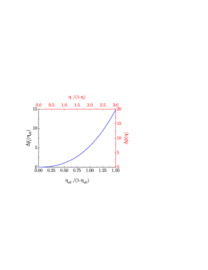
Figure 8: (Color online) Graphical illustration of the mapping “polydisperse mixture $\leftrightarrow$ pure fluid” defined by Eqs. (151) and (153). A common curve represents the EOS of the pure fluid (left and bottom axes) and that of the mixture (top and right axes). In this particular example the mixture is characterized by $m_{2}=\frac{3}{2}$ and $m_{3}=\frac{9}{2}$, so that $\lambda=2$ and $\omega=\frac{2}{3}$. A change in the composition of the mixture would only be reflected by a rescaling of the top and right axes. In this graph the curve corresponds to the single-component CS surplus pressure. Adapted from Fig. 1 of Ref. Santos et al., 2014.

From the thermodynamic relation $\Delta\widetilde{p}=\eta^{2}\partial\beta_{T}\Delta a/\partial\eta$, where the surplus pressure is defined in Eq. (131), Eq. (150) yields

$$\Delta\widetilde{p}_{\text{sp}}(\eta)=\lambda\omega\Delta\widetilde{p}_{\text{s}}(\eta_{\text{eff}}),$$ (153)

where we have used $\partial\eta_{\text{eff}}/\partial\eta=\lambda\eta_{\text{eff}}^{2}/\eta^{2}$. In terms of the compressibility factor, the mapping between the EOS of the monocomponent and multicomponent systems in the sp approximation becomes

$$Z_{\text{sp}}(\eta)=\frac{1}{1-\eta}+\lambda\omega\frac{\eta_{\text{eff}}}{\eta}\left[Z_{\text{s}}(\eta_{\text{eff}})-\frac{1}{1-\eta_{\text{eff}}}\right].$$ (154)

Since $\lambda\geq 1$ but $\omega\leq 1$, the product $\lambda\omega$ can be either larger or smaller than $1$, depending on the mixture composition. In the particular case of a binary mixture, it can be checked that $\lambda\omega>1$ only if the mole fraction of the small spheres is greater than a certain value, namely, $x_{1}>1/[1+(\sigma_{1}/\sigma_{2})^{3/2}]>\frac{1}{2}$.

The mapping defined by Eqs. (151) and (153) is illustrated by Fig. 8. A common curve describes both the multicomponent and the one-component systems, except that the top and right axes (corresponding to the mixture) are $\lambda$ and $\lambda\omega$ times, respectively, the bottom and left axes (corresponding to the pure fluid).

The e1–e3 and sp approximations can be formulated within a common framework in terms of the surplus pressure, as shown in the second column of Table 3. All of them share the consistency with the exact second and third virial coefficients. On the other hand, as stressed before, while in the e1–e3 approximations the EOS of the mixture is related to that of the monocomponent fluid evaluated at the same packing fraction, in the sp approximation the reference monocomponent fluid is evaluated at a different (effective) packing fraction $\eta_{\text{eff}}$. Interestingly, if the monocomponent SPT surplus pressure $\Delta\widetilde{p}_{\text{s}}(\eta)=3\eta^{2}/(1-\eta)^{3}$ is used, three of the four approximations (namely, e2, e3, and sp) yield the multicomponent SPT function $\Delta\widetilde{p}(\eta)=3\omega\eta^{2}[\eta+\lambda(1-\eta)]/\lambda^{2}(1-\eta)^{3}$. This proves the high degree of internal self-consistence of the SPT, even though it is not particularly accurate. On the other hand, if a better one-component EOS is used as input (for instance, $Z_{\text{s}}=Z_{\text{CS}}$), one finds $Z_{\text{e1}}(\eta)>Z_{\text{sp}}(\eta)>Z_{\text{e3}}(\eta)>Z_{\text{e2}}(\eta)$.

IV.5 Comparison with computer simulations

Table 3: Surplus pressure of the multicomponent system, $\Delta\widetilde{p}$, expressed in terms of the surplus pressure of the single-component fluid, $\Delta\widetilde{p}_{\text{s}}$, according to the approximations e1–e3 and sp. The third column gives the single-component compressibility factor, $Z_{\text{s}}$, as inferred from that of the mixture, $Z$. The parameters $\lambda$ and $\omega$ are defined in Eq. (143).

Approximation	$\Delta\widetilde{p}(\eta)$	$Z_{\text{s}}(\eta)$
e1	$\displaystyle{\frac{\omega(\lambda+1)}{2\lambda^{2}}\left[\Delta\widetilde{p}_{\text{s}}(\eta)+\frac{\lambda-1}{\lambda+1}\frac{3\eta^{2}}{1-\eta}\right]}$	$\displaystyle{\frac{1}{1-\eta}+\frac{2\lambda^{2}}{\omega(\lambda+1)}\left[Z(\eta)-\frac{1}{1-\eta}\right]-\frac{\lambda-1}{\lambda+1}\frac{3\eta}{1-\eta}}$
e2	$\displaystyle{\frac{\omega}{\lambda^{2}}\Delta\widetilde{p}_{\text{s}}(\eta)\left[\eta+\lambda(1-\eta)\right]}$	$\displaystyle{\frac{1}{1-\eta}+\frac{\lambda^{2}}{\omega}\frac{Z(\eta)-{1}/{(1-\eta)}}{\eta+\lambda(1-\eta)}}$
e3	$\displaystyle{\frac{\omega}{\lambda^{2}}\left[\Delta\widetilde{p}_{\text{s}}(\eta)+(\lambda-1)\frac{3\eta^{2}}{(1-\eta)^{2}}\right]}$	$\displaystyle{\frac{1}{1-\eta}+\frac{\lambda^{2}}{\omega}\left[Z(\eta)-\frac{1}{1-\eta}\right]-(\lambda-1)\frac{3\eta}{(1-\eta)^{2}}}$
sp	$\lambda\omega\Delta\widetilde{p}_{\text{s}}(\eta_{\text{eff}}),$ $\eta_{\text{eff}}\equiv\displaystyle{\frac{\eta}{\eta+\lambda(1-\eta)}}$	$\displaystyle{\frac{1}{1-\eta}+\frac{\eta_{\text{m}}/\eta}{\lambda\omega}\left[Z(\eta_{\text{m}})-\frac{1}{1-\eta_{\text{m}}}\right]}$, $\displaystyle{\eta_{\text{m}}\equiv\frac{\eta}{\eta+(1-\eta)/\lambda}}$

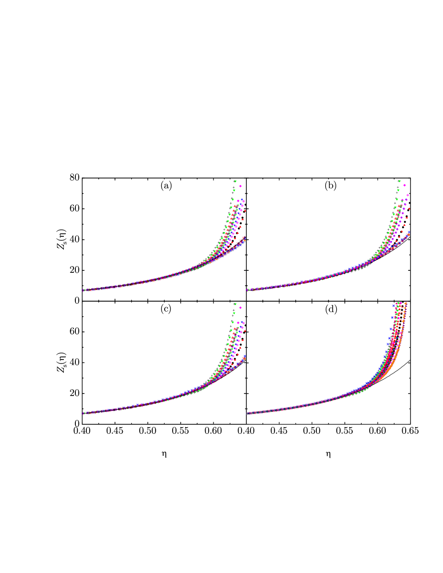
Figure 9: Plot of the monocomponent compressibility factor $Z_{\text{s}}(\eta)$, as inferred from simulation data for the mixtures described in Ref. Santos et al., 2014, according to the (a) e1, (b) e2, (c) e3, and (d) sp prescriptions. The solid lines represent the CS EOS [Eq. (II.2.3)]. Panel (d) is adapted from Fig. 2(b) of Ref. Santos et al., 2014.

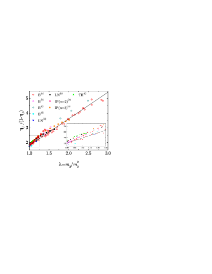
Figure 10: Test of the prediction for the jamming packing fraction of polydisperse HS mixtures as given by Eq. (155), here represented by the straight solid line. Several classes of size distribution are considered: binary (B), log-normal (LN), truncated inverse-power (IP), and top-hat (TH). The superscripts indicate the sources: (a) indicates experimental data from Ref. Yerazunis, Cornell, and Wintner, 1965, (b) indicates simulation data from Ref. Biazzo et al., 2009, (c) indicates simulation data from Ref. Hopkins, Stillinger, and Torquato, 2013, (d) indicates simulation data from Ref.  Desmond and Weeks, 2014, and (e) indicates simulation data from Refs. Ogarko and Luding, 2012, 2013; Santos et al., 2014. The inset is a magnifications of the framed region. Adapted from Fig. 3(a) of Ref. Santos et al., 2014.

It should be stressed that the proposals implied by Eqs. (118), (128), (136a), and (154) may be interpreted in two directions. On the one hand, if $Z_{\text{s}}$ is known as a function of the packing fraction, then one can readily compute the compressibility factor of the mixture for any packing fraction and composition [$\eta_{\text{eff}}$ and $\eta$ being related through Eq. (151) in the case of $Z_{\text{sp}}$]; this is the standard view. On the other hand, if simulation data for the EOS of the mixture are available for different densities, size ratios, and mole fractions, Eqs. (118), (128), (136a), and (154) can be used to infer the compressibility factor of the monocomponent fluid.Santos, Yuste, and López de Haro (2011); Santos et al. (2014) This is particularly important in the high-density region, where obtaining data from simulation may be accessible in the case of mixtures but either difficult or not feasible in the case of the monocomponent fluid, as that happens in the metastable fluid branch.Santos et al. (2017, 2014) The third column of Table 3 provides the expressions of the single-component fluid compressibility factor, as inferred from that of the multicomponent system, for the four approximations discussed in this section.

In principle, simulation data for different mixtures would yield different inferred functions $Z_{\text{s}}(\eta)$. Thus, without having to use an externally imposed monocomponent EOS, the degree of collapse of the mapping from mixture compressibility factors onto a common function $Z_{\text{s}}(\eta)$ is an efficient way of assessing the performance of Eqs. (118), (128), (136a), and (154). Let us test those mappings $Z\to Z_{\text{s}}$ by using simulation data corresponding to the mixtures described in Ref. Santos et al., 2014, namely, $6$ binary mixtures and $11$ polydisperse fluids with three classes of continuous size distributions (top-hat, truncated inverse-power, and log-normal) and the explored values of the parameters $\lambda$ and $\omega$ being $1.01\lesssim\lambda\lesssim 1.63$ and $0.61\lesssim\omega\lesssim 0.99$.

As shown in Figure 9, the usefulness of the mappings is confirmed by the nice collapse for all the points up to packing fractions below approximately the glass transition value $\eta_{\text{g}}\simeq 0.58$.Parisi and Zamponi (2010); Speedy (1998) This includes the metastable region beyond the freezing point ($\eta_{\text{f}}\simeq 0.492$), where simulation results for the monocomponent system are difficult to obtain.Odriozola and Berthier (2011) Beyond $\eta_{\text{g}}$, the collapse clearly fails in the e1–e3 inferences. On the other hand, the spread is significantly reduced in the case of the sp inference, although a certain degree of dispersion still remains, as expected from an algorithm-dependent out-of-equilibrium glass branch. This gives support to our expectation that the relationship implied by Eq. (154) (when extrapolated to metastable states) might be useful for inferring the EOS of a metastable pure HS fluid from the knowledge of the high-density behavior of polydisperse HS mixtures, which is much more accessible than in the monodisperse case.Odriozola and Berthier (2011)

As a consequence of their ability to attain higher packing fractions than the monocomponent system, the jamming packing fraction $\eta_{\text{J}}$ of a polydisperse HS system is typically higher than the jamming packing fraction (also called random close-packing fraction) $\eta_{\text{J,{\text{s}}}}$ of the one-component (monodisperse) system. Also, as that happens with $\eta_{\text{J,{\text{s}}}}$, the value of $\eta_{\text{J}}$ depends on the out-of-equilibrium compression protocol followed to jam the system.Parisi and Zamponi (2010); Biazzo et al. (2009) Apart from that, since $\eta_{\text{J}}$ is a functional of the full size distribution function $x(\sigma)$, it differs widely from system to system without an apparent unifying framework. It obviously would be desirable to have a way to characterize the whole distribution by a single “dispersity” parameter such that the actual values of $\eta_{\text{J}}$ for different polydisperse systems would tend to approximately fall on a “universal” curve when plotted against such a dispersity parameter. This would provide a tool to organize the apparently disconnected bunch of jamming packing values $\eta_{\text{J}}$ of different mixtures. We have shown that this is indeed possible.Santos et al. (2014) What we have done is to assume that Eqs. (151) and (154) are still valid (at least semiquantitatively) near the jamming point and take the value of $\lambda$ [see Eq. (143)] as the dispersity parameter (with the understanding that $\lambda=1$ defines the monodisperse case). Since one must have $\lim_{\eta\to\eta_{\text{J,{\text{s}}}}}Z_{\text{s}}(\eta)=\infty$ and $\lim_{\eta\to\eta_{\text{J}}}Z_{\text{sp}}(\eta)=\infty$, Eq. (151) implies that $\eta_{\text{J}}$ is such that its associated effective one-component value of $\eta_{\text{eff}}$ coincides with $\eta_{\text{J,{\text{s}}}}$. Hence, it follows that

$$\frac{\eta_{\text{J}}}{1-\eta_{\text{J}}}=\lambda\frac{\eta_{\text{J,{\text{s}}}}}{1-\eta_{\text{J,{\text{s}}}}},\quad\eta_{\text{J}}=\frac{\eta_{\text{J,{\text{s}}}}}{\eta_{\text{J,{\text{s}}}}+(1-\eta_{\text{J,{\text{s}}}})/\lambda}.$$ (155)

Equation (155) fulfills the requirement posed above. First, all the details of the size distribution function $x(\sigma)$ are encapsulated in the moment ratio $\lambda=m_{3}/m_{2}^{2}$, which then plays the role of the sought dispersity parameter. Secondly, the functional form $\eta_{\text{J}}(\lambda)$ is quite simple: the occupied/void volume ratio at jamming, i.e., ${\eta_{\text{J}}}/({1-\eta_{\text{J}}})$, is just proportional to $\lambda$ with the slope being given by the monocomponent value. Prediction (155) is favorably tested against experimentalYerazunis, Cornell, and Wintner (1965) and simulationBiazzo et al. (2009); Ogarko and Luding (2012, 2013); Hopkins, Stillinger, and Torquato (2013); Desmond and Weeks (2014); Santos et al. (2014) data in Fig. 10 taking $\eta_{\text{J,{\text{s}}}}=0.644$.Biazzo et al. (2009)

V Concluding Remarks

In this paper we have attempted to provide a self-contained account of some of our (almost completely analytical) efforts over the past three decades in the study of the thermodynamic and structural properties of HS systems which have catered for, whenever possible, the consideration of mixtures with an arbitrary number of components (including polydisperse systems). These efforts include the RFA formalism, which is certainly an alternative methodology to the usual integral equation approach employed in liquid-state theory to obtain the structural properties of HS fluids. Using this formalism, we have been able to obtain explicit analytical or semi-analytical results for the RDF, the DCF, the static structure factor, and the bridge functions, in the end requiring as input only the contact value of the RDF of the single-component or multicomponent HS fluid. One of the nice assets of the RFA is that, by construction, it eliminates the thermodynamic consistency problem which is present in most of the integral equation formulations for the computation of structural quantities. Moreover, this formalism has been amply shown to certainly improve the agreement between theory and computer simulation results in comparison, say, to both the PY and HNC approximations. Very recently, for instance, we have also used the RFA to investigate the long-range behavior of the structural correlation functions, including the feature of structural crossover, in binary mixtures of additive HS.Pieprzyk et al. (2020)

The RFA methodology can be applied beyond three-dimensional HS systems. Those systems can be classified into two categories: (i) those that admit an exact solution of the PY integral equation and (ii) those that are not exactly solvable within the PY approximation. In the first class of systems, the RFA method not only recovers, on the one hand, and improves, on the other hand, the PY solution for three-dimensional single-component or multicomponent HS fluids, but also does for hard hyperspheresRohrmann and Santos (2007, 2011a, 2011b) and three-dimensional sticky-hard-sphere systems.Yuste and Santos (1993); Santos, Yuste, and López de Haro (1998); Yuste, Santos, and López de Haro (2008). The application of RFA-like approaches to systems of the second class (i.e., those lacking an exact PY solution) includes the penetrable-sphere model,Malijevský and Santos (2006); Malijevský, Yuste, and Santos (2007) the penetrable-square-well model,Fantoni et al. (2009) the square-well and square-shoulder potentials,Yuste and Santos (1994); Acedo and Santos (2001); Largo et al. (2005); Yuste, Santos, and López de Haro (2011); López de Haro, Yuste, and Santos (2016), piecewise-constant potentials with several steps,Santos, Yuste, and López de Haro (2012); Santos et al. (2013); López de Haro et al. (2018) nonadditive HS mictures,Fantoni and Santos (2011, 2013, 2014), and Janus particles with constrained orientations.Maestre et al. (2013) In those cases, the simplest RFA is already quite accurate, generally improving on the (numerical) solution of the PY approximation. Moreover, the RFA is also directly applicable within the thermodynamic perturbation approach to the computation of the properties of real fluids.

The other area in which we have put attention here, where our work has also produced some interesting results, is the one pertaining to the EOS of HS mixtures. In this case, starting from relatively simple but otherwise reasonable assumptions whose merits may be judged a posteriori, we have made use of some exact consistency conditions to devise various approximate proposals that extend any given single-component EOS to multicomponent fluid mixtures with any composition and which are in good agreement with simulation results. Some noteworthy aspects of the results that follow from these developments were illustrated here through the prediction of the jamming packing-fraction of multicomponent systems as a simple function of a quantity involving the first three moments of the size distribution. We should also mention that the ideas presented here in connection with the EOS for additive multicomponent HS mixtures have also been used for nonadditive systems and for hard-hypersphere systems with arbitrary spatial dimensions.González-Melchor, Alejandre, and López de Haro (2001); Santos, López de Haro, and Yuste (2005); López de Haro, Yuste, and Santos (2008); Santos, López de Haro, and Yuste (2010); Fiumara et al. (2017); López de Haro, Santos, and Yuste (2020)

Finally, it should be clear that there are many facets of the equilibrium and structural properties of many other hard-core systems that may be studied following the ideas presented here but that up to now have not been considered. For instance, the generalization of the RFA approach to square-well or square-shoulder mixtures and the surplus mapping of the single-component EOS to that of nonadditive HS mixtures appear as interesting challenges. We hope to address some of these problems in the future and would be very much rewarded if some others were taken up by researchers who might find these developments also a valuable tool for their work.

Appendix A On the functional forms of $\widetilde{h}(q)$ and $\widetilde{c}(q)$

In this appendix we present the expected functional forms of the correlation functions $\widetilde{h}(q)$ and $\widetilde{c}(q)$ in terms of an auxiliary function related to the Laplace transform $G(s)$ defined by Eq. (62).

For simplicity, we choose here $\sigma=1$ as the length unit. Let us define $\widehat{F}(s)\equiv\left[{2\pi\Psi(s)}\right]^{-1}$ and rewrite Eqs. (64) and (70) as

$$G(s)=s\frac{\widehat{F}(s)e^{-s}}{1+12\eta\widehat{F}(s)e^{-s}},$$ (156a)

$$G(s)=s\sum_{n=1}^{\infty}(-12\eta)^{n-1}\left[F(s)\right]^{n}e^{-ns}.$$ (156b)

The small-$s$ behavior (69) translates into

$$\frac{e^{s}}{\widehat{F}(s)}=-12\eta+s^{3}+\mathcal{O}(s^{5}).$$ (157)

On the other hand, the large-$s$ behavior is

$$\widehat{F}(s)=\frac{\widehat{F}_{2}}{s^{2}}+\frac{\widehat{F}_{3}}{s^{3}}+\frac{\widehat{F}_{4}}{s^{4}}+\frac{\widehat{F}_{5}}{s^{5}}+\cdots,$$ (158a)

$$\widehat{F}_{n}= \lim_{r\to 1^{+}}\frac{\partial^{n-2}}{\partial r^{n-2}}\left[rg(r)\right]$$

$$= (n-2)\bar{g}^{(n-3)}+\bar{g}^{(n-2)}.$$ (158b)

This extends Eq. (67) to higher-order terms. In Eq. (158), $\bar{g}^{(n)}\equiv\lim_{r\to 1^{+}}\partial^{n}g(r)/\partial r^{n}$.

Let us now insert Eqs. (156) into Eq. (III.1.1) to get

$$\widetilde{h}(q)=-2\pi\frac{\widehat{F}(\imath q)e^{-\imath q}+\widehat{F}(-\imath q)e^{\imath q}+24\eta\widehat{F}(\imath q)\widehat{F}(-\imath q)}{1+12\eta\widehat{F}(\imath q)e^{-\imath q}+12\eta\widehat{F}(-\imath q)e^{\imath q}+144\eta^{2}\widehat{F}(\imath q)\widehat{F}(-\imath q)},$$ (159a)

$$\widetilde{h}(q)=\sum_{n=1}^{\infty}\left[C^{(n)}(q)\cos(nq)+D^{(n)}(q)\sin(nq)\right].$$ (159b)

In Eq. (159b),

$$C^{(n)}(q)=-2\pi(-12\eta)^{n-1}\left\{\left[\widehat{F}(\imath q)\right]^{n}+\left[\widehat{F}(-\imath q)\right]^{n}\right\},$$ (160a)

$$D^{(n)}(q)=2\pi(-12\eta)^{n-1}\imath\left\{\left[\widehat{F}(\imath q)\right]^{n}-\left[\widehat{F}(-\imath q)\right]^{n}\right\}.$$ (160b)

Taking into account the expansion (158a), one can write

$$\left[\widehat{F}(s)\right]^{n}= \frac{1}{s^{2n}}\left(\widehat{F}_{2}+\frac{\widehat{F}_{3}}{s}+\frac{\widehat{F}_{4}}{s^{2}}+\cdots\right)^{n}$$

$$= \frac{\widehat{F}_{2}^{n}}{s^{2n}}\left[1+\frac{n\widehat{F}_{3}}{\widehat{F}_{2}s}+n\frac{(n-1)\widehat{F}_{3}^{2}+2\widehat{F}_{2}\widehat{F}_{4}}{2\widehat{F}_{2}^{2}s^{2}}+\cdots\right],$$ (161a)

$$C^{(n)}(q)= 4\pi(12\eta)^{n-1}\frac{\widehat{F}_{2}^{n}}{q^{2n}}$$

$$\times\left[1-n\frac{(n-1)\widehat{F}_{3}^{2}+2\widehat{F}_{2}\widehat{F}_{4}}{2\widehat{F}_{2}^{2}q^{2}}+\mathcal{O}(q^{-4})\right],$$ (161b)

$$D^{(n)}(q)=-4\pi(12\eta)^{n-1}\frac{\widehat{F}_{2}^{n}}{q^{2n}}\left[\frac{n\widehat{F}_{3}}{\widehat{F}_{2}q}+\mathcal{O}(q^{-3})\right].$$ (161c)

Therefore, the large-$q$ structure of $C^{(n)}(q)$ and $D^{(n)}(q)$ is

$$C^{(n)}(q)=\sum_{m=n}^{\infty}\frac{C^{(n)}_{m}}{q^{2m}},$$ (162a)

$$D^{(n)}(q)=\sum_{m=n}^{\infty}\frac{D^{(n)}_{m}}{q^{2m+1}}.$$ (162b)

In particular,

$$C^{(1)}_{m}=-4\pi(-1)^{m}\widehat{F}_{2m},$$ (163a)

$$D^{(1)}_{m}=4\pi(-1)^{m}\widehat{F}_{2m+1},$$ (163b)

$$C^{(n)}_{n}=4\pi(12\eta)^{n-1}\widehat{F}_{2}^{n},$$ (163c)

$$C^{(n)}_{n+1}=-2\pi(12\eta)^{n-1}n\widehat{F}_{2}^{n-2}\left[(n-1)\widehat{F}_{3}^{2}+2\widehat{F}_{2}\widehat{F}_{4}\right],$$ (163d)

$$D^{(n)}_{n}=-4\pi(12\eta)^{n-1}n\widehat{F}_{2}^{n-1}\widehat{F}_{3}.$$ (163e)

It is worth noticing that the structure of Eqs. (159b) and (162) agrees with that of Eq. (9) of Ref. Pieprzyk, Brańka, and Heyes, 2017 only if the terms with $n>1$ in Eq. (159b) are ignored. On the other hand, the coefficients $C^{(1)}_{1}$, $C^{(1)}_{2}$, $D^{(1)}_{1}$, and $D^{(1)}_{2}$, as given by Eqs. (158) and (163), agree with Eqs. (10)–(11) of Ref. Pieprzyk, Brańka, and Heyes, 2017.

Let us consider now the DCF. It can be obtained in Fourier space by insertion of Eq. (159a) into the OZ relation (19). The result is

$$\widetilde{c}(q)= -{2\pi}\frac{\widehat{F}(\imath q)e^{-\imath q}+\widehat{F}(-\imath q)e^{\imath q}+24\eta\widehat{F}(\imath q)\widehat{F}(-\imath q)}{1-144\eta^{2}\widehat{F}(\imath q)\widehat{F}(-\imath q)}$$

$$= \bar{C}^{(0)}(q)+\bar{C}^{(1)}(q)\cos q+\bar{D}^{(1)}(q)\sin q,$$ (164)

with

$$\bar{C}^{(0)}=-48\pi\eta\frac{\widehat{F}(\imath q)\widehat{F}(-\imath q)}{1-144\eta^{2}\widehat{F}(\imath q)\widehat{F}(-\imath q)},$$ (165a)

$$\bar{C}^{(1)}=-2\pi\frac{\widehat{F}(\imath q)+\widehat{F}(-\imath q)}{1-144\eta^{2}\widehat{F}(\imath q)\widehat{F}(-\imath q)},$$ (165b)

$$\bar{D}^{(1)}=2\pi\imath\frac{\widehat{F}(\imath q)-\widehat{F}(-\imath q)}{1-144\eta^{2}\widehat{F}(\imath q)\widehat{F}(-\imath q)}.$$ (165c)

Equations (159b) and (A) are formally exact and express the Fourier transforms $\widetilde{h}(q)$ and $\widetilde{c}(q)$ in terms of the (unknown) function $\widehat{F}(s)$ [see Eq. (156a)] evaluated at $s=\pm\imath q$. In the special case that $\widehat{F}(s)$ is an algebraic function, all the singularities of $h(r)$ occur at $r=n$ and the only singularity of $c(r)$ takes place at $r=1$.

Appendix B Expressions for the amplitudes in Eq. (III.1.3)

The explicit expressions for the amplitudes $K_{\pm}$, $K_{-1}$, $K_{0}$, $K_{1}$, $K_{3}$, and $K$ appearing in Eq. (III.1.3) are

$$K_{\pm}= \frac{e^{\mp\kappa}}{\alpha^{2}(1-\eta)^{4}\kappa^{6}}\Bigl{\{}1+2(1+3\alpha)\eta\pm\left[1+\frac{\eta}{2}+\alpha(1+2\eta)\right]\kappa+\frac{1-\eta}{2}\left[\kappa^{2}-\eta\left(12+(\kappa\pm 6)\kappa\right)\right]\frac{L^{(2)}}{\pi}\Big{\}}$$

$$\times\Bigl{\{}6\eta\left[1+2(1+3\alpha)\eta\right]\pm 3\eta\left[3\eta-2\alpha(1-4\eta)\right]\kappa-3\eta(1+2\alpha)(1-\eta)\kappa^{2}-\frac{(1-\eta)^{2}}{2}\kappa^{3}(\alpha\kappa\mp 1)$$

$$+3\eta(1-\eta)\left[\kappa^{2}-\eta\left(12+(\kappa\pm 6)\kappa\right)\right]\frac{L^{(2)}}{\pi}\Big{\}},$$ (166a)

$$K_{-1}=-\left[\frac{L^{(2)}}{2\pi\alpha}+K_{+}e^{\kappa}+K_{-}e^{-\kappa}+K_{0}+K_{1}+K_{3}\right],$$ (166b)

$$K_{0}=-\left[\frac{1+2\left(1+3\alpha\right)\eta-6\eta\left(1-\eta\right)L^{(2)}/\pi}{\alpha\kappa\left(1-\eta\right)^{2}}\right]^{2},$$ (166c)

$$K_{1}= \frac{6\eta}{\kappa^{2}}K_{0}+\frac{6\eta}{\alpha^{2}\kappa^{2}\left(1-\eta\right)^{4}}\Big{\{}\left[1+\frac{\eta}{2}+\alpha(1+2\eta)\right]^{2}$$

$$-\left(1-\eta\right)\left[1+\eta(7+\eta+6\alpha\left(2+\eta\right))\right]\frac{L^{(2)}}{\pi}$$

$$+3\eta\left(2+\eta\right)(1-\eta)^{2}\frac{{L^{(2)}}^{2}}{\pi^{2}}\Big{\}},$$ (166d)

$$K_{3}=\frac{\eta}{2}K_{0},$$ (166e)

$$K=-\left(K_{+}+K_{-}+K_{-1}\right).$$ (166f)

Here we have again taken $\sigma=1$ as the length unit.

DATA AVAILABILITY

The data that support the findings of this study are available from the corresponding author upon reasonable request.

REFERENCES

REFERENCES

- Barker and Henderson (1976) J. A. Barker and D. Henderson, “What is “liquid”? Understanding the states of matter,” Rev. Mod. Phys. 48, 587–671 (1976).
- McQuarrie (1976) D. A. McQuarrie, Statistical Mechanics (Harper & Row, New York, 1976).
- Friedman (1985) H. L. Friedman, A Course in Statistical Mechanics (PrenticeHall, Englewood Cliffs, 1985).
- Hansen and McDonald (2006) J.-P. Hansen and I. R. McDonald, Theory of Simple Liquids, 3rd ed. (Academic, London, 2006).
- Solana (2013) J. R. Solana, Perturbation Theories for the Thermodynamic Properties of Fluids and Solids (CRC Press, Boca Raton, 2013).
- Thiesen (1885) M. Thiesen, “Untersuchungen über die Zustandsgleichung,” Ann. der Phys. 260, 467–492 (1885).
- Kamerlingh Onnes (1901) H. Kamerlingh Onnes, “Expression of the equation of state of gases and liquids by means of series,” Commun. Phys. Lab. Univ. Leiden 71, 3–25 (1901), reprinted in Expression of the equation of state of gases and liquids by means of series in Through Measurement to Knowledge, Boston Studies in the Philosophy and History of Science, Vol. 124, (Springer Netherlands, 1991), pp. 146–163.
- Mayer and Goeppert Mayer (1940) J. E. Mayer and M. Goeppert Mayer, Statistical Mechanics (Wiley, New York, 1940).
- Masters (2008) A. J. Masters, “Virial expansions,” J. Phys.: Condens. Matter 20, 283102 (2008).
- Hoover and Hoover (2020) W. G. Hoover and C. G. Hoover, “From hard spheres and cubes to nonequilibrium maps with thirty-some years of thermostatted molecular dynamics,” J. Chem. Phys. 153, 070901 (2020).
- Santos (2016) A. Santos, A Concise Course on the Theory of Classical Liquids. Basics and Selected Topics, Lecture Notes in Physics, Vol. 923 (Springer, New York, 2016).
- Santos (2012a) A. Santos, “Chemical-potential route: A hidden Percus–Yevick equation of state for hard spheres,” Phys. Rev. Lett. 109, 120601 (2012a).
- Santos and Rohrmann (2013) A. Santos and R. D. Rohrmann, “Chemical-potential route for multicomponent fluids,” Phys. Rev. E 87, 052138 (2013).
- Ashcroft and Langreth (1967) N. W. Ashcroft and D. C. Langreth, “Structure of binary liquid mixtures. I,” Phys. Rev. 156, 685–692 (1967).
- Bhatia and Thornton (1970) A. B. Bhatia and D. E. Thornton, “Structural aspects of the electrical resistivity of binary alloys,” Phys. Rev. B 2, 3004–3012 (1970).
- Morita (1958) T. Morita, “Theory of classical fluids: Hyper-netted chain approximation, I: : Formulation for a one-component system,” Prog. Theor. Phys. 20, 920–938 (1958).
- Morita (1960) T. Morita, “Theory of classical fluids: Hyper-netted chain approximation. III: A new integral equation for the pair distribution function,” Prog. Theor. Phys. 23, 829–845 (1960).
- van Leeuwen, Groeneveld, and de Boer (1959) J. M. J. van Leeuwen, J. Groeneveld, and J. de Boer, “New method for the calculation of the pair correlation function. I,” Physica 25, 792–808 (1959).
- Percus and Yevick (1958) J. K. Percus and G. J. Yevick, “Analysis of classical statistical mechanics by means of collective coordinates,” Phys. Rev. 110, 1–13 (1958).
- Santos and Manzano (2010) A. Santos and G. Manzano, “Simple relationship between the virial-route hypernetted-chain and the compressibility-route Percus–Yevick values of the fourth virial coefficient,” J. Chem. Phys. 132, 144508 (2010).
- Verlet (1980) L. Verlet, “Integral equations for classical fluids I. The hard sphere case,” Mol. Phys. 41, 183–190 (1980).
- Verlet (1981) L. Verlet, “Integral equations for classical fluids II. Hard spheres again,” Mol. Phys. 42, 1291–1302 (1981).
- Martynov and Sarkisov (1983) G. A. Martynov and G. N. Sarkisov, “Exact equations and the theory of liquids. V,” Mol. Phys. 49, 1495–1504 (1983).
- Rogers and Young (1984) F. J. Rogers and D. A. Young, “New, thermodynamically consistent, integral equation for simple fluids,” Phys. Rev. A 30, 999–1007 (1984).
- Ballone et al. (1986) P. Ballone, G. Pastore, G. Galli, and D. Gazzillo, “Additive and non-additive hard sphere mixtures. Monte Carlo simulation and integral equation results,” Mol. Phys. 59, 275–290 (1986).
- Santos, Fantoni, and Giacometti (2009) A. Santos, R. Fantoni, and A. Giacometti, “Thermodynamic consistency of energy and virial routes: An exact proof within the linearized Debye–Hückel theory,” J. Chem. Phys. 131, 181105 (2009).
- Santos (2007) A. Santos, “Thermodynamic consistency between the energy and virial routes in the mean spherical approximation for soft potentials,” J. Chem. Phys. 126, 116101 (2007).
- Mulero (2008) A. Mulero, ed., Theory and Simulation of Hard-Sphere Fluids and Related Systems, Lecture Notes in Physics, Vol. 753 (Springer, Berlin, 2008).
- Santos (2005) A. Santos, “On the equivalence between the energy and virial routes to the equation of state of hard-sphere fluids,” J. Chem. Phys. 123, 104102 (2005).
- Santos (2006) A. Santos, “Are the energy and virial routes to thermodynamics equivalent for hard spheres?” Mol. Phys. 104, 3411–3418 (2006).
- Nairn and Kilpatrick (1972) J. H. Nairn and J. E. Kilpatrick, “van der Waals, Boltzmann, and the fourth virial coefficient of hard spheres,” Am. J. Phys. 40, 503–515 (1972).
- Labík, Kolafa, and Malijevský (2005) S. Labík, J. Kolafa, and A. Malijevský, “Virial coefficients of hard spheres and hard disks up to the ninth,” Phys. Rev. E 71, 021105 (2005).
- Clisby and McCoy (2006) N. Clisby and B. M. McCoy, “Ninth and tenth order virial coefficients for hard spheres in dimensions,” J. Stat. Phys. 122, 15–57 (2006).
- Wheatley (2013) R. J. Wheatley, “Calculation of high-order virial coefficients with applications to hard and soft spheres,” Phys. Rev. Lett. 110, 200601 (2013).
- McCoy (2010) B. M. McCoy, Advanced Statistical Mechanics (Oxford University Press, Oxford, UK, 2010).
- Lebowitz and Penrose (1964) J. L. Lebowitz and O. Penrose, “Convergence of virial expansions,” J. Math. Phys. 5, 841–847 (1964).
- Procacci and Scoppola (2007) R. F. A. Procacci and B. Scoppola, “The analyticity region of the hard sphere gas. improved bounds,” J. Stat. Phys. 128, 1139–1143 (2007).
- Rohrmann et al. (2008) R. D. Rohrmann, M. Robles, M. López de Haro, and A. Santos, “Virial series for fluids of hard hyperspheres in odd dimensions,” J. Chem. Phys. 129, 014510 (2008).
- Adda-Bedia, Katzav, and Vella (2008) M. Adda-Bedia, E. Katzav, and D. Vella, “Solution of the Percus–Yevick equation for hard hyperspheres in even dimensions,” J. Chem. Phys. 129, 144506 (2008).
- Nijboer and van Hove (1952) B. R. A. Nijboer and L. van Hove, “Radial distribution function of a gas of hard spheres and the superposition approximation,” Phys. Rev. 85, 777–783 (1952).
- Ree, Keeler, and McCarthy (1966) F. H. Ree, R. N. Keeler, and S. L. McCarthy, “Radial distribution function of hard spheres,” J. Chem. Phys. 44, 3407–3425 (1966).
- Santos and Malijevský (2007) A. Santos and A. Malijevský, “Radial distribution function of penetrable sphere fluids to the second order in density,” Phys. Rev. E 75, 021201 (2007).
- Thiele (1963) E. Thiele, “Equation of state for hard spheres,” J. Chem. Phys. 39, 474–479 (1963).
- Wertheim (1963) M. S. Wertheim, “Exact solution of the Percus–Yevick integral equation for hard spheres,” Phys. Rev. Lett. 10, 321–323 (1963).
- Wertheim (1964) M. S. Wertheim, “Analytic solution of the Percus–Yevick equation,” J. Math. Phys. 5, 643–651 (1964).
- Ashcroft and Lekner (1966) N. W. Ashcroft and J. Lekner, “Structure and resistivity of liquid metals,” Phys. Rev. 145, 83–90 (1966).
- Lebowitz (1964) J. L. Lebowitz, “Exact solution of generalized Percus–Yevick equation for a mixture of hard spheres,” Phys. Rev. 133, A895–A899 (1964).
- Lebowitz and Zomick (1971) J. L. Lebowitz and D. Zomick, “Mixtures of hard spheres with nonadditive diameters: Some exact results and solution of PY equation,” J. Chem. Phys. 54, 3335–3346 (1971).
- Carnahan and Starling (1969) N. F. Carnahan and K. E. Starling, “Equation of state for nonattracting rigid spheres,” J. Chem. Phys. 51, 635–636 (1969).
- Boublík and Nezbeda (1986) T. Boublík and I. Nezbeda, “P-V-T behaviour of hard body fluids. theory and experiment,” Collect. Czech. Chem. Commun. 51, 2301–2432 (1986).
- Baus and Colot (1987) M. Baus and J. L. Colot, “Thermodynamics and structure of a fluid of hard rods, disks, spheres, or hyperspheres from rescaled virial expansions,” Phys. Rev. A 36, 3912–3925 (1987).
- Mulero et al. (2008) A. Mulero, C. A. Galán, M. I. Parra, and F. Cuadros, “Equations of State for Hard Spheres and Hard Disks,” in Theory and Simulation of Hard-Sphere Fluids and Related Systems, Lecture Notes in Physics, Vol. 753, edited by A. Mulero (Springer-Verlag, Berlin, 2008) pp. 37–109.
- Guerrero and Bassi (2008) A. O. Guerrero and A. B. M. S. Bassi, “On Padé approximants to virial series,” J. Chem. Phys. 129, 044509 (2008).
- Pieprzyk et al. (2019) S. Pieprzyk, M. N. Bannerman, A. C. Brańka, M. Chudak, and D. M. Heyes, “Thermodynamic and dynamical properties of the hard sphere system revisited by molecular dynamics simulation,” Phys. Chem. Chem. Phys. 21, 6886–6899 (2019).
- Tian, Jiang, and Mulero (2019) J. Tian, H. Jiang, and A. Mulero, “Equations of the state of hard sphere fluids based on recent accurate virial coefficients –,” Phys. Chem. Chem. Phys. 21, 13070–13077 (2019).
- Kolafa, Labík, and Malijevský (2004) J. Kolafa, S. Labík, and A. Malijevský, “Accurate equation of state of the hard sphere fluid in stable and metastable regions,” Phys. Chem. Chem. Phys. 6, 2335–2340 (2004), see also http://www.vscht.cz/fch/software/hsmd/.
- Santos and López de Haro (2009) A. Santos and M. López de Haro, “A branch-point approximant for the equation of state of hard spheres,” J. Chem. Phys. 130, 214104 (2009).
- Freasier and Isbister (1981) B. C. Freasier and D. J. Isbister, “A remark on the Percus–Yevick approximation in high dimensions. Hard core systems,” Mol. Phys. 42, 927–936 (1981).
- Leutheusser (1984) E. Leutheusser, “Exact solution of the Percus–Yevick equation for a hard-core fluid in odd dimensions,” Physica A 127, 667–676 (1984).
- González, González, and Silbert (1990) D. J. González, L. E. González, and M. Silbert, “Thermodynamics of a fluid of hard -dimensional spheres: Percus-Yevick and Carnahan-Starling-like results for and ,” Phys. Chem. Liq. 22, 95–102 (1990).
- Bishop, Masters, and Clarke (1999) M. Bishop, A. Masters, and J. H. R. Clarke, “Equation of state of hard and Weeks–Chandle–Anderson hyperspheres in four and five dimensions,” J. Chem. Phys. 110, 11449–11453 (1999).
- Rohrmann and Santos (2007) R. D. Rohrmann and A. Santos, “Structure of hard-hypersphere fluids in odd dimensions,” Phys. Rev. E 76, 051202 (2007).
- Heyes and Santos (2016) D. M. Heyes and A. Santos, “Chemical potential of a test hard sphere of variable size in a hard-sphere fluid,” J. Chem. Phys. 145, 214504 (2016).
- Heyes and Santos (2018) D. M. Heyes and A. Santos, “Chemical potential of a test hard sphere of variable sizein hard-sphere fluid mixtures,” J. Chem. Phys. 148, 214503 (2018).
- Barošová et al. (1996) M. Barošová, A. Malijevský, S. Labík, and W. R. Smith, “Computer simulation of the chemical potentials of binary hard-sphere mixtures,” Mol. Phys. 87, 423–439 (1996).
- Boublík (1970) T. Boublík, “Hard-sphere equation of state,” J. Chem. Phys. 53, 471–472 (1970).
- Mansoori et al. (1971) G. A. Mansoori, N. F. Carnahan, K. E. Starling, and T. W. Leland, Jr., “Equilibrium thermodynamic properties of the mixture of hard spheres,” J. Chem. Phys. 54, 1523–1525 (1971).
- Alder and Wainwright (1957) B. J. Alder and T. E. Wainwright, “Phase transition for a hard sphere system,” J. Chem. Phys. 27, 1208–1209 (1957).
- Fernández et al. (2012) L. A. Fernández, V. Martín-Mayor, B. Seoane, and P. Verrocchio, “Equilibrium fluid-solid coexistence of hard spheres,” Phys. Rev. Lett. 108, 165701 (2012).
- Hoover and Ree (1968) W. G. Hoover and F. H. Ree, “Melting transition and communal entropy for hard spheres,” J. Chem. Phys. 49, 3609–3617 (1968).
- Speedy (1998) R. J. Speedy, “The hard sphere glass transition,” Mol. Phys. 95, 169–178 (1998).
- Torquato (2018) S. Torquato, “Perspective: Basic understanding of condensed phases of matter via packing models,” J. Chem. Phys. 149, 020901 (2018).
- van Megen and Underwood (1993) W. van Megen and S. M. Underwood, “Change in crystallization mechanism at the glass transition of colloidal spheres,” Nature 362, 616–618 (1993).
- van Blaaderen and Wiltzius (1995) A. van Blaaderen and P. Wiltzius, “Real-space structure of colloidal hard-sphere glasses,” Science 270, 1177–1179 (1995).
- Speedy (1994) R. J. Speedy, “On the reproducibility of glasses,” J. Chem. Phys. 100, 6684–6691 (1994).
- Yeo (1995) J. Yeo, “Metastable dynamics of the hard-sphere system,” Phys. Rev. E 52, 853–861 (1995).
- Aguilera-Navarro et al. (1984) V. C. Aguilera-Navarro, M. Fortes, M. de Llano, and O. Rojo, “May low-density expansions for imperfect gases contain information about condensed phases?” J. Chem. Phys. 81, 1450–1454 (1984).
- Gaunt and Joyce (1980) D. S. Gaunt and G. S. Joyce, “Virial expansions for hard-core fluids,” J. Phys. A: Math. Gen. 13, L211–L216 (1980).
- Joyce (1988) G. S. Joyce, “On the hard-hexagon model and the theory of modular functions,” Phil. Trans. Roy. Soc. A 325, 643–702 (1988).
- Baxter, Enting, and Tsang (1980) R. J. Baxter, I. G. Enting, and S. K. Tsang, “Hard-square lattice gas,” J. Stat. Phys. 22, 465–489 (1980).
- Sanchez (1994) I. C. Sanchez, “Virial coefficients and close–packing of hard spheres and disks,” J. Chem. Phys. 101, 7003–7006 (1994).
- Woodcock (1976) L. V. Woodcock, “Glass transition in the hard-sphere model,” J. Chem. Soc. Faraday Trans. 2 72, 1667–1672 (1976).
- Andrews (1975) F. C. Andrews, “Simple approach to the equilibrium statistical mechanics of the hard sphere fluid,” J. Chem. Phys. 62, 272–275 (1975).
- Andrews (1976) F. C. Andrews, “A simple approach to the equilibrium statistical mechanics of two-dimensional fluids,” J. Chem. Phys. 64, 1941–1947 (1976).
- Baram and Luban (1979) A. Baram and M. Luban, “Divergence of the virial series for hard discs and hard spheres at closest packing,” J. Phys. C 12, L659–L664 (1979).
- Devore and Schneider (1982) J. A. Devore and E. Schneider, “Equations of state for rigid disks and spheres,” J. Chem. Phys. 77, 1067–1068 (1982).
- Aguilera-Navarro et al. (1983) V. C. Aguilera-Navarro, M. Fortes, M. de Llano, A. Plastino, J. del Río, and O. Rojo, “Hard-sphere fluid-to-solid transition and the virial expansion,” J. Stat. Phys. 32, 95–104 (1983).
- Hoste and Van Dael (1984) R. Hoste and W. Van Dael, “Equation of state for hard-sphere and hard-disc systems,” J. Chem. Soc. Faraday Trans. 2 80, 477–488 (1984).
- Goldman and White (1988) J. I. Goldman and J. A. White, “Equation of state for the hard-sphere gas,” J. Chem. Phys. 89, 6403–6405 (1988).
- Wang, Mead, and de Llano (1991) D. Wang, L. R. Mead, and M. de Llano, “Maximum-entropy approach to classical hard-sphere and hard-disk equations of state,” J. Math. Phys. 32, 2258–2262 (1991).
- Santos, López de Haro, and Yuste (1995) A. Santos, M. López de Haro, and S. B. Yuste, “An accurate and simple equation of state for hard disks,” J. Chem. Phys. 103, 4622–4625 (1995).
- López de Haro, Santos, and Yuste (1998) M. López de Haro, A. Santos, and S. B. Yuste, “A student-oriented derivation of a reliable equation of state for a hard-disc fluid,” Eur. J. Phys. 19, 281–286 (1998).
- Wang, Khoshkbarchi, and Vera (1996) W. Wang, M. K. Khoshkbarchi, and J. H. Vera, “A new volume dependence for the equations of state of hard spheres,” Fluid Phase Equil. 115, 25–38 (1996).
- Khoshkbarchi and Vera (1997) M. K. Khoshkbarchi and J. H. Vera, “A simplified hard-sphere equation of state meeting the high and low density limits,” Fluid Phase Equil. 130, 189–194 (1997).
- Nasrifar, Ayatollahi, and Moshfeghian (2000) K. Nasrifar, S. Ayatollahi, and M. Moshfeghian, “Improving the simplified-perturbed-hard-chain theory equation of state using a new non-attracting hard-sphere equation,” Can. J. Chem. Eng. 78, 1111–1119 (2000).
- Ghotbi and Vera (2001) C. Ghotbi and J. H. Vera, “Extension to mixtures of two robust hard-sphere equations of state satisfying the ordered close-packed limit,” Can. J. Chem. Eng. 79, 678–686 (2001).
- Wang (2002) X. Z. Wang, “van der Waals–Tonks-type equations of state for hard-disk and hard-sphere fluids,” Phys. Rev. E 66, 031203 (2002).
- Polishuk and Vera (2005) I. Polishuk and J. H. Vera, “A novel equation of state for the prediction of thermodynamic properties of fluids,” J. Phys. Chem. B 109, 5977–5984 (2005).
- Miandehy, Modarress, and Dehghani (2006) M. Miandehy, H. Modarress, and M. R. Dehghani, “Equation of state for hard-spheres and excess function calculations of binary liquid mixtures,” Fluid Phase Equil. 239, 91–99 (2006).
- Korteweg (1892) D. I. Korteweg, “On Van der Waals’s isothermal equation,” Nature 45, 277–277 (1892).
- Boltzmann (1898) L. Boltzmann, Vorlesungen über Gastheorie (Barth, Leipzig, Germany, 1898) translated by S. G. Brush, Lectures on Gas Theory, part 2, Ch. 5 (University of California Press, Berkeley, CA, 1964).
- Le Fevre (1972) E. J. Le Fevre, “Equation of state for hard-sphere fluid,” Nature Phys. Sci. 235, 20 (1972).
- Aguilera-Navarro et al. (1982) V. C. Aguilera-Navarro, M. Fortes, M. de Llano, and A. Plastino, “Padé approximants and the random close packing of hard spheres and disks,” J. Chem. Phys. 76, 749–751 (1982).
- Ma and Ahmadi (1986) D. Ma and G. Ahmadi, “An equation of state for dense rigid sphere gases,” J. Chem. Phys. 84, 3449–3450 (1986).
- Song, Stratt, and Mason (1988) Y. Song, R. M. Stratt, and E. A. Mason, “The equation of state of hard spheres and the approach to random closest packing,” J. Chem. Phys. 88, 1126–1133 (1988).
- Hamad (1997) E. Z. Hamad, “Volume-explicit equation of state for hard spheres, hard disks, and mixtures of hard spheres,” Ind. Eng. Chem. Res. 36, 4385–4390 (1997).
- Hamad and Yahaya (2000) E. Z. Hamad and G. O. Yahaya, “Volume-explicit equation of state and phase behavior for mixtures of hard disks,” Fluid Phase Equil. 168, 59–69 (2000).
- Berryman (1983) J. G. Berryman, “Random close packing of hard spheres and disks,” Phys. Rev. A 27, 1053–1061 (1983).
- Maestre et al. (2011) M. A. G. Maestre, A. Santos, M. Robles, and M. López de Haro, “On the relation between virial coefficients and the close-packing of hard disks and hard spheres,” J. Chem. Phys. 134, 084502 (2011).
- Lebowitz and Rowlinson (1964) J. L. Lebowitz and J. S. Rowlinson, “Thermodynamic properties of mixtures of hard spheres,” J. Chem. Phys. 41, 133–138 (1964).
- Biben and Hansen (1991) T. Biben and J.-P. Hansen, “Phase separation of asymmetric binary hard-sphere fluids,” Phys. Rev. Lett. 66, 2215–2218 (1991).
- Santos (2012b) A. Santos, “Class of consistent fundamental-measure free energies for hard-sphere mixtures,” Phys. Rev. E 86, 040102(R) (2012b).
- Coussaert and Baus (1997) T. Coussaert and M. Baus, “Virial approach to hard-sphere demixing,” Phys. Rev. Lett. 79, 1881–1884 (1997), Erratum: 80, 4832–4833 (1998).
- Coussaert and Baus (1998) T. Coussaert and M. Baus, “Demixing vs freezing of binary hard-sphere mixtures,” J. Chem. Phys. 109, 6012–6020 (1998).
- Regnaut, Dyan, and Amokrane (2001) C. Regnaut, A. Dyan, and S. Amokrane, “On some empirical expressions for the contact values of the pair distribution functions and fluid–fluid phase separation in hard sphere mixtures,” Mol. Phys. 99, 2055–2060 (2001).
- Dijkstra, van Roij, and Evans (1998) M. Dijkstra, R. van Roij, and R. Evans, “Phase behavior and structure of binary hard-sphere mixtures,” Phys. Rev. Lett. 81, 2268–2271 (1998).
- Dijkstra, van Roij, and Evans (1999a) M. Dijkstra, R. van Roij, and R. Evans, “Direct simulation of the phase behavior of binary hard-sphere mixtures: Test of the depletion potential description,” Phys. Rev. Lett. 82, 117–120 (1999a).
- Dijkstra, van Roij, and Evans (1999b) M. Dijkstra, R. van Roij, and R. Evans, “Phase diagram of highly asymmetric binary hard-sphere mixtures,” Phys. Rev. E 59, 5744–5771 (1999b).
- Ayadim and Amokrane (2006) A. Ayadim and S. Amokrane, “Phase transitions in highly asymmetric binary hard-sphere fluids: Fluid-fluid binodal from a two-component mixture theory,” Phys. Rev. E 74, 021106 (2006).
- Ashton et al. (2011) D. J. Ashton, N. B. Wilding, R. Roth, and R. Evans, “Depletion potentials in highly size-asymmetric binary hard-sphere mixtures: Comparison of simulation results with theory,” Phys. Rev. E 84, 061136 (2011).
- Vega (1998) C. Vega, “Structure and phase diagram of mixtures of hard spheres in the limit of infinite size ratio,” J. Chem. Phys. 108, 3074–3075 (1998).
- Vlasov and Masters (2003) A. Y. Vlasov and A. J. Masters, “Binary mixtures of hard spheres: how far can one go with the virial equation of state?” Fluid Phase Equil. 212, 183–198 (2003).
- López de Haro and Tejero (2004) M. López de Haro and C. F. Tejero, “Rescaled density expansions and demixing in hard-sphere binary mixtures,” J. Chem. Phys. 121, 6918–6921 (2004).
- López de Haro, Malijevský, and Labík (2010) M. López de Haro, A. Malijevský, and S. Labík, “Critical consolute point in hard-sphere binary mixtures: Effect of the value of the eighth and higher virial coefficients on its location,” Coll. Czech. Chem. Commun. 75, 359–369 (2010).
- van Rensburg (1993) E. J. J. van Rensburg, “Virial coefficients for hard discs and hard spheres,” J. Phys. A: Math. Gen. 26, 4805–4818 (1993).
- Clisby and McCoy (2005) N. Clisby and B. M. McCoy, “New results for virial coeffcients of hard spheres in dimensions,” Pramana 64, 775–783 (2005).
- López de Haro, Yuste, and Santos (2008) M. López de Haro, S. B. Yuste, and A. Santos, “Alternative Approaches to the Equilibrium Properties of Hard-Sphere Liquids,” in Theory and Simulation of Hard-Sphere Fluids and Related Systems, Lecture Notes in Physics, Vol. 753, edited by A. Mulero (Springer, Berlin, 2008) pp. 183–245.
- Yuste and Santos (1991) S. B. Yuste and A. Santos, “Radial distribution function for hard spheres,” Phys. Rev. A 43, 5418–5423 (1991).
- Yuste, López de Haro, and Santos (1996) S. B. Yuste, M. López de Haro, and A. Santos, “Structure of hard-sphere metastable fluids,” Phys. Rev. E 53, 4820–4826 (1996).
- Robles et al. (1998) M. Robles, M. L. de Haro, A. Santos, and S. B. Yuste, “Is there a glass transition for dense hard-sphere systems?” J. Chem. Phys. 108, 1290–1291 (1998).
- Robles and de Haro (2003) M. Robles and M. L. de Haro, “On the liquid-glass transition line in monatomic Lennard-Jones fluids,” Europhys. Lett. 62, 56–62 (2003).
- Robles and López de Haro (1997) M. Robles and M. López de Haro, “On the contact values of the derivatives of the hard-sphere radial distribution function,” J. Chem. Phys. 107, 4648–4657 (1997).
- Lee and Levesque (1973) L. L. Lee and D. Levesque, “Perturbation theory for mixtures of simple liquids,” Mol. Phys. 26, 1351–1370 (1973).
- Waisman (1973) E. Waisman, “The radial distribution function for a fluid of hard spheres at high densities. Mean spherical integral equation approach,” Mol. Phys. 25, 45–48 (1973).
- Díez, Largo, and Solana (2006) A. Díez, J. Largo, and J. R. Solana, “Thermodynamic properties of van der Waals fluids from Monte Carlo simulations and perturbative Monte Carlo theory,” J. Chem. Phys. 125, 074509 (2006).
- Trokhymchuk et al. (2005) A. Trokhymchuk, I. Nezbeda, J. Jirsák, and D. Henderson, “Hard-sphere radial distribution function again,” J. Chem. Phys. 123, 024501 (2005), Erratum: 124, 149902 (2006).
- López de Haro, Santos, and Yuste (2006) M. López de Haro, A. Santos, and S. B. Yuste, “On the radial distribution function of a hard-sphere fluid,” J. Chem. Phys. 124, 236102 (2006).
- Labík and Malijevský (1984) S. Labík and A. Malijevský, “Monte Carlo simulation of the background correlation function of non-spherical hard body fluids. I. General method and illustrative results,” Mol. Phys. 53, 381–388 (1984).
- Lee (1995) L. L. Lee, “An accurate integral equation theory for hard spheres: Role of the zero-separation theorems in the closure relation,” J. Chem. Phys. 103, 9388–9396 (1995).
- Lee, Ghonasgi, and Lomba (1996) L. L. Lee, D. Ghonasgi, and E. Lomba, “The fluid structures for soft-sphere potentials via the zero-separation theorems on molecular distribution functions,” J. Chem. Phys. 104, 8058–8067 (1996).
- Lee and Malijevský (2001) L. L. Lee and A. Malijevský, “Structures and properties of hard sphere mixtures based on a self-consistent integral equation,” J. Chem. Phys. 114, 7109–7117 (2001).
- Malijevský and Santos (2006) A. Malijevský and A. Santos, “Structure of penetrable-rod fluids: Exact properties and comparison between Monte Carlo simulations and two analytic theories,” J. Chem. Phys. 124, 074508 (2006).
- Yuste, Santos, and López de Haro (1998) S. B. Yuste, A. Santos, and M. López de Haro, “Structure of multicomponent hard-sphere mixtures,” J. Chem. Phys. 108, 3683–3693 (1998).
- Malijevský et al. (2007) A. Malijevský, S. B. Yuste, A. Santos, and M. López de Haro, “Multicomponent fluid of hard spheres near a wall,” Phys. Rev. E 75, 061201 (2007).
- Yuste, Santos, and López de Haro (2008) S. B. Yuste, A. Santos, and M. López de Haro, “Depletion potential in the infinite dilution limit,” J. Chem. Phys. 128, 134507 (2008), Erratum: 140, 179901 (2014).
- Blum and Høye (1977) L. Blum and J. S. Høye, “Mean spherical model for asymmetric electrolytes. 2. Thermodynamic properties and the pair correlation function,” J. Phys. Chem. 81, 1311–1316 (1977).
- Abate and Whitt (1992) J. Abate and W. Whitt, “The Fourier-series method for inverting transforms of probability distributions,” Queueing Syst. 10, 5–88 (1992).
- Note (1) A code using the Mathematica computer algebra system to obtain and with the present method is available from the web page https://www.eweb.unex.es/eweb/fisteor/santos/filesRFA.html.
- Yuste, Santos, and López de Haro (2000) S. B. Yuste, A. Santos, and M. López de Haro, “Direct correlation functions and bridge functions in additive hard-sphere mixtures,” Mol. Phys. 98, 439–446 (2000).
- Malijevský et al. (2002) A. Malijevský, A. Malijevsk ý, S. B. Yuste, A. Santos, and M. López de Haro, “Structure of ternary additive hard-sphere mixtures,” Phys. Rev. E 66, 061203 (2002).
- Reiss, Frisch, and Lebowitz (1959) H. Reiss, H. L. Frisch, and J. L. Lebowitz, “Statistical mechanics of rigid spheres,” J. Chem. Phys. 31, 369–380 (1959).
- Lebowitz, Helfand, and Praestgaard (1965) J. L. Lebowitz, E. Helfand, and E. Praestgaard, “Scaled Particle Theory of fluid mixtures,” J. Chem. Phys. 43, 774–779 (1965).
- Mandell and Reiss (1975) M. J. Mandell and H. Reiss, “Scaled Particle Theory: Solution to the complete set of Scaled Particle Theory conditions: Applications to surface structure and dilute mixtures,” J. Stat. Phys. 13, 113–128 (1975).
- Rosenfeld (1988) Y. Rosenfeld, “Scaled field particle theory of the structure and thermodynamics of isotropic hard particle fluids,” J. Chem. Phys. 89, 4272–4287 (1988).
- Heying and Corti (2004) M. Heying and D. S. Corti, “The one-dimensional fully non-additive binary hard rod mixture: exact thermophysical properties,” Fluid Phase Equil. 220, 85–103 (2004).
- Grundke and Henderson (1972) E. W. Grundke and D. Henderson, “Distribution functions of multi-component fluid mixtures of hard spheres,” Mol. Phys. 24, 269–281 (1972).
- Henderson et al. (1996) D. Henderson, A. Malijevský, S. Labík, and K. Y. Chan, “Integral equation study of additive two-component mixtures of hard spheres,” Mol. Phys. 87, 273–285 (1996).
- Yau, Yu, and Henderson (1996) D. H. L. Yau, K.-Y. Yu, and D. Henderson, “A further test of the Boublik et al. equations for binary hard sphere mixtures,” Mol. Phys. 88, 1237–1248 (1996).
- Henderson and Chan (1998a) D. Henderson and K.-Y. Chan, “Solute-solvent pair distribution functions in highly asymmetric additive hard sphere mixtures,” J. Chem. Phys. 108, 9946–9947 (1998a).
- Henderson and Chan (1998b) D. Henderson and K.-Y. Chan, “The fourth and fifth virial coefficients of an additive hard sphere mixture from the Henderson-Chan formulae,” Mol. Phys. 94, 253–255 (1998b).
- Henderson and Chan (2000) D. Henderson and K.-Y. Chan, “Equation of state and correlation function contact values of a hard sphere mixture,” Mol. Phys. 98, 1005–1010 (2000).
- Henderson et al. (1998) D. Henderson, D. Boda, K.-Y. Chan, and D. T. Wasan, “Phase separation in fluid additive hard sphere mixtures?” Mol. Phys. 95, 131–135 (1998).
- Matyushov, Henderson, and Chan (1999) D. Matyushov, D. Henderson, and K.-Y. Chan, “The solvent–solute distribution function of binary hard sphere mixtures for dilute concentrations of the large sphere,” Mol. Phys. 96, 1813–1816 (1999).
- Cao et al. (2000) D. Cao, K.-Y. Chan, D. Henderson, and W. Wang, “Monte Carlo data of dilute solutions of large spheres in binary hard sphere mixtures,” Mol. Phys. 98, 619–624 (2000).
- Santos et al. (2009) A. Santos, S. B. Yuste, M. López de Haro, M. Alawneh, and D. Henderson, “Contact values for disparate-size hard-sphere mixtures,” Mol. Phys. 107, 685–691 (2009).
- Matyushov and Ladanyi (1997) D. V. Matyushov and B. M. Ladanyi, “Cavity formation energy in hard sphere fluids: An asymptotically correct expression,” J. Chem. Phys. 107, 5815–5820 (1997).
- Barrio and Solana (2000) C. Barrio and J. R. Solana, “Consistency conditions and equation of state for additive hard-sphere fluid mixtures,” J. Chem. Phys. 113, 10180–10185 (2000).
- Viduna and Smith (2002a) D. Viduna and W. R. Smith, “New accurate binary hard sphere mixture radial distribution functions at contact and a new equation of state,” Mol. Phys. 100, 2903–2905 (2002a).
- Viduna and Smith (2002b) D. Viduna and W. R. Smith, “Calculation of binary hard-sphere mixture radial distribution functions at contact from an equation of state,” J. Chem. Phys. 117, 1214–1219 (2002b).
- Santos, Yuste, and López de Haro (2002) A. Santos, S. B. Yuste, and M. López de Haro, “Contact values of the radial distribution functions of additive hard-sphere mixtures in dimensions: A new proposal,” J. Chem. Phys. 117, 5785–5793 (2002).
- Pieprzyk et al. (2020) S. Pieprzyk, A. C. Brańka, S. B. Yuste, A. Santos, and M. López de Haro, “Structural properties of additive binary hard-sphere mixtures,” Phys. Rev. E 101, 012117 (2020).
- Evans et al. (1994) R. Evans, R. J. F. Leote de Carvalho, J. R. Henderson, and D. C. Hoyle, “Asymptotic decay of correlations in liquids and their mixtures,” J. Chem. Phys. 100, 591–603 (1994).
- Statt et al. (2016) A. Statt, R. Pinchaipat, F. Turci, R. Evans, and C. P. Royall, “Direct observation in 3d of structural crossover in binary hard sphere mixtures,” J. Chem. Phys. 144, 144506 (2016).
- Note (2) As already done in Eq. (53\@@italiccorr), the subscript s is used in Sec. IV to refer to single-component quantities.
- Santos, Yuste, and López de Haro (1999) A. Santos, S. B. Yuste, and M. López de Haro, “Equation of state of a multicomponent -dimensional hard-sphere fluid,” Mol. Phys. 96, 1–5 (1999).
- Malijevský and Veverka (1999) A. Malijevský and J. Veverka, “New equations of state for pure and binary hard-sphere fluids,” Phys. Chem. Chem. Phys. 1, 4267–4270 (1999).
- Santos, Yuste, and López de Haro (2001) A. Santos, S. B. Yuste, and M. López de Haro, “Virial coefficients and equations of state for mixtures of hard discs, hard spheres, and hard hyperspheres,” Mol. Phys. 99, 1959–1972 (2001).
- González-Melchor, Alejandre, and López de Haro (2001) M. González-Melchor, J. Alejandre, and M. López de Haro, “Equation of state and structure of binary mixtures of hard -dimensional hyperspheres,” J. Chem. Phys. 114, 4905–4911 (2001).
- López de Haro, Yuste, and Santos (2002) M. López de Haro, S. B. Yuste, and A. Santos, “The equation of state of additive hard-disk fluid mixtures: A critical analysis of two recent proposals,” Phys. Rev. E 66, 031202 (2002).
- Santos et al. (2017) A. Santos, S. B. Yuste, M. López de Haro, and V. Ogarko, “Equation of state of polydisperse hard-disk mixtures in the high-density regime,” Phys. Rev. E 93, 062603 (2017).
- López de Haro, Santos, and Yuste (2020) M. López de Haro, A. Santos, and S. B. Yuste, “Equation of state of four- and five-dimensional hard-hypersphere mixtures,” Entropy 22, 469 (2020).
- Gualtieri, Kincaid, and Morrison (1982) J. A. Gualtieri, J. M. Kincaid, and G. Morrison, “Phase-equilibria in polydisperse fluids,” J. Chem. Phys. 77, 521–536 (1982).
- Sollich, Warren, and Cates (2001) P. Sollich, P. B. Warren, and M. E. Cates, “Moment free energies for polydisperse systems,” Adv. Chem. Phys. 116, 265–336 (2001).
- Evans (1990) R. Evans, “Microscopic theories of simple fluids and their interfaces,” in Liquids at Interfaces, edited by J. Charvolin, J. F. Joanny, and J. Zinn-Justin (Elsevier, Amsterdam, 1990) Chap. 1, pp. 3–98.
- Hansen-Goos and Roth (2006) H. Hansen-Goos and R. Roth, “A new generalization of the Carnahan-Starling equation of state to additive mixtures of hard spheres,” J. Chem. Phys. 124, 154506 (2006).
- Hamad (1994) E. Hamad, “Consistency test for mixture pair correlation function integrals,” J. Chem. Phys. 101, 10195–10196 (1994).
- Tukur, Hamad, and Mansoori (1999) N. M. Tukur, E. Z. Hamad, and G. A. Mansoori, “Hard-sphere mixture excess free energy at infinite size ratio,” J. Chem. Phys. 110, 3463–3465 (1999).
- Santos, Yuste, and López de Haro (2005) A. Santos, S. B. Yuste, and M. López de Haro, “Contact values of the particle-particle and wall-particle correlation functions in a hard-sphere polydisperse fluid,” J. Chem. Phys. 123, 234512 (2005).
- López de Haro, Yuste, and Santos (2006) M. López de Haro, S. B. Yuste, and A. Santos, “Test of a universality ansatz for the contact values of the radial distribution functions of hard-sphere mixtures near a hard wall,” Mol. Phys. 104, 3461–3467 (2006).
- Santos (2012c) A. Santos, “Note: An exact scaling relation for truncatable free energies of polydisperse hard-sphere mixtures,” J. Chem. Phys. 136, 136102 (2012c).
- Reiss et al. (1960) H. Reiss, H. L. Frisch, E. Helfand, and J. L. Lebowitz, “Aspects of the statistical thermodynamics of real fluids,” J. Chem. Phys. 32, 119–124 (1960).
- Rosenfeld (1989) Y. Rosenfeld, “Free-energy model for the inhomogeneous hard-sphere fluid mixture and density-functional theory of freezing,” Phys. Rev. Lett. 63, 980–983 (1989).
- Roth et al. (2002) R. Roth, R. Evans, A. Lang, and G. Kahl, “Fundamental measure theory for hard-sphere mixtures revisited: the White Bear version,” J. Phys.: Condens. Matter 14, 12063–12078 (2002).
- Roth (2010) R. Roth, “Fundamental measure theory for hard-sphere mixtures: a review,” J. Phys.: Condens. Matter 22, 063102 (2010).
- Tarazona, Cuesta, and Martínez-Ratón (2008) P. Tarazona, J. A. Cuesta, and Y. Martínez-Ratón, “Density Functional Theories of Hard Particle Systems,” in Theory and Simulation of Hard-Sphere Fluids and Related Systems, Lecture Notes in Physics, Vol. 753, edited by A. Mulero (Springer, Berlin, 2008) pp. 247–341.
- Lutsko (2013) J. F. Lutsko, “Direct correlation function from the consistent fundamental-measure free energies for hard-sphere mixtures,” Phys. Rev. E 87, 014103 (2013).
- Hansen-Goos et al. (2015) H. Hansen-Goos, M. Mortazavifar, M. Oettel, and R. Roth, “Fundamental measure theory for the inhomogeneous hard-sphere system based on Santos’ consistent free energy,” Phys. Rev. E 91, 052121 (2015).
- Santos et al. (2014) A. Santos, S. B. Yuste, M. López de Haro, G. Odriozola, and V. Ogarko, “Simple effective rule to estimate the jamming packing fraction of polydisperse hard spheres,” Phys. Rev. E 89, 040302(R) (2014).
- Ogarko and Luding (2012) V. Ogarko and S. Luding, “Equation of state and jamming density for equivalent bi- and polydisperse, smooth, hard sphere systems,” J. Chem. Phys. 136, 124508 (2012).
- Yerazunis, Cornell, and Wintner (1965) S. Yerazunis, S. W. Cornell, and B. Wintner, “Dense random packing of binary mixtures of spheres,” Nature 207, 835–837 (1965).
- Biazzo et al. (2009) I. Biazzo, F. Caltagirone, G. Parisi, and F. Zamponi, “Theory of amorphous packings of binary mixtures of hard spheres,” Phys. Rev. Lett. 102, 195701 (2009).
- Hopkins, Stillinger, and Torquato (2013) A. B. Hopkins, F. H. Stillinger, and S. Torquato, “Disordered strictly jammed binary sphere packings attain an anomalously large range of densities,” Phys. Rev. E 88, 022205 (2013).
- Desmond and Weeks (2014) K. W. Desmond and E. R. Weeks, “Influence of particle size distribution on random close packing of spheres,” Phys. Rev. E 90, 022204 (2014).
- Ogarko and Luding (2013) V. Ogarko and S. Luding, “Prediction of polydisperse hard-sphere mixture behavior using tridisperse systems,” Soft Matter 9, 9530–9534 (2013).
- Santos, Yuste, and López de Haro (2011) A. Santos, S. B. Yuste, and M. López de Haro, “Communication: Inferring the equation of state of a metastable hard-sphere fluid from the equation of state of a hard-sphere mixture at high densities,” J. Chem. Phys. 135, 181102 (2011).
- Parisi and Zamponi (2010) G. Parisi and F. Zamponi, “Mean-field theory of hard sphere glasses and jamming,” Rev. Mod. Phys. 82, 789–845 (2010).
- Odriozola and Berthier (2011) G. Odriozola and L. Berthier, “Equilibrium equation of state of a hard sphere binary mixture at very large densities using replica exchange Monte Carlo simulations,” J. Chem. Phys. 134, 054504 (2011).
- Rohrmann and Santos (2011a) R. D. Rohrmann and A. Santos, “Multicomponent fluids of hard hyperspheres in odd dimensions,” Phys. Rev. E 83, 011201 (2011a).
- Rohrmann and Santos (2011b) R. D. Rohrmann and A. Santos, “Exact solution of the Percus–Yevick integral equation for fluid mixtures of hard hyperspheres,” Phys. Rev. E 84, 041203 (2011b).
- Yuste and Santos (1993) S. B. Yuste and A. Santos, “Sticky hard spheres beyond the Percus–Yevick approximation,” Phys. Rev. E 48, 4599–4604 (1993).
- Santos, Yuste, and López de Haro (1998) A. Santos, S. B. Yuste, and M. López de Haro, “Radial distribution function for a multicomponent system of sticky hard spheres,” J. Chem. Phys. 109, 6814–6819 (1998).
- Malijevský, Yuste, and Santos (2007) A. Malijevský, S. B. Yuste, and A. Santos, “Low-temperature and high-temperature approximations for penetrable-sphere fluids: Comparison with Monte Carlo simulations and integral equation theories,” Phys. Rev. E 76, 021504 (2007).
- Fantoni et al. (2009) R. Fantoni, A. Giacometti, A. Malijevský, and A. Santos, “Penetrable-square-well fluids: Analytical study and Monte Carlo simulations,” J. Chem. Phys. 131, 124106 (2009).
- Yuste and Santos (1994) S. B. Yuste and A. Santos, “A model for the structure of square-well fluids,” J. Chem. Phys. 101, 2355–2364 (1994).
- Acedo and Santos (2001) L. Acedo and A. Santos, “A square-well model for the structural and thermodynamic properties of simple colloidal systems,” J. Chem. Phys. 115, 2805–2817 (2001).
- Largo et al. (2005) J. Largo, J. R. Solana, S. B. Yuste, and A. Santos, “Pair correlation function of short-ranged square-well fluids,” J. Chem. Phys. 122, 084510 (2005).
- Yuste, Santos, and López de Haro (2011) S. B. Yuste, A. Santos, and M. López de Haro, “Structure of the square-shoulder fluid,” Mol. Phys. 109, 987–995 (2011).
- López de Haro, Yuste, and Santos (2016) M. López de Haro, S. B. Yuste, and A. Santos, “Theoretical approaches to the structural properties of the square-shoulder fluid,” Mol. Phys. 114, 2382–2390 (2016).
- Santos, Yuste, and López de Haro (2012) A. Santos, S. B. Yuste, and M. López de Haro, “Rational-function approximation for fluids interacting via piece-wise constant potentials,” Condens. Matter Phys. 15, 23602 (2012).
- Santos et al. (2013) A. Santos, S. B. Yuste, M. López de Haro, M. Bárcenas, and P. Orea, “Structural properties of fluids interacting via piece-wise constant potentials with a hard core,” J. Chem. Phys. 139, 074505 (2013).
- López de Haro et al. (2018) M. López de Haro, A. Rodríguez-Rivas, S. B. Yuste, and A. Santos, “Structural properties of the Jagla fluid,” Phys. Rev. E 98, 012138 (2018).
- Fantoni and Santos (2011) R. Fantoni and A. Santos, “Nonadditive hard-sphere fluid mixtures: A simple analytical theory,” Phys. Rev. E 84, 041201 (2011).
- Fantoni and Santos (2013) R. Fantoni and A. Santos, “Multicomponent fluid of nonadditive hard spheres near a wall,” Phys. Rev. E 87, 042102 (2013).
- Fantoni and Santos (2014) R. Fantoni and A. Santos, “Depletion force in the infinite-dilution limit in a solvent of nonadditive hard spheres,” J. Chem. Phys. 140, 244513 (2014).
- Maestre et al. (2013) M. A. G. Maestre, R. Fantoni, A. Giacometti, and A. Santos, “Janus fluid with fixed patch orientations: Theory and simulations,” J. Chem. Phys. 138, 094904 (2013).
- Santos, López de Haro, and Yuste (2005) A. Santos, M. López de Haro, and S. B. Yuste, “Equation of state of nonadditive -dimensional hard-sphere mixtures,” J. Chem. Phys. 122, 024514 (2005).
- Santos, López de Haro, and Yuste (2010) A. Santos, M. López de Haro, and S. B. Yuste, “Virial coefficients, thermodynamic properties, and fluid-fluid transition of nonadditive hard-sphere mixtures,” J. Chem. Phys. 132, 204506 (2010).
- Fiumara et al. (2017) G. Fiumara, F. Saija, G. Pellicane, M. López de Haro, A. Santos, and S. B. Yuste, “Virial coefficients, equation of state, and demixing of binary asymmetric nonadditive hard-disk mixtures,” J. Chem. Phys. 147, 164502 (2017).
- Pieprzyk, Brańka, and Heyes (2017) S. Pieprzyk, A. C. Brańka, and D. M. Heyes, “Representation of the direct correlation function of the hard-sphere fluid,” Phys. Rev. E 95, 062104 (2017).