Interpretable Anomaly Detection with Mondrian Pólya Forests on Data Streams

Abstract

Anomaly detection at scale is an extremely challenging problem of great practicality. When data is large and high-dimensional, it can be difficult to detect which observations do not fit the expected behaviour. Recent work has coalesced on variations of (random) $k$d-trees to summarise data for anomaly detection. However, these methods rely on ad-hoc score functions that are not easy to interpret, making it difficult to asses the severity of the detected anomalies or select a reasonable threshold in the absence of labelled anomalies. To solve these issues, we contextualise these methods in a probabilistic framework which we call the Mondrian Pólya Forest for estimating the underlying probability density function generating the data and enabling greater interpretability than prior work. In addition, we develop a memory efficient variant able to operate in the modern streaming environments. Our experiments show that these methods achieves state-of-the-art performance while providing statistically interpretable anomaly scores.

1 Introduction

The growing size of modern machine learning deployments necessitates automating certain tasks within the entire pipeline from data collection to model usage. A key facet of this process at industrial scale is deciding on which data to fit models. Broadly, one can think of this as a subprocess in a continual learning environment in which an algorithm should be able to return anomalies (points which do not conform to the behaviour of the rest of the dataset) and monitor distribution or concept shift [14]. Ideally, such a process would flag such anomalous points, along with some information which enables interpretability to the user.

However, due to the scale and dimensionality of modern data, building models for anomaly detection can often be difficult. Often, storing or accessing an entire dataset at once is not possible, driving our interest in the so-called streaming model of computation. Here, data ${\mathbf{X}}\in\mathbb{R}^{n\times D}$ is assumed to be too large to hold in memory so observations ${\mathbf{x}}_{i}\in\mathbb{R}^{D}$ are accessed sequentially. Additionally, the stream is dynamic, so that new points may be added and removed from ${\mathbf{X}}$ over time. To answer queries of the data, it is permissible to store a small space summary of ${\mathbf{X}}$ which is typically constructed using only one full pass over ${\mathbf{X}}$. While the streaming model is reminiscent of an online machine learning model, there are subtle differences, namely, the desire to delete data from the model.

Given this problem setting we strive to design an anomaly detector which satisfies the following requirements: (i) The data is so large that only a small-space summary can be retained, built in a single-pass over ${\mathbf{X}}$; (ii) The summary should permit the insertion and deletion of datapoints; (iii) Anomalies must be declared in the unsupervised setting and (iv) The user should be able to understand why points are flagged as anomalies i.e. the results are interpretable.

Existing solutions to the unsupervised anomaly detection problem have coalesced on random $k$d trees known as Isolation Forest (iForest) [20], Robust Random Cut Forest (RRCF) [17], and PiDForest [16]. A problem common to all of these is the issue of interpretability: each method introduces their own vague heuristic ‘scoring’ mechanism to declare anomalies which can make it difficult to understand why points are flagged as anomalous. Both iForest and RRCF cut the input domain at random which does not guarantee good partitioning of the space. In addition, iForest and PIDForest are fixed data structures which may not well adapt to local or temporal changes in behaviour, a likely scenario on large data streams, as observed for iForest in [17]. A particular issue for PIDForest is that the cuts are optimised deterministically for the given subsample of ${\mathbf{X}}$. In practise, we find this process to be slower than all other methods, but more generally, this could be problematic when the data is dynamic and cuts need adjusting or updating depending on behavioural changes.

Contributions We present the Mondrian Pólya Forest (MPF), a probabilistic anomaly detection algorithm that combines random trees with nonparametric density estimators. This leads to a full Bayesian nonparametric model providing reliable estimates of low probability regions without making strong parametric (distributional) assumptions. Moreover, anomalies are declared in the probability domain; thus our method is inherently interpretable and avoids heuristic scores needed in previous algorithms based on random trees. As a second contribution, we present an extension amenable to streaming scenarios (Streaming Mondrian Pólya Forest (sMPF)) by proposing two-level modification of the Mondrian Forest that can be seen as a probabilistic extension of the well known RRCF algorithm. The proposed data structure can be efficiently implemented on a data stream, which enables speed and scalability. Along the way, we answer questions raised in [18] and [7], concerning the use of our proposed trees for anomaly detection and density estimators, respectively.

Figure 1: Our methods, the Mondrian Pólya Trees, are introduced in Sec. 3 and enable efficient space partitioning with density estimation which we adopt for anomaly detection. Denser regions are denoted by darker cells and results are averaged over a forest. Left to right: Mondrian Process, (batch) Mondrian Pólya Tree, Mondrian Tree, (streaming) Mondrian Pólya Tree.

Outline. Sec. 2 reviews prior work from the Bayesian nonparametric literature on Decision, Mondrian & Pólya Trees. Our proposal, the Mondrian Pólya Tree is described in Sec. 3. Related work is reviewed in Sec. 4 followed by experiments in Sec. 5. Proofs & algorithms are in the Appendix.

2 Preliminaries

We follow the notation introduced in [19]. Given a fixed bounded domain ${\mathcal{D}}\subset\mathbb{R}^{D}$, a decision tree over ${\mathcal{D}}$ is a hierarchical, nested, binary partition represented by a set of nodes $T$. Every node $j$ has exactly one parent node $\textsf{parent}\left(j\right)$ (with the exception being the root node $\epsilon$ which does not have a parent) and has either 2 children if $j$ is an internal node or has 0 children if $j$ is a leaf node; The set of leaves is denoted $\textsf{leaves}\left(\mathsf{T}\right)$; (iii) To every node $j$ is associated a subdomain or region of the input space ${\mathcal{D}}$ denoted $B_{j}$; (iv) If $j$ is not a leaf, then the children of $j$ are constructed by making a cut $\xi_{j}$ in dimension $\delta_{j}\in\{1,\dots,D\}$. The children are $\textsf{left}\left(j\right)$ and $\textsf{right}\left(j\right)$ with $\textsf{left}\left(j\right)$ denoting the node which contains the space $B_{\textsf{left}\left(j\right)}=\{{\mathbf{x}}\in B_{j}:{\mathbf{x}}_{\delta_{j}}\leq\xi_{j}$ and $B_{\textsf{right}\left(j\right)}=\{{\mathbf{x}}\in B_{j}:{\mathbf{x}}_{\delta_{j}}>\xi_{j}\}$. The tuple $(\mathsf{T},{\bm{\delta}},{\bm{\xi}})$ is a decision tree.

2.1 Mondrian Processes & Mondrian Forest

Mondrian Processes are families of (potentially infinite) hierarchical binary partitions of a subdomain ${\mathcal{D}}\subseteq\mathbb{R}^{D}$; they can be thought of as a family of $k$d trees with height $h$, which sequentially refine the partition of ${\mathcal{D}}$ as $h$ increases [26]. A Mondrian Tree can be defined as a restriction of the underlying Mondrian Process to an observed set of data points [19]. Unlike the Mondrian Process, it allows for the online sampling of the stored tree as more data is observed. Specifically, a Mondrian Tree $T$ can be represented by the tuple $(\mathsf{T},{\bm{\delta}},{\bm{\xi}},{\bm{\tau}})$ for a decision tree $(\mathsf{T},{\bm{\delta}},{\bm{\xi}})$ whose cut dimensions ${\bm{\delta}}$ are chosen with probability proportional to the feature lengths of data stored in a node and ${\bm{\tau}}$ is a sequence of cut times ${\bm{\tau}}=(\tau_{j})_{j\in\mathsf{T}}$ which begin from 0 at the root ($\tau_{\epsilon}$) while monotonically increasing up to a lifetime budget $\lambda>0$. For any node $j$, the time or weighted depth is the value $\tau_{j}$, whereas the (absolute) depth is the length of the (unweighted) path from the root to $j$. Given observations ${\mathbf{X}}$, the generative process for sampling Mondrian Trees is denoted $\textsf{MT}\left({\mathbf{X}},\lambda\right)$. For every node $j\in\mathsf{T}$, the indices of the data stored at $j$ is denoted $N(j)$ (so we clearly have $N(\epsilon)=\{1,\ldots,n\}$) and the regions of space a every node $B_{j}$ are the minimal axis-aligned box containing the data ${\mathbf{X}}_{N(j)}$. Additionally, the dimension-wise minima and maxima over ${\mathbf{X}}_{N(j)}$ are stored in the vectors ${\mathbf{l}}_{j}^{{\mathbf{X}}}$ and ${\mathbf{u}}_{j}^{{\mathbf{X}}}$. An example implementation is given in Alg. 1.

Mondrian Trees are attractive models as they can be sampled online as new data is observed. The key principle for this is projectivity, meaning that if $T\sim\textsf{MT}\left({\mathbf{X}},\lambda\right)$ and ${\mathbf{X}}^{\prime}$ is a subset of the data from ${\mathbf{X}}$, then the tree restricted to the datapoints ${\mathbf{X}}^{\prime}$ is drawn from $\textsf{MT}\left({\mathbf{X}}^{\prime},\lambda\right)$ [19]. Crucially, this enables the sequential building of Mondrian Trees:

Lemma 2.1 (Projectivity).

Let ${\mathbf{X}}=\{{\mathbf{x}}_{i}\}_{i=1}^{n},{\mathbf{X}}^{\prime}={\mathbf{X}}\cup{\mathbf{x}}_{n+1}$. Suppose $\textsf{MTx}({\mathbf{X}}^{\prime},\lambda)$ is a random function to extend the tree $T$. If $T\sim\textsf{MT}\left({\mathbf{X}},\lambda\right)$ and $T^{\prime}|T,{\mathbf{X}}^{\prime}\sim\textsf{MTx}({\mathbf{X}}^{\prime},\lambda)$ then $T^{\prime}\sim\textsf{MT}\left({\mathbf{X}}^{\prime},\lambda\right)$.

Hence, Mondrian Trees are essentially, finite, truncated versions of Mondrian Processes in the regions of $\mathbb{R}^{D}$ where data is observed. An ensemble of trees each independently sampled from $\textsf{MT}\left({\mathbf{X}},\lambda\right)$ is referred to as a Mondrian Forest.

2.2 Pólya Tree

The Pólya Tree is a nonparametric model for estimating the density function over a nested binary partition of a bounded input domain, ${\mathcal{D}}$. We require the Pólya Tree to decide how to distribute mass about the space represented according to a random binary partition that we will sample. First we will introduce the infinite version of the Pólya Tree and then demonstrate a restricted, finite Pólya Tree (further details can be found in [22]).

Suppose $\Pi_{m}=\{A_{b(j)}:j=1,\dots,2^{m}\}$ is the depth $m$ partition of ${\mathcal{D}}$ into $2^{m}$ disjoint subsets $j$, indexed by the binary string $b(j)=e_{0}e_{1}\dots e_{m-1}$. If we refine $\Pi_{m}$ to $\Pi_{m+1}$ by splitting every $A_{b(j)}=A_{b(j)0}\cup A_{b(j)1}$ with $A_{b(j)0}\cap A_{b(j)1}=\emptyset$ to generate then it remains to understand how mass is allocated to all subsets in $\Pi_{m+1}$. The Pólya Tree treats probability mass as a random variable which is distributed throughout $\Pi_{m}$ through split probabilities $\pi_{b(j)}\sim\text{Beta}\left(\alpha_{b(j)0},\alpha_{b(j)1}\right)$, each $\pi_{b(j)}$ being sampled independently across all levels of refinement, $m$. The probability $\pi_{b(j)}$ is the probability of reaching the “right-hand side” of the split: that is, choosing a point that is in $A_{b(j)1}$ given that the point is in $A_{b(j)}$. Overall, the Pólya Tree has two sets of parameters: the nested partition $\Pi=\{\Pi_{m}:m\geq 0\}$ and the Beta distribution parameters ${\mathcal{A}}=\{(\alpha_{b(j)0},\alpha_{b(j)1}):j=1,\dots,2^{m}\}$.

A Pólya Tree over infinite depth partition allows $m\rightarrow\infty$ and is capable of modelling absolutely continuous functions if the $\alpha_{b(j)}=\Theta(m^{2})$ or discrete functions if $\alpha_{b(j)}=\Theta(2^{-m})$. Rather than let $m\rightarrow\infty$ a Pólya Tree over a finite depth partition assumes the partition is truncated at some fixed $m$. Probability mass is then assumed to be distributed uniformly within the final $2^{m}$ bins. An implementation of the Pólya Tree is given in Alg. 2 when the partition $\Pi_{m}$ is defined by a binary tree of height $m$, as opposed to the online setting. The predicitve distribution for density estimation over a finite partition is the product of expectations of the Beta distributions along the leaf-to-root path [22].

3 Mondrian Pólya Forest

Our contributions combine the Pólya Tree structure with either a finite (truncated) Mondrian Process which operates in a batch setting or a Mondrian Tree which can be maintained over a data stream. We then construct a forest using these revised trees which estimate the density function & perform anomaly detection. Using Mondrian Trees for anomaly detection was mentioned in [18] and density estimation in [7], however, no feasible solutions were offered so our alterations answer these unresolved questions. Our methods are referred to as batch or streaming Mondrian Pólya Trees and a visual comparison is given in Fig. 1. First we will introduce the batch solution.

Batch Mondrian (Process) Pólya Tree (bMPT) Let $T\sim MP({\mathcal{D}},\lambda)$ denote the binary tree sampled from the Mondrian Process with lifetime $\lambda>0$. A bMPT is the combination of $T$ with the Pólya Tree density model. For every node $j$ in the tree, the prior Beta parameters $\alpha_{b(j)}$ can be computed exactly from the volume of every node and incremented by the number of points in $j$ to obtain the posterior parameters. We drop the “process” & refer to this method as “batch Mondrian Pólya Tree”.

Since the Mondrian Process (MP) on a bounded domain fully accounts for the entire space, we can easily combine the MP with the Pólya Tree. All subsets of the partition induced by the MP are covered by a region where is MP is instantiated. Hence, all the volume computations necessary for the Pólya Tree are well-defined. However, combining the Pólya Tree with the online version of the MP (i.e. the Mondrian Tree) is much more challenging. The alteration we make is necessary as naiv̈ely imposing the Pólya Tree prior over a Mondrian Tree would leave ‘empty’ space across the domain as cuts are defined only on regions of space where data is observed. The Pólya Tree cannot handle this scenario as refining a bin $A_{b(j)}$ into children $A_{b(j0)},A_{b(j1)}$ requires that $A_{b(j0)}\cap A_{b(j1)}=\emptyset$ and $A_{b(j0)}\cup A_{b(j1)}=A_{b(j)}$ which is clearly false if we immediately restrict to the data either side of a cut. This is an issue for density estimation as it is not clear how to assign mass to the regions where data is not observed, exactly the issue encountered in [7].

A natural question is why use Mondrian Trees as opposed to Mondrian Processes? There are two reasons: firstly, Mondrian Processes are infinite structures so they cannot always be succinctly represented. The restriction to a finite lifetime $\lambda$ does not guarantee that the tree is finite, so over $\mathbb{R}^{D}$, it would be possible to have an infinitely deep tree with infinitely many leaves. Secondly, in high-dimensional space, there could be many empty regions of space with no observed data. A Mondrian Process may repeatedly cut in the empty regions yielding many uninformative cuts; thus, a very deep tree would be necessary. On the other hand, Mondrian Trees focus cuts on the regions of space where data is observed, which ensures that cuts are guaranteed to lie on a subset of the domain which will split the data. The price to pay for this advantage is that Mondrian Trees are unable to model data lying outside of the bounding box upon which they are defined. This motivates our altered method, the streaming Mondrian Pólya Tree which combines the scalability of the Mondrian Tree generative process with an added twist to cheaply model behaviour beyond the observed data.

3.1 Streaming Mondrian Pólya Tree

declare toks=elo, anchors/.style=anchor=#1,child anchor=#1,parent anchor=#1, dot/.style=tikz+=(.child anchor) circle[radius=#1];, dot/.default=2pt, decision edge label/.style n args=3 edge label/.expanded=node[midway,auto=#1,anchor=#2,elo]$#3$ , decision/.style=if n=1 decision edge label=lefteast#1 decision edge label=rightwest#1 , decision tree/.style= for tree= s sep=1.0em,l=8ex, if n children=0anchors=north if n=1anchors=south eastanchors=south west, math content, , anchors=south, outer sep=4pt, dot=3pt,for descendants=dot, delay=for descendants=split option=content;content,decision,

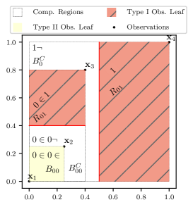
(a) An sMPT on ${\mathcal{D}}=\textsf{box}\left(\{{\mathbf{x}}_{1},\dots,{\mathbf{x}}_{4}\}\right)$. Strings in the top left of any box denote the encoding of that part of the space under the random partitioning; set notation corresponds to leaves of Fig. 2b

decision tree [$\epsilon:P_{\epsilon}=1.0$,plain content [$R_{0}$;μ_χ_ϵ,plain content,elo=yshift=4pt [$B_{0}$;μ_ρ_0,plain content [R_00;μ_χ_00 [B_00;μ_ρ_00] [B_00^C;1 - μ_ρ_00] ] [R_01;1 - μ_χ_00] ] [$B_{0}^{C}$;μ_1 - ρ_0,plain content] ] [$R_{1}$;1 - μ_χ_ϵ,plain content,elo=yshift=4pt ] ] ]

(b) The sMPT with parameters indicating mass distribution and space partition from Fig. 2a

Figure 2: A streaming Mondrian Pólya Tree. From left to right, the leaf/data encodings are: $\{(0\in 0\in:\{{\mathbf{x}}_{1},{\mathbf{x}}_{2}\}),\{(0\in 0\neg:\text{complementary leaf}),(0\in 1:\{{\mathbf{x}}_{3}\}),(1\neg:\text{complementary leaf}),(1:{\mathbf{x}}_{4})\}$

The standard Mondrian Tree only considers (sub-)regions where data is observed: information about space without observations is discarded. We decouple the splitting method used to generate Mondrian Trees into a two-step procedure which will allow a tree sampled in the Mondrian Tree $T\sim\textsf{MT}\left({\mathbf{X}},\lambda\right)$ to implicitly represent the entirety of a given input domain so we can appeal to the Pólya Tree model.

Our modified Mondrian Tree is the streaming Mondrian Pólya Tree (sMPT) and draws from this structure are denoted $T\sim\textsf{sMPT}\left({\mathbf{X}},\lambda\right)$. We generate an sMPT by drawing $T\sim\textsf{MT}\left({\mathbf{X}},\lambda\right)$ and introducing ‘pseudosplits’ in $T$ to generate a new, implicitly defined $T_{s}$. These pseudosplits distinguish between the regions of space where data is observed, and those which do not contain any data so the only extra space cost we incur is that of storing the parameters for the Beta distributions necessary for the Pólya Tree. An example is illustrated in Fig. 2a and is implemented in Alg. 3.

Let $T=(\mathsf{T},{\bm{\delta}},{\bm{\xi}},{\bm{\tau}})\sim\textsf{MT}\left({\mathbf{X}},\lambda\right)$ be a Mondrian Tree. We define two functions over nodes $j\in\mathsf{T}$ to decouple the cutting of space from the restriction to bounding boxes. First recall that every node $j$ has a minimal axis-aligned bounding box $B_{j}$: (i) $\texttt{cut}\left(j\right)$ samples a cut dimension $\delta_{j}$ and cut location $\xi_{j}$ splitting $j$ into disjoint sets $R_{j0},R_{j1}$ with $R_{j0}\cup R_{j1}=B_{j}$, and $R_{j0},R_{j1}$ representing the region of space less than cut $\xi_{j}$ and greater than $\xi_{j}$, respectively. For $k=0,1$, the set $R_{jk}$ is a bounded region of space which is not restricted to the observations located at the child nodes ${\mathbf{X}}_{N(\textsf{child}\left(j\right))}$. This motivates the subsequent ‘split’ to maintain the Mondrian Tree structure of only performing $\texttt{cut}\left(\cdot\right)$ on bounding boxes of observed data; (ii) $\texttt{restrict}\left(j\right)$ acts on the pair $R_{j0},R_{j1}$, returning $\left\{\left(B_{\textsf{left}\left(j\right)},B_{\textsf{left}\left(j\right)}^{C}\right),\left(B_{\textsf{right}\left(j\right)},B_{\textsf{right}\left(j\right)}^{C}\right)\right\}$ such that $B_{\textsf{left}\left(j\right)}\cup B_{\textsf{left}\left(j\right)}^{C}=R_{j0}$ and are pairwise disjoint. The same property holds for $R_{j1}$ with the right-hand child nodes. We refer to $B_{\textsf{child}\left(j\right)}$ as the observed region and $B_{\textsf{child}\left(j\right)}^{C}$ as the complementary region where $\textsf{child}\left(j\right)$ can be either $\textsf{left}\left(j\right)$ or $\textsf{right}\left(j\right)$. We term this as a ‘pseudosplit’ because all of the information required to perform $\texttt{restrict}\left(\texttt{cut}\left(j\right)\right)$ is already defined in the generation of the Mondrian Tree.

Combining sMPT with Finite Pólya Tree. Decoupling the ‘cut-then-restrict’ allows the Mondrian Tree $T$ to encode a valid hierarchical partition over the entirety of the input domain ${\mathcal{D}}$. Additionally, we only ever store the $T$ and the extra Beta parameters from the Pólya Tree structure as $T$ implicitly defines the sMPT $T_{s}$. These Beta parameters are cut parameters: $\chi_{j0},\chi_{j1}$, index 0 for less than $\xi_{j}$, 1 otherwise; restriction parameters $\rho_{j0\in},\rho_{j0\neg}$ indexed by $j0\in$ for the observed region $B_{\textsf{left}\left(j\right)}$ and $j0\neg$ for the complementary region $B_{\textsf{left}\left(j\right)}^{C}$ (and similarly for $\rho_{j1\in},\rho_{j1\neg}$) at node $j$.

The following distinctions are necessary to ensure all volume comparisons for the Pólya Tree construction are on $D$-dimensional hypervolumes while the final distinction is necessary to account for the mass associated to regions with no observations. (i) Observation leaves (Type I): Any leaf $l$ for which the bounding box at $l$, $B_{l}=\textsf{box}\left(X_{N(l)}\right)$ has at least one of the dimensions with zero length. Note that this includes the case when only one datapoint is stored in $l$; (ii) Observation leaves (Type II): Any leaf $l$ formed from a cut at node $j$ which contains two or more datapoints and $B_{l}=\textsf{box}\left(X_{N(l)}\right)$ has all $D$ lengths positive; (iii) Complementary leaves: Leaves formed in a region where no observations are made.

Pseudosplits in the Mondrian Tree $T$ are used to generate the sMPT, so it is necessary to revise the indexing scheme of the nested partition over domain ${\mathcal{D}}$. For every node $j\in\mathsf{T}$ of (absolute) depth $k$ in $T$, we generate a set of encodings for the spaces represented in $T_{s}$: $b(j)=c_{0}r_{0}\dots c_{k}r_{k}$. The length of $b(j)$ is at most twice the maximum absolute depth of $T$ and indexes all nodes in the (implicitly defined) $T_{s}$. The symbol $c_{i}\in\{0,1\}$ indicates “less than” or “greater than” the cut at level $i$, and $r_{i}\in\{\in,\neg,\emptyset\}$ indicates whether the node represents the observed region ($\in$), complementary region ($\neg$), or can be $\emptyset$ if the leaf is a Type I observed leaf as no restriction is performed.

3.1.1 Model Parameters for the sMPT

For a Mondrian Tree $T=(\mathsf{T},{\bm{\delta}},{\bm{\xi}},{\bm{\tau}})$ we now show how to set the parameters for the Pólya Tree over the induced sMPT, $T_{s}$.

• Let $P_{j}$ denote the probability mass associated with node $j$. We define the probability mass associated with the root $\epsilon$ to be $P_{\epsilon}=1$.

• Setting the prior. At every internal node $j\in\mathsf{T}$, the probability of a point being greater than the cut $\xi_{j}$ is given by a Bernoulli with parameter $\kappa_{j}$ whose prior is $\text{Beta}\left(\chi_{j0},\chi_{j1}\right)$. Likewise, the probability of a point being in the observed region after cut $\xi_{j}$ follows a $\text{Bernoulli}(1-\theta_{j})$ whose prior is $\text{Beta}\left(\rho_{jk\in},\rho_{jk\neg}\right)$ for $k=0,1$, depending on which side of the cut the point lies. To set the Pólya Tree parameters, we need to evaluate the volumes of various parts of the space, this will be denoted $V_{X}=\text{vol}\left(X\right)$ for $X\in\{R_{\cdot},B_{\cdot},B_{\cdot}^{C}\}$. The sMPT $T_{s}$ is defined from a two-stage split so we correct the ‘depth’ of nodes in $T_{s}$ from the usual Pólya Tree construction by a simple translation: if $j\in\mathsf{T}$ has depth $d_{j}$ then $\textsf{PolyaDepth}\left(j\right)=(2d_{j},2d_{j}+1)$. The prior strength is controlled by hyperparameter $\gamma>0$. Parameters for cut ($\chi_{\cdot}$) and restriction ($\rho_{\cdot}$) are then:

  $$\begin{split}\chi_{j0}&=\gamma(2d_{j}+1)^{2}\nicefrac{{V_{R_{j0}}}}{{(V_{R_{j0}}+V_{R_{j1}})}}\\ \chi_{j1}&=\gamma(2d_{j}+1)^{2}\nicefrac{{V_{R_{j1}}}}{{(V_{R_{j0}}+V_{R_{j1}})}}\\ \end{split}\quad\begin{split}\rho_{jk\in}&=\gamma(2d_{j}+2)^{2}\nicefrac{{V_{B_{jk\in}}}}{{(V_{B_{jk\in}}+V_{B_{jk\neg}})}}\\ \rho_{jk\neg}&=\gamma(2d_{j}+2)^{2}\nicefrac{{V_{B_{jk\neg}}}}{{(V_{B_{jk\in}}+V_{B_{jk\neg}})}}\\ \end{split}$$ (1)

• Distributing Mass. The predictive distribution of the Pólya Tree over a finite depth partition is the product of expected value of Beta distributions on the leaf-root path. There can be maintained exactly over all nodes for both cutting & restricting. We allocate a $\mu_{\chi_{j}}=\mathbb{E}(\text{Beta}\left(\chi_{j0},\chi_{j1}\right))$ fraction of $j$’s mass to $R_{j0}$ so $P_{j0}=P_{j}\mu_{\chi_{j}}$ & $P_{j1}=P_{j}(1-\mu_{\chi_{j}})$. Next, we repeat for the restriction step which allots $\mu_{\rho_{j0}}=\mathbb{E}(\text{Beta}\left(\rho_{j0\in},\rho_{j0\neg}\right))$ to $B_{j0}$ so $P_{j0\in}=P_{j0}\mu_{\rho_{j0}}$ and $P_{j0\neg}=P_{j0}(1-\mu_{\rho_{j0}})$; likewise for above the cut $\xi_{j}$.

• The Posterior Distribution. By Beta-Binomial conjugacy, on inserting data, the parameters of any given Beta distribution can be updated by the number of datapoints observed at a node. In the Mondrian Tree, $n_{0}$ points are passed from $j$ to $\textsf{left}\left(j\right)$ and $n_{1}$ points to $\textsf{right}\left(j\right)$. Hence, all of the $n_{0}$ points in $\textsf{left}\left(j\right)$ are both at most the cut value $\xi_{j}$ and present in the bounding box $B_{\textsf{left}\left(j\right)}$ while the opposite is true for $n_{1}$ and $\textsf{right}\left(j\right)$. Therefore, we obtain the simple posterior update procedure:

  $$\chi_{jk}^{*}=\chi_{jk}+n_{k},\quad\rho_{jk\in}^{*}=\rho_{jk\in}+n_{k},\quad\rho_{jk\neg}^{*}=\rho_{jk\neg},\quad\mbox{for }k=0,1$$ (2)

• Mass in the leaves of a finite Pólya Tree is assumed to be distributed uniformly; if a point falls into a leaf $j$, then the mass associated to that point is simply the product of the expected Beta distributions on the path from $\epsilon$ to $j$, and its density is the mass divided by the volume.

It is necessary to retain the volumes of both observed and complementary regions for the restriction parameters. However, this is straightforward given the cut and volume at node $j$ (see Appx. B).

Complexity: Instantiating the sMPT. The complexity of combining the Pólya Tree with the Mondrian Tree incurs only mild overhead. Let $T=(\mathsf{T},{\bm{\delta}},{\bm{\xi}},{\bm{\tau}})$ denote the stored Mondrian Tree which generates the sMPT. The extra space necessary to use sMPT for density estimation is $7|\mathsf{T}|$ due to the extra counters needed for every Beta distribution (i.e. $\chi_{j0},\chi_{j1},\rho_{jk\in},\rho_{jk\neg},k=0,1$) and the probability mass float $P_{j}$. At every node we must compute the volume at a cost of $O(D)$ which is $O(D|\mathsf{T}|)$ over the entire tree but this can be done on-the-fly as the tree is constructed.

sMPT: Insertions and Deletions. For a sMPT, we provide efficient algorithms to insert and delete points over the data stream. A full treatment is given in Appx. B: the pertinent points being that we retain projectivity due to the underlying Mondrian Tree which generates the sMPT. Deletions require a little more work as removal points could lie on a bounding box, so it is necessary to check how this interacts with the lifetime of the stored tree.

Example. In Fig. 2 we present an instantiation of the sMPT. Observe that the Mondrian Tree which is used to generate the partition in Fig. 2a splits the entire input domain into disjoint subsets of Type I/II observed leaves and complementary regions. It also implicitly encodes the associated sMPT as given in Fig. 2b. The calculations to obtain density estimates over this tree are given in Appx. C.

3.2 Mondrian Pólya Forest for Density Estimation & Anomaly Detection

Recall that an independently sampled ensemble of batch/streaming Mondrian Pólya Trees is referred to as a batch/streaming Mondrian Pólya Forest (bMPF), (sMPF), $F=\cup_{i}T_{i}$. Each $T_{i}$ defines a function over its leaves $p_{i}({\mathbf{x}})$ which is a noisy estimate of the true underlying density function $p({\mathbf{x}})$.

Definition 3.1 (Density Estimation).

Let $p({\mathbf{x}})$ be a density function and suppose $F=\cup_{i}T_{i}$ is a bMPF or sMPF. Let $l$ denote the leaf in $T_{i}$ which contains ${\mathbf{x}}$ and whose mass is $P^{(i)}_{l}$. The density estimate of ${\mathbf{x}}$ in $T_{i}$ is $p_{i}({\mathbf{x}})=P_{l}/\text{vol}\left(l\right)$ while the density estimate over the forest is $\hat{p}({\mathbf{x}})=\frac{1}{n}\sum_{i=1}^{|F|}p_{i}({\mathbf{x}})$.

Rather than using density estimates, we adopt the following simple approach to declare anomalies while remaining in probability space; using simply the $P^{(i)}_{l}$ rather than $p_{i}({\mathbf{x}})$. This alteration is to prevent a small number of trees from corrupting the ‘score’ if they are not good trees.

The simplicity of this approach is one of the strengths of our work. While previous works add an extra scoring mechanism over the forest, ours is an inherent property of the underlying probabilistic framework. We can threshold exactly in probability space which makes these ‘scores’ more interpretable than prior work. Synthetic density estimation & anomaly detection examples are in Appx. E.

Definition 3.2 (${\varepsilon}$-anomaly & $({\varepsilon},\phi)$-anomaly).

Let $F=\cup_{i}T_{i}$ be a bMPF or sMPF and ${\varepsilon},\phi\in[0,1]$. A point ${\mathbf{x}}\in\mathbb{R}^{d}$ is an ${\varepsilon}$-anomaly in tree $T$ if the probability mass of the leaf in which ${\mathbf{x}}$ is stored is at most ${\varepsilon}$. A point ${\mathbf{x}}\in\mathbb{R}^{d}$ is an $({\varepsilon},\phi)$-anomaly if ${\mathbf{x}}$ is and ${\varepsilon}$-anomaly in at least $\phi|F|$ trees from $F$.

4 Related Work

Initiated by the success of the so-called isolation forest (iForest) [20], random forest data summaries have become increasingly popular. The iForest algorithm can be roughly stated as: (i) sample a feature $u$ uniformly at random, (ii) Along $u$ sample a cut location $c$ uniformly at random & recurse either side of $c$ until the tree has reached maximum height. Anomalies are then declared based upon their average depth over the forest, under the expectation that points far from the expected behaviour are easier to identify so are ‘isolated’ more easily in the tree and have small average depth. Cuts exist on the entire (sub-)domain over which they are defined. That is, any cut is continued until it intersects another cut or a boundary, similar to the Mondrian Process.

However, it was noticed that uniformly sampling features in iForest could perform suboptimally: the RRCF rectifies this by sampling features to cut according to their length [17]. Cuts are restricted to the (sub-)regions of space where data is observed (just as in the Mondrian Tree) which enables efficient dynamic changes of the tree as data is added or removed. Given a tree $T$ sampled over data ${\mathbf{X}}$, these modifications ensure that the alteration of $T$ to $T^{\prime}$ by adding or removing ${\mathbf{u}}$ has the same distribution as sampling $T$ on ${\mathbf{X}}\cup\{{\mathbf{u}}\}$ or ${\mathbf{X}}\setminus{\mathbf{u}}$, respectively (Lemmas 4 and 6 of [17]). The scoring method is related to the expected change in depth of a node were a point (or group of points) not observed; the intuition being that anomalous points cause a significant change in structure when ignored.The RRCF also acts as a distance-preserving sketch in the $\ell_{1}$ norm, suggesting that this data structure is more general than its common use-case for anomaly detection. Interestingly, an extension of Mondrian Forests appears to exploit similar properties for estimating the Laplacian Kernel [6].

Finally, the Partial Identification Forest (PIDForest) is a $k$-ary tree for $k\geq 2$. In contrast to the previous two approaches, the splits are optimised deterministically over a uniform subsample of the input data to maximise the variance between sparsity across subgroups on a feature. The sparsity of a set of points is roughly the volume of the point set normalised by the volume of the region enclosed by a cut. It could be problematic to adapt the cuts for removed or new datapoints, so the PIDForest may not be ideal for heterogeneous data streams.

5 Anomaly Detection Experiments

Datasets. We test on all datasets from the open data repository in the Python Outlier Detection library (PyOD) ([31],[25]) & selected streaming datasets from the Numenta Anomaly Benchmark repository [2], [5]. The data are summarised in Tab. 3, Appx. D, ranging over $n\approx 10^{2}-O(10^{5})$ & $D\approx 10-400$. A mixture of batch & streaming data are present, as well as data containing continuous & categorical variables. The prevalence of anomalies ranges from $0.03\%$ to $36\%$. For stability in the volume computations MinMax feature scaling into $[0,1]$ was performed for $D\geq 50$. Univariate streaming datasets were transformed into 10 dimensions by applying the common ‘shingling’ technique of combining 10 consecutive points into one feature vector. As in [16], our performance metric is the area under curve (AUC) for the receiver operating charactersitic (ROC) curve.

Our Approach. We sample a forest $F=\cup_{i}T_{i}$ of 100 trees on the data ${\mathbf{X}}$ of batch or streaming Mondrian Pólya Trees (bMPF & sMPF). Both bMPF & MPF should have a lifetime parameter (weighted depth) to govern the length of the trees but competing methods are more traditional $k$-ary trees so we choose $\lambda=\infty$ (as in [19]) and set a max absolute depth of 10 for consistency with [16].

Competing Methods. We test against the following random forest algorithms for anomaly detection: Isolation Forest (iForest), Robust Random Cut Forest (RRCF) and PIDForest. For both RRCF & PIDForest we utilised opensource implementations available at [8] & [28]; all other methods are implemented in scikit-learn [23]. For the most meaningful comparison with [16], we adopt exactly their experimental methodology using default parameters for all scikit-learn methods, a forest of size 500 with at most 256 points for RRCF, and 50 trees of depth 10 over a uniform sample of 100 points for PIDForest. Results for non-random forest approaches (e.g. $k$NN,PCA) are in Tab. 5, Appx. D.

Performance Summary. The batch methods (bMPF, iForest, PIDForest) all generate static data structures. Although the internal parameters can be incremented on observing data, the structures do not easily adapt to streaming data. The two streaming methods (sMPF, RRCF) are adaptive structures which can be easily maintained on observing new data. We compare the batch methods and streaming methods separately: our results are summarised in Tab. 1 which shows that our batch and streaming solutions perform comparably to prior state of the art. The full AUC results over the entire PyOD repository are given in Tab. 4 which subsumes the previous benchmark in [16]. Note that we have not optimised parameter choices for performance, indicating that the parameter settings for bMPF, sMPF are good defaults - an important feature for anomaly detection. An advantage of both bMPF & sMPF is that they both use the same underlying data structures as iForest & RRCF while adding additional lightweight probabilistic structure relying only quantities that can be computed easily from the stored parameters at every node (e.g volumes).

Table 1: Mean Rank and Num. wins for all methods. The batch methods are tested separately from the streaming methods (sMPF, RRCF).

	bMPF	iForest	PidForest	sMPF	RRCF
Mean Rank	1.94	1.77	2.29	1.47	1.53
Num. Wins	18	24	16	32	28

Conclusion.

We have introduced the random forest consisting of Mondrian Pólya Trees. These trees have natural interpretations as density estimators of the underlying distribution of data. Our approach relates open questions concerning anomaly detection in [18] through the lens of density estimation, thus resolving the open question in [7]. Our method enables interpretable anomaly detection as we can threshold in the probability domain and use masses rather than densities.

In addition, our random forest can be maintained on a dynamic data stream with insertions and deletions, thus allowing the scalability required for large-data. In future work, we plan a more in-depth analysis of the performance on data streams and a rigorous study of the Mondrian Pólya Tree as a density estimator and change-point detector, rather than simply an anomaly detector.

Finally, there are several directions in which this work could be extended to allow scalability to higher dimensions by applying random rotations and/or projections after cuts. This has the effect of introducing oblique cuts into the space as opposed to axis-aligned cuts, and could be of further benefit. Another area for investigation would be to study the effect of approximate counting for the Pólya Tree parameters using sketches such as, for example, the CountMin sketch.

Broader Impact

Important applications of anomaly detection include cybersecurity intrusion detection, operational metrics monitoring, IoT signals (such as detecting broken sensors), and fraud detection. Thus, our contribution can have impact across all these domains. While there are many applications of varying ethical value that use anomaly detection, such as the possibility for misuse by a surveillance state to "detect anomalous citizen behavior", we believe that by focusing on the addition of interpretability to this solution helps to mitigate the misuses possible and allow better auditing of systems that do make use of anomaly detection [9].

One application in this domain where there are fairness concerns is regarding the rate of "anomalies" triggered by certain subgroups in fraud detection. A poorly calibrated or heuristic measure of anomalous behavior in this setting has the potential to discriminate against subgroups, where the data may be more sparse and thus more likely to appear anomalous. In this case, additional interpretability of how the model chooses anomalies is extremely important, as it allows the system operator to properly calibrate, using existing probabilistic fairness techniques, to remove or otherwise mitigate discrimination [13].

We present a method that enhances the state of the art for streaming anomaly detection by casting the problem as one of probabilistic density estimation. Modeling the problem in this way brings the immediate benefit of interpretability in the anomaly space: typical approaches such as thresholding at say 3 standard deviations away from the mean or median is a standard way of declaring outliers in applications but may not be suitable in settings when arbitrary scoring metrics are proposed Importantly however, the reframing of this into probability space allows future work to integrate other important socio-technical properties such as privacy and fairness into the same solution, for which there is much research in the field.

Developing accurate, efficient methods for dealing with or summarizing streaming data has the potential to reduce environmental impact significantly, as summarized data is less expensive to send and dealing with data in a localized manner (i.e. on device) removes the need to send data into the cloud for further computation. This enhancement of downstream analytics also inherently allows for more privacy, by aggregating less raw data together in the cloud. Additional research into how streaming summary methods can be applied in such cases is an exciting area in the preservation of user privacy. Privacy, differential privacy in particular, in the regime of anomaly detection involves a trade-off between knowing enough about a particular data point to determine its anomaly status and the plausible deniability of that data-point. Improving the capabilities of private, useful models for anomaly detection could be an important area for future work; for example, integrating existing differential privacy models for kd-trees [12] with the interpretable anomaly detectors we have proposed.

Appendix A Sampling Mondrian Trees, Pólya Trees and Mondrian Pólya Trees

Table 2: Lay summary of the various methods explored in our work.

Phrase	Lay Summary
Bayesian Nonparametrics
Mondrian Process	A binary tree which partitions sequentially partitions a space by cutting features. Cut dimensions chosen with probability proportional to length. Every node has a time. These trees are parametrised by the lifetime $\lambda>0$ but may be infinite if the sum of cutting times repeatedly lies slightly less than $\lambda$
Mondrian Tree	A binary tree which partitions an input space by cutting features. Cut dimensions are chosen with probability proportional to length. All nodes have times. Tree is guaranteed to be finite.
Pólya Tree	A probabilistic structure which takes as input any binary partition and distributes mass throughout the partition. Partition can be finite or infinite
Anomaly Detectors
iForest	Random forest generated by subsampling the dataset & building a binary tree. Feature $u$ sampled uniformly followed by a uniformly sampled cut in $u$. The scoring mechanism is average depth: anomalous points are easy to isolate so will have a low average depth compared to normal points.
RRCF	Random forest generated by subsampling the dataset & building a binary tree. Feature $u$ sampled with probability proportional to length. Cut location uniformly sampled cut in $u$. The scoring mechanism is “codisplacement”: the expected change in the structure of a tree were a group of points not observed.
PidForest	Random forest generated by subsampling the dataset & building a $k$-ary tree for some $k$ to be chosen. Features and cut locations chosen deterministically. The scoring mechanism is “sparsity”: roughly the volume of a pointset divided by the volume of the region enclosing it.

For clarity we describe the structures necessary to introduce our Mondrian Pólya Trees which are summarised in Tab. 2. We will begin with the Mondrian Process which can be succinctly described as: given an input domain ${\mathcal{D}}$ and a lifetime $\lambda>0$, choose a direction (feature) to cut with probability proportional to length. Next, choose a cut location uniformly at random on the selected feature and split into two sets less than and greater than the cut location. This cut procedure has a random cost associated to the “linear dimension” (sum of the lengths) of the region at a given node and the process is repeated until the lifetime is exhausted by accumulating the random costs. An implementation is given in [26].

The Mondrian Tree builds on the Mondrian Process by building the trees in a more data-aware fashion. At a high-level this process is similar to the Mondrian Process except every cut takes place on a restriction of space to the bounding box on which observations are made. The advantage of this is that cuts are guaranteed to pass through observations which in high dimensions could result in substantially shortened trees. Mondrian Trees can also be sampled online which makes them highly efficient. However, the price to pay for these efficiency gains is that behaviour outside of the bounding boxes cannot be modelled.

While the previous two methods are useful for partitioning the data into clusters, they make no statements about the underlying density of the dataset. To accommodate this we introduce the Pólya Tree which is a Bayesian nonparametric model for estimating the underlying density function generating the data. The Pólya Tree model takes as input a binary nested partition of an input space ${\mathcal{D}}$, (represented by a binary tree) and assigns probability to each of the bins (nodes in the tree). Given a point in a bin indexed $A_{b(j)}$, the presence of a point in the bins $A_{b(j)1}$ is modelled by a Bernoulli distribution with parameter $p$. Let $d_{j}$ denote the depth of $A_{b(j)}$ and $V_{0},V_{1}$ denote the volumes of the the bins $A_{b(j)0},A_{b(j)1}$, respectively. The prior distribution for $p$ is a Beta distribution which has parameters:

$$\alpha_{j0} =\gamma\left(d_{j}+1\right)^{2}\frac{V_{0}}{V_{0}+V_{1}}$$ (3)

$$\alpha_{j1} =\gamma\left(d_{j}+1\right)^{2}\frac{V_{1}}{V_{0}+V_{1}}$$ (4)

for a hyperparameter $\gamma>0$ denoting the strength of the prior distribution. The posterior parameters for the $\alpha_{jk}$ are then incremented by the number of points observed in the $A_{b(j)k}$ bin for $k=0,1$. An implementation is given in Alg. 2 which takes as input the partition of space ${\mathcal{D}}$, thus requiring an extra pass through the tree. However, for our applications as defined in Sec. 3.2, we will be able to implement this in an online fashion.

Our Mondrian Pólya Tree can be implemented in either a batch or streaming fashion. For a batch computation, we can adapt the Mondrian Process and easily combine this with the Pólya Tree. However, for streaming computation, the ‘empty space’ caused by restricting to bounding boxes in the Mondrian Tree procedure is highly problematic and this motivated our revised construction, the sMPT as described in Sec. 3.1. We describe this revision in Alg. 3 while the parameter update algorithms are presented in Alg. 4.

Generating Mondrian Pólya Trees: Computational Complexity. Combining the Pólya Tree with either the Mondrian Process or Mondrian Tree incurs only a mild overhead in both time and space as all that needs to be stored is an extra set of parameters. For the batch Mondrian Pólya Tree (Sec. 3) this is simply 3 counters per node ($\alpha_{j0},\alpha_{j1},P_{j}$). In Sec. 3.1 we showed that a two-stage split was necessary for the streaming Mondrian Pólya Tree and this slightly increases the number of parameters to at most 7 per node (see 3.1.1) which come from the 2 cut parameters, at most 4 restriction parameters, and the mass float $P_{j}$. Overall, both methods need $O(|\mathsf{T}|)$ extra space which, nevertheless, is only a constant factor more space than is required to build the partitioning tree.

The time cost to evaluate these parameters is $O(d|\mathsf{T}|)$ as computing the volume of every node costs $O(d)$. Since we make the distinction between type I/II observation & complementary leaves, volume comparisons are made over nonzero $D$-dimensional hypervolumes. This permits the following distinctions at every node to avoid incurring complex volume computations of the complementary regions.

Volume Computation for sMPT. Recall that for a node $j$ we sample a cut dimension $\delta_{j}$ and in that dimension a cut location $\xi_{j}$. The node $j$ contains the restriction to bounding box $B_{j}$ which is split into two regions $R_{j0}$ and $R_{j1}$ either side of $\xi_{j}$. Node $j$ has volume $V_{B_{j}}=\text{vol}\left(j\right)$ and let $h_{j}$ denote the length of the sampled dimension $\delta_{j}$; the volumes associated with $R_{j0}$ and $R_{j1}$ are:

$$V_{R_{j0}} =\frac{V_{B_{j}}}{h_{j}}|\min_{{\mathbf{x}}\in j}{\mathbf{x}}_{\delta_{j}}-\xi_{j}|$$ (5)

$$V_{R_{j1}} =\frac{V_{B_{j}}}{h_{j}}|\max_{{\mathbf{x}}\in j}{\mathbf{x}}_{\delta_{j}}-\xi_{j}|.$$ (6)

We obtain the volume of the observed region when computing $\texttt{restrict}\left(j\right)$ for the restriction to bounding boxes either side of the cut $\xi_{j}$ at $j$. Recall that $V_{\textsf{left}\left(j\right)}=\text{vol}\left(B_{\textsf{left}\left(j\right)}\right)$, so the subtraction $V_{R_{j0}}-V_{\textsf{left}\left(j\right)}=V_{B_{j0}^{C}}$ yields the complementary volume necessary for setting the restriction Pólya parameters $\rho_{\cdot\in},\rho_{\cdot\neg}$. All volumes being supported on $D$-dimensional boxes ensures that none of these quantities trivially collapse to zero. If one of the feature lengths is zero then we simply treat such a node as a Type I observation leaf.

Input: Training data ${\mathbf{X}}\in\mathbb{R}^{n\times D}$, lifetime $\lambda>0$

1 Function SampleMondrianTree(${\mathbf{X}},\lambda$):

2       Initialise $\mathsf{T}=\emptyset,\textsf{leaves}\left(\mathsf{T}\right)=\emptyset,{\bm{\delta}}=\emptyset,{\bm{\xi}}=\emptyset,{\bm{\tau}}=\emptyset,N(\epsilon)=\{1,2,\dots,n\}.$

3       SampleMondrianBlock($\epsilon,{\mathbf{X}}_{N(\epsilon)},\lambda$)

4      

5 Function SampleMondrianBlock($j,{\mathbf{X}}_{N(j)},\lambda$):

6       $\mathsf{T}\leftarrow\mathsf{T}\cup\{j\}$

7       For all $d\in[D]$ set ${\mathbf{l}}_{jd}^{{\mathbf{X}}}=\min_{d}{\mathbf{X}}_{N(j)},{\mathbf{u}}_{jd}^{{\mathbf{X}}}=\max_{d}{\mathbf{X}}_{N(j)}$ to be the dimension-wise minima and maxima of the observations in $j$

8       Let $L=\sum_{d}(u_{jd}^{{\mathbf{X}}}-l_{jd}^{{\mathbf{X}}})$ denote the linear dimension of the data in $j$

9       Sample $E\sim\text{Exp}\left(L\right)$

10       if $\tau_{\textsf{parent}\left(j\right)}+E<\lambda$ then

11             Set $\tau_{j}=\tau_{\textsf{parent}\left(j\right)}+E$

12             Sample cut dimension $\delta_{j}$ with probability proportional to $u_{jd}^{{\mathbf{X}}}-l_{jd}^{{\mathbf{X}}}$

13             Sample cut location uniformly on the interval $[l_{j\delta_{j}}^{{\mathbf{X}}},u_{j\delta_{j}}^{{\mathbf{X}}}]$

14            

15            Set $N(\textsf{left}\left(j\right))=\{n\in N(j):X_{n\delta_{j}}\leq\xi_{j}\}$ and $N(\textsf{right}\left(j\right))=\{n\in N(j):X_{n\delta_{j}}>\xi_{j}\}$

16            

17            SampleMondrianBlock($\textsf{left}\left(j\right),{\mathbf{X}}_{N(\textsf{left}\left(j\right))},\lambda$)

18             SampleMondrianBlock($\textsf{right}\left(j\right),{\mathbf{X}}_{N(\textsf{right}\left(j\right))},\lambda$)

19       else

20             $\tau_{j}\leftarrow\lambda$ and $\textsf{leaves}\left(\mathsf{T}\right)\leftarrow\textsf{leaves}\left(\mathsf{T}\right)\cup\{j\}$

21      

Algorithm 1 Mondrian Forest Sampling [19]

Input: Input domain ${\mathcal{D}}\subset\mathbb{R}^{D}$, a decision tree $T$ which partitions ${\mathcal{D}}$, hyperparameter $\gamma>0$

Output: Probability distribution ${\mathcal{P}}=(P_{l})_{l\in\textsf{leaves}\left(T\right)}$

1 Function SamplePólyaTree(${\mathcal{D}},T,\gamma$):

2       $\epsilon=\text{root}\left(T\right)$

3       $P_{\epsilon}=1$ $\triangleright$ Assume all mass is located in the region ${\mathcal{D}}$

4       UpdatePólyaParameters($\epsilon,\gamma$)

5      

6

7 Function UpdatePólyaParameters($j,\gamma$):

8       if $j\in\textsf{leaves}\left(T\right)$ then

9             $\text{ProbDensity}(j)=P_{j}/\text{vol}\left(j\right)$ $\triangleright$ $P_{j}$ was defined at the preceeding level.

10       else

11             $V_{j}=\text{vol}\left(j\right)$

12             Let $R_{j}=[l_{1},u_{1}]\times\dots\times[l_{d},u_{d}]$ define the region in as a product of intervals from the minimum in dimension $i$, $l_{i}$, to the maximum in dimension $i$, $u_{i}$.

13             $L_{j}=\sum_{j=1}^{d}(u_{j}-l_{j})$ is the linear dimension of the region.

14             $V_{0}=\frac{V_{j}}{u_{\delta_{j}}-l_{\delta_{j}}}\cdot|l_{\delta_{j}}-\xi_{j}|$ $\triangleright$ Volume less than cut $\xi_{j}$

15             $V_{1}=\frac{V_{j}}{u_{\delta_{j}}-l_{\delta_{j}}}\cdot|u_{\delta_{j}}-\xi_{j}|$ $\triangleright$ Volume greater than cut $\xi_{j}$

16             $n_{0}=\text{NumberOfPoints}(\textsf{left}\left(j\right)),n_{1}=\text{NumberOfPoints}(\textsf{right}\left(j\right))$ $\triangleright$ Number of points in children nodes

17             $\alpha_{0}=\gamma(d+1)^{2}\frac{V_{0}}{V_{0}+V_{1}}+n_{0},\alpha_{1}=\gamma(d+1)^{2}\frac{V_{1}}{V_{0}+V_{1}}+n_{1}$ $\triangleright$ Set prior parameters using Pólya Tree  and then increment using Beta-Binomial conjugacy

18             $\mu_{j}=\frac{\alpha_{0}}{\alpha_{0}+\alpha_{1}}$ $\triangleright$ $\mathbb{E}(\text{Beta}\left(\alpha_{0},\alpha_{1}\right))$

19             $P_{\textsf{left}\left(j\right)}=\mu_{j}P_{j},P_{\textsf{right}\left(j\right)}=(1-\mu_{j})P_{j}$

20             UpdatePólyaParameters($\textsf{left}\left(j\right),\gamma$), UpdatePólyaParameters($\textsf{right}\left(j\right),\gamma$)

21      

Algorithm 2 Pólya Tree Sampling. Sets probability (density) for all nodes in the given random partition $T$.

Input: Training data ${\mathbf{X}}\in\mathbb{R}^{n\times D}$, at least one of lifetime $\lambda>0$ or maximum tree height $m$, Pólya Tree hyperparameter $\gamma>0$

Output: A classical Mondrian Tree data structure $T$; Partition $\Pi$ over $T$ such that ${\mathcal{P}}=(P_{l})_{l\in\textsf{leaves}\left(T\right)}$ is a probability distribution over the leaves of $T$ induced by Pólya Tree prior

1 Function SampleMondrianPólyaTree(${\mathbf{X}},\lambda$):

2       Initialise $\mathsf{T}=\emptyset,\textsf{leaves}\left(\mathsf{T}\right)=\emptyset,{\bm{\delta}}=\emptyset,{\bm{\xi}}=\emptyset,{\bm{\tau}}=\emptyset,N(\epsilon)=\{1,2,\dots,n\}.$

3       $\epsilon.\text{ObservedVolume}=\text{vol}\left(\textsf{box}\left({\mathbf{X}}_{N(\epsilon)}\right)\right)$

4       SampleMondrianPólyaBlock($\epsilon,{\mathbf{X}}_{N(\epsilon)},\lambda$)

5      

6 Function SampleMondrianPólyaBlock($j,{\mathbf{X}}_{N(j)},\lambda$):

7       $\mathsf{T}\leftarrow\mathsf{T}\cup\{j\}$

8       $B_{j}\leftarrow\textsf{box}\left({\mathbf{X}}_{N(j)}\right),L=\textsf{LinearDim}\left(B_{j}\right)$ $\triangleright$ linear dimension of the bounding box for $j$

9       Sample $E\sim\text{Exp}\left(L\right)$

10       if $\tau_{\textsf{parent}\left(j\right)}+E<\lambda\text{~{}and all feature lengths are positive}$ then

11             Set $\tau_{j}=\tau_{\textsf{parent}\left(j\right)}+E$

12             Cut($j,{\mathbf{X}}_{N(j)},B_{j}$)

13            

14            Set $N(\textsf{left}\left(j\right))=\{n\in N(j):{\mathbf{X}}_{n\delta_{j}}\leq\xi_{j}\}$ and $N(\textsf{right}\left(j\right))=\{n\in N(j):{\mathbf{X}}_{n\delta_{j}}>\xi_{j}\}$

15            

16            Restrict($j,N(\textsf{left}\left(j\right))$)

17             Restrict($j,N(\textsf{right}\left(j\right))$)

18            SampleMondrianPólyaBlock($\textsf{left}\left(j\right),{\mathbf{X}}_{N(\textsf{left}\left(j\right))},\lambda$)

19             SampleMondrianPólyaBlock($\textsf{right}\left(j\right),{\mathbf{X}}_{N(\textsf{right}\left(j\right))},\lambda$)

20       else

21             if any feature length is 0 then

22                   $\mathsf{T}\leftarrow\mathsf{T}\cup\{j\}$ $\triangleright$ Bounding box supported on $<d$ dimensions: Type I Observed leaf

23             else

24                   Restrict($j,N(j)$) $\triangleright$ Restrict once more to generate a complementary leaf

25                  

26            $\tau_{j}\leftarrow\lambda$ and $\textsf{leaves}\left(\mathsf{T}\right)\leftarrow\textsf{leaves}\left(\mathsf{T}\right)\cup\{j\}$ $\triangleright$ Type II Observed leaf (see Sec. 3.1)

27      

28

29 Function Cut($j,{\mathbf{X}}_{N(j)},B_{j}$):

30       Sample cut dimension $\delta_{j}$ with probability proportional to $u_{jd}^{{\mathbf{X}}}-l_{jd}^{{\mathbf{X}}}$

31       Sample cut location $\xi_{j}$ uniformly on the interval $[l_{j\delta_{j}}^{{\mathbf{X}}},u_{j\delta_{j}}^{{\mathbf{X}}}]$

32       ${R_{\textsf{left}}}=\{{\mathbf{z}}\in B_{j}:{\mathbf{z}}_{\delta_{j}}\leq\xi_{j}\}$

33       ${R_{\textsf{right}}}=\{{\mathbf{z}}\in B_{j}:{\mathbf{z}}_{\delta_{j}}>\xi_{j}\}$

34       $n_{\textsf{left}}=|{\mathbf{X}}_{N(j)}\cap{R_{\textsf{left}}}|$

35       $n_{\textsf{right}}=|{\mathbf{X}}_{N(j)}\cap{R_{\textsf{right}}}|$

36       $V_{\textsf{left}}=\text{vol}\left({R_{\textsf{left}}}\right),V_{\textsf{right}}=\text{vol}\left({R_{\textsf{right}}}\right)$

37       $d_{j}=\textsf{depth}\left(j\right)$ $\triangleright$ Absolute depth in Mondrian Tree

38       SetCutParameters($2d_{j},n_{\textsf{left}},n_{\textsf{right}},V_{\textsf{left}},V_{\textsf{right}}$)

39

40 Function Restrict($j,{\mathbf{X}}_{N(j)}$):

41       $d=j.\text{depth}$ $\triangleright$ Get absolute depth in Mondrian tree

42       $n_{\textsf{obs}}=|N(j)|$ $\triangleright$ Num. points in node

43       $V_{p}=\textsf{parent}\left(j\right).\text{ObservedVolume}$ $\triangleright$ Parent volume

44       $V_{o}=\text{vol}\left(B({\mathbf{X}}_{N(j)})\right)$ $\triangleright$ Observed volume

45       $V_{c}=V_{p}-V_{o}$ $\triangleright$ Complementary volume

46       $\rho_{0}^{*},\rho_{1}^{*}$ = SetRestrictionParameters($2d+1,n_{\textsf{obs}},V_{o},V_{c}$) $\triangleright$ Set Beta parameters.

47       return $\rho_{0}^{*},\rho_{1}^{*}$

48

Algorithm 3 Mondrian Pólya Tree Sampling. Subroutines: Alg. 4

1 Function SetCutParameters($\text{depth},n_{\textsf{left}},n_{\textsf{right}},V_{\textsf{left}},V_{\textsf{right}}$):

2       $d=\text{depth}$

3       $j.\chi_{0}^{*}=\gamma(d+1)^{2}\frac{V_{\textsf{left}}}{V_{\textsf{left}}+V_{\textsf{right}}}+n_{\textsf{left}},j.\chi_{1}^{*}=\gamma(d+1)^{2}\frac{V_{\textsf{right}}}{V_{\textsf{left}}+V_{\textsf{right}}}+n_{\textsf{right}}$

4      

5 Function SetRestrictionParameters($\text{depth},\text{NodeSize},\text{ObservedVolume},\text{ComplemetaryVolume}$):

6       $d=\text{depth};\qquad$ $n=\text{NodeSize}$ $\triangleright$ Number of points in observed bounding box

7       $V_{obs}=\text{ObservedVolume},V_{comp}=\text{ComplemetaryVolume}$

8       $\rho_{0}^{*}=\gamma(d+1)^{2}\frac{V_{obs}}{V_{obs}+V_{comp}}+n$, $\rho_{1}^{*}=\gamma(d+1)^{2}\frac{V_{comp}}{V_{obs}+V_{comp}}$

9       return $\rho_{0}^{*},\rho_{1}^{*}$

Algorithm 4 Subroutines for setting Beta Distribution parameters for the Mondrian Pólya Tree. Note that the depth parameters in these subroutines refer to depth in Pólya Tree, not absolute depth in Mondrian Tree!

Appendix B sMPT: Insertions and Deletions

A substantial benefit of the Mondrian Tree construction is that it can be built online as new data is seen. The key idea underpinning this is projectivity (Lemma 2.1 Sec. 2), which asserts that if a Mondrian tree $T\sim\textsf{MT}\left({\mathbf{X}},\lambda\right)$ is sampled and a new point ${\mathbf{z}}$ is observed, then inserting ${\mathbf{z}}$ into $T$ to generate $T^{\prime}$ yields $T^{\prime}\sim\textsf{MT}\left({\mathbf{X}}\cup{\mathbf{z}},\lambda\right)$ [19]; moreover, this process is efficient. This is where the restriction of a cut $\xi_{j}$ to the bounding box $B_{j}$ is critical, because it permits the sequential addition of ${\mathbf{z}}$ into $T$ while preserving the distribution over which $T$ was sampled had ${\mathbf{z}}$ been seen prior to sampling $T$! We adapt the online update procedures from Mondrian Trees to streaming Mondrian Pólya Trees by invoking projectivity and then recognising that the necessary parameters can be easily incremented as the data is observed. Inserting a point ${\mathbf{z}}$ into tree $T$ is denoted $T^{\prime}\sim\textsf{sMPT}_{+}\left(T,{\mathbf{z}}\right)$.

However, for data streams we also need the capability to delete from the tree; this is where the link with the RRCF work becomes necessary, as we can adapt their deletion mechanism for the Mondrian Pólya Tree setting. Our alteration is necessary for the Mondrian Tree setting as nodes have an associated time which cannot exceed the lifetime budget $\lambda$ and deleting a point on the bounding box can affect the times of all nodes in the subtree rooted at that node. In this setting, the point to delete, ${\mathbf{z}}$, is chosen ahead of time, hence the algorithm is deterministic which is why we will write $T^{\prime}=\textsf{sMPT}_{-}\left(T,{\mathbf{z}}\right)$ (in contrast to $T^{\prime}\sim\textsf{sMPT}_{+}\left(T,{\mathbf{z}}\right)$) for deleting ${\mathbf{z}}$ from $T$. The following lemmas summarise the insertion and deletion procedures from [19] and [17] to account for the additional Pólya Tree parameters that we need when using the Mondrian Pólya Tree. The insertions procedure is described in Alg. 5, and Alg. 6 illustrates the deletion mechanism.

Lemma B.1 (Insertions).

Let $T\sim\textsf{sMPT}\left({\mathbf{X}},\lambda\right)$ be a Mondrian Pólya Treesampled over data ${\mathbf{X}}$ with lifetime $\lambda>0$. If ${\mathbf{z}}$ is a new observation and $T^{\prime}\sim\textsf{sMPT}_{+}\left(T,{\mathbf{z}}\right)$ then $T^{\prime}\sim\textsf{sMPT}\left({\mathbf{X}}\cup{\mathbf{z}},\lambda\right)$.

Proof.

The tree that we sample and store is exactly a Mondrian Tree, hence we invoke projectivity so that $T^{\prime}$ is a valid Mondrian Tree over ${\mathbf{X}}\cup{\mathbf{z}}$. Since the Mondrian Tree $T$ implicitly but uniquely defines a Mondrian Pólya Tree which partitions the input space, projectivity also applies to the Mondrian Pólya Tree structure as a random partition. Additionally, we need to alter the (cut and restrict) Beta parameters for every node which are affected by the insertion of ${\mathbf{z}}$ in tree $T$. However, this amounts to simply incrementing counts over the subtree: updating the parameters is sufficient as we only need the expected value of every Beta distribution.

∎

Lemma B.2 (Deletions).

Let $T\sim\textsf{sMPT}\left({\mathbf{X}},\lambda\right)$ and let ${\mathbf{z}}$ be the point to be removed from ${\mathbf{X}}$ and $T$. If $T^{\prime}=\textsf{sMPT}_{-}\left(T,{\mathbf{z}}\right)$ then $T^{\prime}\sim\textsf{sMPT}\left({\mathbf{X}}\setminus{\mathbf{z}},\lambda\right)$.

Proof.

First, locate the deepest node $j$ containing ${\mathbf{z}}$, there are two cases: (i) ${\mathbf{z}}$ is internal to the box $B_{j}$ (ii) ${\mathbf{z}}$ is a boundary point defining part of the bounding box $B_{j}$ (i.e. it is maximal or minimal at $j$ in one dimension). If ${\mathbf{z}}$ is internal to $B_{j}$ then we are free to simply remove it from $j$ and decrement the necessary counts. Otherwise, deleting ${\mathbf{z}}$ causes a change to the bounding box: let $B_{j}^{\prime}$ denote the new bounding box for $j$ under the removal of ${\mathbf{z}}$. Now, it must be the case that $L_{j}^{\prime}=\textsf{LinearDim}\left(B_{j}^{\prime}\right)$ is at most $L_{j}=\textsf{LinearDim}\left(B_{j}\right)$. However, if there is a ${\mathbf{u}}\neq{\mathbf{z}}$ in $j$ but is equal to ${\mathbf{z}}$ in all dimensions on which ${\mathbf{z}}$ lies on the boundary, then we could treat ${\mathbf{z}}$ as an internal point and remove then decrement. So assume ${\mathbf{z}}$ uniquely defines $B_{j}$ in the required dimensions, hence $L_{j}^{\prime}<L_{j}$ so the exponential distribution used to generate the node time $\tau_{j}$ is different under the absence of ${\mathbf{z}}$. Let $F(t)=\textsf{CDF}\left(\text{Exp}\left(L_{j}\right)\right)(t)$ and $G(t)=\textsf{CDF}\left(\text{Exp}\left(L_{j}^{\prime}\right)\right)(t)$ be the CDF functions of the exponential distributions $\text{Exp}\left(L_{j}\right)$ and $\text{Exp}\left(L_{j}^{\prime}\right)$, respectively as functions of time $t$. The mass associated to time $\tau_{j}$ is $\psi=F(\tau_{j})$ hence, the time with the same mass in $G(t)$ is $\tau_{j}^{\prime}=G^{-1}(\psi)$ (these are straightforward for the exponential distribution since $\textsf{CDF}\left(\text{Exp}\left(\zeta\right)\right)(t)=1-\exp(-\zeta t)$). Finally, since $L^{\prime}<L$, we must have $\tau_{j}^{\prime}>\tau_{j}$ so the time has increased, meaning we must check whether $\tau_{j}^{\prime}<\lambda$. If so, then keep $j$, else contract $j$ and its descendants into $\textsf{parent}\left(j\right)$. This approach must be done for every node on the path from $\epsilon$ to $j$ which contains ${\mathbf{z}}$ so in the worst case is $O(d\cdot\textsf{depth}\left(T\right))$. Finally, it remains to decrement all necessary counts which were affected by the presence of ${\mathbf{z}}$ on the path from $\epsilon$ to $j$ (or the contracted ancestor of $j$). ∎

Complexity: Insertions & Deletions Both procedures are efficient and are dominated by the time it takes to locate the locate the node which stores query point and requires checking inclusion in a bounding box at $O(D)$ cost a maximum of $\textsf{depth}\left(T\right)$ times, hence $O(D\textsf{depth}\left(T\right))$ overall. Note that this is the absolute depth measured in the Mondrian Tree sense, not the adjusted depth to account for the Pólya Tree construction as defined prior to Eq. 1, nor the lifetime $\lambda$ which could potentially be large. Since we only store the Mondrian Tree which generates the Mondrian Pólya Tree which, in expectation, should be balanced and hence $\textsf{depth}\left(T\right)=\Theta(\log n)$. In the random forest literature ([20], [17], [16]), the depth is typically a parameter of small magnitude relative to the size of input data, usually 10. Hence, the presence of the maximum tree depth term in the above time complexity bounds is not problematic.

Input: Mondrian Tree $T=(\mathsf{T},{\bm{\delta}},{\bm{\xi}},{\bm{\tau}})$

Output: Mondrian Tree $T$ sampled over ${\mathbf{X}}\cup{\mathbf{z}}$

1 Function $\textsf{MT}_{+}$($T,{\mathbf{X}},\lambda,{\mathbf{z}}$):

2       $\epsilon=\textsf{root}(T)$

3       MTx($T,{\mathbf{X}},\lambda,{\mathbf{z}},\epsilon$)

4      

5 Function MTx($T,{\mathbf{X}},\lambda,{\mathbf{z}},j$):

6       ${\mathbf{e}}^{l}=\max(l_{j}^{{\mathbf{X}}}-{\mathbf{z}},0),{\mathbf{e}}^{u}=\max({\mathbf{z}}-u_{j}^{{\mathbf{X}}},0)$ $\triangleright$ ${\mathbf{e}}^{l},{\mathbf{e}}^{u}={\mathbf{0}}_{d}$ iff $z\in B_{j}$

7       Increment the observed restriction parameter $\rho_{0}$ by 1

8       Sample $E\sim\text{Exp}\left(\sum_{i=1}^{d}\left({\mathbf{e}}^{u}+{\mathbf{e}}^{l}\right)_{i}\right)$

9       if $\tau_{\textsf{parent}\left(j\right)}+E<\tau_{j}$ then

10             Sample $\delta$ with probability proportional to ${\mathbf{e}}^{u}+{\mathbf{e}}^{l}$

11             Sample a cut $\chi\sim\textsf{Uniform}\left(a,b\right)$ with $a=u_{j\delta}^{{\mathbf{X}}},b={\mathbf{z}}_{\delta}$ if ${\mathbf{z}}_{\delta}>u_{j\delta}$, else $a={\mathbf{z}}_{\delta},b=l_{j\delta}^{{\mathbf{X}}}$

12             Insert $j^{\prime}$ ($j$ but below $\textsf{parent}\left(j\right)$) to $j$ with: $N(j^{\prime})=N(j)\cup\{{\mathbf{z}}\}$, $\delta_{j^{\prime}}=\delta,\xi_{j^{\prime}}=\chi,\tau_{j^{\prime}}=\tau_{\textsf{parent}\left(j\right)}+E,l_{j^{\prime}}^{{\mathbf{X}}}=\min(l_{j}^{{\mathbf{X}}},{\mathbf{z}}),u_{j^{\prime}}^{{\mathbf{X}}}=\max(u_{j}^{{\mathbf{X}}},{\mathbf{z}})$

13             Insert sibling $j_{\textsf{sib}}$ containing ${\mathbf{z}}$ such that $\textsf{left}\left(j^{\prime}\right)=j,\textsf{right}\left(j^{\prime}\right)=j_{\textsf{sib}}$ if ${\mathbf{z}}_{\delta_{j}}>\xi_{j}$ or $\textsf{right}\left(j^{\prime}\right)=j,\textsf{left}\left(j^{\prime}\right)=j_{\textsf{sib}}$, otherwise

14             Set the Beta parameters according to number of points either side of $\xi_{j}$

15       else

16             Update $l_{j}^{{\mathbf{X}}}\leftarrow\min(l_{j}^{{\mathbf{X}}},{\mathbf{z}}),u_{j^{\prime}}^{{\mathbf{X}}}\leftarrow\max(u_{j}^{{\mathbf{X}}},{\mathbf{z}})$

17             if $j\in\textsf{leaves}\left(\mathsf{T}\right)$ then

18                   return

19             else

20                   if ${\mathbf{z}}_{\delta_{j}}<\xi_{j}$ then

21                         $\textsf{child}\left(j\right)=\textsf{left}\left(j\right)$

22                   else

23                         $\textsf{child}\left(j\right)=\textsf{right}\left(j\right)$

24                   Increment $\chi_{\textsf{child}\left(j\right)}$ by 1

25                   MTx($T,{\mathbf{X}},\lambda,{\mathbf{z}},\textsf{child}\left(j\right)$)

26            

27      

Algorithm 5 Mondrian Pólya Tree Insertion: $\textsf{sMPT}_{+}\left(T,{\mathbf{z}}\right)$

Input: Mondrian Tree $T=(\mathsf{T},{\bm{\delta}},{\bm{\xi}},{\bm{\tau}})$

Output: Mondrian Tree $T$ sampled over ${\mathbf{X}}\setminus{\mathbf{z}}$

1 Function $\textsf{MT}_{-}$($T,{\mathbf{X}},\lambda,{\mathbf{z}}$):

2       $\epsilon=\textsf{root}(T),\textsf{path}=\{\epsilon\}$

3       MTd($T,{\mathbf{X}},\lambda,{\mathbf{z}},\epsilon$)

4      

5 Function MTd($T,{\mathbf{X}},\lambda,{\mathbf{z}},j,\textsf{path}$):

6       Find the deepest node $j$ containing ${\mathbf{z}}$

7       Let $\textsf{path}=\{\epsilon,u_{1},u_{2},\dots,u_{k}\}$ be the set of nodes from $\epsilon$ to $j$

8       for $j\in\textsf{path}$ do

9             Check if ${\mathbf{z}}$ is internal to the bounding box, or a point which defines the bounding box in one of dimensions $i\in\{1,2,\dots,d\}$

10             if ${\mathbf{z}}$ is internal then

11                   $\textsf{child}\left(j\right)=\textsf{left}\left(j\right)$ iff ${\mathbf{z}}_{\delta_{j}}\leq\xi_{j}$ Decrement the cut and restriction counter corresponding to ${\mathbf{z}}$ at $v$ by 1

12                   Decrement all counts by 1 at the subtree rooted at $\textsf{child}\left(j\right)$ $\triangleright$ This only decrements on the side of the cut that ${\mathbf{z}}$ should go.

13                   return

14             else

15                   Let $B_{j}^{\prime}$ be the bounding box at $j$ with ${\mathbf{z}}$ ignored which has linear dimension $L^{\prime}=\textsf{LinearDim}\left(B_{j}^{\prime}\right)$

16                   Evaluate new node time $\tau_{j}^{\prime}$ through inverse CDF

17                   if $\tau_{j}^{\prime}\geq\lambda$ then

18                         Contract the entire subtree rooted at $j$ into $j$

19                         Set $\tau_{j}^{\prime}=\lambda$

20                         return

21                  

22            

23      return $T$

Algorithm 6 Inplace deletions for the Mondrian Pólya Tree, $\textsf{sMPT}_{-}\left(T,{\mathbf{z}}\right)$.

Appendix C Calculations for Fig. 2

Let us consider the generative process for sampling a streaming Mondrian Pólya Tree (sMPT) to clarify the interplay between the underlying Mondrian and Pólya Trees. Let ${\mathbf{X}}=\{{\mathbf{x}}_{1},{\mathbf{x}}_{2},{\mathbf{x}}_{3},{\mathbf{x}}_{4}\}$ with ${\mathbf{x}}_{1}=(0,0),{\mathbf{x}}_{2}=(1/4,1/4),{\mathbf{x}}_{3}=(2/5,4/5),{\mathbf{x}}_{4}=(1,1)$. Set ${\mathcal{D}}=\textsf{box}\left({\mathbf{X}}\right)$ to be the bounding box of the region containing ${\mathbf{X}}$ and denote the two directions which span $\mathbb{R}^{2}$ be $x$ and $y$. We show how sampling a depth 2 Mondrian Tree encodes a depth 4 sMPT which can be used to estimate the density over ${\mathcal{D}}$. Note that the only tree we store is the Mondrian Tree (with lifetime $\lambda=\infty$), albeit with the extra parameters necessary for Pólya Tree density estimation. Recall that the root of the tree is the node $\epsilon$ which has an empty index bitstring $b(\epsilon)=\emptyset$ so it can be ignored from node/parameter index strings. The following example is illustrated in Fig. 2.

Suppose the prior strength hyperparameter is $\gamma=1$ so it can be ignored from the Pólya Tree calculations. The first cut, $\xi_{\epsilon}$ occurs at $x=0.5$ and traverses the entire bounding box ${\mathcal{D}}$ in direction $x$. This splits ${\mathcal{D}}$ into two regions $R_{0}\supset\{{\mathbf{x}}_{1},{\mathbf{x}}_{2},{\mathbf{x}}_{3}\}$ and $R_{1}\supset{\mathbf{x}}_{4}$, each with volume $V_{0},V_{1}=0.5$. Hence, the posterior cut parameters are $\chi_{0}^{*}=7/2$ & $\chi_{1}^{*}=3/2$ which results in $\mu_{\chi_{\epsilon}}=7/10$.

Next, call $\texttt{restrict}\left(\epsilon\right)$ which computes $\texttt{restrict}\left(R_{0}\right)$ & $\texttt{restrict}\left(R_{1}\right)$ (see Alg. 3). Since ${\mathbf{x}}_{4}$ is isolated in $R_{1}$, the bounding box containing ${\mathbf{x}}_{4}$ is supported on only 1 dimension; $\texttt{restrict}\left(R_{1}\right)=(R_{1},\emptyset)$ and the node storing ${\mathbf{x}}_{4}$ is a Type I observation leaf with volume $1/2$. Hence, the mass associated to this leaf is $P_{1}=3/10$ and dividing out the volume of the leaf yields the density as $6/10$.

Let $B_{0}=\textsf{box}\left(R_{0}\right)$ be the bounding box containing the points ${\mathbf{x}}_{1},{\mathbf{x}}_{2},{\mathbf{x}}_{3}$ from the region $R_{0}$. Then, $\texttt{restrict}\left(R_{0}\right)=(B_{0},B_{0}^{C})$ which have volumes: $V_{B_{0}}=32/100$ and $V_{B_{0}^{C}}=18/100$. The Pólya depth of this node is now 1 (use restriction parameters equation 1 with $d_{\epsilon}=0$) so the (posterior) parameters for the split at this level are, for inclusion in $B_{0}$ (encoded with a $\in$) and exclusion (encoded with a $\neg$), respectively:

$$\rho_{0\in}^{*}=2^{2}\cdot\nicefrac{{32/100}}{{50/100}}+3\qquad\text{and}\qquad\rho_{0\neg}^{*}=2^{2}\cdot\nicefrac{{18/100}}{{50/100}}.$$ (7)

Accordingly, we obtain $\mu_{\rho_{0}}=36/175$, ‘generate’ an internal node with bitstring $0\in$ and a complementary leaf with bitstring $0\neg$. Note that neither of these nodes is ever materialised as they are wholly defined by the node with index $b(j)=0$ in the Mondrian Tree. The masses allocated are $\mu_{\chi_{0}}\mu_{\rho_{0}}$ for the node $0\in$ & $\mu_{\chi_{0}}(1-\mu_{\rho_{0}})$ for the node $0\neg$.

Since we have fixed a maximum depth of 2 for the Mondrian Tree, we perform one subsequent cut, $\xi_{0}$, to separate $\{{\mathbf{x}}_{1},{\mathbf{x}}_{2}\}$ from $\{{\mathbf{x}}_{3}\}$, and perform a final restriction procedure. Hence, we have used the Mondrian Tree to correctly define a Pólya Tree over the partition of ${\mathcal{D}}$. Further details and calculations can be found in Appx. C.

Next, we deal with the points ${\mathbf{x}}_{1},{\mathbf{x}}_{2},{\mathbf{x}}_{3}$ and the region $R_{0}$ generated left of the cut $\xi_{\epsilon}$ by performing the first $\texttt{restrict}\left(\epsilon\right)$ step. Note that $\texttt{restrict}\left(\epsilon\right)$ separately computes the restriction to bounding boxes either side of $\xi_{\epsilon}$ noting that $\texttt{restrict}\left(R_{0}\right)=(B_{0},B_{0}^{C})$ and $\texttt{restrict}\left(R_{1}\right)=(R_{1},\emptyset$). Recall that $R_{1}$ contains a bounding box supported only on one dimension so we set this to be a Type I observation leaf so the restriction simply returns the set $R_{1}$. On the other hand, consider $R_{{\mathbf{x}}_{1},{\mathbf{x}}_{2},{\mathbf{x}}_{3}}$ which has a volume of 1/2 and is decomposed into the subregions $B_{0}$ and $R_{0}\setminus B_{0}=B_{0}^{C}$ (here the $B_{0}^{C}$ notation denotes the set complement in the universe $R_{0}$). We thus obtain $V_{0\in}=\text{vol}\left(B_{0}\right)=32/100$ and $V_{0\neg}=18/100$. The Pólya depth of this node is now 1 so the (posterior) parameters for the split at this level are, for inclusion in $B_{0}$ (encoded with a $\in$) and exclusion (encoded with a $\neg$), respectively:

$$\rho_{0\in}^{*} =(1+1)^{2}\cdot\frac{32/100}{50/100}+3$$

$$\rho_{0\neg}^{*} =(1+1)^{2}\cdot\frac{18/100}{50/100}.$$

Overall, this results in $\mu_{\rho_{0}}=36/175$, the internal node whose bitstring is $0\in$ and a complementary leaf encoded by $0\neg$. The mass assigned to each of these nodes is $\mu_{\chi_{0}}\mu_{\rho_{0}}$ and $\mu_{\chi_{0}}(1-\mu_{\rho_{0}})$, respectively.

Following this restriction, we complete one more cut: $\xi_{0\in}$ at $y=0.4$ defined only on the box $B_{0}$ and generate the two regions $R_{00},R_{01}$. Since $|R_{01}\cap{\mathbf{X}}|=1$, we terminate the process and treat this leaf as an observed leaf of type I with mass $\mu_{\chi_{0}}\mu_{\rho_{0}}(1-\mu_{\chi_{0\in}})$. On the other hand, $|R_{00}\cap{\mathbf{X}}|=2$ so we again perform $\texttt{restrict}\left(R_{0\in 0}\right)=(B_{00},B_{00}^{C})$ which returns the bounding box $B_{00}=\textsf{box}\left({{\mathbf{x}}_{1},{\mathbf{x}}_{2}}\right)$ in an observation leaf of type II, along with its complementary region which is added to the set of complementary leaves. At this point we terminate the process, so there are 5 leaves generated which partition the entire input domain as defined by the input data.

Numerics.

Given data ${\mathbf{X}}$ and the cuts $\xi_{\epsilon},\xi_{0}$ the following quantities are used to evaluate the density in each of the 5 leaves:

• Cut at root node Pólya depth = 0: $\chi_{0}^{*}=\frac{1/2}{1/2}+3$ and $\chi_{0}^{*}=\frac{1/2}{1/2}+1$ so that $\mu_{\chi_{\epsilon}}=7/10$ and nodes $0,1$ are created. They are internal and observation leaf Type I, respectively.

• Restrict at node $0$, Pólya depth = 1: $\rho_{0\in}^{*}=(1+1)^{2}\cdot\frac{32/100}{50/100}+3$, $\rho_{0\neg}^{*}=(1+1)^{2}\cdot\frac{18/100}{50/100}$ so that $\mu_{\rho_{0}}=36/175$. Internal node $0\in$ and complementary leaf $0\neg$ are created.

• Cut at node $0\in$, Pólya depth = 2: $\chi_{0\in 0}^{*}=9\frac{16}{32}+2=13/2$, $\chi_{0\in 1}^{*}=9\frac{16}{32}+1=11/2$, so that $\mu_{\chi_{0\in}}=13/24$. Internal node $0\in 0$ and $0\in 1$ are created, however, $0\in 1$ has exactly one datapoint in so is a Type I observation leaf.

• Restrict at node $0\in$ with Pólya depth=3: $\rho_{0\in 0\in}=4^{2}\frac{1/16}{16/100}+2$, $\rho_{0\in 0\neg}=4^{2}\frac{16/100-1/16}{16/100}$ so that $\mu_{\rho_{0\in}}=11/24$ to get the Type II observation leaf containing $B({\mathbf{x}}_{1},{\mathbf{x}}_{2})$ and the complementary leaf.

Appendix D Further Details: Sec. 5

The dataset details are given in Tab. 3. We then present the numeric results corresponding to Tab. 1 in Tab. 4 and a discussion in the subsequent section. We also briefly present some results on the running time as well as an initial statistical analysis.

Dataset	$n$	$d$	Number of Anomalies	% Anomalies
PidForest Baseline Comparision: PyOD
Thyroid	3772	6	93	2.5
Mammography	11183	6	260	2.32
Seismic	2584	11	170	6.5
Satimage-2	5803	36	71	1.2
Vowels	1456	12	50	3.4
Musk	3062	166	97	3.2
HTTP (KDDCUP99)	567479	3	2211	0.4
SMTP (KDDCUP99)	95156	3	30	0.03
PidForest Baseline Comparision: NAB
A.T	7258	10 (Shingle)	726	10.0
CPU	18041	10 (Shingle)	1499	8.3
M.T	22686	10 (Shingle)	2268	10.0
NYC	10311	10 (Shingle)	1035	10.0
All other PyOD Datasets
Annthyroid	7200	6	534	7.42
Arrhythmia	452	274	66	15
BreastW	683	9	239	35
Cardio	1831	21	176	9.6
Ecoli	336	7	9	2.6
ForestCover	286048	10	2747	0.9
Glass	214	9	9	4.2
Heart	349	44	95	27.7
Ionosphere	351	33	126	36
Letter Recognition	1600	32	100	6.25
Lympho	148	18	6	4.1
Mnist	7603	100	700	9.2
Mulcross	262144	4	26214	10
Optdigits	5216	64	150	3
Pendigits	6870	16	156	2.27
Pima	768	8	268	35
Satellite	6435	36	2036	32
Shuttle	49097	9	3511	7
Speech	3686	400	61	1.65
Vertebral	240	6	30	12.5
WBC	278	30	21	5.6
Wine	129	13	10	7.7
Yeast	1364	8	64	4.7
Other NAB Datasets
ad_exchange	1634	10 (Shingle)	166	10
aws_cloud_cpu	4023	10 (Shingle)	402	10
google_tweets	15833	10 (Shingle)	1432	10
rogue_hold	1873	10 (Shingle)	190	10
rogue_updown	5306	10 (Shingle)	530	10
speed	2486	10 (Shingle)	250	10

Table 3: Data Summary. For the Heart dataset we used the OpenML version [30]. The bottom panel are streaming datasets from [5].

D.1 Experimental Results

The experimental setup is as in Section 5 and the AUC is recorded for each dataset. We separately test the batch (iForest, PIDForest and bMPF) and streaming methods (sMPF, RRCF). The results are given in Tab. 4: 5 independent trials are performed for each dataset with the mean and standard deviation being reported. We boldface the winner for every dataset and this is used to evaluate the mean rank and number of wins from Tab. 1. Note that Tab. 1 is evaluated for every trial over all datasets, whereas Tab. 4 simply records the winner for the best reported mean AUC. The general behaviour is that both of the Mondrian Pólya Forests behave comparably prior state-of-the-art methods.

	bMPF	iForest	PiDForest	sMPF	RRCF
PidForest Baseline Comparision: PyOD
Thyroid	0.950 $\pm$ 0.007	0.805 $\pm$ 0.033	0.843 $\pm$ 0.014	0.948 $\pm$ 0.004	0.744 $\pm$ 0.006
Mammography	0.869 $\pm$ 0.007	0.860 $\pm$ 0.004	0.858 $\pm$ 0.011	0.866 $\pm$ 0.004	0.831 $\pm$ 0.003
Seismic	0.697 $\pm$ 0.007	0.714 $\pm$ 0.009	0.710 $\pm$ 0.011	0.621 $\pm$ 0.015	0.699 $\pm$ 0.006
Satimage-2	0.991 $\pm$ 0.001	0.992 $\pm$ 0.005	0.992 $\pm$ 0.004	0.986 $\pm$ 0.001	0.991 $\pm$ 0.003
Vowels	0.777 $\pm$ 0.025	0.772 $\pm$ 0.024	0.748 $\pm$ 0.003	0.757 $\pm$ 0.020	0.817 $\pm$ 0.005
Musk	1.000 $\pm$ 0.001	1.000 $\pm$ 0.000	1.000 $\pm$ 0.000	0.972 $\pm$ 0.014	0.998 $\pm$ 0.001
HTTP	0.996 $\pm$ 0.000	0.997 $\pm$ 0.004	0.998 $\pm$ 0.003	0.997 $\pm$ 0.000	0.993 $\pm$ 0.000
SMTP	0.835 $\pm$ 0.014	0.919 $\pm$ 0.003	0.919 $\pm$ 0.006	0.836 $\pm$ 0.009	0.886 $\pm$ 0.017
PidForest Baseline Comparision: NAB
NYC	0.527 $\pm$ 0.000	0.546 $\pm$ 0.082	0.545 $\pm$ 0.082	0.558 $\pm$ 0.000	0.537 $\pm$ 0.004
A.T	0.785 $\pm$ 0.006	0.731 $\pm$ 0.098	0.730 $\pm$ 0.096	0.773 $\pm$ 0.016	0.693 $\pm$ 0.008
CPU	0.913 $\pm$ 0.002	0.818 $\pm$ 0.149	0.815 $\pm$ 0.148	0.911 $\pm$ 0.002	0.786 $\pm$ 0.004
M.T	0.822 $\pm$ 0.003	0.740 $\pm$ 0.138	0.740 $\pm$ 0.138	0.820 $\pm$ 0.007	0.749 $\pm$ 0.005
All other PyOD Datasets
Annthyroid	0.663 $\pm$ 0.012	0.809 $\pm$ 0.014	0.880 $\pm$ 0.008	0.663 $\pm$ 0.013	0.741 $\pm$ 0.004
Arrhythmia	0.813 $\pm$ 0.010	0.799 $\pm$ 0.009	-	0.549 $\pm$ 0.033	0.787 $\pm$ 0.002
Breastw	0.973 $\pm$ 0.001	0.986 $\pm$ 0.001	0.973 $\pm$ 0.001	0.979 $\pm$ 0.004	0.644 $\pm$ 0.004
Cardio	0.910 $\pm$ 0.016	0.923 $\pm$ 0.005	0.860 $\pm$ 0.012	0.873 $\pm$ 0.038	0.898 $\pm$ 0.004
Cover	0.772 $\pm$ 0.018	0.910 $\pm$ 0.000	0.841 $\pm$ 0.000	0.741 $\pm$ 0.044	0.674 $\pm$ 0.005
Ecoli	0.881 $\pm$ 0.012	0.857 $\pm$ 0.006	0.859 $\pm$ 0.007	0.900 $\pm$ 0.039	0.858 $\pm$ 0.002
Glass	0.798 $\pm$ 0.006	0.708 $\pm$ 0.008	0.690 $\pm$ 0.023	0.824 $\pm$ 0.018	0.721 $\pm$ 0.013
Heart	0.203 $\pm$ 0.012	0.251 $\pm$ 0.010	0.233 $\pm$ 0.033	0.237 $\pm$ 0.019	0.210 $\pm$ 0.010
Ionosphere	0.877 $\pm$ 0.004	0.855 $\pm$ 0.005	0.844 $\pm$ 0.014	0.891 $\pm$ 0.005	0.896 $\pm$ 0.002
Letter	0.621 $\pm$ 0.022	0.633 $\pm$ 0.015	0.643 $\pm$ 0.025	0.623 $\pm$ 0.021	0.735 $\pm$ 0.008
Lympho	0.984 $\pm$ 0.007	0.997 $\pm$ 0.003	0.997 $\pm$ 0.003	0.975 $\pm$ 0.017	0.993 $\pm$ 0.001
Mnist	0.807 $\pm$ 0.022	0.804 $\pm$ 0.009	-	0.812 $\pm$ 0.037	0.770 $\pm$ 0.004
Optdigits	0.704 $\pm$ 0.044	0.706 $\pm$ 0.026	-	0.650 $\pm$ 0.150	0.529 $\pm$ 0.013
Pendigits	0.929 $\pm$ 0.006	0.952 $\pm$ 0.006	0.947 $\pm$ 0.010	0.913 $\pm$ 0.004	0.869 $\pm$ 0.011
Pima	0.658 $\pm$ 0.006	0.680 $\pm$ 0.015	0.679 $\pm$ 0.012	0.601 $\pm$ 0.005	0.593 $\pm$ 0.005
Satellite	0.704 $\pm$ 0.005	0.717 $\pm$ 0.021	0.697 $\pm$ 0.031	0.719 $\pm$ 0.012	0.684 $\pm$ 0.003
Shuttle	0.505 $\pm$ 0.000	0.997 $\pm$ 0.000	0.988 $\pm$ 0.011	0.506 $\pm$ 0.000	0.909 $\pm$ 0.004
Speech	0.475 $\pm$ 0.017	0.474 $\pm$ 0.018	0.484 $\pm$ 0.015	0.492 $\pm$ 0.033	0.470 $\pm$ 0.023
Vertebral	0.352 $\pm$ 0.034	0.359 $\pm$ 0.006	0.332 $\pm$ 0.034	0.394 $\pm$ 0.032	0.390 $\pm$ 0.004
WBC	0.950 $\pm$ 0.005	0.941 $\pm$ 0.007	0.945 $\pm$ 0.010	0.925 $\pm$ 0.008	0.921 $\pm$ 0.004
Wine	0.951 $\pm$ 0.005	0.746 $\pm$ 0.025	0.777 $\pm$ 0.037	0.882 $\pm$ 0.013	0.962 $\pm$ 0.003
Yeast	0.989 $\pm$ 0.000	0.996 $\pm$ 0.001	0.990 $\pm$0.008	0.990 $\pm$ 0.001	0.980 $\pm$ 0.002
Other NAB Datasets
ad_exchange	0.621 $\pm$ 0.005	0.665 $\pm$ 0.004	0.660 $\pm$ 0.006	0.625 $\pm$ 0.010	0.635 $\pm$ 0.006
aws_cloud_cpu	0.608 $\pm$ 0.005	0.561 $\pm$ 0.008	0.574 $\pm$ 0.006	0.587 $\pm$ 0.002	0.601 $\pm$ 0.003
google_tweets	0.645 $\pm$ 0.007	0.573 $\pm$ 0.007	0.620 $\pm$ 0.007	0.632 $\pm$ 0.017	0.637 $\pm$ 0.008
rogue_hold	0.399 $\pm$ 0.004	0.474 $\pm$ 0.009	0.452 $\pm$ 0.004	0.399 $\pm$ 0.009	0.480 $\pm$ 0.001
rogue_updown	0.497 $\pm$ 0.000	0.494 $\pm$ 0.008	0.499 $\pm$ 0.000	0.501 $\pm$ 0.005	0.493 $\pm$ 0.000
speed	0.557 $\pm$ 0.014	0.557 $\pm$ 0.006	0.566 $\pm$ 0.005	0.568 $\pm$ 0.018	0.548 $\pm$ 0.010
Num. AUC wins	16	19	8	23	17

Table 4: Anomaly detection experiments from Sec. 5. The top two panels “PidForest Baseline Comparison…” is a direct comparison to Table 1 of [16]. The middle panel is all other PyOD datasets and the bottom panel is a selection of other datasets from the NAB repository. Columns with “-”for PIDForest indicate failed executions due to the error “No entropy in chosen feature”. The three leftmost methods are the batch forests, while the two right most methods are the streaming methods. Winners are written in boldface, the batch methods are compared against one another separately from the streaming methods.

D.2 Classical Batch Methods

Anomaly detection is a classification problem with imbalanced classes consisting of a (large) ‘normal’ subset of data, and a small subset containing anomalies. One could adapt supervised learning techniques (e.g a One-Class Support Vector Machines ($1$cSVM) [27]) but labelling anomalies is time-consuming & expensive so supervised learning is incompatible with the large-scale streaming model. For instance, training a $1$cSVM takes time between $O(n^{2})$ and $O(n^{3})$ depending on the sizes of $n$ and $D$ [10]. Unsupervised methods have also been proposed which rely on some notion of local or global clustering. For example, Local Outlier Factor (LOF) [11]; $k$-Nearest Neighbours ($k$NN) ([24], [4]); or Principal Components Analysis (PCA), ([29], [1]). However, the time complexity of these methods can scale quadratically with $n$ or $D$ so are unsuitable in the large-scale or high-dimensional setting.

We are interested in unsupervised methods: typically, these approaches rely on some notion of local or global clustering, for example Local Outlier Factor (LOF) [11], $k$-Nearest Neighbours ($k$NN) ([24], [4]), or Principal Components Analysis (PCA), ([29], [1]). These solutions do not scale for large-scale and high-dimensional datasets in the offline setting, let alone when we are constrained to the data stream model; consider input data ${\mathbf{X}}\in\mathbb{R}^{n\times D}$, LOF requires time at least $\Omega(n)$, but for high dimensions requires $\Theta(n^{2})$ time [11]. Additionally, PCA requires a singular value decomposition (SVD) which takes time $O(nD^{2})$. Using these datasets in the large-scale batch setting is problematic because of the overhead incurred, let alone when we are further constrained to the streaming environment. Due to the scalability of the batch offline methods, we only present the results on a small subset of the datasets tested: these are given in Tab. 5.

	SVM	LOF	kNN	PCA
http	0.231	0.996	$0.353$	$\bm{0.999}$
mammography	0.839	0.886	$0.720$	$\bm{0.872}$
musk	0.373	1.000	$0.416$	$\bm{1.000}$
satimage-2	0.936	0.977	$0.540$	$0.996$
siesmic	0.740	0.682	$0.553$	$0.589$
smtp	0.895	0.823	$\bm{0.904}$	$0.898$
thyroid	0.751	0.673	$0.737$	$0.573$
vowels	0.975	0.606	$0.943$	$0.778$
nyc_taxi	0.697	0.511	$0.671$	$0.453$
ambient_temperature_system_failure	0.634	0.792	$0.563$	$0.783$
cpu_utilization_asg_misconfiguration	0.724	0.858	$0.560$	$\bm{0.898}$
machine_temperature_system_failure	0.759	0.834	$0.501$	$0.822$

Table 5: Baseline Experiments. Non Random Forest Methods

D.3 Running Time

	sMPF	PIDForest	Approx. Speedup
thyroid	$5.4\pm 0.1$	$25.8\pm 27.2$	$5.0$
mammography	$5.0\pm 0.1$	$9.5\pm 0.1$	$2.0$
seismic	$1.0\pm 0.0$	$26.4\pm 0.5$	$28.0$
satimage-2	$22.0\pm 0.6$	$25.5\pm 0.5$	$1.0$
vowels	$9.3\pm 0.2$	$22.4\pm 0.4$	$2.0$
musk	$53.8\pm 3.0$	$170.3\pm 4.4$	$3.0$
http	$91.5\pm 3.3$	$260.9\pm 3.9$	$3.0$
smtp	$20.4\pm 0.9$	$370.4\pm 646.0$	$18.0$
NYC	$15.9\pm 0.0$	$24.8\pm 0.6$	$2.0$
A.T	$6.6\pm 0.1$	$22.5\pm 1.0$	$3.0$
CPU	$9.2\pm 0.1$	$22.3\pm 0.2$	$2.0$
M.T	$11.3\pm 0.6$	$29.1\pm 0.9$	$3.0$
annthyroid	$7.5\pm 0.4$	$11.5\pm 0.7$	$2.0$
arrhythmia	$1.6\pm 0.0$	-	-
breastw	$3.0\pm 0.1$	$8.2\pm 0.1$	$3.0$
cardio	$1.0\pm 0.0$	$17.4\pm 0.2$	$17.0$
cover	$297.7\pm 6.1$	$1181.4\pm 0.0$	$4.0$
ecoli	$0.2\pm 0.1$	$10.1\pm 0.3$	$42.0$
glass	$1.6\pm 0.6$	$9.5\pm 0.2$	$6.0$
heart	$7.0\pm 0.1$	$22.8\pm 0.0$	$3.0$
ionosphere	$4.1\pm 0.3$	$35.9\pm 0.4$	$9.0$
letter	$9.4\pm 0.3$	$26.7\pm 0.2$	$3.0$
lympho	$0.3\pm 0.0$	$9.0\pm 0.1$	$29.0$
mnist	$3.6\pm 0.2$	-	-
optdigits	$2.4\pm 0.1$	-	-
pendigits	$17.0\pm 0.3$	$21.0\pm 0.3$	$1.0$
pima	$4.1\pm 0.1$	$8.8\pm 0.1$	$2.0$
satellite	$25.3\pm 0.7$	$58.8\pm 1.1$	$2.0$
shuttle	$14.9\pm 0.3$	$209.4\pm 2.4$	$14.0$
speech	$188.7\pm 3.1$	$618.3\pm 1.2$	$3.0$
vertebral	$3.0\pm 0.1$	$11.2\pm 0.2$	$4.0$
wbc	$7.8\pm 0.7$	$50.8\pm 0.6$	$7.0$
wine	$3.3\pm 0.0$	$15.3\pm 0.1$	$5.0$
yeast	$0.5\pm 0.0$	$14.2\pm 0.9$	$28.0$

Table 6: Runtime comparison in wallclock time (seconds) for completion. Panes separated as in Tab. 4. sMPF contains $n$ points per tree whereas PIDForest contains only 100 points per tree.

Although not the focus of this investigation, we present an interesting contrast between our method and PIDForest  in terms of running time. These results are summarised in Tab. 6 in which the wall clock time necessary to perform the forest sampling from the previous experiment (Tab. 4) is recorded. We compare only sMPF and PIDForest  as both RRCF and iForest are heavily optimised and the other methods are not suitable for streaming data. Recall that our algorithm uses all datapoints in ${\mathbf{X}}$ to (i) cut the data at random, (ii) update model parameters for probability mass estimation. While the cutting is cheap, it is likely that the cuts may not be informative which is why the second corrective step is required.

PIDForest takes a complementary approach by optimising for the cut at every level rather than cutting at random, using only a small subset of the data to build the tree. Our findings suggest that it is more efficient to make random cuts and update the parameters of the density model than solving the optimisation problem for PIDForest. This is borne out in Tab. 6, Appx. D where our streaming implementation of MPF is at least a (small) constant factor quicker than PIDForest, but can reach almost 50x (approximate) speedup over the time it takes to fit a PIDForest. Of further interest is the fact that we use all datapoints per tree, whereas PIDForest uses only 100 points per tree meaning that, in aggregate, our method is substantially faster. While both implementations of sMPF and PIDForest are proof-of-concept, the similarity of our proposed bMPF and sMPF to the iForest and RRCF suggests that it should be substantial room for improvement, achieving runtime comparable to the best implementations of each.

D.4 Statistical Analysis

We use repeated measures ANOVA as an omnibus test to determine if there are any significant differences between the mean values of the populations, shown in Tab. 7. We reject the null hypothesis ($F=104.844$, $p<0.001$) of the repeated measures ANOVA that there is a difference between the mean values of the for the independent variable of algorithm (the dataset and interaction were also significant). Therefore, we assume that there is a statistically significant difference between the mean values of the populations. Given that the results of the ANOVA test are significant, for post-hoc testing we use the paired two-way t-tests to infer which differences are significant. The results are shown in Tab. 8. The results at the $p<0.01$ level that show that bMPF and iForest both significantly outperform sMPF, all methods significantly outperform RRCF. All other comparisons failed to reach significance, indicating that based on these experiments, these methods cannot be separated from one another.

Table 7: 2-way repeated measures ANOVA (F-statistic) for the main effects of algorithm, dataset, and interaction effects. ddof1/ddof2 are the degrees of freedom for the factor/replicates.

Source	ddof1	ddof2	F	p
algorithm	4	16	104.844	0.000
dataset	11	44	4216.040	0.000
algorithm * dataset	44	176	104.563	0.000

Table 8: Post-hoc paired 2-sample t-tests for the main effect of algorithm. Bold results indicate significance at the $p<0.01$ level.

A	B	T	p	BF10	hedges
sMPF	bMPF	-5.015	0.007	8.755	-3.056
sMPF	RRCF	13.466	0.000	135.300	8.626
sMPF	iForest	-4.761	0.009	7.669	-2.181
sMPF	PiDForest	-0.426	0.692	0.428	-0.279
bMPF	RRCF	14.553	0.000	169.618	10.640
bMPF	iForest	3.262	0.031	3.120	1.710
bMPF	PiDForest	3.635	0.022	3.985	2.744
RRCF	iForest	-22.731	0.000	629.989	-13.034
RRCF	PiDForest	-18.685	0.000	353.026	-8.654
iForest	PiDForest	2.477	0.068	1.777	1.758

D.5 NAB Datasets

The result in Tab. 4 often suggest that the AUC for the NAB datasets can be relatively low. Additionally, sometimes our streaming method appears to lose out to the RRCF approach. We suggest that part of the reason here for the slightly diminished AUC performance could be to do with the labelling of the NAB datasets. The anomalies are not labelled as specific datapoints, but rather windows or intervals which contain an anomaly. This can clearly hurt the performance of a detector as not detecting an anomaly at the start of a window (which may well be normal behaviour) would be recorded as incorrect predictions in the NAB labelling scheme. Likewise, the same applies if a detector quickly returns to normal behaviour after the anomaly despite the labelling suggesting that the data index still lies in an anomalous window. Both of these behaviours are observed in Figures 3 and 4.

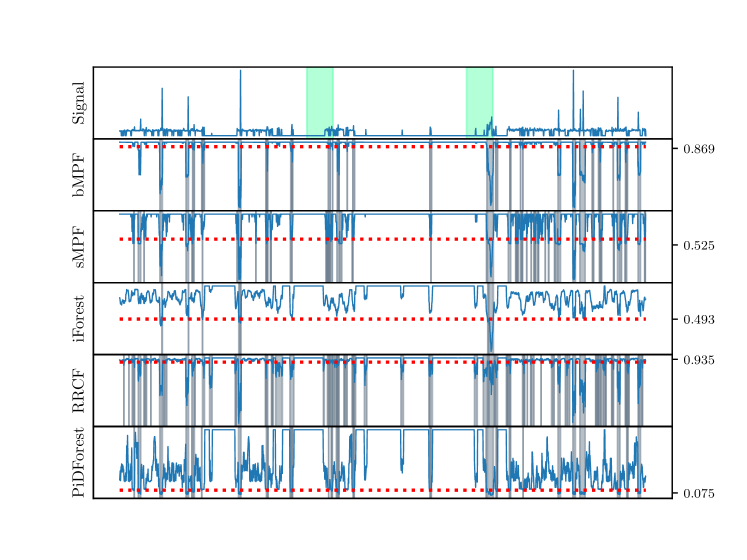
Figure 3: “Rogue_hold” trace denoted by the blue curve in each panel. The top panel illustrates the ground truth anomalies with their associated window in green. Flagged anomalies are in the grey shading and the red dashed line is the threshold which achieves the optimum AUC.

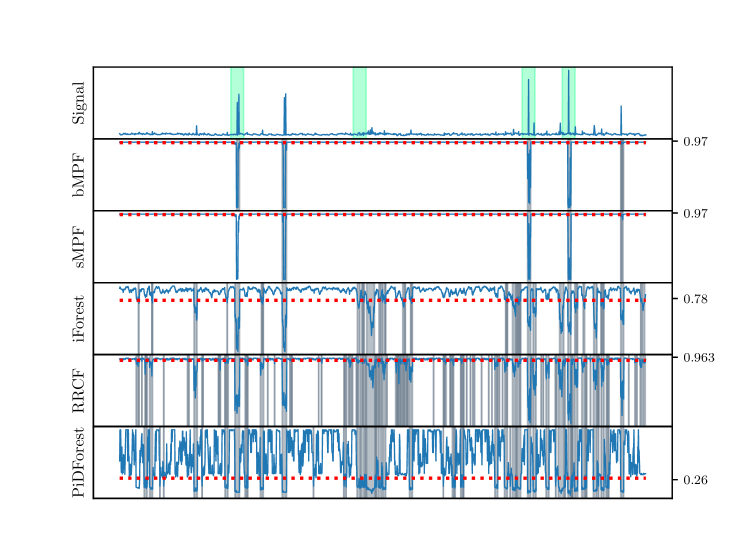
Figure 4: “Ad_exchange” trace. Plots as described in Figure 3

Appendix E Illustrative Examples

E.1 2d Toy Datasets

We provide a simple comparison of the methods on all of the baseline synthetic examples taken from the scikit-learn outlier detection page [3] which contains unimodal and bimodal data. The data is of size $n=500$ which is split between $n_{\text{inliers}}=425$ inlier points and the remaining $n_{\text{outliers}}=75$ being planted outliers chosen uniformly over the input domain. For visual comparison, we plot the resulting classification induced by each of the random forest methods at the optimum threshold. The results are illustrated in Figure 5. We additionally record the area under the ROC curve (AUC) and area under the precision-recall-gain (PRG) curve in Table 9 [15]. Area under a precision-recall curve is not justified, instead use area under the PRG curve. We use [21] to evaluate the Precision-Recall-Gain and observe that again our methods perform well compared to other random forests. These results are presented in Tab. 9 but a more in-depth study is deferred for future work.

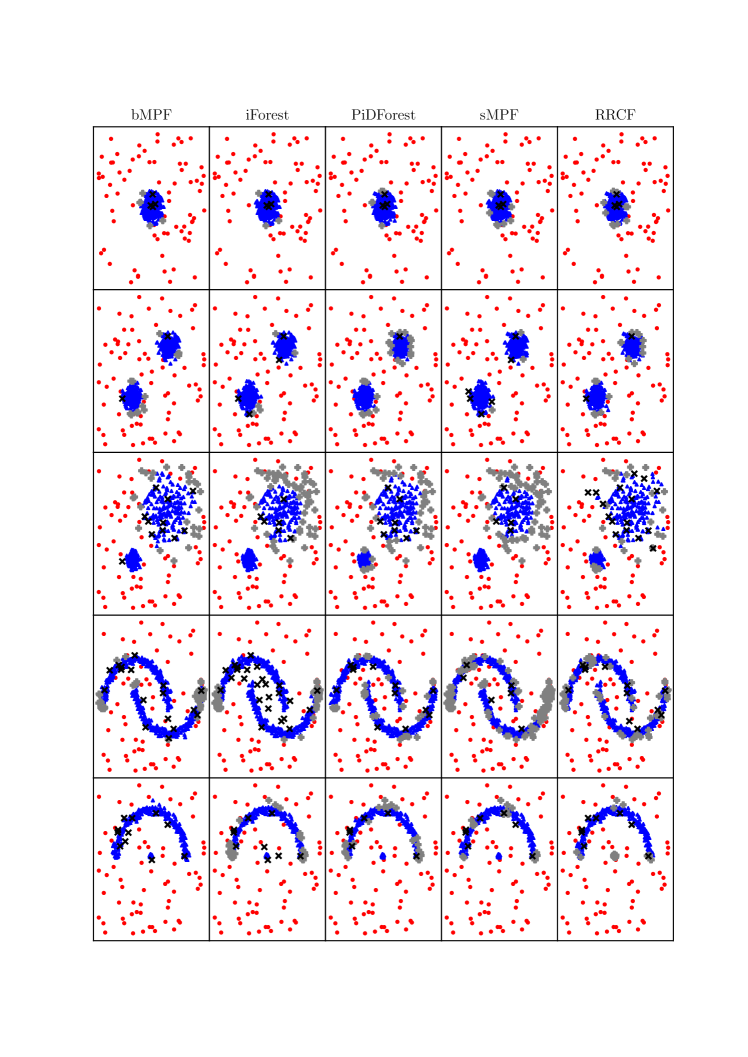
Figure 5: Random Forest Methods on sklearn outlier detection toy datasets. True positives are in red circles, true negatives in blue triangles, false positive in grey $+$, and false negatives in black crosses. Black crosses near the modes are often misclassified by all methods; these correspond to planted anomalies that lie in the normal region.

Dataset	AUC
	sMPF	bMPF	RRCF	iForest	PidForest
Single Blob	0.963	0.966	0.972	0.964	0.963
Two Blobs Tight	0.994	0.994	0.991	0.994	0.993
Two Blobs Spread	0.948	0.956	0.934	0.953	0.960
Moons	0.904	0.901	0.906	0.840	0.914
Moon & Blob	0.977	0.964	0.950	0.955	0.972
	AUPRG
	sMPF	bMPF	RRCF	iForest	PidForest
Single Blob	0.994	0.993	0.991	0.993	0.993
Two Blobs Tight	0.999	0.998	0.998	0.999	0.999
Two Blobs Spread	0.986	0.989	0.982	0.984	0.990
Moons	0.971	0.978	0.976	0.947	0.979
Moon & Blob	0.996	0.997	0.979	0.990	0.994

Table 9: AUC and AUPRG values for Fig. 5

Appendix F Density Estimation

We provide 4 synthetic examples to illustrate the use of our proposed models. A more significant experimental study will be necessary to evaluate the efficacy of the models in this context. The synthetic datasets given below are used to generate an initial sample of 5000 points, after which a grid is placed over the domain to estimate the density. Further investigation is necessary to understand the efficicacy of both Mondrian Pólya Forests as density estimators along with a comparison to popular methods.

1. Standard Normal: Figure 6 (left)

2. Univariate Gaussian Mixture: Figure 6 (right) taken from https://scikit-learn.org/stable/auto_examples/neighbors/plot_kde_1d.html

3. Standard Bivariate Normal: Figure 7 (left)

4. Bivariate Bimodal Mixture: Figure 7 (right). As in the univariate case, except the covariances are adjusted to alter the shape of the clusters. Also the dataset used in Fig. 1.

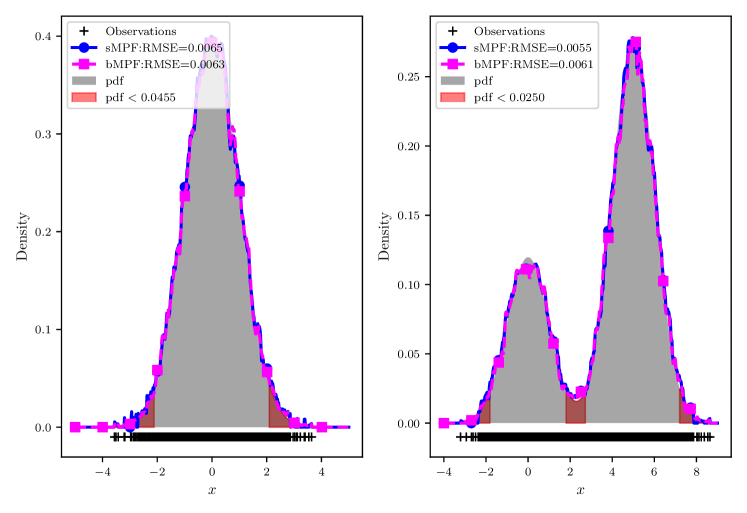
Figure 6: Density estimation on univariate Gaussians

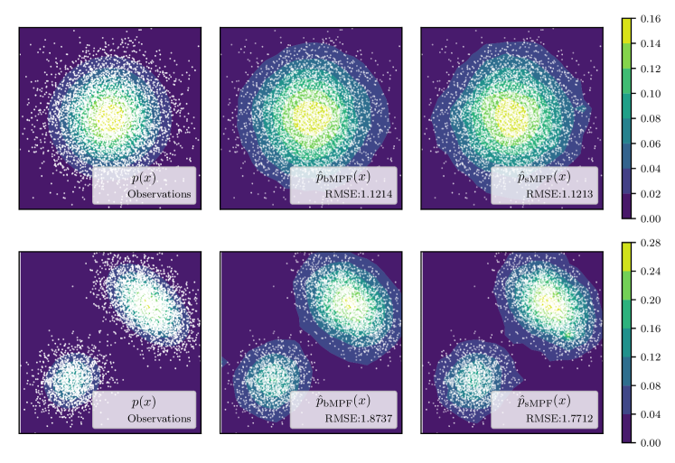
Figure 7: Density estimation on bivariate Gaussians. Left-right: True density function, bMPF, sMPF.

References

- [1] Charu C Aggarwal. Outlier analysis. In Data mining, pages 237–263. Springer, 2015.
- [2] Subutai Ahmad, Alexander Lavin, Scott Purdy, and Zuha Agha. Unsupervised real-time anomaly detection for streaming data. Neurocomputing, 262:134–147, 2017.
- [3] Albert Thomas Alexandre Gramfort. Comparing anomaly detection algorithms for outlier detection on toy datasets. https://scikit-learn.org/stable/auto_examples/miscellaneous/plot_anomaly_comparison.html.
- [4] Fabrizio Angiulli and Clara Pizzuti. Fast outlier detection in high dimensional spaces. In European Conference on Principles of Data Mining and Knowledge Discovery, pages 15–27. Springer, 2002.
- [5] Numenta authors. Numenta anomaly benchmark. https://github.com/numenta/NAB/tree/master/data.
- [6] Matej Balog, Balaji Lakshminarayanan, Zoubin Ghahramani, Daniel M. Roy, and Yee Whye Teh. The Mondrian kernel. In 32nd Conference on Uncertainty in Artificial Intelligence (UAI), June 2016.
- [7] Matej Balog and Yee Whye Teh. The Mondrian process for machine learning. arXiv preprint arXiv:1507.05181, 2015.
- [8] Matthew Bartos, Abhiram Mullapudi, and Sara Troutman. rrcf: Implementation of the Robust Random Cut Forest algorithm for anomaly detection on streams. The Journal of Open Source Software, 4(35):1336, 2019.
- [9] Glencora Borradaile, Brett Burkhardt, and Alexandria LeClerc. Whose tweets are surveilled for the police: An audit of a social-media monitoring tool via log files. In Proceedings of the 2020 Conference on Fairness, Accountability, and Transparency, FAT* ’20, page 570–580, New York, NY, USA, 2020. Association for Computing Machinery.
- [10] Léon Bottou and Chih-Jen Lin. Support vector machine solvers. Large scale kernel machines, 3(1):301–320, 2007.
- [11] Markus M Breunig, Hans-Peter Kriegel, Raymond T Ng, and Jörg Sander. Lof: identifying density-based local outliers. In Proceedings of the 2000 ACM SIGMOD international conference on Management of data, pages 93–104, 2000.
- [12] Graham Cormode, Cecilia Procopiuc, Divesh Srivastava, Entong Shen, and Ting Yu. Differentially private spatial decompositions. In 2012 IEEE 28th International Conference on Data Engineering, pages 20–31. IEEE, 2012.
- [13] Ian Davidson and Selvan Suntiha Ravi. A framework for determining the fairness of outlier detection. In Proceedings of the 24th European Conference on Artificial Intelligence (ECAI2020), 2029.
- [14] Tom Diethe, Tom Borchert, Eno Thereska, Borja de Balle Pigem, and Neil Lawrence. Continual learning in practice. In NeurIPS 2018 Workshop on Continual Learning, 2018.
- [15] Peter Flach and Meelis Kull. Precision-recall-gain curves: Pr analysis done right. In Advances in neural information processing systems, pages 838–846, 2015.
- [16] Parikshit Gopalan, Vatsal Sharan, and Udi Wieder. Pidforest: anomaly detection via partial identification. In Advances in Neural Information Processing Systems, pages 15783–15793, 2019.
- [17] Sudipto Guha, Nina Mishra, Gourav Roy, and Okke Schrijvers. Robust random cut forest based anomaly detection on streams. In International conference on machine learning, pages 2712–2721, 2016.
- [18] Balaji Lakshminarayanan. Decision trees and forests: a probabilistic perspective. PhD thesis, UCL (University College London), 2016.
- [19] Balaji Lakshminarayanan, Daniel M Roy, and Yee Whye Teh. Mondrian forests: Efficient online random forests. In Advances in neural information processing systems, pages 3140–3148, 2014.
- [20] Fei Tony Liu, Kai Ming Ting, and Zhi-Hua Zhou. Isolation forest. In 2008 Eighth IEEE International Conference on Data Mining, pages 413–422. IEEE, 2008.
- [21] Miquel Perello Nieto Meelis Kull, Telmo de Menezes e Silva Filho. pyprg: Python package for creating precision-recall-gain curves and calculating area under the curve. https://github.com/meeliskull/prg/tree/master/Python_package.
- [22] Peter Müller, Abel Rodriguez, et al. Pólya trees. In Nonparametric Bayesian Inference, pages 43–51. IMS and ASA, 2013.
- [23] F. Pedregosa, G. Varoquaux, A. Gramfort, V. Michel, B. Thirion, O. Grisel, M. Blondel, P. Prettenhofer, R. Weiss, V. Dubourg, J. Vanderplas, A. Passos, D. Cournapeau, M. Brucher, M. Perrot, and E. Duchesnay. Scikit-learn: Machine Learning in Python . Journal of Machine Learning Research, 12:2825–2830, 2011.
- [24] Sridhar Ramaswamy, Rajeev Rastogi, and Kyuseok Shim. Efficient algorithms for mining outliers from large data sets. In Proceedings of the 2000 ACM SIGMOD international conference on Management of data, pages 427–438, 2000.
- [25] Shebuti Rayana. ODDS library. http://odds.cs.stonybrook.edu, 2016.
- [26] Daniel M Roy, Yee Whye Teh, et al. The Mondrian process. In NIPS, pages 1377–1384, 2008.
- [27] Bernhard Schölkopf, John C Platt, John Shawe-Taylor, Alex J Smola, and Robert C Williamson. Estimating the support of a high-dimensional distribution. Neural computation, 13(7):1443–1471, 2001.
- [28] Vatsal Sharan. PIDForest library. https://github.com/vatsalsharan/pidforest, 2019.
- [29] Mei-Ling Shyu, Shu-Ching Chen, Kanoksri Sarinnapakorn, and LiWu Chang. A novel anomaly detection scheme based on principal component classifier. Technical report, Miami University Department of Electrical and Computer engineering, 2003.
- [30] Joaquin Vanschoren, Jan N. van Rijn, Bernd Bischl, and Luis Torgo. OpenML: Networked science in machine learning. SIGKDD Explorations, 15(2):49–60, 2013.
- [31] Yue Zhao, Zain Nasrullah, and Zheng Li. PyOD: A Python toolbox for scalable outlier detection. Journal of Machine Learning Research, 20(96):1–7, 2019.