ACT-04-20

MI-TH-2015

Primordial Black Holes from No-Scale Supergravity

Dimitri V. Nanopoulos¹, Vassilis C. Spanos², Ioanna D. Stamou²

¹George P. and Cynthia W. Mitchell Institute for Fundamental Physics and Astronomy, Texas A&M University, College Station, Texas 77843, USA;
Astroparticle Physics Group, Houston Advanced Research Center (HARC),
Mitchell Campus, Woodlands, Texas 77381, USA;
Academy of Athens, Division of Natural Sciences, Athens 10679, Greece

²National and Kapodistrian University of Athens, Department of Physics,
Section of Nuclear & Particle Physics, GR–15784 Athens, Greece

We calculate the primordial black hole abundance in the context of a Wess-Zumino type no-scale supergravity model. We modify the Kähler potential, by adding an extra exponential term. Using just one parameter in the context of this model, we are able to satisfy the Planck cosmological constraints for the spectral index $n_{s}$, the tensor-to-scalar ratio $r$, and to produce up to $\sim 20\%$ of the dark matter of the Universe in the form of primordial black holes.

1 Introduction

The recent observations of black hole (BH) mergers by VIRGO/LIGO open a new window to probe BH physics [1, 2, 3, 4, 5]. These detections rekindled the idea that Primordial Black Holes (PBH) can be considered as Dark Matter (DM) candidates [6, 7, 8]. As the nature of DM remains one of the most notable mysteries in physics, a flurry of activity has recently taken place in this direction [9, 10, 11, 12, 13, 14, 15, 16, 17, 18, 19, 20, 21, 22, 23, 24, 25, 26, 27, 28, 29, 30, 31, 32, 33, 34, 35, 36].

It has been proposed that a spike in the Cosmic Microwave Background (CMB) power spectrum can be physically significant, as it could lead to formation of PBHs. Such a spike is related to an inflection point in the scalar inflaton potential  [16]. In the context of single field inflation models, an inflection point is created whence the slow-roll parameter $\varepsilon$, that is related to the derivative of the inflaton, gets sizeable value. On the other hand, $\varepsilon$ stays below one, allowing the inflation to goes on. The local enhancement supervened by a period where the inflaton is almost constant. During this plateau the power spectrum amplifies, enabling production of PBH in the radiation dominated phase of the early universe. This PBH abundance can be interpreted as a substantial fraction of the DM of the Universe. Similar reinforcement in the power spectrum can be achieved in the context of two-field models [21, 33]. In these models, one field plays the role of the inflaton and the other is responsible for the PBH production.

It is now clear, that a more precise calculation of the power spectrum is indispensable. This evaluation can be achieved by solving numerically the so-called Mukhanov-Sasaki (M-S) equation [37, 38]. Because the slow-roll approximation fails to reproduce the exact results in many proposed models, such as the one in ref.[9], it is imperative to solve the M-S equation exactly. In addition to that, the precise size and the location of the peak of the power spectrum is crucial for calculating the fractional abundance of PBH in the Universe.

Here, we try to sum up the basic developments in PBH production using single field inflation. Specifically, in [9] the authors employ a model based on an effective potential with an approximate inflection point, arise from two-loop logarithmic corrections. In [10, 14] it has been considered the PBH production studying a string inflation model. Alternatively, models in (critical) Higgs inflation has been studied in  [17, 20]. A power spectrum by a polynomical potential has been suggested in [16, 19, 18]. In [13, 27] has been proposed a supergravity model with a single chiral field. Moreover, the authors in [15, 30] have studied inflationary $\alpha$-attractor models. Finally, PBH by axion monodromy has been considered in [32].

Embedding models of inflation, into a more fundamental quantum theory such as supergravity, results to a framework that can be predictive and reveals an aspect of the high energy scale [39]. Taking this into account, we consider that the natural framework for formulating models of inflation is supergravity. Specifically, no-scale supergravity models [39, 40, 41, 42, 43], turn out to have other advantages: their potential depends on a minimal number of parameters, they evade the $\eta$ problem and they emerge naturally as the low energy limit of compactified string models [44]. In principle, no-scale models are necessarily multifield inflation models. This means that apart from the inflaton, there are additional scalar fields (moduli).

In this paper, we introduce an inflationary model based on the no-scale supergravity [45]. Specifically, we consider models with Starobinsky-like potential, derived by no-scale supergravity theories. Since, we need to study the formation of PBHs within these models, we deform the ordinary $SU(2,1)/SU(2)\times U(1)$ Kähler potential, in order to achieve acceptable fluctuations to the scalar inflaton potential, producing an inflection point. For this reason we introduce an exponential term with one extra parameter. We have paid particular attention to satisfy all the Planck cosmological constraints throughout our numerical analysis. As a result we have found models that satisfying all the phenomenological constraints, can produce up to 20% of the total DM of the Universe, due to PBH formation. This value almost saturates the allowed range for the PBH abundance, applying all the relevant observational data.

The layout of the paper is as follows: In section 2 we briefly review some basic aspects of supergravity, relevant to inflation. In section 3 we modify the Kähler potential and we calculate the effective scalar potential by fixing the noncanonical kinetic terms. We choose the inflationary direction and we verify that it remains stable. Moreover, we solve the background equation and we justify the insufficiency of the slow-roll approximation. Therefore, we describe an algorithm for the numerical solution of M-S equation. Using these solutions we estimate the fractional DM abundance of the PBH as a function of its mass and we delineate the phenomenologically accepted regions on this parameter space. Finally, in section 4 we give our conclusions and perspectives.

2 Supergravity models and inflation

The most general $N=1$ supergravity theory is characterized by three functions. The Kähler potential $K$, which is a Hermitian function of the matter scalar field $\Phi^{i}$ and describes its geometry, a holomorphic function of the fields, called superpotential $W$ and a holomorphic function $f_{ab}$.

In the following, we set the reduced Planck mass $M_{P}=(8\pi G)^{-1/2}$ to unity. The $N=1$ supergravity action can be written as:

$$\mathcal{S}=\int d^{4}x\sqrt{-g}\left(K_{i\bar{j}}\partial_{\mu}\Phi^{i}\partial^{\mu}\bar{\Phi}^{\bar{j}}-V\right).$$ (1)

Given the Kähler potential $K$ and the superpotential $W$, one can obtain the real field metric $K_{i\bar{j}}$ and the scalar potential $V$, following the procedure outlined below.

The general form of field metric reads as

$$K_{i\bar{j}}(\Phi,\bar{\Phi})=\frac{\partial^{2}K}{\partial\Phi^{i}\partial\bar{\Phi}^{\bar{j}}}\,.$$ (2)

Moreover, the scalar potential is given by

$$V=e^{K}\left(K^{i\bar{j}}\mathcal{D}_{i}W\mathcal{D}_{\bar{j}}\bar{W}-3|W|^{2}\right)+\frac{\tilde{g}^{2}}{2}(K^{i}T^{a}\Phi_{i})^{2}\,,$$ (3)

where $K^{i\bar{j}}$ is the inverse Kähler metric and the covariant derivatives are defined as:

$$\mathcal{D}_{i}W\equiv\partial_{i}W+K_{i}W$$ (4)

$$\mathcal{D}^{i}W\equiv\partial^{i}W-K^{i}W\,.$$

In addition, we have defined that $K_{i}\equiv\partial K/\partial\Phi^{i}$ and, correspondingly, the complex conjugate $K^{i}$. The last term in the scalar potential (3) is just the $D$-term potential, which is set to zero, since the fields $\Phi_{i}$ are gauge singlets. From (1) is clear that the kinetic term $\mathcal{L}_{KE}=K_{i\bar{j}}\partial_{\mu}\Phi^{i}\partial^{\mu}\bar{\Phi}^{\bar{j}}$ needs to be fixed.

The minimal no-scale $SU(1,1)/U(1)$ model is written in the terms of a single complex scalar field $T$, with the Kähler potential [40]

$$K=-3\ln\left(T+\bar{T}\right)\,.$$ (5)

In our case, we consider a no-scale supergravity model with two chiral superfields $T$, $\varphi$, that parametrize the noncompact $SU(2,1)/SU(2)\times U(1)$ coset space. In this model, the Kähler potential can be written as [42]

$$K=-3\ln\left(T+\bar{T}-\frac{\varphi\bar{\varphi}}{3}\right)\,.$$ (6)

Then, the corresponding action (1) becomes:

$$\mathcal{S}=\int d^{4}x\sqrt{-g}\left[\frac{1}{2}(\partial_{\mu}\varphi,\partial_{\mu}T)\left(\begin{array}[]{cc}K_{\varphi\bar{\varphi}}&K_{\varphi\bar{T}}\\ K_{T\bar{\varphi}}&K_{T\bar{T}}\\ \end{array}\right)\left(\begin{array}[]{c}\partial^{\mu}\varphi\\ \partial^{\mu}T\\ \end{array}\right)-V(\varphi,T)\right].$$ (7)

The simplest globally symmetric model is the Wess-Zumino model, with a single chiral superfield $\varphi$. This model is characterized by a mass term $\hat{\mu}$ and a trilinear coupling $\lambda$. Thus, the superpotential is given by [45]

$$W=\frac{\hat{\mu}}{2}\varphi^{2}-\frac{\lambda}{3}\varphi^{3}.$$ (8)

It is possible to embed this model in the context of the no-scale $SU(2,1)/SU(2)\times U(1)$ case, by matching the $T$ field to the modulus field and the $\varphi$ to the inflaton field. By doing so, one can derive from (6) and (8) a class of no-scale models that yield Starobinsky-like effective potentials. This potential is calculated along the real inflationary direction defined by

$$T=\bar{T}=\frac{c}{2}\,\,,\quad\mathrm{Im}\varphi=0\,,$$ (9)

with the choice $\lambda/\mu=1/3$ and $\hat{\mu}=\mu\sqrt{c/3}$, where $c$ is a constant.

In order to have canonical kinetic terms, the field $\varphi$ has to be transformed [45] as

$$\varphi=\sqrt{3\,c}\,\tanh\left(\frac{\chi}{\sqrt{3}}\right)\,,$$ (10)

recovering the potential of the Starobinsky model

$$V(\chi)=\frac{\mu^{2}}{4}\left(1-e^{-\sqrt{\frac{2}{3}}\,{\chi}}\right)^{2}\,.$$ (11)

In Fig. 1, we plot the potential derived from the superpotential Eq. (8) that depends on the ratio $\lambda/\mu$, for various values of this ratio around $1/3$. This central value corresponds to the Starobinsky case. In order to comply with the cosmological data [46, 47, 48] and to explore the dependence on the total number of e-folds, we vary the parameter $\mu$ in the range ($1.8$– $3.4$)$\times\,10^{-5}$.

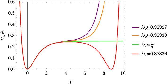
Figure 1: The potential as given by Eqs. (8) and (10) for various values of the ratio $\lambda/\mu$, as in [45].

Studying no-scale models with two chiral superfields $\varphi$ and $T$, we notice that these fields can interchange roles as the inflaton and modulus [45, 49]. In the case which $\varphi$ is the modulus field and $T$ is the inflaton, the superpotential reads as [49, 50]

$$W=\mu\,\varphi\,\left(T-\frac{1}{2}\right)\,.$$ (12)

The Starobisky potential is recovered along the inflationary direction $\varphi=\bar{\varphi}=\mathrm{Im}T=0$ and $\mathrm{Re}T=\phi$. In this case too, in order to have canonical kinetic term, one needs to transform the field $\phi$ to $\chi$ using a relation similar to (10). Hence, the effective scalar potential is also given by Eq. (11).

It is essential one to verify that the masses of the inflaton and the modulus field are not tachyonic. Thus, before calculating the evolution of the field, we must check the stabilization along the inflationary direction. If the stabilization is achieved, the modulus field can be set to be zero and the relevant term becomes irrelevant to the dynamical evolution of the inflaton.

3 Calculating PBH from the modified Kähler potential

In this section, we will study modifications of the Kähler potential, that induce an inflection point to the scalar potential, and consequently causes peaks in the CMB power spectrum. For this reason, we use as basis the Wess-Zumino potential (8), modifying the Kähler potential, by introducing an exponential term as

$$K=-3\ln\left[T+\bar{T}-\frac{\varphi\bar{\varphi}}{3}+a\,e^{-b(\varphi+\bar{\varphi})^{2}}(\varphi+\bar{\varphi})^{4}\right]\,,$$ (13)

where $a$ and $b$ are real numbers. Obviously, in the limit $a=0$, we retrieve the result that corresponds to the Starobinsky potential, as calculated in the previous section. Moreover, expanding the exponential, one obtains a polynomial modification of the Kähler potential, as it has been used in the literature [16, 19, 18]. The particular exponential form has the advantage that practically introduces just one extra parameter, $b$. In our analysis the parameter $a$ gets just two values: $a=0$ to switch off the effect of the modified term and $a=-4$ when the extra term is used.

The real part of the field $\varphi$ plays the role of the inflaton. In order to verify the stability of the potential, along the real direction in Eq.  (9), we calculate the squared mass matrix and we check that no tachyonic instability is present, that is $m^{2}_{\mathrm{Re}T},m^{2}_{\mathrm{Im}T},m^{2}_{\mathrm{Im}\varphi}\geq 0$.

In detail, the general form of mass matrix is

$$m^{2}_{s}=\begin{pmatrix}(K^{-1})^{i}_{k}\mathcal{D}^{k}\partial_{j}V&(K^{-1})^{i}_{k}\mathcal{D}^{k}\partial^{j}V\\ (K^{-1})^{k}_{i}\mathcal{D}_{k}\partial_{j}V&(K^{-1})^{k}_{i}\mathcal{D}_{k}\partial^{j}V\end{pmatrix}\,,$$ (14)

where $(K^{-1})^{i}_{j}$ is the inverse metric of $K^{j}_{i}=\partial^{2}K/\partial\Phi^{i}\partial\Phi_{j}$ and the Kähler covariant derivative is given in (4). Specifically, in the case of the two chiral fields the mass matrix takes the form

$$m^{2}_{s}=\begin{pmatrix}(K^{-1})^{\varphi}_{k}\mathcal{D}^{k}\partial_{\varphi}V&(K^{-1})^{\varphi}_{k}\mathcal{D}^{k}\partial^{\bar{T}}V\\ (K^{-1})^{k}_{{T}}\mathcal{D}_{k}\partial_{\bar{\varphi}}V&(K^{-1})^{k}_{\bar{T}}\mathcal{D}_{k}\partial^{\bar{T}}V\end{pmatrix}.$$ (15)

Following [51, 52], we have computed analytically and numerically the masses of the fields $\varphi$ and $T$ and we have verified that along the real direction, $T=\bar{T}$ and $\varphi=\bar{\varphi}$, the eigenstates of the matrix (15) are positive. Unfortunately, the corresponding equations are too long to be displayed here. Repeating the same calculation in the imaginary direction, we have checked the positivity of the mass eigenstates, using $\left\langle\mathrm{Re}T\right\rangle=\frac{c}{2}$ and $\left\langle\varphi\right\rangle=0$.

Having verified the stability along the inflationary direction, using Eqs. (2),(3), the scalar effective potential can be calculated. As a first step, we find the field transformation, that puts the kinetic term in canonical form. Moreover, defining $\mathrm{Re}\,\varphi\equiv\,\phi$, the relevant term in Eq. (7) is the $K_{\varphi\bar{\varphi}}$, which along the direction (9), apparently equals to $K_{\phi\phi}$. Thus, one gets

$$\frac{1}{2}\,\partial_{\mu}\chi\,\partial^{\mu}\chi=K_{\phi\phi}\,\partial_{\mu}\phi\,\partial^{\mu}\phi\,$$ (16)

or equivalently

$$\frac{d\chi}{d\phi}=\sqrt{2K_{\phi\phi}}\,.$$ (17)

By integrating the latter, we obtain the generalization of Eq. (10), using appropriate boundary conditions. These conditions are fixed from the requirement to retrieve the Strarobinsky case, in the limit $a=0$.

Afterwards, we compute the scalar potential along the direction (9), using Eq. (3) and the modified Kähler potential from (13), as

$$V(\phi)=\frac{3e^{3b\phi^{2}}\phi^{2}(c\mu^{2}-2\sqrt{3c}\lambda\,\mu\,\phi+3\lambda^{2}\,\phi^{2})}{\left[-3a\phi^{4}+e^{b\phi^{2}}(-3c+\phi^{2})\right]^{2}\,\left[e^{b\phi^{2}}-6\,a\,\phi^{2}(6+b\,\phi^{2}(-9+2b\,\phi^{2}))\right]}\,.$$ (18)

Finally, using the generalized relation $\phi(\chi)$, obtained by Eq. (17), the potential above can be expressed as $V(\chi)$. The precise form of the $V(\chi)$ is obtained only numerically, due to its complexity and this numerical relation is used thereafter.

	$\lambda/\mu$	$b$
1.	$0.33327$	$87.379427$
2.	$0.33330$	$87.390563$
3.	$1/3$	$87.402941$

Table 1: The values of the parameters $\lambda/\mu$ and $b$, for $a=-4$ and $2\left\langle\mathrm{Re}T\right\rangle=c=0.065$.

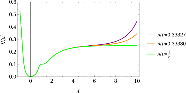
Figure 2: The potential given in Eq. (18) as a function of $\chi$, for various values of the ratio $\lambda/\mu$ as in Table 1.

In Fig. 2 we plot the potential $V(\chi)/\mu^{2}$, as a function of the field $\chi$, using the values of the parameters $\lambda/\mu$ and $b$, as in Table 1. The parameter $\mu$ is fixed in order to satisfy the Planck constraint for power spectrum, which is approximately $P_{\mathcal{R}}=2.1\times 10^{-9}$, at a pivot scale of $k_{*}=0.05\,\mathrm{Mpc}^{-1}$. As we will discuss below, varying the parameter $\lambda$ affects mainly the spectral index $n_{s}$, but also the tensor-to-scalar ratio $r$ of the power spectra. After fixing $\lambda$ and $\mu$, the values for $b$ in Table 1, are chosen in order the PBH abundance to saturate the cosmological bounds. which as we will see, constrain significantly the parameter space of the PBH. The prediction of the model is not very sensitive on the $a$, and thus is chosen to be $a=-4$. Finally, in the context of our model, the parameter $c$ affects mainly the total number of e-folds. To get agreement with the Planck 2018 data we choose $c=0.065$.

One can notice, that the potential has the required features that ensure that sizable abundance of PBH is created. Specifically, the potential around the inflection point $\chi\sim 1$, satisfies the relations

$$\frac{dV(\chi_{i})}{d\chi_{i}}\simeq 0,\quad\frac{d^{2}V(\chi_{i})}{d\chi_{i}^{2}}=0\,.$$

Around the inflection point, the inflaton slows down, generating a large amplification in the power spectrum. In addition, it has a minimum with $V(\chi_{0})=0$, at $\chi_{0}=0$, to achieve the reheating, after inflation ends.

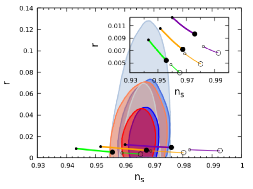
Figure 3: The predictions of our model for the tilt $n_{s}$ and the tensor-to-scalar ratio $r$. The shaded regions are taken from Planck 2018 and other data [46]. For the details see the main text.

In Fig. 3 we plot the predictions for the tilt $n_{s}$ in the spectral index of scalar perturbations and for the tensor-to-scalar ratio $r$, of the original Wess-Zumino model (thin line segments with empty dots) and the model with modified Kähler potential (thick line segments with filled dots), compared against the recent data of Planck 2018, that prefer the central shaded regions in the plot. The meaning of the colors of these regions are explained in the Planck collaboration analysis [46]. Green colored lines correspond to the case $\lambda/\mu=1/3$, the orange to $0.33330$ and the purple to $0.33327$. The evolution of the field is fixed by requiring 50 (small dots), or 60 (big dots) e-folds at the end of the line segments. We notice, that introducing the modified potential in Eq. (13), the cosmological predictions are affected considerably. Therefore, some values of the ratio $\lambda/\mu$, which were originally excluded, become acceptable in the modified case.

3.1 Applying the slow-roll approximation

The evolution of the inflaton field $\chi$ in a Friedmann–Robertson–Walker (FRW) homogeneous background, which we take to be spatially flat, is driven by the system of the Friedmann equation and the inflaton field equation:

$$\begin{split}H^{2}=\frac{1}{3}\left(\frac{1}{2}\dot{\chi^{2}}+V(\chi)\right)\\ \ddot{\chi}+3H\dot{\chi}+V^{\prime}(\chi)=0\,,\end{split}$$ (19)

where dots represent derivatives with respect to cosmic time and primes the derivatives with respect to the field $\chi$. We can rewrite the system above in terms of number of e- folds elapsed from initial cosmic time $t_{i}$ described by the integral:

$N(t)=\int^{t}_{t_{i}}H(t^{\prime})dt^{\prime}$.

So, the background equation or the equation of the inflaton field take the form

$$\frac{d^{2}\chi}{dN^{2}}+3\frac{d\chi}{dN}-\frac{1}{2}\left(\frac{d\chi}{dN}\right)^{3}+\left[3-\frac{1}{2}\left(\frac{d\chi}{dN}\right)^{2}\right]\frac{d\ln V(\chi)}{d\chi}=0.$$ (20)

We solve numerically the Eq. (20), using as initial conditions those that, in the slow-roll approximation are compatible with the cosmologically acceptable values for $n_{s}$ and $r$ [47, 46, 48]. Specifically, by the Planck 2018 data [46] on inflationary parameters, at the pivot scale $k_{*}=0.05\,\mathrm{Mpc}^{-1}$, we get

$$\begin{array}[]{cc}n_{s}=0.9625\pm 0.0048\\ r<0.044.\end{array}$$ (21)

We evaluate the spectral index $n_{s}$ and the tensor-to-scalar ratio $r$, at leading order in the slow-roll expansion by

$$n_{s}\simeq 1+2\eta_{V}-6\varepsilon_{V},\quad r\simeq 16\varepsilon_{V}\,,$$ (22)

where the relevant slow-roll parameters are defined as

$$\varepsilon_{V}=\frac{1}{2}\left(\frac{V^{\prime}(\chi)}{V(\chi)}\right)^{2},\quad\eta_{V}=\frac{V^{\prime\prime}(\chi)}{V(\chi)}.$$ (23)

Using the numerical relation between $\phi$ and $\chi$, based on Eq. (17), the initial condition for the field $\phi$ can be transformed to the initial conditions for the $\chi$. As for the initial condition for the derivative of $\chi$, we use the slow-roll attractor relation

$$\frac{d\chi}{dN}\approx-\left|{\frac{dV}{Vd\chi}}\right|\,.$$ (24)

Consequently, the numerical solution for the slow-roll parameters reads as

$$\varepsilon_{H}=\frac{1}{2}\left(\frac{d\chi}{dN}\right)^{2},\quad\eta_{H}=\varepsilon_{H}-\frac{1}{2}\frac{d\ln\varepsilon_{H}}{dN}.$$ (25)

Using this equation for $\varepsilon_{H}$, the Hubble function squared reads from Eq. (19) as

$$H^{2}=\frac{V(\chi)}{3-\varepsilon_{H}}.$$ (26)

Given these expressions, we evaluate the power spectrum within the slow-roll approximation, as:

$$P_{\mathcal{R}}\simeq\frac{1}{8\pi^{2}}\frac{H^{2}}{\varepsilon_{H}}.$$ (27)

Notice that for the numerical solution of the background Eq. (20), one must use the Eq. (17) and Eq. (18). As usual, the condition $\varepsilon_{H}\approx 1$ marks the end of inflation and the numerical calculation ends at this point. We constrain the number of e-folds $N$, that is the number of e-folds elapsed between the time that today’s largest observable scales exit the Hubble horizon and the time at which inflation ends, to be $45-55$.

	$\phi_{0}$	$\lambda/\mu$	$n_{s}$	$r$
1.	$0.4258$	$0.33327$	$0.961234$	$0.0121106$
2.	$0.4272$	$0.33327$	$0.967463$	$0.0109205$
3.	$0.4266$	$0.33330$	$0.958265$	$0.00900217$
4.	$0.4258$	$1/3$	$0.948072$	$0.00740699$

Table 2: The initial conditions for the field $\phi$, $n_{s}$ and $r$ that correspond to sets in Table 1. (The first two sets correspond to the first set of Table 1, with different $\phi_{0}$.)

In our numerical analysis, we use the sets of parameters given in Table 1, as discussed in the beginning of this section. For the initial condition of the field $\phi$, $\phi_{0}$, we use the numbers in the first column in Table 2. Please note that, the first two lines in Table 2, correspond to the first line in Table 1. The last two columns in Table 2 are the outcome of the calculation, the predicted values for the observables $n_{s}$ and $r$. The initial conditions $\phi_{0}$ and $N_{*}=0$ are set to the point that CMB scales cross the horizon. In addition, this point corresponds to the asymptotic plateau of the potential $V(\chi)$ in Fig. 2. At the end of this procedure, we calculate the evolution of the field $\chi$ and the slow-roll parameters $\varepsilon_{H}$, $\eta_{H}$ in terms of $N$, and show our results in Figs. 4 left and right panel, respectively.

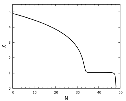
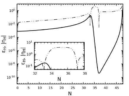
Figure 4: Left panel: The evolution of the inflaton field $\chi$, in Planck units, as a function of the numbers of e-folds. Right panel: The slow-roll parameters using the first set of parameters in Table 1. Solid line corresponds to $\varepsilon_{H}$ and dashed to $|\eta_{H}|$.

As it can be seen in Fig. 4 right, the value of parameter $\varepsilon_{H}$ remains always below 1 until the end of inflation. We further notice that the inflaton reaches the region of reheating at the global minimum of potential in Fig. 2, that corresponds to $N\simeq 50$ in Fig. 4 left, as it was expected.

Using the slow-roll approximation for calculating the power spectrum as in Eq. (27), we can get sizable peaks. However, paying attention to the details of the slow-roll approximation, especially to the values of the parameters $\varepsilon_{H}$ and $\eta_{H}$ in Fig. 4 right, we remark that they get values of $\mathcal{O}(10^{-1})$–$\mathcal{O}(1)$, that clearly violate this approximation. Therefore, it is crucial to solve the precise M-S equation and then we can proceed to the evaluation of fractional abundance of PBH.

3.2 Solving the Mukhanov-Sasaki equation

As it has been explained in the previous section the slow-roll approximation fails to reproduce the correct power spectrum and hence the correct mass of PBH as well as, the fractional abundances. The fact that the values of slow-roll parameters $\varepsilon_{H}$ and $\eta_{H}$ are close to 1 and over 3 respectively, leads us to search for a more accurate method. When the potential has a sharp feature such as an inflection point, it is crucial to evolve the full mode equation numerically, without any approximation [53]. Hence, we need to have an precise solution of the power spectrum, versus the comoving wave-number $k$ in order to produce the abundance of PBH. This solution can be found by the so-called M-S equation[37, 38] which is given by the following expression:

$$\frac{d^{2}u_{k}}{dN^{2}}+(1-\varepsilon_{H})\frac{du_{k}}{dN}+\left[\frac{k^{2}}{\mathcal{H}^{2}}+(1+\varepsilon_{H}-\eta_{H})(\eta_{H}-2)-\frac{d(\varepsilon_{H}-\eta_{H})}{dN}\right]u_{k}=0$$ (28)

and

$$u=zR,\quad z=\frac{a}{\mathcal{H}}\frac{d\phi}{d\tau},$$ (29)

where $R$ is the comoving curvature perturbation and $a$ is the scale factor. We denote by $\tau$ the conformal time and by $\mathcal{H}=aH$ the conformal Hubble parameter. Instead of working with complex coefficients, it is convenient to solve the M-S equation twice: one for the real and one for the imaginary part for each mode $u_{k}$. The corresponding initial conditions are [53]:

$$\mathrm{Re}\left(u_{k}\right)=\frac{1}{\sqrt{2k}}\,,\quad\mathrm{Im}\left(u_{k}\right)=0$$ (30)

$$\mathrm{Re}\left(\frac{du_{k}}{dN_{i}}\right)=0,\quad\mathrm{Im}\left(\frac{du_{k}}{dN_{i}}\right)=-\frac{\sqrt{k}}{\sqrt{2}k_{i}}$$

where $k_{i}$ is chosen a thousand times smaller than the wave-number of interest. To evaluate the power spectrum we repeat the integration over many values of $k$. The numerical precise value of spectrum (solving the M-S equation) is given by:

$$P_{\mathcal{R}}=\frac{k^{3}}{2\pi^{2}}{\Big{|}{\frac{u_{k}}{z}\Big{|}^{2}}}_{k\ll\mathcal{H}}.$$ (31)

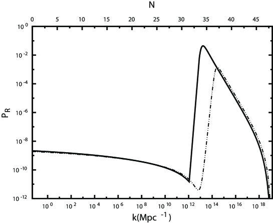
Figure 5: The CMB power spectrum using the slow-roll approximation (dashed line) and the M-S formalism (solid line) for the first set of parameters of Table 1.

The numerical strategy for solving the M-S equation, based on refs. [9, 30], is summarized below:

• The background Eq. (20) is solved numerically using the initial conditions for the field and its first derivative. The numerical solution stops when the condition $\varepsilon_{H}=1$ is satisfied, denoting the end of inflation. The total number of e-folds is defined between the times where the $k$-modes exit and enter the Hubble horizon. The transformation of the field needs to be taken into account too.

• In order to solve the Eq. (28) the solution of the background equation for $\chi$ is required, as well as the slow-roll parameters from the previous steps. The second and third derivatives of $\chi$ in the last term of (28) are also be evaluated using Eq. (20) and its first derivative with respect to $N$.

• One can now solve the M-S equation. For each mode of interest $k$, the Eq. (28) is solved twice with the initial conditions given by (30), until the solution is approximately constant ($\frac{u_{k}}{z}\approx const$). We choose the values of initial $N_{i}$ to be $N=N_{i}-N_{*}$ and the connection between the number of e-folds and the comoving wave-number is given by:

  $$k=k_{*}\frac{H(N_{i})}{H(N_{*})}e^{N_{i}-N_{*}}\,.$$ (32)

  The initial value of $k_{*}$ is $k_{*}=0.05\,\mathrm{Mpc}^{-1}$ and we assume that $N_{*}=0$, as the CMB scales exit the Hubble horizon.

• Eventually, the $P_{\mathcal{R}}$ is evaluated precisely using Eq. (31) for each $k$-mode of interest, which is related to $N$ as it is explained in the previous step. As for the normalization of the power spectrum we use that it is approximately $2.1\times 10^{-9}$ [48] at $k_{*}=0.05\,\mathrm{Mpc}^{-1}$.

With this algorithm we are able to reproduce previous works, such as those of refs.[9, 10, 13, 14]. This numerical method is applied to our case, where the Kähler potential is modified. The power spectrum is evaluated using Eqs. (28) and (31) and depicted in Fig. 5 for the first set of parameters shown in Table 1 taking into consideration that the initial condition for the background equation is given by the first set of Table 2. The solid line corresponds to the M-S power spectrum and the dashed line to the slow-roll approximation as in Eq. (27). As one can notice in Fig. 5, despite the fact that peaks can be produced within the slow-roll approximation, this approximation fails to reproduce either the peak’s height or its position. The numerical precise result of power spectrum ensures that the value of peak’s height is larger than $10^{-2}$ and hence a significant fractional abundance of PBH can be achieved, as it is shown in the next section.

We notice that employing improvements of the slow-roll approximation like the optimized slow-roll approximation [24], the size of power spectrum peak, approaches indeed this of the M-S numerical solution. On the other hand, although using either the slow-roll or its improvement, the peak’s position is not affected, this is quite different from this of the numerical solution. As it will be discussed below, since the position of the peak is crucial for the precise calculation of fractional PBH abundance, in the following we will use the M-S numerical solution, as it is suggested in [22].

3.3 The calculation of the PBH abundance

Using the precise calculation of the power spectrum via the M-S equation, as described in the previous section, we can evaluate the fractional abundance of PBH that can be interpreted as DM. For this reason, we will employ the Press-Schechter model, that is used in the gravitation collapse [54]. This model is summarized below.

First, we need to compute the coarse-grained mass variance, which is defined in the radiation-dominated era as:

$$\sigma^{2}\left(M(k)\right)=\frac{16}{81}\int\frac{dk^{\prime}}{k^{\prime}}\left(\frac{k^{\prime}}{k}\right)^{4}P_{\mathcal{R}}(k^{\prime})W^{2}\left(\frac{k^{\prime}}{k}\right),$$ (33)

where $W(x)=e^{-x^{2}/2}$ is the Gaussian distribution. Knowing $\sigma(M(k))$ we evaluate the mass fraction of PBH at formation, denoted by $\beta(M)$:

$$\beta(M)=\frac{1}{\sqrt{2\pi\sigma^{2}(M)}}\int^{\infty}_{\delta_{c}}d\delta\,\exp\left(-\frac{\delta^{2}}{2\sigma^{2}(M)}\right).$$ (34)

The value of $\delta_{c}$, which denotes the critical value for collapse to produce a PBH, plays a crucial role in this procedure. The integral in Eq. 34 is evaluated using the incomplete gamma function

$$\beta(M)=\frac{\Gamma(\frac{1}{2},\frac{\delta_{c}^{2}}{2\,\sigma^{2}(M)})}{2\sqrt{\pi}}\,.$$ (35)

As the next step we compute the mass as a function of $k$ [9]:

$$M(k)=10^{18}\left(\frac{\gamma}{0.2}\right)\left(\frac{g_{*}(T_{f})}{106.75}\right)^{-1/6}\left(\frac{k}{7\times 10^{13}\,\mathrm{Mpc}^{-1}}\right)^{-2}\mathrm{in~{}grams}\,.$$ (36)

This expression runs over all the $k$-modes. With $\gamma$ we denote a factor which depends on gravitation collapse and we choose $\gamma=0.2$ [55]. $T_{f}$ denotes the temperature of PBH formation. $g_{*}(T_{f})$ are the effective degrees of freedom during this formation and counting only the SM particles we set $g_{*}(T_{f})=106.75$.

Given the mass fraction $\beta$ and the mass $M(k)$ we can evaluate the abundance $\Omega_{PBH}/\Omega_{DM}$ as a function of mass

$$\frac{\Omega_{PBH}}{\Omega_{DM}}(M)=\frac{\beta(M)}{8\times 10^{-16}}\left(\frac{\gamma}{0.2}\right)^{3/2}\left(\frac{g_{*}(T_{f})}{106.75}\right)^{-1/4}\left(\frac{M\,}{10^{-18}\;\mathrm{grams}}\right)^{-1/2}.$$ (37)

Hence, we plot $\frac{\Omega_{PBH}}{\Omega_{DM}}(M)$ versus $M(k)$. Finally, we integrate the expression in Eq. (37) as

$$\Omega_{PBH}=\int\frac{dM}{M}\,\Omega_{PBH}(M)\,,$$ (38)

in order to find the present abundance and the results are in Table 3.

	$P^{peak}_{\mathcal{R}}$	$M^{peak}_{PBH}/M_{\odot}$	$\Omega_{PBH}/\Omega_{DM}$
1.	$4.472\times 10^{-2}$	$5.544\times 10^{-14}$	$0.165$
2.	$3.968\times 10^{-2}$	$1.171\times 10^{-16}$	$0.095$
3.	$3.988\times 10^{-2}$	$7.399\times 10^{-17}$	$0.121$
4.	$3.998\times 10^{-2}$	$8.787\times 10^{-17}$	$0.121$

Table 3: The values of the peak of power spectrum using $\delta_{c}=0.45$ and their fractional abundance, which correspond to the parameter sets in Table  2.

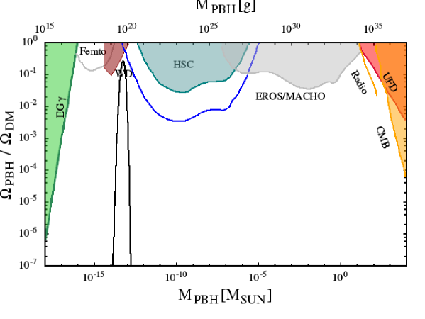
Figure 6: The fractional abundance of PBH for the first set of parameters in Table 2 (black line). Details on the various excluded regions due to observation data given in [56, 57, 58, 59, 60, 61, 62, 63, 64, 65, 66, 67, 68].

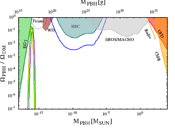
Figure 7: The fractional abundance of PBH, such as Fig. 6, for the last three sets of parameters in Table 2.

One should notice that the calculated PBH abundance is sensitive to the value of $\delta_{c}$. This value depends on the profile of the collapsing overdensities. Recent studies, assuming radiation domination, suggest that $\delta_{c}\approx 0.4-0.5$ [69, 70, 71, 72, 73, 74, 75, 76]. The same result is supported, by analytical calculations [74, 75] . Furthermore, one can notice by Eqs. (33) and(35) that the PBH abundance depends also on the value of the the power spectrum peak, since $\sigma$ is in the denominator in the exponential. This is an additional justification for employing the precise numerical solution of the M-S equation, instead of the slow-roll approximation.

Using this method, we are able to produce a significant abundance of PBH, modifying accordingly the Kähler potential, through the $b$ parameter. We summarize our results in Table 3, where we have used $\delta_{c}=0.45$. The sets of parameters in this table correspond to those in Table 2. We must stress that the amount of the fine-tuning in the parameter $b$, is related to the central value for the $\delta_{c}$ we have used. For example, using $\delta_{c}=0.5$, the values of $b$ as appear in Table 1 are less tuned in the last two digits. This means that allowing a slight variation on $\delta_{c}$, we can somewhat reduce the fine-tuning on $b$.

We plot the fractional abundance for the first set of parameters of Table 1 (Fig. 6). The observational data depicted in Figs. 6 and 7 are adapted by[9] with the bounds by refs[56, 57, 58, 59, 60, 61, 62, 63, 64, 65, 66, 67, 68]. Specifically, these bounds are from extragalactic gamma ray from PBH evaporation ($EG\gamma$) [56], femtolensing of gamma ray burst (Femto) [57], white dwarfs explosion (WD) [58], microlensing for Subaru (HSC) with dashed line shows the uncertain constraint of HSC and Eros/Macho [59, 60], dynamical heating of ultra faint dwarf (UFD) [61], CMB measurements [65] and radio observation [67]. Taking into account these bounds, in Fig. 6 we superimpose our results for the PBH abundance using the parameters of the first set in Table 3. This prediction is marked by a black solid line reaching values for $\Omega_{PBH}/\Omega_{DM}$ up to $0.2$, between the microlensing for Subaru and the white dwarfs explosion excluded regions.

Using the last three parameter sets in Table 1, we superimpose our results in Fig. 7. Purple line corresponds to $\lambda/\mu=0.33327$, orange to $0.33330$ and green to $1/3$. We notice that, although these three different parameter sets yield quite distinctive cosmological predictions, as can be seen in Fig. 3, by appropriate choice of the initial value for the field $\phi$ (see Table 2), we can achieve almost similar fractional abundance for all cases, as in Fig. 7. Finally, our results are consistent with the constraints calculated in ref. [77].

4 Conclusions

In this paper, we study a model based on a no-scale supergravity with $SU(2,1)/SU(2)\times U(1)$ symmetry [45], with a deformed Kähler potential by introducing a simple exponential term, using practically one extra parameter. The perturbation due to this modification induces an inflection point to the effective scalar potential. As expected, this potential, in the absence of the modification yields the usual Starobinsky-like potential. The superpotential we employ is the well-known Wess-Zumino superpotential. The induced inflection point can be expounded as a peak in the CMB power spectrum. Interestingly enough, using this mechanism we satisfy all the Planck cosmological constraints for inflation and we were able to achieve ample PBH production, that can explain up to 20%–25% of the DM of the Universe.

Moreover, we studied the stability of the potential along the inflationary directions, checking all the parameter sets presented in this work. Afterwards in the context of the slow-roll approximation, we use the single field inflation method and we evaluate the evolution of the field and the slow-roll parameters. We highlight that the slow-roll approximation fails to provide the precise power spectrum, therefore the use of the M-S equation is imperative. Eventually, using the numerical result from the M-S solution, we calculate the power spectrum and the fractional abundance of PBH.

We have scanned the parameters entering in the modified Kähler potential and we have presented results for various sets of them. Interestingly, we have found that potentials with values for the ratio $\lambda/\mu>1/3$, which are excluded by CMB constraints in the context of the original Wess-Zumino model, now become compatible with the latest Planck data. In parallel, these values of the parameters are compatible to significant amount of PBH.

Unfortunately, as all the inflation models that use the inflection point mechanism in order to produce PBH, our model requires fine-tuning of the parameters entering by the modification of the Kähler potential. Although, the numerical analysis reveals that this fine-tuning can be compensated in part, by the appropriate choice of the parameter $\delta_{c}$ that affects the calculation of the PBH abundance, a more detailed quantitative analysis on this aspect can be performed. Moreover, exploring inflationary models that are not using the inflection point mechanism in order to produce PBH, will alleviate the necessary fine-tuning. Both directions require detailed analysis, since the PBH is an interesting alternative to the standard DM models.

References

- [1] B. Abbott et al. [LIGO Scientific and Virgo], Phys. Rev. Lett. 116 (2016) no.6, 061102 doi:10.1103/PhysRevLett.116.061102 [arXiv:1602.03837 [gr-qc]].
- [2] B. P. Abbott et al. [LIGO Scientific and Virgo], Phys. Rev. Lett. 116 (2016) no.24, 241103 doi:10.1103/PhysRevLett.116.241103 [arXiv:1606.04855 [gr-qc]].
- [3] B. P. Abbott et al. [LIGO Scientific and VIRGO], Phys. Rev. Lett. 118 (2017) no.22, 221101 doi:10.1103/PhysRevLett.118.221101 [arXiv:1706.01812 [gr-qc]].
- [4] B. P. Abbott et al. [LIGO Scientific and Virgo], Astrophys. J. 851 (2017) no.2, L35 doi:10.3847/2041-8213/aa9f0c [arXiv:1711.05578 [astro-ph.HE]].
- [5] B. Abbott et al. [LIGO Scientific and Virgo], Phys. Rev. Lett. 119 (2017) no.14, 141101 doi:10.1103/PhysRevLett.119.141101 [arXiv:1709.09660 [gr-qc]].
- [6] J. Garcia-Bellido, A. D. Linde and D. Wands, Phys. Rev. D 54 (1996), 6040-6058 doi:10.1103/PhysRevD.54.6040 [arXiv:astro-ph/9605094 [astro-ph]].
- [7] S. M. Leach and A. R. Liddle, Phys. Rev. D 63 (2001), 043508 doi:10.1103/PhysRevD.63.043508 [arXiv:astro-ph/0010082 [astro-ph]].
- [8] A. M. Green and B. J. Kavanagh, [arXiv:2007.10722 [astro-ph.CO]].
- [9] G. Ballesteros and M. Taoso, Phys. Rev. D 97 (2018) no.2, 023501 doi:10.1103/PhysRevD.97.023501 [arXiv:1709.05565 [hep-ph]].
- [10] O. Özsoy, S. Parameswaran, G. Tasinato and I. Zavala, JCAP 07 (2018), 005 doi:10.1088/1475-7516/2018/07/005 [arXiv:1803.07626 [hep-th]].
- [11] M. Biagetti, G. Franciolini, A. Kehagias and A. Riotto, JCAP 07 (2018), 032 doi:10.1088/1475-7516/2018/07/032 [arXiv:1804.07124 [astro-ph.CO]].
- [12] G. Franciolini, A. Kehagias, S. Matarrese and A. Riotto, JCAP 03 (2018), 016 doi:10.1088/1475-7516/2018/03/016 [arXiv:1801.09415 [astro-ph.CO]].
- [13] T.J. Gao and Z.K. Guo, Phys. Rev. D 98 (2018) no.6, 063526 doi:10.1103/PhysRevD.98.063526 [arXiv:1806.09320 [hep-ph]].
- [14] M. Cicoli, V. A. Diaz and F. G. Pedro, JCAP 06 (2018), 034 doi:10.1088/1475-7516/2018/06/034 [arXiv:1803.02837 [hep-th]].
- [15] I. Dalianis, A. Kehagias and G. Tringas, JCAP 01 (2019), 037 doi:10.1088/1475-7516/2019/01/037 [arXiv:1805.09483 [astro-ph.CO]].
- [16] J. Garcia-Bellido and E. Ruiz Morales, Phys. Dark Univ. 18 (2017), 47-54 doi:10.1016/j.dark.2017.09.007 [arXiv:1702.03901 [astro-ph.CO]].
- [17] J. M. Ezquiaga, J. Garcia-Bellido and E. Ruiz Morales, Phys. Lett. B 776 (2018), 345-349 doi:10.1016/j.physletb.2017.11.039 [arXiv:1705.04861 [astro-ph.CO]].
- [18] H. Di and Y. Gong, JCAP 07 (2018), 007 doi:10.1088/1475-7516/2018/07/007 [arXiv:1707.09578 [astro-ph.CO]].
- [19] M. P. Hertzberg and M. Yamada, Phys. Rev. D 97 (2018) no.8, 083509 doi:10.1103/PhysRevD.97.083509 [arXiv:1712.09750 [astro-ph.CO]].
- [20] J.R. Espinosa, D. Racco and A. Riotto, Phys. Rev. Lett. 120 (2018) no.12, 121301 doi:10.1103/PhysRevLett.120.121301 [arXiv:1710.11196 [hep-ph]].
- [21] S. Clesse and J. Garcia-Bellido, Phys. Rev. D 92 (2015) no.2, 023524 doi:10.1103/PhysRevD.92.023524 [arXiv:1501.07565 [astro-ph.CO]].
- [22] C. Germani and T. Prokopec, Phys. Dark Univ. 18 (2017), 6-10 doi:10.1016/j.dark.2017.09.001 [arXiv:1706.04226 [astro-ph.CO]].
- [23] K. Inomata, M. Kawasaki, K. Mukaida, Y. Tada and T. T. Yanagida, Phys. Rev. D 96 (2017) no.4, 043504 doi:10.1103/PhysRevD.96.043504 [arXiv:1701.02544 [astro-ph.CO]].
- [24] H. Motohashi and W. Hu, Phys. Rev. D 96 (2017) no.6, 063503 doi:10.1103/PhysRevD.96.063503 [arXiv:1706.06784 [astro-ph.CO]].
- [25] K. Kannike, L. Marzola, M. Raidal and H. Veermäe, JCAP 09 (2017), 020 doi:10.1088/1475-7516/2017/09/020 [arXiv:1705.06225 [astro-ph.CO]].
- [26] K. Inomata, M. Kawasaki, K. Mukaida and T. T. Yanagida, Phys. Rev. D 97 (2018) no.4, 043514 doi:10.1103/PhysRevD.97.043514 [arXiv:1711.06129 [astro-ph.CO]].
- [27] M. Kawasaki, A. Kusenko, Y. Tada and T. T. Yanagida, Phys. Rev. D 94 (2016) no.8, 083523 doi:10.1103/PhysRevD.94.083523 [arXiv:1606.07631 [astro-ph.CO]].
- [28] B. Carr, F. Kuhnel and M. Sandstad, Phys. Rev. D 94 (2016) no.8, 083504 doi:10.1103/PhysRevD.94.083504 [arXiv:1607.06077 [astro-ph.CO]].
- [29] S. Cheng, W. Lee and K. Ng, JCAP 07 (2018), 001 doi:10.1088/1475-7516/2018/07/001 [arXiv:1801.09050 [astro-ph.CO]].
- [30] R. Mahbub, Phys. Rev. D 101 (2020) no.2, 023533 doi:10.1103/PhysRevD.101.023533 [arXiv:1910.10602 [astro-ph.CO]].
- [31] S. S. Mishra and V. Sahni, JCAP 04 (2020), 007 doi:10.1088/1475-7516/2020/04/007 [arXiv:1911.00057 [gr-qc]].
- [32] G. Ballesteros, J. Rey and F. Rompineve, JCAP 06 (2020), 014 doi:10.1088/1475-7516/2020/06/014 [arXiv:1912.01638 [astro-ph.CO]].
- [33] M. Braglia, D. K. Hazra, F. Finelli, G. F. Smoot, L. Sriramkumar and A. A. Starobinsky, [arXiv:2005.02895 [astro-ph.CO]].
- [34] R. G. Cai, Z. K. Guo, J. Liu, L. Liu and X. Y. Yang, JCAP 06 (2020), 013 doi:10.1088/1475-7516/2020/06/013 [arXiv:1912.10437 [astro-ph.CO]].
- [35] Y. Aldabergenov, A. Addazi and S. V. Ketov, [arXiv:2006.16641 [hep-th]].
- [36] S. V. Ketov and M. Y. Khlopov, Symmetry 11 (2019) no.4, 511 doi:10.3390/sym11040511
- [37] V. F. Mukhanov, Sov. Phys. JETP 67 (1988), 1297-1302
- [38] M. Sasaki, Prog. Theor. Phys. 76 (1986), 1036 doi:10.1143/PTP.76.1036
- [39] J. R. Ellis, A. Lahanas, D. V. Nanopoulos and K. Tamvakis, Phys. Lett. B 134 (1984), 429 doi:10.1016/0370-2693(84)91378-9
- [40] E. Cremmer, S. Ferrara, C. Kounnas and D. V. Nanopoulos, Phys. Lett. B 133 (1983), 61 doi:10.1016/0370-2693(83)90106-5
- [41] J. R. Ellis, C. Kounnas and D. V. Nanopoulos, Nucl. Phys. B 241 (1984), 406-428 doi:10.1016/0550-3213(84)90054-3
- [42] J. R. Ellis, C. Kounnas and D. V. Nanopoulos, Nucl. Phys. B 247 (1984), 373-395 doi:10.1016/0550-3213(84)90555-8
- [43] A. Lahanas and D. V. Nanopoulos, Phys. Rept. 145 (1987), 1 doi:10.1016/0370-1573(87)90034-2
- [44] E. Witten, Phys. Lett. B 155 (1985), 151 doi:10.1016/0370-2693(85)90976-1
- [45] J. Ellis, D. V. Nanopoulos and K. A. Olive, Phys. Rev. Lett. 111 (2013), 111301 doi:10.1103/PhysRevLett.111.111301 [arXiv:1305.1247 [hep-th]].
- [46] Y. Akrami et al. [Planck], [arXiv:1807.06211 [astro-ph.CO]].
- [47] P. Ade et al. [Planck], Astron. Astrophys. 594 (2016), A20 doi:10.1051/0004-6361/201525898 [arXiv:1502.02114 [astro-ph.CO]].
- [48] N. Aghanim et al. [Planck], [arXiv:1807.06209 [astro-ph.CO]].
- [49] J. Ellis, D. V. Nanopoulos and K. A. Olive, JCAP 10 (2013), 009 doi:10.1088/1475-7516/2013/10/009 [arXiv:1307.3537 [hep-th]].
- [50] S. Cecotti, Phys. Lett. B 190 (1987), 86-92 doi:10.1016/0370-2693(87)90844-6
- [51] J. Ellis, D. V. Nanopoulos, K. A. Olive and S. Verner, JCAP 09 (2019), 040 doi:10.1088/1475-7516/2019/09/040 [arXiv:1906.10176 [hep-th]].
- [52] J. Ellis, B. Nagaraj, D. V. Nanopoulos and K. A. Olive, JHEP 11 (2018), 110 doi:10.1007/JHEP11(2018)110 [arXiv:1809.10114 [hep-th]].
- [53] J. A. Adams, B. Cresswell and R. Easther, Phys. Rev. D 64 (2001), 123514 doi:10.1103/PhysRevD.64.123514 [arXiv:astro-ph/0102236 [astro-ph]].
- [54] W. H. Press and P. Schechter, Astrophys. J. 187 (1974), 425-438 doi:10.1086/152650
- [55] B. J. Carr, Astrophys. J. 201 (1975), 1-19 doi:10.1086/153853
- [56] B.J. Carr, K. Kohri, Y. Sendouda and J. Yokoyama, Phys. Rev. D 81 (2010), 104019 doi:10.1103/PhysRevD.81.104019 [arXiv:0912.5297 [astro-ph.CO]].
- [57] A. Barnacka, J.F. Glicenstein and R. Moderski, Phys. Rev. D 86 (2012), 043001 doi:10.1103/PhysRevD.86.043001 [arXiv:1204.2056 [astro-ph.CO]].
- [58] P. W. Graham, S. Rajendran and J. Varela, Phys. Rev. D 92 (2015) no.6, 063007 doi:10.1103/PhysRevD.92.063007 [arXiv:1505.04444 [hep-ph]].
- [59] F. Capela, M. Pshirkov and P. Tinyakov, Phys. Rev. D 87 (2013) no.12, 123524 doi:10.1103/PhysRevD.87.123524 [arXiv:1301.4984 [astro-ph.CO]].
- [60] H. Niikura, M. Takada, N. Yasuda, R. H. Lupton, T. Sumi, S. More, T. Kurita, S. Sugiyama, A. More, M. Oguri and M. Chiba, Nat. Astron. 3 (2019) no.6, 524-534 doi:10.1038/s41550-019-0723-1 [arXiv:1701.02151 [astro-ph.CO]].
- [61] P. Tisserand et al. [EROS-2], Astron. Astrophys. 469 (2007), 387-404 doi:10.1051/0004-6361:20066017 [arXiv:astro-ph/0607207 [astro-ph]].
- [62] M. A. Monroy-Rodríguez and C. Allen, Astrophys. J. 790 (2014) no.2, 159 doi:10.1088/0004-637X/790/2/159 [arXiv:1406.5169 [astro-ph.GA]].
- [63] T. D. Brandt, Astrophys. J. 824 (2016) no.2, L31 doi:10.3847/2041-8205/824/2/L31 [arXiv:1605.03665 [astro-ph.GA]].
- [64] S. M. Koushiappas and A. Loeb, Phys. Rev. Lett. 119 (2017) no.4, 041102 doi:10.1103/PhysRevLett.119.041102 [arXiv:1704.01668 [astro-ph.GA]].
- [65] Y. Ali-Haimoud and M. Kamionkowski, Phys. Rev. D 95 (2017) no.4, 043534 doi:10.1103/PhysRevD.95.043534 [arXiv:1612.05644 [astro-ph.CO]].
- [66] V. Poulin, P. D. Serpico, F. Calore, S. Clesse and K. Kohri, Phys. Rev. D 96 (2017) no.8, 083524 doi:10.1103/PhysRevD.96.083524 [arXiv:1707.04206 [astro-ph.CO]].
- [67] D. Gaggero, G. Bertone, F. Calore, R. M. T. Connors, M. Lovell, S. Markoff and E. Storm, Phys. Rev. Lett. 118 (2017) no.24, 241101 doi:10.1103/PhysRevLett.118.241101 [arXiv:1612.00457 [astro-ph.HE]].
- [68] Y. Inoue and A. Kusenko, JCAP 10 (2017), 034 doi:10.1088/1475-7516/2017/10/034 [arXiv:1705.00791 [astro-ph.CO]].
- [69] T. Harada, C.M. Yoo and K. Kohri, Phys. Rev. D 88 (2013) no.8, 084051 doi:10.1103/PhysRevD.88.084051 [arXiv:1309.4201 [astro-ph.CO]].
- [70] I. Musco and J. C. Miller, Class. Quant. Grav. 30 (2013), 145009 doi:10.1088/0264-9381/30/14/145009 [arXiv:1201.2379 [gr-qc]].
- [71] J. R. Chisholm, Phys. Rev. D 74 (2006), 043512 doi:10.1103/PhysRevD.74.043512 [arXiv:astro-ph/0604174 [astro-ph]].
- [72] I. Musco, J. C. Miller and A. G. Polnarev, Class. Quant. Grav. 26 (2009), 235001 doi:10.1088/0264-9381/26/23/235001 [arXiv:0811.1452 [gr-qc]].
- [73] I. Musco, J. C. Miller and L. Rezzolla, Class. Quant. Grav. 22 (2005), 1405-1424 doi:10.1088/0264-9381/22/7/013 [arXiv:gr-qc/0412063 [gr-qc]].
- [74] A. Escriva, C. Germani and R. K. Sheth, Phys. Rev. D 101 (2020) no.4, 044022 doi:10.1103/PhysRevD.101.044022 [arXiv:1907.13311 [gr-qc]].
- [75] A. Escrivà, C. Germani and R. K. Sheth, [arXiv:2007.05564 [gr-qc]].
- [76] C. Germani and I. Musco, Phys. Rev. Lett. 122 (2019) no.14, 141302 doi:10.1103/PhysRevLett.122.141302 [arXiv:1805.04087 [astro-ph.CO]].
- [77] R. Laha, J. B. Munoz and T. R. Slatyer, Phys. Rev. D 101 (2020) no.12, 123514 doi:10.1103/PhysRevD.101.123514 [arXiv:2004.00627 [astro-ph.CO]].