Learning from a Complementary-label Source Domain: Theory and Algorithms
Abstract
In unsupervised domain adaptation (UDA), a classifier for the target domain is trained with massive true-label data from the source domain and unlabeled data from the target domain. However, collecting fully-true-label data in the source domain is high-cost and sometimes impossible. Compared to the true labels, a complementary label specifies a class that a pattern does not belong to, hence collecting complementary labels would be less laborious than collecting true labels. Thus, in this paper, we propose a novel setting that the source domain is composed of complementary-label data, and a theoretical bound for it is first proved. We consider two cases of this setting, one is that the source domain only contains complementary-label data (completely complementary unsupervised domain adaptation, CC-UDA), and the other is that the source domain has plenty of complementary-label data and a small amount of true-label data (partly complementary unsupervised domain adaptation, PC-UDA). To this end, a complementary label adversarial network (CLARINET) is proposed to solve CC-UDA and PC-UDA problems. CLARINET maintains two deep networks simultaneously, where one focuses on classifying complementary-label source data and the other takes care of source-to-target distributional adaptation. Experiments show that CLARINET significantly outperforms a series of competent baselines on handwritten-digits-recognition and objects-recognition tasks.
Index Terms:
Transfer Learning; Machine Learning; Deep Learning; Complementary LabelsI Introduction
Domain Adaptation (DA) aims to train a target-domain classifier with data in source and target domains [1, 2, 3]. Based on the availability of data in the target domain (e.g., fully-labeled, partially-labeled and unlabeled), DA is divided into three categories: supervised DA [4, 5, 6], semi-supervised DA [7, 8, 9] and unsupervised DA (UDA) [10, 11, 12]. In practical applications, UDA is more challenging and promising than the other two as the labeled target domain data are not needed [13, 14, 15].
UDA methods train a target-domain classifier with massive true-label data from the source domain (true-label source data) and unlabeled data from the target domain (unlabeled target data). Existing works in the literature can be roughly categorised into the following three groups: integral-probability-metrics based UDA [16, 17]; adversarial-training based UDA [18, 19]; and causality-based UDA [20, 21]. Since adversarial-training based UDA methods extract better domain-invariant representations via deep networks, they usually have good target-domain accuracy [22].
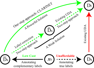
However, the success of UDA still highly relies on the scale of true-label source data (black dash line in Figure 1). Namely, the target-domain accuracy of a UDA method (e.g., CDAN) decays when the scale of true-label source data decreases and we prove this phenomenon in the experiment section. Hence, massive true-label source data are inevitably required by UDA methods, which is very expensive and even prohibitive.
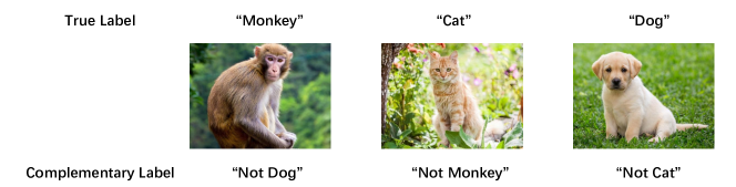
While determining the correct label from many candidates is laborious, choosing one of the incorrect labels (i.e., complementary labels), e.g. labeling a cat as “Not Monkey” (as shown in Figure 2), would be much easier and quicker, thus less costly, especially when we have many candidates [23]. For example, suppose that we need to annotate the labels of a bunch of animal images from candidates. One strategy is to ask crowd-workers to choose the true labels from candidates, while the other is to judge the correctness of a label randomly given by the system from the candidates. Apparently, the cost of the second strategy is much lower [24, 25].
This brings us a novel setting, complementary-label based UDA, which aims to transfer knowledge from complementary-label source data to unlabeled target data (Figure 1). Compared to ordinary UDA, we can greatly save the labeling cost by annotating complementary labels in the source domain rather than annotating true labels [23, 26]. Please note, existing UDA methods cannot handle complementary-label based UDA, as they require fully-true-label source data [11, 12] or at least true-label source data [27, 28].
In our previous conference paper [29], we consider using completely complementary-label data in the source domain while actually we could also get a small amount of true labels when collecting complementary labels [23]. Therefore, the previous work was flawed as it did not make good use of the existing true-label data. Furthermore, experiments were conducted only on some digit datasets and a thorough learning bound was not provided. Aiming at these defects, in this work, we consider a generalized and completed version of the complementary-label based UDA problem setting.
A straightforward but weak solution to complementary-label based UDA is a two-step approach, which sequentially combines complementary-label learning methods and existing UDA methods (green dash line in Figure 1)111We implement this two-step approach and take it as a baseline.. Complementary-label learning methods are used to assign pseudo labels for complementary-label source data. Then, we can train a target-domain classifier with pseudo-label source data and unlabeled target data using existing UDA methods. Nevertheless, pseudo-label source data contain noise, which may cause poor domain-adaptation performance of this two-step approach [27].
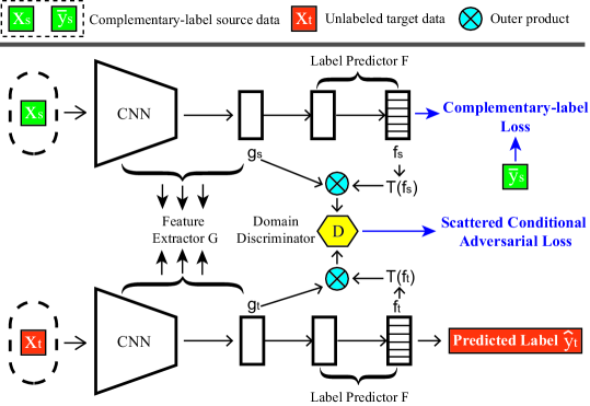
Therefore, we propose a powerful one-step solution, complementary label adversarial network (CLARINET). It maintains two deep networks trained by adversarial way simultaneously, where one can accurately classify complementary-label source data, and the other can discriminate source and target domains. Since Long et. al. [19] and Song et. al. [30] have shown that the multimodal structures of distributions can only be captured sufficiently by the cross-covariance dependency between the features and classes (i.e., true labels), we set the input of domain discriminator as the outer product of feature representation (e.g., in Figure 3) and mapped classifier prediction (e.g., in Figure 3).
Due to the nature of complementary-label classification, the predicted probability of each class (i.e., each element of , Figure 3) is relatively close. According to [30], this kind of predicted probabilities could not provide sufficient information to capture the multimodal structure of distributions. To fix it, we add a sharpening function to make the predicted probabilities more scattered (i.e., , Figure 3) than previous ones (i.e., , Figure 3). By doing so, the mapped classifier predictions can better indicate their choice. In this way, we can take full advantage of classifier predictions and effectively align distributions of two domains. Our ablation study (see Table III) verifies that the sharpening function indeed helps improve the target-domain accuracy.
We conduct experiments on complementary-label based UDA tasks and compare CLARINET with a series of competent baselines. Empirical results demonstrated that CLARINET effectively transfers knowledge from complementary-label source data to unlabeled target data and is superior to all baselines. We also show that the target-domain accuracy of CLARINET will increase if a small amount of true-label source data are available. To make up for the defects of previous conference paper [29], the main contributions of this paper are summarized as follows.
-
1)
We present a generalized version of the complementary-label based UDA. This paper considers two cases of complementary-label based UDA, one is that the source domain only contains complementary-label data (completely complementary unsupervised domain adaptation, CC-UDA), and the other is that the source domain also contains a small amount of true-label data (partly complementary unsupervised domain adaptation, PC-UDA).
-
2)
We provide a thorough theoretical analysis of the expected target-domain risk of our approach, presenting a learning bound of complementary-label based UDA.
-
3)
Apart from the handwritten digit datasets, we also conduct experiments on more complex image datasets, proving the applicability of complementary-label based UDA.
This paper is organized as follows. Section II reviews the works related to domain adaptation, complementary-label learning, and low-cost unsupervised domain adaptation. Section III introduces the problem setting and prove a learning bound of this problem. Section IV introduces a straightforward but weak two-step approach to complementary-label based UDA. The proposed powerful one-step solution is shown in Section V. Experimental results and analyses are provided in Section VI. Finally, Section VII concludes this paper.
II Related Works
In this section, we discuss previous works that are most related to our work, and highlight our differences from them. We mainly review some related works about domain adaptation, complementary-label learning and low-cost unsupervised domain adaptation.
II-A Domain Adaptation
Domain adaptation generalizes a learner across different domains by matching the distributions of source and target domains. It has wide application in computer vision [31, 32, 33] and natural language processing [34, 35], etc. Previous domain adaptation methods in the shallow regime either try to bridge the source and target by learning invariant feature representations or estimating instance importances using labeled source data and unlabeled target data [36, 37]. Later, it is confirmed that deep learning methods formed by the composition of multiple non-linear transformations yield abstract and ultimately useful representations [38]. Besides, the learned deep representations to some extent are general and are transferable to similar tasks [39]. Hence, deep neural networks have been explored for domain adaptation.
Concurrently, multiple methods of matching the feature distributions in the source and the target domains have been proposed for unsupervised domain adaptation. The first category learns domain invariant features by minimizing a distance between distributions, such as Maximum Mean Discrepancy (MMD) [40]. In DAN [16], Long et.al. minimize the marginal distributions of two domains by multi-kernel MMD (MK-MMD) metric. An alternative way of learning domain invariant features in UDA is inspired by the Generative Adversarial Networks (GANs). By confusing a domain classifier (or discriminator), the deep networks can explore non-discriminative representations. The adversarial-training based UDA methods always try to play a two-player minimax game. DANN [41] employs a gradient reversal layer to realize the minimax optimation. In [19], Long et.al. propose conditional domain adversarial network (CDAN) which conditions the models on discriminative information conveyed in the classifier predictions. Some works study the UDA problem from a causal point of view where they consider the label is the cause for feature representation . In [20], Gong et. al. aim to extract conditional transferable components whose conditional distribution is invariant after proper location-scale (LS) transformations.
However, the aforementioned methods all based on the true-label source domain data, which require high labeling costs. In our work, we propose a new setting which use complementary-label source data instead of true-label source data, which significantly save the labeling cost.
II-B Complementary-label Learning
Complementary-label learning (shown in Figure 2) is one type of weak supervision learning approaches, which is first proposed by Ishida et. al. [23]. They gave theoretical analysis with a statistical consistency guarantee to show classification risk can be recovered only from complementary-label data. Nevertheless, they require the complementary label must be chosen in an unbiased way and allow only one-versus-all and pairwise comparison multi-class loss functions with certain non-convex binary losses. Namely softmax cross-entropy loss, which is the most popular loss in deep learning, could not be used to solve the problem.
Later, Yu et. al. [26] extend the problem setting to where complementary label could be chosen in biased way with the assumption that a small set of easily distinguishable true-label data are available in practice. In their point of view, due to humans are biased toward their own experience, it is unrealistic to guarantee the complementary label is chosen in an unbiased way. For example, if an annotator is more familiar with one class than with another, she is more likely to employ the more familiar one as a complementary label. They solve the problem by employing the forward loss correction technique to adjust the learning objective, but limiting the loss function to softmax cross-entropy loss. They theoretically ensure that the classifier learned with complementary labels converges to the optimal one learned with true labels.
Recently, Ishida et. al. propose a new unbiased risk estimator [24] under the unbiased label chosen assumption. They make any loss functions available for use and have no implicit assumptions on the classifier, namely the estimator could be used for arbitrary models and losses, including softmax cross-entropy loss. They further investigate correction schemes to make complementary label learning practical and demonstrate the performance. Thus in our paper, we take advantage of this estimator for the source domain classification and generalize it to the unsupervised domain adaptation field.
II-C Low-cost Unsupervised Domain Adaptation
Unsupervised domain adaptation with low cost source data has recently attracted attention. For instance, in [27], Liu et. al. consider the situation that the labeled data in the source domain come from amateur annotators or the Internet [42, 43]. As in the wild, acquiring a large amount of perfectly clean labeled data in the source domain is high-cost and sometimes impossible. They name the problem as wildy unsupervised domain adaptation (abbreviated as WUDA), which aims to transfer knowledge from noisy labeled data in the source domain to unlabeled target data. They show that WUDA ruins all UDA methods if taking no care of label noise in the source domain and propose a Butterfly framework, a powerful and efficient solution to WUDA.
Long et. al. consider the weakly-supervised domain adaptation, where the source domain with noises in labels, features, or both could be tolerated [28]. Label noise refers to incorrect labels of images due to errors in manual annotation, and feature noise refers to low-quality pixels of images, which may come from blur, overlap, occlusion, or corruption etc. They present a Transferable Curriculum Learning (TCL) approach, extending from curriculum learning and adversarial learning. The TCL model aims to be robust to both sample noises and distribution shift by employing a curriculum which could tell whether a sample is easy and transferable.
In [29], we consider another way to save the labeling cost by using completely complementary-label data in the source domain and prove that distributional adaptation can be effectively realized from complementary-label source data to unlabeled target data. In this paper, we consider two cases of using complementary-label data in the source domain and prove that we could use a small amount of true-label data to improve the transfer result. Besides, as shown in [23], we can obtain true-label data and complementary-label data simultaneously so that getting a small amount of true-label data is guaranteed to be low-cost. Furthermore, we provide an analysis of the expected target-domain risk of our approach. In the following sections, we will introduce the complementary-label based UDA and explain how to address such tasks.
III Complementary-label Based Unsupervised Domain Adaptation
In this section, we propose a novel problem setting, complementary-label based UDA, and prove a learning bound for it. Then, we show how it brings benefits to domain adaptation field.
III-A Problem Setting
In complementary-label based UDA, we aim to realize distributional adaptation from complementary-label source data to unlabeled target data. We first consider the situation that there are only complementary-label data in the source domain, namely completely complementary unsupervised domain adaptation (CC-UDA). Let be a feature (input) space and be a label (output) space, where is the one-hot vector for label . A domain is defined as follows.
Definition 1 (Domains for CC-UDA).
Given random variables , , the source and target domains are joint distributions and , where the joint distributions and for all .
Then, we propose CC-UDA problem as follows.
Problem 1 (CC-UDA).
Given independent and identically distributed (i.i.d.) labeled samples drawn from the source domain and i.i.d. unlabeled samples drawn from the target marginal distribution , the aim of CC-UDA is to train a classifier with and such that can accurately classify target data drawn from .
It is clear that it is impossible to design a suitable learning procedure without any assumptions on . In this paper, we use the assumption for unbiased complementary learning proposed by [23, 24]:
| (1) |
for all and . This unbiased assumption indicates that the selection of complementary labels for samples is with equal probability.
Ishida et. al. [23] proposed an efficient way to collect labels through crowdsourcing: we choose one of the classes randomly and ask crowdworkers whether a pattern belongs to the chosen class or not. Then the chosen class is treated as true label if the answer is yes; otherwise, the chosen class is regarded as complementary label. Such a yes/no question is much easier and quicker than selecting the correct class from the list of all candidate classes. In addition, we could guarantee that the complementary-label data gotten through this way are under unbiased assumption in Eq. (1).
As we can obtain true-label data and complementary-label data simultaneously, we also consider the problem that the source domain contains a few true-label data. We name this problem as partly complementary-label unsupervised domain adaptation (PC-UDA).
Problem 2 (PC-UDA).
Given i.i.d labeled samples drawn from the domain , drawn from the domain , and i.i.d unlabeled samples drawn from the target marginal distribution , the aim is to find a target classifier such that classifies target samples into the correct classes.
It is actually a more common situation to have a small number of true-label data. If we leverage both kind of labeled data properly, we could obtain a more accurate classifier. Ishida et. al. [23] have demonstrated that the usefulness of combining true-label and complementary-label data in classification problem. We will further show that in unsupervised domain adaptation field, we could also use both true-label and complementary-label source data to realize knowledge transfer and utilize the true-label data to improve the result.
III-B Learning Bound of complementary-label based UDA
A learning bound of complementary-label based UDA is presented in this subsection. We could prove that we can limit the risk in the target domain. Practitioner may safely skip it.
If given a feature transformation:
| (2) |
then the induced distributions related to and are
| (3) |
Following the notations in [44], consider a multi-class classification task with a hypothesis space of the classifiers
| (4) |
Let
| (5) |
be the loss function. For convenience, we also require satisfying the following conditions in theoretical part:
1. is symmetric and satisfies triangle inequality;
2. iff ;
3. if and are one-hot vectors.
We can check many losses satisfying the above conditions such as - loss and loss . The complementary risk for with respect to over is
The risks for the decision function with respect to loss over implicit distribution are:
In this paper, we propose a tighter distance named tensor discrepancy distance. The tensor discrepancy distance can future math the pseudo conditional distributions.
We consider the following tensor mapping:
| (6) |
Then we induce two importance distributions:
| (7) |
Using , we reconstruct a new hypothetical set:
| (8) |
where . Then the distance between and is:
| (9) |
where is the sign function.
It is easy to prove that under the conditions (1)-(3) for loss and for any , we have
| (10) |
where is the distribution discrepancy defined in [45, 46]. Then, we introduce our main theorem as follows.
Theorem 1.
Given a loss function satisfying conditions 1-3 and a hypothesis , then under unbiased assumption, for any , we have
where , are source and target marginal distributions, .
Proof.
Firstly, we prove that . To prove it, we investigate the connection between and under unbiased assumption in Eq. (1). Given matrix whose diagonal elements are and other elements are , we represent the unbiased assumption by
| (11) |
where and . Note that has inverse matrix whose diagonal elements are and other elements are . Thus, we have that
| (12) |
According to Eq. (12), we have , which implies that
| (13) |
Hence, . The empirical form of Eq. (13) is known as complementary-label loss (see Eq. (20)).
Next we will prove that
As if it is true, combined with , we could easily prove the theorem. It is clearly that
| (14) |
where is any function from . According to conditions 1-3, we have that
III-C Benefits to DA Field
Collecting true-label data is always expensive in the real world. Thus, learning from less expensive data [47, 48, 49, 50] has been extensively studied in machine learning field, including label-noise leaning [51, 52, 53], pairwise/triple-wise constraints learning [54, 55, 56], positive-unlabeled learning [57, 58, 59], complementary-label learning [23, 24, 26] and so on. Among all these research directions, obtaining complementary labels is a cost-effective option. As described in the previous works mentioned above, compared with choosing the true class out of many candidate classes precisely, collecting complementary labels is obviously much easier and less costly. In addition, a classifier trained with complementary-label data is equivalent to a classifier trained with true-label data as shown in [24].
Actually in the field of domain adaptation, the high cost of true-label data is also an important issue. At present, the success of DA still highly relies on the scale of true-label source data, which is a critical bottleneck. Under low cost limitation, it is unrealistic to obtain enough true-label source data and thus cannot achieve a good distribution adaptation result. For the same cost, we can get multiple times more complementary-label data than the true-label data. In addition, the adaptation scenario is limited to some commonly used datasets, e.g. handwritten digit datasets, as they have sufficient true labels to support distributional adaptation. This fact makes it difficult to generalize domain adaptation to more real-world scenarios where it is needed. Thus if we can reduce the labeling cost in the source domain, for example, by using complementary-label data to replace true-label data (complementary-label based UDA), we can promote domain adaptation to more fields.
Due to existing UDA methods require at least true-label source data [28], they cannot handle complementary-label based UDA problem. To address the problem, we introduce a two-step approach, straightforward but weak solution, and then propose a powerful one-step solution, CLARINET.
Input: , .
Output: the target-domain classifier.
IV Two-step Approach
To solve the problem that existing UDA methods cannot be applied to complementary-label based UDA problems directly, a straightforward way is to apply a two-step strategy. Namely, we could sequentially combine complementary-label learning methods and existing UDA methods. Algorithm 1 presents how we realize two-step approach for CC-UDA tasks specifically. In two-step approach, we first use the complementary-label learning algorithm to train a classifier on the complementary-label source data (line 1). Then, we take advantage of the classifier to assign pseudo labels for source domain data (line 2). Finally, we train the target-domain classifier with pseudo-label source data and unlabeled target data using existing UDA methods (line 3). In this way, we can transfer knowledge from the newly formed pseudo-label source data to unlabeled target data. As for PC-UDA tasks, we could combine the pseudo-label source data gotten following the first two steps and existing true-label source data together to train the target-domain classifier.
Nevertheless, the pseudo-label source data contains noise as complementary-label learning algorithms cannot be trained to produce a completely accurate classifier. As the noise will bring poor domain-adaptation performance [27], the two-step approach is a suboptimal choice. To solve this problem, we consider implementing both complementary label learning and unsupervised domain adaptation in a network. In this way, the network will always try to classify source domain data accurately during the adaptation procedure. Besides, we consider using entropy condition to make the transfer process mainly based on the classification results with high confidence, which can largely eliminate the noise effect compared with the two-step approach. Therefore, we propose a powerful one-step solution to complementary-label based UDA, CLARINET.
V CLARINET: Powerful One-step Approach
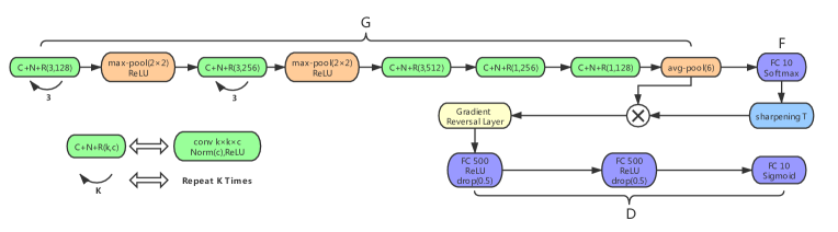
The proposed CLARINET (as shown in Figure 3) realizes distributional adaptation in an adversarial way, which mainly consists of feature extractor , label predictor and domain discriminator . By working adversarially to domain discriminator , feature extractor encourages domain-invariant features to emerge. Label predictor are trained to discriminate different classes based on such features.
In this section, we first introduce two losses used to train CLARINET, complementary-label loss and scattered conditional adversarial loss. Then the whole training procedure of CLARINET is presented. Finally, we show how to adjust CLARINET for PC-UDA tasks if a small amount of true-label source data are available.
V-A Loss Function in CLARINET
In this subsection, we introduce how to compute the two losses mentioned above in CLARINET after obtaining mini-batch from and from .
V-A1 Complementary-label Loss.
It is designed to reduce the source classification error based on complementary-label data (the first part in the bound). We first divided into disjoint subsets according to the complementary labels in ,
| (19) |
where if and . Then, following Eq. (13), the complementary-label loss on is
| (20) |
where can be any loss and we use the cross-entropy loss, is the proportion of the samples complementary-labeled . The total complementary-label loss on is as follows.
| (21) |
V-A2 Scattered Conditional Adversarial Loss.
It is designed to reduce distribution discrepancy distance between two domains (the third part in the bound). Adversarial domain adaptation methods [18, 61] is inspired by Generative Adversarial Networks (GANs) [62]. Normally, a domain discriminator is learned to distinguish the source domain and the target domain, while the label predictor learns transferable representations that are indistinguishable by the domain discriminator. Namely, the final classification decisions are made based on features that are both discriminative and invariant to the change of domains [18]. It is an efficient way to reduce distribution discrepancy distance between the marginal distributions.
However, when data distributions have complex multimodal structures, which is a real scenario due to the nature of multi-class classification, adapting only the feature representation is a challenge for adversarial networks. Namely, even the domain discriminator is confused, we could not confirm the two distributions are sufficiently similar [63].
According to [30], it is significant to capture multimodal structures of distributions using cross-covariance dependency between the features and classes (i.e., true labels). Since there are no true-label target data in UDA, CDAN adopts outer product of feature representations and classifier predictions (i.e., outputs of the softmax layer) as new features of two domains [19], which is inspired by Conditional Generative Adversarial Networks (CGANs) [64, 65]. The newly constructed features have shown great ability to discriminate source and target domains, since classifier predictions of true-label source data are dispersed, expressing the predicted goal clearly.
However, in the complementary-label classification mode, we observe that the predicted probability of each class (i.e., each element of in Figure 3) is relatively close. Namely, it is hard to find significant predictive preference from the classifier predictions. According to [30], this kind of predictions cannot provide sufficient information to capture the multimodal structure of distributions. To fix it, we add a sharpening function to scatter the predicted probability (the output of after Softmax function, could be or in Figure 3).
In [66], a common approach of adjusting the “temperature” of this categorical distribution is defined as follows,
| (22) |
As , the output of will approach a Dirac (“one-hot”) distribution [67].
Then to prioritize the discriminator on those easy-to-transfer examples, following [19], we measure the uncertainty of the prediction for sample by
| (23) |
The small result implies that is close to 0 or 1, which could be regarded as the prediction is with high confidence due to the existing of the final softmax layer [68].
Thus the scattered conditional adversarial loss is as follows,
| (24) |
where and are , is and is the feature part of .
Input: , .
Parameters: learning rate and , epoch , start epoch , iteration , class number , tradeoff , network parameter and .
Output: the neural network , namely the target domain classifier for .
V-B Training Procedure of CLARINET
Based on two losses proposed in Section V-A, in CLARINET, we try to solve the following optimization problem,
| (25) |
where tries to distinguish the samples from different domains by minimizing , while wants to maximize the to make domains indistinguishable. To solve the minimax optimization problem in Eq. (25), we add a gradient reversal layer [18] between the domain discriminator and the classifier, which multiplies the gradient by a negative constant (-) during the back-propagation. is a hyper-parameter between the two losses to tradeoff source risk and domain discrepancy.
The training procedures of CLARINET are shown in Algorithm 2. First, we initialize the whole network (line ) and shuffle the training set (line ). During each epoch, after minbatch and are fetched (line ), we divide the source mini-batch into using Eq. (19) (line ). Then, are used to calculate the complementary-label loss for each class (i.e., ) and the whole complementary-label loss (line ).
If , we calculate the gradient and update parameters of and using gradient descent (lines -). Otherwise, we sum negative elements in as (line ) and calculate the gradient with (line ). Then, we update parameters of and using gradient ascent (line ), which is suggested by [24]. When the number of epochs (i.e., ) is over , we start to update parameters of (line ). We calculate the scattered conditional adversarial loss (line ). Then, is minimized over (line ), but maximized over (line ) for adversarial training.
V-C CLARINET for PC-UDA Tasks
For PC-UDA tasks, we have both complementary-label data and true-label data in the source domain. In such cases, we want to leverage both kinds of labeled source data to help realize better adaptation results. The two loss functions mentioned in Section V-A are adjusted as follows.
After obtaining mini-batch from , we could calculate the classification loss based on true-label data by
| (26) |
where is cross-entropy loss, and . We could use a convex combination of classification risks derived from true-label data and complementary-label data to replace the oral complementary-label based only classification risk shown as following.
| (27) |
where depends on the cost of labeling the two kind of data.
The new scattered conditional adversarial loss for PC-UDA tasks is as follows.
| (28) |
where , and are , is , and is the feature part of and . The entire training procedures of CLARINET for PC-UDA are shown in Algorithm 3.
Input: , , .
Parameters: learning rate and , epoch , start epoch , iteration , class number , tradeoff and , network parameter and .
Output: the neural network , namely the target domain classifier for .
VI Experiments
In this section, we conducted extensive evaluations of the proposed CLARINET on several common transfer tasks against many varients of state-of-the-art transfer learning methods (e.g. two-step approach).
VI-A Datasets and Tasks
We investigate seven image and digits datasets: CIFAR [69], STL [70], MNIST [71], USPS [72], SVHN [73], MNIST-M [74] and SYN-DIGITS [74]. We adopt the evaluation protocol of DANN [18], CDAN [19]), ATDA [11], and DIRT-T [75] with seven transfer tasks: CIFAR to STL (C T), MNIST to USPS (M U), USPS to MNIST (U M), SVHN to MNIST (S M), MNIST to MNIST-M (M m), SYN-DIGITS to MNIST (Y M) and SYN-DIGITS to SVHN (Y S).
We train our model using the training sets: CIFAR (), STL (), MNIST (), USPS (), SVHN (), MNIST-M (), SYN-DIGITS (). Evaluation is reported on the standard test sets: STL (), MNIST (), USPS (), MNIST-M (), SVHN () (the numbers of images are in parentheses).
Since all datasets carry true labels, following [24], we generate completely and partly complementary-label data. Generating complementary-label data is straightforward when the dataset is ordinary-labeled, as it reduces to just choosing a class randomly other than true class.
VI-B Baselines
We compare CLARINET with the following baselines: gradient ascent complementary label learning (GAC) [24], namely non-transfer method, and several two-step methods, which sequentially combine GAC with UDA methods (including DAN [16], DANN [18] and CDAN [19]). Thus, we have four possible baselines: GAC, GAC+DAN, GAC+DANN and GAC+CDAN. For two-step methods, they share the same pseudo-label source data on each task. Note that, in this paper, we use the entropy conditioning variant of CDAN (CDAN_E).
| Tasks | GAC | Two-step approaches (ours) | CLARINET | ||
|---|---|---|---|---|---|
| GAC+DAN | GAC+DANN | GAC+CDAN_E | (ours) | ||
| 45.167 | 45.7110.535 | 45.6280.572 | 45.2280.270 | 47.0831.395 | |
| 51.860 | 60.6921.300 | 77.5800.770 | 71.4981.077 | 83.6920.928 | |
| 77.796 | 87.2150.603 | 88.6881.280 | 92.3660.365 | 94.5380.292 | |
| 39.260 | 45.1321.363 | 50.8822.440 | 61.9222.983 | 63.0701.990 | |
| 45.045 | 43.3462.224 | 62.2732.261 | 71.3790.620 | 71.7171.262 | |
| 77.070 | 81.1500.591 | 92.3280.138 | 95.5320.873 | 97.0400.212 | |
| 72.480 | 78.2700.311 | 75.1471.401 | 82.8780.278 | 84.4990.537 | |
| Average | 58.383 | 63.074 | 70.361 | 74.400 | 77.377 |
VI-C Experimental Setup
In general, we compose feature extractor from several CNN layers and one fully connected layer, picking their structures from previous works. The label predictor and domain discriminator all share the same structure in all tasks, following CDAN [19].
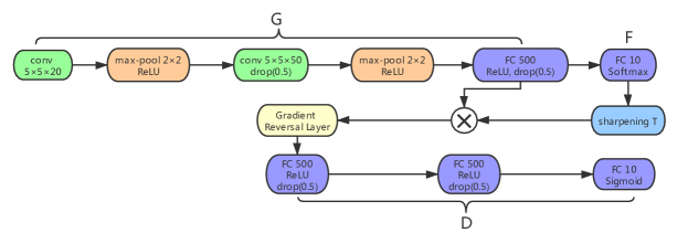
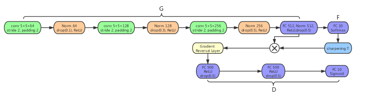
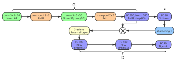
More precisely, four different architectures of are used in our experiments (as shown in figures 5, 6, 7, 8). In task, we adopt the the structure provided in MT [76]. For and tasks, we use the LeNet provided in CDAN [19]. For , and tasks, we use the DTN provided in CDAN [19]. In task, we adopt the the structure provided in DANN [18].
We follow the standard protocols for unsupervised domain adaptation and compare the average classification accuracy based on random experiments. For each experiment, we take the result of the last epoch.
The batch size is set to and we train epochs. SGD optimizer (momentum= , weight_decay= ) is with an initial learning rate of in the adversarial network and in the classifier. In sharpening function , is set to . For other special parameters in baselines, we all follow the original settings. We implement all methods with default parameters by PyTorch. The code of CLARINET is available at github.com/Yiyang98/BFUDA.
| Amount of of true-label source data | ||||||
|---|---|---|---|---|---|---|
| Tasks | 0 | 200 | 400 | |||
| true only | com only | true only | com+true | true only | com+true | |
| - | 47.0831.395 | 11.8390.019 | 49.4081.776 | 13.8751.366 | 49.5531.362 | |
| - | 83.6920.928 | 74.1801.218 | 88.5841.040 | 79.2000.837 | 89.4801.660 | |
| - | 94.5380.292 | 78.0111.473 | 93.2041.398 | 83.2041.545 | 94.6770.576 | |
| - | 63.0701.990 | 25.7720.146 | 64.7342.096 | 41.2321.089 | 64.9120.928 | |
| - | 71.7171.262 | 59.4141.381 | 70.7301.620 | 59.8050.951 | 71.1980.623 | |
| - | 97.0400.212 | 49.2321.354 | 97.1820.383 | 60.6401.570 | 97.2420.117 | |
| - | 84.4990.537 | 23.0091.102 | 84.2690.814 | 49.1201.236 | 85.5380.596 | |
| Average | - | 77.377 | 45.922 | 78.302 | 55.297 | 78.943 |
| Tasks | 600 | 800 | 1000 | |||
| true only | com+true | true only | com+true | true only | com+true | |
| 17.7222.626 | 50.8970.969 | 19.2780.853 | 51.0581.737 | 20.9721.061 | 53.2971.655 | |
| 82.5320.859 | 90.3581.938 | 85.8000.621 | 91.1060.561 | 88.1841.280 | 93.3421.294 | |
| 83.9251.511 | 94.8390.254 | 85.8392.074 | 94.7960.104 | 85.6990.777 | 95.0220.280 | |
| 41.6800.525 | 67.8981.625 | 51.6520.850 | 70.4161.819 | 53.5001.872 | 70.4461.358 | |
| 63.7571.344 | 72.7320.947 | 65.1610.766 | 73.0501.264 | 68.5221.285 | 73.3360.727 | |
| 76.8021.649 | 97.1780.396 | 85.2861.363 | 96.8420.267 | 86.4701.646 | 96.9480.266 | |
| 67.9221.079 | 85.9211.098 | 67.7881.878 | 86.7720.291 | 74.6541.054 | 87.0240.542 | |
| Average | 62.049 | 79.975 | 65.829 | 80.577 | 68.286 | 81.345 |
| Methods | Average | |||||||
|---|---|---|---|---|---|---|---|---|
| C w/ | 6.4812.536 | 0.4550.722 | 0.0550.129 | 3.7080.688 | 7.0880.424 | 1.8320.102 | 1.2980.070 | 2.987 |
| C w/o | 41.9082.796 | 84.3021.127 | 93.3010.465 | 44.5002.088 | 70.9940.749 | 94.3820.150 | 83.4080.545 | 73.256 |
| C w/o | 43.0752.553 | 83.1921.796 | 93.4190.588 | 52.4381.927 | 72.1281.569 | 95.4421.004 | 83.0550.652 | 74.678 |
| CLARINET | 47.0831.395 | 83.6920.928 | 94.5380.292 | 63.0701.990 | 71.7171.262 | 97.0400.212 | 84.4990.537 | 77.377 |
VI-D Results on CC-UDA Tasks
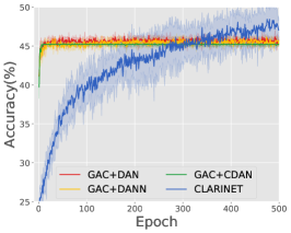
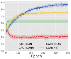
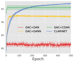
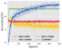
Table I reports the target-domain accuracy of methods on CC-UDA tasks. As can be seen, our CLARINET performs best on each task and the average accuracy of CLARINET is significantly higher than those of baselines. Compared with GAC method, CLARINET successfully transfers knowledge from complementary-label source data to unlabeled target data. Since CDAN has shown much better adaptation performance than DANN and DAN [19], GAC+CDAN should outperform other two-step methods on each task. However, on the task , the accuracy of GAC+CDAN is much lower than that of GAC+DANN. This abnormal phenomenon shows that the noise contained in pseudo-label source data significantly reduces transferability of existing UDA methods. Namely, we cannot obtain the reliable adaptation performance by using two-step CC-UDA approach.
. CIFAR and STL are 10-class object recognition datasets with colored images. We remove the non-overlapping classes (“frog” and “monkey”) and readjust the labels to align the two datasets. Namely this task reduce to a -class classification problem. Furthermore, we downscale the image dimesion of STL to match the dimension of CIFAR. As shown in Figure 4 (a), two-step methods could hardly realize knowledge transfer, while our CLARINET’s performance surpasses others by a comfortable margin.
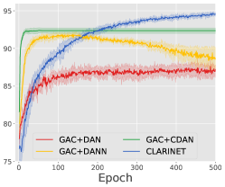
. MNIST and USPS are both grayscale digits images, thus the distribution discrepancy between the two tasks is relatively small. As shown in Figure 4 (b) and (c), in both adaptation directions, CARINET all achieve the best performance far above other baselines.
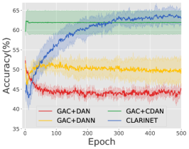
. SVHN and MNIST are both digit datasets. Whereas MNIST consists of black-and-white handwritten digits, SVHN consists of crops of colored, street house numbers. MNIST has a lower image dimensionality than SVHN, thus we adopt the dimension of MNIST to with three channels to match SVHN. Because of the above factors, the gap between two distributions are relatively larger compared to that of the . As shown in Figure 4 (d), GAC+CDAN perform much better than GAC+DAN and GAC+DANN, but still worse than our CLARINET.
. MNIST-M is a transformed dataset from MNIST, which was composed by merging clips of a background from the BSDS500 datasets [77]. For a human the classification task on MNIST-M only becomes slightly harder, whereas for a CNN network trained on MNIST, this domain is quite different, as the background and the strokes are no longer constant. As shown in Figure 4 (e), Our method is slightly more effective than GAC+CDAN and far more effective than the other two methods.
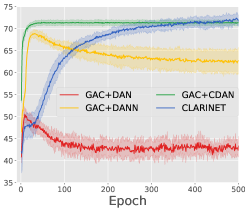
. This adaptation reflects a common adaptation problem of transferring from synthetic images to real images. The SYN-DIGITS dataset consists of a huge amount of data, generated from Windows fonts by varying the text, positioning, orientation, background, stroke color, and the amount of blur. As shown in Figure 4 (f), our method outperforms other baselines and achieves pretty high accuracy. Thus with sufficient source data, CLARINE could achieve excellent results.
. This adaptation is another common adaptation problem of transferring from synthetic images to real images, but is more challenging than in the case of the MNIST experiment. As shown in Figure 4 (g), our method is obviously more effective than other baselines. GAC+DANN does not apply to this task, achieving the lowest accuracy.
VI-E Results on PC-UDA Tasks
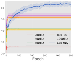
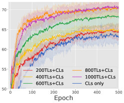
Table II reports the target-domain accuracy of CLARINET on PC-UDA tasks when we have different amount of true-label source data. “true only” means training on a certain number of true-label source data with ordinary UDA method. “com only” means training on complementary-label source data only with CLARINET. “com+true” stands for training on a certain number of true-label source data and complementary-label source data with CLARINET. In general, the accuracy of CLARINET increases when increasing the amount of true-label source data from to . Thus, it is proved that CLARINET can sufficiently leverage true-label source data to improve adaptation performance.
The improvement is especially evident on task and task. For task, this is probably because the dataset sample size of USPS is relatively small, true-label data actually has occupied a large part. For task, SVHN is complicated for complementary-label learning. Hence adding a small number of true-label data could help to train a more accurate classifier. This phenomenon also reminds us that for complex datasets, adding some true-label data to assist training would be pretty appropriate. On task, adding true-label source data does not bring significant improvement, which is most likely due to the result on complementary-label data is already relatively good and true-label source data is unable to assist in achieving better result.
We also compare the efficacy of true-label source data with complementary-label source data. Taking task as an example (shown in the left part of Figure 4 (h)), we compare the target-domain accuracy of ordinary UDA method trained with different amount of true-label source data and that of CLARINET trained with complementary-label source data only (“CLs Only”). The accuracy decreases significantly when reducing the amount of true-label source data, which suggests that sufficient true-label source data are inevitably required in UDA scenario. Then we compare the target-domain accuracy of CLARINET trained with complementary-label source data only with that of CLARINET trained with different amount of true-label and complementary-label source data. It is clear that CLARINET effectively uses two kinds of data to obtain better adaptation performance than using complementary-label source data only. Besides, as the number of true-label source data used increases, the classification accuracy becomes better (shown in the right part of Figure 4 (h)).
VI-F Ablation Study
Finally, we conduct experiments to show the contributions of different components in CLARINET. We consider following baselines:
C w/ uses the cross-entropy loss to take place of complementary-label loss. Actually, it stands for applying ordinary UDA methods directly on complementary-label based UDA tasks. The target-domain accuracy of C w/ will show whether UDA methods can address the complementary-label based UDA problem. C w/o train the domain discriminator only based on feature representations and , thus the result could indicate whether the conditional adversarial way could capture the multimodal structures so as to improve the transfer effect. Please notice, the sharpening function is useless in this network as it works on the label prediction and . Comparing CLARINET with C w/o reveals if the sharpening function takes effect.
As shown in Table III, the target-domain accuracy of C w/ is much lower than that of other methods. Namely, UDA methods cannot handle complementary-label based UDA tasks directly. Its result is not even as good as random classification, as the network is trained taking the wrong label as the target result. Comparing with C w/o , C w/o has a worse performance, which proves that the conditional adversarial way could really improve the transfer effect. Therefore, it is necessary to capture the multimodal structures of distributions with cross-covariance dependency between the features and classes in the field of adversarial based UDA. Although C w/o achieves better accuracy than other baselines, its accuracy still worse than CLARINET’s. The result reveals that the sharpening function helps to capture multimodal structures of distributions on basis of the characteristics of complementary-label learning. Thus, the sharpening function can improve the adaptation performance.
VII Conclusion and Further Study
This paper presents a new setting, complementary-label based UDA, which exploits economical complementary-label source data instead of expensive true-label source data. We consider two cases of the complementary-label based UDA, one is that the source domain only contains complementary-label data (CC-UDA), and the other is that the source domain has plenty of complementary-label data and a small amount of true-label data (PC-UDA). Since existing UDA methods cannot address complementary-label based UDA problem, we propose a novel, one-step approach, called complementary label adversarial network (CLARINET). CLARINET could handle both CC-UDA and PC-UDA tasks. Experiments conducted on complementary-label based UDA tasks confirm that CLARINET effectively achieves distributional adaptation from complementary-label source data to unlabeled target data and outperforms a series of competitive baselines. In the future, we plan to explore more effective ways to solve complementary-label based UDA and extend the application of complementary labels in domain adaptation.
Acknowledgements
The work presented in this paper was supported by the Australian Research Council (ARC) under FL190100149. The first author particularly thanks the support by UTS-CAI during her visit.
References
- [1] Y. Luo, Y. Wen, T. Liu, and D. Tao, “Transferring knowledge fragments for learning distance metric from a heterogeneous domain,” TPAMI, pp. 1013–1026, 2019.
- [2] M. Xiao and Y. Guo, “Feature space independent semi-supervised domain adaptation via kernel matching,” TPAMI, pp. 54–66, 2014.
- [3] K. Zhang, B. Schölkopf, K. Muandet, and Z. Wang, “Domain adaptation under target and conditional shift,” in ICML, 2013, pp. 819–827.
- [4] S. Motiian, M. Piccirilli, D. Adjeroh, and G. Doretto, “Unified deep supervised domain adaptation and generalization,” in ICCV, 2017, pp. 5715–5725.
- [5] S. Sukhija, N. Krishnan, and G. Singh, “Supervised heterogeneous domain adaptation via random forests.” in IJCAI, 2016, pp. 2039–2045.
- [6] E. Tzeng, J. Hoffman, T. Darrell, and K. Saenko, “Simultaneous deep transfer across domains and tasks,” in ICCV, 2015, pp. 4068–4076.
- [7] L. Cheng and S. J. Pan, “Semi-supervised domain adaptation on manifolds,” TNNLS, pp. 2240–2249, 2014.
- [8] S. Mehrkanoon and J. A. K. Suykens, “Regularized semipaired kernel CCA for domain adaptation,” TNNLS, pp. 3199–3213, 2018.
- [9] K. Islam, V. Hill, B. Schaeffer, R. Zimmerman, and J. Li, “Semi-supervised adversarial domain adaptation for seagrass detection in multispectral images,” in ICDM, 2019, pp. 1120–1125.
- [10] P. Wei, Y. Ke, and C. K. Goh, “Feature analysis of marginalized stacked denoising autoenconder for unsupervised domain adaptation,” TNNLS, pp. 1321–1334, 2019.
- [11] K. Saito, Y. Ushiku, and T. Harada, “Asymmetric tri-training for unsupervised domain adaptation,” in ICML, 2017, pp. 2988–2997.
- [12] Y. Cao, M. Long, and J. Wang, “Unsupervised domain adaptation with distribution matching machines,” in AAAI, 2018, pp. 2795–2802.
- [13] Z. Deng, Y. Luo, and J. Zhu, “Cluster alignment with a teacher for unsupervised domain adaptation,” in ICCV, 2019, pp. 9944–9953.
- [14] S. Zhao, H. Fu, M. Gong, and D. Tao, “Geometry-aware symmetric domain adaptation for monocular depth estimation,” in CVPR, 2019, pp. 9788–9798.
- [15] G. Agresti, H. Schäfer, P. Sartor, and P. Zanuttigh, “Unsupervised domain adaptation for tof data denoising with adversarial learning,” in CVPR, 2019, pp. 5584–5593.
- [16] M. Long, Y. Cao, J. Wang, and M. I. Jordan, “Learning transferable features with deep adaptation networks,” in ICML, 2015, pp. 97–105.
- [17] M. Long, H. Zhu, J. Wang, and M. I. Jordan, “Deep transfer learning with joint adaptation networks,” in ICML, 2017, pp. 2208–2217.
- [18] Y. Ganin, E. Ustinova, H. Ajakan, P. Germain, H. Larochelle, F. Laviolette, M. Marchand, and V. Lempitsky, “Domain-adversarial training of neural networks,” JMLR, pp. 1–35, 2016.
- [19] M. Long, Z. Cao, J. Wang, and M. Jordan, “Conditional adversarial domain adaptation,” in NeurIPS, 2018, pp. 1640–1650.
- [20] M. Gong, K. Zhang, T. Liu, D. Tao, C. Glymour, and B. Schölkopf, “Domain adaptation with conditional transferable components,” in ICML, 2016, pp. 2839–2848.
- [21] K. Zhang, M. Gong, and B. Schölkopf, “Multi-source domain adaptation: A causal view,” in AAAI, 2015, pp. 3150–3157.
- [22] S. Sankaranarayanan, Y. Balaji, C. Castillo, and R. Chellappa, “Generate to adapt: Aligning domains using generative adversarial networks,” in CVPR, 2018, pp. 8503–8512.
- [23] T. Ishida, G. Niu, W. Hu, and M. Sugiyama, “Learning from complementary labels,” in NeurIPS, 2017, pp. 5639–5649.
- [24] T. Ishida, G. Niu, A. Menon, and M. Sugiyama, “Complementary-label learning for arbitrary losses and models,” in ICML, 2019, pp. 2971–2980.
- [25] L. FENG, T. Kaneko, B. Han, G. Niu, B. An, and M. Sugiyama, “Learning with multiple complementary labels,” in ICML, 2020.
- [26] X. Yu, T. Liu, M. Gong, and D. Tao, “Learning with biased complementary labels,” in ECCV, 2018, pp. 69–85.
- [27] F. Liu, J. Lu, B. Han, G. Niu, G. Zhang, and M. Sugiyama, “Butterfly: A panacea for all difficulties in wildly unsupervised domain adaptation,” in NeurIPS LTS Workshop, 2019.
- [28] Y. Shu, Z. Cao, M. Long, and J. Wang, “Transferable curriculum for weakly-supervised domain adaptation,” in AAAI, 2019, pp. 4951–4958.
- [29] Y. Zhang, L. Feng, Z. Fang, B. Yuan, G. Zhang, and J. Lu, “Clarinet: A one-step approach towards budget-friendly unsupervised domain adaptation,” in IJCAI, 2020.
- [30] L. Song, J. Huang, A. Smola, and K. Fukumizu, “Hilbert space embeddings of conditional distributions with applications to dynamical systems,” in ICML, 2009, pp. 961–968.
- [31] R. Gopalan, R. Li, and R. Chellappa, “Domain adaptation for object recognition: An unsupervised approach,” in ICCV, 2011, pp. 999–1006.
- [32] B. Gong, Y. Shi, F. Sha, and K. Grauman, “Geodesic flow kernel for unsupervised domain adaptation,” in CVPR, 2012, pp. 2066–2073.
- [33] J. Hoffman, S. Guadarrama, E. Tzeng, R. Hu, J. Donahue, R. Girshick, T. Darrell, and K. Saenko, “Lsda: Large scale detection through adaptation,” in NeurIPS, 2014, pp. 3536–3544.
- [34] R. Collobert, J. Weston, L. Bottou, M. Karlen, K. Kavukcuoglu, and P. Kuksa, “Natural language processing (almost) from scratch,” JMLR, pp. 2493–2537, 2011.
- [35] X. Glorot, A. Bordes, and Y. Bengio, “Domain adaptation for large-scale sentiment classification: A deep learning approach,” in ICML, 2011, pp. 513–520.
- [36] J. Huang, A. Gretton, K. Borgwardt, B. Schölkopf, and A. J. Smola, “Correcting sample selection bias by unlabeled data,” in NeurIPS, 2007, pp. 601–608.
- [37] S. J. Pan, I. W. Tsang, J. T. Kwok, and Q. Yang, “Domain adaptation via transfer component analysis,” TNNLS, pp. 199–210, 2010.
- [38] Y. Bengio, A. Courville, and P. Vincent, “Representation learning: A review and new perspectives,” TPAMI, pp. 1798–1828, 2013.
- [39] J. Yosinski, J. Clune, Y. Bengio, and H. Lipson, “How transferable are features in deep neural networks?” in NeurIPS, 2014, pp. 3320–3328.
- [40] F. Liu, W. Xu, J. Lu, G. Zhang, A. Gretton, and D. J. Sutherland, “Learning deep kernels for non-parametric two-sample tests,” in ICML, 2020.
- [41] K. Bousmalis, N. Silberman, D. Dohan, D. Erhan, and D. Krishnan, “Unsupervised pixel-level domain adaptation with generative adversarial networks,” in CVPR, 2017, pp. 3722–3731.
- [42] K. Lee, X. He, L. Zhang, and L. Yang, “Cleannet: Transfer learning for scalable image classifier training with label noise,” in CVPR, 2018, pp. 5447–5456.
- [43] F. Schroff, A. Criminisi, and A. Zisserman, “Harvesting image databases from the web,” TPAMI, pp. 754–766, 2011.
- [44] Y. Zhang, T. Liu, M. Long, and M. Jordan, “Bridging theory and algorithm for domain adaptation,” in ICML, 2019, pp. 7404–7413.
- [45] Z. Fang, J. Lu, F. Liu, J. Xuan, and G. Zhang, “Open set domain adaptation: Theoretical bound and algorithm,” arXiv preprint arXiv:1907.08375, 2019.
- [46] M. Ghifary, D. Balduzzi, W. B. Kleijn, and M. Zhang, “Scatter component analysis: A unified framework for domain adaptation and domain generalization,” TPAMI, pp. 1414–1430, 2017.
- [47] A. Kumar, P. Sattigeri, and T. Fletcher, “Semi-supervised learning with gans: Manifold invariance with improved inference,” in NeurIPS, 2017, pp. 5534–5544.
- [48] B. Frénay and M. Verleysen, “Classification in the presence of label noise: A survey,” TNNLS, pp. 845–869, 2014.
- [49] Y. Li and Z. Zhou, “Towards making unlabeled data never hurt,” TPAMI, pp. 175–188, 2015.
- [50] T. Sakai, M. du Plessis, G. Niu, and M. Sugiyama, “Semi-supervised classification based on classification from positive and unlabeled data,” in ICML, 2017, pp. 2998–3006.
- [51] B. Han, Q. Yao, X. Yu, G. Niu, M. Xu, W. Hu, I. Tsang, and M. Sugiyama, “Co-teaching: Robust training of deep neural networks with extremely noisy labels,” in NeurIPS, 2018, pp. 8527–8537.
- [52] B. Han, J. Yao, G. Niu, M. Zhou, I. Tsang, Y. Zhang, and M. Sugiyama, “Masking: A new perspective of noisy supervision,” in NeurIPS, 2018, pp. 5836–5846.
- [53] Q. Miao, Y. Cao, G. Xia, M. Gong, J. Liu, and J. Song, “Rboost: Label noise-robust boosting algorithm based on a nonconvex loss function and the numerically stable base learners,” TNNLS, pp. 2216–2228, 2016.
- [54] E. Xing, M. Jordan, S. Russell, and A. Ng, “Distance metric learning with application to clustering with side-information,” in NeurIPS, 2003, pp. 521–528.
- [55] T. F. Covoes, E. R. Hruschka, and J. Ghosh, “Competitive learning with pairwise constraints,” TNNLS, pp. 164–169, 2013.
- [56] J. Goldberger, G. Hinton, S. Roweis, and R. Salakhutdinov, “Neighbourhood components analysis,” in NeurIPS, 2005, pp. 513–520.
- [57] M. Du Plessis, G. Niu, and M. Sugiyama, “Analysis of learning from positive and unlabeled data,” in NeurIPS, 2014, pp. 703–711.
- [58] G. Niu, M. du Plessis, T. Sakai, Y. Ma, and M. Sugiyama, “Theoretical comparisons of positive-unlabeled learning against positive-negative learning,” in NeurIPS, 2016, pp. 1199–1207.
- [59] C. Gong, T. Liu, J. Yang, and D. Tao, “Large-margin label-calibrated support vector machines for positive and unlabeled learning,” TNNLS, pp. 3471–3483, 2019.
- [60] R. Kiryo, G. Niu, M. du Plessis, and M. Sugiyama, “Positive-unlabeled learning with non-negative risk estimator,” in NeurIPS, 2017, pp. 1675–1685.
- [61] G. Agresti, H. Schaefer, P. Sartor, and P. Zanuttigh, “Unsupervised domain adaptation for tof data denoising with adversarial learning,” in CVPR, 2019, pp. 5584–5593.
- [62] I. Goodfellow, J. Pouget-Abadie, M. Mirza, B. Xu, D. Warde-Farley, S. Ozair, A. Courville, and Y. Bengio, “Generative adversarial nets,” in NeurIPS, 2014, pp. 2672–2680.
- [63] S. Arora, R. Ge, Y. Liang, T. Ma, and Y. Zhang, “Generalization and equilibrium in generative adversarial nets (gans),” in ICML, 2017, pp. 224–232.
- [64] M. Mirza and S. Osindero, “Conditional generative adversarial nets,” CoRR, 2014.
- [65] A. Odena, C. Olah, and J. Shlens, “Conditional image synthesis with auxiliary classifier gans,” in ICML, 2017, pp. 2642–2651.
- [66] I. Goodfellow, Y. Bengio, and A. Courville, Deep learning. MIT press, 2016.
- [67] D. Berthelot, N. Carlini, I. Goodfellow, N. Papernot, A. Oliver, and C. A. Raffel, “Mixmatch: A holistic approach to semi-supervised learning,” in NeurIPS, 2019, pp. 5050–5060.
- [68] X. Zhu, Z. Ghahramani, and J. Lafferty, “Semi-supervised learning using gaussian fields and harmonic functions,” in ICML, 2003, pp. 912–919.
- [69] A. Krizhevsky, G. Hinton et al., “Learning multiple layers of features from tiny images,” Master’s thesis, 2009.
- [70] A. Coates, A. Ng, and H. Lee, “An analysis of single-layer networks in unsupervised feature learning,” in AISTATS, 2011, pp. 215–223.
- [71] Y. LeCun, L. Bottou, Y. Bengio, and P. Haffner, “Gradient-based learning applied to document recognition,” Proceedings of the IEEE, pp. 2278–2324, 1998.
- [72] T. Hastie, J. Friedman, and R. Tibshirani, The Elements of Statistical Learning: Data Mining, Inference, and Prediction, 2001.
- [73] Y. Netzer, T. Wang, A. Coates, A. Bissacco, B. Wu, and A. Ng, “Reading digits in natural images with unsupervised feature learning,” in NeurIPS DLUFL Workshop, 2011.
- [74] Y. Ganin and V. Lempitsky, “Unsupervised domain adaptation by backpropagation,” in ICML, 2015, pp. 1180–1189.
- [75] R. Shu, H. Bui, H. Narui, and S. Ermon, “A DIRT-T approach to unsupervised domain adaptation,” in ICLR, 2018.
- [76] G. French, M. Mackiewicz, and M. Fisher, “Self-ensembling for visual domain adaptation,” in ICLR, 2018.
- [77] P. Arbelaez, M. Maire, C. Fowlkes, and J. Malik, “Contour detection and hierarchical image segmentation,” TPAMI, pp. 898–916, 2010.
![[Uncaptioned image]](/html/2008.01454/assets/zhangyiyang3.jpg) |
Yiyang Zhang received her B.E. degree in Automation from Tsinghua University, P.R. China, in 2018. She is currently a Master student in Data Science at Shenzhen International Graduate School, Tsinghua University, and a visiting student with the Centre for Artificial Intelligence (CAI), the University of Technology, Sydney (UTS). Her research interests include transfer learning and domain adaptation. |
![[Uncaptioned image]](/html/2008.01454/assets/Feng_Liu.jpg) |
Feng Liu is a Doctoral candidate in Centre for Artificial intelligence, Faculty of Engineering and Information Technology, University of Technology Sydney, Australia. He received an M.Sc. degree in probability and statistics and a B.Sc. degree in pure mathematics from the School of Mathematics and Statistics, Lanzhou University, China, in 2015 and 2013, respectively. His research interests include domain adaptation and two-sample test. He has served as a senior program committee member for ECAI and program committee members for NeurIPS, ICML, IJCAI, CIKM, FUZZ-IEEE, IJCNN and ISKE. He also serves as reviewers for TPAMI, TNNLS, TFS and TCYB. He has received the UTS-FEIT HDR Research Excellence Award (2019), Best Student Paper Award of FUZZ-IEEE (2019) and UTS Research Publication Award (2018). |
![[Uncaptioned image]](/html/2008.01454/assets/ZhenFang.jpg) |
Zhen Fang received his M.Sc. degree in pure mathematics from the School of Mathematical Sciences Xiamen University, Xiamen, China, in 2017. He is working toward a PhD degree with the Faculty of Engineering and Information Technology, University of Technology Sydney, Australia. His research interests include transfer learning and domain adaptation. He is a Member of the Decision Systems and e-Service Intelligence (DeSI) Research Laboratory, CAI, University of Technology Sydney. |
![[Uncaptioned image]](/html/2008.01454/assets/yuanbo2.jpg) |
Bo Yuan received the B.E. degree from Nanjing University of Science and Technology, P.R.China, in 1998, and the M.Sc. and Ph.D. degrees from The University of Queensland (UQ), Australia, in 2002 and 2006, respectively, all in Computer Science. From 2006 to 2007, he was a Research Officer on a project funded by the Australian Research Council at UQ. He is currently an Associate Professor in the Division of Informatics, Shenzhen International Graduate School, Tsinghua University, and a member of the Intelligent Computing Lab. His research interests include Intelligent Computing and Pattern Recognition. |
![[Uncaptioned image]](/html/2008.01454/assets/A-guangquan-zhang.jpg) |
Guangquan Zhang is a Professor and Director of the Decision Systems and e-Service Intelligent (DeSI) Research Laboratory, Faculty of Engineering and Information Technology, University of Technology Sydney, Australia. He received his PhD in applied mathematics from Curtin University of Technology, Australia, in 2001. His research interests include fuzzy machine learning, fuzzy optimization, and machine learning and data analytics. He has authored four monographs, five textbooks, and 350 papers including 160 refereed international journal papers. Dr. Zhang has won seven Australian Research Council (ARC) Discovery Project grants and many other research grants. He was awarded an ARC QEII Fellowship in 2005. He has served as a member of the editorial boards of several international journals, as a guest editor of eight special issues for IEEE Transactions and other international journals, and has co-chaired several international conferences and work-shops in the area of fuzzy decision-making and knowledge engineering. |
![[Uncaptioned image]](/html/2008.01454/assets/JieLu.jpg) |
Jie Lu (F’18) is a Distinguished Professor and the Director of the Centre for Artificial Intelligence at the University of Technology Sydney, Australia. She received her PhD degree from Curtin University of Technology, Australia, in 2000. Her main research interests arein the areas of fuzzy transfer learning, concept drift, decision support systems, and recommender systems. She is an IEEE fellow, IFSA fellow and Australian Laureate fellow. She has published six research books and over 450 papers in refereed journals and conference proceedings; has won over 20 ARC Laureate, ARC Discovery Projects, government and industry projects. She serves as Editor-In-Chief for Knowledge-Based Systems (Elsevier) and Editor-In-Chief for International journal of computational intelligence systems. She has delivered over 25 keynote speeches at international conferences and chaired 15 international conferences. She has received various awards such as the UTS Medal for Research and Teaching Integration (2010), the UTS Medal for Research Excellence (2019), the Computer Journal Wilkes Award (2018), the IEEE Transactions on Fuzzy Systems Outstanding Paper Award (2019), and the Australian Most Innovative Engineer Award (2019). |