The multipolar structure of fuzzballs

Abstract

We extend and refine a general method to extract the multipole moments of arbitrary stationary spacetimes and apply it to the study of a large family of regular horizonless solutions to ${\cal N}{\,=\,}2$ four-dimensional supergravity coupled to four Abelian gauge fields. These microstate geometries can carry angular momentum and have a much richer multipolar structure than the Kerr black hole. In particular they break the axial and equatorial symmetry, giving rise to a large number of nontrivial multipole moments. After studying some analytical examples, we explore the four-dimensional parameter space of this family with a statistical analysis. We find that microstate mass and spin multipole moments are typically (but not always) larger that those of a Kerr black hole with the same mass and angular momentum. Furthermore, we find numerical evidence that some invariants associated with the (dimensionless) moments of these microstates grow monotonically with the microstate size and display a global minimum at the black-hole limit, obtained when all centers collide. Our analysis is relevant in the context of measurements of the multipole moments of dark compact objects with electromagnetic and gravitational-wave probes, and for observational tests to distinguish fuzzballs from classical black holes.

1 Introduction

Within classical General Relativity (GR) a series of theorems Carter71 ; Hawking:1973uf ; Heusler:1998ua ; Chrusciel:2012jk ; Robinson state that the unique vacuum, stationary solution is the Kerr metric Kerr:1963ud , which is therefore believed to provide a reliable description of the spacetime around any dark compact object formed after gravitational collapse.

Any stationary Black Hole (BH) in isolation is axisymmetric. As a result the only non-vanishing mass (current) multipole moments are $\mathcal{M}_{\ell}=\mathcal{M}_{\ell m=0}$ ($\mathcal{S}_{\ell}=\mathcal{S}_{\ell m=0}$), that satisfy the elegant relation Geroch:1970cd ; Hansen:1974zz

$$\mathcal{M}_{\ell}+{\rm i}\mathcal{S}_{\ell}=\mathcal{M}^{\ell+1}\left({\rm i}\chi\right)^{\ell}\,,$$ (1.1)

where $\mathcal{M}={\cal M}_{0}$ is the BH mass, $\mathcal{J}=\mathcal{S}_{1}$ the angular momentum, and $\chi\equiv{\mathcal{J}}/{\mathcal{M}^{2}}$ the dimensionless spin. Equatorial symmetry of the Kerr metric implies ${\cal M}_{\ell}=0$ (${\cal S}_{\ell}=0$) when $\ell$ is odd (even), and the specific spin dependence of the non-vanishing moments, ${\cal M}_{\ell}\propto\chi^{\ell}$ and ${\cal S}_{\ell}\propto\chi^{\ell}$. This peculiarity of the Kerr metric is not enjoyed by other compact-object solutions in GR Pani:2015tga ; Uchikata:2015yma ; Uchikata:2016qku ; Raposo:2018xkf , neither by BHs in other gravitational theories Psaltis:2008bb ; Yunes:2013dva ; Berti:2015itd .

Measuring (at least three) properties of an astrophysical dark object, such as mass, spin, and the mass quadrupole $\mathcal{M}_{2}$, may provide null-hypothesis tests of the Kerr metric and as consequence of Einstein’s gravity in the strong-field regime Psaltis:2008bb ; Gair:2012nm ; Yunes:2013dva ; Berti:2015itd ; Cardoso:2016ryw ; Barack:2018yly ; Cardoso:2019rvt . This adds to other observational tests of fuzzballs that have been recently proposed, see, e.g., Refs. Hertog:2017vod ; Guo:2017jmi . Quite intriguingly, the current gravitational-wave observations (especially the recent GW190814 Abbott:2020khf and GW190521 Abbott:2020tfl ; Abbott:2020mjq ) have not yet excluded the possible existence of exotic compact objects other than BHs and neutron stars.

According to the cosmic censorship conjecture, curvature singularities in GR are believed to be covered by event horizons Penrose:1969pc ; Wald:1997wa ; Penrose_CCC . A consistent quantum theory of gravity should be able to resolve or smoothen BH singularities and to provide a microscopical interpretation of the BH thermodynamical properties, such as entropy and temperature, related to the area of the event horizon and its surface gravity, respectively Bekenstein ; Hawking:1976de . Furthermore, BH evaporation through the emission of Hawking radiation Hawking:1974sw leads to other paradoxes, that can be addressed in a consistent quantum theory of gravity such as string theory.

In this framework, BHs can be represented as bound-states of strings and D-branes intersecting point-wise along the spacetime. Extremal (charged BPS) BHs can be successfully described and a precise microscopic account of the entropy can be given through the counting of light excitations of the open strings connecting the various branes Strominger:1996sh ; Horowitz:1996ay ; Maldacena:1997de .

The information-loss paradox and the singularity problem Penrose:1969pc ; Wald:1997wa ; Penrose_CCC in GR can be solved in string theory relying on the “fuzzball” proposal Lunin:2001jy ; Lunin:2002qf ; Mathur:2005zp ; Mathur:2008nj ; Mathur:2009hf . From this vantage point, BH microstates are associated to smooth horizonless geometries with the same asymptotics (mass, charges, and angular momenta). Classical properties of BHs emerge as a result of a coarse-graining averaging procedure or as a ‘collective behavior’ of fuzzballs Bianchi:2017sds ; Bianchi:2018kzy ; Bena:2018mpb ; Bena:2019azk ; Bianchi:2020des . Unfortunately, so far, finding a statistically significant fraction for five-dimensional (3-charge) and for four-dimensional (4-charge) BPS BHs have proven to be too challenging of a task. Only a limited class of microstate geometries have been found, using multi-center or stratum ansatze Bena:2015bea ; Bena:2016agb ; Bena:2016ypk ; Bena:2017xbt ; Bianchi:2017bxl ; Bena:2017upb , that can be embedded in a consistent quantum theory of gravity such as string theory Giusto:2009qq ; Giusto:2011fy ; Bianchi:2016bgx . Very little or nothing is known at the moment about microstates of neutral and non-BPS BHs.

Furthermore, not much has been done to investigate the phenomenological consequences of the fuzzball proposal and to identify observables that can distinguish an ensemble of microstates from the classical BH picture or from other exotic compact objects which are still viable hypothesis. In particular, the measured masses of the binary components of GW190814 Abbott:2020khf and of GW190521 Abbott:2020tfl ; Abbott:2020mjq look incompatible with the standard astrophysical formation scenario for BHs, being either too light (as in the case of the lighest body in GW190814) or too massive (as it seems the case for at least one of the bodies in GW190521). Thus, testing the “Kerr hypothesis” is an urgent cornerstone of strong-field verifications of gravity, based on different observations with both electromagnetic and gravitational-wave probes Psaltis:2008bb ; Gair:2012nm ; Yunes:2013dva ; Berti:2015itd ; Cardoso:2016ryw ; Barack:2018yly ; Cardoso:2019rvt .

The scope of this paper (a companion of a recent letter Bianchi:2020bxa ) is to study one specific aspect of fuzzballs that can be used to distinguish microstates geometries from their classical BH counterpart. Namely, we shall study the multipolar structure, which inter alia affects the motion of test particles around a central object, the inspiral of a binary system, and therefore the electromagnetic signal from accreting dark compact objects Psaltis:2008bb and the gravitational-wave signal emitted by coalescing binaries Blanchet:2006zz . Studying the multipolar structure of fuzzballs is particularly interesting for two reasons:

• As argued in Bianchi:2020bxa , the multipolar structure of a fuzzball is significantly richer than that of a Kerr BH. While the latter is equatorial and axial symmetric, a microstate geometry can generically break any symmetry. This results in new classes of multipole moments which are identically zero in the Kerr case Raposo:2018xkf . Furthermore, as dictated by the no-hair theorem Heusler:1998ua ; Chrusciel:2012jk ; Robinson , all properties of a Kerr BH – including of course its infinite tower of multipole moments – are determined in terms of its mass ${\cal M}$ and angular momentum ${\cal J}$. Therefore, measuring independently three arbitrary multipole moments (typically the mass, spin, and the mass quadrupole moment) can place a strong constraint on alternatives to the classical Kerr picture Psaltis:2008bb ; Gair:2012nm ; Yunes:2013dva ; Berti:2015itd ; Cardoso:2016ryw ; Barack:2018yly ; Raposo:2018xkf ; Cardoso:2019rvt .

• At variance with other observables, the multipole moments have the advantage of being easy to calculate, since they require only an asymptotic expansion of the metric. This is particularly convenient in the context of fuzzballs, since the latter are typically described by very complicated metrics. Furthermore, although microstate geometries are manifestly regular when lifted to higher dimensions, they appear singular in four dimensions, the singularity being compensated by some divergence of the scalar fields emerging from the sanctification. Although harmless from a physical point of view, this singularity (as well as the lack of symmetries) complicates some phenomenological studies, for example the computation of the quasi-normal modes of these solutions. On the contrary, the multipole moments are extracted at asymptotic infinity, where the solution is manifestly regular also in four spacetime dimensions.

In this work we provide full details of the computation presented in Ref. Bianchi:2020bxa and extend that analysis to other, more general, solutions. While our approach is general and applies to any multi-center microstate geometry, we shall focus mostly on three-center solutions. As we shall show, the four-dimensional parameter space of this family is very rich. We identify some invariants associated with the multipole moments and employ a statistical analysis to compare the multipole moments of random microstate geometries with: a) those of a Kerr BH with the same mass and angular momentum; and b) those of the corresponding solution in the (non-rotating) BH limit, which is obtained when all centers collide on a point. In the former case we find that about $90\%$ of the solutions have invariant moments larger than Kerr, whereas in the latter case the invariants appear to be always larger than the corresponding quantities in the BH limit. Moreover these invariants grow always monotonically with the size (average distance between the centers) of the microstate. These properties are analogous to the fact that the quasi-normal mode exponential decay rate (the Lyapunov exponent of unstable null geodesics near the photon sphere) is maximum for the BH solution Bianchi:2020des and provide a portal to test the fuzzball proposal phenomenologically.

2 Multipole moments of generic stationary spacetime

In this section, we introduce two equivalent definitions of the multipole moments which can be directly applied to generic stationary and asymptotically flat metrics with no extra symmetry.

2.1 Multipole moments of the metric

We consider stationary asymptotically flat geometries in four dimensions. In an asymptotically Cartesian mass centered (ACMC) system, the metric of a stationary asymptotically flat object can be written as Bianchi:2020bxa

$$ds^{2}=dt^{2}(-1+c_{00})+c_{0i}\,dt\,dx_{i}+(1+c_{00})\,dx_{i}^{2}+\ldots$$ (2.1)

with $c_{00}$ and $c_{0i}$ harmonic functions admitting a harmonic expansion of the form

$$c_{00} {\,=\,}2\sum_{\ell=0}^{\infty}\sum_{m=-\ell}^{\ell}\frac{1}{r^{1+\ell}}\sqrt{\frac{4\pi}{2\ell{\,+\,}1}}{\cal M}_{\ell m}Y_{\ell m}$$ (2.2)

$$c_{0i} {\,=\,}2\sum_{\ell=1}^{\infty}\sum_{m=-\ell}^{\ell}\frac{1}{r^{1+\ell}}\sqrt{\frac{4\pi(\ell{\,+\,}1)}{\ell(2\ell{\,+\,}1)}}{\cal S}_{\ell m}Y^{B}_{i;\ell m}$$

in terms of the scalar ($Y_{lm}$) and axial vector ($Y^{B}_{i;\ell m}$) spherical harmonics. In (2.1) and thereafter the dots stand for terms involving spherical harmonics with $\ell^{\prime}<\ell$ at order $r^{-(1+\ell)}$ in the expansion.

We use the following definition for the scalar spherical harmonics

$$Y_{\ell m}=\sqrt{\frac{2\ell+1}{4\pi}\frac{(\ell-m)!}{(\ell+m)!}}e^{im\phi}P_{\ell m}(\cos\theta)$$ (2.3)

where $P_{\ell m}(x)$ are the associated Legendre polynomials

$$P_{\ell m}(x)=\left\{\begin{aligned} &\frac{(-)^{m}(1-x^{2})^{m/2}}{2^{\ell}\ell!}\frac{d^{\ell+m}}{dx^{\ell+m}}(x^{2}-1)^{\ell}\quad,\quad~{}~{}~{}~{}~{}m\geq 0\\ &\frac{(\ell+m)!}{(\ell-m)!}\frac{(1-x^{2})^{-m/2}}{2^{\ell}\ell!}\frac{d^{\ell-m}}{dx^{\ell-m}}(x^{2}-1)^{\ell}\quad,\quad m<0\end{aligned}\right.$$ (2.4)

For the sake of generality we give here the definition of the (radial, electric, and magnetic) vector spherical harmonics

$$Y^{R}_{i;\ell m}=n_{i}Y_{\ell m}\,.\qquad,\qquad Y^{E}_{i;\ell m} =\frac{r\partial_{i}Y_{\ell m}}{\sqrt{\ell(\ell+1)}}\qquad,\qquad Y^{B}_{i;\ell m}=\frac{\epsilon_{ijk}\,n_{j}\,r\partial_{k}Y_{\ell m}}{\sqrt{\ell(\ell+1)}}$$ (2.5)

The expansion coefficients ${\cal M}_{\ell m}$ and ${\cal S}_{\ell m}$ in Eq. (2.2) are the mass and current multipole moments of the spacetime, respectively. They can be conveniently packed into a single complex harmonic function defined as

$$H =H_{1}+{\rm i}\,H_{2}=\sum_{\ell=0}^{\infty}\sum_{m=-\ell}^{\ell}\frac{1}{r^{1+\ell}}\sqrt{\frac{4\pi}{2\ell+1}}\left({\cal M}_{\ell m}+{\rm i}\,{\cal S}_{\ell m}\right)Y_{\ell m}\,.$$ (2.6)

In terms of these variables the ACMC metric (2.1) can be written in the form

$$ds^{2} =-e^{-2H_{1}}(dt+\omega)^{2}+e^{2H_{1}}dx_{i}^{2}+\ldots$$ (2.7)

$$*_{3}d\omega =\epsilon_{ijk}\partial_{k}c_{0j}dx^{i}+\ldots=2\,dH_{2}+\ldots$$

with dots standing again for lower harmonics.

For axi-symmetric solutions (like the Kerr metric) it is convenient to rotate the coordinate axes so that the angular momentum vector is aligned with the $z$-axis. In this case the spherical harmonics with $m\neq 0$ vanish and one can write (defining from brevity ${\cal M}_{\ell 0}\equiv{\cal M}_{\ell}$ and likewise for the current moments)

$$H =\sum_{\ell=0}^{\infty}\frac{1}{r^{1+\ell}}\left({\cal M}_{\ell}+{\rm i}\,{\cal S}_{\ell}\right)P_{\ell}(\cos\theta)\,.$$ (2.8)

2.2 Multipolar expansion of the Killing one-form associated to stationarity

The mass (${\cal M}_{\ell m}$) and spin (${\cal S}_{\ell m}$) multipole moments can be alternatively viewed as the “electric” and “magnetic” spherical harmonic expansion coefficients of the Killing one-form $K=g_{t\mu}dx^{\mu}$ associated to the Killing vector $\partial_{t}$ of the stationary spacetime. Indeed, inverting formulae (2.2) one finds

$$\mathcal{M}_{\ell m} =\frac{\sqrt{2\ell+1}}{2(\ell+1)\sqrt{4\pi}}\,\lim_{r\to\infty}\,r^{\ell}\int Y_{\ell m}^{*}*dK$$ (2.9)

$$\mathcal{S}_{\ell m} =-\frac{\sqrt{2\ell+1}}{2(\ell+1)\sqrt{4\pi}}\,\lim_{r\to\infty}\,r^{\ell}\int Y_{\ell m}^{*}dK$$

where we used $\nabla^{2}_{S_{2}}Y_{\ell m}=-\ell(\ell+1)Y_{\ell m}$. Mass and angular momentum can be read off from the lower multipole moments

$$\mathcal{M}=\mathcal{M}_{00}\,,\qquad|\mathbfcal{J}|=\sqrt{\left|\mathcal{S}_{10}\right|^{2}+\left|\mathcal{S}_{11}\right|^{2}+\left|\mathcal{S}_{1-1}\right|^{2}}\,.$$ (2.10)

For later convenience, we introduce the dimensionless ratios

$$\overline{\mathcal{M}}_{\ell m}=\frac{\mathcal{M}_{\ell m}}{\mathcal{M}^{\ell+1}}\quad,\quad\overline{\mathcal{S}}_{\ell m}=\frac{\mathcal{S}_{\ell m}}{\mathcal{M}^{\ell+1}}\,,$$ (2.11)

and the dimensionless spin parameter, $\chi={\cal J}/{\cal M}^{2}$.

2.3 Multipolar structure of the Kerr(-Newman) metric

Although the multipolar structure of the neutral Kerr and charged Kerr-Newman BHs coincide Sotiriou:2004ud , here we review the most generic case of the Kerr-Newman solution. In the Boyer-Lindquist (BL) $\{t,\hat{r},\hat{\theta},\phi\}$ coordinates the metric and gauge field describing the Kerr-Newman solution can be written as

$$ds^{2} =-(1{-}\Delta_{t})dt^{2}-2a\sin^{2}\theta\Delta_{t}dt\,d\phi+\frac{\Sigma}{\Delta_{r}}dr^{2}+\Sigma d\hat{\theta}^{2}+\frac{\sin^{2}\hat{\theta}}{\Sigma}\left[(\hat{r}^{2}{+}a^{2})^{2}-a^{2}\Delta_{r}\sin^{2}\hat{\theta}\right]d\phi^{2}$$

$$A =-\frac{Q\hat{r}}{\Sigma}(dt-a\sin^{2}\hat{\theta}\,d\phi)-\frac{P\cos\hat{\theta}}{\Sigma}[a\,dt-(a^{2}+\hat{r}^{2})\,d\phi]\,,$$ (2.12)

where

$$\Sigma=\hat{r}^{2}+a^{2}\cos^{2}\hat{\theta}\quad,\quad\Delta_{t}=\frac{2{\cal M}\hat{r}-(Q^{2}+P^{2})}{\Sigma}\quad,\quad\Delta_{r}=\hat{r}^{2}-2{\cal M}\,\hat{r}+a^{2}+Q^{2}+P^{2}\,.$$ (2.13)

This solution is characterised by the mass ${\cal M}$, electric and magnetic charges $Q$ and $P$, and angular momentum ${\cal J}=a{\cal M}$ defined as

$${\cal M} =\frac{1}{8\pi}\int_{S^{2}_{\infty}}\!\!*dK\quad,\quad{\cal J}=-\frac{3}{16\pi}\lim_{r\to\infty}\int_{S^{2}_{r}}\!\!r\cos\theta\,dK=aM$$ (2.14)

$$Q =\frac{1}{4\pi}\int_{S^{2}_{\infty}}\!\!*F~{}~{}\quad,\quad P=\frac{1}{4\pi}\int_{S^{2}_{\infty}}\!\!F\,.$$

Inner and outer horizons exist for masses satisfying ${\cal M}^{2}\geq Q^{2}+P^{2}+a^{2}$ and are located at $\hat{r}_{\pm}={\cal M}\pm\sqrt{{\cal M}^{2}-a^{2}-Q^{2}-P^{2}}$. A curvature singularity is found at $\Sigma=0$. The area of the BH horizon is $A_{H}=4\pi(\hat{r}_{+}^{2}+a^{2})$.

The Kerr-Newman metric in the BL coordinates is not in the ACMC form. Indeed, in spherical coordinates a metric in the ACMC form can be written as

$$ds^{2}=g_{\mu\nu}dx^{\mu}dx^{\nu}=e^{a}\,e^{b}(\eta_{ab}+c_{ab})\qquad,\qquad e^{a}=(dt,dr,rd\theta,r\sin\theta d\phi)\,,$$ (2.15)

with $c_{ab}$ such that only harmonics of order at most $\ell$ at order $r^{-\ell+1}$ are present. It is easy to see that $c_{\hat{r}\hat{r}}$ and $c_{\hat{\theta}\hat{\theta}}$ in the Kerr-Newman metric in BL coordinates fail to meet this requirement. To bring the metric to the ACMC form one can perform the coordinate transformation

$$r^{2}=(\hat{r}-{\cal M})^{2}+a^{2}\sin^{2}\hat{\theta}\qquad,\qquad r\cos\theta=(\hat{r}-{\cal M})\cos\hat{\theta}\,,$$ (2.16)

which reduces to the (perturbative) result found by Hartle and Thorne Hartle:1968si to second order in the spin.

In the new variables one finds the non-vanishing components

$$c_{00} =c_{rr}=c_{\theta\theta}=c_{\phi\phi}={2{\cal M}\over r}\sum_{n=0}^{\infty}(-)^{n}{a^{2n}\over r^{2n}}P_{2n}(\cos\theta)+\ldots$$

$$c_{0\phi} ={2a{\cal M}\over r^{2}}\sum_{n=0}^{\infty}(-)^{n}{a^{2n}\over r^{2n}}{\partial_{\theta}P_{2n-1}(\cos\theta)\over 2n-1}+\ldots$$ (2.17)

leading to Hansen:1974zz ; Geroch:1970cd

$$\mathcal{M}_{2n}=(-1)^{n}a^{2n}{\cal M}\qquad,\qquad\mathcal{S}_{2n+1}=(-1)^{n}a^{2n+1}{\cal M}.$$ (2.18)

The mass and current multipole moments combine into the single complex harmonic function

$$H_{\rm Kerr}=\sum_{\ell=0}^{\infty}\left(\mathcal{M}_{\ell}+{\rm i}\,\mathcal{S}_{\ell}\right)\,\frac{P_{\ell}}{r^{1+\ell}}=\frac{{\cal M}}{\sqrt{x_{1}^{2}+x_{2}^{2}+(x_{3}-{\rm i}a)^{2}}}$$ (2.19)

We notice that real and imaginary parts of $H_{\rm Kerr}$ are given in terms of a sort of analytic continuation of a two-center harmonic function with centers located at $\pm ia$. In particular the mass is ${\cal M}$ and the angular momentum ${\cal J}=a{\cal M}$. The Schwarzschild solution is obtained by sending $a\to 0$ and the two centers coincide at the origin.

Finally, note that the multipole moments of the Kerr-Newman metric, Eq. (2.18), do not depend explicitly on the charges, so they are the same in the neutral (Kerr) limit Sotiriou:2004ud . Obviously the same holds true for Reissner-Nordström (the $\chi\to 0$ limit of Kerr-Newman), whose multipolar structure is the same as for Schwarzschild. More generally, the presence of minimally coupled scalar and gauge fields, equipped with energy momentum tensors dying faster than $1/r^{3}$ at infinity, does not destroy the Ricci flatness of the leading harmonic part of the ACMC metric (and hence it does not affect the way multipole moments can be extracted), but nevertheless results in a very different (from Kerr) multipolar structure.

3 Fuzzball solutions and their multipolar structure

Fuzzball solutions can be viewed as multi-center generalizations of the single center Schwarzschild and two-center Kerr metrics. In this section we review a family of solutions and discuss their multipolar structure.

3.1 The metric

In the framework of ${\cal N}=2$ four-dimensional supergravity, we consider gravity minimally coupled to four Maxwell fields and three complex scalars. A general class of extremal solutions of the Maxwell-Einstein-scalar system is described by a metric of the form Bena:2007kg ; Gibbons:2013tqa ; Bates:2003vx

$$ds^{2}=-e^{2U}\left(dt+\omega\right)^{2}+e^{-2U}\sum_{i=1}^{3}dx^{2}_{i},$$ (3.1)

with

$$e^{-4U}{=}VL_{1}L_{2}L_{3}{-}K^{1}K^{2}K^{3}M{+}{\textstyle\frac{1}{2}}\sum_{I>J}^{3}K^{I}K^{J}L_{I}L_{J}{-}{MV\over 2}\sum_{I=1}^{3}K^{I}L_{I}{-}{M^{2}V^{2}\over 4}{-}{\textstyle\frac{1}{4}}\sum_{I=1}^{3}(K^{I}L_{I})^{2}$$ (3.2)

$$*_{3}d\omega=\frac{1}{2}\left(VdM-MdV+K_{I}dL_{I}-L_{I}dK_{I}\right)$$ (3.3)

and $\{V,L_{I},K^{I},M\}$ eight harmonic functions, $I=1,2,3$. We consider $N$-center harmonic functions

$$V = v_{0}+\sum_{a=1}^{N}{v_{a}\over r_{a}}\qquad,\qquad L_{I}={\ell}_{0I}+\sum_{a=1}^{N}{{\ell}_{I,a}\over r_{a}}$$

$$K^{I} = k^{I}_{0}+\sum_{a=1}^{N}{k^{I}_{a}\over r_{a}}\qquad,\qquad M=m_{0}+\sum_{a=1}^{N}{m_{a}\over r_{a}}$$ (3.4)

with $r_{a}=|{\bf x}-{\bf x}_{a}|$ and ${\bf x}_{a}$ the position of the $a^{\rm th}$ center. The quantities $({\ell}_{Ia},m_{a})$ and $(v_{a},k^{I}_{a})$ describe the electric and magnetic fluxes of the four-dimensional gauge fields, so Dirac quantisation requires that they be quantised. Here we adopt units such that they are all integers.

Charges and positions of the centers can be chosen such that the metric near the center lifts to a smooth five-dimensional geometry of type $\mathbb{R}_{t}$ times a Gibbons-Hawking space. This requirement boils down to a restriction on the $k_{a}^{J}$ known as bubble equations Bena:2007kg

$$\sum_{b=1}^{N}\Pi_{ab}^{(1)}\Pi_{ab}^{(2)}\Pi_{ab}^{(3)}\frac{v_{a}v_{b}}{r_{ab}}+v_{0}\frac{k_{a}^{1}k_{a}^{2}k_{a}^{3}}{v_{a}^{2}}-\sum_{I=1}^{3}\ell_{0I}k_{a}^{I}-\left|\epsilon_{IJK}\right|\frac{k_{0}^{I}k_{a}^{J}k_{a}^{K}}{2v_{a}}-m_{0}v_{a}=0$$ (3.5)

where

$$\Pi_{ab}^{(I)}=\frac{k_{a}^{I}}{v_{a}}-\frac{k_{b}^{I}}{v_{b}}$$ (3.6)

and to the following relations

$$\ell_{I,a}=-{1\over 2}|\epsilon_{IJK}|k_{a}^{J}k_{a}^{K}\quad,\quad m_{a}=k_{a}^{1}k_{a}^{2}k_{a}^{3}$$ (3.7)

On the other hand, at infinity the five-dimensional geometry looks like a four-charged BH in four dimensions times a circle. The parameters $k^{I}_{a}$ and the positions of the centers describe the charges and moduli of the microstate.

Furthermore the regularity conditions

$$e^{2U}>0\qquad,\qquad L_{I}V+\frac{1}{2}|\epsilon_{IJK}|K^{J}K^{K}>0\,,$$ (3.8)

ensuring the absence of horizons and of closed time-like curves, should be imposed.

Finally, even though our derivation of the multipole moments in the following section is completely general, we will later focus on fuzzballs of intersecting orthogonal branes (considered in Bianchi:2017bxl ) for which the following conditions hold

$$\ell_{0I}=v_{0}=v_{a}=1\quad,\quad m_{0}=k_{0}^{I}=0$$ (3.9)

3.2 The multipole moments

The metric (3.1) is already in the ACMC form. Restricting to leading harmonic components, the formulae (3.2),(3.3) lead to

$$e^{-4U} = 1+4\sum_{a=1}^{N}{\mu_{a}\over r_{a}}+\ldots$$

$${}_{3}d\omega = \frac{1}{2}d(v_{0}\,M-m_{0}\,V+k^{I}_{0}L_{I}-\ell_{0,I}K^{I})+\ldots=2d\left(\sum_{a=1}^{N}{j_{a}\over r_{a}}\right)+\ldots$$ (3.10)

where $\mu_{a}$ and $j_{a}$ are some rational numbers following from the expansion of the left-hand side and we discard terms dying faster than $r_{a}^{-1}$ in the limit of large $r_{a}$ since they contribute to lower harmonic components. Comparing with (2.7), one finds that the complex harmonic function $H=H_{1}+{\rm i}H_{2}$ can then be written as a sum over centers

$$H=\sum_{\ell=0}^{\infty}\sum_{m=-\ell}^{\ell}\sqrt{\frac{4\pi}{2\ell+1}}\frac{Y_{\ell m}}{r^{1+\ell}}(\mathcal{M}_{\ell m}+{\rm i}\mathcal{S}_{\ell m})=\sum_{a=1}^{N}{\mu_{a}+{\rm i}j_{a}\over r_{a}}+\dots$$ (3.11)

Using the harmonic expansion

$$\frac{1}{r_{a}}=\sum_{\ell=0}^{\infty}\sum_{m=-\ell}^{\ell}\sqrt{\frac{4\pi}{2\ell+1}}\frac{R_{\ell m}^{a}Y_{\ell m}(\theta,\phi)}{r^{\ell+1}}$$ (3.12)

with

$$R_{\ell m}^{a}=|{\bf x}_{a}|^{\ell}\sqrt{\frac{4\pi}{2\ell+1}}\,Y_{\ell m}^{*}(\theta_{a},\phi_{a})$$ (3.13)

one finds the compact result

$$\mathcal{M}_{\ell m}+{\rm i}\mathcal{S}_{\ell m} =\sum_{a=1}^{N}(\mu_{a}+{\rm i}j_{a})R_{\ell m}^{a}\,.$$ (3.14)

We put the origin of the coordinate system in the center-of-mass and orient the $z$-axis along the angular momentum, so that

$$\sum_{a=1}^{N}\mu_{a}{\bf x}_{a}=0\quad,\quad\mathbfcal{J}=\sum_{a=1}^{N}j_{a}{\bf x}_{a}={\cal J}{\bf e}_{z}$$ (3.15)

with ${\bf e}_{z}$ the unit vector along $z$. With this choice ${\cal M}_{1m}=0$, ${\cal S}_{1\,\pm 1}=0$, and ${\cal S}_{10}={\cal J}$.

3.3 Single-center solutions

Single center solutions correspond to Reissner-Nordström BHs, their multipole structure coincides with the one of Schwarzschild BHs and reads

$$\mathcal{M}_{00}=\mathcal{M}\,,\quad\mathcal{M}_{\ell>0,m}=0\,,\quad\mathcal{S}_{\ell m}=0\,.$$ (3.16)

3.4 Two-center solutions

With only two centers, under the assumptions (3.9), there is no solution to the bubble equations (3.5) . Still, it is interesting to observe that the multipole moments of singular two-center solutions bear some similarity with those recently obtained in Bena:2020see for non-extremal STU BHs, with some important differences. One can always align the center position along the $z$-axis, i.e. $\theta_{1}=0$, $\theta_{2}=\pi$ and, by requiring that the center of mass lies at the origin, we get

$$\textbf{x}_{1}=\frac{\mu_{2}}{\mathcal{M}}\,L\,\textbf{e}_{z}\,,\quad\textbf{x}_{2}=-\frac{\mu_{1}}{\mathcal{M}}L\,\textbf{e}_{z}\,.$$ (3.17)

The multipole moments follow then from (3.14) and read

$$\mathcal{M}_{\ell 0}=\left(-\frac{L}{\mathcal{M}}\right)^{\ell}\left[\mu_{1}^{\ell}\mu_{2}{\,-\,}({\,-\,}\mu_{2})^{\ell}\mu_{1}\right]\quad,\quad\mathcal{S}_{\ell 0}=\left(-\frac{L}{\mathcal{M}}\right)^{\ell}\left[\mu_{1}^{\ell}\,j_{2}{\,+\,}({\,-\,}\mu_{2})^{\ell}\,j_{1}\right]\,.$$ (3.19)

Notice that these solutions depend on five parameters, $\mu_{1}$, $\mu_{2}$, $j_{1}$, $j_{2}$, and $L/\mathcal{M}$. The multipole expansion of the two-center solution significantly simplifies for $\mu_{1}=\mu_{2}=\mathcal{M}/2$, $j_{1}=-j_{2}=j$. The non-trivial moments in this case are

$$\mathcal{M}_{2n\,0}=\frac{\mathcal{M}L^{2n}}{2^{2n}}\,,\qquad\mathcal{S}_{2n+1\,0}=-\frac{jL^{2n+1}}{2^{2n}}\,,\qquad n\geq 0$$ (3.20)

and they differ from those of Kerr BHs, Eq. (2.18), only on the missing alternating sign.

3.5 Three-center solutions

Solutions of the bubble equations exist for $N\geq 3$. For concreteness, here we focus on a simple class of three center solutions defined by taking

$$v_{i} {\,=\,}1\qquad,\qquad\ell_{I,a}=-{1\over 2}|\epsilon_{IJK}|k_{a}^{J}k_{a}^{K}\qquad,\qquad m_{a}=k_{a}^{1}k_{a}^{2}k_{a}^{3}$$ (3.21)

$$v_{0} {\,=\,}1\qquad,\qquad m_{0}=0\qquad,\qquad\ell_{0I}=1\qquad,\qquad k_{0}^{I}=0$$

with $k_{a}^{J}$ satisfying the bubble equations

$$\sum_{b\neq a}{1\over r_{a,b}}\prod_{I=1}^{3}(k_{a}^{I}-k_{j}^{I})+k_{a}^{1}k_{a}^{2}k_{a}^{3}-\sum_{I=1}^{3}k_{a}^{I}=0\,.$$ (3.22)

In addition, one has to impose the regularity conditions (3.8). For this choice one finds

$$H_{1} ={1\over 4}\left(V+\sum_{I=1}^{3}L_{I}-4\right)+\ldots=\sum_{a=1}^{3}{\mu_{a}\over r_{a}}+\ldots$$ (3.23)

$$H_{2} =\frac{1}{4}\left(M-\sum_{I=1}^{3}K^{I}\right)+\ldots=\sum_{a=1}^{3}{j_{a}\over r_{a}}+\ldots$$

where dots again refer to lower harmonic contributions and

$$\mu_{a}=\frac{1}{4}\left(v_{a}+\sum_{I=1}^{3}\ell_{I,a}\right)\,,\quad j_{a}=\frac{1}{4}\left(m_{a}-\sum_{I=1}^{3}k_{a}^{I}\right)\,.$$ (3.24)

Multipole moments are then given by

$$\mathcal{M}_{\ell m}+{\rm i}\mathcal{S}_{\ell m} =\sum_{a=1}^{3}(\mu_{a}+{\rm i}j_{a})R_{\ell m}^{a}\,.$$ (3.25)

Solutions will be labeled by four integers $\vec{\kappa}=(\kappa_{1},\kappa_{2},\kappa_{3},\kappa_{4})$ and a length scale $L$. We will consider various limits where some $\kappa$’s and/or $L$ become large or small. We will often display formulae for the following dimensionless ratios

$$\mathfrak{M}_{\ell 0}={\overline{\cal M}_{\ell 0}\over\chi^{\ell}}\qquad,\qquad\mathfrak{S}_{\ell 0}={\overline{\cal S}_{\ell\,0}\over\chi^{\ell}}\,,$$ (3.26)

where $\ell$ is even and odd, respectively. These ratios are $\pm 1$ for Kerr BHs and are ill-defined for Schwarzschild BHs (see Yagi:2016bkt and references therein for early studies of these ratios in the context of compact objects within GR and beyond). Furthermore, in the case of neutron stars Hartle:1967he ; Hartle:1968si ; Yagi:2016bkt and boson stars Ryan:1996nk they are always larger than in the BH case, although these solutions are not continuously connected to the BH solution. For other exotic compact objects that continuously connect to the BH metric (e.g., gravastars or strongly anisotropic stars) these ratios approach the Kerr value in the BH limit Yagi:2015upa ; Pani:2015tga ; Uchikata:2015yma ; Uchikata:2016qku ; Raposo:2018xkf . In the context of microstates these ratios have been recently studied in Bena:2020see ; Bena:2020uup .

We will provide some evidence that mass and current multipole moments of microstate solutions are typically (but not always) bigger than those of a Kerr BH with the same mass and angular momentum. Furthermore, it is convenient to define the quadratic invariants which are proportional to

$$\mathfrak{M}_{\ell}\equiv\sqrt{\sum_{m=-\ell}^{\ell}|\mathfrak{M}_{lm}|^{2}}\,,\qquad\qquad\mathfrak{S}_{\ell}\equiv\sqrt{\sum_{m=-\ell}^{\ell}|\mathfrak{S}_{lm}|^{2}}\,.$$ (3.27)

More general invariants can be built analogously (see Appendix A for details). Note that the above relations reduce to the standard definitions of ${\cal M}_{\ell}$ and ${\cal S}_{\ell}$ in the axisymmetric case, modulo the sign. We will provide numerical evidence that for three-center microstate geometries these invariants grow monotonically with the size $L$ of the microstate, with a global minimum at $L=0$, where the microstate reduce to a spherical BH.

3.5.1 The metric

The simplest, regular, horizonless geometries arise for three-center solutions. We restrict ourselves to fuzzballs of four-charged BHs obtained from orthogonal branes, so we require that $K^{I}$ and $M$ vanish at order $1/r$, i.e.

$$\sum_{a=1}^{3}k_{a}^{I}=\sum_{a=1}^{3}k_{a}^{1}k_{a}^{2}k_{a}^{3}=0\,.$$ (3.28)

These conditions determine the $k_{a}^{I}$ to be of the form

$$k^{I}{}_{a}=\left(\begin{array}[]{ccc}-\kappa_{1}\kappa_{2}&-\kappa_{1}\kappa_{3}&\kappa_{1}(\kappa_{2}+\kappa_{3})\\ \kappa_{3}&\kappa_{2}&-\kappa_{2}-\kappa_{3}\\ -\kappa_{4}&\kappa_{4}&0\\ \end{array}\right).$$ (3.29)

and therefore

$$V =1+\sum_{a=1}^{3}{1\over r_{a}}\,,\quad M=\kappa_{1}\,\kappa_{2}\,\kappa_{3}\,\kappa_{4}\left({1\over r_{1}}-{1\over r_{2}}\right)$$ (3.30)

$$L_{1} =1+\kappa_{4}\left({\kappa_{3}\over r_{1}}-{\kappa_{2}\over r_{2}}\right)\,,\quad L_{2}=1+\kappa_{1}\kappa_{4}\left(-{\kappa_{2}\over r_{1}}+{\kappa_{3}\over r_{2}}\right)$$

$$L_{3} =1+\kappa_{1}\left({\kappa_{2}\kappa_{3}\over r_{1}}+{\kappa_{2}\kappa_{3}\over r_{2}}+{(\kappa_{2}+\kappa_{3})^{2}\over r_{3}}\right)\,,\quad K^{1}=\kappa_{1}\left(-{\kappa_{2}\over r_{1}}-{\kappa_{3}\over r_{2}}+{\kappa_{2}+\kappa_{3}\over r_{3}}\right)$$

$$K^{2} ={\kappa_{3}\over r_{1}}+{\kappa_{2}\over r_{2}}-{\kappa_{2}+\kappa_{3}\over r_{3}}\,,\quad K^{3}=\kappa_{4}\left(-{1\over r_{1}}+{1\over r_{2}}\right)$$

with $r_{a}=|{\bf x}-{\bf x}_{a}|$ and $\kappa_{i}$ some arbitrary integers. Finally, the bubble equations (3.22) constrain the distances $r_{ab}=|{\bf x}_{a}-{\bf x}_{b}|$ between the centers to be related by

$$r_{12} = \frac{2\kappa_{1}\kappa_{4}(\kappa_{2}-\kappa_{3})^{2}r_{23}}{\kappa_{1}\kappa_{4}(2\kappa_{2}^{2}+5\kappa_{2}\kappa_{3}+2\kappa_{3}^{2})+(\kappa_{2}+\kappa_{4}-\kappa_{1}\kappa_{3}+\kappa_{1}\kappa_{2}\kappa_{3}\kappa_{4})r_{23}}$$

$$r_{13} = \frac{\kappa_{1}\kappa_{4}(2\kappa_{2}+\kappa_{3})(\kappa_{2}+2\kappa_{3})r_{23}}{\kappa_{1}\kappa_{4}(2\kappa_{2}^{2}+5\kappa_{2}\kappa_{3}+2\kappa_{3}^{2})-(\kappa_{1}-1)(\kappa_{2}+\kappa_{3})r_{23}}.$$ (3.31)

The solution describes a microstate of a Reissner-Nordström BH with a magnetic charge $P_{0}$ and three electric charges $Q_{I}$ given by

$$P_{0}{\,=\,}3\quad,\quad Q_{1}{\,=\,}\kappa_{4}(\kappa_{3}{\,-\,}\kappa_{2})\quad,\quad Q_{2}{\,=\,}\kappa_{1}\kappa_{4}(\kappa_{3}{\,-\,}\kappa_{2})\quad,\quad Q_{3}{\,=\,}\kappa_{1}(\kappa_{2}^{2}{\,+\,}4\kappa_{2}\kappa_{3}{\,+\,}\kappa_{3}^{2})\,.\\$$

Besides the parameters $\kappa_{i}$ describing the BH charges, the solution is described by a continuous parameter $r_{23}$ labelling the microstate. To have non-zero and positive charges we require

$$\kappa_{1}>0\quad,\quad\kappa_{4}>0\quad,\quad\kappa_{3}>\kappa_{2}\geq 0\,.$$ (3.32)

One can check that for $\kappa_{3}>\kappa_{2}$ the regularity conditions (3.8) are always satisfied, so from now on $\kappa_{3}>\kappa_{2}>0$ will be always assumed.

Finally, the mass and angular momentum of the solution are given by

$${\cal M}=\mu_{1}+\mu_{2}+\mu_{3}\quad,\quad\mathbfcal{J}=\sum_{a=1}^{3}j_{a}{\bf x}_{a}={\cal J}\textbf{e}_{z}$$ (3.33)

with ${\bf x}_{a}$ the positions of the centers, and

$$\mu_{1} =\frac{1}{4}(1+\kappa_{1}\kappa_{2}\kappa_{3}-\kappa_{1}\kappa_{2}\kappa_{4}+\kappa_{3}\kappa_{4})\,,\quad\mu_{2}=\frac{1}{4}(1+\kappa_{1}\kappa_{2}\kappa_{3}+\kappa_{1}\kappa_{3}\kappa_{4}-\kappa_{2}\kappa_{4})\,,$$ (3.34)

$$\mu_{3} =\frac{1}{4}(1+\kappa_{1}(\kappa_{2}+\kappa_{3})^{2})\,,$$

$$j_{1} =\frac{1}{4}[\kappa_{2}+\kappa_{4}+\kappa_{1}\kappa_{3}(\kappa_{2}\kappa_{4}-1)+(\kappa_{1}-1)(\kappa_{2}+\kappa_{3})]$$

$$j_{2} =-\frac{1}{4}(\kappa_{2}+\kappa_{4}+\kappa_{1}\kappa_{3}(\kappa_{2}\kappa_{4}-1))\,,\quad j_{3}=-\frac{1}{4}(\kappa_{1}-1)(\kappa_{2}+\kappa_{3})\,.$$

Notice that $j_{1}{\,+\,}j_{2}{\,+\,}j_{3}=0$, so much so that $\mathbfcal{J}$ is invariant under rigid translations of the centers.

3.5.2 The location of the centers

We define our coordinate system such that the three vertices lie on the $(x,z)$-plane ($y_{a}=0$), with the center of mass at the origin and the angular momentum aligned along the (positive) $z$ direction. So we take

$${\bf x}_{a}=(x_{a},0,z_{a})$$ (3.35)

with

$$x_{a} = \alpha\,\epsilon_{abc}\,\mu_{b}\,j_{c}\,,\quad z_{1}=\beta\mu_{2}+\gamma\mu_{3}\quad,\quad z_{2}=-\beta\mu_{1}\quad,\quad z_{3}=-\gamma\mu_{1}\,,$$ (3.36)

and $\alpha$, $\beta$, $\gamma$ three parameters to be determined. It is easy to see that this choice satisfies the defining conditions

$$\sum_{a=1}^{3}\mu_{a}x_{a}=\sum_{a=1}^{3}\mu_{a}z_{a}=0=\sum_{a=1}^{3}j_{a}x_{a}\,.$$ (3.37)

The parameters $\alpha$, $\beta$, $\gamma$ are determined by the bubble equations that yield

$$r_{23}=L\qquad,\qquad r_{13}=\sqrt{\rho}L\quad,\quad r_{12}=\sqrt{\sigma}L$$ (3.38)

with

$$\sqrt{\rho}=\frac{1}{1-\tilde{a}_{1}L}\qquad,\qquad\sqrt{\sigma}=\frac{\tilde{a}_{2}}{1+\tilde{a}_{3}L}$$ (3.39)

and

$$\tilde{a}_{1} = \frac{(\kappa_{1}{-}1)(\kappa_{2}{+}\kappa_{3})}{\kappa_{1}\kappa_{4}(2\kappa_{2}{+}\kappa_{3})(\kappa_{2}{+}2\kappa_{3})}~{},~{}\tilde{a}_{2}=\frac{2(\kappa_{3}{-}\kappa_{2})^{2}}{(2\kappa_{2}{+}\kappa_{3})(\kappa_{2}{+}2\kappa_{3})}~{},~{}$$ (3.40)

$$\tilde{a}_{3} = \frac{\kappa_{2}{+}\kappa_{4}{+}\kappa_{1}\kappa_{3}(\kappa_{2}\kappa_{4}{-}1)}{\kappa_{1}\kappa_{4}(2\kappa_{2}{+}\kappa_{3})(\kappa_{2}{+}2\kappa_{3})}\,.$$

Under the assumptions (3.32), we find that the parameters $\tilde{a}_{i}$ always span a finite domain

$$0\leq\tilde{a}_{1}\leq{1\over 2}\quad,\quad 0\leq\tilde{a}_{2}\leq 1\quad,\quad-{1\over 2}\leq\tilde{a}_{3}\leq{1\over 2}\,.$$ (3.41)

Solving the bubble equations one finds

$$\alpha = {L\sqrt{2(\rho{\,+\,}\sigma){\,-\,}1{\,-\,}(\rho{\,-\,}\sigma)^{2}}\over 2{\cal M}\sqrt{j_{2}^{2}+\rho j_{1}^{2}+(1-\sigma+\rho)j_{1}j_{2}}}$$

$$\beta = {L\left[j_{1}(\mu_{1}(\rho+\sigma-1)-\mu_{3}(1+\rho-\sigma))-j_{2}(\mu_{1}(1-\rho+\sigma)+2\mu_{3})\right]\over 2\mu_{1}{\cal M}\sqrt{j_{2}^{2}+\rho j_{1}^{2}+(1-\sigma+\rho)j_{1}j_{2}}}$$

$$\gamma = {L\left[j_{1}(\mu_{2}(1+\rho-\sigma)+2\mu_{1}\rho)+j_{2}(\mu_{1}(1+\rho-\sigma)+2\mu_{2})\right]\over 2\mu_{1}{\cal M}\sqrt{j_{2}^{2}+\rho j_{1}^{2}+(1-\sigma+\rho)j_{1}j_{2}}}$$ (3.42)

Solutions exist only if the argument of the square root in the numerator of $\alpha$ is positive. Together with the positivity of $r_{ab}$, one finds that solutions exist for $0<L<L_{\rm max}$ with

$$L_{\rm max}=\frac{(1+\tilde{a}_{2})}{2\tilde{a}_{3}}\left(\sqrt{1+\frac{4\tilde{a}_{2}\tilde{a}_{3}}{\tilde{a}_{1}(\tilde{a}_{2}+1)^{2}}}-1\right)\,,$$ (3.43)

obtained by carefully inspecting the following inequalities

$$\tilde{a}_{3}L\geq-1\quad,\quad 0\leq\tilde{a}_{1}L\leq 1\quad,\quad 2(\rho{\,+\,}\sigma){\,-\,}1{\,-\,}(\rho{\,-\,}\sigma)^{2}\geq 0\,.$$ (3.44)

For $L=L_{\rm max}$ (i.e. at the boundary of the third inequality) the parameter $\alpha$ vanishes and the centers are aligned along the $z$-axis, therefore the solution is axisymmetric. Since $\rho$ and $\sigma$ respectively diverge when the second and first inequality above are saturated on the right, it is easy to see that the last inequality is often the most stringent one.

We can distinguish two main classes of solutions:

• $\kappa_{1}=1$: For this choice $\tilde{a}_{1}=0$, $\rho=1$ so the triangle formed by the three centers is isoscele or equilateral. The conditions (3.44) are always satisfied so solutions exist for any choice of $L$.

• $\kappa_{1}\neq 1$: This is the generic case, solutions exist only inside the finite domain $L\in[0,L_{\max}]$.

3.5.3 The multipole moments

The resulting expressions for the multipole moments read

$$\mathcal{M}_{\ell m}+{\rm i}\mathcal{S}_{\ell m} =\sum_{a=1}^{N}(\mu_{a}+{\rm i}j_{a})R_{\ell m}^{a}\,.$$ (3.45)

with

$$R_{\ell m}^{a}=|{\bf x}_{a}|^{\ell}\sqrt{\frac{4\pi}{2\ell+1}}\,Y_{\ell m}^{*}(\theta_{a},\phi_{a})$$ (3.46)

and

$${\bf x}_{1} = \left(\alpha\,(\mu_{2}\,j_{3}{-}\mu_{3}j_{2}),0,\beta\mu_{2}{+}\gamma\mu_{3}\right)\qquad,\qquad{\bf x}_{2}=\left(\alpha\,(\mu_{3}\,j_{1}{-}\mu_{1}j_{3}),0,{-}\beta\mu_{1}\right)$$

$${\bf x}_{3} = \left(\alpha\,(\mu_{1}\,j_{2}{-}\mu_{2}j_{1}),0,{-}\gamma\mu_{1}\right)$$ (3.47)

so that

$$\cos\theta_{a}={\alpha\,\epsilon_{abc}\,\mu_{b}j_{c}\over|{\bf x}_{a}|}\qquad,\qquad\cos\phi_{a}={\rm sign}\left(\epsilon_{abc}\,\mu_{b}\,j_{c}\right)$$ (3.48)

The parameters $\alpha$, $\beta$, $\gamma$ are given by (3.5.2) while $\mu_{a},j_{a}$ are listed in (3.34). The mass and angular momentum of the solution are given by

$${\cal M}=\mu_{1}+\mu_{2}+\mu_{3}\quad,\quad{\cal J}=j_{1}(\beta\mu_{2}+\gamma\mu_{3}+\gamma\mu_{1})+j_{2}(\gamma-\beta)\mu_{1}\,.$$ (3.49)

3.6 Examples of three-center solutions

In this section we present the multipole moments for several interesting examples of the three-center family of solutions. The general cases are presented in Appendix B.

3.6.1 Solution ${\bf A}$: $\vec{\kappa}=(1,0,\lambda,\lambda)$, scaling solution

The scaling solution is characterized by the following choice of the parameters:

$$\kappa_{i}= \,(1,0,\lambda,\lambda)\quad,\quad\mu_{a}=\left(\frac{1{\,+\,}\lambda^{2}}{4},\frac{1{\,+\,}\lambda^{2}}{4},\frac{1{\,+\,}\lambda^{2}}{4}\right)\quad,\quad j_{a}=(0,0,0)$$ (3.50)

$$P_{0}= \,3\quad,\quad Q_{I}=(\lambda^{2},\lambda^{2},\lambda^{2})\quad,\quad{\cal M}=\frac{3(1{\,+\,}\lambda^{2})}{4}\quad,\quad{\cal J}=0$$ (3.51)

$$\tilde{a}_{i}=\, \left(0,1,0\right)\quad,\quad\rho=\sigma=1\,.$$ (3.52)

Therefore $r_{12}{\,=\,}r_{23}{\,=\,}r_{13}{\,=\,}L$, implying that the three centers are the vertices of an equilateral triangle. Since $\tilde{a}_{1}=0$ the parameter $L$ is unbounded.

The non-trivial mass multipole moments are

$$\mathcal{M}_{\ell\,,2p-\ell}=\frac{\sqrt{(2\ell-2p)!}}{\sqrt{(2p)!}}\mathcal{M}\left(-\frac{L}{\sqrt{3}}\right)^{\ell}\left[P_{\ell\,,2p-\ell}(0)+2(-1)^{\ell}P_{\ell\,,2p-\ell}\left(\frac{\sqrt{3}}{2}\right)\right]$$ (3.53)

with $p=0,1,\ldots,\ell$, while all current multipoles vanish: $\mathcal{S}_{\ell m}=0$. More specifically, the first nonvanishing moments are

$$\overline{\mathcal{M}}_{2,0}=\frac{L^{2}}{4{\cal M}^{2}}\quad,\quad\overline{\mathcal{M}}_{2,2}=\frac{1}{4}\sqrt{\frac{3}{2}}\frac{L^{2}}{{\cal M}^{2}}\quad,\quad\overline{\mathcal{M}}_{3,1}=-\frac{5}{16}\frac{L^{3}}{{\cal M}^{3}}\quad,\quad\overline{\mathcal{M}}_{3,3}=\frac{1}{16}\sqrt{\frac{5}{3}}\frac{L^{3}}{{\cal M}^{3}}\,,$$ (3.54)

and so on. The moments with $m<0$ are given by ${\cal M}_{\ell,-m}=(-1)^{m}{\cal M}_{\ell,m}^{\,*}$.

Unlike the Kerr case, the mass quadrupole is non-vanishing even if the solution is nonspinning. Furthermore the solution contains also moments with $m\neq 0$, consistently with the fact that axisymmetry is broken and reduced to the (discrete) dihedral symmetry $D_{3}=Z_{3}\rtimes Z_{2}=S_{3}$.

3.6.2 Solution ${\bf B}$: $\vec{\kappa}=(1,0,\bar{\kappa}_{3},\bar{\kappa}_{4}\lambda)$

We consider a non-scaling solution with parameters

$$\kappa_{i} =\,(1,0,1,\lambda)\quad,\quad P_{0}=\,3\quad,\quad Q_{I}=(\lambda,\lambda,1)\quad,\quad{\cal M}=\frac{2+\lambda}{2}$$

$$\mu_{a} =\left(\frac{1{\,+\,}\lambda}{4},\frac{1{\,+\,}\lambda}{4},\frac{1}{2}\right)\quad,\quad j_{a}=\left(\frac{\lambda-1}{4},\frac{1-\lambda}{4},0\right)$$

$$\tilde{a}_{i} =\left(0,1,\frac{\lambda-1}{2\lambda}\right)\quad,\quad\rho=1\quad,\quad\sigma=\frac{1}{(1+\frac{\lambda-1}{2\lambda}L)^{2}}\,.$$ (3.55)

Notice that $\rho=1$, which implies $r_{13}=r_{23}$, therefore the vertices form an isosceles triangle. Again since $\tilde{a}_{1}=0$ the parameter $L$ is unbounded. In the limit of large $\lambda$ with $L=O(\lambda^{0})$ one finds

$${\cal J} \approx{L\lambda\over 2(L+2)}\quad,\quad\chi\approx{2L\over(L+2)\lambda}$$ (3.56)

$$\mathfrak{M}_{2} \approx 1+\frac{7-4L-L^{2}}{2\lambda}\quad,\quad\mathfrak{S}_{3}\approx 1+\frac{6}{\lambda}\,.$$

Notice that, for large $\lambda$, $\chi\ll 1$ for any value of $L$, which is consistent with these solutions being microstates of a non-spinning BH. More generally, the non-trivial mass and spin multipole moments in this limit take the form

$$\mathcal{M}_{2n\,,0}\approx\frac{\lambda}{2}\left(\frac{L}{2}\right)^{2n}\quad,\quad\mathcal{S}_{2n+1\,,0}\approx\frac{\lambda}{2}\left(\frac{L}{2}\right)^{2n+1}\,.$$ (3.57)

that coincide with those of Kerr metric apart from the missing alternating signs. This is not surprising since in the limit of large $\lambda$ the mass of two centers is much bigger than the third one, so the system looks effectively as a 2-center solution.

3.6.3 Solution ${\bf C}$: $\vec{\kappa}=(\bar{\kappa}_{1},0,\bar{\kappa}_{3}\,\lambda,\bar{\kappa}_{4}\,\lambda)$

Here we consider the solution for which $\kappa_{2}=0$ and $\kappa_{3,4}\gg\kappa_{1}$, with arbitrary $\kappa_{1}$. Their analytic expressions are cumbersome and we present them in Appendix B. Here we display the formulae for a given choice of the $\bar{\kappa}$’s:

$$\kappa_{i}= \,(3,0,\lambda,2\lambda)\quad,\quad P_{0}=3\quad,\quad Q_{I}=(2\lambda^{2},6\lambda^{2},3\lambda^{2})\quad,\quad{\cal M}=\frac{3+11\lambda^{2}}{4}$$

$$\mu_{a} =\left(\frac{1+2\lambda^{2}}{4},\frac{1+6\lambda^{2}}{4},\frac{1+3\lambda^{2}}{4}\right)\quad,\quad j_{a}=\left(\frac{\lambda}{4},\frac{\lambda}{4},-\frac{\lambda}{2}\right)$$

$$\tilde{a}_{i} =\left(\frac{1}{6\lambda^{2}},1,-\frac{1}{12\lambda^{2}}\right)\quad,\quad\rho=\frac{1}{(1-\frac{L}{6\lambda^{2}})^{2}}\quad,\quad\sigma=\frac{1}{(1-\frac{L}{12\lambda^{2}})^{2}}\,.$$ (3.58)

The value of $L_{\rm max}$ in this case is

$$L_{\textup{max}}=12\lambda^{2}\left(1-\frac{1}{\sqrt{2}}\right)\,.$$ (3.59)

The explicit formulae for the multipole moments are not very illuminating, therefore we consider two subcases with large $\lambda$: $L\sim O(1)$ and $L\approx\lambda^{2}$. For these choices one finds

$$L= \,1:\qquad\chi\approx\frac{4\sqrt{3}}{121}\frac{L}{\lambda^{3}}\quad,\quad\mathfrak{M}_{2}\approx 3\lambda^{2}\quad,\quad\mathfrak{S}_{3}\approx\frac{49}{8}\lambda^{2}$$

$$L= \,\lambda^{2}:\qquad\chi\approx\frac{0.05}{\lambda}\quad,\quad\mathfrak{M}_{2}\approx 2.76\,\lambda^{2}\quad,\quad\mathfrak{S}_{3}\approx 3.55\lambda^{2}\,.$$ (3.60)

The same scalings with $\lambda$ are found also for the generic solution presented in Sec. B.2. In particular, notice that in this case $\mathfrak{M}_{2}$ and $\mathfrak{S}_{3}$ are always much bigger than unity, which seems a rather general property of this class of solutions Bianchi:2020bxa .

3.6.4 Solution ${\bf D}$: $\vec{\kappa}=(\bar{\kappa}_{1},\bar{\kappa}_{2}\,\lambda,\bar{\kappa}_{3}\,\lambda,\bar{\kappa}_{4}\,\lambda)$

A representative example in this class is given by

$$\kappa_{i}= \,(3,\lambda,3\lambda,4\lambda)\quad P_{0}=\,3\quad,\quad Q_{I}=(8\lambda^{2},24\lambda^{2},66\lambda^{2})\quad,\quad{\cal M}=\frac{3+98\lambda^{2}}{4}$$

$$\mu_{a} =\left(\frac{1{\,+\,}9\lambda^{2}}{4},\frac{1{\,+\,}41\lambda^{2}}{4},\frac{1{\,+\,}48\lambda^{2}}{4}\right)\quad,\quad j_{a}=\left(\lambda{\,+\,}9\lambda^{3},\lambda{\,-\,}9\lambda^{3},{\,-\,}2\lambda\right)$$

$$\tilde{a}_{i}=\, \left(\frac{2}{105\lambda^{2}},\frac{8}{35},\frac{9\lambda^{2}-1}{105\lambda^{2}}\right)\quad,\quad\rho=\frac{1}{(1-\frac{2L}{105\lambda^{2}})^{2}}\quad,\quad\sigma=\frac{8^{2}}{35^{2}}\frac{1}{(1+\frac{L}{105}\frac{9\lambda^{2}-1}{\lambda^{2}})^{2}}\,.$$ (3.61)

For this choice of $\kappa_{i}$ the maximum value of $L$ is

$$L_{\text{max}}=\frac{3\lambda^{2}}{2(9\lambda^{2}-1)}\left(\sqrt{5040\lambda^{2}+1289}-43\right)$$ (3.62)

for large $\lambda$ we obtain $L_{\text{max}}\approx 2\sqrt{35}\lambda\sim 11.8\lambda$. Again we consider two subcases with large $\lambda$:

$$L=1: \chi\approx\frac{0.003}{\lambda}\quad,\quad\mathfrak{M}_{2}\approx-\frac{20}{\lambda^{2}}\quad,\quad\mathfrak{S}_{3}\approx-\frac{57}{\lambda^{2}}$$ (3.63)

$$L=10\lambda: \chi\approx\frac{0.04}{\lambda}\quad,\quad\mathfrak{M}_{2}\approx 6.9\quad,\quad\mathfrak{S}_{3}\approx 20$$

The same scalings with $\lambda$ are found also for the more general solution of this class presented in Sec. B.3. In particular, notice that when $\kappa_{2}\neq 0$ the behavior of $\mathfrak{M}_{2}$ and $\mathfrak{S}_{3}$ is drastically different: in the large-$\lambda$ limit they tend to vanish when $L={\cal O}(1)$, whereas they asymptote to a constant value in the opposite regime $L\to L_{\rm max}\sim\lambda$. In all cases, the dimensionless spin $\chi$ is vanishingly small.

3.6.5 Solution ${\bf E}$: $\vec{\kappa}=(\bar{\kappa}_{1}\lambda,\bar{\kappa}_{2}\,\lambda,\bar{\kappa}_{3}\,\lambda,\bar{\kappa}_{4}\,\lambda)$

A representative example in this class is given by

$$\kappa= \,(2\lambda,\lambda,4\lambda,3\lambda)\quad,\quad P_{0}=\,3\quad,\quad Q_{I}=(9\lambda^{2},18\lambda^{3},66\lambda^{3})\quad,\quad{\cal M}=\frac{3(1+3\lambda^{2}+28\lambda^{3})}{4}$$ (3.64)

$$\mu_{a} =\left(\frac{1{\,+\,}12\lambda^{2}{\,+\,}2\lambda^{3}}{4},\frac{1{\,-\,}3\lambda^{2}{\,+\,}32\lambda^{3}}{4},\frac{1{\,+\,}50\lambda^{3}}{4}\right)$$

$$j_{a} =\left(\frac{\lambda}{4}\left(24\lambda^{3}+2\lambda-1\right),\lambda\left(-6\lambda^{3}+2\lambda-1\right),\frac{5\lambda}{4}(1-2\lambda)\right)$$

$$\tilde{a}_{i}= \left(\frac{5(2\lambda-1)}{324\lambda^{3}},\frac{1}{3},\frac{6\lambda^{3}-2\lambda+1}{81\lambda^{3}}\right)\quad,\quad\rho=\frac{1}{(1-\frac{5(2\lambda-1)}{324\lambda^{3}}L)^{2}}\quad,\quad\sigma=\frac{1}{3}\frac{1}{(1+\frac{6\lambda^{3}-2\lambda+1}{81\lambda^{3}}L)^{2}}\,.$$

The exact value of $L_{\rm max}$ is not so illuminating therefore we show the large $\lambda$ limit

$$L\leq L_{\text{max}}\approx\frac{27}{\sqrt{5}}\lambda\sim 12\lambda$$ (3.65)

Again we consider two subcases with large $\lambda$: $L\sim O(1)$ and $L\sim 10\lambda<L_{\textup{max}}$. One finds

$$L=1: \qquad\chi\approx{0.004\over\lambda^{2}}\quad,\quad\mathfrak{M}_{2}\approx-{14\over\lambda^{2}}\quad,\quad\mathfrak{S}_{3}\approx-{61\over\lambda^{2}}$$ (3.66)

$$L=10\lambda: \qquad\chi\approx{0.06\over\lambda^{2}}\quad,\quad\mathfrak{M}_{2}\approx 2.9\quad,\quad\mathfrak{S}_{3}\approx 13$$

The same scalings with $\lambda$ are found also for the more general solution of this class presented in Sec. B.4. Similarly to Solution D above, also in this case $\mathfrak{M}_{2}$ and $\mathfrak{S}_{3}$ vanish in the large-$\lambda$ limit when $L={\cal O}(1)$, whereas they asymptote to a constant value in the opposite regime $L\to L_{\rm max}\sim\lambda\gg 1$ limit.

3.7 A statistical approach

As clear from the previous sections, even in the simplest family of microstate geometries (with three centers), the parameter space is very complex and it is hard to extract general properties from particular classes of solutions. Nonetheless, our partial exploration of certain classes of solutions suggests the following trend:

• In certain subspaces of the parameters (in particular when $\kappa_{2}=0$), the solutions have generically multipole moments larger (in absolute value) than their Kerr counterpart, except for few isolated examples, whose measure is of lower dimension relative to the subspace.

• In general (i.e., if all $\kappa_{i}\neq 0$) there exists a critical value $L_{\rm crit}$ such that the solutions with $L>L_{\rm crit}$ have multipole moments larger (in absolute value) than their Kerr counterpart, whereas the opposite is true for $L<L_{\rm crit}$. The value of $L_{\rm crit}$ depends on the specific combination of $\kappa_{i}$ and might also be zero, i.e. some solutions have larger moments for any $L>0$, as in the previous case.

A representative example of these different behaviors is presented in Fig. 1.

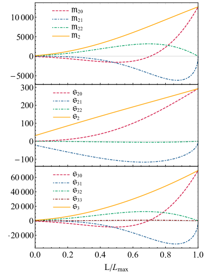
Figure 1: The quantities $\mathfrak{M}_{2}$ (top panel), $\mathfrak{S}_{2}$ (middle panel), and $\mathfrak{S}_{3}$ (bottom panel) defined in Eq. (3.27) and the normalized components of the corresponding moments for a representative choice of $\kappa_{i}=(325,751,798,272)$ (corresponding to $L_{\rm max}=79.3361$) as a function of $L/L_{\rm max}\leq 1$. In the top and bottom panels the horizontal thin black line refers to the fuzzball and Kerr moments being identical, whereas $\mathfrak{S}_{2m}$ are identically zero for Kerr. All quantities are larger than their Kerr counterpart when $L\sim L_{\rm max}$ while in this example some can be smaller when $L\ll L_{\rm max}$. In the $L\to 0$ limit the normalized quantities tend to some small but nonvanishing values.

To gain some further insight and check these trends, we apply the method presented in the previous sections to compute the multipole moments of general solutions found by randomly selecting the parameters $L$ and $\kappa_{i}$ (with $i=1,2,3,4$). In particular, we draw $10^{4}$ realizations from a uniform distribution

$$\kappa_{i}\in[1,\kappa_{\rm max}]\,,$$ (3.67)

constrained by imposing that the conditions in Eq. (3.32) be satisfied. As a representative case we choose $\kappa_{\rm max}=1000$. For a given choice of $\kappa_{i}$, we draw $L$ from a uniform distribution

$$L\in(0,L_{\rm max}]\,,$$ (3.68)

where $L_{\rm max}$ is given in (3.43), or is chosen to be $L_{\rm max}=10^{4}$ for those (few) isolated cases in which $L$ is unbounded.

We find two main results:

1. The normalized invariant $\mathfrak{M}_{2}$ defined in (3.27) is bigger than its Kerr value ($\mathfrak{M}_{2}^{\rm Kerr}=1$) for about $90\%$ of the solutions. Similar (slightly higher) percentages apply also to higher-order moments and, in particular, to $\mathfrak{S}_{3}$. These percentages do not depend on the choice of $\kappa_{\rm max}$, suggesting that both $L_{\rm crit}$ and $L_{\rm max}$ grow linearly with $\kappa_{i}\gg 1$.

2. For each random realization of $\kappa_{i}$, the normalized invariants $\mathfrak{M}_{\ell}$ and $\mathfrak{S}_{\ell}$ are always bigger than their value in the (non-rotating) BH limit, i.e. when $L\to 0$, even when the corresponding moments are not defined in that limit Bena:2020see ; Bena:2020uup . Indeed, we numerically find that these quantities are always monotonous functions of $L$, attaining a global minimum at $L=0$. Note that this property holds only for the specific invariants defined by a specific combination of the components of each moment (e.g., Eq. (3.27), see also Appendix A) and not for the individual components of the moments (e.g., $\mathfrak{M}_{\ell 0}$ and $\mathfrak{S}_{\ell 0}$ as defined in Eq. (3.26)).

4 Conclusions and discussion

We have extended and refined a general method to determine the multipole moments of spacetimes with a single timelike Killing vector field and no extra symmetry. In particular, this technique is useful in the study of the moments of fuzzball microstate geometries. These typically break the axial and equatorial symmetries the Kerr metric and are also rather complicated. We focused on three-center solutions, but our analysis can be straightforwardly applied to generic multi-center solutions and generic BH solutions.

The multipolar structure of fuzzballs is significantly richer than that of a BH in GR, in particular multipole moments ${\cal M}_{\ell m}$ and ${\cal S}_{\ell m}$ with $m\neq 0$ (associated with the absence of axial and equatorial symmetry) are non-zero, at variance with the Kerr metric Bianchi:2020bxa .

All astrophysical observations so far are perfectly consistent with the hypothesis that all dark compact objects in the universe can be described by the Kerr metric Cardoso:2019rvt . Thus, from a phenomenological point of view an interesting problem is to understand whether current and future observations can distinguish the classical Kerr metric from other paradigms, such as the fuzzball proposal. Here we compared the multipole moments of a large family of smooth horizonless geometries with those of a BH with the same mass and spin.

Another natural question would be to compare the multipolar structure of individual microstates with the one of the corresponding BH that should emerge from their ensemble. Unfortunately, to the best of our knowledge no fuzzball solutions in four dimensions are known beyond the BPS case, and supersymmetric BHs are necessarily non-spinning in four dimensions Townsend:2002yf . Still, a comparison between the individual microstate and its Schwarzschild (or Reissner-Nordström) BH limit can be performed for some dimensionless ratios which are finite in the BH limit. The universal properties of these ratios in the context of BH microstates has been recently studied in Bena:2020see ; Bena:2020uup . We find strong numerical evidence that these ratios grow monotonically with the microstate size $L$, attaining a minimum at the BH limit, $L\to 0$. A similar study has been performed in the past for exotic compact objects (e.g., gravastars and anisotropic stars) Yagi:2015upa ; Pani:2015tga ; Uchikata:2015yma ; Uchikata:2016qku ; Raposo:2018xkf suggesting the universal character of this property. We also find that the maximum size $L_{\rm max}$ is always smaller than the horizon length scale $r_{H}\sim(Q_{1}Q_{2}Q_{3}P_{0})^{1/4}$, and that $L_{\rm max}\ll r_{H}$ for large charges. In this limit the dimensionless spin $\chi={\cal J}/{\cal M}^{2}$ is always small, consistently with the fact the solutions represent microstates of a non-rotating BH.

Although the study of the multipole moments of microstate geometries has just started Bena:2020see ; Bianchi:2020bxa ; Bena:2020uup and can be extended in various directions, some intriguing generic properties seem to appear, such as the fact that the BH metric seems to be the solution with a given mass and spin that typically minimizes the multipole moments or certain combinations thereof. Indeed, we found that the invariant built from the dimensionless multipole moments of the Kerr metric are smaller than those of a given microstate with the same mass and spin in approximately $90\%$ of the four-dimensional parameter space of three-center solutions.

It is also intriguing to note that the Lyapunov exponent of unstable null geodesics near the photon sphere was found to be maximum for the BH solution relative to the microstate geometries Bianchi:2020des . This suggests that the BH metric is an extremum in the parameter space of the solutions of the theory for several (apparently disconnected) quantities.

Clearly, some interesting extensions of our work are to find an analytical proof of the monotonous behaviour of $\mathfrak{M}_{\ell}$ and $\mathfrak{S}_{\ell}$, and to check whether the above properties hold true also for other multi-center microstate geometries.

We stress the fact that our method can be directly applied to non-BPS microstate solutions when such solutions would be available. In this case microstate geometries with $\chi={\cal O}(1)$ should exist. Such an analysis might help understanding how the multipole moments of a classical BH could emerge from an averaging of an ensemble of microstates, each microstate having a different multipolar structure.

There is a long way to go before observationally imprints of fuzzballs in astrophysical systems can be modelled accurately and, in this respect, several interesting extensions of this and recent studies Bena:2020see ; Bianchi:2020bxa ; Bena:2020uup are urgent. Nonetheless, we believe that the analysis of the multipole moments can provide a new portal to constrain fuzzball models with current and future observations, by means of both electromagnetic and gravitational-wave probes.

Note added. While this work was in preparation, a related work by Iosif Bena and Daniel R. Mayerson appeared Bena:2020uup . Ref. Bena:2020uup and our work are the longer companions to Refs. Bena:2020see and Bianchi:2020bxa , respectively.

Appendix A Invariants associated to multipole moments

Using the Cartesian description of the multipoles we can construct some quantities which are invariant under rotations. We start from the general formula which connects the Cartesian and the spherical descriptions,

$${1\over\ell!}{\cal Q}^{i_{1}\dots i_{\ell}}n_{i_{1}}\dots n_{i_{\ell}}=\sqrt{4\pi\over 2\ell+1}\sum_{m=-\ell}^{+\ell}\mathcal{M}_{\ell m}Y_{\ell m}$$ (A.1)

where ${\cal Q}^{i_{1}\dots i_{\ell}}$ is a symmetric traceless tensor. We now specialize our computation to the cases $\ell=1,2,3$ ($\ell=0$ is trivial).

Dipole moments.

For $\ell=1$, ${\cal Q}_{1}^{i}$ is a vector. Using (A.1) we can write the components of ${\cal Q}^{i}$ in terms of ${\cal M}_{1m}$:

$${\cal Q}_{1}^{x}=\sqrt{2}({\cal M}_{1-1}-{\cal M}_{11})\quad,\quad{\cal Q}_{1}^{y}=-i\sqrt{2}({\cal M}_{1-1}+{\cal M}_{11})\quad,\quad{\cal Q}_{1}^{z}=2{\cal M}_{10}\,.$$ (A.2)

The only invariant associated to ${\cal Q}_{1}^{i}$ is

$$\frac{1}{4}|\vec{Q}_{1}|^{2}=\frac{1}{4}Q_{1}^{i}Q_{1,i}={\cal M}_{10}^{2}+2|{\cal M}_{11}|^{2}$$ (A.3)

Quadrupole moments.

For $\ell=2$, ${\cal Q}_{2}^{ij}$ is a symmetric traceless matrix, therefore there are 5 (real) independent components. In terms of the ${\cal M}_{2m}$ we have

$$\begin{aligned} \mathcal{Q}_{2}^{xx}&=\sqrt{\frac{3}{2}}({\cal M}_{22}+{\cal M}_{2-2})-{\cal M}_{20}\quad,\quad\mathcal{Q}_{2}^{yy}=-\sqrt{\frac{3}{2}}({\cal M}_{22}+{\cal M}_{2-2})-{\cal M}_{20}\\ \mathcal{Q}_{2}^{xy}&=i\sqrt{\frac{3}{2}}({\cal M}_{22}{-}{\cal M}_{2-2})\quad,\quad\mathcal{Q}_{2}^{xz}=\sqrt{\frac{3}{2}}({\cal M}_{2-1}{-}{\cal M}_{21})\quad,\quad\mathcal{Q}_{2}^{yz}=-i\sqrt{\frac{3}{2}}({\cal M}_{2-1}{+}{\cal M}_{21})\\ \mathcal{Q}_{2}^{zz}&=-\mathcal{Q}_{2}^{xx}-\mathcal{Q}_{2}^{yy}=2{\cal M}_{20}\end{aligned}\,.$$ (A.4)

We can associate two invariants to the $\mathcal{Q}$ matrix, namely its trace and determinant. In terms of ${\cal M}_{2m}$ they read

$$\begin{aligned} \frac{1}{6}\text{Tr}{\cal Q}^{2}&={\cal M}_{20}^{2}+2|{\cal M}_{22}|^{2}+2|{\cal M}_{21}|^{2}\\ \frac{1}{2}\text{Det}{\cal Q}&={\cal M}_{20}^{3}+3{\cal M}_{20}(|{\cal M}_{21}|^{2}-2|{\cal M}_{22}|^{2})+3\sqrt{6}\,\text{Re}[{\cal M}_{22}^{*}{\cal M}_{21}^{2}]\end{aligned}\,.$$ (A.5)

Octupole moments.

In a similar fashion one can compute the trace invariant associated to ${\cal Q}_{3}$, which is defined as

$${1\over 3!}{\cal Q}_{3}^{ijk}n_{i}n_{j}n_{k}=\sqrt{4\pi\over 7}\sum_{m=-3}^{+3}{\cal M}_{3m}Y_{3m}\,.$$ (A.6)

The octupole tensor ${\cal Q}_{3}^{ijk}$ has 7 independent components. The relations with the ${\cal M}_{3m}$ are the following

$$\begin{aligned} \mathcal{Q}_{3}^{xxx}&=\frac{3}{2}(\sqrt{5}{\cal M}_{3-3}-\sqrt{3}{\cal M}_{3-1}+\sqrt{3}{\cal M}_{31}-\sqrt{5}{\cal M}_{3,3})\\ \mathcal{Q}_{3}^{xxy}&=-\frac{i}{2}(3\sqrt{5}{\cal M}_{3-3}-\sqrt{3}{\cal M}_{3-1}-\sqrt{3}{\cal M}_{31}+3\sqrt{5}{\cal M}_{3,3})\\ \mathcal{Q}_{3}^{xxz}&=\frac{1}{2}(\sqrt{30}{\cal M}_{3-2}-6{\cal M}_{30}+\sqrt{30}{\cal M}_{32})\\ \mathcal{Q}_{3}^{xyy}&=\frac{1}{2}(-3\sqrt{5}{\cal M}_{3-3}-\sqrt{3}{\cal M}_{3-1}+\sqrt{3}{\cal M}_{31}+3\sqrt{5}{\cal M}_{3,3})\\ \mathcal{Q}_{3}^{xyz}&=-i\sqrt{\frac{15}{2}}({\cal M}_{3-2}-{\cal M}_{32})\\ \mathcal{Q}_{3}^{yyy}&=\frac{3i}{2}(\sqrt{5}{\cal M}_{3-3}+\sqrt{3}{\cal M}_{3-1}+\sqrt{3}{\cal M}_{31}+\sqrt{5}{\cal M}_{3,3})\\ \mathcal{Q}_{3}^{yyz}&=-\frac{1}{2}(\sqrt{30}{\cal M}_{3-2}+6{\cal M}_{30}+\sqrt{30}{\cal M}_{32})\\ \mathcal{Q}_{3}^{xzz}&=-\mathcal{Q}_{3}^{xxx}-\mathcal{Q}_{3}^{xyy}=2\sqrt{3}\left({\cal M}_{3-1}-{\cal M}_{31}\right)\\ \mathcal{Q}_{3}^{yzz}&=-\mathcal{Q}_{3}^{xxy}-\mathcal{Q}_{3}^{yyy}=-2i\sqrt{3}\left({\cal M}_{3-1}+{\cal M}_{31}\right)\\ \mathcal{Q}_{3}^{zzz}&=-\mathcal{Q}_{3}^{xxz}-\mathcal{Q}_{3}^{yyz}=6{\cal M}_{30}\end{aligned}\,.$$ (A.7)

We can compute $\text{Tr}{\cal Q}_{3}^{2}={\cal Q}_{3}^{ijk}{\cal Q}_{3,\,ijk}$ obtaining

$$\frac{1}{90}\text{Tr}{\cal Q}_{3}^{2}={\cal M}_{30}^{2}+2|{\cal M}_{33}|^{2}+2|{\cal M}_{32}|^{2}+2|{\cal M}_{31}|^{2}\,.$$ (A.8)

Appendix B Multipole moments of general classes of microstate geometries

In this appendix we provide the multipole moments for some generic class of solutions. As discussed in the main text the parameter $L$ is generically bounded, $L\leq L_{\rm max}$, except for some particular solutions. Since in the large-$\kappa$ limit typically $L_{\rm max}={\cal O}(\kappa)$, we shall distinguish between two opposite regimes:

1. $L$ is much smaller than the leading parameter(s) $\kappa_{i}$ (this includes the small-$L$ limit);

2. $L\sim L_{\rm max}={\cal O}(\kappa)$.

B.1 General solution with $\kappa_{1}={\cal O}(1)$, $\kappa_{2}=0$, $\kappa_{3}={\cal O}(1)$, $\kappa_{4}\gg 1$

We consider the case in which $\kappa_{2}=0$, $\kappa_{1,3}\sim{\cal O}(1)$ and $\kappa_{4}\gg\kappa_{1,3}$. To simplify the notation we define $(\kappa_{1},\kappa_{3},\kappa_{4})=(\bar{\kappa}_{1},\bar{\kappa}_{3},\bar{\kappa}_{4}\lambda)$, where $\bar{\kappa_{i}}\sim{\cal O}(1)$ and $\lambda\gg 1$.

B.1.1 Small $L$

If $L\ll\lambda$, to leading order in $\lambda$ the centers are located at

$$\textbf{x}_{1} =\left(-\frac{\left(\bar{\kappa}_{1}^{2}\bar{\kappa}_{3}^{2}-2\bar{\kappa}_{1}\bar{\kappa}_{3}^{2}-1\right)L\sqrt{3\bar{\kappa}_{1}^{2}\bar{\kappa}_{3}^{4}+L^{2}+4\bar{\kappa}_{1}\bar{\kappa}_{3}^{2}L}}{\left(\bar{\kappa}_{1}+1\right)\bar{\kappa}_{3}\bar{\kappa}_{4}\lambda\left(2\bar{\kappa}_{1}\bar{\kappa}_{3}^{2}+L\right)},0,\frac{2\bar{\kappa}_{1}^{2}\bar{\kappa}_{3}^{2}L}{\left(\bar{\kappa}_{1}+1\right)\left(2\bar{\kappa}_{1}\bar{\kappa}_{3}^{2}+L\right)}\right),$$ (B.1)

$$\textbf{x}_{2} =\left(\frac{\left(\left(2\bar{\kappa}_{1}-1\right)\bar{\kappa}_{3}^{2}+1\right)L\sqrt{3\bar{\kappa}_{1}^{2}\bar{\kappa}_{3}^{4}+L^{2}+4\bar{\kappa}_{1}\bar{\kappa}_{3}^{2}L}}{\left(\bar{\kappa}_{1}+1\right)\bar{\kappa}_{3}\bar{\kappa}_{4}\lambda\left(2\bar{\kappa}_{1}\bar{\kappa}_{3}^{2}+L\right)},0,-\frac{2\bar{\kappa}_{1}\bar{\kappa}_{3}^{2}L}{\left(\bar{\kappa}_{1}+1\right)\left(2\bar{\kappa}_{1}\bar{\kappa}_{3}^{2}+L\right)}\right),$$ (B.2)

$$\textbf{x}_{3} =\left(-\frac{L\sqrt{3\bar{\kappa}_{1}^{2}\bar{\kappa}_{3}^{4}+L^{2}+4\bar{\kappa}_{1}\bar{\kappa}_{3}^{2}L}}{2\bar{\kappa}_{1}\bar{\kappa}_{3}^{2}+L},0,\frac{\left(\bar{\kappa}_{1}-1\right)\bar{\kappa}_{1}\bar{\kappa}_{3}^{2}L}{\left(\bar{\kappa}_{1}+1\right)\left(2\bar{\kappa}_{1}\bar{\kappa}_{3}^{2}+L\right)}\right),$$ (B.3)

and the first multipole moments of this solution read

$$\mathcal{M}_{00} =\frac{1}{4}\lambda\left(\bar{\kappa}_{1}+1\right)\bar{\kappa}_{3}\bar{\kappa}_{4}\quad,\quad\mathcal{S}_{10}=\frac{\lambda L\bar{\kappa}_{1}\bar{\kappa}_{3}^{2}\bar{\kappa}_{4}}{4\bar{\kappa}_{1}\bar{\kappa}_{3}^{2}+2L}\,,$$ (B.4)

$$\mathcal{M}_{22} ={\cal O}\left(\lambda^{0}\right)\,,\qquad\mathcal{M}_{21}={\cal O}\left(\lambda^{0}\right)\,,\qquad\mathcal{M}_{20}=\frac{\lambda L^{2}\bar{\kappa}_{1}^{3}\bar{\kappa}_{3}^{5}\bar{\kappa}_{4}}{\left(\bar{\kappa}_{1}+1\right)\left(2\bar{\kappa}_{1}\bar{\kappa}_{3}^{2}+L\right){}^{2}}\,,$$

$$\mathcal{S}_{22} ={\cal O}\left(\lambda^{0}\right)\,,\qquad\mathcal{S}_{21}={\cal O}\left(\lambda^{0}\right)\,,\qquad\mathcal{S}_{20}=\frac{\lambda L^{2}\left(\bar{\kappa}_{1}-1\right)\bar{\kappa}_{1}^{2}\bar{\kappa}_{3}^{4}\bar{\kappa}_{4}}{\left(\bar{\kappa}_{1}+1\right)\left(2\bar{\kappa}_{1}\bar{\kappa}_{3}^{2}+L\right){}^{2}}\,.$$

B.2 General solution with $\kappa_{1}={\cal O}(1)$, $\kappa_{2}=0$, and $\kappa_{3,4}\gg 1$

Here we consider the solution for which $\kappa_{2}=0$ and $\kappa_{3,4}\gg\kappa_{1}$. We define $(\kappa_{1},\kappa_{3},\kappa_{4})=(\bar{\kappa}_{1},\bar{\kappa}_{3}\lambda,\bar{\kappa}_{4}\lambda)$, where $\bar{\kappa_{i}}\sim{\cal O}(1)$ and $\lambda\gg 1$.

B.2.1 Small $L$

If $L\ll\lambda$, to leading order in the expansion for large $\lambda$, the coordinates of the centers are

$$\textbf{x}_{1} =\frac{1}{{\cal A}}\left(-\left(\sqrt{3}\bar{\kappa}_{1}\bar{\kappa}_{3}\left(\bar{\kappa}_{1}\left(\bar{\kappa}_{3}+\bar{\kappa}_{4}\right)-2\bar{\kappa}_{4}\right)\right),0,-\bar{\kappa}_{1}\left(\left(\bar{\kappa}_{1}-2\right)\bar{\kappa}_{3}-2\bar{\kappa}_{4}\right)\left(\bar{\kappa}_{3}-\bar{\kappa}_{4}\right)\right),$$ (B.5)

$$\textbf{x}_{2} =\frac{1}{{\cal A}}\left(-\sqrt{3}\bar{\kappa}_{3}\left(\bar{\kappa}_{4}+\bar{\kappa}_{1}\left(\bar{\kappa}_{3}-2\bar{\kappa}_{4}\right)\right),0,-2\bar{\kappa}_{1}^{2}\bar{\kappa}_{3}^{2}+\bar{\kappa}_{1}\bar{\kappa}_{3}^{2}+\bar{\kappa}_{4}\left(2\bar{\kappa}_{4}-\bar{\kappa}_{3}\right)\right),$$ (B.6)

$$\textbf{x}_{3} =\frac{1}{{\cal A}}\left(-\sqrt{3}\bar{\kappa}_{4}\left(\bar{\kappa}_{4}+\bar{\kappa}_{1}\left(\bar{\kappa}_{4}-2\bar{\kappa}_{3}\right)\right),0,\left(\bar{\kappa}_{1}-1\right)\left(2\left(\bar{\kappa}_{1}+1\right)\bar{\kappa}_{3}-\bar{\kappa}_{4}\right)\bar{\kappa}_{4}\right),$$ (B.7)

where the denominator is ${\cal A}=2\left(\bar{\kappa}_{4}+\bar{\kappa}_{1}\left(\bar{\kappa}_{3}+\bar{\kappa}_{4}\right)\right)\sqrt{\left(\bar{\kappa}_{1}^{2}-\bar{\kappa}_{1}+1\right)\bar{\kappa}_{3}^{2}-\left(\bar{\kappa}_{1}+1\right)\bar{\kappa}_{4}\bar{\kappa}_{3}+\bar{\kappa}_{4}^{2}}$. Note that the square root in ${\cal A}$ is proportional to the angular momentum, which implies that the zero angular momentum limit is singular. Indeed, this general solution does not include Solution A in the main text. The latter (as well as all solutions in this class for which $\mathbfcal{J}=0$) must be studied separately.

To leading order in $\lambda$, the first multipole moments of this solution read

$$\mathcal{M}_{00} =\frac{1}{4}\lambda^{2}\bar{\kappa}_{3}\left(\bar{\kappa}_{4}+\bar{\kappa}_{1}\left(\bar{\kappa}_{3}+\bar{\kappa}_{4}\right)\right)\quad,\quad\mathcal{S}_{10}=\frac{1}{4}\lambda L\sqrt{\left(\bar{\kappa}_{1}^{2}-\bar{\kappa}_{1}+1\right)\bar{\kappa}_{3}^{2}-\left(\bar{\kappa}_{1}+1\right)\bar{\kappa}_{4}\bar{\kappa}_{3}+\bar{\kappa}_{4}^{2}}\,,$$ (B.8)

$$\mathcal{M}_{22} =\frac{\lambda^{2}L^{2}}{{\cal A}^{2}}\frac{3}{8}\sqrt{\frac{3}{2}}\bar{\kappa}_{1}\bar{\kappa}_{3}^{2}\bar{\kappa}_{4}\left(\bar{\kappa}_{4}+\bar{\kappa}_{1}\left(\bar{\kappa}_{3}+\bar{\kappa}_{4}\right)\right)\left(\bar{\kappa}_{3}\left(\bar{\kappa}_{3}+\bar{\kappa}_{4}\right)\bar{\kappa}_{1}^{2}+\left(\bar{\kappa}_{3}^{2}-6\bar{\kappa}_{4}\bar{\kappa}_{3}+\bar{\kappa}_{4}^{2}\right)\bar{\kappa}_{1}+\bar{\kappa}_{4}\left(\bar{\kappa}_{3}+\bar{\kappa}_{4}\right)\right)\,,$$

$$\mathcal{M}_{21} =\frac{\lambda^{2}L^{2}}{{\cal A}^{2}}\frac{9}{4\sqrt{2}}\left(\bar{\kappa}_{1}-1\right)\bar{\kappa}_{1}\bar{\kappa}_{3}^{2}\left(\bar{\kappa}_{3}-\bar{\kappa}_{4}\right)\left(\bar{\kappa}_{1}\bar{\kappa}_{3}-\bar{\kappa}_{4}\right)\bar{\kappa}_{4}\left(\bar{\kappa}_{4}+\bar{\kappa}_{1}\left(\bar{\kappa}_{3}+\bar{\kappa}_{4}\right)\right)\,,$$

$$\mathcal{M}_{20} =\frac{\lambda^{2}L^{2}}{{\cal A}^{2}}\frac{1}{8}\bar{\kappa}_{1}\bar{\kappa}_{3}\bar{\kappa}_{4}\left(\left(8\bar{\kappa}_{1}^{3}-9\bar{\kappa}_{1}^{2}-9\bar{\kappa}_{1}+8\right)\bar{\kappa}_{3}^{3}-3\left(3\bar{\kappa}_{1}^{2}-10\bar{\kappa}_{1}+3\right)\bar{\kappa}_{4}\bar{\kappa}_{3}^{2}-9\left(\bar{\kappa}_{1}+1\right)\bar{\kappa}_{4}^{2}\bar{\kappa}_{3}\right.$$

$$\left.+8\bar{\kappa}_{4}^{3}\right)\left(\bar{\kappa}_{4}+\bar{\kappa}_{1}\left(\bar{\kappa}_{3}+\bar{\kappa}_{4}\right)\right)\,,$$

$$\mathcal{S}_{22} =-\frac{\lambda L^{2}}{{\cal A}^{2}}\frac{3}{8}\sqrt{\frac{3}{2}}\left(\bar{\kappa}_{1}-1\right)\bar{\kappa}_{3}\left(\bar{\kappa}_{3}-\bar{\kappa}_{4}\right)\left(\bar{\kappa}_{1}\bar{\kappa}_{3}-\bar{\kappa}_{4}\right)\left(\bar{\kappa}_{4}+\bar{\kappa}_{1}\left(\bar{\kappa}_{3}+\bar{\kappa}_{4}\right)\right){}^{2}\,,$$

$$\mathcal{S}_{21} =\frac{\lambda L^{2}}{{\cal A}^{2}}\frac{3}{4\sqrt{2}}\bar{\kappa}_{3}\left(\bar{\kappa}_{4}+\bar{\kappa}_{1}\left(\bar{\kappa}_{3}+\bar{\kappa}_{4}\right)\right)\left(\bar{\kappa}_{3}\left(\bar{\kappa}_{3}^{2}-4\bar{\kappa}_{4}\bar{\kappa}_{3}+\bar{\kappa}_{4}^{2}\right)\bar{\kappa}_{1}^{3}+\left(\bar{\kappa}_{3}^{3}+2\bar{\kappa}_{4}\bar{\kappa}_{3}^{2}+2\bar{\kappa}_{4}^{2}\bar{\kappa}_{3}+\bar{\kappa}_{4}^{3}\right)\bar{\kappa}_{1}^{2}\right.$$

$$\left.+2\bar{\kappa}_{4}\left(-2\bar{\kappa}_{3}^{2}+\bar{\kappa}_{4}\bar{\kappa}_{3}-2\bar{\kappa}_{4}^{2}\right)\bar{\kappa}_{1}+\bar{\kappa}_{4}^{2}\left(\bar{\kappa}_{3}+\bar{\kappa}_{4}\right)\right)\,,$$

$$\mathcal{S}_{20} =\frac{\lambda L^{2}}{{\cal A}^{2}}\frac{1}{8}\left(\bar{\kappa}_{4}+\bar{\kappa}_{1}\left(\bar{\kappa}_{3}+\bar{\kappa}_{4}\right)\right)\left(8\bar{\kappa}_{3}^{3}\left(\bar{\kappa}_{3}-\bar{\kappa}_{4}\right)\bar{\kappa}_{1}^{4}-7\left(\bar{\kappa}_{3}^{4}-\bar{\kappa}_{3}^{2}\bar{\kappa}_{4}^{2}\right)\bar{\kappa}_{1}^{3}+7\left(\bar{\kappa}_{3}^{4}-\bar{\kappa}_{3}\bar{\kappa}_{4}^{3}\right)\bar{\kappa}_{1}^{2}\right.$$

$$\left.-8\left(\bar{\kappa}_{3}^{4}-\bar{\kappa}_{4}^{4}\right)\bar{\kappa}_{1}+\bar{\kappa}_{4}\left(8\bar{\kappa}_{3}^{3}-7\bar{\kappa}_{4}\bar{\kappa}_{3}^{2}+7\bar{\kappa}_{4}^{2}\bar{\kappa}_{3}-8\bar{\kappa}_{4}^{3}\right)\right)\,,$$

Notice that in the denominator of each of the multipoles there is a term proportional to the angular momentum.

B.3 General solution with $\kappa_{1}={\cal O}(1)$ and $\kappa_{2,3,4}\gg 1$

An even more general solution with $\kappa_{2}\neq 0$ can be constructed analytically when $(\kappa_{1},\kappa_{2},\kappa_{3},\kappa_{4})=(\bar{\kappa}_{1},\bar{\kappa}_{2}\lambda,\bar{\kappa}_{3}\lambda,\bar{\kappa}_{4}\lambda)$, where $\bar{\kappa_{i}}\sim{\cal O}(1)$ and $\lambda\gg 1$.

B.3.1 Small $L$

If $L\ll\lambda$, to leading order in $\lambda\gg 1$ the first multipole moments of this class of solutions are

$$\mathcal{M}_{00} =\frac{1}{4}\lambda^{2}\left(\bar{\kappa}_{1}\bar{\kappa}_{2}^{2}+4\bar{\kappa}_{1}\bar{\kappa}_{3}\bar{\kappa}_{2}-\bar{\kappa}_{1}\bar{\kappa}_{4}\bar{\kappa}_{2}-\bar{\kappa}_{4}\bar{\kappa}_{2}+\bar{\kappa}_{1}\bar{\kappa}_{3}^{2}+\bar{\kappa}_{1}\bar{\kappa}_{3}\bar{\kappa}_{4}+\bar{\kappa}_{3}\bar{\kappa}_{4}\right)\,,$$ (B.9)

$$\mathcal{S}_{10} =\frac{\lambda^{3}L\bar{\kappa}_{1}\bar{\kappa}_{2}\left(\bar{\kappa}_{2}-\bar{\kappa}_{3}\right){}^{2}\bar{\kappa}_{3}\bar{\kappa}_{4}}{4\bar{\kappa}_{2}^{2}+4\bar{\kappa}_{3}^{2}+2(L+5)\bar{\kappa}_{3}\bar{\kappa}_{2}}\,,$$

$$\mathcal{M}_{22} =\frac{\lambda^{2}L^{2}}{\cal Z}\sqrt{\frac{3}{2}}\bar{\kappa}_{1}\left(\bar{\kappa}_{2}+\bar{\kappa}_{3}\right){}^{2}\left(\left(\bar{\kappa}_{3}-\bar{\kappa}_{2}\right)\bar{\kappa}_{4}+\bar{\kappa}_{1}\left(\bar{\kappa}_{2}\left(2\bar{\kappa}_{3}-\bar{\kappa}_{4}\right)+\bar{\kappa}_{3}\bar{\kappa}_{4}\right)\right)\left(3\bar{\kappa}_{2}^{4}+3\bar{\kappa}_{3}^{4}\right.$$

$$\left.+\left(L^{2}+10L+27\right)\bar{\kappa}_{3}^{2}\bar{\kappa}_{2}^{2}+4(L+6)\bar{\kappa}_{3}\bar{\kappa}_{2}^{3}+4(L+6)\bar{\kappa}_{3}^{3}\bar{\kappa}_{2}\right)\,,$$

$$\mathcal{M}_{21} =-\frac{\lambda^{2}L^{2}}{\cal Z}\sqrt{6}\left(\bar{\kappa}_{1}-1\right)\bar{\kappa}_{1}\left(\bar{\kappa}_{2}-\bar{\kappa}_{3}\right){}^{2}\left(\bar{\kappa}_{2}+\bar{\kappa}_{3}\right){}^{3}\bar{\kappa}_{4}\left(3\bar{\kappa}_{2}^{4}+3\bar{\kappa}_{3}^{4}+\left(L^{2}+10L+27\right)\bar{\kappa}_{3}^{2}\bar{\kappa}_{2}^{2}\right.$$

$$\left.+4(L+6)\bar{\kappa}_{3}\bar{\kappa}_{2}^{3}+4(L+6)\bar{\kappa}_{3}^{3}\bar{\kappa}_{2}\right)^{1/2}\,,$$

$$\mathcal{M}_{20} =-\frac{\lambda^{2}\-L^{2}}{{\cal Z}}\left[8\bar{\kappa}_{2}\bar{\kappa}_{3}\bar{\kappa}_{4}^{2}\left(\bar{\kappa}_{2}-\bar{\kappa}_{3}\right){}^{4}-\bar{\kappa}_{1}\bar{\kappa}_{4}\left(\bar{\kappa}_{2}-\bar{\kappa}_{3}\right)\left(\bar{\kappa}_{2}^{6}+\bar{\kappa}_{3}^{5}\left(\bar{\kappa}_{3}-8\bar{\kappa}_{4}\right)\right.\right.$$

$$+\bar{\kappa}_{3}\bar{\kappa}_{2}^{4}\left(\left(L^{2}+18L+112\right)\bar{\kappa}_{3}-24\bar{\kappa}_{4}\right)+2\bar{\kappa}_{3}^{2}\bar{\kappa}_{2}^{3}\left(16\bar{\kappa}_{4}+\left(L^{2}+14L+23\right)\bar{\kappa}_{3}\right)$$

$$\left.+\bar{\kappa}_{3}^{3}\bar{\kappa}_{2}^{2}\left(\left(L^{2}+18L+112\right)\bar{\kappa}_{3}-32\bar{\kappa}_{4}\right)+\bar{\kappa}_{2}^{5}\left(8\bar{\kappa}_{4}+(4L+26)\bar{\kappa}_{3}\right)+2\bar{\kappa}_{3}^{4}\bar{\kappa}_{2}\left(12\bar{\kappa}_{4}+(2L+13)\bar{\kappa}_{3}\right)\right)$$

$$+\bar{\kappa}_{1}^{2}\left(\left(2\bar{\kappa}_{3}-\bar{\kappa}_{4}\right)\bar{\kappa}_{2}^{7}+\bar{\kappa}_{3}^{7}\bar{\kappa}_{4}+\bar{\kappa}_{3}\bar{\kappa}_{2}^{5}\left(8\bar{\kappa}_{4}^{2}+2\left(L^{2}+18L+96\right)\bar{\kappa}_{3}^{2}-\left(L^{2}+14L+86\right)\bar{\kappa}_{4}\bar{\kappa}_{3}\right)\right.$$

$$+\bar{\kappa}_{3}^{2}\bar{\kappa}_{2}^{4}\left(-32\bar{\kappa}_{4}^{2}+4\left(L^{2}+14L+35\right)\bar{\kappa}_{3}^{2}-\left(L^{2}+10L-66\right)\bar{\kappa}_{4}\bar{\kappa}_{3}\right)+\bar{\kappa}_{3}^{3}\bar{\kappa}_{2}^{3}\left(48\bar{\kappa}_{4}^{2}\right.$$

$$\left.+2\left(L^{2}+18L+96\right)\bar{\kappa}_{3}^{2}+\left(L^{2}+10L-66\right)\bar{\kappa}_{4}\bar{\kappa}_{3}\right)+\bar{\kappa}_{3}^{4}\bar{\kappa}_{2}^{2}\left(-32\bar{\kappa}_{4}^{2}+\left(L^{2}+14L+86\right)\bar{\kappa}_{4}\bar{\kappa}_{3}\right.$$

$$\left.\left.\left.+(8L+60)\bar{\kappa}_{3}^{2}\right)+\bar{\kappa}_{3}\bar{\kappa}_{2}^{6}\left((8L+60)\bar{\kappa}_{3}-(4L+25)\bar{\kappa}_{4}\right)+\bar{\kappa}_{3}^{5}\bar{\kappa}_{2}\left(2\bar{\kappa}_{3}^{2}+8\bar{\kappa}_{4}^{2}+(4L+25)\bar{\kappa}_{4}\bar{\kappa}_{3}\right)\right)\right]\,,$$

$$\mathcal{S}_{22} =0\,,$$

$$\mathcal{S}_{21} =\frac{\lambda^{3}L^{2}}{\cal Z}2\sqrt{6}\bar{\kappa}_{1}^{2}\bar{\kappa}_{2}\left(\bar{\kappa}_{2}-\bar{\kappa}_{3}\right){}^{2}\bar{\kappa}_{3}\left(\bar{\kappa}_{2}+\bar{\kappa}_{3}\right){}^{2}\bar{\kappa}_{4}\left(3\bar{\kappa}_{2}^{4}+3\bar{\kappa}_{3}^{4}+\left(L^{2}+10L+27\right)\bar{\kappa}_{3}^{2}\bar{\kappa}_{2}^{2}\right.$$

$$\left.+4(L+6)\bar{\kappa}_{3}\bar{\kappa}_{2}^{3}+4(L+6)\bar{\kappa}_{3}^{3}\bar{\kappa}_{2}\right)^{1/2}\,,$$

$$\mathcal{S}_{20} =\frac{\lambda^{3}L^{2}}{\cal Z}8\left(\bar{\kappa}_{1}-1\right)\bar{\kappa}_{1}\bar{\kappa}_{2}\left(\bar{\kappa}_{2}-\bar{\kappa}_{3}\right){}^{4}\bar{\kappa}_{3}\left(\bar{\kappa}_{2}+\bar{\kappa}_{3}\right)\bar{\kappa}_{4}^{2}\,.$$

where for readability we have defined

$${\cal Z}=8\left(\left(\bar{\kappa}_{3}-\bar{\kappa}_{2}\right)\bar{\kappa}_{4}+\bar{\kappa}_{1}\left(\bar{\kappa}_{2}^{2}+\left(4\bar{\kappa}_{3}-\bar{\kappa}_{4}\right)\bar{\kappa}_{2}+\bar{\kappa}_{3}\left(\bar{\kappa}_{3}+\bar{\kappa}_{4}\right)\right)\right)\left(2\bar{\kappa}_{2}^{2}+2\bar{\kappa}_{3}^{2}+(L+5)\bar{\kappa}_{3}\bar{\kappa}_{2}\right){}^{2}\,.$$ (B.10)

B.3.2 $L\sim L_{\rm max}$

Since $L\sim L_{\rm max}\sim\lambda$, we can define $L=\bar{L}\lambda$ and, to leading order in $\lambda$, the multipole moments read

$$\mathcal{M}_{00} =\frac{1}{4}\lambda^{2}\left(\left(\bar{\kappa}_{3}-\bar{\kappa}_{2}\right)\bar{\kappa}_{4}+\bar{\kappa}_{1}\left(\bar{\kappa}_{2}^{2}+\left(4\bar{\kappa}_{3}-\bar{\kappa}_{4}\right)\bar{\kappa}_{2}+\bar{\kappa}_{3}\left(\bar{\kappa}_{3}+\bar{\kappa}_{4}\right)\right)\right)\,,$$ (B.11)

$$\mathcal{S}_{10} =\frac{1}{4}\lambda^{2}\bar{L}\left(\bar{\kappa}_{1}-1\right)\left(\bar{\kappa}_{2}+\bar{\kappa}_{3}\right)\,,$$

$$\mathcal{M}_{22} =0\,,$$

$$\mathcal{M}_{21} =0\,,$$

$$\mathcal{M}_{20} =\frac{\lambda^{4}\bar{L}^{2}\bar{\kappa}_{1}\left(\bar{\kappa}_{2}+\bar{\kappa}_{3}\right){}^{2}\left(\left(\bar{\kappa}_{3}-\bar{\kappa}_{2}\right)\bar{\kappa}_{4}+\bar{\kappa}_{1}\left(\bar{\kappa}_{2}\left(2\bar{\kappa}_{3}-\bar{\kappa}_{4}\right)+\bar{\kappa}_{3}\bar{\kappa}_{4}\right)\right)}{4\left(\left(\bar{\kappa}_{3}-\bar{\kappa}_{2}\right)\bar{\kappa}_{4}+\bar{\kappa}_{1}\left(\bar{\kappa}_{2}^{2}+\left(4\bar{\kappa}_{3}-\bar{\kappa}_{4}\right)\bar{\kappa}_{2}+\bar{\kappa}_{3}\left(\bar{\kappa}_{3}+\bar{\kappa}_{4}\right)\right)\right)}\,,$$

$$\mathcal{S}_{22} =0\,,$$

$$\mathcal{S}_{21} =0\,,$$

$$\mathcal{S}_{20} =\frac{\lambda^{3}\bar{L}^{2}\left(\bar{\kappa}_{1}-1\right)\left(\bar{\kappa}_{2}+\bar{\kappa}_{3}\right)\left(\left(\bar{\kappa}_{2}-\bar{\kappa}_{3}\right)\bar{\kappa}_{4}+\bar{\kappa}_{1}\left(\bar{\kappa}_{2}^{2}+\bar{\kappa}_{4}\bar{\kappa}_{2}+\bar{\kappa}_{3}\left(\bar{\kappa}_{3}-\bar{\kappa}_{4}\right)\right)\right)}{4\left(\left(\bar{\kappa}_{3}-\bar{\kappa}_{2}\right)\bar{\kappa}_{4}+\bar{\kappa}_{1}\left(\bar{\kappa}_{2}^{2}+\left(4\bar{\kappa}_{3}-\bar{\kappa}_{4}\right)\bar{\kappa}_{2}+\bar{\kappa}_{3}\left(\bar{\kappa}_{3}+\bar{\kappa}_{4}\right)\right)\right)}\,.$$

Note that in this case the moments with $m\neq 0$ vanish, consistently with the fact that when $L\to L_{\rm max}$ the solution is axisymmetric.

B.4 General solution with $\kappa_{1,2,3,4}\gg 1$

Finally, let us consider the case in which all $\kappa$’s are large, i.e. $\kappa_{i}=\bar{\kappa}_{i}\lambda$ ($i=1,2,3,4$), with $\bar{\kappa}_{i}={\cal O}(1)$ and $\lambda\gg 1$.

B.4.1 Small $L$

If $L\ll\lambda$, to leading order in $\lambda\gg 1$, the multipole moments in this case read

$$\mathcal{M}_{00} =\frac{1}{4}\lambda^{3}\bar{\kappa}_{1}\left(\bar{\kappa}_{2}^{2}+\left(4\bar{\kappa}_{3}-\bar{\kappa}_{4}\right)\bar{\kappa}_{2}+\bar{\kappa}_{3}\left(\bar{\kappa}_{3}+\bar{\kappa}_{4}\right)\right)\,,$$ (B.12)

$$\mathcal{S}_{10} =\frac{\lambda^{4}L\bar{\kappa}_{1}\bar{\kappa}_{2}\left(\bar{\kappa}_{2}-\bar{\kappa}_{3}\right){}^{2}\bar{\kappa}_{3}\bar{\kappa}_{4}}{4\bar{\kappa}_{2}^{2}+4\bar{\kappa}_{3}^{2}+2(L+5)\bar{\kappa}_{3}\bar{\kappa}_{2}}\,,$$

$$\mathcal{M}_{22} =\frac{\lambda^{3}L^{2}}{\Upsilon}\sqrt{\frac{3}{2}}\bar{\kappa}_{1}\left(\bar{\kappa}_{2}+\bar{\kappa}_{3}\right){}^{2}\left(\bar{\kappa}_{2}\left(2\bar{\kappa}_{3}-\bar{\kappa}_{4}\right)+\bar{\kappa}_{3}\bar{\kappa}_{4}\right)\left(3\bar{\kappa}_{2}^{4}+3\bar{\kappa}_{3}^{4}+\left(L^{2}+10L+27\right)\bar{\kappa}_{3}^{2}\bar{\kappa}_{2}^{2}\right.$$

$$\left.+4(L+6)\bar{\kappa}_{3}\bar{\kappa}_{2}^{3}+4(L+6)\bar{\kappa}_{3}^{3}\bar{\kappa}_{2}\right)\,,$$

$$\mathcal{M}_{21} =-\frac{\lambda^{3}L^{2}}{\cal Z}\sqrt{6}\bar{\kappa}_{1}\left(\bar{\kappa}_{2}-\bar{\kappa}_{3}\right){}^{2}\left(\bar{\kappa}_{2}+\bar{\kappa}_{3}\right){}^{3}\bar{\kappa}_{4}\left(3\bar{\kappa}_{2}^{4}+3\bar{\kappa}_{3}^{4}+\left(L^{2}+10L+27\right)\bar{\kappa}_{3}^{2}\bar{\kappa}_{2}^{2}\right.$$

$$\left.+4(L+6)\bar{\kappa}_{3}\bar{\kappa}_{2}^{3}+4(L+6)\bar{\kappa}_{3}^{3}\bar{\kappa}_{2}\right)^{1/2}\,,$$

$$\mathcal{M}_{20} =-\frac{\lambda^{3}L^{2}}{\Upsilon}\bar{\kappa}_{1}\left(\left(2\bar{\kappa}_{3}-\bar{\kappa}_{4}\right)\bar{\kappa}_{2}^{7}+\bar{\kappa}_{3}^{7}\bar{\kappa}_{4}+\bar{\kappa}_{3}\bar{\kappa}_{2}^{5}\left(8\bar{\kappa}_{4}^{2}+2\left(L^{2}+18L+96\right)\bar{\kappa}_{3}^{2}\right.\right.$$

$$\left.-\left(L^{2}+14L+86\right)\bar{\kappa}_{4}\bar{\kappa}_{3}\right)+\bar{\kappa}_{3}^{2}\bar{\kappa}_{2}^{4}\left(-32\bar{\kappa}_{4}^{2}+4\left(L^{2}+14L+35\right)\bar{\kappa}_{3}^{2}-\left(L^{2}+10L-66\right)\bar{\kappa}_{4}\bar{\kappa}_{3}\right)$$

$$+\bar{\kappa}_{3}^{3}\bar{\kappa}_{2}^{3}\left(48\bar{\kappa}_{4}^{2}+2\left(L^{2}+18L+96\right)\bar{\kappa}_{3}^{2}+\left(L^{2}+10L-66\right)\bar{\kappa}_{4}\bar{\kappa}_{3}\right)$$

$$+\bar{\kappa}_{3}^{4}\bar{\kappa}_{2}^{2}\left(-32\bar{\kappa}_{4}^{2}+\left(L^{2}+14L+86\right)\bar{\kappa}_{4}\bar{\kappa}_{3}+(8L+60)\bar{\kappa}_{3}^{2}\right)+\bar{\kappa}_{3}\bar{\kappa}_{2}^{6}\left((8L+60)\bar{\kappa}_{3}-(4L+25)\bar{\kappa}_{4}\right)$$

$$\left.+\bar{\kappa}_{3}^{5}\bar{\kappa}_{2}\left(2\bar{\kappa}_{3}^{2}+8\bar{\kappa}_{4}^{2}+(4L+25)\bar{\kappa}_{4}\bar{\kappa}_{3}\right)\right)\,,$$

$$\mathcal{S}_{22} =0\,,$$

$$\mathcal{S}_{21} =\frac{\lambda^{4}L^{2}}{\Upsilon}2\sqrt{6}\bar{\kappa}_{1}\bar{\kappa}_{2}\bar{\kappa}_{3}\left(\bar{\kappa}_{2}^{2}-\bar{\kappa}_{3}^{2}\right){}^{2}\bar{\kappa}_{4}\left(3\bar{\kappa}_{2}^{4}+3\bar{\kappa}_{3}^{4}+\left(L^{2}+10L+27\right)\bar{\kappa}_{3}^{2}\bar{\kappa}_{2}^{2}\right.$$

$$\left.+4(L+6)\bar{\kappa}_{3}\bar{\kappa}_{2}^{3}+4(L+6)\bar{\kappa}_{3}^{3}\bar{\kappa}_{2}\right)^{1/2}\,,$$

$$\mathcal{S}_{20} =\frac{\lambda^{4}L^{2}}{\Upsilon}8\bar{\kappa}_{1}\bar{\kappa}_{2}\left(\bar{\kappa}_{2}-\bar{\kappa}_{3}\right){}^{4}\bar{\kappa}_{3}\left(\bar{\kappa}_{2}+\bar{\kappa}_{3}\right)\bar{\kappa}_{4}^{2}\,.$$

where we have defined

$$\Upsilon=8\left(\bar{\kappa}_{2}^{2}+\left(4\bar{\kappa}_{3}-\bar{\kappa}_{4}\right)\bar{\kappa}_{2}+\bar{\kappa}_{3}\left(\bar{\kappa}_{3}+\bar{\kappa}_{4}\right)\right)\left(2\bar{\kappa}_{2}^{2}+2\bar{\kappa}_{3}^{2}+(L+5)\bar{\kappa}_{3}\bar{\kappa}_{2}\right){}^{2}\,.$$ (B.13)

Notice that this solution can be also obtained from the one in Sec. B.3 in the $\bar{\kappa}_{1}\gg 1$ limit.

B.4.2 $L\sim L_{\rm max}$

Since $L=\bar{L}\lambda\sim L_{\rm max}$, to leading order in $\lambda$ and with $\bar{L}={\cal O}(1)$, the multipole moments read

$$\mathcal{M}_{00} =\frac{1}{4}\lambda^{3}\bar{\kappa}_{1}\left(\bar{\kappa}_{2}^{2}+\left(4\bar{\kappa}_{3}-\bar{\kappa}_{4}\right)\bar{\kappa}_{2}+\bar{\kappa}_{3}\left(\bar{\kappa}_{3}+\bar{\kappa}_{4}\right)\right)\,,$$ (B.14)

$$\mathcal{S}_{10} =\frac{1}{4}\lambda^{3}\bar{L}\bar{\kappa}_{1}\left(\bar{\kappa}_{2}+\bar{\kappa}_{3}\right)\,,$$

$$\mathcal{M}_{22} =0\,,$$

$$\mathcal{M}_{21} =0\,,$$

$$\mathcal{M}_{20} =\frac{\lambda^{5}\bar{L}^{2}\bar{\kappa}_{1}\left(\bar{\kappa}_{2}+\bar{\kappa}_{3}\right){}^{2}\left(\bar{\kappa}_{2}\left(2\bar{\kappa}_{3}-\bar{\kappa}_{4}\right)+\bar{\kappa}_{3}\bar{\kappa}_{4}\right)}{4\left(\bar{\kappa}_{2}^{2}+\left(4\bar{\kappa}_{3}-\bar{\kappa}_{4}\right)\bar{\kappa}_{2}+\bar{\kappa}_{3}\left(\bar{\kappa}_{3}+\bar{\kappa}_{4}\right)\right)}\,,$$

$$\mathcal{S}_{22} =0\,,$$

$$\mathcal{S}_{21} =0\,,$$

$$\mathcal{S}_{20} =\frac{\lambda^{4}\bar{L}^{2}\bar{\kappa}_{1}\left(\bar{\kappa}_{2}+\bar{\kappa}_{3}\right)\left(\bar{\kappa}_{2}^{2}+\bar{\kappa}_{4}\bar{\kappa}_{2}+\bar{\kappa}_{3}\left(\bar{\kappa}_{3}-\bar{\kappa}_{4}\right)\right)}{4\left(\bar{\kappa}_{2}^{2}+\left(4\bar{\kappa}_{3}-\bar{\kappa}_{4}\right)\bar{\kappa}_{2}+\bar{\kappa}_{3}\left(\bar{\kappa}_{3}+\bar{\kappa}_{4}\right)\right)}\,,$$

and also in this case the solution is axisymmetric, as expected.