Coronae graphs and their $\alpha$-eigenvalues

Abstract

Let $G_{1}$ and $G_{2}$ be two simple connected graphs. The invariant coronal of graph is used in order to determine the $\alpha$-eigenvalues of four different types of graph equations that are $G_{1}\circ G_{2},G_{1}\lozenge G_{1}$ and the other two‘s are $G_{1}\odot G_{2}$ and $G_{1}\circleddash G_{2}$ which are obtained using the $R$-graph of $G_{1}$. As an application we construct infinitely many pairs of non-isomorphic $\alpha$-Isospectral graph.

1 Introduction

In this paper we consider a simple, undirected and connected graphs. Let $G$ be a graph with vertex set $V(G)$ and edge set $E(G)$ with $n$ vertices and $m$ edges respectively. For any vertex $u\in V(G)$, $d_{G}(u)$ is the degree of that vertex. The adjacency matrix $A(G)$ of the graph $G$ is defined by its entries $a_{uv}=1$ when $u\sim v$ in $G$ and $0$ otherwise, and the degree matrix $D(G)$ of $G$ is the diagonal matrix whose entries are the degree of the vertices of $G$. The Laplacian matrix $L(G)$ is defined as $L(G)=D(G-A(G))$. The signless Laplacian matrix $Q(G)$ is defined as $Q(G)=D(G)+A(G)$. Two non-isomorphic graphs are said to be adjacency (Laplacian, signless Laplacian) Isospectral if they have same adjacency (Laplacian, signless Laplacian) eigenvalue.
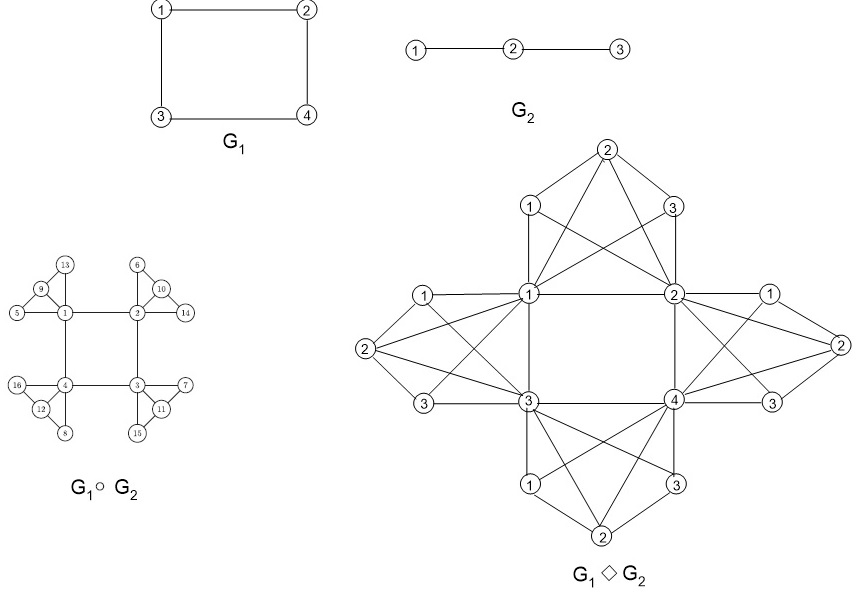
A lot of new graphs are obtained using new operations such as disjoint union, the Cartesian product, Kronecker product, the corona, the edge corona, the subdivision-vertex join, the subdivision-edge join, the vertex neighborhood corona and the subdivision-edge neighborhood corona. The adjacency spectra (Laplacian and signless Laplacian) of these operations have been calculated in Brouwer ; CDS ; CRS . So many infinite families of pairs of adjacency, Laplacian and signless Laplacian Isospectral graphs are generated using graph operation, see for example WZ ; RF ; LZ ; LZ1 ; MM ; BPS . Before going further let have some basic definitions which come from Fharray ; YW . Let $G_{1}$ and $G_{2}$ be two graphs on disjoint sets of $n_{1}$ and $n_{2}$ vertices with $m_{1}$ and $m_{2}$ edges respectively. The corona $G_{1}\circ G_{2}$ of $G_{1}$ and $G_{2}$ is defined as the graph obtained by taking one copy of $G_{1}$ and $n_{1}$ copies of $G_{2}$, then joining the $i^{th}$ vertex of $G_{1}$ to every vertex in the $i^{th}$ copy of $G_{2}$, see Figure(1). So in that way $G_{1}\circ G_{2}$ has $n_{1}(n_{2}+1)$ vertices with $m_{1}+n_{1}(m_{2}+n_{2})$ edges. Let $G_{1}$ and $G_{2}$ be two graphs on disjoint sets of $n_{1}$ and $n_{2}$ vertices, $m_{1}$ and $m_{2}$ edges, respectively. The edge coronal $G_{1}\lozenge G_{2}$ of two graphs is defined by taking one copy of $G_{1}$ and $m_{1}$ copies of $G_{2}$ and then joining two end vertices of the $i^{th}$ edge of $G_{1}$ to the every vertex in the $i^{th}$ copy of $G_{2}$, see Figure(1). So that the edge corona $G_{1}\lozenge G_{2}$ of $G_{1}$ and $G_{2}$ has $n_{1}+m_{1}n_{2}$ vertices and $m_{1}+2m_{1}n_{2}+m_{1}m_{2}$ edges.

Figure 1: vertex corona and edge corona of $G_{1}=C_{4}$ and $G_{2}=P_{3}$.

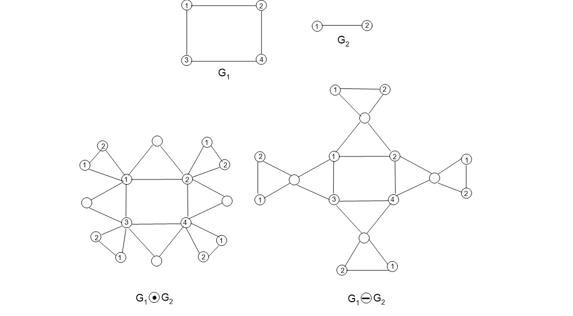
Similar to above we considered an another family of graph defined in LZhou . For a graph $G$, Let $R(G)$ be the graph obtained from the graph by adding a vertex $v_{e}$ and joining $v_{e}$ to the end vertices of $e$ for each $e\in E(G)$. The graph $R(G)$ appeared in CDS and named as the $R$-graph of $G$. In other words $R(G)$ is just the edge corona of $G$ and a singleton graph. Let $I(G)$ be the set of newly added vertices, i.e. $I(G)=V(R(G))\setminus V(G)$. Let $G_{1}$ and $G_{2}$ be two vertex disjoint graphs with $n_{1}$, $n_{2}$ vertices and $m_{1}$ and $m_{2}$ edges respectively. The $R$-vertexcorona of $G_{1}$ and $G_{2}$, denoted by $G_{1}\odot G_{2}$, is the graph obtained from vertex disjoint $R(G_{1})$ and $n_{1}$ copies of $G_{2}$ by joining the $i^{th}$ vertex of $V(G_{1})$ to every vertex in the $i^{th}$ copy of $G_{2}$, see Figure(2). So we have $n_{1}(1+n_{2})+m_{1}$ vertices in $G_{1}\odot G_{2}$ with $3m_{1}+n_{1}(m_{2}+n_{2})$ edges. The $R$-edgecorona of $G_{1}$ and $G_{2}$, denoted by $G_{1}\circleddash G_{2}$ is the graph obtained from vertex disjoint $R(G_{1})$ and $|I(G_{1})|$ copies of $G_{2}$ by joining the $i^{th}$ vertex of $I(G_{1})$ to every vertex in the $i^{th}$ copy of $G_{2}$, see Figure(2). Thus $G_{1}\circleddash G_{2}$ has $n_{1}+m_{1}(1+n_{2})$ vertices with $m_{1}(3+m_{2}+n_{2})$ edges.

Figure 2: $R$-vertexcorona and $R$-edgecorona of $G_{1}=C_{4}$ and $G_{2}=K_{2}$.

Motivated by researcher, we discuss the spectrum of above mention graphs using a new family of matrices introduced in Vildo which is in fact the convex combination of $A(G)$ and $D(G)$ defined by

$$A_{\alpha}(G)=\alpha D(G)+(1-\alpha)A(G),0\leq\alpha\leq 1.$$ (1.1)

So for $\alpha=0$ and $\alpha=\frac{1}{2}$ the equation(1.1) is similar to adjacency and signless Laplacian matrices of the graph. Let $M$ be an $n\times n$ matrix then $f_{M}(\theta)=(\theta I-M)$ is the characteristic polynomial of $M$, where $\sigma(M)$ will be considered as set of eigenvalues of matrix $M$. For any graph $G$, $f_{A_{\alpha}}(\nu)$ is the $A_{\alpha}$ characteristic polynomial of graph $G$. Denote $\nu_{1}\geq...\geq\nu_{n}$ be the $\alpha$-eigenvalues of the graph. The rest of the paper is organized as fallows. In Section $2$, we provided some Preliminaries. In Section $3$, we computed the $A_{\alpha}$ characteristic polynomial of $G_{1}\circ G_{2}$ when $G_{1}$ is any graph and $G_{2}$ is a regular(or complete bipartite) graph. In Section $4$, we computed the $A_{\alpha}$ characteristic polynomials of $G_{1}\lozenge G_{2}$ for a regular graph $G_{1}$ and any arbitrary graph $G_{2}$. In Section $5$, and Section $6$ we computed the $A_{\alpha}$ characteristic polynomials of of $G_{1}\odot G_{2}$ and $G_{1}\circleddash G_{2}$. In last we discussed, as an application of these results and mentioned a pairs of non isomorphic $\alpha$-Isospectral graphs through which we can generate infinitely many family of $\alpha$-Isospectral graphs.

2 Preliminaries

The symbol $\mathbf{0_{n}},\mathbf{j_{n}}$ (resp,$\mathbf{0_{mn}}$ and $\mathbf{J_{mn}}$) will stand for the column vector (resp, $m\times n$ matrices) consisting entirely of $0^{\prime}$s and $1^{\prime}$s. Also some standards notations $P_{n},C_{n}$ and $K_{a,b}$ for the path, cycle on $n$ vertices and complete bipartite graph on $n=a+b$ vertices. Let $G$ be a graph of order $n$ and $M$ be a graph of a matrix of $G$ the characteristic matrix $\theta I-M$ has determinant $det(\theta I-M)=f_{M}(\theta)\neq 0$, so is invertible. The $M-$coronal of an $n\times n$ square matrix $M$ denoted by $\Gamma_{M}(\theta)$, defined in SG , to be the sum of the entries of the matrix $(xI-M)^{-1}$, that is

$$\Gamma_{M}(\theta)=\mathbf{j^{T}_{n}}(\theta I-M)^{-1}\mathbf{j_{n}}.$$ (2.1)

It is known in SG that if each row sum of $M$ equals to a constant $t$, then equation. (2.1) has the form

$$\Gamma_{M}(\theta)=\frac{n}{\theta-t}.$$ (2.2)

The vertex-egde incidence matrix $B(G)$ of a graph is the $(0,1)$-matrix with rows and columns indexed by the vertices and edges of $G$, respectively, such that $ue$-entry is $1$ if and only if vertex $u$ in incident with edge $e$. It is a known fact that $BB^{T}=Q(G)$ also their is an alternative way of writing equation(1.1) as

$$Q(G)=\frac{1}{\beta}(A_{\alpha}(G)-(2\alpha-1)D(G)),$$ (2.3)

where $\beta=1-\alpha$ and $0\leq\alpha<1$. So we can write equation (2.3) as $BB^{T}=\beta^{-1}(A_{\alpha}(G)-(2\alpha-1)D(G))$. We also need to recall some elementary results from Linear Algebra on the multiplication of Kronecker products and determinants of block matrices.

• If $A$ is an $m\times n$ matrix and $B$ is a $p\times q$ matrix, then the Kronecker product $A\otimes B$ is the $mp\times nq$ block matrix.

• For any scalar $c$ we have $cA\otimes B=A\otimes cB=c(A\otimes B)$.

• $(A\otimes B)^{-1}=A^{-1}\otimes B^{-1}$ and $det(A\otimes B)=det(A)^{n}det(B)^{m}$, if $A$ and $B$ are $n\times n$ and $m\times m$ matrices respectively.

• If $A$ and $C$ are matrices of the same size, $B$ and $D$ are matrices of the same size, then $(A\otimes B)(C\otimes D)=(AC)\otimes(BD)$.

• If $D$ is invertible then

  $$det\begin{bmatrix}A&B\\ C&D\end{bmatrix}=det(D)det(A-BD^{-1}C).$$

3 $\alpha$-eigenvalue of $G_{1}\circ G_{2}$

Let $V(G_{1})=\{u_{1},...,u_{n_{1}}\}$ and $V(G_{2})=\{v_{1},...,v_{n_{2}}\}$ be two graphs on disjoint sets of $n_{1}$ and $n_{2}$ vertices with $m_{1}$ and $m_{2}$ edges respectively. Then $G=G_{1}\circ G_{2}$ has a partition $V(G)=V(G_{1})\cup V(G_{2})$. Obviously the degrees of the vertices in $G=G_{1}\circ G_{2}$ are:

$$d_{G_{1}\circ G_{2}}(u_{i}) =d_{G_{1}}(u_{i})+n_{2}fori=1,...,n_{1},$$

$$d_{G_{1}\circ G_{2}}(v_{j}) =d_{G_{2}}(v_{j})+1forj=1,...,n_{2}.$$

Then $A_{\alpha}(G)$ can be written as.

$$A_{\alpha}(G)=\begin{bmatrix}A_{\alpha}(G_{1})+\alpha n_{2}I_{n_{1}}&\mathbf{j_{n_{2}}^{T}}\otimes\beta I_{n_{1}}\\ \mathbf{j_{n_{2}}}\otimes\beta I_{n_{1}}&(A_{\alpha}(G_{2})+\alpha I_{n_{2}})\otimes I_{n_{1}}\end{bmatrix},$$

where $\beta=1-\alpha$.

Proposition 3.1.

Let $G_{1}$ and $G_{2}$ be two graphs on $n_{1}$ and $n_{2}$ vertices, respectively. Also let $\Gamma_{A_{\alpha}(G_{2})}(\nu)$ be the $A_{\alpha}(G_{2})$-coronal of $G_{2}$. Then the characteristic polynomial of $G=G_{1}\circ G_{2}$ is

$$f_{A_{\alpha}(G)}(\nu)=(f_{A_{\alpha}(G_{2})}(\nu-\alpha))^{n_{1}}\cdot f_{A_{\alpha}(G_{1})}(\nu-\alpha n_{2}-\beta^{2}\Gamma_{A_{\alpha}(G_{2})}(\nu-\alpha)),$$

In particularly, the $\alpha$-eigenvalue of $G$ is completely determined by the characteristics polynomial $f_{A_{\alpha}(G_{1})}$ and$f_{A_{\alpha}(G_{2})}$, and the $A_{\alpha(G_{2})}$ of $G_{2}$.

Proof.

The characteristic polynomial of $A_{\alpha}(G)$ can be calculated as fallows,

$$f_{A_{\alpha}(G)}(\nu)=det(\nu I_{n_{1}(n_{2}+1)}-A_{\alpha}(G)).$$

Which implies

$$=det\begin{bmatrix}\nu I_{n_{1}}-(A_{\alpha}(G_{1})+\alpha n_{2}I_{n_{1}})&-\mathbf{j_{n_{2}}^{T}}\otimes\beta I_{n_{1}}\\ -\mathbf{j_{n_{2}}}\otimes\beta I_{n_{1}}&\nu I_{n_{1}n_{2}}-(A_{\alpha}(G_{2})+\alpha I_{n_{2}})\otimes I_{n_{1}}\end{bmatrix},$$

$$=det\begin{bmatrix}(\nu-\alpha n_{2})I_{n_{1}}-A_{\alpha}(G_{1})&-\mathbf{j_{n_{2}}^{T}}\otimes\beta I_{n_{1}}\\ -\mathbf{j_{n_{2}}}\otimes\beta I_{n_{1}}&((\nu-\alpha)I_{n_{2}}-A_{\alpha}(G_{2}))\otimes I_{n_{1}}\end{bmatrix},$$

$$=det((\nu-\alpha)I_{n_{2}}-A_{\alpha}(G_{2}))\cdot det(B).$$

Where

$$B=(\nu-\alpha n_{2})I_{n_{1}}-A_{\alpha}(G_{1})-\beta^{2}(\mathbf{j_{n_{2}}^{T}}\otimes I_{n_{1}})((\nu-\alpha)I_{n_{2}}-A_{\alpha}(G_{2}))^{-1}(\mathbf{j_{n_{2}}}\otimes I_{n_{1}}),$$

and

$$det(B)=det\biggl{(}(\nu-\alpha n_{2})I_{n_{1}}-A_{\alpha}(G_{1})-\beta^{2}(\mathbf{j_{n_{2}}^{T}}((\nu-\alpha)I_{n_{2}}-A_{\alpha}(G_{2}))^{-1}\mathbf{j_{n_{2}}})\otimes I_{n_{1}})\biggr{)}.$$

Using equation (2.1) we get

$$det(B) =det((\nu-\alpha n_{2}-\beta^{2}\Gamma_{A_{\alpha}(G_{2})}(\nu-\alpha))I_{n_{1}}-A_{\alpha}(G_{1})),$$

$$=f_{A_{\alpha}(G_{1})}(\nu-\alpha n_{2}-\beta^{2}\Gamma_{A_{\alpha}(G_{2})}(\nu-\alpha)).$$

Hence the characteristic polynomial of $A_{\alpha}(G)$ is

$$f_{A_{\alpha}(G)}(\nu)=(f_{A_{\alpha}(G_{2})}(\nu-\alpha))^{n_{1}}\cdot f_{A_{\alpha}(G_{1})}(\nu-\alpha n_{2}-\beta^{2}\Gamma_{A_{\alpha}(G_{2})}(\nu-\alpha)),$$

This completes the proof. ∎

Following Theorem is an easy consequence of Proposition(3.1) and equation(2.2) when $G_{2}$ is $k$-regular.

Theorem 3.2.

Let $G_{1}$ be any graph on $n_{1}$ vertices and $G_{2}$ be a $k$-regular graph on $n_{2}$ vertices. Suppose $\sigma(G_{1})=\{\nu_{1},\nu_{2},...,\nu_{n}\}$ and $\sigma(G_{2})=\{k=\eta_{1},\eta_{2},...,\eta_{n}\}$ are the $\alpha$-eigenvalues of $G_{1}$ and $G_{2}$. Then the $\alpha$-eigenvalue of $G=G_{1}\circ G_{2}$ is given by:

• Two multiplicity- one eigenvalues

  $$\frac{\nu_{i}+k+\alpha(n_{2}+1)\pm\sqrt{\alpha^{2}n_{2}^{2}+(k+\alpha-\nu_{i})^{2}+2n_{2}(2+\alpha(\nu_{i}+\alpha-k-4))}}{2},$$

  for each eigenvalue $\nu_{i}(i=1,...,n)$ of $A_{\alpha}(G_{1})$.

• The $\alpha$-eigenvalue $\eta_{j}+1$ with multiplicity $n_{1}$ for every non maximal $\alpha$-eigenvalue $\eta_{j}$ $(j=1,...,n_{2}-1)$.

Proof.

Since $G_{2}$ is $k$-regular and so each row sum is $k$ using equation (2.2) that is,

$$\Gamma_{A_{\alpha}(G_{2})}(\eta-\alpha)=\frac{n_{2}}{(\eta-\alpha)-k},$$

$\eta=k+\alpha$ is the only pole in above equation. Which is equivalent to the maximal $\alpha$-eigenvalue $\eta-\alpha=k$ of $G_{2}$. Using Proposition(3.1), the $2n_{1}$ $\alpha$-eigenvalues are obtained by solving

$$\eta-\alpha n_{2}-\beta^{2}\frac{n_{2}}{\eta-\alpha-k}=\nu_{i}.$$

This equation is quadratic in $\eta$, that is,

$$\eta^{2}-(\alpha(n_{2}+1)+k+\nu_{i})\eta+\alpha n_{2}(\alpha+k+\nu_{i})-\beta^{2}n_{2}+k\nu_{i}=0,$$

for each $\alpha$-eigenvalue $\nu_{i}$ of $A_{\alpha}(G_{1})$.
Similarly the other $\eta_{1}(\eta_{2}-1)$ $\alpha$-eigenvalues are $\eta_{j}+1$ with multiplicity $n_{1}$ for every non maximum $\alpha$-eigenvalues $\eta_{j}$ , $j=1,...,n_{2}-1$. ∎

Now we will consider the $\alpha$-eigenvalue of $G=G_{1}\circ G_{2}$ when $G_{1}$ is any graph and $G_{2}=K_{a,b}$. If $a=b$, then $G_{2}$ is $a$-regular graph, which has been exhibited in Theorem(3.2). It is always assumed that $a\neq b$ in the following Theorem.

Theorem 3.3.

Let $G_{1}$ be any graph on $n_{1}$ vertices and $G_{2}=K_{a,b}$ on $n_{2}=a+b$ vertices. Suppose that $\sigma(G_{1})=\{\nu_{1},\nu_{2},...,\nu_{n}\}$. Then the $\alpha$-eigenvalue of $G=G_{1}\circ G_{2}$ consists preciely of:

• The $\alpha$-eigenvalue $\alpha(a+1)$ with multiplicity $n_{1}(b-1)$.

• The $\alpha$-eigenvalue $\alpha(b+1)$ with multiplicity $n_{1}(a-1)$.

• For each $\alpha$-eigenvalue $\nu_{i}$ ($i=1,2,...,n_{1}$) of $A_{\alpha}(G)$, $\eta_{i1}+\alpha,\eta_{i2}+\alpha,\eta_{i2}+\alpha$ are three $\alpha$-eigenvalue of $G$ where $\eta_{i1},\eta_{i2},\eta_{i3}$ are the three roots of polynomial

  $$\eta^{3}+\eta^{2}(-\nu_{i}-2\alpha n_{2})+\eta(a(2\alpha-1)b+n_{2}(\alpha(\nu_{i}+\alpha n_{2})-1))-2ab\\ +\alpha n_{2}(a(1-2\alpha)b+n_{2})+a(1-2\alpha)b\nu_{i}=0.$$

Proof.

We first compute the $A_{\alpha}(G_{2})$-coronal of $G_{2}=K_{a,b}$, Let

$$A_{\alpha}(G_{2})=\begin{bmatrix}\alpha bI_{a}&\beta\mathbf{J}\\ \beta\mathbf{J}&\alpha aI_{b}\end{bmatrix}.$$

Consider the diagonal matrix

$$X=\begin{bmatrix}(\eta-\alpha a+\beta b)I_{a}&\mathbf{0}\\ \mathbf{0}&(\eta-\alpha b+\beta a)I_{b}\end{bmatrix}$$

By a simple calculation we get $(\eta I-A_{\alpha}(G_{2}))X\mathbf{j_{n_{2}}}=\eta^{2}-\alpha(a+b)\eta+(2\alpha-1)ab\mathbf{j_{n_{2}}}$. Hence

$$\Gamma_{A_{\alpha}(G_{2})}(\eta)=\mathbf{j_{n_{2}}^{T}}(\eta I-A_{\alpha}(G_{2}))\mathbf{j_{n_{2}}}=\frac{\eta(a+b)-\alpha(a^{2}+b^{2})+2(1-\alpha)ab}{\eta^{2}-\alpha(a+b)\eta+(2\alpha-1)ab},$$

$$=\frac{\eta n_{2}-\alpha n_{2}^{2}+2ab}{\eta^{2}-\alpha n_{2}\eta+(2\alpha-1)ab}.$$

As the $\alpha$-eigenvalue of $K_{a,b}$ is $\sigma(K_{a,b})=\{\frac{\alpha n+\sqrt{\alpha^{2}n^{2}+4ab(1-2\alpha)}}{2},[\alpha a]^{b-1}$,
$[\alpha b]^{a-1},\frac{\alpha n-\sqrt{\alpha^{2}n^{2}+4ab(1-2\alpha)}}{2}\}$. Where the two poles of $\Gamma_{A_{\alpha}(G_{2})}(\eta-\alpha)$ are $\eta=\alpha+\frac{\alpha n+\sqrt{\alpha^{2}n^{2}+4ab(1-2\alpha)}}{2}$ and $\eta=\alpha+\frac{\alpha n-\sqrt{\alpha^{2}n^{2}+4ab(1-2\alpha)}}{2}$. Using Proposition(3.1), the $\alpha$-eigenvalue of $G$ is given as $\alpha(a+1),\alpha(b+1)$ with multiplicity $n_{1}(b-1)$ and $n_{1}(a-1)$ respectively. While the other $3n_{1}$ eigenvalues are obtained by solving:

$$\eta-\alpha n_{2}-\Gamma_{A_{\alpha}(G_{2})}(\eta-\alpha)=\nu_{i},$$

that is

$$\eta-\alpha n_{2}-\frac{(\eta-\alpha)n_{2}-\alpha n_{2}^{2}+2ab}{(\eta-\alpha)^{2}-\alpha n_{2}(\eta-\alpha)+(2\alpha-1)ab}=\nu_{i}.$$

This equation is of degree three in $\eta$, that is,

$$2ab(1-2\alpha)+(a^{2}+b^{2})\alpha+n_{2}\alpha-n_{2}\alpha^{3}-n^{2}\alpha^{3}-abn_{2}\alpha(-1+2\alpha)+\eta^{3}+\eta^{2}(-2\alpha\\ -2n_{2}\alpha-\nu_{i})-\alpha^{2}\nu_{i}+n\alpha^{2}\nu_{i}+ab(-1+2\alpha)\nu_{i}+\eta(-n_{2}+\alpha^{2}+3n_{2}\alpha^{2}+n^{2}\alpha^{2}\\ +ab(-1+2\alpha)+2\alpha\nu_{i}-n_{2}\alpha\nu_{i})=0.$$

Simplifying above will lead us to,

$$a^{2}\alpha+\eta^{3}-ab(-1+2\alpha)(2+n_{2}\alpha-\nu_{i})+\eta^{2}(-2(1+n)\alpha-\nu_{i})+\alpha(b^{2}+n-n\alpha^{2}-n_{2}^{2}\alpha^{2}\\ -\alpha\nu_{i}+n_{2}\alpha\nu_{i})+\eta(n^{2}\alpha^{2}+ab(-1+2\alpha)+\alpha(\alpha+2\nu_{i})+n_{2}(-1+3\alpha^{2}-\alpha\nu_{i}))=0.$$

∎

As an application of the Theorem(3.3), we constructed pairs of $\alpha$-eigenvalue of graphs. By Proposition (3.1), the $\alpha$-eigenvalues of $G_{1}\circ G_{2}$ is completely determined by the characteristic polynomials $f_{A_{\alpha}(G_{1})}$ and $f_{A_{\alpha}(G_{2})}$ and the $A_{\alpha}(G_{2})$-coronal of $G_{2}$. Which leads us to following result.

Corollary 3.4.

Let $G_{1}$ and $G_{2}$ are two non-isomorphic $\alpha$-Isospectral graph, and $H$ be any graph. Then,

• $G_{1}\circ H$ and $G_{2}\circ H$ are non-isomorphic $\alpha$-Isospectral graphs.

• $H\circ G_{1}$ and $H\circ G_{2}$ are non-isomorphic $\alpha$-Isospectral graphs whenever $\Gamma_{A_{\alpha}(G_{1})}=\Gamma_{A_{\alpha}(G_{2})}$.

4 $\alpha$-eigenvalue of $G_{1}\lozenge G_{2}$

Let the vertex set of a graph $G_{1}$ and $G_{2}$ be $V(G_{1})=\{u_{1},u_{2},...,u_{n_{1}}\}$ and $V(G_{2})=\{v_{1},v_{2},...,v_{n_{2}}\}$, respectively. Where the edge set of graph $G_{1}$ is $E(G_{1})=\{e_{1},e_{2},...,e_{m_{1}}\}$. The vertex-edge incidence matrix $B_{1}(G)=(b_{ue})$ is an $n_{1}\times m_{1}$ matrix with entry $b_{ue_{j}}=1$ if the vertex $u$ is incident the edge $e_{j}$ and $0$ otherwise. Let $G_{1}$ be $k_{1}$ regular graph and $G_{2}$ be any graph. Then the graph $G=G_{1}\lozenge G_{2}$ has the partition $V(G)=V(G_{1})\cup V(G_{2})$. The degree of the vertices in $G_{1}\lozenge G_{2}$ are:

$$d_{G_{1}\lozenge G_{2}}(u_{i}) =d_{G_{1}}(u_{i})+k_{1}n_{2}fori=1,...,n_{1},$$

$$d_{G_{1}\lozenge G_{2}}(v_{j}) =d_{G_{2}}(v_{j})+2forj=1,...,n_{2}.$$

Then using equation (1.1), the $A_{\alpha}$ matrix of $G=G_{1}\lozenge G_{2}$ is written as:

$$A_{\alpha}(G)=\begin{bmatrix}A_{\alpha}(G_{1})+\alpha k_{1}n_{2}I_{n_{1}}&B_{1}\otimes\beta\mathbf{j_{n_{2}}^{T}}\\ B_{1}^{T}\otimes\beta\mathbf{j_{n_{2}}}&I_{m_{1}}\otimes(2\alpha I_{n_{2}}+A_{\alpha}(G_{2}))\end{bmatrix}$$

where $\beta=1-\alpha$.

Remark 4.1.

Using fact $BB^{T}=Q(G)$ and equation (2.3). If a graph $G$ is $k$ regular then $BB^{T}=\beta^{-1}(A_{\alpha}(G)-(2\alpha-1)kI)$.

Theorem 4.1.

Let $G_{1}$ be an $k_{1}$ regular graph $n_{1}$ vertices, $m_{1}$ edges and $G_{2}$ be any graph with $n_{2}$ vertices, $m_{1}$ edges. Also let $\Gamma_{A_{\alpha}(G_{2})}(\nu)$ be the $A_{\alpha}(G_{2})$-coronal of $G_{2}$. if $\nu$ is not a pole of $\Gamma_{A_{\alpha}(G_{2})}(\nu-2\alpha)$.

$$f_{A_{\alpha}(G)}(\nu)=(f_{A_{\alpha}(G_{2})}(\nu-2\alpha))^{m_{1}}\cdot f_{A_{\alpha}(G_{1})}\left(\frac{\nu-\alpha k_{1}n_{2}+\beta k_{1}(2\alpha-1)}{1+\beta\Gamma_{A_{\alpha}(G_{2})}(\nu-2\alpha)}\right)\cdot\\ \left[1+\beta\Gamma_{A_{\alpha}(G_{2})}(\nu-2\alpha)\right]^{n_{1}}.$$

Proof.

The characteristic polynomial of $A_{\alpha}(G)$ can be calculated as fallows,

$$f_{A_{\alpha}(G)}(\nu)=det(\nu I_{n_{1}+m_{1}n_{2}}-A_{\alpha}(G)).$$

So we have,

$$=det\begin{bmatrix}\nu I_{n_{1}}-(A_{\alpha}(G_{1})+\alpha k_{1}n_{2}I_{n_{1}})&-B_{1}\otimes\beta\mathbf{j_{n_{2}}^{T}}\\ -B_{1}^{T}\otimes\beta\mathbf{j_{n_{2}}}&\nu I_{m_{1}n_{2}}-I_{m_{1}}\otimes(2\alpha I_{n_{2}}+A_{\alpha}(G_{2}))\end{bmatrix},$$

$$=det\begin{bmatrix}(\nu-\alpha k_{1}n_{2})I_{n_{1}}-A_{\alpha}(G_{1})&-B_{1}\otimes\beta\mathbf{j_{n_{2}}^{T}}\\ -B_{1}^{T}\otimes\beta\mathbf{j_{n_{2}}}&I_{m_{1}}\otimes((\nu-2\alpha)I_{n_{2}}-A_{\alpha}(G_{2}))\end{bmatrix},$$

$$=det(I_{m_{1}}\otimes(\nu-2\alpha)I_{n_{2}}-A_{\alpha}(G_{2}))\cdot det(S).$$

where $S=((\nu-\alpha k_{1}n_{2})I_{n_{1}}-A_{\alpha}(G_{1})-B_{1}B_{1}^{T}\otimes\beta^{2}(\mathbf{j^{T}_{n_{2}}}((\nu-2\alpha)I_{n_{2}}-A_{\alpha}(G_{2}))^{-1}\mathbf{j_{n_{2}}}))$.
Using Remark(4.1) and equation (2.2) we get,

$$S =((\nu-\alpha k_{1}n_{2})I_{n_{1}}-A_{\alpha}(G_{1})-(A_{\alpha}(G_{1})-(2\alpha-1)I_{n_{2}})\otimes\beta\Gamma_{A_{\alpha}(G_{2})}(\nu-2\alpha)),$$

$$=((\nu-\alpha k_{1}n_{2}+\beta(2\alpha-1)\Gamma_{A_{\alpha}(G_{2})}(\nu-2\alpha))I_{n_{1}}-(1+\beta\Gamma_{A_{\alpha}(G_{2})}(\nu-2\alpha)A_{\alpha}(G_{1})).$$

$$det(S) =det(((\nu-\alpha k_{1}n_{2}+\beta(2\alpha-1)\Gamma_{A_{\alpha}(G_{2})}(\nu-2\alpha))I_{n_{1}}-(1+\beta\Gamma_{A_{\alpha}(G_{2})}(\nu-2\alpha)A_{\alpha}(G_{1}))).$$

$$=f_{A_{\alpha}(G_{1})}\left(\frac{\nu-\alpha k_{1}n_{2}+\beta k_{1}(2\alpha-1)}{1+\beta\Gamma_{A_{\alpha}(G_{2})}(\nu-2\alpha)}\right)\left[1+\beta\Gamma_{A_{\alpha}(G_{2})}(\nu-2\alpha)\right]^{n_{1}}.$$

Here completes the proof.

∎

Theorem 4.2.

Let $G_{1}$ be $k_{1}$-regular graph on $n_{1}$ vertices and $G_{2}$ be a $k_{2}$-regular graph on $n_{2}$ vertices. Suppose $\sigma(G_{1})=\{k_{1}=\nu_{1},\nu_{2},...,\nu_{n}\}$ and $\sigma(G_{2})=\{k_{2}=\eta_{1},\eta_{2},...,\eta_{n}\}$ are the $\alpha$-eigenvalues of $G_{1}$ and $G_{2}$ respectively. Then the $\alpha$-eigenvalue of $G=G_{1}\lozenge G_{2}$ is given by:

• The $\alpha$-eigenvalue $\eta_{j}+2\alpha$ with multiplicity $m_{1}$ for every non maximal $\alpha$-eigenvalue $\eta_{j}$ ($j=1,...,m_{1}$) of $A_{\alpha}(G_{2})$.

• Two multiplicity one $\alpha$-eigenvalues by solving,
  $\eta^{2}+\eta(-2\alpha-k_{2}-k_{1}(1-3\alpha+2\alpha^{2}+\alpha n_{2})-\nu_{i})+k_{1}(2\alpha+k_{2})(1-3\alpha+2\alpha^{2}+\alpha n_{2})+(2\alpha+k_{2}+(-1+\alpha)n_{2})\nu_{i}=0$,
  for each $\alpha$-eigenvalue $\nu_{i}$, for ($i=1,...,n_{1}$), $A_{\alpha}(G_{1})$, and

• The $\alpha$-eigenvalue $k_{2}+2\alpha$ with multiplicity $m_{1}-n_{1}$(if possible).

Proof.

As $G_{2}$ is $k_{2}$ regular, each row sum of $A_{\alpha}(G_{2})$ is $k_{2}$, using equation (2.2)

$$\Gamma_{A_{\alpha}(G_{2})}(\eta-2\alpha)=\frac{n_{2}}{\eta-2\alpha-k_{2}}.$$

The only pole in above equation is $\eta=2\alpha+k_{2}$, which is equivalent to the maximal $\alpha$-eigenvalue $\eta-2\alpha=k_{2}$ of $G_{2}$. Now suppose that $\eta$ is not the pole in above equation. Then by Theorem(4.1), one has

• The $m_{1}(n_{2}-1)$ $\alpha$-eigenvalues are $\eta_{j}+2\alpha$ with multiplicity $m_{1}$ for every non maximal $\alpha$-eigenvalue $\eta_{j}$, (for $j=1,...,n_{2}-1$), of $A_{\alpha}(G_{2})$ and

• For each $\alpha$-eigenvalue $\nu_{i}$, for ($i=1,...,n_{1}$), of $A_{\alpha}(G_{1})$. The $2n_{1}$ eigenvalues are obtained by solving, which is quadratic in $\eta$,

  $$\eta-\alpha k_{1}n_{2}+\beta k_{1}(2\alpha-1)=\nu_{i}(1+\beta\frac{n_{2}}{\eta-2\alpha-k_{2}}),$$

  $$\eta^{2}-2(1-\alpha)\alpha(-1+2\alpha)k_{1}-(1-\alpha)(-1+2\alpha)k_{1}k_{2}+2\alpha^{2}k_{1}n_{2}+\alpha k_{1}k_{2}n_{2}\\ +\eta(-2\alpha+(1-\alpha)(-1+2\alpha)k_{1}-k_{2}-\alpha k_{1}n_{2}-\nu_{i}+2\alpha\nu_{i}+k_{2}\nu_{i}-(1-\alpha)n_{2}\nu_{i}=0,$$

  $$\eta^{2}+k_{1}(2\alpha+k_{2})(1-3\alpha+2\alpha^{2}+\alpha n_{2})+\eta(-2\alpha-k_{2}-k_{1}(1-3\alpha+2\alpha^{2}\\ +\alpha n_{2})-\nu_{i})+(2\alpha+k_{2}+(-1+\alpha)n_{2})\nu_{i}=0.$$

We get $m_{1}(n_{2}-1)+2n_{1}$, $\alpha$-eigenvalues of $G$. The other $n_{1}+m_{1}n_{2}-(m_{1}(n_{2}-1)+2n_{1})=m_{1}-n_{1}$ $\alpha$-eigenvalues of $G$ must come from the only pole $\eta=k_{2}+2\alpha$ of $\Gamma_{A_{\alpha}(G_{2})}(\eta-2\alpha)$. ∎

Next we will give a little more description of $\alpha$-eigenvalue of $G_{1}\lozenge G_{2}$ when $G_{1}$ is $k_{1}$-regular and $G_{2}=K_{a,b}$.

Theorem 4.3.

Let $G_{1}$ be $k_{1}$-regular graph on $n_{1}$ vertices and $G_{2}=K_{a,b}$ on $n_{2}=a+b$ vertices and $m_{2}$ edges. Suppose $\sigma(G_{1})=\{k_{1}=\nu_{1},\nu_{2},...,\nu_{n}\}$. Then the $\alpha$-eigenvalue of $G=G_{1}\lozenge G_{2}$ is given by:

• The $\alpha$-eigenvalue $\alpha(a+2)$ with multiplicity $m_{1}(b-1)$.

• The $\alpha$-eigenvalue $\alpha(b+2)$ with multiplicity $m_{1}(a-1)$.

• For each $\alpha$-eigenvalue $\nu_{i}$ ($i=1,2,...,n_{1}$) of $A_{\alpha}(G_{1})$, $\eta_{i1}+2\alpha,\eta_{i2}+2\alpha$ and $\eta_{i3}+2\alpha$ are three $\alpha$-eigenvalues of $G$ where $\eta_{i1},\eta_{i2}$ and $\eta_{i3}$ are three roots of cubic polynomial polynomial in $\eta$

  $$\eta^{3}+(((3-2\alpha)\alpha-\nu_{i}-1)k_{1}-\alpha(k+1)n_{2})\eta^{2}+\eta(a(2\alpha-1)b+n_{2}((2\alpha-1)\nu_{i}\\ +(\alpha-1)(2\alpha-1)\alpha k_{1}+\alpha^{2}kn_{2}))-\nu_{i}(-(ab+(\alpha-1)\alpha n_{2}^{2}))a(1-2\alpha)\alpha bkn_{2}\\ -a(1-2\alpha)^{2}(\alpha-1)bk_{1}=0.$$

• The $\alpha$-eigenvalue $\{\frac{\alpha(n+4)\pm\sqrt{\alpha^{2}n^{2}+4ab(1-2\alpha)}}{2}\}$ with multiplicity $m_{1}-n_{1}$(if possible).

Proof.

Using Theorem (3.3)and Theorem (4.1)) we can easily deduce $i,ii$ and $iv$.

• Solving $\eta-k_{1}(1-3\alpha+2\alpha^{2}+\alpha n_{2})=\nu_{i}(1+\beta\Gamma_{A_{\alpha}(G_{2})}(\eta-2\alpha))$, we get a little ugly equation

  $$\eta^{3}+\eta^{2}(-4\alpha-k_{1}(2\alpha^{2}-3\alpha+\alpha n_{2}+1)-\nu+\alpha n_{2})+\eta(2a(2\alpha-1)b+4\alpha(\alpha+\nu)\\ -\alpha k_{1}(n_{2}-4)(2\alpha^{2}-3\alpha+\alpha n_{2}+1)+(\alpha-1)\nu n_{2}^{2}-\alpha n_{2}(2\alpha+\nu))+2(k_{1}(2\alpha^{2}-3\alpha\\ +\alpha n_{2}+1)(-2\alpha^{2}-2a\alpha b+ab+\alpha^{2}n_{2})+\alpha\nu(-ab-2\alpha+n_{2}(\alpha-(\alpha-1)n_{2})))=0.$$

∎

Corollary 4.4.

Suppose that $G_{1}$, $G_{2}$ are two non-isomorphic $A_{\alpha}$-Isospectral $k$-regulars graphs. If $H=K_{a,b}$ then $G_{1}\lozenge H$ and $G_{2}\lozenge H$ also are non isomorphic $A_{\alpha}$-Isospectral graphs.

5 $\alpha$-eigenvalue of $R$-vertex coranae

Let $V(G_{1})=\{u_{1},...,u_{n_{1}}\}$, $I(G)=\{w_{1},...,w_{m_{1}}\}$ and $V(G_{2})=\{v_{1},...,v_{n_{1}}\}$. For $i=1,...,n_{1}$, let $V^{i}(G_{2})=\{v^{i}_{1},...,v^{i}_{n_{2}}\}$ be the vertex set of the $i^{th}$ copy of $G_{2}$. Then $V(G_{1}\odot G_{2})$ has a partition

$$V(G_{1})\cup I(G_{1})\cup\biggl{(}\bigcup_{i=1}^{n_{1}}V^{i}(G_{2})\biggr{)}.$$ (5.1)

So the degrees of the vertices of $G_{1}\odot G_{2}$ are:

$$d_{G_{1}\odot G_{2}}(u_{i}) =2d_{G_{1}}(v_{i})+n_{2}fori=1,...,n_{1},$$

$$d_{G_{1}\odot G_{2}}(w_{i}) =2fori=1,...,m_{1},$$

$$d_{G_{1}\odot G_{2}}(u^{i}_{j}) =d_{G_{2}}(v_{j})+1fori=1,...,n_{1}andforj=1,...,n_{2}.$$

Considering the $\alpha$-eigenvalue of this graph. The equation(1.1), of $G=G_{1}\odot G_{2}$ with respect to the partition (5.1) can be written as fallows,

$$A_{\alpha}(G)=\begin{bmatrix}A_{\alpha}(G_{1})&\beta B_{1}&\beta I_{n_{1}}\otimes\mathbf{j^{T}_{n_{2}}}\\ \beta B_{1}^{T}&2\alpha I_{m_{1}}&\mathbf{O_{m_{1}\times n_{1}n_{2}}}\\ \beta I_{n_{1}}\otimes\mathbf{j_{n_{2}}}&\mathbf{O_{m_{1}\times n_{1}n_{2}}}&I_{n_{1}}\otimes A_{\alpha}(G_{2})\end{bmatrix},$$

where $\beta=1-\alpha$

Theorem 5.1.

Let $G_{1}$ be an $k_{1}$-regular graph with $n_{1}$ vertices, and $G_{2}$ be an arbitrary graph with $n_{2}$ vertices. Then the characteristics polynomial of $G=G_{1}\odot G_{2}$ is

$$$$f_{A_{\alpha}(G)}(\nu)=(\nu-2\alpha)^{m_{1}-n_{1}}\cdot\prod_{i=1}^{n_{2}}(\nu-\alpha-\nu_{i}(G_{2}))^{n_{1}}\cdot\\ \prod_{i=1}^{n_{1}}\Biggl{(}\nu^{2}-(k^{\prime}+\beta^{2}\Gamma_{A_{\alpha}(G_{2})}(\nu-k^{\prime})+2\alpha+\nu_{i}(G_{1}))\nu\\ +2\alpha k^{\prime}+2\alpha\beta^{2}\Gamma_{A_{\alpha}(G_{2})}(\nu-k^{\prime})+k^{\prime}\beta(2\alpha-1)-\beta\nu_{i}(G_{1})\Biggr{)},$$$$

where $k^{\prime}=\alpha(k_{1}+n_{2})$.

Proof.

Considering the partition (5.1), we have

$$A_{\alpha}(G) =\begin{bmatrix}A_{\alpha}(G_{1})+\alpha(k_{1}+n_{2})I_{n_{1}}&\beta B_{1}&\beta I_{n_{1}}\otimes\mathbf{j^{T}_{n_{2}}}\\ \beta B_{1}^{T}&2\alpha I_{m_{1}}&\mathbf{O_{m_{1}\times n_{1}n_{2}}}\\ \beta I_{n_{1}}\otimes\mathbf{j_{n_{2}}}&\mathbf{O_{m_{1}\times n_{1}n_{2}}}&I_{n_{1}}\otimes(A_{\alpha}(G_{2})+\alpha I_{n_{2}})\end{bmatrix}.$$

$$f_{A_{\alpha}(G)}(\nu) =det\begin{bmatrix}(\nu-\alpha(k_{1}+n_{2}))I_{n_{1}}-A_{\alpha}(G_{1})&-\beta B_{1}&-\beta I_{n_{1}}\otimes\mathbf{j^{T}_{n_{2}}}\\ -\beta B_{1}^{T}&(\nu-2\alpha)I_{m_{1}}&\mathbf{O_{m_{1}\times n_{1}n_{2}}}\\ -\beta I_{n_{1}}\otimes\mathbf{j_{n_{2}}}&\mathbf{O_{m_{1}\times n_{1}n_{2}}}&I_{n_{1}}\otimes((\nu-\alpha I_{n_{2}})-A_{\alpha}(G_{2}))\end{bmatrix},$$

$$=det(I_{n_{1}}\otimes((\nu-\alpha I_{n_{2}})-A_{\alpha}(G_{2})))\cdot detS$$

$$=\prod_{i=1}^{n_{2}}(\nu-\alpha-\nu_{i}(G_{2}))^{n_{1}}\cdot detS.$$

Where

$$S=\begin{bmatrix}(\nu-\alpha(k_{1}+n_{2}))I_{n_{1}}-A_{\alpha}(G_{1})&-\beta B_{1}&\\ -\beta B_{1}^{T}&(\nu-2\alpha)I_{m_{1}}\end{bmatrix}\\ -\begin{bmatrix}\beta I_{m_{1}}\otimes\mathbf{j^{T}_{n_{2}}}\\ \boldsymbol{O_{m_{1}\times n_{1}n_{2}}}\end{bmatrix}(I_{n_{1}}\otimes((x-\alpha)I_{n_{2}}-A_{\alpha}(G_{2})))^{-1}\begin{bmatrix}\beta I_{m_{1}}\otimes\mathbf{j_{n_{2}}}&\boldsymbol{O_{m_{1}\times n_{1}n_{2}}}\end{bmatrix},$$

Assume $\alpha(k_{1}+n_{2})=k^{\prime}$

$$S=\begin{bmatrix}(\nu-k^{\prime})I_{n_{1}}-A_{\alpha}(G_{1})&-\beta B_{1}&\\ -\beta B_{1}^{T}&(\nu-2\alpha)I_{m_{1}}\end{bmatrix}-\begin{bmatrix}\beta^{2}I_{n_{1}}\otimes\mathbf{j^{T}}(\nu-k^{\prime}I_{n_{2}}-A_{\alpha}(G_{2}))^{-1}\mathbf{j}&\mathbf{O}\\ \mathbf{O}&\mathbf{O}\end{bmatrix},$$

Using Remark(4.1) and equation (2.1) we have,

$$S =\begin{bmatrix}(\nu-k^{\prime}-\beta^{2}\Gamma_{A_{\alpha}(G_{2})}(\nu-k^{\prime}))I_{n_{1}}-A_{\alpha}(G_{1})&-\beta B_{1}\\ -\beta B_{1}^{T}&(\nu-2\alpha)I_{m_{1}}\end{bmatrix},$$

$$detS =(x-2\alpha)^{m_{1}}det((\nu-k^{\prime}-\beta^{2}\Gamma_{A_{\alpha}(G_{2})}(\nu-k^{\prime}))I_{n_{1}}-A_{\alpha}(G_{2})-\frac{\beta^{2}B_{1}B_{1}^{T}}{\nu-2\alpha}),$$

$$=(x-2\alpha)^{m_{1}}det((\nu-k^{\prime}-\beta^{2}\Gamma_{A_{\alpha}(G_{2})}(\nu-k^{\prime})+\frac{k_{1}\beta(2\alpha-1)}{\nu-2\alpha})I_{n_{1}}-(1+\frac{\beta}{\nu-2\alpha})A_{\alpha}(G_{1})),$$

$$=(x-2\alpha)^{m_{1}-n_{1}}\cdot\prod_{i=1}^{n_{1}}(\nu^{2}-(k^{\prime}+\beta^{2}\Gamma_{A_{\alpha}(G_{2})}(\nu-k^{\prime})\\ +2\alpha+\nu_{i}(G_{1}))\nu+2\alpha k^{\prime}+2\alpha\beta^{2}\Gamma_{A_{\alpha}(G_{2})}(\nu-k^{\prime})+k^{\prime}\beta(2\alpha-1)-\beta\nu_{i}(G_{1})).$$

Now the result fallows easily. ∎

Corollary 5.2.

Let $G_{1}$ be an $k_{1}$-regular graph with $n_{1}$ vertices,and $G_{2}$ be an $k_{2}$-regular graph with $n_{2}$ vertices. Then

$$f_{A_{\alpha}(G)}(\nu)=(\nu-2\alpha)^{m_{1}-n_{1}}\cdot\prod_{i=1}^{n_{2}}((\nu-\alpha-\nu_{i}(G_{2}))^{n_{1}})\cdot\\ \prod_{i=1}^{n_{1}}\Biggl{(}\nu^{3}-(2k^{\prime}+k_{2}+2\alpha+\nu_{i}(G_{1}))\nu^{2}+((k^{\prime}+k_{2})(k^{\prime}+2\alpha+\nu_{i}(G_{1}))-n_{2}\beta^{2}+2\alpha k^{\prime}\\ +\beta(k_{1}(2\alpha-1)-\nu_{i}(G_{2})))\nu-(k^{\prime}+k_{2})(2\alpha k^{\prime}+k_{1}\beta+\beta\nu_{i}(G_{2}))+2\alpha\beta^{2}k^{\prime}\Biggr{)},$$

where $k^{\prime}=\alpha(k_{1}+n_{2})$.

Proof.

Using Theorem(5.1) and equation(2.2) it is obvious. ∎

Corollary 5.3.

• If $G_{1}$ and $G_{2}$ are $\alpha$-Isospectral regular graphs, and $H$ is an arbitrary graph, then $G_{1}\odot H$ and $G_{2}\odot H$ are $\alpha$-Isospectral.

• If $G$ is a regular graph, and $H_{1}$ and $H_{2}$ are $\alpha$-Isospectral graphs with $\Gamma_{A_{\alpha}(H_{1})}(\nu)=\Gamma_{A_{\alpha}(H_{2})}(\nu)$, then $G_{1}\odot H$ and $G_{2}\odot H$ are $\alpha$-Isospectral.

• If $G_{1}$ and $G_{2}$ are $\alpha$-Isospectral regular graphs, and $H_{1}$ and $H_{2}$ are $\alpha$-Isospectral graphs with $\Gamma_{A_{\alpha}(H_{1})}(\nu)=\Gamma_{A_{\alpha}(H_{2})}(\nu)$, then $G_{1}\odot H$ and $G_{2}\odot H$ are $\alpha$-Isospectral.

6 $\alpha$-eigenvalue of $R$-edge coronae

Let $V(G_{1})=\{u_{1},...,u_{n_{1}}\}$, $I(G)=\{w_{1},...,w_{m_{1}}\}$ and $V(G_{2})=\{v_{1},...,v_{n_{1}}\}$. For $i=1,...,m_{1}$, let $V^{i}(G_{2})=\{v^{i}_{1},...,v^{i}_{n_{2}}\}$ be the vertex set of the $i^{th}$ copy of $G_{2}$. Then $V(G_{1}\odot G_{2})$ has a partition

$$V(G_{1})\cup I(G_{1})\cup\biggl{(}\bigcup_{i=1}^{m_{1}}V^{i}(G_{2})\biggr{)}.$$ (6.1)

So the degrees of the vertices of $G_{1}\odot G_{2}$ are:

$$d_{G_{1}\circleddash G_{2}}(u_{i}) =2d_{G_{1}}(v_{i})fori=1,...,n_{1},$$

$$d_{G_{1}\circleddash G_{2}}(w_{i}) =2+n_{2}fori=1,...,m_{1},$$

$$d_{G_{1}\circleddash G_{2}}(u^{i}_{j}) =d_{G_{2}}(u_{j})+1fori=1,...,m_{1}andforj=1,...,n_{2}.$$

Considering the $\alpha$-eigenvalue of this graph. The equation(1.1), of $G=G_{1}\circleddash G_{2}$ with respect to the partition (6.1) can be written as fallows,

$$A_{\alpha}(G)=\begin{bmatrix}A_{\alpha}(G_{1})+\alpha k_{1}I_{n_{1}}&\beta B_{1}&\mathbf{O_{n_{1}\times m_{1}n_{2}}}\\ \beta B_{1}^{T}&(n_{2}+2)\alpha I_{m_{1}}&\beta I_{m_{1}}\otimes\mathbf{j^{T}_{n_{2}}}\\ \mathbf{O_{m_{1}n_{2}\times n_{1}}}&\beta I_{m_{1}}\otimes\mathbf{j_{n_{2}}}&I_{m_{1}}\otimes(A_{\alpha}(G_{2})+\alpha I_{n_{1}})\end{bmatrix},$$

where $\beta=1-\alpha$.

Theorem 6.1.

Let $G_{1}$ be an $k_{1}$-regular graph with $n_{1}$ vertices and $m_{1}$ edges, and $G_{2}$ be an arbitrary graph with $n_{2}$ vertices. Then

$$f_{A_{\alpha}(G)}(\nu)=(\nu-r)^{m_{1}-n_{1}}\cdot\prod_{i=1}^{n_{2}}(\nu-\alpha-\nu_{i}(G_{2}))^{m_{1}}\cdot\\ \prod_{i=1}^{n_{1}}(\nu^{2}-(r+\alpha k_{1}+\nu_{i}(G_{1}))\nu+(\alpha r+\beta(2\alpha-1))k_{1}+(r-\beta)\nu_{i}(G_{1})),$$

where $(n_{2}+2)\alpha+\Gamma_{A_{\alpha}(G_{2})}(\nu-\alpha)=r$.

Proof.

Considering the partition (6.1)

$$f_{A_{\alpha}(G)}(\nu) =\begin{bmatrix}(\nu-\alpha k_{1})I_{n_{1}}A_{\alpha}(G_{1})&-\beta B_{1}&\mathbf{O_{n_{1}\times m_{1}n_{2}}}\\ -\beta B_{1}^{T}&(\nu-(n_{2}+2)\alpha)I_{m_{1}}&-\beta I_{m_{1}}\otimes\mathbf{j^{T}_{n_{2}}}\\ \mathbf{O_{m_{1}n_{2}\times n_{1}}}&-\beta I_{m_{1}}\otimes\mathbf{j_{n_{2}}}&I_{m_{1}}\otimes((\nu-\alpha)I_{n_{1}}-A_{\alpha}(G_{2}))\end{bmatrix}$$

$$=det(I_{m_{1}}\otimes((\nu-\alpha)I_{n_{1}}-A_{\alpha}(G_{2})))\cdot detS,$$

$$=\prod_{i=1}^{n_{2}}(\nu-\alpha-\nu_{i}(G_{2}))^{m_{1}}\cdot detS.$$

Where

$$S=\begin{bmatrix}(\nu-\alpha k_{1})I_{n_{1}}-A_{\alpha}(G_{1})&-\beta B_{1}\\ \beta B_{1}^{T}&(\nu-(n_{2}+2)\alpha)I_{m_{1}}\end{bmatrix}\\ -\begin{bmatrix}\mathbf{O_{n_{1}\times m_{1}n_{2}}}\\ \beta I_{m_{1}}\otimes\mathbf{j^{T}_{n_{2}}}\end{bmatrix}(I_{m_{1}}\otimes((\nu-\alpha)I-A_{\alpha}(G_{2}))^{-1})\begin{bmatrix}\mathbf{O_{m_{1}n_{2}\times n_{1}}}&\beta I_{m_{1}}\otimes\mathbf{j_{n_{2}}}\end{bmatrix}$$

$$=\begin{bmatrix}(\nu-\alpha k_{1})I_{n_{1}}-A_{\alpha}(G_{1})&-\beta B_{1}\\ \beta B_{1}^{T}&(\nu-(n_{2}+2)\alpha)I_{m_{1}}\end{bmatrix}-\begin{bmatrix}\mathbf{O}&\mathbf{O}\\ \mathbf{O}&\Gamma_{A_{\alpha}(G_{2})}(\nu-\alpha)I_{m_{1}}\end{bmatrix}$$

$$=\begin{bmatrix}(\nu-\alpha k_{1})I_{n_{1}}-A_{\alpha}(G_{1})&-\beta B_{1}\\ \beta B_{1}^{T}&(\nu-(n_{2}+2)\alpha+\Gamma_{A_{\alpha}(G_{2})}(\nu-\alpha))I_{m_{1}}\end{bmatrix}$$

Consider $(n_{2}+2)\alpha+\Gamma_{A_{\alpha}(G_{2})}(\nu-\alpha)=r$. Using Remark(4.1) and equation (2.1) we have,

$$detS =det((\nu-r)I_{m_{1}})\cdot det((\nu-\alpha k_{1})I_{n_{1}}-A_{\alpha}(G_{1})-\frac{\beta B_{1}B_{1}^{T}}{\nu-r}),$$

$$=(\nu-r)^{m_{1}}\cdot det((\nu-\alpha k_{1})I_{n_{1}}-A_{\alpha}(G_{1})-\frac{\beta(A_{\alpha}(G_{1})-(2\alpha-1)k_{1}I_{n_{1}})}{(\nu-r}),$$

$$=(\nu-r)^{m_{1}}\cdot det((\nu-\alpha k_{1}+\frac{\beta(2\alpha-1)k_{1}}{(\nu-r)})I_{n_{1}}-(1+\frac{\beta}{\nu-r})A_{\alpha}(G_{2})),$$

$=(\nu-r)^{m_{1}-n_{1}}\prod_{i=1}^{n_{1}}(\nu^{2}-(r+\alpha k_{1}+\nu_{i}(G_{1}))\nu+(\alpha r+\beta(2\alpha-1))k_{1}+(r-\beta)\nu_{i}(G_{1}))$

from which the results fallows. ∎

Corollary 6.2.

• If $G_{1}$ and $G_{2}$ are $\alpha$-Isospectral regular graphs, and $H$ is an arbitrary graph, then $G_{1}\circleddash H$ and $G_{2}\circleddash H$ are $\alpha$-Isospectral.

• If $G$ is a regular graph, and $H_{1}$ and $H_{2}$ are $\alpha$-Isospectral with $\Gamma_{A_{\alpha}(H_{1})}(\nu)=\Gamma_{A_{\alpha}(H_{2})}(\nu)$, then $G\circleddash H_{1}$ and $G\circleddash H_{2}$ are $\alpha$-Isospectral.

Discussion

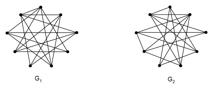
In XLSL , the $A_{\alpha}$-characteristics polynomial for all graphs on at most $10$ vertices have been enumerated. Also counted the number of graphs for which there exist at least one pair of non-isomorphic $\alpha$-Isospectral graphs. They get the smallest pair of non-isomorphic $\alpha$-Isospectral graphs with $9$ vertices, as an example see Figure(3).

Figure 3: Smallest pair of non-isomorphic $\alpha$-Isospectral graphs.

Using the above mentioned graphs, in Corollary(3.4),(4.4),(5.3) and Corollary(6.2) we get infinitely many non-isomorphic $\alpha$-Isospectral families of graphs.

99

References

• (1) Brouwer. A.E, and Haemers. W.H. Spectra of graphs. New York (NY): Springer, 2012.
• (2) Barik. S, Pati. S, and Sarma BK. The spectrum of the corona of two graphs. SIAM J. Discrete Math.2007;24:47-56.
• (3) Cvetkovc´´𝑐\acute{c}. D.M, Doob. M, Sachs. H. Spectra of graphs, theory and application. 3rd ed. Heidelberg, Johann Ambrosius Barth; 1995.
• (4) Cvetkovc´´𝑐\acute{c}. D.M, Rowlinson. P, Simi´´𝑖\acute{i}c. S. An introduction to the theory of graph spectra.Cambridge, Cambridge University Press; 2010.
• (5) Cui, S. Y. and Tian, G. X. The spectrum and the signless Laplacian spectrum of coronae, Linear Algebra Appl. 437,1692-1703 (2012).
• (6) Frucht, R. and Harary, F. On the corona of two graphs, Aequationes Math. 4,322-325 (1970).
• (7) Harary, F. Graph Theory, Addison-Wesley, Reading, MA, 1969.
• (8) Hou, Y. and Shiu, W. C. The spectrum of the edge corona of two graphs, Electron. J. Linear Algebra. 20 586-594 (2010).
• (9) Liu, X. and Liu, S. On the AΞ±subscript𝐴𝛼A_{\alpha}-characteristic polynomial of a graph, Linear Algebra Appl. 546, 274-288 (2018).
• (10) Lan, J. and Zhou, B. Spectra of graph operations based on R𝑅R-graph, Lin.Multilin. Alg. 63(7),1401-1422 (2015).
• (11) Liu. X, and Zhang Z. Spectra of subdivision-vertex and subdivision-edge joins of graphs, Linear Algebra Appl. 438,3547-3559 (2013).
• (12) Liu X, Zhou S. Spectra of the neighbourhood corona of two graphs. Linear Multilinear Algebra. 1205-1219(2013).
• (13) McLeman. C, and McNicholas E. Spectra of coronae. Linear Algebra Appl. 2011;435:998-1007.
• (14) Nikiforov, V. Merging the A- and Q- spectral theories, Appl.Anal. Discrete Math.11,81-107 (2017).
• (15) Wang. S, and Zhou. B. The signless Laplacian spectra of the corona and edge corona of two graphs.Linear Multilinear Algebra. 2013,61:197-204.