Eikonal solutions for moment hierarchies of Chemical Reaction Networks in the limits of large particle number

Abstract

Trajectory-based methods are well-developed to approximate steady-state probability distributions for stochastic processes in large-system limits. The trajectories are solutions to equations of motion of Hamiltonian dynamical systems, and are known as eikonals. They also express the leading flow lines along which probability currents balance. The existing eikonal methods for discrete-state processes including chemical reaction networks are based on the Liouville operator that evolves generating functions of the underlying probability distribution. We have previously derived Krishnamurthy:CRN_moments:17 ; Smith:CRN_moments:17 a representation for the generators of such processes that acts directly in the hierarchy of moments of the distribution, rather than on the distribution itself or on its generating function. We show here how in the large-system limit the steady-state condition for that generator reduces to a mapping from eikonals to the ratios of neighboring factorial moments, as a function of the order $k$ of these moments. The construction shows that the boundary values for the moment hierarchy, and thus its whole solution, are anchored in the interior fixed points of the Hamiltonian system, a result familiar from Freidlin-Wenztell theory. The direct derivation of eikonals from the moment representation further illustrates the relation between coherent-state and number fields in Doi-Peliti theory, clarifying the role of canonical transformations in that theory.
Keywords: Chemical Reaction Networks; Eikonal methods; Doi-Peliti theory.

I Introduction: directly solving for fluctuation moments in stochastic Chemical Reaction Networks

When solving for the steady states of stochastic processes, approximation methods are needed in all but the simplest cases. The choice of representation for the process and its generator can dictate the efficiency or comprehensibility of approximation methods that are available in that representation.

Two representations for the generators of stochastic processes that are now more than a century old vanKampen:Stoch_Proc:07 are the transition matrix of the master equation, acting directly on probability distributions, and the generator of the Liouville equation, acting on generating functions that are the Laplace transforms of those distributions.

A third representation can be constructed for the generator acting directly on the hierarchy of moments. For a class of discrete-state stochastic processes, we have obtained an explicit form for such a generator acting on the moment hierarchy Krishnamurthy:CRN_moments:17 ; Smith:CRN_moments:17 . These are the models of stochastic Chemical Reaction Networks (CRNs), which have been extensively studied Feinberg:def_01:87 ; Anderson:product_dist:10 ; Gunawardena:CRN_for_bio:03 ; Baez:QTRN_eq:14 ; Polettini:open_CNs_I:14 ; Polettini:diss_def:15 and are of both mathematical and practical interest. The moments of a probability distribution for a CRN arrange into a lattice with coordinates $k$, where $k$ is a vector whose components determine the moment of interest.

For CRNs with only finitely many reactions, the generator in the moment lattice takes the form of a discrete Laplacian, and is solved analogously to a heat equation. Because the dynamical equation for moments is linear, the steady-state condition can be reduced to a collection of constraints, one per lattice site. Time-invariance of the moment at index $k$ implies a constraint on the ratios of neighboring moments to the moment at $k$.

If a CRN has only one dynamical degree of freedom, a discrete Laplacian acting on its moments reduces to a recursion relation on the moment ratios. We showed in Krishnamurthy:CRN_moments:17 ; Smith:CRN_moments:17 that such recursions can be solved by a method of matched asymptotic expansions, in which low-order modes are solved recursively as one would expect, upward from the mean or variance, but high-order modes are solved (counterintuitively) by anchoring the moment ratios at large $k$, where they converge asymptotically to values set by parameters in the generator. For multivariate distributions, however, the corresponding method of solution encounters the difficulty faced in the solution of other Laplacian equations, which is the specification of boundary conditions. For the CRN moment hierarchies, the difficult boundaries are those on which one or more of the moments is not of asymptotically large order, since there is no approximation scheme which gives an estimate of such moments.

An alternative to direct solution of Laplacian equations, which addresses the problem of boundary conditions both computationally and conceptually, is the WKB method, which computes the leading exponential dependence of probability distributions in large-system limits. The key quantities in the WKB approximation are eikonals: locally least-improbable trajectories for improbable excursions, along which balance of probability currents determines the large-deviation behavior of the distribution. Eikonal solutions for stationary distributions, boundary values, and first-passage statistics of diffusion solutions in basins of attraction were extensively developed by Freidlin and Wentzell Freidlin:RPDS:98 . Related formulations in terms of 2-field functional integrals, for stochastic processes on discrete state spaces including those of CRNs, were derived by Doi and Peliti Doi:SecQuant:76 ; Doi:RDQFT:76 ; Peliti:PIBD:85 ; Peliti:AAZero:86 .

The stability properties of WKB methods are dual to those of the moment recursions in Krishnamurthy:CRN_moments:17 ; Smith:CRN_moments:17 , in that they propagate probability distributions outward into attenuating tails from the regions near the mean where probability is most concentrated. Those central regions are the main scale factors in the recursion approach, where matching conditions must be imposed between low and high moment orders. It is by grounding asymptotic regions in the centers of mass of probability distributions that WKB methods provide approximate solution methods for boundary-value problems Freidlin:RPDS:98 .

In this paper we derive the eikonal method to directly approximate the ratios of adjacent moments in the moment hierarchy. Our starting point will be the generator from Krishnamurthy:CRN_moments:17 ; Smith:CRN_moments:17 . The steady-state condition will reduce to a set of stationary-path equations that are the same as those for eikonals in Doi-Peliti theory. The new feature resulting from the moment representation is a mapping from the order $k$ of a moment to a specific position along the particular escape trajectory that governs the ratio of that moment to its local neighbors.

The analysis leads to three results: 1) The generator in the moment representation reduces in the large-system limit to the Liouville operator from the generating-function representation. 2) Boundary solutions for the WKB approximation are anchored on a discrete set of interior fixed points in the steady state, as they are in Freidlin-Wentzell theory. 3) The reduction of the generator from the moment representation to the Liouville operator clarifies the roles of number fields relative to coherent-state fields in Doi-Peliti theory, as these represent both activities and relative migration rates in steady states.

The presentation is organized as follows: Sec. II reviews three representations of the generator for a population process such as a CRN: the transition matrix of the master equation, the Liouville operator, and the generator in the moment representation. Sec. III derives the eikonal approximation for the moment hierarchies of CRNs. The large-number limit of the steady-state recursions of the moment hierarchy is derived, recovering the Liouville operator. It is then shown how the orders of the moments map to positions on the eikonals of the Liouville represenation. Sec. IV illustrates the eikonal construction on three example CRNs, beginning with a model that is exactly solvable to demonstrate convergence and show how finite-size effects are handled, and culminating in a model where eikonal methods are needed, but where they also break down in some regions due to trajectory crossing.

II Representations of the generator for discrete-state stochastic processes

To begin, we specify and introduce notation for the class of stochastic processes to be considered, and review the three representations of the generator. We will consider continuous-time Markov processes on discrete state spaces that are lattices of non-negative integers in some dimension $P$. Examples include a variety of population processes Smith:evo_games:15 , among which are stochastic CRNs described in more detail below.

States are indexed by vectors ${\rm n}\equiv\left[{{\rm n}}_{p}\right]$, in which $p\in 1,\ldots,P$ are called species and ${{\rm n}}_{p}$ is a non-negative integer giving the count (particles, individuals, etc.) of species $p$ in the population. Probability distributions over states ${\rm n}$ are denoted ${\rho}_{{\rm n}}$. A time-dependent probability evolves under a master equation of the form

$$\frac{d}{d\tau}{\rho}_{{\rm n}}=\sum_{{{\rm n}}^{\prime}}{\rm T}_{{\rm n}{{\rm n}}^{\prime}}{\rho}_{{{\rm n}}^{\prime}}.$$ (1)

${\rm T}_{{\rm n}{{\rm n}}^{\prime}}$ is a left-stochastic matrix called the transition matrix, and is one representation of the generator.

II.1 Moment-generating function and Liouville operator

The Laplace transform of a distribution ${\rho}_{{\rm n}}$ is called its moment-generating function (MGF). While the analytic structure of the Laplace transform is often a source of elegant solution methods and the reason to use the generating function Flajolet:anal_comb:09 , many problems require only its formal representation as a power series, and the ensuing linear algebra. For these, an abstract operator algebra such as that of Doi Doi:SecQuant:76 ; Doi:RDQFT:76 is more economical, especially for evaluating quadratures of Eq. (1). The Doi algebra is reviewed in numerous places Mattis:RDQFT:98 ; Kamenev:DP:02 ; Smith:LDP_SEA:11 ; Baez:QTRN:13 ; Baez:QTSM:17 , and we provide only a summary here.

Lowering operators $a_{p}$ that remove particles from a population state, and raising operators $a^{\dagger}_{q}$ that introduce particles, are defined by their commutation relation

$$\left[a_{p},a^{\dagger}_{q}\right]={\delta}_{pq},$$ (2)

where $p,q\in 1,\ldots,P$ and ${\delta}_{pq}$ is the Kronecker $\delta$ symbol.

Number states, corresponding to point distributions at each lattice index ${\rm n}$, are defined by the action of the lowering and raising operators on them, as

$$a_{p}\left|{\rm n}\right) ={{\rm n}}_{p}\left|{\rm n}-1_{p}\right) a^{\dagger}_{p}\left|{\rm n}\right) =\left|{\rm n}+1_{p}\right).$$ (3)

It follows that all number states can be built up from a ground state $\left|0\right)$ by multiplication with suitable powers of the $\left\{a^{\dagger}_{p}\right\}$.

The MGF of a distribution ${\rho}_{{\rm n}}$ is the sum of number states weighted by the coefficients of ${\rho}_{{\rm n}}$, denoted

$$\left|\phi\right)=\sum_{{\rm n}}{\rho}_{{\rm n}}\left|{\rm n}\right).$$ (4)

Eq. (1) implies a corresponding evolution equation for the MGF, known as the Liouville equation,

$$\frac{d}{d\tau}\left|\phi\right)=-\mathcal{L}\!\left(a^{\dagger},a\right)\left|\phi\right)$$ (5)

in which the Liouville operator $\mathcal{L}\!\left(a^{\dagger},a\right)$ is derived from the matrix of values ${\rm T}_{{\rm n}{{\rm n}}^{\prime}}$.

Computing the trace of a probability distribution is represented in the operator algebra in terms of an inner product with a dual state $\left(0\right|$ (which has the interpretation of a projection operator). Under an inner product called the Glauber norm,

$$\left(0\right|e^{\sum_{p}a_{p}}\left|{\rm n}\right)=1\;;\;\forall{\rm n},$$ (6)

in which all number states are normalized, the generating functions become vectors in a Hilbert space, completing the definition of the linear algebra. For some applications, including the Peliti functional integral introduced below, it remains useful to express the generating function as a function of a vector $z\equiv\left[z_{p}\right]$ of complex numbers. The analytic representation is extracted from the formal power series by the inner product

$$\left(0\right|e^{\sum_{p}z_{p}a_{p}}\left|\phi\right)=\phi\!\left(z\right).$$ (7)

II.1.1 Stochastic CRNs; the form of their Liouville operator

The subset of population processes that we will consider in detail are the stochastic CRNs. Each elementary event is an instance of some reaction, which removes one set of particles from the population and places another set of particles into it. The number of particles of each type that are removed or added give the stoichiometry of the reaction, and the rate of the reaction equals the probability for an instance to occur per unit time. Particles are sampled proportionally and without replacement, leading to mass-action kinetics at large numbers.

In a decomposition of CRNs due to Horn and Jackson Horn:mass_action:72 and Feinberg Feinberg:def_01:87 , the sets of particles either removed or created are called complexes. We denote the complexes that appear in a CRN with subscripts $i$, $j$; each reaction corresponds to a unique ordered pair $\left(ji\right)$ that removes complex $i$ and adds complex $j$.

The reaction network is specified by an adjacency matrix ${\mathbb{A}}_{\kappa}$ on the set of complexes, with the form

$${\mathbb{A}}_{\kappa}\equiv\sum_{\left(i,j\right)}\left(w_{j}-w_{i}\right){\kappa}_{ji}w_{i}^{T}.$$ (8)

$w_{i}$, a column vector, is an indicator function with 1 in the $i$th position and zero elsewhere; $w_{i}^{T}$ is its transpose. ${\kappa}_{ji}$ is the reaction rate constant for reaction $\left(ji\right)$, with respect to units $d\tau$ for time. ${\mathbb{A}}_{\kappa}$ is left-stochastic on complexes, as ${\rm T}_{{\rm n}{{\rm n}}^{\prime}}$ is on states.

The matrix ${\mathbb{A}}_{\kappa}$ acts to the right on a column vector of activities for complexes. These activities are extracted from a state $\left|\phi\right)$ by a vector ${\psi}_{Y}\equiv\left[{\psi}_{Y}^{i}\right]$ in which the components are the operators

$${\psi}_{Y}^{i}\!\left(a\right)\equiv\prod_{p}a_{p}^{y^{i}_{p}}$$ (9)

$Y\equiv\left[y^{i}_{p}\right]$ is the matrix of stoichiometric components, giving the counts of species $p$ in each complex $i$.

The rate equation for the CRN defined by ${\mathbb{A}}_{\kappa}$ and $Y$ can be written in the form

$$\frac{dn}{d\tau}=Y{\mathbb{A}}_{\kappa}{\psi}_{Y}\!\left(n\right)$$ (10)

Here $n$ is a vector that corresponds in the mean-field approximation to the vector of expectations $\left<{\rm n}\right>\equiv\sum_{{\rm n}}{\rm n}{\rho}_{{\rm n}}$.

As we show in Krishnamurthy:CRN_moments:17 ; Smith:CRN_moments:17 , the Liouville operator for this class of CRNs takes the compact form

$$-\mathcal{L}\!\left(a^{\dagger},a\right)={\psi}^{T}_{Y}\!\left(a^{\dagger}\right){\mathbb{A}}_{\kappa}\,{\psi}_{Y}\!\left(a\right)$$ (11)

The exact equation for the time evolution of all moments in the distribution ${\rho}_{{\rm n}}$, follows from this form and from the commutation relations (2).

II.1.2 The Doi-Peliti functional integral and its action functional

Peliti Peliti:PIBD:85 ; Peliti:AAZero:86 introduced a path-integral representation for the quadrature of the Liouville equation (5) based on an expansion in coherent states. For $\xi\equiv\left[{\xi}_{p}\right]$ a vector of complex coefficients, the coherent state

$$\left|\xi\right)\equiv e^{\left(a^{\dagger}-1\right)\xi}\left|0\right)$$ (12)

is an eigenstate of the lowering operators, with eigenvalues

$$a_{p}\left|\xi\right)={\xi}_{p}\left|\xi\right).$$ (13)

In Eq. (12) we introduce a convention that $a^{\dagger}$ is a row vector, $\xi$ is a column vector, and $a^{\dagger}\xi$ is the vector inner product of the two.

Through constructions that are now standard Smith:LDP_SEA:11 ; Krishnamurthy:CRN_moments:17 ; Smith:CRN_moments:17 , the time-dependent solution to Eq. (5), converted to complex arguments by Eq. (7), may be written as the 2-field functional integral

$${\phi}_{T}\!\left(z\right)=\int_{0}^{T}\mathcal{D}{\xi}^{\dagger}\mathcal{D}{\xi}e^{\left(z-{{\xi}^{\dagger}}_{T}\right){\xi}_{T}}e^{-S}{\phi}_{0}\!\left({\xi}_{0}^{\dagger}\right).$$ (14)

${\xi}^{\dagger}$ and $\xi$ are now histories indexed by time $\tau\in\left[0,T\right]$. ${\phi}_{0}$ is the generating function for the initial distribution at $\tau=0$, and ${\phi}_{T}$ is its image evolved to $\tau=T$.

All influence from the CRN dynamics in the integral (14) comes through the action functional

$$S=\int_{0}^{T}d\tau\left\{-\left(d_{\tau}{\xi}^{\dagger}\right)\xi+\mathcal{L}\!\left({\xi}^{\dagger},\xi\right)\right\}.$$ (15)

$\xi$ appears as a coordinate variable, ${\xi}^{\dagger}$ is its conjugate momentum, and the place of the Hamiltonian is filled by the Liouville function $\mathcal{L}$ in which $\xi$ takes the place of operator $a$ and ${\xi}^{\dagger}$ takes the place of $a^{\dagger}$. For the generator class (11) of CRNs, we have

$$-\mathcal{L}\!\left({\xi}^{\dagger},\xi\right)={\psi}^{T}_{Y}\!\left({\xi}^{\dagger}\right){\mathbb{A}}_{\kappa}\,{\psi}_{Y}\!\left(\xi\right).$$ (16)

II.1.3 Canonical transformations: coherent-state and number-potential coordinates

In terms of the coherent states used to construct the functional integral (14), the components of the number index ${\rm n}$ correspond to a bilinear form $n_{p}={\xi}^{\dagger}_{p}{\xi}_{p}$. The number field may be made an elementary degree of freedom as part of a canonical transformation Goldstein:ClassMech:01 of the coordinates of the Hamiltonian dynamical system,

$${\xi}_{p}^{\dagger} \equiv e^{{\eta}_{p}} {\xi}_{p} \equiv e^{-{\eta}_{p}}n_{p}.$$ (17)

$\eta$, the conjugate momentum to the number coordinate, admits a variety of interpretations. In the construction of the equilibrium free energy of a chemical mixture, it has the dimensions of a chemical potential Smith:LDP_SEA:11 , so we will refer to $\left(\eta,n\right)$ as number-potential coordinates. Both $\xi$ and $n$ have dimensions of species numbers, and one of the subtleties of Doi-Peliti theory is understanding the difference of their meaning in WKB-type approximations. The eikonal approximation for moment ratios is interesting because it establishes a relation between the two in the same observable.

The Doi-Peliti integral in number-potential coordinates becomes

$${\phi}_{T}\!\left(z\right)=\int_{0}^{T}\mathcal{D}\eta\mathcal{D}ne^{\left(ze^{-{\eta}_{T}}-1\right)n_{T}}e^{-S}{\phi}_{0}\!\left(e^{{\eta}_{0}}\right),$$ (18)

in which the action is

$$S=\int_{0}^{T}d\tau\left\{-\left(d_{\tau}\eta\right)n+\mathcal{L}\!\left(\eta,n\right)\right\}.$$ (19)

Preservation of the form of the kinetic term as $-\left(d_{\tau}{\xi}^{\dagger}\right)\xi=-\left(d_{\tau}\eta\right)n$ ensures that Eq. (18) is canonical. The Liouville function $\mathcal{L}\!\left(\eta,n\right)$ is the same as $\mathcal{L}\!\left({\xi}^{\dagger},\xi\right)$ in Eq. (15) evaluated in the transformed variables.

II.2 Moment hierarchy and its generator

For CRNs with mass action rates, the macroscopic expression of proportional sampling without replacement at the microscale, the moments that have a simple behavior are neither ordinary moments nor cumulants, but rather the expectations of falling factorials Baez:QTRN:13 , which we term factorial moments. A compact notation for the falling factorial of number $n_{p}$ at order $k_{p}$ is

$${{\rm n}}_{p}^{\underline{k_{p}}} \equiv\frac{{{\rm n}}_{p}!}{\left({{\rm n}}_{p}-k_{p}\right)!} ;\;k_{p}\leq{{\rm n}}_{p}$$

$$\equiv 0 ;\;k_{p}>{{\rm n}}_{p}.$$ (20)

In a CRN, the activity products corresponding to the complexes $i$ in a state ${\rm n}$ make up a column vector that we denote ${\Psi}_{Y}\equiv\left[{\Psi}_{Y}^{i}\right]$ with

$${\Psi}_{Y}^{i}\!\left({\rm n}\right)\equiv\prod_{p}{{\rm n}}_{p}^{\underline{y_{p}^{i}}}$$ (21)

In the Liouville equation (5), the complex-lowering operators ${\psi}_{Y}^{i}$ from Eq. (9) act respectively on number states and coherent states as

$${\psi}_{Y}^{i}\!\left(a\right)\left|{\rm n}\right) ={\Psi}_{Y}^{i}\!\left({\rm n}\right)\left|{\rm n}-y^{i}\right)$$

$${\psi}_{Y}^{i}\!\left(a\right)\left|\xi\right) ={\psi}_{Y}^{i}\!\left(\xi\right)\left|\xi\right).$$ (22)

Finally, in parallel to the designation $\phi\!\left(z\right)$ from Eq. (7) for the MGF, we denote the lattice of factorial moments $\Phi\equiv\left[{\Phi}_{k}\right]$ with

$${\Phi}_{k}\equiv\left<\prod_{p}{{\rm n}}_{p}^{\underline{k_{p}}}\right>.$$ (23)

We showed in Krishnamurthy:CRN_moments:17 ; Smith:CRN_moments:17 that the Liouville equation (5), used to evolve the probability distribution defining the average in Eq. (23), implies the equation of motion for the moment hierarchy

$$\frac{d}{d\tau}{\Phi}_{k}=\dot{\prod_{p}}\left[\sum_{j_{p}=0}^{k_{p}}\left(\begin{array}[]{c}k_{p}\\ j_{p}\end{array}\right)Y_{p}^{\underline{j_{p}}}\,e^{{\left(k-j\right)}_{p}\,\partial/\partial Y_{p}}\right]{\mathbb{A}}_{\kappa}\left<{\Psi}_{Y}\!\left({\rm n}\right)\right>$$ (26)

$$=\sum_{j_{1}=0}^{k_{1}}\left(\begin{array}[]{c}k_{1}\\ j_{1}\end{array}\right)\ldots\sum_{j_{P}=0}^{k_{P}}\left(\begin{array}[]{c}k_{P}\\ j_{P}\end{array}\right)\left[\dot{\prod_{p}}Y_{p}^{\underline{j_{p}}}\,\right]{\mathbb{A}}_{\kappa}\left<{\Psi}_{Y+\left(k-j\right)}\!\left({\rm n}\right)\right>$$ (31)

$$\equiv\sum_{k^{\prime}}{\Lambda}_{kk^{\prime}}{\Phi}_{k^{\prime}}.$$ (32)

The notation ${\dot{\prod}}_{p}$ stands for a product of terms over the species index $p$ that is performed within each component of a row vector over complexes $i$. $Y_{p}\equiv\left[y_{p}^{i}\right]$ is the row vector of stoichiometric coefficients for species $p$ in each complex, and both factorials $Y_{p}^{\underline{j_{p}}}$ and integer shift operators $e^{{\left(k-j\right)}_{p}\,\partial/\partial Y_{p}}$ are evaluated component-wise in indices $i$. The resulting row vector is contracted on the left with ${\mathbb{A}}_{\kappa}$. The matrix $\Lambda\equiv\left[{\Lambda}_{kk^{\prime}}\right]$ is the representation of the generator acting on the moment hierarchy.

III The eikonal approximation for the moment hierarchy

Eikonal approximations for the probability distribution ${\rho}_{{\rm n}}$, in steady state, are based on a leading-exponential expansion ${\rho}_{{\rm n}}\sim e^{-\Xi\left({\rm n}\right)}$ expressing the large-deviation scaling. In Section III.2.2, we demonstrate how this approximation for the steady-state probability distribution results in a corresponding approximation for the factorial moments. We show first however that this approximation for the factorial moments, in a large-number limit in steady state, may be arrived at directly from the moment hierarchy as well.

The factorial moments Eq. (32), under the steady state condition, satisfy a hierarchy of relations $0=\sum_{k^{\prime}}{\Lambda}_{kk^{\prime}}{\Phi}_{k^{\prime}}$ By dividing through by ${\Phi}_{k}$, each of these may be written as a constraint on ratios of neighboring moments ${\Phi}_{k^{\prime}}$ to ${\Phi}_{k}$. In one dimension (for CRN’s involving only one species) these become recursion relations, which may be solved by a method of matched asymptotic expansions Krishnamurthy:CRN_moments:17 ; Smith:CRN_moments:17 downward from $k\rightarrow\infty$ and upward from $k=0$.

It will not be surprising that the steady-state condition is equivalent to a condition $\mathcal{L}=0$ in the Liouville representation, a relation suggested by Eq. (5). We show in the following that the steady-state condition for moments reduces in the large-system limit to a particular form of the condition $\mathcal{L}=0$ equivalent to the coherent-state expression in the action (15). However, as is well known in the literature on momentum-space WKB methods Dykman:chem_paths:94 ; Assaf:mom_WKB:17 , the $\mathcal{L}=0$ submanifold contains “momentum” values (our potential field $\eta$) consistent with derivatives of many different distributions. To isolate the stationary distribution requires additional information from boundary conditions; which is the problem that makes direct solution of higher-dimensional moment equations difficult. What is gained in passing to the continuum limit is a non-local relation of the momentum values at each point through stationary trajectories under variation of the action (15) anchored in the classical fixed points of the rate equation, a result developed extensively for the solution of boundary value and first-passage problems by Freidlin and Wentzell Freidlin:RPDS:98 , and since generalized to many classes of stochastic processes Dykman:chem_paths:94 ; Assaf:mom_WKB:17 .

III.1 Large-number limit of the generator in the moment representation

The counterpart to a continuum limit in the moment hierarchy comes from the observation that, if both particle numbers and the orders of moments are large, the ratios of factorial moments at adjacent $k$ indices should change slowly with $k$. If that is the case, then factorial moments offset by finite lattice shifts will be related through one ratio of moments in each direction $p$, raised to powers. For the offset term appearing in Eq. (32), that limiting behavior becomes

$$\left<{\Psi}_{Y+\left(k-j\right)}^{i}\!\left({\rm n}\right)\right> \underset{n\gg 1}{\rightarrow}{\left.\left(\prod_{p}R_{p}^{y^{i}_{p}-j_{p}}\right)\right|}_{k}\left<\prod_{p}{{\rm n}}_{p}^{\underline{k_{p}}}\right>$$

$$={\left.{\psi}_{Y-j}^{i}\!\left(R\right)\right|}_{k}{\Phi}_{k}.$$ (33)

Here ${\left.R_{p}\right|}_{k}$ denotes $\left<{{\rm n}}^{\underline{k+1_{p}}}\right>/\left<{{\rm n}}^{\underline{k}}\right>$: the ratio of factorial moments incremented by the $p$th component of $k$, in a neighborhood of the index $k$ of the reference moment ${\Phi}_{k}$. $R\equiv\left[R_{p}\right]$ is the vector with these components at any $k$. The product of powers of $R_{p}$ in Eq. (33) will be independent of the walk on the lattice between $k$ and $k+Y-j$, and at large $k$ corrections from the exact matrices ${\Lambda}_{kk^{\prime}}$ will scale as $\mathcal{O}\!\left(1/k\right)$ or smaller.

Dividing Eq. (32) through by ${\Phi}_{k}$ and then taking the steady-state condition, produces the sum

$$0 =\dot{\prod_{p}}\left[\sum_{j_{p}=0}^{k_{p}}\left(\begin{array}[]{c}k_{p}\\ j_{p}\end{array}\right)Y_{p}^{\underline{j_{p}}}\,e^{-j_{p}\,\partial/\partial Y_{p}}\right]{\mathbb{A}}_{\kappa}{\left.{\psi}_{Y}\!\left(R\right)\right|}_{k}$$ (36)

$$=\sum_{j_{1}=0}^{k_{1}}\left(\begin{array}[]{c}k_{1}\\ j_{1}\end{array}\right)\ldots\sum_{j_{P}=0}^{k_{P}}\left(\begin{array}[]{c}k_{P}\\ j_{P}\end{array}\right)\left[\dot{\prod_{p}}Y_{p}^{\underline{j_{p}}}\,\right]{\mathbb{A}}_{\kappa}{\left.{\psi}_{Y-j}\!\left(R\right)\right|}_{k}$$ (41)

$$=\sum_{j_{1}=0}^{k_{1}}k_{1}^{\underline{j_{1}}}\ldots\sum_{j_{P}=0}^{k_{P}}k_{P}^{\underline{j_{P}}}\left[\dot{\prod_{p}}\left(\begin{array}[]{c}Y_{p}\\ j_{p}\end{array}\right)\right]e^{-j\cdot\partial/\partial Y}{\mathbb{A}}_{\kappa}{\left.{\psi}_{Y}\!\left(R\right)\right|}_{k}$$ (44)

$$=\dot{\prod_{p}}\left[\sum_{j_{p}=0}^{k_{p}}\left(\begin{array}[]{c}Y_{p}\\ j_{p}\end{array}\right)k_{p}^{\underline{j_{p}}}e^{-j_{p}\,\partial/\partial Y_{p}}\right]{\mathbb{A}}_{\kappa}{\left.{\psi}_{Y}\!\left(R\right)\right|}_{k}$$ (47)

The coefficient in the row vector on the third line of Eq. (47) at index $i$ is the product of binomial coefficients

$$\prod_{p}\left(\begin{array}[]{c}y^{i}_{p}\\ j_{p}\end{array}\right)$$

for $j_{p}\leq y^{i}_{p}$ and zero otherwise. If $k_{p}$ are large while $j_{p}$ remain bounded by fixed $y^{i}_{p}$, up to corrections of order $1/k_{p}$ we may approximate $k_{p}^{\underline{j_{p}}}\approx k_{p}^{j_{p}}$. Then the sum on $j_{p}$ reduces back to

$$0={\psi}^{T}_{Y}\!\left(1+ke^{-\partial/\partial Y}\right){\mathbb{A}}_{\kappa}{\left.{\psi}_{Y}\!\left(R\right)\right|}_{k},$$ (48)

recognizable as the CRN Liouville operator from Eq. (11). (As elsewhere, the argument $1+ke^{-\partial/\partial Y}$ is to be understood as a vector with components $1+k_{p}e^{-\partial/\partial Y_{p}}$ taking the place of $a^{\dagger}_{p}$.)

The operator $e^{-\partial/\partial Y_{p}}$, acting on functions ${\psi}^{i}_{Y}\!\left(R\right)$ has the effect of reducing any such product by one factor of $R_{p}$. Thus we can rewrite the expression (48) as

$$0={\psi}^{T}_{Y}\!\left(1+k/R\right){\mathbb{A}}_{\kappa}{\left.{\psi}_{Y}\!\left(R\right)\right|}_{k}.$$ (49)

Vanishing of $\Lambda\Phi$ in Eq. (33) is thus the same in the large-number limit as vanishing of the Liouville operator in the steady-state condition (5) for the generating function, with numbers $R$ replacing the operator $a$ and numbers $1+k/R$ replacing the operator $a^{\dagger}$.

III.2 Connection to the standard eikonal approximation

III.2.1 Preliminaries: stationary-path approximations in Doi-Peliti theory, and the source of boundary conditions for the steady state

The Peliti construction Peliti:PIBD:85 ; Peliti:AAZero:86 likewise replaces $a^{\dagger}$ and $a$ in $\mathcal{L}$ with the coherent-state parameters that are their eigenvalues. Stationary trajectories arise in the saddle-point approximation of the functional integral (14), where they are solutions to the vanishing of the variational derivative of $S$. These stationary paths are those which provide the eikonal approximation to the probability density and $\mathcal{L}\!\left({\xi}^{\dagger},\xi\right)=0$ is a property of these paths.

The equations of motion from the variation of $S$ in Eq. (15) are

$$\frac{d\xi}{d\tau} =-\frac{\partial\mathcal{L}}{\partial{\xi}^{\dagger}} \frac{d{\xi}^{\dagger}}{d\tau} =\frac{\partial\mathcal{L}}{\partial\xi}.$$ (50)

For the action (19) in number-potential fields, the equivalent forms are:

$$\frac{dn}{d\tau} =-\frac{\partial\mathcal{L}}{\partial\eta} \frac{d\eta}{d\tau} =\frac{\partial\mathcal{L}}{\partial n}.$$ (51)

Solutions with ${\xi}^{\dagger}\equiv 1$ or $\eta\equiv 0$ reproduce the mean-field rate equations (10) for $n$, which then coincides with $\xi$.

Potential solutions for $R$ joint with $1+k/R$ come from points along trajectories with ${\xi}^{\dagger}>1$, describing improbable excursions, for which $n\neq\xi$. If the dimension of the subspace of dynamical degrees of freedom in a CRN is some number $s\leq P$, the space of tangent vectors to stationary trajectories through a point has dimension $2s$, and $\mathcal{L}=0$ specifies a $\left(2s-1\right)$-dimensional manifold of possible solutions.

The saddle-point approximation (denoted $\sim$) to the value of the generating function (18) is the integral over an eikonal

$${\phi}_{T}\!\left(z\right) \sim{\left.\left(\prod_{p}z_{p}^{{{\rm n}}_{p}}\right){\rho}_{{\rm n}}\right|}_{{\rm n}={\bar{n}}_{T}}\sim e^{\int_{0}^{T}d\tau\left(d_{\tau}\bar{\eta}\right)\bar{n}},$$ (52)

where the trajectory $\left({\bar{\eta}}_{\tau},{\bar{n}}_{\tau}\right)$ satisfies equations (51) and has terminal conditions for $\bar{\eta}$ derived from the variation of $n_{T}$, and initial conditions for $\bar{n}$ derived from variation of ${\eta}_{0}$ including the contribution to the initial-value function ${\phi}_{0}\!\left(e^{{\eta}_{0}}\right)$.

For the steady-state distribution, $T\rightarrow\infty$ and any trajectory from the initial conditions passes arbitrarily close to one of the attracting fixed points and remains there arbitrarily long before escaping to the final values $\left({\bar{\eta}}_{T},{\bar{n}}_{T}\right)$. Therefore the relevant eikonals are the escape trajectories from the attracting fixed points of the rate equation  (10), with initial values ${\eta}_{0}=0$ from the converging solutions, and final values ${\bar{\eta}}_{T}$ determined by $z$.

The distribution is then obtained from the Legendre transform of the cumulant-generating function $\log{\phi}_{T}\!\left(z\right)$. Choosing a value $z$ for which ${\bar{n}}_{T}={\rm n}$, and subtracting ${\bar{n}}_{T}\log z$, subtracts a total derivative of $\bar{\eta}\,\bar{n}$ from the integral in Eq. (52), leaving

$${\rho}_{{\rm n}} \sim e^{-\int^{{\rm n}}\bar{\eta}\,d\bar{n}}\equiv e^{-\Xi\left({\rm n}\right)}.$$ (53)

In Eq. (53) we introduce the effective potential $\Xi\left({\rm n}\right)$ defined as the eikonal integral

$$\Xi\!\left({\rm n}\right)\equiv\int^{T}d\tau\,\bar{\eta}\,d_{\tau}\bar{n}=\int^{{\rm n}}\bar{\eta}\,d\bar{n}.$$ (54)

III.2.2 Large-deviations scaling and saddle-point approximation of factorial moments

The leading exponential dependence captured by the eikonal integral gives the system’s large-deviations scaling Ellis:ELDSM:85 if, when we descale number ${\rm n}$ by some characteristic scale $n_{C}$ as

$$\frac{{\rm n}}{n_{C}}\equiv x,$$ (55)

and let $n_{C}$ become large, stationary properties such as trajectories $\left(\bar{\eta},\bar{n}/n_{C}\right)$ become asymptotically independent of $n_{C}$. In that case the effective potential separates into scale and structure components Touchette:large_dev:09 as

$$\Xi\!\left({\rm n}\right) =n_{C}\int^{{\rm n}}\bar{\eta}\,d\left(\bar{n}/n_{C}\right)\equiv n_{C}\int^{x}\bar{\eta}\,d\bar{x}\equiv n_{C}\hat{\Xi}\!\left(x\right).$$ (56)

$\hat{\Xi}\!\left(x\right)$ is called the rate function of the large-deviations approximation for ${\rho}_{{\rm n}}$.

From the large-deviations approximation to ${\rho}_{{\rm n}}$, the factorial moment at order $k$ has an implied approximation

$$\left<{{\rm n}}^{\underline{k}}\right> \sim\int dxn_{C}e^{-n_{C}\hat{\Xi}\!\left(x\right)}\frac{\left(n_{C}x\right)!}{\left(n_{C}x-n_{C}y\right)!}$$

$$\approx n_{C}^{k}\int dxn_{C}e^{-n_{C}\hat{\Xi}\left(x\right)}e^{n_{C}\left\{x\left[\log x-1\right]-\left(x-y\right)\left[\log\left(x-y\right)-1\right]\right\}},$$ (57)

where we have defined $y\equiv k/n_{C}$ in parallel with Eq. (55). $\sim$ in the first line of Eq. (57) denotes the saddle-point approximation to the effective potential, while $\approx$ in the second line indicates the Stirling approximation for factorials.

The scale factor $n_{C}$ in Eq. (57) separates from a rate function including the contribution from the falling factorials, which we therefore denote

$$\mathbf{\hat{\Xi}}\!\left(x;y\right) =\hat{\Xi}\!\left(x\right)+\left(x-y\right)\left[\log\left(x-y\right)-1\right]-x\left[\log x-1\right]$$ (58)

A second saddle-point approximation in the integral yields an expression for the descaled factorial moment as a finite sum

$${\hat{\Phi}}_{k}\equiv\frac{\left<{{\rm n}}^{\underline{k}}\right>}{n_{C}^{k}}\sim\sum_{\bar{x}\left(y\right)}e^{-n_{C}\mathbf{\hat{\Xi}}\left(\bar{x};y\right)},$$ (59)

where the saddle points $\bar{x}\!\left(y\right)$ are any solutions to the equation

$$\log\left(\frac{{\bar{x}}_{p}}{{\bar{x}}_{p}-y_{p}}\right)={\left.\frac{d\hat{\Xi}}{dx_{p}}\right|}_{\bar{x}}={\eta}_{p}\!\left(\bar{x}\right).$$ (60)

The ratio of two such solutions at values of $k$ separated by $1_{p}$ produces an expression for descaled moment ratios from Eq. (33) as

$${\left.{\hat{R}}_{p}\right|}_{y}\equiv\frac{{\left.R_{p}\right|}_{k}}{n_{C}}=\frac{\left<{{\rm n}}^{\underline{k+1_{p}}}\right>/\left<{{\rm n}}^{\underline{k}}\right>}{n_{C}}$$

$$\underset{n_{C}\rightarrow\infty}{\rightarrow}\exp\left\{\frac{d}{dy_{p}}\mathbf{\hat{\Xi}}\!\left(\bar{x};y\right)\right\}$$

$$=\exp\left\{\log\left({\bar{x}}_{p}-y_{p}\right)+\frac{{d\bar{x}}_{p}}{dy_{p}}{\left[\log\left(\frac{x_{p}}{x_{p}-y_{p}}\right)-\frac{d\hat{\Xi}}{dx_{p}}\right]}_{x=\bar{x}}\right\}$$

$$={\bar{x}}_{p}-y_{p}.$$ (61)

From the saddle-point condition (60) and the expression (61) for $\hat{R}$ it follows that

$$y_{p} ={\bar{x}}_{p}\left(1-e^{-{\eta}_{p}}\right)$$

$$\frac{{\hat{R}}_{p}}{{\bar{x}}_{p}} =\frac{{\bar{x}}_{p}-y_{p}}{{\bar{x}}_{p}}=e^{-{\eta}_{p}}.$$ (62)

Together with the definition of field variables (17) we confirm that ${\hat{R}}_{p}$ corresponds to the descaled coherent-state field ${\hat{\xi}}_{p}\equiv{\xi}_{p}/n_{C}$. Some algebra then gives

$$1+\frac{k_{p}}{R_{p}} =\frac{{\hat{R}}_{p}+y_{p}}{{\hat{R}}_{p}}=\frac{{\bar{x}}_{p}}{{\hat{R}}_{p}}=e^{{\eta}_{p}}$$ (63)

confirming that $1+k/R$ corresponds to ${\xi}^{\dagger}$, consistent with Eq. (49). Eq. (61) and Eq. (60) hence directly give us a non-trivial approximation for the factorial moment ratios, consistent with the eikonal approximation for the probability distribution.

III.2.3 Direct derivation from the definitions of factorial moments

The mappings (62,63) can be obtained directly from the definitions of factorial moments. The second line in Eq. (62) is equivalent to

$$\bar{\xi}=\bar{n}-k.$$ (64)

The relations (22) between actions of the lowering operator give

$${\bar{\xi}}_{p}=\frac{\left<{{\rm n}}^{\underline{k+1_{p}}}\right>}{\left<{{\rm n}}^{\underline{k}}\right>}.$$ (65)

Then, from the definition (20),

$${{\rm n}}^{\underline{k+1_{p}}}={{\rm n}}^{\underline{k}}\left(n_{p}-k_{p}\right),$$ (66)

Eq. (64) is nothing more than the large-number-limiting relation

$$\frac{\left<{{\rm n}}^{\underline{k}}{\rm n}\right>}{\left<{{\rm n}}^{\underline{k}}\right>}=\left<{\rm n}\right>.$$ (67)

In the background of a factorial moment, taking the expectation of an additional factor of $n$ results in just the mean-field value to $\mathcal{O}\!\left(n^{0}\right)$.

The identification of Eq. (49) as $\mathcal{L}\!\left({\xi}^{\dagger},\xi\right)$ along stationary trajectories is thus confirmed, along with a map from $y=k/n_{C}$ to the position $\bar{x}$ on the trajectory that controls the corresponding moment ratio $\hat{R}$. The mapping depends on convexity of the effective potential $\Xi$. If $\Xi$ is only locally convex, as occurs in systems with multiple metastable fixed points, then $\hat{R}$ is assigned to a stable branch by a rule equivalent to a coexistence condition. We provide examples in Sec. IV.

IV Examples

A brief treatment will be given of three CRN examples, with complexity added at each stage to illustrate the uses, variants, and limitations of eikonal solutions. The first example is a 1-species autocatalytic system, illustrating the handling of bistability. Methods are introduced to characterize large-$n_{C}$ convergence of the eikonal approximation and to estimate finite-size corrections. The second example is a symmetric 2-species cross-catalytic system that reproduces the fixed-point structure of the 1-dimensional model along its axis of symmetry, and introduces a boundary-value problem that is difficult to solve without eikonal methods. The third example is a 2-species CRN known as the Selkov model, which may be given a fixed-point structure similar to the previous cases, but lacks axes of symmetry.

Closed-form solution of the 1-dimensional CRN emphasizes why the Hamilton-Jacobi dual coordinates $n$ and $\eta$ are also the index and log-derivative of the stationary distribution, with $e^{\eta}$ representing a ratio of transport rates for probability current upward and downward in $n$. In higher dimensions where closed-form solutions are no longer available, the stationarity condition under the action (15) ensures that the planes normal to $\eta$ remain isoclines of the steady-state probability, so that the interpretation of current balance remains as in the 1-dimensional case.

In the symmetric cross-catalytic model, values of the effective potential at the fixed points may be computed directly from the recursion relations, without solving for eikonals. In the final model without symmetry, eikonal methods are required to estimate the relative residence times at fixed points, but they may also exhibit caustics and other regions where the eikonal approximation breaks down.

IV.1 Exactly solvable 1-variable autocatalytic CRN: multiple fixed points and finite-size scaling

Fig. 1 shows a 1-species autocatalytic CRN, which for suitable parameters possesses two metastable states, expressed as two stable fixed points of the mean-field equations (10). The bipartite graphical notation in the figure represents the decomposition of CRNs due to Horn and Jackson Horn:mass_action:72 and Feinberg Feinberg:def_01:87 , and is elaborated in detail in Krishnamurthy:CRN_moments:17 ; Smith:CRN_moments:17 .

Figure 1: A network with one species and four complexes, which supports two metastable states at some values of the rate constants. Filled circles are species; open circles are complexes. Dashed lines between complexes indicate (directed) reactions; solid lines from species to complexes reflect the stoichiometric coefficients of the CRN.

The recursion relations for this model were considered in detail in Smith:CRN_moments:17 , where they were solved by methods of matched asymptotic expansions and validated against Gillespie simulations. Here we use the model to illustrate the relation between the moment and Liouville representations and to consider finite-size deviations from the eikonal approximation. Additional detail is given in App. A.

The reaction schema corresponding to Fig. 1 is

$$\varnothing \xrightleftharpoons[k_{2}]{\epsilon}{\rm A} 2{\rm A} \xrightleftharpoons[{\bar{k}}_{1}]{k_{1}}3{\rm A}.$$ (68)

where $A$ is the species name, and $\epsilon$, $k_{2}$, $k_{1}$, and ${\bar{k}}_{i}$ are reaction rate constants. $\varnothing$ indicates the null species, which may stand for buffered external species for which fluctuations are not considered, or depending on the context, on de novo creation or annihilation of particles. The mean-field equation of motion (10) for the number $n$ of $A$ particles in the system is

$$\frac{dn}{d\tau}=\epsilon-k_{2}n+k_{1}{n}^{2}-{\bar{k}}_{1}{n}^{3}.$$ (69)

The exact recursion relation for $R_{k}$ following from Eq. (32) was shown in Smith:CRN_moments:17 to be

$$R_{k}=\frac{\epsilon+\left(k-1\right)\left(k-2\right)k_{1}}{k_{2}-k_{1}R_{k+1}+{\bar{k}}_{1}R_{k+2}R_{k+1}-\left(k-1\right)\left(2k_{1}-2{\bar{k}}_{1}R_{k+1}\right)+{\bar{k}}_{1}\left(k-1\right)\left(k-2\right)}.$$ (70)

Descaled variables to extract the large-deviations system behavior will be denoted

$$\epsilon =\varepsilon n_{C} k_{2} ={\kappa}_{2}$$

$$k_{1} ={\kappa}_{1}/n_{C} {\bar{k}}_{1} ={\bar{\kappa}}_{1}/n_{C}^{2}$$

$$n \equiv xn_{C} R \equiv\hat{R}n_{C}$$

$$k \equiv yn_{C} \mathcal{L} =\hat{\mathcal{L}}n_{C}.$$ (71)

In terms of these Eq. (70) has the large-$n_{C}$ and large-$k$ limit

$$\hat{R}=\frac{\varepsilon+y^{2}{\kappa}_{1}}{{\kappa}_{2}-{\kappa}_{1}\hat{R}+{\bar{\kappa}}_{1}{\hat{R}}^{2}-2y\left({\kappa}_{1}-{\bar{\kappa}}_{1}\hat{R}\right)+{\bar{\kappa}}_{1}y^{2}}.$$ (72)

Non-negative real solutions to

$$y=\sqrt{\frac{{\kappa}_{2}\hat{R}-\varepsilon}{{\kappa}_{1}-{\bar{\kappa}}_{1}\hat{R}}}-\hat{R}$$ (73)

give the two branches of $\hat{R}\!\left(y\right)$ satisfying Eq. (72).

The Liouville function in number-potential fields, derived following standard methods (see Smith:LDP_SEA:11 ; Krishnamurthy:CRN_moments:17 ; Smith:CRN_moments:17 ), is

$$\hat{\mathcal{L}} =\left(1-e^{\eta}\right)\left(\varepsilon+{\kappa}_{1}x^{2}\right)+\left(1-e^{-\eta}\right)\left({\kappa}_{2}+{\bar{\kappa}}_{1}x^{2}\right)x.$$ (74)

It is immediate to check that under the assignments (62), Eq. (72) re-arranges to

$$0 =-\varepsilon+{\kappa}_{2}\hat{R}-{\left(y+\hat{R}\right)}^{2}\left({\kappa}_{1}-{\bar{\kappa}}_{1}\hat{R}\right)=\frac{\hat{R}}{y}\hat{\mathcal{L}}.$$ (75)

For a 1-dimensional system, the condition $\mathcal{L}=0$ is sufficient to solve jointly for $x$ and $\eta$, giving a relation

$$\hat{R}=\frac{\varepsilon+{\kappa}_{1}x^{2}}{{\kappa}_{2}+{\bar{\kappa}}_{1}x^{2}}$$ (76)

that is equivalent under the mapping (62) to Eq. (73). It follows also that escape trajectories are the time reverses of the solutions to the first-moment equations (10).

These properties of the continuum limit express the more basic property that in 1-dimensional systems at steady states, upgoing and downgoing probability flows must balance through each position. If only steps $\delta{\rm n}$ of size 1 are allowed, as is the case for this CRN, the process is called a birth-death process, and probability flux balance renders its steady-state probability distribution solvable in closed form vanKampen:Stoch_Proc:07 .

Finite-size scaling of the transition regions using the eikonal approximation to the effective potential

Ordinary position-space WKB methods can be used at finite $n_{C}$ to estimate low-order moments. Of particular interest for multistable systems is the order at which fluctuations transition between control by different fixed points. To obtain an estimate, we make a simplifying approximation of the integral (57) as a sum of Poisson distributions at the stable fixed points with weights from the effective potential

$${\rho}_{x}\approx\frac{e^{-\Xi\left({\bar{x}}_{1}\right)}\delta\!\left(x-{\bar{x}}_{1}\right)+e^{-\Xi\left({\bar{x}}_{3}\right)}\delta\!\left(x-{\bar{x}}_{3}\right)}{e^{-\Xi\left({\bar{x}}_{1}\right)}+e^{-\Xi\left({\bar{x}}_{3}\right)}}.$$ (78)

The $k$th-order moment is approximated, without making use of the curvature of the effective potential in neighborhoods of the fixed points, as

$$\left<{{\rm n}}^{\underline{k}}\right>\approx\frac{e^{-\Xi\left({\bar{x}}_{1}\right)}{\bar{x}}_{1}^{k}+e^{-\Xi\left({\bar{x}}_{3}\right)}{\bar{x}}_{3}^{k}}{e^{-\Xi\left({\bar{x}}_{1}\right)}+e^{-\Xi\left({\bar{x}}_{3}\right)}}$$ (79)

The dominant term in the ratio (79) shifts from the lower to the higher fixed point where the weighted effective potentials are equal, corresponding to an equal-area rule under the curve for the “force” in the two-variable effective potential

$$\frac{\partial}{\partial\bar{x}}\mathbf{\Xi}\!\left(\bar{x};y\right)=\eta\!\left(\bar{x}\right)-\log\left(\frac{\bar{x}}{\bar{x}-y}\right),$$ (80)

as in the coexistence condition for systems with first-order phase transitions. The crossover point in this approximation is

$$y_{0}=\frac{\hat{\Xi}\!\left({\bar{x}}_{3}\right)-\hat{\Xi}\!\left({\bar{x}}_{1}\right)}{\log{\bar{x}}_{3}-\log{\bar{x}}_{1}}.$$ (81)

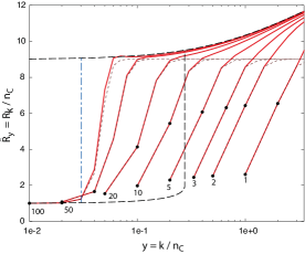
Fig. 2 compares the approximation (79) to the exact recursion (70) at finite $n_{C}$, and characterizes the convergence to the eikonal approximation at large $n_{C}$. When the small-$k$ asymptotic expansion is initialized with values ${\hat{R}}_{0}$ and ${\hat{R}}_{1}$ derived from Eq. (78), the exact recursion solutions remain close to that approximation over the interval between ${\bar{x}}_{1}$ and ${\bar{x}}_{3}$. The WKB solution has captured much of the finite-size scaling even though the effective potential is approximated with the large-deviations scaling limit. When $y$ is large enough that $\hat{R}$ exceeds the upper fixed-point value ${\bar{x}}_{3}$, the recursion solutions converge on the exact continuum value (73).

Figure 2: Finite-$n_{C}$ evaluations (solid) of the exact recursion relation (70), initiated at ${\hat{R}}_{0}$ and ${\hat{R}}_{1}$ (circles) using values from Eq. (79). That approximation (red-dashed) saturates at ${\bar{x}}_{3}/{\bar{x}}_{1}$. The lower and upper branches of the solution to the quadratic equation (72) are shown in black-dash (vertical connection is the upper limit where solutions exist on the lower branch). Equal-area value $y_{0}$ of Eq. (81), shown connecting the upper and lower branches $R\!\left(y\right)$ is approached by the recursion solutions at large $n_{C}$.

IV.2 Two-dimensional cross-catalytic CRN, and eikonal approximation at boundaries

To demonstrate the use of eikonals in a model with similar qualitative behavior that is not solvable in closed form, Fig. 3 shows a symmetric cross-catalytic CRN with the same fixed point structure along its axis of symmetry as the previous CRN. Recursion relations in this model were solved and compared to numerical simulations in Krishnamurthy:CRN_moments:17 ; Smith:CRN_moments:17 only along the axis of symmetry.

Figure 3: A network with two species labeled $A$ and $B$ in a cross-catalytic configuration. The fixed points for both $A$ and $B$ are the same as those for $A$ in the CRN of Fig. 1.

The reaction schema corresponding to Fig. 3 is

$$\varnothing \xrightleftharpoons[k_{2}]{\epsilon}{\rm A} {\rm A}+{\rm B} \xrightleftharpoons[{\bar{k}}_{1}]{k_{1}}2{\rm A}+{\rm B}$$

$$\varnothing \xrightleftharpoons[k_{2}]{\epsilon}{\rm B} {\rm B}+{\rm A} \xrightleftharpoons[{\bar{k}}_{1}]{k_{1}}2{\rm B}+{\rm A},$$ (82)

and its mean-field equation of motion (10) for numbers $n_{A}$ of species $A$ and $n_{B}$ of species $B$ is

$$\frac{dn_{A}}{d\tau} =\epsilon-k_{2}n_{A}+n_{B}\left(k_{1}n_{A}-{\bar{k}}_{1}n_{A}^{2}\right)$$

$$\frac{dn_{B}}{d\tau} =\epsilon-k_{2}n_{B}+n_{A}\left(k_{1}n_{B}-{\bar{k}}_{1}n_{B}^{2}\right).$$ (83)

Examples of the mean-field flow solutions, and more detailed properties of the escape eikonals, are provided in App. B, and we summarize only novel features here.

Figure 4: Skeleton of trajectories determining the topological domains of the CRN from Fig. 3. Solutions to the mean-field equations (83) from Fig. 11 in the appendix are shown in thin black. A converging separatrix (blue heavy) passing through the saddle separates the basins of attraction of the two fixed points. An escape separatrix (red heavy), the locus of points reached with equal probability from either fixed point, also passes through the saddle and is otherwise contained in the basin of attraction of the lower fixed point.

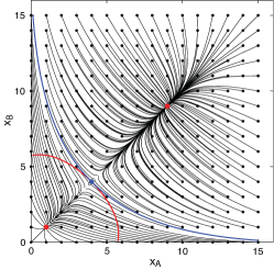
The topology of the space of trajectories is delimited by the skeleton shown in Fig. 4. An attracting separatrix divides the basins of attraction of the two stable fixed points. For this CRN (see App. B), escape eikonals never cross, so they form a foliation of the space of $n$ values. They are partitioned across the axis of symmetry by escape eikonals from the stable fixed points either to the saddle or to $x_{A}=x_{B}=0$ or $\infty$, along which the integral $\int\eta\,dx$ gives the relative depth of the minima of the effective potential $\hat{\Xi}\!\left(x\right)$. An escape separatrix, the locus of points with equal probability to be reached upon escape from either fixed point, emanates from the saddle, and is entirely contained within the basin of attraction of the lower fixed point.

Eikonal solutions along the non-asymptotic boundary

The $A\leftrightarrow B$ exchange symmetry of this model was used in Krishnamurthy:CRN_moments:17 ; Smith:CRN_moments:17 to reduce the recursion relations for moment ratios to a pair of self-consistent solutions similar in form to those for the 1-species autocatalytic CRN. The generator in the moment representation (32) is a 2-dimensional discrete Laplacian, given in Eq. (95). Its solutions off the diagonal depend on boundary conditions at $k_{A}=0$ or $k_{B}=0$ where the nonzero moment order need not lie in any asymptotic regime. In the limit $y_{B}\rightarrow 0$, an estimate for $y_{A}$ is given by

$$y_{A}=\frac{1}{{\hat{R}}_{B}}\left(\frac{{\kappa}_{2}{\hat{R}}_{A}-\varepsilon}{{\kappa}_{1}-{\bar{\kappa}}_{1}{\hat{R}}_{A}}\right)-{\hat{R}}_{A}$$ (84)

In Eq. (84) ${\hat{R}}_{B}\!\left(y_{A},0\right)$ is not given, but for $y\sim 1$ where the boundary is not very far from the diagonal, the approximation ${\hat{R}}_{B}\approx{\hat{R}}_{A}$ permits a closed-form comparison with Eq. (73) which applies to both $y_{A}$ and $y_{B}$ along the diagonal. An approximation of the effective potential by time-reversing trajectories, developed in App. B shows that the transfer of control between the two fixed points occurs along a roughly linear contour $y_{A}+y_{B}\approx 2y_{0}$ from Eq. (81).

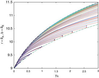
Fig. 5 illustrates the use of eikonals that emerge from neighborhoods of the diagonal to approximate the boundary conditions at $k_{B}=0$. It emphasizes that the boundary values at any point are governed not by propagation along the boundary, but by the values of moment ratios near the diagonal. Thus, in a population process with $P$ fluctuating species, although the boundary with undetermined conditions is a $\left(2P-1\right)$-dimensional hypersurface, the behavior along the boundary is controlled by neighborhoods of a discrete set of interior fixed points and the parameters of $\mathcal{L}$.

Figure 5: ${\hat{R}}_{A}\!\left(y_{A},y_{B}\right)$ (red-toned lines and symbols) and ${\hat{R}}_{B}\!\left(y_{A},y_{B}\right)$ (blue-toned lines and symbols) for eikonals emanating from neighborhoods of the escape trajectory between the lower fixed point and the saddle into the region $y_{B}<y_{A}$. Trajectories terminating in dots are truncated at the last point along the discrete numerical integral before the corresponding $y_{B}$ passes below zero. Upper black dashed curve is the eikonal solution (73) along the diagonal, and lower green dashed curve is the estimation (84). The asymmetry ${\hat{R}}_{B}-{\hat{R}}_{A}\geq 0$ remains small over the regions shown and increases with increasing $x_{A},x_{B}\lesssim{\bar{x}}_{3}$.

IV.3 Selkov model: asymmetric autocatalysis with breakdowns in the simple eikonal approximation

To present a case in which even the coarsest WKB approximation (78) cannot readily be obtained without continuum methods, Fig. 6 shows a CRN known as the Selkov model, which was treated with eikonal methods by Dykman et al. Dykman:chem_paths:94 . The Selkov model is an asymmetric autocatalytic system for which we can choose fixed points and residence times similar to those in the cross-catalytic CRN, though the eikonals in the two models show qualitative differences.

Figure 6: The Selkov model: an asymmetric autocatalytic CRN with two species $A$ and $B$. The model can yield fixed points with the same spacing and similar effective potential depths to the cross-catalytic network of Fig. 3, but on a line of negative rather than positive slope.

The reaction schema for Fig. 6 is

$$\varnothing \xrightleftharpoons[{\bar{k}}_{1}]{k_{1}}{\rm A} {\rm A}+2{\rm B} \xrightleftharpoons[{\bar{k}}_{2}]{k_{2}}3{\rm B} {\rm B} \xrightleftharpoons[{\bar{k}}_{3}]{k_{3}}\varnothing.$$ (85)

The fixed points of the Selkov model lie along a line

$$n_{\rm A}+n_{\rm B}=\frac{2\left(k_{1}+{\bar{k}}_{3}\right)}{\left({\bar{k}}_{1}+k_{3}\right)}-\frac{\left({\bar{k}}_{1}-k_{3}\right)}{\left({\bar{k}}_{1}+k_{3}\right)}\left(n_{\rm A}-n_{\rm B}\right),$$ (86)

Fig. 7 shows the solutions to the mean-field equations (10) for $\left({\bar{k}}_{1}-k_{3}\right)/\left({\bar{k}}_{1}+k_{3}\right)=-1/3$.

Figure 7: Flowfields from the mean-field equations (10) for the Selkov model. Parameters were chosen to place fixed points at $\left({\bar{x}}_{A},{\bar{x}}_{B}\right)=\left\{\left(2,80\right),\left(8,68\right),\left(18,48\right)\right\}$. Trajectories satisfy $d_{\tau}\left({{\rm n}}_{\rm A}+{{\rm n}}_{\rm B}\right)=0$ where they pass through the line (86) connecting the fixed points.

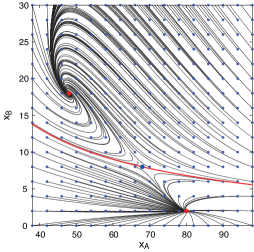
Fig. 8 shows the skeleton eikonals for the escape system of the Selkov model, reproducing features observed in Dykman:chem_paths:94 . Further detail is provided in App. C.

Figure 8: Skeleton for escape trajectories in the Selkov model. Eikonals from stable fixed points to the saddle are (heavy black). Trajectories originating counterclockwise from those double back and cross, creating a singular measure, in caustics (heavy red). The innermost limit of these rebounding trajectories is the limiting ray (thin black). Each point between the limiting ray and caustic is crossed by two trajectories, and each trajectory is crossed continuously before that point, requiring modification of the eikonal approximation.

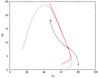
In contrast to the cross-catalytic CRN (82), in which every point $n$ is traversed by a unique escape trajectory and has a well-defined eikonal approximation to the escape probability, the Selkov model at parameters shown possesses two caustics emanating from the saddle point. Caustics are regions where the momentum-space WKB approximation breaks down as stationary trajectories from finite measure converge on a subsurface of measure zero. These caustics are formed as escapes diverging counterclockwise from the eikonal to the saddle turn back and cross. The innermost returning ray on each side of the saddle is the limiting ray, the boundary of the domain of validity of the simple stationary-path approximation.

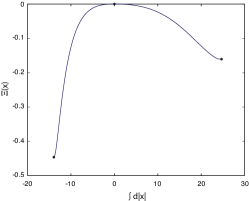
Finite-size effects may again be estimated by the coarse WKB approximation (78), but now the escape equations of motion must be solved to estimate the relative depths of the effective potential at the fixed point. Fig. 9 shows $\int\eta\,dn$ along the escape eikonals from the two stable fixed points to the saddle in Fig. 8. These give values $\hat{\Xi}\!\left({\bar{x}}_{1}\right)$ and $\hat{\Xi}\!\left({\bar{x}}_{3}\right)$ determining relative residence times and the first-passage time as a function of $n_{C}$.

Figure 9: $\int\eta\,dn$ along the eikonals from the two stable fixed points to the saddle gives the well depths of the effective potential. For these parameters $\hat{\Xi}\!\left({\bar{x}}_{1}\right)=-0.4462$ and $\hat{\Xi}\!\left({\bar{x}}_{3}\right)=-0.1606$. The difference, $0.2856$, is $\sim 4\times$ the difference for the 1-dimensional autocatalytic model shown in Fig. 7 of Smith:CRN_moments:17 , and about twice the difference of the cross-catalytic model shown in Fig. 14.

Using the convention for large-deviations scaling that $\bar{n}=n_{C}\bar{x}$ with fixed points

$${\bar{x}}_{1} =\left(80,2\right), {\bar{x}}_{3} =\left(48,18\right),$$ (87)

control of both moment ratios ${\hat{R}}_{A}$ and ${\hat{R}}_{B}$ is expected to switch between the fixed points along the line

$$\begin{array}[]{c}\left[\begin{array}[]{cc}y_{A}&y_{B}\end{array}\right]\\ \phantom{\mbox{}}\end{array}\left[\begin{array}[]{c}\log\left(48/80\right)\\ \log\left(18/2\right)\end{array}\right] =\hat{\Xi}\!\left({\bar{x}}_{3}\right)-\hat{\Xi}\!\left({\bar{x}}_{1}\right),$$ (93)

similar to the linear front $y_{A}+y_{B}=2y_{0}$ seen for the cross-catalytic CRN (82). Further details concerning trajectories and also the phenomenology of the conjugate variables $\eta$ is provided in App. C.

V Concluding remarks

We have considered the properties of a third representation of the generator of a stochastic CRN complementing its transition matrix and Liouville operator, expressed directly in the lattice of factorial moments of a probability distribution over number states. This generator provides a potentially efficient connection between nearby moments, but suffers the limitation that its boundary conditions are not simple to handle for high-dimensional systems.

We have shown how a continuum approximation, assuming slow variation of the ratios of adjacent factorial moments, combines with information already familiar from momentum-space WKB methods, to provide a leading exponential estimate for the values of moments throughout the lattice. The limit (49), in which the generator of the moment representation reduces to the Liouville operator on a stationary $\mathcal{L}=0$ solution, defines a map from the orders $k$ of factorial moments to positions along large-deviation trajectories that control the leading exponential behavior of moment ratios in neighborhoods of $k$.

Whereas for direct solution of the moment recursion equations, boundary conditions are difficult to specify where some components of $k$ become small, in the momentum-space WKB approximation solutions are propagated to the boundary along rays emanating from fixed points in the interior, as in the Freidlin-Wentzell approach to computing boundary values for solutions to diffusions on basins of attraction. Position-space WKB methods can be used to approximate finite-size corrections using the simplified scale factors and rate functions computed from the large-deviations limit.

The moment representation also provides a natural interpretation for the coherent-state fields $\left({\xi}^{\dagger},\xi\right)$ which appear in Hamilton-Jacobi theory as a canonical transform of the number-potential fields $\left(\eta,n\right)$ that are the natural variables for momentum-space WKB methods. Whereas $n$ is the index, and $\eta$ the log-derivative, of the stationary distribution, $\xi$ takes a value equal to the ratio $R$ of adjacent factorial moments. $e^{\eta}={\xi}^{\dagger}$ is then the ratio of probability flow rates normal to isoclines of the stationary probability.

The three representations of the generator of a stochastic CRN use the three classes of random variables as bases: ${\sigma}_{{\rm n}}$ (the discrete indicator function on states, for the distribution ${\rho}_{{\rm n}}$), ${{\rm n}}^{\underline{k}}$ (discrete powers, for moments ${\Phi}_{k}$), and $z^{{\rm n}}$ (continuous tilts, for the MGF $\phi\!\left(z\right)$). The well-known direct interconversions Doi:SecQuant:76 ; Doi:RDQFT:76 ; Peliti:PIBD:85 ; Peliti:AAZero:86 and the new one derived in Krishnamurthy:CRN_moments:17 ; Smith:CRN_moments:17 facilitate choosing bases with good convergence properties for different classes of observables of interest. The connection among the three through the large-deviations limit derived here, in addition to providing approximation methods, shows connections of meaning across the representations that are sometimes not apparent in their more indirect, detailed interconversions.

Acknowledgments

DES was supported in part by NASA Astrobiology CAN-7 award NNA17BB05A through the College of Science, Georgia Institute of Technology, and by the Japanese Ministry of Education, Culture, Sports, Science, and Technology (MEXT) through the World Premiere International program. He also thanks the Physics Department at Stockholm University for hospitality in May $2016-2019$, when some of this work was carried out.

Appendix A Matched asymptotic expansions of the exact recursion for the one-species autocatalytic CRN

For a one-dimensional system, sufficient boundary data is present in the Liouville operator $\mathcal{L}$ that formally the exact recursion (32) at steady state is sufficient to fix a solution. However, the asymptotic nature of the recursion makes its application a problem of stabilization in most cases, with low-order moments of interest being sensitive to arithmetic precision or truncation errors in the series. There is thus a practical use for the WKB approximation (78) in the estimation of finite-size effects, which we describe here in relation to the exact recursion and to the large-system limit.

We use as an example an instance of the one-species CRN (68) drawn from Krishnamurthy:CRN_moments:17 ; Smith:CRN_moments:17 , with parameters ${\bar{k}}_{1}=1$, $k_{1}=14$, $\epsilon=36$, $k_{2}=49$. At these parameters the mean-field rate equation (69) has stable zeros at $n/n_{C}={\bar{x}}_{1}=1$ and ${\bar{x}}_{3}=9$, and a saddle-point zero ${\bar{x}}_{2}=4$.

Traditionally, moment series are solved recursively upward in $k$: ${\Phi}_{0}\equiv 1$ by normalization of probability, $R_{0}\equiv{\Phi}_{1}$ is estimated by the mean-field equations, and so forth. The lower-order moments are assumed to be not only the larger components of the variation, but also those components most robust in a simple model against parameter imprecision or mis-specification of model details Smith:evo_games:15 . Therefore, as emphasized in Krishnamurthy:CRN_moments:17 ; Smith:CRN_moments:17 , it is counterintuitive that the recursive solution for ${\hat{R}}_{k}$ is anchored not at $k\rightarrow 0$ by $x$ in the mean-field solution, but rather at $k\rightarrow\infty$ by ratios of parameters in $\mathcal{L}$ that generally differ from the mean of $x$ at any of its fixed points, and which are related to probability currents that can arise in networks of nonzero deficiency (see Feinberg:def_01:87 ; Anderson:product_dist:10 for elaborations on deficiency). The downward-going recursion is stable for $k/\left<{\rm n}\right>$ sufficiently large, so the asymptotic value can be imposed on $R_{k}$ at large finite $k$, and truncation errors are exponentially attenuated as $k$ decreases. However, the downward recursion becomes unstable below some characteristic scale for $k/\left<{\rm n}\right>$, and errors that were initially attenuated are amplified, along with numerical precision errors, in a diverging asymptotic expansion that cannot be continued if $n_{C}$ is large enough.

Therefore an upward-going asymptotic expansion must be initiated from an ansatz at small $k$, and matched to the downgoing expansion at an intermediate scale where both are marginally stable. Because the upward-going solution is stable in increasing $k$, imprecision in the ansatz is attenuated, but this also means that the matching conditions to the downgoing asymptotic solution provide weak constraints on the small-$k$ ansatz at large $n_{C}$. It is to substitute for this weak constraint that the WKB approximation (78) can be useful.

Fig. 10 shows how the WKB starting conditions for low-order modes relates to full solutions where those exist, and to Gillespie simulations for one case (at $n_{C}=1$). The figure shows solutions to the exact recursion equation (70) for values $n_{C}=\left\{1,2,3,5,10,20,50,100\right\}$. For the first three of these values, the recursion is stable all the way to $k=1$, and at $n_{C}=1$ the low-order modes that can be estimated from simulation are excellent matches for the recursive solution. Upward-going solutions, initiated with $R_{0}$ and $R_{1}$ from the WKB approximation are shown for all eight values of $n_{C}$, and compared to the downward-going solutions for $n_{C}=\left\{1,2,3\right\}$.

Figure 10: A set of solutions at $n_{C}=\left\{1,2,3,5,10,20,50,100\right\}$ to the exact recursion relations for the one-species autocatalytic CRN (68). First panel illustrates application of the matched asymptotic expansions explained in Krishnamurthy:CRN_moments:17 ; Smith:CRN_moments:17 in the transition region $y\gtrsim 14$ for this model. Second panel expands the abscissa to characterize the WKB approximation (79). For $n_{C}=\left\{1,2,3\right\}$ the upper asymptotic boundary condition extends stably to $k=1$, and agrees closely with the $\hat{R}$ values from Gillespie simulations (black asterisks) for $n_{C}=1$. Upward-going solutions initiated at values ${\hat{R}}_{0}$ (colored dots) from the WKB approximation are computed at all $n_{C}$; their deviation from the downward solutions gives an estimate of the error from the WKB approximation at small $n_{C}$. Horizontal dashed green line is the upper asymptotic value ${\hat{R}}\leq 14$ for these parameters; that value is also the characteristic scale for matching of asymptotic expansions (vertical green dashed line). Black-dashed upper curve is the higher branch $\hat{R}\!\left(y\right)$ from Eq. (72).

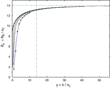
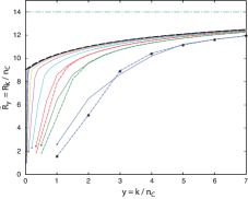
The figure shows that the difference between the WKB ansatz and the exact solution is smaller than the separation between adjacent values of $n_{C}$, and decreases as $n_{C}$ grows. Within each pair of curves (solid, dashed), attenuation of the error in the WKB initial condition with increasing $k$ is shown by the rapid convergence of the upgoing and exact downgoing solutions. The figure shows also that for $n_{C}\sim 100$ the solution is well-approximated by the eikonal solution. The upward-going recursive solutions only are shown, on logarithmic scale to expand the transition region between branches of Eq. (72), in Fig. 2 in the text.

Appendix B Generator, trajectories, and effective potential for the two-species cross-catalytic CRN

The cross-catalytic CRN (82) exactly recapitulates the large-deviation properties of the autocatalytic CRN (68) along the axis of symmetry $x_{A}=x_{B}$, and approximates the solutions to the exact recursions, though in more complicated form, at finite $n_{C}$, as derived in Smith:CRN_moments:17 . Its large-deviation behavior remains simple in the sense that escape trajectories do not cross (so the eikonal approximation is valid everywhere), and that they converge strongly toward time-reverses of solutions to the mean-field equations of motion (10) in neighborhoods of the diagonal, leading to a computationally efficient approximation of the effective potential $\hat{\Xi}\!\left(x\right)$ in that region. Away from the diagonal, however, the irreversible nature of the CRN becomes visible as escape trajectories deviate from mean-field trajectories, leading to most-probable excursions that are loops, and a non-trivial relation between the separatrices for mean-field flow and for escapes. Here we provide details of these properties of the eikonal approximation, retaining the same parameters $\epsilon=36$, $k_{2}=49$, $k_{1}=14$, ${\bar{k}}_{1}=1$ used for the 1-species CRN from App. A.

We begin by noting the exact form of the 2-species generator in the moment representation. A set of descaled variables was introduced in Smith:CRN_moments:17

$${\omega}_{+} \equiv\epsilon/k_{1} {\omega}_{\Delta} \equiv k_{2}/{\bar{k}}_{1}-{\omega}_{+}$$

$$=\varepsilon n_{C}^{2}/{\kappa}_{1} =k_{2}n_{C}^{2}/{\bar{\kappa}}_{1}-{\omega}_{+}$$

$$\equiv{\hat{\omega}}_{+}n_{C}^{2} ={\hat{\omega}}_{\Delta}n_{C}^{2}$$ (94)

The form of the exact generator in the moment hierarchy is

$$-\frac{{\left(\Lambda\Phi\right)}_{k}}{{\bar{k}}_{1}}=-{\omega}_{\Delta}\left(k_{A}+k_{B}\right){\Phi}_{k}+{\omega}_{+}\left[k_{A}\left(K_{1}{\Phi}_{k-1_{a}}-{\Phi}_{k}\right)+k_{B}\left(K_{1}{\Phi}_{k-1_{b}}-{\Phi}_{k}\right)\right]$$

$$\quad\mbox{}+K_{1}^{2}\left[k_{A}\left(\frac{{\Phi}_{k+1_{b}}}{K_{1}}-\frac{{\Phi}_{k+1_{a}+1_{b}}}{K_{1}^{2}}\right)+k_{B}\left(\frac{{\Phi}_{k+1_{a}}}{K_{1}}-\frac{{\Phi}_{k+1_{a}+1_{b}}}{K_{1}^{2}}\right)\right]$$

$$\quad\mbox{}+K_{1}\left[k_{A}\left(k_{A}-1\right)\left({\Phi}_{k-1_{a}+1_{b}}-\frac{{\Phi}_{k+1_{b}}}{K_{1}}\right)+k_{A}k_{B}\left(2{\Phi}_{k}-\frac{{\Phi}_{k+1_{a}}}{K_{1}}-\frac{{\Phi}_{k+1_{b}}}{K_{1}}\right)+k_{B}\left(k_{B}-1\right)\left({\Phi}_{k+1_{a}-1_{b}}-\frac{{\Phi}_{k+1_{a}}}{K_{1}}\right)\right]$$

$$\quad\mbox{}+k_{A}k_{B}\left[\left(k_{A}-1\right)\left(K_{1}{\Phi}_{k-1_{a}}-{\Phi}_{k}\right)+\left(k_{B}-1\right)\left(K_{1}{\Phi}_{k-1_{b}}-{\Phi}_{k}\right)\right].$$ (95)

Substituting the exact moment ratios $R_{Ak}$ and $R_{Bk}$ for shifts in the moment index, Eq. (95) becomes

$$-\frac{{\left(\Lambda\Phi\right)}_{k}}{{\bar{k}}_{1}}=\left\{-{\omega}_{\Delta}\left(k_{A}+k_{B}\right)+{\omega}_{+}\left[k_{A}\left(\frac{K_{1}}{R_{Ak}}-1\right)+k_{B}\left(\frac{K_{1}}{R_{Bk}}-1\right)\right]\right.$$

$$\quad\mbox{}+\left.K_{1}^{2}\left[k_{A}\frac{R_{B,k+1_{b}}}{K_{1}}\left(1-\frac{R_{A,k+1_{a}+1_{b}}}{K_{1}}\right)+k_{B}\frac{R_{A,k+1_{a}}}{K_{1}}\left(1-\frac{R_{B,k+1_{a}+1_{b}}}{K_{1}}\right)\right]\right.$$

$$\quad\mbox{}+\left.K_{1}\left[k_{A}\left(k_{A}-1\right)\frac{R_{B,k+1_{b}}}{K_{1}}\left(\frac{K_{1}}{R_{A,k+1_{b}}}-1\right)+k_{A}k_{B}\left(2-\frac{R_{A,k+1_{a}}}{K_{1}}-\frac{R_{B,k+1_{b}}}{K_{1}}\right)+k_{B}\left(k_{B}-1\right)\frac{R_{A,k+1_{a}}}{K_{1}}\left(\frac{K_{1}}{R_{B,k+1_{a}}}-1\right)\right]\right.$$

$$\quad\mbox{}+\left.k_{A}k_{B}\left[\left(k_{A}-1\right)\left(\frac{K_{1}}{R_{Ak}}-1\right)+\left(k_{B}-1\right)\left(\frac{K_{1}}{R_{Bk}}-1\right)\right]\right\}{\Phi}_{k}.$$ (96)

In the large-system substitution of moment ratios (33), the exact expression (96) reduces to

$$-\frac{{\left(\Lambda\Phi\right)}_{k}}{{\bar{\kappa}}_{1}n_{C}} \rightarrow\left\{-{\hat{\omega}}_{\Delta}\left(y_{A}+y_{B}\right)+\left[{\hat{\omega}}_{+}+\left(y_{A}+{\hat{R}}_{Ay}\right)\left(y_{B}+{\hat{R}}_{By}\right)\right]\left[y_{A}\left(\frac{{\hat{K}}_{1}}{{\hat{R}}_{Ay}}-1\right)+y_{B}\left(\frac{{\hat{K}}_{1}}{{\hat{R}}_{By}}-1\right)\right]\right\}{\Phi}_{k},$$ (97)

where ${\kappa}_{1}/{\bar{\kappa}}_{1}\equiv{\hat{K}}_{1}=K_{1}/n_{C}$.

The Liouville operator for the CRN (82) in number-potential fields is computed by standard methods Smith:CRN_moments:17 to be

$$\hat{\mathcal{L}} =\left(1-e^{{\eta}_{A}}\right)\left(\epsilon+{\kappa}_{1}x_{A}x_{B}\right)+\left(1-e^{-{\eta}_{A}}\right)\left({\kappa}_{2}+{\bar{\kappa}}_{1}x_{A}x_{B}\right)x_{A}$$

$$\mbox{}+\left(1-e^{{\eta}_{B}}\right)\left(\varepsilon+{\kappa}_{1}x_{A}x_{B}\right)+\left(1-e^{-{\eta}_{B}}\right)\left({\kappa}_{2}+{\bar{\kappa}}_{1}x_{A}x_{B}\right)x_{B}$$ (98)

Under the mapping (62), equations (97) and (98) are proportional in the same manner as Eq. (75) showed for the 1-species model.

The general-form eikonal equations that follow from $\hat{\mathcal{L}}$ in Eq. (98) are

$$d_{\tau}n_{A} =e^{{\eta}_{A}}\left(\epsilon+k_{1}x_{A}x_{B}\right)-e^{-{\eta}_{A}}\left(k_{2}+{\bar{k}}_{1}x_{A}x_{B}\right)x_{A}$$

$$d_{\tau}n_{B} =e^{{\eta}_{B}}\left(\epsilon+k_{1}x_{A}x_{B}\right)-e^{-{\eta}_{B}}\left(k_{2}+{\bar{k}}_{1}x_{A}x_{B}\right)x_{B}$$

$$d_{\tau}{\eta}_{A} =\left(2-e^{{\eta}_{A}}-e^{{\eta}_{B}}\right)k_{1}x_{B}+\left(1-e^{-{\eta}_{A}}\right)\left(k_{2}+2{\bar{k}}_{1}x_{A}x_{B}\right)$$

$$\mbox{}+\left(1-e^{-{\eta}_{B}}\right){\bar{k}}_{1}x_{B}^{2}$$

$$d_{\tau}{\eta}_{B} =\left(2-e^{{\eta}_{A}}-e^{{\eta}_{B}}\right)k_{1}x_{A}+\left(1-e^{-{\eta}_{A}}\right){\bar{k}}_{1}x_{A}^{2}$$

$$\mbox{}+\left(1-e^{-{\eta}_{B}}\right)\left(k_{2}+2{\bar{k}}_{1}x_{A}x_{B}\right)$$ (99)

Fig. 11 shows the solutions to these equations at $\eta\equiv 0$, which are the mean-field solutions (10). The two basins of attraction are divided by a separatrix, shown as the blue curve in Fig. 4 in the text.

Figure 11: Stationary trajectories at ${\eta}_{A}={\eta}_{B}=0$ are solutions to the mean-field equations (83). Dots indicate starting points of trajectories in this numerical integral. Curvature toward the axis of symmetry $x_{A}=x_{B}$ indicates that this axis is a curve of slowest departure from the saddle fixed point $\left(4,4\right)$, and slowest approach to the attracting fixed points $\left(1,1\right)$ and $\left(9,9\right)$.

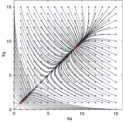
Fig. 12 shows corresponding escape trajectories at $\eta\neq 0$, originating in very close neighborhoods of the stable fixed points. It can be seen that escapes originating close to the diagonal, as they approach the saddle, diverge and that escapes from the two fixed points run parallel. Their line of convergence is the escape separatrix shown in dashed red in Fig. 12 and also in Fig. 4. It is clear that the escape separatrix is the locus of points with equal probability to be reached from either fixed point Dykman:chem_paths:94 , because the probabilities on this curve are conditional upon reaching the saddle, for which the probability is the same from either fixed point by the construction (53) of the effective potential. Because the conjugate momentum field $\eta$ is continuous across this curve, $-\int\eta\,dn$ converges to the log-probability along the separatrix from either side.

Figure 12: A representative sample of escape rays from the three fixed points. For the symmetric model, escape rays converge to the time-reverses of solutions to the classical equations of motion (10) in infinitesimal neighborhoods of the fixed points (and along the eikonals from the stable fixed points to the saddle. The escape separatrix falls where rays from the lower and upper fixed points become parallel.

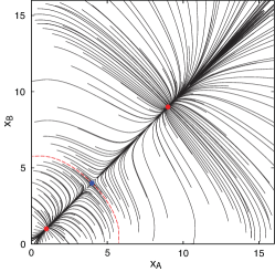
Comparison of Fig. 11 and Fig. 12 shows that escape trajectories converge to time-reverses of mean-field trajectories in neighborhoods of the diagonal – a property that is exact for 1-dimensional systems, noted in the deerivation of Eq. (77) fn. 5 – and that they are exact reverses along the diagonal, explaining why the cross-catalytic CRN recovers the large-deviations limit of the autocatalytic CRN on the axis of symmetry.

However, away from the diagonal escape trajectories are concave toward the origin, whereas converging trajectories are concave away from the origin, reflecting the intrinsic irreversibility of the CRN rules. Two consequences are that excursions from a basin, which relax by mean-field return, are loops, and also that the escape separatrix is entirely contained within the basin of attraction of the lower fixed point ${\bar{x}}_{1}$. While off-diagonal excursions are subleading relative to escapes along the diagonal, and thus do not alter the balance of probability flows in the large-deviations limit, it follows that there is a net flow of probability from the fixed point ${\bar{x}}_{3}$ to the fixed point ${\bar{x}}_{1}$ by such excursions.

Time-reversal approximation to the effective potential

The eikonal approximation to the full effective potential surface can be tedious to extract. The existence of a Liouville theorem for the dynamical system with “Hamiltonian” $\mathcal{L}$ implies that trajectory integrals have equal numbers of stable and unstable directions integrated either forward or backward in time, and these amplify errors in boundary conditions and arithmetical precision limits exponentially into macroscopic errors.

The assimilation of escapes to time-reverses of converging trajectories near fixed points, and in the cross-catalytic CRN along the whole skeleton of eikonals between fixed and saddle points, leads to an approximation in which $\eta$ is chosen to place $\mathcal{L}=0$ and to exactly reverse velocity at each point $x$. Effectively, one treats probability-current balance along eikonals in higher dimensions as if it were exact, as it is in one dimension, ignoring refractive effects on the stationary trajectory. The resulting $\eta$ field does not satisfy the true eikonal equation for escapes, but for this CRN the corrections will become small near the diagonal that determines the main scales of the effective potential.

The time-reversing $\eta$ values in the cross-catalytic CRN, corresponding to the exact solution in the one-variable CRN, are

$${\bar{\eta}}_{A} \approx\log\left[\frac{\left({\kappa}_{2}+{\bar{\kappa}}_{1}{\bar{x}}_{A}{\bar{x}}_{B}\right){\bar{x}}_{A}}{\left(\varepsilon+{\kappa}_{1}{\bar{x}}_{A}{\bar{x}}_{B}\right)}\right]=\log{\bar{x}}_{A}-\log{\hat{R}}_{A}$$

$${\bar{\eta}}_{B} \approx\log\left[\frac{\left({\kappa}_{2}+{\bar{\kappa}}_{1}{\bar{x}}_{A}{\bar{x}}_{B}\right){\bar{x}}_{B}}{\left(\varepsilon+{\kappa}_{1}{\bar{x}}_{A}{\bar{x}}_{B}\right)}\right]=\log{\bar{x}}_{B}-\log{\hat{R}}_{B}.$$ (100)

The resulting expressions for the moment ratios, corresponding to Eq. (76) for the 1-species model, are

$${\hat{R}}_{A}={\bar{x}}_{A}e^{-{\bar{\eta}}_{A}} \approx\frac{\left(\varepsilon+{\kappa}_{1}{\bar{x}}_{A}{\bar{x}}_{B}\right)}{\left({\kappa}_{2}+{\bar{\kappa}}_{1}{\bar{x}}_{A}{\bar{x}}_{B}\right)}$$

$$={\bar{x}}_{B}e^{-{\bar{\eta}}_{B}} ={\hat{R}}_{B}.$$ (101)

Note that in this approximation ${\hat{R}}_{A}$ and ${\hat{R}}_{B}$ are the same, motivating the equivalence used to solve Eq. (84). The stationary-point relation between $y$, $x$, and $\hat{R}$ from Eq. (62) remains

$$y_{A,B}={\bar{x}}_{A,B}-{\hat{R}}_{A,B}\!\left(\bar{x}\right).$$ (102)

Fig. 13 shows the two positive branches of the solution $\hat{R}\!\left(y\right)$ to conditions (100,102), coinciding with the solutions (73) of the autocatalytic CRN along the diagonal. These $\hat{R}$ values are well-approximated as functions of $y_{A}+y_{B}$ over most of the space.

Figure 13: The two branches of the solution $\hat{R}\!\left(y\right)$ in the time-reverse approximation (100) for $\bar{\eta}$. The branch controlled by the fixed point ${\bar{x}}_{1}$ is shaded blue, and the branch controlled by ${\bar{x}}_{3}$ is shaded red. Inset shows rotated axes to project the surface onto the coordinate $y_{A}+y_{B}$, showing that $\hat{R}\!\left(y\right)$ is almost independent of $y_{A}-y_{B}$.

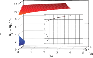
The time-reversing $\eta$ values (100) give an approximation of the one-argument effective potential (54)

$$\hat{\Xi}\!\left(\bar{x}\right) \approx\int\sum_{p=a,b}{\bar{\eta}}_{p}d{\bar{x}}_{p}$$

$$=\sum_{p=a,b}{\bar{x}}_{p}\left[\log{\bar{x}}_{p}-1\right]-\int\log\hat{R}\!\left(\bar{x}\right)\,d\left({\bar{x}}_{A}+{\bar{x}}_{B}\right).$$ (103)

The corresponding result for the two-argument effective potential (58) tilted by $y=\bar{x}-\hat{R}$ becomes

$$\mathbf{\hat{\Xi}}\!\left(\bar{x};y\right) =\hat{\Xi}\!\left(\bar{x}\right)+\sum_{p=a,b}\left\{{\hat{R}}_{p}\left[\log{\hat{R}}_{p}-1\right]-{\bar{x}}_{p}\left[\log{\bar{x}}_{p}-1\right]\right\}$$

$$=\sum_{p=a,b}{\hat{R}}_{p}\left[\log{\hat{R}}_{p}-1\right]-\int\log\hat{R}\!\left(\bar{x}\right)\,d\left({\bar{x}}_{A}+{\bar{x}}_{B}\right).$$ (104)

In these two equations, ${\bar{x}}_{p}\left[\log{\bar{x}}_{p}-1\right]$ or ${\hat{R}}_{p}\left[\log{\hat{R}}_{p}-1\right]$ are local potential terms that can be computed without computing escape trajectories. The other term ($\int\log\hat{R}\!\left(\bar{x}\right)\,d\left({\bar{x}}_{A}+{\bar{x}}_{B}\right)$) still depends on a trajectory $\bar{x}$ terminating in the argument of $\Xi$. However, because in this approximation ${\hat{R}}_{A}\approx{\hat{R}}_{B}$, only the component $d\left({\bar{x}}_{A}+{\bar{x}}_{B}\right)$ contributes, and for small $x$, corrections from the dependence of ${\hat{R}}$ on $\left({\bar{x}}_{A}+{\bar{x}}_{B}\right)$ remain small.

Fig. 14 shows the approximate solution (103). The black line along the diagonal equals twice the value from the exact eikonal solution for the autocatalytic CRN (the cross-catalytic system scales as two duplicate copies of the autocatalytic system).

Figure 14: The effective potential $\hat{\Xi}\!\left(\bar{x}\right)$ from Eq. 103. The contour along the diagonal ${\bar{x}}_{A}={\bar{x}}_{B}$, equals $2\times\mbox{}$ the value of the one-species model from Smith:CRN_moments:17 . Colormap of the potential is projected onto the floor of the plot.

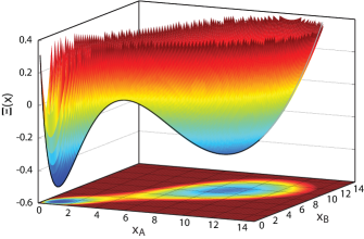
Appendix C Structure of escapes and estimation of the effective potential for the Selkov model

The Selkov model was analyzed by Dykman et al. Dykman:chem_paths:94 using eikonal methods, and the case we consider here was chosen to reproduce the major qualitative features seen in that analysis. Like the cross-catalytic CRN, the Selkov CRN has a cubic mean-field equation and one linear steady-state condition ensuring that all fixed points will lie along a line. It generalizes the cross-catalytic CRN, in which the fixed-point line is by construction the axis of symmetry under $A\leftrightarrow B$, to a 1-parameter degree of freedom setting the slope of the line. Unlike the cross-catalytic CRN, where the slope is 1, in the Selkov model the slope is negative. Thus the monotonicity of fixed-point values in $\left({\bar{x}}_{A},{\bar{x}}_{B}\right)$ is opposite for species $A$ and $B$, leading to a trade-off in the orders $k_{A}$ and $k_{B}$ along the front where control of fluctuations switches from the more-stable to the less-stable fixed point.

The asymmetric catalytic schema (85) that gives the Selkov model a negative slope for its fixed points also leads to vorticity in the stationary trajectories, which has the same sign for both classical mean-field equations and escape trajectories. Thus excursions that return to a fixed point are even more exaggerated loops in the Selkov model than in the cross-catalytic CRN. Escape trajectories also form caustics, leading to regions in the state space for which the eikonal approximation becomes invalid, a phenomenon noted for eikonals in first-passage problems by Maier and Stein Maier:caustics:93 and remarked in this model in Dykman:chem_paths:94 .

The parameters for the numerical example were chosen as follows: The free parameter determining the slope in the reaction schema (85) we denote as $\left({\bar{k}}_{1}-k_{3}\right)/\left({\bar{k}}_{1}+k_{3}\right)=\alpha$. The vorticity in the mean-field equations (10) increases as $\alpha$ decreases; to study its effect on escapes and caustics we set $\alpha=-1/3$ in the example.

By choice of the relative normalizations of ${{\rm n}}_{A}$ and ${{\rm n}}_{B}$ we may set $k_{2}={\bar{k}}_{2}$. By choice of the absolute normalization of ${\rm n}$ relative to the buffering species implicit in the Feinberg null species $\varnothing$, we may set ${\bar{k}}_{1}=1+\alpha=2/3$, $k_{3}=1-\alpha=4/3$.

To preserve as much similarity as possible to the previous two examples in which the fixed point numbers ${\bar{x}}_{1}:{\bar{x}}_{2}:{\bar{x}}_{3}$ were in the ratio $1:4:9$, we seek fixed points with the ratios $\left({\bar{x}}_{3}-{\bar{x}}_{2}\right):\left({\bar{x}}_{2}-{\bar{x}}_{1}\right)=5:3$. The smallest integer-valued fixed points with this property are given by assignments: $k_{2}=\left(1-{\alpha}^{2}\right)/\left(2\times{14}^{2}\right)\approx 0.0023$, ${\bar{k}}_{3}=2\left(1-\alpha\right)\times\left(36/49\right)\approx 1.9592$, $k_{1}=4\times 14-{\bar{k}}_{3}\approx 54.041$. The resulting three solutions for the fixed points are $\left({\bar{x}}_{A},{\bar{x}}_{B}\right)\in\left\{\left(80,2\right),\left(68,8\right),\left(48,18\right)\right\}$.

Solutions to the mean-field equations at these parameters are shown in Fig. 7, and those can be compared to solutions for escape trajectories in Fig. 15. In the second figure, we show only rays exiting counterclockwise to the eikonals from the fixed points that reach the saddle, to highlight the formation of caustics by rays that double back before reaching the saddle. The skeleton of boundary rays from this figure is plotted alone in Fig. 8 in the text.

Figure 15: Sets of escape rays from either stable fixed point (thin stroke), bounded on one side by the eikonal from the fixed point to the saddle (heavy black), and on the other by a caustic (heavy red). Rays departing from the eikonal very near the saddle converge toward limiting rays (heavy black).

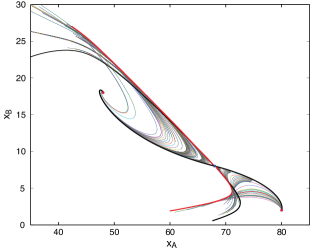
Integration of $\int\eta\,dn$ along the eikonals from the stable fixed points to the saddle gives the cut through the effective potential $\hat{\Xi}\!\left(x\right)$ along its minimizing contour shown in Fig. 9. The profile is qualitatively similar to that shown in Fig. 14 for the cross-catalytic CRN that these Selkov-model parameters were chosen to resemble. From the relative minima of $\hat{\Xi}\!\left(x\right)$ we may evaluate the WKB approximation (79) for the domains where the deeper fixed point ${\bar{x}}_{1}=\left(80,2\right)$ and the shallower fixed point ${\bar{x}}_{3}=\left(48,18\right)$ control moment ratios. The separatrix between these two is estimated to lie along the linear front

$$\begin{array}[]{c}\left[\begin{array}[]{cc}k_{A}&k_{B}\end{array}\right]\\ \phantom{\mbox{}}\end{array}\left[\begin{array}[]{c}\log\left(48/80\right)\\ \log\left(18/2\right)\end{array}\right] =n_{C}\left(\hat{\Xi}\!\left({\bar{x}}_{3}\right)-\hat{\Xi}\!\left({\bar{x}}_{1}\right)\right)$$ (110)

$$\approx\begin{array}[]{c}\left[\begin{array}[]{cc}k_{A}&k_{B}\end{array}\right]\\ \phantom{\mbox{}}\end{array}\left[\begin{array}[]{c}\log\left(3/5\right)\\ 2\log\left(3\right)\end{array}\right] \approx n_{C}\left(0.4462-0.1606\right).$$ (116)

Fig. 16 shows the behavior of the potential field $\eta$ along the two eikonals from the fixed points to the saddle and along neighboring escape trajectories. Consistent with the linear front (116) across which the dominant contribution to moments is expected to switch from the deeper to the shallower fixed point, $\eta$ is bounded by roughly linear horizons along rays escaping from the lower and upper fixed points, corresponding respectively to the maxima and minima of the cubic solution (76) in the one-dimensional model. The upper horizon for $\eta$ from the fixed point $\left(80,2\right)$, with normal $\approx\left[\;-1\;1\;\right]$ corresponds to the maximum of $\eta$ along the lower branch solution shown in the inset to Fig. 13 for the cross-catalytic model.

Figure 16: Field values $\eta$ along escape contours from the deeper fixed point $\left(80,2\right)$ in the potential of Fig. 9 (red) and the shallower fixed point $\left(48,18\right)$ (blue). $\eta$ values along eikonals from the stable fixed points to the saddle are heavy lines. $\eta$ integrated along escape contours reaches a maximum in the component $\sim\left[\;-1\;1\;\right]$, along all rays in a neighborhood of the eikonal. Hence $\int dn\eta$ giving the effective potential attains its maximum roughly along this horizon, in contrast to the maximum for the cross-catalytic CRN shown in Fig. 13 (inset), which occurs on a front of roughly constant $y_{A}+y_{B}$.

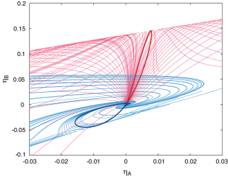
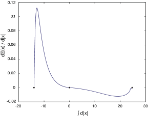
Fig. 16 shows also that $\eta\rightarrow 0$ on the approach to either stable or saddle fixed points, making a smooth continuation with the $\mathcal{L}\equiv 0$ condition satisfied along all mean-field trajectories. Thus, even though the curvature of $\hat{\Xi}\!\left(x\right)$ in the neighborhood of the deeper fixed point is not readily visible in Fig. 9 as it is for the cross-catalytic model in Fig. 14, the potential is quadratic in neighborhoods of all of its fixed points. Fig. 17 shows the gradient $d\Xi/d\left|n\right|$ (defined as $\eta\,dn/dn^{2}$ for the line element along the contour) equivalent to Eq. (80) along the tangent to the eikonals connecting the stable fixed points to the saddle. The gradient remains monotonic in neighborhoods of either fixed point, but its derivative is not monotone near the fixed point $\left(48,18\right)$, as a result of the vorticity and shear of all stationary trajectories in this region.

Figure 17: $d\Xi/d\left|n\right|$ versus distance $\int d\left|n\right|$ along the eikonals from the two fixed points to the saddle, giving the component of $\eta$ along the least improbable escape path. $\eta$ approaches zero linearly near the lower fixed point $\left(80,2\right)$, but its behavior is more complex near the upper fixed point $\left(48,18\right)$, due to the spiral exit of the escape ray shown in Fig. 8. The maximum value along the escape from the fixed point $\left(80,2\right)$ is similar to that for the cross-catalytic model, and comparable to the maximum on the horizon in Fig. 16.

References

- (1) Supriya Krishnamurthy and Eric Smith. Solving moment hierarchies for chemical reaction networks. J. Phys. A: Math. Theor., 50:425002, 2017.
- (2) Eric Smith and Supriya Krishnamurthy. Flows, scaling, and the control of moment hierarchies for stochastic chemical reaction networks. Phys. Rev. E, 96:062102, 2017.
- (3) N. G. van Kampen. Stochastic Processes in Physics and Chemistry. Elsevier, Amsterdam, third edition, 2007.
- (4) Martin Feinberg. Chemical reaction network structure and the stability of complex isothermal reactors – I. The deficiency zero and deficiency one theorems. Chem. Enc. Sci., 42:2229–2268, 1987.
- (5) David F. Anderson, George Craciun, and Thomas G. Kurtz. Product-form stationary distributions for deficiency zero chemical reaction networks. Bull. Math. Bio., 72:1947–1970, 2010.
- (6) Jeremy Gunawardena. Chemical reaction network theory for in-silico biologists. lecture notes, June 2003. vcp.med.harvard.edu/papers/crnt.pdf.
- (7) John C. Baez and Brendan Fong. Quantum techniques for studying equilibrium in reaction networks. J. Compl. Netw., 3:22–34, 2014. https://academic.oup.com/comnet/article-abstract/3/1/22/490572/Quantum-techniques-for-studying-equilibrium-in?redirectedFrom=fulltext.
- (8) Matteo Polettini and Massimiliano Esposito. Irreversible thermodynamics of open chemical networks. I. Emergent cycles and broken conservation laws. J. Chem. Phys., 141:024117, 2014.
- (9) M. Polettini, A. Wachtel, and M. Esposito. Dissipation in noisy chemical networks: the role of deficiency. arxiv:1507.00058v3, 2015.
- (10) Hugo Touchette. The large deviation approach to statistical mechanics. Phys. Rep., 478:1–69, 2009. arxiv:0804.0327.
- (11) M. I. Freidlin and A. D. Wentzell. Random Perturbations in Dynamical Systems. Springer, New York, second edition, 1998.
- (12) M. Doi. Second quantization representation for classical many-particle system. J. Phys. A, 9:1465–1478, 1976.
- (13) M. Doi. Stochastic theory of diffusion-controlled reaction. J. Phys. A, 9:1479–, 1976.
- (14) L. Peliti. Path-integral approach to birth-death processes on a lattice. J. Physique, 46:1469, 1985.
- (15) L. Peliti. Renormalization of fluctuation effects in reaction. J. Phys. A, 19:L365, 1986.
- (16) Eric Smith and Supriya Krishnamurthy. Symmetry and Collective Fluctuations in Evolutionary Games. IOP Press, Bristol, 2015.
- (17) Philippe Flajolet and Robert Sedgewick. Analytic Combinatorics. Cambridge U. Press, London, 2009.
- (18) Daniel C. Mattis and M. Lawrence Glasser. The uses of quantum field theory in diffusion-limited reactions. Rev. Mod. Phys, 70:979–1001, 1998.
- (19) Alex Kamenev. Keldysh and doi-peliti techniques for out-of-equilibrium systems. In I. V. Lerner, B. L. Althsuler, V. I. Fal′ko, and T. Giamarchi, editors, Strongly Correlated Fermions and Bosons in Low-Dimensional Disordered Systems, pages 313–340, Heidelberg, 2002. Springer-Verlag.
- (20) Eric Smith. Large-deviation principles, stochastic effective actions, path entropies, and the structure and meaning of thermodynamic descriptions. Rep. Prog. Phys., 74:046601, 2011. http://arxiv.org/submit/199903.
- (21) John C. Baez. Quantum techniques for reaction networks. 2013. https://arxiv.org/abs/1306.3451.
- (22) John C. Baez and Jacob D. Biamonte. Quantum techniques for stochastic mechanics. 2017. math.ucr.edu/home/baez/stoch_stable.pdf.
- (23) F. Horn and R. Jackson. General mass action kinetics. Arch. Rat. Mech. Anal, 47:81–116, 1972.
- (24) Herbert Goldstein, Charles P. Poole, and John L. Safko. Classical Mechanics. Addison Wesley, New York, third edition, 2001.
- (25) M. I. Dykman, Eugenia Mori, John Ross, and P. M. Hunt. Large fluctuations and optimal paths in chemical kinetics. J. Chem. Phys., 100:5735–5750, 1994.
- (26) Michael Assaf and Baruch Meerson. Wkb theory of large deviations in stochastic populations. J. Phys. A, 50:263001, 2017.
- (27) Gregory L. Eyink. Action principle in nonequilibrium statistical dynamics. Phys. Rev. E, 54:3419–3435, 1996.
- (28) Richard S. Ellis. Entropy, Large Deviations, and Statistical Mechanics. Springer-Verlag, New York, 1985.
- (29) Robert S. Maier and D. L. Stein. Effect of focusing and caustics on exit phenomena in systems lacking detailed balance. Phys. Rev. Lett., 71:1783–1786, 1993.