A Schatten-$q$ Low-rank Matrix Perturbation Analysis via Perturbation Projection Error Bound

Abstract

This paper studies the Schatten-$q$ error of low-rank matrix estimation by singular value decomposition under perturbation. We specifically establish a perturbation bound on the low-rank matrix estimation via a perturbation projection error bound. Then, we establish lower bounds to justify the tightness of the upper bound on the low-rank matrix estimation error. We further develop a user-friendly sin$\Theta$ bound for singular subspace perturbation based on the matrix perturbation projection error bound. Finally, we demonstrate the advantage of our results over the ones in the literature by simulation.

Keywords: perturbation theory, Schatten-$q$ norm, singular value decomposition, low-rank matrix estimation, matrix perturbation projection, sin-theta distance

AMS subject classifications: 15A42, 65F55

1 Introduction

Let ${\mathbf{A}}$ be an $m$-by-$n$ real-valued matrix with singular value decomposition (SVD)

$${\mathbf{A}}=[{\mathbf{U}}\,\,{\mathbf{U}}_{\perp}]\left[\begin{array}[]{c c}\boldsymbol{\Sigma}_{1}&0\\ 0&\boldsymbol{\Sigma}_{2}\end{array}\right]\left[\begin{array}[]{c}{\mathbf{V}}^{\top}\\ {\mathbf{V}}_{\perp}^{\top}\end{array}\right],$$

where ${\mathbf{U}}\in\mathbb{R}^{m\times r}$, ${\mathbf{V}}\in\mathbb{R}^{n\times r}$, $[{\mathbf{U}}\,\,{\mathbf{U}}_{\perp}],[{\mathbf{V}}\,\,{\mathbf{V}}_{\perp}]$ are orthogonal and $\boldsymbol{\Sigma}_{1},\boldsymbol{\Sigma}_{2}$ are (pseudo) diagonal matrices with decreasing singular values of ${\mathbf{A}}$. Suppose ${\mathbf{B}}={\mathbf{A}}+{\mathbf{Z}}\in\mathbb{R}^{m\times n}$, where ${\mathbf{Z}}$ is some perturbation matrix. We similarly write down the SVD of ${\mathbf{B}}$ as

$$\begin{split}{\mathbf{B}}=&[\widehat{{\mathbf{U}}}\,\,\widehat{{\mathbf{U}}}_{\perp}]\left[\begin{array}[]{c c}\widehat{\boldsymbol{\Sigma}}_{1}&0\\ 0&\widehat{\boldsymbol{\Sigma}}_{2}\end{array}\right]\left[\begin{array}[]{c}\widehat{{\mathbf{V}}}^{\top}\\ \widehat{{\mathbf{V}}}_{\perp}^{\top}\end{array}\right]\end{split}$$

such that $\widehat{{\mathbf{U}}}$ and $\widehat{{\mathbf{V}}}$ share the same dimensions as ${\mathbf{U}}$ and ${\mathbf{V}}$, respectively. The relationship between the singular structures of ${\mathbf{A}}$ and ${\mathbf{B}}$ is a central topic in matrix perturbation theory. Since the seminal work by Weyl [Wey12], Davis-Kahan [DK70], Wedin [Wed72], the perturbation analysis for singular values (i.e., $\boldsymbol{\Sigma}_{1},\boldsymbol{\Sigma}_{2}$ versus $\widehat{\boldsymbol{\Sigma}}_{1},\widehat{\boldsymbol{\Sigma}}_{2}$) and the leading singular vectors (i.e., ${\mathbf{U}},{\mathbf{V}}$ versus $\widehat{\mathbf{U}},\widehat{\mathbf{V}}$) have attracted enormous attentions. For example, [Vac94, Xu02, LLM08] studied perturbation expansion for singular value decomposition; [Li98a, Li98b, LR00, Ste06] established the relative perturbation theory for eigenvectors of Hermitian matrices and singular vectors of general matrices; [DK90, BD90, DV92, DV08] studied the numeric computation accuracy for singular values and vectors; more recently, [YWS15, CZ18, CTP19] developed several new perturbation results under specific structural assumptions motivated by emerging applications in statistics and data science. The readers are referred to [SS90, Ips00, Bha13] for overviews of the historical development of matrix perturbation theory.

While most of the existing works focused on ${\mathbf{U}}$ and ${\mathbf{V}}$ or $\boldsymbol{\Sigma}_{1}$ and $\boldsymbol{\Sigma}_{2}$, there are fewer studies on the perturbation analysis of the true matrix ${\mathbf{A}}$ itself. In this paper, we consider the estimation of rank-$r$ matrix ${\mathbf{A}}$ (i.e., $\boldsymbol{\Sigma}_{2}=0$) via rank-$r$ truncated SVD (i.e., best rank-$r$ approximation) of ${\mathbf{B}}$: $\widehat{\mathbf{A}}:=\widehat{\mathbf{U}}\widehat{\boldsymbol{\Sigma}}_{1}\widehat{\mathbf{V}}^{\top}$. Such a low-rank assumption and estimation method are widely used in many applications including matrix denoising [GD14, DG14], signal processing [TS93, Jol02] and multivariate statistical analysis [MMS76], etc. We focus on the estimation error in matrix Schatten-$q$ norm: $\|\widehat{{\mathbf{A}}}-{\mathbf{A}}\|_{q}$. A tight upper bound on $\|\widehat{{\mathbf{A}}}-{\mathbf{A}}\|_{q}$ can provide an important benchmark for both algorithmic and statistical analysis in the applications mentioned above; moreover, it can be used to study some other basic perturbation quantities, such as the pseudo-inverse perturbation $\|\widehat{{\mathbf{A}}}^{\dagger}-{\mathbf{A}}^{\dagger}\|_{q}$ [Wed73, Ste77].

As a starting point, it is straightforward to apply the classical perturbation bounds for singular values and vectors to obtain an upper bound on $\|\widehat{\mathbf{A}}-{\mathbf{A}}\|_{q}$. For example, one can immediately have the following inequality via Wedin’s $\sin\Theta$ Theorem (Eq. (4.4) in [Wed72]),

$$\|\widehat{{\mathbf{A}}}-{\mathbf{A}}\|_{q}\leq\|{\mathbf{Z}}\|_{q}\left(3+\|{\mathbf{B}}-\widehat{\mathbf{A}}\|_{q}/\sigma_{r}({\mathbf{B}})\right).$$ (1)

Another way is utilizing the optimality of SVD (Eckart-Young-Mirsky Theorem) and some basic norm inequalities to obtain:

$$\|\widehat{{\mathbf{A}}}-{\mathbf{A}}\|_{q}\leq\|\widehat{{\mathbf{A}}}-{\mathbf{B}}\|_{q}+\|{\mathbf{A}}-{\mathbf{B}}\|_{q}\leq 2\|{\mathbf{A}}-{\mathbf{B}}\|_{q}=2\|{\mathbf{Z}}\|_{q},$$ (2)

$$\|\widehat{{\mathbf{A}}}-{\mathbf{A}}\|_{q}\leq(2r)^{1/q}\|\widehat{{\mathbf{A}}}-{\mathbf{A}}\|\overset{\eqref{ineq: matrix reconstruction via q-norm}}{\leq}2^{1+1/q}r^{1/q}\|{\mathbf{Z}}\|.$$ (3)

In contrast, we establish the following result in this paper:

Theorem 1.

Suppose ${\mathbf{B}}={\mathbf{A}}+{\mathbf{Z}}$, where ${\mathbf{A}}$ is an unknown rank-$r$ matrix, ${\mathbf{B}}$ is the observation, and ${\mathbf{Z}}$ is the perturbation. Let $\widehat{{\mathbf{A}}}=\widehat{\mathbf{U}}\widehat{\boldsymbol{\Sigma}}_{1}\widehat{\mathbf{V}}^{\top}$ be the best rank-$r$ approximation of ${\mathbf{B}}$. Then,

$$\begin{split}\|\widehat{{\mathbf{A}}}-{\mathbf{A}}\|_{q}&\leq\left\{\begin{array}[]{ll}(2^{q}+1)^{1/q}\left\|{\mathbf{Z}}_{\max(r)}\right\|_{q},&1\leq q\leq 2;\\ \sqrt{5}\left\|{\mathbf{Z}}_{\max(r)}\right\|_{q},&2\leq q<\infty;\\ 2\|{\mathbf{Z}}_{\max(r)}\|,&q=\infty.\end{array}\right.\end{split}$$ (4)

Here ${\mathbf{Z}}_{\max(r)}$ is defined as the best rank-$r$ approximation of ${\mathbf{Z}}$.

The proof of Theorem 1 relies on a careful characterization of $\|P_{\widehat{\mathbf{U}}_{\perp}}{\mathbf{A}}\|_{q}$ (where $P_{\widehat{\mathbf{U}}_{\perp}}$ is the projection onto the subspace spanned by $\widehat{{\mathbf{U}}}_{\perp}$) in Theorem 2, which we refer as the perturbation projection error bound. The details of Theorem 2 and the proof of Theorem 1 will be presented in Section 2.

The established bound (4) is sharper than the classic results (1), (2) and (3) since $\|{\mathbf{Z}}_{\max(r)}\|_{q}\leq\min\{\|{\mathbf{Z}}\|_{q},r^{1/q}\|{\mathbf{Z}}\|\}$ for any ${\mathbf{Z}}$. When $m,n\gg r$ and the first $r$ singular values of ${\mathbf{Z}}$ decay fast, which commonly happens in many large-scale matrix datasets [UT19], $\|{\mathbf{Z}}_{\max(r)}\|_{q}$ can be much smaller than $\|{\mathbf{Z}}\|_{q},r^{1/q}\|{\mathbf{Z}}\|$ (see an example in Section 2) so that the upper bound of (4) can be much smaller than (1), (2) and (3).

Then, we further introduce two lower bounds to justify the tightness of the upper bound in Theorem 1. Specifically for any $\epsilon>0$, $1\leq q\leq\infty$, we construct a triplet of matrices $({\mathbf{A}},{\mathbf{Z}},{\mathbf{B}})$ such that

$$\|\widehat{{\mathbf{A}}}-{\mathbf{A}}\|_{q}\geq((2^{q}+1)^{1/q}-\epsilon)\|{\mathbf{Z}}_{\max(r)}\|_{q}>0,$$ (5)

which suggests that the constant in (4) cannot be further improved for $q\in[1,2]\cup\{\infty\}$. In addition, we introduce an estimation error lower bound to show that the rank-$r$ truncated SVD estimator (i.e., $\widehat{\mathbf{A}}$) is minimax rate-optimal over the class of all rank-$r$ matrices.

As a byproduct of the theory in this paper, we derive a subspace (singular vectors) sin$\Theta$ perturbation bound (definition of Schatten-$q$ sin$\Theta$ distance is in Section 1.1) under the same condition as Theorem 1:

$$\max\left\{\|\sin\Theta(\widehat{{\mathbf{U}}},{\mathbf{U}})\|_{q},\|\sin\Theta(\widehat{{\mathbf{V}}},{\mathbf{V}})\|_{q}\right\}\leq\frac{2\|{\mathbf{Z}}_{\max(r)}\|_{q}}{\sigma_{r}({\mathbf{A}})}.$$

This bound is “user-friendly” as it is free of ${\mathbf{B}}$, $\widehat{\mathbf{U}}$, and $\widehat{\mathbf{V}}$, which are often perturbed and uncontrolled quantities in practice (see more discussions in Section 4).

The rest of this paper is organized as follows. After a brief introduction on notation and preliminaries in Section 1.1, we present the proof of Theorem 1 in Section 2 and develop the corresponding lower bounds in Section 3. The new $\sin\Theta$ perturbation analysis is done in Section 4. We provide numerical studies to corroborate our theoretical findings in Section 5. Conclusion and discussions are made in Section 6.

1.1 Notation and Preliminaries

The following notation will be used throughout this paper. The lowercase letters (e.g., $a,b$), lowercase boldface letters (e.g., ${\mathbf{u}},{\mathbf{v}}$), uppercase boldface letters (e.g., ${\mathbf{U}},{\mathbf{V}}$) are used to denote scalars, vectors, matrices, respectively. For any two numbers $a,b$, let $a\wedge b=\min\{a,b\}$, $a\vee b=\max\{a,b\}$. For any matrix ${\mathbf{A}}\in\mathbb{R}^{m\times n}$ with singular value decomposition $\sum_{i=1}^{m\land n}\sigma_{i}({\mathbf{A}}){\mathbf{u}}_{i}{\mathbf{v}}_{i}^{\top}$, let ${\mathbf{A}}_{\max(r)}=\sum_{i=1}^{r}\sigma_{i}({\mathbf{A}}){\mathbf{u}}_{i}{\mathbf{v}}_{i}^{\top}$ be the best rank-$r$ approximation of ${\mathbf{A}}$, and ${\mathbf{A}}_{-\max(r)}=\sum_{i=r+1}^{m\land n}\sigma_{i}({\mathbf{A}}){\mathbf{u}}_{i}{\mathbf{v}}_{i}^{\top}$ be the remainder. For $q\in[1,\infty]$, the Schatten-$q$ norm of matrix ${\mathbf{A}}$ is defined as $\|{\mathbf{A}}\|_{q}:=\left(\sum_{i=1}^{m\land n}\sigma^{q}_{i}({\mathbf{A}})\right)^{1/q}$. Especially, Frobenius norm $\|\cdot\|_{F}$ and spectral norm $\|\cdot\|$ are Schatten-$2$ norm and Schatten-$\infty$ norm, respectively. In addition, let ${\mathbf{I}}_{r}$ be the $r$-by-$r$ identity matrix. Let $\mathbb{O}_{r}$ be the set of $r$-by-$r$ orthogonal matrices, $\mathbb{O}_{p,r}=\{{\mathbf{U}}\in\mathbb{R}^{p\times r}:{\mathbf{U}}^{\top}{\mathbf{U}}={\mathbf{I}}_{r}\}$ be the set of all $p$-by-$r$ matrices with orthonormal columns. For any ${\mathbf{U}}\in\mathbb{O}_{p,r}$, $P_{{\mathbf{U}}}={\mathbf{U}}{\mathbf{U}}^{\top}$ is the projection matrix onto the column span of ${\mathbf{U}}$. We also use ${\mathbf{U}}_{\perp}\in\mathbb{O}_{p,p-r}$ to represent the orthonormal complement of ${\mathbf{U}}$. We use bracket subscripts to denote sub-matrices. For example, ${\mathbf{A}}_{[i_{1},i_{2}]}$ is the entry of ${\mathbf{A}}$ on the $i_{1}$-th row and $i_{2}$-th column; ${\mathbf{A}}_{[(r+1):m,:]}$ contains the $(r+1)$-th to the $m$-th rows of ${\mathbf{A}}$.

We use the $\sin\Theta$ norm to quantify the distance between singular subspaces. Suppose ${\mathbf{U}}_{1}$ and ${\mathbf{U}}_{2}$ are two $p$-by-$r$ matrices with orthonormal columns. Let the singular values of ${\mathbf{U}}_{1}^{\top}{\mathbf{U}}_{2}$ be $\sigma_{1}\geq\sigma_{2}\geq\ldots\geq\sigma_{r}\geq 0$. Then $\Theta({\mathbf{U}}_{1},{\mathbf{U}}_{2})$ is defined as a diagonal matrix with principal angles between ${\mathbf{U}}_{1}$ and ${\mathbf{U}}_{2}$:

$$\Theta({\mathbf{U}}_{1},{\mathbf{U}}_{2})={\rm diag}\left(\cos^{-1}(\sigma_{1}),\ldots,\cos^{-1}(\sigma_{r})\right).$$

Then the Schatten-$q$ $\sin\Theta$ distance is defined as

$$\|\sin\Theta({\mathbf{U}}_{1},{\mathbf{U}}_{2})\|_{q}=\left\|{\rm diag}(\sin\cos^{-1}(\sigma_{1}),\ldots,\sin\cos^{-1}(\sigma_{r}))\right\|_{q}=\left(\sum_{i=1}^{r}(1-\sigma_{r}^{2})^{q/2}\right)^{1/q}.$$ (6)

Importantly, $\|{\mathbf{U}}_{1\perp}^{\top}{\mathbf{U}}_{2}\|_{q}=\left\|\sin\Theta({\mathbf{U}}_{1},{\mathbf{U}}_{2})\right\|_{q}$ for any $q\in[1,\infty]$ [Li98b, Lemma 2.1].

Finally, a function $\Phi:\mathbb{R}^{n}\to\mathbb{R}$ is called a symmetric gauge function if (1) ${\mathbf{x}}\neq 0\Longrightarrow\Phi({\mathbf{x}})>0$, (2) $\Phi(\rho{\mathbf{x}})=|\rho|\Phi({\mathbf{x}})$ for $\rho\in\mathbb{R}$, (3) $\Phi({\mathbf{x}}+{\mathbf{y}})\leq\Phi({\mathbf{x}})+\Phi({\mathbf{y}})$ for any ${\mathbf{x}},{\mathbf{y}}\in\mathbb{R}^{n}$, and (4) for any permutation matrix $\mathbf{P}$, we have $\Phi(\mathbf{P}{\mathbf{x}})=\Phi({\mathbf{x}})$ [SS90, Definition II.3.3].

2 Proof of Theorem 1

The roadmap of the proof of Theorem 1 is the following. We first introduce Theorem 2, which quantifies the projection error, $\|P_{\widehat{{\mathbf{U}}}_{\perp}}{\mathbf{A}}\|_{q}$ and $\|{\mathbf{A}}P_{\widehat{{\mathbf{V}}}_{\perp}}\|_{q}$, under the perturbation model. This result plays a crucial role in the proof of Theorem 1 and may also be of independent interest. Next, we present Lemma 1 with proof and then give the proof for Theorem 1. Since the proof of Theorem 2 is relatively long, we present its full proof and discussions in Section 2.1.

Theorem 2 (A perturbation projection error bound).

Suppose ${\mathbf{B}}={\mathbf{A}}+{\mathbf{Z}}$ for some rank-$r$ matrix ${\mathbf{A}}$ and perturbation matrix ${\mathbf{Z}}$. Then for any $q\in[1,\infty]$,

$$\max\left\{\|P_{\widehat{{\mathbf{U}}}_{\perp}}{\mathbf{A}}\|_{q},\|{\mathbf{A}}P_{\widehat{{\mathbf{V}}}_{\perp}}\|_{q}\right\}\leq 2\|{\mathbf{Z}}_{\max(r)}\|_{q}.$$ (7)

Next, the following Lemma 1 characterizes the Schatten-$q$ norm of matrix orthogonal projections.

Lemma 1.

Suppose ${\mathbf{A}},{\mathbf{B}}\in\mathbb{R}^{m\times n}$, ${\mathbf{U}}\in\mathbb{O}_{m,r}$, $q\geq 1$. Then,

$$\|P_{\mathbf{U}}{\mathbf{A}}+P_{{\mathbf{U}}_{\perp}}{\mathbf{B}}\|_{q}\leq\left\{\begin{array}[]{ll}\left(\|P_{\mathbf{U}}{\mathbf{A}}\|_{q}^{2}+\|P_{{\mathbf{U}}_{\perp}}{\mathbf{B}}\|_{q}^{2}\right)^{1/2},&2\leq q\leq\infty;\\ \left(\|P_{\mathbf{U}}{\mathbf{A}}\|_{q}^{q}+\|P_{{\mathbf{U}}_{\perp}}{\mathbf{B}}\|_{q}^{q}\right)^{1/q},&1\leq q\leq 2.\end{array}\right.$$

Proof.

Let ${\mathbf{T}}=P_{\mathbf{U}}{\mathbf{A}}+P_{{\mathbf{U}}_{\perp}}{\mathbf{B}}$. We construct ${\mathbf{T}}_{1}=P_{{\mathbf{U}}}{\mathbf{T}}=P_{\mathbf{U}}{\mathbf{A}}$, ${\mathbf{T}}_{2}=P_{{\mathbf{U}}_{\perp}}{\mathbf{T}}=P_{{\mathbf{U}}_{\perp}}{\mathbf{B}}$. First we have ${\mathbf{T}}^{\top}{\mathbf{T}}={\mathbf{T}}_{1}^{\top}{\mathbf{T}}_{1}+{\mathbf{T}}_{2}^{\top}{\mathbf{T}}_{2}$. So for $p\geq 1$,

$$\|{\mathbf{T}}\|_{2p}^{2}=\|{\mathbf{T}}^{\top}{\mathbf{T}}\|_{p}=\|{\mathbf{T}}_{1}^{\top}{\mathbf{T}}_{1}+{\mathbf{T}}_{2}^{\top}{\mathbf{T}}_{2}\|_{p}\leq\|{\mathbf{T}}_{1}^{\top}{\mathbf{T}}_{1}\|_{p}+\|{\mathbf{T}}_{2}^{\top}{\mathbf{T}}_{2}\|_{p}=\|{\mathbf{T}}_{1}\|_{2p}^{2}+\|{\mathbf{T}}_{2}\|_{2p}^{2},$$

which has proved the first part.

For the second part, note that when $q=1$, the inequality holds by triangle inequality. Next we show the inequality holds when $1<q\leq 2$. Let ${\mathbf{X}}=\begin{bmatrix}({\mathbf{T}}_{1}^{\top}{\mathbf{T}}_{1})^{1/2}&({\mathbf{T}}_{2}^{\top}{\mathbf{T}}_{2})^{1/2}\end{bmatrix}$. For any $p\geq 1$ we have

$$\|{\mathbf{T}}_{1}^{\top}{\mathbf{T}}_{1}+{\mathbf{T}}_{2}^{\top}{\mathbf{T}}_{2}\|_{p}^{p}=\|{\mathbf{X}}{\mathbf{X}}^{\top}\|_{p}^{p}=\|{\mathbf{X}}^{\top}{\mathbf{X}}\|_{p}^{p}\overset{(a)}{\geq}\|{\mathbf{T}}_{1}^{\top}{\mathbf{T}}_{1}\|_{p}^{p}+\|{\mathbf{T}}_{2}^{\top}{\mathbf{T}}_{2}\|_{p}^{p},$$ (8)

where (a) is because the norm of the diagonal part of a matrix is no greater than the norm of the whole matrix [BH88]. So we have

$$\|{\mathbf{T}}\|_{2p}^{2p}=\|{\mathbf{T}}^{\top}{\mathbf{T}}\|_{p}^{p}=\|{\mathbf{T}}_{1}^{\top}{\mathbf{T}}_{1}+{\mathbf{T}}_{2}^{\top}{\mathbf{T}}_{2}\|_{p}^{p}\overset{\eqref{ineq: whole big than block}}{\geq}\|{\mathbf{T}}_{1}^{\top}{\mathbf{T}}_{1}\|_{p}^{p}+\|{\mathbf{T}}_{2}^{\top}{\mathbf{T}}_{2}\|_{p}^{p}=\|{\mathbf{T}}_{1}\|_{2p}^{2p}+\|{\mathbf{T}}_{2}\|_{2p}^{2p}.$$ (9)

Define subspaces

$$\begin{split}\mathcal{T}&=\{\widebar{{\mathbf{T}}}:\widebar{{\mathbf{T}}}=\widebar{{\mathbf{T}}}_{1}+\widebar{{\mathbf{T}}}_{2},\widebar{{\mathbf{T}}}_{1}=P_{\mathbf{U}}\widebar{{\mathbf{A}}},\widebar{{\mathbf{T}}}_{2}=P_{{\mathbf{U}}_{\perp}}\widebar{{\mathbf{B}}}\text{ and }\widebar{{\mathbf{A}}},\widebar{{\mathbf{B}}}\in\mathbb{R}^{m\times n}\},\\ \mathcal{T}^{\prime}&=\left\{\widebar{{\mathbf{T}}}^{\prime}:\widebar{{\mathbf{T}}}^{\prime}=\begin{bmatrix}\widebar{{\mathbf{T}}}^{\prime}_{1}&{\mathbf{0}}\\ {\mathbf{0}}&\widebar{{\mathbf{T}}}^{\prime}_{2}\end{bmatrix},\widebar{{\mathbf{T}}}^{\prime}_{1}=P_{\mathbf{U}}\widebar{{\mathbf{A}}},\widebar{{\mathbf{T}}}^{\prime}_{2}=P_{{\mathbf{U}}_{\perp}}\widebar{{\mathbf{B}}}\text{ and }\widebar{{\mathbf{A}}},\widebar{{\mathbf{B}}}\in\mathbb{R}^{m\times n}\right\}.\end{split}$$

Consider the linear map $\mathcal{A}:\widebar{{\mathbf{T}}}\in\mathcal{T}\longrightarrow\begin{bmatrix}P_{\mathbf{U}}\widebar{{\mathbf{T}}}&{\mathbf{0}}\\ {\mathbf{0}}&P_{{\mathbf{U}}_{\perp}}\widebar{{\mathbf{T}}}\end{bmatrix}\in\mathcal{T}^{\prime}.$ We can verify the adjoint map of $\mathcal{A}$, $\mathcal{A}^{*}$, satisfies $\mathcal{A}^{*}\left(\begin{bmatrix}\widebar{{\mathbf{T}}}^{\prime}_{1}&{\mathbf{0}}\\ {\mathbf{0}}&\widebar{{\mathbf{T}}}^{\prime}_{2}\end{bmatrix}\right)=\widebar{{\mathbf{T}}}^{\prime}_{1}+\widebar{{\mathbf{T}}}^{\prime}_{2}$ as for any $\widebar{{\mathbf{T}}}\in\mathcal{T}$ and $\widebar{{\mathbf{T}}}^{\prime}=\begin{bmatrix}\widebar{{\mathbf{T}}}^{\prime}_{1}&{\mathbf{0}}\\ {\mathbf{0}}&\widebar{{\mathbf{T}}}^{\prime}_{2}\end{bmatrix}\in\mathcal{T}^{\prime}$, we have $\langle\mathcal{A}(\widebar{{\mathbf{T}}}),\widebar{{\mathbf{T}}}^{\prime}\rangle=\langle P_{\mathbf{U}}\widebar{{\mathbf{T}}},\widebar{{\mathbf{T}}}_{1}^{\prime}\rangle+\langle P_{{\mathbf{U}}_{\perp}}\widebar{{\mathbf{T}}},\widebar{{\mathbf{T}}}_{2}^{\prime}\rangle=\langle\widebar{{\mathbf{T}}},\mathcal{A}^{*}(\widebar{{\mathbf{T}}}^{\prime})\rangle.$ From (9) we have shown $\|\mathcal{A}({\mathbf{T}})\|_{p}\leq\|{\mathbf{T}}\|_{p}$, i.e., $\mathcal{A}$ is contractive with respect to $\|\cdot\|_{p}$ for $p\geq 2$. Set $1\leq p<\infty$ such that $1/q+1/p=1$. Since $\|\cdot\|_{p}$ and $\|\cdot\|_{q}$ are dual norms, we have for $1<q\leq 2$:

$$\begin{split}\|{\mathbf{T}}\|_{q}=\left\|\mathcal{A}^{*}\left(\begin{bmatrix}{\mathbf{T}}_{1}&{\mathbf{0}}\\ {\mathbf{0}}&{\mathbf{T}}_{2}\end{bmatrix}\right)\right\|_{q}&=\sup_{{\mathbf{X}}:\|{\mathbf{X}}\|_{p}\leq 1}\left\langle\mathcal{A}^{*}\left(\begin{bmatrix}{\mathbf{T}}_{1}&{\mathbf{0}}\\ {\mathbf{0}}&{\mathbf{T}}_{2}\end{bmatrix}\right),{\mathbf{X}}\right\rangle\\ &=\sup_{{\mathbf{X}}:\|{\mathbf{X}}\|_{p}\leq 1}\left\langle\begin{bmatrix}{\mathbf{T}}_{1}&{\mathbf{0}}\\ {\mathbf{0}}&{\mathbf{T}}_{2}\end{bmatrix},\mathcal{A}({\mathbf{X}})\right\rangle\\ &\overset{(a)}{\leq}\sup_{{\mathbf{X}}:\|{\mathbf{X}}\|_{p}\leq 1}\left\|\begin{bmatrix}{\mathbf{T}}_{1}&{\mathbf{0}}\\ {\mathbf{0}}&{\mathbf{T}}_{2}\end{bmatrix}\right\|_{q}\|\mathcal{A}({\mathbf{X}})\|_{p}\\ &\leq(\|{\mathbf{T}}_{1}\|^{q}_{q}+\|{\mathbf{T}}_{2}\|_{q}^{q})^{1/q}.\end{split}$$

Here (a) is an application of [SS90, Lemma II.3.4] and Hölder’s inequality. This shows $\|{\mathbf{T}}\|_{q}^{q}\leq\|{\mathbf{T}}_{1}\|_{q}^{q}+\|{\mathbf{T}}_{2}\|_{q}^{q}$ and finishes the proof. ∎

Next, we prove Theorem 1 based on Theorem 2 and Lemma 1.

Proof of Theorem 1.

For $1\leq q<\infty$, since $\widehat{{\mathbf{A}}}={\mathbf{B}}_{\max(r)}$ and $\widehat{\mathbf{U}}$ is composed of the first $r$ left singular vectors of ${\mathbf{B}}$, we have $\widehat{\mathbf{A}}=P_{\widehat{\mathbf{U}}}{\mathbf{B}}$ and

$$\begin{split}\left\|\widehat{{\mathbf{A}}}-{\mathbf{A}}\right\|_{q}&=\left\|P_{\widehat{{\mathbf{U}}}}{\mathbf{B}}-P_{\widehat{{\mathbf{U}}}}{\mathbf{A}}-P_{\widehat{{\mathbf{U}}}_{\perp}}{\mathbf{A}}\right\|_{q}=\left\|P_{\widehat{{\mathbf{U}}}}{\mathbf{Z}}-P_{\widehat{{\mathbf{U}}}_{\perp}}{\mathbf{A}}\right\|_{q}\\ &\overset{(a)}{\leq}\left\{\begin{array}[]{ll}\left(\left\|P_{\widehat{{\mathbf{U}}}}{\mathbf{Z}}\right\|^{q}_{q}+\left\|P_{\widehat{{\mathbf{U}}}_{\perp}}{\mathbf{A}}\right\|^{q}_{q}\right)^{1/q},&1\leq q\leq 2;\\ \left(\left\|P_{\widehat{{\mathbf{U}}}}{\mathbf{Z}}\right\|^{2}_{q}+\left\|P_{\widehat{{\mathbf{U}}}_{\perp}}{\mathbf{A}}\right\|^{2}_{q}\right)^{1/2},&2\leq q<\infty\end{array}\right.\\ &\overset{(b)}{\leq}\left\{\begin{array}[]{ll}(2^{q}+1)^{1/q}\left\|{\mathbf{Z}}_{\max(r)}\right\|_{q},&1\leq q\leq 2;\\ \sqrt{5}\left\|{\mathbf{Z}}_{\max(r)}\right\|_{q},&2\leq q<\infty.\end{array}\right.\end{split}$$

Here, (a) is due to Lemma 1 and (b) is due to Theorem 2. For $q=\infty$,

$$\begin{split}\|\widehat{{\mathbf{A}}}-{\mathbf{A}}\|\leq\|\widehat{{\mathbf{A}}}-{\mathbf{B}}\|+\|{\mathbf{A}}-{\mathbf{B}}\|\overset{(a)}{\leq}2\|{\mathbf{A}}-{\mathbf{B}}\|\leq 2\|{\mathbf{Z}}\|=2\|{\mathbf{Z}}_{\max(r)}\|.\end{split}$$

Here $(a)$ comes from the fact that $\widehat{\mathbf{A}}$ is the best rank-$r$ approximation of ${\mathbf{B}}$. ∎

As discussed in Section 1, one can derive the matrix estimation error bounds relying on $\|{\mathbf{Z}}\|_{q}$ or $r^{1/q}\|{\mathbf{Z}}\|$ via the existing perturbation theory in the literature. The following example illustrates that our result can be much sharper when the singular values of ${\mathbf{Z}}$ has some polynomial decay.

Example 1.

Suppose ${\mathbf{Z}}$ satisfies that $\sigma_{k}({\mathbf{Z}})=k^{-1/q}$ for $q>1$. Then

$$\|{\mathbf{Z}}_{\max(r)}\|_{q}=\left(\sum_{k=1}^{r}k^{-1}\right)^{1/q}\approx(1+\log r)^{1/q},$$

which can be much smaller than

$$\begin{split}\|{\mathbf{Z}}\|_{q}&=\left(\sum_{k=1}^{m\wedge n}k^{-1}\right)^{1/q}\approx(1+\log(m\wedge n))^{1/q},\qquad r^{1/q}\|{\mathbf{Z}}\|=r^{1/q}.\end{split}$$

2.1 Proof of Theorem 2

In the this section, we focus on the proof of Theorem 2. We first introduce several additional lemmas on the properties of matrix singular values and norms, then present the proof of Theorem 2 and discussions. Recall that a matrix norm $\|\cdot\|$ is unitarily invariant if $\|{\mathbf{A}}\|=\|{\mathbf{U}}{\mathbf{A}}{\mathbf{V}}\|$ for any matrix ${\mathbf{A}}$ and orthogonal matrices ${\mathbf{U}},{\mathbf{V}}$. Define $\Phi_{q}({\mathbf{x}}):=\max_{1\leq i_{1}<\ldots<i_{r}\leq n}\left(\sum_{j=1}^{r}|x_{i_{j}}|^{q}\right)^{1/q}$ with $q\geq 1$ for any ${\mathbf{x}}\in\mathbb{R}^{n}.$ We have the following Lemmas for $\|(\cdot)_{\max(r)}\|_{q}$.

Lemma 2.

Suppose $q\geq 1$. Then $\Phi_{q}(\cdot)$ is a symmetric gauge function and $\|(\cdot)_{\max(r)}\|_{q}$ is a unitarily invariant matrix norm.

Proof.

First, $\|(\cdot)_{\max(r)}\|_{q}$ is a unitarily invariant matrix norm follows by von Neumannan’s Theory [SS90, Theorem II.3.6] if we can show $\Phi_{q}(\cdot)$ is a symmetric gauge function. Recall the definition of symmetric gauge function from Section 1.1, it is easy to see we just need to show $\Phi_{q}({\mathbf{x}}+{\mathbf{y}})\leq\Phi_{q}({\mathbf{x}})+\Phi_{q}({\mathbf{y}})$ for any ${\mathbf{x}},{\mathbf{y}}\in\mathbb{R}^{n}$. To show this, for any ${\mathbf{x}}\in\mathbb{R}^{n}$ and ${\mathbf{z}}\in\mathbb{R}^{n}$ with $\|{\mathbf{z}}\|_{0}\leq r$ (here $\|{\mathbf{z}}\|_{0}$ denotes the number of non-zero entries in ${\mathbf{z}}$), by Hölder’s inequality and the definition of $\Phi_{q}(\cdot)$, we have $\langle{\mathbf{x}},{\mathbf{z}}\rangle\leq\|{\mathbf{z}}\|_{p}\Phi_{q}({\mathbf{x}})$ for $p$ such that $1/p+1/q=1$. Moreover, the equality is achieved when the equality condition in Hölder’s inequality is satisfied. So

$$\Phi_{q}({\mathbf{x}})=\sup_{{\mathbf{z}}:\|{\mathbf{z}}\|_{p}\leq 1,\|{\mathbf{z}}\|_{0}\leq r}\langle{\mathbf{x}},{\mathbf{z}}\rangle.$$ (10)

Thus, we have

$$\begin{split}\Phi_{q}({\mathbf{x}}+{\mathbf{y}})\overset{\eqref{eq: max-r-dual-representation}}{=}\sup_{{\mathbf{z}}:\|{\mathbf{z}}\|_{p}\leq 1,\|{\mathbf{z}}\|_{0}\leq r}\langle{\mathbf{x}}+{\mathbf{y}},{\mathbf{z}}\rangle&\leq\sup_{{\mathbf{z}}:\|{\mathbf{z}}\|_{p}\leq 1,\|{\mathbf{z}}\|_{0}\leq r}\langle{\mathbf{x}},{\mathbf{z}}\rangle+\sup_{{\mathbf{z}}:\|{\mathbf{z}}\|_{p}\leq 1,\|{\mathbf{z}}\|_{0}\leq r}\langle{\mathbf{y}},{\mathbf{z}}\rangle\\ &\overset{\eqref{eq: max-r-dual-representation}}{=}\Phi_{q}({\mathbf{x}})+\Phi_{q}({\mathbf{y}}).\end{split}$$

This shows $\Phi_{q}(\cdot)$ is a symmetric gauge function and finishes the proof of this lemma. ∎

Next, the following lemma introduces a dual characterization of the truncated matrix Schatten-$q$ norm.

Lemma 3 (Dual representation of Truncated Schatten-$q$ norm).

Let ${\mathbf{X}}$ be a $m$-by-$n$ real-valued matrix. For any non-negative integer $r\leq m\wedge n$, $q\geq 1$ and $1/p+1/q=1$, we have

$$\|{\mathbf{X}}_{\max(r)}\|_{p}=\sup_{\|{\mathbf{B}}\|_{q}\leq 1,{\rm rank}({\mathbf{B}})\leq r}\langle{\mathbf{B}},{\mathbf{X}}\rangle.$$ (11)

If ${\rm rank}({\mathbf{X}})\leq r$, then

$$\|{\mathbf{X}}\|_{p}=\sup_{\|{\mathbf{B}}\|_{q}\leq 1,{\rm rank}({\mathbf{B}})\leq r}\langle{\mathbf{B}},{\mathbf{X}}\rangle.$$ (12)

Proof.

We first prove (11). Since $\Phi_{q}({\mathbf{x}})$ is a symmetric gauge function as we have shown in Lemma 2 and its dual is $\Phi_{p}(\cdot)$ with $1/p+1/q=1$, (11) follows from [SS90, Lemma II.3.5]. Finally, (12) is a special case of (11). ∎

Lemma 4.

Given matrix ${\mathbf{A}}\in\mathbb{R}^{m\times n}$ and any non-negative integer $k\leq m\wedge n$, for any matrix ${\mathbf{M}}$ with ${\rm rank}({\mathbf{M}})\leq r$, we have

$$\left\|\left({\mathbf{A}}_{-\max(r)}\right)_{\max(k)}\right\|_{q}\leq\|\left({\mathbf{A}}-{\mathbf{M}}\right)_{\max(k)}\|_{q}.$$

The equality is achieved when ${\mathbf{M}}={\mathbf{A}}_{\max(r)}$.

Proof.

By the well-known Eckart-Young-Mirsky Theorem [EY36, Mir60, GHS87], the truncated SVD achieves the best low-rank matrix approximation in any unitarily invariant norm. This lemma follows from the Eckart-Young-Mirsky Theorem and the fact that $\|(\cdot)_{\max(k)}\|_{q}$ is a unitarily invariant matrix norm (Lemma 2). ∎

Now we are in position to prove Theorem 2.

Proof of Theorem 2.

We only study $\|P_{\widehat{{\mathbf{U}}}_{\perp}}{\mathbf{A}}\|_{q}$ since the proof of the upper bound of $\|{\mathbf{A}}P_{\widehat{{\mathbf{V}}}_{\perp}}\|_{q}$ follows by symmetry. Denote $\sum_{k=1}^{r}\sigma_{k}({\mathbf{A}}){\mathbf{u}}_{k}{\mathbf{v}}_{k}^{\top}$ as a singular value decomposition of ${\mathbf{A}}$. Since ${\rm rank}(P_{\widehat{{\mathbf{U}}}_{\perp}}{\mathbf{A}})\leq{\rm rank}({\mathbf{A}})=r$, for $p\geq 1$ satisfying $1/p+1/q=1$, we have

$$\left\|P_{\widehat{{\mathbf{U}}}_{\perp}}{\mathbf{A}}\right\|_{q}\overset{(a)}{=} \sup_{\|{\mathbf{X}}\|_{p}\leq 1,{\rm rank}({\mathbf{X}})\leq r}\langle P_{\widehat{{\mathbf{U}}}_{\perp}}{\mathbf{A}},{\mathbf{X}}\rangle$$

$$= \sup_{\|{\mathbf{X}}\|_{p}\leq 1,{\rm rank}({\mathbf{X}})\leq r}\langle P_{\widehat{{\mathbf{U}}}_{\perp}}\left({\mathbf{A}}+{\mathbf{Z}}\right)-P_{\widehat{{\mathbf{U}}}_{\perp}}{\mathbf{Z}},{\mathbf{X}}\rangle$$

$$\leq \sup_{\|{\mathbf{X}}\|_{p}\leq 1,{\rm rank}({\mathbf{X}})\leq r}\langle P_{\widehat{{\mathbf{U}}}_{\perp}}({\mathbf{A}}+{\mathbf{Z}}),{\mathbf{X}}\rangle+\sup_{\|{\mathbf{X}}\|_{p}\leq 1,{\rm rank}({\mathbf{X}})\leq r}\langle P_{\widehat{{\mathbf{U}}}_{\perp}}{\mathbf{Z}},{\mathbf{X}}\rangle$$

$$\overset{(b)}{\leq} \sup_{\|{\mathbf{X}}\|_{p}\leq 1,{\rm rank}({\mathbf{X}})\leq r}\|{\mathbf{X}}\|_{p}\left\|\left(P_{\widehat{{\mathbf{U}}}_{\perp}}\left({\mathbf{A}}+{\mathbf{Z}}\right)\right)_{\max(r)}\right\|_{q}$$

$$+\sup_{\|{\mathbf{X}}\|_{p}\leq 1,{\rm rank}({\mathbf{X}})\leq r}\|{\mathbf{X}}\|_{p}\left\|\left(P_{\widehat{{\mathbf{U}}}_{\perp}}{\mathbf{Z}}\right)_{\max(r)}\right\|_{q}$$

$$\overset{(c)}{\leq} \min_{{\rm rank}({\mathbf{M}})\leq r}\left\|\left({\mathbf{A}}+{\mathbf{Z}}-{\mathbf{M}}\right)_{\max(r)}\right\|_{q}+\left\|\left(P_{\widehat{{\mathbf{U}}}_{\perp}}{\mathbf{Z}}\right)_{\max(r)}\right\|_{q}$$

$$\leq \left\|\left({\mathbf{A}}+{\mathbf{Z}}-P_{{\mathbf{U}}}({\mathbf{A}}+{\mathbf{Z}})\right)_{\max(r)}\right\|_{q}+\left\|\left(P_{\widehat{{\mathbf{U}}}_{\perp}}{\mathbf{Z}}\right)_{\max(r)}\right\|_{q}$$

$$\leq \left\|\left(P_{{\mathbf{U}}_{\perp}}{\mathbf{Z}}\right)_{\max(r)}\right\|_{q}+\|(P_{\widehat{{\mathbf{U}}}_{\perp}}{\mathbf{Z}})_{\max(r)}\|_{q}$$ (13)

$$\leq \|{\mathbf{Z}}_{\max(r)}\|_{q}+\|{\mathbf{Z}}_{\max(r)}\|_{q}\leq 2\|{\mathbf{Z}}_{\max(r)}\|_{q}.$$

Here (a), (b) are due to Lemma 3 and (c) is due to Lemma 4. ∎

We make several remarks on Theorems 2.

First, Theorem 2 may not be simply implied by the classic results. For example, the classic Wedin’s $\sin\Theta$ Theorem [Wed72],

$$\max\left\{\|\sin\Theta({\mathbf{U}},\widehat{{\mathbf{U}}})\|_{q},\|\sin\Theta({\mathbf{V}},\widehat{{\mathbf{V}}})\|_{q}\right\}\leq\frac{\max\{\|{\mathbf{Z}}\widehat{{\mathbf{V}}}\|_{q},\|\widehat{{\mathbf{U}}}^{\top}{\mathbf{Z}}\|_{q}\}}{\sigma_{r}({\mathbf{B}})},$$ (14)

yields

$$\begin{split}\|P_{\widehat{{\mathbf{U}}}_{\perp}}{\mathbf{A}}\|_{q}&=\|\widehat{{\mathbf{U}}}^{\top}_{\perp}{\mathbf{U}}\boldsymbol{\Sigma}_{1}{\mathbf{V}}^{\top}\|_{q}\overset{(a)}{\leq}\|\widehat{{\mathbf{U}}}_{\perp}^{\top}{\mathbf{U}}\|_{q}\sigma_{1}({\mathbf{A}})=\|\sin\Theta({\mathbf{U}},\widehat{{\mathbf{U}}})\|_{q}\sigma_{1}({\mathbf{A}})\\ &\leq\max\left\{\|{\mathbf{Z}}\widehat{{\mathbf{V}}}\|_{q},\|\widehat{{\mathbf{U}}}^{\top}{\mathbf{Z}}\|_{q}\right\}\frac{\sigma_{1}({\mathbf{A}})}{\sigma_{r}({\mathbf{B}})},\end{split}$$ (15)

here (a) is by [SS90, Theorem II.3.9].

This bound (15) can be less sharp or practical for its dependency on $\sigma_{1}({\mathbf{A}})/\sigma_{r}({\mathbf{B}})$. As pointed out by [UT19], the spectrum of large matrix datasets arising from applications often decay fast. If the singular values of ${\mathbf{A}},{\mathbf{B}}$ decay fast, $\sigma_{1}({\mathbf{A}})/\sigma_{r}({\mathbf{B}})\gg 1$ and (15) can be loose. In contrast, our bound (7) in Theorem 2 is free of any ratio of singular values, which can be a significant advantage in practice. We will further illustrate the difference between (7) and (15) by simulation in Section 5.2.

Second, it is noteworthy by (13) in the proof of Theorem 2, we have actually proved

$$\begin{split}&\|P_{\widehat{{\mathbf{U}}}_{\perp}}{\mathbf{A}}\|_{q}\leq\left\|\left(P_{\widehat{\mathbf{U}}_{\perp}}{\mathbf{Z}}\right)_{\max(r)}\right\|_{q}+\left\|\left(P_{{\mathbf{U}}_{\perp}}{\mathbf{Z}}\right)_{\max(r)}\right\|_{q}\\ &\|{\mathbf{A}}P_{\widehat{{\mathbf{V}}}_{\perp}}\|_{q}\leq\left\|\left({\mathbf{Z}}P_{\widehat{\mathbf{V}}_{\perp}}\right)_{\max(r)}\right\|_{q}+\left\|\left({\mathbf{Z}}P_{{\mathbf{V}}_{\perp}}\right)_{\max(r)}\right\|_{q}\end{split}$$ (16)

under the setting of Theorem 2. The bound (16) can be better than the one in Theorem 2 in some scenarios. For example, when ${\mathbf{Z}}$ is (or is close to) ${\mathbf{U}}\Sigma_{\mathbf{Z}}{\mathbf{V}}^{\top}$ for some $r$-by-$r$ matrix $\Sigma_{\mathbf{Z}}$, the bound in (16) is smaller than $\|{\mathbf{Z}}_{\max(r)}\|_{q}$. On the other hand, the proposed bound in Theorem 2 is strong enough for proving Theorem 1, does not involve $P_{\widehat{\mathbf{U}}_{\perp}}$ or $P_{\widehat{\mathbf{V}}_{\perp}}$, and can be more convenient to use.

3 Lower Bounds

The following Theorem 3 shows that the error upper bound for the rank-$r$ truncated SVD estimator $\widehat{\mathbf{A}}$ in Theorem 1 is sharp.

Theorem 3.

For any $\varepsilon>0$ and $q\geq 1$, there exist ${\mathbf{A}}$, ${\mathbf{B}}$, and ${\mathbf{Z}}\neq 0$ such that ${\rm rank}({\mathbf{A}})=r$, ${\mathbf{B}}={\mathbf{A}}+{\mathbf{Z}}$, and

$$\|\widehat{{\mathbf{A}}}-{\mathbf{A}}\|_{q}>((2^{q}+1)^{1/q}-\varepsilon)\|{\mathbf{Z}}_{\max(r)}\|_{q}.$$

Proof.

Without loss of generality we assume $0<\varepsilon<1$. We choose a value $\eta\in(0,\frac{(2^{q}+1)^{1/q}}{(2^{q}+1)^{1/q}-\varepsilon}-1)$. Define

$${\mathbf{A}}=\begin{bmatrix}2{\mathbf{I}}_{r}&\mathbf{0}_{r\times r}&\mathbf{0}\\ \mathbf{0}_{r\times r}&\mathbf{0}_{r\times r}&\mathbf{0}\\ \mathbf{0}&\mathbf{0}&\mathbf{0}\end{bmatrix},\quad{\mathbf{Z}}=\begin{bmatrix}-(1+\eta){\mathbf{I}}_{r}&\mathbf{0}_{r\times r}&\mathbf{0}\\ \mathbf{0}_{r\times r}&{\mathbf{I}}_{r}&\mathbf{0}\\ \mathbf{0}&\mathbf{0}&\mathbf{0}\end{bmatrix},$$

and

$${\mathbf{B}}=\begin{bmatrix}(1-\eta){\mathbf{I}}_{r}&\mathbf{0}_{r\times r}&\mathbf{0}\\ \mathbf{0}_{r\times r}&{\mathbf{I}}_{r}&\mathbf{0}\\ \mathbf{0}&\mathbf{0}&\mathbf{0}\end{bmatrix}.$$

Then,

$$\|\widehat{{\mathbf{A}}}-{\mathbf{A}}\|_{q}=\left\|\begin{bmatrix}-2{\mathbf{I}}_{r}&\mathbf{0}_{r\times r}\\ \mathbf{0}_{r\times r}&{\mathbf{I}}_{r}\end{bmatrix}\right\|_{q}=(2^{q}r+r)^{1/q},\quad\|{\mathbf{Z}}_{\max(r)}\|_{q}=(1+\eta)r^{1/q}.$$

We thus have

$$\|\widehat{{\mathbf{A}}}-{\mathbf{A}}\|_{q}>((2^{q}+1)^{1/q}-\varepsilon)\|{\mathbf{Z}}_{\max(r)}\|_{q}.$$

∎

Theorems 1 and 3 together imply that the constants in (4) are not improvable when $1\leq q\leq 2$ and $q=\infty$. For $2<p<\infty$, it would be an interesting future work to close the gap between the upper bound ($\sqrt{5}\|{\mathbf{Z}}_{\max(r)}\|_{q}$) and the lower bound ($(2^{q}+1)^{1/q}\|{\mathbf{Z}}_{\max(r)}\|_{q}$).

Apart from checking the sharpness of the upper bound (4), another natural question is, whether the rank-$r$ truncated SVD estimator is an optimal estimator in estimating ${\mathbf{A}}$. To answer this question, we consider the minimax estimation error lower bound among all possible data-dependent procedures $\widecheck{{\mathbf{A}}}=\widecheck{{\mathbf{A}}}({\mathbf{B}})$ (i.e., $\widecheck{{\mathbf{A}}}$ is a deterministic or random function of matrix ${\mathbf{B}}$). We specifically focus on the following class of $(\widetilde{{\mathbf{A}}},\widetilde{{\mathbf{Z}}},\widetilde{{\mathbf{B}}})$ triplets:

$$\mathcal{F}_{r}(\xi)=\left\{(\widetilde{{\mathbf{A}}},\widetilde{{\mathbf{Z}}},\widetilde{{\mathbf{B}}}):\widetilde{\mathbf{B}}=\widetilde{\mathbf{A}}+\widetilde{\mathbf{Z}},{\rm rank}(\widetilde{{\mathbf{A}}})=r,\left\|\widetilde{{\mathbf{Z}}}_{\max(r)}\right\|_{q}\leq\xi\right\}.$$

Here, $\xi$ corresponds to $\left\|{\mathbf{Z}}_{\max(r)}\right\|_{q}$ in the context of Theorem 1.

Theorem 4 (Schatten-$q$ minimax lower bound).

For the low-rank perturbation model, if $m\wedge n\geq 2r$, then, for any $q\geq 1$, we have

$$\inf_{\widecheck{{\mathbf{A}}}}\sup_{(\widetilde{{\mathbf{A}}},\widetilde{{\mathbf{Z}}},\widetilde{{\mathbf{B}}})\in\mathcal{F}_{r}(\xi)}\left\|\widecheck{{\mathbf{A}}}-\widetilde{{\mathbf{A}}}\right\|_{q}\geq 2^{1/q-1}\xi.$$

Here the infimum is taken over all the estimation procedures.

Proof.

The proof is done by construction. We construct

$${\mathbf{Z}}_{1}=\left(\begin{array}[]{ccc}{\mathbf{0}}_{r\times r}&{\mathbf{0}}&{\mathbf{0}}\\ {\mathbf{0}}&\frac{\xi}{r^{1/q}}{\mathbf{I}}_{r}&{\mathbf{0}}\\ {\mathbf{0}}&{\mathbf{0}}&{\mathbf{0}}\end{array}\right),\quad\widebar{{\mathbf{A}}}_{1}=\left(\begin{array}[]{c c c}\frac{\xi}{r^{1/q}}{\mathbf{I}}_{r}&{\mathbf{0}}&{\mathbf{0}}\\ {\mathbf{0}}&{\mathbf{0}}_{r\times r}&{\mathbf{0}}\\ {\mathbf{0}}&{\mathbf{0}}&{\mathbf{0}}\end{array}\right),$$

and

$${\mathbf{Z}}_{2}=\left(\begin{array}[]{c c c}\frac{\xi}{r^{1/q}}{\mathbf{I}}_{r}&{\mathbf{0}}&{\mathbf{0}}\\ {\mathbf{0}}&{\mathbf{0}}_{r\times r}&{\mathbf{0}}\\ {\mathbf{0}}&{\mathbf{0}}&{\mathbf{0}}\end{array}\right),\quad\widebar{{\mathbf{A}}}_{2}=\left(\begin{array}[]{c c c}{\mathbf{0}}_{r\times r}&{\mathbf{0}}&{\mathbf{0}}\\ {\mathbf{0}}&\frac{\xi}{r^{1/q}}{\mathbf{I}}_{r}&{\mathbf{0}}\\ {\mathbf{0}}&{\mathbf{0}}&{\mathbf{0}}\end{array}\right).$$

By the construction above, we have $\|({\mathbf{Z}}_{1})_{\max(r)}\|_{q}=\xi$, $\|({\mathbf{Z}}_{2})_{\max(r)}\|_{q}=\xi$, and $\widebar{{\mathbf{A}}}_{1}+{\mathbf{Z}}_{1}=\widebar{{\mathbf{A}}}_{2}+{\mathbf{Z}}_{2}$. So

$$\begin{split}&\inf_{\widecheck{{\mathbf{A}}}}\sup_{(\widetilde{{\mathbf{A}}},\widetilde{{\mathbf{Z}}},\widetilde{{\mathbf{B}}})\in\mathcal{F}_{r}(\xi)}\left\|\widecheck{{\mathbf{A}}}-\widetilde{{\mathbf{A}}}\right\|_{q}\geq\inf_{\widecheck{{\mathbf{A}}}}\left(\max\left\{\|\widecheck{{\mathbf{A}}}-\widebar{{\mathbf{A}}}_{1}\|_{q},\|\widecheck{{\mathbf{A}}}-\widebar{{\mathbf{A}}}_{2}\|_{q}\right\}\right)\\ \geq&\frac{1}{2}\inf_{\widecheck{{\mathbf{A}}}}\left(\|\widecheck{{\mathbf{A}}}-\widebar{{\mathbf{A}}}_{1}\|_{q}+\|\widecheck{{\mathbf{A}}}-\widecheck{{\mathbf{A}}}_{1}\|_{q}\right)\geq\frac{1}{2}\|\widebar{{\mathbf{A}}}_{1}-\widebar{{\mathbf{A}}}_{2}\|_{q}=2^{1/q-1}\xi.\end{split}$$

∎

Combining Theorems 1 and 4, we conclude that the truncated SVD $\widehat{\mathbf{A}}$ achieves the optimal rate of low-rank matrix estimation error among all possible procedures $\widecheck{{\mathbf{A}}}$ in the class of $\mathcal{F}_{r}(\xi)$.

4 Subspace Perturbation Bounds

In this section, we apply the perturbation projection error bound established in Theorem 2 to derive a user-friendly subspace (singular vectors) perturbation bound.

Theorem 5.

Consider the same perturbation setting as in Theorem 1. For any $q\geq 1$, we have

$$\max\left\{\|\sin\Theta(\widehat{{\mathbf{U}}},{\mathbf{U}})\|_{q},\|\sin\Theta(\widehat{{\mathbf{V}}},{\mathbf{V}})\|_{q}\right\}\leq\frac{2\|{\mathbf{Z}}_{\max(r)}\|_{q}}{\sigma_{r}({\mathbf{A}})}.$$

Proof.

By Theorem 2, we have

$$\|P_{\widehat{{\mathbf{U}}}_{\perp}}{\mathbf{A}}\|_{q}\leq 2\|{\mathbf{Z}}_{\max(r)}\|_{q}.$$

Since the left singular subspace of ${\mathbf{A}}$ is ${\mathbf{U}}$, we have ${\mathbf{U}}{\mathbf{U}}^{\top}{\mathbf{A}}=P_{{\mathbf{U}}}{\mathbf{A}}={\mathbf{A}}$. Then

$$\|\sin\Theta(\widehat{{\mathbf{U}}},{\mathbf{U}})\|_{q}=\|\widehat{{\mathbf{U}}}_{\perp}^{\top}{\mathbf{U}}\|_{q}\overset{(a)}{\leq}\frac{\|\widehat{{\mathbf{U}}}_{\perp}^{\top}{\mathbf{U}}{\mathbf{U}}^{\top}{\mathbf{A}}\|_{q}}{\sigma_{r}({\mathbf{U}}^{\top}{\mathbf{A}})}=\frac{\|P_{\widehat{\mathbf{U}}_{\perp}}{\mathbf{A}}\|_{q}}{\sigma_{r}({\mathbf{A}})}\leq\frac{2\|{\mathbf{Z}}_{\max(r)}\|_{q}}{\sigma_{r}({\mathbf{A}})},$$

here (a) is by [SS90, Theorem II.3.9]. ∎

We note that several similar bounds are developed towards the applications in statistics and machine learning in the past few years, for example, [VL13, Corollary 4.1], [YWS15, Theorem 2], and [LR15, Lemma 5.1]. When the matrix is positive semidefinite, these results yield

$$\begin{split}&\left\|\sin\Theta(\widehat{\mathbf{U}},{\mathbf{U}})\right\|_{F}\leq\frac{\sqrt{2}\|{\mathbf{Z}}\|_{F}}{\sigma_{r}({\mathbf{A}})},\quad\text{(\cite[cite]{[\@@bibref{}{vu2013minimax}{}{}, Corollary 4.1]})},\end{split}$$ (17)

$$\begin{split}&\left\|\sin\Theta(\widehat{\mathbf{U}},{\mathbf{U}})\right\|_{F}\leq\frac{2\min\{r^{1/2}\|{\mathbf{Z}}\|,\|{\mathbf{Z}}\|_{F}\}}{\sigma_{r}({\mathbf{A}})}\quad\text{\cite[cite]{[\@@bibref{}{yu2014useful}{}{}, Theorem 2]}, \cite[cite]{[\@@bibref{}{lei2015consistency}{}{}, Lemma 5.1]}}.\end{split}$$ (18)

When ${\mathbf{A}},{\mathbf{Z}},{\mathbf{B}}$ are asymmetric, [YWS15] also proved

$$\begin{split}\left\|\sin\Theta(\widehat{\mathbf{U}},{\mathbf{U}})\right\|_{F}\leq\frac{2(2\|{\mathbf{A}}\|+\|{\mathbf{Z}}\|)\min\{r^{1/2}\|{\mathbf{Z}}\|,\|{\mathbf{Z}}\|_{F}\}}{\sigma_{r}^{2}({\mathbf{A}})}\quad\text{\cite[cite]{[\@@bibref{}{yu2014useful}{}{}, Theorem 3]}}.\end{split}$$ (19)

The perturbation bounds (17),(18),(19), along with Theorem 5 in this paper, are “user friendly” as they do not involve $\widehat{\mathbf{U}}$, $\widehat{\mathbf{V}}$ or ${\mathbf{B}}$ in contrast to the classical Wedin’s $\sin\Theta$ bound (14). This advantage facilitates the application of these perturbations to many settings when ${\mathbf{A}}$ and ${\mathbf{Z}}$ are the given arguments: one no longer needs to further bound $\|{\mathbf{Z}}\widehat{{\mathbf{V}}}\|_{q}$, $\|\widehat{\mathbf{U}}^{\top}{\mathbf{Z}}\|_{q}$. The “user friendly” advantage is also important in many settings as the denominator of (14), $\sigma_{r}({\mathbf{B}})$, depends highly on the perturbation ${\mathbf{Z}}$ and can be rather small due to perturbation [YWS15]. In addition, our new result in Theorem 5 has a better dependence on both ${\mathbf{Z}}$ and $\sigma_{r}({\mathbf{A}})$ than (17),(18),(19) because

$$\|{\mathbf{Z}}_{\max(r)}\|_{F}\leq\min\left\{r^{1/2}\|{\mathbf{Z}}\|,\|{\mathbf{Z}}\|_{F}\right\},$$

while the opposite side of this inequality does not hold. Moreover, Theorem 5 covers the more general asymmetric matrices in Schatten-$q$ sin$\Theta$ norms for any $q\in[1,\infty]$.

5 Simulations

In this section, we provide numerical studies to support our theoretical results. We specifically compare the low-rank matrix estimation error bound (Theorem 1) and the matrix perturbation projection error bound (Theorem 2) in Section 2 with the results in previous literature. In each setting, we randomly generate a perturbation ${\mathbf{Z}}={\mathbf{u}}{\mathbf{v}}^{\top}+\widetilde{{\mathbf{Z}}}$, draw ${\mathbf{A}}$ by a to-be-specified scheme, and construct ${\mathbf{B}}={\mathbf{A}}+{\mathbf{Z}}$. Here ${\mathbf{u}},{\mathbf{v}}$ are randomly generated unit vectors and $\widetilde{{\mathbf{Z}}}$ has i.i.d. $N(0,\sigma^{2})$ entries. Throughout the simulation studies, we consider the Schatten-$2$ norm (i.e., Frobenius norm) as the error metric. Each simulation setting is repeated for 100 times and the average values are reported.

5.1 Numerical Comparison of Low-Rank Matrix Estimation Error Bounds

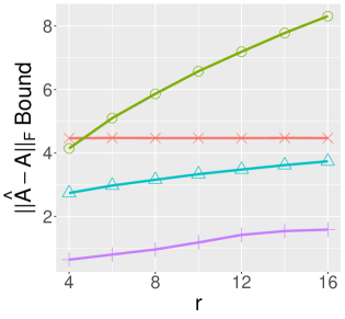
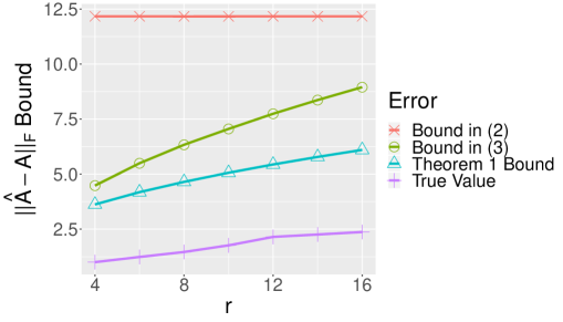
We first compare the low-rank matrix estimation error bound $\|\widehat{\mathbf{A}}-{\mathbf{A}}\|_{q}$ in Theorem 1 and the bounds in (2) and (3). We set $n\in\{100,300\},r\in\{4,6,\ldots,16\}$, $\sigma=0.02$, and generate ${\mathbf{A}}={\mathbf{U}}\boldsymbol{\Sigma}_{1}{\mathbf{V}}^{\top}$, where ${\mathbf{U}}\in\mathbb{R}^{n\times r},{\mathbf{V}}\in\mathbb{R}^{n\times r}$ are independently drawn from $\mathbb{O}_{n,r}$ uniformly at random; $\boldsymbol{\Sigma}_{1}$ is a diagonal matrix with singular values decaying polynomially as: $(\boldsymbol{\Sigma}_{1})_{[i,i]}=\frac{10}{i}$, $1\leq i\leq r$.

The evaluations of the upper bounds in Theorem 1, (2), (3), and the true value of $\|\widehat{{\mathbf{A}}}-{\mathbf{A}}\|_{F}$ are given in Figure 1. It shows that the upper bound in Theorem 1 is tighter than the upper bounds in (2), (3) in all settings. In addition, when $n$ increases from $100$ to $300$, the upper bound of (2) significantly increases while the upper bound of Theorem 1 remains steady. This is because the upper bounds of (2) and Theorem 1 rely on $\|{\mathbf{Z}}\|_{F}$ and $\|{\mathbf{Z}}_{\max(r)}\|_{F}$, respectively.

(a) $n=100$

(b) $n=300$

Figure 1: Low-rank matrix estimation error bound (Theorem 1), upper bounds (2), (3) and the true value of $\|\widehat{{\mathbf{A}}}-{\mathbf{A}}\|_{F}$

5.2 Numerical Comparison of Matrix Perturbation Projection Error Bounds

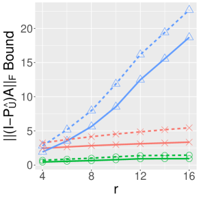
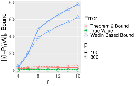
Next, we compare the matrix perturbation projection error bound in Theorem 2 with the upper bound (15) derived from Wedin’s sin$\Theta$ Theorem. We generate ${\mathbf{B}},{\mathbf{Z}}$ in the same way as the previous simulation setting. When generating $\boldsymbol{\Sigma}_{1}$ in ${\mathbf{A}}$, apart from the polynomial singular value decaying pattern considered in the last setting, we also consider the following exponential singular value decaying pattern: $(\boldsymbol{\Sigma}_{1})_{[i,i]}=2^{5-i}$, $1\leq i\leq r$.

The values of the upper bounds in Theorem 2 and (15), along with the true value of $\|P_{\widehat{{\mathbf{U}}}_{\perp}}{\mathbf{A}}\|_{q}$, are presented in Figure 2. We find the bound of Theorem 2 is much tighter than the bound in (15). As $r$ increases or singular value decaying pattern becomes exponential, i.e., ${\mathbf{A}}$ becomes ill-conditioned, (15) becomes loose while Theorem 2 can still be sharp.

(a) Singular values of ${\mathbf{A}}$ decay polynomially

(b) Singular values of ${\mathbf{A}}$ decay exponentially

Figure 2: Matrix perturbation projection error upper bound (Theorem 2), upper bound via Wedin’s sin$\Theta$ Theorem (15), and the true value of $\|P_{\widehat{\mathbf{U}}_{\perp}}{\mathbf{A}}\|_{F}$.

6 Discussions

In this paper, we prove a sharp upper bound for estimation error of rank-$r$ truncated SVD ($\|\widehat{\mathbf{A}}-{\mathbf{A}}\|_{q}$) under perturbation, and show its optimality in low-rank matrix estimation. The key technical tool we use is a novel matrix perturbation projection error bound for $\|P_{\widehat{{\mathbf{U}}}_{\perp}}{\mathbf{A}}\|_{q}$. As a byproduct, we also provide a sharper user-friendly sin$\Theta$ perturbation bound. The numerical studies demonstrate the advantages of these new results over the ones in the literature.

The main result of this paper is the upper bound in (4), which is sharper than ones directly derived from the literature (1), (2), (3). We also comment that (1) can be conveniently extended to the general case that ${\mathbf{A}}$ is approximately rank $r$ [Wed72, Eq.(4.4)]. It is interesting future work to study if a similar bound to (4) can be obtained for the general approximately low-rank ${\mathbf{A}}$.

Throughout the paper, we study the additive perturbations and it is a future work to extend the results to multiplicative perturbations [Li98a, Li98b]. Also for convenience of presentation, we focus on the real number field in this paper. It is interesting to extend the developed results to the field of complex numbers. The main technical work for such an extension includes complex versions of Lemma 2 and 3.

Apart from the widely studied perturbation theory on singular value decomposition, the perturbation theory for other problems, such as pseudo-inverses [Wed73, Ste77], least squares problems [Ste77], orthogonal projection [Ste77, Xu20, FB96, CCL16], rank-one perturbation [ZPL19], are also important topics. It would be interesting to explore whether the tools developed in this paper is useful in studying the perturbation theory for these problems.

References

- [BD90] Jesse Barlow and James Demmel. Computing accurate eigensystems of scaled diagonally dominant matrices. SIAM Journal on Numerical Analysis, 27(3):762–791, 1990.
- [BH88] Rajendra Bhatia and John AR Holbrook. On the Clarkson-McCarthy inequalities. Mathematische Annalen, 1988.
- [Bha13] Rajendra Bhatia. Matrix analysis, volume 169. Springer Science & Business Media, 2013.
- [CCL16] Yan Mei Chen, Xiao Shan Chen, and Wen Li. On perturbation bounds for orthogonal projections. Numerical Algorithms, 73(2):433–444, 2016.
- [CTP19] Joshua Cape, Minh Tang, and Carey E Priebe. The two-to-infinity norm and singular subspace geometry with applications to high-dimensional statistics. The Annals of Statistics, 47(5):2405–2439, 2019.
- [CZ18] T Tony Cai and Anru Zhang. Rate-optimal perturbation bounds for singular subspaces with applications to high-dimensional statistics. The Annals of Statistics, 46(1):60–89, 2018.
- [DG14] David Donoho and Matan Gavish. Minimax risk of matrix denoising by singular value thresholding. The Annals of Statistics, 42(6):2413–2440, 2014.
- [DK70] Chandler Davis and William Morton Kahan. The rotation of eigenvectors by a perturbation. III. SIAM Journal on Numerical Analysis, 7(1):1–46, 1970.
- [DK90] James Demmel and William Kahan. Accurate singular values of bidiagonal matrices. SIAM Journal on Scientific and Statistical Computing, 11(5):873–912, 1990.
- [DV92] James Demmel and Kresimir Veselić. Jacobi’s method is more accurate than QR. SIAM Journal on Matrix Analysis and Applications, 13(4):1204–1245, 1992.
- [DV08] Zlatko Drmac and Kresimir Veselić. New fast and accurate Jacobi SVD algorithm. I. SIAM Journal on matrix analysis and applications, 29(4):1322–1342, 2008.
- [EY36] Carl Eckart and Gale Young. The approximation of one matrix by another of lower rank. Psychometrika, 1(3):211–218, 1936.
- [FB96] Ricardo D Fierro and James R Bunch. Perturbation theory for orthogonal projection methods with applications to least squares and total least squares. Linear Algebra and Its Applications, 234:71–96, 1996.
- [GD14] Matan Gavish and David L Donoho. The optimal hard threshold for singular values is . IEEE Transactions on Information Theory, 60(8):5040–5053, 2014.
- [GHS87] Gene H Golub, Alan Hoffman, and Gilbert W Stewart. A generalization of the Eckart-Young-Mirsky matrix approximation theorem. Linear Algebra and Its Applications, 88:317–327, 1987.
- [Ips00] Ilse CF Ipsen. An overview of relative sin theorems for invariant subspaces of complex matrices. Journal of Computational and Applied Mathematics, 123(1-2):131–153, 2000.
- [Jol02] Ian Jolliffe. Principal component analysis. Springer, New York, 2nd ed. edition, 2002.
- [Li98a] Ren-Cang Li. Relative perturbation theory: I. eigenvalue and singular value variations. SIAM Journal on Matrix Analysis and Applications, 19(4):956–982, 1998.
- [Li98b] Ren-Cang Li. Relative perturbation theory: II. eigenspace and singular subspace variations. SIAM Journal on Matrix Analysis and Applications, 20(2):471–492, 1998.
- [LLM08] Jun Liu, Xiangqian Liu, and Xiaoli Ma. First-order perturbation analysis of singular vectors in singular value decomposition. IEEE Transactions on Signal Processing, 56(7):3044–3049, 2008.
- [LR00] Tristan Londré and Noah H Rhee. A note on relative perturbation bounds. SIAM Journal on Matrix Analysis and Applications, 21(2):357–361, 2000.
- [LR15] Jing Lei and Alessandro Rinaldo. Consistency of spectral clustering in stochastic block models. The Annals of Statistics, 43(1):215–237, 2015.
- [Mir60] Leon Mirsky. Symmetric gauge functions and unitarily invariant norms. The Quarterly Journal of Mathematics, 11(1):50–59, 1960.
- [MMS76] Donald F Morrison, Lauriston C Marshall, and Harry L Sahlin. Multivariate statistical methods. McGraw-Hill New York, 1976.
- [SS90] Gilbert W Stewart and Ji-Guang Sun. Matrix perturbation theory, 1990.
- [Ste77] Gilbert W Stewart. On the perturbation of pseudo-inverses, projections and linear least squares problems. SIAM Review, 19(4):634–662, 1977.
- [Ste06] Michael Stewart. Perturbation of the SVD in the presence of small singular values. Linear Algebra and Its Applications, 419(1):53–77, 2006.
- [TS93] Donald W Tufts and Abhijit A Shah. Estimation of a signal waveform from noisy data using low-rank approximation to a data matrix. IEEE Transactions on Signal Processing, 41(4):1716–1721, 1993.
- [UT19] Madeleine Udell and Alex Townsend. Why are big data matrices approximately low rank? SIAM Journal on Mathematics of Data Science, 1(1):144–160, 2019.
- [Vac94] Richard J Vaccaro. A second-order perturbation expansion for the SVD. SIAM Journal on Matrix Analysis and Applications, 15(2):661–671, 1994.
- [VL13] Vincent Q Vu and Jing Lei. Minimax sparse principal subspace estimation in high dimensions. The Annals of Statistics, 41(6):2905–2947, 2013.
- [Wed72] Per-Ake Wedin. Perturbation bounds in connection with singular value decomposition. BIT Numerical Mathematics, 12(1):99–111, 1972.
- [Wed73] Per-Ake Wedin. Perturbation theory for pseudo-inverses. BIT Numerical Mathematics, 13(2):217–232, 1973.
- [Wey12] Hermann Weyl. Das asymptotische verteilungsgesetz der eigenwerte linearer partieller differentialgleichungen (mit einer anwendung auf die theorie der hohlraumstrahlung). Mathematische Annalen, 71(4):441–479, 1912.
- [Xu02] Zhengyuan Xu. Perturbation analysis for subspace decomposition with applications in subspace-based algorithms. IEEE Transactions on Signal Processing, 50(11):2820–2830, 2002.
- [Xu20] Xuefeng Xu. On the perturbation of an -orthogonal projection. Journal of Computational and Applied Mathematics, 368:112327, 2020.
- [YWS15] Yi Yu, Tengyao Wang, and Richard J Samworth. A useful variant of the Davis–Kahan theorem for statisticians. Biometrika, 102(2):315–323, 2015.
- [ZPL19] Lei Zhu, Xiaofei Peng, and Hao Liu. Rank-one perturbation bounds for singular values of arbitrary matrices. Journal of Inequalities and Applications, 2019(1):138, 2019.