A User Guide to Low-Pass Graph Signal Processing and its Applications
Abstract
The notion of graph filters can be used to define generative models for graph data. In fact, the data obtained from many examples of network dynamics may be viewed as the output of a graph filter. With this interpretation, classical signal processing tools such as frequency analysis have been successfully applied with analogous interpretation to graph data, generating new insights for data science. What follows is a user guide on a specific class of graph data, where the generating graph filters are low-pass, i.e., the filter attenuates contents in the higher graph frequencies while retaining contents in the lower frequencies. Our choice is motivated by the prevalence of low-pass models in application domains such as social networks, financial markets, and power systems. We illustrate how to leverage properties of low-pass graph filters to learn the graph topology or identify its community structure; efficiently represent graph data through sampling, recover missing measurements, and de-noise graph data; the low-pass property is also used as the baseline to detect anomalies.
I Introduction
A growing trend in signal processing and machine learning is to develop theories and models for analyzing data defined on irregular domains such as graphs. Graphs often express relational ties, such as social, economics networks, or gene networks, for which several mathematical and statistical models relying on graphs have been proposed to explain trends in the data [1]. Another case is that of physical infrastructures (utility networks such as power, gas, water delivery systems and transportation networks) where physical laws, in addition to the connectivity, define the structure in signals.
For a period of time, the graphical interpretation was primarily used in statistics with the aim of making inference about graphical models. Meanwhile, the need for processing graph data has led to the emerging field of graph signal processing (GSP), which takes a deterministic and system theoretic approach to justify the properties of graph data and to inspire the associated signal processing algorithms. A cornerstone of GSP is the formal definition of graph filter, which extends the notions of linear time invariant (LTI) filtering of time series signals to data defined on a graph, a.k.a. graph signals.
In a similar vein as LTI filters in discrete-time signal processing, a graph filter can be classified as either low-pass, band-pass, or high-pass, depending on its graph frequency response. Among them, this article focuses on the low-pass graph filters and the low-pass graph signals generated from them. These graph filters capture a smoothing operation applied to the input graph signals, which is a common property of processes observed in many physical/social systems (see Section III). As a motivating example, in Fig. 1, we illustrate a few real datasets with such models from social networks, power systems and financial market, and show the eigenvalue spectra of their sample covariance matrices. A salient feature observed is that these sample covariance matrices are low-rank, thus displaying an important symptom of low-pass filtered graph signals (to be discussed in Section IV).
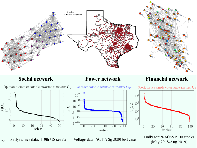
Previous articles such as [2, 3] have provided a comprehensive introduction to modeling and processing graph or network data using GSP, favoring general abstractions over focusing on particular structures and concrete applications. This user guide takes a different approach, concentrating on low-pass graph filters and the corresponding low-pass graph signal outputs. Low-pass graph signals have specific properties that affect their structure and dictate how to approach, for example, sampling, denoising and inference problems. They are worth focusing on, because they are very common in practice. We start the article by surveying low-pass GSP properties and insights, setting the stage for the description of the concrete situations where such a model applies. A set of particular examples is then provided, highlighting the fact that low-pass graph signals often appear in different application domains. In fact, resorting to existing underlying network dynamical models that justify different data sets, we show that low-pass graph processes are nearly ubiquitous in contexts where GSP is applicable.
II Basics of Graph Signal Processing
Many tools introduced in this user guide involve several fundamental concepts of GSP, including a formal definition of low-pass graph filters/signals. These ideas will be briefly reviewed in this section. For more details, the readers are referred to the excellent prior overview articles such as [3, 2]. We denote vectors with boldfaced lowercase letters, and uppercase letters for matrices, . The operation creates a diagonal matrix with elements from vector .
We focus on a weighted undirected graph with nodes such that and is the edge set. A graph signal is a function which can be represented by a -dimensional vector . A Graph Shift Operator (GSO) is a matrix satisfying if and only if or . When multiplied by a graph signal , each entry of the shifted graph signal is a linear combination of the one-hop neighbors’ values, therefore ‘shifting’ the graph signal with respect to the graph topology. In this article, we take the Laplacian matrix as the GSO. The Laplacian matrix is defined as , where is the weighted symmetric adjacency matrix of , and is a diagonal matrix of the weighted degrees. It is also common to take the GSO as the normalized Laplacian matrix, or the adjacency matrix [4].
Having defined the GSO, we discuss how to measure the smoothness of graph signals and analyze their content in the graph frequency domain. Recall that if a signal is smooth in time, the norm of its time derivative is small. For a graph signal , its graph derivative is defined as
The squared Frobenius norm of graph derivative, a.k.a. the graph quadratic form [2], provides an idea of the smoothness of the graph signal :
| (1) |
Observe that if for any neighboring nodes , then . As such, we say that a graph signal is smooth if is small.
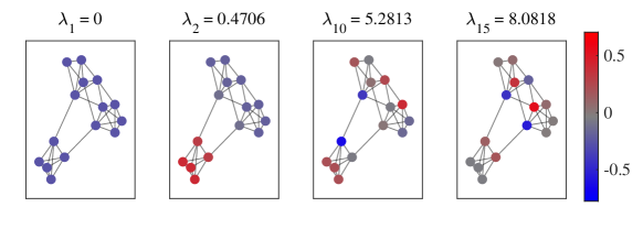
Let us take a closer look at the graph quadratic form . We set the eigendecomposition of the Laplacian matrix as and assume that it has eigenvalues of multiplicity one ordered as with , and with being the eigenvector for . Observe that for any , it holds , and for any orthogonal to , it holds and so on for the other eigenvectors. The observation indicates that the larger the eigenvalue, the more oscillatory the eigenvector is over the vertex set. In particular, the smallest eigenvalue is associated with the flat, all-ones eigenvector , as seen in Fig. 2. The above motivates the definition of graph frequencies as the eigenvalues and of the Graph Fourier Transform (GFT) basis as the set of eigenvectors [4]. Therefore, the frequency component of is defined as the inner product between and :
| (2) |
and is called the GFT of . The magnitude of the GFT vector is the ‘spectrum’ of the graph signal , where represents the signal power at the th frequency.
An important concept to modelling data with GSP is the graph filtering operation. To this end, a linear graph filter is described as the linear operator:
| (3) |
where is the filter order (can be infinite) and are the filter’s coefficients; as a convention, we use and . From (3), one can see that the graph filter has similar interpretation as an LTI filter in discrete-time signal processing where the former replaces the time shifts by powers of the GSO. Meanwhile, the second expression in (3) defines the frequency response as the diagonal matrix . A graph signal is said to be filtered by with the input excitation when
| (4) |
To better appreciate the effects of the graph filter, note that the th frequency component of is:
| (5) |
where is the transfer function of the graph filter, or equivalently, we have . It is similar to the convolution theorem in discrete-time signal processing.
Low-pass Graph Filter and Signal
Inspired by (5), we define the ideal low-pass graph filter with a cut-off frequency through setting the transfer function as and otherwise [5]. Alternatively, one can say that a graph filter is low-pass if its frequency response is concentrated on the low graph frequencies. In this article, we adopt the following definition from [6]:
Definition 1.
For any , define the ratio
(6)
The graph filter is -low-pass if and only if the low-pass ratio satisfies .
The integer parameter characterizes the bandwidth, or the cut-off frequency of the low-pass filter is at . The ratio quantifies the ‘strength’ of the low-pass graph filter. Upon passing a graph signal through , the high frequency components (above ) are attenuated by a factor of less than or equal to . Using this definition, the ideal -low-pass graph filter has the ratio , whose filter order has to be at least and transfer function has as its roots.
Finally, a -low-pass graph signal refers to a graph signal that is the output of a -low-pass filter, subject to a ‘well-behaved’ excitation (i.e. does not possess strong high frequency components), which includes, but is not limited to, the white noise.
The Impact of Graph Topologies
From Definition 1, one can observe that the low-pass ratio of a graph filter depends on the filter’s coefficients and the graph Laplacian matrix’s spectrum . The condition facilitates the design of a -low-pass graph filter with a favorable ratio and a low filter order . As an example, the order-1 graph filter is -low-pass with the ratio , where is small if .
An example of graph topologies favoring the condition is the stochastic block model (SBM) [7] for describing random graphs with blocks/communities with nodes in partitioned as . Consider a simplified SBM with equal-sized blocks specified by a membership matrix such that if and only if ; and a latent model where is the probability of edges between nodes in block and . We consider the homogeneous planted partition model (PPM) such that with . With the above specification, the adjacency matrix is a symmetric binary matrix with independent entries satisfying . When the graph size grows to infinity (), the Laplacian matrix of an SBM-PPM graph converges almost surely to its expected value [7, Theorem 2.1]:
| (7) |
From the above, it can be shown that for , i.e., a favorable graph model for -low-pass graph filters. Lastly, the bottom- eigenvectors of the expected Laplacian associated with can be collected into the matrix , where diagonalizes the matrix . In other words, the eigenvectors corresponding to the bottom- eigenvalues of will reveal the block structure.
In contrast, the Erdös-Rényi graphs have Laplacian matrices that do not generally satisfy . In fact, asymptotically () the empirical distribution of the eigenvalues of Laplacian matrices tends to the free convolution of the standard Gaussian distribution and the Wigner’s semi-circular law [8]. Such spectrum does not favor the design of a -low-pass graph filter with , reflecting the fact that block structure or communities do not emerge in Erdös Rényi graphs.
Low-pass Graph-Temporal Filter
When the excitation to a graph filter is of time-varying nature, and the topology is fixed, we consider a graph-temporal filter [9] with the impulse response:
| (8) |
such that the graph filter’s output is given by the time-domain convolution . The filter is causal and for . We can apply -transform and the GFT to the graph signal process to obtain the -GFT signal, , given by:
| (9) |
which represents in the joint -graph frequency domain. With that, we obtain the input-output relation and graph-temporal joint transfer function . A class of graph-temporal filters for modeling graph signal processes is the GF-ARMA filter, whose input-output relation in time domain and -GFT domain are described below, respectively:
where and are the -transform of the graph frequency responses of the graph filter taps , for the GF-ARMA filter. Note that the joint frequency response is given by , whose poles and zeros may vary depending on the graph frequencies . A relevant case is when is a low-pass graph-temporal filter. Similar to Definition 1, we say that is low-pass with a cutoff frequency and ratio if:
| (10) |
Graph signals filtered by a low-pass graph-temporal filter are also commonly found in applications, as we will illustrate next.
III Models of Low-pass Graph Signals
Before studying the GSP tools for low-pass graph signals, a natural question is where can one find such graph signals? It turns out that many physical and social processes are naturally characterized by low-pass graph filters. In this section, we present various examples and show that their generation processes can be represented as outputs from low-pass graph filters.
Diffusion Model
The first case pertains to observations from a diffusion process, whose variants are broadly applicable in network science. As an example, we consider the heat diffusion model in [10]. In this example, the relevant graph is a proximity graph where each node is a location (e.g., cities), and if locations are close to each other, then . The graph is endowed with a symmetric weighted adjacency matrix encoding the distance between locations. The graph signal encodes the temperature of locations at time , and let be the initial heat distribution. The temperature of a location is diffused to its neighbors. Let be a constant, we have
| (11) |
where (11) is a discretization of the heat diffusion equation [10]. As , the matrix exponential is row stochastic. The temperature at time is thus a weighted average of neighboring locations’ temperatures at , i.e., this is a diffusion dynamical process.
To understand (11) under the context of low-pass filtering, we observe that is a filtered graph signal with the excitation and the graph filter . We verify that is -low-pass with Definition 1 for any . Note that the low-pass ratio is:
As and , we see that is a -low-pass graph filter for any .
We have assumed that is an impulse excitation affecting the system only at the initial time. In practice, the excitation signal may not be an impulse and the output graph signal is expressed as the convolution . This corresponds to a low-pass graph-temporal filter with the joint transfer function . Besides, the diffusion process is common in network science as similar models arise in contagion process and product adoption to name a few.
Opinion Dynamics
This example pertains to opinion data mined from social networks with the influence of external excitation [6, 11]. The relevant graph is the social network graph where each node is an individual, and is the set of friendships. Similar to the previous case study, this graph is endowed with a symmetric weighted adjacency matrix , where the weights measure the trust among pairs of individuals. Let , be parameters of trust on others and susceptibility to external influence of an individual respectively. The evolution of opinions follows that of a combination of DeGroot’s and Friedkin-Johnsen’s model [12], which is a GF-AR(1) model:
| (12) |
where is a graph signal of the individuals’ opinions at time , and is a graph signal of the external opinions perceived by the social network. Note that this also corresponds to a low-pass graph-temporal filter with the joint transfer function .
To discuss the steady state of (12), let us assume that . Considering (12), we observe that is a convex combination of and weighted average of the neighbors’ opinions at time that is formed by taking a weighted average of neighboring signals in using a diffusion operator . As , the recursion is stable, leading to the steady state (or equilibrium) opinions:
| (13) |
where we have defined and is a filtered graph signal excited by .
The graph filter above is given by . To verify that it is a -low-pass graph filter with Definition 1, we note that for any , the low-pass ratio is
Again, we observe that as , the above graph filter is -low-pass for any . However, we remark that this low-pass ratio may be undesirable with when . Interestingly, a similar generative model as (12) is found in equilibrium problems such as quadratic games [13].
Two remarks are in order. First, social networks are typically directed, and this suggests using a non-symmetric shift operator as opposed to the symmetric Laplacian matrix, which we used for simplicity of exposition. Second, many alternative models for social networks interactions are non-linear and linear GSP is insufficient in those contexts.
Finance Data
Financial systems such as stock market and hedge funds produce return reports periodically about their business performances. A collection of these reports can be studied as graph signals, where the relevant graph consists of nodes that are financial institutions, and edges that are business ties between them. It has been studied [14] that business performances are correlated according to the business ties. Moreover, the returns are affected by a number of common factors [15]. Inspired by [14], [15, Ch. 12.2], let be the strength of external influences, a reasonable model for the transient dynamics of the graph signal of business performance measures is also a GF-AR(1):
| (14) |
where is an unknown but low-pass graph filter, represents the factor model affecting financial institutions, and is the excitation strength. The equilibrium of (14) is:
where . We see that is the excitation signal and the equilibrium is the filter output. Suppose that is a -low-pass graph filter with the frequency response satisfying , then for , we can evaluate the low-pass ratio as
As since is a -low-pass graph filter itself, we observe that is again -low-pass according to Definition 1.
For to be a -low-pass graph signal, one has to also assume that is not high-pass (i.e., not orthogonal to a low-pass one). This is a mild assumption as the latent factor affecting financial institutions are either independent of the network, or are aligned with the communities. Above all, we remark that (14) is an idealized model where determining the exact model is an open problem in economics, see [15, 14].
Power Systems
In the case of power systems, the relevant graph is the electrical transmission lines network. The node (a.k.a. bus) set includes generator buses, , and non-generator/load buses, . The edge set refers to the transmission lines connecting the buses. The branch admittance matrix, , models the effect of transmission lines and is a complex symmetric matrix associated with , where is the complex admittance of the branch between nodes and provided that . The graph signals we consider are the complex voltage phasors, denoted as when measured at time . They can be obtained using phasor measurement units (PMU) [16] installed on each bus . The graph shift operator in this case is a diagonally perturbed branch admittance matrix:
| (15) |
where is the generator admittance and is the load admittance at .
Note that is a GSO on the grid graph as if . The complex symmetric matrix can be decomposed as , where is a complex orthogonal matrix satisfying , and is a diagonal matrix with diagonal elements sorted as ; see [17] for modeling details. Let be the outgoing current at each node at time , given by where elements in are the internal voltage phasors at the generator buses. Applying Kirchoff’s current law in quasi-steady state, the voltage phasors are:
| (16) |
where captures the slow time-varying nature of the load and other modeling approximations. In other words, is a graph signal obtained by the graph filter and the excitation signal . Particularly, we observe that is a low-pass graph filter. Consider any , the low-pass ratio is
As the power grids tend to be organized as communities to serve different areas with high population densities, the system admittance matrix is block diagonal and sparse. In particular, with communities in the grid graph, these facts indicate that the graph filter is -low-pass satisfying .
The excitation graph signal itself has a low-rank structure, as at . The temporal dynamics of can be described as an AR(2) graph filter [9] using a reduced generator-only shift operator with the graph-temporal transfer function, ,
where is the stochastic power input to the system. The graph-temporal filter is low-pass in the time domain. The overall system in (16) has approximately the properties of a low-pass graph temporal filter according to the definition in (10).
IV User Guide to Low-pass Graph Signal Processing
If we observe a set of low-pass graph signals such as those from Section III, what can we learn from these signals? Can we find efficient representations for them? Can we exploit this structure to denoise the signal or detect anomalies? To answer these questions, we begin by studying two salient features of low-pass graph signals, namely low-rank covariance matrix, and smoothness as measured by the graph quadratic form. Then, we illustrate how these features can enable low-pass GSP to sample graph signals (and therefore compress them), to infer the graph topology, and to detect anomalous activities. Furthermore, when the graph topology admits a clustered structure, we highlight how these clusters emerge in the low-pass graph signals and provide insights on the optimal sampling patterns.
We now consider a set of low-pass graph signals that can be modeled as outcomes of independent and identically distributed random experiments, given as:
| (17) |
such that is a -low-pass graph filter defined on the Laplacian matrix, is the excitation signal, and is an additive noise. For simplicity, we do not consider the more general low-pass graph-temporal processes and assume that , are zero-mean white noise with , . We remark that the following observations still hold for the general setting when is not white, or even diagonal. The latter relaxation is important for the applications listed in Section III. For instance, in opinion dynamics, the excitation signals may represent external opinions that do not affect the social network uniformly, e.g., they are news articles written in a foreign language.
IV-A Low-rank Covariance Matrix
From (17), it is straightforward to show that is zero-mean with the covariance matrix
| (18) |
Recall that is a -low-pass graph filter, if as defined in (6), the energy of will be concentrated in the top- diagonal elements. Therefore, when the noise variance is small (), the low-pass graph signals lie approximately in , a -dimensional subspace of .
a-i). Sampling Graph Signals
As the -low-pass graph signals lie approximately in , it is possible to map the graph signals almost losslessly onto -dimensional vectors. While the -dimensional representation can be obtained by projecting on the space spanned by , it is not necessary to do so. An alternative to generate this -dimensional representation is by decimating the graph signals.
| \addvbuffer[0cm 4.75cm](a) | 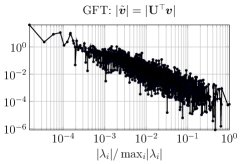 |
\addvbuffer[0cm 4.75cm](b) | 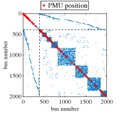 |
\addvbuffer[0cm 4.75cm](c) | 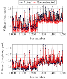 |
To describe the setup, we let be a sampling set with cardinality . A sampled version of is constructed as (omitting the subscript for brevity):
| (19) |
such that
and is a fat sampling matrix that compresses the graph signal to an -dimensional vector. To recover , we interpolate using a matching linear transformation [18], giving with to be designed later. Clearly, when , it is not possible to exactly recover an arbitrary graph signal. To ensure exact recovery, we see that it requires certain additional conditions on the sampling set and the graph signal.
Exactly recovering from its sampled version would require the sampled graph signal to be in the range space of sampling matrix . We let be the projection of onto the (low-frequency) subspace spanned by and be the projection error. The projected graph signal is a -bandlimited (in fact, -low-pass) graph signal. From [18, Theorem 1], a sufficient condition for exact recovery is that if
| (20) |
then there exists an interpolation matrix such that . In fact, it is possible to recover any -bandlimited graph signal from its sampled version. We have
| (21) |
As -low-pass graph signals lie approximately in , we have provided that . Under condition (20), the sampling-and-interpolation procedure results in a small interpolation error.
Clearly, a necessary condition to satisfy (20) is , i.e., we require at least the same number of samples as the bandwidth of the low-pass graph filter which produces the graph signal . Beyond the necessary condition, obtaining a sufficient condition for (20) can be difficult as it is not obvious to derive conditions on the sampling set. The design of the sampling set has been the focus of work in [18, 19, 20] which propose to find via a greedy method, or via the graph spectral proxies. The above statements are valid for any graph signal that has a sparse frequency support. In the case of low-pass graph signals, we can obtain insights on what type of sampling patterns are compatible with (20). Consider the special case of SBM-PPM graphs with blocks discussed in Section II. Note that as , we have for this model, where is the block-membership matrix. Subsequently, condition (20) can be easily verified if contains at least one node from each of the blocks.
In Fig. 3, we consider a power system application. We first plot the magnitude of GFT of voltage graph signal with respect to normalized graph frequencies in log scale. From the linear decay, it is evident that the magnitude of GFT coefficients at lower frequencies is higher confirming the signal is low-pass in nature. Then, the sampling pattern (or optimal placement of sensors) for graph signal reconstruction is shown in the figure. The block structure in the GSO for the electric grid guides the sampling strategy. In this example, the smallest singular value of is maximized using a greedy algorithm [20].
a-ii). Blind Community Detection
Another consequence of (18) relates to learning the block or community structure when the graph topology is unknown. When the graph topology is known, spectral clustering (SC) is often the method of choice. The SC method computes the bottom- eigenvectors of Laplacian as and partitions the nodes via -means:
| (22) |
where
such that is the th row vector of . In fact, this is an effective method for SBM-PPM graphs where solving (22) reveals the true block membership [7].
| \addvbuffer[0cm 5cm](a) | 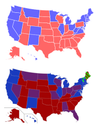 |
\addvbuffer[0cm 5cm](b) | 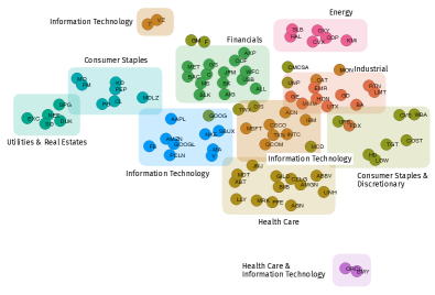
|
|---|
Although only the graph signals are observed, we know from (18) that the covariance matrix will be dominated by a rank- component spanned by under the low-pass assumption. In fact, this is precisely what we need for community detection as hinted in (22). To this end, [6] proposed the blind community detection (BlindCD) procedure:
If we denote the detected communities as , then
| (23) |
In other words, the BlindCD approaches the performance of SC if the graph filter is -low-pass with , the observation noise is small, and the number of samples is large. Notice that (23) is a general result which holds even if is non-diagonal or low-rank. Moreover, BlindCD is shown to outperform a two-step approach that learns the graph first and then apply SC; see [6].
In Fig. 4, we illustrate results of community detection for opinion dynamics and financial data by using data from US Senate from the 115th US Congress (2017-2019) and daily return data of stocks in the S&P100 index from Feb. 2013 to Dec. 2016 [source: https://www.kaggle.com/camnugent/sandp500] respectively. The observed steady-state graph signals for the opinion dynamics case are the aggregated vote records of each state, and we observe voting rounds. In Fig. 4 (a), we apply BlindCD to partition the states into groups, where a close alignment between our results with the actual party memberships of this US Congress is observed. The financial dataset used contains days of data for stocks. In Fig. 4 (b) we apply BlindCD to partition the stocks into groups. Each of the community detected includes companies of the same business type (for instance, ‘BAC’ (Bank of America) is with ‘JPM’ (JP Morgan)) showing the effectiveness of the method.
IV-B Smooth Graph Signals
In Section II we introduced the graph quadratic form to quantify the smoothness of a graph signal. Particularly, if , the graph signal is said to be smooth. For -low-pass graph signals, we observe that
| (24) |
where we have used that is -low-pass with to derive the approximations. In the cases when , such as large SBM-PPM graphs with parameters satisfying , , we expect the -low-pass graph signal to be smooth, i.e., .
b-i). Graph Topology Learning
The smoothness property can be used to learn the graph topology by fitting a Laplacian matrix which best smoothens the graph signals. This is exemplified by the estimator:
| (25) |
where we have used the graph quadratic form, , to regulate the smoothness of with respect to the fitted . Dong et al. [21] motivated (25) as a maximum-a-posterior (MAP) estimator for the Laplacian matrix, where and is the pseudo-inverse of the Laplacian matrix. This amounts to interpreting the data as outcomes of a Gaussian Markov Random Field (GMRF) with precision matrix chosen as the Laplacian, effectively connecting statistical graphical models to GSP models. Note that methods following similar insights as (25) can be found in [22, 23].
For graph signals that are output from low-pass graph temporal filters, a similar smoothness property to (24) can also be exploited to interpolate missing data. Let be a matrix whose columns are , where is the graph signal at time ; and be the sampled version of where some values are missing at different node/time indices. The key for interpolating the data is to regularize via graph quadratic form and norm of the time derivative in addition to minimizing the misfit between available samples and reconstructed samples at known locations, , i.e.,
See [24] and the references therein for a detailed discussion.
IV-C Anomalies Detection with Low-pass GSP
Consider a model consistent with (17). The fact that the low-pass graph process is dominated by low graph frequency components can be considered the null-hypothesis characterized by the low-pass properties, such as low-rank covariance matrix and smoothness. On the other hand, many anomalies can be modeled as an additive sparse noise signal , or a high frequency graph signal. Such noise signals arise in several scenarios such as a change in the graph connectivity or parameters, a contingency in infrastructures, the result of malicious activities in social networks, or the sudden fall in the market value of a financial entity. High frequency noise signals are also produced by a perturbation that is inconsistent with the generative model. For instance, in infrastructure networks this could be symptomatic of malfunctioning sensors or even a false data injection attack (FDIA)[25].
Such anomalies cause a surge in the high frequency spectral components of a low-pass graph signal, a fact that can be leveraged in a manner similar to the classical array processing problem of detecting a source embedded in noise.
| \addvbuffer[0cm 4.75cm](a) | 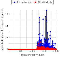 |
\addvbuffer[0cm 4.75cm](b) | 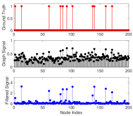 |
Formally, the observed signal under null and alternative hypothesis is described as
where is a high frequency graph signal. Our task amounts to testing the hypothesis , , and/or to estimate the locations of non-zeros in when the latter is a sparse signal and under .
Intuitively, we can apply a high-pass graph filter to distinguish between and . Let be an ideal high-pass graph filter with the frequency response , and otherwise. Consider the test statistics as . Under and the -low-pass assumption, we have , and thus the test statistics will be small. On the other hand, under , we obtain since the anomalies consist of high graph frequency components. Thus the test statistics will be large. Imposing a threshold of , we can consider the detector
Furthermore, if holds, these anomaly events can be located from the support of .
As a demonstration, Fig. 5 (a) shows the magnitude of GFT of the voltage graph signal after filtering using an ideal high-pass graph filter, . The voltage graph signal under the hypothesis of no anomaly is the output of a low-pass graph filter. When there is a FDIA, we observe an increase in energy of the high frequency components.
To obtain a simple implementation of high-pass graph filters, we may consider whose frequency response is given by . When applied on a graph signal , we will observe the difference between and , where the latter is a one-hop averaged version of . We call this operation the spatial difference which is similar to the method proposed in [26] for anomaly detection on social networks. See the illustration in Fig. 5 (b).
V Concluding Remarks
In this user guide, we highlighted the key elements of low-pass GSP in several applications like graph parameter inference and graph signal sampling while emphasizing the intuition from time series analysis. We also discussed several physical models where low-pass GSP can be effectively used. However, the tools available for low-pass GSP are ever-expanding, and aid the discovery of new physical models where low-pass GSP can be applied. Additionally, there are several open research directions as discussed below.
Directed Graphs
Throughout this article, we have assumed that the observed data is supported on a graph topology which is undirected, and the shift operator (Laplacian matrix) is symmetric. This is clearly not a truthful model for a lot of real systems such as social and economics networks. The challenge of extending the existing GSP tools to directed graphs lies in defining the appropriate GFT basis. For instance, the properties of a circular shift matrix is what a directed shift operator should emulate.
Much of the prior research has focused on finding the appropriate GFT basis on directed graphs. The definition of frequency is again variational, but based on the norm of the difference between and vector and the shift operator of the corresponding graph does not have to be symmetric. More formally, the idea of smoothness is defined as where is the maximum eigenvalue of . This is the definition used in [4] for GFT on directed graphs, where the GSO is set as the adjacency matrix and the GFT is defined as such that is obtained from the Jordan decomposition of the adjacency matrix . Although is a basis, it is not orthogonal, so the Parseval’s identity does not hold since . That is not surprising since the norm of does not have the same physical interpretation of power spectral density that applies to signals whose support is time. A potential fix is studied in [27] which searches for the GFT basis that minimizes the directed total variation, also see [28]. Unfortunately the GFT basis does not admit a closed form solution.
The tools discussed in this article, such as sampling theory [18] and anomaly detection may still work for low-pass graph signals on directed graphs with minor adjustments. The challenge lies in the graph inference/learning methods since second-order statistics such as correlations are difficult to justify in directed graphs, where also the notion of community is ambiguous. A useful definition of community must first be studied before tools of GSP can be applied for community inference in directed graphs.
Low-pass Graph Signals in the Edge Space
An alternative form of graph signals are those that are defined on the edges. They can be defined as the function and the equivalent vector , which are useful for describing flows on graphs such as traffic in transportation network. As suggested in [29], the shift operator can be taken as the edge Laplacian , where is the node-to-edge incidence matrix. The null space of the edge Laplacian corresponds to the cyclic flow vector, which is also the eigenvector for the lowest graph frequency . It is anticipated that a low-pass edge-graph signal, whose energy is focused in the low graph frequencies, will consist of mostly cyclic flows within communities. An interesting direction is to develop a sampling theory for low-pass edge-graph signals, as well as the inference of edge Laplacian matrix.
Identifying Low-pass Graph Signals
So far we have relied on domain knowledge about the data models, e.g., the examples in Section III, to help justify various graph data as low-pass graph signals.
For graph signals taken from an unknown system, one has to be cautious before applying this low-pass GSP user guide. Even though non-low-pass graph processes are rarely found in a natural setting, there is a crucial need to design tools for identifying low-pass graph signals. With known GSO, it can be done by inspecting the GFT spectrum; with unknown GSO, the problem is related to the joint estimation of graph process and topology; readers are referred to [30] for recent works in this direction.
Acknowledgement
The authors thank the anonymous reviewers and the guest editors for their useful feedback. This material is based upon work supported in part by, the U. S. Army Research Laboratory and the U. S. Army Research Office under contract/grant number W911NF2010153 and the NSF CCF-BSF: CIF: 1714672 grant. Hoi-To Wai’s work is supported by the CUHK Direct Grant #4055135.
References
- [1] E. D. Kolaczyk and G. Csárdi, Statistical analysis of network data with R. Springer, 2014, vol. 65.
- [2] D. I. Shuman, S. K. Narang, P. Frossard, A. Ortega, and P. Vandergheynst, “The emerging field of signal processing on graphs: Extending high-dimensional data analysis to networks and other irregular domains,” IEEE Signal Processing Magazine, vol. 30, no. 3, pp. 83–98, 2013.
- [3] A. Ortega, P. Frossard, J. Kovačević, J. M. Moura, and P. Vandergheynst, “Graph signal processing: Overview, Challenges, and Applications,” Proceedings of the IEEE, vol. 106, no. 5, pp. 808–828, 2018.
- [4] A. Sandryhaila and J. M. Moura, “Discrete Signal Processing on Graphs,” IEEE Transactions on Signal Processing, vol. 61, no. 7, pp. 1644–1656, 2013.
- [5] N. Tremblay, P. Gonçalves, and P. Borgnat, “Design of Graph Filters and Filterbanks,” in Cooperative and Graph Signal Processing. Elsevier, 2018, pp. 299–324.
- [6] H.-T. Wai, S. Segarra, A. E. Ozdaglar, A. Scaglione, and A. Jadbabaie, “Blind Community Detection From Low-Rank Excitations of a Graph Filter,” IEEE Transactions on Signal Processing, vol. 68, pp. 436–451, 2020.
- [7] K. Rohe, S. Chatterjee, B. Yu et al., “Spectral clustering and the high-dimensional stochastic blockmodel,” The Annals of Statistics, vol. 39, no. 4, pp. 1878–1915, 2011.
- [8] X. Ding, T. Jiang et al., “Spectral distributions of adjacency and Laplacian matrices of random graphs,” The Annals of Applied Probability, vol. 20, no. 6, pp. 2086–2117, 2010.
- [9] E. Isufi, A. Loukas, A. Simonetto, and G. Leus, “Separable autoregressive moving average graph-temporal filters,” in 2016 24th European Signal Processing Conference (EUSIPCO). IEEE, 2016, pp. 200–204.
- [10] D. Thanou, X. Dong, D. Kressner, and P. Frossard, “Learning Heat Diffusion Graphs,” IEEE Transactions on Signal and Information Processing over Networks, vol. 3, no. 3, pp. 484–499, 2017.
- [11] C. Ravazzi, R. Tempo, and F. Dabbene, “Learning Influence Structure in Sparse Social Networks,” IEEE Transactions on Control of Network Systems, vol. 5, no. 4, pp. 1976–1986, 2017.
- [12] N. E. Friedkin, “A Formal Theory of Reflected Appraisals in the Evolution of Power,” Administrative Science Quarterly, vol. 56, no. 4, pp. 501–529, 2011.
- [13] O. Candogan, K. Bimpikis, and A. Ozdaglar, “Optimal Pricing in Networks with Externalities,” Operations Research, vol. 60, no. 4, pp. 883–905, 2012.
- [14] M. Billio, M. Getmansky, A. W. Lo, and L. Pelizzon, “Econometric measures of connectedness and systemic risk in the finance and insurance sectors,” Journal of financial economics, vol. 104, no. 3, pp. 535–559, 2012.
- [15] R. N. Mantegna and H. E. Stanley, Introduction to econophysics: correlations and complexity in finance. Cambridge university press, 1999.
- [16] J. D. Glover, M. Sarma, and T. Overbye, “Power System Analysis and Design,” Cengage Learning, vol. 4, 2008.
- [17] R. Ramakrishna and A. Scaglione, “On Modeling Voltage Phasor Measurements as Graph Signals,” in 2019 IEEE Data Science Workshop, DSW 2019. Institute of Electrical and Electronics Engineers Inc., 2019, pp. 275–279.
- [18] S. Chen, R. Varma, A. Sandryhaila, and J. Kovačević, “Discrete Signal Processing on Graphs: Sampling Theory,” IEEE Transactions on Signal Processing, vol. 63, no. 24, pp. 6510–6523, 2015.
- [19] A. Anis, A. Gadde, and A. Ortega, “Efficient Sampling Set Selection for Bandlimited Graph Signals Using Graph Spectral Proxies,” IEEE Transactions on Signal Processing, vol. 64, no. 14, pp. 3775–3789, 2016.
- [20] M. Tsitsvero, S. Barbarossa, and P. Di Lorenzo, “Signals on graphs: Uncertainty Principle and Sampling,” IEEE Transactions on Signal Processing, vol. 64, no. 18, pp. 4845–4860, 2016.
- [21] X. Dong, D. Thanou, P. Frossard, and P. Vandergheynst, “Learning Laplacian Matrix in Smooth Graph Signal Representations,” IEEE Transactions on Signal Processing, vol. 64, no. 23, pp. 6160–6173, 2016.
- [22] V. Kalofolias, “How to Learn a Graph from Smooth Signals,” in Artificial Intelligence and Statistics, 2016, pp. 920–929.
- [23] B. Pasdeloup, V. Gripon, G. Mercier, D. Pastor, and M. G. Rabbat, “Characterization and Inference of Graph Diffusion Processes From Observations of Stationary Signals,” IEEE Transactions on Signal and Information Processing over Networks, vol. 4, no. 3, pp. 481–496, 2017.
- [24] F. Grassi, A. Loukas, N. Perraudin, and B. Ricaud, “A Time-Vertex Signal Processing Framework: Scalable Processing and Meaningful Representations for Time-Series on Graphs,” IEEE Transactions on Signal Processing, vol. 66, no. 3, pp. 817–829, 2017.
- [25] R. Ramakrishna and A. Scaglione, “Detection of False Data Injection Attack using Graph Signal Processing for the Power Grid,” in 2019 IEEE Global Conference on Signal and Information Processing (GlobalSIP). Institute of Electrical and Electronics Engineers Inc., 2019, pp. 1–5.
- [26] H.-T. Wai, A. E. Ozdaglar, and A. Scaglione, “Identifying Susceptible Agents in Time Varying Opinion Dynamics Through Compressive Measurements,” in 2018 IEEE International Conference on Acoustics, Speech and Signal Processing (ICASSP). IEEE, 2018, pp. 4114–4118.
- [27] S. Sardellitti, S. Barbarossa, and P. Di Lorenzo, “On the Graph Fourier Transform for Directed Graphs,” IEEE Journal of Selected Topics in Signal Processing, vol. 11, no. 6, pp. 796–811, 2017.
- [28] R. Shafipour, A. Khodabakhsh, G. Mateos, and E. Nikolova, “A Directed Graph Fourier Transform With Spread Frequency Components,” IEEE Transactions on Signal Processing, vol. 67, no. 4, pp. 946–960, 2018.
- [29] M. T. Schaub and S. Segarra, “Flow smoothing and denoising: graph signal processing in the edge-space,” in 2018 IEEE Global Conference on Signal and Information Processing (GlobalSIP). IEEE, 2018, pp. 735–739.
- [30] V. N. Ioannidis, Y. Shen, and G. B. Giannakis, “Semi-Blind Inference of Topologies and Dynamical Processes Over Dynamic Graphs,” IEEE Transactions on Signal Processing, vol. 67, no. 9, pp. 2263–2274, 2019.