Dynamical state for 964 galaxy clusters from Chandra X-ray images

Abstract

The dynamical state of galaxy clusters describes if clusters are relaxed dynamically or in a merging process of subclusters. By using archival images from the Chandra X-ray Observatory, we derive a set of parameters to describe the dynamical state for 964 galaxy clusters. Three widely used indicators for dynamical state, the concentration index $c$, the centroid shift $\omega$ and the power ratio $P_{3}/P_{0}$ are calculated in the circular central region with a radius of 500 kpc. We also derive two adaptive parameters, the profile parameter $\kappa$ and the asymmetry factor $\alpha$, in the best fitted elliptical region. The morphology index $\delta$ is then defined by combining these two adaptive parameters, which indicates the dynamical state of galaxy clusters and has good correlations to the concentration index $c$, the centroid shift $\omega$, the power ratio $P_{3}/P_{0}$, and the optical relaxation factor $\Gamma$. For a large sample of clusters, the dynamical parameters are continuously distributed from the disturbed to relaxed states with a peak in the between, rather than the bimodal distribution for the two states. We find that the newly derived morphology index $\delta$ works for the similar fundamental plane between the radio power, cluster mass and the dynamical state for clusters with diffuse radio giant-halos and mini-halos. The offset between masses estimated from the Sunyaev-Zeld́ovich effect and X-ray images depends on dynamical parameters. All dynamical parameters for galaxy clusters derived from the Chandra archival images are available on http://zmtt.bao.ac.cn/galaxy_clusters/dyXimages/.

1 Introduction

In the hierarchical structure formation scenario, galaxy clusters are formed by continuous merging of smaller infalling groups and finally achieve dynamical equilibrium (e.g. Press & Schechter, 1974; McGee et al., 2009; Chiang et al., 2013). As the largest gravitational bound systems in the universe, clusters of galaxies consist of a large number of member galaxies embedded in the intracluster medium (ICM) and the dark matter halo. Often seen inside a galaxy cluster are the substructures in the spatial distribution of galaxies (e.g., Dressler & Shectman, 1988; Wen & Han, 2013). Because the hot gas in the ICM observed in the X-ray band is in kinematics equilibrium under the assumption of the energy density equipartition between the ICM and galaxies, many substructures have also been detected in the X-ray images (e.g., Kolokotronis et al., 2001).

The dynamical state of galaxy clusters describes if clusters are relaxed dynamically or are still in a merging process of subclusters. Clusters of galaxies are therefore broadly divided into relaxed clusters and dynamically disturbed clusters. Relaxed clusters roughly reach the virial equilibrium, showing a symmetrical structure in the distribution of galaxies and the intracluster gas around their brightest cluster galaxy (BCG). While dynamically disturbed clusters, such as the Bullet cluster (Markevitch et al., 2002), obviously deviate from the virial equilibrium with subclusters around two or more very bright galaxies (e.g., Colless & Dunn, 1996; Barrena et al., 2002; Wen & Han, 2013) or clear substructures in X-ray images (e.g., Mohr et al., 1995; Maughan et al., 2008; Yu et al., 2016). The dynamical state of galaxy clusters is ideally expressed by the three-dimensional (3D) velocity distribution of member galaxies (e.g. Colless & Dunn, 1996; Einasto et al., 2010, 2012) or the ICM (e.g. Dupke & Bregman, 2006; Liu et al., 2015, 2016; Yu et al., 2016). In practice, the dynamical state can be roughly indicated by the 1D radial velocity or redshift distribution (e.g., Yahil & Vidal, 1977; Dressler & Shectman, 1988; West & Bothun, 1990; Solanes et al., 1999; Halliday et al., 2004; Hou et al., 2009; Roberts et al., 2018; Yu et al., 2018), or the 2D positions of member galaxies in the sky plane projected from their real spatial distribution (e.g., Geller & Beers, 1982; West & Bothun, 1990; Flin & Krywult, 2006; Ramella et al., 2007; Aguerri & Sánchez-Janssen, 2010; Einasto et al., 2012; Wen & Han, 2013; Lopes et al., 2018) or the projected hot gas distribution shown in X-ray or microwave-band images of clusters (e.g., Mohr et al., 1995; Kolokotronis et al., 2001; Bauer et al., 2005; Chon et al., 2012; Cialone et al., 2018).

Substructures in such a projected two dimensional distribution of member galaxies or hot gas have been parameterized quantitatively to describe the dynamical state of galaxy clusters, such as the asymmetric factors or the probability distribution based on the optical data (e.g. West & Bothun, 1990; Ramella et al., 2007; Wen & Han, 2013), or the concentration index (e.g., Mohr et al., 1995; Santos et al., 2008), the centroid shift (e.g., Mohr et al., 1995; Poole et al., 2006; Maughan et al., 2008) and the power ratio (e.g., Buote & Tsai, 1995, 1996; Böhringer et al., 2010) based on the data of the X-ray images, see details in Section 3.1.

Wen & Han (2013) derived relaxation parameters for 2092 rich clusters based on photometric data by using the asymmetry, the ridge flatness and the normalized deviation of the smoothed optical maps, which is the largest sample of clusters to our knowledge with dynamical parameters. Klein et al. (2019) found a good agreement between the galaxy density maps and the X-ray brightness maps, and therefore estimated the dynamical parameters for 890 clusters by the method given by Wen & Han (2013). Recently, Cialone et al. (2018) also tried to parameterize the morphological characterization of synthetic maps of the Sunyaev-Zeld́ovich (SZ) effect for a sample of 258 simulated clusters. Lopes et al. (2018) estimated optical substructure parameters for 72 clusters which have Chandra X-ray images and/or Planck Sunyaev-Zeld́ovich maps by using optical imaging and spectroscopic data. Rumbaugh et al. (2018) showed the close correlation between dynamical parameters (difference between the optical and X-ray center, the projected offset of the BCG from other cluster centroids) and the offset from the scaling relations for clusters. Zenteno et al. (2020) also calculated the offsets between BCGs and gas center as traced by SZ effect (SPT) and/or X-ray (Chandra and XMM-Newton) images as dynamical parameter for 288 massive clusters.

The dynamical parameters have been involved to many studies, e.g. the cosmological constraints based on galaxy clusters with different X-ray morphologies (e.g. Mohr et al., 1995), the evolution of galaxy clusters in the cosmological model of structure formation (e.g. Buote & Tsai, 1996), the presence of radio halos and relics in merging clusters and the formation of mini-halos in relaxed clusters (e.g., Cassano et al., 2010, 2013; Cuciti et al., 2015; Yuan et al., 2015), the mass estimation (e.g., Ribeiro et al., 2011) and radial mass profile (e.g., Bartalucci et al., 2019) for clusters of galaxies, the scaling relations for cluster mass estimations (e.g., O’Hara et al., 2006; Chen et al., 2007; Zhang et al., 2008; Zhao et al., 2013), the dynamical-state dependence of galaxy luminosity functions (e.g., Wen & Han, 2015), and activity of super massive black holes in BCGs (Kale et al., 2015; Yuan et al., 2016).

In fact, any definition of dynamical parameters may be biased because we cannot get the real 3D distribution and velocities. Nevertheless, the identification and analysis of substructures of any projected galaxy distribution or X-ray images should give the lower limit of dynamical parameters ideally derived from the unavailable real 3D distribution. Therefore, it is still valuable to get dynamical parameters from the X-ray images of galaxy clusters. The Chandra satellite has observed about 1000 clusters of galaxies in the X-ray band, and the high resolution Chandra image is ideally to reveal the substructures from the ICM. In this paper, we derive a set of dynamical parameters for 964 clusters based on the archival data of the Chandra X-ray Observatory.

Figure 1: Redshift distribution for 911 of 964 clusters with available redshift.

In Section 2, we describe how we get and process the Chandra data. In Section 3, we define and calculate various dynamical parameters. Comparison of the derived parameters and discussions on the impact of dynamical state on the scaling relations are presented in Section 4. A summary is given in Section 5. Throughout this paper, we assume a flat $\Lambda$CDM cosmology taking $H_{0}=70$ km s^-1 Mpc^-1, $\Omega_{m}=0.3$ and $\Omega_{\Lambda}=0.7$.

2 Data collection and processing

2.1 Chandra data for galaxy clusters

We collect the observation information for clusters of galaxies archived by the Chandra in two approaches.

First, we get the information for all observations which categorized as “Clusters of galaxies” in the Chandra archival database. As a result, more than 2000 observations are obtained, often several observations are made for one cluster. For clusters observed more than one time, we generally choose the observation with largest photon number. However, we select the observation for nearby clusters (mostly with $z<0.05$) not only with a sufficient photon number but also with a good coverage of CCDs. After removing reduplicate observations, we obtained data for 915 clusters.

Second, we cross match several widely used cluster catalogs: the Abell (Abell et al., 1989), MCXC (Piffaretti et al., 2011), redMaPPer (Rykoff et al., 2014), CAMIRA (Oguri, 2014), WH15 (Wen et al., 2012; Wen & Han, 2015) and WHY18 (Wen et al., 2018), with archived Chandra observations to find serendipitous observed clusters with criteria as following: (1) the search radius from the nominal center of a Chandra observation is set as 10 arcminutes so that a cluster in the field of view of a Chandra ACIS-I observation with a side-length of 16.9 arcminutes can be covered, (2) the exposure time is larger than 10 kiloseconds and the average count rate is larger than 2 Hz, so that there are enough photons to work on, (3) the data status should be archived, (4) observations in all science categories of Chandra are selected except for “Clusters of galaxies” (the category has been done), (5) the exposure instrument is limited with ACIS and without any gratings, (6) the observation types are constrained as GO (Guest Observer) and GTO (Guaranteed Time Observation), and the exposure mode is set as TE (Timed Exposure). With these steps, after merging the outputs for different cluster catalogs and checking the actual coordinates in X-ray images, we finally obtain another 49 serendipitously observed clusters.

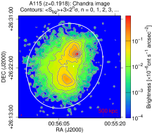
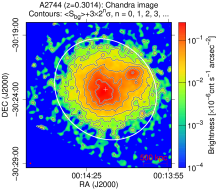
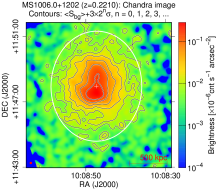
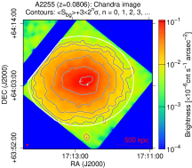
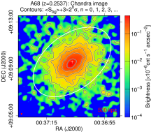
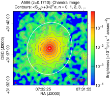
Figure 2: Example images for 6 galaxy clusters, and images for all clusters are available on the web page http://zmtt.bao.ac.cn/galaxy_clusters/dyXimages/. Cluster name, redshift and contour levels are written on the top of each panel. Surface brightness is logarithmically indicated as the color bar on the right of each panel. We select a clean region around every clusters to calculate the mean brightness $\langle S_{bg}\rangle$, and its fluctuations $\sigma$. The white cross stands for the center $(x_{0},y_{0})$ of the best fitted model. The adaptive dynamical parameters are calculated within the white ellipse, which also defines the actual region for the morphology parameters of clusters. The red circle in the bottom-left corner of each panel indicates the smooth scale generally with a diameter of 30 kpc. The scale of 500 kpc is plotted on the bottom-right corner to indicate the physical scale of clusters, which is also the radius size used to calculate the concentration index, the centroid shift and the power ratio.

In total, we have a sample of 964 galaxy clusters with good Chandra X-ray image data (see Table 1), which mostly have a lower redshift less than 0.5 (see Figure 1) but some high redshift clusters up to $z\sim 1.5$ (e.g., SPT-CL J2040-4451) do come out. The estimated masses of some clusters (e.g., Piffaretti et al., 2011) are in the range from $10^{13}M_{\odot}$ (e.g., MCXC J1242.8+0241) to $2.0\times 10^{15}M_{\odot}$ (e.g., MACS J0417.5-1154).

Table 1: Dynamical parameters for 964 clusters of galaxies (see http://zmtt.bao.ac.cn/galaxy_clusters/dyXimages/ for the full table).

Name	obsID	RA	DEC	$z$	${\rm log}_{10}(c)$	${\rm log}_{10}(\omega)$	${\rm log}_{10}(P_{3}/P_{0})$	$\kappa$	${\rm log}_{10}(\alpha)$	$\delta$
(1)	(2)	(3)	(4)	(5)	(6)	(7)	(8)	(9)	(10)	(11)
SPT-CLJ0000-5748	18238	0.25000	-57.80695	0.7020	-0.29$\pm$0.01	-3.50$\pm$0.01	-8.15$\pm$0.22	0.80	-1.19$\pm$0.01	-0.02$\pm$0.01
SPT-CLJ0001-5440	19761	0.40583	-54.66972	0.7300	-0.50$\pm$0.01	-1.53$\pm$0.01	-3.99$\pm$0.05	1.40	-0.34$\pm$0.01	1.00$\pm$0.01
A2717	6974	0.80042	-35.92722	0.0490	-0.30$\pm$0.01	-2.91$\pm$0.01	-7.58$\pm$0.01	1.40	-1.94$\pm$0.01	-0.09$\pm$0.01
Z15	12251	1.58453	10.86429	0.1663	-0.53$\pm$0.01	-2.51$\pm$0.01	-7.14$\pm$0.02	1.15	-1.76$\pm$0.01	-0.15$\pm$0.01
ACT-CLJ0008.1+0201	19586	2.04333	2.02000	0.3651	-0.67$\pm$0.01	-2.44$\pm$0.01	-6.46$\pm$0.07	2.00	-0.88$\pm$0.01	1.07$\pm$0.01
WHLJ001037.1+112957	20514	2.65464	11.49916	0.1042	-0.62$\pm$0.01	-3.16$\pm$0.01	-4.82$\pm$0.01	1.91	-0.70$\pm$0.01	1.13$\pm$0.01
A2734	5797	2.83625	-28.85500	0.0625	-0.60$\pm$0.01	-2.53$\pm$0.01	-6.80$\pm$0.01	1.49	-1.50$\pm$0.01	0.28$\pm$0.01
ZwCl0008.8+5215	19916	2.85667	52.52806	0.1040	-1.07$\pm$0.01	-1.04$\pm$0.01	-5.42$\pm$0.01	1.44	-0.81$\pm$0.01	0.71$\pm$0.01
MACS-J0011.7-1523	6105	2.92875	-15.38944	0.3780	-0.41$\pm$0.01	-3.05$\pm$0.01	-7.11$\pm$0.05	0.96	-1.72$\pm$0.01	-0.26$\pm$0.01
A7	15157	2.93861	32.41566	0.1026	-0.70$\pm$0.01	-2.47$\pm$0.02	-6.77$\pm$0.03	1.80	-1.63$\pm$0.01	0.42$\pm$0.01

Notes. Columns: (1) cluster name; (2) observation ID of Chandra; (3-4) right ascension and declination in J2000; (5) redshift; (6) the concentration index; (7) the centroid shift; (8) the power ratio; (9) the profile parameter; (10) the asymmetry factor; (11) the morphology index.

2.2 Image processing

The Chandra data for these clusters of galaxies are processed in the standard manner by using CIAO 4.9 (Fruscione et al., 2006) and calibration database CALDB 4.7.2. Data files of all observations are downloaded with CIAO command download_chandra_obsid, and reprocessed by chandra_repro to make sure the latest calibration products are used. To be consistent with previous works (e.g., Santos et al., 2008), the photons are filtered in 0.5-5 keV band. To remove flare events, we use the tool lc_clean to cut out data in time intervals where the photon count rate deviates from their mean value more than 20%. For few clusters with giant flares, the mean count rate of photons is not a good reference, thus time intervals for giant flares are removed manually. Point sources are detected automatically with the CIAO routine wavdetect with a proper threshold which should not be too high to miss some faint point sources, or not too low to lead a false detection of some fluctuations as being point sources. The size of point source model should not be too small to miss some relatively large member or foreground galaxies, or too large to confuse the core of relaxed clusters as point sources. We check the list of point sources very carefully and then remove the real point sources. We use the tool dmfilth to fill “holes” of subtracted point sources according to the brightness of ambient regions. Images of clusters are also exposure corrected and background subtracted accordingly. Since the pixel stands for different physical scales for different redshifts, the X-ray images of clusters are smoothed to 30 kpc by a Gaussian function, except for 4 very close clusters NGC 1395, Virgo, MCXC J1242.8+0241 and MCXC J1315.3-1623 with $z<0.01$ for which the smooth scale are set to 10 kpc. For few clusters without available redshifts, the images are smoothed to 5 arcseconds. The examples of final X-ray images are shown in Figure 2.

3 Dynamical parameters from X-ray images

In this section, we obtain three widely used dynamical parameters, i.e., the concentration index $c$, the centroid shift $\omega$, the power ratio $P_{3}/P_{0}$, and compare our results with those available in literature. Then, we define two adaptive dynamical parameters, i.e., the profile parameter $\kappa$ and the asymmetry factor $\alpha$, in the best fitted elliptical region. We combine them to make the morphology index $\delta$, which is an excellent indicator for the dynamical state of galaxy clusters.

3.1 Three widely used dynamical parameters

3.1.1 The concentration index, $c$

Relaxed clusters usually host a very luminous cool core in their center (e.g., Fabian et al., 1984; Fabian, 1994; McDonald et al., 2012), while the core of disturbed clusters generally have been destroyed by violent merger events. Santos et al. (2008) defined the concentration index as the ratio of X-ray fluxes integrated in the centroid and the whole regions of galaxy clusters to quantify their dynamical state. The concentration index $c$ is calculated in two circular regions with the core radius of 100 kpc and the outer radius of 500 kpc (e.g., Cassano et al., 2010, 2013), i.e.,

$$c=\frac{S_{100~{}\rm kpc}}{S_{500~{}\rm kpc}}=\frac{\sum\limits_{R<100\rm~{}kpc}f_{\rm obs}(x_{i},y_{i})}{\sum\limits_{R<500\rm~{}kpc}f_{\rm obs}(x_{i},y_{i})},$$ (1)

where $f_{\rm obs}(x_{i},y_{i})$ means the observed X-ray flux at pixel $(x_{i},y_{i})$. With the definition in Equation 1, we set the two radii as being 100 kpc and 500 kpc, and calculate the concentration index $c$ for clusters in our sample, as listed in Table 1. The concentration index for some low-redshift clusters (e.g., the Vigro cluster) cannot be calculated due to the size of 500 kpc is much out of the coverage of the Chandra CCD, and they are denoted as “–” in the full Table 1.

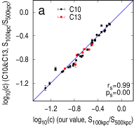
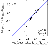
Figure 3: Comparison for the concentration indexes that we obtained with those in literatures. The solid line in panels a and b and dotted line in panel d indicate equivalent values in X and Y axes because the values in both axes are calculated with the same radii for the center and outer regions. The Spearman rank-order correlation coefficient $r_{\rm s}$ and the relevant significance $p_{\rm s}$ are labelled in the right-bottom corner of each panel. Data for the X-axis are our values and for the Y-axis are obtained from: C10=Cassano et al. (2010), C13=Cassano et al. (2013), D16=Donahue et al. (2016), A17=Andrade-Santos et al. (2017), Z17=Zhang et al. (2017) and L18=Liu et al. (2018).

Although the concentration index has been derived by a lot of authors from Chandra and/or XMM-Newton images, the radii of the central and the outer regions are chosen differently. In Figure 3, we compare our values with those calculated in literatures. Cassano et al. (2010) defined the concentration index as $c=S_{100\rm~{}kpc}/S_{500\rm~{}kpc}$ and calculated the $c$ for 32 clusters based on the Chandra images and for 7 clusters in a later paper (Cassano et al., 2013). Since we set the same core and outer radii as Cassano et al. (2010, 2013), we obtain almost the same values (see Figure 3a). Very good correlations can be found between our values of $c=S_{100\rm~{}kpc}/S_{500\rm~{}kpc}$ and those obtained by Donahue et al. (2016) in Figure 3b for 25 clusters who also defined the core radius of 100 kpc and the outer radius of 500 kpc, and in Figure 3c and Figure 3d for 19 clusters with the core radius of $0.15~{}R_{500}$ and the outer radius of $0.5~{}R_{500}$ which we also calculated. Here $R_{500}$ is the radius of a galaxy cluster within which the matter density of a cluster is 500 times of the critical density of the universe. Andrade-Santos et al. (2017) worked on a large sample of 214 clusters with the Chandra data, and calculated the concentration index with two definitions, i.e., $c=S_{40\rm~{}kpc}/S_{400\rm~{}kpc}$ and $c=S_{0.15~{}R_{500}}/S_{R_{500}}$. Again, good consistences are found between our values of $c=S_{100\rm~{}kpc}/S_{500\rm~{}kpc}$ and those in Andrade-Santos et al. (2017), see Figure 3e and Figure 3f. The outliers, i.e., A115, A2440, A3716 and RXC J1414.2+7115, in Figure 3e and Figure 3f are merging clusters with a bi-model brightness distribution (see the image of A115 in Figure 2 as an example). For these clusters we take the best-fitted center (see Section 3.2.1) located between the two subclusters similar to Cassano et al. (2010), while Andrade-Santos et al. (2017) took the X-ray peak of one subcluster as the center, which cause the value difference. There are 53 clusters in common among our sample and Zhang et al. (2017), inverse correlation appears with large scatter in Figure 3g because they define reversely as $c_{\rm L}=S_{R_{500}}/S_{0.2~{}R_{500}}$. Liu et al. (2018) calculated $c=S_{40\rm~{}kpc}/S_{400\rm~{}kpc}$ for 41 clusters from the Chandra images. We also get a good agreement between our values and results of Liu et al. (2018) for 41 clusters as shown in Figure 3h. The Spearman rank-order correlation coefficient $r_{\rm s}$, and the relevant significance $p_{\rm s}$, are marked inside each panel to show the reliability of correlations (see Press et al., 1992, p. 640). Here the small value of $p_{\rm s}$ indicates a significant correlation between the two values.

The concentration index can be calculated within the widely used, mass-related radius $R_{500}$, but there are some limitations for a large sample of clusters. First, the radius $R_{500}$ is the byproduct during the mass estimation for clusters, which (1) requires redshifts that for 53 clusters in our sample are missing, (2) needs good quality of X-ray image with sufficient photons for spectrum analysis and (3) is estimated with the assumption of spherically symmetry and virial equilibrium that is invalid for many clusters as seen in this paper. Second, the aperture with a radius of $R_{500}$ is also too large for the Chandra CCD coverage for many clusters. The median $R_{500}$ for 1,742 clusters in Piffaretti et al. (2011) is about 0.8 Mpc, the corresponding aperture exceeds 10 arcminutes when $z<0.15$ (note that the scale of the whole field of view for ACIS-I is 16.9’$\times$16.9’ and ACIS-S is 8.3’$\times$50.6’).

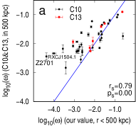
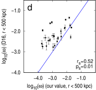
Figure 4: Comparison for the centroid shifts we calculated with those in literatures. The solid line in the panels a and d indicates equivalent values in X and Y axes if the radius is set in the same value of 500 kpc, the dotted line in panel f is also an equivalent line but for the radius of $0.5~{}R_{500}$. The correlation parameter $r_{\rm s}$ and $p_{\rm s}$ are labelled in the right-bottom corner of each panel. Data in the X-axis are our values and in the Y-axis are obtained from: C10= Cassano et al. (2010), C13=Cassano et al. (2013), W13a=Weißmann et al. (2013a), W13b=Weißmann et al. (2013b) and D16=Donahue et al. (2016).

3.1.2 The centroid shift, $\omega$

The observed X-ray image peak of merging clusters can be off from their fitted center significantly (e.g., Mohr et al., 1993; Kolokotronis et al., 2001), while the deviation is usually inconspicuous for relaxed clusters. Poole et al. (2006) defined the centroid shift $\omega$ as the standard deviation of the projected separation between the X-ray brightness peak and the model fitted center, which is computed in a series of circular aperture centered on the X-ray brightness peak from $0.05~{}R_{\rm ap}$ to $R_{\rm ap}$ in steps of $0.05~{}R_{\rm ap}$ (see also O’Hara et al., 2006), thus

$$\omega=[\frac{1}{n-1}\sum\limits_{i}(\Delta_{i}-\langle\Delta\rangle)^{2}]^{\frac{1}{2}}\times\frac{1}{R_{\rm ap}}.$$ (2)

Here $R_{\rm ap}=500~{}\rm{kpc}$ and $n=20$, $\Delta_{i}$ is the distance between the X-ray brightness peak and the fitted model center of the $i$th aperture, $\langle\Delta\rangle$ is the mean value of all $\Delta_{i}$ (e.g., Cassano et al., 2010, 2013). We calculate in this work the centroid shift for clusters in central region with radius of 500 kpc, see Equation 2 and values are listed in Table 1.

Previously, the centroid shift of clusters has been calculated by several authors with the similar formula, but for different regions. In Figure 4, the values of centroid shift $\omega$ that we obtained are compared with those calculated in literatures. Cassano et al. (2010) derived the centroid shift for 32 clusters in the aperture with a radius of 500 kpc, and 7 new clusters later in Cassano et al. (2013). Good correlation is found between our values and parameters in Cassano et al. (2010, 2013), as shown in Figure 4a. Weißmann et al. (2013a) calculated the centroid shift for 80 clusters by using the XMM-Newton images in the annulus region of 0.1–1 $R_{500}$. Weißmann et al. (2013b) worked on a larger sample of clusters in $R_{500}$ which contains 126 clusters based on Chandra and XMM-Newton data. We get good correlations, with large scatter, between our values and parameters for 57 clusters in Weißmann et al. (2013a) as shown in Figure 4b, and for 101 clusters in Weißmann et al. (2013b) in Figure 4c. Donahue et al. (2016) calculated the centroid shift for 25 clusters in 500 kpc, and for 19 clusters in 0.5 $R_{500}$ with the Chandra images. We find clear correlations between our values and those in Donahue et al. (2016), as shown in Figure 4d and Figure 4e, with large uncertainties. We also calculate the centroid shift for 19 clusters in Donahue et al. (2016) within the radius of $0.5~{}R_{500}$, and compare our values to their results in Figure 4f, and find the data are around the equivalent line with a better correlation.

In Figure 4a and 4d, the centroid shift are calculated within the same radius of 500 kpc, but our results seem to be systematically smaller than those obtained by Cassano et al. (2010, 2013) and Donahue et al. (2016), especially for relaxed clusters. This is mainly caused by the smoothed images we use. For example, Z2701 and RXC J1504.1-0248 (marked in Figure 4a) have the largest deviations to the equivalent line. The logarithmic value of the centroid shift for Z2701 is equal to -4.37 when the image is smoothed to 30 kpc, but it reduces to -3.47 when the image is smoothed to 10 kpc, and to -2.50 for unsmoothed image which matches the value of -2.44 obtained by Cassano et al. (2010) very well. The logarithm of the centroid shift for RXC J1504.1-0248 is equal to -4.00 when the image is smoothed to 30 kpc, but it is reduced to -3.31 when the image is smoothed to 10 kpc, and to -2.06 for unsmoothed image which is slightly smaller than the -2.33 obtained by Cassano et al. (2010). The smooth scale can therefore affect the value of centroid shift significantly. Considering that the pixel size stands for different physical scales for clusters with different redshifts, we suggest that the X-ray images of clusters should be smoothed to a certain physical size such as the 30 kpc we used.

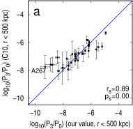
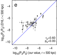
Figure 5: Comparison for the power ratios that we calculated with those in literatures. The solid line in the panels a and e indicates equivalent values in X and Y axes if the radius is set in the same value of 500 kpc, the dotted line in panel g is also an equivalent line but for the radius of $0.5~{}R_{500}$. The correlation parameter $r_{\rm s}$ and $p_{\rm s}$ are labelled in the right-bottom corner of each panel. Data in the X-axis are our values and in the Y-axis are taken from: C10=Cassano et al. (2010), W13a=Weißmann et al. (2013a), W13b=Weißmann et al. (2013b) and D16=Donahue et al. (2016).

3.1.3 Power ratio, $P_{3}/P_{0}$

Because disturbed clusters generally have more remarkable fluctuations of surface brightness than relaxed clusters, Buote & Tsai (1995) defined the power ratio as dimensionless morphological parameters from the two-dimensional multipole expansion of the projected gravitational potential of clusters within $R_{\rm ap}=500\rm kpc$. The moments, $P_{m}$, are defined as follows:

$$P_{0}=[a_{0}\ln(R_{\rm ap})]^{2},$$ (3)

$$P_{m}=\frac{1}{2m^{2}R_{\rm ap}^{2m}}(a_{m}^{2}+b_{m}^{2}).$$ (4)

The moments $a_{m}$ and $b_{m}$ are calculated using

$$a_{m}=\int_{r\leq R_{\rm ap}}f_{\rm obs}(x_{i},y_{i})(r)^{m}\cos(m\theta)dx_{i}dy_{i},$$ (5)

and

$$b_{m}=\int_{r\leq R_{\rm ap}}f_{\rm obs}(x_{i},y_{i})(r)^{m}\sin(m\theta)dx_{i}dy_{i},$$ (6)

where $f_{\rm obs}(x_{i},y_{i})$ and $\theta$ have the same meaning as before. $P_{3}/P_{0}$ is the power ratio, which was found to be related to substructures (e.g., Bauer et al., 2005; Böhringer et al., 2010; Cassano et al., 2010; Lovisari et al., 2017; Cialone et al., 2018). Following the custom, we take the radius at 500 kpc to calculate the power ratio, see Equation 3-6, and list the results in Table 1.

The values of power ratio that we obtained are compared with those calculated in literatures in Figure 5. Our values show good consistence to those obtained by Cassano et al. (2010) for 32 clusters in central region with radius of 500 kpc, as shown in Figure 5a. Weißmann et al. (2013a) worked out power ratios for 80 clusters by using the XMM-Newton images in $R_{500}$, and also defined $(P_{3}/P_{0})_{\rm max}$ as the maximum value in different annuluses along the radial direction (see details in Weißmann et al., 2013a). We get 57 clusters in common and find good correlations between our results and those in Weißmann et al. (2013a), see Figure 5b for $P_{3}/P_{0}$ and Figure 5c for $(P_{3}/P_{0})_{\rm max}$. By combining the XMM-Newton and Chandra data, Weißmann et al. (2013b) calculated power ratios for 126 galaxy clusters in $R_{500}$. The Figure 5d shows a clear correlation between values calculated by us and those in Weißmann et al. (2013b) for 101 clusters in common. Donahue et al. (2016) derived power ratios for 25 clusters in 500 kpc and 19 clusters in $0.5~{}R_{500}$ from the Chandra images. Good consistencies can be found between our results and values for clusters from Donahue et al. (2016) in Figure 5e and Figure 5f. In Figure 5g, we show the correlation between power ratios in $0.5~{}R_{500}$ calculated by us and those obtained by Donahue et al. (2016).

In Figure 5a, 5e and 5g, the power ratios in X-axis and Y-axis are calculated in the same radius, so that the values obtained by us match well with those calculated by Cassano et al. (2010) and Donahue et al. (2016) around the equivalent line. However, we get slightly smaller power ratios for relaxed clusters than those in Cassano et al. (2010) and Donahue et al. (2016) because we use the smoothed images. For example, the logarithm of the power ratio of A267, which has the largest deviation and labelled in Figure 5a, is equal to -9.28$\pm$0.34 when the image is smoothed to 30 kpc, and it is reduced to -7.24$\pm$0.48 when we use the unsmoothed image which matches very well with the value of 7.75$\pm$0.83 obtained by Cassano et al. (2010).

3.2 A new morphological parameter for estimating the dynamical state

In this subsection, we introduce and calculate a new morphological parameter for estimating the dynamical state of galaxy cluster.

As seen in section 3.1, the concentration index $c$, the centroid shift $\omega$ and the power ratio $P_{3}/P_{0}$, which have been widely used, are mostly calculated in the region of a fixed radius of 500 kpc or $R_{500}$ in recent papers. Obviously the fixed size to 500 kpc is not the best choice because clusters have various sizes. Second, these three dynamical parameters are defined and calculated in a circular region but the morphologies for most clusters are elliptical or even irregular. Third, the redshift information is needed but may not be available to define the 500 kpc or $R_{500}$, especially for clusters identified in X-ray band or through SZ effect. For clusters containing two or more subclusters, the central region for calculating the dynamical parameters can only focus on the main subcluster, which is not a proper indicator for the dynamical state of the whole cluster (such as A115 in Figure 2).

The dynamical state of clusters should be derived in regions adaptive to their size. The concerned region should be more reasonably taken as being an elliptical region rather than a circular region. The image edge of clusters in practice often is shown by the $\langle S_{bg}\rangle+3\sigma$ contours, as the white ellipse in Figure 2. The dynamical state of clusters should be independent to the exposure time of X-ray images. In the following, we use two parameters to describe the global morphological properties of clusters which are less influenced by the quality of X-ray images. We carry a few steps toward the goal as following.

3.2.1 Model fitting for the cluster shape

To describe the global morphology of a galaxy cluster, we fit the X-ray surface brightness distribution with an elliptical 2-dimensional $\beta$-model (Cavaliere & Fusco-Femiano, 1976; Guennou et al., 2014):

$$f_{\rm mod}(x_{i},y_{i})=f_{\rm mod}(r)=A(1+(\frac{r}{r_{0}})^{2})^{-\beta}+C,$$ (7)

where

$$r(x_{i},y_{i})=\frac{\sqrt{x^{2}(1-\epsilon)^{2}+y^{2}}}{1-\epsilon},$$ (8)

and

$$\begin{split}x=(x_{i}-x_{0})\cos\theta+(y_{i}-y_{0})\sin\theta,\\ y=(y_{i}-y_{0})\cos\theta-(x_{i}-x_{0})\sin\theta.\end{split}$$ (9)

Here $(x_{0},y_{0})$ are the coordinates of the center of the model, $A$ is the model amplitude, $r_{0}$ means the core radius, $\beta$ is the power law index, and $C$ is a constant adjusting the count number for the average background. $\epsilon$ is the ellipticity of cluster, $\theta$ is the position angle of cluster, defined as the direction of major axis from north to east. All these model parameters can be determined by the least $\chi^{2}$ fitting.

We fitted the model to the X-ray image of 964 clusters of galaxies, and obtained the model parameters which define the shape of galaxy clusters. Among them, the most important is the index $\beta$, which define steepness of the brightness profile. Others are not very important for the dynamical state. After the model fitting, the residual maps show more clearly the disturbed gas distribution. We have tried some quantitative description of such disturbed state, and found that the key factor is the asymmetry factor $\alpha$ (described below), which in fact can be calculated free from the model fitting, though the center has to be determined by the model-fitting.

3.2.2 Two key morphology parameters derived from Chandra X-ray images

By looking at hundreds of X-ray images of clusters and the residual images, we find that relaxed clusters generally have steeper radial distribution of brightness than disturbed ones. Further more, relaxed clusters generally have roundish morphologies while merging clusters could show more elongated shapes. Thus, we define a new profile parameter $\kappa$ for the brightness distribution as being

$$\kappa=\frac{1+\epsilon}{\beta}.$$ (10)

Here, $\beta$ and $\epsilon$ are the power law index and the ellipticity for the fitted $\beta$-model.

Disturbed clusters usually are more significantly asymmetric than relaxed ones (e.g., West et al., 1988; Okabe et al., 2010; Zhang et al., 2010; Rasia et al., 2013; Wen & Han, 2013). Here we use the asymmetry factor $\alpha$ to reveal the dynamical state of galaxy clusters, which is defined as being

$$\alpha=\frac{\sum\limits_{x_{i},y_{i}}{[f_{\rm obs}(x_{i},y_{i})-f_{\rm obs}(x_{i}^{\prime},y_{i}^{\prime})]^{2}}}{\sum\limits_{x_{i},y_{i}}{f^{2}_{\rm obs}(x_{i},y_{i})}}\times 100\;\%,$$ (11)

where $f_{\rm obs}(x_{i}^{\prime},y_{i}^{\prime})$ stands for observed flux at the symmetry pixel of $(x_{i},y_{i})$ with respect to the cluster center $(x_{0},y_{0})$.

Table 2: Dynamical parameters for 125 clusters with known dynamical states from literatures (see http://zmtt.bao.ac.cn/galaxy_clusters/dyXimages/ for the full table).

Name	ObsID	R.A.	Dec.	$z$	${\rm log}_{10}(c)$	${\rm log_{10}}(\omega)$	${\rm log_{10}}(P_{3}/P_{0})$	$\kappa$	${\rm log}_{10}(\alpha)$	$\delta$	comment
(1)	(2)	(3)	(4)	(5)	(6)	(7)	(8)	(9)	(10)	(11)	(12)
MACS0011.7-1523	6105	2.9288	-15.3894	0.3780	-0.41$\pm$0.01	-3.05$\pm$0.01	-7.11$\pm$0.05	0.96	-1.72$\pm$0.01	-0.26$\pm$0.01	R, 1
A2744	8477	3.5883	-30.3969	0.3014	-0.99$\pm$0.01	-1.68$\pm$0.01	-6.11$\pm$0.03	1.57	-0.58$\pm$0.01	0.96$\pm$0.01	D, 4
CL0016+1626	520	4.6408	16.4381	0.5410	-0.80$\pm$0.01	-2.39$\pm$0.04	-6.88$\pm$0.10	1.53	-1.25$\pm$0.01	0.48$\pm$0.01	D, 3
MACSJ0025.4-1222	10413	6.3725	-12.3769	0.5843	-0.82$\pm$0.01	-2.02$\pm$0.02	-6.34$\pm$0.05	1.97	-1.26$\pm$0.01	0.79$\pm$0.01	D, 4
RXJ0027.6+2616*	14012	6.9575	26.2739	0.3668	-0.74$\pm$0.01	-2.17$\pm$0.01	-6.66$\pm$0.04	1.74	-1.11$\pm$0.01	0.73$\pm$0.01	D, 3
MACSJ0035.4-2015	3262	8.8608	-20.2628	0.3640	-0.61$\pm$0.01	-2.14$\pm$0.01	-7.43$\pm$0.08	1.13	-1.75$\pm$0.01	-0.16$\pm$0.01	D, 3
A68*	3250	9.2785	9.1567	0.2537	-0.69$\pm$0.01	-1.81$\pm$0.01	-6.61$\pm$0.02	1.57	-1.37$\pm$0.01	0.42$\pm$0.01	D, 2
A2813	9409	10.8517	-20.6214	0.2924	-0.69$\pm$0.01	-1.93$\pm$0.01	-7.43$\pm$0.11	1.34	-1.62$\pm$0.01	0.09$\pm$0.01	D, 4
Z348	10465	16.7105	1.0697	0.2514	-0.19$\pm$0.01	-3.84$\pm$0.01	-7.51$\pm$0.02	0.65	-1.50$\pm$0.01	-0.34$\pm$0.01	R, 1
MACSJ0111.5+0855	3256	17.8813	8.9275	0.2630	-0.26$\pm$0.02	-3.49$\pm$0.05	-6.13$\pm$0.04	0.72	-1.62$\pm$0.01	-0.37$\pm$0.01	D, 2

Notes: Columns: (1) cluster name; (2) observation ID of Chandra (3-4) right ascension and declination (J2000); (5) redshift; (6) the concentration index; (7) the centroid shift; (8) the power ratio; (9) the profile parameter; (10) the asymetry factor; (11) the morphology index; (12) Comments on dynamical state of clusters: “R/D” means relaxed or disturbed clusters, the number are dynamical flag classified by Mann & Ebeling (2012). Clusters marked with “*” are selected from the BCS and eBCS catalogue (Ebeling et al., 1998, 2000) with the same selection criteria used by Mann & Ebeling (2012), and dynamically categorized by us with the standard in Mann & Ebeling (2012).

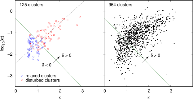
Figure 6: Left panel: Distribution for a test sample of 125 clusters in the $\kappa-\alpha$ space. The relaxed clusters are presented as circles while disturbed clusters as crosses. The dash line stands for the best fitted line for all sources in the test sample, the green solid line is the adopted boundary that separates relaxed and disturbed clusters with highest success rate. Right panel: Similar to the left panel but for 964 clusters.

Because the dynamical state cannot be represented with a single parameter and an easy threshold (see Figure 6), the combination of the profile parameter $\kappa$ and the asymmetry factor $\alpha$ can indicate the dynamical state of galaxy clusters more properly. Here we define the morphology index $\delta$ as being:

$$\delta=A\kappa+B\alpha+C.$$ (12)

To find the appropriate values of the coefficients $A$, $B$ and $C$, we take a test sample of 125 clusters with known dynamical states qualitatively classified as relaxed or disturbed by Mann & Ebeling (2012) who built a statistically complete sample from their MAssive Cluster Survey (MACS: Ebeling et al., 2001; Ebeling et al., 2007, 2010) and the Brightest Cluster Sample (BCS & eBCS: Ebeling et al., 1998, 2000) based on data of the ROSAT All-sky Survey (RASS: Truemper, 1993), with a flux larger than $1\times 10^{-12}\rm erg~{}s^{-1}cm^{-2}$ in 0.1-2.4 keV and a luminosity $L_{\rm RASS}>5\times 10^{44}\rm erg~{}s^{-1}$. They collected 129 clusters and got X-ray and optical images for 108 clusters of them, and dynamically classified these clusters into 4 groups. We directly take the dynamical information of the 108 clusters from Mann & Ebeling (2012) and define clusters in group 1 as relaxed clusters and those in group 2-4 as disturbed clusters. In addition, we take 17 extra clusters from the BCS and eBCS sample (Ebeling et al., 1998, 2000) that satisfy $f_{\rm RASS}>1\times 10^{-12}\rm erg~{}s^{-1}cm^{-2}$ and $L_{\rm RASS}>5\times 10^{44}\rm erg~{}s^{-1}$ and have been observed by Chandra later, and dynamically classify them with the same standard in Mann & Ebeling (2012). In total, we have 125 clusters with known dynamical state as listed in Table 2. This test sample is X-ray flux complete and volume complete to $z\sim 0.4$ (Mann & Ebeling, 2012).

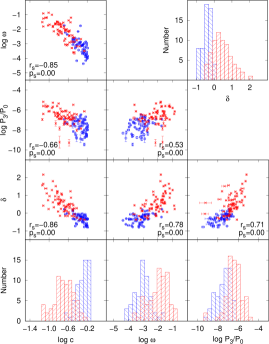
Figure 7: Left panel: One-dimensional histogram distributions and two-dimensional correlations of four kinds of dynamical proxies for 125 clusters with known dynamical states from literatures. Crosses and red histograms indicate disturbed clusters, while circles and blue histograms stand for relaxed clusters. The Spearman rank-order correlation coefficient $r_{s}$ and the relevant significance level of the correlation $p_{s}$ are labelled in each panel. A small value of $p_{s}$ indicates a significant correlation ($r_{s}$>0) or anti-correlation ($r_{s}$<0). Right panel: Similar to the left panel but for the sample of 964 clusters.

The $\kappa-\alpha$ distribution for these 125 clusters are plotted in the left panel of Figure 6. Relaxed clusters are separated from disturbed ones. First, in the $\kappa-\alpha$ space we find the best-fitted line as

$$\rm{log_{10}}(\alpha)=0.94\kappa-2.43.$$ (13)

The line of demarcation has the form of

$${\rm log_{10}}\alpha=A_{1}\kappa+B_{1},$$ (14)

which is perpendicular to the best-fitted line with $A_{1}=-1/0.94=-1.07$ and $B_{1}=-0.31$, and has the highest success rate to discriminate the relaxed and disturbed clusters. For the test sample the success rate is 115/125=88%. The morphology index $\delta$ of galaxy clusters is therefore defined as the distance to the best demarcation line in $\kappa-\alpha$ space, that is

$$\delta =0.68\rm{log_{10}}(\alpha)+0.73\kappa+0.21,$$ (15)

which can quantitatively indicate the dynamical state of galaxy clusters just from the X-ray image without the redshift information. We calculate the two parameters $\kappa$ and $\alpha$ and hence the morphology index $\delta$ for all 964 clusters, as listed in Table 1.

4 Comparison and applications of the dynamical parameters

Figure 8: Correlations between the X-ray morphology index, $\delta$, which we obtained in this paper and optical dynamical parameter, $\Gamma$, obtained by Wen & Han (2013) for 190 clusters. The Spearman rank-order correlation coefficient $r_{s}$ and the correlation significance $p_{s}$ are marked in the bottom left corner.

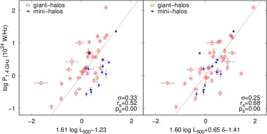
Figure 9: Applications of the morphology index $\delta$ to the scaling relations for 35 clusters with giant-halos (open circles) and 12 clusters with mini-halos (solid points). The correlation is enhanced and the scatter is reduced when the dynamical parameter $\delta$ is involved (right panel) compared to the case without involvement (left panel). The dashed line stands for the best fitted line. The intrinsic scatter $\sigma$, the Spearman rank-order correlation coefficient $r_{s}$ and the correlation significance $p_{s}$ are marked in the bottom right corner.

4.1 Comparison for the four dynamical parameters

Here we discuss the correlations among the four X-ray dynamical parameters, the concentration index, the centroid shift, the power ratio and the morphology index. To reflect the goodness of these parameters more clearly, the test sample and the whole sample of clusters are plotted and examined separately in Figure 7.

The left panels of Figure 7 show that relaxed (blue) and disturbed (red) clusters are separated in four parameters, indicating that these four parameters are sensitive diagnostics for dynamical state. However, as shown in the histograms they all are continuously distributed without a clear boundary for the two states, which is reasonable in practice. If one has to set a criterion to separate them and get the fraction of disturbed clusters, that is 48.8% if the criterion is taken as $\delta>0$, close to the value of $\sim$50% obtained by previous works based on X-ray data (Bauer et al., 2005; Chen et al., 2007; Hudson et al., 2010). In 2D parameter diagrams, clear correlations are shown between each pair of two dynamical proxies, though some of them have large scatter. The small $p_{s}$ in each panel means the correlations are significant. In the right panels, these dynamical parameters for the whole sample of 964 clusters are found to be well correlated, and also distributed continuously from very disturbed state to the relaxed state with a peak in between. Strongest correlations appear between ${\rm log}_{10}(c)$, $\delta$ and ${\rm log}_{10}(\omega)$, which implies that the three parameters are similarly sensitive to the dynamical state.

4.2 Correlation between the morphology index derived from X-ray image and the relaxation factor derived from the optical data

Based on the projected distribution of member galaxies, Wen & Han (2013) derived dynamical parameters for 2092 rich clusters. The optical image of clusters is smoothed to 20 kpc with a Gaussian kernel and weighted by luminosities of member galaxies. They got the relaxation factor $\Gamma$ by combining the asymmetry factor, the ridge flatness and the normalized deviation based on a test cluster sample with known dynamical states from literatures. We get 190 clusters by cross matching the optical catalogue in Wen & Han (2013) with our X-ray sample. The Figure 8 shows the distribution of the optical relaxation factor $\Gamma$ and the morphology index $\delta$. It is clear that relaxed clusters are both well recognized in the view of optical and X-ray dynamical parameters as the data are concentrated in the upper-left corner. However, parameters are very scattered for disturbed clusters, which means that both hot gas and member galaxies can be very disordered but are not necessary to move or distribute coincidentally.

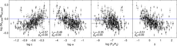
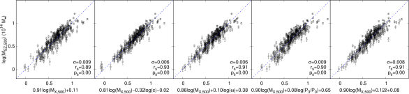
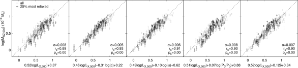
Figure 10: Top panels: Relations between dynamical parameters and ratio of mass estimated from X-ray and SZ-effect data for 316 clusters. The solid line is for the equality of the two estimated masses. Middle panels: Influence of dynamical parameters on the $M_{\rm X,500}-M_{\rm SZ,500}$ scaling relations for 316 clusters. The dashed line is the best fitted line, and the intrinsic scatter $\sigma$, the Spearman rank-order correlation coefficient $r_{s}$ and the correlation significance $p_{s}$ are marked in the bottom right corner. Bottom panels: Similar to the middle panels but for the $L_{\rm X,500}-M_{\rm SZ,500}$ relation. The 25% most relaxed clusters ($\delta<-0.15$) are denoted as black circles.

4.3 The scaling relations and the fundamental plane for radio giant-halos and mini-halos in clusters

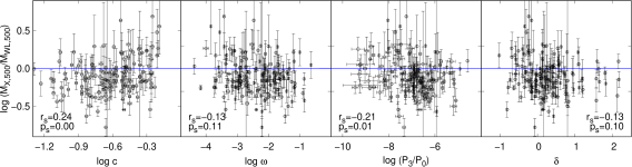
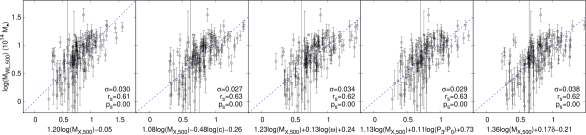
Figure 11: Similar to Figure 10 but for masses estimated through weak lensing analyses.

Large scale diffuse radio sources in clusters are associated with ICM rather than member galaxies, which can be classified into giant-halos, relics and mini-halos (see Feretti et al., 2012, as an observational review). It has been widely believed that the formation of diffuse radio sources are related to merging process of their host clusters. Giant-halos and relics are usually discovered in disturbed clusters, while mini-halos are detected around the cool core of relaxed clusters. Giant-halos and mini-halos may related to the (re-)acceleration process by turbulence in the ICM, while relics are related to the shock resulted by major merger (see Brunetti & Jones, 2014, for detail). The scaling relation has been established between radio power of giant-halos and mini-halos and the mass or mass proxies of the host clusters (e.g., Liang et al., 2000; Brunetti et al., 2009; Cassano et al., 2013; Yuan et al., 2015).

We collected the radio powers $P_{1.4~{}\rm GHz}$ in $10^{24}\rm~{}W~{}Hz^{-1}$, the X-ray luminosities $L_{500}$ within $R_{500}$ in $10^{44}\rm~{}erg~{}s^{-1}$ from Yuan et al. (2015, see the references therein). Now we check if the morphology index $\delta$ can reduce the scatter of data and enhance the correlation for the scaling relation. In the left panel of Figure 9, the radio power of giant-halos (red open circles) for 35 clusters and mini-halos (blue solid points) for 12 clusters are plotted against X-ray luminosity of host clusters. The mini-halos have statistically less radio power than giant-halos but follow the same scaling relation with the X-ray luminosity. We fit all these data with weight of data errors, see the Appendix in Yuan et al. (2015). The scaling relation has a Spearman rank-order correlation coefficient $r_{s}=0.52$. In the right panel, the morphology index is involved and the scaling relation show a larger correlation index ($r_{\rm s}=0.68$) and a reduced scatter ($\sigma=0.25$), which means that giant-halos and mini-halos follow the similar fundamental plane between the radio power, cluster mass and the morphology index.

4.4 Influence of dynamical state on mass estimation for clusters

The gravitational mass of clusters is an essential parameter for a lot of researches, which is however affected by the dynamical state if they are estimated from X-ray images. Piffaretti et al. (2011) published a meta-catalogue contains 1,743 clusters based on previous works from data of ROSAT All Sky Survey. The masses $M_{\rm X,500}$ and characteristic radius $R_{500}$ of clusters are estimated homogeneously by using X-ray data. Planck Collaboration et al. (2016) detected 1,653 clusters and estimated masses $M_{\rm SZ,500}$ from SZ-effect maps, which is insensitive to dynamical states of clusters (e.g., Motl et al., 2005). Here we use a sample of 316 clusters commonly in the catalogues in Piffaretti et al. (2011) and Planck Collaboration et al. (2016) to check the influence of dynamical state on the mass estimation for clusters.

In the top panels of Figure 10, we show the distribution of four dynamical parameters against the ratio of masses estimated from X-ray and SZ-effect data, and find a clear dependence on the concentration index $c$, the centroid shift $\omega$ and the morphology index $\delta$, though the correlation is weaker for the power ratio $P_{3}/P_{0}$. The mass estimated from the X-ray images are underestimated comparing to masses derived from SZ-effect for disturbed clusters, but apparently overestimated for relaxed clusters. The SZ-effect reflects the thermal and non-thermal components of clusters simultaneously. The underestimation of mass through X-ray data for disturbed clusters may indicate that disturbed clusters have higher fraction of energy stored as non-thermal form. In the middle rank of Figure 10, the influence of dynamical parameters is considered for the correction of the mass estimation from the X-ray images on the $M_{\rm X,500}-M_{\rm SZ,500}$ relation. The Spearman rank-order correlation coefficient increase when dynamical parameters are considered.

On the other hand, the X-ray luminosity $L_{\rm X,500}$ is widely used as a mass proxy of clusters. In the bottom panels of Figure 10, we show the $L_{\rm X,500}-M_{\rm SZ,500}$ relations for the 316 clusters. Since relaxed and disturbed clusters usually show different mass scaling relations (e.g., O’Hara et al., 2006; Lopes et al., 2006; Lopes et al., 2009; Zhao et al., 2013), we compare the 25% most relaxed clusters ($\delta<-0.15$, black circles) with the full sample. For the 2D correlation (the most left panel), the relaxed clusters are clearly offset from the best fitted line determined by the total sample. The offset is significantly reduced when the dynamical parameters included (the right four panels), which again means that there is a fundamental plane for the mass, luminosity and dynamical state for galaxy clusters. The 3D correlations have smaller intrinsic scatter and larger $r_{\rm s}$ than the 2D correlation.

For the further demonstration, we investigate the influence of dynamical state to the lensing mass of galaxy clusters which is believed to be the most reliable. Sereno (2015) compiled a catalogue which contains 485 clusters with mass ($M_{\rm WL,500}$) estimated through weak lensing analyses. We cross-match our samples with the catalogues in Sereno (2015) and Piffaretti et al. (2011), and get 151 clusters in common. In Figure 11, we do similar correlations to Figure 10 but replace $M_{\rm X,500}$ with $M_{\rm WL,500}$. In the upper panels of Figure 11, the mass ratio ($M_{\rm X,500}/M_{\rm WL,500}$) is not randomly around but mostly less than 0, which means that the X-ray mass is underestimated. In the lower panels, the correlations are enhanced with slightly larger $r_{s}$ when dynamical parameters are included.

5 Summary

The Chandra satellite has accumulated X-ray image data for $\sim$1000 clusters of galaxies, which make it feasible to work out a catalogue of dynamical parameters for a large sample of clusters.

We collected Chandra data for 964 galaxy clusters. The images for these clusters are processed following the same procedure, and smoothed by a Gaussian function with a size of 30 kpc (or 5 arcseconds for few clusters with no redshift available). Three widely used dynamical parameters, i.e., the concentration index $c$, the centroid shift $\omega$ and the power ratio $P_{3}/P_{0}$, are calculated from the X-ray images in a circular region with a radius of 500 kpc. Our results are consistent with the values available in literatures. We also derive two adaptive parameters, the profile parameter $\kappa$ and the asymmetry factor $\alpha$ in the best fitted elliptical region, and define the morphology index $\delta$, which can be excellent indicator for dynamical state. Finally, we calculate the profile parameter $\kappa$, the asymmetry parameter $\alpha$ and the morphology index $\delta$ for 964 clusters (see Table 1).

The four dynamical parameters are well correlated, and can separate relaxed clusters from disturbed ones. But they are distributed continuously from the most disturbed status to the relaxed. The morphology index we derived from the X-ray images and optical relaxation factor is also significant correlated.

By involving the dynamical parameters, we find that clusters with diffuse radio giant-halos and mini-halos follow the same fundamental plane between radio power, cluster mass and morphology index. Mass estimation for cluster of galaxies if derived from X-ray data is affected by their dynamical states.

Data availability

The data underlying this article, the X-ray images for 964 clusters, and also the code for calculations are available on the web-page http://zmtt.bao.ac.cn/galaxy_clusters/dyXimages/.

References

- Abell et al. (1989) Abell G. O., Corwin Jr. H. G., Olowin R. P., 1989, ApJS, 70, 1
- Aguerri & Sánchez-Janssen (2010) Aguerri J. A. L., Sánchez-Janssen R., 2010, A&A, 521, A28
- Andrade-Santos et al. (2017) Andrade-Santos F., et al., 2017, ApJ, 843, 76
- Barrena et al. (2002) Barrena R., Biviano A., Ramella M., Falco E. E., Seitz S., 2002, A&A, 386, 816
- Bartalucci et al. (2019) Bartalucci I., Arnaud M., Pratt G. W., Démoclès J., Lovisari L., 2019, A&A, 628, A86
- Bauer et al. (2005) Bauer F. E., Fabian A. C., Sanders J. S., Allen S. W., Johnstone R. M., 2005, MNRAS, 359, 1481
- Böhringer et al. (2010) Böhringer H., et al., 2010, A&A, 514, A32
- Brunetti & Jones (2014) Brunetti G., Jones T. W., 2014, International Journal of Modern Physics D, 23, 1430007
- Brunetti et al. (2009) Brunetti G., Cassano R., Dolag K., Setti G., 2009, A&A, 507, 661
- Buote & Tsai (1995) Buote D. A., Tsai J. C., 1995, ApJ, 452, 522
- Buote & Tsai (1996) Buote D. A., Tsai J. C., 1996, ApJ, 458, 27
- Cassano et al. (2010) Cassano R., Ettori S., Giacintucci S., Brunetti G., Markevitch M., Venturi T., Gitti M., 2010, ApJ, 721, L82
- Cassano et al. (2013) Cassano R., et al., 2013, ApJ, 777, 141
- Cavaliere & Fusco-Femiano (1976) Cavaliere A., Fusco-Femiano R., 1976, A&A, 49, 137
- Chen et al. (2007) Chen Y., Reiprich T. H., Böhringer H., Ikebe Y., Zhang Y.-Y., 2007, A&A, 466, 805
- Chiang et al. (2013) Chiang Y.-K., Overzier R., Gebhardt K., 2013, ApJ, 779, 127
- Chon et al. (2012) Chon G., Böhringer H., Smith G. P., 2012, A&A, 548, A59
- Cialone et al. (2018) Cialone G., De Petris M., Sembolini F., Yepes G., Baldi A. S., Rasia E., 2018, MNRAS, 477, 139
- Colless & Dunn (1996) Colless M., Dunn A. M., 1996, ApJ, 458, 435
- Cuciti et al. (2015) Cuciti V., Cassano R., Brunetti G., Dallacasa D., Kale R., Ettori S., Venturi T., 2015, A&A, 580, A97
- Donahue et al. (2016) Donahue M., et al., 2016, ApJ, 819, 36
- Dressler & Shectman (1988) Dressler A., Shectman S. A., 1988, AJ, 95, 985
- Dupke & Bregman (2006) Dupke R. A., Bregman J. N., 2006, ApJ, 639, 781
- Ebeling et al. (1998) Ebeling H., Edge A. C., Bohringer H., Allen S. W., Crawford C. S., Fabian A. C., Voges W., Huchra J. P., 1998, MNRAS, 301, 881
- Ebeling et al. (2000) Ebeling H., Edge A. C., Allen S. W., Crawford C. S., Fabian A. C., Huchra J. P., 2000, MNRAS, 318, 333
- Ebeling et al. (2001) Ebeling H., Edge A. C., Henry J. P., 2001, ApJ, 553, 668
- Ebeling et al. (2007) Ebeling H., Barrett E., Donovan D., Ma C. J., Edge A. C., van Speybroeck L., 2007, ApJ, 661, L33
- Ebeling et al. (2010) Ebeling H., Edge A. C., Mantz A., Barrett E., Henry J. P., Ma C. J., van Speybroeck L., 2010, MNRAS, 407, 83
- Einasto et al. (2010) Einasto M., et al., 2010, A&A, 522, A92
- Einasto et al. (2012) Einasto M., et al., 2012, A&A, 540, A123
- Fabian (1994) Fabian A. C., 1994, ARA&A, 32, 277
- Fabian et al. (1984) Fabian A. C., Nulsen P. E. J., Canizares C. R., 1984, Nature, 310, 733
- Feretti et al. (2012) Feretti L., Giovannini G., Govoni F., Murgia M., 2012, A&ARv, 20, 54
- Flin & Krywult (2006) Flin P., Krywult J., 2006, A&A, 450, 9
- Fruscione et al. (2006) Fruscione A., et al., 2006, in Society of Photo-Optical Instrumentation Engineers (SPIE) Conference Series. p. 62701V, doi:10.1117/12.671760
- Geller & Beers (1982) Geller M. J., Beers T. C., 1982, PASP, 94, 421
- Guennou et al. (2014) Guennou L., et al., 2014, A&A, 561, A112
- Halliday et al. (2004) Halliday C., et al., 2004, A&A, 427, 397
- Hou et al. (2009) Hou A., Parker L. C., Harris W. E., Wilman D. J., 2009, ApJ, 702, 1199
- Hudson et al. (2010) Hudson D. S., Mittal R., Reiprich T. H., Nulsen P. E. J., Andernach H., Sarazin C. L., 2010, A&A, 513, A37
- Kale et al. (2015) Kale R., Venturi T., Cassano R., Giacintucci S., Bardelli S., Dallacasa D., Zucca E., 2015, A&A, 581, A23
- Klein et al. (2019) Klein M., et al., 2019, Monthly Notices of the Royal Astronomical Society, 488, 739
- Kolokotronis et al. (2001) Kolokotronis V., Basilakos S., Plionis M., Georgantopoulos I., 2001, MNRAS, 320, 49
- Liang et al. (2000) Liang H., Hunstead R. W., Birkinshaw M., Andreani P., 2000, ApJ, 544, 686
- Liu et al. (2015) Liu A., Yu H., Tozzi P., Zhu Z.-H., 2015, ApJ, 809, 27
- Liu et al. (2016) Liu A., Yu H., Tozzi P., Zhu Z.-H., 2016, ApJ, 821, 29
- Liu et al. (2018) Liu A., Tozzi P., Yu H., De Grandi S., Ettori S., 2018, MNRAS,
- Lopes et al. (2006) Lopes P. A. A., de Carvalho R. R., Capelato H. V., Gal R. R., Djorgovski S. G., Brunner R. J., Odewahn S. C., Mahabal A. A., 2006, ApJ, 648, 209
- Lopes et al. (2009) Lopes P. A. A., de Carvalho R. R., Kohl-Moreira J. L., Jones C., 2009, MNRAS, 392, 135
- Lopes et al. (2018) Lopes P. A. A., Trevisan M., Laganá T. F., Durret F., Ribeiro A. L. B., Rembold S. B., 2018, MNRAS, 478, 5473
- Lovisari et al. (2017) Lovisari L., et al., 2017, ApJ, 846, 51
- Mann & Ebeling (2012) Mann A. W., Ebeling H., 2012, MNRAS, 420, 2120
- Markevitch et al. (2002) Markevitch M., Gonzalez A. H., David L., Vikhlinin A., Murray S., Forman W., Jones C., Tucker W., 2002, ApJ, 567, L27
- Maughan et al. (2008) Maughan B. J., Jones C., Forman W., Van Speybroeck L., 2008, ApJS, 174, 117
- McDonald et al. (2012) McDonald M., et al., 2012, Nature, 488, 349
- McGee et al. (2009) McGee S. L., Balogh M. L., Bower R. G., Font A. S., McCarthy I. G., 2009, MNRAS, 400, 937
- Mohr et al. (1993) Mohr J. J., Fabricant D. G., Geller M. J., 1993, ApJ, 413, 492
- Mohr et al. (1995) Mohr J. J., Evrard A. E., Fabricant D. G., Geller M. J., 1995, ApJ, 447, 8
- Motl et al. (2005) Motl P. M., Hallman E. J., Burns J. O., Norman M. L., 2005, ApJ, 623, L63
- O’Hara et al. (2006) O’Hara T. B., Mohr J. J., Bialek J. J., Evrard A. E., 2006, ApJ, 639, 64
- Oguri (2014) Oguri M., 2014, MNRAS, 444, 147
- Okabe et al. (2010) Okabe N., Zhang Y.-Y., Finoguenov A., Takada M., Smith G. P., Umetsu K., Futamase T., 2010, ApJ, 721, 875
- Piffaretti et al. (2011) Piffaretti R., Arnaud M., Pratt G. W., Pointecouteau E., Melin J.-B., 2011, A&A, 534, A109
- Planck Collaboration et al. (2016) Planck Collaboration et al., 2016, A&A, 594, A27
- Poole et al. (2006) Poole G. B., Fardal M. A., Babul A., McCarthy I. G., Quinn T., Wadsley J., 2006, MNRAS, 373, 881
- Press & Schechter (1974) Press W. H., Schechter P., 1974, ApJ, 187, 425
- Press et al. (1992) Press W. H., Teukolsky S. A., Vetterling W. T., Flannery B. P., 1992, Numerical recipes in FORTRAN. The art of scientific computing
- Ramella et al. (2007) Ramella M., et al., 2007, A&A, 470, 39
- Rasia et al. (2013) Rasia E., Meneghetti M., Ettori S., 2013, The Astronomical Review, 8, 40
- Ribeiro et al. (2011) Ribeiro A. L. B., Lopes P. A. A., Trevisan M., 2011, MNRAS, 413, L81
- Roberts et al. (2018) Roberts I. D., Parker L. C., Hlavacek-Larrondo J., 2018, MNRAS, 475, 4704
- Rumbaugh et al. (2018) Rumbaugh N., et al., 2018, MNRAS, 478, 1403
- Rykoff et al. (2014) Rykoff E. S., et al., 2014, ApJ, 785, 104
- Santos et al. (2008) Santos J. S., Rosati P., Tozzi P., Böhringer H., Ettori S., Bignamini A., 2008, A&A, 483, 35
- Sereno (2015) Sereno M., 2015, MNRAS, 450, 3665
- Solanes et al. (1999) Solanes J. M., Salvador-Solé E., González-Casado G., 1999, A&A, 343, 733
- Truemper (1993) Truemper J., 1993, Science, 260, 1769
- Weißmann et al. (2013a) Weißmann A., Böhringer H., Šuhada R., Ameglio S., 2013a, A&A, 549, A19
- Weißmann et al. (2013b) Weißmann A., Böhringer H., Chon G., 2013b, A&A, 555, A147
- Wen & Han (2013) Wen Z. L., Han J. L., 2013, MNRAS, 436, 275
- Wen & Han (2015) Wen Z. L., Han J. L., 2015, MNRAS, 448, 2
- Wen et al. (2012) Wen Z. L., Han J. L., Liu F. S., 2012, ApJS, 199, 34
- Wen et al. (2018) Wen Z. L., Han J. L., Yang F., 2018, MNRAS, 475, 343
- West & Bothun (1990) West M. J., Bothun G. D., 1990, ApJ, 350, 36
- West et al. (1988) West M. J., Oemler Jr. A., Dekel A., 1988, ApJ, 327, 1
- Yahil & Vidal (1977) Yahil A., Vidal N. V., 1977, ApJ, 214, 347
- Yu et al. (2016) Yu H., Diaferio A., Agulli I., Aguerri J. A. L., Tozzi P., 2016, ApJ, 831, 156
- Yu et al. (2018) Yu H., Diaferio A., Serra A. L., Baldi M., 2018, ApJ, 860, 118
- Yuan et al. (2015) Yuan Z. S., Han J. L., Wen Z. L., 2015, ApJ, 813, 77
- Yuan et al. (2016) Yuan Z. S., Han J. L., Wen Z. L., 2016, MNRAS, 460, 3669
- Zenteno et al. (2020) Zenteno A., et al., 2020, MNRAS, 495, 705
- Zhang et al. (2008) Zhang Y.-Y., Finoguenov A., Böhringer H., Kneib J.-P., Smith G. P., Kneissl R., Okabe N., Dahle H., 2008, A&A, 482, 451
- Zhang et al. (2010) Zhang Y.-Y., et al., 2010, ApJ, 711, 1033
- Zhang et al. (2017) Zhang Y.-Y., et al., 2017, A&A, 599, A138
- Zhao et al. (2013) Zhao H.-H., Jia S.-M., Chen Y., Li C.-K., Song L.-M., Xie F., 2013, ApJ, 778, 124