Skyrmions in twisted van der Waals magnets

Abstract

Magnetic skyrmions in two-dimensional (2D) chiral magnets are often stabilized by a combination of Dzyaloshinskii-Moriya interaction and external magnetic field. Here, we show that skyrmions can also be stabilized in twisted moiré superlattices with Dzyaloshinskii-Moriya interaction in the absence of an external magnetic field. Our setup consists of a 2D ferromagnetic layer twisted on top of an antiferromagnetic substrate. The coupling between the ferromagnetic layer and the substrate generates an effective alternating exchange field. We find a large region of skyrmion crystal phase when the length scales of the moiré periodicity and skyrmions are compatible. Unlike chiral magnets under magnetic field, skyrmions in moiré superlattices show enhanced stability for the easy-axis (Ising) anisotropy which can be essential to realize skyrmions since most van der Waals magnets possess easy-axis anisotropy.

I Introduction

The discovery of ferromagnetism in two-dimensional (2D) monolayer CrI₃ and other 2D van der Waals (vdW) materials opened a new window for exploring low dimensional magnetism and its applications in spintronicsGibertini et al. (2019); Gong and Zhang (2019); Burch et al. (2018); Huang et al. (2017); Gong et al. (2017); Deng et al. (2018); Bonilla et al. (2018); O’Hara et al. (2018); Soriano et al. (2019). The properties of 2D materials can be controlled by external parametersCristoloveanu et al. (2019); Ye et al. (2012); Cao et al. (2018a); Huang et al. (2018); Song et al. (2019) and are highly sensitive to stacking and twisting between the layersPonomarenko et al. (2013); Dean et al. (2013); Gorbachev et al. (2014); Cao et al. (2018b, a). In particular, with the discovery of superconductivity in twisted bilayer grapheneCao et al. (2018b, a), there has been tremendous progress on exploring moiré superlattices both experimentally and theoretically Zhang et al. (2017); Moon and Koshino (2014); Chen et al. (2019a, b); Wallbank et al. (2015); Ni et al. (2015). In terms of magnetism, stacking order and twisting can significantly alter the interlayer exchange as the exchange is highly sensitive to atomic registriesChen et al. (2019c); Sivadas et al. (2018); Jiang et al. (2019); Du et al. (2016); Klein et al. (2018); Tong et al. (2018).

Magnetic skyrmions Roessler et al. (2006) are nanoscale vortex-like spin textures that were first observed in non-cetrosymmetic bulk magnetic materials such as MnSi Mühlbauer et al. (2009); Yu et al. (2010), (FeCo)Si Münzer et al. (2010) and FeGe Yu et al. (2011). Skyrmions are topological defects, and they exhibit novel transport phenomena such as topological Hall effect and topological Nerst effect Hamamoto et al. (2015); Shiomi et al. (2013). In recent years skyrmions received ample attention due to their potential for spintronics applications and memory storage devices Fert et al. (2013). In most cases, skyrmions are stabilized by interplay of Dzyaloshinskii-Moriya (DM) interaction and external magnetic fieldMühlbauer et al. (2009); Yu et al. (2010); Banerjee et al. (2014). In this article, we explore the possibility of stabilizing magnetic skyrmions in the absence of an external magnetic field in moiré superlattices. We consider a ferromagnetic (FM) monolayer on an antiferromagnetic (AFM) substrate with Néel order. Twisting the FM layer by an angle $\theta$ produces moiré patterns as shown in Fig. 1(a), (c). Ferromagnetic coupling between the substrate and the FM monolayer leads to an alternating exchange field for the moiré superlattice as shown in Fig. 1(b). Our setup is motivated from Ref. Tong et al., 2018. However unlike Ref. Tong et al., 2018 which includes dipole-dipole interaction to stabilize magnetic skyrmions, we consider DM interaction which is the primary interaction for magnetic skyrmions in chiral magnetsMühlbauer et al. (2009); Yu et al. (2010); Johnson et al. (1996); Dubowik (1996); Banerjee et al. (2013).

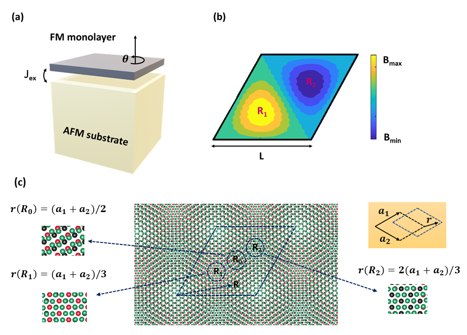
Figure 1: (a) Schematic of our setup of a FM monolayer twisted on top of an AFM substrate with Néel order. We consider honeycomb lattice for both the monolayer and the substrate. (b) Exchange field due to interlayer coupling. (c) Moiré pattern due to small twisting angle between FM monolayer (green) and top most layer of AFM substrate (red and black). Three local atomic registries $\textbf{R}_{0}$, $\textbf{R}_{1}$ and $\textbf{R}_{2}$ are zoomed which matches the atomic registries of different interlayer translations.

Our main results are summarized in Fig. 2 and 3. We show that (i) skyrmion crystal (SkX) is stabilized as a function of exchange coupling between the layers ($J_{\rm ex}$) and moiré periodicity. (ii) Even though SkX can be stabilized for a wide range of twisting angle, we find the optimal moiré periodicity to be about $L=9L_{D}$, where $L_{D}=(J/D)a$ is the intrinsic length scale for skyrmions. (iii) Unlike chiral magnets under magnetic field, we find an extended region of SkX for easy-axis anisotropy. (iv) We show that a large fraction of the topological charge $q=\frac{1}{4\pi}\int d^{2}r\widehat{\textbf{m}}.(\partial_{x}\widehat{\textbf{m}}\times\partial_{y}\widehat{\textbf{m}})$ of the magnetic skyrmions is concentrated at the edges and splits into three parts for large moiré periodicity and large easy axis anisotropy. This effect arises due to the anisotropic shape of the skyrmion.

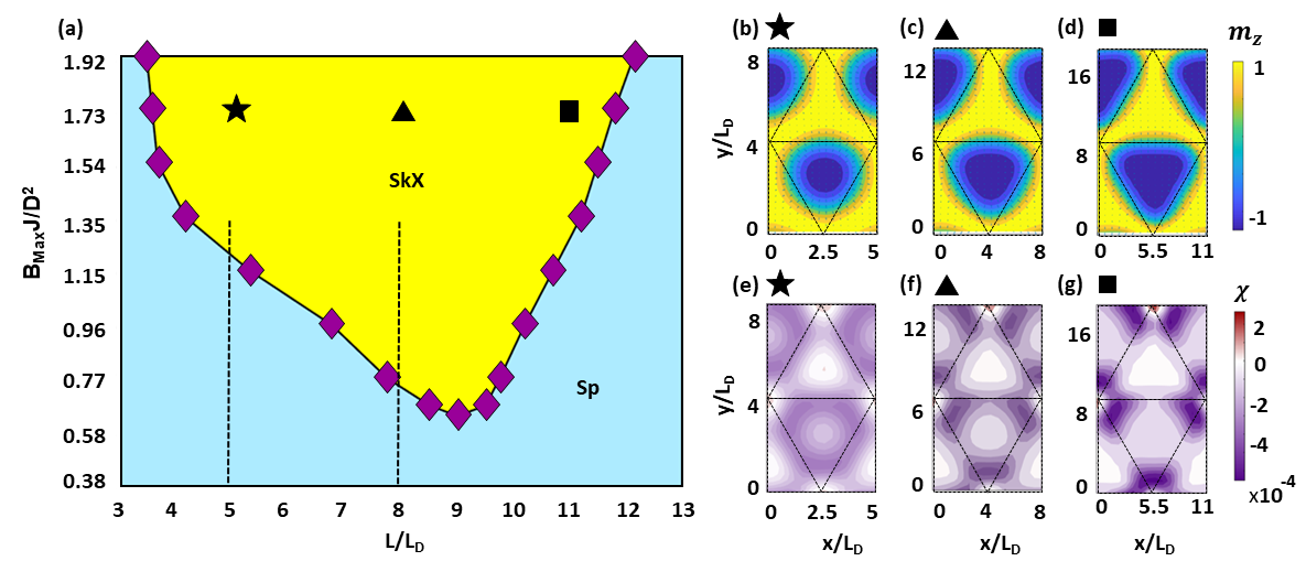
Figure 2: $A=0$ phase diagram at different moiré periods and exchange field. (a) Moiré period $L$ vs maximum interlayer exchange field $B_{Max}$ phase diagram with spiral (Sp) and skyrmion crystal (SkX) phases. Here $L_{D}=(J/D)a$, where $a$ is the lattice constant and the purple diamonds correspond to error bars. The dashed lines at $L=5L_{D}$ and $L=8L_{D}$ represent the cross section of Fig. 3(a) and Fig. 5 respectively. (b,c,d) Magnetization texture and (e,f,g) topological charge density in $1\times 2$ moiré super cells for $L/L_{D}=(5,8,11)$ and $B_{Max}J/D^{2}=1.73$ as marked by $\bigstar,\blacktriangle,\blacksquare$ symbols in (a). The colors represent out of plane component ($m_{z}$) of magnetization and topological charge density ($\chi$) in (b,c,d) and (e,f,g) respectively. The arrows show the in-plane component of magnetization in (b,c,d) and the dotted lines represent $1\times 2$ moiré super cells in (b,c,d,e,f,g).

II Model

Before we delve into the analysis of the effective magnetic Hamiltonian, we first describe our setup. As mentioned above, we follow the procedure of Ref. Tong et al., 2018 to derive the effective interlayer exchange field. We consider a FM monolayer twisted on top of an AFM substrate, both on a honeycomb lattice with the same lattice constant, $a$. For twisting angle $\theta$, the moiré period is given by $L=a/2\sin(\theta/2)$. For small angle $\theta$ and/or lattice mismatch $\delta$, $L\thickapprox a/\sqrt{\theta^{2}+\delta^{2}}$ (large period), the local atomic registries on length scale smaller than $L$ but larger than $a$ matches the atomic stacking of different interlayer translation r as shown in Fig. 1(c). Hence moiré superlattice can be described by interlayer translation vector r(R) that gives atomic registry at position R. The interlayer exchange coupling between AFM substrate and FM layer is different at different positions due to different atomic stacking of monolayer and substrate and this leads to spatially dependent exchange field B(R) as shown in Fig. 1(b). For example, at position $\textbf{R}_{1}$ the coupling aligns the spins of 2D layer (green) in positive z-direction when it sits on top of AFM sublattice with spins up (black) and the spins align in opposite direction at $\textbf{R}_{2}$ when it is on top of AFM sublattice with spins down (red). The interlayer exchange field at interlayer translation r is give by Tong et al. (2018)

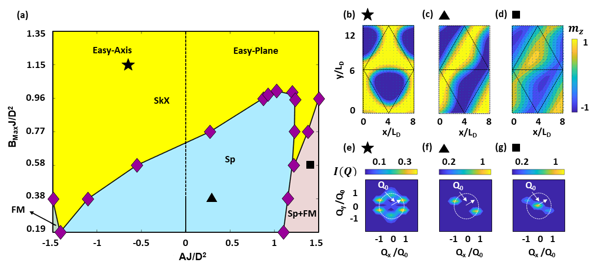
Figure 3: $L=8L_{D}$ phase diagram. (a) Anisotropy $A$ versus maximum interlayer exchange field $B_{Max}$ phase diagram with ferromagnetic (FM), spiral (Sp), skyrmion crystal (SkX) and mixed state (Sp+FM). Here $L_{D}=(J/D)a$, where $a$ is the lattice constant. (b,c,d) Magnetization texture in $1\times 2$ moiré supercells and (e,f,g) spin structure factor for ($\bigstar,\blacktriangle,\blacksquare$) symbols marked in (a). The parameters corresponding to these symbols are the following: $\bigstar$ = $\{A=-0.6D^{2}/J$, $B_{Max}=1.15D^{2}/J\}$, $\blacktriangle$ = $\{A=0.3D^{2}/J$, $B_{Max}=0.38D^{2}/J\}$ and $\blacksquare$ = $\{A=1.14D^{2}/J$, $B_{Max}=0.58D^{2}/J\}$.

$$\textbf{B}^{\tau}(\textbf{r})=\sum_{j,\tau^{\prime}}J^{\tau^{\prime}}_{ex}(\textbf{r}-\bm{\xi}_{\tau}+\textbf{R}_{j})\textbf{m}_{j,\tau^{\prime}}$$ (1)

where $J_{ex}$ is the interlayer coupling coefficient, m is the magnetic moment of top most layer of AFM substrate, $\left\{\tau,\tau^{\prime}\right\}=\left\{A,B\right\}$ represents the two in-equivalent sites in unit cell, $\bm{\xi}_{A}=0$, $\bm{\xi}_{B}=\left\{0,a\right\}$ and the summation $j$ is over the Bravais lattice. The total interlayer exchange field per unit cell is given by summing the fields of site $A$ and $B$

$$\textbf{B}(\textbf{r})=\textbf{B}^{A}(\textbf{r})+\textbf{B}^{B}(\textbf{r}).$$ (2)

This approximation holds when the interlayer coupling, $J_{ex}$ is small as compared to intralayer coupling, $J$. In general, $J_{ex}<J$ holds for vdW magnets as the interplane exchange is expected to be much smaller than intraplane exchange. We used the following coupling form that decays exponentially at long distances

$$J^{\tau^{\prime}}_{ex}(\textbf{r}-\bm{\xi}_{\tau}+\textbf{R}_{j})=J^{0}_{ex}e^{-\frac{\sqrt{(\textbf{r}-\bm{\xi}_{\tau}+\bm{\xi}_{\tau^{\prime}}+\textbf{R}_{j})^{2}+d^{2}}}{r_{0}}}$$ (3)

where $d$ is the interlayer separation and $r_{0}$ is the decay length. In our calculations we used $d=a$, $r_{0}=a$ and this leads to

$$B_{Max}\thickapprox 1.9244\times 10^{-2}J^{0}_{ex}.$$ (4)

Next we describe our model for the monolayer. We consider a magnetic model for 2D honeycomb lattice which is relevant to 2D vdW magnets such as trihallides Huang et al. (2017)

$$H = -J\sum_{{r,\mu}}{\bf S}_{r}.({\bf S}_{r+\hat{\delta}_{\mu}})-D\sum_{{r,\mu}}[\hat{d}_{\mu}.({\bf S}_{r}\times{\bf S}_{r+\hat{\delta}_{\mu}})]$$ (5)

$$-A_{c}\sum_{{r,\mu}}[({\bf S}_{r}.\hat{d}_{\mu})({\bf S}_{r+\hat{\delta}_{\mu}}.\hat{d}_{\mu})]+A_{s}\sum_{{r}}(S_{r}^{z})^{2}$$

$$-\sum_{r}{\bf B}({\bf R}_{r})\cdot{\bf S}_{r}$$

where $\vec{S}_{r}$ is local moment at site $r$ and $\hat{\delta}_{\mu}$ are the three nearest neighbors on the honeycomb lattice. $J$ is the ferromagnetic Heisenberg exchange coupling, $D$ is the DM coupling Moriya (1960b). $A_{c}$ and $A_{s}$ are the compass and single-ion anisotropies respectively. The DM vector $\hat{d}_{i}=\hat{z}\times\hat{\delta}_{i}$ is set by the symmetry and originates due to the inversion symmetry breaking on the surface. However, the microscopic mechanism for the DM interaction in insulating vdW magnets is different than metallic multilayers since the former is due to the superexchange interaction in the presence of an electric field as originally discussed by MoriyaMoriya (1960b) whereas the latter can be ascribed to asymmetric interaction paths proposed by Fert and LevyLevy and Fert (1981); Fert and Levy (1980). $\bf B(R)$ is the interlayer exchange field with the twisted substrate. To explore the phase diagram of $H$, we consider the free energy functional in the continuum $\mathscr{F}[{\bf m}]=\int d^{2}rF({\bf m})$ where ${\bf m}({\bf r})$ is the local magnetization. We set the lattice constant, $a=1$. The free energy density has the following four components

$$F({\bf m})=F_{iso}+F_{DM}+F_{aniso}+F_{moire}$$ (6)

where

$$F_{iso} = F_{0}(\textbf{m})+\frac{3}{2}(J/2)\sum_{{\alpha}}(\nabla m^{\alpha})^{2}$$ (7)

$$F_{DM} = -\frac{3}{2}D(m^{z}\partial_{x}m^{x}-m^{x}\partial_{x}m^{z})$$ (8)

$$+\frac{3}{2}D(m^{y}\partial_{y}m^{z}-m^{z}\partial_{y}m^{y})$$

$$F_{aniso} = -\frac{3}{2}A_{c}[(m^{x})^{2}+(m^{y})^{2}]+A_{s}(m^{z})^{2}$$ (9)

$$+\frac{3A_{c}}{4}[m^{y}(\partial_{x}m^{y}+\partial_{y}m^{x})$$

$$-m^{x}(\partial_{x}m^{x}-\partial_{y}m^{y})]$$

$$F_{moire} = -{\bf B(R)}\cdot{\bf m}.$$ (10)

We absorb factor $\frac{3}{2}$ in $J$, $D$ and $A_{c}$ and define the effective anisotropy $A=A_{c}+A_{s}$ which can be positive (easy plane) or negative (easy axis or Ising). The last two terms in $F_{aniso}$, given as $\sim[m^{y}(\partial_{x}m^{y}+\partial_{y}m^{x})-m^{x}(\partial_{x}m^{x}-\partial_{y}m^{y})]$ have no contribution to the free energy for systems with periodic boundary conditions since they are total derivatives. To obtain the ground state spin configuration m, we solve the coupled Landau-Lifshitz-Gilbert (LLG) equations Gilbert (2004)

$$\frac{d\textbf{m}}{dt}=-\gamma\textbf{m}\times\textbf{B}^{eff}+\alpha\textbf{m}\times\frac{d\textbf{m}}{dt},$$ (11)

where $\textbf{B}^{eff}=-\delta H/\delta\textbf{m}$, $\gamma$ is gyromagnetic ratio and $\alpha$ is Gilbert damping coefficient. We start from different initial states and compare the energies of final states to get the actual ground state. To solve LLG equations numerically we used mid point method d’Aquino et al. (2005) by discretizing the effective magnetic field $\textbf{B}^{eff}=-\delta H/\delta\textbf{m}$ on a $1\times 2$ moiré supercells. We used $L_{D}=(J/D)a=10a$ to construct the phase diagrams and the results were also verified at various points for larger values of $L_{D}$. The magnitude of the magnetization was kept constant at each grid point after each time step enforcing the hard spin constraint, $|{\bf m}|^{2}=1$ and periodic boundary conditions were imposed at the boundaries. There is unavoidable error due to solving the LLG equations on a discrete lattice. The error is small as long as the variation of the magnetization is small within neighboring sites. We checked that our results are robust as a function of increasing system.

Our method can only capture magnetic orders that are commensurate with the 1x2 moiré supercell. However, in the limit of $J_{ex}\rightarrow 0$, the ground state is a spiral with the wave vector $q\simeq D/J$ for weak anisotropyBanerjee et al. (2014) which is in general not commensurate with the moiré supercell. Therefore, our method is not suitable to explore the weak $J_{ex}$ limit. Such incommensurate phases and incommensurate to commensurate phase transitions have recently been analyzed in Ref. 47. The parameters used in this article lie outside the regime of incommensurate phasesHejazi et al. (2020), yet it is not possible to extrapolate our results to $J_{ex}\rightarrow 0$ limit due to this reason.

III Results

We start by exploring the interplay between the moiré periodicity $L$ and $B_{Max}$ as shown in Fig. 2 for $A=0$. $B_{Max}$ is the maximum value of interlayer exchange magnetic field. As shown in Fig 1(b), the moiré supercell splits into two triangles of opposite alternating effective magnetic field which is maximum at the centers and vanishingly small at the corners of the triangles. Therefore, in the limit of large $B_{Max}$, the magnetization aligns with the effective magnetic field at the center of the triangles, creating two ferromagnetic domains separated with a domain wall whose chirality is set by D. The only degree of freedom left that determines the ground state is the magnetization at the corners of the triangles which creates an effective triangular lattice. In particular, if the magnetization at the corners are ferromagnetic, the state is a skyrmion whereas a stripe order give rise to a spiral phase. We find that the ground state is a spiral for low exchange field. As we increase the field, the SkX phase starts at the moiré period $L/L_{D}\approx 9$ which corresponds to the optimum angle between the layer and the substrate. As we further increase the field, we get SkX for a range of values around optimum period. This range increases with increasing the exchange field. Unlike skyrmions in chiral magnets where the size of the skyrmion is set by $L_{D}$, here we find that the size of skyrmions is determined by the moiré period. On the other hand, $L_{D}$ determines the boundary length between the interior and the exterior of the skyrmions. For small moiré period, skyrmions are small and their shape is nearly circular as shown in Fig. 2(b). Fig .2(c) shows that as the period increases, the size of skyrmion also increases and it takes the triangular shape of the exchange field. The corners of skyrmions get sharper with increasing $L$. Unlike the skyrmions in chiral magnets, we find that a large fraction of the topological charge is concentrated at the edges of the skyrmion. This fraction increases with increasing $L$. There is also a small fraction of opposite charge between the skyrmions which decreases with increasing $L$. This charge arises due to the anti-vortices between the skyrmionsLin et al. (2015). For large $L$, the topological charge further splits into three parts due to the triangular shape of the skyrmion as shown in Fig. 2(g).

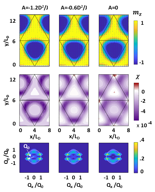
Figure 4: Evolution of magnetization texture, topological charge density $\chi$ and spin structure factor $I(Q)$ for $AJ/D^{2}=\{-1.2,-0.6,0\}$ at $L=8L_{D}$.

Next, we explore the effects of anisotropy, $A$ at around optimal angle $L=8L_{D}$ as shown in Fig. 3. At low exchange field, we obtain spiral phase for a wide range of $A$, a small ferromagnetic phase at lowest negative values of $A$ as well as a mixed (FM+Sp) phase at largest positive values of $A$. As the field increases, initially we get SkX near the lowest negative values of $A$ that corresponds to easy axis anisotropy. By further increasing the field, the range of SkX gradually increases and eventually, occupies the whole phase diagram. Fig. 3(b,c,d) show the local magnetization and Fig. 3(e,f,g) show the spin structure factor $I(Q)\propto|\langle\textbf{m}_{Q}\rangle|^{2}$ for the three phases. $\textbf{m}_{Q}$ is the Fourier transform of the magnetization. Unlike an isotropic SkX which has six peaks on the circle in the spin structure factor, we find four peaks lie on circle and two peaks lie inside the circle. This is due to the anisotropic triangular shape of the SkX. The spiral has two peaks at $Q=\pm Q_{0}$ and the mixed state (FM+Sp) has three peaks including the $Q=0$ from the FM and $Q=\pm Q_{0}$ from the spiral phase. The intensity of $Q=0$ peak increases with increasing $A$ and decreases with increasing exchange field $B_{Max}$. On the other hand, the intensities corresponding to the spiral wave vectors have the opposite behavior of $Q=0$ with $A$ and $B_{Max}$.
The properties of SkX also depends on the anisotropy $A$. Fig. 4 shows the magnetization, spin structure factor and topological charge density as a function of $A$ for moiré period $L=8L_{D}$. For $A=-1.2D^{2}/J$ the skyrmion has a sharp boundary wall where magnetization changes abruptly and then it changes slowly inside the skyrmion. The sharpness of boundary wall decreases with increasing $A$ and the change in magnetization inside the skyrmion increases with increasing $A$. For $A=-1.2D^{2}/J$, a large fraction of topological charge is concentrated at the boundary wall of skyrmion and a small fraction lies inside the skyrmion. There is also a small fraction of opposite charge between the skyrmions. The concentration of charge at boundary decreases with increasing $A$ and the central charge increases with increasing $A$. The fraction of opposite charge between the skyrmions also increases with increasing $A$Lin et al. (2015).

We also studied the effects of anisotropy for a non-optimal angle at $L=5L_{D}$. As shown in Fig. 5, SkX is highly suppressed in this case but still persists for large exchange field and easy axis anisotropy. Suppression of SkX is due to the fact that the moiré supercell is too small with respect to the optimal size of the skyrmions.

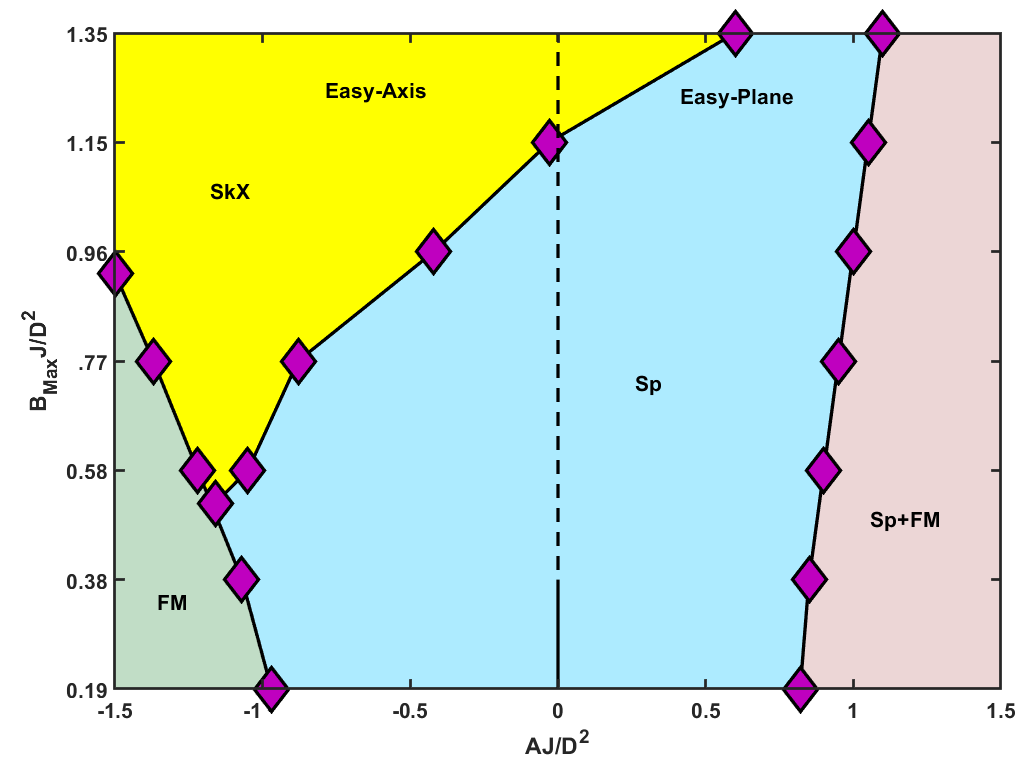
Figure 5: Anisotropy $A$ vs maximum interlayer exchange field $B_{Max}$ phase diagram with ferromagnetic (FM), spiral (Sp), skyrmion crystal (SkX) and mixed state (Sp+FM) phases at $L=5L_{D}$. Here $L_{D}=(J/D)a$, where $a$ is the lattice constant.

Our results apply to a wide range of vdW magnets since the primary constraint in our model is the requirement that $J_{ex}<J$ which is in general satisfied for vdW magnets. Our phase diagrams span a wide range of parameters and for a fixed twisting angle, our results scale with $AJ/D^{2}$.

IV Conclusion

We have shown that skyrmion crystal can be stabilized in moiré superlattices in the absence of external magnetic field. We found a large SkX phase for easy axis anisotropy which can be essential to stabilize skyrmions in vdW magnets such as CrI₃Huang et al. (2017). In particular, for optimal moiré periodicity SkX occupies the majority of the phase diagram. We find that the properties of the skyrmion can be tuned with the moiré periodicity and anisotropy. Unlike skyrmions in chiral magnets, the topological charge density depends on the size of the skyrmions sand it is concentrated at the edges for skyrmions with large L.

V Acknowledgements

We thank Sumilan Banerjee for useful discussions. MA is supported by Fulbright scholarship and ASU startup grant and OE is supported by NSF-DMR-1904716. We acknowledge the ASU Research Computing Center for HPC resources.

References

- Gibertini et al. (2019) M. Gibertini, M. Koperski, A. Morpurgo, and K. Novoselov, Nature Nanotechnology 14, 408 (2019).
- Gong and Zhang (2019) C. Gong and X. Zhang, Science 363, eaav4450 (2019).
- Burch et al. (2018) K. S. Burch, D. Mandrus, and J.-G. Park, Nature 563, 47 (2018).
- Huang et al. (2017) B. Huang, G. Clark, E. Navarro-Moratalla, D. R. Klein, R. Cheng, K. L. Seyler, D. Zhong, E. Schmidgall, M. A. McGuire, D. H. Cobden, et al., Nature 546, 270 (2017).
- Moriya (1960b) T. Moriya, Phys. Rev. 120, 91 (1960b).
- Gong et al. (2017) C. Gong, L. Li, Z. Li, H. Ji, A. Stern, Y. Xia, T. Cao, W. Bao, C. Wang, Y. Wang, et al., Nature 546, 265 (2017).
- Deng et al. (2018) Y. Deng, Y. Yu, Y. Song, J. Zhang, N. Z. Wang, Z. Sun, Y. Yi, Y. Z. Wu, S. Wu, J. Zhu, et al., Nature 563, 94 (2018).
- Bonilla et al. (2018) M. Bonilla, S. Kolekar, Y. Ma, H. C. Diaz, V. Kalappattil, R. Das, T. Eggers, H. R. Gutierrez, M.-H. Phan, and M. Batzill, Nature Nanotechnology 13, 289 (2018).
- O’Hara et al. (2018) D. J. O’Hara, T. Zhu, A. H. Trout, A. S. Ahmed, Y. K. Luo, C. H. Lee, M. R. Brenner, S. Rajan, J. A. Gupta, D. W. McComb, et al., Nano Letters 18, 3125 (2018).
- Soriano et al. (2019) D. Soriano, C. Cardoso, and J. Fernández-Rossier, Solid State Communications 299, 113662 (2019).
- Cristoloveanu et al. (2019) S. Cristoloveanu, K. H. Lee, H. Park, and M. S. Parihar, Solid-State Electronics 155, 32 (2019).
- Ye et al. (2012) J. Ye, Y. J. Zhang, R. Akashi, M. S. Bahramy, R. Arita, and Y. Iwasa, Science 338, 1193 (2012).
- Cao et al. (2018a) Y. Cao, V. Fatemi, S. Fang, K. Watanabe, T. Taniguchi, E. Kaxiras, and P. Jarillo-Herrero, Nature 556, 43 (2018a).
- Huang et al. (2018) B. Huang, G. Clark, D. R. Klein, D. MacNeill, E. Navarro-Moratalla, K. L. Seyler, N. Wilson, M. A. McGuire, D. H. Cobden, D. Xiao, et al., Nature Nanotechnology 13, 544 (2018).
- Song et al. (2019) T. Song, Z. Fei, M. Yankowitz, Z. Lin, Q. Jiang, K. Hwangbo, Q. Zhang, B. Sun, T. Taniguchi, K. Watanabe, et al., Nature Materials 18, 1 (2019).
- Ponomarenko et al. (2013) L. Ponomarenko, R. Gorbachev, G. Yu, D. Elias, R. Jalil, A. Patel, A. Mishchenko, A. Mayorov, C. Woods, J. Wallbank, et al., Nature 497, 594 (2013).
- Dean et al. (2013) C. R. Dean, L. Wang, P. Maher, C. Forsythe, F. Ghahari, Y. Gao, J. Katoch, M. Ishigami, P. Moon, M. Koshino, et al., Nature 497, 598 (2013).
- Gorbachev et al. (2014) R. Gorbachev, J. Song, G. Yu, A. Kretinin, F. Withers, Y. Cao, A. Mishchenko, I. Grigorieva, K. Novoselov, L. Levitov, et al., Science 346, 448 (2014).
- Cao et al. (2018b) Y. Cao, V. Fatemi, A. Demir, S. Fang, S. L. Tomarken, J. Y. Luo, J. D. Sanchez-Yamagishi, K. Watanabe, T. Taniguchi, E. Kaxiras, et al., Nature 556, 80 (2018b).
- Zhang et al. (2017) C. Zhang, C.-P. Chuu, X. Ren, M.-Y. Li, L.-J. Li, C. Jin, M.-Y. Chou, and C.-K. Shih, Science Advances 3, e1601459 (2017).
- Moon and Koshino (2014) P. Moon and M. Koshino, Physical Review B 90, 155406 (2014).
- Chen et al. (2019a) G. Chen, L. Jiang, S. Wu, B. Lyu, H. Li, B. L. Chittari, K. Watanabe, T. Taniguchi, Z. Shi, J. Jung, et al., Nature Physics 15, 237 (2019a).
- Chen et al. (2019b) G. Chen, A. L. Sharpe, P. Gallagher, I. T. Rosen, E. J. Fox, L. Jiang, B. Lyu, H. Li, K. Watanabe, T. Taniguchi, et al., Nature 572, 215 (2019b).
- Wallbank et al. (2015) J. R. Wallbank, M. Mucha-Kruczyński, X. Chen, and V. I. Fal’ko, Annalen der Physik 527, 359 (2015).
- Ni et al. (2015) G. Ni, H. Wang, J. Wu, Z. Fei, M. Goldflam, F. Keilmann, B. Özyilmaz, A. C. Neto, X. Xie, M. Fogler, et al., Nature Materials 14, 1217 (2015).
- Chen et al. (2019c) W. Chen, Z. Sun, Z. Wang, L. Gu, X. Xu, S. Wu, and C. Gao, Science 366, 983 (2019c).
- Sivadas et al. (2018) N. Sivadas, S. Okamoto, X. Xu, C. J. Fennie, and D. Xiao, Nano Letters 18, 7658 (2018).
- Jiang et al. (2019) P. Jiang, C. Wang, D. Chen, Z. Zhong, Z. Yuan, Z.-Y. Lu, and W. Ji, Phys. Rev. B 99, 144401 (2019).
- Du et al. (2016) K.-z. Du, X.-z. Wang, Y. Liu, P. Hu, M. I. B. Utama, C. K. Gan, Q. Xiong, and C. Kloc, ACS Nano 10, 1738 (2016).
- Klein et al. (2018) D. R. Klein, D. MacNeill, J. L. Lado, D. Soriano, E. Navarro-Moratalla, K. Watanabe, T. Taniguchi, S. Manni, P. Canfield, J. Fernández-Rossier, et al., Science 360, 1218 (2018).
- Tong et al. (2018) Q. Tong, F. Liu, J. Xiao, and W. Yao, Nano Letters 18, 7194 (2018).
- Roessler et al. (2006) U. K. Roessler, A. Bogdanov, and C. Pfleiderer, Nature 442, 797 (2006).
- Mühlbauer et al. (2009) S. Mühlbauer, B. Binz, F. Jonietz, C. Pfleiderer, A. Rosch, A. Neubauer, R. Georgii, and P. Böni, Science 323, 915 (2009).
- Yu et al. (2010) X. Yu, Y. Onose, N. Kanazawa, J. Park, J. Han, Y. Matsui, N. Nagaosa, and Y. Tokura, Nature 465, 901 (2010).
- Münzer et al. (2010) W. Münzer, A. Neubauer, T. Adams, S. Mühlbauer, C. Franz, F. Jonietz, R. Georgii, P. Böni, B. Pedersen, M. Schmidt, et al., Physical Review B 81, 041203 (2010).
- Yu et al. (2011) X. Yu, N. Kanazawa, Y. Onose, K. Kimoto, W. Zhang, S. Ishiwata, Y. Matsui, and Y. Tokura, Nature Materials 10, 106 (2011).
- Hamamoto et al. (2015) K. Hamamoto, M. Ezawa, and N. Nagaosa, Physical Review B 92, 115417 (2015).
- Shiomi et al. (2013) Y. Shiomi, N. Kanazawa, K. Shibata, Y. Onose, and Y. Tokura, Physical Review B 88, 064409 (2013).
- Fert et al. (2013) A. Fert, V. Cros, and J. Sampaio, Nature Nanotechnology 8, 152 (2013).
- Banerjee et al. (2014) S. Banerjee, J. Rowland, O. Erten, and M. Randeria, Physical Review X 4, 031045 (2014).
- Johnson et al. (1996) M. Johnson, P. Bloemen, F. Den Broeder, and J. De Vries, Reports on Progress in Physics 59, 1409 (1996).
- Dubowik (1996) J. Dubowik, Physical Review B 54, 1088 (1996).
- Banerjee et al. (2013) S. Banerjee, O. Erten, and M. Randeria, Nature Physics 9, 626 (2013).
- Levy and Fert (1981) P. M. Levy and A. Fert, Phys. Rev. B 23, 4667 (1981).
- Fert and Levy (1980) A. Fert and P. M. Levy, Phys. Rev. Lett. 44, 1538 (1980).
- Gilbert (2004) T. L. Gilbert, IEEE Transactions on Magnetics 40, 3443 (2004).
- Hejazi et al. (2020) K. Hejazi, Z.-X. Luo, and L. Balents, arXiv:2009.00860, (2020).
- d’Aquino et al. (2005) M. d’Aquino, C. Serpico, G. Miano, I. Mayergoyz, and G. Bertotti, Journal of applied physics 97, 10E319 (2005).
- Lin et al. (2015) S.-Z. Lin, A. Saxena, and C. D. Batista, Physical Review B 91, 224407 (2015).