A sufficient condition for asymptotic stability of kinks in general (1+1)-scalar field models

Abstract.

We study stability properties of kinks for the (1+1)-dimensional nonlinear scalar field theory models

$$\partial_{t}^{2}\phi-\partial_{x}^{2}\phi+W^{\prime}(\phi)=0,\quad(t,x)\in\mathbb{R}\times\mathbb{R}.$$

The orbital stability of kinks under general assumptions on the potential $W$ is a consequence of energy arguments. Our main result is the derivation of a simple and explicit sufficient condition on the potential $W$ for the asymptotic stability of a given kink. This condition applies to any static or moving kink, in particular no symmetry assumption is required. Last, motivated by the Physics literature, we present applications of the criterion to the $P(\phi)_{2}$ theories and the double sine-Gordon theory.

1. Introduction

1.1. General setting

This article is concerned with the stability of kinks for general (1+1)-dimensional nonlinear scalar field theory models

$$\partial_{t}^{2}\phi-\partial_{x}^{2}\phi+W^{\prime}(\phi)=0,\quad(t,x)\in\mathbb{R}\times\mathbb{R}.$$ (1.1)

This model rewrites as a first order system for $\boldsymbol{\phi}=(\phi,\partial_{t}\phi)=(\phi_{1},\phi_{2})$

$$\begin{cases}\partial_{t}\phi_{1}=\phi_{2}\\ \partial_{t}\phi_{2}=\partial_{x}^{2}\phi_{1}-W^{\prime}(\phi_{1}).\end{cases}$$ (1.2)

The assumptions on the potential $W$ are standard

$$\begin{cases}\mbox{$W:\mathbb{R}\to[0,\infty)$ is of class $\mathcal{C}^{3}$,}\\ \mbox{$W$ has at least two zeros $\zeta_{-},\zeta_{+}\in\mathbb{R}$ such that $\zeta_{-}<\zeta_{+}$,}\\ \mbox{$W^{\prime}(\zeta_{\pm})=0$, $W^{\prime\prime}(\zeta_{\pm})>0$, and $W>0$ on $(\zeta_{-},\zeta_{+})$.}\end{cases}$$ (1.3)

Such assumptions ensure that (1.1) admits a kink corresponding to the heteroclinic orbit of the equation $h^{\prime\prime}=W^{\prime}(h)$ connecting the two consecutive vacua $\zeta_{-}$ and $\zeta_{+}$, and whose main properties are gathered in the following statement (see §2.1 for a proof and further properties).

Lemma 1.1 (Static kink).

Assume (1.3). There exists a solution $H$ of class $\mathcal{C}^{4}$ of the equation

$$\begin{cases}H^{\prime\prime}=W^{\prime}(H)\mbox{ on $\mathbb{R}$},\\ \lim_{-\infty}H=\zeta_{-},\quad\lim_{+\infty}H=\zeta_{+},\end{cases}$$

unique up to translation, which satisfies $H^{\prime}>0$ on $\mathbb{R}$. Moreover, there exist $C>0$ and $\omega>0$ such that for any $k=1,2,3,4$,

$$|H(x)-\zeta_{\pm}|\leq Ce^{\mp\omega x},\quad|H^{(k)}(x)|\leq Ce^{-\omega|x|}\quad\mbox{on $\mathbb{R}$}.$$ (1.4)

The solution $\boldsymbol{H}=(H,0)$ of (1.2) is called the static kink. For $c\in(-1,1)$ we define $\gamma=\gamma(c)\in[1,\infty)$ and the functions $H_{c}$, $\boldsymbol{H}_{c}$ by

$$\gamma=\frac{1}{\sqrt{1-c^{2}}},\quad H_{c}(x)=H(\gamma x),\quad\boldsymbol{H}_{c}(x)=\begin{pmatrix}H_{c}(x)\\[2.0pt] -cH^{\prime}_{c}(x)\end{pmatrix}.$$

The Lorentz boosted versions of the kink are defined by $\boldsymbol{\phi}(t,x)=\boldsymbol{H}_{c}(x-ct)$, for any $c\in(-1,1)$. These solutions, together with their translated versions, form the kink family of the model (1.2) related to the consecutive wells $\zeta_{-}$, $\zeta_{+}$ of the potential $W$.

Recall the conservation laws of the model

$$\mathcal{E}[\boldsymbol{\phi}] =\frac{1}{2}\int\left[\phi_{2}^{2}+(\partial_{x}\phi_{1})^{2}+2W(\phi_{1})\right],$$ (Energy)

$$\mathcal{P}[\boldsymbol{\phi}] =\int\phi_{2}\partial_{x}\phi_{1}.$$ (Momentum)

Since $W\geq 0$ on $\mathbb{R}$, the set of functions $\boldsymbol{\phi}\in L^{1}_{\rm loc}(\mathbb{R})\times L^{1}_{\rm loc}(\mathbb{R})$ for which the energy is finite is

$$\boldsymbol{E}=\left\{\boldsymbol{\phi}\in L^{1}_{\rm loc}(\mathbb{R})\times L^{1}_{\rm loc}(\mathbb{R}):\partial_{x}\phi_{1}\in L^{2}(\mathbb{R}),\ \sqrt{W(\phi_{1})}\in L^{2}(\mathbb{R}),\ \phi_{2}\in L^{2}(\mathbb{R})\right\}.$$

To study the stability of $\boldsymbol{H}$, we introduce the following subset $\boldsymbol{E}_{\boldsymbol{H}}$ of $\boldsymbol{E}$

$$\boldsymbol{E}_{\boldsymbol{H}}=\left\{\boldsymbol{\phi}\in\boldsymbol{E}:\boldsymbol{\phi}-\boldsymbol{H}\in H^{1}(\mathbb{R})\times L^{2}(\mathbb{R})\right\}.$$

By the properties of $W$ in (1.3) and Lemma 1.1, we observe that

$$\boldsymbol{E}_{\boldsymbol{H}}=\left\{\boldsymbol{\phi}\in L^{1}_{\rm loc}(\mathbb{R})\times L^{1}_{\rm loc}(\mathbb{R}):\partial_{x}\phi_{1}\in L^{2}(\mathbb{R}),\ \phi_{1}-H\in L^{2}(\mathbb{R}),\ \phi_{2}\in L^{2}(\mathbb{R})\right\}.$$

For $c\in(-1,1)$ and $\boldsymbol{v}=(v_{1},v_{2})\in H^{1}(\mathbb{R})\times L^{2}(\mathbb{R})$, we set

$$\left\|\boldsymbol{v}\right\|_{c}^{2}=\gamma^{-1}\left\|\partial_{x}v_{1}\right\|_{L^{2}}^{2}+\gamma\left\|v_{1}\right\|_{L^{2}}^{2}+\gamma\left\|v_{2}+c\partial_{x}v_{1}\right\|_{L^{2}}^{2},$$

and for $R>0$,

$$\left\|\boldsymbol{v}\right\|_{c,R}^{2}=\gamma^{-1}\left\|\partial_{x}v_{1}\right\|_{L^{2}(|x|<R)}^{2}+\gamma\left\|v_{1}\right\|_{L^{2}(|x|<R)}^{2}+\gamma\left\|v_{2}+c\partial_{x}v_{1}\right\|_{L^{2}(|x|<R)}^{2}.$$

1.2. Main results

For the sake of completeness, we state the result of orbital stability of the kink family in the general context (1.3). The proof given in Sections 2 and 3 relies on standard energy arguments; see also [32, 55].

Theorem 1 (Orbital stability).

Assume (1.3). There exist $\delta_{*}>0$ and $C_{*}>0$ such that for any $c_{0}\in(-1,1)$ and any $\boldsymbol{\phi}^{in}\in\boldsymbol{E}_{\boldsymbol{H}}$ with

$$\left\|\boldsymbol{\phi}^{in}-\boldsymbol{H}_{c_{0}}\right\|_{c_{0}}\leq\delta_{*},$$

there exists a unique global solution $\boldsymbol{\phi}\in\mathcal{C}(\mathbb{R},\boldsymbol{E}_{\boldsymbol{H}})$ of (1.1) with $\boldsymbol{\phi}(0)=\boldsymbol{\phi}^{in}$. Moreover, for all $t\in\mathbb{R}$

$$\inf_{y\in\mathbb{R}}\left\|\boldsymbol{\phi}(t,\cdot+y)-\boldsymbol{H}_{c_{0}}\right\|_{c_{0}}\leq C_{*}\left\|\boldsymbol{\phi}^{in}-\boldsymbol{H}_{c_{0}}\right\|_{c_{0}}.$$

Remark 1.1.

In the statement of Theorem 1, the constants $\delta_{*}$ and $C_{*}$ are independent of the speed $c_{0}$ of the kink. To state such an optimal stability result, one has to use the norm $\|\cdot\|_{c_{0}}$. Moreover, while equivalent to $\|\cdot\|_{H^{1}\times L^{2}}$, this norm seems more natural since it measures the perturbation in the moving frame of the kink: if $\boldsymbol{\phi}$ is a Lorentz boosted version of the kink with speed $c$, then $\phi_{2}+c\partial_{x}\phi_{1}=0$.

We turn to the notion of asymptotic stability.

Definition 1 (Asymptotic stability).

Assume (1.3). The kink $H$ is said to be asymptotically stable if for any $c_{0}\in(-1,1)$ there exists $\delta_{0}\in(0,\delta_{*}]$ such that for any $\boldsymbol{\phi}^{in}\in\boldsymbol{E}_{\boldsymbol{H}}$ with

$$\left\|\boldsymbol{\phi}^{in}-\boldsymbol{H}_{c_{0}}\right\|_{c_{0}}\leq\delta_{0},$$

there exist $c_{-},c_{+}\in(-1,1)$ and a $\mathcal{C}^{1}$ function $y:\mathbb{R}\to\mathbb{R}$ with $\lim_{t\to\pm\infty}\dot{y}(t)=c_{\pm}$, such that the global solution $\boldsymbol{\phi}$ of (1.1) with $\boldsymbol{\phi}(0)=\boldsymbol{\phi}^{in}$ satisfies, for any $R>0$

$$\lim_{t\to\pm\infty}\|\boldsymbol{\phi}(t,\cdot+y(t))-\boldsymbol{H}_{c_{\pm}}\|_{c_{\pm},R}=0.$$

This definition gives a strong notion of asymptotic completeness of the family of kinks defined from $H$, requiring that any translated and Lorentz boosted version of the kink is asymptotically stable, under any small perturbation in the energy space. In this definition, the solution $\boldsymbol{\phi}(t)$ approaches as $t\to\pm\infty$ the final moving kinks $\boldsymbol{H}_{c_{\pm}}(x-y(t))$ locally in space around the time-dependent kink position $y(t)$.

The goal of this article is to exhibit a simple and general sufficient condition on the potential $W$ for asymptotic stability, without assuming any symmetry property for the potential nor for the kink. To formulate the condition, we introduce the transformed potential $V:(\zeta_{-},\zeta_{+})\to\mathbb{R}$ defined by

$$V=-W\left(\log W\right)^{\prime\prime}.$$ (1.5)

The main result of this article is the following theorem, proved in Section 4.

Theorem 2 (Sufficient condition for asymptotic stability).

Assume (1.3). If the transformed potential $V$ satisfies $V^{\prime}\not\equiv 0$ on $(\zeta_{-},\zeta_{+})$ and

there exists $$\zeta_{0}\in[\zeta_{-},\zeta_{+}] (\phi-\zeta_{0})V^{\prime}(\phi)\leq 0 \phi\in(\zeta_{-},\zeta_{+})$$ such that for all , (1.6)

then the kink $H$ is asymptotically stable.

Remark 1.2.

From the orbital stability result, in the context of Theorem 2, it also holds, for a constant $C>0$

$$\gamma_{0}^{2}\sup_{t\in\mathbb{R}}|\dot{y}(t)-c_{0}|+\gamma_{0}^{2}|c_{\pm}-c_{0}|\leq C\left\|\boldsymbol{\phi}^{in}-\boldsymbol{H}_{c_{0}}\right\|_{c_{0}}.$$

Moreover, the proof of Theorem 2 yields the following information: there exists a $\mathcal{C}^{1}$ function $c:\mathbb{R}\to(-1,1)$ satisfying

$$\lim_{\pm\infty}c=c_{\pm}\quad\mbox{and}\quad\sup_{t\in\mathbb{R}}|\dot{c}(t)-c_{0}|\leq C\left\|\boldsymbol{\phi}^{in}-\boldsymbol{H}_{c_{0}}\right\|_{c_{0}},$$

and such that, for any $R>0$

$$\int_{-\infty}^{+\infty}\|\boldsymbol{\phi}(t,\cdot+y(t))-\boldsymbol{H}_{c(t)}\|_{(H^{1}\times L^{2})(|x|<R)}^{2}\,\textnormal{d}t<\infty.$$ (1.7)

The sufficient condition (1.6) is related to the repulsivity of the potential $V(H)$ (see Lemma 2.1) that appears after transformation by factorization of the linearized equation around the kink. This condition implies that the model does not have internal mode nor resonance for the kink $H$, which are known spectral obstructions for estimates of the form (1.7). The factorization procedure is a key tool of the proof of Theorem 2. We refer to §4.2 for its heuristic presentation and a more technical discussion on the condition (1.6).

Interestingly, one easily checks that the transformed potential is constant for the (integrable) sine-Gordon equation corresponding to the potential

$$W_{\textnormal{sG}}(\phi)=1-\cos\phi.$$ (1.8)

The converse statement is established in §5.2. This threshold situation $V^{\prime}\equiv 0$ is excluded by Theorem 2, which is consistent with the fact that the kink of the sine-Gordon equation is not asymptotically stable in the sense of Definition 1 (see references in §1.3). This observation also motivates the study of some models approximating the sine-Gordon equation; see below and §5.

For the $\phi^{4}$ model, corresponding to the potential

$$W_{4}(\phi)=(\phi^{2}-1)^{2},$$ (1.9)

the asymptotic stability of the kink is usually conjectured but seems very challenging to prove in general mainly because of the presence of one even resonance and one odd internal mode. In particular, the condition (1.6) does not hold for the $\phi^{4}$ model (see §5.3.1) and Theorem 2 is inconclusive in this case. However, the main result in [41] establishes the asymptotic stability of the static kink in the case of odd perturbations, avoiding the resonance, but taking into account the internal mode. In the same context, for odd initial data in weighted spaces, a very recent result [23] shows refined decay estimates on the solution, up to a time of size $\delta_{0}^{-\beta}$, where $\delta_{0}$ is the size of the initial perturbation and $\beta$ is any number less than $4$.

The above two classical models contain the main obstructions and difficulties encountered in addressing asymptotic stability and continue to be great challenges.

This being said, we point out that Theorem 2 allows us to prove new results of asymptotic stability for several models from the Physics literature. In Section 5, the sufficient condition (1.6) is first checked for the $\phi^{6}$ model

$$W_{6}(\phi)=\phi^{2}(\phi^{2}-1)^{2},$$ (1.10)

(see Theorem 4) and then for generalized versions of the $\phi^{4n}$ and $\phi^{4n+2}$ models for a large range of parameters (see Theorems 5, 6 and 7). It is also striking that Theorem 2 implies asymptotic stability of kinks for several approximations of the sine-Gordon equation in the $P(\phi)_{2}$ and double sine-Gordon theories, arbitrarily close to the sine-Gordon model (see Theorems 8, 9 and 10).

1.3. References

The Physics literature provides many references motivating the mathematical study of the dynamical properties of kinks for one-dimensional scalar field models (see e.g. [18, 29, 35, 48, 56, 64, 74, 75, 77]). Two articles have especially motivated the applications considered in Section 5: [55] for the $P(\phi)_{2}$ theories, and  [9] for the double sine-Gordon model (see also [5, 26, 36]).

Basic properties and orbital stability of kinks for general scalar field models were studied in several previous articles, such as [3, 32, 33, 55].

The results stated in Section 5, together with results in [2, 23, 41] concern the asymptotic stability of kinks for the $P(\phi)_{2}$ and double sine-Gordon theories. Previous works are devoted to asymptotic stability for various related models.

First, the question is similar to the asymptotic stability of the solitons of the nonlinear focusing Klein-Gordon equation, addressed in [6, 44, 46].

Second, several authors have considered the model (1.1) under different assumptions on the potential. In [39, 40], the authors consider natural spectral assumptions (absence of resonance, knowledge of internal modes) but they also need a more technical flatness condition of the potential near the wells (related to assumptions in [7, 8]). Moreover, initial data in [39, 40] are taken in weighted spaces. A three-dimensional version of the $\phi^{4}$ model is studied in [12], using dispersive estimates for free solutions available in higher space dimensions.

The sine-Gordon model has been the object of many studies, mainly due to its physical relevance and integrable structure (see the general references above). Recall from [17] that exceptional periodic solutions called wobbling kinks arbitrarily close to the kink, are obstacle to the asymptotic stability of the kink in the energy space. However, there is no known obstruction to asymptotic stability in a different topology (this corrects [41, End of Remark 1.3]). We refer to [2] for asymptotic stability of the kink for perturbations with symmetry.

For the sine-Gordon and the $\phi^{4}$ models, breathers, kink-antikink solutions and multi-solitons were studied mathematically in [1, 34, 62]. Other results concern the nonexistence of breathers for nonintegrable models [24, 42, 47, 69].

More generally, the asymptotic stability of kinks is closely related to the asymptotic behavior of small solutions of nonlinear Klein-Gordon or wave-type equations, which has been studied by many different techniques and various authors, for constant or variable coefficients. Pioneering works on the subject are [37, 38, 70, 71, 72, 19]. We also refer to [20, 22, 4, 23, 27, 30, 31, 49, 50, 51, 52, 53, 73] for notable progress on this question, in different directions. For the special case of the wave equation in one dimension, we refer to [54, 78].

Last, recall that the question of the asymptotic stability of solitary waves has been addressed by various techniques for nonlinear dispersive models, like the generalized Korteweg de Vries equation (generalization of the classical KdV equation) and variants of the nonlinear Schrödinger equation, with or without potential, which have some analogy with the models considered here. We briefly quote some results and refer to the review [43] for more references. The techniques used and developed in the present paper are partly reminiscent of the ones introduced in [57, 58, 59, 60] to prove the asymptotic stability of the solitons of the gKdV equations. See also [11] for an extension to a 2-dimensional variant of this model. Recall that the first result on such problem was obtained in [63] by different methods. Still different techniques, involving the special algebraic structure of the modified KdV equation and refined linear estimates were used in [28]. For the nonlinear Schrödinger equations, we mention the pioneering articles [7, 8] and [13, 14, 15, 21, 45, 67, 68, 76], as well as [16] concerning the integrable case. See also [25, 61] in the blow up context. The article [79] concerns kinks of nonlinear Schrödinger equations.

For the proof of Theorem 2, we follow and develop the approach to asymptotic stability of kinks and solitons for wave-type equations initiated in [41] and [44]. In particular, we adapt the method to the case of initial data without symmetry and non zero speed. We emphasize that the articles [10, 57, 58, 60, 65] for the nonlinear Schrödinger equations, the generalized KdV equations and the wave maps were also inspiring for this approach.

2. Modulation around the kink family

In this section, we study the neighborhood of kinks. This includes the expansion of the conservation laws around the kink, the study of the linearized operator and a decomposition result around the kink family by modulation.

2.1. Preliminary observations about the potential and the kink

First, we provide a proof of Lemma 1.1, containing standard information on the kink (see also [32, 34]). Set

$$\omega_{-}=\sqrt{W^{\prime\prime}(\zeta_{-})},\quad\omega_{+}=\sqrt{W^{\prime\prime}(\zeta_{-})},\quad\omega=\min(\omega_{-};\omega_{+})>0.$$ (2.1)

Proof of Lemma 1.1.

We integrate explicitly the equation $H^{\prime\prime}=W^{\prime}(H)$ after multiplication by $H^{\prime}$ as $(H^{\prime})^{2}=2W(H)$. We obtain $G(H(x))=x$, where the function $G:(\zeta_{-},\zeta_{+})\to\mathbb{R}$ is defined by

$$G(h)=\int_{\zeta_{0}}^{h}\frac{\,\textnormal{d}s}{\sqrt{2W(s)}},\quad\zeta_{0}=\frac{\zeta_{-}+\zeta_{+}}{2}.$$ (2.2)

The invariance by translation of the equation is handled by the arbitrary choice $H(0)=\zeta_{0}$. Note that by the assumptions (1.3) on $W$ and the Taylor expansion at the points $\zeta_{\pm}$, we have for $s\sim\zeta_{\pm}$,

$$W(s)=\frac{W^{\prime\prime}(\zeta_{\pm})}{2!}(s-\zeta_{\pm})^{2}+\frac{W^{\prime\prime\prime}(\zeta_{\pm})}{3!}(s-\zeta_{\pm})^{3}+o\left((s-\zeta_{\pm})^{3}\right).$$ (2.3)

In particular, it holds

$$\frac{1}{\sqrt{2W(s)}}=\frac{1}{\sqrt{W^{\prime\prime}(\zeta_{\pm})}}\frac{1}{|s-\zeta_{\pm}|}\left(1-\frac{1}{6}\frac{W^{\prime\prime\prime}(\zeta_{\pm})}{W^{\prime\prime}(\zeta_{\pm})}(s-\zeta_{\pm})+o(s-\zeta_{\pm})\right).$$

This justifies that $G$ is an increasing one-to-one map from $(\zeta_{-},\zeta_{+})$ to $\mathbb{R}$. Thus, $H$ is uniquely defined on $\mathbb{R}$ by $H(x)=G^{-1}(x)$. Moreover, by integration of the above Taylor expansion, one has

$$G(h)=\mp\frac{1}{\sqrt{W^{\prime\prime}(\zeta_{\pm})}}\log|h-\zeta_{\pm}|+C_{\pm}+C_{\pm}^{\prime}(h-\zeta_{\pm})+o(h-\zeta_{\pm}),$$

for some constants $C_{\pm}$ and $C_{\pm}^{\prime}$. Using $G(H(x))=x$, this gives

$$x=\mp\frac{1}{\sqrt{W^{\prime\prime}(\zeta_{\pm})}}\log|H(x)-\zeta_{\pm}|+C_{\pm}+C_{\pm}^{\prime}(H(x)-\zeta_{\pm})+o(H(x)-\zeta_{\pm}).$$

It follows that for two positive constants $\lambda_{\pm}$,

$$H(x)=\zeta_{\pm}\mp\lambda_{\pm}e^{\mp\omega_{\pm}x}+O\left(e^{\pm 2\omega_{\pm}x}\right)\quad\mbox{as $x\to\pm\infty$.}$$ (2.4)

Using $H^{\prime}(x)=\sqrt{2W(H(x))}$, (2.3) and (2.4) we also obtain

$$H^{\prime}(x)=\omega_{\pm}\lambda_{\pm}e^{\mp\omega_{\pm}x}+O\left(e^{\mp 2\omega_{\pm}x}\right)\quad\mbox{as $x\to\pm\infty$.}$$ (2.5)

By the equation $H^{\prime\prime}=W^{\prime}(H)$ and the $\mathcal{C}^{3}$ regularity of $W$, it is clear that $H$ is of class $\mathcal{C}^{4}$ and $H^{\prime\prime\prime}=H^{\prime}W^{\prime\prime}(H)$, $H^{(4)}=H^{\prime\prime}W^{\prime\prime}(H)+H^{\prime 2}W^{\prime\prime\prime}(H)$. Moreover, by Taylor expansions of $W^{\prime}$, $W^{\prime\prime}$ and $W^{\prime\prime\prime}$ near $\zeta_{\pm}$, it holds

$$H^{\prime\prime}(x) =\mp\omega_{\pm}^{2}\lambda_{\pm}e^{\mp\omega_{\pm}x}+O\left(e^{\mp 2\omega_{\pm}x}\right),$$ (2.6)

$$H^{\prime\prime\prime}(x) =\omega_{\pm}^{3}\lambda_{\pm}e^{\mp\omega_{\pm}x}+O\left(e^{\mp 2\omega_{\pm}x}\right),$$

$$H^{(4)}(x) =\mp\omega_{\pm}^{4}\lambda_{\pm}e^{\mp\omega_{\pm}x}+O\left(e^{\mp 2\omega_{\pm}x}\right).$$

In particular, $H^{\prime\prime}/H^{\prime}$ is bounded on $\mathbb{R}$. Another observation is

$$|W^{\prime\prime}(H(x))-\omega_{\pm}^{2}|\leq Ce^{\mp\omega_{\pm}x}.$$

This completes the proof of the lemma. ∎

Second, we observe that the sufficient condition for asymptotic stability (1.6) on the potential $V$ is a reformulation of the condition that will actually be used in this paper. The formulation (1.6) is privileged in our presentation since it can be checked directly on the potential $W$, without using the expression of the kink $H$.

Lemma 2.1.

Let $P:\mathbb{R}\to\mathbb{R}$ be the function of class $\mathcal{C}^{1}$ defined by

$$P=\frac{(W^{\prime}(H))^{2}}{W(H)}-W^{\prime\prime}(H)=2\left(\frac{H^{\prime\prime}}{H^{\prime}}\right)^{2}-\frac{H^{\prime\prime\prime}}{H^{\prime}}=H^{\prime}\left(\frac{1}{H^{\prime}}\right)^{\prime\prime}.$$

The condition (1.6) on $V$ is equivalent to $P^{\prime}\not\equiv 0$ on $\mathbb{R}$ and $P$ satisfies one of the following

Repulsivity at a point:

there exists $x_{0}\in\mathbb{R}$ such that $(x-x_{0})P^{\prime}\leq 0$ on $\mathbb{R};$

Repulsivity at $-\infty$:

$P^{\prime}\leq 0$ on $\mathbb{R};$

Repulsivity at $+\infty$:

$P^{\prime}\geq 0$ on $\mathbb{R}$.

Moreover,

$$\lim_{\pm\infty}P=V(\zeta_{\pm})=W^{\prime\prime}(\zeta_{\pm})=\omega_{\pm}^{2}.$$ (2.7)

Proof.

The result follows from $P(x)=V(H(x))$ so that $P^{\prime}(x)=H^{\prime}(x)V^{\prime}(H(x))$ and the fact that $H^{\prime}>0$ on $\mathbb{R}$. The cases $\zeta_{0}=\zeta_{-}$ and $\zeta_{0}=\zeta_{+}$ in (1.6) correspond to the repulsivity of $P$ at $-\infty$ and $+\infty$, respectively. The case $\zeta_{0}\in(\zeta_{-},\zeta_{+})$ corresponds to the repulsivity of $P$ at the point $x_{0}=H^{-1}(\zeta_{0})\in\mathbb{R}$.

Last, it is direct from its definition (1.5) and Taylor expansion that $V$ extends by continuity to $[\zeta_{-},\zeta_{+}]$ and that (2.7) holds. ∎

Remark 2.1.

1. Recall that by the standard virial argument, this assumption on $P$ implies the absence of eigenvalues for the Schrödinger operator $L_{0}=-\partial_{x}^{2}+P$. See [66, Theorem XIII.60]. See also the discussion in §4.2.

2. Since we consider $H^{1}\times L^{2}$ perturbations of the kink, the potential $W$ only needs to be defined in a neighborhood of the interval $[\zeta_{+},\zeta_{-}]$. We also observe that the assumption (1.6) of Theorem 2 only concerns the values of $W$ on the range $(\zeta_{-},\zeta_{+})$ of the kink. For a potential having several kinks joining different zeros of the potential, the criterion (1.6) for asymptotic stability may hold or not depending on each kink. See examples in §5.3.

3. By convention, we have chosen to consider the increasing kink $H$ corresponding to the heteroclinic orbit of $H^{\prime\prime}=W^{\prime}(H)$ joining $\zeta_{-}$ to $\zeta_{+}$. One can use the change of variable $x\mapsto-x$ to treat the decreasing kink $H(-x)$.

4. To prove the stability result in Theorem 1, the assumption that $W$ is of class $\mathcal{C}^{2}$ is sufficient. For the asymptotic stability result Theorem 2, our method requires $\mathcal{C}^{3}$ regularity.

5. The non degeneracy assumption $W^{\prime\prime}(\zeta_{\pm})>0$ is needed for the exponential convergence of $H$ to its limits at $\pm\infty$. However, some models, such as special cases of the generalized $\phi^{8}$ model (see [35, p. 268]) and the double sine-Gordon model (see §5.6), involve degenerate potentials $W$, i.e. satisfying $W^{\prime\prime}(\zeta_{\pm})=0$. Such case would require a specific study, taking into account the lower decay rates of the kink at $\pm\infty$ and different spectral properties for the linearized operator.

For future reference, we also state and prove some decay properties for auxiliary functions that will be considered throughout the paper. Define the function $Q$ (to be used in §4.9) by

$$Q=\left(\log H^{\prime}\right)^{\prime\prime}.$$ (2.8)

Lemma 2.2.

The functions $P$ and $Q$ are of class $\mathcal{C}^{1}$ on $\mathbb{R}$ and satisfy

$$|P(x)-\omega_{\pm}^{2}|\leq Ce^{\mp\omega x},\quad|P^{\prime}(x)|\leq Ce^{-\omega|x|},$$ (2.9)

$$|Q(x)|+|Q^{\prime}(x)|\leq Ce^{-\omega|x|}.$$ (2.10)

Moreover, under hypothesis (1.6), $P\geq\omega^{2}$ on $\mathbb{R}$, where $\omega$ is defined in (2.1).

Proof.

The decay properties (2.10) and (2.9) follow directly from the definitions of $P$ and $Q$ and the asymptotics (2.5) and (2.6) on $H$. The last property is a consequence of Lemma 2.1. ∎

2.2. Notation and expansion of the conservation laws

We will use the following notation for functions $u,$ $v\in L^{2}$, $\boldsymbol{u}=(u_{1},u_{2})$, $\boldsymbol{v}=(v_{1},v_{2})\in L^{2}$,

$$\left\langle{u},{v}\right\rangle=\int u(x)v(x)\,\textnormal{d}x,\quad\left\langle{\boldsymbol{u}},{\boldsymbol{v}}\right\rangle=\int\left[u_{1}(x)v_{1}(x)+u_{2}(x)v_{2}(x)\right]\,\textnormal{d}x.$$

For $c\in(-1,1)$ and $y\in\mathbb{R}$, we define the functions $H_{c,y}$ and $\boldsymbol{H}_{c,y}$

$$H_{c,y}(x)=H_{c}(x-y),\quad\boldsymbol{H}_{c,y}(x)=\boldsymbol{H}_{c}(x-y).$$

Note that with this notation $H^{\prime}_{c,y}(x)=\gamma H^{\prime}\left(\gamma(x-y)\right)$.

Lemma 2.3.

For any $c\in(-1,1)$ and $y\in\mathbb{R}$, the following hold.

1. Conservation laws for the kink.

   $$\mathcal{E}[\boldsymbol{H}_{c,y}]=\gamma\|H^{\prime}\|_{L^{2}}^{2},\quad\mathcal{P}[\boldsymbol{H}_{c,y}]=-c\gamma\|H^{\prime}\|_{L^{2}}^{2}.$$

2. Expansion of the conservation laws around the kink. For any $\boldsymbol{u}=(u_{1},u_{2})$ such that $\|u_{1}\|_{L^{\infty}}\leq 1$,

   $$\mathcal{E}[\boldsymbol{H}_{c,y}+\boldsymbol{u}] =\mathcal{E}[\boldsymbol{H}_{c,y}]-c\int H_{c,y}^{\prime}(u_{2}-c\partial_{x}u_{1})$$

   $$\quad+\frac{1}{2}\left(\|u_{2}\|_{L^{2}}^{2}+\left\langle{L_{c,y}u_{1}},{u_{1}}\right\rangle+\mathcal{R}\right),$$ (2.11)

   $$\mathcal{P}[\boldsymbol{H}_{c,y}+\boldsymbol{u}] =\mathcal{P}[\boldsymbol{H}_{c,y}]+\int H_{c,y}^{\prime}(u_{2}-c\partial_{x}u_{1})+\mathcal{P}[\boldsymbol{u}],$$ (2.12)

   where

   $$L_{c,y}=-\partial_{x}^{2}+W^{\prime\prime}(H_{c,y}),$$ (2.13)

   and

   $$|\mathcal{R}|\leq C\|u_{1}\|_{L^{\infty}}\|u_{1}\|_{L^{2}}^{2},$$ (2.14)

   for some constant $C>0$.

Remark 2.2.

These computations motivate the use of the orthogonality relation

$$\int H_{c,y}^{\prime}(u_{2}-c\partial_{x}u_{1})=0\iff\left\langle{\boldsymbol{u}},{\begin{pmatrix}cH_{c,y}^{\prime\prime}\\ H_{c,y}^{\prime}\end{pmatrix}}\right\rangle=0.$$ (2.15)

Proof.

The proof of (1) follows from direct computations.

Proof of (2). First, we expand $\mathcal{E}[\boldsymbol{H}_{c,y}+\boldsymbol{u}]$ for $\boldsymbol{u}=(u_{1},u_{2})$. We have

$$\mathcal{E}[\boldsymbol{H}_{c,y}+\boldsymbol{u}]=\mathcal{E}[\boldsymbol{H}_{c,y}]+\int\left[-cH_{c,y}^{\prime}u_{2}+H_{c,y}^{\prime}\partial_{x}u_{1}+W^{\prime}(H_{c,y})u_{1}\right]\\ +\frac{1}{2}\int\left\{u_{2}^{2}+(\partial_{x}u_{1})^{2}+2\left[W(H_{c,y}+u_{1})-W(H_{c,y})-W^{\prime}(H_{c,y})u_{1}\right]\right\}.$$

Using integration by parts and $W^{\prime}(H_{c,y})=\gamma^{-2}H_{c,y}^{\prime\prime}$, we obtain

$$\int\left[-cH_{c,y}^{\prime}u_{2}+H_{c,y}^{\prime}\partial_{x}u_{1}+W^{\prime}(H_{c,y})u_{1}\right]=-c\int H_{c,y}^{\prime}(u_{2}-c\partial_{x}u_{1}).$$

For $u_{1}$ such that $\|u_{1}\|_{L^{\infty}}<1$, we have by the Taylor formula (recall that we assume the potential $W$ of class $\mathcal{C}^{3}$)

$$\left|W(H_{c,y}+u_{1})-W(H_{c,y})-W^{\prime}(H_{c,y})u_{1}-W^{\prime\prime}(H_{c,y})\frac{u_{1}^{2}}{2}\right|\leq C|u_{1}|^{3}$$

where $C=\frac{1}{6}\sup_{[-1+\zeta_{-},1+\zeta_{+}]}|W^{\prime\prime\prime}|$. This proves (2.11).

Second, we observe by a direct expansion

$$\mathcal{P}[\boldsymbol{H}_{c,y}+\boldsymbol{u}]=\mathcal{P}[\boldsymbol{H}_{c,y}]+\int\left(H_{c,y}^{\prime}u_{2}-cH_{c,y}^{\prime}\partial_{x}u_{1}\right)+\mathcal{P}[\boldsymbol{u}],$$

which is (2.12). ∎

2.3. Generalized null spaces

We introduce some more notation related to the kink family. Let

$$\boldsymbol{T}_{c,y}=-\partial_{y}\boldsymbol{H}_{c,y}=\boldsymbol{H}_{c,y}^{\prime},\quad\boldsymbol{D}_{c,y}=\partial_{c}\boldsymbol{H}_{c,y},$$

respectively related to translations and the Lorentz transform, given explicitly by

$$\boldsymbol{T}_{c,y}(x) :=\begin{pmatrix}H_{c,y}^{\prime}(x)\\ -cH_{c,y}^{\prime\prime}(x)\end{pmatrix},$$

$$\boldsymbol{D}_{c,y}(x) :=\begin{pmatrix}c\gamma^{2}(x-y)H_{c,y}^{\prime}(x)\\ -\gamma^{2}H_{c,y}^{\prime}(x)-c^{2}\gamma^{2}(x-y)H_{c,y}^{\prime\prime}(x)\end{pmatrix}.$$

We also define

$$\boldsymbol{G}_{c,y}=\boldsymbol{J}\boldsymbol{T}_{c,y},\quad\boldsymbol{F}_{c,y}=\boldsymbol{J}\boldsymbol{D}_{c,y}\quad\mbox{where}\quad\boldsymbol{J}=\begin{pmatrix}0&1\\ -1&0\end{pmatrix}.$$

Let

$$\boldsymbol{L}_{c,y}=\begin{pmatrix}L_{c,y}&-c\partial_{x}\\ c\partial_{x}&1\end{pmatrix},$$ (2.16)

so that

$$\left\langle{\boldsymbol{L}_{c,y}\boldsymbol{u}},{\boldsymbol{u}}\right\rangle=\|u_{2}\|_{L^{2}}^{2}+\left\langle{L_{c,y}u_{1}},{u_{1}}\right\rangle+2c\mathcal{P}[\boldsymbol{u}].$$ (2.17)

The following relations also motivate the introduction of $\boldsymbol{T}_{c,y}$ and $\boldsymbol{D}_{c,y}$.

Lemma 2.4.

It holds

$$\boldsymbol{L}_{c,y}\boldsymbol{T}_{c,y}=0,\quad\boldsymbol{L}_{c,y}\boldsymbol{D}_{c,y}=\boldsymbol{J}\boldsymbol{T}_{c,y},$$ (2.18)

$$\left\langle{\boldsymbol{D}_{c,y}},{\boldsymbol{G}_{c,y}}\right\rangle=-\left\langle{\boldsymbol{T}_{c,y}},{\boldsymbol{F}_{c,y}}\right\rangle=\gamma^{3}\left\|H^{\prime}\right\|_{L^{2}}^{2}.$$ (2.19)

Proof.

First, the statement $\boldsymbol{L}_{c,y}\boldsymbol{T}_{c,y}=0$ follows easily by differentiating in $x$ the relation $(1-c^{2})H_{c,y}^{\prime\prime}+W^{\prime}(H_{c,y})=0$. To compute $\boldsymbol{L}_{c,y}\boldsymbol{D}_{c,y}$, we use $\boldsymbol{L}_{c,y}\boldsymbol{T}_{c,y}=0$ and a commutator relation

$$\boldsymbol{L}_{c,y}\boldsymbol{D}_{c,y} =\gamma^{2}\boldsymbol{L}_{c,y}\left\{\begin{pmatrix}0\\ -H^{\prime}_{c,y}\end{pmatrix}+c(x-y)\boldsymbol{T}_{c,y}\right\}$$

$$=\gamma^{2}\begin{pmatrix}cH_{c,y}^{\prime\prime}\\ -H^{\prime}_{c,y}\end{pmatrix}+\gamma^{2}c\left[\boldsymbol{L}_{c,y},(x-y)\right]\boldsymbol{T}_{c,y}$$

$$=\gamma^{2}\begin{pmatrix}cH_{c,y}^{\prime\prime}\\ -H^{\prime}_{c,y}\end{pmatrix}+\gamma^{2}c\begin{pmatrix}-2\partial_{x}&-c\\ c&0\end{pmatrix}\boldsymbol{T}_{c,y}=\boldsymbol{J}\boldsymbol{T}_{c,y}.$$

The proof of (2.19) is elementary. ∎

Remark 2.3.

The functions $\boldsymbol{T}_{c,y}$ and $\boldsymbol{D}_{c,y}$ span the generalized null space of the operator $\boldsymbol{J}\boldsymbol{L}_{c,y}$, whereas the functions $\boldsymbol{G}_{c,y}$ and $\boldsymbol{F}_{c,y}$ span the generalized null space of $\boldsymbol{L}_{c,y}\boldsymbol{J}$. The function $\boldsymbol{G}_{c,y}$ is also related to the expansion of the invariant quantities in Lemma 2.3. See (2.15) in Remark 2.2. We refer to [39, 40] for the introduction of these functions.

For future reference, we also compute

$$\boldsymbol{A}_{c,y}=-\partial_{y}\boldsymbol{D}_{c,y}=\partial_{c}\boldsymbol{T}_{c,y}=\begin{pmatrix}c\gamma^{2}H^{\prime}_{c,y}+c\gamma^{2}(x-y)H^{\prime\prime}_{c,y}\\ -(1+c^{2})\gamma^{2}H^{\prime\prime}_{c,y}-c^{2}\gamma^{2}(x-y)H^{\prime\prime\prime}_{c,y}\end{pmatrix}$$

and

$$\boldsymbol{B}_{c,y}=\partial_{c}\boldsymbol{D}_{c,y}=\begin{pmatrix}\gamma^{4}(1+2c^{2})(x-y)H^{\prime}_{c,y}+c^{2}\gamma^{4}(x-y)^{2}H^{\prime\prime}_{c,y}\\ -3c\gamma^{4}H^{\prime}_{c,y}-c\gamma^{4}(3+2c^{2})(x-y)H^{\prime\prime}_{c,y}-c^{3}\gamma^{4}(x-y)^{2}H^{\prime\prime\prime}_{c,y}\end{pmatrix}.$$

2.4. Lorentz invariant conserved quantity

In addition to the energy $\mathcal{E}$ and momentum $\mathcal{P}$, we introduce the following Lorentzian invariant quantity $\mathcal{M}$

$$\mathcal{M}[\boldsymbol{\phi}]=\left(\mathcal{E}[\boldsymbol{\phi}]\right)^{2}-\left(\mathcal{P}[\boldsymbol{\phi}]\right)^{2}.$$

We continue the computations of Lemma 2.3.

Lemma 2.5.

For any $c\in(-1,1)$ and $y\in\mathbb{R}$, the following hold.

1. Conservation law for the kink.

   $$\mathcal{M}[\boldsymbol{H}_{c,y}]=\|H^{\prime}\|_{L^{2}}^{4}.$$

2. Expansion of the conservation law around the kink. For any $\boldsymbol{u}=(u_{1},u_{2})$ such that $\|u_{1}\|_{L^{\infty}}\leq 1$ and $\left\langle{\boldsymbol{u}},{\boldsymbol{G}_{c,y}}\right\rangle=0$, it holds

   $$\mathcal{M}[\boldsymbol{H}_{c,y}+\boldsymbol{u}]=\|H^{\prime}\|_{L^{2}}^{4}\\ +\left(\left\langle{\boldsymbol{L}_{c,y}\boldsymbol{u}},{\boldsymbol{u}}\right\rangle+\mathcal{R}\right)\left(\gamma\|H^{\prime}\|_{L^{2}}^{2}+\frac{1}{4}\left\langle{\boldsymbol{L}_{-c,y}\boldsymbol{u}},{\boldsymbol{u}}\right\rangle+\frac{1}{4}\mathcal{R}\right).$$ (2.20)

Remark 2.4.

The quantity $\mathcal{M}$ enjoys two remarkable properties: the value of $\mathcal{M}$ for a kink $\boldsymbol{H}_{c,y}$ does not depend on its speed $c$ and any kink is a critical point of $\mathcal{M}$.

Proof.

The first point is a direct consequence of (1) of Lemma 2.3. Using (1) of Lemma 2.3, (2.11), (2.12) and the orthogonality $\left\langle{\boldsymbol{u}},{\boldsymbol{G}_{c,y}}\right\rangle=0$, we recall that

$$\mathcal{E}[\boldsymbol{H}_{c,y}+\boldsymbol{u}] =\gamma\|H^{\prime}\|_{L^{2}}^{2}+\frac{1}{2}\left(\|u_{2}\|_{L^{2}}^{2}+\left\langle{L_{c,y}u_{1}},{u_{1}}\right\rangle+\mathcal{R}\right),$$

$$\mathcal{P}[\boldsymbol{H}_{c,y}+\boldsymbol{u}] =-c\gamma\|H^{\prime}\|_{L^{2}}^{2}+\mathcal{P}[\boldsymbol{u}].$$

As a consequence, we compute

$$\mathcal{M}[\boldsymbol{H}_{c,y}+\boldsymbol{u}] =\|H^{\prime}\|_{L^{2}}^{4}+\gamma\|H^{\prime}\|_{L^{2}}^{2}\left(\|u_{2}\|_{L^{2}}^{2}+\left\langle{L_{c,y}u_{1}},{u_{1}}\right\rangle+2c\mathcal{P}[\boldsymbol{u}]+\mathcal{R}\right)$$

$$\quad+\frac{1}{4}\left(\|u_{2}\|_{L^{2}}^{2}+\left\langle{L_{c,y}u_{1}},{u_{1}}\right\rangle+\mathcal{R}\right)^{2}-(\mathcal{P}[u])^{2}.$$

Using the expression of $\left\langle{\boldsymbol{L}_{c,y}\boldsymbol{u}},{\boldsymbol{u}}\right\rangle$ in (2.17), we write

$$\mathcal{M}[\boldsymbol{H}_{c,y}+\boldsymbol{u}] =\|H^{\prime}\|_{L^{2}}^{4}+\gamma\|H^{\prime}\|_{L^{2}}^{2}\left(\left\langle{\boldsymbol{L}_{c,y}\boldsymbol{u}},{\boldsymbol{u}}\right\rangle+\mathcal{R}\right)$$

$$\quad+\frac{1}{4}\left(\left\langle{\boldsymbol{L}_{c,y}\boldsymbol{u}},{\boldsymbol{u}}\right\rangle+\mathcal{R}\right)\left(\left\langle{\boldsymbol{L}_{-c,y}\boldsymbol{u}},{\boldsymbol{u}}\right\rangle+\mathcal{R}\right),$$

which is (2.20). To justify Remark 2.4, observe that even without the assumption $\left\langle{\boldsymbol{u}},{\boldsymbol{G}_{c,y}}\right\rangle=0$, the terms $\left\langle{\boldsymbol{u}},{\boldsymbol{G}_{c,y}}\right\rangle$ in (2.11) and (2.12) vanish at order $1$ in $\boldsymbol{u}$ in the expression of $\mathcal{M}[\boldsymbol{H}_{c,y}+\boldsymbol{u}]$. ∎

2.5. Linearized operator around the static kink

Lemma 2.6 (See e.g. [55]).

The linear operator $L$ on $L^{2}$ with domain $H^{2}$ defined by

$$L=-\partial_{x}^{2}+W^{\prime\prime}(H)$$

satisfies the following properties.

1. The absolutely continuous spectrum of $L$ is $[\omega,+\infty)$ where $\omega>0$ is defined in Lemma 1.1.

2. The operator $L$ is non negative.

3. Denote $Y=H^{\prime}>0$. Then, $LY=0$ and there exists $\mu_{0}\in(0,1)$ such that for any $v\in H^{1}$,

   $$\left\langle{v},{Y}\right\rangle=0\implies\left\langle{Lv},{v}\right\rangle\geq\mu_{0}\|v\|_{H^{1}}^{2}.$$ (2.21)

4. There exists $\mu_{1}\in(0,1)$ such that for any $Z\in L^{2}$ with $\left\langle{Z},{Y}\right\rangle=\|Y\|_{L^{2}}^{2}$ and for any $v_{1}\in H^{1}$,

   $$\left\langle{Lv_{1}},{v_{1}}\right\rangle\geq\frac{1}{\|Z\|_{L^{2}}^{2}}\left(\mu_{1}\left\|v_{1}\right\|_{H^{1}}^{2}-\frac{1}{\mu_{1}}\left\langle{v_{1}},{Z}\right\rangle^{2}\right).$$ (2.22)

Proof.

The first property follows from $\lim_{\pm\infty}W^{\prime\prime}(H)=W^{\prime\prime}(\zeta_{\pm})$, the definition of $\omega$ and standard arguments (see [32]). Differentiating the equation $H^{\prime\prime}=W^{\prime}(H)$, we see with the notation $Y=H^{\prime}$ that $Y^{\prime\prime}=W^{\prime\prime}(H)Y$. Moreover, from Lemma 1.1, $Y>0$ on $\mathbb{R}$, which means that $Y$ is the first eigenfunction of $L$ and thus $L$ is non negative. The coercivity property (2.21) then follows from standard arguments (see e.g. [32, 76]).

Now, we justify (2.22). We decompose $v_{1}=v+aY$, where $\left\langle{v},{Y}\right\rangle=0$, so that $\left\langle{Lv_{1}},{v_{1}}\right\rangle=\left\langle{Lv},{v}\right\rangle\geq\mu_{0}\left\|v\right\|_{H^{1}}^{2}$. Next, $a\left\langle{Y},{Z}\right\rangle=\left\langle{v_{1}},{Z}\right\rangle-\left\langle{v},{Z}\right\rangle$ yields the estimate $|a|\leq C\left|\left\langle{v_{1}},{Z}\right\rangle\right|+C\left\|Z\right\|_{L^{2}}\left\|v\right\|_{L^{2}}$ and so $\left\|v_{1}\right\|_{H^{1}}\leq C(1+\left\|Z\right\|_{L^{2}})\left\|v\right\|_{H^{1}}+C\left|\left\langle{v_{1}},{Z}\right\rangle\right|$, which completes the proof. ∎

2.6. Lorentz invariant norm

Recall that for any $c\in(-1,1)$, we have defined the norm $\|\cdot\|_{c}$ on $H^{1}\times L^{2}$ as follows

$$\left\|\boldsymbol{u}\right\|_{c}^{2}=\gamma^{-1}\left\|\partial_{x}u_{1}\right\|_{L^{2}}^{2}+\gamma\left\|u_{1}\right\|_{L^{2}}^{2}+\gamma\left\|u_{2}+c\partial_{x}u_{1}\right\|_{L^{2}}^{2}.$$ (2.23)

For fixed $c$, this norm is equivalent to the standard norm. We have

$$\left\|\boldsymbol{u}\right\|_{H^{1}\times L^{2}}\leq 2\gamma^{\frac{1}{2}}\left\|\boldsymbol{u}\right\|_{c}\quad\mbox{and}\quad\left\|u_{1}\right\|_{L^{\infty}}\leq\left\|\boldsymbol{u}\right\|_{c}.$$ (2.24)

Indeed, first using $\left\|u_{2}+c\partial_{x}u_{1}\right\|_{L^{2}}^{2}\geq\frac{1}{2}\|u_{2}\|_{L^{2}}^{2}-\|\partial_{x}u_{1}\|_{L^{2}}^{2}$, we have

$$\left\|u_{1}\right\|_{H^{1}}^{2}+\gamma^{2}\left\|u_{2}+c\partial_{x}u_{1}\right\|_{L^{2}}^{2}\geq\left\|u_{1}\right\|_{H^{1}}^{2}+\frac{1}{2}\left\|u_{2}+c\partial_{x}u_{1}\right\|_{L^{2}}^{2}\geq\frac{1}{4}\left\|\boldsymbol{u}\right\|_{H^{1}\times L^{2}}^{2}.$$

Second, we observe by standard arguments $\|u_{1}\|_{L^{\infty}}^{2}\leq 2\|\partial_{x}u_{1}\|_{L^{2}}\|u_{1}\|_{L^{2}}\leq\left\|\boldsymbol{u}\right\|_{c}^{2}$.

We also observe that for $\boldsymbol{g}_{c}(x)=(g(\gamma x),h(\gamma x)-c\gamma g^{\prime}(\gamma x))$, it holds

$$\|\boldsymbol{g}_{c}\|_{c}^{2}=\|g\|_{H^{1}}^{2}+\|h\|_{L^{2}}^{2}.$$

For future reference, we also prove the following result.

Lemma 2.7.

There exist constants $C,\delta_{0}>0$ such that the following holds. Let $c_{0}\in(-1,1)$ and $y_{0}\in\mathbb{R}$. Set $\gamma_{0}=(1-c_{0}^{2})^{-\frac{1}{2}}$. For any $c\in(-1,1)$ and $y\in\mathbb{R}$ such that

$$\gamma_{0}^{2}|c-c_{0}|+\gamma_{0}|y-y_{0}|=:\delta\leq\delta_{0},$$ (2.25)

it holds

1. Close kinks estimate.

   $$\|\boldsymbol{H}_{c_{0},y_{0}}-\boldsymbol{H}_{c,y}\|_{c_{0}}\leq C\delta.$$ (2.26)

2. Close norms estimate. For all $u\in H^{1}\times L^{2}$,

   $$\|u\|_{c}\leq C\|u\|_{c_{0}}.$$ (2.27)

Proof.

First, by the definition of $\boldsymbol{H}_{c,y}$ change of variable, we see that

$$\|\boldsymbol{H}_{c_{0},y_{0}}-\boldsymbol{H}_{c_{0},y}\|_{c_{0}}^{2}=\|H-H(\cdot-\gamma_{0}(y-y_{0}))\|_{H^{1}}\leq C\gamma_{0}|y-y_{0}|.$$

Second, we have

$$\|\boldsymbol{H}_{c_{0},y}-\boldsymbol{H}_{c,y}\|_{c_{0}}^{2} =\left\|H^{\prime}-H^{\prime}\left(\frac{\gamma}{\gamma_{0}}\cdot\right)\right\|_{L^{2}}^{2}+\left\|H-H\left(\frac{\gamma}{\gamma_{0}}\cdot\right)\right\|_{L^{2}}^{2}$$

$$\quad+\gamma\gamma_{0}(c_{0}-c)^{2}\|H^{\prime}\|_{L^{2}}^{2}.$$

Thus,

$$\|\boldsymbol{H}_{c_{0},y}-\boldsymbol{H}_{c,y}\|_{c_{0}}\leq C\left|1-\frac{\gamma}{\gamma_{0}}\right|+C\sqrt{\gamma\gamma_{0}}|c_{0}-c|.$$

The estimate

$$\left|1-\frac{\gamma}{\gamma_{0}}\right|\leq C\gamma_{0}^{2}|c-c_{0}|\leq C\delta$$ (2.28)

completes the proof of (2.26). To prove (2.27), we observe from (2.28) and (2.25) that $\frac{1}{2}\gamma_{0}<\gamma<2\gamma_{0}$ and $|c_{0}-c|\leq\gamma_{0}^{-2}\delta$. In particular,

$$\left|\|u_{2}+c\partial_{x}u_{1}\|_{L^{2}}-\|u_{2}+c_{0}\partial_{x}u_{1}\|_{L^{2}}\right|\leq|c_{0}-c|\left\|\partial_{x}u_{1}\right\|_{L^{2}}\leq\gamma_{0}^{-2}\delta_{0}\|\partial_{x}u_{1}\|_{L^{2}}.$$

Estimate (2.27) follows. ∎

2.7. Spectral properties

For the vector-valued operator $\boldsymbol{L}_{c,y}$ defined in (2.13), (2.16) and related to the expansion of $\mathcal{M}$ in (2.20), we prove a coercivity result under the orthogonality condition with respect to $\boldsymbol{F}_{c,y}$.

Lemma 2.8.

There exist constants $C>0$ and $\mu\in(0,1)$ such that for any $c\in(-1,1)$, $y\in\mathbb{R}$ and for any $\boldsymbol{u}\in H^{1}\times L^{2}$, the following hold.

1. Bound.

   $$|\gamma\left\langle{\boldsymbol{L}_{c,y}\boldsymbol{u}},{\boldsymbol{u}}\right\rangle|\leq C\left\|\boldsymbol{u}\right\|_{c}^{2}.$$ (2.29)

2. Coercivity. If $\left\langle{\boldsymbol{u}},{\boldsymbol{F}_{c,y}}\right\rangle=0$ then

   $$\gamma\left\langle{\boldsymbol{L}_{c,y}\boldsymbol{u}},{\boldsymbol{u}}\right\rangle\geq\mu\left\|\boldsymbol{u}\right\|_{c}^{2}.$$ (2.30)

Proof.

Let $c\in(-1,1)$, $y\in\mathbb{R}$ and $\boldsymbol{u}=(u_{1},u_{2})\in H^{1}\times L^{2}$. We change variable, letting $\boldsymbol{v}=(v_{1},v_{2})\in H^{1}\times L^{2}$ be such that

$$u_{1}(x)=v_{1}(\gamma(x-y)),\quad u_{2}(x)=v_{2}(\gamma(x-y)),$$

$$\gamma\|\partial_{x}u_{1}\|_{L^{2}}^{2}=\gamma^{2}\|\partial_{x}v_{1}\|_{L^{2}}^{2},\quad\gamma\|u_{1}\|_{L^{2}}^{2}=\|v_{1}\|_{L^{2}}^{2},\quad\gamma\|u_{2}\|_{L^{2}}^{2}=\|v_{2}\|_{L^{2}}^{2}.$$

In particular, by direct computations,

$$\|\boldsymbol{u}\|_{c}^{2}=\|v_{2}+c\gamma\partial_{x}v_{1}\|_{L^{2}}^{2}+\|v_{1}\|_{H^{1}}^{2},$$ (2.31)

and

$$\gamma\left\langle{\boldsymbol{L}_{c,y}\boldsymbol{u}},{\boldsymbol{u}}\right\rangle =\int v_{2}^{2}+\gamma^{2}\int(\partial_{x}v_{1})^{2}+\int W^{\prime\prime}(H)v_{1}^{2}+2\gamma c\int(\partial_{x}v_{1})v_{2}$$

$$=\|v_{2}+c\gamma\partial_{x}v_{1}\|_{L^{2}}^{2}+\left\langle{Lv_{1}},{v_{1}}\right\rangle.$$ (2.32)

From (2.13), we have $|\left\langle{Lv_{1}},{v_{1}}\right\rangle|\leq C\|v_{1}\|_{H^{1}}^{2}$ and (2.29) follows from (2.31)-(2.32).

Now, observe that

$$\left\langle{\boldsymbol{u}},{\boldsymbol{F}_{c,y}}\right\rangle=0\iff\left\langle{v_{1}},{Z}\right\rangle+c\gamma^{-1}\left\langle{v_{2}+c\gamma\partial_{x}v_{1}},{xY}\right\rangle=0,$$ (2.33)

where

$$Z=(1+c^{2})Y+2c^{2}xY^{\prime},\quad\left\langle{Z},{Y}\right\rangle=\|Y\|_{L^{2}}^{2}.$$

Fix a constant $C\geq 1$ independent of $\gamma$ such that

$$\frac{1}{C}\leq\|Z\|_{L^{2}}\leq C,$$ (2.34)

and from (2.33),

$$\left\langle{\boldsymbol{u}},{\boldsymbol{F}_{c,y}}\right\rangle=0\implies|\left\langle{v_{1}},{Z}\right\rangle|\leq C\gamma^{-1}\left\|v_{2}+c\gamma\partial_{x}v_{1}\right\|_{L^{2}}.$$ (2.35)

Using (2.22), (2.34) and (2.35), we observe that

$$\left\langle{Lv_{1}},{v_{1}}\right\rangle \geq\frac{\mu_{1}}{C^{2}}\left\|v_{1}\right\|_{H^{1}}^{2}-\frac{C^{2}}{\mu_{1}}\left\langle{v_{1}},{Z}\right\rangle^{2}$$

$$\geq\frac{\mu_{1}}{C^{2}}\left\|v_{1}\right\|_{H^{1}}^{2}-\frac{C^{4}}{\mu_{1}\gamma^{2}}\|v_{2}+c\gamma\partial_{x}v_{1}\|_{L^{2}}^{2}.$$

By $L\geq 0$, $\mu_{1}\in(0,1)$, $\gamma\geq 1$, and then the above estimate, we obtain

$$\left\langle{Lv_{1}},{v_{1}}\right\rangle+\|v_{2}+c\gamma\partial_{x}v_{1}\|_{L^{2}}^{2} \geq\frac{\mu_{1}}{2C^{4}}\left\langle{Lv_{1}},{v_{1}}\right\rangle+\|v_{2}+c\gamma\partial_{x}v_{1}\|_{L^{2}}^{2}$$

$$\geq\frac{\mu_{1}^{2}}{2C^{8}}\left\|v_{1}\right\|_{H^{1}}^{2}+\frac{1}{2}\|v_{2}+c\gamma\partial_{x}v_{1}\|_{L^{2}}^{2}.$$

This proves (2.30). ∎

Lemma 2.9.

There exist constants $C>0$ and $\mu,\delta\in(0,1)$ such that for any $c\in(-1,1)$, $y\in\mathbb{R}$ and for any $\boldsymbol{u}\in H^{1}\times L^{2}$ with $\|\boldsymbol{u}\|_{c}\leq\delta$, the following hold.

1. Bound.

   $$\mathcal{M}[\boldsymbol{H}_{c,y}+\boldsymbol{u}]-\|H^{\prime}\|_{L^{2}}^{4}\leq C\|\boldsymbol{u}\|_{c}^{2}.$$ (2.36)

2. Coercivity. If $\left\langle{\boldsymbol{u}},{\boldsymbol{F}_{c,y}}\right\rangle=\left\langle{\boldsymbol{u}},{\boldsymbol{G}_{c,y}}\right\rangle=0$ then

   $$\mathcal{M}[\boldsymbol{H}_{c,y}+\boldsymbol{u}]-\|H^{\prime}\|_{L^{2}}^{4}\geq\mu\|\boldsymbol{u}\|_{c}^{2}.$$ (2.37)

Proof.

Note that (2.14), (2.23), (2.24) imply $\gamma|\mathcal{R}|\leq C\|\boldsymbol{u}\|_{c}^{3}$. Thus, (2.36)-(2.37) follow from (2.20), (2.29), (2.30) for $\delta>0$ small enough independent of $(c,y)$. ∎

2.8. Time-independent modulation

We use a standard argument to modulate any function $\boldsymbol{\phi}$ close to a kink $\boldsymbol{H}_{c_{0},y_{0}}$ in terms of the orthogonality conditions identified in the previous results.

Lemma 2.10.

There exist $C,\delta_{1}>0$ such that for any $c_{0}\in(-1,1)$, $y_{0}\in\mathbb{R}$, $\delta\in(0,\delta_{1})$, and for any $\boldsymbol{\phi}\in(H,0)+H^{1}\times L^{2}$ with $\|\boldsymbol{\phi}-\boldsymbol{H}_{c_{0},y_{0}}\|_{c_{0}}\leq\delta$, there exist unique $c=c(\boldsymbol{\phi})\in(-1,1)$ and $y=y(\boldsymbol{\phi})\in\mathbb{R}$ such that setting

$$\boldsymbol{u}=\boldsymbol{\phi}-\boldsymbol{H}_{c,y}$$ (2.38)

the following hold.

1. Smallness.

   $$\gamma_{0}^{2}|c-c_{0}|+\gamma_{0}|y-y_{0}|+\|\boldsymbol{u}\|_{c_{0}}\leq C\delta.$$

2. Orthogonality.

   $$\left\langle{\boldsymbol{u}},{\boldsymbol{G}_{c,y}}\right\rangle=\left\langle{\boldsymbol{u}},{\boldsymbol{F}_{c,y}}\right\rangle=0.$$

Proof.

For some $\delta_{1}>0$ small to be fixed, let $\delta\in(0,\delta_{1})$. Let $c_{0}\in(-1,1)$, $y_{0}\in\mathbb{R}$. We define

$$\mathcal{B}(c_{0},y_{0},\delta)=\{(c,y,\boldsymbol{\phi})\in(-1,1)\times\mathbb{R}\times((H,0)+H^{1}\times L^{2}):\\ \quad\gamma_{0}^{2}|c-c_{0}|<\delta,\ \gamma_{0}|y-y_{0}|<\delta,\ \|\boldsymbol{\phi}-\boldsymbol{H}_{c_{0},y_{0}}\|_{c_{0}}<\delta\}.$$

For any $(c,y,\boldsymbol{\phi})\in\mathcal{B}(c_{0},y_{0},\delta)$, we also define $\mathcal{F}=(\mathcal{F}_{1},\mathcal{F}_{2})$ where

$$\mathcal{F}_{1}(c,y;\boldsymbol{\phi})=\left\langle{\boldsymbol{\phi}-\boldsymbol{H}_{c,y}},{\boldsymbol{F}_{c,y}}\right\rangle,\quad\mathcal{F}_{2}(c,y;\boldsymbol{\phi})=\left\langle{\boldsymbol{\phi}-\boldsymbol{H}_{c,y}},{\boldsymbol{G}_{c,y}}\right\rangle.$$

We see that $\mathcal{F}(c_{0},y_{0};\boldsymbol{H}_{c_{0},y_{0}})=(0,0)$ and we compute using §2.3 (in particular, identity (2.19)),

$$\frac{\partial\mathcal{F}_{1}}{\partial y}(c,y;\boldsymbol{\phi}) =-\left\langle{\partial_{y}\boldsymbol{H}_{c,y}},{\boldsymbol{F}_{c,y}}\right\rangle+\left\langle{\boldsymbol{\phi}-\boldsymbol{H}_{c,y}},{\partial_{y}\boldsymbol{F}_{c,y}}\right\rangle$$

$$=-\gamma^{3}\|H^{\prime}\|_{L^{2}}^{2}-\left\langle{\boldsymbol{\phi}-\boldsymbol{H}_{c,y}},{\boldsymbol{J}\boldsymbol{A}_{c,y}}\right\rangle,$$

$$\frac{\partial\mathcal{F}_{1}}{\partial c}(c,y;\boldsymbol{\phi}) =-\left\langle{\partial_{c}\boldsymbol{H}_{c,y}},{\boldsymbol{F}_{c,y}}\right\rangle+\left\langle{\boldsymbol{\phi}-\boldsymbol{H}_{c,y}},{\partial_{c}\boldsymbol{F}_{c,y}}\right\rangle=\left\langle{\boldsymbol{\phi}-\boldsymbol{H}_{c,y}},{\boldsymbol{J}\boldsymbol{B}_{c,y}}\right\rangle$$

$$\frac{\partial\mathcal{F}_{2}}{\partial y}(c,y;\boldsymbol{\phi}) =-\left\langle{\partial_{y}\boldsymbol{H}_{c,y}},{\boldsymbol{G}_{c,y}}\right\rangle+\left\langle{\boldsymbol{\phi}-\boldsymbol{H}_{c,y}},{\partial_{y}\boldsymbol{G}_{c,y}}\right\rangle=-\left\langle{\boldsymbol{\phi}-\boldsymbol{H}_{c,y}},{\boldsymbol{J}\boldsymbol{T}_{c,y}^{\prime}}\right\rangle$$

$$\frac{\partial\mathcal{F}_{2}}{\partial c}(c,y;\boldsymbol{\phi}) =-\left\langle{\partial_{c}\boldsymbol{H}_{c,y}},{\boldsymbol{G}_{c,y}}\right\rangle+\left\langle{\boldsymbol{\phi}-\boldsymbol{H}_{c,y}},{\partial_{c}\boldsymbol{G}_{c,y}}\right\rangle$$

$$=-\gamma^{3}\|H^{\prime}\|_{L^{2}}^{2}+\left\langle{\boldsymbol{\phi}-\boldsymbol{H}_{c,y}},{\boldsymbol{J}\boldsymbol{A}_{c,y}}\right\rangle.$$

We claim that

$$|\mathcal{F}_{1}(c,y;\boldsymbol{\phi})| \leq C\gamma^{2}\|\boldsymbol{\phi}-\boldsymbol{H}_{c,y}\|_{c}\leq C\gamma_{0}^{2}\delta,$$ (2.39)

$$|\mathcal{F}_{2}(c,y;\boldsymbol{\phi})| \leq C\gamma\|\boldsymbol{\phi}-\boldsymbol{H}_{c,y}\|_{c}\leq C\gamma_{0}\delta,$$

and

$$|\left\langle{\boldsymbol{\phi}-\boldsymbol{H}_{c,y}},{\boldsymbol{J}\boldsymbol{T}_{c,y}^{\prime}}\right\rangle| \leq C\gamma^{2}\|\boldsymbol{\phi}-\boldsymbol{H}_{c,y}\|_{c}\leq C\gamma_{0}^{2}\delta,$$ (2.40)

$$|\left\langle{\boldsymbol{\phi}-\boldsymbol{H}_{c,y}},{\boldsymbol{J}\boldsymbol{A}_{c,y}}\right\rangle| \leq C\gamma^{3}\|\boldsymbol{\phi}-\boldsymbol{H}_{c,y}\|_{c}\leq C\gamma_{0}^{3}\delta,$$

$$|\left\langle{\boldsymbol{\phi}-\boldsymbol{H}_{c,y}},{\boldsymbol{J}\boldsymbol{B}_{c,y}}\right\rangle| \leq C\gamma^{4}\|\boldsymbol{\phi}-\boldsymbol{H}_{c,y}\|_{c}\leq C\gamma_{0}^{4}\delta.$$

Indeed, for any Schwartz functions $V$ and $W$, setting $\boldsymbol{V}_{c,y}=(V_{c,y},W_{c,y})$, it holds

$$\left\langle{\boldsymbol{u}},{\boldsymbol{J}\boldsymbol{V}_{c,y}}\right\rangle =-\left\langle{u_{2}},{V_{c,y}}\right\rangle+\left\langle{u_{1}},{W_{c,y}}\right\rangle$$

$$=-\left\langle{u_{2}+c\partial_{x}u_{1}},{V_{c,y}}\right\rangle+\left\langle{u_{1}},{W_{c,y}-cV_{c,y}^{\prime}}\right\rangle$$

$$=-\gamma^{-1}\left\langle{v_{2}+c\gamma\partial_{x}v_{1}},{V}\right\rangle+\gamma^{-1}\left\langle{v_{1}},{W-\gamma cV^{\prime}}\right\rangle.$$

In particular,

$$|\left\langle{\boldsymbol{u}},{\boldsymbol{J}\boldsymbol{V}_{c,y}}\right\rangle|\leq\gamma^{-1}\|\boldsymbol{u}\|_{c}\left(\|V\|_{L^{2}}+\|W-\gamma cV^{\prime}\|_{L^{2}}\right).$$ (2.41)

By (2.26) and (2.27), we have

$$\|\boldsymbol{\phi}-\boldsymbol{H}_{c,y}\|_{c} \leq C\|\boldsymbol{\phi}-\boldsymbol{H}_{c,y}\|_{c_{0}}\leq C\|\boldsymbol{\phi}-\boldsymbol{H}_{c_{0},y_{0}}\|_{c_{0}}+C\|\boldsymbol{H}_{c_{0},y_{0}}-\boldsymbol{H}_{c,y}\|_{c_{0}}$$

$$\leq C\|\boldsymbol{\phi}-\boldsymbol{H}_{c_{0},y_{0}}\|_{c_{0}}+C\left(\gamma_{0}^{2}|c_{0}-c|+\gamma_{0}|y_{0}-y|\right)\leq C\delta.$$

Combining this with (2.41), (2.40), $|1-\frac{\gamma}{\gamma_{0}}|\leq C\delta$ (see (2.28)) and the definitions of $\boldsymbol{F}_{c,y}$, $\boldsymbol{G}_{c,y}$, $\boldsymbol{T}_{c,y}$, $\boldsymbol{A}_{c,y}$, $\boldsymbol{B}_{c,y}$, we obtain (2.39)-(2.40).

It follows from (2.39)-(2.40) that for $\delta_{1}>0$ small enough, for any $(c,y,\boldsymbol{\phi})\in\mathcal{B}(c_{0},y_{0},\delta_{1})$ the Jacobian Matrix of $\mathcal{F}$ writes

$${\rm Jac}_{\mathcal{F}}(c,y;\boldsymbol{\phi})=-\gamma_{0}^{3}\|H^{\prime}\|_{L^{2}}^{2}\begin{pmatrix}1+O(\delta_{1})&O(\gamma_{0}\delta_{1})\\ O(\gamma_{0}^{-1}\delta_{1})&1+O(\delta_{1})\end{pmatrix}.$$

Therefore, there exists a small constant $\sigma>0$ such that for any $\boldsymbol{\phi}\in(H,0)+H^{1}\times L^{2}$ with $\|\boldsymbol{\phi}-\boldsymbol{H}_{c_{0},y_{0}}\|_{c_{0}}<\delta\leq\sigma\delta_{1}$, the Implicit Function Theorem shows the existence of unique $(c,y)$ such that $\mathcal{F}(c,y;\boldsymbol{\phi})=(0,0)$ and $\gamma_{0}^{2}|c-c_{0}|+\gamma_{0}|y-y_{0}|\leq C\delta$. Defining $\boldsymbol{u}=\boldsymbol{\phi}-H_{c,y}$, we find $\|\boldsymbol{u}\|_{c_{0}}\leq\|\boldsymbol{\phi}-H_{c_{0},y_{0}}\|_{c_{0}}+\|H_{c_{0},y_{0}}-H_{c,y}\|_{c_{0}}\leq C\delta$. ∎

2.9. Time-dependent modulation

Lemma 2.11.

There exist $C,\delta_{1}>0$ such that for any $c_{0}\in(-1,1)$, $y_{0}\in\mathbb{R}$, $\delta\in(0,\delta_{1})$, if $\boldsymbol{\phi}=(\phi_{1},\phi_{2})$ is a solution of (1.2) on $[T_{1},T_{2}]$ satisfying

$$\sup_{t\in[T_{1},T_{2}]}\left\{\inf_{y_{0}\in\mathbb{R}}\|\boldsymbol{\phi}(t)-\boldsymbol{H}_{c_{0},y_{0}}\|_{c_{0}}\right\}\leq\delta,$$

then, there exist unique functions $c:[T_{1},T_{2}]\to(-1,1)$ and $y:[T_{1},T_{2}]\to\mathbb{R}$ of class $\mathcal{C}^{1}$, such that decomposing

$$\boldsymbol{\phi}(t)=\boldsymbol{H}_{c(t),y(t)}+\boldsymbol{u}(t),$$ (2.42)

the following properties hold, for all $t\in[T_{1},T_{2}]$,

1. Smallness.

   $$\gamma_{0}^{2}|c(t)-c_{0}|+\|\boldsymbol{u}(t)\|_{c_{0}}\leq C\delta.$$ (2.43)

2. Orthogonality.

   $$\left\langle{\boldsymbol{u}(t)},{\boldsymbol{G}_{c(t),y(t)}}\right\rangle=\left\langle{\boldsymbol{u}(t)},{\boldsymbol{F}_{c(t),y(t)}}\right\rangle=0.$$ (2.44)

3. Equation of $\boldsymbol{u}$.

   $$\partial_{t}\boldsymbol{u}=\left(\boldsymbol{J}\boldsymbol{L}_{c,y}-\operatorname{\boldsymbol{I}}c\partial_{x}\right)\boldsymbol{u}+\left(\dot{y}-c\right)\boldsymbol{T}_{c,y}-\dot{c}\boldsymbol{D}_{c,y}+\boldsymbol{R},$$ (2.45)

   where $|\boldsymbol{R}|\leq Cu_{1}^{2}$.

4. Estimate on time derivatives.

   $$\gamma_{0}|(\dot{y}-c)(t)|+\gamma_{0}^{2}|\dot{c}(t)|\leq\int u_{1}^{2}(x)e^{-\frac{1}{2}{\gamma_{0}\omega}|x-y|}\,\textnormal{d}x.$$ (2.46)

Proof.

We begin with formal computations. Inserting (2.42) into the system (1.2), we observe that

$$\partial_{t}\boldsymbol{u}=\begin{pmatrix}\phi_{2}\\ \partial_{x}^{2}\phi_{1}-W^{\prime}(\phi_{1})\end{pmatrix}+\dot{y}\boldsymbol{T}_{c,y}-\dot{c}\boldsymbol{D}_{c,y}.$$

Using $H_{c,y}^{\prime\prime}=c^{2}H_{c,y}^{\prime\prime}+W^{\prime}(H_{c,y})$, we have

$$\partial_{t}\boldsymbol{u} =\begin{pmatrix}u_{2}\\ \partial_{x}^{2}u_{1}-[W^{\prime}(H_{c,y}+u_{1})-W^{\prime}(H_{c,y})]\end{pmatrix}+\left(\dot{y}-c\right)\boldsymbol{T}_{c,y}-\dot{c}\boldsymbol{D}_{c,y}$$

$$=\begin{pmatrix}0&1\\ -L_{c,y}&0\end{pmatrix}\boldsymbol{u}+\left(\dot{y}-c\right)\boldsymbol{T}_{c,y}-\dot{c}\boldsymbol{D}_{c,y}+\boldsymbol{R},$$

where

$$\boldsymbol{R}=-\begin{pmatrix}0\\ W^{\prime}(H_{c,y}+u_{1})-W^{\prime}(H_{c,y})-W^{\prime\prime}(H_{c,y})u_{1}\end{pmatrix}.$$

For $u_{1}$ such that $\|u_{1}\|_{L^{\infty}}\leq 1$, we have by Taylor expansion (recall that we assume $W$ of class $\mathcal{C}^{3}$)

$$\left|W^{\prime}(H_{c,y}+u_{1})-W^{\prime}(H_{c,y})-W^{\prime\prime}(H_{c,y})u_{1}\right|\leq\frac{u_{1}^{2}}{2}\sup_{[-1+\zeta_{-},1+\zeta_{+}]}|W^{\prime\prime\prime}|.$$ (2.47)

From the definition (2.16), we have the relation

$$\begin{pmatrix}0&1\\ -L_{c,y}&0\end{pmatrix}=\boldsymbol{J}\boldsymbol{L}_{c,y}-\operatorname{\boldsymbol{I}}c\partial_{x},$$

which formally justifies (2.45). Differentiating the first orthogonality condition in (2.44), using (2.45), $\boldsymbol{G}_{c,y}=\boldsymbol{J}\boldsymbol{T}_{c,y}$, and $\left\langle{\boldsymbol{T}_{c,y}},{\boldsymbol{J}\boldsymbol{T}_{c,y}}\right\rangle=0$, we obtain

$$0 =\frac{\,\textnormal{d}}{\,\textnormal{d}t}\left\langle{\boldsymbol{u}},{\boldsymbol{G}_{c,y}}\right\rangle=\left\langle{\partial_{t}\boldsymbol{u}},{\boldsymbol{G}_{c,y}}\right\rangle+\left\langle{\boldsymbol{u}},{\partial_{t}\boldsymbol{G}_{c,y}}\right\rangle$$

$$=\left\langle{(\boldsymbol{J}\boldsymbol{L}_{c,y}-\operatorname{\boldsymbol{I}}c\partial_{x})\boldsymbol{u}},{\boldsymbol{G}_{c,y}}\right\rangle-\dot{c}\left\langle{\boldsymbol{D}_{c,y}},{\boldsymbol{G}_{c,y}}\right\rangle$$

$$\quad+\left\langle{\boldsymbol{R}},{\boldsymbol{G}_{c,y}}\right\rangle-\dot{y}\left\langle{\boldsymbol{u}},{\partial_{x}\boldsymbol{G}_{c,y}}\right\rangle+\dot{c}\left\langle{\boldsymbol{u}},{\boldsymbol{J}\boldsymbol{A}_{c,y}}\right\rangle.$$

Note that by (2.18)

$$\left\langle{\boldsymbol{J}\boldsymbol{L}_{c,y}\boldsymbol{u}},{\boldsymbol{G}_{c,y}}\right\rangle=\left\langle{\boldsymbol{L}_{c,y}\boldsymbol{u}},{\boldsymbol{T}_{c,y}}\right\rangle=\left\langle{\boldsymbol{u}},{\boldsymbol{L}_{c,y}\boldsymbol{T}_{c,y}}\right\rangle=0.$$

Thus, using also (2.19), the above identity rewrites

$$\dot{c}\left(\gamma^{3}\|H^{\prime}\|_{L^{2}}^{2}-\left\langle{\boldsymbol{u}},{\boldsymbol{J}\boldsymbol{A}_{c,y}}\right\rangle\right)+(\dot{y}-c)\left\langle{\boldsymbol{u}},{\boldsymbol{J}\boldsymbol{T}_{c,y}^{\prime}}\right\rangle=\left\langle{\boldsymbol{R}},{\boldsymbol{G}_{c,y}}\right\rangle.$$ (2.48)

Differentiating the second orthogonality condition in (2.44), using (2.45), $\boldsymbol{F}_{c,y}=\boldsymbol{J}\boldsymbol{D}_{c,y}$, and $\left\langle{\boldsymbol{D}_{c,y}},{\boldsymbol{J}\boldsymbol{D}_{c,y}}\right\rangle=0$, we obtain

$$0 =\frac{\,\textnormal{d}}{\,\textnormal{d}t}\left\langle{\boldsymbol{u}},{\boldsymbol{F}_{c,y}}\right\rangle=\left\langle{\partial_{t}\boldsymbol{u}},{\boldsymbol{F}_{c,y}}\right\rangle+\left\langle{\boldsymbol{u}},{\partial_{t}\boldsymbol{F}_{c,y}}\right\rangle$$

$$=\left\langle{(\boldsymbol{J}\boldsymbol{L}_{c,y}-\operatorname{\boldsymbol{I}}c\partial_{x})\boldsymbol{u}},{\boldsymbol{F}_{c,y}}\right\rangle+(\dot{y}-c)\left\langle{\boldsymbol{T}_{c,y}},{\boldsymbol{F}_{c,y}}\right\rangle$$

$$\quad+\left\langle{\boldsymbol{R}},{\boldsymbol{F}_{c,y}}\right\rangle-\dot{y}\left\langle{\boldsymbol{u}},{\partial_{x}\boldsymbol{F}_{c,y}}\right\rangle+\dot{c}\left\langle{\boldsymbol{u}},{\boldsymbol{J}\boldsymbol{B}_{c,y}}\right\rangle.$$

Note that by (2.18)

$$\left\langle{\boldsymbol{J}\boldsymbol{L}_{c,y}\boldsymbol{u}},{\boldsymbol{F}_{c,y}}\right\rangle=\left\langle{\boldsymbol{L}_{c,y}\boldsymbol{u}},{\boldsymbol{D}_{c,y}}\right\rangle=\left\langle{\boldsymbol{u}},{\boldsymbol{L}_{c,y}\boldsymbol{D}_{c,y}}\right\rangle=\left\langle{\boldsymbol{u}},{\boldsymbol{G}_{c,y}}\right\rangle=0.$$

Thus, using also (2.19), the above identity rewrites

$$(\dot{y}-c)\left(\gamma^{3}\|H^{\prime}\|_{L^{2}}^{2}+\left\langle{\boldsymbol{u}},{\boldsymbol{J}\boldsymbol{A}_{c,y}}\right\rangle\right)-\dot{c}\left\langle{\boldsymbol{u}},{\boldsymbol{J}\boldsymbol{B}_{c,y}}\right\rangle=\left\langle{\boldsymbol{R}},{\boldsymbol{F}_{c,y}}\right\rangle.$$ (2.49)

Setting

$$D=\begin{pmatrix}\gamma^{3}\|H^{\prime}\|_{L^{2}}^{2}+\left\langle{\boldsymbol{u}},{\boldsymbol{J}\boldsymbol{A}_{c,y}}\right\rangle&-\left\langle{\boldsymbol{u}},{\boldsymbol{J}\boldsymbol{B}_{c,y}}\right\rangle\\ \left\langle{\boldsymbol{u}},{\boldsymbol{J}\boldsymbol{T}_{c,y}^{\prime}}\right\rangle&\gamma^{3}\|H^{\prime}\|_{L^{2}}^{2}-\left\langle{\boldsymbol{u}},{\boldsymbol{J}\boldsymbol{A}_{c,y}}\right\rangle\end{pmatrix},$$

$$M=\begin{pmatrix}\dot{y}-c\\ \dot{c}\end{pmatrix},\quad S=\begin{pmatrix}\left\langle{\boldsymbol{R}},{\boldsymbol{F}_{c,y}}\right\rangle\\ \left\langle{\boldsymbol{R}},{\boldsymbol{G}_{c,y}}\right\rangle\end{pmatrix},$$

we observe that (2.48)-(2.49) rewrite as $DM=S$. From the estimates of the proof of Lemma 2.10, for $\|\boldsymbol{u}\|_{c_{0}}$ small, the matrix $D$ writes

$$D=\gamma_{0}^{3}\|H^{\prime}\|_{L^{2}}^{2}\begin{pmatrix}1+O(\delta_{1})&O(\gamma_{0}^{-1}\delta_{1})\\ O(\gamma_{0}\delta_{1})&1+O(\delta_{1})\end{pmatrix},$$

and thus

$$D^{-1}=\gamma_{0}^{-3}\|H^{\prime}\|_{L^{2}}^{-2}\begin{pmatrix}1+O(\delta_{1})&O(\gamma_{0}\delta_{1})\\ O(\gamma_{0}^{-1}\delta_{1})&1+O(\delta_{1})\end{pmatrix}.$$

We rewrite

$$M=D^{-1}S\iff\frac{\,\textnormal{d}}{\,\textnormal{d}t}\begin{pmatrix}y\\ c\end{pmatrix}=\begin{pmatrix}c\\ 0\end{pmatrix}+D^{-1}S.$$ (2.50)

From these computations, we see that the relations $\frac{\,\textnormal{d}}{\,\textnormal{d}t}\left\langle{\boldsymbol{u}},{\boldsymbol{G}_{c,y}}\right\rangle=\frac{\,\textnormal{d}}{\,\textnormal{d}t}\left\langle{\boldsymbol{u}},{\boldsymbol{F}_{c,y}}\right\rangle=0$ are equivalent to the differential system (2.50). The solution $\boldsymbol{\phi}$ of (1.2) being fixed on some time interval, (2.50) is a first-order non-autonomous differential system with Lipschitz continuous dependency in $(c,y)$ and continuity in $t$. The proof of the lemma now goes as follows: at $t=T_{1}$, we perform a time-independent modulation of the function $\boldsymbol{\phi}(T_{1})$ according to Lemma 2.10. Then, we apply the Cauchy-Lipschitz theorem to the differential system (2.50) to prove existence of a solution $(c(t),y(t))$ on $[T_{1},T_{2}]$. This justifies (2.43), (2.44) and (2.45). To complete the proof, in view of the form of the matrix $D^{-1}$ above, we only have to establish the estimates

$$|\left\langle{\boldsymbol{R}},{\boldsymbol{F}_{c,y}}\right\rangle|\leq C\gamma_{0}\|\boldsymbol{u}\|_{w,c_{0}}^{2},\quad|\left\langle{\boldsymbol{R}},{\boldsymbol{G}_{c,y}}\right\rangle|\leq C\|\boldsymbol{u}\|_{w,c_{0}}^{2}.$$ (2.51)

From the definition of $\boldsymbol{F}_{c,y}$, $\boldsymbol{G}_{c,y}$, $\boldsymbol{R}$ and estimates (1.4), (2.28), (2.47), we have

$$|\left\langle{\boldsymbol{R}},{\boldsymbol{F}_{c,y}}\right\rangle| \leq C\gamma_{0}^{2}\int u_{1}^{2}e^{-\frac{3}{4}\gamma\omega|x-y|}\leq C\gamma_{0}^{2}\int u_{1}^{2}e^{-\frac{1}{2}\gamma_{0}\omega|x-y|},$$

$$|\left\langle{\boldsymbol{R}},{\boldsymbol{G}_{c,y}}\right\rangle| \leq C\gamma_{0}\int u_{1}^{2}e^{-\gamma\omega|x-y|}\leq C\gamma_{0}\int u_{1}^{2}e^{-\frac{1}{2}\gamma_{0}\omega|x-y|},$$

which imply (2.51). ∎

3. Orbital stability

Let $\delta>0$ small enough to be chosen. Let $c_{0}\in(-1,1)$ and $y_{0}\in\mathbb{R}$. We consider an initial data $\boldsymbol{\phi}^{in}\in\boldsymbol{E}_{\boldsymbol{H}}$ such that

$$\|\boldsymbol{\phi}^{in}-\boldsymbol{H}_{c_{0},y_{0}}\|_{c_{0}}\leq\delta.$$ (3.1)

3.1. Local well-posedness in a neighborhood of a kink

Looking for a solution $\boldsymbol{\phi}(t)=(\phi_{1}(t),\phi_{2}(t))$ of (1.2) in $\boldsymbol{E}_{\boldsymbol{H}}$ for all time with data $\boldsymbol{\phi}(0)=\boldsymbol{\phi}^{in}$ and setting

$$v_{1}(t) =\phi_{1}(t)-H(\gamma_{0}(x-y_{0}-c_{0}t)),$$

$$v_{2}(t) =\phi_{2}(t)+\gamma_{0}c_{0}H^{\prime}(\gamma_{0}(x-y_{0}-c_{0}t)),$$

we are reduced to solve

$$\begin{cases}\partial_{t}v_{1}=v_{2}\\ \partial_{t}v_{2}=\partial_{x}^{2}v_{1}-F(t,x,v_{1}),\end{cases}$$ (3.2)

in $H^{1}\times L^{2}$, where

$$F(t,x,v_{1})=W^{\prime}(H(\gamma_{0}(x-y_{0}-c_{0}t))+v_{1})-W^{\prime}(H(\gamma_{0}(x-y_{0}-c_{0}t))).$$

There exists $C>0$ such that for any $v_{1},\tilde{v}_{1}$, if $\|v_{1}\|_{L^{\infty}}\leq 1$ and $\|\tilde{v}_{1}\|_{L^{\infty}}\leq 1$ then

$$|F(t,x,v_{1})-F(t,x,\tilde{v}_{1})|\leq C|v_{1}-\tilde{v}_{1}|.$$

By standard arguments, for $\delta$ small enough, there exists a local in time solution $(v_{1},v_{2})$ of (3.2) in $H^{1}\times L^{2}$. In this paper, we will only need the above notion of solution $\boldsymbol{\phi}=(\phi_{1},\phi_{2})$ of (1.2).

3.2. Proof of Theorem 1

Let $\boldsymbol{\phi}(t)$ be the local in time solution of (1.2) with initial data $\boldsymbol{\phi}^{in}$ given in §3.1. For $C^{*}>1$ to be fixed later, define

$$T^{*}=\sup\Big{\{}t\geq 0:\mbox{$\boldsymbol{\phi}(t)$ is well-defined on $[0,t]$ and }\\ \sup_{s\in[0,t]}\Big{(}\inf_{y_{1}\in\mathbb{R}}\|\boldsymbol{\phi}(s)-\boldsymbol{H}_{c_{0},y_{1}}\|_{c_{0}}\Big{)}\leq C^{*}\delta\Big{\}}.$$

By §3.1 and continuity, $T^{*}>0$ is well-defined. Moreover, if $T^{*}<\infty$ then by a continuity argument and §3.1, $\boldsymbol{\phi}$ would be well-defined on $[0,t+\tau]$ for some $\tau>0$ and it would hold

$$\inf_{y_{1}\in\mathbb{R}}\|\boldsymbol{\phi}(T^{*})-\boldsymbol{H}_{c_{0},y_{1}}\|_{c_{0}}=C^{*}\delta.$$ (3.3)

We assume $T^{*}<\infty$ and we work on the time interval $[0,T^{*}]$. We use the decomposition of $\boldsymbol{\phi}(t)$ given by Lemma 2.11. In particular,

$$\gamma_{0}^{2}|c(0)-c_{0}|+\|\boldsymbol{u}(0)\|_{c_{0}}\leq C\delta,\quad\gamma_{0}^{2}|c(t)-c_{0}|\leq CC^{*}\delta.$$ (3.4)

By (2.28), we have $\frac{1}{2}\gamma_{0}\leq\gamma(t)\leq 2\gamma_{0}$, and by (2.27), $C^{-1}\|\cdot\|_{c}\leq\|\cdot\|_{c_{0}}\leq C\|\cdot\|_{c}$.

By the conservation of energy and momentum, and Lemma 2.9, we have for any $t\in[0,T^{*}]$,

$$\mu\|\boldsymbol{u}(t)\|_{c_{0}}^{2}\leq\mathcal{M}[\boldsymbol{H}_{c,y}+\boldsymbol{u}(t)]-\|H^{\prime}\|_{L^{2}}^{4}\\ =\mathcal{M}[\boldsymbol{H}_{c(0),y(0)}+\boldsymbol{u}(0)]-\|H^{\prime}\|_{L^{2}}^{4}\leq C\|\boldsymbol{u}(0)\|_{c_{0}}^{2}\leq C\delta^{2}.$$

Thus, for all $t\in[0,T^{*}]$,

$$\|\boldsymbol{u}(t)\|_{c_{0}}^{2}\leq C\delta^{2},$$ (3.5)

where $C$ is independent of $C^{*}$.

From (2.24), we have $|\mathcal{P}[\boldsymbol{u}]|\leq C\|\boldsymbol{u}\|_{H^{1}\times L^{2}}^{2}\leq C\gamma\|\boldsymbol{u}\|_{c_{0}}^{2}$, and so using (2.12) and (3.5),

$$|\mathcal{P}[\boldsymbol{H}_{c,y}+\boldsymbol{u}]-\mathcal{P}[\boldsymbol{H}_{c,y}]|\leq C\gamma\|\boldsymbol{u}\|_{c_{0}}^{2}\leq C\gamma\delta^{2}.$$

Thus, by conservation of the momentum $\mathcal{P}[\boldsymbol{\phi}]=\mathcal{P}[\boldsymbol{H}_{c,y}+\boldsymbol{u}]$ and $P[H_{c,y}]=-c\gamma\|H^{\prime}\|_{L^{2}}^{2}$ (see (1) of Lemma 2.3), we obtain

$$|c(t)\gamma(t)-c(0)\gamma(0)|\leq C\gamma_{0}\delta^{2}.$$

Observe by direct computation that

$$\frac{\,\textnormal{d}}{\,\textnormal{d}c}(c\gamma)=\gamma^{3}\dot{c}.$$ (3.6)

Thus, the previous estimate shows that $\gamma_{0}^{2}|c(t)-c(0)|\leq C\delta^{2}$. Combined with (3.4), this gives, for all $t\in[0,T^{*}]$,

$$\gamma_{0}^{2}|c(t)-c_{0}|\leq C\delta,$$ (3.7)

where $C$ is independent of $C^{*}$.

By (3.5), (3.7), (2.26) and the triangle inequality, we obtain, for all $t\in[0,T^{*}]$,

$$\|\boldsymbol{\phi}(t)-\boldsymbol{H}_{c_{0},y(t)}\|_{c_{0}}\leq\|\boldsymbol{u}(t)\|_{c_{0}}+\|\boldsymbol{H}_{c(t),y(t)}-\boldsymbol{H}_{c_{0},y(t)}\|_{c_{0}}\leq C_{1}\delta$$

for some $C_{1}$ independent of $C^{*}$. We contradict (3.3) by fixing $C^{*}>C_{1}$. Therefore, the solution $\boldsymbol{\phi}$ is global for $t\geq 0$, $T^{*}=\infty$ and (3.5), (3.7) hold for any $t\geq 0$. Moreover, estimate (2.46) shows that $\gamma_{0}^{2}\sup_{t\geq 0}|\dot{y}(t)-c_{0}|\leq C\delta$. Last, by time reversibility of the equation, the same holds true for all $t\leq 0$.

4. Asymptotic stability

We work in the framework of the orbital stability result Theorem 1. In particular, we consider a solution $\boldsymbol{u}\in\mathcal{C}(\mathbb{R},H^{1}\times L^{2})$ of (2.44)-(2.45) that satisfies the uniform smallness condition

$$\gamma_{0}^{2}|c(t)-c_{0}|+\|\boldsymbol{u}(t)\|_{c_{0}}\leq C\delta$$ (4.1)

for all $t\in\mathbb{R}$, where $\delta$, defined from the initial data $\boldsymbol{\phi}^{in}$ in (3.1) is to be taken small enough. Moreover, (2.46) holds on $\mathbb{R}$. In this section, we do not track the dependency in $c_{0}$ and $\gamma_{0}$ (this is why the constant $\delta_{0}>0$ in Theorem 2 may depend on $c_{0}$) and constants $C$ may depend on $c_{0}$ from now on.

4.1. Change of variables

We define new unknowns $\boldsymbol{z}(t,x)=(z_{1}(t,x),z_{2}(t,x))$, by setting

$$\begin{cases}u_{1}(t,x^{\prime})=z_{1}(t,\gamma(t)(x^{\prime}-y(t))),\\ u_{2}(t,x^{\prime})=z_{2}(t,\gamma(t)(x^{\prime}-y(t)))-c(t)\gamma(t)\partial_{x}z_{1}(t,\gamma(t)(x^{\prime}-y(t))).\end{cases}$$ (4.2)

This change of variables allows to work around the static kink $\boldsymbol{H}=(H,0)$. This does not mean that we are reduced to the case $c=0$ since we do not change the time variable. In particular, we note the following relations for the derivatives of $\boldsymbol{u}(t,x^{\prime})$ in the Lorentz frame

$$(\partial_{x}u_{1}+cu_{2})\left(t,\frac{x}{\gamma(t)}+y(t)\right) =\frac{1}{\gamma(t)}(\partial_{x}z_{1}+c\gamma z_{2})(t,x),$$

$$(u_{2}+c\partial_{x}u_{1})\left(t,\frac{x}{\gamma(t)}+y(t)\right) =z_{2}(t,x).$$

The directional derivative $\partial_{x}z_{1}+c\gamma z_{2}$ of $\boldsymbol{z}$ and the function $z_{2}$ will appear naturally in our computations (see for example Lemmas 4.4 and 4.8 and (4.36)). We introduce the notation

$$\Lambda=x\partial_{x}.$$

We summarize the information on $\boldsymbol{z}$. First, from (2.45) and explicit computations, the equation satisfied by $\boldsymbol{z}$ writes

$$\begin{cases}\dot{z}_{1}=z_{2}+M_{1},\\ \dot{z}_{2}=\Theta(\boldsymbol{z})+M_{2},\end{cases}$$ (4.3)

where

$$\Theta(\boldsymbol{z})=\partial_{x}^{2}z_{1}-\left[W^{\prime}(H+z_{1})-W^{\prime}(H)\right]+2c\gamma\partial_{x}z_{2},$$

and

$$M_{1} =(\dot{y}-c)\gamma\partial_{x}(H+z_{1})-\dot{c}c\gamma^{2}\Lambda(H+z_{1}),$$ (4.4)

$$M_{2} =(\dot{y}-c)\gamma\partial_{x}z_{2}-\dot{c}c\gamma^{2}\Lambda z_{2}+\dot{c}\gamma\partial_{x}(H+z_{1}).$$ (4.5)

Observe that $\Theta(\boldsymbol{z})$ also writes

$$\Theta(\boldsymbol{z})=-Lz_{1}+2c\gamma\partial_{x}z_{2}+R_{2},$$ (4.6)

where the operator $L$ is defined in Lemma 2.6 and

$$R_{2}=-\left[W^{\prime}(H+z_{1})-W^{\prime}(H)-W^{\prime\prime}(H)z_{1}\right].$$

We introduce the notation $\boldsymbol{\Omega}(\boldsymbol{a})=(\Omega_{1}(\boldsymbol{a}),\Omega_{2}(\boldsymbol{a}))$, where $\boldsymbol{a}=(a_{1},a_{2})$ and

$$\Omega_{1}(\boldsymbol{a}) =(\dot{y}-c)\gamma\partial_{x}a_{1}-\dot{c}c\gamma^{2}\Lambda a_{1},$$ (4.7)

$$\Omega_{2}(\boldsymbol{a}) =(\dot{y}-c)\gamma\partial_{x}a_{2}-\dot{c}c\gamma^{2}\Lambda a_{2}+\dot{c}\gamma\partial_{x}a_{1}.$$

Then, $\boldsymbol{M}=(M_{1},M_{2})$ rewrites as $\boldsymbol{M}=\boldsymbol{\Omega}(\boldsymbol{H})+\boldsymbol{\Omega}(\boldsymbol{z})$.

Second, from $\|\boldsymbol{z}\|_{H^{1}\times L^{2}}^{2}=\|\boldsymbol{u}\|_{c}^{2}$ and (4.1),

$$\gamma_{0}^{2}|c(t)-c_{0}|+\|\boldsymbol{z}\|_{H^{1}\times L^{2}}\leq C\delta.$$ (4.8)

Third, we check by direct computations that the orthogonality conditions (2.44) on $\boldsymbol{u}$ rewrite (recall $Y=H^{\prime}$)

$$0 =2c\gamma\langle z_{1},Y^{\prime}\rangle+\langle z_{2},Y\rangle,$$ (4.9)

$$0 =\gamma\langle z_{1},(1+c^{2})Y+2c^{2}xY^{\prime}\rangle+c\langle z_{2},xY\rangle.$$ (4.10)

Last, from (2.28) and (2.46)

$$\gamma_{0}^{2}|\dot{y}-c|+\gamma_{0}^{3}|\dot{c}|\leq C\int\operatorname{sech}\left(\frac{\omega x}{4}\right)z_{1}^{2}.$$ (4.11)

4.2. Heuristic

Consider the linear problem

$$\begin{cases}\dot{z}_{1}=z_{2}\\ \dot{z}_{2}=-Lz_{1}+2c\gamma\partial_{x}z_{2}\end{cases}$$ (4.12)

where for the sake of simplicity, we have neglected the modulation terms $M_{1}$, $M_{2}$ and the nonlinear term $R_{2}$ in the system (4.3) for $\boldsymbol{z}$. We follow the strategy of [44] (see also references there for previous works), introducing a transformed operator with simplified spectrum. In order to introduce the transformed problem, we set

$$U=Y\cdot\partial_{x}\cdot Y^{-1},\quad U^{\star}=-Y^{-1}\cdot\partial_{x}\cdot Y,$$

where the above notation means $Uf=Y\left(f/Y\right)^{\prime}$, and

$$L_{0}=-\partial_{x}^{2}+P\quad\mbox{where}\quad P=2\left(\frac{Y^{\prime}}{Y}\right)^{2}-\frac{Y^{\prime\prime}}{Y}.$$

See Lemmas 2.1 and 2.2 for some properties of $P$. The strategy of the proof of Theorem 2 is based on the following observations, inspired by [10, Section 3.2].

Lemma 4.1.

1. Factorization by first order operators.

   $$L=U^{\star}U,\quad L_{0}=UU^{\star}.$$ (4.13)

2. Commutator relation.

   $$U\partial_{x}-\partial_{x}U=\frac{1}{2}(L-L_{0}).$$ (4.14)

3. Conjugate identities. It holds $UL=L_{0}U$ and more generally, for any $c,\gamma$,

   $$(U+c\gamma\partial_{t})(L-2c\gamma\partial_{x}\partial_{t})=(L_{0}-2c\gamma\partial_{x}\partial_{t})(U+c\gamma\partial_{t}).$$ (4.15)

Proof.

The identities in (4.13) follow from direct computations and have motivated the introduction of the operator $L_{0}$. Next, we remark by explicit computations that $U^{\star}=U-2\partial_{x}$, so that $U^{\star}U=U^{2}-2\partial_{x}U$ and $UU^{\star}=U^{2}-2U\partial_{x}$, which implies (4.14). Last, we check by expansion and using (4.14)

$$(U+c\gamma\partial_{t})(-U^{\star}U+2c\gamma\partial_{x}\partial_{t})=(-UU^{\star}+2c\gamma\partial_{x}\partial_{t})(U+c\gamma\partial_{t});$$

then (4.15) follows from (4.13). ∎

Setting

$$\begin{cases}g_{1}=(U+c\gamma\partial_{t})z_{1},\\ g_{2}=(U+c\gamma\partial_{t})z_{2},\end{cases}$$

we find from (4.12) and (4.15) (and neglecting that $c\gamma$ depends on $t$) the following transformed system for $\boldsymbol{g}=(g_{1},g_{2})$

$$\begin{cases}\dot{g}_{1}=g_{2}\\ \dot{g}_{2}=-L_{0}g_{1}+2c\gamma\partial_{x}g_{2}.\end{cases}$$

Now, we justify formally that under the condition for $P$ given in Lemma 2.1, a virial argument provides asymptotic stability for $\boldsymbol{g}$. To simplify the discussion, we choose $c=0$ and we are thus reduced to the simple system

$$\begin{cases}\dot{g}_{1}=g_{2}\\ \dot{g}_{2}=\partial_{x}^{2}g_{1}-Pg_{1}.\end{cases}$$

For a bounded increasing function $\psi:\mathbb{R}\to\mathbb{R}$ to be chosen ($\psi^{\prime}>0$), let

$$\mathcal{G}=\int\left(2\psi\partial_{x}g_{1}+\psi^{\prime}g_{1}\right)g_{2}.$$

We obtain formally by integration by parts

$$\dot{\mathcal{G}} =\int\left(2\psi\partial_{x}\dot{g}_{1}+\psi^{\prime}\dot{g}_{1}\right)g_{2}+\int\left(2\psi\partial_{x}g_{1}+\psi^{\prime}g_{1}\right)\dot{g}_{2}$$

$$=\int\left(2\psi\partial_{x}g_{1}+\psi^{\prime}g_{1}\right)(\partial_{x}^{2}g_{1}-Pg_{1})$$

$$=-2\int(\partial_{x}g_{1})^{2}\psi^{\prime}+\frac{1}{2}\int g_{1}^{2}\psi^{\prime\prime\prime}+\int g_{1}^{2}P^{\prime}\psi.$$

Setting $\zeta=\sqrt{\psi^{\prime}}$ and $h_{1}=g_{1}\zeta$ we obtain (see the proof of Lemma 4.2)

$$-\dot{\mathcal{G}}=2\int(\partial_{x}h_{1})^{2}+\int\left(\frac{\zeta^{\prime\prime}}{\zeta}-\frac{(\zeta^{\prime})^{2}}{\zeta^{2}}\right)h_{1}^{2}-\int h_{1}^{2}P^{\prime}\frac{\psi}{\psi^{\prime}}.$$ (4.16)

We claim that by the condition on $P$ from Lemma 2.1 and for a suitable choice of $\psi$, the above quadratic form in $h_{1}$ is positive. The key idea is to define the function $\psi$ so that $P^{\prime}\psi\leq 0$ and $P^{\prime}\psi\not\equiv 0$, in order for the last term in (4.16) to be a positive contribution related to $h_{1}^{2}$. We distinguish three cases according to the conditions in Lemma 2.1.

• If there exists $x_{0}\in\mathbb{R}$ such that $(x-x_{0})P^{\prime}\leq 0$, we consider a bounded increasing function $\psi$ which is negative on $(-\infty,x_{0})$ and positive on $(x_{0},+\infty)$.

• If $P^{\prime}\leq 0$ on $\mathbb{R}$, we consider a bounded increasing function $\psi:\mathbb{R}\to(0,\infty)$.

• If $P^{\prime}\geq 0$ on $\mathbb{R}$, we consider a bounded increasing function $\psi:\mathbb{R}\to(-\infty,0)$.

Then, the second term on the right-hand side of (4.16) can be absorbed by the term $-\int h_{1}^{2}P^{\prime}\frac{\psi}{\psi^{\prime}}$ for a suitable choice of $\psi$ depending on $P^{\prime}$, as in [44, Section 4].

Observe that the condition on $P$ given in Lemma 2.1 rules out for $L$ the possibility of having an eigenfunction other than $Y$. Indeed, by (4.13), if $\phi$ is an eigenfunction for $L_{0}$ then $U^{\star}\phi$ is an eigenfunction for $L$ different from $Y$. This means that we cannot expect this condition to be necessary. When the condition on $P$ is not satisfied, it can be related to the existence of internal modes or resonances for the operator $L$, which may not be definitive obstables to asymptotic stability but may strongly complicate its proof. Last, from the proof of Theorem 2, we exhibit examples where asymptotic stability is true, with no such spectral difficulty, but for which the condition on $P$ is not satisfied. In Corollary 1 and Remark 5.2 we show that some flexibility in the proof of asymptotic stability can be used to treat some of these cases.

To prove Theorem 2, we introduce tools to justify the above heuristic arguments and to take into account the following technical difficulties:

• Regularity issues related to the transformed problem: the function $\boldsymbol{g}$ is only bounded in $L^{2}\times H^{-1}$, which leads us to introduce a regularization $\boldsymbol{f}$ of this function (Lemma 4.7).

• Localization of the virial arguments: the proof of Theorem 2 involves a preliminary virial argument on the function $\boldsymbol{z}$ (Lemma 4.4) and a key virial argument on the function $\boldsymbol{f}$ related to the formal computation (4.16) (Proposition 3) . Since these two virial arguments involve a bounded function $\psi$, which is a bounded approximation of the function $x\mapsto x$, we only obtain control on localized versions of the functions $\boldsymbol{z}$ and $\boldsymbol{f}$. For technical reasons, the functions $\boldsymbol{z}$ and $\boldsymbol{f}$ have to be localized at two different scales, denoted respectively by $A$ and $B$ and defined such that $1\ll B\ll A$. See notation introduced in §4.4.

• Nonzero speed: the usual virial argument for linearized Klein-Gordon type equations has to be adapted to the non zero speed case $c\neq 0$. General computations are presented in Lemma 4.2, and then applied to both $\boldsymbol{z}$ and $\boldsymbol{f}$, respectively in Lemma 4.4 and Proposition 3. A consequence of nonzero speed is that virial type arguments give control only on a particular directional derivative (Lemma 4.2), and thus most estimates have to be integrated in time (see for example the estimate of the cubic terms in Lemma 4.5).

In the rest of this section, the proof of Theorem 2 is organized in three steps.

Proposition 1:

The virial argument in the variable $\boldsymbol{z}$ provides the first key estimate for asymptotic stability, controlling the directional derivative of $\boldsymbol{z}$ at the large scale $A$ by a weighted $L^{2}$ norm of $\boldsymbol{z}$.

Proposition 2:

The weighted $L^{2}$ norm of $\boldsymbol{z}$ is estimated in terms of the function $\boldsymbol{f}$. It is decisive to use the orthogonality conditions (4.9),(4.10) on $\boldsymbol{z}$ since they guarantee that no information is lost when applying the transformation $U$.

Proposition 3:

The main step of the proof is a second virial argument in the regularization $\boldsymbol{f}$ of the tranformed function $\boldsymbol{g}$. Using assumption (1.6), localized versions of $\boldsymbol{f}$ at the scale $B$ are controlled by the weighted $L^{2}$ norm of $\boldsymbol{z}$ multiplied by an arbitrarily small factor. This is due to the fact that ignoring the nonlinear terms, the localization of the virial argument and regularity issues, the virial argument in the transformed variable yields a positive quadratic form in (4.16).

Since we use several auxilliary functions related to the kink perturbation throughout the proof, as a guide for the reader, we list these functions in Table 1.

Notation	Use	Definition	Regularity
$\boldsymbol{a}=(a_{1},a_{2})$	Generic virial variable	(4.17)	$H^{1}\times L^{2}$
$\boldsymbol{u}=(u_{1},u_{2})$	Perturbation in the moving frame	(2.38)	$H^{1}\times L^{2}$
$\boldsymbol{z}=(z_{1},z_{2})$	Perturbation in the fixed frame	(4.2)	$H^{1}\times L^{2}$
$\boldsymbol{w}=(w_{1},w_{2})$	Localization of $\boldsymbol{z}$ at scale $A$	(4.26)	$H^{1}\times L^{2}$
$\boldsymbol{k}=(k_{1},k_{2})$	Directional derivative of $\boldsymbol{z}$	(4.36)	$L^{2}\times H^{-1}$
$\boldsymbol{j}=(j_{1},j_{2})$	Regularization of $\boldsymbol{k}$	(4.37)	$H^{2}\times H^{1}$
$\boldsymbol{g}=(g_{1},g_{2})$	Transformed function of $\boldsymbol{z}$	(4.45)	$L^{2}\times H^{-1}$
$\boldsymbol{f}=(f_{1},f_{2})$	Regularization of $\boldsymbol{g}$	(4.51)	$H^{2}\times H^{1}$
$\boldsymbol{h}=(h_{1},h_{2})$	Localization of $\boldsymbol{f}$ at scale $B$	(4.76)	$H^{2}\times H^{1}$

Table 1. Functions related to the kink perturbation used in §4.

4.3. General virial computation

In the sequel, we will need computations of virial type on solutions of two linearized systems related to (1.2), the first of them being the system (4.3) satisfied by $\boldsymbol{z}$ itself. Thus, we present a computation that is sufficiently general to be applied to both of these cases. Let $\boldsymbol{a}=(a_{1}(t,x),a_{2}(t,x))$ be a solution in $H^{1}\times L^{2}$ of the system

$$\begin{cases}\dot{a}_{1}=a_{2}+\Omega_{1}(\boldsymbol{a})+\beta_{1}\\ \dot{a}_{2}=\partial_{x}^{2}a_{1}-f(x,a_{1})+2c\gamma\partial_{x}a_{2}+\Omega_{2}(\boldsymbol{a})+\beta_{2},\end{cases}$$ (4.17)

where $f=f(x,a_{1})$ satisfies $f(x,0)=0$ and $\boldsymbol{\beta}=(\beta_{1}(t,x),\beta_{2}(t,x))$ is a given function, and where we recall the notation

$$\Omega_{1}(\boldsymbol{a}) =(\dot{y}-c)\gamma\partial_{x}a_{1}-\dot{c}c\gamma^{2}\Lambda a_{1},$$

$$\Omega_{2}(\boldsymbol{a}) =(\dot{y}-c)\gamma\partial_{x}a_{2}-\dot{c}c\gamma^{2}\Lambda a_{2}+\dot{c}\gamma\partial_{x}a_{1}.$$

The virial computation has to be adapted to the presence of the transport term $2c\gamma\partial_{x}a_{2}$ at the linear level. Denote $F(x,a_{1})=\int_{0}^{a_{1}}f(x,a)\,\textnormal{d}a$. Consider a bounded $\mathcal{C}^{3}$ function $\varphi=\varphi(x)$ and set

$$\mathcal{A}=\mathcal{A}_{1}+c\gamma(\mathcal{A}_{2}+\mathcal{A}_{3}),$$

where

$$\mathcal{A}_{1} =\int\left(2\varphi\partial_{x}a_{1}+\varphi^{\prime}a_{1}\right)a_{2},$$

$$\mathcal{A}_{2} =-2\int(\partial_{x}a_{1})^{2}\varphi,$$

$$\mathcal{A}_{3} =\int\left[a_{2}^{2}+(\partial_{x}a_{1})^{2}+2F(a_{1})\right]\varphi.$$

The term $\mathcal{A}_{1}$ corresponds to the standard definition of a localized virial functional for wave type equations. The terms $\mathcal{A}_{2}$ and $\mathcal{A}_{3}$ are introduced because of the transport term $2c\gamma\partial_{x}a_{2}$ in the equation of $\dot{a}_{2}$.

Lemma 4.2 (General virial identity).

Let $\boldsymbol{a}$ be a solution in $H^{1}\times L^{2}$ of (4.17).

1. It holds

   $$\dot{\mathcal{A}} =-2\int(\partial_{x}a_{1}+c\gamma a_{2})^{2}\varphi^{\prime}-2\int(\partial_{x}a_{1}+c\gamma a_{2})a_{1}\varphi^{\prime\prime}-\frac{1}{2}\int a_{1}^{2}\varphi^{\prime\prime\prime}$$

   $$\quad+\int\left(2F(a_{1})-a_{1}f(a_{1})\right)\varphi^{\prime}+2\int\varphi(\partial_{x}F)(a_{1})$$

   $$\quad+(\dot{y}-c)\gamma\mathcal{I}+\dot{c}\gamma\mathcal{J}+\mathcal{N}+\dot{c}\gamma^{3}(\mathcal{A}_{2}+\mathcal{A}_{3}),$$

   where

   $$\mathcal{I} =\int\left[c\gamma(\partial_{x}a_{1})^{2}-c\gamma a_{2}^{2}-2(\partial_{x}a_{1})a_{2}\right]\varphi^{\prime}-\int a_{1}a_{2}\varphi^{\prime\prime}$$

   $$\quad-2c\gamma\int[F(a_{1})\varphi^{\prime}+(\partial_{x}F)(a_{1})\varphi],$$

   $$\mathcal{J} =\int 2(\partial_{x}a_{1})^{2}(1+c^{2}\gamma^{2})\varphi+c\gamma[-c\gamma(\partial_{x}a_{1})^{2}+2(\partial_{x}a_{1})a_{2}+c\gamma a_{2}^{2}](x\varphi)^{\prime}$$

   $$\quad-\frac{1}{2}\int a_{1}^{2}\varphi^{\prime\prime}+c\gamma\int a_{1}a_{2}(x\varphi^{\prime})^{\prime}+2c^{2}\gamma^{2}\int[(x\varphi)^{\prime}F(a_{1})+x\varphi(\partial_{x}F)(a_{1})],$$

   and

   $$\mathcal{N} =\int(2\varphi\partial_{x}\beta_{1}+\varphi^{\prime}\beta_{1})a_{2}+\int(2\varphi\partial_{x}a_{1}+\varphi^{\prime}a_{1})\beta_{2}$$

   $$\quad+2c\gamma\int\left[-\varphi(\partial_{x}\beta_{1})(\partial_{x}a_{1})+\varphi\beta_{1}f(a_{1})\right]+2c\gamma\int\varphi\beta_{2}a_{2}.$$

2. Assuming that $\varphi^{\prime}>0$ and setting

   $$\zeta=\sqrt{\varphi^{\prime}},\quad b_{1}=a_{1}\zeta,\quad b_{2}=a_{2}\zeta,$$

   it holds

   $$\dot{\mathcal{A}} =-2\int(\partial_{x}b_{1}+c\gamma b_{2})^{2}-\int b_{1}^{2}\left(\frac{\zeta^{\prime\prime}}{\zeta}-\frac{(\zeta^{\prime})^{2}}{\zeta^{2}}\right)$$

   $$\quad+\int\left(2F(a_{1})-a_{1}f(a_{1})\right)\varphi^{\prime}+2\int\varphi(\partial_{x}F)(a_{1})$$

   $$\quad+(\dot{y}-c)\gamma\mathcal{I}+\dot{c}\gamma\mathcal{J}+\mathcal{N}+\dot{c}\gamma^{3}(\mathcal{A}_{2}+\mathcal{A}_{3}).$$

Proof.

We set

$$\alpha_{1}=\Omega_{1}(\boldsymbol{a})+\beta_{1},\quad\alpha_{2}=\Omega_{2}(\boldsymbol{a})+\beta_{2}.$$

We compute $\dot{\mathcal{A}}$ using the system (4.17) and various integrations by parts. We will use that for any functions $f,g$, integrating by parts, it holds

$$\int(2\varphi f^{\prime}+\varphi^{\prime}f)g=-\int(2\varphi g^{\prime}+\varphi^{\prime}g)f,\quad\int(2\varphi f^{\prime}+\varphi^{\prime}f)f=0.$$

First,

$$\dot{\mathcal{A}}_{1} =\int\left(2\varphi\partial_{x}\dot{a}_{1}+\varphi^{\prime}\dot{a}_{1}\right)a_{2}+\left(2\varphi\partial_{x}a_{1}+\varphi^{\prime}a_{1}\right)\dot{a}_{2}$$

$$=\int\left(2\varphi\partial_{x}a_{1}+\varphi^{\prime}a_{1}\right)\left(\partial_{x}^{2}a_{1}-f(a_{1})+2c\gamma\partial_{x}a_{2}\right)$$

$$\quad-\int\left(2\varphi\partial_{x}a_{2}+\varphi^{\prime}a_{2}\right)\alpha_{1}+\int\left(2\varphi\partial_{x}a_{1}+\varphi^{\prime}a_{1}\right)\alpha_{2}.$$

We observe that

$$\int\left(2\varphi\partial_{x}a_{1}+\varphi^{\prime}a_{1}\right)\partial_{x}^{2}a_{1}=-2\int(\partial_{x}a_{1})^{2}\varphi^{\prime}+\frac{1}{2}\int a_{1}^{2}\varphi^{\prime\prime\prime},$$

and

$$-\int\left(2\varphi\partial_{x}a_{1}+\varphi^{\prime}a_{1}\right)f(a_{1}) =-\int\left[2\varphi\partial_{x}\{F(a_{1})\}-2\varphi(\partial_{x}F)(a_{1})+\varphi^{\prime}a_{1}f(a_{1})\right]$$

$$=-\int\varphi^{\prime}\left[a_{1}f(a_{1})-2F(a_{1})\right]+2\int\varphi(\partial_{x}F)(a_{1}).$$

Moreover,

$$\int\left(2\varphi\partial_{x}a_{1}+\varphi^{\prime}a_{1}\right)\left(\partial_{x}a_{2}\right) =2\int\varphi(\partial_{x}a_{1})(\partial_{x}a_{2})-\int\varphi^{\prime}(\partial_{x}a_{1})a_{2}-\int\varphi^{\prime\prime}a_{1}a_{2}.$$

Thus,

$$\dot{\mathcal{A}}_{1} =-\int\left[2(\partial_{x}a_{1})^{2}+\left(a_{1}f(a_{1})-2F(a_{1})\right)\right]\varphi^{\prime}+2\int\varphi(\partial_{x}F)(a_{1})+\frac{1}{2}\int a_{1}^{2}\varphi^{\prime\prime\prime}$$

$$\quad+4c\gamma\int(\partial_{x}a_{1})(\partial_{x}a_{2})\varphi-2c\gamma\int(\partial_{x}a_{1})a_{2}\varphi^{\prime}-2c\gamma\int a_{1}a_{2}\varphi^{\prime\prime}$$

$$\quad-\int\left(2\varphi\partial_{x}a_{2}+\varphi^{\prime}a_{2}\right)\alpha_{1}+\int\left(2\varphi\partial_{x}a_{1}+\varphi^{\prime}a_{1}\right)\alpha_{2}.$$

Second,

$$\dot{\mathcal{A}}_{2}=-4\int(\partial_{x}a_{1})(\partial_{x}\dot{a}_{1})\varphi=-4\int(\partial_{x}a_{1})(\partial_{x}a_{2})\varphi-4\int(\partial_{x}a_{1})(\partial_{x}\alpha_{1})\varphi.$$

Last,

$$\dot{\mathcal{A}}_{3} =2\int\left[a_{2}\dot{a}_{2}+(\partial_{x}a_{1})(\partial_{x}\dot{a}_{1})+f(a_{1})\dot{a}_{1}\right]\varphi$$

$$=2\int\left[a_{2}(\partial_{x}^{2}a_{1})-a_{2}f(a_{1})+2c\gamma(\partial_{x}a_{2})a_{2}+(\partial_{x}a_{1})(\partial_{x}a_{2})+f(a_{1})a_{2}\right]\varphi$$

$$\quad+2\int\left[a_{2}\alpha_{2}+(\partial_{x}a_{1})(\partial_{x}\alpha_{1})+f(a_{1})\alpha_{1}\right]\varphi.$$

Thus,

$$\dot{\mathcal{A}}_{3} =-2\int(\partial_{x}a_{1})a_{2}\varphi^{\prime}-2c\gamma\int a_{2}^{2}\varphi^{\prime}$$

$$\quad+2\int\left[(\partial_{x}a_{1})(\partial_{x}\alpha_{1})+f(a_{1})\alpha_{1}\right]\varphi+2\int\alpha_{2}\varphi a_{2}.$$

Gathering the above computations and using $\frac{\,\textnormal{d}}{\,\textnormal{d}t}(c\gamma)=\dot{c}\gamma^{3}$, we obtain

$$\dot{\mathcal{A}} =-2\int(\partial_{x}a_{1}+c\gamma a_{2})^{2}\varphi^{\prime}-2\int(\partial_{x}a_{1}+c\gamma a_{2})a_{1}\varphi^{\prime\prime}-\frac{1}{2}\int a_{1}^{2}\varphi^{\prime\prime\prime}$$

$$\quad+\int\left(2F(a_{1})-a_{1}f(a_{1})\right)\varphi^{\prime}+2\int\varphi(\partial_{x}F)(a_{1})+\mathcal{N}(\boldsymbol{\alpha})+\dot{c}\gamma^{3}(\mathcal{A}_{2}+\mathcal{A}_{3}),$$

where $\mathcal{N}(\boldsymbol{\alpha})$ is defined by

$$\mathcal{N}(\boldsymbol{\alpha}) =\int(2\varphi\partial_{x}\alpha_{1}+\varphi^{\prime}\alpha_{1})a_{2}+\int(2\varphi\partial_{x}a_{1}+\varphi^{\prime}a_{1})\alpha_{2}$$

$$\quad+2c\gamma\int\left[-\varphi(\partial_{x}\alpha_{1})(\partial_{x}a_{1})+\varphi\alpha_{1}f(a_{1})\right]+2c\gamma\int\varphi\alpha_{2}a_{2}.$$

To complete the proof of (1), we expand $\mathcal{N}(\boldsymbol{\alpha})$, using $\boldsymbol{\alpha}=\boldsymbol{\Omega}(\boldsymbol{a})+\boldsymbol{\beta}$ so that $\mathcal{N}(\boldsymbol{\alpha})=\mathcal{N}(\boldsymbol{\Omega}(\boldsymbol{a}))+\mathcal{N}(\boldsymbol{\beta})$. In the expression of $\mathcal{N}(\boldsymbol{\Omega}(\boldsymbol{a}))$, terms multiplying $(\dot{y}-c)\gamma$ are denoted by $\mathcal{I}$. We compute using cancellations and integration by parts

$$\mathcal{I} =-\int(2\varphi\partial_{x}a_{2}+\varphi^{\prime}a_{2})\partial_{x}a_{1}+\int(2\varphi\partial_{x}a_{1}+\varphi^{\prime}a_{1})\partial_{x}a_{2}$$

$$\quad+2c\gamma\int[-\varphi(\partial_{x}^{2}a_{1})(\partial_{x}a_{1})+\varphi(\partial_{x}a_{1})f(a_{1})]+2c\gamma\int\varphi(\partial_{x}a_{2})a_{2}$$

$$=\int\left[c\gamma(\partial_{x}a_{1})^{2}-c\gamma a_{2}^{2}-2(\partial_{x}a_{1})a_{2}\right]\varphi^{\prime}-\int a_{1}a_{2}\varphi^{\prime\prime}$$

$$\quad-2c\gamma\int[F(a_{1})\varphi^{\prime}+(\partial_{x}F)(a_{1})\varphi].$$

Similarly, terms multiplying $\dot{c}\gamma$ in the expression of $\mathcal{N}(\boldsymbol{\Omega}(\boldsymbol{a}))$ are denoted by $\mathcal{J}$ and we compute

$$\mathcal{J} =c\gamma\int(2\varphi\partial_{x}a_{2}+\varphi^{\prime}a_{2})\Lambda a_{1}-c\gamma\int(2\varphi\partial_{x}a_{1}+\varphi^{\prime}a_{1})\Lambda a_{2}$$

$$\quad+\int(2\varphi\partial_{x}a_{1}+\varphi^{\prime}a_{1})\partial_{x}a_{1}-2c^{2}\gamma^{2}\int[-\varphi(\partial_{x}\Lambda a_{1})(\partial_{x}a_{1})+\varphi(\Lambda a_{1})f(a_{1})]$$

$$\quad-2c^{2}\gamma^{2}\int\varphi(\Lambda a_{2})a_{2}+2c\gamma\int\varphi(\partial_{x}a_{1})a_{2}$$

$$=\int\left\{2(\partial_{x}a_{1})^{2}(1+c^{2}\gamma^{2})\varphi+c\gamma[-c\gamma(\partial_{x}a_{1})^{2}+2(\partial_{x}a_{1})a_{2}+c\gamma a_{2}^{2}](x\varphi)^{\prime}\right\}$$

$$\quad-\frac{1}{2}\int a_{1}^{2}\varphi^{\prime\prime}+c\gamma\int a_{1}a_{2}(x\varphi^{\prime})^{\prime}+2c^{2}\gamma^{2}\int[(x\varphi)^{\prime}F(a_{1})+x\varphi(\partial_{x}F)(a_{1})].$$

This justifies (1).

Last, we use $\varphi^{\prime}=\zeta^{2}$ and $b_{1}=a_{1}\zeta$, $b_{2}=a_{2}\zeta$ to expand

$$\int(\partial_{x}b_{1}+c\gamma b_{2})^{2} =\int\left((\partial_{x}a_{1}+c\gamma a_{2})\zeta+a_{1}\zeta^{\prime}\right)^{2}$$

$$=\int(\partial_{x}a_{1}+c\gamma a_{2})^{2}\varphi^{\prime}+\int a_{1}^{2}(\zeta^{\prime})^{2}+\int(\partial_{x}a_{1}+c\gamma a_{2})a_{1}\varphi^{\prime\prime}.$$

From this and $2(\zeta^{\prime})^{2}-\frac{1}{2}\varphi^{\prime\prime\prime}=(\zeta^{\prime})^{2}-\zeta^{\prime\prime}\zeta$, we see that (1) implies (2). ∎

4.4. Notation for virial arguments and repulsivity

First, we choose a cut-off function adapted to the potential $P$. From the assumption (1.3), and Lemma 2.1, the function $P^{\prime}$ is continuous. Since we assume $P^{\prime}\not\equiv 0$, there exists $C_{1}>0$ and $x_{1},x_{2}\in\mathbb{R}$, $x_{1}<x_{2}$ such that

$$\mbox{for all $x\in[x_{1},x_{2}]$, }|P^{\prime}(x)|\geq\frac{1}{C_{1}}.$$

We define $\bar{x}=\frac{1}{2}(x_{1}+x_{2})$ and a smooth nondecreasing function $\eta:\mathbb{R}\to\mathbb{R}$ such that

$$\eta(x)=\begin{cases}-1&\mbox{if $x<x_{1}$}\\ 1&\mbox{if $x>x_{2}$}\end{cases}\quad\mbox{and}\quad\eta(\bar{x})=0.$$

In particular, it holds $(x-\bar{x})\eta(x)\geq 0$ on $\mathbb{R}$. For any $K\geq 1$, we define the function $\zeta_{K}$ as follows

$$\zeta_{K}(x)=\exp\left(-\frac{\omega}{K}(x-\bar{x})\eta(x)\right).$$

(Recall that $\omega$ is defined in (1.4).) For $A\geq 10$, we define the following function $\varphi_{A}$

$$\varphi_{A}(x)=\int_{0}^{x}\zeta_{A}^{2}(y)dy,\quad x\in\mathbb{R}.$$

For $B\geq 10$, we define

$$\varphi_{B}(x)=\int_{x_{0}}^{x}\zeta_{B}^{2}(y)dy,\quad x\in\mathbb{R},$$

where, following the three cases in Lemma 2.1,

• either $x_{0}\in\mathbb{R}$ is such that $(x-x_{0})P^{\prime}\leq 0$ on $\mathbb{R}$,

• or $x_{0}=-\infty$ if $P^{\prime}\leq 0$ on $\mathbb{R}$,

• or $x_{0}=+\infty$ if $P^{\prime}\geq 0$ on $\mathbb{R}$.

In the three cases, since $|P^{\prime}|>0$ on $[x_{1},x_{2}]$, we have $x_{0}\not\in[x_{1},x_{2}]$. Moreover, by the definition of $\zeta_{B}$ and $(x-\bar{x})\eta(x)\geq 0$, there exists $C_{2}>0$ such that, for all $B\geq 1$, for all $x\in[x_{1},x_{2}]$,

$$|\varphi_{B}(x)|=\left|\int_{x_{0}}^{x}\zeta_{B}^{2}(y)dy\right|\geq\left|\int_{x_{0}}^{x}\zeta_{B=1}^{2}(y)dy\right|\geq\frac{1}{C_{2}}.$$

In particular, for $C_{0}=C_{1}C_{2}$, the following lemma holds.

Lemma 4.3.

There exist $C_{0}>0$ and $x_{1},x_{2}\in\mathbb{R}$ with $x_{1}<x_{2}$ such that, for any $B>1$,

$$\mbox{$\varphi_{B}P^{\prime}\leq 0$ on $\mathbb{R}$}\quad\mbox{and}\quad\varphi_{B}P^{\prime}\leq-\frac{1}{C_{0}}\mbox{ on $[x_{1},x_{2}]$.}$$

This property of strict repulsivity of the potential $P$ is essential in the proof. In particular, it excludes the resonant case $P^{\prime}\equiv 0$.

Next, we consider an even, smooth cut-off function $\chi:\mathbb{R}\to\mathbb{R}$ that satisfies

$$\chi=1 [-1,1] \chi=0 (-\infty,-2]\cup[2,+\infty) \chi^{\prime}\leq 0 [0,+\infty)$$ on , on and on .

We define the function $\psi_{A,B}$ by setting

$$\psi_{A,B}(x)=\chi_{A}^{2}(x)\varphi_{B}(x)\quad\mbox{where}\quad\chi_{A}(x)=\chi\left(\frac{x}{A}\right),\quad x\in\mathbb{R}.$$ (4.18)

The functions $\varphi_{A}$ and $\psi_{A,B}$ will be used in two distinct virial arguments at different scales $A$ and $B$ satisfying $1\ll B\ll A$. In the final step of the proof of Theorem 2, the constants $A$ and $B$ are fixed, and the parameter $\delta>0$ which controls the size of the initial data (see (4.1)) is then taken small enough, depending of these constants. In what follows, we will systematically assume the following

$$0<\delta\leq\frac{1}{A^{4}}.$$ (4.19)

For future reference, we provide estimates that follow directly from the definitions. We denote by $\mathrm{1\kern-2.5ptl}_{J}$ the indicator function of an interval $J$. First,

$$\frac{\zeta_{K}^{\prime}}{\zeta_{K}} =-\frac{\omega}{K}\left(\eta(x)+(x-\bar{x})\eta^{\prime}(x)\right),$$

$$\frac{\zeta_{K}^{\prime\prime}}{\zeta_{K}} =\left(\frac{\zeta_{K}^{\prime}}{\zeta_{K}}\right)^{2}-\frac{\omega}{K}\left(2\eta^{\prime}(x)+(x-\bar{x})\eta^{\prime\prime}(x)\right)$$

and

$$\frac{\zeta_{K}^{\prime\prime}}{\zeta_{K}}-\frac{(\zeta_{K}^{\prime})^{2}}{\zeta_{K}^{2}}=-\frac{\omega}{K}\left(2\eta^{\prime}(x)+(x-\bar{x})\eta^{\prime\prime}(x)\right).$$

Thus, there exists $C>1$ such that any $K\geq 1$, on $\mathbb{R}$

$$\begin{cases}\frac{1}{C}\operatorname{sech}\left(\frac{\omega}{K}x\right)\leq\zeta_{K}(x)\leq C\operatorname{sech}\left(\frac{\omega}{K}x\right),\\ |\zeta_{K}^{\prime}(x)|\leq CK^{-1}\operatorname{sech}\left(\frac{\omega}{K}x\right),\\ |\zeta_{K}^{\prime\prime}(x)|\leq CK^{-2}\operatorname{sech}\left(\frac{\omega}{K}x\right)+CK^{-1}\mathrm{1\kern-2.5ptl}_{[x_{1},x_{2}]}(x),\\ |x\zeta_{K}(x)|\leq CK,\quad|x\zeta_{K}^{\prime}(x)|\leq C,\end{cases}$$ (4.20)

and

$$\left|\frac{\zeta_{K}^{\prime\prime}}{\zeta_{K}}-\frac{(\zeta_{K}^{\prime})^{2}}{\zeta_{K}^{2}}\right|\leq\frac{C}{K}\mathrm{1\kern-2.5ptl}_{[x_{1},x_{2}]}.$$ (4.21)

Note that the expression in (4.21) appears in (2) of Lemma 4.2. For the function $\varphi_{A}$, it holds on $\mathbb{R}$,

$$\begin{cases}0<\varphi_{A}^{\prime}(x)\leq 1,\quad|\varphi_{A}(x)|\leq|x|,\quad|\varphi_{A}(x)|\leq CA,\\ |\varphi_{A}(x)H^{(k)}(x)|+|\varphi_{A}(x)\Lambda^{k}H(x)|\leq C\operatorname{sech}\left(\frac{3\omega}{4}x\right),\quad\mbox{for $k=1,2,3,4$.}\end{cases}$$ (4.22)

For the functions $\varphi_{B}$ and $\psi_{A,B}$, it holds on $\mathbb{R}$,

$$\begin{cases}|\varphi_{B}(x)|\leq CB,\quad|\psi_{A,B}(x)|\leq CB\mathrm{1\kern-2.5ptl}_{|x|<2A},\\ |\psi_{A,B}^{\prime}(x)|\leq C\frac{B}{A}\mathrm{1\kern-2.5ptl}_{A<|x|<2A}(x)+C\operatorname{sech}\left(\frac{\omega}{K}x\right)\mathrm{1\kern-2.5ptl}_{|x|<2A}(x).\end{cases}$$ (4.23)

Let $\rho$ be the following weight function

$$\rho(x)=\operatorname{sech}\left(\frac{\omega}{10}x\right).$$

In particular, by (4.20), for $K\geq 10$, it holds on $\mathbb{R}$

$$\rho\leq C\zeta_{K}.$$ (4.24)

For any $T>0$, we consider the norm $\|\cdot\|_{T,\rho}$ defined by

$$\|z\|_{T,\rho}^{2}=\int_{0}^{T}\!\!\int z^{2}(t,x)\rho^{2}(x)\,\textnormal{d}x\,\textnormal{d}t.$$ (4.25)

4.5. Virial computation on the linearized system

We perform a virial computation on the function $\boldsymbol{z}$ solution of (4.3), applying Lemma 4.2 with $f(x,z_{1})=W^{\prime}(H+z_{1})-W^{\prime}(H)$ and so $F(x,z_{1})=W(H+z_{1})-W(H)-W^{\prime}(H)z_{1}$. We set

$$\mathcal{Z}=\mathcal{Z}_{1}+c\gamma(\mathcal{Z}_{2}+\mathcal{Z}_{3}),$$

where

$$\mathcal{Z}_{1} =\int\left(2\varphi_{A}\partial_{x}z_{1}+\varphi_{A}^{\prime}z_{1}\right)z_{2},$$

$$\mathcal{Z}_{2} =-2\int(\partial_{x}z_{1})^{2}\varphi_{A},$$

$$\mathcal{Z}_{3} =\int\left\{z_{2}^{2}+(\partial_{x}z_{1})^{2}+2\left[W(H+z_{1})-W(H)-W^{\prime}(H)z_{1}\right]\right\}\varphi_{A}.$$

We also define $\boldsymbol{w}=(w_{1},w_{2})$, where

$$w_{1}=\zeta_{A}z_{1},\quad w_{2}=\zeta_{A}z_{2}.$$ (4.26)

Lemma 4.4.

Assuming  (4.19) it holds

$$\int_{0}^{T}\int(\partial_{x}w_{1}+c\gamma w_{2})^{2}\leq CA\delta^{2}+C\|z_{1}\|_{T,\rho}^{2}+C\int_{0}^{T}\!\!\int|z_{1}|^{3}\zeta_{A}^{2}.$$

Proof.

From (2) of Lemma 4.2, it holds

$$\dot{\mathcal{Z}} =-2\int(\partial_{x}w_{1}+c\gamma w_{2})^{2}-\int z_{1}^{2}\left[\zeta_{A}^{\prime\prime}\zeta_{A}-(\zeta_{A}^{\prime})^{2}\right]$$

$$\quad+\int\left[2W(H+z_{1})-(W^{\prime}(H+z_{1})+W^{\prime}(H))z_{1}-2W(H)\right]\zeta_{A}^{2}$$

$$\quad+2\int\left[W^{\prime}(H+z_{1})-W^{\prime\prime}(H)z_{1}-W^{\prime}(H)\right]H^{\prime}\varphi_{A}$$

$$\quad+\mathcal{N}_{\boldsymbol{H}}+(\dot{y}-c)\gamma\mathcal{I}_{\boldsymbol{z}}+\dot{c}\gamma\mathcal{J}_{\boldsymbol{z}}+\dot{c}\gamma^{3}(\mathcal{Z}_{2}+\mathcal{Z}_{3}),$$

where

$$\mathcal{N}_{\boldsymbol{H}} =\int(2\varphi_{A}\partial_{x}\Omega_{1}(\boldsymbol{H})+\varphi_{A}^{\prime}\Omega_{1}(\boldsymbol{H}))z_{2}+\int(2\varphi_{A}\partial_{x}z_{1}+\varphi^{\prime}z_{1})\Omega_{2}(\boldsymbol{H})$$

$$\quad+2c\gamma\int\left[-\varphi_{A}(\partial_{x}\Omega_{1}(\boldsymbol{H}))(\partial_{x}z_{1})+\varphi_{A}\Omega_{1}(\boldsymbol{H})(W^{\prime}(H+z_{1})-W^{\prime}(H))\right]$$

$$\quad+2c\gamma\int\varphi_{A}\Omega_{2}(\boldsymbol{H})z_{2},$$ (4.27)

and

$$\mathcal{I}_{\boldsymbol{z}} =\int\left[c\gamma(\partial_{x}z_{1})^{2}-c\gamma z_{2}^{2}-2(\partial_{x}z_{1})z_{2}\right]\varphi_{A}^{\prime}-\int z_{1}z_{2}\varphi_{A}^{\prime\prime}$$

$$\quad-2c\gamma\int[W(H+z_{1})-W(H)-W^{\prime}(H)z_{1}]\varphi_{A}^{\prime}$$

$$\quad-2c\gamma\int[W^{\prime}(H+z_{1})-W^{\prime}(H)-W^{\prime\prime}(H)z_{1}]H^{\prime}\varphi_{A},$$ (4.28)

$$\mathcal{J}_{\boldsymbol{z}} =\int 2(\partial_{x}z_{1})^{2}(1+c^{2}\gamma^{2})\varphi_{A}+c\gamma[-c\gamma(\partial_{x}z_{1})^{2}+2(\partial_{x}z_{1})z_{2}+c\gamma z_{2}^{2}](x\varphi_{A})^{\prime}$$

$$\quad-\frac{1}{2}\int z_{1}^{2}\varphi_{A}^{\prime\prime}+c\gamma\int z_{1}z_{2}(x\varphi_{A}^{\prime})^{\prime}$$

$$\quad+2c^{2}\gamma^{2}\int(x\varphi_{A})^{\prime}[W(H+z_{1})-W(H)-W^{\prime}(H)z_{1}]$$

$$\quad+2c^{2}\gamma^{2}\int x\varphi_{A}H^{\prime}[W^{\prime}(H+z_{1})-W^{\prime}(H)-W^{\prime\prime}(H)z_{1}].$$ (4.29)

By (4.21)

$$\int z_{1}^{2}\left|\zeta_{A}^{\prime\prime}\zeta_{A}-(\zeta_{A}^{\prime})^{2}\right|\leq CA^{-1}\int z_{1}^{2}\rho^{2}.$$

By Taylor expansion and the bound $\|z_{1}\|_{L^{\infty}}\leq C\delta$ (from (4.8)), we have

$$\int\left|2W(H+z_{1})-(W^{\prime}(H+z_{1})+W^{\prime}(H))z_{1}-2W(H)\right|\zeta_{A}^{2}\leq C\int|z_{1}|^{3}\zeta_{A}^{2}.$$

By (4.22), we have $|\varphi_{A}H^{\prime}|\leq\rho^{2}$, and so by Taylor expansion,

$$\int\left|\left[W^{\prime}(H+z_{1})-W^{\prime}(H)-W^{\prime\prime}(H)z_{1}\right]H^{\prime}\varphi_{A}\right|\leq C\int z_{1}^{2}\rho^{2}.$$

Next, we compute and estimate the term $\mathcal{N}_{\boldsymbol{H}}$. From (4.27), we compute

$$\mathcal{N}_{\boldsymbol{H}}=(\dot{y}-c)\gamma p_{\boldsymbol{z}}+\dot{c}\gamma q_{\boldsymbol{z}}$$

where

$$p_{\boldsymbol{z}} =\int(2\varphi_{A}H^{\prime\prime}+\varphi_{A}^{\prime}H^{\prime})z_{2}$$

$$\quad+2c\gamma\int\left\{(\varphi_{A}H^{\prime\prime})^{\prime}z_{1}+\varphi_{A}H^{\prime\prime}[W^{\prime}(H+z_{1})-W^{\prime}(H)]\right\},$$

and

$$q_{\boldsymbol{z}} =-c\gamma\int(2\varphi_{A}(\Lambda H)^{\prime}+\varphi_{A}^{\prime}\Lambda H)z_{2}$$

$$\quad-\int\left[2\varphi_{A}H^{\prime\prime}+\varphi_{A}^{\prime}H^{\prime}-2c^{2}\gamma^{2}(\varphi_{A}(\Lambda H)^{\prime})^{\prime}\right]z_{1}$$

$$\quad-2c^{2}\gamma^{2}\int\varphi_{A}(\Lambda H)^{\prime}[W^{\prime}(H+z_{1})-W^{\prime}(H)].$$

Using the decay properties (1.4) of the derivatives of $H$ and (4.22), we observe that

$$|p_{\boldsymbol{z}}|+|q_{\boldsymbol{z}}|\leq C\|\boldsymbol{z}\|_{L^{2}}.$$

Using (4.7), (4.8) and (4.11), we obtain

$$|\mathcal{N}_{\boldsymbol{H}}|\leq C\delta\|z_{1}\rho\|_{L^{2}}^{2}.$$

By the expressions of $\mathcal{I}_{\boldsymbol{z}}$ and $\mathcal{J}_{\boldsymbol{z}}$ in (4.28)-(4.29) and (1.4), (4.22), we observe that

$$|\mathcal{I}_{\boldsymbol{z}}|\leq C\|\boldsymbol{z}\|_{H^{1}\times L^{2}}^{2}\leq C\delta^{2},\quad|\mathcal{J}_{\boldsymbol{z}}|\leq CA\|\boldsymbol{z}\|_{H^{1}\times L^{2}}^{2}\leq CA\delta^{2}.$$

Thus, by (4.11), we obtain

$$|(\dot{y}-c)\mathcal{I}_{\boldsymbol{z}}|+|\dot{c}\gamma\mathcal{J}_{\boldsymbol{z}}|\leq CA\delta^{2}\|z_{1}\rho\|_{L^{2}}^{2}.$$

Last, we obtain similarly, by (4.11),

$$|\mathcal{Z}_{2}|+|\mathcal{Z}_{3}|\leq CA\|\boldsymbol{z}\|_{H^{1}\times L^{2}}^{2}\leq CA\delta^{2},$$

and

$$|\dot{c}\mathcal{Z}_{2}|+|\dot{c}\mathcal{Z}_{3}|\leq CA\delta^{2}\|z_{1}\rho\|_{L^{2}}^{2}.$$

Gathering these estimates, and using (4.19), we have proved

$$\dot{\mathcal{Z}}\leq-2\int(\partial_{x}w_{1}+c\gamma w_{2})^{2}+C\int z_{1}^{2}\rho^{2}+C\int|z_{1}|^{3}\zeta_{A}^{2}.$$

Integrating in time on $[0,T]$ and using

$$|\mathcal{Z}|\leq CA\|\boldsymbol{z}\|_{H^{1}\times L^{2}}^{2}\leq CA\delta^{2},$$

the proof is complete. ∎

4.6. Technical estimates

First, we prove a general inequality to be used to estimate the cubic term of Lemma 4.4. This result is analoguous to Claim 1 in [44]. Here, since we need to control the cubic term by a norm of $\partial_{x}w_{1}+c\gamma w_{2}$ instead on simply $\partial_{x}w_{1}$, time integration is necessary.

Lemma 4.5.

For any $T>0$, let $w\in\mathcal{C}([0,T],H^{1})\cap\mathcal{C}^{1}([0,T],L^{2})$ and $K>0$ be such that

$$(t,x)\mapsto w(t,x)\cosh\left(\frac{\omega}{K}x\right)\in L^{\infty}([0,T]\times\mathbb{R}).$$

and $\sigma\in\mathcal{C}^{1}([0,T],\mathbb{R})$ such that

$$\sup_{t\in[0,T]}|\dot{\sigma}(t)|\leq\frac{\omega}{8K}.$$

Then, the following inequality holds

$$\int_{0}^{T}\int|w|^{3}\cosh\left(\frac{\omega}{K}x\right)\,\textnormal{d}x\,\textnormal{d}t\\ \leq\frac{24K}{\omega}\|w\cosh\left(\frac{\omega}{K}x\right)\|_{L^{\infty}([0,T]\times\mathbb{R})}\\ \quad\times\left[\frac{K}{\omega}\int_{0}^{T}\int(\partial_{x}w+\sigma\dot{w})^{2}\,\textnormal{d}x\,\textnormal{d}t+\sup_{t\in[0,T]}|\sigma(t)|\|w(t)\|_{L^{2}}^{2}\right].$$

Proof.

On the one hand, for fixed $t\in[0,T]$, integrating by parts and using the assumption on $w\cosh\left(\frac{\omega}{K}x\right)$ to eliminate the terms at $\pm\infty$, we have

$$\int|w|^{3}\cosh\left(\frac{\omega}{K}x\right)\,\textnormal{d}x=-3\frac{K}{\omega}\int(\partial_{x}w)w|w|\sinh\left(\frac{\omega}{K}x\right)\,\textnormal{d}x.$$

On the other hand, for fixed $x\in\mathbb{R}$,

$$3\int_{0}^{T}\sigma(t)(\dot{w}w|w|)(t,x)\,\textnormal{d}t=\sigma(T)|w(T,x)|^{3}-\sigma(0)|w(0,x)|^{3}-\int_{0}^{T}\dot{\sigma}(t)|w|^{3}(t,x)\,\textnormal{d}t.$$

Thus, using the Fubini theorem

$$\frac{\omega}{K}\int_{0}^{T}\int|w|^{3}\cosh(x)\,\textnormal{d}x\,\textnormal{d}t =-3\int_{0}^{T}\int(\partial_{x}w+\sigma\dot{w})w|w|\sinh\left(\frac{\omega}{K}x\right)\,\textnormal{d}x\,\textnormal{d}t$$

$$\quad+\int(\sigma(T)|w(T,x)|^{3}-\sigma(0)|w(0,x)|^{3})\sinh\left(\frac{\omega}{K}x\right)\,\textnormal{d}x$$

$$\quad-\int_{0}^{T}\dot{\sigma}(t)\int|w|^{3}(t,x)\sinh\left(\frac{\omega}{K}x\right)\,\textnormal{d}x\,\textnormal{d}t$$

Now, we estimate terms on the right-hand side of the above identity. First, we observe that for $t=0,T$, using $|\sinh x|\leq\cosh x$, it holds

$$\left|\sigma(t)\int|w(t,x)|^{3}\sinh\left(\frac{\omega}{K}x\right)\,\textnormal{d}x\right|$$

$$\quad\leq\|w\cosh\left(\frac{\omega}{K}x\right)\|_{L^{\infty}([0,T]\times\mathbb{R})}\sup_{t\in[0,T]}|\sigma(t)|\|w(t)\|_{L^{2}}^{2}.$$

and, by the assumption on the size of $\dot{\sigma}$,

$$\left|\int_{0}^{T}\dot{\sigma}(t)\int|w|^{3}(t,x)\sinh\left(\frac{\omega}{K}x\right)\,\textnormal{d}x\,\textnormal{d}t\right|\leq\frac{\omega}{8K}\int_{0}^{T}\int|w|^{3}\cosh\left(\frac{\omega}{K}x\right)\,\textnormal{d}x\,\textnormal{d}t.$$

Second, by $|\sinh x|\leq\cosh x$ and the Cauchy-Schwarz inequality

$$\left|\int_{0}^{T}\int(\partial_{x}w+\sigma\dot{w})w|w|\sinh\left(\frac{\omega}{K}x\right)\right|$$

$$\leq\|w\cosh\left(\frac{\omega}{K}x\right)\|_{L^{\infty}([0,T]\times\mathbb{R})}^{\frac{1}{2}}\left(\int_{0}^{T}\int(\partial_{x}w+\sigma\dot{w})^{2}\right)^{\frac{1}{2}}\left(\int_{0}^{T}\int|w|^{3}\cosh\left(\frac{\omega}{K}x\right)\right)^{\frac{1}{2}}$$

$$\leq\frac{\omega}{4K}\int_{0}^{T}\int|w|^{3}\cosh\left(\frac{\omega}{K}x\right)+\frac{K}{\omega}\|w\cosh\left(\frac{\omega}{K}x\right)\|_{L^{\infty}([0,T]\times\mathbb{R})}\int_{0}^{T}\int(\partial_{x}w+\sigma\dot{w})^{2}$$

Combining the above estimates we have proved

$$\frac{\omega}{8K}\int_{0}^{T}\int|w|^{3}\cosh\left(\frac{\omega}{K}x\right) \leq\frac{3K}{\omega}\|w\cosh\left(\frac{\omega}{K}x\right)\|_{L^{\infty}([0,T]\times\mathbb{R})}\int_{0}^{T}\int(\partial_{x}w+\sigma\dot{w})^{2}$$

$$+2\|w\cosh\left(\frac{\omega}{K}x\right)\|_{L^{\infty}([0,T]\times\mathbb{R})}\sup_{t\in[0,T]}|\sigma(t)|\|w(t)\|_{L^{2}}^{2},$$

which provides the desired inequality. ∎

Second, the following lemma, inspired by Lemma 4 in [44], will allow us to compare localized norms of a function $w$ at different scales $K$. As in the previous lemma, the use of the quantity $\partial_{x}w+\sigma\dot{w}$ instead of $\partial_{x}w$ requires time integration.

Lemma 4.6.

Let $J$ be any non empty open interval. There exists $C=C(J)>0$ such that, for any $K\geq 1$, $T>0$, $w\in\mathcal{C}([0,T],H^{1})\cap\mathcal{C}^{1}([0,T],L^{2})$, and $\sigma\in\mathcal{C}^{1}([0,T],\mathbb{R})$ such that

$$\sup_{t\in[0,T]}|\dot{\sigma}(t)|\leq\frac{\omega}{4K}$$

the following inequality holds

$$\int_{0}^{T}\int w^{2}(t,x)\operatorname{sech}\left(\frac{\omega}{K}x\right)\,\textnormal{d}x\,\textnormal{d}t\leq CK^{2}\int_{0}^{T}\int(\partial_{x}w+\sigma\dot{w})^{2}(t,x)\,\textnormal{d}x\,\textnormal{d}t\\ \qquad+CK\int_{0}^{T}\int_{J}w^{2}(t,x)\,\textnormal{d}x\,\textnormal{d}t+CK\sup_{t\in[0,T]}|\sigma(t)|\|w(t)\|_{L^{2}}^{2}.$$

Proof.

Let $y\in J$. Integrating by parts in space, one has

$$2\int_{y}^{\infty}(\partial_{x}w)we^{-\frac{\omega}{K}(x-y)}\,\textnormal{d}x=\frac{\omega}{K}\int_{y}^{\infty}w^{2}e^{-\frac{\omega}{K}(x-y)}\,\textnormal{d}x-w^{2}(t,y).$$

Integrating by parts in time, one has

$$2\int_{0}^{T}\sigma(t)\dot{w}(t)w(t)\,\textnormal{d}t=\sigma(T)w^{2}(T)-\sigma(0)w^{2}(0)-\int_{0}^{T}\dot{\sigma}(t)w^{2}(t)\,\textnormal{d}t$$

Thus, it holds

$$\frac{\omega}{K}\int_{0}^{T}\int_{y}^{\infty}w^{2}e^{-\frac{\omega}{K}(x-y)}\,\textnormal{d}x\,\textnormal{d}t=2\int_{0}^{T}\int_{y}^{\infty}(\partial_{x}w+\sigma\dot{w})we^{-\frac{\omega}{K}(x-y)}\,\textnormal{d}x\,\textnormal{d}t$$

$$+\int_{0}^{T}w^{2}(t,y)\,\textnormal{d}t-\int_{y}^{\infty}e^{-\frac{\omega}{K}(x-y)}\left(\sigma(T)w^{2}(T)-\sigma(0)w^{2}(0)\right)\,\textnormal{d}x$$

$$+\int_{0}^{T}\dot{\sigma}(t)\int_{y}^{\infty}w^{2}(t,x)e^{-\frac{\omega}{K}(x-y)}\,\textnormal{d}{x}\,\textnormal{d}t$$

By the Cauchy-Schwarz inequality and $e^{-\frac{\omega}{K}(x-y)}\leq 1$ for $x\geq y$, we obtain

$$\left|\int_{0}^{T}\int_{y}^{\infty}(\partial_{x}w+\sigma\dot{w})we^{-\frac{\omega}{K}(x-y_{1})}\,\textnormal{d}x\,\textnormal{d}t\right| \leq\frac{\omega}{4K}\int_{0}^{T}\int_{y}^{\infty}w^{2}e^{-\frac{\omega}{K}(x-y)}\,\textnormal{d}x\,\textnormal{d}t$$

$$\quad+\frac{K}{\omega}\int_{0}^{T}\int_{y}^{\infty}(\partial_{x}w+\sigma\dot{w})^{2}\,\textnormal{d}x\,\textnormal{d}t.$$

On the other hand, by the assumption on $\dot{\sigma}$

$$\left|\int_{0}^{T}\dot{\sigma}(t)\int_{y}^{\infty}w^{2}(t,x)e^{-\frac{\omega}{K}(x-y)}\,\textnormal{d}{x}\,\textnormal{d}t\right|\leq\frac{\omega}{4K}\int_{0}^{T}\int_{y}^{\infty}w^{2}(t,x)e^{-\frac{\omega}{K}(x-y)}\,\textnormal{d}{x}\,\textnormal{d}t$$

and thus

$$\frac{\omega}{4K}\int_{0}^{T}\int_{y}^{\infty}w^{2}e^{-\frac{\omega}{K}(x-y)}\,\textnormal{d}x\,\textnormal{d}t\leq\frac{2K}{\omega}\int_{0}^{T}\int_{y}^{\infty}(\partial_{x}w+\sigma\dot{w})^{2}\,\textnormal{d}x\,\textnormal{d}t$$

$$+\int_{0}^{T}w^{2}(t,y)\,\textnormal{d}t+2\sup_{[0,T]}|\sigma(t)|\|w(t)\|_{L^{2}}^{2}.$$

Summing the analogous estimate for $x<y$, we obtain

$$\frac{\omega}{4K}\int_{0}^{T}\int_{\mathbb{R}}w^{2}e^{-\frac{\omega}{K}|x-y|}\,\textnormal{d}x\,\textnormal{d}t \leq\frac{2K}{\omega}\int_{0}^{T}\int_{\mathbb{R}}(\partial_{x}w+\sigma\dot{w})^{2}\,\textnormal{d}x\,\textnormal{d}t$$

$$+2\int_{0}^{T}w^{2}(t,y)\,\textnormal{d}t+4\sup_{[0,T]}|\sigma(t)|\|w(t)\|_{L^{2}}^{2}.$$

Finally, averaging the inequality over $y\in J$ and using, for $K\geq 1$

$$\frac{1}{|J|}\int_{J}e^{-\frac{\omega}{K}|x-y|}\,\textnormal{d}y \geq\frac{e^{-\frac{\omega}{K}|x|}}{|J|}\int_{J}e^{-\frac{\omega}{K}|y|}\,\textnormal{d}y$$

$$\geq\frac{e^{-\frac{\omega}{K}|x|}}{|J|}\int_{J}e^{-\omega|y|}\geq C(J)\operatorname{sech}\left(\frac{\omega}{K}x\right),$$

we obtain the desired bound. ∎

We also state the following elementary estimates that will be necessary to treat regularized functions. The Fourier transform of a function $g$ is denoted by $\hat{g}$.

Lemma 4.7.

For $\varepsilon>0$, let $X_{\varepsilon}=(1-\varepsilon\partial_{x}^{2})^{-1}$ be the bounded operator from $L^{2}$ to $H^{2}$ defined by its Fourier transform as

$$\widehat{X_{\epsilon}g}(\xi)=\frac{\hat{g}(\xi)}{1+\varepsilon\xi^{2}}\quad\mbox{for any $g\in L^{2}$.}$$

The following estimates hold.

1. For any $\varepsilon\in(0,1)$ and $g\in L^{2}$,

   $$\|X_{\varepsilon}g\|_{L^{2}}\leq\|g\|_{L^{2}},\quad\|\partial_{x}X_{\varepsilon}g\|_{L^{2}}\leq\varepsilon^{-\frac{1}{2}}\|g\|_{L^{2}},$$ (4.30)

   $$\|\partial_{x}^{2}X_{\varepsilon}g\|_{L^{2}}\leq\varepsilon^{-1}\|g\|_{L^{2}},\quad\|\partial_{x}X_{\varepsilon}^{\frac{1}{2}}g\|_{L^{2}}\leq\varepsilon^{-\frac{1}{2}}\|g\|_{L^{2}}.$$

2. There exist $\varepsilon_{1}>0$ and $C>0$ such that for any $\varepsilon\in(0,\varepsilon_{1})$, $K\geq 1$ and $g\in L^{2}$,

   $$\left\|\operatorname{sech}\left(\frac{\omega}{K}x\right)X_{\varepsilon}g\right\|_{L^{2}}\leq C\left\|X_{\varepsilon}\left[\operatorname{sech}\left(\frac{\omega}{K}x\right)g\right]\right\|_{L^{2}},$$ (4.31)

   and

   $$\left\|\cosh\left(\frac{\omega}{K}x\right)X_{\varepsilon}\left[\operatorname{sech}\left(\frac{\omega}{K}x\right)g\right]\right\|_{L^{2}}\leq C\left\|X_{\varepsilon}g\right\|_{L^{2}}.$$ (4.32)

Remark 4.1.

In particular, (4.31) and (4.32) for $K=10$ write

$$\|\rho X_{\varepsilon}g\|_{L^{2}}\leq C\|X_{\varepsilon}[\rho g]\|_{L^{2}}\leq C\|\rho g\|_{L^{2}},$$ (4.33)

$$\|\rho^{-1}X_{\varepsilon}[\rho g]\|_{L^{2}}\leq C\|X_{\varepsilon}g\|_{L^{2}}\leq C\|g\|_{L^{2}}.$$ (4.34)

Proof.

(1) Let $f=X_{\varepsilon}g$ so that $g=(1-\varepsilon\partial_{x}^{2})f$, and by expanding and integrating by parts,

$$\|g\|_{L^{2}}^{2}=\|(1-\varepsilon\partial_{x}^{2})f\|_{L^{2}}^{2}=\|f\|_{L^{2}}^{2}+2\varepsilon\|\partial_{x}f\|_{L^{2}}^{2}+\varepsilon^{2}\|\partial_{x}^{2}f\|_{L^{2}}^{2}.$$

Moreover,

$$\|X_{\varepsilon}^{\frac{1}{2}}\partial_{x}g\|_{L^{2}}^{2}=|\langle X_{\varepsilon}\partial_{x}^{2}g,g\rangle|\leq\varepsilon^{-1}\|g\|_{L^{2}}^{2}.$$

This implies (4.30).

The proof of (2) is an adaptation of [44, Lemma 5]. Let $h=\operatorname{sech}\left(\frac{\omega}{K}x\right)X_{\varepsilon}g$ and $k=X_{\varepsilon}[\operatorname{sech}\left(\frac{\omega}{K}x\right)g]$. We have

$$g =\cosh\left(\frac{\omega}{K}x\right)(1-\varepsilon\partial_{x}^{2})k=(1-\varepsilon\partial_{x}^{2})\left[\cosh\left(\frac{\omega}{K}x\right)h\right]$$

$$=\cosh\left(\frac{\omega}{K}x\right)h-\frac{\varepsilon\omega^{2}}{K^{2}}\cosh\left(\frac{\omega}{K}x\right)h-2\frac{\varepsilon\omega}{K}\sinh\left(\frac{\omega}{K}x\right)h^{\prime}-\varepsilon\cosh\left(\frac{\omega}{K}x\right)h^{\prime\prime}.$$

Thus,

$$(1-\varepsilon\partial_{x}^{2})k=\left[\left(1-\frac{\varepsilon\omega^{2}}{K^{2}}\right)-\varepsilon\partial_{x}^{2}\right]h-2\frac{\varepsilon\omega}{K}\tanh\left(\frac{\omega}{K}x\right)h^{\prime}.$$

Applying the operator $[(1-\varepsilon\omega^{2}K^{-2})-\varepsilon\partial_{x}^{2}]^{-1}$ to this identity, we obtain

$$h =\left[\left(1-\frac{\varepsilon\omega^{2}}{K^{2}}\right)-\varepsilon\partial_{x}^{2}\right]^{-1}(1-\varepsilon\partial_{x}^{2})k$$

$$\quad+2\frac{\varepsilon\omega}{K}\left[\left(1-\frac{\varepsilon\omega^{2}}{K^{2}}\right)-\varepsilon\partial_{x}^{2}\right]^{-1}\left[\tanh\left(\frac{\omega}{K}x\right)h^{\prime}\right].$$

We note that for a constant $C$ uniform for $\varepsilon$ small and $K\geq 1$,

$$\|[(1-\varepsilon\omega^{2}K^{-2})-\varepsilon\partial_{x}^{2}]^{-1}(1-\varepsilon\partial_{x}^{2})\|_{\mathcal{L}(L^{2},L^{2})}\leq C,$$

$$\|[(1-\varepsilon\omega^{2}K^{-2})-\varepsilon\partial_{x}^{2}]^{-1}\partial_{x}\|_{\mathcal{L}(L^{2},L^{2})}\leq C\varepsilon^{-\frac{1}{2}}.$$

Thus,

$$\|[(1-\varepsilon\omega^{2}K^{-2})-\varepsilon\partial_{x}^{2}]^{-1}(1-\varepsilon\partial_{x}^{2})k\|_{L^{2}}\leq C\|k\|_{L^{2}}$$

and

$$\left\|\left[\left(1-\frac{\varepsilon\omega^{2}}{K^{2}}\right)-\varepsilon\partial_{x}^{2}\right]^{-1}\left[\tanh\left(\frac{\omega}{K}x\right)h^{\prime}\right]\right\|_{L^{2}}$$

$$\quad\leq\left\|\left[\left(1-\frac{\varepsilon\omega^{2}}{K^{2}}\right)-\varepsilon\partial_{x}^{2}\right]^{-1}\left[\tanh\left(\frac{\omega}{K}x\right)h\right]^{\prime}\right\|_{L^{2}}$$

$$\quad\quad+\frac{1}{K}\left\|\left[\left(1-\frac{\varepsilon\omega^{2}}{K^{2}}\right)-\varepsilon\partial_{x}^{2}\right]^{-1}\left[\operatorname{sech}^{2}\left(\frac{\omega}{K}x\right)h\right]\right\|_{L^{2}}\leq C\varepsilon^{-\frac{1}{2}}\|h\|_{L^{2}}.$$

We deduce, for a constant $C>0$ uniform for $\varepsilon$ small and $K\geq 1$,

$$\|h\|_{L^{2}}\leq C\|k\|_{L^{2}}+C\varepsilon^{\frac{1}{2}}\|h\|_{L^{2}},$$

which implies (4.31) for $\varepsilon$ small enough.

We prove (4.32) similarly. Using $(1-\varepsilon\partial_{x}^{2})k=\operatorname{sech}\left(\frac{\omega}{K}x\right)g$, we compute

$$(1-\varepsilon\partial_{x}^{2})\left[\cosh\left(\frac{\omega}{K}x\right)k\right]=g-2\frac{\varepsilon\omega}{K}\partial_{x}\left[\sinh\left(\frac{\omega}{K}x\right)k\right]+\frac{\varepsilon\omega^{2}}{K^{2}}\cosh\left(\frac{\omega}{K}x\right)k,$$

and so

$$\cosh\left(\frac{\omega}{K}x\right)k=X_{\varepsilon}g-2\frac{\varepsilon\omega}{K}\partial_{x}X_{\varepsilon}\left[\sinh\left(\frac{\omega}{K}x\right)k\right]+\frac{\varepsilon\omega^{2}}{K^{2}}X_{\varepsilon}\left[\cosh\left(\frac{\omega}{K}x\right)k\right]$$

Using (4.30) and $K\geq 1$, it follows that

$$\left\|\cosh\left(\frac{\omega}{K}x\right)k\right\|_{L^{2}}\leq\|X_{\varepsilon}g\|_{L^{2}}+C\varepsilon^{\frac{1}{2}}\left\|\cosh\left(\frac{\omega}{K}x\right)k\right\|_{L^{2}},$$

and the result follows for $\varepsilon$ small enough. ∎

4.7. Transfer estimates

The next lemma will allow us to exchange information between the components of $\boldsymbol{z}$, at any localization scale $K\geq 10$.

Lemma 4.8.

For any $K\geq 10$ and any $T>0$, it holds

$$\int_{0}^{T}\int z_{2}^{2}\zeta_{K}^{2}\leq C\delta^{2}+C\int_{0}^{T}\int\left[(\partial_{x}z_{1}+c\gamma z_{2})^{2}+z_{1}^{2}\right]\zeta_{K}^{2}.$$

Proof.

For $K\geq 10$, let

$$\mathcal{H}=\int z_{1}z_{2}\zeta_{K}^{2}.$$ (4.35)

We have, using (4.3) and integration by parts

$$\dot{\mathcal{H}} =\int\dot{z}_{1}z_{2}\zeta_{K}^{2}+\int z_{1}\dot{z}_{2}\zeta_{K}^{2}$$

$$=\int z_{2}^{2}\zeta_{K}^{2}-\int\left\{(\partial_{x}z_{1})^{2}+z_{1}\left[W^{\prime}(H+z_{1})-W^{\prime}(H)\right]\right\}\zeta_{K}^{2}-2c\gamma\int(\partial_{x}z_{1})z_{2}\zeta_{K}^{2}$$

$$\quad+\frac{1}{2}\int z_{1}^{2}(\zeta_{K}^{2})^{\prime\prime}-2c\gamma\int z_{1}z_{2}(\zeta_{K}^{2})^{\prime}+\int\left(z_{2}M_{1}+z_{1}M_{2}\right)\zeta_{K}^{2}.$$

We rewrite

$$\dot{\mathcal{H}} =(1+c^{2}\gamma^{2})\int z_{2}^{2}\zeta_{K}^{2}-\int\left\{(\partial_{x}z_{1}+c\gamma z_{2})^{2}+z_{1}\left[W^{\prime}(H+z_{1})-W^{\prime}(H)\right]\right\}\zeta_{K}^{2}$$

$$\quad+\frac{1}{2}\int z_{1}^{2}(\zeta_{K}^{2})^{\prime\prime}-2c\gamma\int z_{1}z_{2}(\zeta_{K}^{2})^{\prime}+\int\left(z_{2}M_{1}+z_{1}M_{2}\right)\zeta_{K}^{2}.$$

From (4.4), (4.5) and integration by parts, we have

$$\int\left(z_{2}M_{1}+z_{1}M_{2}\right)\zeta_{K}^{2}=(\dot{y}-c)\gamma\int H^{\prime}z_{2}\zeta_{K}^{2}-\dot{c}c\gamma\int(\Lambda H)z_{2}\zeta_{K}^{2}+\dot{c}\gamma\int H^{\prime}z_{1}\zeta_{K}^{2}\\ -(\dot{y}-c)\gamma\int z_{1}z_{2}(\zeta_{K}^{2})^{\prime}+\dot{c}c\gamma^{2}\int z_{1}z_{2}\left(x\zeta_{K}^{2}\right)^{\prime}-\frac{\dot{c}\gamma}{2}\int z_{1}^{2}(\zeta_{K}^{2})^{\prime}.$$

By the properties of $H$ and $\zeta_{K}^{2}+|(\zeta_{K}^{2})^{\prime}|+|x(\zeta_{K}^{2})^{\prime}|\leq C$ from (4.20), (4.8) and (4.11), we obtain

$$\left|\int\left(z_{2}M_{1}+z_{1}M_{2}\right)\zeta_{K}^{2}\right|\leq C\delta\|z_{1}\rho\|_{L^{2}}^{2}\leq C\delta\|z_{1}\zeta_{K}\|_{L^{2}}^{2}$$

(note that $\rho\leq C\zeta_{K}$ follows from the assumption $K\geq 10$, see (4.24)). Now, we estimate the other terms in the expression of $\dot{\mathcal{H}}$ above. Using the Cauchy-Schwarz inequality,

$$\left|2c\gamma\int z_{1}z_{2}(\zeta_{K}^{2})^{\prime}\right|\leq\frac{1}{2}\int z_{2}^{2}\zeta_{K}^{2}+C\int z_{1}^{2}\zeta_{K}^{2},$$

then $|\int z_{1}^{2}(\zeta_{K}^{2})^{\prime\prime}|\leq C\int z_{1}^{2}\zeta_{K}^{2}$ and last

$$\left|\int z_{1}\left[W^{\prime}(H+z_{1})-W^{\prime}(H)\right]\zeta_{K}^{2}\right|\leq C\int z_{1}^{2}\zeta_{K}^{2},$$

so that

$$\dot{\mathcal{H}}\geq\frac{1}{2}\int z_{2}^{2}\zeta_{K}^{2}-\int(\partial_{x}z_{1}+c\gamma z_{2})^{2}\zeta_{K}^{2}-C\int z_{1}^{2}\zeta_{K}^{2}.$$

Integrating in time on $[0,T]$ and using the bound $|\mathcal{H}|\leq\|z_{1}\|_{L^{2}}\|z_{2}\|_{L^{2}}\leq C\delta^{2}$, we have proved the lemma. ∎

In the sequel, we will also need a similar estimate for the function $\partial_{x}z_{1}+c\gamma z_{2}$. We introduce

$$\begin{cases}k_{1}=\partial_{x}z_{1}+c\gamma z_{2}\\ k_{2}=\partial_{x}z_{2}+c\gamma\Theta(\boldsymbol{z}).\end{cases}$$ (4.36)

We compute from (4.3) the system formally satisfied by $\boldsymbol{k}=(k_{1},k_{2})$. First, using the relation $\frac{\,\textnormal{d}}{\,\textnormal{d}t}(c\gamma)=\gamma^{3}\dot{c}$,

$$\dot{k}_{1} =\partial_{x}\dot{z}_{1}+c\gamma\dot{z}_{2}+\dot{c}\gamma^{3}z_{2}$$

$$=\partial_{x}z_{2}+c\gamma\Theta(\boldsymbol{z})+\partial_{x}M_{1}+c\gamma M_{2}+\dot{c}\gamma^{3}z_{2}$$

$$=k_{2}+O_{1},$$

where we have set

$$O_{1}=\partial_{x}M_{1}+c\gamma M_{2}+\dot{c}\gamma^{3}z_{2}.$$

Second,

$$\dot{k}_{2} =\partial_{x}\dot{z}_{2}+c\gamma(\partial_{x}^{2}\dot{z}_{1}-W^{\prime\prime}(H+z_{1})\dot{z}_{1})+2c^{2}\gamma^{2}\partial_{x}\dot{z}_{2}+2\dot{c}c\gamma^{4}\partial_{x}z_{2}+\dot{c}\gamma^{3}\Theta(\boldsymbol{z})$$

$$=\partial_{x}\Theta(\boldsymbol{z})+c\gamma(\partial_{x}^{2}z_{2}-W^{\prime\prime}(H+z_{1})z_{2})+2c^{2}\gamma^{2}\partial_{x}\Theta(\boldsymbol{z})+O_{2},$$

where

$$O_{2}=\partial_{x}M_{2}+c\gamma(\partial_{x}^{2}M_{1}-W^{\prime\prime}(H+z_{1})M_{1})+2c^{2}\gamma^{2}\partial_{x}M_{2}+2\dot{c}c\gamma^{4}\partial_{x}z_{2}+\dot{c}\gamma^{3}\Theta(\boldsymbol{z}).$$

We observe

$$\partial_{x}\Theta(\boldsymbol{z}) =\partial_{x}^{2}(\partial_{x}z_{1})-W^{\prime\prime}(H+z_{1})\partial_{x}z_{1}-\left[W^{\prime\prime}(H+z_{1})-W^{\prime\prime}(H)\right]H^{\prime}$$

$$\quad+2c\gamma\partial_{x}(\partial_{x}z_{2}).$$

Thus,

$$\dot{k}_{2}=\partial_{x}^{2}k_{1}-W^{\prime\prime}(H+z_{1})k_{1}-\left[W^{\prime\prime}(H+z_{1})-W^{\prime\prime}(H)\right]H^{\prime}+2c\gamma\partial_{x}k_{2}+O_{2}.$$

In conclusion, $\boldsymbol{k}$ satisfies the system

$$\begin{cases}\dot{k}_{1}=k_{2}+O_{1}\\ \dot{k}_{2}=\partial_{x}^{2}k_{1}-W^{\prime\prime}(H)k_{1}+2c\gamma\partial_{x}k_{2}\\ \quad\quad-\left[W^{\prime\prime}(H+z_{1})-W^{\prime\prime}(H)\right](H^{\prime}+k_{1})+O_{2}.\end{cases}$$

Now, we define $\boldsymbol{j}=(j_{1},j_{2})$ where

$$j_{1}=X_{\varepsilon}k_{1},\quad j_{2}=X_{\varepsilon}k_{2},$$ (4.37)

where $X_{\varepsilon}=(1-\varepsilon\partial_{x}^{2})^{-1}$, see Lemma 4.7. Using

$$(1-\varepsilon\partial_{x}^{2})\left[W^{\prime\prime}(H)j_{1}\right]=W^{\prime\prime}(H)k_{1}-\varepsilon(W^{\prime\prime}(H))^{\prime}\partial_{x}j_{1}-\varepsilon\partial_{x}[(W^{\prime\prime}(H))^{\prime}j_{1}],$$

we obtain the system satisfied by $\boldsymbol{j}$

$$\begin{cases}\partial_{t}j_{1}=j_{2}+X_{\varepsilon}O_{1}\\ \partial_{t}j_{2}=\partial_{x}^{2}j_{1}-W^{\prime\prime}(H)j_{1}+2c\gamma\partial_{x}j_{2}\\ \quad\qquad-\varepsilon X_{\varepsilon}\left[(W^{\prime\prime}(H))^{\prime}\partial_{x}j_{1}+\partial_{x}((W^{\prime\prime}(H))^{\prime}j_{1})\right]\\ \quad\qquad-X_{\varepsilon}\left[\left(W^{\prime\prime}(H+z_{1})-W^{\prime\prime}(H)\right)(H^{\prime}+k_{1})\right]+X_{\varepsilon}O_{2}.\end{cases}$$

Lemma 4.9.

With $\varepsilon_{1}>0$ defined in Lemma 4.7 there exists $\varepsilon_{2}\in(0,\varepsilon_{1})$ such that for any $\varepsilon\in(0,\varepsilon_{2})$ the following holds. Assume  (4.19) and let $K\in[10,A]$. Then,

$$\varepsilon\int_{0}^{T}\int(j_{2}^{2}+\varepsilon(\partial_{x}j_{2})^{2})\zeta_{K}^{2}\\ \leq C\delta^{2}+C\|z_{1}\|_{T,\rho}^{2}+C\int_{0}^{T}\int\left[j_{1}^{2}+\varepsilon(\partial_{x}j_{1})^{2}+\varepsilon^{2}(\partial_{x}^{2}j_{1})^{2}\right]\zeta_{K}^{2}.$$

Proof.

We introduce the following functional

$$\mathcal{K}=\int k_{1}j_{2}\zeta_{K}^{2}.$$

The first observation is that $\mathcal{K}$ is well-defined and satisfies $|\mathcal{K}|\leq C\varepsilon^{-\frac{1}{2}}\delta^{2}$ since by (4.30) and the definitions of $\boldsymbol{k}$ and $\boldsymbol{j}$, one has

$$\|k_{1}\|_{L^{2}}\leq\|\boldsymbol{z}\|_{H^{1}\times L^{2}},\quad\|j_{2}\|_{L^{2}}=\|X_{\varepsilon}k_{2}\|_{L^{2}}\leq\varepsilon^{-\frac{1}{2}}\|\boldsymbol{z}\|_{H^{1}\times L^{2}}.$$

Next, we have, using the systems satisfied by $\boldsymbol{k}$ and $\boldsymbol{j}$ and integrating by parts

$$\dot{\mathcal{K}} =\int(\partial_{t}k_{1})j_{2}\zeta_{K}^{2}+\int k_{1}(\partial_{t}j_{2})\zeta_{K}^{2}$$

$$=\int(j_{2}^{2}+\varepsilon(\partial_{x}j_{2})^{2})\zeta_{K}^{2}-\int\left[(\partial_{x}j_{1})^{2}+\varepsilon(\partial_{x}^{2}j_{1})^{2}+W^{\prime\prime}(H)k_{1}j_{1}\right]\zeta_{K}^{2}$$

$$\quad-\frac{\varepsilon}{2}\int j_{2}^{2}(\zeta_{K}^{2})^{\prime\prime}+\frac{1}{2}\int j_{1}^{2}(\zeta_{K}^{2})^{\prime\prime}+2c\gamma\int k_{1}(\partial_{x}j_{2})\zeta_{K}^{2}$$

$$\quad-\varepsilon\int k_{1}X_{\varepsilon}\left[(W^{\prime\prime}(H))^{\prime}\partial_{x}j_{1}+\partial_{x}[(W^{\prime\prime}(H))^{\prime}j_{1}]\right]\zeta_{K}^{2}$$

$$\quad-\int k_{1}X_{\varepsilon}\left[\left(W^{\prime\prime}(H+z_{1})-W^{\prime\prime}(H)\right)(H^{\prime}+k_{1})\right]\zeta_{K}^{2}$$

$$\quad+\int(j_{2}O_{1}+k_{1}X_{\varepsilon}O_{2})\zeta_{K}^{2}.$$

We observe

$$\left|\int W^{\prime\prime}(H)k_{1}j_{1}\zeta_{K}^{2}\right|\leq C\int(j_{1}^{2}+k_{1}^{2})\zeta_{K}^{2}\leq C\int\left[j_{1}^{2}+\varepsilon^{2}(\partial_{x}^{2}j_{1})^{2}\right]\zeta_{K}^{2},$$

and, by (4.20), for $\varepsilon$ small enough,

$$\left|\frac{\varepsilon}{2}\int j_{2}^{2}(\zeta_{K}^{2})^{\prime\prime}\right|\leq\frac{1}{4}\int j_{2}^{2}\zeta_{K}^{2},\quad\left|\int j_{1}^{2}(\zeta_{K}^{2})^{\prime\prime}\right|\leq C\int j_{1}^{2}\zeta_{K}^{2}.$$

Moreover,

$$\left|2c\gamma\int k_{1}(\partial_{x}j_{2})\zeta_{K}^{2}\right| \leq\frac{\varepsilon}{4}\int(\partial_{x}j_{2})^{2}\zeta_{K}^{2}+C\varepsilon^{-1}\int k_{1}^{2}\zeta_{K}^{2}$$

$$\leq\frac{\varepsilon}{4}\int(\partial_{x}j_{2})^{2}\zeta_{K}^{2}+C\varepsilon^{-1}\int\left[j_{1}^{2}+\varepsilon^{2}(\partial_{x}^{2}j_{1})^{2}\right]\zeta_{K}^{2}.$$

Next,

$$\left|\varepsilon\int k_{1}X_{\varepsilon}\left\{(W^{\prime\prime}(H))^{\prime}\partial_{x}j_{1}+\partial_{x}[(W^{\prime\prime}(H))^{\prime}j_{1}]\right\}\zeta_{K}^{2}\right|\leq C\int\left[j_{1}^{2}+\varepsilon^{2}(\partial_{x}^{2}j_{1})^{2}\right]\zeta_{K}^{2}.$$

Besides, by Taylor expansion and (1.4),

$$\left|\left(W^{\prime\prime}(H+z_{1})-W^{\prime\prime}(H)\right)H^{\prime}\right|\leq C|z_{1}|\rho$$

so that

$$\left|\int k_{1}X_{\varepsilon}\left[\left(W^{\prime\prime}(H+z_{1})-W^{\prime\prime}(H)\right)(H^{\prime}+k_{1})\right]\zeta_{K}^{2}\right|\\ \leq C\|k_{1}\zeta_{K}\|_{L^{2}}^{2}+C\|z_{1}\rho\|_{L^{2}}^{2}\leq C\int\left[j_{1}^{2}+\varepsilon^{2}(\partial_{x}^{2}j_{1})^{2}\right]\zeta_{K}^{2}+C\|z_{1}\rho\|_{L^{2}}^{2}.$$

Last, to estimate $\int(j_{2}O_{1}+k_{1}X_{\varepsilon}O_{2})\zeta_{K}^{2}$, we do not seek special cancellation, but we use the regularisation from $X_{\varepsilon}$ and thus estimates (4.30). We start by observing

$$\left|\int j_{2}O_{1}\zeta_{K}^{2}\right|=\left|\int(X_{\varepsilon}^{\frac{1}{2}}k_{2})X_{\varepsilon}^{\frac{1}{2}}(O_{1}\zeta_{K}^{2})\right|\leq\|X_{\varepsilon}^{\frac{1}{2}}k_{2}\|_{L^{2}}\|X_{\varepsilon}^{\frac{1}{2}}(O_{1}\zeta_{K}^{2})\|_{L^{2}}.$$

By the definition of $k_{2}$ and (4.30), it holds

$$\|X_{\varepsilon}^{\frac{1}{2}}k_{2}\|_{L^{2}}^{2}\leq\varepsilon^{-\frac{1}{2}}\|\boldsymbol{z}\|_{H^{1}\times L^{2}}\leq\varepsilon^{-\frac{1}{2}}\delta.$$

By the definition of $O_{1}$, (4.30), (4.20), and then (4.11) and $K\leq A\leq\delta^{-\frac{1}{4}}$, it holds

$$\|X_{\varepsilon}^{\frac{1}{2}}(O_{1}\zeta_{K}^{2})\|_{L^{2}} \leq\left(|\dot{y}-c|+|\dot{c}|\right)(C+C\varepsilon^{-\frac{1}{2}}K\|\boldsymbol{z}\|_{H^{1}\times L^{2}})$$

$$\leq\|z_{1}\rho\|_{L^{2}}^{2}(C+C\varepsilon^{-\frac{1}{2}}K\|\boldsymbol{z}\|_{H^{1}\times L^{2}})\leq C\varepsilon^{-\frac{1}{2}}\|z_{1}\rho\|_{L^{2}}^{2}.$$

Thus,

$$\left|\int j_{2}O_{1}\zeta_{K}^{2}\right|\leq C\varepsilon^{-1}\delta\|z_{1}\rho\|_{L^{2}}^{2}.$$

Similarly, we check that

$$\|k_{1}\|_{L^{2}}\leq C\delta,\quad\|(X_{\varepsilon}O_{2})\zeta_{K}^{2}\|_{L^{2}}\leq C\varepsilon^{-1}\|z_{1}\rho\|_{L^{2}}^{2}.$$

We conclude

$$\left|\int(j_{2}O_{1}+k_{1}X_{\varepsilon}O_{2})\zeta_{K}^{2}\right|\leq C\varepsilon^{-1}\delta\|z_{1}\rho\|_{L^{2}}^{2}.$$

Combining these estimates, we have proved

$$\varepsilon\dot{\mathcal{K}}\geq\frac{\varepsilon}{2}\int(j_{2}^{2}+\varepsilon(\partial_{x}j_{2})^{2})\zeta_{K}^{2}-C\|z_{1}\rho\|_{L^{2}}^{2}-C\int\left[j_{1}^{2}+\varepsilon(\partial_{x}j_{1})^{2}+\varepsilon^{2}(\partial_{x}^{2}j_{1})^{2}\right]\zeta_{K}^{2}.$$

Integrating this estimate in time on $[0,T]$ and using the bound $|\mathcal{K}|\leq C\varepsilon^{-\frac{1}{2}}\delta^{2}$ proved earlier, we have proved (4.9). ∎

4.8. First key estimate

Using the virial argument in the variable $\boldsymbol{z}$ (Lemma 4.4) and the above technical estimates, we are in a position to state the first key estimate for asymptotic stability, relating the directional derivative of $\boldsymbol{z}$ on a large scale $A$ (see the definition of $\boldsymbol{w}$ in (4.26)) to the weighted $L^{2}$ norm of $z_{1}$ (see the definition of $\|\cdot\|_{T,\rho}$ in (4.25)). Below, $\varepsilon_{2}$ is the constant in the statement of Lemma 4.9.

Proposition 1.

There exist $\varepsilon_{3}\in(0,\varepsilon_{2})$, $A_{1}>1$ and $C>0$ such that for any $\varepsilon\in(0,\varepsilon_{3})$ and $A\in[A_{1},\delta^{-1/4}]$, the following holds. For any $T>0$ we have

$$\int_{0}^{T}\int(\partial_{x}w_{1}+c\gamma w_{2})^{2}\leq C(A\delta^{2}+\|z_{1}\|_{T,\rho}^{2}).$$ (4.38)

Moreover, for any $K\in[10,A/2]$,

$$\int_{0}^{T}\int(\partial_{x}z_{1}+c\gamma z_{2})^{2}\zeta_{K}^{2}\leq C(A\delta^{2}+\|z_{1}\|_{T,\rho}^{2}),$$ (4.39)

$$\int_{0}^{T}\int\left[(\partial_{x}z_{1})^{2}+z_{1}^{2}+z_{2}^{2}\right]\zeta_{K}^{2}\leq CK^{2}(A\delta^{2}+\|z_{1}\|_{T,\rho}^{2}),$$ (4.40)

$$\int_{0}^{T}\int\left[j_{1}^{2}+\varepsilon(\partial_{x}j_{1})^{2}+\varepsilon^{2}(\partial_{x}^{2}j_{1})^{2}+\varepsilon j_{2}^{2}+\varepsilon^{2}(\partial_{x}j_{2})^{2}\right]\zeta_{K}^{2}\leq C(A\delta^{2}+\|z_{1}\|_{T,\rho}^{2}).$$ (4.41)

Proof.

First, we prove (4.38). Using (4.20), we write

$$\int_{0}^{T}\int|z_{1}|^{3}\varphi_{A}^{\prime}\leq C\int_{0}^{T}\int|w_{1}|^{3}\cosh\left(\frac{\omega x}{A}\right).$$

By (2.46), and the assumption on $A$,

$$\left|\frac{d}{dt}(c\gamma)\right|\leq C\delta^{2}\leq\frac{CA_{1}^{-7}}{A}$$ (4.42)

and thus, by taking $A_{1}$ sufficiently large, we may apply Lemma 4.5 with $w=w_{1}$, $K=A$ and $\sigma=c\gamma$. We conclude that

$$\int_{0}^{T}\int|z_{1}|^{3}\varphi_{A}^{\prime} \leq C\int_{0}^{T}\int|w_{1}|^{3}\cosh\left(\frac{x}{A}\right)$$

$$\leq CA\|z_{1}\|_{L^{\infty}([0,T]\times\mathbb{R})}\left[A\int_{0}^{T}\int(\partial_{x}w_{1}+c\gamma\dot{w}_{1})^{2}+\sup_{[0,T]}\|w_{1}\|_{L^{2}}^{2}\right].$$

By (4.8), $\|z_{1}\|_{L^{\infty}([0,T]\times\mathbb{R})}\leq C\delta$ and $A\leq\delta^{-\frac{1}{4}}$, we obtain

$$\int_{0}^{T}\int|z_{1}|^{3}\varphi_{A}^{\prime}\leq CA^{-2}\left[\int_{0}^{T}\int(\partial_{x}w_{1}+c\gamma w_{2})^{2}+\int_{0}^{T}\int(w_{2}-\dot{w}_{1})^{2}\right]+CA\delta^{3}.$$

From $\dot{z}_{1}-z_{2}=M_{1}$, the expression of $M_{1}$ in (4.4), (4.11), $\|z_{1}\|_{H^{1}}\leq C\delta$ and the estimates $\zeta_{A}\leq 1$, $|x|\zeta_{A}\leq CA$ (from (4.20)), we observe that (using also $\delta\leq A^{-4}$)

$$\|w_{2}-\dot{w}_{1}\|_{L^{2}}=\|M_{1}\zeta_{A}\|_{L^{2}}\leq C\|z_{1}\rho\|_{L^{2}}^{2}+CA\delta\|z_{1}\rho\|_{L^{2}}^{2}\leq C\|z_{1}\rho\|_{L^{2}}^{2}.$$ (4.43)

Thus, we have proved

$$\int_{0}^{T}\int|z_{1}|^{3}\varphi_{A}^{\prime}\leq CA^{-2}\int_{0}^{T}\int(\partial_{x}w_{1}+c\gamma w_{2})^{2}+C\delta^{\frac{3}{4}}\int_{0}^{T}\|z_{1}\rho\|_{L^{2}}^{2}+CA\delta^{3}.$$

Estimate (4.38) now follows from Lemma 4.4 taking $A_{1}$ large enough.

Second, we prove (4.39) and (4.40). Let $10\leq K\leq\frac{A}{2}$. Using the inequality $(u+v)^{2}\geq\frac{1}{2}u^{2}-v^{2}$, we observe

$$\int(\partial_{x}w_{1}+c\gamma w_{2})^{2}\frac{\zeta_{K}^{2}}{\zeta_{A}^{2}} =\int\left[(\partial_{x}z_{1}+c\gamma z_{2})\zeta_{A}+z_{1}\zeta_{A}^{\prime}\right]^{2}\frac{\zeta_{K}^{2}}{\zeta_{A}^{2}}$$

$$\quad\geq\frac{1}{2}\int(\partial_{x}z_{1}+c\gamma z_{2})^{2}\zeta_{K}^{2}-\int z_{1}^{2}\left(\frac{\zeta_{A}^{\prime}}{\zeta_{A}}\right)^{2}\zeta_{K}^{2}.$$

Thus, by (4.20),

$$\int(\partial_{x}z_{1}+c\gamma z_{2})^{2}\zeta_{K}^{2}\leq 2\int(\partial_{x}w_{1}+c\gamma w_{2})^{2}+\frac{C}{A^{2}}\int z_{1}^{2}\zeta_{K}^{2}.$$ (4.44)

Using $10\leq K\leq\frac{A}{2}$ and (4.20), we see that

$$\int z_{1}^{2}\zeta_{K}^{2}=\int w_{1}^{2}\frac{\zeta_{K}^{2}}{\zeta_{A}^{2}}\leq\int w_{1}^{2}\operatorname{sech}\left(\frac{\omega}{K}x\right).$$

By (4.42), we may apply Lemma 4.6 on $w_{1}$ with $\sigma=c\gamma$. Therefore

$$\int_{0}^{T}\int z_{1}^{2}\zeta_{K}^{2} \leq\int_{0}^{T}\int w_{1}^{2}\operatorname{sech}\left(\frac{\omega}{K}x\right)$$

$$\leq CK^{2}\int_{0}^{T}\int(\partial_{x}w_{1}+c\gamma\dot{w}_{1})^{2}+CK\int_{0}^{T}\int w_{1}^{2}\rho^{2}+CK\delta^{2}$$

$$\leq CK^{2}\int_{0}^{T}\int(\partial_{x}w_{1}+c\gamma w_{2})^{2}+CK^{2}\|z_{1}\|_{T,\rho}^{2}+CK\delta^{2}$$

where we have used (4.43) in the last line. Using (4.38), we obtain

$$\int_{0}^{T}\int z_{1}^{2}\zeta_{K}^{2}\leq CK^{2}(A\delta^{2}+\|z_{1}\|_{T,\rho}^{2}),$$

and so, by (4.44),

$$\int_{0}^{T}\int k_{1}^{2}\zeta_{K}^{2}=\int_{0}^{T}\int(\partial_{x}z_{1}+c\gamma z_{2})^{2}\zeta_{K}^{2}\leq CA\delta^{2}+C\|z_{1}\|_{T,\rho}^{2},$$

which is (4.39). Last, by Lemma 4.8, we obtain

$$\int_{0}^{T}\int z_{2}^{2}\zeta_{K}^{2}\leq CK^{2}(A\delta^{2}+\|z_{1}\|_{T,\rho}^{2})$$

and (4.40) follows.

Finally, we prove (4.41). Indeed, expanding

$$\int k_{1}^{2}\zeta_{K}^{2}=\int\left[j_{1}^{2}+2\varepsilon(\partial_{x}j_{1})^{2}+\varepsilon^{2}(\partial_{x}^{2}j_{1})^{2}\right]\zeta_{K}^{2}-\varepsilon\int j_{1}^{2}(\zeta_{K}^{2})^{\prime\prime}.$$

and using $|(\zeta_{K}^{2})^{\prime\prime}|\leq\frac{C}{K}\zeta_{K}^{2}$ (from (4.20)), for $\varepsilon$ small, we obtain

$$\int\left[j_{1}^{2}+\varepsilon(\partial_{x}j_{1})^{2}+\varepsilon^{2}(\partial_{x}^{2}j_{1})^{2}\right]\zeta_{K}^{2}\leq C\int k_{1}^{2}\zeta_{K}^{2}.$$

We complete the proof of (4.41) by using Lemma 4.9 and (4.39). ∎

4.9. Transformed problem

Following the heuristic strategy outlined in §4.2, with $\boldsymbol{z}=(z_{1},z_{2})$ satisfying (4.3), we set

$$\begin{cases}g_{1}=Uz_{1}+c\gamma z_{2}\\ g_{2}=Uz_{2}+c\gamma\Theta(\boldsymbol{z}).\end{cases}$$ (4.45)

We compute from (4.3) the system formally satisfied by $\boldsymbol{g}=(g_{1},g_{2})$. First, using the relation $\frac{\,\textnormal{d}}{\,\textnormal{d}t}(c\gamma)=\gamma^{3}\dot{c}$,

$$\dot{g}_{1} =U\dot{z}_{1}+c\gamma\dot{z}_{2}+\dot{c}\gamma^{3}z_{2}$$

$$=Uz_{2}+c\gamma\Theta(\boldsymbol{z})+UM_{1}+c\gamma M_{2}+\dot{c}\gamma^{3}z_{2}$$

$$=g_{2}+N_{1},$$

where we have set

$$N_{1}=UM_{1}+c\gamma M_{2}+\dot{c}\gamma^{3}z_{2}.$$

Second,

$$\dot{g}_{2} =U\dot{z}_{2}+c\gamma(\partial_{x}^{2}\dot{z}_{1}-W^{\prime\prime}(H+z_{1})\dot{z}_{1})+2c^{2}\gamma^{2}\partial_{x}\dot{z}_{2}+2\dot{c}c\gamma^{4}\partial_{x}z_{2}+\dot{c}\gamma^{3}\Theta(\boldsymbol{z})$$

$$=U\Theta(\boldsymbol{z})+c\gamma(\partial_{x}^{2}z_{2}-W^{\prime\prime}(H+z_{1})z_{2})+2c^{2}\gamma^{2}\partial_{x}\Theta(\boldsymbol{z})+N_{2},$$

where

$$N_{2}=UM_{2}+c\gamma(\partial_{x}^{2}M_{1}-W^{\prime\prime}(H+z_{1})M_{1})+2c^{2}\gamma^{2}\partial_{x}M_{2}+2\dot{c}c\gamma^{4}\partial_{x}z_{2}+\dot{c}\gamma^{3}\Theta(\boldsymbol{z}).$$

Using the definition of $R_{2}$ and identities from Lemma 4.1,

$$2U\partial_{x}=L-L_{0}+2\partial_{x}U,\quad UL=L_{0}U,$$ (4.46)

we observe

$$U\Theta(\boldsymbol{z}) =U(-Lz_{1}+2c\gamma\partial_{x}z_{2}+R_{2})$$

$$=-L_{0}(Uz_{1})+c\gamma(L-L_{0})z_{2}+2c\gamma\partial_{x}Uz_{2}+UR_{2}$$

$$=-L_{0}g_{1}+c\gamma Lz_{2}+2c\gamma\partial_{x}Uz_{2}+UR_{2}.$$

Thus,

$$\dot{g}_{2}=-L_{0}g_{1}+2c\gamma\partial_{x}g_{2}+S_{2}+N_{2}$$

where $\boldsymbol{S}=(0,S_{2})$ and

$$S_{2}=-c\gamma[W^{\prime\prime}(H+z_{1})-W^{\prime\prime}(H)]z_{2}+UR_{2}.$$

In conclusion, $\boldsymbol{g}$ satisfies the system

$$\begin{cases}\dot{g}_{1}=g_{2}+N_{1}\\ \dot{g}_{2}=-L_{0}g_{1}+2c\gamma\partial_{x}g_{2}+S_{2}+N_{2},\end{cases}$$ (4.47)

and we will now simplify the expressions of $N_{1}$, $N_{2}$ and $S_{2}$. Using

$$UH^{\prime}=0,\quad-U\Lambda H+H^{\prime}=0,$$

and next (from (4.46))

$$U\partial_{x}z_{1} =\partial_{x}Uz_{1}+\frac{1}{2}(L-L_{0})z_{1}=\partial_{x}Uz_{1}+Qz_{1},$$

$$U\Lambda z_{1}-\partial_{x}z_{1} =\Lambda Uz_{1}+xQz_{1},$$

where we used $Q$, defined in (2.8) as

$$Q=\frac{1}{2}(L-L_{0})=\frac{Y^{\prime\prime}Y-(Y^{\prime})^{2}}{Y^{2}}=(\log Y)^{\prime\prime}.$$

We observe that $N_{1}$ reads

$$N_{1} =(\dot{y}-c)\gamma(U\partial_{x}z_{1}+c\gamma\partial_{x}z_{2})-\dot{c}c\gamma^{2}(U\Lambda z_{1}-\partial_{x}z_{1}+c\gamma\Lambda z_{2})+\dot{c}\gamma^{3}z_{2}$$

$$=(\dot{y}-c)\gamma\left(\partial_{x}g_{1}+Qz_{1}\right)-\dot{c}c\gamma^{2}\left(\Lambda g_{1}+xQz_{1}\right)+\dot{c}\gamma^{3}z_{2}.$$

Similar computations lead to

$$N_{2}=(\dot{y}-c)\gamma\left(\partial_{x}g_{2}+Qz_{2}\right)-\dot{c}c\gamma^{2}\left(\Lambda g_{2}+xQz_{2}\right)+\dot{c}\gamma\partial_{x}g_{1}+\dot{c}\gamma^{3}\Theta(\boldsymbol{z}).$$

Using the notation of (4.7), we find

$$N_{1} =\Omega_{1}(\boldsymbol{g})+(\dot{y}-c)\gamma Qz_{1}-\dot{c}c\gamma^{2}xQz_{1}+\dot{c}\gamma^{3}z_{2},$$ (4.48)

$$N_{2} =\Omega_{2}(\boldsymbol{g})+(\dot{y}-c)\gamma Qz_{2}-\dot{c}c\gamma^{2}xQz_{2}+\dot{c}\gamma^{3}\Theta(\boldsymbol{z}).$$ (4.49)

Last, we observe that

$$S_{2} =-g_{1}\left[W^{\prime\prime}(H+z_{1})-W^{\prime\prime}(H)\right]$$ (4.50)

$$\quad+\frac{H^{\prime\prime}}{H^{\prime}}\left[W^{\prime}(H+z_{1})-W^{\prime}(H)-W^{\prime\prime}(H+z_{1})z_{1}\right]$$

$$\quad-H^{\prime}\left[W^{\prime\prime}(H+z_{1})-W^{\prime\prime}(H)-W^{\prime\prime\prime}(H)z_{1}\right].$$

Now, we define

$$f_{1}=X_{\varepsilon}g_{1},\quad f_{2}=X_{\varepsilon}g_{2}.$$ (4.51)

The next lemma provides simple estimates relating the functions $\boldsymbol{z}$, $\boldsymbol{g}$ and $\boldsymbol{f}$. The constant $\varepsilon_{3}$ below is defined in Proposition 1.

Lemma 4.10.

There exist $C>0$ and $\varepsilon_{4}\in(0,\varepsilon_{3})$ such that for any $\varepsilon\in(0,\varepsilon_{4})$, the following estimates hold

$$\|g_{1}\|_{L^{2}}\leq C\|\boldsymbol{z}\|_{H^{1}\times L^{2}},$$ (4.52)

$$\|g_{1}\rho\|_{L^{2}}\leq C\left(\|(\partial_{x}z_{1})\rho\|_{L^{2}}+\|z_{2}\rho\|_{L^{2}}+\|z_{1}\rho\|_{L^{2}}\right),$$ (4.53)

$$\|f_{1}\|_{L^{2}}+\varepsilon^{\frac{1}{2}}\|\partial_{x}f_{1}\|_{L^{2}}+\varepsilon\|\partial_{x}^{2}f_{1}\|_{L^{2}}\leq C\|\boldsymbol{z}\|_{H^{1}\times L^{2}},$$ (4.54)

$$\varepsilon^{\frac{1}{2}}\|f_{2}\|_{L^{2}}+\varepsilon\|\partial_{x}f_{2}\|_{L^{2}}\leq C\|\boldsymbol{z}\|_{H^{1}\times L^{2}},$$ (4.55)

$$\|f_{1}\rho\|_{L^{2}}+\varepsilon^{\frac{1}{2}}\|(\partial_{x}f_{1})\rho\|_{L^{2}}\leq C\|g_{1}\rho\|_{L^{2}}.$$ (4.56)

Proof.

By the definition of $g_{1}$ in terms of $\boldsymbol{z}$ and the definition of $U$, $Uz=\partial_{x}z-\frac{Y^{\prime}}{Y}z$, we observe that

$$|g_{1}|\leq C(|\partial_{x}z_{1}|+|z_{1}|+|z_{2}|),$$

which is enough to justify (4.52) and (4.53). Next, (4.54) follows easily from (4.30). Moreover, since

$$f_{2}=X_{\varepsilon}g_{2}\quad\mbox{where}\quad g_{2}=\partial_{x}z_{2}-\frac{Y^{\prime}}{Y}z_{2}+c\gamma\Theta(\boldsymbol{z}),$$

estimate (4.55) follows from (4.30). Note that $Y^{\prime}/Y$ is bounded on $\mathbb{R}$ because of (2.6). Last, (4.56) follows from (4.30) and (4.33). ∎

4.10. Second key estimate

The second key point of the proof of asymptotic stability is the estimate of the weighted $L^{2}$ norm of $\boldsymbol{z}$ by similar quantities in $\boldsymbol{f}$. At this point, it is essential to use the orthogonality relations (4.9), (4.10) on $\boldsymbol{z}$ since without them some information would be lost in passing to the variable $\boldsymbol{f}$. The following result is inspired by Lemma 6 in [44].

Proposition 2.

Let $\varepsilon_{4}>0$ be the constant defined in Lemma 4.10. For any $\varepsilon\in(0,\varepsilon_{4})$ and any $T>0$,

$$\int_{0}^{T}\int z_{1}^{2}\rho^{2}\leq CA\delta^{4}+C\int_{0}^{T}\int\left(f_{1}^{2}+(\partial_{x}f_{1})^{2}+f_{2}^{2}\right)\rho.$$ (4.57)

Remark 4.2.

Observe that terms in the left-hand and right-hand sides correspond to the same level of regularity from the definitions of $\boldsymbol{g}$ and then $\boldsymbol{f}$ in (4.45) and (4.51).

Proof.

First, we prove the following estimate.

$$\int z_{1}^{2}\rho^{2}\leq C\delta^{2}\int z_{1}^{2}\rho+C\int\left(f_{1}^{2}+(\partial_{x}f_{1})^{2}+f_{2}^{2}\right)\rho.$$ (4.58)

Proof of (4.58). Recall from (4.45) and (4.51) that

$$f_{1}-\varepsilon\partial_{x}^{2}f_{1} =g_{1}=Uz_{1}+c\gamma z_{2}$$ (4.59)

$$f_{2}-\varepsilon\partial_{x}^{2}f_{2} =g_{2}=Uz_{2}+c\gamma\Theta(\boldsymbol{z}).$$

(Observe that the first line makes sense in $L^{2}$ while the second line makes sense in $H^{-1}$). Using the expression of $\Theta(\boldsymbol{z})=-Lz_{1}+R_{2}+2c\gamma\partial_{x}z_{2}$ from (4.6), and combining the two lines of (4.59), we have

$$(f_{2}-2c\gamma\partial_{x}f_{1})-\varepsilon\partial_{x}^{2}(f_{2}-2c\gamma f_{1})=Uz_{2}-c\gamma(L+2\partial_{x}U)z_{1}+c\gamma R_{2}.$$

From (4.13) and $U^{\star}+2\partial_{x}=U$ (see §4.2) we obtain

$$L+2\partial_{x}U=U^{\star}U+2\partial_{x}U=U^{2}.$$

Thus,

$$U(z_{2}-c\gamma Uz_{1})=(f_{2}-2c\gamma\partial_{x}f_{1}-c\gamma R_{2})-\varepsilon\partial_{x}^{2}(f_{2}-2c\gamma\partial_{x}f_{1}).$$ (4.60)

We observe that for any function $v$,

$$\frac{v^{\prime\prime}}{Y}=\partial_{x}\left(\frac{v^{\prime}}{Y}+\frac{Y^{\prime}}{Y^{2}}v\right)+\frac{P}{Y}v.$$

Using the expression of $U$ and the above formula with $v=\varepsilon(f_{2}-2c\gamma\partial_{x}f_{1})$, we rewrite identity (4.60) as

$$\partial_{x}\left\{\frac{1}{Y}\left(z_{2}-c\gamma Uz_{1}+\varepsilon\partial_{x}(f_{2}-2c\gamma\partial_{x}f_{1})\right)+\varepsilon\frac{Y^{\prime}}{Y^{2}}(f_{2}-2c\gamma\partial_{x}f_{1})\right\}$$

$$\quad=\frac{1-\varepsilon P}{Y}(f_{2}-2c\gamma\partial_{x}f_{1})-c\gamma\frac{R_{2}}{Y}.$$

Integrating on $[0,x]$, and then multiplying by $Y$, it holds, for a constant $a$,

$$z_{2}-c\gamma Uz_{1}=aY+\tilde{g}_{1}+\tilde{g}_{2}+\tilde{g}_{3},$$ (4.61)

where

$$\tilde{g}_{1} =-\varepsilon\partial_{x}(f_{2}-2c\gamma\partial_{x}f_{1})-\varepsilon\frac{Y^{\prime}}{Y}(f_{2}-2c\gamma\partial_{x}f_{1}),$$

$$\tilde{g}_{2} =Y\int_{0}^{x}\left\{\frac{1-\varepsilon P}{Y}(f_{2}-2c\gamma\partial_{x}f_{1})\right\},$$

$$\tilde{g}_{3} =-c\gamma Y\int_{0}^{x}\frac{R_{2}}{Y}.$$

We use the orthogonality relation (4.9) to estimate $a$. Indeed, we have by taking the scalar product of (4.61) with $Y$

$$|a|\leq C|\langle z_{2}-c\gamma Uz_{1},Y\rangle|+C|\langle\tilde{g}_{1},Y\rangle|+C|\langle\tilde{g}_{2},Y\rangle|+C|\langle\tilde{g}_{3},Y\rangle|.$$

Using $U^{\star}Y=-2Y^{\prime}$ and (4.9), it holds

$$\langle z_{2}-c\gamma Uz_{1},Y\rangle=\langle z_{2},Y\rangle+2c\gamma\langle z_{1},Y^{\prime}\rangle=0.$$

Integrating by parts

$$\langle\tilde{g}_{1},Y\rangle=\varepsilon\int(f_{2}-2c\gamma\partial_{x}f_{1})Y^{\prime}-\varepsilon\int Y^{\prime}(f_{2}-2c\gamma\partial_{x}f_{1})=0.$$

By the Cauchy-Schwarz inequality and the properties of $Y=H^{\prime}$ (see Lemma 1.1)

$$|\tilde{g}_{2}(x)|^{2} \leq CY^{2}(x)\left(\int_{0}^{|x|}\frac{1}{Y^{2}\rho}\right)\int\left(f_{2}^{2}+(\partial_{x}f_{1})^{2}\right)\rho$$

$$\leq\frac{C}{\rho(x)}\int\left(f_{2}^{2}+(\partial_{x}f_{1})^{2}\right)\rho,$$ (4.62)

and so, in particular,

$$\langle\tilde{g}_{2},Y\rangle^{2}\leq C\int\left(f_{2}^{2}+(\partial_{x}f_{1})^{2}\right)\rho.$$

Moreover, since $|R_{2}|=|W^{\prime}(H+z_{1})-W^{\prime}(H)-W^{\prime\prime}(H)z_{1}|\leq Cz_{1}^{2}\leq C\delta|z_{1}|$, we have similarly

$$|\tilde{g}_{3}(x)|^{2}\leq\frac{C\delta^{2}}{\rho(x)}\int z_{1}^{2}\rho,\quad\langle\tilde{g}_{3},Y\rangle^{2}\leq C\delta^{2}\int z_{1}^{2}\rho.$$ (4.63)

Thus, we have obtained the following estimate for $a$

$$a^{2}\leq C\int(f_{2}^{2}+(\partial_{x}f_{1})^{2})\rho+C\delta^{2}\int z_{1}^{2}\rho.$$ (4.64)

Combining the first line of (4.59) and (4.61), we obtain

$$z_{2}=\frac{1}{1+c^{2}\gamma^{2}}\left(aY+\tilde{g}_{1}+\tilde{g}_{2}+\tilde{g}_{3}+c\gamma f_{1}-\varepsilon c\gamma\partial_{x}^{2}f_{1}\right),$$ (4.65)

and

$$Uz_{1} =\frac{1}{1+c^{2}\gamma^{2}}\left(-c\gamma aY-c\gamma\tilde{g}_{1}-c\gamma(\tilde{g}_{2}+\tilde{g}_{3})+f_{1}-\varepsilon\partial_{x}^{2}f_{1}\right)$$ (4.66)

$$=\frac{1}{1+c^{2}\gamma^{2}}\left(-c\gamma aY+\varepsilon c\gamma\frac{Y^{\prime}}{Y}(f_{2}-2c\gamma\partial_{x}f_{1})-c\gamma(\tilde{g}_{2}+\tilde{g}_{3})+f_{1}\right)$$

$$\quad+\frac{\varepsilon}{1+c^{2}\gamma^{2}}\partial_{x}\left[c\gamma(f_{2}-2c\gamma\partial_{x}f_{1})-\partial_{x}f_{1}\right].$$

The identity (4.66) rewrites

$$\partial_{x}\left\{\frac{z_{1}}{Y}-\frac{\varepsilon}{1+c^{2}\gamma^{2}}\left[\frac{c\gamma}{Y}(f_{2}-2c\gamma\partial_{x}f_{1})-\frac{\partial_{x}f_{1}}{Y}\right]\right\}$$

$$\quad=\frac{1}{1+c^{2}\gamma^{2}}\left(-c\gamma a+2\varepsilon c\gamma\frac{Y^{\prime}}{Y^{2}}(f_{2}-2c\gamma\partial_{x}f_{1})-c\gamma\frac{\tilde{g}_{2}+\tilde{g}_{3}}{Y}+\frac{f_{1}}{Y}-\varepsilon\frac{Y^{\prime}}{Y^{2}}\partial_{x}f_{1}\right).$$

Thus, by integration, it holds, for a constant $b$

$$z_{1}=bY+\frac{\varepsilon}{1+c^{2}\gamma^{2}}\left[c\gamma(f_{2}-2c\gamma\partial_{x}f_{1})-\partial_{x}f_{1}\right]+\tilde{k},$$ (4.67)

where

$$\tilde{k}=\frac{Y}{1+c^{2}\gamma^{2}}\int_{0}^{x}\bigg{(}-c\gamma a+2\varepsilon c\gamma\frac{Y^{\prime}}{Y^{2}}(f_{2}-2c\gamma\partial_{x}f_{1})\\ -c\gamma\frac{\tilde{g}_{2}+\tilde{g}_{3}}{Y}+\frac{f_{1}}{Y}-\varepsilon\frac{Y^{\prime}}{Y^{2}}\partial_{x}f_{1}\bigg{)}.$$

Arguing as before and using (4.62), (4.63) and (4.64), we obtain

$$\tilde{k}^{2}\leq\frac{C}{\rho(x)}\int\left[f_{2}^{2}+(\partial_{x}f_{1})^{2}+f_{1}^{2}\right]\rho+\frac{C\delta^{2}}{\rho(x)}\int z_{1}^{2}\rho,$$

and so

$$\int\tilde{k}^{2}\rho^{2}\leq C\int\left(f_{2}^{2}+(\partial_{x}f_{1})^{2}+f_{1}^{2}\right)\rho+C\delta^{2}\int z_{1}^{2}\rho.$$ (4.68)

Now, we use the orthogonality relation (4.10) to obtain a bound on $b$. Indeed, projecting (4.67) on $(1+c^{2})Y+2c^{2}xY^{\prime}$, using

$$\langle(1+c^{2})Y+2c^{2}xY^{\prime},Y\rangle=\|Y\|_{L^{2}}^{2},$$

and

$$\langle z_{1},\gamma((1+c^{2})Y+2c^{2}xY^{\prime})\rangle+c\langle z_{2},xY\rangle=0,$$

we obtain

$$b\|Y\|_{L^{2}}^{2} =-c\gamma^{-1}\langle z_{2},xY\rangle-\langle\tilde{k},(1+c^{2})Y+2c^{2}xY^{\prime}\rangle$$

$$\quad-\frac{\varepsilon}{1+c^{2}\gamma^{2}}\langle c\gamma(f_{2}-2c\gamma\partial_{x}f_{1})-\partial_{x}f_{1},(1+c^{2})Y+2c^{2}xY^{\prime}\rangle.$$

We estimate $\langle z_{2},xY\rangle$ from the expression of $z_{2}$ in (4.65). First, by the expression of $\tilde{g}_{1}$ and integration by parts,

$$\langle\tilde{g}_{1},xY\rangle=\varepsilon\langle f_{2}-2c\gamma\partial_{x}f_{1},Y\rangle.$$

Second, using (4.62)

$$\langle\tilde{g}_{2},xY\rangle^{2}\leq C\int\left(f_{2}^{2}+(\partial_{x}f_{1})^{2}\right)\rho,\quad\langle\tilde{g}_{3},xY\rangle^{2}\leq C\delta^{2}\int z_{1}^{2}\rho.$$

Last, by integration by parts,

$$\langle\partial_{x}^{2}f_{1},xY\rangle^{2}=\langle f_{1},(xY)^{\prime\prime}\rangle^{2}\leq\int f_{1}^{2}\rho.$$

Thus, using also (4.64), it holds

$$\langle z_{2},xY\rangle^{2}\leq C\int\left(f_{2}^{2}+(\partial_{x}f_{1})^{2}+f_{1}^{2}\right)\rho+C\delta^{2}\int z_{1}^{2}\rho.$$

Therefore, using (4.68) for the term in $\tilde{k}$ and the Cauchy-Schwarz inequality for the last term in the expression of $b$, we have proved

$$b^{2}\leq C\int\left(f_{2}^{2}+(\partial_{x}f_{1})^{2}+f_{1}^{2}\right)\rho+C\delta^{2}\int z_{1}^{2}\rho.$$

Inserting this information in (4.67) and using again (4.68), we have proved (4.58).

Now, we complete the proof of (4.57). Using (4.40) with $K=20$, and then the constraint $A\leq\delta^{-\frac{1}{4}}$, we have

$$\delta^{2}\int_{0}^{T}\int z_{1}^{2}\rho\leq C\delta^{2}(A\delta^{2}+\|z_{1}\|_{T,\rho}^{2})\leq CA\delta^{4}+C\delta^{2}\|z_{1}\|_{T,\rho}^{2}.$$

Thus, (4.57) follows by integrating (4.58) on $[0,T]$ and taking $\delta$ small enough. ∎

4.11. Third key estimate

The third key estimate relies on a Virial computation for the transformed problem where the assumption (1.6) is decisive. For simplicity, we fix the regularization parameter $\varepsilon$ that appears in the definitions of $\boldsymbol{j}$ and $\boldsymbol{f}$ in (4.37) and (4.51) and in Lemma 4.10 in terms of $A$ as follows

$$\varepsilon=\frac{1}{\sqrt{A}}.$$ (4.69)

Proposition 3.

Let $\varepsilon_{4}>0$ be the constant appearing in Lemma 4.10. There exist $A_{2}\geq\max(A_{1},1/\varepsilon_{4}^{2})$ such that the following is true. Let $A\geq A_{2}$ and assume that  (4.19) and (4.69) hold. Then, for any $T>0$,

$$\int_{0}^{T}\int\left(f_{1}^{2}+(\partial_{x}f_{1})^{2}+f_{2}^{2}\right)\rho\leq CA\delta^{2}+CA^{-\frac{1}{4}}\|z_{1}\|_{T,\rho}^{2}.$$ (4.70)

A crucial point in the estimate (4.70) is that the term $\|z_{1}\|_{T,\rho}^{2}$ in the right hand side is multiplied by the small factor $A^{-\frac{1}{4}}$. This, together with the coercivity result of Proposition 4.57 closes the estimate of $\|z_{1}\|_{T,\rho}^{2}$. The rest of §4.11 is devoted to the proof of Proposition 3.

4.11.1. Equation of $\boldsymbol{f}$

From (4.47) we compute the system satisfied by $\boldsymbol{f}=(f_{1},f_{2})$

$$\begin{cases}\dot{f}_{1}=f_{2}+X_{\varepsilon}N_{1}\\ \dot{f}_{2}=-X_{\varepsilon}L_{0}g_{1}+2c\gamma\partial_{x}f_{2}+X_{\varepsilon}S_{2}+X_{\varepsilon}N_{2}.\end{cases}$$

Since $L_{0}=-\partial_{x}^{2}+P$, we have

$$(1-\varepsilon\partial_{x}^{2})L_{0}f_{1} =L_{0}(1-\varepsilon\partial_{x}^{2})f_{1}-\varepsilon P^{\prime}\partial_{x}f_{1}-\varepsilon\partial_{x}(P^{\prime}f_{1})$$

$$=L_{0}g_{1}-\varepsilon P^{\prime}\partial_{x}f_{1}-\varepsilon\partial_{x}(P^{\prime}f_{1}).$$

Thus,

$$X_{\varepsilon}L_{0}g_{1}=L_{0}f_{1}+\varepsilon X_{\varepsilon}\left[P^{\prime}\partial_{x}f_{1}+\partial_{x}(P^{\prime}f_{1})\right].$$

Similarly, we have

$$X_{\varepsilon}\Omega_{1}(\boldsymbol{g}) =\Omega_{1}(\boldsymbol{f})-2\varepsilon\dot{c}c\gamma^{2}X_{\varepsilon}\partial_{x}^{2}f_{1},$$

$$X_{\varepsilon}\Omega_{2}(\boldsymbol{g}) =\Omega_{2}(\boldsymbol{f})-2\varepsilon\dot{c}c\gamma^{2}X_{\varepsilon}\partial_{x}^{2}f_{2},$$

to be used combined with (4.48) and (4.49). Therefore, the system for $(f_{1},f_{2})$ writes

$$\begin{cases}\dot{f}_{1}=f_{2}+\Omega_{1}(\boldsymbol{f})+\xi_{1}\\ \dot{f}_{2}=-L_{0}f_{1}+2c\gamma\partial_{x}f_{2}+T_{2}+X_{\varepsilon}S_{2}+\Omega_{2}(\boldsymbol{f})+\xi_{2},\end{cases}$$ (4.71)

where $\boldsymbol{T}=(0,T_{2})$,

$$T_{2}=-\varepsilon X_{\varepsilon}\left[P^{\prime}\partial_{x}f_{1}+\partial_{x}(P^{\prime}f_{1})\right],$$ (4.72)

and $\boldsymbol{\xi}=(\xi_{1},\xi_{2})$ is defined by

$$\xi_{1} =-2\varepsilon\dot{c}c\gamma^{2}X_{\varepsilon}\partial_{x}^{2}f_{1}+(\dot{y}-c)\gamma X_{\varepsilon}(Qz_{1})-\dot{c}c\gamma^{2}X_{\varepsilon}(xQz_{1})+\dot{c}\gamma^{3}X_{\varepsilon}z_{2},$$ (4.73)

$$\xi_{2} =-2\varepsilon\dot{c}c\gamma^{2}X_{\varepsilon}\partial_{x}^{2}f_{2}+(\dot{y}-c)\gamma X_{\varepsilon}(Qz_{2})-\dot{c}c\gamma^{2}X_{\varepsilon}(xQz_{2})+\dot{c}\gamma^{3}X_{\varepsilon}\Theta(\boldsymbol{z}).$$ (4.74)

4.11.2. Virial computation for $\boldsymbol{f}$

For some $B\geq 40$ to be fixed in (4.82). Recall that the function $\psi_{A,B}$ is defined in (4.18). We set

$$\mathcal{F}=\mathcal{F}_{1}+c\gamma(\mathcal{F}_{2}+\mathcal{F}_{3}),$$ (4.75)

where

$$\mathcal{F}_{1} =\int\left(2\psi_{A,B}\partial_{x}f_{1}+\psi_{A,B}^{\prime}f_{1}\right)f_{2},$$

$$\mathcal{F}_{2} =-2\int(\partial_{x}f_{1})^{2}\psi_{A,B},$$

$$\mathcal{F}_{3} =\int\left[f_{2}^{2}+(\partial_{x}f_{1})^{2}+2Pf_{1}^{2}\right]\psi_{A,B},$$

and

$$h_{1}=\chi_{A}\zeta_{B}f_{1},\quad h_{2}=\chi_{A}\zeta_{B}f_{2}.$$ (4.76)

Note that the system (4.71) is in a form that allows the use of Lemma 4.2 with $f(x,z_{1})=Pz_{1}$ and so $F(x,z_{1})=\frac{1}{2}Pz_{1}^{2}=\frac{1}{2}f(x,z_{1})z_{1}$. Using (1) of Lemma 4.2 on $(f_{1},f_{2})$, it holds

$$\dot{\mathcal{F}} =-2\int\left(\partial_{x}f_{1}+c\gamma f_{2}\right)^{2}\psi_{A,B}^{\prime}-2\int(\partial_{x}f_{1}+c\gamma f_{2})f_{1}\psi_{A,B}^{\prime\prime}-\frac{1}{2}\int f_{1}^{2}\psi_{A,B}^{\prime\prime\prime}$$

$$\quad+\int\psi_{A,B}P^{\prime}f_{1}^{2}+\mathcal{N}_{\boldsymbol{T}}+\mathcal{N}_{\boldsymbol{S}}+(\dot{y}-c)\gamma\mathcal{I}_{\boldsymbol{f}}+\dot{c}\gamma\mathcal{J}_{\boldsymbol{f}}+\mathcal{N}_{\boldsymbol{\xi}}+\dot{c}\gamma^{3}(\mathcal{F}_{2}+\mathcal{F}_{3}),$$

where

$$\mathcal{I}_{\boldsymbol{f}} =\int\left[c\gamma(\partial_{x}f_{1})^{2}-c\gamma f_{2}^{2}-2(\partial_{x}f_{1})f_{2}\right]\psi_{A,B}^{\prime}-\int f_{1}f_{2}\psi_{A,B}^{\prime\prime}-c\gamma\int(P\psi_{A,B})^{\prime}f_{1}^{2},$$

$$\mathcal{J}_{\boldsymbol{f}} =\int 2(\partial_{x}f_{1})^{2}(1+c^{2}\gamma^{2})\psi_{A,B}+c\gamma[-c\gamma(\partial_{x}f_{1})^{2}+2(\partial_{x}f_{1})f_{2}+c\gamma f_{2}^{2}](x\psi_{A,B})^{\prime}$$

$$\quad-\frac{1}{2}\int f_{1}^{2}\psi_{A,B}^{\prime\prime}+c\gamma\int f_{1}f_{2}(x\psi_{A,B}^{\prime})^{\prime}+c^{2}\gamma^{2}\int(x\psi_{A,B}P)^{\prime}f_{1}^{2},$$

$$\mathcal{N}_{\boldsymbol{T}} =\int\left[2\psi_{A,B}(\partial_{x}f_{1}+c\gamma f_{2})+\psi_{A,B}^{\prime}f_{1}\right]T_{2},$$ (4.77)

$$\mathcal{N}_{\boldsymbol{S}} =\int\left[2\psi_{A,B}(\partial_{x}f_{1}+c\gamma f_{2})+\psi_{A,B}^{\prime}f_{1}\right]X_{\varepsilon}S_{2},$$ (4.78)

and

$$\mathcal{N}_{\boldsymbol{\xi}} =\int(2\psi_{A,B}\partial_{x}\xi_{1}+\psi_{A,B}^{\prime}\xi_{1})f_{2}+\int(2\psi_{A,B}\partial_{x}f_{1}+\psi_{A,B}^{\prime}f_{1})\xi_{2}$$

$$\quad+2c\gamma\int\left[-\psi_{A,B}(\partial_{x}\xi_{1})(\partial_{x}f_{1})+\psi_{A,B}\xi_{1}Pf_{1}\right]+2c\gamma\int\psi_{A,B}\xi_{2}f_{2}.$$

We cannot use directly (2) of Lemma 4.2 since the function $\psi_{A,B}$ is not monotone due to the cut-off $\chi_{A}$, but we follow closely its proof. Using $h_{1}=\chi_{A}\zeta_{B}f_{1}$ and $h_{2}=\chi_{A}\zeta_{B}f_{2}$, we have

$$\int(\partial_{x}h_{1}+c\gamma h_{2})^{2} =\int\left((\partial_{x}f_{1}+c\gamma f_{2})\chi_{A}\zeta_{B}+f_{1}(\chi_{A}\zeta_{B})^{\prime}\right)^{2}$$

$$=\int(\partial_{x}f_{1}+c\gamma f_{2})^{2}\chi_{A}^{2}\zeta_{B}^{2}+f_{1}^{2}((\chi_{A}\zeta_{B})^{\prime})^{2}$$

$$\quad+\int(\partial_{x}f_{1}+c\gamma f_{2})f_{1}(\chi_{A}^{2}\zeta_{B}^{2})^{\prime}.$$

Using $\psi_{A,B}^{\prime}=\chi_{A}^{2}\zeta_{B}^{2}+(\chi_{A}^{2})^{\prime}\varphi_{B}$, we obtain

$$-2\int\left(\partial_{x}f_{1}+c\gamma f_{2}\right)^{2}\psi_{A,B}^{\prime}-2\int(\partial_{x}f_{1}+c\gamma f_{2})f_{1}\psi_{A,B}^{\prime\prime}-\frac{1}{2}\int f_{1}^{2}\psi_{A,B}^{\prime\prime\prime}$$

$$\quad=-2\int(\partial_{x}h_{1}+c\gamma h_{2})^{2}-2\int(\partial_{x}f_{1}+c\gamma f_{2})^{2}(\chi_{A}^{2})^{\prime}\varphi_{B}$$

$$\qquad-2\int(\partial_{x}f_{1}+c\gamma f_{2})f_{1}\left[\psi_{A,B}^{\prime\prime}-(\chi_{A}^{2}\zeta_{B}^{2})^{\prime}\right]-\int f_{1}^{2}\left[\frac{1}{2}\psi_{A,B}^{\prime\prime\prime}-2\left((\chi_{A}\zeta_{B})^{\prime}\right)^{2}\right].$$

Note that

$$\psi_{A,B}^{\prime\prime}-(\chi_{A}^{2}\zeta_{B}^{2})^{\prime}=((\chi_{A}^{2})^{\prime}\varphi_{B})^{\prime},$$

and

$$\frac{1}{2}\psi_{A,B}^{\prime\prime\prime}-2\left((\chi_{A}\zeta_{B})^{\prime}\right)^{2} =\chi_{A}^{2}\left[\zeta_{B}^{\prime\prime}\zeta_{B}-(\zeta_{B}^{\prime})^{2}\right]$$

$$\quad+(\chi_{A}^{2})^{\prime}\zeta_{B}^{\prime}\zeta_{B}+(\chi_{A}^{\prime})^{2}\zeta_{B}^{2}+3\chi_{A}^{\prime\prime}\chi_{A}\zeta_{B}^{2}+\frac{1}{2}(\chi_{A}^{2})^{\prime\prime\prime}\varphi_{B}.$$

Thus,

$$-2\int\left(\partial_{x}f_{1}+c\gamma f_{2}\right)^{2}\psi_{A,B}^{\prime}-2\int(\partial_{x}f_{1}+c\gamma f_{2})f_{1}\psi_{A,B}^{\prime\prime}-\frac{1}{2}\int f_{1}^{2}\psi_{A,B}^{\prime\prime\prime}$$

$$\quad=-2\int(\partial_{x}h_{1}+c\gamma h_{2})^{2}-\int\left(\frac{\zeta_{B}^{\prime\prime}}{\zeta_{B}}-\frac{(\zeta_{B}^{\prime})^{2}}{\zeta_{B}^{2}}\right)h_{1}^{2}+\theta$$

where the error term $\theta$ defined by

$$\theta =-2\int\left(\partial_{x}f_{1}+c\gamma f_{2}\right)^{2}(\chi_{A}^{2})^{\prime}\varphi_{B}-2\int(\partial_{x}f_{1}+c\gamma f_{2})f_{1}\left((\chi_{A}^{2})^{\prime}\varphi_{B}\right)^{\prime}$$ (4.79)

$$\quad-\int f_{1}^{2}\left[\frac{1}{2}(\chi_{A}^{2})^{\prime\prime\prime}\varphi_{B}+\left(3\chi_{A}\chi_{A}^{\prime\prime}+(\chi_{A}^{\prime})^{2}\right)\zeta_{B}^{2}+(\chi_{A}^{2})^{\prime}\zeta_{B}\zeta_{B}^{\prime}\right]$$

$$=\theta_{1}+\theta_{2}+\theta_{3}$$

is related to the cut-off function $\chi_{A}$.

In conclusion, we have obtained

$$\dot{\mathcal{F}} =-2\int\left[(\partial_{x}h_{1}+c\gamma h_{2})^{2}+Z_{B}h_{1}^{2}\right]+\mathcal{N}_{\boldsymbol{T}}$$ (4.80)

$$\quad+\mathcal{N}_{\boldsymbol{S}}+\theta+(\dot{y}-c)\gamma\mathcal{I}_{\boldsymbol{f}}+\dot{c}\gamma\mathcal{J}_{\boldsymbol{f}}+\mathcal{N}_{\boldsymbol{\xi}}+\dot{c}\gamma^{3}(\mathcal{F}_{2}+\mathcal{F}_{3}),$$

where the potential $Z_{B}$ is defined by

$$Z_{B}=\frac{1}{2}\left(\frac{\zeta_{B}^{\prime\prime}}{\zeta_{B}}-\frac{(\zeta_{B}^{\prime})^{2}}{\zeta_{B}^{2}}\right)-\frac{\varphi_{B}P^{\prime}}{2\zeta_{B}^{2}}.$$ (4.81)

4.11.3. Lower bound on the potential $Z_{B}$

Recall from (4.21) that for some constant $C>0$ independent of $B$

$$\left|\frac{\zeta_{B}^{\prime\prime}}{\zeta_{B}}-\frac{(\zeta_{B}^{\prime})^{2}}{\zeta_{B}^{2}}\right|\leq CB^{-1}\mathrm{1\kern-2.5ptl}_{[x_{1},x_{2}]}.$$

Moreover, by $\zeta_{B}\leq 1$ on $\mathbb{R}$ and Lemma 4.3, one has

$$-\frac{\varphi_{B}P^{\prime}}{2\zeta_{B}^{2}}\geq 0\mbox{ on $\mathbb{R}$ and }-\frac{\varphi_{B}P^{\prime}}{2\zeta_{B}^{2}}\geq-\frac{\varphi_{B}P^{\prime}}{2}\geq\frac{1}{2C_{0}}\mbox{ on $[x_{1},x_{2}]$},$$

where the constant $C_{0}$ is independent of $B$. Thus for $B\geq B_{1}$, where

$$B_{1}=\max(40,2C_{0}C),$$ (4.82)

it holds

$$Z_{B}\geq 0\mbox{ on $\mathbb{R}$ and }Z_{B}\geq\frac{1}{4C_{0}}\mbox{ on $[x_{1},x_{2}]$.}$$ (4.83)

We fix $B=B_{1}$ and we will not track the dependence on $B$ anymore.

4.11.4. Technical estimates

Lemma 4.11.

It holds

$$\|(\partial_{x}f_{1}+c\gamma f_{2})\chi_{A}\rho\|_{L^{2}} \leq C\|\partial_{x}h_{1}+c\gamma h_{2}\|_{L^{2}}+CB^{-1}\|f_{1}\rho\|_{L^{2}},$$ (4.84)

$$\int_{|x|<A}(\partial_{x}f_{1}+c\gamma f_{2})^{2}\rho \leq C\int(\partial_{x}h_{1}+c\gamma h_{2})^{2}+C\int_{|x|<A}f_{1}^{2}\rho,$$ (4.85)

$$\int_{|x|<A}f_{1}^{2}\rho \leq C\int h_{1}^{2}\rho^{\frac{1}{2}},$$ (4.86)

$$\int_{|x|<2A}(\partial_{x}f_{1}+c\gamma f_{2})^{2} \leq C\int\left[(\partial_{x}j_{1})^{2}+j_{2}^{2}+k_{1}^{2}\right]\zeta_{A}^{4}+C\int z_{1}^{2}\rho^{2},$$ (4.87)

$$\int_{|x|<2A}|f_{1}|^{2} \leq C\int\left(|\partial_{x}z_{1}|^{2}+|z_{2}|^{2}+|z_{1}|^{2}\right)\zeta_{A}^{4}.$$ (4.88)

Proof.

We prove (4.84). By the definition of $\boldsymbol{h}$ in (4.76), we have

$$\partial_{x}h_{1}+c\gamma h_{2}=\chi_{A}\zeta_{B}(\partial_{x}f_{1}+c\gamma f_{2})+(\chi_{A}\zeta_{B})^{\prime}f_{1},$$

and so using (4.20) and $A>B$,

$$\chi_{A}^{2}\zeta_{B}^{2}(\partial_{x}f_{1}+c\gamma f_{2})^{2} \leq 2(\partial_{x}h_{1}+c\gamma h_{2})^{2}+2[(\chi_{A}\zeta_{B})^{\prime}f_{1}]^{2}$$

$$\leq 2(\partial_{x}h_{1}+c\gamma h_{2})^{2}+CB^{-2}\zeta_{B}^{2}f_{1}^{2}.$$

In particular, since $B\geq 20$,

$$\chi_{A}^{2}\rho(\partial_{x}f_{1}+c\gamma f_{2})^{2}\leq C(\partial_{x}h_{1}+c\gamma h_{2})^{2}+CB^{-2}f_{1}^{2}\rho,$$

which implies (4.84) (multiplicating by $\rho$ and integrating on $\mathbb{R}$) and (4.85) (integrating on $[-A,A]$). Moreover, since $B\geq 40$ (see (4.82)), by the definitions of $h_{1}$ and $\chi_{A}$, we have for $|x|<A$,

$$f_{1}^{2}\rho=h_{1}^{2}\frac{\rho}{\zeta_{B}^{2}}\leq h_{1}^{2}\rho^{\frac{1}{2}},$$

which implies (4.86). Last, we prove (4.87)-(4.88). Recall ((4.36), (4.37), (4.45)):

$$g_{1} =Uz_{1}+c\gamma z_{2}=\partial_{x}z_{1}+c\gamma z_{2}-\frac{Y^{\prime}}{Y}z_{1}=k_{1}-\frac{Y^{\prime}}{Y}z_{1},$$ (4.89)

$$g_{2} =Uz_{2}+c\gamma\Theta(\boldsymbol{z})=\partial_{x}z_{2}+c\gamma\Theta(\boldsymbol{z})-\frac{Y^{\prime}}{Y}z_{2}=k_{2}-\frac{Y^{\prime}}{Y}z_{2},$$

and thus

$$f_{1}=j_{1}-X_{\varepsilon}\left(\frac{Y^{\prime}}{Y}z_{1}\right),\quad f_{2}=j_{2}-X_{\varepsilon}\left(\frac{Y^{\prime}}{Y}z_{2}\right).$$ (4.90)

In particular,

$$\partial_{x}f_{1}+c\gamma f_{2}=\partial_{x}j_{1}+c\gamma j_{2}-X_{\varepsilon}\left(\frac{Y^{\prime}}{Y}k_{1}\right)-X_{\varepsilon}\left(Qz_{1}\right),$$

where the function $Q=(Y^{\prime}/Y)^{\prime}$ is defined in (2.8). Using also (4.30), (4.31), we obtain (4.87). Last, from (4.89),

$$\int_{|x|<2A}|f_{1}|^{2}\leq C\int|f_{1}|^{2}\zeta_{A}^{4}\leq C\int|g_{1}|^{2}\zeta_{A}^{4}\ \leq C\int\left(|\partial_{x}z_{1}|^{2}+|z_{2}|^{2}+|z_{1}|^{2}\right)\zeta_{A}^{4}$$

which is (4.88). ∎

4.11.5. Control of regularization terms $\mathcal{N}_{\boldsymbol{T}}$

Recall $\mathcal{N}_{\boldsymbol{T}}$ in (4.77) and the expression of $T_{2}$ in (4.72)

$$T_{2}=-\varepsilon X_{\varepsilon}\left[P^{\prime}\partial_{x}f_{1}+\partial_{x}(P^{\prime}f_{1})\right].$$

(Note that since the function $P$ is of class $\mathcal{C}^{1}$ - see Lemma 2.1 - we will use the regularization $X_{\varepsilon}$ to absorb the derivative of the term $P^{\prime}f_{1}$ above.) Using the Cauchy-Schwarz inequality, then $|\varphi_{B}|\leq CB$ (see (4.23)), (4.34) and the decay property of $P^{\prime}$ from (2.9),

$$\left|\int 2\psi_{A,B}(\partial_{x}f_{1}+c\gamma f_{2})T_{2}\right|$$

$$\qquad\leq C\varepsilon\|\rho[\psi_{A,B}(\partial_{x}f_{1}+c\gamma f_{2})]\|_{L^{2}}\|X_{\varepsilon}\left[\rho^{-1}(P^{\prime}\partial_{x}f_{1}+\partial_{x}(P^{\prime}f_{1}))\right]\|_{L^{2}}$$

$$\qquad\leq CB\varepsilon\|\rho\chi_{A}(\partial_{x}f_{1}+c\gamma f_{2})\|_{L^{2}}\left(\|(\partial_{x}f_{1})\rho\|_{L^{2}}+\varepsilon^{-\frac{1}{2}}\|f_{1}\rho\|_{L^{2}}\right).$$

Using (4.56) and (4.84), we obtain

$$\left|\int 2\psi_{A,B}(\partial_{x}f_{1}+c\gamma f_{2})T_{2}\right| \leq CB\varepsilon^{\frac{1}{2}}\|\partial_{x}h_{1}+c\gamma h_{2}\|_{L^{2}}\|g_{1}\rho\|_{L^{2}}+C\varepsilon^{\frac{1}{2}}\|g_{1}\rho\|_{L^{2}}^{2}$$

$$\leq\|\partial_{x}h_{1}+c\gamma h_{2}\|_{L^{2}}^{2}+C\varepsilon^{\frac{1}{2}}\|g_{1}\rho\|_{L^{2}}^{2}.$$

By (4.53), and then estimate (4.40) for $K=10$, we deduce

$$\int_{0}^{T}\left|\int\psi_{A,B}(\partial_{x}f_{1}+c\gamma f_{2})T_{2}\right|\leq\int_{0}^{T}\int(\partial_{x}h_{1}+c\gamma h_{2})^{2}+C\varepsilon^{\frac{1}{2}}\left(A\delta^{2}+\|z_{1}\|_{T,\rho}^{2}\right).$$

We treat the second term of $\mathcal{N}_{\boldsymbol{T}}$ similarly

$$\left|\int\psi_{A,B}^{\prime}f_{1}T_{2}\right| =\varepsilon\left|\int(\psi_{A,B}^{\prime}f_{1})X_{\varepsilon}(P^{\prime}\partial_{x}f_{1}+\partial_{x}(P^{\prime}f_{1})\right|$$

$$\leq\varepsilon\|\rho\chi_{A}f_{1}\|_{L^{2}}\left(\|(\partial_{x}f_{1})\rho\|_{L^{2}}+\varepsilon^{-\frac{1}{2}}\|f_{1}\rho\|_{L^{2}}\right)\leq C\varepsilon^{\frac{1}{2}}\|g_{1}\rho\|_{L^{2}}^{2}.$$

Therefore, using $\varepsilon=A^{-\frac{1}{2}}$,

$$\int_{0}^{T}|\mathcal{N}_{\boldsymbol{T}}|\leq\int_{0}^{T}\int(\partial_{x}h_{1}+c\gamma h_{2})^{2}+CA^{-\frac{1}{4}}\left(A\delta^{2}+\|z_{1}\|_{T,\rho}^{2}\right).$$ (4.91)

We will see that the remaining terms in the virial computation for $f$ (the second line of (4.80)) can be considered as error terms.

4.11.6. Control of nonlinear terms $\mathcal{N}_{\boldsymbol{S}}$

These terms are at least cubic in the size of the perturbation $\delta$. Recall the expressions of $\mathcal{N}_{\boldsymbol{S}}$ in (4.78) and $S_{2}$ from (4.50)

$$S_{2} =-g_{1}\left[W^{\prime\prime}(H+z_{1})-W^{\prime\prime}(H)\right]$$

$$\quad+\frac{H^{\prime\prime}}{H^{\prime}}\left[W^{\prime}(H+z_{1})-W^{\prime}(H)-W^{\prime\prime}(H+z_{1})z_{1}\right]$$

$$\quad-H^{\prime}\left[W^{\prime\prime}(H+z_{1})-W^{\prime\prime}(H)-W^{\prime\prime\prime}(H)z_{1}\right].$$

By Taylor expansions and the definition of $g_{1}$ in (4.45), we see that

$$|S_{2}| \leq C|z_{1}|\left(|g_{1}|+|z_{1}|\right)\leq C|z_{1}|\left(|\partial_{x}z_{1}|+|z_{2}|+|z_{1}|\right)$$ (4.92)

$$\leq C\delta\left(|\partial_{x}z_{1}|+|z_{2}|+|z_{1}|\right).$$

Thus, by (4.31) and then (4.30) and (4.20),

$$\int_{|x|<2A}|X_{\varepsilon}S_{2}|^{2} \leq C\int|X_{\varepsilon}S_{2}|^{2}\operatorname{sech}^{2}\left(\frac{|x|}{2A}\right)\leq C\int|S_{2}|^{2}\operatorname{sech}^{2}\left(\frac{|x|}{2A}\right)$$

$$\leq C\delta^{2}\int\left((\partial_{x}z_{1})^{2}+z_{2}^{2}+z_{1}^{2}\right)\zeta_{A}^{4}.$$

Besides, recall from (4.23) that

$$|\psi_{A,B}|\leq CB\mathrm{1\kern-2.5ptl}_{|x|<2A}(x),\quad|\psi_{A,B}^{\prime}|\leq C\mathrm{1\kern-2.5ptl}_{|x|<2A}(x).$$

Therefore, by the Cauchy-Schwarz inequality and (4.87)-(4.88), we have

$$|\mathcal{N}_{\boldsymbol{S}}| \leq CB\delta\int\left((\partial_{x}j_{1})^{2}+j_{2}^{2}+(\partial_{x}z_{1})^{2}+z_{2}^{2}+z_{1}^{2}\right)\zeta_{A}^{4}.$$

By (4.40) and (4.41) with $K=\frac{A}{2}$, using $\varepsilon=A^{-\frac{1}{2}}$ and $\delta\leq A^{-4}$, we obtain

$$\int_{0}^{T}|\mathcal{N}_{\boldsymbol{S}}|\leq C\delta\varepsilon^{-1}BA^{2}(A\delta^{2}+\|z_{1}\|_{T,\rho}^{2})\leq CA^{-\frac{3}{2}}(A\delta^{2}+\|z_{1}\|_{T,\rho}^{2}).$$

4.11.7. Control of cut-off terms $\theta$

Terms in $\theta$ appear because of the presence of the cut-off $\chi_{A}^{2}$ at scale $A$ in the definition of the function $\psi_{A,B}=\chi_{A}^{2}\varphi_{B}$, see (4.79).

First, we deal with $\theta_{1}$. Using (4.23), $|(\chi_{A}^{2})^{\prime}\varphi_{B}|\leq C\frac{B}{A}\mathrm{1\kern-2.5ptl}_{|x|<2A}$, and thus by (4.87),

$$|\theta_{1}| \leq C\frac{B}{A}\int_{|x|<2A}(\partial_{x}f_{1}+c\gamma f_{2})^{2}$$

$$\leq\frac{C}{A}\int\left[(\partial_{x}j_{1})^{2}+j_{2}^{2}+k_{1}^{2}\right]\zeta_{A}^{4}+\frac{C}{A}\int z_{1}^{2}\rho^{2}.$$

Now, we apply (4.39) and (4.41) with $K=\frac{A}{2}$ so that $\zeta_{A}^{4}\leq C\zeta_{K}^{2}$. Using $\varepsilon=A^{-\frac{1}{2}}$, we find

$$\int_{0}^{T}|\theta_{1}|\leq\frac{C}{\varepsilon A}(A\delta^{2}+\|z_{1}\|_{T,\rho}^{2})\leq CA^{-\frac{1}{2}}(A\delta^{2}+\|z_{1}\|_{T,\rho}^{2}).$$

Second, we estimate the term $\theta_{3}$ in (4.79). By (4.88)

$$\left|\int f_{1}^{2}(\chi_{A}^{2})^{\prime\prime\prime}\varphi_{B}\right|\leq C\frac{B}{A^{3}}\int_{|x|<2A}f_{1}^{2}\leq\frac{C}{A^{3}}\int\left[(\partial_{x}z_{1})^{2}+z_{1}^{2}+z_{2}^{2}\right]\zeta_{A/2}^{2}.$$

Moreover, since $\chi_{A}^{\prime}(x)=0$ for $x$ such that $|x|<A$ and $\zeta_{B}(x)\leq Ce^{-\frac{A}{B}}$ for $|x|>A$, it holds using (4.88),

$$\int f_{1}^{2}\left[\chi_{A}|\chi_{A}^{\prime\prime}|\zeta_{B}^{2}+(\chi_{A}^{\prime})^{2}\zeta_{B}^{2}+|(\chi_{A}^{2})^{\prime}\zeta_{B}\zeta_{B}^{\prime}|\right]\\ \leq\frac{C}{A}e^{-2\frac{A}{B}}\int_{A\leq|x|\leq 2A}f_{1}^{2}\leq\frac{Ce^{-2\frac{A}{B}}}{A}\int\left[(\partial_{x}z_{1})^{2}+z_{1}^{2}+z_{2}^{2}\right]\zeta_{A/2}^{2}.$$

Thus, by (4.40) with $K=\frac{A}{2}$, we obtain

$$\int_{0}^{T}|\theta_{3}|\leq CA^{-1}(A\delta^{2}+\|z_{1}\|_{T,\rho}^{2}).$$

Third, we consider the term

$$\theta_{2}=\int(\partial_{x}f_{1}+c\gamma f_{2})f_{1}\left[(\chi_{A}^{2})^{\prime\prime}\varphi_{B}+(\chi_{A}^{2})^{\prime}\zeta_{B}^{2}\right].$$

We observe by similar estimates and the Cauchy-Schwarz inequality

$$\theta_{2}\leq C\frac{B}{A}\int_{|x|<2A}(\partial_{x}f_{1}+c\gamma f_{2})^{2}+C\frac{B}{A^{3}}\int_{|x|<2A}f_{1}^{2},$$

and thus, as before

$$\int_{0}^{T}|\theta_{2}|\leq CA^{-1}(A\delta^{2}+\|z_{1}\|_{T,\rho}^{2}).$$

In conclusion, we have obtained

$$\int_{0}^{T}|\theta|\leq CA^{-\frac{1}{2}}(A\delta^{2}+\|z_{1}\|_{T,\rho}^{2}).$$ (4.93)

4.11.8. Control of the modulation terms

Here, we estimate the following terms from (4.80)

$$(\dot{y}-c)\gamma\mathcal{I}_{\boldsymbol{f}},\quad\dot{c}\gamma\mathcal{J}_{\boldsymbol{f}},\quad\mathcal{N}_{\boldsymbol{\xi}},\quad\dot{c}\gamma^{3}(\mathcal{F}_{2}+\mathcal{F}_{3}).$$

As in the proof of Lemma 4.4 for $\mathcal{I}_{\boldsymbol{z}}$ and $\mathcal{J}_{\boldsymbol{z}}$, by the expressions of $\mathcal{I}_{\boldsymbol{f}}$ and $\mathcal{J}_{\boldsymbol{f}}$ in Lemma 4.2 and estimates (1.4), (4.22) and then (4.54)-(4.55), (4.8), we observe that

$$|\mathcal{I}_{\boldsymbol{f}}|\leq C\|\boldsymbol{f}\|_{H^{1}\times L^{2}}^{2}\leq C\varepsilon^{-1}\delta^{2},\quad|\mathcal{J}_{\boldsymbol{f}}|\leq CA\|\boldsymbol{f}\|_{H^{1}\times L^{2}}^{2}\leq C\varepsilon^{-1}A\delta^{2},$$

and so using (4.11) and then $\varepsilon=A^{-\frac{1}{2}}$ and $\delta<A^{-4}$, we obtain

$$|(\dot{y}-c)\gamma\mathcal{I}_{\boldsymbol{f}}|+|\dot{c}\gamma\mathcal{J}_{\boldsymbol{f}}|\leq C\varepsilon^{-1}A\delta^{2}\|z_{1}\rho\|_{L^{2}}^{2}\leq CA^{-\frac{13}{2}}\|z_{1}\rho\|_{L^{2}}^{2}.$$

Recall that $\boldsymbol{\xi}$ is defined in (4.73)-(4.74). By (4.54)-(4.55) and then (4.8), (4.11), we observe that

$$\|\xi_{1}\|_{H^{1}}+\|\xi_{2}\|_{L^{2}}\leq C\varepsilon^{-\frac{1}{2}}\left(|\dot{y}-c|+|\dot{c}|\right)\|\boldsymbol{z}\|_{H^{1}\times L^{2}}\leq C\varepsilon^{-\frac{1}{2}}\delta\|z_{1}\rho\|_{L^{2}}^{2}.$$

Thus, by the definition of $\mathcal{N}_{\boldsymbol{\xi}}$, the Cauchy-Schwarz inequality and $|\psi_{A,B}|\leq CB$, $|\psi_{A,B}^{\prime}|\leq C$, (see (4.23)), we obtain (using also $\varepsilon=A^{-\frac{1}{2}}$)

$$|\mathcal{N}_{\boldsymbol{\xi}}|\leq C\varepsilon^{-\frac{1}{2}}B\delta\|z_{1}\rho\|_{L^{2}}^{2}\|\boldsymbol{f}\|_{H^{1}\times L^{2}}\leq C\varepsilon^{-\frac{3}{2}}\delta^{2}\|z_{1}\rho\|_{L^{2}}^{2}\leq CA^{-\frac{29}{4}}\|z_{1}\rho\|_{L^{2}}^{2}.$$

Last, since by (4.54)-(4.55)

$$|\mathcal{F}_{2}|+|\mathcal{F}_{3}|\leq CB\|\boldsymbol{f}|_{H^{1}\times L^{2}}^{2}\leq C\varepsilon^{-1}\delta^{2},$$

we obtain similarly using (4.11)

$$|\dot{c}\mathcal{F}_{2}|+|\dot{c}\mathcal{F}_{3}|\leq C\varepsilon^{-1}\delta^{2}\|z_{1}\rho\|_{L^{2}}^{2}\leq CA^{-\frac{15}{2}}\|z_{1}\rho\|_{L^{2}}^{2}.$$

Thus, for the modulation terms, we have obtained

$$\int_{0}^{T}\left\{|(\dot{y}-c)\gamma\mathcal{I}_{\boldsymbol{f}}|+|\dot{c}\gamma\mathcal{J}_{\boldsymbol{f}}|+|\mathcal{N}_{\boldsymbol{\xi}}|+|\dot{c}\mathcal{F}_{2}|+|\dot{c}\mathcal{F}_{3}|\right\}\leq CA^{-\frac{13}{2}}\|z_{1}\|_{T,\rho}^{2}.$$ (4.94)

4.11.9. First conclusion of the virial argument

Recall $\mathcal{F}$ from (4.75). By (4.54)-(4.55) and then (4.69) we have

$$|\mathcal{F}|\leq CB\|\boldsymbol{f}\|_{H^{1}\times L^{2}}^{2}\leq C\varepsilon^{-1}\delta^{2}\leq CA^{\frac{1}{2}}\delta^{2}.$$

Thus, by integrating (4.80) on $[0,T]$ and using the estimates (4.83), (4.91), (4.93) and (4.94) on error terms, we have obtained

$$\int_{0}^{T}\left[\int(\partial_{x}h_{1}+c\gamma h_{2})^{2}+\int_{[x_{1},x_{2}]}h_{1}^{2}\right]\leq CA\delta^{2}+CA^{-\frac{1}{4}}\|z_{1}\|_{T,\rho}^{2}.$$ (4.95)

4.11.10. Transfer estimate for $\boldsymbol{f}$

We prove for $\boldsymbol{f}$ a result in the spirit of Lemma 4.8. Set

$$\mathcal{T}=\int f_{1}f_{2}\rho.$$

First note that $\mathcal{T}$ is well-defined and satisfies $|\mathcal{T}|\leq\|f_{1}\|_{L^{2}}\|f_{2}\|_{L^{2}}\leq C\varepsilon^{-\frac{1}{2}}\delta^{2}$ by (4.54), (4.55). Next, using (4.71), we compute

$$\dot{\mathcal{T}} =\int\dot{f}_{1}f_{2}\rho+\int f_{1}\dot{f}_{2}\rho$$

$$=(1+c^{2}\gamma^{2})\int f_{2}^{2}\rho-\int(\partial_{x}f_{1}+c\gamma f_{2})^{2}\rho-2c\gamma\int f_{1}f_{2}\rho^{\prime}+\frac{1}{2}\int f_{1}^{2}\rho^{\prime\prime}-\int f_{1}^{2}P\rho$$

$$\quad+\int[f_{2}\Omega_{1}(\boldsymbol{f})+f_{1}\Omega_{2}(\boldsymbol{f})]\rho+\int[f_{2}\xi_{1}+f_{1}\xi_{2}]\rho+\int f_{1}(T_{2}+X_{\varepsilon}S_{2})\rho.$$

We observe

$$\left|2c\gamma\int f_{1}f_{2}\rho^{\prime}\right|\leq\frac{1}{2}\int f_{2}^{2}\rho+C\int f_{1}^{2}\rho$$

and

$$\left|\int f_{1}^{2}\rho^{\prime\prime}\right|+\left|\int f_{1}^{2}P\rho\right|\leq C\int f_{1}^{2}\rho.$$

Next, using the notation (4.7), and integration by parts,

$$\int[f_{2}\Omega_{1}(\boldsymbol{f})+f_{1}\Omega_{2}(\boldsymbol{f})]\rho=-(\dot{y}-c)\gamma\int f_{1}f_{2}\rho^{\prime}+\dot{c}c\gamma^{2}\int f_{1}f_{2}(x\rho)^{\prime}-\frac{1}{2}\dot{c}\gamma\int f_{1}^{2}\rho^{\prime},$$

and so by (4.11), (4.54), (4.55),

$$\int|f_{2}\Omega_{1}(\boldsymbol{f})+f_{1}\Omega_{2}(\boldsymbol{f})|\rho\leq C\varepsilon^{-\frac{1}{2}}\delta^{2}\|z_{1}\rho\|_{L^{2}}^{2}.$$

By the definitions of $\xi_{1}$ and $\xi_{2}$ in (4.73), (4.74), we have

$$\|\xi_{1}\|_{L^{2}}+\|\xi_{2}\|_{L^{2}}\leq C\varepsilon^{-\frac{1}{2}}\delta\|z_{1}\rho\|_{L^{2}}^{2},$$

and so

$$\int|f_{2}\xi_{1}+f_{1}\xi_{2}|\rho\leq C\varepsilon^{-1}\delta^{2}\|z_{1}\rho\|_{L^{2}}^{2}.$$

By the definition of $T_{2}$ (4.72), we have

$$\int|T_{2}|^{2}\rho\leq C\varepsilon\int\left[(\partial_{x}f_{1})^{2}+f_{1}^{2}\right]\rho,$$

and thus by the Cauchy-Schwarz inequality

$$\int|T_{2}f_{1}|\rho\leq C\varepsilon^{\frac{1}{2}}\int\left[(\partial_{x}f_{1})^{2}+f_{1}^{2}\right]\rho.$$

Last, by (4.92) and then (4.40), we have

$$\int_{0}^{T}\int|f_{1}(X_{\varepsilon}S_{2})|\rho \leq C\int_{0}^{T}\int f_{1}^{2}\rho+C\delta^{2}\int_{0}^{T}\int\left[(\partial_{x}z_{1})^{2}+z_{2}^{2}+z_{1}^{2}\right]\rho$$

$$\leq C\int_{0}^{T}\int f_{1}^{2}\rho+C\delta^{2}\|z_{1}\|_{\rho,T}^{2}.$$

Therefore, using $\varepsilon=A^{-\frac{1}{2}}$, we obtain

$$\int_{0}^{T}\int f_{2}^{2}\rho \leq CA^{\frac{1}{4}}\delta^{2}+C\int_{0}^{T}\int\left[(\partial_{x}f_{1}+c\gamma f_{2})^{2}+f_{1}^{2}\right]\rho$$

$$\quad+CA^{-\frac{1}{4}}\int(\partial_{x}f_{1})^{2}\rho+CA^{\frac{1}{2}}\delta^{2}\|z_{1}\|_{T,\rho}^{2}.$$

Using also

$$\int(\partial_{x}f_{1})^{2}\rho\leq 2\int\left[(\partial_{x}f_{1}+c\gamma f_{2})^{2}+(c\gamma f_{2})^{2}\right]\rho,$$

taking $A$ large enough and using (4.19), it follows that

$$\int_{0}^{T}\int\left[f_{2}^{2}+(\partial_{x}f_{1})^{2}\right]\rho \leq CA^{\frac{1}{4}}\delta^{2}+C\int_{0}^{T}\int\left[(\partial_{x}f_{1}+c\gamma f_{2})^{2}+f_{1}^{2}\right]\rho$$ (4.96)

$$\quad+CA^{-\frac{15}{2}}\|z_{1}\|_{T,\rho}^{2}.$$

4.11.11. End of the proof of Proposition 3

In view of (4.96), our goal is now to estimate the quantity $\int_{0}^{T}\int\left[(\partial_{x}f_{1}+c\gamma f_{2})^{2}+f_{1}^{2}\right]\rho$ using the estimate (4.95). We decompose

$$\int_{0}^{T}\int\left[(\partial_{x}f_{1}+c\gamma f_{2})^{2}+f_{1}^{2}\right]\rho \leq C\rho^{\frac{1}{2}}(A)\int_{0}^{T}\int\left[(\partial_{x}f_{1}+c\gamma f_{2})^{2}+f_{1}^{2}\right]\rho^{\frac{1}{2}}$$

$$\quad+C\int_{0}^{T}\int_{|x|<A}\left[(\partial_{x}f_{1}+c\gamma f_{2})^{2}+f_{1}^{2}\right]\rho.$$

For the first term in the right hand side, we recall the pointwise bounds (see (4.90))

$$|f_{1}|\leq|j_{1}|+\left|X_{\varepsilon}\left[\frac{Y^{\prime}}{Y}z_{1}\right]\right|,\quad|f_{2}|\leq|j_{2}|+\left|X_{\varepsilon}\left[\frac{Y^{\prime}}{Y}z_{2}\right]\right|,$$

$$|\partial_{x}f_{1}|\leq|\partial_{x}j_{1}|+\left|\partial_{x}X_{\varepsilon}\left[\frac{Y^{\prime}}{Y}z_{1}\right]\right|.$$

Then, by (4.31) and (4.30), with $K=40$,

$$\int\left|X_{\varepsilon}\left[\frac{Y^{\prime}}{Y}z_{1}\right]\right|^{2}\rho^{\frac{1}{2}}\leq C\int\left|X_{\varepsilon}\left[\frac{Y^{\prime}}{Y}z_{1}\operatorname{sech}\left(\frac{\omega}{40}x\right)\right]\right|^{2}\leq C\int z_{1}^{2}\rho^{\frac{1}{2}},$$

and similarly,

$$\int\left[\left|X_{\varepsilon}\left[\frac{Y^{\prime}}{Y}z_{2}\right]\right|^{2}+\left|\partial_{x}X_{\varepsilon}\left[\frac{Y^{\prime}}{Y}z_{1}\right]\right|^{2}\right]\rho^{\frac{1}{2}}\leq C\int(z_{2}^{2}+z_{1}^{2}+(\partial_{x}z_{1})^{2})\rho^{\frac{1}{2}}.$$

Thus the estimates (4.40)-(4.41) of Proposition 1 (with $K=40$) and $\varepsilon=A^{-\frac{1}{2}}$ yield for $A$ large

$$\rho^{\frac{1}{2}}(A)\int_{0}^{T}\int\left[(\partial_{x}f_{1}+c\gamma f_{2})^{2}+f_{1}^{2}\right]\rho^{\frac{1}{2}} \leq C\varepsilon^{-1}\rho^{\frac{1}{2}}(A)\left(A\delta^{2}+\|z_{1}\|_{T,\rho}^{2}\right)$$

$$\leq CA\delta^{2}+CA^{-\frac{1}{4}}\|z_{1}\|_{T,\rho}^{2}.$$ (4.97)

Second, we claim

$$\int_{0}^{T}\int_{|x|<A}\left[(\partial_{x}f_{1}+c\gamma f_{2})^{2}+f_{1}^{2}\right]\rho$$ (4.98)

$$\qquad\leq C\int_{0}^{T}\left[\int(\partial_{x}h_{1}+c\gamma h_{2})^{2}+\int_{[x_{1},x_{2}]}h_{1}^{2}\right]+C\delta^{2}+CA^{-\frac{1}{4}}\|z_{1}\|_{T,\rho}^{2}.$$

Observe that combined with (4.95), (4.96) and (4.97), this estimate completes the proof of the Proposition. To prove (4.98), we first use (4.85) and (4.86)

$$\int_{|x|<A}\left[(\partial_{x}f_{1}+c\gamma f_{2})^{2}+f_{1}^{2}\right]\rho\leq C\int\left[(\partial_{x}h_{1}+c\gamma h_{2})^{2}+h_{1}^{2}\rho^{\frac{1}{2}}\right].$$

Using Lemma 4.6 with $K=20$, $\sigma=c\gamma$ and $J=[x_{1},x_{2}]$ to estimate the term $\int_{0}^{T}\int h_{1}^{2}\rho^{\frac{1}{2}}$, we obtain (since $A\geq A_{1}$)

$$\int_{0}^{T}\int_{|x|<A}\left[(\partial_{x}f_{1}+c\gamma f_{2})^{2}+f_{1}^{2}\right]\rho$$

$$\quad\leq C\int_{0}^{T}\left[\int(\partial_{x}h_{1}+c\gamma h_{2})^{2}+\int(\dot{h}_{1}-h_{2})^{2}+\int_{[x_{1},x_{2}]}h_{1}^{2}\right]+C\delta^{2}.$$

Using $\dot{h}_{1}-h_{2}=\chi_{A}\zeta_{B}X_{\varepsilon}N_{1}$ ($N_{1}$ is defined in (4.48)) and (4.11), (4.20), (4.30), (4.31), (4.52), and then $\varepsilon=A^{-\frac{1}{2}}$, $A\leq\delta^{-\frac{1}{4}}$ and (4.8), we have

$$\|\dot{h}_{1}-h_{2}\|_{L^{2}}\leq CB\varepsilon^{-\frac{1}{2}}\|\boldsymbol{z}\|_{H^{1}\times L^{2}}\|z_{1}\rho\|_{L^{2}}^{2}\leq C\delta^{\frac{15}{16}}\|z_{1}\rho\|_{L^{2}}^{2}\leq CA^{-\frac{31}{4}}\|z_{1}\rho\|_{L^{2}}.$$

Thus, (4.98) is proved, which completes the proof of Proposition 3.

4.12. Conclusion of the proof of asymptotic stability

We place ourselves in the context of Propositions 2 and 3. In particular, $A\geq A_{2}$ is to be chosen later and $B=B_{1}$. The parameter $\varepsilon>0$ is fixed as in (4.69), and the parameter $\delta>0$ is chosen small enough with the additional constraint (4.19). Set

$$\mathcal{L}=\int\left[(\partial_{x}z_{1})^{2}+z_{1}^{2}+z_{2}^{2}\right]\rho^{2}.$$

First, we claim

$$\int_{0}^{+\infty}\mathcal{L}(t)\,\textnormal{d}t\leq C\delta^{2}.$$ (4.99)

Proof of (4.99). Let $T>0$. Combining estimate (4.57) of Proposition 2 with estimate (4.70) of Proposition 3, we obtain

$$\|z_{1}\|_{T,\rho}^{2}\leq CA\delta^{2}+CA^{-\frac{1}{4}}\|z_{1}\|_{T,\rho}^{2}.$$

Thus, for $A\geq A_{3}$, where

$$A_{3}=\max(A_{2};(2C)^{4}),$$

it holds

$$\|z_{1}\|_{T,\rho}^{2}\leq 2CA\delta^{2}.$$

Now, $A=A_{3}$ is fixed and we will not mention the dependence on $A$ anymore. Note that $\varepsilon$ is also fixed by (4.69). Using (4.24) and (4.40) with $K=10$, we obtain the estimate $\int_{0}^{T}\mathcal{L}(t)\,\textnormal{d}t\leq C\delta^{2}$. Passing to the limit $T\to\infty$, we have proved (4.99).

Second, we prove that

$$\lim_{t\to+\infty}\mathcal{L}(t)=0.$$ (4.100)

Using (4.3), we have

$$\dot{\mathcal{L}} =2\int\left[(\partial_{x}\dot{z}_{1})(\partial_{x}z_{1})+\dot{z}_{1}z_{1}+\dot{z}_{2}z_{2}\right]\rho^{2}$$

$$=2\int\left[(\partial_{x}z_{2})(\partial_{x}z_{1})+z_{2}z_{1}+\Theta(\boldsymbol{z})z_{2}+(\partial_{x}M_{1})(\partial_{x}z_{1})+M_{1}z_{1}+M_{2}z_{2}\right]\rho^{2}.$$

By integration by parts,

$$\dot{\mathcal{L}} =2\int z_{2}\left[z_{1}-(W^{\prime}(H+z_{1})-W^{\prime}(H))\right]\rho^{2}-2\int(\partial_{x}z_{1})z_{2}(\rho^{2})^{\prime}$$

$$\quad+2(\dot{y}-c)\gamma\int(H^{\prime\prime}\partial_{x}z_{1}+H^{\prime}z_{1})\rho^{2}-(\dot{y}-c)\gamma\int[(\partial_{x}z_{1})^{2}+z_{1}^{2}+z_{2}^{2}](\rho^{2})^{\prime}$$

$$\quad-2\dot{c}c\gamma^{2}\int[(\Lambda H)^{\prime}\partial_{x}z_{1}+(\Lambda H)z_{1}]\rho^{2}+2\dot{c}\gamma\int H^{\prime}z_{2}\rho^{2}$$

$$\quad+\dot{c}c\gamma\int[(\partial_{x}z_{1})^{2}(\rho^{2}-x(\rho^{2})^{\prime})+z_{1}^{2}(x\rho^{2})^{\prime}+z_{2}^{2}(x\rho^{2})^{\prime}]+2\dot{c}\gamma^{2}\int(\partial_{x}z_{1})z_{2}\rho^{2}.$$

Using this identity, we deduce from the estimate (4.11) and the decay properties of the functions $\rho$, $H^{\prime}$ and $H^{\prime\prime}$ that

$$|\dot{\mathcal{L}}(t)|\leq C\mathcal{L}(t).$$ (4.101)

From (4.99), there exists a sequence $t_{n}\uparrow\infty$ such that $\lim_{n\to\infty}\mathcal{L}(t_{n})=0$. Let $t\geq 0$. For $n$ large enough so that $t_{n}>t$, integrating (4.101) on $[t,t_{n}]$ and then passing to the limit as $n\to\infty$, we obtain

$$\mathcal{L}(t)\leq C\int_{t}^{\infty}\mathcal{L}(s)ds.$$

Thus, $\lim_{t\to+\infty}\mathcal{L}(t)=0$ follows from (4.99).

Third, since $|\dot{c}|\leq C\mathcal{L}$ (see (4.11)), it follows from (4.99) that there exists $c_{+}\in(-1,1)$ such that

$$\lim_{+\infty}c=c_{+}.$$ (4.102)

Moreover, by (4.11) and (4.8)

$$\lim_{+\infty}\dot{y}=c_{+},\quad\gamma_{0}^{2}|\dot{y}-c_{0}|+\gamma_{0}^{2}|c_{+}-c_{0}|\leq C\delta^{2}.$$

By the change of variable (4.2), estimate (4.99) implies (1.7). Finally, (4.100), (4.102) and (2.26), (2.27) combined give the conclusion of Theorem 2.

4.13. Perturbations of the nonlinearity

Let $W$ satisfy the condition (1.3), $\mathcal{V}$ be a neighborhood of $[\zeta_{-},\zeta_{+}]$ and $\alpha_{0}>0$ be a small parameter to be chosen. We consider perturbed potentials of the form

$$W_{\alpha}=(1+\alpha)W$$ (4.103)

where the function $\alpha$ satisfies

$$\begin{cases}\mbox{$\alpha:\mathcal{V}\to\mathbb{R}$ is of class $\mathcal{C}^{3}$},\\ \mbox{$\sup_{\mathcal{V}}|\alpha^{(k)}|\leq\alpha_{0}$ for $k=0,1,2,3$.}\end{cases}$$ (4.104)

It is straightforward to check that for $\alpha_{0}$ small, the potential $W_{\alpha}$ also satisfies the condition (1.3), with the same zeros $\zeta_{-}$ and $\zeta_{+}$. Moreover, the corresponding kink $H_{\alpha}$ defined in Lemma 1.1 is close to $H$ (see (4.106) below).

In contrast, even if the potential $W$ satisfies (1.6), the perturbed potential $W_{\alpha}$ may not satisfy (1.6) for arbitrarily small $\alpha_{0}>0$. We refer to Remark 5.2 for an explicit example in the $P(\phi)_{2}$ theory. However, we show that the result of Theorem 2 extends to such potentials $W_{\alpha}$ for $\alpha_{0}$ small enough.

Corollary 1.

Let $W$ satisfy (1.3). Assume that the transformed potential $V$ verifies $V^{\prime}\not\equiv 0$ on $(\zeta_{-},\zeta_{+})$ and (1.6). There exists $\alpha_{0}>0$ such that if $\alpha$ verifies (4.104) then the kink $H_{\alpha}$ corresponding to the potential $W_{\alpha}$ defined in (4.103) is asymptotically stable.

Remark 4.3.

Considering a multiplicative perturbation (4.103) of the potential $W$ simplifies the proof since the wells of $W$ and $W_{\alpha}$ are the same. However, using the change of variable described in §5.1, one may also consider small perturbations of the potential $W$ with different wells.

Proof.

One can observe that the only place in the proof where the assumption (1.6) is required is to obtain the lower bound (4.83) on $Z_{B}$ (§4.11.3 of the proof of Proposition 3). To prove Proposition 3 in the case of the perturbed potential $W_{\alpha}$, we consider the same choice of $x_{0},x_{1},x_{2}\in\mathbb{R}$ and $C_{0},B>0$ as for $W$, to define the localization functions of Section 4.4. Let $Z_{B}$ be defined in (4.81) and let $Z_{\alpha,B}$ be defined similarly for the potential $W_{\alpha}$. To obtain a lower bound on $Z_{\alpha,B}$, we write

$$Z_{\alpha,B}\geq Z_{B}-|Z_{\alpha,B}-Z_{B}|.$$

The goal is thus to bound the remainder term

$$C\alpha_{0}\int_{0}^{T}\int|Z_{\alpha,B}-Z_{B}|$$

by a fraction of the main term appearing in (4.95)

$$\int_{0}^{T}\left[\int(\partial_{x}h_{1}+c\gamma h_{2})^{2}+\int_{[x_{1},x_{2}]}h_{1}^{2}\right].$$

In order to do so, we start by the following estimates that follow directly from Lemma 1.1: for $k=1,2,3$, for all $x\in\mathbb{R}$,

$$|H_{\alpha}(x)-\zeta_{\pm}|\leq Ce^{\mp\frac{1}{2}\omega x},\quad|H_{\alpha}^{(k)}(x)|\leq Ce^{-\frac{1}{2}\omega|x|};$$ (4.105)

the coefficient of the exponentials in the above estimates are fixed to $\frac{1}{2}\omega$ because the values of $\omega_{\pm}$ defined in (2.1) can be slightly different for $W_{\alpha}$.

Next, we check that the kink $H_{\alpha}$ is close to the kink $H$ in the following sense: for $k=0,1,2,3$, for all $x\in\mathbb{R}$,

$$|H_{\alpha}^{(k)}(x)-H^{(k)}(x)|\leq C\alpha_{0}e^{-\frac{1}{4}\omega|x|}.$$ (4.106)

Proof of (4.106). We define the functions $G$ and $G_{\alpha}$ corresponding respectively to $W$ and $W_{\alpha}$ as given by formula (2.2). Since $x=G_{\alpha}(H_{\alpha}(x))=G(H(x))$, the following identity holds

$$G(H_{\alpha}(x))-G_{\alpha}(H_{\alpha}(x))=G(H_{\alpha}(x))-G(H(x)).$$

On the one hand, we have

$$G(H_{\alpha}(x))-G_{\alpha}(H_{\alpha}(x))=\int_{\zeta_{0}}^{H_{\alpha}(x)}\frac{\alpha(s)}{1+\sqrt{1+\alpha(s)}}\frac{\,\textnormal{d}s}{\sqrt{2W_{\alpha}(s)}},$$

and so by (4.104) and $G_{\alpha}(H_{\alpha}(x))=x$,

$$|G(H_{\alpha}(x))-G_{\alpha}(H_{\alpha}(x))|\leq\alpha_{0}|x|.$$

On the other hand,

$$G(H_{\alpha}(x))-G(H(x))=\int_{H(x)}^{H_{\alpha}(x)}\frac{\,\textnormal{d}s}{\sqrt{2W(s)}},$$

and thus, using

$$\sqrt{W(s)}\leq C(s-\zeta_{-})(\zeta_{+}-s),$$

for $s\in(\zeta_{-},\zeta_{+})$, we obtain by (4.105)

$$|G(H_{\alpha}(x))-G(H(x))|\geq\frac{1}{C}e^{\frac{1}{2}\omega|x|}|H_{\alpha}(x)-H(x)|.$$

Therefore, (4.106) for $k=0$ is proved (the coefficient of the exponentials in (4.106) became $\frac{1}{4}\omega$ to absorb the factor $|x|$). For $k=1,2,3$, it suffices to observe that

$$H_{\alpha}^{\prime}-H^{\prime}=\sqrt{2W_{\alpha}(H_{\alpha})}-\sqrt{2W(H)},$$

and to differentiate this relation to derive the estimate 4.106.

Next, we check that the transformed potential $V_{\alpha}$ corresponding to $W_{\alpha}$ is close to the transformed potential $V$ of $W$. From (1.5), we have the following formula

$$V_{\alpha}=(1+\alpha)V+W\left(\frac{(\alpha^{\prime})^{2}}{1+\alpha}-\alpha^{\prime\prime}\right)$$

and thus setting $P_{\alpha}=V_{\alpha}(H_{\alpha})$,

$$P_{\alpha}^{\prime}=H_{\alpha}^{\prime}V_{\alpha}^{\prime}(H_{\alpha})=H_{\alpha}^{\prime}V_{\alpha}^{\prime}(H)+H_{\alpha}^{\prime}R_{1}(H_{\alpha}),$$

where

$$R_{1}=\alpha V^{\prime}+\alpha^{\prime}V+W^{\prime}\left(\frac{(\alpha^{\prime})^{2}}{1+\alpha}-\alpha^{\prime\prime}\right)+W\left(-\frac{(\alpha^{\prime})^{3}}{(1+\alpha)^{2}}+\frac{2\alpha^{\prime}\alpha^{\prime\prime}}{1+\alpha}-\alpha^{\prime\prime\prime}\right).$$

Using (4.104) and (4.106), we observe that

$$|R_{1}|\leq C\alpha_{0},\quad|V^{\prime}(H_{\alpha})-V_{0}^{\prime}(H)|\leq C\alpha_{0}.$$

Finally, we estimate

$$|P_{\alpha}^{\prime}-P^{\prime}| \leq|H_{\alpha}^{\prime}-H^{\prime}||V^{\prime}(H)|+H_{\alpha}^{\prime}|V^{\prime}(H_{\alpha})-V^{\prime}(H)|+H_{\alpha}^{\prime}|R_{1}(H_{\alpha})|$$ (4.107)

$$\leq C\alpha_{0}e^{-\frac{1}{4}\omega|x|}.$$

Therefore, we conclude that

$$|Z_{\alpha,B}-Z_{B}|=\left|\frac{\varphi_{B}P_{\alpha}^{\prime}}{\zeta_{B}^{2}}-\frac{\varphi_{B}P^{\prime}}{\zeta_{B}^{2}}\right|\leq CBe^{\frac{\omega|x|}{B}}|P_{\alpha}^{\prime}-P^{\prime}|\leq C\alpha_{0}e^{-\frac{1}{8}\omega|x|}.$$

Using Lemma 4.6 with $K=8$ and $\sigma=c\gamma$, we estimate

$$\int_{0}^{T}\int|Z_{\alpha,B}-Z_{B}|h_{1}^{2}$$

$$\qquad\leq C_{3}\alpha_{0}\int_{0}^{T}\int h_{1}^{2}\frac{\phi_{B}}{2\zeta_{B}^{2}}|P_{\alpha}^{\prime}-P^{\prime}|$$

$$\qquad\leq C_{3}\alpha_{0}\left(\int_{0}^{T}\int(\partial_{x}h_{1}+c\gamma\dot{h}_{1})^{2}+\int_{0}^{T}\int_{[x_{1},x_{2}]}h_{1}^{2}+\sup_{[0,T]}\gamma(t)\left\|h_{1}(t)\right\|_{L^{2}}^{2}\right),$$

for some constant $C_{3}$ independent of $c$. As in §4.11.11 of the proof of Proposition 3, we have

$$\int_{0}^{T}\int|\dot{h}_{1}-h_{2}|^{2}\leq CA^{-\frac{1}{4}}\|z_{1}\|_{T,\rho}^{2}.$$

Therefore, for $\alpha_{0}\leq\frac{3}{4}C_{3}^{-1}$, the remaining terms in (4.80) can be bounded as before. We obtain (4.95) and from there prove Proposition 3 for the potential $W_{\alpha}$. ∎

5. Applications

In this final section, we illustrate the applicability of Theorem 2 by discussing some concrete examples of scalar field models for which the sufficient condition (1.6) of asymptotic stability is indeed verified. Recall that (1.6) is a simple condition set on the transformed potential $V$ defined by (1.5). In this section, we provide an analytic verification of this criterion for various models that appear in the Physics literature, notably [9, 55]. For more complex models, it is possible to check the condition numerically by plotting the associated $V$.

The first condition in (1.6) is that the transformed potential $V$ is not constant. In §5.2, we consider the threshold case where $V$ is constant and prove that it is equivalent to $W=W_{\textnormal{sG}}$ (the sine-Gordon potential defined in (1.8)) up to invariances. Invariances in the general setting (1.3) are discussed in §5.1.

Second, in the case of a non constant transformed potential $V$, we observe that the sufficient condition (1.6) is satisfied either when $V^{\prime}(\phi)$ has a constant sign $+$ or $-$ in the range $(\zeta_{-},\zeta_{+})$ of the kink, or when it changes sign only once at some $\zeta_{0}\in(\zeta_{-},\zeta_{+})$ and then it holds both $V^{\prime}\geq 0$ on $(\zeta_{-},\zeta_{0})$ and $V^{\prime}\leq 0$ on $(\zeta_{0},\zeta_{+})$. We will see in §5.3-5.6 that these different possibilities do occur in explicit examples of potential.

5.1. Change of variables

We summarize how invariances under dilations, translations, scaling and reflection allow to fix some properties of the kink and the potential. The outcome of this discussion is that for any potential $W$ satisfying (1.3), we can restrict ourselves to the case where

$$\zeta_{-}=\zeta_{1},\quad\zeta_{+}=\zeta_{2},\quad 1=W^{\prime\prime}(\zeta_{1})\leq W^{\prime\prime}(\zeta_{2}),$$ (5.1)

for any given values $\zeta_{1}<\zeta_{2}$ (typical cases are $(\zeta_{1},\zeta_{2})=(0,1)$ or $(0,2\pi)$). However, if $W^{\prime\prime}(\zeta_{-})<W^{\prime\prime}(\zeta_{+})$ then one cannot use invariances to reduce to $W^{\prime\prime}(\zeta_{-})=W^{\prime\prime}(\zeta_{+})$.

First, by possibly changing $W(\phi)$ into $W(-\phi)$, we can assume without loss of generality that $0<W^{\prime\prime}(\zeta_{-})\leq W^{\prime\prime}(\zeta_{+})$ (of course, this changes the values of $\zeta_{\pm}$, but this will be settled right away). Second, let $\phi$ satisfy (1.1). For any $a\in\mathbb{R}$ and $\lambda,\mu>0$, setting

$$\tilde{\phi}(t,x)=\lambda(a+\phi(\mu t,\mu x)),$$

the equation of $\tilde{\phi}$ is

$$\partial_{t}^{2}\tilde{\phi}-\partial_{x}^{2}\tilde{\phi}=\lambda\mu^{2}W^{\prime}(\lambda^{-1}\tilde{\phi}-a)=\tilde{W}^{\prime}(\tilde{\phi}),$$

where the potential $\tilde{W}$ is defined by

$$\tilde{W}(\tilde{\phi})=\lambda^{2}\mu^{2}W(\lambda^{-1}\tilde{\phi}-a).$$

Choosing $\lambda>0$ and $a\in\mathbb{R}$ such that

$$\lambda^{-1}\zeta_{1}-a=\zeta_{-}\quad\mbox{and}\quad\lambda^{-1}\zeta_{2}-a=\zeta_{+},$$

we have prescribed the zeros of $\tilde{W}$ to $\zeta_{1}$ and $\zeta_{2}$. Moreover, since

$$\tilde{W}^{\prime\prime}(\tilde{\phi})=\mu^{2}W^{\prime\prime}(\lambda^{-1}\tilde{\phi}-a)$$

by adjusting $\mu>0$, we can fix $\tilde{W}^{\prime\prime}(\zeta_{1})$ to any given positive value (for example $1$ as (5.1)). By the first reduction, we have $\tilde{W}^{\prime\prime}(\zeta_{2})\geq\tilde{W}^{\prime\prime}(\zeta_{1})$, but we have no other free parameter to change $\tilde{W}^{\prime\prime}(\zeta_{2})$.

5.2. Case of a constant transformed potential

In this section, we prove that if the transformed potential $V$ is constant then $W$ is the sine-Gordon potential given in (1.8), up to the invariances. Using §5.1, we restrict ourselves to the case where $(\zeta_{-},\zeta_{+})=(0,2\pi)$ and we assume $W^{\prime\prime}(0)=1$.

Recall that the transformed potential $V$ has the form (1.5)

$$V=-W\left(\frac{W^{\prime}}{W}\right)^{\prime}.$$

Note from (2.7) that $V(0)=W^{\prime\prime}(0)=1$. Thus, assuming that $V$ is constant on $[0,2\pi]$, we have $V\equiv 1$ and the potential $W$ satisfies on $(0,2\pi)$

$$\left(\frac{W^{\prime}}{W}\right)^{\prime}=-\frac{1}{W}.$$

Multiplying by $\frac{W^{\prime}}{W}$ and integrating, one finds on $(0,2\pi)$,

$$\frac{1}{2}\left(\frac{W^{\prime}}{W}\right)^{2}=\frac{1}{W}+C,$$

where $C$ is a constant. Note that the constant $C$ has to be negative since otherwise $W^{\prime}$ does not vanish on $(0,2\pi)$ and so $W(2\pi)=0$ is impossible. We set $C=-\frac{a^{2}}{2}$ where $a>0$, so that the equation satisfied by $W$ on $[0,2\pi]$ becomes

$$(W^{\prime})^{2}=2W-a^{2}W^{2}=\frac{1}{a^{2}}\left[1-\left(1-a^{2}W\right)^{2}\right],$$

and setting $U(\phi)=1-a^{2}W(\phi/a)$, we find $(U^{\prime})^{2}+U^{2}=1$. Since $U(0)=1$, $U^{\prime}(0)=0$ and $U^{\prime\prime}(0)=-1$, we obtain $U(\phi)=\cos\phi$, and thus $W(\phi)=a^{-2}(1-\cos(a\phi))$. Since $\zeta_{+}=2\pi$, we have $a=1$ and so $W(\phi)=1-\cos\phi$, the sine-Gordon potential (1.8). Since the kinks of the sine-Gordon equation are not asymptotically stable (in the sense of Theorem 2, see references in the Introduction) this shows that the first condition $V^{\prime}\not\equiv 0$ in (1.6) is necessary.

5.3. The $P(\phi)_{2}$ theory for low degrees

Following [55] we consider two families of models with finitely many wells. Let $n\geq 1$ and $0\leq m_{1}<m_{2}<\cdots<m_{n}$ be $n$ distinct numbers representing the locations of the wells on the half line $(0,\infty)$. Set

$$W_{4n}(\phi;m_{1},\dots,m_{n}) =\prod_{k=1}^{n}(\phi^{2}-m_{k}^{2})^{2},$$ (5.2)

$$W_{4n+2}(\phi;m_{1},\dots,m_{n}) =\phi^{2}\prod_{k=1}^{n}(\phi^{2}-m_{k}^{2})^{2}.$$ (5.3)

These two potentials represent respectively the $\phi^{4n}$ and $\phi^{4n+2}$ models in generalized form. The usual $\phi^{4n}$ and $\phi^{4n+2}$ models correspond to specific choices of the wells, see [55],  §5.5 and to a suitable normalization to approximate the sine-Gordon theory in the limit $n\to\infty$. We discuss in this section specific results for $\phi^{4}$, $\phi^{6}$, $\phi^{8}$ and $\phi^{10}$, possibly depending on the location of the wells.

5.3.1. Failure of the criterion for the $\phi^{4}$ model

For $n=1$ and $m_{1}=1$ in (5.2) (note that by §5.1, we may restrict ourselves to $m_{1}=1$ without loss of generality), we obtain the $\phi^{4}$ model, with potential (1.9). The static kink of the $\phi^{4}$ model, corresponding to the potential (1.9) is given explicitely by $\boldsymbol{H}_{4}=(H_{4},0)$ where $H_{4}(x)=\tanh\left(\sqrt{2}{x}\right)$. By direct computation, the corresponding transformed potential $V_{4}$ defined by (1.5) writes

$$V_{4}(\phi)=4(\phi^{2}+1)\quad\mbox{and so}\quad V_{4}^{\prime}(\phi)=8\phi.$$

We observe that the criterion (1.6) is not satisfied on $[-1,1]$, while the unique (increasing) kink for this model connects $\zeta_{-}=-1$ to $\zeta_{+}=1$. This is related to the fact that the $\phi^{4}$ kink has an internal mode in addition to the zero eigenfunction $H^{\prime}$.

In particular, recall the result from [41].

Theorem 3 (The static $\phi^{4}$ kink under odd perturbation [41]).

There exists $\delta>0$ such that for any odd $\boldsymbol{\phi}^{in}$ with $\|\boldsymbol{\phi}^{in}-\boldsymbol{H}_{4}\|_{H^{1}\times L^{2}}\leq\delta$, the solution $\boldsymbol{\phi}$ of the $\phi^{4}$ model with $\boldsymbol{\phi}(0)=\boldsymbol{\phi}^{in}$ satisfies, for any bounded interval $I$,

$$\lim_{t\to\pm\infty}\|\boldsymbol{\phi}(t)-\boldsymbol{H}_{4}\|_{(H^{1}\times L^{2})(I)}=0.$$

Recall that the $\phi^{4}$ model has an even resonance, which justifies the restriction to odd initial perturbation of the odd static kink. The main difficulty in [41] was to deal with the odd internal mode, which yields a weak decay rate of the solution.

5.3.2. Asymptotic stability for all kinks of the $\phi^{6}$ model

The $\phi^{6}$ model corresponds to (1.10), which is the potential in (5.3) with $n=1$ and $m=1$. By §5.1, we may restrict ourselves to the case $m_{1}=1$. By direct computations, we obtain the corresponding transformed potential

$$V_{6}(\phi)=2(\phi^{2}-1)^{2}+4\phi^{2}(\phi^{2}+1)=6\phi^{4}+2\quad\mbox{and so}\quad V_{6}^{\prime}(\phi)=24\phi^{3}.$$

Since $(1-\phi)V^{\prime}_{6}(\phi)\leq 0$ on $[0,1]$, the static kink of the $\phi^{6}$ model which connects $0$ to $1$ and is explicitly given by

$$H_{6}(x)=\left(\frac{1+\tanh({\sqrt{2}}x)}{2}\right)^{1/2}$$

satisfies the condition (1.6) and is thus asymptotically stable. This is also the case of all moving kinks obtained from $H_{6}$ by the Lorentz boost.

Theorem 4 ($\phi^{6}$ model).

The kink $H_{6}$ of the $\phi^{6}$ model is asymptotically stable.

5.3.3. The generalized $\phi^{8}$ model

We consider the generalized $\phi^{8}$ model with the potential

$$W_{8}(\phi;m)=(\phi^{2}-1)^{2}(\phi^{2}-m^{2})^{2},$$ (5.4)

where we assume $m_{1}=1$ and $m_{2}=m>1$ without loss of generality by §5.1. Note that this model has four potential wells at $\pm 1$ and $\pm m$ and it has three static kinks: the unique odd kink $H_{8}{\{-1,1\}}$ connecting $-1$ to $+1$ and two non-symmetric kinks $H_{8}{\{-m,-1\}}$ and $H_{8}{\{1,m\}}$ (images of each other by the symmetry $x\mapsto-x$, $\phi\mapsto-\phi$), connecting respectively $-m$ to $-1$ and $1$ to $m$.

We study the function $V_{8}$ and its derivative $V_{8}^{\prime}$ in terms of the parameter $m>1$. By direct computations

$$V_{8}(\phi;m)=4\left[(\phi^{2}+1)(\phi^{2}-m^{2})^{2}+(\phi^{2}+m^{2})(\phi^{2}-1)^{2}\right]$$

and so

$$V^{\prime}_{8}(\phi;m)=8\phi U_{8}(\phi;m),$$

where

$$U_{8}(\phi;m) =(\phi^{2}-m^{2})^{2}+2(\phi^{2}-m^{2})(\phi^{2}+1)+2(\phi^{2}-1)(\phi^{2}+m^{2})+(\phi^{2}-1)^{2}$$

$$=m^{4}-2m^{2}(\phi^{2}+2)+6\phi^{4}-2\phi^{2}+1.$$

In particular, sign changes for $V^{\prime}_{8}$ are related to the zeros of $U(\phi;m)$. We introduce the functions

$$M^{+}_{8}(\phi) =\sqrt{\phi^{2}+2+\sqrt{-5\phi^{4}+6\phi^{2}+3}},\quad\mbox{for}\quad|\phi|\leq\sqrt{\frac{3+2\sqrt{6}}{5}}$$

$$M^{-}_{8}(\phi) =\sqrt{\phi^{2}+2-\sqrt{-5\phi^{4}+6\phi^{2}+3}},\quad\mbox{for}\quad\frac{1}{3}\sqrt{\frac{7}{2}}\leq|\phi|\leq\sqrt{\frac{3+2\sqrt{6}}{5}}.$$

We will use Figure 1 to guide us through different cases. The curves correspond to portions of the graphs of $\phi\mapsto M^{\pm}_{8}(\phi)$.

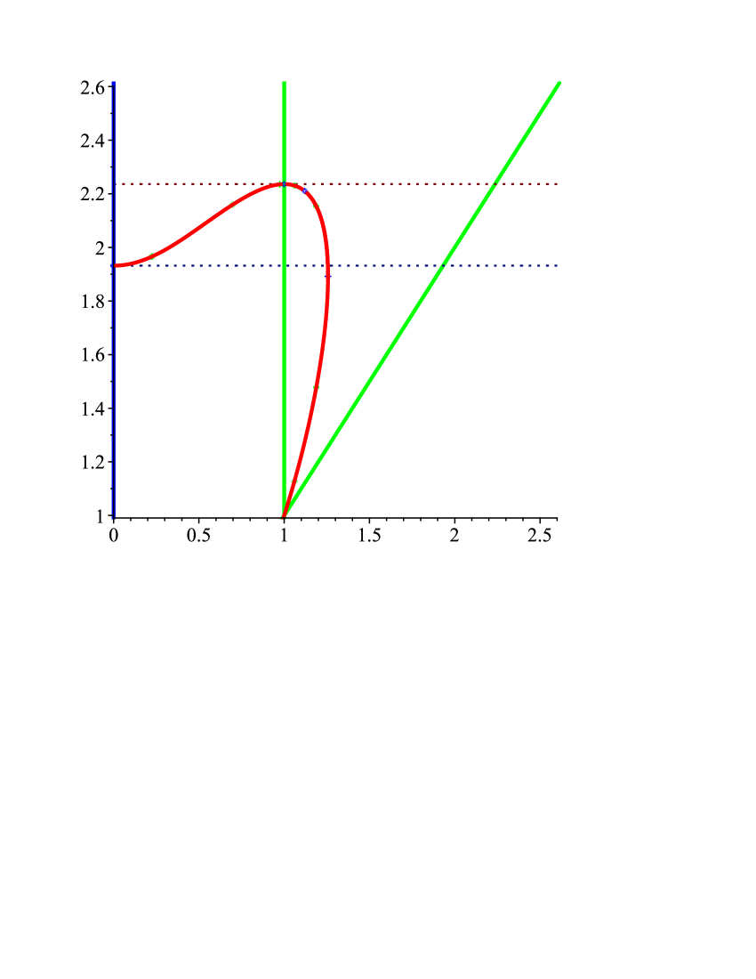
Figure 1. The zero level set of $V^{\prime}_{8}(\phi;m)$ for $\phi\geq 0$ and $m\geq 1$.

We check the criterion (1.6) for the two kinks $H_{8}\{-1,1\}$ and $H_{8}\{1,m\}$, positive results for these kinks also holds for their Lorentz boosted versions. We see that there are $2$ threshold values $k_{1}=\sqrt{2+\sqrt{3}}$ and $k_{2}=\sqrt{5}$ of the parameter $m$ (vertical axis) at which changes for the criteron (1.6) take place.

• Case $1<m\leq k_{1}$:

  • Since $\phi V^{\prime}_{8}(\phi;m)=8\phi^{2}U_{8}(\phi;m)\leq 0$ for all $\phi\in[-1,1]$, the criterion (1.6) is satisfied on $(-1,1)$ and so the kink $H_{8}\{-1,1\}$ is asymptotically stable by Theorem 2.

  • For the kink $H\{1,m\}$ the criterion is inconclusive since in the range $(1,m)$ of this kink, the function $V^{\prime}_{8}(\phi;m)$ is negative and then positive after changing sign on the red curve.

• Case $k_{1}<m<k_{2}$: the criterion is inconclusive for both kinks. Indeed, $\phi\in(-1,1)\mapsto V^{\prime}_{8}(\phi;m)$ changes sign twice while $\phi\in(1,m)\mapsto V_{8}^{\prime}(\phi;m)$ is negative and then positive.

• Case $m\geq k_{2}$:

  • For $H\{-1,1\}$ the criterion is inconclusive since $\phi\in(-1,1)\mapsto V^{\prime}_{8}(\phi;m)$ is negative and then positive.

  • Since $(\phi-1)V^{\prime}_{8}(\phi;m)\leq 0$ for any $\phi\in[1,m]$, the criterion (1.6) is satisfied on $(1,m)$ and so the kink $H\{1,m\}$ is asymptotically stable. By symmetry, the kink $H\{-m,-1\}$ is also asymptotically stable in this case.

Theorem 5 (Generalized $\phi^{8}$ model).

For the $\phi^{8}$ model with potential (5.4),

1. If $1<m\leq\sqrt{2+\sqrt{3}}$ the kink $H_{8}\{-1,1\}$ is asymptotically stable.

2. If $m\geq\sqrt{5}$ the kink $H_{8}\{1,m\}$ is asymptotically stable.

Remark 5.1.

After change of variable, the $\phi^{8}$ model considered in [55] (see also §5.5.2) corresponds to $m=3>\sqrt{5}$ and thus the kink $H_{8}\{1,3\}$ is asymptotically stable.

Remark 5.2.

There exists $\tau>0$ small such that for any $m\in(k_{1},k_{1}+\tau)$, the condition (1.6) for $V$ does not holds on $(-1,1)$, however, by Corollary 1, the kink $H\{-1,1\}$ is asymptotically stable. Indeed, setting

$$\alpha(\phi)=\frac{W_{8}(\phi;m)}{W_{8}(\phi,k_{1})}-1=\frac{(\phi^{2}-m^{2})^{2}}{(\phi^{2}-k_{1}^{2})^{2}}-1,$$

we see that for $m\in(k_{1},k_{1}+\tau)$ with $\tau>0$ small, for $k=0,1,2,3$, and any $\phi\in(-\frac{3}{2},\frac{3}{2})$,

$$|\alpha^{(k)}(\phi)|\leq C|m-k_{1}|\leq C\tau,$$

which is sufficient to apply Corollary 1.

5.3.4. The generalized $\phi^{10}$ model

The potential of the generalized $\phi^{10}$ model is

$$W_{10}(\phi;m)=\phi^{2}(\phi^{2}-1)^{2}(\phi^{2}-m^{2})^{2}$$ (5.5)

where $m>1$ is a parameter. For this model there are two types of kinks $H_{10}\{0,1\}$ and $H_{10}\{1,m\}$, and their symmetric counterparts.

The transformed potential $V_{10}$ and then $V^{\prime}_{10}$ are computed

$$V_{10}(\phi;m) =2(\phi^{2}-1)^{2}(\phi^{2}-m^{2})^{2}$$

$$\quad+4\phi^{2}\left[(\phi^{2}+1)(\phi^{2}-m^{2})^{2}+(\phi^{2}-1)^{2}(\phi^{2}+m^{2})\right]$$

$$V^{\prime}_{10}(\phi;m) =24\phi^{3}U_{10}(\phi;m),$$

where

$$U_{10}(\phi;m)=m^{4}-2\left(\phi^{2}+\frac{2}{3}\right)m^{2}+\frac{10}{3}\phi^{4}-2\phi^{2}+1.$$

We introduce

$$M_{10}^{+}(\phi)=\sqrt{\phi^{2}+\frac{2}{3}+\sqrt{-\frac{7}{3}\phi^{4}+\frac{10}{3}\phi^{2}-\frac{5}{9}}},$$

$$M_{10}^{-}(\phi)=\sqrt{\phi^{2}+\frac{2}{3}-\sqrt{-\frac{7}{3}\phi^{4}+\frac{10}{3}\phi^{2}-\frac{5}{9}}},$$

$$\mbox{for}\quad\sqrt{\frac{5}{7}-\sqrt{\frac{40}{147}}}=\phi_{1}\leq\phi\leq\phi_{2}=\sqrt{\frac{5}{7}+\sqrt{\frac{40}{147}}}.$$

As in the previous case we use Figure 2.

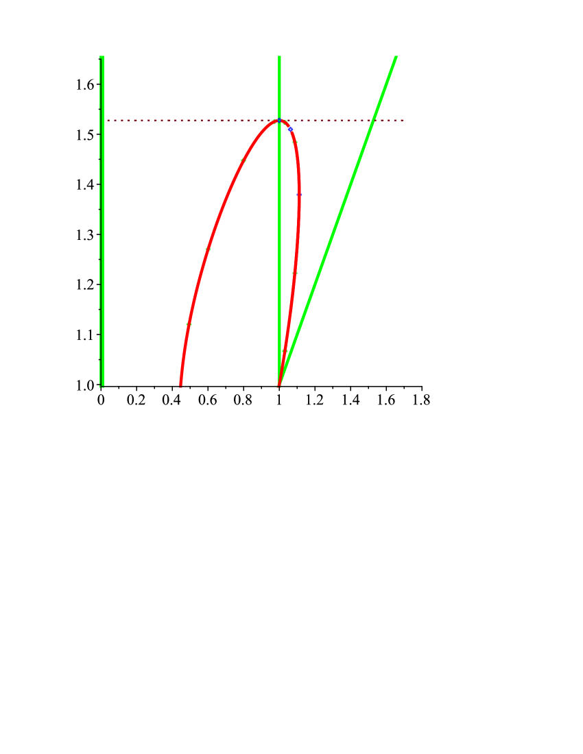
Figure 2. The zero level set of $V^{\prime}_{10}(\phi;m)$ for $\phi\geq 0$ and $m\geq 1$.

• Case $1<m<k_{1}=\frac{\sqrt{21}}{3}$:

  • On $(0,1)$, the function $\phi\mapsto V^{\prime}_{10}(\phi;m)$ is positive and then negative. The condition (1.6) holds on $(0,1)$ and so the kink $H_{10}\{0,1\}$ is asymptotically stable.

  • On $(1,m)$, the function $\phi\mapsto V^{\prime}_{10}(\phi;m)$ is negative and then positive. Thus the criterion is inconclusive for the kink $H_{10}\{1,m\}$.

• Case $m\geq k_{1}$: $V^{\prime}_{10}(\phi;m)\geq 0$ for any $\phi\geq 0$, and so both kinks $H_{10}\{0,1\}$ and $H_{10}\{1,m\}$ are asymptotically in this case stable.

Theorem 6 (Generalized $\phi^{10}$ model).

For the $\phi^{10}$ model with potential (5.5),

1. If $m>1$ then the kink $H_{10}\{0,1\}$ is asymptotically stable.

2. If $m\geq\frac{\sqrt{21}}{3}$ then the kink $H_{10}\{1,m\}$ is asymptotically stable.

Remark 5.3.

After change of variable, the $\phi^{10}$ model considered in [55] (see also §5.5.1) corresponds to $m=2>\frac{\sqrt{21}}{3}$ for which both kinks are asymptotically stable.

5.4. Maximal number of asymptotically stable kinks in the $P(\phi)_{2}$ theory

By the previous section, any kink of the generalized $\phi^{8}$ and $\phi^{10}$ models (5.5), (5.5) except the odd kink of the $\phi^{8}$ model, is asymptotically stable for $m$ large enough (see Theorems 5, 6). Now we prove a similar result for any $n\geq 2$: for $n$ wells sufficiently far away, any kink of the generalized $\phi^{4n}$ and $\phi^{4n+2}$ models, except possibly the odd kink of the $\phi^{4n}$ model, is asymptotically stable. Recall that without loss of generality, one may assume that $m_{1}=1$ (see §5.1).

Theorem 7.

There exists a sequence $(\lambda_{n})_{n}$ with $\lambda_{n}>1$ such that for any $n\geq 2$, and $(m_{1},\ldots,m_{n})$ satisfying

$$m_{j+1}\geq\lambda_{j}m_{j}>0\quad\mbox{for all $j\in\{1,\ldots,n-1\}$,}$$ (5.6)

the following hold.

1. Any kink of the $\phi^{4n}$ model with potential (5.2), except possibly the unique odd kink, is asymptotically stable.

2. Any kink of the $\phi^{4n+2}$ model with potential (5.3) is asymptotically stable.

Note that the condition on the wells is invariant by the change of variable §5.1.

Proof.

Let $W_{4n}(\phi;\mathbf{m})$ and $W_{4n+2}(\phi;\mathbf{m})$ where $\mathbf{m}=(m_{1},\dots,m_{n})$ be the potentials defined in (5.2) and (5.3). We start by proving (1). By direct computations, we have

$$V_{4n}(\phi;\mathbf{m}) =4\sum_{k=1}^{n}(\phi^{2}+m_{k}^{2})\prod_{j\neq k}^{n}(\phi^{2}-m_{j}^{2})^{2},$$ (5.7)

$$\partial_{\phi}V_{4n}(\phi;\mathbf{m}) =8\phi U_{4n}(\phi;\mathbf{m}),$$ (5.8)

where

$$U_{4n}(\phi;\mathbf{m})=\sum_{k=1}^{n}\prod_{j\neq k}^{n}(\phi^{2}-m_{j}^{2})^{2}+2\sum_{k=1,j\neq k}^{n}(\phi^{2}+m_{k}^{2})(\phi^{2}-m_{j}^{2})\prod_{l\neq k,l\neq j}^{n}(\phi^{2}-m_{l}^{2})^{2}.$$

Set

$$R_{4n}(\phi;\mathbf{m})=\sum_{k=1}^{n}\prod_{j\neq k}^{n}(\phi^{2}-m_{j}^{2})^{2}.$$ (5.9)

Note that $R_{4n}(\phi;\mathbf{m})>0$ as soon as $m_{j}<m_{j+1}$ for some $j\in\{1,\ldots,n-1\}$. We will prove the following statement by mathematical induction on $n\geq 2$: there exist constants $c_{n}$ depending only on $n$ and $\lambda_{1},\ldots,\lambda_{n-1}$ with $\lambda_{j}>1$ , such that if (5.6) holds then, for any $\phi\geq 0$

$$U_{4n}(\phi;\mathbf{m})\geq c_{n}R_{4n}(\phi;\mathbf{m}).$$ (5.10)

Suppose that this statement is true. By (5.8), it implies that $\partial_{\phi}V_{4n}(\phi;\mathbf{m})>0$ for all $\phi\in(0,\infty)$, and in particular, the condition (1.6) is satisfied for the kink connecting the wells $m_{j}$ and $m_{j+1}$, for any $j\in\{1,\ldots,n-1\}$. It also implies that $0$ is the minimum of $V_{4n}$, so condition (1.6) is not satisfied for the odd kink connecting $-m_{1}$ to $+m_{1}$.

First, we check that this property is satisfied for $n=2$. Taking $m_{1}=1$ and $m_{2}=m>1$ without loss of generality, we recall from §5.3.3

$$6U_{8}(\phi;\mathbf{m})=[6\phi^{2}-(1+m^{2})]^{2}+(m^{2}-5)(5m^{2}-1).$$

Thus, fixing any $\lambda_{1}>\sqrt{5}$ (which is consistent with (2) of Theorem 5), the property $U_{8}(\phi;\mathbf{m})\geq c_{2}\left((\phi^{2}-1)^{2}+(\phi^{2}-m^{2})^{2}\right)$ holds true for any $m\geq\lambda_{1}$, with some $c_{2}>0$ depending on the choice for $\lambda_{1}$.

Now we suppose that the property holds true up to a given $n\geq 2$ and we consider the $\phi^{4n}$ model with a configuration of wells $\mathbf{m}=(m_{1},\ldots,m_{n})$ satisfying the condition (5.6) and thus (5.10). We add another well to this model, located at $m_{n+1}=\epsilon>m_{n}$, which means that we consider the potential $W_{4(n+1)}(\phi;\mathbf{m},\epsilon)$. We check that the corresponding transformed potential writes

$$V_{4(n+1)}(\phi;\mathbf{m},\epsilon) =V_{4n}(\phi;\mathbf{m})(\phi^{2}-\epsilon^{2})^{2}+4W_{4n}(\phi;\mathbf{m})(\phi^{2}+\epsilon^{2})$$

where we have used (5.7). Differentiating with respect to $\phi$, using the notation (5.8) and the induction hypothesis, we obtain

$${2}U_{4(n+1)}(\phi;\mathbf{m},\epsilon) =(\phi^{2}-\epsilon^{2})V_{4n}(\phi;\mathbf{m})+{2}(\phi^{2}-\epsilon^{2})^{2}U_{4n}(\phi;\mathbf{m})$$

$$\quad+2W_{4n}(\phi;\mathbf{m})+(\phi^{2}+\epsilon^{2})\frac{\partial_{\phi}W_{4n}(\phi;\mathbf{m})}{\phi}$$

$$\geq 2c_{n}(\phi^{2}-\epsilon^{2})^{2}R_{4n}(\phi;\mathbf{m})+2W_{4n}(\phi;\mathbf{m})$$

$$\quad+(\phi^{2}-\epsilon^{2})V_{4n}(\phi;\mathbf{m})+(\phi^{2}+\epsilon^{2})\frac{\partial_{\phi}W_{4n}(\phi;\mathbf{m})}{\phi}.$$

For $\phi^{2}\geq\epsilon^{2}$, both terms on the second line are non-negative and since

$$R_{4(n+1)}(\phi;\mathbf{m},\epsilon)=(\phi^{2}-\epsilon^{2})R_{4n}(\phi;\mathbf{m})+W_{4n}(\phi;\mathbf{m}),$$

the property is satisfied for $\phi^{2}\geq\epsilon^{2}$.

We now restrict our attention to the case $\phi^{2}\in[0,\epsilon^{2})$. We bound

$$\frac{\partial_{\phi}W_{4n}(\phi;\mathbf{m})}{\phi}=4\sum_{k=1}^{n}(\phi^{2}-m_{k}^{2})\prod_{j\neq k}^{n}(\phi^{2}-m_{j}^{2})^{2}\geq 4(\phi^{2}-m_{n}^{2})R_{4n}(\phi;\mathbf{m})$$

and

$$V_{4n}(\phi;\mathbf{m})=4\sum_{k=1}^{n}(\phi^{2}+m_{k}^{2})\prod_{j\neq k}^{n}(\phi^{2}-m_{j}^{2})^{2}\leq 4(\phi^{2}+m_{n}^{2})R_{4n}(\phi;\mathbf{m}).$$

Therefore

$${2}U_{4(n+1)}(\phi;\mathbf{m},\epsilon)\geq\min\left(2,{c_{n}}\right)R_{4(n+1)}(\phi;\mathbf{m},\epsilon)+P_{4n}(\phi;m_{n},\epsilon)R_{4n}(\phi;\mathbf{m}),$$

where we have defined

$$P_{4n}(\phi;m_{n},\epsilon)={c_{n}}(\phi^{2}-\epsilon^{2})^{2}+4(\phi^{2}-\epsilon^{2})(\phi^{2}+m_{n}^{2})+4(\phi^{2}+\epsilon^{2})(\phi^{2}-m_{n}^{2}).$$

Expanding and completing the square gives

$$P_{4n}(\phi;m_{n},\epsilon) ={c_{n}}(\phi^{2}-\epsilon^{2})^{2}+8(\phi^{4}-\epsilon^{2}m_{n}^{2})$$

$$=(c_{n}+8)\left(\phi^{2}-\frac{c_{n}\epsilon^{2}}{c_{n}+8}\right)^{2}-\frac{c_{n}^{2}\epsilon^{4}}{c_{n}+8}+\epsilon^{4}c_{n}-8\epsilon^{2}m_{n}^{2}$$

$$\geq 8\epsilon^{4}\left(\frac{c_{n}}{c_{n}+8}-\frac{m_{n}^{2}}{\epsilon^{2}}\right).$$

Thus, if $m_{n+1}=\epsilon\geq\lambda_{n}m_{n}$ with $\lambda_{n}:=\sqrt{\frac{c_{n}+8}{c_{n}}}>1$, then

$$P_{4n}(\phi;m_{n},\epsilon)\geq 0\text{ for all }\phi\in\mathbb{R},$$

and we conclude that, with $c_{n+1}={\min(1,c_{n}/2)}$,

$$U_{4(n+1)}(\phi;\mathbf{m},\epsilon)\geq c_{n+1}R_{4(n+1)}(\phi;\mathbf{m},\epsilon).$$

To prove (2), observe that

$$V_{4n+2}(\phi;\mathbf{m})=2W_{4n}(\phi;\mathbf{m})+\phi^{2}W_{4n}(\phi;\mathbf{m})$$

and by using the explicit expression (5.7),

$$\partial_{\phi}V_{4n+2}(\phi;\mathbf{m})=8\phi^{3}\left(U_{4n}(\phi;\mathbf{m})+R_{4n}(\phi;\mathbf{m})\right),$$

which is non-negative if $\mathbf{m}$ satisfies (5.6). ∎

5.5. The $P(\phi)_{2}$ theory as approximation of the sine-Gordon theory

Following [55], we recall that the potentials $W_{4n}$ and $W_{4n+2}$ with suitable choices of wells $\{m_{k}\}_{k=1,\ldots,n}$ and after change of variables are approximations of the sine-Gordon potential for $n$ large. We study the asymptotic stability of the kinks of these models in the sine-Gordon limit.

5.5.1. The $\tilde{W}_{4n+2}$ potentials as approximation of sine-Gordon potential

Recall the formula

$$\frac{\sin(\pi\phi)}{\pi\phi}=\prod_{k=1}^{\infty}\left(1-\frac{\phi^{2}}{k^{2}}\right).$$

Thus, the sine-Gordon potential (1.8) can be written as

$$W_{\textnormal{sG}}(\phi)=1-\cos\phi=2\sin^{2}\left(\frac{\phi}{2}\right)=\frac{1}{2}\phi^{2}\prod_{k=1}^{\infty}\left(1-\frac{\phi^{2}}{(2\pi k)^{2}}\right)^{2}.$$

For $n\geq 1$, setting

$$\tilde{W}_{4n+2}(\phi)=\frac{1}{2}\phi^{2}\prod_{k=1}^{n}\left(1-\frac{\phi^{2}}{(2\pi k)^{2}}\right)^{2},$$ (5.11)

we obtain an approximation of the sine-Gordon potential, with $2n$ kinks denoted by $\tilde{H}_{4n+2}\{2\pi j,2\pi(j+1)\}$, for $j=-n,\ldots,n-1$. To study this perturbation, we use the formulation

$$\tilde{W}_{4n+2}(\phi)=\left(1-\cos\phi\right)P_{n}(\phi)\quad\mbox{where}\quad P_{n}(\phi)=\prod_{k=n+1}^{\infty}\left(1-\frac{\phi^{2}}{(2\pi k)^{2}}\right)^{-2}.$$

Then,

$$-\frac{\tilde{W}_{4n+2}^{\prime}}{\tilde{W}_{4n+2}}=-\frac{\sin\phi}{1-\cos\phi}-\frac{1}{\pi^{2}}\sum_{k=n+1}^{\infty}\frac{1}{k^{2}}\phi\left(1-\frac{\phi^{2}}{(2\pi k)^{2}}\right)^{-1}$$

and

$$\tilde{V}_{4n+2}=-\tilde{W}_{4n+2}\left(\frac{\tilde{W}_{4n+2}^{\prime}}{\tilde{W}_{4n+2}}\right)^{\prime}=P_{n}\left[1-A_{n}(1-\cos\phi)\right],$$

where

$$A_{n}=\left(\frac{P_{n}^{\prime}}{P_{n}}\right)^{\prime}=\frac{1}{\pi^{2}}\sum_{k=n+1}^{\infty}\frac{1}{k^{2}}\left(1+\frac{\phi^{2}}{(2\pi k)^{2}}\right)\left(1-\frac{\phi^{2}}{(2\pi k)^{2}}\right)^{-2}.$$

Thus,

$$\tilde{V}_{4n+2}^{\prime} =P_{n}^{\prime}\left[1-A_{n}(1-\cos\phi)\right]-P_{n}A_{n}\sin\phi-P_{n}A_{n}^{\prime}(1-\cos\phi).$$

The value of $\phi$ being fixed, for $n$ large, the following estimates hold

$$P_{n}\sim 1,\quad P_{n}^{\prime}\sim\frac{\phi}{\pi^{2}n},\quad A_{n}\sim\frac{1}{\pi^{2}n},\quad|A_{n}^{\prime}|\leq\frac{C}{n^{3}},$$

and so

$$\tilde{V}_{4n+2}^{\prime}(\phi)\sim\frac{1}{\pi^{2}n}\left(\phi-\sin\phi\right).$$

For any $J>0$, $\tilde{V}_{4n+2}^{\prime}(\phi)$ has constant sign on $(-J,0)$ and $(0,J)$, for $n$ large enough, depending on $J$. Thus, the kinks of $\tilde{W}_{4n+2}$ with range in $(-J,J)$ are asymptotically stable for such $n$.

Theorem 8 (The sine-Gordon limit for the $\phi^{4n+2}$ models).

For any $J\geq 1$, there exists $n(J)\geq 1$ such that for $n\geq n(J)$ and any $j\in\mathbb{Z}$ with $|j|\leq J$, the kink $\tilde{H}_{4n+2}\{2\pi j,2\pi(j+1)\}$ of the $\phi^{4n+2}$ model with potential (5.11) is asymptotically stable.

5.5.2. The $\tilde{W}_{4n}$ potentials as approximation of the sine-Gordon potential

Consider the shifted sine-Gordon potential $W_{{\textnormal{ssG}}}(\phi)=1-\cos(\phi+\pi)=1+\cos(\phi)$. For this model, there is an odd kink connecting $-\pi$ to $\pi$ and infinitely many other identical translated kinks. Recall

$$\cos(\pi\phi)=\frac{1}{2}\frac{\sin(2\pi\phi)}{\sin(\pi\phi)}=\prod_{k=1}^{\infty}\left(1-\frac{\phi^{2}}{(k-\tfrac{1}{2})^{2}}\right).$$

Thus, the shifted sine-Gordon potential has the infinite product expansion

$$W_{\textnormal{ssG}}=1+\cos\phi=2\cos^{2}\left(\frac{\phi}{2}\right)=2\prod_{k=1}^{\infty}\left(1-\frac{\phi^{2}}{\pi^{2}(2k-1)^{2}}\right)^{2}.$$

For $n\geq 1$, setting

$$\tilde{W}_{4n}(\phi)=2\prod_{k=1}^{n}\left(1-\frac{\phi^{2}}{\pi^{2}(2k-1)^{2}}\right)^{2},$$ (5.12)

we obtain another approximation of the sine-Gordon potential. This model has an odd kink connecting $-\pi$ to $\pi$, denoted by $\tilde{H}_{4n}\{-\pi,\pi\}$, $n-1$ positive kinks denoted by $\tilde{H}_{4n}\{\pi(2j-1),\pi(2j+1)\}$, for $j=1,\ldots,n-1$, and $n-1$ negative kinks $\tilde{H}_{4n}\{-\pi(2j+1),-\pi(2j-1)\}$. Write

$$\tilde{W}_{4n}(\phi)=\left(1+\cos\phi\right)Q_{n}(\phi)\quad\mbox{where}\quad Q_{n}(\phi)=\prod_{k=n+1}^{\infty}\left(1-\frac{\phi^{2}}{\pi^{2}(2k-1)^{2}}\right)^{-2}.$$

Then,

$$-\frac{\tilde{W}_{4n}^{\prime}}{\tilde{W}_{4n}}=\frac{\sin\phi}{1+\cos\phi}-\frac{4}{\pi^{2}}\sum_{k=n+1}^{\infty}\frac{1}{(2k-1)^{2}}\phi\left(1-\frac{\phi^{2}}{\pi^{2}(2k-1)^{2}}\right)^{-1}$$

and

$$\tilde{V}_{4n}=-\tilde{W}_{4n}\left(\frac{\tilde{W}_{4n}^{\prime}}{\tilde{W}_{4n}}\right)^{\prime}=Q_{n}\left[1-B_{n}(1+\cos\phi)\right],$$

where

$$B_{n}=\frac{4}{\pi^{2}}\sum_{k=n+1}^{\infty}\frac{1}{(2k-1)^{2}}\left(1+\frac{\phi^{2}}{\pi^{2}(2k-1)^{2}}\right)\left(1-\frac{\phi^{2}}{\pi^{2}(2k-1)^{2}}\right)^{-2}.$$

Thus,

$$\tilde{V}_{4n}^{\prime} =Q_{n}^{\prime}\left[1-B_{n}(1+\cos\phi)\right]+Q_{n}B_{n}\sin\phi-Q_{n}B_{n}^{\prime}(1+\cos\phi).$$

The value of $\phi$ being fixed, for $n$ large, the following estimates hold

$$Q_{n}\sim 1,\quad Q_{n}^{\prime}\sim\frac{\phi}{\pi^{2}n},\quad B_{n}\sim\frac{1}{\pi^{2}n},\quad|B_{n}^{\prime}|\leq\frac{C}{n^{3}},$$

and so

$$\tilde{V}_{4n}^{\prime}(\phi)\sim\frac{1}{\pi^{2}n}\left(\phi+\sin\phi\right).$$

We observe that the criterion related to the condition (1.6) is inconclusive for the odd kink $\tilde{H}_{4n}\{-\pi,\pi\}$ since on the interval $(-\pi,\pi)$ the function $\tilde{V}_{4n}^{\prime}$ is negative and then positive. For all the other kinks, the condition (1.6) holds since the sign of $\tilde{V}_{4n}^{\prime}$ is constant on $(0,\infty)$ and on $(-\infty,0)$.

Theorem 9 (The sine-Gordon limit for the $\phi^{4n}$ models).

For any $J\geq 1$, there exists $n(J)\geq 1$ such that for $n\geq n(J)$ and any $j\in\mathbb{N}$ with $1\leq j\leq J$, the kinks $\tilde{H}_{4n}\{\pi(2j-1),\pi(2j+1)\}$ and $\tilde{H}_{4n}\{-\pi(2j+1),-\pi(2j-1)\}$ of the $\phi^{4n}$ model with potential (5.12) are asymptotically stable.

5.6. The double sine-Gordon model

Last, following [9], we consider a model with infinitely many wells which is related to the sine-Gordon equation.

First, for $\eta>-\frac{1}{4}$, we consider the potential

$$W_{\textnormal{dsG}}(\phi;\eta) =\frac{4}{1+4|\eta|}\left[\eta(1-\cos\phi)+1+\cos\left(\frac{\phi}{2}\right)\right]$$ (5.13)

$$=\frac{4}{1+4|\eta|}\left[1+\cos\left(\frac{\phi}{2}\right)\right]\left[1+2\eta\left(1-\cos\left(\frac{\phi}{2}\right)\right)\right].$$

For $\eta\geq 0$, this potential interpolates between $1+\cos\left(\frac{\phi}{2}\right)$ for $\eta=0$ and $1-\cos\phi$ as $\eta\to\infty$. Since the potential is periodic of period $4\pi$, it is sufficient to check the criterion for the kink $H_{\textnormal{dsG}}$ connecting $-2\pi$ with $2\pi$. We compute

$$-\frac{W_{\textnormal{dsG}}^{\prime}}{W_{\textnormal{dsG}}}=\frac{1}{2}\frac{\sin\left(\frac{\phi}{2}\right)}{1+\cos\left(\frac{\phi}{2}\right)}-\frac{\eta\sin\left(\frac{\phi}{2}\right)}{1+2\eta\left(1-\cos\left(\frac{\phi}{2}\right)\right)},$$

and

$$V_{\textnormal{dsG}} =-W_{\textnormal{dsG}}\left(\frac{W_{\textnormal{dsG}}^{\prime}}{W_{\textnormal{dsG}}}\right)^{\prime}=\frac{1+4\eta}{1+4|\eta|}-\frac{2\eta}{1+4|\eta|}\frac{\left(1+\cos\left(\frac{\phi}{2}\right)\right)^{2}}{1+2\eta\left(1-\cos\left(\frac{\phi}{2}\right)\right)}.$$

Thus,

$$V_{\textnormal{dsG}}^{\prime}(\phi)=\frac{2\eta}{1+4|\eta|}\left(1+\cos\left(\frac{\phi}{2}\right)\right)\sin\left(\frac{\phi}{2}\right)\frac{1+3\eta-\eta\cos\left(\frac{\phi}{2}\right)}{\left[1+2\eta\left(1-\cos\left(\frac{\phi}{2}\right)\right)\right]^{2}}.$$

We see that for $-\frac{1}{4}<\eta<0$, it holds $V_{\textnormal{dsG}}^{\prime}\not\equiv 0$ and $\phi V_{\textnormal{dsG}}^{\prime}(\phi)\leq 0$ on $[-2\pi,2\pi]$, thus the kink $H_{\textnormal{dsG}}$ is asymptotically stable by Theorem 2. For $\eta>0$, the criterion is inconclusive.

Theorem 10 (Double sine-Gordon model I).

For any $-\frac{1}{4}<\eta<0$, the kink of the double sine-Gordon model with potential (5.13) is asymptotically stable.

Second, we consider the other case of double sine-Gordon models, designated as “Region I” in [9, Fig. I]. For $\eta<-\frac{1}{4}$, we set

$$W_{\textnormal{dsG}}(\phi;\eta) =\frac{4}{1+4|\eta|}\left[-\eta\cos\phi+\cos\left(\frac{\phi}{2}\right)-\eta-\frac{1}{8\eta}\right]$$ (5.14)

$$=\frac{8|\eta|}{1+4|\eta|}\left[\cos\left(\frac{\phi}{2}\right)-\frac{1}{4\eta}\right]^{2}.$$

We recall from [9] that for this potential there exist two types of kinks. Let $\zeta_{\eta}=2\arccos\frac{1}{4\eta}\in(\pi,2\pi)$. We denote by $H_{\textnormal{dsG}}\{-\zeta_{\eta},\zeta_{\eta}\}$ the odd kink connecting $-\zeta_{\eta}$ to $\zeta_{\eta}$ and by $H_{\textnormal{dsG}}\{\zeta_{\eta},4\pi-\zeta_{\eta}\}$ the kink connecting $\zeta_{\eta}$ to $4\pi-\zeta_{\eta}\in(2\pi,3\pi)$. Other kinks for this model are deduced from these two kinks by translation and symmetry. We compute

$$-\frac{W_{\textnormal{dsG}}^{\prime}}{W_{\textnormal{dsG}}}=\frac{\sin\left(\frac{\phi}{2}\right)}{\cos\left(\frac{\phi}{2}\right)-\frac{1}{4\eta}}$$

and

$$V_{\textnormal{dsG}} =-W_{\textnormal{dsG}}\left(\frac{W_{\textnormal{dsG}}^{\prime}}{W_{\textnormal{dsG}}}\right)^{\prime}=\frac{4|\eta|}{1+4|\eta|}\left[1-\frac{1}{4\eta}\cos\left(\frac{\phi}{2}\right)\right].$$

Thus,

$$V_{\textnormal{dsG}}^{\prime}=-\frac{1}{2(1+4|\eta|)}\sin\left(\frac{\phi}{2}\right).$$

For the kink $H_{\textnormal{dsG}}\{-\zeta_{\eta},\zeta_{\eta}\}$, the criterion (1.6) applies since $\phi V_{\textnormal{dsG}}^{\prime}\leq 0$ on $[-\zeta_{\eta},\zeta_{\eta}]$ and so $H_{\textnormal{dsG}}\{-\zeta_{\eta},\zeta_{\eta}\}$ is asymptotically stable from Theorem 2. For the kink $H_{\textnormal{dsG}}\{\zeta_{\eta},4\pi-\zeta_{\eta}\}$, the criterion is inconclusive since $V_{\textnormal{dsG}}^{\prime}$ is negative on $(\zeta_{\eta},2\pi)$ and positive on $(2\pi,4\pi-\zeta_{\eta})$.

Theorem 11 (Double sine-Gordon model II).

For any $\eta<-\frac{1}{4}$, the odd kink $H_{\textnormal{dsG}}\{-\zeta_{\eta},\zeta_{\eta}\}$ of the double sine-Gordon model with potential (5.14) is asymptotically stable.

Remark 5.4.

We have not considered the case $\eta=-\frac{1}{4}$ since it corresponds to a degenerate potential, not entering the general assumptions (1.3). See also (5) of Remark 2.1.

References

- [1] M.A. Alejo, C. Muñoz, and J. M. Palacios, On the variational structure of breather solutions I: Sine-Gordon equation, J. Math. Anal. Appl., 453 (2017), 1111–1138.
- [2] M.A. Alejo, C. Muñoz, and J. M. Palacios, On the asymptotic stability of the sine-Gordon kink in the energy space, preprint arXiv:2003.09358
- [3] A. Alonso-Izquierdo and J. Mateos Guilarte, On a family of (1+1)-dimensional scalar field theory models: kinks, stability, one-loop mass shifts. Ann. Physics 327 (2012), 2251–2274.
- [4] D. Bambusi, and S. Cuccagna, On dispersion of small energy solutions to the nonlinear Klein Gordon equation with a potential, Amer. J. Math., 133 (2011), 1421–1468.
- [5] E. Belendryasova and V. A. Gani, Scattering of the kinks with power-law asymptotics. Commun. Nonlinear Sci. Numer. Simul. 67 (2019), 414–426.
- [6] P. Bizoń, T. Chmaj and N. Szpak, Dynamics near the threshold for blow up in the one-dimensional focusing nonlinear Klein-Gordon equation. J. Math. Phys. 52 (2011), 103703.
- [7] V. Buslaev and G. Perelman, Scattering for the nonlinear Schrödinger equations: states close to a soliton, St.Petersburgh Math. J., 4 (1993), 1111–1142.
- [8] V. Buslaev and G. Perelman, On the stability of solitary waves for nonlinear Schrödinger equations, Nonlinear evolution equations, Amer. Math. Soc. Transl. Ser. 2, 164 (1995), 75–98.
- [9] D. Campbell, M. Peyrard, and P. Sodano, Kink-antikink interactions in the double sine-Gordon equation, Physica D, 19 (1986), 165–205.
- [10] S.-M. Chang, S. Gustafson, K. Nakanishi and T.-P. Tsai, Spectra of linearized operators for NLS solitary waves, SIAM J. Math. Anal. 39 (2007/08), 1070–1111.
- [11] R. Côte, C. Muñoz, D. Pilod, and G. Simpson, Asymptotic Stability of high-dimensional Zakharov-Kuznetsov solitons, Arch. Rat. Mech. Anal., 220 (2016), 639–710.
- [12] S. Cuccagna, On asymptotic stability in 3D of kinks for the model, Trans. Amer. Math. Soc., 360 (2008), 2581–2614.
- [13] S. Cuccagna, The Hamiltonian structure of the nonlinear Schrödinger equation and the asymptotic stability of its ground states, Comm. Math. Phys., 305 (2011), 279–331.
- [14] S. Cuccagna, On asymptotic stability of moving ground states of the nonlinear Schrödinger equation, Trans. Amer. Math. Soc., 366 (2014), 2827–2888.
- [15] S. Cuccagna and M. Maeda, On stability of small solitons of the 1-D NLS with a trapping delta potential, preprint arXiv:1904:11869
- [16] S. Cuccagna and D. Pelinovsky, The asymptotic stability of solitons in the cubic NLS equation on the line, Applicable Analysis, 93 (2014), 791–822.
- [17] S. Cuenda, N. R. Quintero and A. Sánchez, Sine-Gordon wobbles through Bäcklund transformations, Discrete and Continuous Dynamical Systems - Series S, 4 (2011), 1047–1056.
- [18] T. Dauxois, and M. Peyrard, Physics of solitons, Cambridge University Press, Cambridge, 2010. xii+422 pp.
- [19] J.-M. Delort, Existence globale et comportement asymptotique pour l’équation de Klein-Gordon quasi linéaire à données petites en dimension 1, Ann. Sci. École Norm. Sup., 34(4) (2001), 1–61.
- [20] J.-M. Delort, Semiclassical microlocal normal forms and global solutions of modified one-dimensional KG equations, Annales de l’Institut Fourier, 66 (2016) 1451–1528.
- [21] J.-M. Delort, Modified scattering for odd solutions of cubic nonlinear Schrödinger equations with potential in dimension one. Preprint hal-01396705, version 1 (2016).
- [22] J.-M. Delort, D. Fang, and R. Xue, Global existence of small solutions for quadratic quasilinear Klein-Gordon systems in two space dimensions, J. Funct. Anal., 211 (2004), 288–323.
- [23] J.-M. Delort and N. Masmoudi, Long time dispersive estimates for perturbations of a kink solution of one dimensional cubic wave equations. Preprint 2020. hal-02862414.
- [24] J. Denzler, Nonpersistence of breather families for the perturbed sine-Gordon equation, Comm. Math. Phys., 158 (1993), 397–430.
- [25] G. Fibich, F. Merle and P. Raphaël, Proof of a Spectral Property related to the singularity formation for the critical nonlinear Schrödinger equation, Physica D, 220 (2006), 1–13.
- [26] V. A. Gani, V. Lensky, and M. A. Lizunova, Kink excitation spectra in the (1+1)-dimensional model, JHEP, 147 (2015).
- [27] P. Germain and F. Pusateri, Quadratic Klein-Gordon equations with a potential in one dimension. Preprint arXiv:2006.15688
- [28] P. Germain, F. Pusateri and F. Rousset, Asymptotic stability of solitons for mKdV, Advances in Mathematics, 299(2016), 272–330.
- [29] Gol’dman, I. I. and Krivchenkov, V. D. and Geĭlikman, B. T. and Marquit, E. and Lepa, E., Problems in quantum mechanics, Authorised revised ed. Edited by B. T. Geilikman; translated from the Russian by E. Marquit and E. Lepa, Pergamon Press, 1961.
- [30] N. Hayashi and P. Naumkin, The initial value problem for the cubic nonlinear Klein-Gordon equation, Z. Angew. Math. Phys., 59 (2008), 1002–1028.
- [31] N. Hayashi and P. Naumkin, Quadratic nonlinear Klein-Gordon equation in one dimension, J. Math. Phys., 53 (2012), 103711.
- [32] D. B. Henry, J. F. Perez, and W. F. Wreszinski, Stability theory for solitary-wave solutions of scalar field equations, Comm. Math. Phys. 85 (1982), no. 3, 351–361.
- [33] H. Ito and H. Tasaki, Stability theory for nonlinear Klein-Gordon kinks and Morse’s index theorem, Phys. Lett. A 113 (1985), 179–182.
- [34] J. Jendrej, M. Kowalczyk and A. Lawrie, Dynamics of strongly interacting kink-antikink pairs for scalar fields on a line, preprint arXiv:1911.02064
- [35] P. G. Kevrekidis and J. Cuevas-Maraver, A Dynamical Perspective on the Model. Past, Present and Future. Nonlinear Systems and Complexity Series. Springer 2019.
- [36] A. Khare, I. C. Christov, and A. Saxena, Successive phase transitions and kink solutions in , and field theories, Phys. Rev. E 90, 023208 – Published 27 August 2014.
- [37] S. Klainerman, Global existence for nonlinear wave equations, Comm. Pure Appl. Math. 33 (1980), pp. 43–101.
- [38] S. Klainerman, Global existence of small amplitude solutions to nonlinear Klein-Gordon equations in four space-time dimensions, Comm. Pure Appl. Math., 38 (1985), 631–641.
- [39] E. Kopylova and A. I. Komech, On asymptotic stability of kink for relativistic Ginzburg-Landau equations, Arch. Ration. Mech. Anal., 202 (2011), 213–245.
- [40] E. Kopylova and A. I. Komech, On asymptotic stability of moving kink for relativistic Ginzburg-Landau equation, Comm. Math. Phys., 302 (2011), 225–252.
- [41] M. Kowalczyk, Y. Martel, and C. Muñoz, Kink dynamics in the model: asymptotic stability for odd perturbations in the energy space, J. Amer. Math. Soc., 30 (2017), 769–798.
- [42] M. Kowalczyk, Y. Martel, and C. Muñoz, Nonexistence of small, odd breathers for a class of nonlinear wave equations, Letters in Mathematical Physics, 107 (2017), 921–931.
- [43] M. Kowalczyk, Y. Martel, and C. Muñoz, On asymptotic stability of nonlinear waves, Séminaire Laurent Schwartz - Équations aux dérivées partielles et applications. Année 2016-2017. Ed. Éc. Polytechnique Palaiseau, 2017, Exp. No. XVIII.
- [44] M. Kowalczyk, Y. Martel, and C. Muñoz, Soliton dynamics for the 1D NLKG equation with symmetry and in the absence of internal modes. To appear in Journal of European Mathematical Society.
- [45] J. Krieger and W. Schlag, Stable manifolds for all monic supercritical focusing nonlinear Schrödinger equations in one dimension, J. Amer. Math. Soc. 19 (2006), 815-920.
- [46] J. Krieger, K. Nakanishi and W. Schlag, Global dynamics above the ground state energy for the one-dimensional NLKG equation, Math. Z. 272 (2012), no. 1-2, 297-316.
- [47] M.D Kruskal and H. Segur, Nonexistence of small-amplitude breather solutions in theory, Phys. Rev. Lett., 58 (1987), 747–750.
- [48] G.L. Lamb, Elements of Soliton Theory, Pure Appl. Math., Wiley, New York (1980).
- [49] H. Lindblad, J. Lührmann and A. Soffer, Decay and asymptotics for the 1D Klein-Gordon equation with variable coefficient cubic nonlinearities, preprint arXiv:1907.09922
- [50] H. Lindblad, J. Lührmann and A. Soffer, Asymptotics for 1D Klein-Gordon equations with variable coefficient quadratic nonlinearities, preprint arXiv:2006.00938
- [51] H. Lindblad and A. Soffer, A remark on long range scattering for the nonlinear Klein-Gordon equation, J. Hyperbolic Differ. Equ., 2 (2005), 77–89.
- [52] H. Lindblad and A. Soffer, A remark on asymptotic completeness for the critical nonlinear Klein-Gordon equation, Lett. Math. Phys., 73 (2005), 249–258.
- [53] H. Lindblad and A. Soffer, Scattering for the Klein-Gordon equation with quadratic and variable coefficient cubic nonlinearities, Trans. Amer. Math. Soc., 367 (2015), 8861–8909.
- [54] H. Lindblad and T. Tao. Asymptotic decay for a one-dimensional nonlinear wave equation, Anal. PDE, 5 (2012), 411-422.
- [55] M. A. Lohe, Soliton structures in , Physical Review D, 20 (1979), 3120–3130.
- [56] N. S. Manton and P. Sutcliffe, Topological solitons, Cambridge Monographs on Mathematical Physics, Cambridge University Press, Cambridge (2004).
- [57] Y. Martel, Linear problems related to asymptotic stability of solitons of the generalized KdV equations, SIAM J. Math. Anal. 38 (2006), 759-781.
- [58] Y. Martel, and F. Merle, Liouville theorem for the critical generalized Korteweg-de Vries equation, J. Math. Pures Appl., 79 (2000), 339–425.
- [59] Y. Martel, and F. Merle, Asymptotic stability of solitons for subcritical generalized KdV equations, Arch. Ration. Mech. Anal., 157 (2001),219–254.
- [60] Y. Martel, and F. Merle, Asymptotic stability of solitons of the gKdV equations with general nonlinearity, Math. Ann. 341 (2008), 391–427.
- [61] F. Merle and P. Raphaël, The blow-up dynamic and upper bound on the blow-up rate for critical nonlinear Schrödinger equation, Ann. of Math. (2), 161 (2005), 157–222.
- [62] C. Muñoz, and J. M. Palacios, Nonlinear stability of 2-solitons of the Sine-Gordon equation in the energy space, Ann. Inst. H. Poincaré, Anal. Non Linéaire, 36 (2019), 977–1034.
- [63] R.L. Pego and M.I. Weinstein, Asymptotic stability of solitary waves. Comm. Math. Phys. 164 (1994), 305-349.
- [64] M. E. Peskin and D. V. Schroeder, An introduction to quantum field theory, Addison-Wesley Publishing Company, Advanced Book Program, Reading, MA. (1995).
- [65] P. Raphaël and I. Rodnianski, Stable blow up dynamics for the critical co-rotational wave maps and equivariant Yang-Mills problems, Publ. Math. Inst. Hautes Études Sci. 115 (2012), 1-122.
- [66] M. Reed and B. Simon, Analysis of Operators IV. Methods of Modern Mathematical Physics. Academic Press, 1978.
- [67] W. Schlag, Spectral theory and nonlinear partial differential equations: a survey, Discrete Contin. Dyn. Syst. 15 (2006), no. 3, 703–723.
- [68] W. Schlag, Dispersive estimates for Schrödinger operators: A survey, Mathematical aspects of nonlinear dispersive equations, 255–285, Ann. of Math. Stud., 163, Princeton Univ. Press, Princeton, NJ, 2007.
- [69] H. Segur, Wobbling kinks in and sine-Gordon theory, J. Math. Phys., 24 (1983), 1439–1443.
- [70] J. Shatah, Normal forms and quadratic Klein-Gordon equations, Comm. Pure Applied Math., 33 (1985), 685–696.
- [71] A. Soffer and M. I. Weinstein, Time dependent resonance theory, Geom. Funct. Anal. 8 (1998), 1086–1128.
- [72] A. Soffer and M. I. Weinstein, Resonances, radiation damping and instability in Hamiltonian nonlinear wave equations, Invent. Math. 136 (1999), 9–74.
- [73] J. Sterbenz, Dispersive Decay for the 1D Klein-Gordon Equation with Variable Coefficient Nonlinearities, Trans. Amer. Math. Soc., 368 (2016), 2081–2113.
- [74] T. Vachaspati, Kinks and domain walls, Cambridge University Press, New York (2006).
- [75] A. Vilenkin and E. P. S. Shellard, Cosmic strings and other topological defects, Cambridge Monographs on Mathematical Physics, Cambridge University Press, Cambridge (1994).
- [76] M. I. Weinstein, Modulational stability of ground states of nonlinear Schrödinger equations, SIAM J. Math. Anal., 16 (1985), 472–491.
- [77] E. Witten, From superconductors and four-manifolds to weak interactions, Bull. Amer. Math. Soc., 44 (2007), 361–391.
- [78] D. Wei and S. Yang, Asymptotic decay for defocusing semilinear wave equations in , preprint arXiv:2003.12264
- [79] P. E. Zhidkov, On the existence of the solution of the Cauchy problem and the stability of kink solutions of the nonlinear Schrödinger equation. (Russian) Sibirsk. Mat. Zh. 33 (1992), 73–-9, 220; translation in Siberian Math. J. 33 (1992), 239–246.