Multiplicative noise and the diffusion of conserved densities

Abstract

Stochastic fluid dynamics governs the long time tails of hydrodynamic correlation functions, and the critical slowing down of relaxation phenomena in the vicinity of a critical point in the phase diagram. In this work we study the role of multiplicative noise in stochastic fluid dynamics. Multiplicative noise arises from the dependence of transport coefficients, such as the diffusion constants for charge and momentum, on fluctuating hydrodynamic variables. We study long time tails and relaxation in the diffusion of a conserved density (model B), and a conserved density coupled to the transverse momentum density (model H). Careful attention is paid to fluctuation-dissipation relations. We observe that multiplicative noise contributes at the same order as non-linear interactions in model B, but is a higher order correction to the relaxation of a scalar density and the tail of the stress tensor correlation function in model H.

1 Introduction

There is a very successful description of heavy ion collisions at the Relativistic Heavy Ion Collider (RHIC) and the Large Hadron Collider (LHC) based on relativistic fluid dynamics Romatschke and Romatschke [2019], Jeon and Heinz [2015], Teaney [2010]. Up-to-date models include higher order gradient corrections to the relativistic Navier-Stokes theory, kinetic theory afterburners, and initial state models that account for event-by-event fluctuations.

Recently, a number of authors have reexamined the role of fluctuations in relativistic and non-relativistic fluid dynamics De Schepper et al. [1974], Pomeau and Resibois [1975], Kovtun and Yaffe [2003], Peralta-Ramos and Calzetta [2012], Kovtun et al. [2011], Kapusta et al. [2012], Kovtun [2012], Chafin and Schäfer [2013], Akamatsu et al. [2017], Martinez and Schäfer [2019], Chen-Lin et al. [2019], Akamatsu et al. [2019], An et al. [2019]. Fluctuations arise from the fact that fluid dynamics is a coarse-grained description, and that the macroscopic variables arise from averaging over unresolved degrees of freedom at some resolution scale $l$. In approximate local thermal equilibrium these microscopic degrees of freedom exhibit thermal fluctuations that scale as $l^{-d/2}$, where the $d$ is the number of spatial dimensions. As the resolution scale becomes finer, the relative importance of fluctuations becomes larger. Fluid dynamics is a non-linear theory, and the couplings between hydrodynamic modes lead to novel effects that go beyond Gaussian noise in the macroscopic variables. A well-known example is the emergence of hydrodynamic "tails", non-analytic terms in the frequency or time-dependence of correlation functions.

In this paper we will address a specific aspect of hydrodynamic fluctuations, the role of non-linear or “multiplicative” noise. Non-linear noise terms arise naturally in applications of fluid dynamics to relativistic heavy ion collisions. Fluctuation-dissipation relations imply that the strength of noise terms is governed by dissipative coefficients, such as diffusion constants and viscosities. These coefficients are themselves functions of fluctuating hydrodynamic variables, such as the entropy and baryon density of the fluid. As a consequence, noise terms are necessarily non-linear.

There are a number of questions that immediately arise. The first is how multiplicative noise fits into the power counting governed by the low energy (gradient) expansion. Naively, non-linear terms in the noise are not suppressed by extra gradients, so they might modify leading order predictions for the non-analyticities in correlation functions, or for the scaling behavior in the vicinity of a critical point. A second problem is to determine the precise form of the fluctuation-dissipation (FD) relation in the presence of multiplicative noise. This problem has been studied in the past Wang and Heinz [2002], but the FD relations have not been checked in specific hydrodynamics theories of multiplicative noise. We also note that there is a substantial body of literature on stochastic equations with multiplicative noise Habib [1993], Arnold [2000a, b], Aron et al. [2010], Arenas and Barci [2012], Biro and Jakovac [2005].

In this work we focus on the effect of multiplicative noise on the low energy expansion of hydrodynamic correlation functions. This paper is structured as follows: In Section 2 we introduce an effective theory of non-linear diffusion with multiplicative noise. In Section 3 we formulate and check the FD relation, and compute corrections to the two-point function of the conserved density. In Section 4-6 we extend this analysis to the theory of a conserved density interacting with transverse shear waves (model H in the classification of Hohenberg and Halperin Hohenberg and Halperin [1977]). We compute both the density and momentum density correlation functions, related to the relaxation rate and the renormalization of the shear viscosity.

2 Diffusion

In this Section we study the diffusion of a conserved density $\psi(x,t)$. The diffusion equation is given by

$$\partial_{t}\psi(x,t)=\vec{\nabla}\left\{\kappa(\psi)\,\vec{\nabla}\,\left(\frac{\delta{\cal F}[\psi]}{\delta\psi}\right)\right\}+\theta(x,t)\,,$$ (1)

where $\kappa(\psi)$ is a density dependent conductivity, ${\cal F}[\psi]$ is a free energy functional, and $\theta(x,t)$ is a noise term. Equ. (1) is the diffusion equation of model B, modified by a field dependent conductivity $\kappa(\psi)$. In the following we will write

$$\kappa(\psi)=\kappa_{0}\left(1+\lambda_{D}\psi\right)\,,$$ (2)

and we will use a free energy functional of the form

$${\cal F}[\psi]=\int d^{3}x\,\left\{\frac{1}{2}(\vec{\nabla}\psi)^{2}+\frac{r}{2}\,\psi(x,t)^{2}+\frac{\lambda}{3!}\,\psi(x,t)^{3}+h(x,t)\psi(x,t)\right\}\,,$$ (3)

where $h(x,t)$ is an external field. Higher order terms in $\kappa(\psi)$ and ${\cal F}[\psi]$ can be taken into account, but do not change our conclusions. The noise term $\theta(x,t)$ is Gaussian, with a distribution

$$P[\theta]\sim\exp\left(-\frac{1}{4}\int d^{3}x\,dt\,\theta(x,t)L(\psi)^{-1}\theta(x,t)\right)\,,$$ (4)

where $L$ is a noise kernel that we will specify below. Correlation functions of this theory are computed from solutions of the diffusion equation, averaged over the noise distribution in equ. (4). Martin, Siggia, Rose, as well as Janssen and de Dominicis (MSRJD), showed how to write this noise average in terms of a stochastic field theory Martin et al. [1973], Janssen [1976], De Dominicis and Peliti [1978]. This theory contains the hydrodynamic variable $\psi(x,t)$ as well as an auxiliary field $\tilde{\psi}(x,t)$. The partition function is

$$Z=\int{\cal D}\psi\,{\cal D}\tilde{\psi}\;\exp\left(-\int d^{3}x\,dt\,{\cal L}(\psi,\tilde{\psi})\right)\,.$$ (5)

The effective Lagrangian of this theory is

$${\cal L}(\psi,\tilde{\psi})=\tilde{\psi}\left(\partial_{t}-D_{0}\nabla^{2}\right)\psi-\frac{D_{0}\lambda^{\prime}}{2}\left(\nabla^{2}\tilde{\psi}\right)\psi^{2}-\tilde{\psi}L(\psi)\tilde{\psi}\,,$$ (6)

where we have defined the diffusion constant $D_{0}=r\kappa_{0}$ and $\lambda^{\prime}=\lambda/r+\lambda_{D}$. We have dropped an $O(\nabla^{4})$ term in the quadratic part of the Lagrangian, which is important in the vicinity of a critical point when $r\to 0$. Note that in deriving this Lagrangian we have dropped a Jacobian that can be written in terms of a set of ghost fields. As explained in Täuber [2014], Kovtun [2012] ghost loops cancel pure vacuum diagrams that arise in the perturbative expansion. In the following we do not explicitly write down ghost propagators and vertices, and simply drop pure vacuum diagrams.

An important observation is that for a suitable choice of the noise kernel $L(\psi)$ the effective Lagrangian enjoys a time reversal symmetry Bausch et al. [1976], Janssen [1979]. In the following we will choose

$$L(\psi)=\reflectbox{$\vec{\reflectbox{$\nabla$}}$}\left[k_{B}T\kappa(\psi)\right]\vec{\nabla}\,.$$ (7)

We will also employ units such that $k_{B}T=1$. We define the $\mathcal{T}$-reversal of the stochastic fields as

$$\mathcal{T}\psi(t) = \psi(-t),$$ (8)

$$\mathcal{T}\tilde{\psi}(t) = -\left(\tilde{\psi}(-t)-\frac{\delta{\cal F}[\psi(-t),\tilde{\psi}(-t)]}{\delta\psi(-t)}\right)\,.$$ (9)

Under $\mathcal{T}$ the Lagrangian transforms as

$$\mathcal{T}{\cal L}(\psi(t),\tilde{\psi}(t))={\cal L}(\psi(-t),\tilde{\psi}(-t))-\frac{d}{dt}\,{\cal F}[\psi(-t),\tilde{\psi}(-t)]\,.$$ (10)

The total derivative term implies the detailed balance condition

$$\exp\left(-\left[S(T_{1},T_{2})-S(-T_{1},-T_{2})\right]\right)=\exp\left(-\Delta{\cal F}\right)\,,$$ (11)

where

$$S(T_{1},T_{2})=\int_{T_{1}}^{T_{2}}dt\,d^{3}x\,{\cal L}(\psi,\tilde{\psi})\,,$$ (12)

and $\Delta{\cal F}={\cal F}[\psi(T_{2}),\tilde{\psi}(T_{2})]-{\cal F}[\psi(T_{1}),\tilde{\psi}(T_{1})]$. The $\mathcal{T}$ invariance of the MSRJD effective action was first studied in Janssen [1979], for the case of a density-independent diffusion constant. We have verified that the symmetry continues to hold in the density dependent case, provided we use the symmetric noise kernel in equ. (7). We note that the $T$-reversal symmetry in equ. (8,9) is closely related to the dynamical KMS-symmetry studied in Crossley et al. [2017], Glorioso et al. [2017], Chen-Lin et al. [2019].

Time reversal invariance can be used to derive fluctuation-dissipation relations. For this purpose we define the response function as the derivative of $\langle\psi(t)\rangle_{h}$ with respect to the external field in equ. (3). The response function is given by

$$G_{R}(x,t;x^{\prime},t^{\prime})=\left.\frac{\delta\langle\psi(x,t)\rangle}{\delta h(x^{\prime},t^{\prime})}\right|_{h=0}\,.$$ (13)

As explained in the appendix we can show that the response function is related to the correlation function

$$\left\langle\psi(x_{1},t_{1})\left[\reflectbox{$\vec{\reflectbox{$\nabla$}}$}\kappa(\psi)\vec{\nabla}\tilde{\psi}\right](x_{2},t_{2})\right\rangle=\Theta(t_{2}-t_{1})\left\langle\psi(x_{1},t_{1})\dot{\psi}(x_{2},t_{2})\right\rangle\,.$$ (14)

This relation generalizes to higher order $n$-point functions. The response of the $(n-1)$-point function is related to time-ordered $n$-point function. In momentum space equ. (14) is equivalent to

$$2\,{\rm Im}\;\left\{k^{2}\left\langle\psi(\omega,k)[\kappa(\psi)\tilde{\psi}](-\omega,-k)\right\rangle\right\}=\omega\left\langle\psi(\omega,k)\psi(-\omega,-k)\right\rangle\,.$$ (15)

This is the standard FD relation in the case $\kappa(\psi)=\kappa_{0}$, but for a field dependent diffusion constant the left hand side of equ. (15) includes the vertex function of the composite operator $[\kappa(\psi)\tilde{\psi}]$.

3 Response and correlation functions

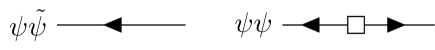
(a)

(b)

(c)

Figure 1: Feynman rules of the diffusive field theory (model B). The vertex denoted by the solid circle is a non-linear interaction term, and the vertex denoted by a solid square is a new interaction generated by the field dependence of the diffusion constant.

In this Section we will compute the response and correlation functions of the purely diffusive theory at leading order in low frequency, low momentum expansion. For this purpose we split the effective Lagrangian into a quadratic and an interaction part. The quadratic part of the action generates a matrix propagator in the $(\psi,\tilde{\psi})$ basis. The off-diagonal matrix elements are retarded/advanced functions

$$G_{0}(\omega,k)=\langle\tilde{\psi}\psi\rangle_{\omega,k}=\langle\psi\tilde{\psi}\rangle_{-\omega,k}=\frac{1}{-i\omega+D_{0}k^{2}}\,,$$ (16)

and the diagonal components are the correlation function

$$C_{0}(\omega,k)=\langle\psi\psi\rangle_{\omega,k}=\frac{2\kappa_{0}k^{2}}{\omega^{2}+(D_{0}k^{2})^{2}}\,,$$ (17)

as well as $\langle\tilde{\psi}\tilde{\psi}\rangle_{\omega,k}=0$. The interaction term is

$${\cal L}_{\it int}=-\frac{D_{0}\lambda^{\prime}}{2}\left(\nabla^{2}\tilde{\psi}\right)\psi^{2}-\frac{D_{0}\lambda_{D}}{r}\left(\vec{\nabla}\tilde{\psi}\right)^{2}\psi\,,$$ (18)

and the corresponding vertices are shown in Fig. 1, where we have set $r=1$. We observe that both interaction terms involve two derivatives, and we expect the non-linear interaction and the field dependent diffusion constant to contribute at the same order in the low energy expansion. However, the field dependent diffusion constant leads to a new type of vertex not present in the standard MSRJD effective action. This type of vertex was previously obtained in Chen-Lin et al. [2019], based on diffeomorphism invariance of the effective action on the Keldysh contour.

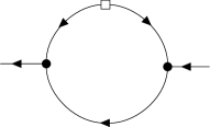
(a)

(b)

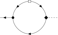
(c)

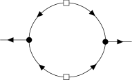
(d)

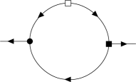
(e)

Figure 2: One-loop contributions to the response function (a)-(c) and the correlation function (d)-(e) in model B. Diagram (a) contains only the non-linear interaction, whereas diagram (b) also depends a new vertex generated by the field dependent diffusion constant. Diagram (c) is a new type of diagram that contains the composite operator $\lambda_{D}[\psi\vec{\nabla}\tilde{\psi}]$. Diagrams (d,e) are the corresponding corrections to the correlation function.

One-loop corrections to the retarded and symmetric correlation are shown in Fig. 2. Diagrams (a,b) are self energy corrections to the retarded correlation functions. The self energy modifies the retarded function as

$$G(\omega,k)=\frac{1}{-i\omega+D_{0}k^{2}+\Sigma(\omega,k)}\,.$$ (19)

At one-loop order, we find

$$\Sigma(\omega,k)=\frac{\lambda^{\prime}}{32\pi}\left(i\lambda^{\prime}\omega k^{2}+\lambda_{D}\left[i\omega-D_{0}k^{2}\right]k^{2}\right)\sqrt{k^{2}-\frac{2i\omega}{D_{0}}}\,.$$ (20)

Here, we have regularized the loop integral and dropped cutoff-dependent terms that can be absorbed into the bare diffusion constant. The result in equ. (20) shows that $\lambda_{D}$ indeed contributes at the same order as ordinary non-linear interactions. We note, however, that the functional form of the correction is different, so that it is possible to disentangle the corrections from $\lambda^{\prime}$ and $\lambda_{D}$. Finally, we note that in the limit $k^{2}\to 0$ the coefficient of the self energy is shifted $\lambda^{\prime 2}\to\lambda^{\prime}(\lambda^{\prime}+\lambda_{D})$, indicating that the density dependence of $D_{0}$ corrects the long-time tail of the response function by an overall factor $(1+\lambda_{D}/\lambda^{\prime})$.

Diagrams (d,e) provide corrections to the correlation function, which is modified as

$$C(\omega,k)=\frac{2D_{0}k^{2}+\delta D(\omega,k)}{\left(-i\omega+D_{0}k^{2}+\Sigma(\omega,k)\right)\left(i\omega+D_{0}k^{2}+\Sigma(-\omega,k)\right)}\,,$$ (21)

where

$$\delta D(\omega,k)=\frac{D_{0}\lambda^{\prime}}{16\pi}\left(\lambda^{\prime}+2\lambda_{D}\right)k^{4}\;{\mathrm{Re}}\,\,\sqrt{k^{2}-\frac{2i\omega}{D_{0}}}\,.$$ (22)

Diagram (c) shows the one-loop contribution with one insertion of the composite operator $\lambda_{D}[\psi\vec{\nabla}\tilde{\psi}]$. We define the corresponding vertex function by

$$\Gamma_{D}(\omega,k)\equiv(-i\omega+D_{0}k^{2})\left\langle D_{0}\lambda_{D}[\psi\vec{\nabla}\tilde{\psi}]\vec{\nabla}\psi\right\rangle_{\omega,k}$$ (23)

and get

$$\Gamma_{D}(\omega,k)=\frac{D_{0}\lambda^{\prime}\lambda_{D}}{32\pi}\,k^{4}\,\sqrt{k^{2}-\frac{2i\omega}{D_{0}}}\,.$$ (24)

We can now verify the fluctuation-dissipation relation. In terms of the Green and vertex functions defined in this Section the FD relation in equ. (15) becomes

$$2\,{\mathrm{Im}}\,\left\{G(\omega,k)\left[D_{0}k^{2}+\Gamma_{D}(\omega,k)\right]\right\}=\omega C(\omega,k)\,.$$ (25)

Using equ. (19-24) we observe that this relation is indeed satisfied. In the limit $\lambda_{D}=0$ (no multiplicative noise) equ. (25) reduces to the well known relation between the retarded function and the correlation function. However, in the presence of multiplicative noise the contribution of the vertex function $\Gamma_{D}$ is essential in satisfying the FD relation.

4 Shear modes and model H

In this Section we will extend our result to a conserved density $\psi$ that is advected by the momentum density $\vec{\pi}$ of a fluid. This theory is known as model H Hohenberg and Halperin [1977], and describes the critical behavior of a fluid near the liquid-gas endpoint. In the following we will assume that the fluid is approximately incompressible, $\nabla_{k}\pi_{k}\simeq 0$. This implies that we are only taking into account the coupling to shear modes, neglecting the role of sound. This approximation is sufficient to capture the critical dynamics in model H, and to compute the shear contribution to hydrodynamic tails.

(a)

(b)

(c)

(d)

(e)

Figure 3: Feynman rules for model H, describing the interaction of the transverse momentum density $\pi_{k}$ with a scalar density $\psi$. The vertex denoted by the solid circle is a non-linear interaction term, and the vertex denoted by a solid square is a new interaction generated by the field dependence of the diffusion constant. Note: $P_{abij}=\delta_{ab}\delta_{ij}$.

In the presence of a conserved momentum density the diffusion equation contains a new coupling, $\partial_{t}\psi(x,t)\sim w^{-1}\pi_{k}\nabla_{k}\psi(x,t)$, where $w$ is the enthalpy density of the fluid. In order to obtain the correct equilibrium distribution in the presence of this coupling it is important to note that this interaction derives from a Poisson bracket Dzyaloshinskii and Volovick [1980]

$$\partial_{t}\psi(x,t)=\ldots-\int d^{3}x^{\prime}\,\left\{\psi(x,t),\pi_{k}(x^{\prime},t\right\}\frac{\delta\mathcal{F}[\psi,\pi_{l}]}{\delta\pi_{k}}=\ldots-\frac{1}{w}\pi_{k}\nabla_{k}\psi(x,t)\,,$$ (26)

where $\ldots$ denotes the right hand side of equ. (1) and the free energy density is

$$\mathcal{F}[\psi,\pi_{k}]=\mathcal{F}[\psi]+\int d^{3}x\,\left\{\frac{1}{2w}\,\vec{\pi}^{2}+\pi_{k}{\cal A}_{k}\right\}\,,$$ (27)

where $\mathcal{F}[\psi]$ is defined in equ. (3) and ${\cal A}_{k}$ is an external field coupled to the momentum density. Note that in a fully covariant formalism ${\cal A}_{k}$ corresponds to the $g_{0k}$ components of the metric tensor. The equation of motion for the momentum density is

$$\partial_{t}\pi_{i}(x,t)=\vec{\nabla}\left\{\eta(\psi)\,\vec{\nabla}\,\left(\frac{\delta{\cal F}[\psi,\pi_{k}]}{\delta\pi_{i}}\right)\right\}+\frac{\delta\mathcal{F}[\psi,\pi_{k}]}{\delta\psi}\nabla_{i}\psi-\frac{\delta\mathcal{F}[\psi,\pi_{l}]}{\delta\pi_{k}}\nabla_{k}\pi_{i}+\xi_{i}(x,t)\,,$$ (28)

where we have neglected terms proportional to $\nabla_{k}\pi_{k}$ and $\xi_{i}$ is a stochastic force. The stochastic force has a Gaussian probability distribution

$$P[\xi_{i}]\sim\exp\left(-\frac{1}{4}\int d^{3}x\,dt\,\xi_{i}(x,t)\left[M(\psi)^{-1}\right]_{ij}\xi_{j}(x,t)\right)$$ (29)

with

$$M_{ij}(\psi)=\delta_{ij}\reflectbox{$\vec{\reflectbox{$\nabla$}}$}\eta(\psi)\vec{\nabla}\,.$$ (30)

The noise kernel can be generalized for compressible fluids. In the following we will only use that $M$ is symmetric. As before we will take the dependence on $\psi$ to be linear

$$\eta(\psi)=\eta_{0}\left(1+\lambda_{\eta}\psi\right)\,.$$ (31)

The two Poisson bracket terms in equ. (28) can be written as

$$\partial_{t}\pi_{i}(x,t)=\ldots-\left(\nabla^{2}\psi\right)\nabla_{i}\psi-\frac{1}{w}\pi_{k}\nabla_{k}\pi_{i}\,.$$ (32)

The quadratic part of the effective Lagrangian for the momentum density is

$${\cal L}(\pi_{i},\tilde{\pi}_{i})=\tilde{\pi}_{i}\left(\partial_{t}-\gamma_{0}\nabla^{2}\right)\pi_{i}-\tilde{\pi}_{i}M(\psi)_{ij}\tilde{\pi}_{j}\,,$$ (33)

where $\gamma_{0}=\eta_{0}/w$, and the fields are understood to satisfy $\nabla_{k}\pi_{k}=0$. The interaction term is

$${\cal L}_{I}=\frac{1}{w}\tilde{\psi}\pi_{k}\nabla_{k}\psi+\tilde{\pi}_{k}\left(\nabla^{2}\psi\right)\nabla_{k}\psi+\frac{1}{w}\tilde{\pi}_{i}\pi_{k}\nabla_{k}\pi_{i}\,,$$ (34)

where the first term corresponds to advection of $\psi$ by $\pi_{k}$, the second term is a higher order correction that describes the coupling of $\pi_{k}$ to $\nabla_{k}\psi$, and the third term is the advection of $\pi_{k}$ by the momentum itself. Multiplicative noise generates a noise vertex

$${\cal L}_{n}=\gamma_{0}\lambda_{\eta}\psi\left\{\frac{1}{w}\left(\nabla_{i}\tilde{\pi}_{k}\right)\left(\nabla_{i}\pi_{k}\right)-\left(\nabla_{i}\tilde{\pi}_{k}\right)\left(\nabla_{i}\tilde{\pi}_{k}\right)\right\}\,.$$ (35)

As in the case of model B, this effective Lagrangian is invariant under time reversal. The $\mathcal{T}$ transformation of the momentum density is

$$\mathcal{T}\pi_{k}(t) = -\pi_{k}(-t),$$ (36)

$$\mathcal{T}\tilde{\pi}_{k}(t) = +\left(\tilde{\pi}_{k}(-t)-\left.\frac{\delta{\cal F}[\psi,\pi_{i}]}{\delta\pi_{k}}\right|_{\mathcal{T}[\psi,\pi]}\right)\,.$$ (37)

We note that the intrinsic $\mathcal{T}$-parity of $\pi_{k}$ is negative. As before, the Lagrangian is invariant up to a total time derivative of the free energy density. In order to show the invariance of the Lagrangian we have to use three ingredients: 1) The dissipative matrix $M$ is symmetric, 2) the mode coupling matrix is anti-symmetric, and 3) the mode coupling matrix is $\mathcal{T}$-odd. The last two ingredients follow from the properties of Poisson brackets. Time reversal invariance can again be used to derive a fluctuation-dissipation relation. The new ingredient in the presence of mode couplings is a new response vertex induced by the Poisson bracket terms. Consider the variational derivative in equ. (13) acting on the Poisson bracket term in equ. (28). This variation induces a new composite operator $X=\tilde{\pi}_{k}\nabla_{k}\psi$. The FD relation for the density-density correlation function is given by

$$2\,{\mathrm{Im}}\,\left\{G(\omega,k)\left[D_{0}k^{2}+\Gamma_{D}(\omega,k)+\Gamma_{X}(\omega,k)\right]\right\}=\omega C(\omega,k)\,,$$ (38)

where the vertex function $\Gamma_{X}$ is defined by

$$\Gamma_{X}(\omega,k)=\left(-i\omega+D_{0}k^{2}\right)\left\langle\psi X\right\rangle_{\omega,k}\,.$$ (39)

5 Advection of the scalar density

(a)

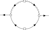
(b)

(c)

Figure 4: Contributions to the density response and density correlation that arise from the coupling to the momentum density. Fig. (a) and (b) show the retarded function and correlation function at leading order in the advective couplings. Fig. (c) shows the vertex function for the composite operator $X$ that appears in the FD relation.

In this Section we consider corrections to the density response induced by the coupling to the momentum density. These terms are of interest for two reasons: 1) As we will see, the coupling to $\pi_{k}$ generates the leading hydrodynamic tail in the density response, and 2) in a critical fluid the order parameter relaxation rate is dominated by the coupling to the momentum density (the corresponding momentum dependent relaxation rate is known as the Kawasaki function Kawasaki [1970]).

Feynman diagrams for the leading order corrections to the response and correlation functions are shown in Fig. 4. The retarded functions for the momentum density is given by

$$G_{\pi,0}^{ij}(\omega,k)=\langle\tilde{\pi}^{i}\pi^{j}\rangle_{\omega,k}=\frac{P^{ij}_{\perp}(k)}{-i\omega+\gamma_{0}k^{2}}\,,\hskip 14.22636ptP^{ij}_{\perp}(k)=\delta^{ij}-\hat{k}^{i}\hat{k}^{j}\,,$$ (40)

where $P^{ij}_{\perp}(k)$ is a transverse projection operator and $\hat{k}=\vec{k}/|\vec{k}|$ is a unit momentum vector. The correlation function is

$$C_{\pi,0}^{ij}(\omega,k)=\langle\pi^{i}\pi^{j}\rangle_{\omega,k}=\frac{2\gamma_{0}wk^{2}P_{\perp}^{ij}(k)}{\omega^{2}+(\gamma_{0}k^{2})^{2}}$$ (41)

and the interaction vertices are summarized in Fig. 3. Fig. 4(a) corresponds to a self energy term. We get

$$\Sigma(\omega,k)=\frac{1}{6\pi}\frac{k^{2}}{w(\gamma_{0}+D_{0})}\sqrt{\frac{-i\omega}{\gamma_{0}+D_{0}}}\,,$$ (42)

where, for simplicity, we have expanded the result to leading order in $k^{2}$ for $\omega\neq 0$. We can reinstate the temperature by replacing $w\to w/T$. Note that this result is more important, in the sense of the gradient expansion, than the contribution from non-linear interactions and multiplicative noise, see equ. (20). Equ. (42) determines the leading hydrodynamic tail in the density response, and it has been computed many times in the literature, see De Schepper et al. [1974], Kovtun and Yaffe [2003], Kovtun [2012], Martinez and Schäfer [2019]. The fact that equ. (42) is lower order in $k^{2}$ compared to equ. (20) can be traced to the fact that mode coupling vertices are $O(k)$, whereas the non-linear interaction and noise vertices are $O(k^{2})$.

The one-loop correction to the correlation function is shown in Fig. 4(b). This diagram can be viewed as a contribution to $\delta D$ in equ. (21). We find

$$\delta D(\omega,k)=\frac{1}{3\pi}\frac{k^{2}}{w(\gamma_{0}+D_{0})}\;{\mathrm{Re}}\,\,\sqrt{\frac{-i\omega}{\gamma_{0}+D_{0}}}\,.$$ (43)

Equ. (42) and (43) do not satisfy naive FD relation. Instead, we have to include the contribution of the vertex function $\Gamma_{X}$, given by

$$\Gamma_{X}(\omega,k)=\frac{1}{6\pi}\frac{k^{2}}{w(\gamma_{0}+D_{0})}\sqrt{\frac{-i\omega}{\gamma_{0}+D_{0}}}\,.$$ (44)

We can now verify that the extended FD relation (38) is satisfied. We also note that Figs. 2 and 4 comprise the full set of one-loop corrections to the density response in the presence of advection and multiplicative noise. We note, in particular that multiplicative noise does not modify the leading order result in equ. (42). This means that it does not modify the Kawasaki function, which is the self energy $\Sigma(\omega,k)$ in the limit $\omega\to 0$ and $r\to 0$. The Kawasaki function governs the dynamical critical exponent $z\simeq 3$ of model H Hohenberg and Halperin [1977], Onuki [2002].

6 Renormalization of the shear viscosity

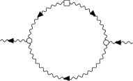
(a)

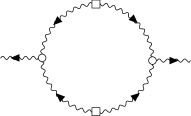
(b)

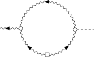
(c)

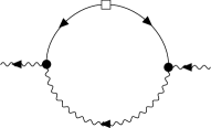
(d)

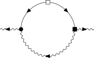
(e)

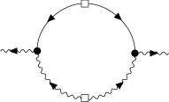
(f)

(g)

Figure 5: One-loop contributions to the response and correlation function in model H. Diagrams (a) and (b) contain the mode coupling interaction, diagram (c) is the vertex function that appears in the FD relation, and diagrams (d)-(g) are induced by multiplicative noise.

In this Section we study the response function of the transverse momentum density. At tree level, this response is controlled by the momentum diffusion constant $\gamma_{0}=\eta/w$. The leading correction to the response arises from the diagram in Fig. 5(a). This diagram corresponds to a self energy term. We define the transverse self energy $\Sigma_{T}$ by $\Sigma^{ij}=\Sigma_{T}P_{\perp}^{ij}(k)+\Sigma_{L}\hat{k}^{i}\hat{k}^{j}$ and find

$$\Sigma_{T}(\omega,k)=\frac{7}{120\pi}\frac{k^{2}}{w\gamma_{0}}\sqrt{\frac{-i\omega}{2\gamma_{0}}}\,,$$ (45)

where we have expanded the result to leading order in $k^{2}$ for $\omega\neq 0$, and we can reinstate the temperature by replacing $w\to w/T$. As before, we do not explicitly write a frequency independent term that is linearly divergent in the cutoff $\Lambda$. This contribution can be viewed as a term that combines with the bare momentum diffusion constant to provide the physical diffusivity. Equ. (45) determines the leading hydrodynamic tail in the stress tensor correlation function in a theory with only shear modes. The numerical coefficient in equ. (45) agrees with the result in Kovtun et al. [2011], Chafin and Schäfer [2013], Akamatsu et al. [2017], Martinez and Schäfer [2019]. Fig. 5(b) shows the corresponding contribution to the correlation function. In analogy with equ. (21) we define a correction $\delta\gamma$ to the numerator of the correlation function. We obtain

$$\delta\gamma_{T}(\omega,k)=\frac{7}{60\pi}\frac{k^{2}}{w\gamma_{0}}\,{\mathrm{Re}}\,\,\sqrt{\frac{-i\omega}{2\gamma_{0}}}\,.$$ (46)

In order to satisfy the FD relation we have to include a new vertex function $\Gamma_{Y}$, where the composite operator $Y$ is given by $Y_{k}=\tilde{\pi}_{i}\nabla_{k}\pi_{i}-\tilde{\pi}_{i}\nabla_{i}\pi_{k}$. The structure of $Y_{k}$ follows from the symmetry of the Poisson bracket $\{\pi_{i},\pi_{k}\}$. The vertex function $\Gamma_{Y}$ is defined by

$$\Gamma_{Y,T}(\omega,k)=\left(-i\omega+\gamma_{0}k^{2}\right)P_{jk}^{\perp}(k)\left\langle\pi_{j}Y_{k}\right\rangle_{\omega,k}$$ (47)

Computing the diagram in Fig. 5(c) we obtain

$$\Gamma_{Y,T}(\omega,k)=\frac{7}{120\pi}\frac{k^{2}}{w\gamma_{0}}\sqrt{\frac{-i\omega}{2\gamma_{0}}}\,.$$ (48)

This result satisfies the FD relation

$$2\,{\mathrm{Im}}\,\left\{G_{T}(\omega,k)\left[\gamma_{0}wk^{2}+\Gamma_{Y,T}(\omega,k)\right]\right\}=\omega C_{T}(\omega,k)\,,$$ (49)

where $G_{T}$ and $C_{T}$ denote the transverse retarded function and correlation function, respectively. We note that there is a higher order correction to equ. (45,46) that arises from the $O(\nabla^{2})$ mode coupling to $\psi$ in equ. (34). We do not study this term here.

Fig. 5(d) shows the leading correction to the transverse self energy due to multiplicative noise. Fig. 5(e,f,g) are the corresponding corrections to the correlation and vertex function. The self energy is

$$\Sigma_{T}(\omega,k)=\frac{(\gamma_{0}\lambda_{\eta})^{2}}{15\pi w}\;k^{2}\;\left(\frac{-i\omega}{\gamma_{0}+D_{0}}\right)^{3/2}\,.$$ (50)

Here, we have expanded $\Sigma_{T}(\omega,k)$ to leading order in $k^{2}$ for $\omega\neq 0$. We have also dropped cutoff dependent terms that renormalize the transport coefficients. We observe that multiplicative noise modifies the low frequency behavior of the shear viscosity, but that this correction is subleading compared to equ. (45). It is known that in model H the critical enhancement of the shear viscosity is very weak Onuki [2002]. Our results indicate that this result is not modified by multiplicative noise.

7 Conclusions and outlook

In this work we studied the role of multiplicative noise in the theory of a conserved density coupled to the transverse momentum density of a fluid. This theory governs the critical behavior of both ordinary fluids Hohenberg and Halperin [1977] and the quark gluon plasma Son and Stephanov [2004] in the vicinity of a possible critical end point. In this context we can think of $\psi$ as the entropy per particle of the fluid. Multiplicative noise arises from the dependence of the thermal conductivity and shear viscosity on $\psi$.

Multiplicative noise is consistent with suitably generalized fluctuation-dissipation relations. It also fits into the standard long time, large wavelength, expansion of hydrodynamic correlation functions. We find that multiplicative noise contributes to the long-time tails of the density and momentum density correlation functions. In model B, without the coupling to the momentum density, this contribution is leading order. In model H the multiplicative noise contribution to the tails is subleading compared to the contributions induced by mode couplings. At leading order in $k$ multiplicative noise does not modify the Kawasaki function, which governs the order parameter relaxation rate in model H Hohenberg and Halperin [1977], or the self energy of transverse momentum modes, which determines the renormalization of the shear viscosity.

In the present work we have used diagrammatic methods to study correlation functions in a fluid at rest, or in the local restframe of a slowly evolving background flow. These results are applicable to both relativistic and non-relativistic systems. We have not addressed the issue of writing the effective action in a manifestly covariant way Kovtun et al. [2014], or investigated correlation functions in an evolving background Akamatsu et al. [2017], An et al. [2019]. We have also not studied the coupling to sound modes, and the renormalization of the bulk viscosity in a non-conformal fluid Kovtun and Yaffe [2003], Martinez and Schäfer [2017], Akamatsu et al. [2018], Martinez et al. [2019]. Finally, it would be interesting to study multiplicative noise in numerical simulations of stochastic diffusion in an expanding fluid Nahrgang et al. [2019].

Appendix A Fluctuation-Dissipation relation

In this appendix we derive the fluctuation-dissipation (FD) relation in model B in the presence of multiplicative noise, following the method described in Janssen [1979], Täuber [2014]. For this purpose we compute the response function Equ. (13) in two different ways. The first is based on coupling an external source to the MSRJD functional. The source term in the effective Lagrangian equ. (6) is ${\cal L}_{h}=\tilde{\psi}(x,t)L(\psi)h(x,t)$, where $L(\psi)$ is defined in equ. (7). We can then compute the response function

$$G_{R}(x_{1},t_{1};x_{2},t_{2})=\left\langle\psi(x_{1},t_{1})\left[L(\psi)\tilde{\psi}\right](x_{2},t_{2})\right\rangle\,.$$ (51)

The second method is based on the noise average in equ. (4). Formally, we can express the noise in terms of the diffusion equation,

$$\theta(x,t)=\partial_{t}\psi(x,t)+L(\psi)\frac{\delta{\cal F}[\psi]}{\delta\psi}\,.$$ (52)

This implies that we perform the average over solutions of the diffusion equation with respect to the noise distribution in equ. (4) by changing variables from $\theta(x,t)$ to $\psi(x,t)$. The corresponding partition function is

$$Z_{OM}=\int{\cal D}\psi\,\exp\left(-S_{OM}(\psi)\right)\,,$$ (53)

where $S_{OM}$, the Onsager-Machlup functional, is given by

$$S_{OM}=-\frac{1}{4}\int dt\,dx\,\left(\partial_{t}\psi+L(\psi)\frac{\delta{\cal F}[\psi]}{\delta\psi}\right)\left[L(\psi)\right]^{-1}\left(\partial_{t}\psi+L(\psi)\frac{\delta{\cal F}[\psi]}{\delta\psi}\right)\,.$$ (54)

Computing the response fucntion using equ. (53) we obtain

$$G_{R}(x_{1},t_{1};x_{2},t_{2})=\frac{1}{2}\left\langle\psi(x_{1},t_{1})\left[\partial_{t}\psi+L(\psi)\frac{\delta{\cal F}[\psi]}{\delta\psi}\right](x_{2},t_{2})\right\rangle\,.$$ (55)

In the following, we will denote $U[\psi]=L(\psi)(\delta F[\psi])/(\delta\psi)$. The response function is retarded and satisfies

$$G_{R}(x_{1},t_{1};x_{2},t_{2})=\frac{1}{2}\left\langle\psi(x_{1},t_{1})\left[\partial_{t}\psi+U[\psi]\right](x_{2},t_{2})\right\rangle=0\,,\;\;t_{1}<t_{2}\,.$$ (56)

so that

$$\left\langle\psi(x_{1},t_{1})\partial_{t}\psi(x_{2},t)\right\rangle-\left\langle\psi(x_{1},t_{1})U[\psi](x_{2},t)\right\rangle=0\,,\;\;t_{1}<t\,.$$ (57)

We can now analzye the behavior of equ. (57) under the T-reversal symmetry defined in equ. (8,9). We find that the first term is even, whereas the second term is odd, so that for $t_{1}>t$ the two terms in equ. (56) contribute equally. Comparing equ. (51) and equ. (56) then implies the fluctuation-dissipation relation

$$\left\langle\psi(x_{1},t_{1})\left[L(\psi)\tilde{\psi}\right](x_{2},t_{2})\right\rangle=\Theta(t_{2}-t_{1})\left\langle\psi(x_{1},t_{1})\dot{\psi}(x_{2},t_{2})\right\rangle$$ (58)

given in equ. (14). This relation can be generalized to more complicated response functions, and to model H.

References

- Romatschke and Romatschke [2019] Paul Romatschke and Ulrike Romatschke. Relativistic Fluid Dynamics In and Out of Equilibrium. Cambridge Monographs on Mathematical Physics. Cambridge University Press, 5 2019.
- Jeon and Heinz [2015] Sangyong Jeon and Ulrich Heinz. Introduction to Hydrodynamics. Int. J. Mod. Phys. E, 24(10):1530010, 2015.
- Teaney [2010] Derek A. Teaney. Viscous Hydrodynamics and the Quark Gluon Plasma, pages 207–266. World Scientific (R. Hwa and X. N. Wang, editors), 2010.
- De Schepper et al. [1974] I. M. De Schepper, H. Van Beyeren, and M. H. Ernst. The nonexistence of the linear diffusion equation beyond Fick’s law. Physica, 75:1, 1974.
- Pomeau and Resibois [1975] Yves Pomeau and Pierre Resibois. Time dependent correlation functions and mode-mode coupling theories. Physics Reports, 19(2):63–139, 1975.
- Kovtun and Yaffe [2003] Pavel Kovtun and Laurence G. Yaffe. Hydrodynamic fluctuations, long time tails, and supersymmetry. Phys. Rev., D68:025007, 2003.
- Peralta-Ramos and Calzetta [2012] J. Peralta-Ramos and E. Calzetta. Shear viscosity from thermal fluctuations in relativistic conformal fluid dynamics. JHEP, 02:085, 2012.
- Kovtun et al. [2011] Pavel Kovtun, Guy D. Moore, and Paul Romatschke. The stickiness of sound: An absolute lower limit on viscosity and the breakdown of second order relativistic hydrodynamics. Phys. Rev., D84:025006, 2011.
- Kapusta et al. [2012] J. I. Kapusta, B. Muller, and M. Stephanov. Relativistic Theory of Hydrodynamic Fluctuations with Applications to Heavy Ion Collisions. Phys. Rev., C85:054906, 2012.
- Kovtun [2012] Pavel Kovtun. Lectures on hydrodynamic fluctuations in relativistic theories. J. Phys., A45:473001, 2012.
- Chafin and Schäfer [2013] Clifford Chafin and Thomas Schäfer. Hydrodynamic fluctuations and the minimum shear viscosity of the dilute Fermi gas at unitarity. Phys. Rev., A87(2):023629, 2013.
- Akamatsu et al. [2017] Yukinao Akamatsu, Aleksas Mazeliauskas, and Derek Teaney. A kinetic regime of hydrodynamic fluctuations and long time tails for a Bjorken expansion. Phys. Rev., C95(1):014909, 2017.
- Martinez and Schäfer [2019] Mauricio Martinez and Thomas Schäfer. Stochastic hydrodynamics and long time tails of an expanding conformal charged fluid. Phys. Rev. C, 99(5):054902, 2019.
- Chen-Lin et al. [2019] Xinyi Chen-Lin, Luca V. Delacrétaz, and Sean A. Hartnoll. Theory of diffusive fluctuations. Phys. Rev. Lett., 122(9):091602, 2019.
- Akamatsu et al. [2019] Yukinao Akamatsu, Derek Teaney, Fanglida Yan, and Yi Yin. Transits of the QCD critical point. Phys. Rev. C, 100(4):044901, 2019.
- An et al. [2019] Xin An, Gokce Basar, Mikhail Stephanov, and Ho-Ung Yee. Relativistic Hydrodynamic Fluctuations. Phys. Rev. C, 100(2):024910, 2019.
- Wang and Heinz [2002] Enke Wang and Ulrich W. Heinz. A Generalized fluctuation dissipation theorem for nonlinear response functions. Phys. Rev. D, 66:025008, 2002.
- Habib [1993] Salman Habib. Multiplicative noise: Applications in cosmology and field theory. Annals N. Y. Acad. Sci., 706:111, 1993.
- Arnold [2000a] Peter Brockway Arnold. Symmetric path integrals for stochastic equations with multiplicative noise. Phys. Rev. E, 61:6099–6102, 2000a.
- Arnold [2000b] Peter Brockway Arnold. Langevin equations with multiplicative noise: Resolution of time discretization ambiguities for equilibrium systems. Phys. Rev. E, 61:6091–6098, 2000b.
- Aron et al. [2010] Camille Aron, Giulio Biroli, and Leticia F. Cugliandolo. Symmetries of generating functionals of Langevin processes with colored multiplicative noise. J. Stat. Mech., 1011:P11018, 2010.
- Arenas and Barci [2012] Zochil Gonzalez Arenas and Daniel G. Barci. Hidden symmetries and equilibrium properties of multiplicative white-noise stochastic processes. J. Stat. Mech., 1212(12):P12005, 2012.
- Biro and Jakovac [2005] Tamas S. Biro and Antal Jakovac. Power-law tails from multiplicative noise. Phys. Rev. Lett., 94:132302, 2005.
- Hohenberg and Halperin [1977] P.C. Hohenberg and B.I. Halperin. Theory of Dynamic Critical Phenomena. Rev. Mod. Phys., 49:435–479, 1977.
- Martin et al. [1973] P.C. Martin, E.D. Siggia, and H.A. Rose. Statistical Dynamics of Classical Systems. Phys. Rev. A, 8:423–437, 1973.
- Janssen [1976] Hans-Karl Janssen. On a lagrangean for classical field dynamics and renormalization group calculations of dynamical critical properties. Zeitschrift für Physik B, 23:377–380, 1976.
- De Dominicis and Peliti [1978] C. De Dominicis and L. Peliti. Field Theory Renormalization and Critical Dynamics Above t(c): Helium, Antiferromagnets and Liquid Gas Systems. Phys. Rev. B, 18:353–376, 1978.
- Täuber [2014] Uwe C Täuber. Critical dynamics: a field theory approach to equilibrium and non-equilibrium scaling behavior. Cambridge University Press, 2014.
- Bausch et al. [1976] R. Bausch, H. K. Janssen, and H. Wagner. Renormalized field theory of critical dynamics. Z. Physik B, 24:113–127, 1976.
- Janssen [1979] H. K. Janssen. Field-theoretic method applied to critical dynamics. In Charles P. Enz, editor, Dynamical Critical Phenomena and Related Topics, volume 104, page 25. Springer Berlin Heidelberg, 1979.
- Crossley et al. [2017] Michael Crossley, Paolo Glorioso, and Hong Liu. Effective field theory of dissipative fluids. JHEP, 09:095, 2017.
- Glorioso et al. [2017] Paolo Glorioso, Michael Crossley, and Hong Liu. Effective field theory of dissipative fluids (II): classical limit, dynamical KMS symmetry and entropy current. JHEP, 09:096, 2017.
- Dzyaloshinskii and Volovick [1980] I. E. Dzyaloshinskii and G. E. Volovick. Poisson brackets in condensed matter physics. Annals of Physics, 125(1):67–97, 1980.
- Kawasaki [1970] K. Kawasaki. Kinetic equations and time correlation functions of critical fluctuations. Ann. Phys., 61:1, 1970.
- Onuki [2002] Akira Onuki. Phase transition dynamics. Cambridge University Press, 2002.
- Son and Stephanov [2004] D.T. Son and M.A. Stephanov. Dynamic universality class of the QCD critical point. Phys. Rev. D, 70:056001, 2004.
- Kovtun et al. [2014] Pavel Kovtun, Guy D. Moore, and Paul Romatschke. Towards an effective action for relativistic dissipative hydrodynamics. J. High Energ. Phys., 2014(7):123, 2014.
- Martinez and Schäfer [2017] Mauricio Martinez and Thomas Schäfer. Hydrodynamic tails and a fluctuation bound on the bulk viscosity. Phys. Rev. A, 96(6):063607, 2017.
- Akamatsu et al. [2018] Yukinao Akamatsu, Aleksas Mazeliauskas, and Derek Teaney. Bulk viscosity from hydrodynamic fluctuations with relativistic hydrokinetic theory. Phys. Rev. C, 97(2):024902, 2018.
- Martinez et al. [2019] M. Martinez, T. Schäfer, and V. Skokov. Critical behavior of the bulk viscosity in QCD. Phys. Rev. D, 100(7):074017, 2019.
- Nahrgang et al. [2019] Marlene Nahrgang, Marcus Bluhm, Thomas Schäfer, and Steffen A. Bass. Diffusive dynamics of critical fluctuations near the QCD critical point. Phys. Rev. D, 99(11):116015, 2019.