Enhancing the sensitivity of transient gravitational wave searches with Gaussian Mixture Models

Abstract

Identifying the presence of a gravitational wave transient buried in non-stationary, non-Gaussian noise which can often contain spurious noise transients (glitches) is a very challenging task. For a given data set, transient gravitational wave searches produce a corresponding list of triggers that indicate the possible presence of a gravitational wave signal. These triggers are often the result of glitches mimicking gravitational wave signal characteristics. To distinguish glitches from genuine gravitational wave signals, search algorithms estimate a range of trigger attributes, with thresholds applied to these trigger properties to separate signal from noise. Here, we present the use of Gaussian mixture models, a supervised machine learning approach, as a means of modelling the multi-dimensional trigger attribute space. We demonstrate this approach by applying it to triggers from the coherent Waveburst search for generic bursts in LIGO O1 data. By building Gaussian mixture models for the signal and background noise attribute spaces, we show that we can significantly improve the sensitivity of the coherent Waveburst search and strongly suppress the impact of glitches and background noise, without the use of multiple search bins as employed by the original O1 search. We show that the detection probability is enhanced by a factor of 10, leading enhanced statistical significance for gravitational wave signals such as GW150914.

I Introduction

The era of gravitational-wave (GW) astronomy began with the first direct detection of the GW signal observed on September 14, 2015 Abbott et al. (2017a) by the Advanced LIGO Aasi et al. (2015) and Virgo Acernese et al. (2015) detectors. So far, in the proceeding observing runs, the LIGO Scientific and Virgo Collaboration have fourteen confirmed GW detections Abbott et al. (2016a, b, 2017b, 2017c, 2017a, c, 2018, 2017d, 2020), with data from several further candidate compact binary merger candidates still being analyzed. In the next few years, the Advanced LIGO and Virgo detectors will improve in sensitivity, and additional GW detectors such as KAGRA Aso et al. (2013), and LIGO-India Iyer et al. (2011) will join the network. The sensitivity improvement of the GW detector network will lead to more detections of GWs from different types of source Davis et al. (2020).

With improved detector perfromance, GW detectors are becoming more sensitive to other disturbances culminating in the observation of a large number of non-Gaussian noise transients known as glitches Abbott et al. (2016d). They originate due to complex instrumental and environmental effects within GW detectors. Often, they produce high signal-to-noise ratio (SNR) triggers in GW searches, increasing false alarm rates and reducing search sensitivity. Data quality investigations Nuttall et al. (2015) that focus on the correlation between instrument or environmental effects with GW data as well as veto techniques have helped to eliminate some known glitch classes. However, a large number of unknown noisy transients persist. Different searches explore different types of glitch rejection methods Allen (2005); Nitz (2018); Dal Canton et al. (2014); Gayathri et al. (2019) to improve search sensitivity. Though important, these methods also increase the computational burden of existing GW detection algorithms.

The volume of literature on the application of machine learning methods in GW astrophsyics is rapdily growing. This includes techniques to improve signal detection, parameter estimation of transient signals, noise removal techniques, modeling GW signals as well as source population inference Bahaadini et al. (2018); Mukund et al. (2017); Colgan et al. (2020); Cuoco et al. (2020); Vajente et al. (2020); George and Huerta (2018); Gebhard et al. (2019); Gabbard et al. (2019); Cuoco et al. (2020).

In this work, we propose a supervised machine learning method using Gaussian mixture models (GMMs) for use in signal detection where we construct two distinct models for noise glitches and astrophysical GW signals. Rather than developing this approach using time-series data, we instead apply it after the coherent Waveburst (cWB) algorithm has identified triggers – interesting time instances which could be either potential GW signals or the noisy transients. At present, the cWB search algorithm has multiple output attributes and based on the location of the trigger attributes in this multi-dimentional space, the trigger is classified as a GW event or noisy event. We propose an alternative to the existing thresholding procedure on the multi-dimentional attribute space by folding in the GMM naturally in the detection problem under the likelihood ratio approach.

The paper is organized as follows : In Sec. II, we discuss the Gaussian mixture modelling of the multi-modal data set. In Sec. III we discuss the use of the GMM in the construction of a log-likelihood based detection statistic. In Sec. IV we assess the detection performance of the proposed GMM based detection method with respect to the generic burst algorithm in an all-sky short-duration GW burst set-up. We apply the algorithm for the coincident events from the first observing run of advanced LIGO detectors. Finally, in Sec. V, we discuss our conclusions.

II Gaussian mixture model

Gaussian mixture models (GMMs) are probabilistic models which use uni-modal Gaussian distributions to represent a multi-modal data set. Under the GMM approach, a given data set is modelled as a weighted sum of a collection of Gaussians.

Let the data vector ${\bf x}$ be characterized by $d$ number of attributes. We refer to these data as a $d$-dimensional data vector. The corresponding GMM of the data consists of a superposition of $K$ Gaussian distributions and is given by

$$p({\bf x})=\sum_{j=1}^{K}w_{j}\mathcal{N}({\bf x}|\boldsymbol{\mu_{j}},\Sigma_{j}),$$ (1)

where, $\mathcal{N}({\bf x}|\boldsymbol{\mu_{j}},\Sigma_{j})$ is a multinomial Gaussian distribution with $d$-dimensional mean vector $\boldsymbol{\mu_{j}}$ and $d\times d$ co-variance matrix $\Sigma_{j}$ and is written as

$$\mathcal{N}({\bf x}|\boldsymbol{\mu_{j}},\Sigma_{j})=\frac{\exp\left[-\frac{1}{2}({\bf x}-\boldsymbol{\mu_{j}})^{T}\Sigma_{j}^{-1}({\bf x}-\boldsymbol{\mu_{j}})\right]}{(2\pi)^{d/2}|\Sigma_{j}|^{1/2}}.$$ (2)

The parameter $w_{j}$ is the weight corresponding to each Gaussian component normalised such that $\sum_{j}w_{j}=1$.

When the data is believed to contain two distinct populations but where each population has complex but distinct structure within the attribute space, GMMs can be used to model each population separately. These models can be then incorporated into a likelihood-ratio test statistic which can be used to identify events from either population. This is classed as an supervised machine learning algorithm.

III Detection method using GMM

In the GW signal detection problem, signal events and noisy background events are considered as two distinct populations. In this section, we describe the use of GMMs to model these populations and the development of a detection statistic based on this.

III.1 Log-Likelihood statistic

Let us consider the data set with $n$ $d$-dimensional data points as ${\bf X}=\{{\bf x}_{1},{\bf x}_{2},\dots\bf x_{n}\}$. We assume that each of the ${\bf x}_{i}$’s are independent and we represent ${\bf X}$ as an $n\times d$ matrix. The likelihood function can then be written as,

$$p({\bf X}|\bm{\theta})=\prod_{i=1}^{n}p({\bf x}_{i}|\bm{\Theta}),\quad$$ (3)

where parameters $\Theta:=w_{j},\boldsymbol{\mu_{j}},\Sigma_{j},\{j=1,...,K\}$. Then the corresponding total log-likelihood is the sum of $n$ individual log-likelihoods as given below,

$$\ln\mathcal{L}=\sum_{i=1}^{n}\ln(p({\bf x}_{i}|\bm{\Theta}))=\sum_{i=1}^{n}\ln\left\{\sum_{j=1}^{K}w_{j}\mathcal{N}\left({\bf x}_{i}|\boldsymbol{\mu_{j}},\Sigma_{j}\right)\right\}\,.$$ (4)

III.2 Maximum likelihood approach

To estimate the model parameters $\Theta$ we can maximize $\ln\mathcal{L}$ with respect to each of these parameters. For example,

$$\frac{\partial\ln\mathcal{L}}{\partial\boldsymbol{\mu_{j}}}=0\leavevmode\nobreak\ \leavevmode\nobreak\ \leavevmode\nobreak\ \Rightarrow\leavevmode\nobreak\ \leavevmode\nobreak\ \leavevmode\nobreak\ \boldsymbol{\hat{\mu}_{k}} =\frac{\sum_{i=1}^{n}r_{ik}{\bf x}_{i}}{N_{k}},$$ (5)

where

$$r_{ik} =\frac{w_{k}\mathcal{N}\left({\bf x}_{i}|\boldsymbol{\mu_{k}},\Sigma_{k}\right)}{\sum_{j=1}w_{j}\mathcal{N}\left({\bf x}_{i}|\boldsymbol{\mu_{j}},\Sigma_{j}\right)}\hskip 5.69046pt\text{and}\hskip 5.69046ptN_{k}=\sum_{i=1}^{n}r_{ik}.$$ (6)

Thus the maximum likelihood estimate of the mean $\boldsymbol{\mu_{k}}$ of the $k^{\text{th}}$ Gaussian is the weighted mean of all the data points. All the coefficients are implicit functions of ${\boldsymbol{\mu_{k}}}$ via the normal distributions.

Similarly, maximizing $\ln\mathcal{L}$ with respect to the co-variance matrix $\Sigma_{k}$, of the $k^{th}$ Gaussian, we obtain

$${\hat{\Sigma}}_{k}=\frac{1}{N_{k}}\sum_{i=1}^{n}r_{ik}\left({\bf x}_{i}-{\boldsymbol{\mu_{k}}}\right)\left({\bf x}_{i}-\boldsymbol{\mu_{k}}\right)^{T}.$$ (7)

Maximization of Eq.4 over $w_{j}$ under the constrain that sum of the weights add up to unity can be obtained through the application of Lagrange multipliers. The details can be found in Appendix A. This gives the maximum likelihood estimate for weights as

$$\hat{w}_{k} =\frac{\sum_{i=1}^{n}r_{ik}}{n}=\frac{N_{k}}{n}.$$ (8)

It is clear from above calculation that it is difficult to analytically estimate the parameters of the mixture model as all the estimates given in Eq. 8 are implicit functions of themselves.

The Expectation maximization (EM) technique Dempster et al. (1977) is an iterative algorithm and provides us with a numerical solution to our maximum likelihood problem. The EM algorithm has two steps, namely the estimation step and the maximization step. The first step involves using trial values for the parameters, then, using these values an iterative step using Eqs. (5, 7, 8) gives estimates of the new values of the parameters. Thus, iteratively using Eqs. (5, 7, 8), the EM algorithm convergences on the maximum-likelihood parameters $\hat{\Theta}$.

A drawback of the EM algorithm is that it cannot predict the optimal number of Gaussians required to describe the underlying structure of the data. Large numbers of Gaussians can lead to overfitting of the data. The Bayesian information criterion (BIC) includes a penalty term which compensates this effect and is used in the model selection.

The BIC as defined in terms of the maximum value of the likelihood function $\hat{\mathcal{L}}$ and is given by

$${\rm BIC} =K\ln(n)-2\ln(\hat{\mathcal{L}}).$$ (9)

where the first term in Eq. 9 is the desired penalty term. The lowest BIC score provides the optimum number of Gaussians $\hat{K}$ for a given data set.

III.3 GMM based detection statistic

Once all the model parameters $\Theta$ are optimally chosen and the optimum number of Gaussians are fixed following the minimum BIC criterion detailed in the previous subsection, we write the maximum log-likelihood statistic as $W=\ln(\hat{\mathcal{L}})|_{\hat{K}}$.

Since our data consists of two distinct classes, signals (s) and noisy background glitches (g), we can calculate a detection statistic, $T$, for each trigger such that

$$T=W_{\text{s}}-W_{\text{g}}\,.$$ (10)

GMM based models each for the signal and noise are required to determine $W_{\text{s}}$ and $W_{\text{g}}$ respectively. In line with tuning and training procedures for cWB and other transient searches, the characterisation and optimisation of the GMM performance is done a prior on training data, prior to the search for gravitational wave candidates. To calculate $W_{\text{g}}$, we first construct a GMM model using the noise background data. The noise background data are divided into a training data set, which is used to construct the GMM model, and a validation data set. Similarly, for $W_{\text{s}}$, we construct a GMM model using simulated signals which are also divided into training and validation sets. We compute the test statistic $T$ for the validation noise set and validation simulation trigger set and we assess the performance of the GMM models by comparing the detection probability against the false alarm probability. Note that the validation data set allows us to check that the GMM model is overfitting the signal parameter space since it is vital for a generic transient search to be sensitive to a wide range of signal morphologies.

IV Short duration GW burst search with GMM

A large variety of GW transients fall into the category of short duration bursts e.g., GWs from supernovae, merger of binary black holes etc. In fact, the first observed GW signal from a binary black hole merger (GW150914) was indeed first detected by a generic burst search algorithm coherent Waveburst (cWB) Abbott et al. (2016a). Typically, the cWB burst search method finds interesting and potential GW events at an initial analysis stage which we refer as triggers. To obtain an estimate of the noise background and assign each trigger a statistical significance, the cWB analysis is performed on data that is time-shifted so that it is unphysical for a gravitational wave signal be detected in coincidence between detectors. The noise background rate is determined by the number of triggers observed in the time-shifted data. Triggers observed in data in the absence of an unphysical time shift are considered event candidates. These event candidates may be GW signals though further analysis is often required before any declaration of signal detection can be made.

To reduce the impact of noise background triggers, thresholds for various trigger attributes such as its estimated signal strength or duration are applied. To optimise the chance of detecting a GW signal, these thresholds are tuned a priori, using triggers from the time-shifted noise background and simulated signals. After applying appropriate thresholds on the trigger attributes pertaining to the search, if a given trigger emerges with high significance then it is considered a GW event. Such a thresholding procedure, though ad-hoc, is the crucial ingredient of the signal detection algorithm which helps in reducing the unwanted noisy features and select the most significant events (those with very low associated false alarm rate (FAR)) in the data set.

Here, we introduce GMMs to address this multi-dimensional attribute thresholding problem where a GMM is constructed for the signal set (and noise set) defining the characteristic features in the multi-dimentional attribute space for signal (or noise). Casting this in the log-likelihood based detection problem as outlined in Sec. III gives a natural map from this multi-dimentional approach to the scalar log-likelihood ratio. Thus, by applying a single threshold based on the test statistic across the entire multi-dimensional attribute space, we can address the ad-hoc individual attribute thresholding problem in a more systematic way. We henceforth refer to this signal detection approach as cWB plus GMM.

IV.1 Coherent Waveburst algorithm

For our data sets we consider burst-search triggers from the coherent waveburst (cWB) algorithm – a generic multi-detector, all sky burst algorithm used in GW searches that is sensitive to short duration signals Klimenko et al. (2008, 2005, 2016); Necula et al. (2012). This algorithm projects the multi-detector data into the wavelet (time-frequency map) domain using the Wilson-Daubechiers-Meyer transformation and identifies a collection of coherent time-frequency-scale pixels with excess power and clusters them based on the time-frequency information. Each burst trigger is represented by a coherent cluster and associated with a set of attributes. The attribute set contains those which characterise the signal as well as veto attributes used to help distinguish between signal and noise triggers. The complete set include estimated strain of the trigger $h_{s}$, the central frequency $f_{0}$, the duration of the trigger $\tau$, the network coherent signal-to-noise ratio $\eta_{c}$ , the network correlation coefficient $c_{c}$ which measures the correlation between the detectors, quality factor of the event $Q_{\text{veto}}$, the residual noise energy measure $\zeta^{2}$, the ratio between the reconstructed energy and the total energy $N_{\text{norm}}$, the energy dis-balance of the event between the detectors $N_{ED}$, and $L_{\text{veto}}$ which measures the localization of event in the time-frequency map.

The cWB algorithm generates a trigger list that is associated to the time-frequency clusters with high network correlation $c_{c}$ as well as cWB SNR $\eta_{c}$. Based on the type of the GW signal, the actual threshold values applied to these two parameters may vary. Following that, the cWB algorithm uses the additional thresholds on trigger attributes to veto out noisy triggers. All cWB thresholds are determined by tuning and testing on noise background and simulated signals prior before being used to generate a list of gravitational wave candidates.

IV.2 Data set

To demonstrate our method, we consider cWB triggers obtained from simulated astrophysical short-duration burst signals added to data from the first advanced detector observing run O1 Abbott et al. (2017e). Here, cWB triggers are those time-frequency clusters with $\eta_{c}>8.45$ and $c_{c}>0.5$. The 19 types of short duration signals simulated in the O1 data are Gaussian pulses (GP) characterized by duration $\tau$, sine-Gaussian wavelets (SGW) - sinusoids within a Gaussian envelope and characterized by the frequency$f_{0}$ and a quality factor $Q$, and White noise bursts (WNB) - bursts with a Gaussian envelope described by $f_{\text{low}}$, frequency bandwidth $\Delta f$, and duration $\tau$. The simulated signal parameter values used our study is listed in Table 1. The signals are uniformly distributed over the sky and with a range of selected discrete strain amplitudes from $0.5\times 10^{-21}$-$10^{-20}$. The initial phase is distributed uniformly over the range $[0,2\pi]$ and the time of arrival of the signal which depends on the sky location in relation to the detector positions is also distributed uniformly.

The final GW event list is obtained with the standard-cWB after applying thresholds on the cWB attributes and ranking them based on level of significance (ascending value of inverse false alarm rate (IFAR)). For more details on the search see Abbott et al. (2017e).

IV.3 Attribute choice

Each trigger has eleven attributes as defined in Sec. IV.2. Here, we use the exhaustive attribute set $\{c_{c0},c_{c2},\eta_{c},f_{0},h_{s},N_{\text{norm}},\zeta^{2},N_{\text{ED}},Q_{\text{veto}},L_{\text{veto}}\}$ to develop a GMM in the multi-dimentional feature attribute space and use the minimum BIC method to obtain the optimal attribute set which we use to construct the GMM for both noise as well as signal data triggers.

For a collection of $n\sim 10^{5}$ signal triggers from the data set, we consider the maximum number of Gaussian components to be $100$. We carry out an exhaustive study to build the signal model. We consider various combinations of trigger attributes starting from a set of two attributes all the way to a set of eleven attributes with a varying number of Gaussian components. We compute the lowest BIC score for a given number of attributes. For example, there are 55 combinations of pairs of attributes selected from a set of 11, 165 sets of 3 attributes selected from 11, etc. We construct the BIC for all possible combinations and choose the minimum value amongst them for a given attribute count.

This is done for each attribute count ranging from 2 to 11.

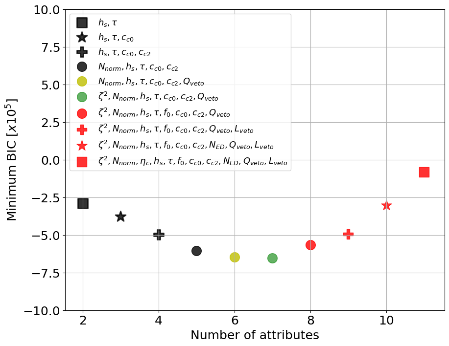
Figure 1: Plot of BIC value vs the number attributes for a given signal data set. The specific choice of attributes for each set is defined in the legend.

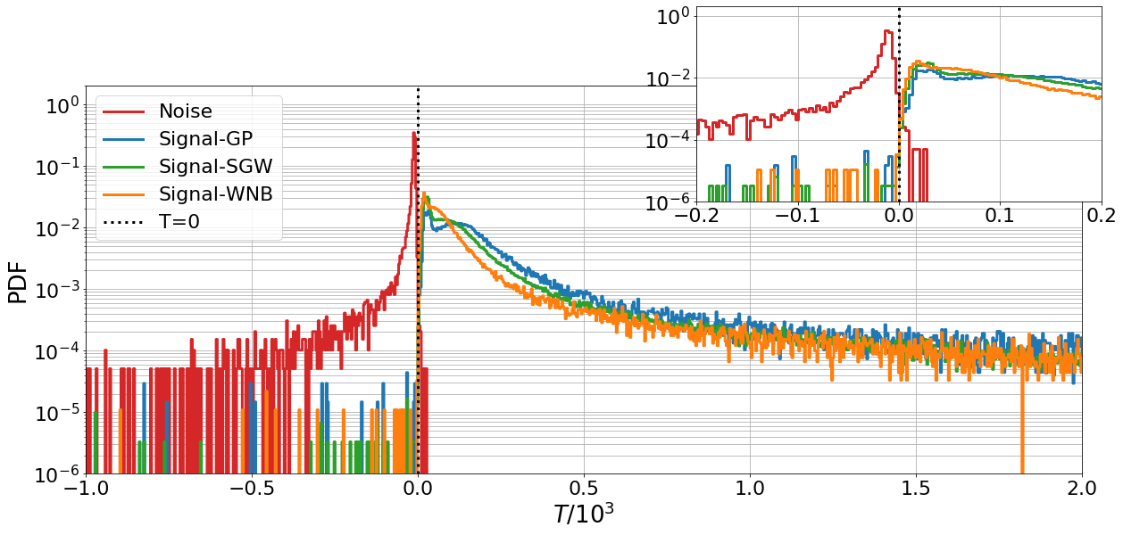
Figure 2: The $T$ value distribution for O1 noise and three different signal morphology events with GMM models. Plot contains four curves, red curve for noise, blue curve for GP, green curve for SWG and orange curve for WNB. The inset plot shows the T distribution around zero.

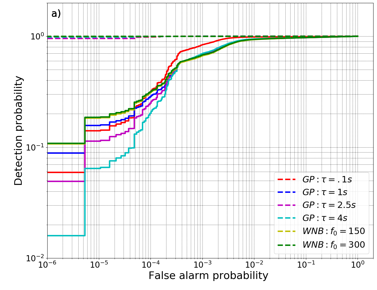
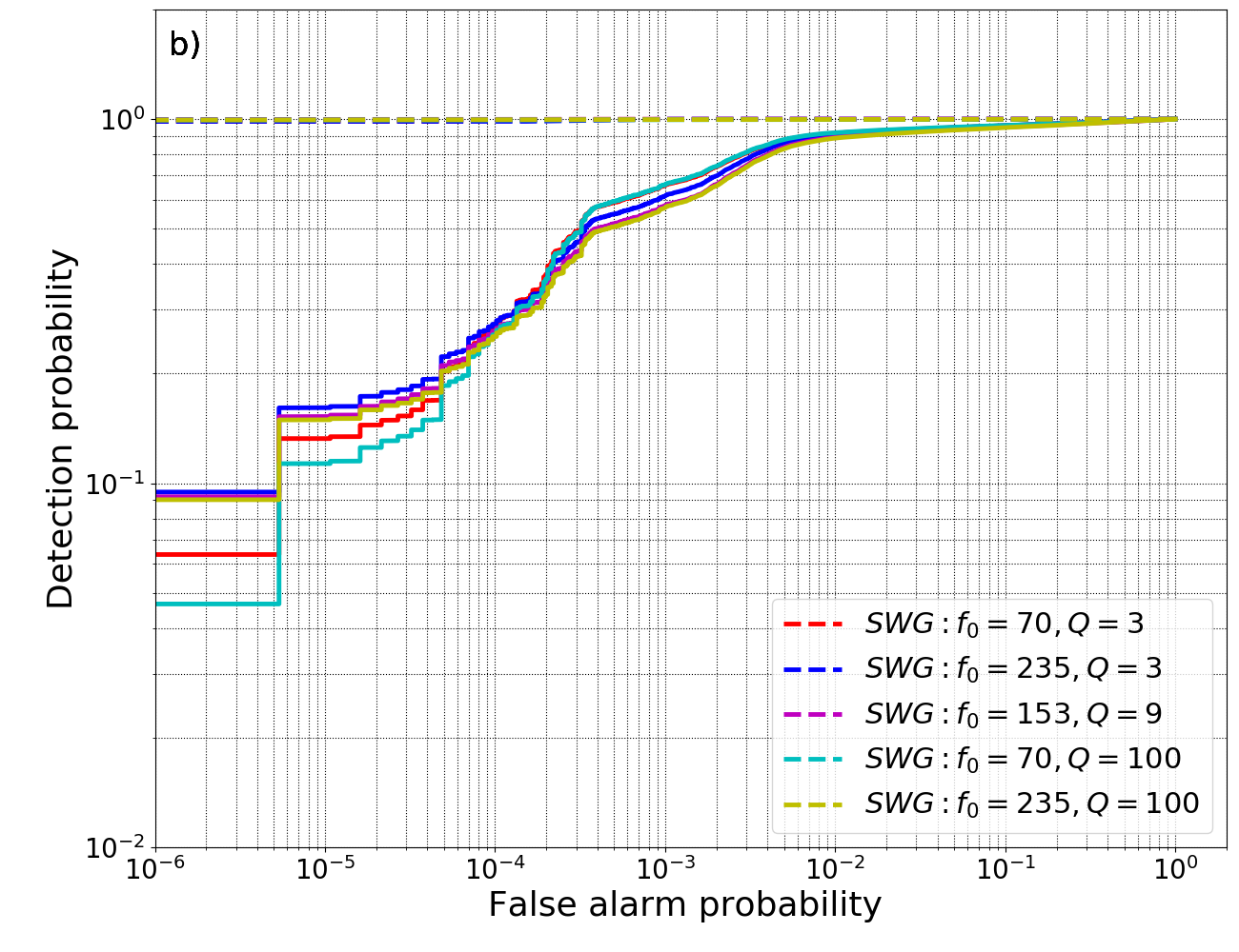
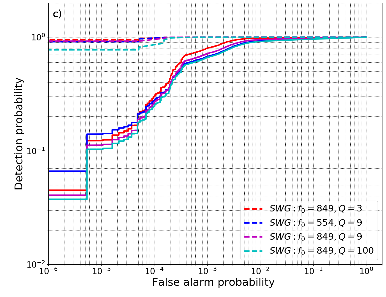
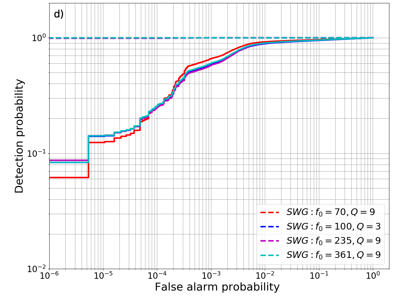
Figure 3: ROC curves: false alarm probability vs detection probability using the cWB plus GMM algorithm (dashed lines) compared to the standard-cWB pipeline (solid lines) for the simulation waveforms detailed in Table.1. We present the ROC curves in four panels by dividing the simulation sets in different types. For the cWB plus GMM analysis, the detection probability is close to 0.9 or more for almost all simulated signals, even at false alarm probabilities of $10^{-6}$.

Figure 1 shows a plot of the minimised BIC value as a function of the attribute count for the signal model. The combination of attributes shown in the legend corresponds to the minimum BIC combination for that attribute count. We note that the minima of this minimum BIC curve corresponds to the attribute set [$\zeta^{2}$, $N_{\text{norm}}$, $h_{s}$, $\tau$, $c_{c0}$, $c_{c2}$, $Q_{\text{veto}}$]– a seven attribute set which captures the signal triggers. In addition, we note that each set of $p$ optimal attributes contains within it the set of $(p-1)$ optimal attribute set. We use the attribute set corresponding to the global BIC minima to construct both the signal and noise trigger GMMs.

IV.4 Training models

As described in Sec. IV.2, the simulated signal injections span a variety of signal classes that model short bursts with a wide range of frequencies. We aim to develop a GMM for these signals that is robust against the variation in frequency and duration of the burst. To do so, we develop a minimal model which broadly captures the burst-like signals with a frequency range of $70-360$ Hz and different short durations. Thus, we choose a waveform subset from the simulation set given in table. 1 which cover the broad class of burst-like signals for model building and test the robustness of this model against the remaining waveform set. With the above rationale, our choice is a set of five burst waveforms; SGW with $f_{0}=70$Hz & $Q=3$, SGW with $f_{0}=235$Hz & $Q=9$, SGW with $f_{0}=361$Hz & $Q=9$, SGW:$f_{0}=70$Hz & $Q=100$ and GP $\tau=1$s as tabulated in the Table 1.

We choose 50% of the five selected types of burst signal triggers for training and building the GMM. The remaining signal triggers (comprising all waveform types) are used for validation, to check that the signal model is robust against varying signal morphologies. We consider 80% of noise triggers for training and building the corresponding noise GMM. The rest of the noise triggers are used for validation. This leads to the number of noise triggers for training being $\sim 10^{5}$ and signal triggers for training as $\sim 8\times 10^{4}$.

Sine-Gaussian Burst (SGW)
No.	$f_{0}$ (Hz)	$Q$	-	Training	Validation
1	70	3	-	Y	Y
2	70	9	-	N	Y
3	70	100	-	Y	Y
4	100	3	-	N	Y
5	153	9	-	N	Y
6	235	3	-	N	Y
7	235	9	-	Y	Y
8	235	100	-	N	Y
9	361	9	-	Y	Y
10	554	9	-	N	Y
11	849	3	-	N	Y
12	849	9	-	N	Y
13	849	100	-	N	Y
White-Noise Burst (WNB)
	$f_{low}$ (Hz)	$\Delta f$ (Hz)	$\tau$ (s)	Training	Validation
14	100	100	0.1	N	Y
15	300	100	0.1	N	Y
Gaussian Pulse (GP)
	-	-	$\tau$ (s)	Training	Validation
16	-	-	0.1	N	Y
17	-	-	1	Y	Y
18	-	-	2.5	N	Y
19	-	-	4	N	Y

Table 1: List of generic burst waveforms and their characteristic parameters using in training and validation the GMM signal model.

IV.5 Search sensitivity improvement

In this section, we assess the improvement in search sensitivity by comparing signal recovery with the standard-cWB algorithm and the cWB plus GMM based detection algorithm.

After constructing the GMMs for signal and for noise triggers, Fig. 2 shows the distribution of the detection statistic $T$ for noise and signal testing data computed using Eq. 10. The plot shows four curves, noise (red), GP signals (blue), SWG signals (green), and WNB signals (orange). We observe that the majority of noise triggers have negative $T$ value and similarly most signal triggers have positive $T$ value. There is a corresponding clear separation between the signal and the noise triggers at the $T=0$ boundary. Very small overlap exists between the T distributions for signal and noise triggers. This clearly indicates that the GMM based proposed likelihood ratio statistic has the potential to discriminate between the two classes of triggers.

To compare the performance between the standard-cWB and the cWB plus GMM based detection approach, we construct Receiver Operating Characteristic (ROC) curves. ROC curves relate the detection probability and the false alarm probability as the threshold on the test statistic is changed. For the standard-cWB analysis, this means recording the fraction of simulated signals and noise triggers for varying threshold values on $\eta_{c}$, while for cWB plus GMM, it is the threshold on $T$ that is varied. We use $\sim 3\times 10^{4}$ noise triggers and $10^{5}$ signal triggers to create the ROC curves shown in Fig. 3.

We note that cWB plus GMM based detection algorithm significantly enhances the signal detection probability when compared to the standard-cWB detection alone. The detection probability using the cWB plus GMM varies between 0.9 and 1 for most of the waveform models. The performance for SWG waveform with $f_{0}=849$Hz and $Q=100$. (see panel c in Fig. 3) appears to have dropped a little compared to other waveforms. This is primarily because the cWB plus GMM approach is sensitive to the parameter distributions used within the training data and we have chosen to use burst waveforms with frequency values up to 350 Hz and short durations. For high frequency signals, although we do not get as spectacular performance as the other cases, we do achieve significantly improved performance compared to the standard-cWB settings.

IV.6 Application of cWB plus GMM to the O1 data

We apply the cWB plus GMM algorithm to the coincident data from O1. The GMM signal model is already trained using the all-sky short duration cWB triggers obtained from simulations as detailed in Sec.IV.5. The GMM noise model is also trained on the time-shifted cWB background triggers from the O1 all-sky short duration search. We compare the results after applying the cWB plus GMM algorithm with the standard-cWB results obtained by the all sky short duration burst search reported in Abbott et al. (2017e).

For the O1 all-sky short duration search, a total of 10 cWB triggers are observed when no time shift is applied to the data. For the standard-cWB algorithm, additional thresholds are applied on the cWB trigger attributes to further reject the noise triggers. The additional threshold requirements used in the standard-cWB used for the O1 all-sky short duration search are $c_{c0}>0.7$, $48$Hz$<f_{0}<998$Hz, $Q_{\text{veto}}>0.3$ and $\zeta^{2}<0.5$. A total of 6 coincident events survive these threshold criteria Abbott et al. (2017e). We draw these events as red hollow circles in Fig. 4.

Instead of applying various thresholds on individual trigger attributes, we consider the cWB plus GMM based detection approach on the triggers. We compute the $T$ statistic for each cWB trigger and select events with $T>2.5$ (corresponding to an IFAR of 15 years) as candidate events denoted by large black hollow circles in Fig. 4. For the IFAR estimation, we consider the entire background trigger set.

Figure 4 shows $\eta_{c}$ vs $T$, with color corresponding to $c_{c0}$ for all cWB triggers ($\eta_{c}>8.45$ and $c_{c0}>0.5$). The inset plot shows $\eta_{c}$ vs $T$ for the events clustered below $\eta_{c}=8.9$. We show all 10 cWB triggers as filled circles with the colour indicating the value of $c_{c0}$. We notice that 5 events are common in both the searches. In addition, the cWB plus GMM identifies three events which were rejected by the standard-cWB analysis and one event from standard-cWB is rejected by cWB plus GMM.

Both standard-cWB and cWB plus GMM observe GW150914 to be the most significant event, which is indicated by a star in Fig. 4. For cWB plus GMM, GW150914 is observed with $T\sim 41$. With no background events having that $T$ value or greater, the cWB plus GMM analysis detects GW150914 with an IFAR of greater than $1000$ years. We note that the standard-cWB analysis for O1 detects GW150914 with an IFAR of $\sim 350$ years, even after the analysis of O1 data was split into 3 classes to isolate chirp-like signals into a single class to separate them from spurious noise transients Abbott et al. (2017e). The remaining four common events also show higher significance in cWB plus GMM compared to the standard-cWB. The two additional events observed by the cWB plus GMM have network correlation just below 0.7 and hence went undetected by the standard cWB.

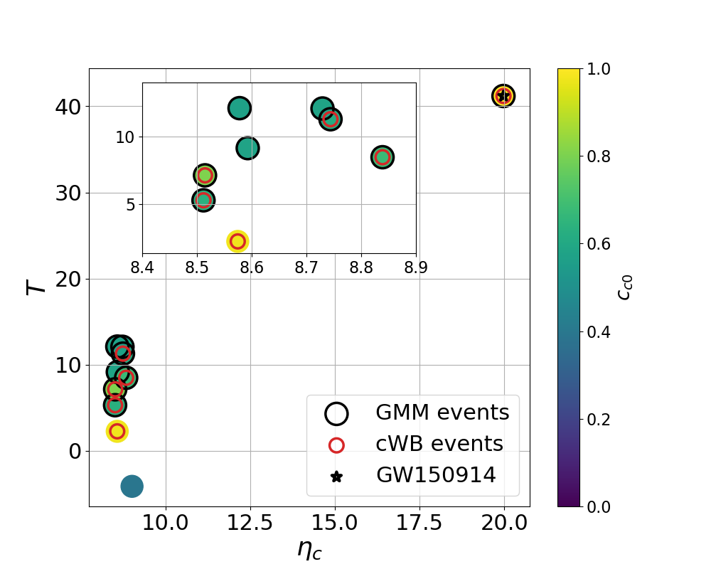
Figure 4: The network coherent SNR $\eta_{c}$ vs the GMM detection statistic $T$, with color corresponding to $c_{c0}$ for all 10 cWB triggers. Large black hollow circles correspond to detected cWB with GMM events (with $T>2.5$ equivelent to IFAR$>15$years) and smaller red hollow circles correspond to the standard-cWB events. The black star corresponds to the GW150914 event

V Conclusion

Detection of transient GWs in non-stationary and non-Gaussian noise poses a massive challenge in the advanced laser interferometric gravitational wave detectors. A number of approaches are used to combat spurious noisy triggers and to allow the detection of astrophysical GW transients with high significance. The standard-cWB GW burst search first makes a list of triggers – interesting time instances which could be either potential GW signals or background noise transients – and then applies a list of thresholds on the attributes to reject the noisy triggers. Although this thresholding approach is guided by extensive simulations and hence is largely successful, it is still ad-hoc in nature and relies on analysts intuition to optimise the thresholding process. In this work, we propose a supervised machine learning method using GMMs trained on cWB triggers. This training is applied using the O1 all-sky search triggers from the cWB search for short duration GW bursts to develop two distinct models for noise triggers and astrophysical GW burst triggers. We use these models to construct a log-likelihood based test statistic. We demonstrate that this approach gives improved performance as compared to the standard-cWB approach by improved signal detection probability at any FAR. We also obtain a significantly improved detection significance for GW150914 (the first ever GW merger event) with the cWB plus GMM detection approach. With this example, we clearly demonstrate that our more systematic GMM based signal detection approach can improve the detection performance as compared to the thresholding approach in the multi-dimensional attribute space.

It is worth noting that, like most GW search algorithms, the GMM approach is sensitive to simulation parameters used to train the signal model. Here, for comparison with standard-cWB, we have used the population of simulated signals that were generated for the O1 all-sky short duration burst search. The simulated data set was designed to provide an estimate of the search sensitivity to an ad-hoc population of signals and was not drawn from an astrophysical population. For example, the simulated data did not uniformly span the frequency band of the detectors. If we had included frequency as one of the parameters for the GMM, then the resulting test statistic would favour signals with frequencies corresponding to the simulated population which is not a desirable feature for unmodelled burst searches.

By applying the GMM to cWB trigger attributes, we are relying on cWB to efficiently capture all characteristics of an interesting event in these attributes. The cWB algorithm has undergone almost two decades of development and much effort has been put into the development and characterisation of the algorithm. Nonetheless, it may be possible to find more efficient ways to encode GW data for more effective GMM signal and noise model construction. For example, neural networks can be used to map GW strain data into a reduced number of parameters which are then used as inputs into the corresponding GMM.

In the near term, we plan to test this GMM approach using data from the second advanced detector observing run which contains a large variety of noisy triggers. The method is general enough and is not limited to short duration bursts triggers. We plan to extend this approach to GW searches for intermediate mass binary black hole mergers as such signals can be very difficult to distinguish from spurious noise transients, especially with increasing black hole mass.

VI Acknowledgements

The authors thank F. Salemi for useful comments. VG acknowledges Inspire division, DST, Government of India for the fellowship support. VG acknowledges support from the University of Florida. DL and RP thank Newton-Bhabha fund for the travel support to visit the University of Glasgow. AP acknowledges support from the SERB Matrics grant MTR/2019/001096 as well as the IIT-Bombay SEED grant for the travel funds to host the visit of ISH and CM to IIT Bombay. CM and ISH are supported by the Science and Technology Research Council (grant No. ST/ L000946/1) and the European Cooperation in Science and Technology (COST) action CA17137.

Appendix A Analytical Maximization of log likelihood

Here, we analytically maximize the log-likelihood function given in Eq. 4 under the constraint of $\sum_{j=1}^{K}w_{j}=1$. To estimate the weights $w_{1},w_{2},\dots,w_{K}$, we apply the method of Lagrange multipliers. Thus, we maximize

$$\mathcal{L}^{\prime} =\ln(p(X|\bm{\Theta}))+\lambda\left(\sum_{j=1}^{K}w_{j}-1\right)$$ (11)

with respect to $w_{k}$. This gives,

$$\frac{\partial\mathcal{L}^{\prime}}{\partial w_{k}}=\sum_{i=1}^{n}\frac{\mathcal{N}\left(\vec{x}_{i}|\boldsymbol{\mu_{k}},\Sigma_{k}\right)}{\sum_{j=1}^{K}w_{j}\mathcal{N}\left(\vec{x}_{i}|\boldsymbol{\mu_{k}},\Sigma_{k}\right)}+\lambda=0$$ (12)

Multiplying the above equation by $w_{k}$ and summing over $k$ we get,

$$\sum_{i=1}^{n}\frac{\sum_{k=1}^{K}w_{k}\mathcal{N}\left(\vec{x}_{i}|\boldsymbol{\mu_{k}},\Sigma_{k}\right)}{\sum_{j=1}^{K}w_{j}\mathcal{N}\left(\vec{x}_{i}|\boldsymbol{\mu_{k}},\Sigma_{k}\right)}+\lambda\sum_{k=1}^{K}w_{k}=0.$$

Summing over $i$ we obtain $\lambda=-n$. Substituting $\lambda$ in Eq. (12) and multiplying by $w_{k}$ we obtain,

$$nw_{k} =\sum_{i=1}^{n}r_{ik}\Rightarrow w_{k}=\frac{N_{k}}{n}$$ (13)

Therefore, the weight $w_{k}$ for the $k^{\text{th}}$ Gaussian component is given by the the average contribution of $N_{k}$.

References

- Abbott et al. (2017a) B. P. Abbott et al. (LIGO Scientific Collaboration, Virgo Collaboration), Phys. Rev. Lett. 119, 141101 (2017a), arXiv:1709.09660 [gr-qc] .
- Aasi et al. (2015) J. Aasi et al. (LIGO Scientific Collaboration), Class. Quant. Grav. 32, 074001 (2015), arXiv:1411.4547 [gr-qc] .
- Acernese et al. (2015) F. Acernese et al. (VIRGO), Class. Quant. Grav. 32, 024001 (2015), arXiv:1408.3978 [gr-qc] .
- Abbott et al. (2016a) B. P. Abbott et al. (LIGO Scientific Collaboration, Virgo Collaboration), Phys. Rev. Lett. 116, 061102 (2016a), arXiv:1602.03837 [gr-qc] .
- Abbott et al. (2016b) B. P. Abbott et al. (LIGO Scientific Collaboration, Virgo Collaboration), Phys. Rev. Lett. 116, 241103 (2016b), arXiv:1606.04855 [gr-qc] .
- Abbott et al. (2017b) B. P. Abbott et al. (LIGO Scientific Collaboration, Virgo Collaboration), Phys. Rev. Lett. 118, 221101 (2017b), arXiv:1706.01812 [gr-qc] .
- Abbott et al. (2017c) B. P. Abbott et al. (LIGO Scientific Collaboration, Virgo Collaboration), Astrophys. J. 851, L35 (2017c), arXiv:1711.05578 [astro-ph.HE] .
- Abbott et al. (2016c) B. P. Abbott et al. (LIGO Scientific Collaboration, Virgo Collaboration), Phys. Rev. X6, 041015 (2016c), [erratum: Phys. Rev.X8,no.3,039903(2018)], arXiv:1606.04856 [gr-qc] .
- Abbott et al. (2018) B. P. Abbott et al. (LIGO Scientific Collaboration and Virgo Collaboration), (2018), arXiv:1811.12907 [astro-ph.HE] .
- Abbott et al. (2017d) B. Abbott et al. (LIGO Scientific Collaboration, Virgo Collaboration), Phys. Rev. Lett. 119, 161101 (2017d), arXiv:1710.05832 [gr-qc] .
- Abbott et al. (2020) B. P. Abbott et al. (LIGO Scientific, Virgo), (2020), arXiv:2001.01761 [astro-ph.HE] .
- Aso et al. (2013) Y. Aso, Y. Michimura, K. Somiya, M. Ando, O. Miyakawa, T. Sekiguchi, D. Tatsumi, and H. Yamamoto (The KAGRA Collaboration), Phys. Rev. D88, 043007 (2013), arXiv:1306.6747 [gr-qc] .
- Iyer et al. (2011) B. Iyer et al., LIGO India Technical Document https://dcc.ligo.org/LIGO-M1100296/public (2011).
- Davis et al. (2020) D. Davis, L. V. White, and P. R. Saulson, (2020), arXiv:2002.09429 [gr-qc] .
- Abbott et al. (2016d) B. P. Abbott et al. (LIGO Scientific, Virgo), Class. Quant. Grav. 33, 134001 (2016d), arXiv:1602.03844 [gr-qc] .
- Nuttall et al. (2015) L. K. Nuttall, T. J. Massinger, J. Areeda, J. Betzwieser, S. Dwyer, A. Effler, R. P. Fisher, P. Fritschel, J. S. Kissel, A. P. Lundgren, D. M. Macleod, D. Martynov, J. McIver, A. Mullavey, D. Sigg, J. R. Smith, G. Vajente, A. R. Williamson, and C. C. Wipf, Classical and Quantum Gravity 32, 245005 (2015).
- Allen (2005) B. Allen, Phys. Rev. D71, 062001 (2005), arXiv:gr-qc/0405045 [gr-qc] .
- Nitz (2018) A. H. Nitz, Class. Quant. Grav. 35, 035016 (2018), arXiv:1709.08974 [gr-qc] .
- Dal Canton et al. (2014) T. Dal Canton, S. Bhagwat, S. Dhurandhar, and A. Lundgren, Class.Quant.Grav. 31, 015016 (2014), arXiv:1304.0008 [gr-qc] .
- Gayathri et al. (2019) V. Gayathri, P. Bacon, A. Pai, E. Chassande-Mottin, F. Salemi, and G. Vedovato, Phys. Rev. D 100, 124022 (2019).
- Bahaadini et al. (2018) S. Bahaadini, V. Noroozi, N. Rohani, S. Coughlin, M. Zevin, J. Smith, V. Kalogera, and A. Katsaggelos, Information Sciences 444, 172 (2018).
- Mukund et al. (2017) N. Mukund, S. Abraham, S. Kandhasamy, S. Mitra, and N. S. Philip, Phys. Rev. D 95, 104059 (2017).
- Colgan et al. (2020) R. E. Colgan, K. R. Corley, Y. Lau, I. Bartos, J. N. Wright, Z. Marka, and S. Marka, Phys. Rev. D 101, 102003 (2020), arXiv:1911.11831 [astro-ph.IM] .
- Cuoco et al. (2020) E. Cuoco et al., (2020), arXiv:2005.03745 [astro-ph.HE] .
- Vajente et al. (2020) G. Vajente, Y. Huang, M. Isi, J. C. Driggers, J. S. Kissel, M. J. Szczepańczyk, and S. Vitale, Phys. Rev. D 101, 042003 (2020).
- George and Huerta (2018) D. George and E. A. Huerta, Phys. Lett. B778, 64 (2018), arXiv:1711.03121 [gr-qc] .
- Gebhard et al. (2019) T. D. Gebhard, N. Kilbertus, and I. Harry, Phys. Rev. D 100, 063015 (2019), Phys. Rev. D100, 063015 (2019), arXiv:1904.08693 [astro-ph.IM] .
- Gabbard et al. (2019) H. Gabbard, C. Messenger, I. S. Heng, F. Tonolini, and R. Murray-Smith, (2019), arXiv:1909.06296 [astro-ph.IM] .
- Dempster et al. (1977) A. P. Dempster, N. M. Laird, and D. B. Rubin, Journal of the Royal Statistical Society: Series B (Methodological) 39, 1 (1977), https://rss.onlinelibrary.wiley.com/doi/pdf/10.1111/j.2517-6161.1977.tb01600.x .
- Klimenko et al. (2008) S. Klimenko, I. Yakushin, A. Mercer, and G. Mitselmakher, Class. Quant. Grav. 25, 114029 (2008), arXiv:0802.3232 [gr-qc] .
- Klimenko et al. (2005) S. Klimenko et al., Physical Review D 72, 122002 (2005), gr-qc/0508068 .
- Klimenko et al. (2016) S. Klimenko et al., Phys. Rev. D93, 042004 (2016), arXiv:1511.05999 [gr-qc] .
- Necula et al. (2012) V. Necula et al., Journal of Physics Conference Series 363, 012032 (2012).
- Abbott et al. (2017e) B. P. Abbott et al. (LIGO Scientific Collaboration and Virgo Collaboration), Phys. Rev. D95, 042003 (2017e), arXiv:1611.02972 [gr-qc] .