On Solving a Class of Fractional Semi-infinite Polynomial Programming Problems

Abstract.

In this paper, we study a class of fractional semi-infinite polynomial programming (FSIPP) problems, in which the objective is a fraction of a convex polynomial and a concave polynomial, and the constraints consist of infinitely many convex polynomial inequalities. To solve such a problem, we first reformulate it to a pair of primal and dual conic optimization problems, which reduce to semidefinite programming (SDP) problems if we can bring sum-of-squares structures into the conic constraints. To this end, we provide a characteristic cone constraint qualification for convex semi-infinite programming problems to guarantee strong duality and also the attainment of the solution in the dual problem, which is of its own interest. In this framework, we first present a hierarchy of SDP relaxations with asymptotic convergence for the FSIPP problem whose index set is defined by finitely many polynomial inequalities. Next, we study four cases of the FSIPP problems which can be reduced to either a single SDP problem or a finite sequence of SDP problems, where at least one minimizer can be extracted. Then, we apply this approach to the four corresponding multi-objective cases to find efficient solutions.

1. Introduction

In this paper, we consider the fractional semi-infinite polynomial programming (FSIPP) problem in the following form:

$$\left\{\begin{aligned} r^{\star}:=\min_{x\in{\mathbb{R}}^{m}}&\ \frac{f(x)}{g(x)}\\ \text{s.t.}&\ \psi_{1}(x)\leq 0,\ldots,\psi_{s}(x)\leq 0,\\ &\ p(x,y)\leq 0,\ \ \forall y\in\mathbf{Y}\subset{\mathbb{R}}^{n},\end{aligned}\right.$$ (1)

where $f,g$, $\psi_{1},\ldots,\psi_{s}\in{\mathbb{R}}[x]$ and $p\in{\mathbb{R}}[x,y]$. Here, ${\mathbb{R}}[x]$ (resp. ${\mathbb{R}}[x,y]$) denotes the ring of real polynomials in $x=(x_{1},\ldots,x_{m})$ (resp., $x=(x_{1},\ldots,x_{m})$ and $y=(y_{1},\ldots,y_{n})$). Denote by $\mathbf{K}$ and $\mathbf{S}$ the feasible set and the optimal solution set of (1), respectively. In this paper, we assume that $\mathbf{S}\neq\emptyset$ and make the following assumptions on (1):

(A1): $\mathbf{Y}$ is compact; $f$, $-g$, each $\psi_{i}$ and $p(\cdot,y)$ for each $y\in\mathbf{Y}$ are all convex in $x$;
(A2): Either $f(x)\geq 0$ and $g(x)>0$ for all $x\in\mathbf{K}$; or $g(x)$ is affine and $g(x)>0$ for all $x\in\mathbf{K}.$

The feasible set $\mathbf{K}$ is convex by (A1), while the objective of (1) is generally not convex. The assumption (A2) ensures that the objective of (1) is well-defined. It is commonly adopted in the literature about fractional optimization problems [24, 36, 44], and can be satisfied by many practical optimization models [4, 36, 49]. If $\mathbf{Y}$ is noncompact, the technique of homogenization can be applied (c.f. [53]).

Over the last several decades, due to a great number of applications in many fields, semi-infinite programming (SIP) has attracted a great interest and has been a very active research area [14, 15, 22, 35]. Numerically, SIP problems can be solved by different approaches including, for instance, discretization methods, local reduction methods, exchange methods, simplex-like methods, feasible point methods etc; see [14, 22, 35] and the references therein for details. A main difficulties in solving general SIP problems is that the feasibility test of a given point is equivalent to globally solving a lower level subproblem which is generally nonlinear and nonconvex.

To the best of our knowledge, there are only limited research results devoted to semi-infinite polynomial optimization by exploiting features of polynomial optimization problems. For instance, Parpas and Rustem [40] proposed a discretization-like method to solve minimax polynomial optimization problems, which can be reformulated as semi-infinite polynomial programming (SIPP) problems. Using polynomial approximation and an appropriate hierarchy of semidefinite programming (SDP) relaxations, Lasserre [29] presented an algorithm to solve the generalized SIPP problems. Based on an exchange scheme, an SDP relaxation method for solving SIPP problems was proposed in [53]. By using representations of nonnegative polynomials in the univariate case, an SDP method was given in [54] for linear SIPP problems with the index set being closed intervals. For convex SIPP problems, Guo and Sun [16] proposed an SDP relaxation method by combining the sum-of-squares representation of the Lagrangian function with high degree perturbations [30] and Putinar’s representation [42] of the constraint polynomial on the index set.

In this paper, in a way similar to [16], we will derive an SDP relaxation method for the FSIPP problem (1). Different from [16], we treat the problem in a more systematical manner. We first reformulate the FSIPP problem to a conic optimization problem and its Lagrangian dual, which involve two convex cones of polynomials in the variables and the parameters, respectively (Section 3). Under suitable assumptions on these cones, approximate minimum and minimizers of the FSIPP problem can be obtained by solving the conic reformulations. If we can bring sum-of-squares structures into these cones, the conic reformulations reduce to a pair of SDP problems and become tractable. To this end, inspired by Jeyakumar and Li [23], we provide a characteristic cone constraint qualification for convex semi-infinite programming problems to guarantee the strong duality and the attachment of the solution in the dual problem, which is of its own interest. We remark that this constraint qualification, which is crucial for some applications (see Section 5.2), is weaker than the Slater condition used in [16].

In what follows, we first present a hierarchy of SDP relaxations for the FSIPP problem whose index set is defined by finitely many polynomial inequalities (Section 4). This is done by introducing appropriate quadratic modules to the conic reformulations. The asymptotic convergence of the optimal values of the SDP relaxations to the minimum of the FSIPP problem can be established by Putinar’s Positivstellensatz [42]. Moreover, when the FSIPP problem has a unique minimizer, this minimizer can be approximated from the optimal solutions to the SDP relaxations. By means of existing complexity results of Putinar’s Positivstellensatz, we can derive some convergence rate analysis of the SDP relaxations. We also present some discussions on the stop criterion for such SDP relaxations. Next, we restrict our focus on four cases of FSIPP problems for which the SDP relaxation method is exact or has finite convergence and at least one minimizer can be extracted (Section 5). The reason for this restriction is due to some applications of the FSIPP problem where exact minimum and minimizers are required. In particular, we study the application of our SDP method to the corresponding multi-objective FSIPP problems, where the objective function is a vector valued function with each component being a fractional function. We aim to find efficient solutions (see Definition 5.1) to such problems. Some sufficient efficiency conditions and duality results for such problems can be found in [8, 52, 55, 56]. However, as far as we know, very few algorithmic developments are available for such problems in the literature because of the difficulty of checking feasibility of a given point.

This paper is organized as follows. Some notation and preliminaries are given in Section 2. The FSIPP problem is reformulated as a conic optimization problem in Section 3. We present a hierarchy of SDP relaxations for FSIPP problems in Section 4. In Section 5, we consider four specified cases of the FSIPP problems and the application of the SDP method to the multi-objective cases. Some conclusions are given in Section 6.

2. Notation and Preliminaries

In this section, we collect some notation and preliminary results which will be used in this paper. The symbol $\mathbb{N}$ (resp., $\mathbb{R}$, ${\mathbb{R}}_{+}$) denotes the set of nonnegative integers (resp., real numbers, nonnegative real numbers). For any $t\in\mathbb{R}$, $\lceil t\rceil$ denotes the smallest integer that is not smaller than $t$. For $u\in\mathbb{R}^{m}$, $\|u\|$ denotes the standard Euclidean norm of $u$. For $\alpha=(\alpha_{1},\ldots,\alpha_{n})\in\mathbb{N}^{n}$, $|\alpha|=\alpha_{1}+\cdots+\alpha_{n}$. For $k\in\mathbb{N}$, denote $\mathbb{N}^{n}_{k}=\{\alpha\in\mathbb{N}^{n}\mid|\alpha|\leq k\}$ and $|\mathbb{N}^{n}_{k}|$ its cardinality. For variables $x\in\mathbb{R}^{m}$, $y\in\mathbb{R}^{n}$ and $\beta\in\mathbb{N}^{m},\alpha\in\mathbb{N}^{n}$, $x^{\beta}$, $y^{\alpha}$ denote $x_{1}^{\beta_{1}}\cdots x_{m}^{\beta_{m}}$, $y_{1}^{\alpha_{1}}\cdots y_{n}^{\alpha_{n}}$, respectively. For $h\in{\mathbb{R}}[x]$, we denote by $\deg(h)$ its (total) degree. For $k\in\mathbb{N}$, denote by ${\mathbb{R}}[x]_{k}$ (resp., ${\mathbb{R}}[y]_{k}$) the set of polynomials in ${\mathbb{R}}[x]$ (resp., ${\mathbb{R}}[y]$) of degree up to $k$. For $A={\mathbb{R}}[x],\ {\mathbb{R}}[y],\ {\mathbb{R}}[x]_{k},\ {\mathbb{R}}[y]_{k}$, denote by $A^{*}$ the dual space of linear functionals from $A$ to ${\mathbb{R}}$.

A polynomial $h\in{\mathbb{R}}[x]$ is said to be a sum-of-squares (s.o.s) of polynomials if it can be written as $h=\sum_{i=1}^{l}h_{i}^{2}$ for some $h_{1},\ldots,h_{l}\in{\mathbb{R}}[x]$. The symbols $\Sigma^{2}[x]$ and $\Sigma^{2}[y]$ denote the sets of polynomials that are s.o.s in ${\mathbb{R}}[x]$ and ${\mathbb{R}}[y]$, respectively. Notice that not every nonnegative polynomial can be written as s.o.s, see [43]. We recall the following properties about polynomials nonnegative on certain sets, which will be used in this paper.

Theorem 2.1 (Hilbert’s theorem).

Every nonnegative polynomial $h\in{\mathbb{R}}[x]$ can be written as s.o.s in the following cases: (i) $m=1$; (ii) $\deg(h)=2$; (iii) $m=2$ and $\deg(h)=4$.

Theorem 2.2 (The $S$-lemma).

Let $h,$ $q\in{\mathbb{R}}[x]$ be two quadratic polynomials and assume that there exists $u^{0}\in{\mathbb{R}}^{m}$ with $q(u^{0})>0$. The following assertions are equivalent: (i) $q(x)\geq 0$ $\Rightarrow$ $h(x)\geq 0$; (ii) there exists $\lambda\geq 0$ such that $h(x)\geq\lambda q(x)$ for all $x\in{\mathbb{R}}^{m}$.

Proposition 2.1.

[45, Example 3.18] Let $q\in{\mathbb{R}}[x]$ and the set $\mathcal{K}=\{x\in{\mathbb{R}}^{m}\mid q(x)\geq 0\}$ be compact. If $h\in{\mathbb{R}}[x]$ is nonnegative on $\mathcal{K}$ and the following conditions hold

1. $h$ has only finitely many zeros on $\mathcal{K},$ each lying in the interior of $\mathcal{K};$

2. the Hessian $\nabla^{2}h$ is positive definite on each of these zeros,

then $h=\sigma_{0}+\sigma_{1}q$ for some $\sigma_{0},\sigma_{1}\in\Sigma^{2}[x]$.

For $h,h_{1},\ldots,h_{\kappa}\in{\mathbb{R}}[x]$, let us recall some background about Lasserre’s hierarchy [27] for the polynomial optimization problem

$$h^{\star}:=\min_{x\in{\mathbb{R}}^{m}}\ h(x)\quad\text{s.t.}\quad x\in S:=\{x\in{\mathbb{R}}^{m}\mid h_{1}(x)\geq 0,\ldots,h_{\kappa}(x)\geq 0\}\not=\emptyset.$$ (2)

Let $H:=\{h_{1},\ldots,h_{\kappa}\}$ and $h_{0}=1$ for convenience. We denote by

$$\mathbf{qmodule}(H):=\left\{\sum_{j=0}^{\kappa}h_{j}\sigma_{j}\ \Big{|}\ \sigma_{j}\in\Sigma^{2}[x],j=0,1,\ldots,\kappa\right\}$$

the quadratic module generated by $H$ and denote by

$$\mathbf{qmodule}_{k}(H):=\left\{\sum_{j=0}^{\kappa}h_{j}\sigma_{j}\ \Big{|}\ \sigma_{j}\in\Sigma^{2}[x],\,\deg(h_{j}\sigma_{j})\leq 2k,\ j=0,1,\ldots,\kappa\right\}$$

its $k$-th quadratic module. It is clear that if $h\in\mathbf{qmodule}(H)$, then $h(x)\geq 0$ for any $x\in S$. However, the converse is not necessarily true.

Definition 2.1.

We say that $\mathbf{qmodule}(H)$ is Archimedean if there exists $\phi\in\mathbf{qmodule}(H)$ such that the inequality $\phi(x)\geq 0$ defines a compact set in ${\mathbb{R}}^{m};$ or equivalently, if for all $\phi\in{\mathbb{R}}[x],$ there is some $N\in\mathbb{N}$ such that $N\pm\phi\in\mathbf{qmodule}(H)$ $($c.f., [46]$)$.

Note that for any compact set $S$ we can always force the associated quadratic module to be Archimedean by adding a redundant constraint $M-\|x\|^{2}_{2}\geq 0$ in the description of $S$ for a sufficiently large $M$.

Theorem 2.3.

[42, Putinar’s Positivstellensatz] Suppose that $\mathbf{qmodule}(H)$ is Archimedean. If a polynomial $\psi\in{\mathbb{R}}[x]$ is positive on $S,$ then $\psi\in\mathbf{qmodule}_{k}(H)$ for some $k\in\mathbb{N}$.

For a polynomial $\psi(x)=\sum_{\alpha\in\mathbb{N}^{m}}\psi_{\alpha}x^{\alpha}\in{\mathbb{R}}[x]$ where $\psi_{\alpha}$ denotes the coefficient of the monomial $x^{\alpha}$ in $\psi$, define the norm

$$\|\psi\|:=\max_{\alpha\in\mathbb{N}^{m}}\frac{|\psi_{\alpha}|}{\tbinom{|\alpha|}{\alpha}}.$$ (3)

We have the following result for an estimation of the order $k$ in Theorem 2.3.

Theorem 2.4.

[39, Theorem 6] Suppose that $\mathbf{qmodule}(H)$ is Archimedean and $S\subseteq(-\tau_{S},\tau_{S})^{m}$ for some $\tau_{S}>0$. Then there is some positive $c\in{\mathbb{R}}$ $($depending only on $h_{j}$’s$)$ such that for all $\psi\in{\mathbb{R}}[x]$ of degree $d$ with $\min_{x\in S}\psi(x)>0,$ we have $\psi\in\mathbf{qmodule}_{k}(H)$ whenever

$$k\geq c\exp\left[\left(d^{2}m^{d}\frac{\|\psi\|\tau_{S}^{d}}{\min_{x\in S}\psi(x)}\right)^{c}\right].$$

For an integer $k\geq\max\{\lceil\deg(h)/2\rceil,k_{0}\}$ where $k_{0}:=\max\{\lceil\deg(h_{i})/2\rceil,i=1,\ldots,\kappa\}$, the $k$-th Lasserre’s relaxation for (2) is

$$h_{k}^{\mbox{\tiny dual}}:=\inf_{\mathscr{L}}\ \mathscr{L}(h)\ \ \text{s.t.}\ \ \mathscr{L}\in(\mathbf{qmodule}_{k}(H))^{*},\ \mathscr{L}(1)=1,$$ (4)

and its dual problem is

$$h_{k}^{\mbox{\tiny primal}}:=\sup_{\rho}\ \rho\ \ \text{s.t.}\ \ h-\rho\in\mathbf{qmodule}_{k}(H).$$ (5)

For each $k\geq k_{0}$, (4) and (5) can be reduced to a pair of primal and dual SDP problems, and we always have $h_{k}^{\mbox{\tiny primal}}\leq h_{k}^{\mbox{\tiny dual}}\leq h^{\star}$ (c.f. [27]). The convergence of $h_{k}^{\mbox{\tiny dual}}$ and $h_{k}^{\mbox{\tiny primal}}$ to $h^{\star}$ as $k\rightarrow\infty$ can be established by Putinar’s Positivstellensatz [27, 42] under the Archimedean condition. If there exists an integer $k^{\star}$ such that $h_{k}^{\mbox{\tiny primal}}=h_{k}^{\mbox{\tiny dual}}=h^{\star}$ for each $k\geq k^{\star}$, we say that Lasserre’s hierarchy for (2) has finite convergence. To certify $h_{k}^{\mbox{\tiny dual}}=h^{\star}$ when it occurs, a sufficient condition on a minimizer of (4) called flat extension condition [9] is available. A weaker condition called flat truncation condition was proposed by Nie in [37]. Precisely, for a linear functional $\mathscr{L}\in({\mathbb{R}}[x]_{2k})^{*}$, denote by $\mathbf{M}_{k}(\mathscr{L})$ the associated $k$-th moment matrix which is indexed by $\mathbb{N}^{m}_{k}$, with $(\alpha,\beta)$-th entry being $\mathscr{L}(x^{\alpha+\beta})$ for $\alpha,\beta\in\mathbb{N}^{m}_{k}$.

Condition 2.1.

[37, flat truncation condition] A minimizer $\mathscr{L}^{\star}\in({\mathbb{R}}[x]_{2k})^{*}$ of (4) satisfies the following rank condition$:$ there exists an integer $k^{\prime}$ with $\max\{\lceil\deg(h)/2\rceil,k_{0}\}\leq k^{\prime}\leq k$ such that

$$\mbox{rank}\ \mathbf{M}_{k^{\prime}-k_{0}}(\mathscr{L}^{\star})=\mbox{rank}\ \mathbf{M}_{k^{\prime}}(\mathscr{L}^{\star}).$$

Nie [37, Theorem 2.2] proved that Lasserre’s hierarchy has finite convergence if and only if the flat truncation holds, under some generic assumptions. In particular, we have the following proposition.

Proposition 2.2.

[37, c.f. Theorem 2.2] Suppose that the set $\{x\in{\mathbb{R}}^{m}\mid h(x)=h^{\star}\}$ is finite, the set of global minimizers of (2) is nonempty, and for $k$ big enough the optimal value of (5) is achievable and there is no duality gap between (4) and (5). Then, for $k$ sufficiently large, $h_{k}^{\mbox{\tiny primal}}=h_{k}^{\mbox{\tiny dual}}=h^{\star}$ if and only if every minimizer of (4) satisfies the flat truncation condition.

Moreover, if a minimizer $\mathscr{L}^{\star}\in({\mathbb{R}}[x]_{2k})^{*}$ of (2) satisfies the flat extension condition or the flat truncation condition, we can extract finitely many global minimizers of (2) from the moment matrix $\mathbf{M}_{k}(\mathscr{L}^{\star})$ by solving a linear algebra problem (c.f. [9, 20]). Such procedure has been implemented in the software GloptiPoly [21] developed by Henrion, Lasserre and Löfberg.

We say that a linear functional $\mathscr{L}\in({\mathbb{R}}[x])^{*}$ has a representing measure $\mu$ if there exists a Borel measure $\mu$ on ${\mathbb{R}}^{m}$ such that

$$\mathscr{L}(x^{\alpha})=\int_{{\mathbb{R}}^{m}}x^{\alpha}\mathrm{d}\mu(x),\quad\forall\alpha\in\mathbb{N}^{m}.$$

For $k\in\mathbb{N}$, we say that $\mathscr{L}\in({\mathbb{R}}[x]_{k})^{*}$ has a representing measure $\mu$ if the above holds for all $\alpha\in\mathbb{N}^{m}_{k}$. By [9, Theorem 1.1], Condition 2.1 implies that $\mathscr{L}^{\star}$ has an atomic representing measure. Each atom of the measure is a global minimizer of (2) and can be extracted by the procedure presented in [20].

We end this section by introducing some important properties on convex polynomials.

Definition 2.2.

A polynomial $h\in{\mathbb{R}}[x]$ is coercive whenever the lower level set $\{x\in{\mathbb{R}}^{m}\mid h(x)\leq\alpha\}$ is a $($possibly empty$)$ compact set, for all $\alpha\in{\mathbb{R}}$.

Proposition 2.3.

[25, Lemma 3.1] Let $h\in{\mathbb{R}}[x]$ be a convex polynomial. If $\nabla^{2}h(u^{\prime})\succ 0$ at some point $u^{\prime}\in{\mathbb{R}}^{m},$ then $h$ is coercive and strictly convex on ${\mathbb{R}}^{m}.$

Recall also a subclass of convex polynomials in ${\mathbb{R}}[x]$ introduced by Helton and Nie [19].

Definition 2.3.

[19] A polynomial $h\in{\mathbb{R}}[x]$ is s.o.s-convex if its Hessian $\nabla^{2}h$ is an s.o.s-matrix, i.e., there is some integer $r$ and some matrix polynomial $H\in{\mathbb{R}}[x]^{r\times m}$ such that $\nabla^{2}h(x)=H(x)^{T}H(x)$.

In fact, Ahmadi and Parrilo [2] has proved that a convex polynomial $h\in{\mathbb{R}}[x]$ is s.o.s-convex if and only if $m=1$ or $\deg(h)=2$ or $(m,\deg(h))=(2,4)$. In particular, the class of s.o.s-convex polynomials contains the classes of separable convex polynomials and convex quadratic functions.

The significance of s.o.s-convexity is that it can be checked numerically by solving an SDP problem (see [19]), while checking the convexity of a polynomial is generally NP-hard (c.f. [1]). Interestingly, an extended Jensen’s inequality holds for s.o.s-convex polynomials.

Proposition 2.4.

[28, Theorem 2.6] Let $h\in{\mathbb{R}}[x]_{2d}$ be s.o.s-convex, and let $\mathscr{L}\in({\mathbb{R}}[x]_{2d})^{*}$ satisfy $\mathscr{L}(1)=1$ and $\mathscr{L}(\sigma)\geq 0$ for every $\sigma\in\Sigma^{2}[x]\cap{\mathbb{R}}[x]_{2d}$. Then,

$$\mathscr{L}(h(x))\geq h(\mathscr{L}(x_{1}),\ldots,\mathscr{L}(x_{m})).$$

The following result plays a significant role for the SDP relaxations of (1) in Section 5.

Lemma 2.1.

[19, Lemma 8] Let $h\in{\mathbb{R}}[x]$ be s.o.s-convex. If $h(u)=0$ and $\nabla h(u)=0$ for some $u\in{\mathbb{R}}^{m},$ then $h$ is an s.o.s polynonmial.

3. Conic reformulation of FSIPP

In this section, we first reformulate the FSIPP problem (1) to a conic optimization problem and its Lagrangian dual, which involve two convex subcones of ${\mathbb{R}}[x]$ and ${\mathbb{R}}[y]$, respectively. Under suitable assumptions on these cones, we show that approximate minimum and minimizers of (1) can be obtained by solving the conic reformulations.

3.1. Problem Reformulation

Consider the problem

$$\min_{x\in\mathbf{K}}\ \ f(x)-r^{\star}g(x).$$ (6)

Note that, under (A1-2), (6) is clearly a convex semi-infinite programming problem and its optimal value is $0$.

Now we consider the Lagrangian dual of (6). In particular, the constraints $p(x,y)\leq 0$ for all $y\in\mathbf{Y}$ means that for each $u\in\mathbf{K}$, $p(u,y)\in{\mathbb{R}}[y]$ belongs to the cone of nonpositive polynomials on $\mathbf{Y}$. The polar of this cone is taken as the cone of finite nonnegative measures supported on $\mathbf{Y}$, which we denote by $\mathcal{M}(\mathbf{Y})$. Therefore, we can define the Lagrangian function $L_{f,g}(x,\mu,\eta):{\mathbb{R}}^{m}\times\mathcal{M}(\mathbf{Y})\times{\mathbb{R}}_{+}^{s}\rightarrow{\mathbb{R}}$ by

$$L_{f,g}(x,\mu,\eta)=f(x)-r^{\star}g(x)+\int_{\mathbf{Y}}p(x,y)d\mu(y)+\sum_{j=1}^{s}\eta_{j}\psi_{j}(x).$$ (7)

Then, the Lagrangian dual of (6) reads

$$\max_{\mu\in\mathcal{M}(\mathbf{Y}),\eta_{j}\geq 0}\inf_{x\in{\mathbb{R}}^{m}}L_{f,g}(x,\mu,\eta).$$ (8)

See [7, 22, 35, 47] for more details.

Consider the strong duality and dual attainment for the dual pair (6) and (8):

(A3): $\exists\mu^{\star}\in\mathcal{M}(\mathbf{Y})$ and $\eta^{\star}\in{\mathbb{R}}_{+}^{s}$ such that $\inf_{x\in{\mathbb{R}}^{m}}L_{f,g}(x,\mu^{\star},\eta^{\star})=0$.

The following straightforward result is essential for the SDP relaxations of (1) in Section 5.

Proposition 3.1.

Under (A1-3), $L_{f,g}(u^{\star},\mu^{\star},\eta^{\star})=0$ and $\nabla_{x}L_{f,g}(u^{\star},\mu^{\star},\eta^{\star})=0$ for any $u^{\star}\in\mathbf{S}$.

Under (A1-3), we first reformulate (1) to a conic optimization problem with the same optimal value $r^{\star}$. We need the following notation. For a subset $\mathcal{X}\subset{\mathbb{R}}^{m}$ (resp., the index set $\mathbf{Y}$), denote by $\mathscr{P}(\mathcal{X})\subset{\mathbb{R}}[x]$ (resp. $\mathscr{P}(\mathbf{Y})\subset{\mathbb{R}}[y]$) the cone of nonnegative polynomials on $\mathcal{X}$ (resp., $\mathbf{Y}$). For $\mathscr{L}\in({\mathbb{R}}[x])^{*}$ (resp., $\mathscr{H}\in({\mathbb{R}}[y])^{*}$), denote by $\mathscr{L}(p(x,y))$ (resp., $\mathscr{H}(p(x,y))$) the image of $\mathscr{L}$ (resp., $\mathscr{H}$) on $p(x,y)$ regarded as an element in ${\mathbb{R}}[x]$ (resp., ${\mathbb{R}}[y]$) with coefficients in ${\mathbb{R}}[y]$ (resp., ${\mathbb{R}}[x]$), i.e., $\mathscr{L}(p(x,y))\in{\mathbb{R}}[y]$ (resp., $\mathscr{H}(p(x,y)))\in{\mathbb{R}}[x]$). For a subset $\mathcal{X}\subset{\mathbb{R}}^{m}$, consider the conic optimization problem

$$\left\{\begin{aligned} \tilde{r}:=\sup_{\rho,\mathscr{H},\eta}\ &\rho&\\ \text{s.t.}\ &f(x)-\rho g(x)+\mathscr{H}(p(x,y))+\sum_{j=1}^{s}\eta_{j}\psi_{j}(x)\in\mathscr{P}(\mathcal{X}),&\\ &\rho\in{\mathbb{R}},\ \mathscr{H}\in(\mathscr{P}(\mathbf{Y}))^{*},\ \eta\in{\mathbb{R}}_{+}^{s}.&\end{aligned}\right.$$ (9)

Proposition 3.2.

Under (A1-3), suppose that $\mathcal{X}\cap\mathbf{S}\neq\emptyset$, then $\tilde{r}=r^{\star}$.

Proof.

Under (A3), define $\mathscr{H}^{\star}\in({\mathbb{R}}[y])^{*}$ by letting $\mathscr{H}^{\star}(y^{\beta})=\int_{\mathbf{Y}}y^{\beta}d\mu^{\star}(y)$ for any $\beta\in\mathbb{N}^{n}$. Then, $\mathscr{H}^{\star}\in(\mathscr{P}(\mathbf{Y}))^{*}$ and $(r^{\star},\mathscr{H}^{\star},\eta^{\star})$ is feasible to (9). Hence, $\tilde{r}\geq r^{\star}$. As $\mathcal{X}\cap\mathbf{S}\neq\emptyset$, for any $u^{\star}\in\mathcal{X}\cap\mathbf{S}$ and any $(\rho,\mathscr{H},\eta)$ feasible to (9), it holds that

$$f(u^{\star})-\rho g(u^{\star})+\mathscr{H}(p(u^{\star},y))+\sum_{j=1}^{s}\eta_{j}\psi_{j}(u^{\star})\geq 0.$$

Then, the feasibility of $u^{\star}$ to (1) implies that $r^{\star}=\frac{f(u^{\star})}{g(u^{\star})}\geq\rho$ and thus $r^{\star}\geq\tilde{r}$. ∎

Remark 3.1.

Before moving forward, let us give a brief overview on the strategies we adopted in this paper to construct SDP relaxations of (1) from the reformulation (9). The difficulty of (9) is that the exact representions of the convex cones $\mathscr{P}(\mathcal{X})$ and $\mathscr{P}(\mathbf{Y})$ are usually not available in general case, which makes (9) still intractable. However, the Positivstellensatz from real algebraic geometry, which provides algebraic certificates for positivity (nonnegative) of polynomials on semialgebraic sets, can gives us approximations of $\mathscr{P}(\mathcal{X})$ (with a carefully chosen $\mathcal{X}$) and $\mathscr{P}(\mathbf{Y})$ with sum-of-squares structures. Replacing $\mathscr{P}(\mathcal{X})$ and $\mathscr{P}(\mathbf{Y})$ by these approximations, we can convert (9) into SDP relaxations of (1). In order to obtain (approximate) optimum and optimizers of (1) from the resulting SDP relaxations, we need establish some conditions which should be satisfied by these approximations of $\mathscr{P}(\mathcal{X})$ and $\mathscr{P}(\mathbf{Y})$. Then according to these conditions, we can choose suitable subset $\mathcal{X}$ and construct appropriate approximations $\mathscr{P}(\mathcal{X})$ and $\mathscr{P}(\mathbf{Y})$. Remark that different subsets $\mathcal{X}$ and versions of Positivstellensatz can lead to different approximations of $\mathscr{P}(\mathcal{X})$ and $\mathscr{P}(\mathbf{Y})$ satisfying the established conditions. Therefore, to present our approach in a unified way, we next use the symbols $\mathcal{C}[x]$ and $\mathcal{C}[y]$ to denote approximations of $\mathscr{P}(\mathcal{X})$ and $\mathscr{P}(\mathbf{Y})$, respectively, and derive the conditions they should satisfy (Theorem 3.1). Then, we specify suitable $\mathcal{C}[x]$ and $\mathcal{C}[y]$ in different situations to construct concrete SDP relaxations of (1) in Section 4 and 5. ∎

Let $\mathcal{C}[x]$ (resp., $\mathcal{C}[y]$) be a convex cone in ${\mathbb{R}}[x]$ (resp., ${\mathbb{R}}[y]$). Replacing $\mathscr{P}(\mathcal{X})$ and $\mathscr{P}(\mathbf{Y})$ by $\mathcal{C}[x]$ and $\mathcal{C}[y]$ in (9), respectively, we get the conic optimization problem

$$\left\{\begin{aligned} r^{\mbox{\tiny primal}}:=\sup_{\rho,\mathscr{H},\eta}\ &\rho&\\ \text{s.t.}\ &f(x)-\rho g(x)+\mathscr{H}(p(x,y))+\sum_{j=1}^{s}\eta_{j}\psi_{j}(x)\in\mathcal{C}[x],&\\ &\rho\in{\mathbb{R}},\ \mathscr{H}\in(\mathcal{C}[y])^{*},\ \eta\in{\mathbb{R}}_{+}^{s},&\end{aligned}\right.$$ (10)

and its Lagrangian dual

$$\left\{\begin{aligned} r^{\mbox{\tiny dual}}:=\inf_{\mathscr{L}}\ &\mathscr{L}(f)&\\ \text{s.t.}\ &\mathscr{L}\in(\mathcal{C}[x])^{*},\ \mathscr{L}(g)=1,&\\ &-\mathscr{L}(p(x,y))\in\mathcal{C}[y],\ \mathscr{L}(\psi_{j})\leq 0,\ j=1,\ldots,s.&\end{aligned}\right.$$ (11)

For simplicity, in what follows, we adopt the notation

$$\mathscr{L}(x):=(\mathscr{L}(x_{1}),\ldots,\mathscr{L}(x_{m}))$$

for any $\mathscr{L}\in({\mathbb{R}}[x])^{*}$. Let

$$\mathbf{d}:=\max\{\deg(f),\deg(g),\deg(\psi_{1}),\ldots,\deg(\psi_{s}),\deg_{x}(p(x,y))\}.$$ (12)

For any $\varepsilon\geq 0$, denote the set of $\varepsilon$-optimal solutions of (1)

$$\mathbf{S}_{\varepsilon}:=\left\{x\in\mathbf{K}\ \Big{|}\ \frac{f(x)}{g(x)}\leq r^{\star}+\varepsilon\right\}.$$ (13)

The following results show that if the cones $\mathcal{C}[x]$ and $\mathcal{C}[y]$ satisfy certain conditions, we can approximate $r^{\star}$ and extract an $\varepsilon$-optimal solution by solving (10) and (11).

Theorem 3.1.

Suppose that (A1-2) hold and $\mathcal{C}[y]\subseteq\mathscr{P}(\mathbf{Y})$. For some $\varepsilon\geq 0,$ suppose that there exists some $u^{(\varepsilon)}\in\mathbf{S}_{\varepsilon}$ such that $-p(u^{(\varepsilon)},y)\in\mathcal{C}[y]$ and $h(u^{(\varepsilon)})\geq 0$ for any $h(x)\in\mathcal{C}[x]$.

1. If (A3) holds and $L_{f,g}(x,\mu^{\star},\eta^{\star})+\varepsilon g(x)\in\mathcal{C}[x]$, then $r^{\star}-\varepsilon\leq r^{\mbox{\tiny primal}}\leq r^{\mbox{\tiny dual}}\leq r^{\star}+\varepsilon$.

2. If $\mathscr{L}^{\star}$ is a minimizer of (11) such that the restriction $\mathscr{L}^{\star}|_{{\mathbb{R}}[x]_{\mathbf{d}}}$ admits a representing nonnegative measure $\nu,$ then $r^{\star}\leq r^{\mbox{\tiny dual}}\leq r^{\star}+\varepsilon$ and

   $$\frac{\mathscr{L}^{\star}(x)}{\mathscr{L}^{\star}(1)}=\frac{1}{\int d\nu}\left(\int x_{1}d\nu,\ldots,\int x_{m}d\nu\right)\in\mathbf{S}_{\varepsilon}.$$

Proof.

Define a linear functional $\mathscr{L}^{\prime}\in({\mathbb{R}}[x])^{*}$ such that $\mathscr{L}^{\prime}(x^{\alpha})=\frac{(u^{\varepsilon})^{\alpha}}{g(u^{\varepsilon})}$ for each $\alpha\in\mathbb{N}^{m}$. By the assumption, it is clear that $\mathscr{L}^{\prime}$ is feasible to (11). Then, $r^{\mbox{\tiny dual}}\leq\mathscr{L}^{\prime}(f)=\frac{f(u^{\varepsilon})}{g(u^{\varepsilon})}\leq r^{\star}+\varepsilon$.

(i) Define $\mathscr{H}^{\star}\in({\mathbb{R}}[y])^{*}$ by letting $\mathscr{H}^{\star}(y^{\beta})=\int_{\mathbf{Y}}y^{\beta}d\mu^{\star}(y)$ for any $\beta\in\mathbb{N}^{n}$. By the assumption, $\mathscr{H}^{\star}\in(\mathcal{C}[y])^{*}$. Since $L_{f,g}(x,\mu^{\star},\eta^{\star})+\varepsilon g(x)\in\mathcal{C}[x]$, $(r^{\star}-\varepsilon,\mathscr{H}^{\star},\eta^{\star})$ is feasible to (10). Hence, $r^{\mbox{\tiny primal}}\geq r^{\star}-\varepsilon$. Then, the weak duality implies the conclusion.

(ii) As $\mathscr{L}^{\star}|_{{\mathbb{R}}[x]_{\mathbf{d}}}$ admits a representing nonnegative measure $\nu$, we have $\mathscr{L}^{\star}(1)=\int d\nu>0$; otherwise $\mathscr{L}^{\star}(g)=0$, a contradiction. For every $y\in\mathbf{Y}$, as $p(x,y)$ is convex in $x$ and $\frac{\nu}{\int d\nu}$ is a probability measure, by Jensen’s inequality, we have

$$p\left(\frac{\mathscr{L}^{\star}(x)}{\mathscr{L}^{\star}(1)},y\right)\leq\frac{1}{\int d\nu}\int p(x,y)d\nu(x)=\frac{1}{\mathscr{L}^{\star}(1)}\mathscr{L}^{\star}(p(x,y))\leq 0,$$ (14)

where the last inequality follows from the constraint of the Lagrangian dual problem (11). For the same reason,

$$\psi_{j}\left(\frac{\mathscr{L}^{\star}(x)}{\mathscr{L}^{\star}(1)}\right)\leq 0,\ \ j=1,\ldots,s,$$ (15)

which implies that $\mathscr{L}^{\star}(x)/\mathscr{L}^{\star}(1)$ is feasible to (1). Therefore, it holds that

$$r^{\star}+\varepsilon \geq\mathscr{L}^{\star}(f)=\frac{\mathscr{L}^{\star}(f)}{\mathscr{L}^{\star}(g)}=\frac{\int f(x)d\nu}{\int g(x)d\nu}=\frac{\frac{1}{\int d\nu}\int f(x)d\nu}{\frac{1}{\int d\nu}\int g(x)d\nu}$$

$$\geq\frac{f\left(\mathscr{L}^{\star}(x)/\mathscr{L}^{\star}(1)\right)}{g(\mathscr{L}^{\star}(x)/\mathscr{L}^{\star}(1))}\geq r^{\star}.$$

In particular, the second inequality above can be easily verified under (A2). Therefore, we have $r^{\star}\leq r^{\mbox{\tiny dual}}\leq r^{\star}+\varepsilon$ and $\mathscr{L}^{\star}(x)/\mathscr{L}^{\star}(1)\in\mathbf{S}_{\varepsilon}$. ∎

Theorem 3.1 opens the possibilities of constructing SDP relaxations of (1). In fact, if we can find suitable cones $\mathcal{C}[x]$ and $\mathcal{C}[y]$ with sum-of-squares structures and satisfy the conditions in Theorem 5.1, then (10) and (11) can be reduced to SDP problems and become tractable; see Sections 4 and 5 for details.

Remark 3.2.

We would like to emphasize that the Slater condition used in [16] to guarantee (A3) and the convergence of the SDP relaxations proposed therein might fail for some applications (see Remark 5.1 (i)). Thus, we need a weaker constraint qualification for (A3).∎

3.2. A Constraint Qualification for (A3)

Inspired by Jeyakumar and Li [23], we consider the following semi-infinite characteristic cone constraint qualification (SCCCQ).

For a function $h:{\mathbb{R}}^{m}\rightarrow{\mathbb{R}}\cup\{-\infty,+\infty\}$, denote by $h^{*}$ the conjugate function of $h$, i.e.,

$$h^{*}(\xi)=\sup_{x\in{\mathbb{R}}^{m}}\{\langle\xi,x\rangle-h(x)\},$$

and by $\text{epi}\ h^{*}$ the epigraph of $h^{*}$. Let

$$\mathcal{C}_{1}:=\bigcup_{\mu\in\mathcal{M}(\mathbf{Y})}\text{epi}\left(\int_{\mathbf{Y}}p(\cdot,y)d\mu(y)\right)^{*}\ \text{and}\ \mathcal{C}_{2}:=\bigcup_{\eta\in{\mathbb{R}}_{+}^{s}}\text{epi}\left(\sum_{j=1}^{s}\eta_{j}\psi_{j}\right)^{*}.$$ (16)

Definition 3.1.

SCCCQ is said to be held for $\mathbf{K}$ if $\mathcal{C}_{1}+\mathcal{C}_{2}$ is closed.

Remark 3.3.

Along with Proposition A.2, the following example shows that the SCCCQ condition is weaker than the Slater condition. Recall that the Slater condition holds for $\mathbf{K}$ if there exists $u\in{\mathbb{R}}^{m}$ such that $p(u,y)<0$ for all $y\in\mathbf{Y}$ and $\psi_{j}(u)<0$ for all $j=1,\ldots,s.$ Consider the set $\mathbf{K}=\{x\in{\mathbb{R}}\mid yx\leq 0,\ \forall y\in[-1,1]\}$. Clearly, $\mathbf{K}=\{0\}$ and the Slater condition fails. As $s=0$, we only need verify that $\mathcal{C}_{1}$ is closed. It suffices to show that $\mathcal{C}_{1}=\{(w,v)\in{\mathbb{R}}^{2}\mid v\geq 0\}$. Indeed, fix a $\mu\in\mathcal{M}([-1,1])$ and a point $(w,v)\in\text{epi}\left(\int_{\mathbf{Y}}p(\cdot,y)d\mu(y)\right)^{*}\in\mathcal{C}_{1}$. Then,

$$v\geq\sup_{x\in{\mathbb{R}}}\left(wx-\int_{[-1,1]}xyd\mu(y)\right)=\left\{\begin{array}[]{cc}0,&\ \text{if }w=\int_{[-1,1]}yd\mu(y)\\ +\infty,&\ \text{if }w\neq\int_{[-1,1]}yd\mu(y).\end{array}\right.$$ (17)

Conversely, for any $(w,v)\in{\mathbb{R}}^{2}$ with $v\geq 0$, let

$$\tilde{\mu}=\left\{\begin{aligned} |w|\delta_{\{-1\}},\quad\text{if}\ w<0,\\ w\delta_{\{1\}},\quad\text{if}\ w\geq 0,\end{aligned}\right.$$

where $\delta_{\{-1\}}$ and $\delta_{\{1\}}$ are the Dirac measures at $-1$ and $1$, respectively. Then, $\tilde{\mu}\in\mathcal{M}([-1,1])$ and $w=\int_{[-1,1]}yd\tilde{\mu}(y)$ holds. By (17), we have $(w,v)\in\text{epi}\left(\int_{\mathbf{Y}}p(\cdot,y)d\tilde{\mu}(y)\right)^{*}$.∎

For convex semi-infinite programming problems, we claim that the SCCCQ guarantees the strong duality and the attachment of the solution in the dual problem, see the next theorem. Due to its own interest, we give a proof in a general setting in the Appendix A.

Theorem 3.2.

Under (A1-2), SCCCQ implies (A3).

Proof.

See Theorem A.2. ∎

4. SDP relaxations with asymptotic convergence

In this section, based on Theorem 3.1, we present an SDP relaxation method for the FSIPP problem (1) with the index set $\mathbf{Y}$ being of the form

$$\mathbf{Y}=\{y\in{\mathbb{R}}^{n}\mid q_{1}(y)\geq 0,\ldots,q_{\kappa}(y)\geq 0\},\quad\text{where }q_{1},\ldots,q_{\kappa}\in{\mathbb{R}}[y].$$

The asymptotic convergence and convergence rate of the SDP relaxations will be studied. We also present some discussions on the stop criterion for such SDP relaxations.

By Theorem 3.1, if we can choose a suitable subset $\mathcal{X}\subset{\mathbb{R}}^{m}$ and construct appropriate approximations $\mathcal{C}[x]$ and $\mathcal{C}[y]$ of $\mathscr{P}(\mathcal{X})$ and $\mathscr{P}(\mathbf{Y})$, respectively, which satisfy the conditions in Theorem 3.1 for some $\varepsilon>0$, then we can compute the $\varepsilon$-optimal value of (1) by solving (10) and (11). Consequently, to construct an asymptotically convergent hierarchy of SDP relaxations of (1), we need find two sequences $\{{\mathcal{C}_{k}}[x]\}\subset{\mathbb{R}}[x]$ and $\{\mathcal{C}_{k}[y]\}\subset{\mathbb{R}}[y]$, which are approximations of $\mathscr{P}(\mathcal{X})$ and $\mathscr{P}(\mathbf{Y})$, respectively, and have sum-of-squares structures. These sequences of approximations should meet the requirement that for any $\varepsilon>0$, there exists some $k_{\varepsilon}\in\mathbb{N}$ such that for any $k\geq k_{\varepsilon}$, the conditions in Theorem 3.1 will hold if we replace the notation $\mathcal{C}[x]$ and $\mathcal{C}[y]$ by ${\mathcal{C}_{k}}[x]$ and $\mathcal{C}_{k}[y]$, respectively. We may construct such sequences of approximations by the Positivstellensatz from real algebraic geometry (recall Putinar’s Positivstellensatz introduced in Section 2) where the subscript $k$ indicates the degree of polynomials in the approximations and the containment relationship ${\mathcal{C}_{k}}[x]\subset{\mathcal{C}_{k+1}}[x]$, $\mathcal{C}_{k}[y]\subset\mathcal{C}_{k+1}[y]$ is satisfied. In (10) and (11), replace the notation $\mathcal{C}[x]$ and $\mathcal{C}[y]$ by ${\mathcal{C}_{k}}[x]$ and $\mathcal{C}_{k}[y]$, respectively, and denote the resulting problems by $(\ref{eq::f*r}k)$ and $(\ref{eq::f*rdual}k)$. Then, as $k$ increases, a hierarchy of SDP relaxations of (1) can be constructed. Denote by $r^{\mbox{\tiny primal}}_{k}$ and $r^{\mbox{\tiny dual}}_{k}$ the optimal values of $(\ref{eq::f*r}k)$ and $(\ref{eq::f*rdual}k),$ respectively. The argument above is formally stated in the following theorem.

Theorem 4.1.

Suppose that (A1-3) hold and $\mathcal{C}_{k}[y]\subseteq\mathscr{P}(\mathbf{Y})$ for all $k\in\mathbb{N},k\geq\lceil\mathbf{d}/2\rceil$. For any small $\varepsilon>0,$ suppose that there exist $k_{\varepsilon}\in\mathbb{N},k_{\varepsilon}\geq\lceil\mathbf{d}/2\rceil$ and some $u^{(\varepsilon)}\in\mathbf{S}_{\varepsilon}$ such that for all $k\geq k_{\varepsilon}$, $-p(u^{(\varepsilon)},y)\in\mathcal{C}_{k}[y]$, $L_{f,g}(x,\mu^{\star},\eta^{\star})+\varepsilon g(x)\in{\mathcal{C}_{k}}[x]$, and $h(u^{(\varepsilon)})\geq 0$ holds for any $h(x)\in{\mathcal{C}_{k}}[x]$. Then, $\lim_{k\rightarrow\infty}r_{k}^{\mbox{\tiny primal}}=\lim_{k\rightarrow\infty}r_{k}^{\mbox{\tiny dual}}=r^{\star}$.

Proof.

For any small $\varepsilon>0$, by Theorem 3.1 (i), we have $r^{\star}-\varepsilon\leq r^{\mbox{\tiny primal}}_{k}\leq r^{\mbox{\tiny dual}}_{k}\leq r^{\star}+\varepsilon$ for any $k\geq k_{\varepsilon}$ and hence the convergence follows. ∎

4.1. SDP relaxations with asymptotic convergence

In what follows, we will construct appropriate cones $\{{\mathcal{C}_{k}}[x]\}$ and $\{\mathcal{C}_{k}[y]\}$, which can satisfy conditions in Theorem 4.1 and reduce $(\ref{eq::f*r}k)$ and $(\ref{eq::f*rdual}k)$ to SDP problems.

Fix two numbers $R>0$ and $g^{\star}>0$ such that

$$\|u^{\star}\|<R\quad\text{and}\quad g(u^{\star})>g^{\star}\quad\text{for some}\quad u^{\star}\in\mathbf{S}.$$ (18)

Remark 4.1.

Since $\mathbf{S}\neq\emptyset$ and (A2) holds, the above $R$ and $g^{\star}$ always exist. Let us discuss how to choose $R$ and $g^{\star}$ in some circumstances. If $\mathbf{K}$ or $\mathbf{S}$ is bounded, then we can choose sufficiently large $R$ such that $\mathbf{K}\subset[-R,R]^{m}$ or $\mathbf{S}\subset[-R,R]^{m}$. Now let us consider that how to choose a sufficiently small $g^{\star}>0$ such that $g(u^{\star})>g^{\star}$ for some $u^{\star}\in\mathbf{S}$, which may be not easy to certify in practice. If $g(x)\equiv 1$, then clearly, we can let $g^{\star}=1/2$. If $g(x)$ is affine, then we can set $g^{\star}$ by solving $\min_{x\in\mathbf{K}}g(x)$, which is an FSIPP problem in which the denominator in the objective is one. Suppose that $g(x)$ is not affine and a feasible point $u^{\prime}\in\mathbf{K}$ is known. We first solve the FSIPP problem $f^{\star}:=\min_{x\in\mathbf{K}}f(x)$. If $f(u^{\prime})=0$ or $f^{\star}=0$, then by (A2), $r^{\star}=0$; otherwise, we have $f^{\star}>0$ and

$$g(u^{\star})\geq\frac{g(u^{\prime})}{f(u^{\prime})}f(u^{\star})\geq\frac{g(u^{\prime})}{f(u^{\prime})}f^{\star},$$

for any $u^{\star}\in\mathbf{S}$. Thus, we can set $g^{\star}$ to be a positive number less than $\frac{g(u^{\prime})}{f(u^{\prime})}f^{\star}$. ∎

We choose the subset

$$\mathcal{X}:=\{x\in{\mathbb{R}}^{m}\mid\|x\|^{2}\leq R^{2},\ g(x)\geq g^{\star}\}.$$ (19)

which clearly satisfies the condition $\mathcal{X}\cap\mathbf{S}\neq\emptyset$ in Proposition 3.2 and let

$$Q:=\{q_{1},\ldots,q_{\kappa}\}\subset{\mathbb{R}}[y],\quad G:=\{R^{2}-\|x\|^{2},\ g(x)-g^{\star}\}\subset{\mathbb{R}}[x].$$

For any $k\in\mathbb{N},k\geq\lceil\mathbf{d}/2\rceil$, let

$${\mathcal{C}_{k}}[x]=\mathbf{qmodule}_{k}(G)\ \ \text{and}\ \ \mathcal{C}_{k}[y]=\mathbf{qmodule}_{k}(Q),$$ (20)

i.e., the $k$-th quadratic modules generated by $G$ and $Q$ in ${\mathbb{R}}[x]$ and ${\mathbb{R}}[y]$, respectively. Then, for each $k\geq\lceil\mathbf{d}/2\rceil$, computing $r^{\mbox{\tiny primal}}_{k}$ and $r^{\mbox{\tiny dual}}_{k}$ is reduced to solving a pair of primal and dual SDP problems. We omit the detail for simplicity.

Consider the assumption:

(A4): $\mathbf{qmodule}(Q)$ is Archimedean and there exists a point $\bar{u}\in\mathbf{K}$ such that $p(\bar{u},y)<0$ for all $y\in\mathbf{Y}$.

Theorem 4.2.

Under (A1-4) and the settings (18) and (20), the following holds.

1. $\lim_{k\rightarrow\infty}r_{k}^{\mbox{\tiny primal}}=\lim_{k\rightarrow\infty}r_{k}^{\mbox{\tiny dual}}=r^{\star}$.

2. If $r_{k}^{\mbox{\tiny dual}}<+\infty$ which holds for $k$ large enough, then $r_{k}^{\mbox{\tiny primal}}=r_{k}^{\mbox{\tiny dual}}$ and $r_{k}^{\mbox{\tiny dual}}$ is attainable.

3. For any convergent subsequence $\{\mathscr{L}^{\star}_{k_{i}}(x)/\mathscr{L}^{\star}_{k_{i}}(1)\}_{i}$ $($always exists$)$ of $\{\mathscr{L}^{\star}_{k}(x)/\mathscr{L}^{\star}_{k}(1)\}_{k}$ where $\mathscr{L}_{k}^{\star}$ is a minimizer of $(\ref{eq::f*rdual}k),$ we have $\lim_{i\rightarrow\infty}\mathscr{L}^{\star}_{k_{i}}(x)/\mathscr{L}^{\star}_{k_{i}}(1)\in\mathbf{S}$. Consequently, if $\mathbf{S}$ is singleton, then $\lim_{k\rightarrow\infty}\mathscr{L}^{\star}_{k}(x)/\mathscr{L}^{\star}_{k}(1)$ is the unique minimizer of (1).

Proof.

(i) Clearly, $\mathcal{C}_{k}[y]\subset\mathscr{P}(\mathbf{Y})$ for any $k\in\mathbb{N},k\geq\lceil\mathbf{d}/2\rceil$. Let $\varepsilon>0$ be fixed. Let $u^{\star}\in\mathbf{S}$ be as in (18) and $u^{(\lambda)}:=\lambda u^{\star}+(1-\lambda)\bar{u}$. As $\mathbf{K}$ is convex, $u^{(\lambda)}\in\mathbf{K}$ for any $0\leq\lambda\leq 1$. By the continuity of $g$ and $\frac{f}{g}$ on $\mathbf{K}$, there exists a $\lambda^{\prime}\in(0,1)$ such that

$$\|u^{(\lambda^{\prime})}\|<R,\quad g(u^{(\lambda^{\prime})})>g^{\star}\quad\text{and}\quad u^{(\lambda^{\prime})}\in\mathbf{S}_{\varepsilon}.$$ (21)

For any $y\in\mathbf{Y}$, by the convexity of $p(x,y)$ in $x$,

$$p(u^{(\lambda^{\prime})},y)\leq\lambda^{\prime}p(u^{\star},y)+(1-\lambda^{\prime})p(\bar{u},y)<0.$$

By Theorem 2.3, there exists a $k_{1}\in\mathbb{N}$ such that $-p(u^{(\lambda^{\prime})},y)\in\mathcal{C}_{k}[y]$ for any $k\geq k_{1}$. Since $g^{\star}>0$, (A3) implies that $L_{f,g}(x,\mu^{\star},\eta^{\star})+\varepsilon g(x)$ is positive on the set $\mathcal{X}$. As $\mathbf{qmodule}(G)$ is Archimedean, by Theorem 2.3 again, there exists a $k_{2}\in\mathbb{N}$ such that $L_{f,g}(x,\mu^{\star},\eta^{\star})+\varepsilon g(x)\in{\mathcal{C}_{k}}[x]$ for any $k\geq k_{2}$. It is obvious from (21) that $h(u^{(\lambda^{\prime})})\geq 0$ for any $h\in{\mathcal{C}_{k}}[x]$, $k\geq k_{2}$. Let $k_{\varepsilon}=\max\{k_{1},k_{2},\lceil\mathbf{d}/2\rceil\}$, then the sequences $\{{\mathcal{C}_{k}}[x]\}$ and $\{\mathcal{C}_{k}[y]\}$ satisfies the conditions in Theorem 4.1 which implies the conclusion.

(ii) From the above, the linear functional $\mathscr{L}^{\prime}\in({\mathbb{R}}[x])^{*}$ such that $\mathscr{L}^{\prime}(x^{\alpha})=\frac{(u^{\lambda^{\prime}})^{\alpha}}{g(u^{\lambda^{\prime}})}$ for each $\alpha\in\mathbb{N}^{m}$ is feasible for $(\ref{eq::f*rdual}k)$ whenever $k\geq\max\{k_{1},\lceil\mathbf{d}/2\rceil\}$ and hence $r^{\mbox{\tiny dual}}_{k}<+\infty$. For any $k\geq\max\{k_{1},\lceil\mathbf{d}/2\rceil\}$ and any feasible point $\mathscr{L}_{k}$ of $(\ref{eq::f*rdual}k)$, because $\mathscr{L}_{k}\in({\mathcal{C}_{k}}[x])^{*}$, we have $\mathscr{L}_{k}(g-g^{\star})\geq 0$ and $\mathscr{L}_{k}(1)\geq 0$. Hence, along with $\mathscr{L}_{k}(g)=1$, we have $0\leq\mathscr{L}_{k}(1)\leq 1/g^{\star}$ for all $k\geq\lceil\mathbf{d}/2\rceil$. Since there is a ball constraint in (19), by [26, Lemma 3] and its proof, we have

$$\sqrt{\sum_{\alpha\in\mathbb{N}^{m}_{2k}}\left(\mathscr{L}_{k}(x^{\alpha})\right)^{2}}\leq\mathscr{L}_{k}(1)\sqrt{\binom{m+k}{m}}\sum_{i=0}^{k}R^{2i}\leq\frac{1}{g^{\star}}\sqrt{\binom{m+k}{m}}\sum_{i=0}^{k}R^{2i}$$

for all $k\in\mathbb{N}$, $k\geq\lceil\mathbf{d}/2\rceil$ and all $\mathscr{L}_{k}\in({\mathcal{C}_{k}}[x])^{*}$. In other words, for any $k\geq\max\{k_{1},\lceil\mathbf{d}/2\rceil\}$, the feasible set of the $(\ref{eq::f*rdual}k)$ is nonempty, bounded and closed. Then, the solution set of the $(\ref{eq::f*rdual}k)$ is nonempty and bounded, which implies that $(\ref{eq::f*r}k)$ is strictly feasible (c.f. [48, Section 4.1.2]). Consequently, the strong duality $r_{k}^{\mbox{\tiny primal}}=r_{k}^{\mbox{\tiny dual}}$ holds by [48, Theorem 4.1.3].

(iii) As $\mathbf{qmodule}(G)$ is Archimedean, by the definition,

$$\forall t\in\mathbb{N},\ \exists N_{t},\ l(t)\in\mathbb{N},\ \forall\alpha\in\mathbb{N}_{t}^{m},\ N_{t}\pm x^{\alpha}\in\mathbf{qmodule}_{l(t)}(G)={\mathcal{C}_{l(t)}}[x].$$

For any $k\geq l(t)$, since $\mathscr{L}^{\star}_{k}\in({\mathcal{C}_{k}}[x])^{*}$, for all $\alpha\in\mathbb{N}_{t}^{m}$,

$$|\mathscr{L}^{\star}_{k}(x^{\alpha})|\leq\mathscr{L}^{\star}_{k}(N_{t})=N_{t}\cdot\mathscr{L}^{\star}_{k}(1)\leq N_{t}/g^{\star}.$$ (22)

Then, for any $k\geq\lceil\mathbf{d}/2\rceil$, we have $|\mathscr{L}^{\star}_{k}(x^{\alpha})|\leq N_{t}^{\prime}$ for any $\alpha\in\mathbb{N}_{t}^{m}$ where

$$N_{t}^{\prime}:=\max\{N_{t}/g^{\star},M_{t}\}\quad\text{and}\quad M_{t}:=\max\{|\mathscr{L}^{\star}_{k}(x^{\alpha})|\mid\alpha\in\mathbb{N}_{t}^{m},\lceil\mathbf{d}/2\rceil\leq k\leq l(t)\}.$$

Moreover, from (22) and the equality $\mathscr{L}^{\star}_{k}(g)=1$, we can see that $\mathscr{L}^{\star}_{k}(1)>0$ for all $k\geq\lceil\mathbf{d}/2\rceil$. For any $k\geq\lceil\mathbf{d}/2\rceil$, extend $\mathscr{L}^{\star}_{k}\in({\mathbb{R}}_{2k}[x])^{*}$ to $({\mathbb{R}}[x])^{*}$ by letting $\mathscr{L}^{\star}_{k}(x^{\alpha})=0$ for all $|\alpha|>2k$ and denote it by $\widetilde{\mathscr{L}}^{\star}_{k}$. Then, for any $k\geq\lceil\mathbf{d}/2\rceil$ and any $\alpha\in\mathbb{N}^{m}$, it holds that $|\widetilde{\mathscr{L}}^{\star}_{k}(x^{\alpha})|\leq N_{|\alpha|}^{\prime}$. That is,

$$\left\{\left(\widetilde{\mathscr{L}}^{\star}_{k}(x^{\alpha})\right)_{\alpha\in\mathbb{N}^{m}}\right\}_{k\geq\lceil\mathbf{d}/2\rceil}\subset\prod_{\alpha\in\mathbb{N}^{m}}\left[-N_{|\alpha|}^{\prime},N_{|\alpha|}^{\prime}\right].$$ (23)

By Tychonoff’s theorem, the product space on the right side of (23) is compact in the product topology. Therefore, there exists a subsequence $\{\widetilde{\mathscr{L}}^{\star}_{k_{i}}\}_{i\in\mathbb{N}}$ of $\{\widetilde{\mathscr{L}}^{\star}_{k}\}_{k}$ and a $\widetilde{\mathscr{L}}^{\star}\in({\mathbb{R}}[x])^{*}$ such that $\lim_{i\rightarrow\infty}\widetilde{\mathscr{L}}^{\star}_{k_{i}}(x^{\alpha})=\widetilde{\mathscr{L}}^{\star}(x^{\alpha})$ for all $\alpha\in\mathbb{N}^{m}$. From the pointwise convergence, we get the following: (a) $\widetilde{\mathscr{L}}^{\star}\in(\mathbf{qmodule}(G))^{*}$; (b) $\widetilde{\mathscr{L}}^{\star}(g)=1$; (c) $\widetilde{\mathscr{L}}^{\star}(p(x,y))\leq 0$ for any $y\in\mathbf{Y}$ since $\widetilde{\mathscr{L}}^{\star}_{k}(p(x,y))\leq 0$ for any $k\geq\lceil\mathbf{d}/2\rceil$; (d) $\widetilde{\mathscr{L}}^{\star}(\psi_{j})\leq 0$ for $j=1,\ldots,s$. By (a) and Putinar’s Positivstellensatz, along with Haviland’s theorem [18], $\widetilde{\mathscr{L}}^{\star}$ admits a representing nonnegative measure $\nu$, i.e., $\widetilde{\mathscr{L}}^{\star}(x^{\alpha})=\int x^{\alpha}d\nu$ for all $\alpha\in\mathbb{N}^{m}$. From (b) and (22), $\widetilde{\mathscr{L}}^{\star}(1)>0$. Then, like in (14) and (15), by (c) and (d), we can see that

$$\lim_{i\rightarrow\infty}\frac{\mathscr{L}^{\star}_{k_{i}}(x)}{\mathscr{L}^{\star}_{k_{i}}(1)}=\frac{\widetilde{\mathscr{L}}^{\star}(x)}{\widetilde{\mathscr{L}}^{\star}(1)}\in\mathbf{K}.$$

From (i),

$$r^{\star}=\lim_{i\rightarrow\infty}\widetilde{\mathscr{L}}^{\star}_{k_{i}}(f) =\widetilde{\mathscr{L}}^{\star}(f)=\frac{\widetilde{\mathscr{L}}^{\star}(f)}{\widetilde{\mathscr{L}}^{\star}(g)}=\frac{\int f(x)d\nu}{\int g(x)d\nu}=\frac{\frac{1}{\int d\nu}\int f(x)d\nu}{\frac{1}{\int d\nu}\int g(x)d\nu}$$

$$\geq\frac{f\left(\widetilde{\mathscr{L}}^{\star}(x)/\widetilde{\mathscr{L}}^{\star}(1)\right)}{g(\widetilde{\mathscr{L}}^{\star}(x)/\widetilde{\mathscr{L}}^{\star}(1))}\geq r^{\star},$$

which implies that $\lim_{i\rightarrow\infty}\mathscr{L}^{\star}_{k_{i}}(x)/\mathscr{L}^{\star}_{k_{i}}(1)\in\mathbf{S}$.

As $\mathbf{S}$ is singleton, $\mathbf{S}=\{u^{\star}\}$. The above arguments show that $\lim_{i\rightarrow\infty}\mathscr{L}^{\star}_{k_{i}}(x)/\mathscr{L}^{\star}_{k_{i}}(1)=u^{\star}$ for any convergent subsequence of $\{\mathscr{L}^{\star}_{k}(x)/\mathscr{L}^{\star}_{k}(1)\}_{k}$. By (23), $\{\mathscr{L}^{\star}_{k}(x)/\mathscr{L}^{\star}_{k}(1)\}_{k}\subset[-N^{\prime}_{1},N^{\prime}_{1}]^{m}$ which is bounded. Thus, the whole sequence $\{\mathscr{L}^{\star}_{k}(x)/\mathscr{L}^{\star}_{k}(1)\}_{k}$ converges to $u^{\star}$ as $k$ tends to $\infty$. ∎

4.2. Convergence rate analysis

Next, we give some convergence rate analysis of $r_{k}^{\mbox{\tiny primal}}$ and $r_{k}^{\mbox{\tiny dual}}$ based on Theorem 2.4.

Let us fix $R,g^{\star}\in{\mathbb{R}}$, $u^{\star}\in\mathbf{K}$ satisfying (18), $\mu^{\star}\in\mathcal{M}(\mathbf{Y}),\eta^{\star}\in{\mathbb{R}}^{s}_{+}$ satisfying (A3), $\bar{u}\in\mathbf{K}$ satisfying (A4), a number $R_{\mathcal{X}}>R$ and a number $R_{\mathbf{Y}}>0$ such that $\mathbf{Y}\subset(-R_{\mathbf{Y}},R_{\mathbf{Y}})^{n}$.

For any $\varepsilon>0$, define the following constants.

$$\begin{array}[]{ll}N_{e}:=\left\{\begin{array}[]{ll}\frac{\|\bar{u}\|-R}{\|\bar{u}\|-\|u^{\star}\|},&\text{if}\ \|\bar{u}\|\geq R,\\ 0,&\text{otherwise},\end{array}\right.&N_{g}:=\left\{\begin{array}[]{ll}\frac{g(\bar{u})-g^{\star}}{g(\bar{u})-g(u^{\star})},&\text{if}\ g(\bar{u})\leq g^{\star},\\ 0,&\text{otherwise},\end{array}\right.\\ N_{f}:=\left\{\begin{array}[]{ll}\frac{f(\bar{u})-(r^{\star}+\varepsilon)g(\bar{u})}{f(\bar{u})-(r^{\star}+\varepsilon)g(\bar{u})+\varepsilon g(u^{\star})},&\text{if}\ f(\bar{u})\geq(r^{\star}+\varepsilon)g(\bar{u}),\\ 0,&\text{otherwise},\end{array}\right.&N_{\varepsilon}:=\max\{N_{e},N_{g},N_{f}\}.\end{array}$$

It is easy to see that $N_{\varepsilon}\in[0,1)$. Let

$$\lambda^{\prime}:=\frac{N_{\varepsilon}+1}{2}\quad\text{and}\quad u^{(\lambda^{\prime})}=\lambda^{\prime}u^{\star}+(1-\lambda^{\prime})\bar{u}.$$ (24)

Lemma 4.1.

The point $u^{(\lambda^{\prime})}$ in (24) satisfies the conditions in (21).

Proof.

If $\|\bar{u}\|<R$, then clearly $\|u^{(\lambda^{\prime})}\|<R$; otherwise, $\|\bar{u}\|\geq R>\|u^{\star}\|$ and

$$\|u^{(\lambda^{\prime})}\|=\|\lambda^{\prime}u^{\star}+(1-\lambda^{\prime})\bar{u}\| \leq\lambda^{\prime}\|u^{\star}\|+(1-\lambda^{\prime})\|\bar{u}\|$$

$$<\|\bar{u}\|+N_{e}(\|u^{\star}\|-\|\bar{u}\|)=\|u^{\star}\|+R-\|u^{\star}\|=R.$$

Since $g(x)$ is concave, we have

$$g(u^{(\lambda^{\prime})})\geq\lambda^{\prime}g(u^{\star})+(1-\lambda^{\prime})g(\bar{u}).$$

If $g(\bar{u})>g^{\star}$, it is clear that $g(u^{(\lambda^{\prime})})>g^{\star}$. Suppose that $g(\bar{u})\leq g^{\star}$, then $g(\bar{u})<g(u^{\star})$ and

$$g(u^{(\lambda^{\prime})}) \geq\lambda^{\prime}g(u^{\star})+(1-\lambda^{\prime})g(\bar{u})=\lambda^{\prime}(g(u^{\star})-g(\bar{u}))+g(\bar{u})$$

$$>N_{g}(g(u^{\star})-g(\bar{u}))+g(\bar{u})=g^{\star}-g(\bar{u})+g(\bar{u})=g^{\star}.$$

If $f(\bar{u})<(r^{\star}+\varepsilon)g(\bar{u})$, by the convexity of $f(x)$ and $-g(x)$, it holds that

$$f(u^{(\lambda^{\prime})})\leq\lambda^{\prime}f(u^{\star})+(1-\lambda^{\prime})f(\bar{u})<(r^{\star}+\varepsilon)(\lambda^{\prime}g(u^{\star})+(1-\lambda^{\prime})g(\bar{u}))\leq(r^{\star}+\varepsilon)g(u^{(\lambda^{\prime})}),$$ (25)

which implies that $u^{(\lambda^{\prime})}\in\mathbf{S}_{\varepsilon}$. If $f(\bar{u})\geq(r^{\star}+\varepsilon)g(\bar{u})$, we have

$$\lambda^{\prime}(f(\bar{u})-(r^{\star}+\varepsilon)g(\bar{u}))-\lambda^{\prime}(f(u^{\star})-(r^{\star}+\varepsilon)g(u^{\star}))$$

$$>N_{f}((f(\bar{u})-(r^{\star}+\varepsilon)g(\bar{u}))+\varepsilon g^{\star})$$

$$=f(\bar{u})-(r^{\star}+\varepsilon)g(\bar{u}).$$

Then, the second inequality of (25) still holds and hence $u^{(\lambda^{\prime})}\in\mathbf{S}_{\varepsilon}$. Therefore, all conditions in (21) are satisfied by $u^{(\lambda^{\prime})}$. ∎

Recall the norm defined in (3). Write $p(x,y)=\sum_{\beta\in\mathbb{N}^{n}}p_{y,\beta}(x)y^{\beta}$ and let

$$p_{\max}:=\max_{\beta\in\mathbb{N}^{n}}\frac{\max_{\|x\|\leq R}|p_{y,\beta}(x)|}{\binom{|\beta|}{\beta}}.$$

Then, $p_{\max}$ is well-defined and $\|p(u^{(\lambda^{\prime})},y)\|\leq p_{\max}$ by Lemma 4.1. Denote $p^{\star}_{\bar{u}}:=\max_{y\in\mathbf{Y}}p(\bar{u},y)$. As $\mathbf{Y}$ is compact, $p^{\star}_{\bar{u}}<0$. Denote $d_{y}=\deg_{y}p(x,y)$ and $L_{\max}:=\|L_{f,g}(x,\mu^{\star},\eta^{\star})\|$ for simplicity. The convergence rate analysis of $r_{k}^{\mbox{\tiny primal}}$ and $r_{k}^{\mbox{\tiny dual}}$ is presented in Proposition 4.1, where the only constant depending on $\varepsilon$ is $N_{\varepsilon}$, and all others depend on the problem data in (1) and the fixed $R,g^{\star},u^{\star},\bar{u},\mu^{\star}$, $\eta^{\star}$, $R_{\mathcal{X}}$ and $R_{\mathbf{Y}}$ in the assumptions.

Proposition 4.1.

Under (A1-4) and the settings (18) and (20), there exist constants $c_{1},\ c_{2}\in{\mathbb{R}}$ $($depending on $q_{i}$’s, $g,$ $R$ and $g^{\star}$$)$ such that for any $\varepsilon>0,$ we have $r^{\star}-\varepsilon\leq r_{k}^{\mbox{\tiny primal}}\leq r^{\mbox{\tiny dual}}_{k}\leq r^{\star}+\varepsilon$ whenever

$$k\geq\max\left\{c_{1}\exp\left[\left(d_{y}^{2}n^{d_{y}}\frac{2p_{\max}R_{\mathbf{Y}}^{d_{y}}}{(N_{\varepsilon}-1)p^{\star}_{\bar{u}}}\right)^{c_{1}}\right],c_{2}\exp\left[\left(\mathbf{d}^{2}m^{\mathbf{d}}\frac{(L_{\max}+\varepsilon\|g(x)\|)R_{\mathcal{X}}^{\mathbf{d}}}{\varepsilon g^{\star}}\right)^{c_{2}}\right],\lceil\mathbf{d}/2\rceil\right\}.$$

Proof.

Recall the proof of Theorem 4.2 (i). By Lemma 4.1, $u^{(\lambda^{\prime})}$ in (24) satisfies the conditions in (21). Then, by Theorem 2.4, there is a constant $c_{1}\in{\mathbb{R}}$ depending only on $q_{i}$’s such that $-p(u^{(\lambda^{\prime})},y)\in\mathcal{C}_{k}[y]$ for all $k\geq k_{1}$ where

$$k_{1}:=c_{1}\exp\left[\left(d_{y}^{2}n^{d_{y}}\frac{\|p(u^{(\lambda^{\prime})},y)\|R_{\mathbf{Y}}^{d_{y}}}{\min_{y\in\mathbf{Y}}(-p(u^{(\lambda^{\prime})},y))}\right)^{c_{1}}\right],$$

and there exists a constant $c_{2}\in{\mathbb{R}}$ depending only on $g(x),R$ and $g^{\star}$ such that $L_{f,g}(x,\mu^{\star},\eta^{\star})+\varepsilon g(x)\in{\mathcal{C}_{k}}[x]$ for all $k\geq k_{2}$ where

$$k_{2}:=c_{2}\exp\left[\left(\mathbf{d}^{2}m^{\mathbf{d}}\frac{\|L_{f,g}(x,\mu^{\star},\eta^{\star})+\varepsilon g(x)\|R_{\mathcal{X}}^{\mathbf{d}}}{\min_{x\in\mathcal{X}}(L_{f,g}(x,\mu^{\star},\eta^{\star})+\varepsilon g(x))}\right)^{c_{2}}\right].$$

For any $y\in\mathbf{Y}$, by the convexity of $p(x,y)$ in $x$,

$$-p(u^{(\lambda^{\prime})},y)\geq-\lambda^{\prime}p(u^{\star},y)-(1-\lambda^{\prime})p(\bar{u},y)\geq(\lambda^{\prime}-1)p_{\bar{u}}^{\star}=\frac{(N_{\varepsilon}-1)p_{\bar{u}}^{\star}}{2}>0.$$

Moreover, $L_{f,g}(x,\mu^{\star},\eta^{\star})+\varepsilon g(x)\geq\varepsilon g^{\star}$ on the set $\mathcal{X}$ in (19). Therefore,

$$k_{1}\leq c_{1}\exp\left[\left(d_{y}^{2}n^{d_{y}}\frac{2p_{\max}R_{\mathbf{Y}}^{d_{y}}}{(N_{\varepsilon}-1)p^{\star}_{\bar{u}}}\right)^{c_{1}}\right]\quad\text{and}\quad k_{2}\leq c_{2}\exp\left[\left(\mathbf{d}^{2}m^{\mathbf{d}}\frac{(L_{\max}+\varepsilon\|g(x)\|)R_{\mathcal{X}}^{\mathbf{d}}}{\varepsilon g^{\star}}\right)^{c_{2}}\right].$$

Then, the conclusion follows. ∎

4.3. Discussions on the stop criterion

Recall the asymptotic convergence of the hierarchy of SDP relaxations $(\ref{eq::f*r}k)$ and $(\ref{eq::f*rdual}k)$ for the FSIPP problem (1) established in Theorem 4.2. Before we give an example to show the efficiency of this method, let us discuss how to check whether or not $\mathscr{L}_{k}^{\star}(x)/\mathscr{L}_{k}^{\star}(1)$ where $\mathscr{L}^{\star}_{k}$ is a minimizer of $(\ref{eq::f*rdual}k)$ for some $k$ is a satisfying solution to (1).

Under (A1-2), it is clear that a feasible point $u^{\star}\in\mathbf{K}$ is a minimizer of (1) if and only if $u^{\star}$ is a minimizer of the convex semi-infinite programming problem

$$\min_{x\in\mathbf{K}}\ f(x)-\frac{f(u^{\star})}{g(u^{\star})}g(x).$$ (26)

For (26), it is well-known [35] that if the KKT condition holds at $u^{\star}\in\mathbf{K}$, i.e. there are finite subsets $\Lambda(u^{\star})\subset\mathbf{Y}$, $J(u^{\star})\subset\{1,\ldots,s\}$ and multipliers $\gamma_{y}\geq 0$, $y\in\Lambda(u^{\star})$, $\eta_{j}\geq 0$, $j\in J(u^{\star})$ such that

$$p(u^{\star},y)=0,\ \forall y\in\Lambda(u^{\star}),\ \psi_{j}(u^{\star})=0,\ \forall j\in J(u^{\star}),$$ (27)

$$\nabla f(u^{\star})-\frac{f(u^{\star})}{g(u^{\star})}\nabla g(u^{\star})+\sum_{y\in\Lambda(u^{\star})}\gamma_{y}\nabla_{x}p(u^{\star},y)+\sum_{j\in J(u^{\star})}\eta_{j}\psi_{j}(u^{\star})=0,$$

then $u^{\star}$ is a minimizer of (26). The converse holds if $\mathbf{K}$ satisfies the Slater condition. Next, we use this fact to give a stop criterion of the hierarchy of SDP relaxations $(\ref{eq::f*rdual}k)$ for (1).

Recall Lasserre’s SDP relaxation method for polynomial optimization problems introduced in Section 2. Fix a $k\in\mathbb{N}$ and let $u^{\star}=\mathscr{L}_{k}^{\star}(x)/\mathscr{L}_{k}^{\star}(1)$. Denote by $\tau$ a small positive number as a given tolerance. Now, we proceed with the following steps:

1. Solve the polynomial minimization problem

   $$p^{\star}:=\min_{y\in\mathbf{Y}}-p(u^{\star},y)$$ (28)

   by Lasserre’s SDP relaxation method (4) using the software GloptiPoly. If

   $$\max\{-p^{\star},\psi_{1}(u^{\star}),\ldots,\psi_{s}(u^{\star})\}\leq\tau,$$

   then $u^{\star}$ is a feasible point of (1) within the tolerance $\tau$. In the case when Condition 2.1 holds in Lasserre’s relaxations, we can extract the set of global minimizers of (28) which is a finite set in this case (c.f. [9, 20]) and we denote it by $\Lambda(u^{\star})$. Let $J(u^{\star}):=\{j\mid|\psi_{j}(u^{\star})|\leq\tau\}$, then $\Lambda(u^{\star})\cup J(u^{\star})$ indexes the active constraints at $u^{\star}$ within the tolerance $\tau$.

2. Solve the non-negative least-squares problem

   $$\qquad\omega:=\min_{\gamma_{y}\geq 0,\eta_{j}\geq 0}\Big{\|}\nabla f(u^{\star})-\frac{f(u^{\star})}{g(u^{\star})}\nabla g(u^{\star})+\sum_{y\in\Lambda(u^{\star})}\gamma_{y}\nabla_{x}p(u^{\star},y)+\sum_{j\in J(u^{\star})}\eta_{j}\psi_{j}(u^{\star})\Big{\|}^{2},$$ (29)

   which can be done by the command lsqnonneg in Matlab. If $\omega\leq\tau$, then the KKT condition in (27) holds at $\mathscr{L}_{k}^{\star}(x)/\mathscr{L}_{k}^{\star}(1)$ within the tolerance $\tau$. Then we may terminate the SDP relaxations $(\ref{eq::f*rdual}k)$ at the order $k$ and output $\mathscr{L}_{k}^{\star}(x)/\mathscr{L}_{k}^{\star}(1)$ as a numerical minimizer of (1).

The key of the above procedure is Condition 2.1 which can certify the finite convergence of Lasserre’s relaxations for (28) and be used to extract the set $\Lambda(u^{\star})$. For a polynomial minimization problem with generic coefficients data, Nie proved that Condition 2.1 holds in its Lasserre’s SDP relaxations (c.f. [38, Theorem 1.2] and [37, Theorem 2.2]). Hence, an interesting problem is that if the coefficients data in (1) is generic, does Condition 2.1 always hold in Lasserre’s SDP relaxations of (28)? It is not clear to us yet because the coefficients of $p(u^{\star},y)$ also depend on the solutions $\mathscr{L}^{\star}_{k}$ to $(\ref{eq::f*rdual}k)$ and thus we leave it for future research.

Several numerical examples will be presented in the rest of this paper to show the efficiency of the corresponding SDP relaxations. We use the software Yalmip [34] and call the SDP solver SeDuMi [51] to implement and solve the resulting SDP problems (10) and (11). To show the advantage of our SDP relaxation method for solving FSIPP problems, we compare it with the numerical method called adaptive convexification algorithm (ACA for short) [12, 50] for the following reasons. On the one hand, if $g(x)$ is not a constant function, then the FSIPP problem (1) is usually not convex. Hence, numerical methods in the literature for convex SIP problems [14, 22, 35] are not appropriate for (1). On the other hand, most of the existing numerical methods for SIP require the index set to be box-shaped, while the ACA method can solve SIP problems with arbitrary, not necessarily box-shaped, index sets (as $\mathbf{Y}$ in (1) is). The ACA method can deal with general SIP problems (the involved functions are not necessarily polynomials) by two procedures. The first phase is to find a consistent initial approximation of the SIP problem with a reduced outer approximation of the index set. The second phase is to compute an $\varepsilon$-stationary point of the SIP problem by adaptively constructing convex relaxations of the lower level problems. All numerical experiments in the sequel were carried out on a PC with two 64-bit Intel Core i5 1.3 GHz CPUs and 8G RAM.

Example 4.1.

In order to construct an illustrating example which is not in the special cases studied in the next section, we consider the following two convex but not s.o.s-convex polynomials where $h_{1}$ is given in [2, (4)] and $h_{2}$ is given in [3, (5.2)]

$$h_{1}(x_{1},x_{2},x_{3})= 32x_{1}^{8}+118x_{1}^{6}x_{2}^{2}+40x_{1}^{6}x_{3}^{2}+25x_{1}^{4}x_{2}^{4}-43x_{1}^{4}x_{2}^{2}x_{3}^{2}-35x_{1}^{4}x_{3}^{4}+3x_{1}^{2}x_{2}^{4}x_{3}^{2}$$ (30)

$$-16x_{1}^{2}x_{2}^{2}x_{3}^{4}+24x_{1}^{2}x_{3}^{6}+16x_{2}^{8}+44x_{2}^{6}x_{3}^{2}+70x_{2}^{4}x_{3}^{4}+60x_{2}^{2}x_{3}^{6}+30x_{3}^{8}.$$

$$h_{2}(x_{1},x_{2})= 89-363x_{1}^{4}x_{2}+\frac{51531}{64}x_{2}^{6}-\frac{9005}{4}x_{2}^{5}+\frac{49171}{16}x_{2}^{4}+721x_{1}^{2}-2060x_{2}^{3}$$

$$-14x_{1}^{3}+\frac{3817}{4}x_{2}^{2}+363x_{1}^{4}-9x_{1}^{5}+77x_{1}^{6}+316x_{1}x_{2}+49x_{1}x_{2}^{3}$$

$$-2550x_{1}^{2}x_{2}-968x_{1}x_{2}^{2}+1710x_{1}x_{2}^{4}+794x_{1}^{3}x_{2}+\frac{7269}{2}x_{1}^{2}x_{2}^{2}$$

$$-\frac{301}{2}x_{1}^{5}x_{2}+\frac{2143}{4}x_{1}^{4}x_{2}^{2}+\frac{1671}{2}x_{1}^{3}x_{2}^{3}+\frac{14901}{16}x_{1}^{2}x_{2}^{4}-\frac{1399}{2}x_{1}x_{2}^{5}$$

$$-\frac{3825}{2}x_{1}^{3}x_{2}^{2}-\frac{4041}{2}x_{1}^{2}x_{2}^{3}-364x_{2}+48x_{1}.$$

It can be verified by Yalmip that both $h_{1}$ and $h_{2}$ are s.o.s polynomials. Let

$$p(x_{1},x_{2},y_{1},y_{2}):=-1+h_{1}(y_{1}x_{1}-y_{2}x_{2},y_{2}x_{1}+y_{1}x_{2},1)/100+(y_{1}x_{1}-y_{2}x_{2})-(y_{2}x_{1}+y_{1}x_{2})$$

and $f(x_{1},x_{2}):=h_{2}(x_{1}-1,x_{2}-1)/10000$. Clearly, $f(x)$ and $p(x,y)$ for all $y\in{\mathbb{R}}^{2}$ are convex but not s.o.s-convex in $x$. Let $g(x_{1},x_{2}):=-x_{1}^{2}-x_{2}^{2}+4$ and $\psi(x_{1},x_{2}):=x_{1}^{2}/2+2x_{2}^{2}-1$.

Consider the FSIPP problem

$$r^{\star}:=\min_{x\in{\mathbb{R}}^{2}}\ \frac{f(x)}{g(x)}\quad\text{s.t.}\ \psi(x)\leq 0,\ p(x,y)\leq 0,\ \ \forall y\in\mathbf{Y}\subset{\mathbb{R}}^{2},$$ (31)

where

$$\mathbf{Y}:=\{(y_{1},y_{2})\in{\mathbb{R}}^{2}\mid y_{1}\geq 0,\ y_{2}\geq 0,\ y_{1}^{2}+y_{2}^{2}=1\}.$$

Geometrically, the feasible region $\mathbf{K}$ is constructed in the following way: first rotate the shape in the $(x_{1},x_{2})$-plane defined by $-1+h_{1}(x_{1},x_{2},1)/100-x_{1}+x_{2}\leq 0$ continuously around the origin by $90^{\circ}$ clockwise; then intersect the common area of these shapes in this process with the ellipse defined by $\psi(x)\leq 0$ (see Figure 1). It is easy to see that (A1-4) hold for this problem. Let $R=2$ and $g^{\star}=1$. For the first order $k=4$, we get $r_{4}^{\mbox{\tiny dual}}=0.0274$ and $\mathscr{L}_{4}^{\star}(x)/\mathscr{L}_{4}^{\star}(1)=(0.7377,0.6033)$.

As we have discussed before this example, now let us check that if $u^{\star}:=(0.7377,0.6033)$ is a satisfying solution to (31) within the tolerance $\tau=10^{-3}$. We first solve the problem (28) by Lasserre’s SDP relaxations in GloptiPoly. It turns out that Condition 2.1 is satisfied in Lasserre’s relaxations of the first order. We obtain that $p^{\star}=6.7654\times 10^{-5}$ and $\Lambda(u^{\star})=\{(0.775,0.6315)\}$. Since $\psi(u^{\star})=4.2425\times 10^{-5}$, within the tolerance $10^{-3}$, we can see that $u^{\star}$ is a feasible point of (31) and the constraints

$$p(x_{1},x_{2},0.775,0.6315)\leq 0,\quad\psi(x_{1},x_{2})\leq 0,$$

are active at $u^{\star}$. Then, we solve the non-negative least-squares problem (29) by the command lsqnonneg in Matlab. The result is $\omega=0.0000$, which shows that the KKT condition (27) holds at $u^{\star}$. Thus, $u^{\star}$ is a numerical minimizer of (26) and hence of (31) within the tolerance $10^{-3}$. The total CPU time for the whole process is about 25 seconds.

To show the accuracy of the solution, we draw some contour curves of $f/g$, including the one where $f/g$ is the constant value $f(u^{\star})/g(u^{\star})=0.0274$ (the blue curve), and mark the point $u^{\star}$ by a red dot in Figure 1. As we can see, the blue curve is almost tangent to $\mathbf{K}$ at the point $u^{\star}$, which illustrates the accuracy of $u^{\star}$.

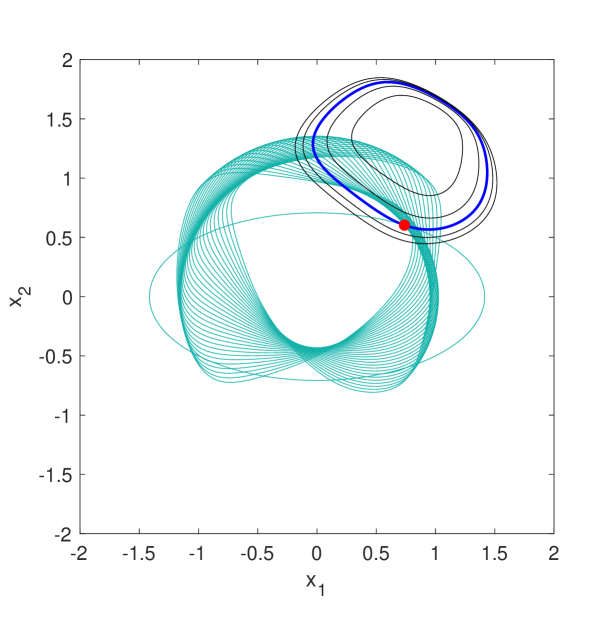
Figure 1. The feasible set $\mathbf{K}$ and contour curves of $f/g$ in Example 4.1

Next, we apply the ACA method to (31). It turns out that the first phase of ACA to find a consistent initial approximation of (31) with a reduced outer approximation of $\mathbf{Y}$ always failed. That is possibly because $\mathbf{Y}$ in (31) has no interior point and the upper level problem is not convex (c.f. [12, 50]). Then, we reformulate (31) to the following equivalent fractional semi-infinite programming problem involving trigonometric functions and a single parameter $t$

$$\min_{x\in{\mathbb{R}}^{2}}\ \frac{f(x)}{g(x)}\quad\text{s.t.}\ \psi(x)\leq 0,\ p(x,\sin t,\cos t)\leq 0,\ \ \forall t\in[0,\pi/2].$$ (32)

Then we solve (32) by the ACA method again. After a successful phase I, the first 10 iterations of phase II to compute an $\varepsilon$-stationary point of (32) run for about 22 minutes and produced a feasible point $(0.6530,0.6272)$. The 15th iteration of phase II produced a feasible point $(0.7374,0.6034)$ and the accumulated CPU time is about 40 minutes. The algorithm did not reach its default termination criterion within an hour. ∎

5. Special cases with exact or finitely convergent SDP relaxations

In this section, we study some cases of the FSIPP problem (1), for which we can derive SDP relaxation which is exact or has finite convergence and can extract at least one minimizer of (1). The reason for this concern is due to some applications of the FSIPP problem where exact optimal values and minimizers are required, see Section 5.2.

Recall the reformulations (10) and (11). Letting $\varepsilon=0$ in Theorem 3.1 implies that

Theorem 5.1.

Suppose that (A1-3) hold and the cones $\mathcal{C}[x]$ and $\mathcal{C}[y]$ satisfy the following conditions$:$ $\mathcal{C}[y]\subseteq\mathscr{P}(\mathbf{Y})$, $L_{f,g}(x,\mu^{\star},\eta^{\star})\in\mathcal{C}[x],$ there exists some $u^{\star}\in\mathbf{S}$ such that $-p(u^{\star},y)\in\mathcal{C}[y]$ and $h(u^{\star})\geq 0$ for any $h(x)\in\mathcal{C}[x]$.

1. We have $r^{\mbox{\tiny primal}}=r^{\mbox{\tiny dual}}=r^{\star}$.

2. If $\mathscr{L}^{\star}$ is a minimizer of (11) such that the restriction $\mathscr{L}^{\star}|_{{\mathbb{R}}[x]_{\mathbf{d}}}$ admits a representing nonnegative measure $\nu,$ then

   $$\frac{\mathscr{L}^{\star}(x)}{\mathscr{L}^{\star}(1)}=\frac{1}{\int d\nu}\left(\int x_{1}d\nu,\ldots,\int x_{m}d\nu\right)\in\mathbf{S}.$$

Next, we specify four cases of the FSIPP problem, for which we can choose suitable cones $\mathcal{C}[x]$ and $\mathcal{C}[y]$ with sum-of-squares structures and satisfy conditions in Theorem 5.1.

5.1. Four cases

Recall the s.o.s-convexity introduced in Section 2 and consider

1. (i) $n=1$ and $\mathbf{Y}=[-1,1]$; (ii) $f(x)$, $-g(x)$, $\psi_{i}(x),i=1,\ldots,s$, and $p(x,y)\in{\mathbb{R}}[x]$ for every $y\in\mathbf{Y}$ are all s.o.s-convex in $x$.

2. (i) $n>1$, $\mathbf{Y}=\{y\in{\mathbb{R}}^{n}\mid\phi(y)\geq 0\}$ where $\deg(\phi(y))=2$, $\phi(\bar{y})>0$ for some $\bar{y}\in{\mathbb{R}}^{n}$; (ii) $\deg_{y}(p(x,y))=2$; (iii) $f(x)$, $-g(x)$, $\psi_{i}(x),i=1,\ldots,s$, and $p(x,y)\in{\mathbb{R}}[x]$ for every $y\in\mathbf{Y}$ are all s.o.s-convex in $x$.

Let $d_{x}=\deg_{x}(p(x,y))$ and $d_{y}=\deg_{y}(p(x,y))$. For Case 1 and Case 2, we make the following choices of $\mathcal{C}[x]$ and $\mathcal{C}[y]$ in the reformulations (10) and (11):

1. Let

   $$\mathcal{C}[x]=\Sigma^{2}[x]\cap{\mathbb{R}}[x]_{2\mathbf{d}},$$ (33)

   and

   $$\mathcal{C}[y]=\left\{\theta_{0}+\theta_{1}(1-y_{1}^{2})\ \Big{|}\ \begin{aligned} &\theta_{0},\theta_{1}\in\Sigma^{2}[y_{1}],\deg(\theta_{0})\leq 2\lceil d_{y}/2\rceil,\\ &\deg(\theta_{1}(1-y_{1}^{2}))\leq 2\lceil d_{y}/2\rceil\end{aligned}\right\}.$$ (34)

2. Let $\mathcal{C}[x]$ be defined as in (33) and

   $$\mathcal{C}[y]=\{\theta+\lambda\phi\mid\lambda\geq 0,\ \theta\in\Sigma^{2}[y],\ \deg(\theta)\leq 2\}.$$ (35)

Recall Proposition 3.2 and Remark 3.1. In Case 1 and 2, we in fact choose $\mathcal{X}={\mathbb{R}}^{m}$ and $\Sigma^{2}[x]\cap{\mathbb{R}}[x]_{2\mathbf{d}}$ as the approximation of $\mathscr{P}(\mathcal{X})$. In each case, we can reduce (10) and (11) to a pair of primal and dual SDP problems.

Lemma 5.1.

Under (A1-2), if $f(x)$, $-g(x),$ $\psi_{i}(x),\ i=1,\ldots,s,$ and $p(x,y)\in{\mathbb{R}}[x]$ for every $y\in\mathbf{Y}$ are all s.o.s-convex in $x,$ then the Lagrangian $L_{f,g}(x,\mu,\eta)$ is s.o.s-convex for any $\mu\in\mathcal{M}(\mathbf{Y})$ and $\eta\in{\mathbb{R}}_{+}^{s}.$

Proof.

Obviously, we only need to prove that $\int_{\mathbf{Y}}p(x,y)d\mu(y)$ is s.o.s-convex under (A1-2). Note that there is a sequence of atomic measures $\{\mu_{k}\}\subseteq\mathcal{M}(\mathbf{Y})$ which is weakly convergent to $\mu$, i.e., $\lim_{k\rightarrow\infty}\int_{\mathbf{Y}}h(y)d\mu_{k}(y)=\int_{\mathbf{Y}}h(y)d\mu(y)$ holds for every bounded continuous real function $h(y)$ on $\mathbf{Y}$ (c.f. [5, Example 8.1.6 (i)]). It is obvious that $\int_{\mathbf{Y}}p(x,y)d\mu_{k}(y)\in{\mathbb{R}}[x]_{d_{x}}$ is s.o.s-convex for each $k$. Since the convex cone of s.o.s-convex polynomials in ${\mathbb{R}}[x]_{d_{x}}$ is closed (c.f. [2]), the conclusion follows.∎

Theorem 5.2.

In Cases $1$-$2:$ under (A2), the following holds.

1. $r^{\mbox{\tiny dual}}=r^{\star}$ and $\frac{\mathscr{L}^{\star}(x)}{\mathscr{L}^{\star}(1)}\in\mathbf{S}$ where $\mathscr{L}^{\star}$ be a minimizer of (11) which always exists.

2. If (A3) holds, then $r^{\mbox{\tiny primal}}=r^{\star}$ and it is attainable.

Proof.

In Case 1, by the representations of univariate polynomials nonnegative on an interval (c.f. [31, 41]), we have $-p(x,y)\in\mathcal{C}[y]$ for each $x\in\mathbf{K}$. In Case 2, by the $S$-lemma and Hilbert’s theorem, we also have $-p(x,y)\in\mathcal{C}[y]$ for each $x\in\mathbf{K}$. For any $u^{\star}\in\mathbf{S}$, the linear functional $\mathscr{L}^{\prime}\in({\mathbb{R}}[x])^{*}$ such that $\mathscr{L}^{\prime}(x^{\alpha})=\frac{(u^{\star})^{\alpha}}{g(u^{\star})}$ for each $\alpha\in\mathbb{N}^{m}$, is feasible to (11). Hence, $r^{\mbox{\tiny primal}}\leq r^{\mbox{\tiny dual}}\leq r^{\star}$ by the weak duality.

(i) Let $\mathscr{L}^{\star}$ be a minimizer of (11), then $\mathscr{L}^{\star}(1)>0$. In fact, $\mathscr{L}^{\star}(1)\geq 0$ since $\mathscr{L}^{\star}\in(\Sigma^{2}[x]\cap{\mathbb{R}}[x]_{2\mathbf{d}})^{*}$. If $\mathscr{L}^{\star}(1)=0$, then by the positive semidefiniteness of the associated moment matrix of $\mathscr{L}^{\star}$, we have $\mathscr{L}^{\star}(x^{\alpha})=0$ for all $\alpha\in\mathbb{N}^{m}_{\mathbf{d}}$, which contradicts the equality $\mathscr{L}^{\star}(g)=1$. As $\psi_{1}(x),\ldots,\psi_{s}(x)$, $p(x,y)\in{\mathbb{R}}[x]$ for every $y\in\mathbf{Y}$ are all s.o.s-convex in $x$, similar to the proof of Theorem 3.1 (ii), it is easy to see that $\frac{\mathscr{L}^{\star}(x)}{\mathscr{L}^{\star}(1)}\in\mathbf{K}$ due to Proposition 2.4. Since $f(x)$ and $-g(x)$ are also s.o.s-convex, under (A2), we have

$$r^{\star}\leq\frac{f\left(\frac{\mathscr{L}^{\star}(x)}{\mathscr{L}^{\star}(1)}\right)}{g\left(\frac{\mathscr{L}^{\star}(x)}{\mathscr{L}^{\star}(1)}\right)}\leq\frac{\frac{1}{\mathscr{L}^{\star}(1)}\mathscr{L}^{\star}(f)}{\frac{1}{\mathscr{L}^{\star}(1)}\mathscr{L}^{\star}(g)}=\mathscr{L}^{\star}(f)=r^{\mbox{\tiny dual}}\leq r^{\star}.$$

It means that $r^{\mbox{\tiny dual}}=r^{\star}$ and $\frac{\mathscr{L}^{\star}(x)}{\mathscr{L}^{\star}(1)}$ is minimizer of (1). Clearly, for any $u^{\star}\in\mathbf{S}$, the linear functional $\mathscr{L}^{\prime}\in({\mathbb{R}}[x]_{2\mathbf{d}})^{*}$ such that $\mathscr{L}^{\prime}(x^{\alpha})=\frac{(u^{\star})^{\alpha}}{g(u^{\star})}$ for each $\alpha\in\mathbb{N}^{m}_{2\mathbf{d}}$ is a minimizer of (11).

(ii) By Lemma 5.1, Proposition 3.1 and Lemma 2.1, $L_{f,g}(x,\mu^{\star},\eta^{\star})\in\mathcal{C}[x]$ in both cases. Thus, $r^{\mbox{\tiny primal}}=r^{\star}$ due to Theorem 5.1 (i) and is attainable at $(r^{\star},\mathscr{H},\eta^{\star})$ where $\mathscr{H}\in({\mathbb{R}}[y])^{*}$ satisfies that $\mathscr{H}(y^{\beta})=\int_{\mathbf{Y}}y^{\beta}d\mu^{\star}(y)$ for any $\beta\in\mathbb{N}^{n}$. ∎

Now we consider another two cases of the FSIPP problem (1):

1. (i) $n=1$ and $\mathbf{Y}=[-1,1]$; (ii) The Hessian $\nabla^{2}f(u^{\star})\succ 0$ at some $u^{\star}\in\mathbf{S}.$

2. (i) $n>1$, $\mathbf{Y}=\{y\in{\mathbb{R}}^{n}\mid\phi(y)\geq 0\}$ where $\deg(\phi(y))=2$, $\phi(\bar{y})>0$ for some $\bar{y}\in{\mathbb{R}}^{n}$; (ii) $\deg_{y}(p(x,y))=2$; (iii) The Hessian $\nabla^{2}f(u^{\star})\succ 0$ at some $u^{\star}\in\mathbf{S}$.

Let $R>0$ be a real number satisfying (18) and $q(x):=R^{2}-(x_{1}^{2}+\cdots+x_{m}^{2})$. For an integer $k\geq\lceil\mathbf{d}/2\rceil$, we make the following choices of $\mathcal{C}[x]$ and $\mathcal{C}[y]$ in the reformulations (10) and (11) in Case 3 and Case 4:

1. Replace $\mathcal{C}[x]$ by ${\mathcal{C}_{k}}[x]=\mathbf{qmodule}_{k}(\{q\})$ and let $\mathcal{C}[y]$ be defined as in (34).

2. Replace $\mathcal{C}[x]$ by ${\mathcal{C}_{k}}[x]=\mathbf{qmodule}_{k}(\{q\})$ and let $\mathcal{C}[y]$ be defined as in (35).

Recall Proposition 3.2 and Remark 3.1. In Case 3 and 4, we in fact choose $\mathcal{X}=\{x\in{\mathbb{R}}^{m}\mid q(x)\geq 0\}$ and quadratic modules generated by $\{q\}$ as the approximation of $\mathscr{P}(\mathcal{X})$. For a fixed $k$, in each case, denote the resulting problems of (10) and (11) by $(\ref{eq::f*r}k)$ and $(\ref{eq::f*rdual}k)$, respectively. Denote by $r^{\mbox{\tiny primal}}_{k}$ and $r^{\mbox{\tiny dual}}_{k}$ the optimal values of $(\ref{eq::f*r}k)$ and $(\ref{eq::f*rdual}k)$. We can reduce $(\ref{eq::f*r}k)$ and $(\ref{eq::f*rdual}k)$ to a pair of primal and dual SDP problems.

Theorem 5.3.

In Cases $3$-$4:$ under (A1-2), the following holds.

1. For each $k\geq\lceil\mathbf{d}/2\rceil,$ $r^{\mbox{\tiny primal}}_{k}\leq r^{\mbox{\tiny dual}}_{k}\leq r^{\star}$ and $r^{\mbox{\tiny dual}}_{k}$ is attainale.

2. For a minimizer $\mathscr{L}_{k}^{\star}$ of $(\ref{eq::f*rdual}k)$, if there exists an integer $k^{\prime}\in[\lceil\mathbf{d}/2\rceil,k]$ such that

   $$\mbox{rank}\ \mathbf{M}_{k^{\prime}-1}(\mathscr{L}_{k}^{\star})=\mbox{rank}\ \mathbf{M}_{k^{\prime}}(\mathscr{L}_{k}^{\star}),$$ (36)

   then, $r^{\mbox{\tiny dual}}_{k}=r^{\star}$ and $\frac{\mathscr{L}_{k}^{\star}(x)}{\mathscr{L}_{k}^{\star}(1)}$ is minimizer of (1);

3. If (A3) holds, then for $k$ large enough, $r_{k}^{\mbox{\tiny primal}}=r_{k}^{\mbox{\tiny dual}}=r^{\star}$ and every minimizer $\mathscr{L}_{k}^{\star}$ of $(\ref{eq::f*rdual}k)$ satisfies the rank condition (36) which certifies that $\frac{\mathscr{L}_{k}^{\star}(x)}{\mathscr{L}_{k}^{\star}(1)}$ is a minimizer of (1).

Proof.

(i) As proved in Theorem 5.2, we have $-p(u^{\star},y)\in\mathcal{C}[y]$ for every $u^{\star}\in\mathbf{S}\subset\mathbf{K}$ in both cases and hence $r^{\mbox{\tiny primal}}_{k}\leq r^{\mbox{\tiny dual}}_{k}\leq r^{\star}$. Due to the form of $q(x)$, the attainment of $r^{\mbox{\tiny dual}}_{k}$ follows from [26, Lemma 3] as proved in Theorem 4.2 (ii).

(ii) From the proof of Theorem 4.2 (iii), we can see that $\mathscr{L}_{k}^{\star}(1)>0$. By [9, Theorem 1.1], (36) implies that the restriction $\mathscr{L}_{k}^{\star}|_{{\mathbb{R}}[x]_{2k^{\prime}}}$ has an atomic representing measure supported on the set $\mathbf{K}^{\prime}:=\{x\in{\mathbb{R}}^{m}\mid q(x)\geq 0\}$. Then, the conclusion follows by Theorem 5.1 (ii).

(iii) Under (A1-3), consider the nonnegative Lagrangian $L_{f,g}(x,\mu^{\star},\eta^{\star})$. By Proposition 2.3, $L_{f,g}(x,\mu^{\star},\eta^{\star})$ is coercive and strictly convex on ${\mathbb{R}}^{m}$. Hence, by Proposition 3.1, $\mathbf{S}$ is a singleton set, say $\mathbf{S}=\{u^{\star}\}$, and $u^{\star}$ is the unique minimizer of $L_{f,g}(x,\mu^{\star},\eta^{\star})$ on ${\mathbb{R}}^{m}$. Clearly, $u^{\star}$ is an interior point of $\mathbf{K}^{\prime}$. Then, by Proposition 2.1, there exists $k^{\star}\in\mathbb{N}$ such that $L_{f,g}(x,\mu^{\star},\eta^{\star})\in\mathbf{qmodule}_{k^{\star}}(\{q\})$. Thus, in both Case 3 and Case 4, $L_{f,g}(x,\mu^{\star},\eta^{\star})\in{\mathcal{C}_{k}}[x]$ for every $k\geq k^{\star}$. Then, $r^{\mbox{\tiny primal}}_{k}=r^{\mbox{\tiny dual}}_{k}=r^{\star}$ for each $k\geq k^{\star}$ by Theorem 5.1 (i).

Consider the polynomial optimization problem

$$l^{\star}:=\min_{x\in{\mathbb{R}}^{m}}\ L_{f,g}(x,\mu^{\star},\eta^{\star})\quad\text{s.t.}\quad q(x)\geq 0.$$ (37)

Then, $l^{\star}=0$ and is attained at $u^{\star}$. The $k$-th Lasserre’s relaxation (see Section 2) for (37) is

$$l_{k}^{\mbox{\tiny dual}}:=\inf_{\mathscr{L}}\ \mathscr{L}(L_{f,g}(x,\mu^{\star},\eta^{\star}))\quad\text{s.t.}\ \ \mathscr{L}\in(\mathbf{qmodule}_{k}(\{q\}))^{*},\ \mathscr{L}(1)=1,$$ (38)

and its dual problem is

$$l_{k}^{\mbox{\tiny primal}}:=\sup_{\rho\in{\mathbb{R}}}\ \rho\quad\text{s.t.}\ \ L_{f,g}(x,\mu^{\star},\eta^{\star})-\rho\in\mathbf{qmodule}_{k}(\{q\}).$$ (39)

We have shown that $l_{k^{\star}}^{\mbox{\tiny primal}}\geq 0$. As the linear functional $\mathscr{L}^{\prime}\in({\mathbb{R}}[x]_{2k})^{*}$ with $\mathscr{L}^{\prime}(x^{\alpha})=(u^{\star})^{\alpha}$ for each $\alpha\in\mathbb{N}^{m}_{2k}$ is feasible to (38), along with the weak duality, we have $l_{k}^{\mbox{\tiny primal}}\leq l_{k}^{\mbox{\tiny dual}}\leq l^{\star}=0$, which means $l_{k^{\star}}^{\mbox{\tiny primal}}=l_{k^{\star}}^{\mbox{\tiny dual}}=0$. Hence, Lasserre’s hierarchy (38) and (39) have finite convergence at the order $k^{\star}$ without dual gap and the optimal value of (39) is attainable. Moreover, recall that $u^{\star}$ is the unique point in ${\mathbb{R}}^{m}$ such that $L_{f,g}(u^{\star},\mu^{\star},\eta^{\star})=0=l^{\star}$. Then by Proposition 2.2, the rank condition (36) holds for every minimizer of (38) for sufficiently large $k$. Let $\mathscr{L}_{k}^{\star}$ be a minimizer of $(\ref{eq::f*rdual}k)$ with $k\geq k^{\star}$. Now we show that $\frac{\mathscr{L}_{k}^{\star}}{\mathscr{L}_{k}^{\star}(1)}$ is a minimizer of (38). Clearly, $\frac{\mathscr{L}_{k}^{\star}}{\mathscr{L}_{k}^{\star}(1)}$ is feasible to (38). Because

$$0 =l^{\star}=l_{k}^{\mbox{\tiny dual}}\leq\frac{\mathscr{L}_{k}^{\star}(L_{f,g}(x,\mu^{\star},\eta^{\star}))}{\mathscr{L}_{k}^{\star}(1)}$$

$$=\frac{1}{\mathscr{L}_{k}^{\star}(1)}\left(\mathscr{L}_{k}^{\star}(f)-r^{\star}\mathscr{L}_{k}^{\star}(g)+\int_{\mathbf{Y}}\mathscr{L}_{k}^{\star}(p(x,y))d\mu^{\star}+\sum_{j=1}^{s}\eta_{j}\mathscr{L}_{k}^{\star}(\psi_{j})\right)$$

$$=\frac{1}{\mathscr{L}_{k}^{\star}(1)}\left(r^{\star}-r^{\star}+\int_{\mathbf{Y}}\mathscr{L}_{k}^{\star}(p(x,y))d\mu^{\star}+\sum_{j=1}^{s}\eta_{j}\mathscr{L}_{k}^{\star}(\psi_{j})\right)\leq 0,$$

$\frac{\mathscr{L}_{k}^{\star}}{\mathscr{L}_{k}^{\star}(1)}$ is indeed a minimizer of (38). Therefore, for $k$ sufficiently large, the rank condition (36) holds for $\frac{\mathscr{L}_{k}^{\star}}{\mathscr{L}_{k}^{\star}(1)}$ and hence for $\mathscr{L}_{k}^{\star}$. ∎

Example 5.1.

Now we consider four FSIPP problems corresponding to the four cases studied above.

Case 1: Consider the FSIPP problem

$$\left\{\begin{aligned} \min_{x\in{\mathbb{R}}^{2}}\ &\frac{(x_{1}+1)^{2}+(x_{2}+1)^{2}}{-x_{1}-x_{2}+1}\\ \text{s.t.}\ &p(x,y)=x_{1}^{2}+y^{2}x_{2}^{2}+2yx_{1}x_{2}+x_{1}+x_{2}\leq 0,\\ &\forall\ y\in[-1,1].\end{aligned}\right.$$ (40)

For any $y\in[-1,1]$, since $p(x,y)$ is of degree $2$ and convex in $x$, it is s.o.s-convex in $x$. Hence, the problem (40) is in Case 1. For any $x\in{\mathbb{R}}^{2}$ and $y\in[-1,1]$, it is clear that

$$p(x,y)\leq x_{1}^{2}+x_{2}^{2}+2|x_{1}x_{2}|+x_{1}+x_{2}.$$

Then we can see that the feasible set $\mathbf{K}$ can be defined only by two constraints

$$p(x,1)=(x_{1}+x_{2})(x_{1}+x_{2}+1)\leq 0\ \text{and}\ p(x,-1)=(x_{1}-x_{2})^{2}+x_{1}+x_{2}\leq 0.$$

That is, $\mathbf{K}$ is the area in ${\mathbb{R}}^{2}$ enclosed by the ellipse $p(x,-1)=0$ and the two lines $p(x,1)=0$. Then, it is not hard to check that the only global minimizer of (40) is $u^{\star}=(-0.5,-0.5)$ and the minimum is $0.25$. Obviously, (A2) holds for (40). Solving the single SDP problem (11) with the setting (33) and (34), we get $\frac{\mathscr{L}^{\star}(x)}{\mathscr{L}^{\star}(1)}=(-0.5000,-0.5000)$ where $\mathscr{L}^{\star}$ is the minimizer of (11). The CPU time is $0.80$ seconds. Then we solve (40) with ACA method. The algorithm terminated successfully and returned the solution $(-0.5000,-0.5000)$. The over CPU time is $4.25$ seconds.

Case 2: Consider the FSIPP problem

$$\left\{\begin{aligned} \min_{x\in{\mathbb{R}}^{2}}\ &\frac{(x_{1}-1)^{2}+(x_{2}-1)^{2}}{x_{1}+x_{2}}\\ \text{s.t.}\ &\psi(x)=(x_{1}+x_{2}-1)(x_{1}+x_{2}-0.5)\leq 0,\\ &p(x,y)=(y_{1}^{2}+y_{2}^{2})x_{1}^{2}+(1/2-y_{1}y_{2})x_{2}^{2}-1\leq 0,\ \forall\ y\in\mathbf{Y},\\ &\mathbf{Y}=\{y\in{\mathbb{R}}^{2}\mid y_{1}^{2}+y_{2}^{2}\leq 1\}.\end{aligned}\right.$$ (41)

It is easy to see that (41) is in Case 2. For any $y\in\mathbf{Y}$, it holds that

$$p(x,y)\leq x_{1}^{2}+x_{2}^{2}-1=p(x,y^{(0)}),\quad y^{(0)}=\left(-\frac{\sqrt{2}}{2},\frac{\sqrt{2}}{2}\right).$$

Hence, $\mathbf{K}$ is the part of the unit disc around the origin between the two lines defined by $\psi(x)=0$ and the only global minimizer is $u^{\star}=(0.5,0.5)$. Obviously, (A2) holds for (41). Solving the single SDP problem (11) with the setting (33) and (35), we get $\frac{\mathscr{L}^{\star}(x)}{\mathscr{L}^{\star}(1)}=(0.4999,0.5000)$ where $\mathscr{L}^{\star}$ is the minimizer of (11). The CPU time is $1.20$ seconds. Then we solve (41) with ACA method. The algorithm terminated successfully and returned the solution $(0.5000,0.5000)$. The overall CPU time is $52.75$ seconds.

Case 3: Recall the convex but not s.o.s-convex polynomial $h_{2}(x)$ in (30). Consider the FSIPP problem

$$\left\{\begin{aligned} \min_{x\in{\mathbb{R}}^{2}}\ &\frac{(x_{1}-1)^{2}+(x_{2}-1)^{2}-2}{-x_{1}-x_{2}+4}\\ \text{s.t.}\ &\psi(x)=x_{1}^{2}+x_{2}^{2}-4\leq 0,\\ &p(x,y)=\frac{h_{2}(x_{1},x_{2})}{1000}-yx_{1}-y^{2}x_{2}-1\leq 0,\ \forall\ y\in[-1,1].\end{aligned}\right.$$ (42)

Clearly, this problem is in Cases $3$ and satisfies (A1-2). We solve the SDP relaxation $(\ref{eq::f*rdual}k)$ with the setting ${\mathcal{C}_{k}}[x]$ and $\mathcal{C}[y]$ aforementioned. We set the first order $k=4$ and check if the rank condition (36) holds. If not, check the next order. We have $\mbox{rank}\mathbf{M}_{3}(\mathscr{L}_{4}^{\star})=\mbox{rank}\mathbf{M}_{4}(\mathscr{L}_{4}^{\star})=1$ (within a tolerance $<10^{-8}$) for a minimizer $\mathscr{L}_{4}^{\star}$ of of $r^{\mbox{\tiny dual}}_{4}$, i.e., the rank condition (36) holds for $k^{\prime}=4$. By Theorem 5.3 (ii), the point $u^{\star}:=\frac{\mathscr{L}_{4}^{\star}(x)}{\mathscr{L}_{4}^{\star}(1)}=(0.9044,0.8460)$ is a minimizer and $r^{\mbox{\tiny dual}}_{4}=-0.8745$ is the minimum of (42). The CPU time is about $16.50$ seconds. To show the accuracy of the solution , we draw some contour curves of $f/g$, including the one where $f/g$ is the constant value $f(u^{\star})/g(u^{\star})=-0.8745$ (the blue curve), and mark the point $u^{\star}$ by a red dot in Figure 2 (left). Then we solve (42) with the ACA method. The algorithm terminated successfully and returned the solution $(0.9040,0.8463)$. The overall CPU time is $21.57$ seconds.

Case 4: Consider the FSIPP problem

$$\left\{\begin{aligned} \min_{x\in{\mathbb{R}}^{2}}\ &\frac{(x_{1}-2)^{2}+(x_{2}-2)^{2}-1}{-x_{1}^{2}-x_{2}^{2}+4}\\ \text{s.t.}\ &\psi(x)=x_{1}^{2}+x_{2}^{2}-1\leq 0,\\ &p(x,y)=\frac{h_{2}(x_{1},x_{2})}{1000}+y_{1}y_{2}(x_{1}+x_{2})-1\leq 0,\ \forall\ y\in\mathbf{Y},\\ &\mathbf{Y}=\{y\in{\mathbb{R}}^{2}\mid y_{1}^{2}+y_{2}^{2}\leq 1\}.\end{aligned}\right.$$ (43)

Clearly, this problem is in Cases $4$ and satisfies (A1-2). We solve the SDP relaxation $(\ref{eq::f*rdual}k)$ with the setting ${\mathcal{C}_{k}}[x]$ and $\mathcal{C}[y]$ aforementioned. For the first order $k=4$, we have $\mbox{rank}\mathbf{M}_{3}(\mathscr{L}_{4}^{\star})=\mbox{rank}\mathbf{M}_{4}(\mathscr{L}_{4}^{\star})=1$ (within a tolerance $<10^{-8}$) for a minimizer $\mathscr{L}_{4}^{\star}$ of of $r^{\mbox{\tiny dual}}_{4}$. By Theorem 5.3 (ii), the point $u^{\star}:=\frac{\mathscr{L}_{4}^{\star}(x)}{\mathscr{L}_{4}^{\star}(1)}=(0.7211,0.6912)$ is a minimizer of (43). The CPU time is about $14.60$ seconds. See Figure 2 (right) for the accuracy of the solution. Then we solve (43) with the ACA method. The algorithm terminated successfully and returned the solution $(0.7039,0.6823)$. The overall CPU time is $768.02$ seconds.

For the above four FSIPP problems, we remark that the optimality of the solution obtained by our SDP method can be guaranteed by Theorem 5.2 (i) and Theorem 5.3 (ii), while the solution concept of the ACA method is that of stationary points and all iterates are feasible points for the original SIP. ∎

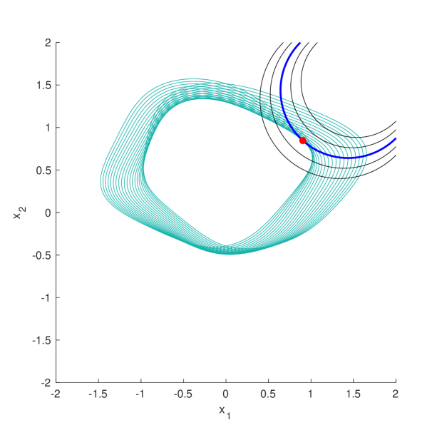
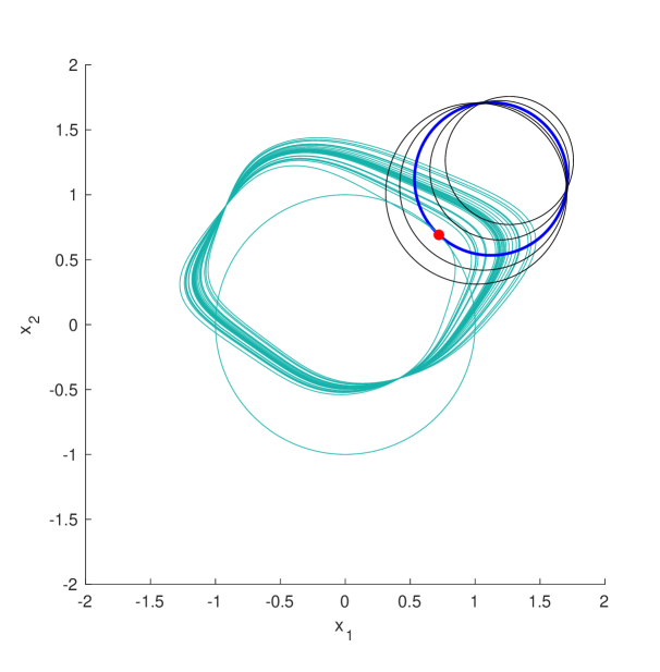
Figure 2. The feasible set $\mathbf{K}$ and contour curves of $f/g$ in Example 5.1 Case 3 (left) and Case 4 (right).

5.2. Application to Multi-objective FSIPP

In this part, we apply the above approach for the special four cases of FSIPP problems to the following multi-objective fractional semi-infinite polynomial programming (MFSIPP) problem

$$\left\{\begin{aligned} {\rm Min}_{{\mathbb{R}}^{t}_{+}}&\ \left(\frac{f_{1}(x)}{g_{1}(x)},\ldots,\frac{f_{t}(x)}{g_{t}(x)}\right)\\ \text{s.t.}&\ p(x,y)\leq 0,\ \ \forall y\in\mathbf{Y}\subset{\mathbb{R}}^{n},\end{aligned}\right.$$ (44)

where $f_{i}(x),g_{i}(x)\in{\mathbb{R}}[x],$ $i=1,\ldots,t,$ $p(x,y)\in{\mathbb{R}}[x,y]$. Note that “${\rm Min_{{\mathbb{R}}^{t}_{+}}}$” in the above problem (44) is understood in the vectorial sense, where a partial ordering is induced in the image space ${\mathbb{R}}^{t},$ by the non-negative cone ${\mathbb{R}}^{t}_{+}.$ Let $a,b\in{\mathbb{R}}^{t},$ the partial ordering says that $a\geq b$ (or $a-b\in{\mathbb{R}}^{t}_{+}$), which can equivalently be written as $a_{i}\geq b_{i},$ for all $i=1,\ldots,t,$ where $a_{i}$ and $b_{i}$ stands for the $i$th component of the vectors $a$ and $b,$ respectively. Denote by $\mathbf{F}$ the feasible set of (44). We make the following assumptions on the MFSIPP problem (44):

(A5): $\mathbf{Y}$ is compact; $f_{i}(x)$, $-g_{i}(x)$, $i=1,\ldots,t,$ and $p(x,y)\in{\mathbb{R}}[x]$ for every $y\in\mathbf{Y}$ are all convex in $x$;
(A6): For each $i=1,\ldots,t$, either $f_{i}(x)\geq 0$ and $g_{i}(x)>0$ for all $x\in\mathbf{F}$; or $g_{i}(x)$ is affine and $g_{i}(x)>0$ for all $x\in\mathbf{F}$.

Definition 5.1.

A point $u^{\star}\in\mathbf{F}$ is said to be an efficient solution to (44) if

$$\left(\frac{f_{1}(x)}{g_{1}(x)},\ldots,\frac{f_{t}(x)}{g_{t}(x)}\right)-\left(\frac{f_{1}(u^{\star})}{g_{1}(u^{\star})},\ldots,\frac{f_{t}(u^{\star})}{g_{t}(u^{\star})}\right)\not\in-{\mathbb{R}}^{t}_{+}\backslash\{0\},\quad\forall x\in\mathbf{F}.$$ (45)

Efficient solutions to (44) are also known as Pareto-optimal solutions. The aim of this part is to find efficient solutions to (44). As far as we know, very few algorithmic developments are available for such a case in the literature because of the difficulty of checking feasibility of a given point.

The $\epsilon$-constraint method [17, 6] may be the best known technique to solve a nonconvex multi-objective optimization problem. The basic idea for this method is to minimize one of the original objectives while the others are transformed to constraints by setting an upper bound to each of them. Based on the criteria for the $\epsilon$-constraint method given in [11], an algorithm to obtain an efficient solution to (44) follows.

Algorithm 5.1.

(Compute an efficient solution $u^{\star}$ to the MFSIPP problem (44).)

1. Set $i=1$ and choose an initial point $u^{(i-1)}\in\mathbf{F}$.

2. Solve the single objective FSIPP problem

   $$r_{i}:=\min_{x\in\mathbf{F}}\ \frac{f_{i}(x)}{g_{i}(x)}\quad\text{s.t.}\ \ g_{j}(u^{(i-1)})f_{j}(x)-f_{j}(u^{(i-1)})g_{j}(x)\leq 0,\ \ j\neq i. \mathrm{P}_{i}$$ ()

   and extract a minimizer $u^{(i)}$ of ($\mathrm{P}_{i}$).

3. If either $u^{(i)}$ can be verified to be the unique minimizer of ($\mathrm{P}_{i}$) or $i=t$, return $u^{\star}=u^{(i)}$; otherwise, let $i=i+1$ and go to Step 2.

Theorem 5.4.

The output $u^{\star}$ in Algorithm 5.1 is indeed an efficient solution to (1).

Proof.

We refer to [11, Propositions 4.4 and 4.5]; see also [32, Theorem 3.4]. ∎

Remark 5.1.

• Clearly, ($\mathrm{P}_{i}$) is an FSIPP problem of the form (1). It is easy to see that for each $i=2,\ldots,t$, the constraints

  $$g_{j}(u^{(i-1)})f_{j}(x)-f_{j}(u^{(i-1)})g_{j}(x)\leq 0,\ j=1,\ldots,i-1,$$

  are all active in ($\mathrm{P}_{i}$). Therefore, the Slater condition fails for ($\mathrm{P}_{i}$) with $i=2,\ldots,t.$

• According to Algorithm 5.1, the problem of finding an efficient solution of the MFSIPP problem (44) reduces to solving every scalarized problem ($\mathrm{P}_{i}$) and extracting a (common) minimizer, which is the key for the success of Algorithm 5.1. Generally, approximate solutions to ($\mathrm{P}_{i}$) can be obtained by some numerical methods for semi-infinite programming problems. However, note that the errors introduced by any approximate solutions can accumulate in the process of the $\epsilon$-constraint method. This can potentially make the output solution unreliable.∎

We have studied four cases of the FSIPP problem, for which at least one minimizer can be extracted by the proposed SDP approach. Now we apply this approach to the four corresponding cases of MFSIPP problem:

Case I (resp., II):  ($\mathrm{P}_{i}$) is in Case 1 (resp., 2) for each $i=1,\ldots,t$;

Case III (resp., IV):  ($\mathrm{P}_{i^{\prime}}$) is in Case 3 (resp., 4) for some $i^{\prime}\in\{1,\ldots,t\}$.

For Case I and II, if the assumptions in Theorem 5.2 hold for each ($\mathrm{P}_{i}$), then an efficient solution to the MFSIPP problem (44) can obtained by solving $t$ SDP problems.

For Case III and IV, we only need solve ($\mathrm{P}_{i^{\prime}}$) to get an efficient solution to (44). In fact, we have the following result.

Proposition 5.1.

In Cases III-IV$:$ under (A5-6), the scalarized problem $(\mathrm{P}_{i^{\prime}})$ has a unique minimizer $u^{(i^{\prime})}$ which is an efficient solution to the MFSIPP problem (44).

Proof.

By assumption, $f_{i^{\prime}}(x)-r_{i^{\prime}}g_{i^{\prime}}(x)$ is convex and its minimum on the feasible set of ($\mathrm{P}_{i^{\prime}}$) is $0$ attained at any optimal solution of ($\mathrm{P}_{i^{\prime}}$). By Proposition 2.3, $f_{i^{\prime}}(x)-r_{i^{\prime}}g_{i^{\prime}}(x)$ is coercive and strictly convex on ${\mathbb{R}}^{m}$. Then, $f_{i^{\prime}}(x)-r_{i^{\prime}}g_{i^{\prime}}(x)$ has a unique minimizer on the feasible set of ($\mathrm{P}_{i^{\prime}}$). Consequently, ($\mathrm{P}_{i^{\prime}}$) has a unique minimizer $u^{(i^{\prime})}$. By Theorem 5.4, $u^{(i^{\prime})}$ is an efficient solution to (44). ∎

As a result, in Case III and Case IV, if the assumptions in Theorem 5.3 hold for ($\mathrm{P}_{i^{\prime}}$), an efficient solution to the MFSIPP problem (44) can be obtained by solving finitely many SDP problems.

Example 5.2.

To show the efficiency of the SDP method for the four cases of the MFSIPP problem discussed above, now we present an example for each case. In each of the following examples, $m=2$ and $t=2$. We pick some points $y$ on a uniform discrete grid inside $\mathbf{Y}$ and draw the corresponding curves $p(x,y)=0$. Hence, the feasible set $\mathbf{F}$ is illustrated by the area enclosed by these curves. The initial point $u^{(0)}$ and the output $u^{\star}$ of Algorithm 5.1 are marked in $\mathbf{F}$ by ‘$\ast$’ in blue and red, respectively. To show the accuracy of the output, we first illustrate the image of $\mathbf{F}$ under the map $\left(\frac{f_{1}}{g_{1}},\frac{f_{2}}{g_{2}}\right)$. To this end, we choose a square containing $\mathbf{F}$. For each point $u$ on a uniform discrete grid inside the square, we check if $u\in\mathbf{F}$ (as we will see it is easy for our examples). If so, we plot the point $\left(\frac{f_{1}(u)}{g_{1}(u)},\frac{f_{2}(u)}{g_{2}(u)}\right)$ in the image plane. The points $\left(\frac{f_{1}(u^{(0)})}{g_{1}(u^{(0)})},\frac{f_{2}(u^{(0)})}{g_{2}(u^{(0)})}\right)$ and $\left(\frac{f_{1}(u^{\star})}{g_{1}(u^{\star})},\frac{f_{2}(u^{\star})}{g_{2}(u^{\star})}\right)$ are then marked in the image by ‘$\ast$’ in blue and red, respectively. We will see from the figures that the output of Algorithm 5.1 in each example is indeed as we expect.

Case I: Consider the ellipse

$$\mathbf{F}=\{(x_{1},x_{2})\in{\mathbb{R}}^{2}\mid 2x_{1}^{2}+x_{2}^{2}+2x_{1}x_{2}+2x_{1}\leq 0\},$$

which can be represented by

$$\{(x_{1},x_{2})\in{\mathbb{R}}^{2}\mid p(x_{1},x_{2},y_{1})\leq 0,\ \forall y_{1}\in\mathbf{Y}\},$$

where

$$p(x_{1},x_{2},y_{1})=(y_{1}^{4}+2y_{1}^{3}-3y_{1}^{2}-2y_{1}+1)x_{1}+2y_{1}(y_{1}^{2}-1)x_{2}-2y_{1}^{2},$$

and $\mathbf{Y}=[-1,1]$ $($See [13]$)$. The feasible set $\mathbf{F}$ is illustrated in Figure 3 (left).

Consider the problem

$${\rm Min}_{{\mathbb{R}}^{2}_{+}}\left\{\left(\frac{f_{1}}{g_{1}},\frac{f_{2}}{g_{2}}\right):=\left(\frac{x_{1}^{2}+x_{2}}{x_{2}+1},\ x_{1}^{2}-x_{2}+x_{1}\right)\Big{|}\ x\in\mathbf{F}\right\}.$$

Clearly, this problem is in Case I. By checking if a given point is in the ellipse $\mathbf{F}$, it is easy to depict the image of $\mathbf{F}$ in the way aforementioned, which is shown in Figure 3 (right). Let the initial point be $u^{(0)}=(-1,1)$ in Algorithm 5.1. The output is $u^{\star}=u^{(2)}=(-0.2138,0.8319)$. These points and their images are marked in Figure 3.

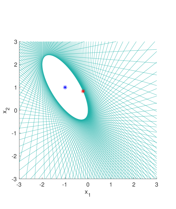
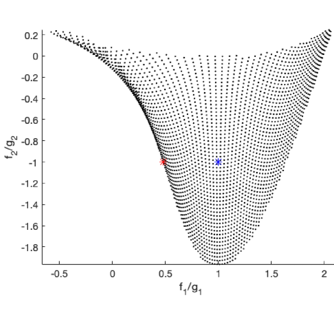
Figure 3. The feasible set $\mathbf{F}$ (left) and its image (right) in the example of Case I.

Case II: Consider the set

$$\mathbf{F}=\{(x_{1},x_{2})\in{\mathbb{R}}^{2}\mid p(x_{1},x_{2},y_{1},y_{2})\leq 0,\quad\forall y\in\mathbf{Y}\}$$

where $p(x_{1},x_{2},y_{1},y_{2})=-1+x_{1}^{2}+x_{2}^{2}+(y_{1}-y_{2})^{2}x_{1}x_{2}$ and

$$\mathbf{Y}=\{(y_{1},y_{2})\in{\mathbb{R}}^{2}\mid 1-y_{1}^{2}-y_{2}^{2}\geq 0\}.$$

The set $\mathbf{F}$ is illustrated in Figure 4 (left). The Hessian matrix of $p$ with respect to $x_{1}$ and $x_{2}$ is

$$H=\left[\begin{array}[]{cc}2&(y_{1}-y_{2})^{2}\\ (y_{1}-y_{2})^{2}&2\end{array}\right]\qquad\text{with}\quad\det(H)=4-(y_{1}-y_{2})^{4}.$$

It is easy to see that $p(x_{1},x_{2},y_{1},y_{2})$ is s.o.s-convex in $(x_{1},x_{2})$ for every $y\in\mathbf{Y}$.

Consider the problem

$${\rm Min}_{{\mathbb{R}}^{2}_{+}}\left\{\left(\frac{f_{1}}{g_{1}},\frac{f_{2}}{g_{2}}\right):=\left(\frac{x_{2}^{2}-x_{1}+1}{-x_{1}^{2}+2},\ x_{1}^{2}+x_{2}+x_{1}\right)\Big{|}\ x\in\mathbf{F}\right\}.$$

Clearly, this problem is in Case II. To depict the image of $\mathbf{F}$ in the aforementioned way, we remark that $\mathbf{F}$ is in fact the area enclosed by the lines $x_{1}+x_{2}=\pm 1$ and the unit circle. Hence, it is easy to check whether a given point is in $\mathbf{F}$. The image of $\mathbf{F}$ is shown in Figure 4 (right). Let the initial point be $u^{(0)}=(0,1)$ in Algorithm 5.1. The output is $u^{\star}=u^{(2)}=(0.6822,-0.1476)$. These points and their images are marked in Figure 4.

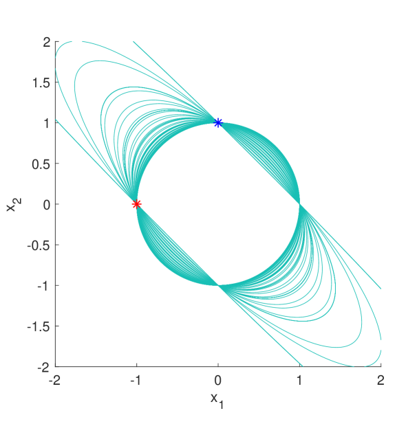
Figure 4. The feasible set $\mathbf{F}$ (left) and its image (right) in the example of Case II.

Case III: Consider the polynomial $h_{1}(x_{1},x_{2},x_{3})$ in (30) and let

$$\mathbf{F}=\{(x_{1},x_{2})\in{\mathbb{R}}^{2}\mid p(x_{1},x_{2},y_{1})\leq 0,\quad\forall y_{1}\in\mathbf{Y}\},$$

where $p(x_{1},x_{2},y_{1})=-1+h_{1}(x_{1},x_{2},1)/100-y_{1}x_{1}-y_{1}^{2}x_{2}$ and $\mathbf{Y}=[-1,1]$. Clearly, $p(x,y_{1})$ is convex but not s.o.s-convex for every $y_{1}\in\mathbf{Y}$. We illustrate $\mathbf{F}$ in Figure 5 (left).

Consider the problem

$${\rm Min}_{{\mathbb{R}}^{2}_{+}}\left\{\left(\frac{f_{1}}{g_{1}},\frac{f_{2}}{g_{2}}\right):=\left(\frac{x_{1}^{2}+x_{2}^{2}+1}{-x_{1}^{2}-x_{2}+3},\ x_{1}^{2}+x_{2}^{2}-x_{1}+1\right)\Big{|}\ x\in\mathbf{F}\right\}.$$ (46)

For a given point $u\in{\mathbb{R}}^{2}$, as $p(u_{1},u_{2},y_{1})$ is a univariate quadratic function, it is easy to check whether $-p(u_{1},u_{2},y_{1})$ is nonnegative on $[-1,1]$ (i.e., whether $u\in\mathbf{F}$). Hence, The image of $\mathbf{F}$ can be easily depicted in Figure 5 (right). Clearly, ($\mathrm{P}_{1}$) is in Case 3. Hence, we only need to solve ($\mathrm{P}_{1}$) to get an efficient solution by Proposition 5.1 and Theorem 5.4. We let the initial point be $u^{(0)}=(-0.6,0.5)$ in Algorithm 5.1 and solve ($\mathrm{P}_{1}$) by the SDP relaxations for Case 3. We set the first order $k=4$ and check if the rank condition (36) holds. If not, check the next order. We have $\mbox{rank}\mathbf{M}_{3}(\mathscr{L}_{4}^{\star})=\mbox{rank}\mathbf{M}_{4}(\mathscr{L}_{4}^{\star})=1$ (within a tolerance $<10^{-8}$) for a minimizer $\mathscr{L}_{4}^{\star}$ of of $r^{\mbox{\tiny dual}}_{4}$, i.e., the rank condition (36) holds for $k^{\prime}=4$. By Theorem 5.3 (ii), the point $u^{\star}:=\frac{\mathscr{L}_{4}^{\star}(x)}{\mathscr{L}_{4}^{\star}(1)}=(0.000,-0.1623)$ is an efficient solution to (46). These points $u^{(0)},u^{\star}$ and their images are marked in Figure 5.

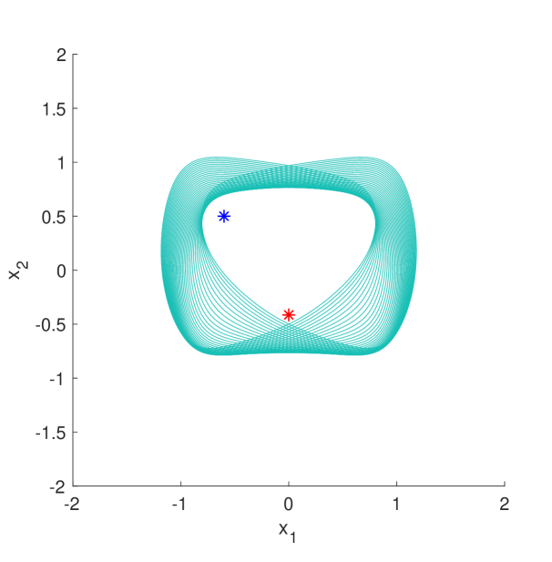
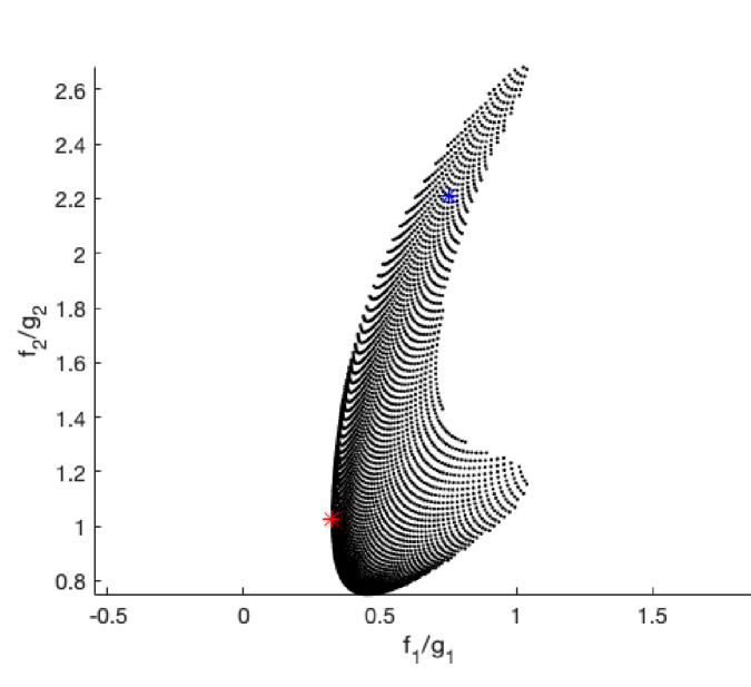
Figure 5. The feasible set $\mathbf{F}$ (left) and its image (right) in the example of Case III.

Case IV: Let $h_{1}(x_{1},x_{2},x_{3})$ be the polynomial in (30) and

$$\mathbf{F}=\{(x_{1},x_{2})\in{\mathbb{R}}^{2}\mid p(x_{1},x_{2},y_{1},y_{2})\leq 0,\quad\forall y\in\mathbf{Y}\},$$

where $p(x_{1},x_{2},y_{1},y_{2})=(h_{1}(x_{1},x_{2},1)/100-1)-y_{1}y_{2}(x_{1}+x_{2})$ and

$$\mathbf{Y}=\{(y_{1},y_{2})\in{\mathbb{R}}^{2}\mid 1-y_{1}^{2}-y_{2}^{2}\geq 0\}.$$

Clearly, $p(x,y)$ is convex but not s.o.s-convex for every $y\in\mathbf{Y}$. We illustrate $\mathbf{F}$ in Figure 6 (left).

Consider the problem

$${\rm Min}_{{\mathbb{R}}^{2}_{+}}\left\{\left(\frac{f_{1}}{g_{1}},\frac{f_{2}}{g_{2}}\right):=\left(\frac{x_{1}^{2}+x_{2}^{2}+1}{-x_{2}^{2}+x_{1}+4},\ \frac{x_{1}^{2}+x_{2}}{x_{1}+x_{2}+2}\right)\Big{|}\ x\in\mathbf{F}\right\}.$$ (47)

To depict the image of $\mathbf{F}$ in the aforementioned way, we remark that $\mathbf{F}$ is in fact the area enclosed by the two curves $p\left(x_{1},x_{2},\pm\frac{\sqrt{2}}{2},\pm\frac{\sqrt{2}}{2}\right)=0$. Hence, it is easy to check whether a given point is in $\mathbf{F}$. Then the image of $\mathbf{F}$ can be easily depicted in Figure 6 (right). Clearly, ($\mathrm{P}_{1}$) is in Case 4. Again, we only need to solve ($\mathrm{P}_{1}$). We let the initial point be $u^{(0)}=(-0.5,0.5)$ in Algorithm 5.1 and solve ($\mathrm{P}_{1}$) by the SDP relaxations for Case 4. We check if the rank condition (36) holds for the order initialized from $4$. Similarly to Case III, when $k=4$ and $k^{\prime}=4$, the rank condition (36) holds for a minimizer $\mathscr{L}_{4}^{\star}$ of $r^{\mbox{\tiny dual}}_{4}$. By Theorem 5.3 (ii), the point $u^{\star}:=\frac{\mathscr{L}_{4}^{\star}(x)}{\mathscr{L}_{4}^{\star}(1)}=(0.1231,0.000)$ is an efficient solution to (47). These points $u^{(0)},u^{\star}$ and their images are marked in Figure 6. ∎

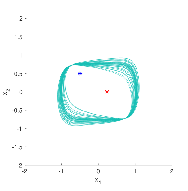
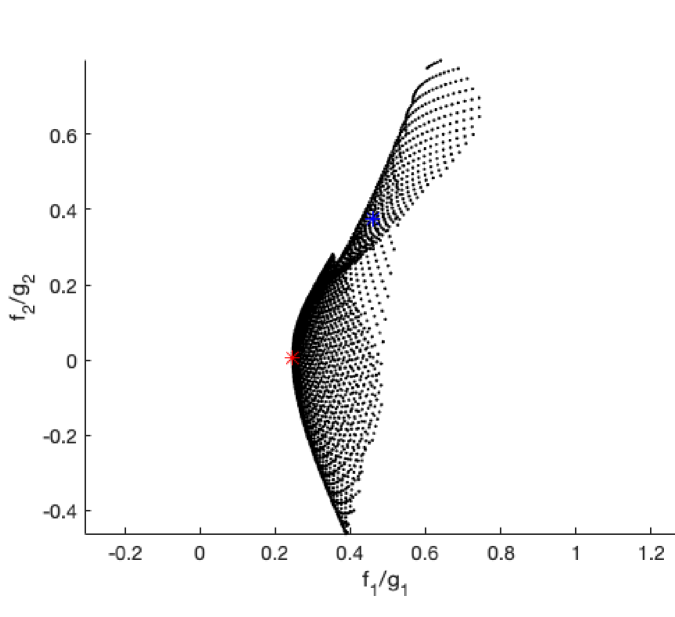
Figure 6. The feasible set $\mathbf{F}$ (left) and its image (right) in the example of Case IV.

6. Conclusions

We focus on solving a class of FSIPP problems with some convexity/concavity assumption on the function data. We reformulate the problem to a conic optimization problem and provide a characteristic cone constraint qualification for convex SIP problems to bring sum-of-squares structures in the reformulation. In this framework, we first present a hierarchy of SDP relaxations with asymptotic convergence for the FSIPP problem whose index set is defined by finitely many polynomial inequalities. Next, we study four cases of the FSIPP problems for which the SDP relaxation is exact or has finite convergence and at least one minimizer can be extracted. This approach is then applied to the four corresponding multi-objective cases to find efficient solutions.

Appendix A

Consider the general convex semi-infinite programming problem

$$\left\{\begin{aligned} r^{\star}:=\inf_{x\in{\mathbb{R}}^{m}}&\ h(x)\\ \text{s.t.}&\ \psi_{1}(x)\leq 0,\ldots,\psi_{s}(x)\leq 0,\\ &\ p(x,y)\leq 0,\quad\forall\ y\in\mathbf{Y}\subset{\mathbb{R}}^{n},\end{aligned}\right.$$ (48)

where $h(\cdot)$, $\psi_{1}(\cdot),\ldots,\psi_{s}(\cdot)$, $p(\cdot,y):{\mathbb{R}}^{m}\rightarrow{\mathbb{R}}$ for any $y\in\mathbf{Y}$, are continuous and convex functions (not necessarily polynomials), $p(x,y):{\mathbb{R}}^{m}\times{\mathbb{R}}^{n}\rightarrow{\mathbb{R}}$ is a lower semicontinuous function such that $p(x,\cdot):{\mathbb{R}}^{n}\rightarrow{\mathbb{R}}$ is continuous for all $x\in{\mathbb{R}}^{m}$, the index set $\mathbf{Y}$ is an arbitrary compact subset in ${\mathbb{R}}^{n}$. We denote by $\mathbf{K}$ the feasible region of (48) and assume that $\mathbf{K}\neq\emptyset$. Inspired by Jeyakumar and Li [23], we next provide a constraint qualification weaker than the Slater condition for (48) to guarantee the strong duality and the attachment of the solution in the dual problem.

Denote by $\mathcal{M}(\mathbf{Y})$ the set of nonnegative measures supported on $\mathbf{Y}$. We first show that for all $\mu\in\mathcal{M}(\mathbf{Y}),$

$$\Phi_{\mu}:x\mapsto\int_{\mathbf{Y}}p(x,y)d\mu(y)$$

is a continuous and convex function. Indeed, it is clear that this function always takes finite value due to the continuity assumption of $p(x,\cdot)$ for all $x\in{\mathbb{R}}^{m}$. Now, by Fatou’s lemma, for any $x^{(k)}\rightarrow x,$

$$\liminf_{k\rightarrow\infty}\int_{\mathbf{Y}}p(x^{(k)},y)d\mu(y)\geq\int_{\mathbf{Y}}p(x,y)d\mu(y).$$

This shows that $\Phi_{\mu}$ is a lower semicontinuous function. Also, as $p(\cdot,y)$ is convex and $\mu\in\mathcal{M}(\mathbf{Y})$, it is easy to see that $\Phi_{\mu}$ is also convex for all $\mu\in\mathcal{M}(\mathbf{Y})$. Thus, $\Phi_{\mu}$ is a proper lower semicontinuous convex function which always takes finite value, and so, is continuous.

The Lagrangian dual of (48) reads

$$\max_{\mu\in\mathcal{M}(\mathbf{Y}),\eta\in{\mathbb{R}}_{+}^{s}}\inf_{x\in{\mathbb{R}}^{m}}\left\{h(x)+\int_{\mathbf{Y}}p(x,y)d\mu(y)+\sum_{j=1}^{s}\eta_{j}\psi_{j}(x)\right\}.$$ (49)

Recall the notation in (16),

$$\mathcal{C}_{1}=\bigcup_{\mu\in\mathcal{M}(\mathbf{Y})}\text{epi}\left(\int_{\mathbf{Y}}p(\cdot,y)d\mu(y)\right)^{*}\ \text{and}\ \mathcal{C}_{2}=\bigcup_{\eta\in{\mathbb{R}}_{+}^{s}}\text{epi}\left(\sum_{j=1}^{s}\eta_{j}\psi_{j}\right)^{*}.$$

We say that the semi-infinite characteristic cone constraint qualification (SCCCQ) holds for $\mathbf{K}$ if $\mathcal{C}_{1}+\mathcal{C}_{2}$ is closed.

Proposition A.1.

The set $\mathcal{C}_{1}+\mathcal{C}_{2}$ is a convex cone.

Proof.

As $\mathcal{C}_{2}$ is a convex cone due to [10, Theorem 2.123], we only need to prove that $\mathcal{C}_{1}$ is a convex cone.

We first prove that $\mathcal{C}_{1}$ is a cone. It is clear that $(0,0)\in\mathcal{C}_{1}$. Let $\lambda>0$ and $(\xi,\alpha)\in\mathcal{C}_{1}$ Then, there exists $\mu^{\prime}\in\mathcal{M}(\mathbf{Y})$ such that $(\xi,\alpha)\in\text{epi}\left(\int_{\mathbf{Y}}p(\cdot,y)d\mu^{\prime}(y)\right)^{*}$. Let $\tilde{\mu}=\lambda\mu^{\prime}\in\mathcal{M}(\mathbf{Y})$. As $\Phi_{\mu^{\prime}}$ is continuous and convex, by [10, Theorem 2.123 (iv)],

$$\lambda(\xi,\alpha)\in\lambda\text{epi}\left(\int_{\mathbf{Y}}p(\cdot,y)d\mu^{\prime}(y)\right)^{*}=\text{epi}\left(\lambda\int_{\mathbf{Y}}p(\cdot,y)d\mu^{\prime}(y)\right)^{*}=\text{epi}\left(\int_{\mathbf{Y}}p(\cdot,y)d\tilde{\mu}(y)\right)^{*}.$$

Hence, $\lambda(\xi,\alpha)\in\mathcal{C}_{1}$.

Now it suffices to prove that $\text{co}(\mathcal{C}_{1})\subseteq\mathcal{C}_{1}$. Let $(\xi,\alpha)\in\text{co}(\mathcal{C}_{1}$). As $\mathcal{C}_{1}$ is a cone in ${\mathbb{R}}^{m+1}$, from the Carathedory theorem, there exist $(\xi_{\ell},\alpha_{\ell})\in\mathcal{C}_{1}$, ${\ell}=1,\ldots,m+1$, such that $(\xi,\alpha)=\sum_{{\ell}=1}^{m+1}(\xi_{\ell},\alpha_{\ell})$. For each ${\ell}=1,\ldots,m+1$, there exists $\mu_{\ell}\in\mathcal{M}(\mathbf{Y})$ such that $(\xi_{\ell},\alpha_{\ell})\in\text{epi}\left(\int_{\mathbf{Y}}p(\cdot,y)d\mu_{\ell}(y)\right)^{*}$. Note that $\Phi_{\mu_{\ell}}$ is continuous for each ${\ell}=1,\ldots,m+1$. Let $\hat{\mu}=\sum_{{\ell}=1}^{m+1}\mu_{\ell}\in\mathcal{M}(\mathbf{Y})$, then by [10, Theorem 2.123 (i) and Proposition 2.124],

$$(\xi,\alpha)=\sum_{{\ell}=1}^{m+1}(\xi_{\ell},\alpha_{\ell})\in\sum_{{\ell}=1}^{m+1}\text{epi}\left(\int_{\mathbf{Y}}p(\cdot,y)d\mu_{\ell}(y)\right)^{*} =\text{epi}\left(\sum_{{\ell}=1}^{m+1}\int_{\mathbf{Y}}p(\cdot,y)d\mu_{\ell}(y)\right)^{*}$$

$$=\text{epi}\left(\int_{\mathbf{Y}}p(\cdot,y)d\hat{\mu}(y)\right)^{*}\subset\mathcal{C}_{1}.$$

The proof is completed.∎

Theorem A.1.

Exactly one of the following two statements holds$:$

1. $(\exists x\in{\mathbb{R}}^{m})\ h(x)<0,\ \psi_{j}(x)\leq 0,\ j=1,\ldots,s,\ p(x,y)\leq 0,\forall\ y\in\mathbf{Y};$

2. $(0,0)\in\text{epi}\ h^{*}+\text{cl}(\mathcal{C}_{1}+\mathcal{C}_{2}).$

Proof.

Let

$$\mathbf{K}_{1}:=\left\{x\in{\mathbb{R}}^{m}:\int_{\mathbf{Y}}p(x,y)d\mu(y)\leq 0,\ \forall\mu\in\mathcal{M}(\mathbf{Y})\right\},$$

and

$$\mathbf{K}_{2}:=\left\{x\in{\mathbb{R}}^{m}:\sum_{j=1}^{s}\eta_{j}\psi_{j}(x)\leq 0,\ \forall\eta\in{\mathbb{R}}_{+}^{s}\right\}.$$

It is easy to see that $\mathbf{K}=\mathbf{K}_{1}\cap\mathbf{K}_{2}$ and the indicator functions of $\mathbf{K}_{1}$ and $\mathbf{K}_{2}$ are

$$\delta_{\mathbf{K}_{1}}(x)=\sup_{\mu\in\mathcal{M}(\mathbf{Y})}\int_{\mathbf{Y}}p(x,y)d\mu(y)\quad\text{and}\quad\delta_{\mathbf{K}_{2}}(x)=\sup_{\eta\in{\mathbb{R}}_{+}^{s}}\sum_{j=1}^{s}\eta_{j}\psi_{j}(x).$$

By Proposition A.1 and [33, Lemma 2.2], it holds that

$$\text{epi}\ (\delta_{\mathbf{K}_{1}})^{*}=\text{cl}(\mathcal{C}_{1})\quad\text{and}\quad\text{epi}\ (\delta_{\mathbf{K}_{2}})^{*}=\text{cl}(\mathcal{C}_{2}).$$

Now, we show that [not (i)] is equivalent to [(ii)]. In fact,

[not (i)] $$\Leftrightarrow\ h(x)\geq 0,\ \forall x\in\mathbf{K}_{1}\cap\mathbf{K}_{2}$$

$$\Leftrightarrow\ \inf_{x\in{\mathbb{R}}^{m}}\{h(x)+\delta_{\mathbf{K}_{1}}(x)+\delta_{\mathbf{K}_{2}}(x)\}\geq 0$$

$$\Leftrightarrow\ (0,0)\in\text{epi}(h+\delta_{\mathbf{K}_{1}}+\delta_{\mathbf{K}_{2}})^{*}$$

By the continuity of $h$ and [10, Theorem 2.123 (i)], we have

$$\text{epi}\ (h+\delta_{\mathbf{K}_{1}}+\delta_{\mathbf{K}_{2}})^{*} =\text{epi}\ h^{*}+\text{epi}\ (\delta_{\mathbf{K}_{1}}+\delta_{\mathbf{K}_{2}})^{*}$$

$$=\text{epi}\ h^{*}+{\rm cl}(\text{epi}\ (\delta_{\mathbf{K}_{1}})^{*}+\text{epi}\ (\delta_{\mathbf{K}_{2}})^{*})$$

$$=\text{epi}\ h^{*}+{\rm cl}(\text{cl}(\mathcal{C}_{1})+\text{cl}(\mathcal{C}_{2}))$$

$$=\text{epi}\ h^{*}+{\rm cl}(\mathcal{C}_{1}+\mathcal{C}_{2})).$$

Hence, the conclusion follows. ∎

Theorem A.2.

Suppose that the SCCCQ holds for (48), then there exist $\mu^{\star}\in\mathcal{M}(\mathbf{Y})$ and $\eta^{\star}\in{\mathbb{R}}_{+}^{s}$ such that

$$r^{\star}=\inf_{x\in{\mathbb{R}}^{m}}\left\{h(x)+\int_{\mathbf{Y}}p(x,y)d\mu^{\star}(y)+\sum_{j=1}^{s}\eta^{\star}_{j}\psi_{j}(x)\right\},$$

where $r^{\star}$ is the optimal value of (48).

Proof.

From the weak duality, we have

$$r^{\star}\geq\max_{\mu\in\mathcal{M}(\mathbf{Y}),\eta\in{\mathbb{R}}_{+}^{s}}\inf_{x\in{\mathbb{R}}^{m}}\left\{h(x)+\int_{\mathbf{Y}}p(x,y)d\mu(y)+\sum_{j=1}^{s}\eta_{j}\psi_{j}(x)\right\}.$$

As we assume that $\mathbf{K}\neq\emptyset$, $r^{\star}>-\infty$. Applying Theorem A.1 with $h$ replaced by $\overline{h}$ where $\overline{h}(x)=h(x)-r^{\star}$ for all $x\in{\mathbb{R}}^{m}$, and making use of the SCCCQ, one has

$$(0,0) \in \text{epi}\ \overline{h}^{*}+\bigcup_{\mu\in\mathcal{M}(\mathbf{Y})}\text{epi}\left(\int_{\mathbf{Y}}p(\cdot,y)d\mu(y)\right)^{*}+\bigcup_{\eta\in{\mathbb{R}}_{+}^{s}}\text{epi}\left(\sum_{j=1}^{s}\eta_{j}\psi_{j}\right)^{*}$$

$$= \text{epi}\ h^{*}+(0,r^{\star})+\bigcup_{\mu\in\mathcal{M}(\mathbf{Y})}\text{epi}\left(\int_{\mathbf{Y}}p(\cdot,y)d\mu(y)\right)^{*}+\bigcup_{\eta\in{\mathbb{R}}_{+}^{s}}\text{epi}\left(\sum_{j=1}^{s}\eta_{j}\psi_{j}\right)^{*}\ .$$

Then, there exist $(\xi,\alpha)\in\text{epi}\ h^{*}$, $\mu^{\star}\in\mathcal{M}(\mathbf{Y})$, $(\tau,\beta)\in\text{epi}\left(\int_{\mathbf{Y}}p(\cdot,y)d\mu^{\star}(y)\right)^{*}$, $\eta^{\star}\in{\mathbb{R}}_{+}^{s}$, $(\zeta,\gamma)\in\text{epi}\left(\sum_{j=1}^{s}\eta_{j}^{\star}\psi_{j}\right)^{*}$ such that $(\xi,\alpha)+(\tau,\beta)+(\zeta,\gamma)=(0,-r^{\star})$. Then, for every $x\in{\mathbb{R}}^{m}$,

$$-h(x)-\int_{\mathbf{Y}}p(\cdot,y)d\mu^{\star}(y)-\sum_{j=1}^{s}\eta^{\star}_{j}\psi_{j}(x)$$

$$=\langle\xi,x\rangle-h(x)+\langle\tau,x\rangle-\int_{\mathbf{Y}}p(\cdot,y)d\mu^{\star}(y)+\langle\zeta,x\rangle-\sum_{j=1}^{s}\eta^{\star}_{j}\psi_{j}(x)$$

$$\leq h^{*}(\xi)+\left(\int_{\mathbf{Y}}p(\cdot,y)d\mu^{\star}(y)\right)^{*}(\tau)+\left(\sum_{j=1}^{s}\eta^{\star}_{j}\psi_{j}\right)^{*}(\zeta)$$

$$\leq\alpha+\beta+\gamma=-r^{\star}.$$

Then the conclusion follows by the weak duality.∎

Recall that the Slater condition holds for (48) if there exists $u\in{\mathbb{R}}^{m}$ such that $p(u,y)<0$ for all $y\in\mathbf{Y}$ and $\psi_{j}(u)<0$ for all $j=1,\ldots,s.$ We show that the Slater condition can guarantee the SCCCQ condition.

Proposition A.2.

If the Slater condition holds for (48), then $\mathcal{C}_{1}+\mathcal{C}_{2}$ is closed.

Proof.

Let $\left(w^{(k)},v^{(k)}\right)\in\mathcal{C}_{1}+\mathcal{C}_{2}$ such that $\left(w^{(k)},v^{(k)}\right)\rightarrow(w,v)$ and we show that $(w,v)\in\mathcal{C}_{1}+\mathcal{C}_{2}$. For each $k\in\mathbb{N}$, there exist $\left(w^{(k,1)},v^{(k,1)}\right)\in\mathcal{C}_{1}$ and $\left(w^{(k,2)},v^{(k,2)}\right)\in\mathcal{C}_{2}$ such that

$$\left(w^{(k)},v^{(k)}\right)=\left(w^{(k,1)},v^{(k,1)}\right)+\left(w^{(k,2)},v^{(k,2)}\right).$$

Then, for each $k\in\mathbb{N}$, there exists a measure $\mu^{(k)}\in\mathcal{M}(\mathbf{Y})$ and $\eta^{(k)}\in{\mathbb{R}}_{+}^{s}$ such that for any $x\in{\mathbb{R}}^{m}$,

$$v^{(k,1)}\geq\langle w^{(k,1)},x\rangle-\int_{\mathbf{Y}}p(x,y)d\mu^{(k)}(y),$$ (50)

and

$$v^{(k,2)}\geq\langle w^{(k,2)},x\rangle-\sum_{j=1}^{s}\eta_{j}^{(k)}\psi_{j}(x).$$ (51)

Therefore, for any $x\in{\mathbb{R}}^{m}$,

$$v^{(k)}\geq\langle w^{(k)},x\rangle-\int_{\mathbf{Y}}p(x,y)d\mu^{(k)}(y)-\sum_{j=1}^{s}\eta_{j}^{(k)}\psi_{j}(x).$$ (52)

Without loss of generality, we may assume that $(w,v)\not\in\{0\}\times{\mathbb{R}}_{+}$ since $\{0\}\times{\mathbb{R}}_{+}\subset\mathcal{C}_{1}+\mathcal{C}_{2}$. Hence, for each $k\in\mathbb{N}$, without loss of generality, we may assume that $\int_{\mathbf{Y}}d\mu^{(k)}(y)+\sum_{j=1}^{s}\eta_{j}^{(k)}>0$ and let

$$\tilde{\mu}^{(k)}=\frac{\mu^{(k)}}{\int_{\mathbf{Y}}d\mu^{(k)}(y)+\sum_{j=1}^{s}\eta_{j}^{(k)}},\quad\quad\tilde{\eta}^{(k)}=\frac{\eta^{(k)}}{\int_{\mathbf{Y}}d\mu^{(k)}(y)+\sum_{j=1}^{s}\eta_{j}^{(k)}}.$$

Then, passing to subsequences if necessary, we may assume that there are a measure $\nu\in\mathcal{M}(\mathbf{Y})$ and a point $\xi\in{\mathbb{R}}_{+}^{s}$ such that the sequence $\{\tilde{\mu}^{(k)}\}$ is weakly convergent to $\nu$ by Prohorov’s theorem (c.f. [5, Theorem 8.6.2]) and the sequence $\{\tilde{\eta}^{(k)}\}$ is convergent to $\xi$. We claim that both $\int_{\mathbf{Y}}d\mu^{(k)}(y)$ and $\sum_{j=1}^{s}\eta_{j}^{(k)}$ are bounded as $k\rightarrow\infty$. If it is not the case, then dividing both sides of (52) by $\int_{\mathbf{Y}}d\mu^{(k)}(y)+\sum_{j=1}^{s}\eta_{j}^{(k)}$ and letting $k$ tend to $\infty$ yealds

$$0\geq-\int_{\mathbf{Y}}p(x,y)d\nu(y)-\sum_{j=1}^{s}\xi_{j}\psi_{j}(x),\quad\forall x\in{\mathbb{R}}^{m}.$$

Recall that $p(x,\cdot):{\mathbb{R}}^{n}\rightarrow{\mathbb{R}}$ is continuous for all $x\in{\mathbb{R}}^{m}$. As the Slater condition holds and $\mathbf{Y}$ is compact, there exist a point $u\in{\mathbb{R}}^{m}$ and a constant $c<0$ such that

$$\int_{\mathbf{Y}}p(u,y)d\nu(y)+\sum_{j=1}^{s}\xi_{j}\psi_{j}(u)\leq c<0,$$

a contradiction. Then, passing to subsequences if necessary, we may assume that there is a measure $\tau\in\mathcal{M}(\mathbf{Y})$ and a point $\chi\in{\mathbb{R}}_{+}^{s}$ such that the sequence $\{\mu^{(k)}\}$ is weakly convergent to $\tau$ by Prohorov’s theorem again and the sequence $\{\eta^{(k)}\}$ is convergent to $\chi$. Letting $k$ tend to $\infty$ in (52) yealds that for any $x\in{\mathbb{R}}^{m}$

$$v\geq\langle w,x\rangle-\int_{\mathbf{Y}}p(x,y)d\tau(y)-\sum_{j=1}^{s}\chi_{j}\psi_{j}(x),$$

i.e., $(w,v)\in\text{epi}\left(\int_{\mathbf{Y}}p(\cdot,y)d\tau(y)+\sum_{j=1}^{s}\chi_{j}\psi_{j}\right)^{*}$. As both $\int_{\mathbf{Y}}p(\cdot,y)d\tau(y)$ and $\sum_{j=1}^{s}\chi_{j}\psi_{j}$ are continuous on ${\mathbb{R}}^{m}$, we have

$$\text{epi}\left(\int_{\mathbf{Y}}p(\cdot,y)d\tau(y)+\sum_{j=1}^{s}\chi_{j}\psi_{j}\right)^{*}=\text{epi}\left(\int_{\mathbf{Y}}p(\cdot,y)d\tau(y)\right)^{*}+\text{epi}\left(\sum_{j=1}^{s}\chi_{j}\psi_{j}\right)^{*}\subset\mathcal{C}_{1}+\mathcal{C}_{2}.$$

Therefore, the conclusion follows. ∎

References

• [1] A. A. Ahmadi, A. Olshevsky, P. A. Parrilo, and J. N. Tsitsiklis. NP-hardness of deciding convexity of quartic polynomials and related problems. Mathematical Programming, 137(1):453–476, 2013.
• [2] A. A. Ahmadi and P. A. Parrilo. A convex polynomial that is not sos-convex. Mathematical Programming, 135(1):275–292, 2012.
• [3] A. A. Ahmadi and P. A. Parrilo. A complete characterization of the gap between convexity and sos-convexity. SIAM Journal on Optimization, 23(2):811–833, 2013.
• [4] E. B. Bajalinov. Linear-Fractional Programming: Theory, Methods, Applications and Software. Springer, US, 2003.
• [5] V. I. Bogachev. Measure Theory, Volume II. Springer, Berlin, 2007.
• [6] V. Chankong and Y. Y. Haimes. Multiobjective Decision Making: Theory and Methodology. Amsterdam, North-Holland, 1983.
• [7] A. Charnes, W. W. Cooper, and K. Kortanek. Duality in semi-infinite programs and some works of Haar and Carathéodory. Management Science, 9(2):209–228, 1963.
• [8] T. D. Chuong. Nondifferentiable fractional semi-infinite multiobjective optimization problems. Operations Research Letters, 44(2):260–266, 2016.
• [9] R. E. Curto and L. A. Fialkow. Truncated $K$-moment problems in several variables. Journal of Operator Theory, 54(1):189–226, 2005.
• [10] A. Dhara and J. Dutta. Optimality Conditions in Convex Optimization: A Finite-dimensional View. CRC Press, 2012.
• [11] M. Ehrgott. Multicriteria Optimization (2nd ed.). Springer, Berlin, 2005.
• [12] C. A. Floudas and O. Stein. The adaptive convexification algorithm: A feasible point method for semi-infinite programming. SIAM Journal on Optimization, 18(4):1187–1208, 2007.
• [13] M. Á. Goberna and M. A. López. Linear semi-infinite optimization. John Wiley & Sons, Chichester, 1998.
• [14] M. A. Goberna and M. A. López. Recent contributions to linear semi-infinite optimization. 4OR, 15(3):221–264, 2017.
• [15] M. A. Goberna and M. A. López. Recent contributions to linear semi-infinite optimization: an update. Annals of Operations Research, 271(1):237–278, 2018.
• [16] F. Guo and X. Sun. On semi-infinite systems of convex polynomial inequalities and polynomial optimization problems. Computational Optimization and Applications, 75(3):669–699, 2020.
• [17] Y. Haimes, L. Lasdon, and D. Wismer. On a bicriterion formulation of the problems of integrated system identification and system optimization. IEEE Transactions on Systems, Man, and Cybernetics, SMC-1(3):296–297, 1971.
• [18] E. K. Haviland. On the momentum problem for distribution functions in more than one dimension. II. American Journal of Mathematics, 58(1):164–168, 1936.
• [19] J. Helton and J. Nie. Semidefinite representation of convex sets. Mathematical Programming, 122(1):21–64, 2010.
• [20] D. Henrion and J. B. Lasserre. Detecting global optimality and extracting solutions in GloptiPoly. In D. Henrion and A. Garulli, editors, Positive Polynomials in Control, pages 293–310. Springer, Berlin, Heidelberg, 2005.
• [21] D. Henrion, J. B. Lasserre, and J. Löfberg. GloptiPoly 3: moments, optimization and semidefinite programming. Optimization Methods and Software, 24(4-5):761–779, 2009.
• [22] R. Hettich and K. O. Kortanek. Semi-infinite programming: theory, methods, and applications. SIAM Review, 35(3):380–429, 1993.
• [23] V. Jeyakumar and G. Y. Li. Strong duality in robust convex programming: complete characterizations. SIAM Journal on Optimization, 20(6):3384–3407, 2010.
• [24] V. Jeyakumar and G. Y. Li. Exact SDP relaxations for classes of nonlinear semidefinite programming problems. Operations Research Letters, 40(6):529–536, 2012.
• [25] V. Jeyakumar, T. S. Pham, and G. Y. Li. Convergence of the Lasserre hierarchy of SDP relaxations for convex polynomial programs without compactness. Operations Research Letters, 42(1):34–40, 2014.
• [26] C. Josz and D. Henrion. Strong duality in Lasserre’s hierarchy for polynomial optimization. Optimization Letters, 10(1):3–10, 2016.
• [27] J. B. Lasserre. Global optimization with polynomials and the problem of moments. SIAM Journal on Optimization, 11(3):796–817, 2001.
• [28] J. B. Lasserre. Convexity in semialgebraic geometry and polynomial optimization. SIAM Journal on Optimization, 19(4):1995–2014, 2009.
• [29] J. B. Lasserre. An algorithm for semi-infinite polynomial optimization. TOP, 20(1):119–129, 2012.
• [30] J. B. Lasserre and T. Netzer. SOS approximations of nonnegative polynomials via simple high degree perturbations. Mathematische Zeitschrift, 256(1):99–112, May 2007.
• [31] M. Laurent. Sums of squares, moment matrices and optimization over polynomials. In M. Putinar and S. Sullivant, editors, Emerging Applications of Algebraic Geometry, pages 157–270. Springer, New York, NY, 2009.
• [32] J. H. Lee and L. G. Jiao. Solving fractional multicriteria optimization problems with sum of squares convex polynomial data. Journal of Optimization Theory and Applications, 176(2):428–455, 2018.
• [33] G. Y. Li and K. F. Ng. On extension of Fenchel duality and its application. SIAM Journal on Optimization, 19(3):1489–1509, 2008.
• [34] J. Löfberg. YALMIP : a toolbox for modeling and optimization in MATLAB. In 2004 IEEE International Conference on Robotics and Automation (IEEE Cat. No.04CH37508), pages 284–289, 2004.
• [35] M. López and G. Still. Semi-infinite programming. European Journal of Operational Research, 180(2):491–518, 2007.
• [36] V.-B. Nguyen, R.-L. Sheu, and Y. Xia. An SDP approach for quadratic fractional problems with a two-sided quadratic constraint. Optimization Methods and Software, 31(4):701–719, 2016.
• [37] J. Nie. Certifying convergence of Lasserre’s hierarchy via flat truncation. Mathematical Programming, Ser. A, 142(1-2):485–510, 2013.
• [38] J. Nie. Optimality conditions and finite convergence of Lasserre’s hierarchy. Mathematical Programming, Ser. A, 146(1–2):97–121, 2014.
• [39] J. Nie and M. Schweighofer. On the complexity of Putinar’s positivstellensatz. Journal of Complexity, 23(1):135 – 150, 2007.
• [40] P. Parpas and B. Rustem. An algorithm for the global optimization of a class of continuous minimax problems. Journal of Optimization Theory and Applications, 141(2):461–473, 2009.
• [41] V. Powers and B. Reznick. Polynomials that are positive on an interval. Transactions of the American Mathematical Society, 352(10):4677–4692, 2000.
• [42] M. Putinar. Positive polynomials on compact semi-algebraic sets. Indiana University Mathematics Journal, 42(3):969–984, 1993.
• [43] B. Reznick. Some concrete aspects of Hilbert’s 17th problem. In Contemporary Mathematics, volume 253, pages 251–272. American Mathematical Society, 2000.
• [44] S. Schaible and J. M. Shi. Fractional programming: the sum-of-ratios case. Optimization Methods and Software, 18(2):219–229, 2003.
• [45] C. Scheiderer. Sums of squares on real algebraic curves. Mathematische Zeitschrift, 245(4):725–760, 2003.
• [46] K. Schmüdgen. The k-moment problem for compact semi-algebraic sets. Mathematische Annalen, 289(1):203–206, 1991.
• [47] A. Shapiro. Semi-infinite programming, duality, discretization and optimality conditions. Optimzation, 58(2):133–161, 2009.
• [48] A. Shapiro and K. Scheinber. Duality, optimality conditions and perturbation analysis. In H. Wolkowicz, R. Saigal, and L. Vandenberghe, editors, Handbook of Semidefinite Programming - Theory, Algorithms, and Applications, pages 67–110. Kluwer Academic Publisher, Boston, 2000.
• [49] I. M. Stancu-Minasian. Fractional Programming: Theory, Methods and Applications. Springer, Netherlands, 1997.
• [50] O. Stein and P. Steuermann. The adaptive convexification algorithm for semi-infinite programming with arbitrary index sets. Mathematical Programming, 136(1):183–207, 2012.
• [51] J. F. Sturm. Using SeDuMi 1.02, a Matlab toolbox for optimization over symmetric cones. Optimization Methods and Software, 11(1-4):625–653, 1999.
• [52] R. U. Verma. Semi-Infinite Fractional Programming. Infosys Science Foundation Series. Springer Singapore, 2017.
• [53] L. Wang and F. Guo. Semidefinite relaxations for semi-infinite polynomial programming. Computational Optimization and Applications, 58(1):133–159, 2013.
• [54] Y. Xu, W. Sun, and L. Qi. On solving a class of linear semi-infinite programming by SDP method. Optimization, 64(3):603–616, 2015.
• [55] G. Zalmai and Q. Zhang. Semiinfinite multiobjective fractional programming, Part I: Sufficient efficiency conditions. Journal of Applied Analysis, 16(2):199–224, 2010.
• [56] G. Zalmai and Q. Zhang. Semiinfinite multiobjective fractional programming, Part II: Duality models. Journal of Applied Analysis, 17(1):1–35, 2011.