Horizontal transfer versus spectroscopic turbulence

On the cores of resonance lines formed in the Sun’s chromosphere

New light on an old problem of the cores of solar resonance lines

Abstract

We re-examine a 50+ year-old problem of deep central reversals predicted for strong solar spectral lines, in contrast to the smaller reversals seen in observations. We examine data and calculations for the resonance lines of H I, Mg II and Ca II, the self-reversed cores of which form in the upper chromosphere. Based on 3D simulations as well as data for the Mg II lines from IRIS, we argue that the resolution lies not in velocity fields on scales in either of the micro- or macro-turbulent limits. Macro-turbulence is ruled out using observations of optically thin lines formed in the upper chromosphere, and by showing that it would need to have unreasonably special properties to account for critical observations of the Mg II resonance lines from the IRIS mission. The power in “turbulence” in the upper chromosphere may therefore be substantially lower than earlier analyses have inferred. Instead, in 3D calculations horizontal radiative transfer produces smoother source functions, smoothing out intensity gradients in wavelength and in space. These effects increase in stronger lines. Our work will have consequences for understanding the onset of the transition region, the energy in motions available for heating the corona, and for the interpretation of polarization data in terms of the Hanle effect applied to resonance line profiles.

1. Introduction

During the 1960s and 1970s, with the advent of powerful numerical techniques for performing non-LTE radiative transfer calculations, several groups vigorously pursued modeling of critical spectral lines in an effort to understand the structure and energy balance of the solar chromosphere. Two striking problems quickly emerged. The first concerned the wings of strong resonance lines, which arose under the simplifying approximation of complete redistribution (CRD): the wings were factors of several too bright (Dumont, 1967; Lemaire & Skumanich, 1973). The wing problem was resolved using the more realistic approach of partial redistribution (PRD: Milkey & Mihalas, 1973, 1974; Ayres & Linsky, 1976). In this more realistic description, the emission and absorption processes in spectral lines allow for frequency-by-frequency coupling between these processes in the line wings, where scattering in the atomic reference frame is coherent. The resolution of the wing discrepancy is illustrated by the qualitative agreement between observations and the standard VAL3-C 1D model (Vernazza et al., 1981, “VAL”) in Fig. 1. In this figure, the variations of the wing intensities with wavelength are captured by these traditional models. (The offset in intensity is within the calibration uncertainties of the rocket spectra).

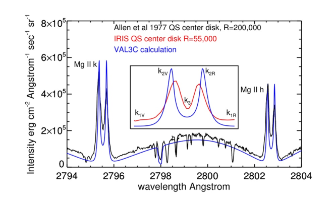
Figure 1.— The figure shows observed and computed profiles of the Mg II $h$ and $k$ lines for quiet Sun conditions close to disk center. Calculations were made with a full treatment of partial redistribution using the code RH (Uitenbroek, 2001). The inset shows the $k$ line with notations for the $k_{1}$ minima, $k_{2}$ maxima, and $k_{3}$ minimum in intensity, discussed in the text. The present paper focuses on the systematic discrepancies between observation and theory at wavelengths between the maxima, such as the $k_{2}$ peaks shown for Mg II. These generally lie less than 0.30 Å from line centers, of profiles of the resonance lines of H I, Mg II, and Ca II, the strongest lines in the solar spectrum.

In the second problem, the centers of line cores ($k_{3}$ in the figure), controlled by CRD, were computed to be too dim by factors of several, relative to the $k_{2}$ peaks. These discrepancies remain today for some of the strongest lines in solar and stellar spectra, including H L$\alpha$, and to a lesser extent L$\beta$ (Gouttebroze et al., 1978; Basri et al., 1979); the Mg II $h$ and $k$ lines (Vernazza et al., 1981); the Ca II $H$ and $K$ lines (Lemaire et al., 1981).

Observed profiles of these strong lines were recognized to be asymmetric. The explanation proposed early concerns the relative bulk motion between the middle and upper chromosphere (Athay, 1970), a result compatible with the upwardly-propagating radiating shocks calculated in 1D models by Carlsson & Stein (1995). This remains a related problem of interest here, but we do not address it directly here.

More sophisticated calculations based upon 3D radiation-MHD (R-MHD) models computed with the Bifrost code (Gudiksen et al., 2011) have reduced core $k_{3}/k_{2}$ Mg II intensity ratio discrepancies somewhat (Sukhorukov & Leenaarts, 2017), and also for the $K_{3}/K_{2}$ Ca II ratios (Bjørgen et al., 2018). But issues in line cores remained, in particular they found that observed peak separations implied that something was missing in their models.

Physically, the cores of the strong lines generally correspond to wavelengths where Doppler-shifted thermal and other motions control the opacity and source function. Therefore in this “Doppler core”, CRD is a reasonable approximation. While the Doppler broadening widths are not known a priori, the cores are considered to span about 3 times the r.m.s. Doppler width, before both opacity and source function become controlled by coherent scattering. In models and observations, this 3$\times$Doppler width varies systematically from $\pm 25$  km s^-1 for heavy elements such as calcium, to $\pm 50$  km s^-1 for hydrogen.

Given the importance of strong lines to the chromospheric energy balance, the onset of the solar corona, the irradiance effects in the solar system and the recent work on the Hanle effect in the cores of these lines (see, for example, Ishikawa et al., 2018), we re-analyse various models and data-sets to understand better the meaning of the remaining discrepancies between observation and models.

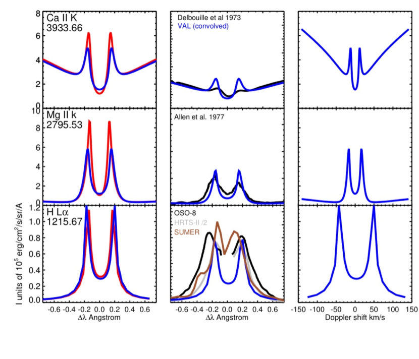
Figure 2.— The figure shows the resonance lines of Ca II, Mg II and H I, for two sets of calculations in model 3C of Vernazza et al. (1981). The blue lines use the micro-turbulence values taken from the model. Red lines show calculations using a micro-turbulence with a maximum of 1  km s^-1. Calculations were made with a full treatment of partial redistribution using the code RH (Uitenbroek, 2001). The middle panels compare the calculations convolved with instrumental profiles. For the L$\alpha$ line the computed profiles were convolved with the OSO-8 profile. The rightmost panels show computations for VAL3-C plotted on a Doppler scale.

The early 1D models remain a reasonable first physical approximation because of steep hydrostatic stratification, where the dominant direction of transfer of radiative energy lies in the vertical direction (e.g. Judge, 2017). However, even though in the 3D R-MHD models the stratification is steep (isobars are more horizontal than vertical), there are many conditions where, owing to magnetic and Reynolds stresses evolving in response to convection beneath, the effects of horizontal radiative transfer are important. Thus we study 1D and 3D models, focussing on the differences arising between 1D formal versus 3D formal solutions. Our attention is focused on the resonance lines of H I, Mg II and Ca II.

Lastly, a unique study by Bocchialini & Vial (1994) reported simultaneous spectra acquired with various $1\arcsec$-wide image-plane slits and different spectrograph exit slits, in the resonance lines of H I, Mg II and Ca II, from the LPSP instrument on the OSO-8 satellite. They found that, while Mg II and Ca II data were similar, the L$\alpha$ data appeared qualitatively different.

2. Statement of the problem

Figures 1 and 2 illustrate our core problem of interest: the calculated profiles have ratios between peak and core brightness that systematically exceed observations, even those with spectral resolutions of 200,000, by a factor of 1.5–2. Below we will examine in detail data of Mg II from the Interface Region Imaging Spectrograph (IRIS, De Pontieu et al., 2014) and from calculations which highlight spatially-resolved spectra in contrast to the comparison of spatial averages shown.

Armed only with 1-dimensional calculations, early resolutions that were proposed to this problem were necessarily limited. Within each calculation, the only option is to examine the assumed velocity fields within the chromosphere. If included as a formal “microturbulence” (random fluid velocities exist on scales below the photon mean free path), the effect is to increase the wavelength differences between the intensity peaks. As shown in Fig. 1, the separation-of-peaks for the $h$ and $k$ lines in standard 1D calculations are close to spatially-averaged observed values. The well-known effect of variations in micro-turbulence is recalled in Figure 2. (Curiously, using the distribution of micro-turbulence of VAL3-C, the peak intensities are split by similar amounts in wavelength, yet the line center wavelengths are in the ratio $1:2.3:3.3$).

Another option in 1D modeling is to include line broadening as macro-turbulence, then within each 1D calculation, the velocity would be introduced as a macroscopic, not microscopic flow. In this case, the emergent profiles, for changes small in magnitude compared with micro-scale motions, introduce shifts (and asymmetries if velocity gradients exist) of the entire core profiles. This resolution, proposed by earlier authors (e.g. Gouttebroze et al., 1978), suggests that each observation sums spatially over intensities from several such adjacent atmospheres in each pixel. Figure 3 shows a schematic picture of this proposed solution. Each atmosphere is a 1D solution to the non-LTE equations. If each observation corresponds to a superposition of a set of 1D calculations that are randomly distributed in line of sight velocity, to some degree the differences can be reconciled. Each observation then corresponds to the simple sum of individual theoretical profiles, each shifted in wavelength according to a bulk velocity shift.

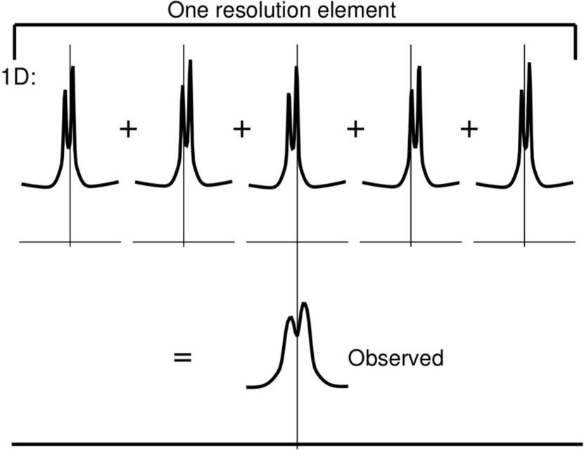
Figure 3.— A schematic picture of the “macroturbulent” explanation for the reduced peak-core intensity contrast in chromospheric resonance lines. Each profile in the upper panel comes from an unresolved individual atmosphere computed in 1D, having a large peak-core ratio (Figure 2). In the macro-turbulent picture, these profiles presumed to be shifted in wavelength by an amount comparable to the core-peak wavelength difference. The sum of these unresolved profiles yields the profile labeled “Observed”.

Spectroscopic turbulence was studied in the context of 1D models by Carlsson & Scharmer (1985). They found that the regimes of applicability of the micro- and macro- turbulent limits were found to be ${<}25$ km and ${>}3000$ km respectively, using velocity fields with a variety of correlation lengths, for lines of Ca II. These lengths can be compared with a photon mean free path of 120 km and thickness of the entire stratified chromosphere of 1500 km. They showed that typical profiles could not be explained by a linear combination of micro- and macro-turbulent flows.

Three-dimensional radiation-MHD (R-MHD) models (Sukhorukov & Leenaarts, 2017; Bjørgen et al., 2018) are based not on ad-hoc explorations, but are solutions to the dynamic equations of motion and radiative transfer. They are performed on grids fine enough to avoid too much dissipation, but for which solutions can be obtained in reasonable computing time. The calculations examined here have grids with spacings of 49 and 34 km horizontally and vertically respectively, and are therefore capable of exploring radiative transfer in different regimes of spectroscopic turbulence to the extent that their intrinsic numerical smoothing permits significant changes in velocities to occur between neighboring slices through the 3D atmosphere which determine the opacities and source functions. These calculations were advanced in time using radiation transfer solutions based upon the short-characteristics method, which is encumbered with a large, unphysical diffusion. The source functions for strong lines are dominated by scattering. As such, the modeled profiles, even computed with long characteristics, must be treated with some caution. Our final goal is to explore how profiles of strong lines computed with the best 3D MHD models compare with these observations.

3. Observations and their analyses

3.1. Typical quiet Sun line profiles

First, we examine the highest dispersion spectra of the three lines from the literature, of the quiet Sun, but with low spatial resolution. Figure 1 shows data of both the $h$ and $k$ lines from a $7\arcsec\times 130\arcsec$ area of the quiet Sun (Allen et al., 1977). Figure 2 shows profiles from regions of quiet Sun, highlighting the cores of Ca II, Mg II and H I resonance lines, from several instruments. The figure compares the observations with calculations from the 1D VAL-3C model. Spectra of Ca II lines were taken from the atlas of Delbouille et al. (1973). The spectrometer used had a native spectral resolution of ${\cal R}=600,000$, so that instrumental broadening is negligible. The Mg II spectra are taken from the ${\cal R}=200,000$ quiet Sun spectra shown in Fig. 1 (Allen et al., 1977). Solar data for H I L$\alpha$ are all of a significantly lower spectral resolution. Those obtained from rocket flights or low Earth orbit are also affected by absorption by neutral hydrogen in the Earth’s upper atmosphere in the line core. These include data from the HRTS-II experiment from Brekke et al. (1991) with ${\cal R}=24,000$ and the LPSP instrument on OSO-8, which obtained quiet Sun spectra with ${\cal R}=60,000$. Data from the SUMER instrument on SoHO have a lower spectral resolution of 15,000, even though the instrument, on the SoHO spacecraft at the L1 Lagrange point, is unaffected by the geocorona. L$\alpha$ SUMER data also have been obtained, mostly behind a mesh at the edge of the detector, to avoid saturation. Curdt et al. (2008) obtained SUMER L$\alpha$ data behind the partially-shut door of the telescope, of six quiet-Sun regions on June 24–25, 2008. Owing to the apodization of the pupil plane by the partly-closed door, the angular resolution is difficult to assess, but they found the characteristic asymmetry (blue peak brighter than red) which increased with brightness. The central core was found to be typically 75% of the brightness of the blue peak, independent of limb distance, at a spectral resolution of 15,000.

Quiet Sun L$\alpha$ profiles from all three instruments are compiled in the lower middle panel of Fig. 2. The SUMER data shown there are from Curdt et al. (2001). All three lines show similar qualitative differences with 1D calculations. 1D calculations tend to predict brighter peaks and a darker central intensity.

A closer look at Figures 2 and 3 immediately yields tight constraints on any macro-turbulence. The right-most panels of Fig. 2, plotted against Doppler velocity, show that the Ca II $K$, Mg II $k$ and H I L$\alpha$ line cores would need systematically different macroturbulent velocity distributions to explain the observed core-peak intensity ratios. The Ca II $K$ line would require r.m.s. speeds of 10  km s^-1, but Mg II $k$ and H I L$\alpha$ would need r.m.s. values of 30 and 50  km s^-1 for the superposition shown in Fig. 3 to work. In stratified atmospheres, these three line cores form all within a region termed the “upper chromosphere” (see, for example, Fig. 1 of de la Cruz Rodríguez et al., 2019 and Fig. 3 of Štěpán et al., 2015). We note that the area coverage of spicules inferred from data above the limb is too small to contribute significantly to the spatially-averaged profiles, (e.g. Judge & Carlsson, 2010; Mamedov et al., 2016). However, models do show that the $k_{2}$ and $K_{2}$ peaks form substantially lower in the atmosphere (Vernazza et al., 1981; Leenaarts et al., 2013; Bjørgen et al., 2018).

The 3D models have revealed that the peak separations of these lines can increase in locations where the chromospheric temperature rise is located deep in the atmosphere (see Fig. 20 of Bjørgen et al., 2018). But, no matter the details of the complex non-LTE formation of these lines, we know of no first-principles reasons nor data that are compatible with the idea of a systematic gradient of macro-scale motions that can rescue the explanation that the peak-to-core ratios are small because of macro-turbulence. Indeed, below we show that the line profiles of Mg II lines obtained with the IRIS instrument, obtained with a high cadence and at the highest angular resolution ever achieved, also can be used to reject this hypothesis.

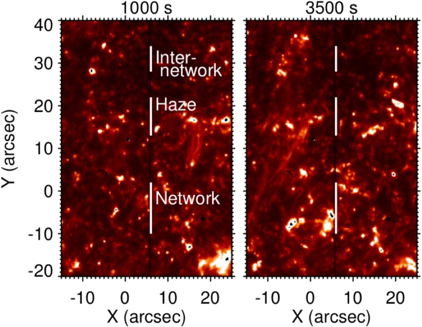
Figure 4.— Slit-jaw images from the 1400 Å channel are plotted to over-expose the brightest pixels, revealing bright regions associated with continuum UV emission formed in the chromospheric network. The two frames correspond to the times shown on the $y-$axis of the slit spectra (Figure 5).

3.2. Quiet Sun Mg II line profiles in time and space

We examine detailed profiles for the Mg II $h$ and $k$ lines from the IRIS instrument (De Pontieu et al., 2014). While IRIS does not measure the UV spectra at the highest spectral resolution, the linear properties of the detector combined with the high angular resolution make it uniquely suited to address the problem of interest. Measurements in the Mg II $h$ and $k$ lines have a spatial step along its slit of $0.168\arcsec$, a critical sampling of the angular resolution of $0.33\arcsec$. Inspection of typical data (e.g. Figure 5 of De Pontieu et al., 2014) suggests that quiet regions have only modest significant spatial variations of the $k_{2}$ and $h_{2}$ peaks observed along the projected spectrograph slit, as seen at the nominal angular resolution of IRIS. The center-limb behavior shown in Fig. 6 of De Pontieu et al. (2014), reveals that peak separations first increase, and finally disappear some $5\arcsec$ above the limb seen in the neighboring continuum. The line profiles become a narrow single peak $5\arcsec$ higher.

All of the IRIS data were reduced to photometrically-calibrated spectra using the IDL SolarSoft packages as well as deconvolved with the point spread function (PSF) of the IRIS telescope, which has been measured during a Mercury transit by Courrier et al. (2018).

Quiet Sun Mg II data were obtained with IRIS close to disk center beginning on February 27, 2014, at 5:39:28.850, in a “sit and stare” mode. 290 frames of 774 0.16635$\arcsec$-wide pixels (solar $y$) by 554 0.0254 Å-wide wavelength pixels. We will focus on spectra, but simultaneous IRIS slitjaw images were obtained in the 1400 Å channel. Figure 4 shows examples of these images obtained 1000 and 3500 seconds into the time-series. Each has been median-filtered over time (90 seconds) to remove internetwork oscillations and fast dynamics in the low-density transition region.

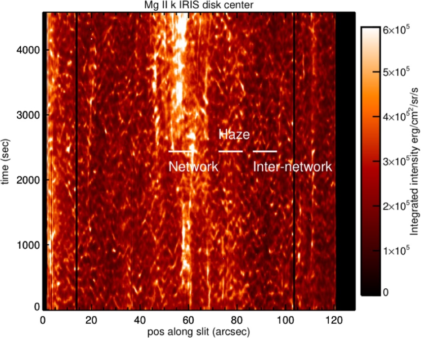
Figure 5.— The wavelength-integrated intensity of the core of the Mg II $k$-line is shown as a function of position along the IRIS slit and time, highlighting areas of network and inter-network. The area marked as “haze” is an intermediate region, perhaps with some intensity contributions from high-lying chromospheric fibrils.

The thick lines show three regions we highlight below: network, haze, and inter-network. The color table saturates the highest DN to reveal UV continuum emission that forms in the lower chromosphere.

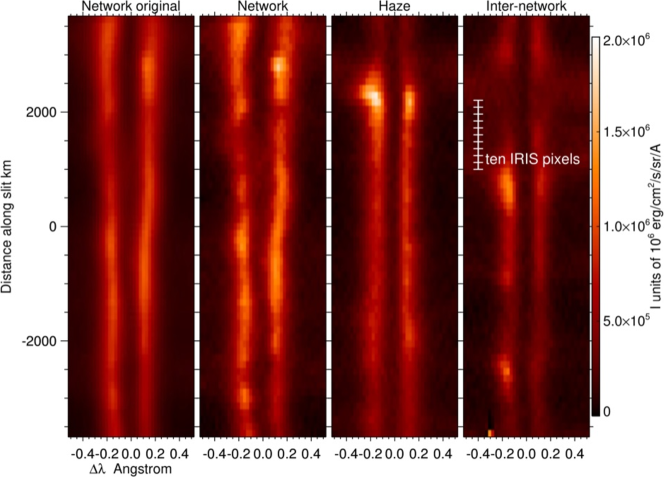
Figure 6.— Line core profiles of Mg II $k$ are shown as functions of wavelength from line center and position along the IRIS slit for the middle exposure of the time series. The left-most panel shows original data, the three right panels have been spatially de-convolved using the prescription of Courrier et al. (2018). The profiles are taken from the slit positions and time corresponding to the white lines shown in Fig. 5.

Figure 5 shows wavelength-integrated intensities of the Mg II $k$ line core, spanning 1 Å (roughly the wavelength separation between the $k_{1}$ minima), as a function of position along the slit and time. The data were acquired with a cadence of 16.8051 seconds, for a total duration of 81 minutes. The total solar area rotating under the fixed slit was therefore roughly $13\arcsec\times 120\arcsec$ (solar $x$ and $y$ respectively). This area covers 1 part in 2000 of the area of the solar disk, below (Section 3.5) we therefore examine a larger region.

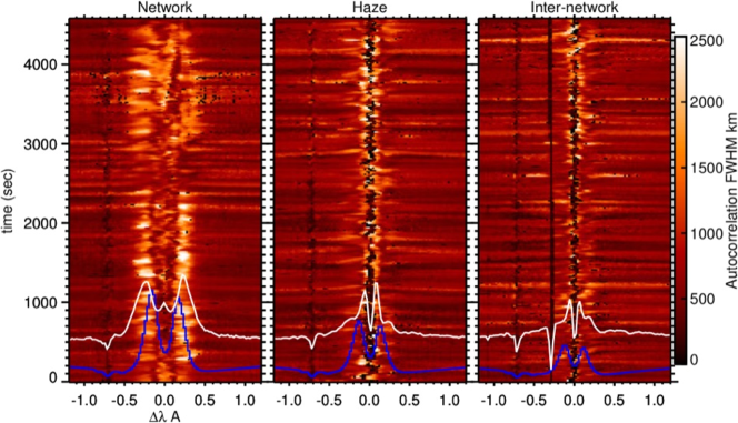
Figure 7.— The spatial auto-correlation full-widths of the three regions (Figure 5) are shown as images as a function of wavelength and time, each “image pixel” has the correlation length shown on the color bar to the right. The correlation lengths shown were averaged over the three regions: network, haze and inter-network in Fig. 5. The white line plots autocorrelation FWHMs also averaged in time along each column, the time scale in seconds on the left applies to the FWHM widths measured in km. The blue lines show, for reference, the average line profiles along the same columns, divided by $10^{3}$ (i.e. multiply the $y$-values in blue by $10^{3}$ to get physical intensities in erg cm^-2s^-1sr^-1Å^-1). There is a dark pixel at $-0.3$ Å in the internetwork region, the other features are solar.

The data, when deconvolved, have a sufficiently high angular resolution ($0\farcs 33$) that the macro-turbulent picture can be directly addressed. Each resolution element (two pixels) corresponds to about 240 km on the solar surface. If a superposition such as that shown in Fig. 3 were responsible for filling-in the line cores, then some profiles adjacent in space should exhibit large variations between separate resolution elements, i.e. on scales down to 240 km. But such variations are absent, as shown in the typical, randomly chosen samples of line profiles of network, inter-network, and a hazy intermediate region. These profiles are typical of the entire data-set, including the $h$-line.

3.3. Spatial auto-correlations

The leftmost panel of Figure 6 has not been spatially de-convolved, the others have. The tick-marked line in the rightmost panel shows ten spatial pixels, each of which critically sample the convolved data. Very little structure below scales of about 5 pixels ($\equiv 600$ km) is visible. This figure prompted us to measure quantitatively the spatial structure along the slit of the entire dataset, using auto-correlations. Thus, we computed the spatial auto-correlation lengths along the IRIS slit at each wavelength, and time, for those columns in Fig. 5 corresponding to all three marked regions.

The figures below show autocorrelation lengths of the intensity images $I_{\lambda}(y)$, which are the characteristic full-widths at half-maximum (FWHM) of the functions

$$c_{\lambda}(\ell)=I_{\lambda}(y)\cdot I_{\lambda}(y+\ell),$$ (1)

centered on the maximum ($\ell=0$). Since $c_{\lambda}(\ell)$ depends on each wavelength $\lambda$ across the line profiles, any variations of line-of-sight velocity on resolvable scales will be reflected by changes in the monochromatic intensities on the same length scales, thereby imprinting the velocities onto these correlation lengths. Figure 7 shows these $c_{\lambda}(\ell)$ values. Over-plotted is the average line profile in blue, and the autocorrelation FWHM lengths averaged over space and time, in white, along the network, haze, and inter-network slit regions.

Small values of the FWHM of $c_{\lambda}(\ell)$ correspond to rapid changes in space, and vice versa. An obvious feature of Fig. 7 are that in the wings of the $k$ line ($\lambda$ outside of the $k_{1}$ minima) the three regions are not easily distinguishable, unlike the line cores which are radically different. There are some extended periods where the structure in the wings of the network contain consistently small FWHM values (between 1400 and 1600, or 1800 to 2200 seconds for example), these upper photospheric signatures behave, statistically at least, in a similar fashion. The average autocorrelation lengths outside of line cores are all close to 400 km (the averages are shown as white lines in the figure).

But within the cores, the network and other regions behave quite differently. The average intensity profiles in the haze and internetwork regions are similar in shape to the average correlation length profiles (white and blue lines). But in the network, the very cores of the autocorrelation profiles possess a peak at the $k_{3}$ core that is absent in the intensity profiles. The spatial autocorrelations are also larger farther from line center ($\Delta\lambda>0.1$ Å in the network region, with the exception of a short period around $t=2600$ seconds (left panel of Fig. 7). During the first half of the time series autocorrelation lengths can exceed ${\approx}2500$ km near the $k_{2}$ peaks, and almost symmetric about line center. Later, after about 3000 seconds the region of network shows an asymmetric autocorrelation profile in wavelength, line cores lengths exceeding 2000 km, but with a coherent darker feature, i.e. smaller lengths between 0.1–0.2 Å to the red of line center (Doppler redshifts of 10 and 20  km s^-1) between 3200 and 4300 seconds.

All three regions have average spatial scales exceeding 800 km at all wavelengths which have significant core emission (within about ${\pm}0.3$, 0.2, and 0.1 Å respectively for the network, haze, and internetwork). The spatial auto-correlations within the cores (${\pm}0.5$ Å) have structures with a median of 1060 km, mean of 1140 km, and r.m.s. variation of 440 km, for the haze and internetwork data, with 20% higher typical values for the network.

In contrast, the haze and internetwork regions possess a significant and persistent dark streak within 5–8  km s^-1 (Doppler shift) of $k_{3}$. There, the spatial FWHM correlation lengths fall to 400 km, which is only about twice the spatial resolution of IRIS. We will speculate on the origin of these small structures below.

In summary, these IRIS data reveal that:

1. Away from the line cores (outside $k_{1}$ minima), all regions have autocorrelation FWHM values close to 400 km, roughly twice the IRIS resolution.

2. At and near wavelengths of intensity maxima ($k_{2}$), FWHM measurements exceed 1000 km, increasing to over 1500 km in network regions.

3. Outside of network regions, $k_{3}$ has a persistent small spatial FWHM of $\approx 400$ km, seen only in line center pixels and those two immediately to the red side (${\leq}10$  km s^-1 from line center).

4. Over network regions, autocorrelation lengths are systematically larger, extend further in $\Delta\lambda$, and have a broad minimum near 800–900 km across the central ${\pm}0.2$ Å. Within ${\pm}0.1$ Å the lengths increase producing a third, central small peak in average autocorrelation profiles.

To explain the small $k_{3}/k_{2}$ ratios, the macro-turbulent picture requires large changes in line-of-sight velocities on scales down to the 200 km resolution limit of IRIS. Our analysis of typical IRIS data for Mg II rejects this hypothesis.

3.4. Other relevant observations

Other spectral lines have been observed at a high angular resolution which can also shed light on conditions where the cores of strong solar resonance lines form. Spin-forbidden lines of O I at 1356 and 1358 Å have been observed repeatedly with UV spectrometers. The lines are optically thin across most of the chromosphere, the shared upper level is 9.15 eV above the ground level of O I. The O I ionization is strongly tied to the H I level populations through a well-known resonant charge-transfer reaction, and so excitation by collisions with electrons will occur under conditions common to these lines of O I and L$\alpha$, whose upper level lies at 10.19 eV. Naturally, the L$\alpha$ line source function and emergent intensity are dominated by photon scattering, unlike the spin-forbidden lines of O I. But the two lines otherwise are excited under similar conditions within the chromosphere.

The HRTS instrument has provided spectra near 1350 Å at a spectral resolution (50 mÅ) similar to IRIS, but a lower spatial (1$\arcsec$) resolution. HRTS data analyzed by Athay & Dere (1989) show that this line’s kinematics is unspectacular, with r.m.s. Doppler shifts of 2  km s^-1, and linewidths close to that of the instrument. The unresolved motions are at most 40% of the sound speed, which is 10–15  km s^-1. It seems there is little power in motions, resolved or unresolved, across the quiet Sun’s upper chromosphere. Carlsson et al. (2015) reported widths of ${\sim}7$ km s^-1of the O I 1356 Å line in IRIS data in quiet and plage regions. Optically thin lines such as the 1356 line have contributions from many scale heights across the chromosphere, so their line widths reflect the line-of-sight sum of many different heights.

3.5. A broader sample of Mg II IRIS data

The above IRIS dataset was selected to represent a typical quiet Sun region at disk center. But these data sampled just 1 part in 2000 of the solar surface. We therefore looked at statistical properties of the IRIS Mg II $h$ and $k$ profiles from a spatial (raster) scan, that of April 15, 2014, between 05:25:24 and 05:43:28 UT. This spanned an area of $127\arcsec\times 119\arcsec$, which is ten times larger than the sit-and-stare observation.

This observation included a little more active Sun, lying at the periphery of a substantial active region (NOAO 12036). We found that only about 10% of the line profiles had $k_{2}/k_{3}$ intensity ratios between 4 and 6, spanning the value of ${\approx}5$ for the VAL3-C calculation. The bright chromospheric network showed no more spatial correlation with these deep line ratios than other pixels in the instrument’s field of view. On balance, these data from a larger area confirm that large $k_{2}/k_{3}$ intensity ratios above 4 are present at a 10% level. The median ratio is 2.5.

4. Re-analysis of recent 3D calculations

We have examined model data from Sukhorukov & Leenaarts (2017) and Bjørgen et al. (2018). The atmospheric structure in the models is the same in both articles and is determined by R-MHD calculations, using the short characteristics method to solve for radiation gains and losses in the energy equation. After the calculations have been evolved, the authors then studied solutions to the transfer equation using long characteristics for the 1D and 3D calculations. Here we focus on the computations for the $k$ line by Sukhorukov & Leenaarts (2017), and also comment on those for the Ca II $K$ line at 393.4nm. Our purpose here is to examine the hypothesis that the line cores of chromospheric resonance lines are filled in by horizontal radiative transfer.

The horizontal component of the numerical grid has pixels of width 47 km. While the MHD calculations upon which these radiative transfer calculations are based are themselves highly diffusive compared with the real Sun, the thermal structure in their calculations nevertheless has features down to these scales. The computational data analyzed here have been re-binned to scales half of the native resolution, 98 km in the horizontal direction. This scale is comparable or smaller than typical photon mean free paths through the stratified chromosphere. While a finer grid is desirable, these calculations are fine enough to reveal the effects explored below.

The modeled region is similar to enhanced network on the Sun, with an unsigned magnetic field strength of 50 G passing through the photosphere (Carlsson et al., 2016; Sukhorukov & Leenaarts, 2017; Bjørgen et al., 2018). A typical snapshot of a time-dependent 3D calculation is taken. From the source functions in each voxel, the long-characteristic method is used to produce the emergent intensities, including PRD. Therefore the solutions shown are a kind of hybrid: the source functions and the optical depth scales are computed using the diffusive short-characteristic method, but the final emergent intensities, given these parameters, are far less diffusive.

Figure 8 shows emergent intensities from a small part ($6\times 6$ Mm²) of the calculated area ($24\times 24$ Mm²), using the long characteristic method, for a region at disk center ($\mu=1$). When compared with observations, we note firstly, that the computed features $k_{2V}$ and $k_{2R}$ are factors of between one and two brighter than the average quiet Sun data shown. This is to be expected given the higher concentration of the magnetic field used in the computations. But the $k_{2}/k_{3}$ contrasts are also significantly higher, both in 3D and 1D, and the $k_{2V}$ and $k_{2R}$ separations are smaller than observed. Qualitatively similar results (from Bjørgen et al., 2018 but not shown here) are seen for the Ca II $K$ line, where the average $K_{2R}$ and $K_{2V}$ peaks are separated by 0.33 Å in both quiet and plage regions (compare Figures 3 and 5 of Linsky & Avrett, 1970), whereas the average over the computed enhanced network region is about half of this (0.17 Å).

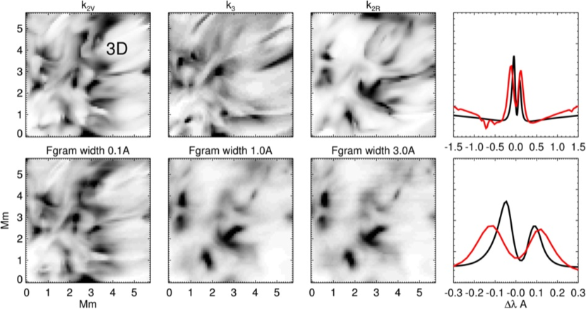
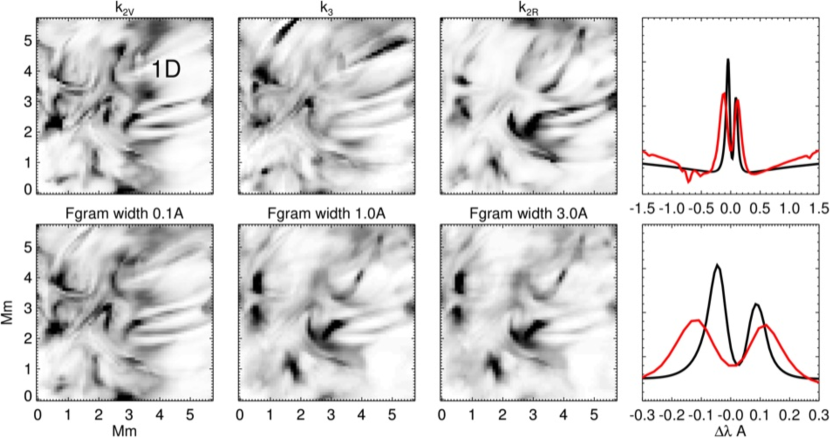
Figure 8.— Images in the Mg II $k$ line computed by Sukhorukov & Leenaarts (2017) are shown at the computed $k_{2V}$, $k_{3}$ and $k_{2R}$ wavelengths (rows one and three), and through a filtergram instrument with the widths indicated. The gray scale is linear from zero to $3.8\cdot 10^{6}$ erg cm^-2s^-1sr${}^{-1}\AA^{-1}$, reversed (black is the maximum intensity) to reveal fainter emission between bright regions. The rightmost panels show the average spectra (black) superposed with the average quiet Sun from the IRIS data studied here in red. Although the R-MHD calculation is for a region of network, the region is dominated in area by non-network emission, thus we compare with the quiet IRIS data. Note that the computed line $k_{2}$ peak separations are substantially smaller than observed.

Significantly, in comparison with plage observations, these $k_{3}$ and $K_{3}$ components are far deeper in the computations. This suggests that the source function is on average larger where this feature is formed than is captured in the calculations.

In Figure 9 we show spatial auto-correlation data computed from the 3D and 1D intensities of the $k$ line, together with spatially-averaged intensity profiles. Solid lines show observations, dashed lines computations. The auto-correlation characteristic lengths show three kinds of behavior depending on the wavelengths relative to line center. In the line wings, the images have the smallest spatial scales, with FWHM values of about 750 and 610 km. In 3D, these scales steadily increase towards the line cores, peaking near the observed peaks $k_{2V}$ and $k_{2R}$. (In 1D these lengths decrease towards the line center before showing a small increase at $k_{2V}$ wavelengths). Within the line core, the widths computed in 3D drop dramatically to below 700 km.

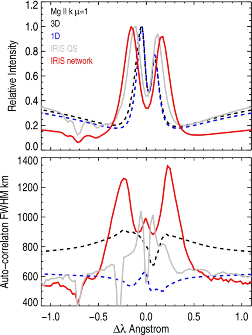
Figure 9.— Average profiles (top panel) are shown with auto-correlation full-widths for the IRIS network and quiet regions (red and gray respectively) in the lower panel. The same data for the 3D and 1D calculations of Sukhorukov & Leenaarts (2017), are also shown as dashed lines.

The comparison of 3D and 1D images in Fig. 8 is instructive in ways complementary to the interesting points made by Bjørgen et al. (2018). Figure 9 shows clearly that 3D transfer effects are important within $\pm 1$ Å of line center: the FWHM length scales are larger on average by a factor of two for the $k$ line (15–20% for the $K$ line) in 3D than 1D. The 3D features all appear “fuzzier” to the eye than their 1D counterparts, on scales of a few hundred kilometers in Fig. 8. We will speculate further on what is missing in these calculations in Section 5.

The second and fourth rows of Fig. 8 show how the calculated model might be observed through filter instruments, with FWHM values of 0.1, 1, and 3 Å. Wider FWHM instruments have been used in solar physics for many years to record the Ca II lines, and other, narrower filter widths have been developed. These panels suggest that 3D smearing effects are biggest at wavelengths within the emission cores. The differences are probably lower limits, given that the source functions for strongly scattering lines are smeared by the use of the short characteristics, which will tend to underestimate differences between the 1D and 3D formal solutions to the transfer equation.

5. Discussion

We have re-visited an old problem concerning the upper chromosphere of the Sun: is there a clear discrepancy between observed and computed profiles in the Doppler cores of the strongest lines? If so, can we determine its origin? Firstly, we compiled data to re-examine literature from the 1970s when this problem was first addressed. Using these data, including optically thin lines generated in the same regions as the strong lines, we confirmed earlier work showing that micro-turbulence cannot account for the systematic behavior of the data and argued that macro-turbulence also fails. On this basis, we then examined the $k$ line of Mg II in detail, taking advantage of the quality and angular resolution of the IRIS instrument. We then explored radiation MHD simulations of an enhanced network region of the $K$ line of Ca II. In particular, we compared the line cores in 1D and 3D to explore the effects of horizontal radiative transfer on the emergent spectra generated throughout the chromosphere.

Our first conclusion is that the small peak-core ratios in these resonance lines cannot be due to turbulence on any scale. Given the well-known result that micro-turbulence serves mostly to increase the separation of peaks (see Fig. 2), our conclusion rests on the refutation of macro-turbulence. Three lines of argument all point to this result.

• The macro-turbulence limit requires the spatial averaging of profiles of fluid elements, which are Doppler-shifted by a velocity distribution, which spans the computed 1D separation of peaks. If the distribution were narrower, little difference would be seen between the 1D and average profiles. If larger, then we would see multiple peaks for a small number of averaged elements, and/or a severely broadened feature. But observations clearly show a steady increase of separation of peaks from Ca II to H I by a factor of three in Doppler shift. Yet the deep cores of these features all form within the confines of the upper chromosphere and higher. Whether or not the chromosphere is thermally isolated from the corona above by mostly horizontal magnetic fields, these line cores likely form in regions of very steep gradients in electron temperature where ionization causes them to become optically thin.

• Optically thin UV lines observed with the HRTS instrument since the 1970s also have contribnutions from the upper chromosphere. Spin-forbidden lines of O I near 1356 Å require almost the same population of electron energies to be excited as H L$\alpha$, yet they are spectrally unresolved by HRTS and show small subsonic deviations of just a few  km s^-1 along the instrument’s slit (e.g., Athay & Dere, 1989).

• Spatially de-convolved profiles of the Mg II resonance lines observed by IRIS show very few features smaller than 600 km along the slit, yet the spatial resolution is close to 240 km (Figures 6 and 7). Between the $k_{1}$ minima, average autocorrelation lengths vary between 800–1200 km, larger values being seen in brighter regions of the network.

For our second conclusion, based upon differences between the 1D and 3D autocorrelation calculations (Figure 8), at least some of the peak-to-core ratio discrepancy is due to horizontal components of radiation transfer. Figures 8 and 9 unambiguously reveal the small-scale smearing effects of horizontal radiative transfer in the emergent intensities. Horizontal radiative transport in space is the most likely way to explain the difference between the 1D and 3D calculations. These differences cause the lowering of contrast across the line profiles in both space and frequency, and larger the autocorrelation lengths in space.

We can also draw a third conclusion, namely that the upper chromosphere may well harbor less “turbulence” than previously thought. The profiles of the three strongest lines formed in this region simply do not support supersonic motions within the uppermost layers of the stratified atmosphere for the vast majority of the time. In this picture, supersonic spicules and other features simply are not abundant enough and do not cover enough area of the surface to be significant, on average, in affecting these line profiles.

5.1. Further speculations

Beyond these conclusions, the confrontation between computed and observed profiles necessarily becomes more speculative. Arguably, modern MHD calculations capture the lower chromosphere better than the upper chromosphere and higher layers. After all, the energy in higher layers is modified and filtered by its propagation and dissipation through the lower layers, which themselves remain a subject of active research. The interface between the cool chromospheric and hot coronal plasma is not only difficult to model accurately, but observations over the past century have consistently revealed the complex thermal nature of the fine structure of the upper chromosphere. Even the latest radiation MHD calculations attempting to understand why the Sun must produce spicules are based not on 3D but “2.5D” calculations in which special symmetries are imposed (Martínez-Sykora et al., 2018). It remains premature to state that we really know what spicules, and other products of the plasma dynamics of the chromosphere extending higher up, really are.

These and other structures entirely absent in 1D calculations and 3D calculations may well influence in our analysis. As made explicit by Judge et al. (2015), such structures can have optical depths and source functions radiatively de-coupled from the chromosphere beneath. These structures will simply absorb or emit radiation along the line of sight on their physical scales, essentially disconnected from the non-locally coupled radiative transfer solutions leading to the bulk of the line profiles beneath. They can have structure on scales much smaller than the photon path lengths. Owing to the magnetic control of these plasmas owing to lower densities and pressures, they might appear at almost any Doppler shift up to the (high) Alfvén speed. Thus we might expect to see absorbing and/or emitting structures perhaps with length scales down to the diffraction limit if such structures cover much of the chromosphere much of the time. This kind of picture might explain the peculiar structures seen in the network panel in the upper part of Fig. 7. In the internetwork and haze regions, we see the smallest structures in the line cores, mostly within $\pm 0.05~{}\text{\AA}\equiv\pm 5$  km s^-1 Doppler shifts (Figure 7, seen in the images and the column-averaged white lines). These are sub-sonic speeds. Super-sonic motions associated with spicules and some fibrils are notable by their absence. For a typical length of a spicule of 5–10$\arcsec$, and assuming that $10^{5}$ such spicules are present at any time on the Sun (Mamedov et al., 2016), we would expect to see one spicule cross a randomly oriented slit of this length at any time. The small-scale features at line-center observed almost everywhere are therefore not related to spicules. Interestingly, similar features are present in the numerical models for the Ca II $K$ line, outside of the chromospheric network.

Finally, as noted earlier, if the location of the chromospheric temperature rise is deeper in the atmosphere than typical models suggest (see Fig. 20 of Bjørgen et al. (2018)), then this problem should be re-visited. Hints of a potential contribution of such a regime to a new understanding are present in line widths computed from A–F models in Vernazza et al. (1981), and the calculations of Carlsson et al. (2015). This is beyond the scope of the present paper but will be addressed in future.

6. Conclusions

Our results listed above suggest that the amount of “turbulence” present in the upper chromosphere has been over-estimated in prior work. This may have significant consequences for the energy budget that can be used to heat the overlying regions of the solar atmosphere.

Our analysis is incomplete in many ways: for example, we have no pure solar spectra for H L$\alpha$ with sufficient spectral resolution and photometric quality to make comparisons with computations; neither have we any images with sufficiently narrow passbands (Doppler widths ${\mathrel{\hbox to0.0pt{\lower 3.7pt\hbox{$\sim$} \hss}\raise 1.7pt\hbox{$<$}}}10$  km s^-1) to be able to compare with predictions from computations including scattering such as in Fig. 8. Even so, it is clear that the various models in 3D as well as 1D are missing essential physical processes affecting the typical conditions in the upper solar chromosphere.

The consequences of revisiting of early work remain to be fully understood. There are many observations relevant to this study, such as the remarkable images of broad-band L$\alpha$ light from the VAULT instrument (e.g. Patsourakos et al., 2007), of chromospheric fine structure in very narrowband images in H$\alpha$, the Ca II infrared triplet lines and others (e.g. Lipartito et al., 2014). Our work is almost certainly important in terms of the amount of energy stored in and transported by the small-scale mass motions that we need to invoke, as well as 3D transfer effects, to help explain the problem we have addressed.

References

- Allen et al. (1977) Allen, M. S., McAllister, H. C., & Jefferies, J. T. 1977, NASA STI/Recon Technical Report N, 78
- Athay (1970) Athay, R. G. 1970, Sol. Phys., 11, 347
- Athay & Dere (1989) Athay, R. G., & Dere, K. P. 1989, ApJ, 346, 514
- Ayres & Linsky (1976) Ayres, T. R., & Linsky, J. L. 1976, ApJ, 205, 874
- Basri et al. (1979) Basri, G. S., Linsky, J. L., Bartoe, J.-D. F., Brueckner, G., & van Hoosier, M. E. 1979, ApJ, 230, 924
- Bjørgen et al. (2018) Bjørgen, J. P., Sukhorukov, A. V., Leenaarts, J., et al. 2018, A&A, 611, A62
- Bocchialini & Vial (1994) Bocchialini, K., & Vial, J. C. 1994, A&A, 287, 233
- Brekke et al. (1991) Brekke, P., Kjeldseth-Moe, O., Bartoe, J.-D. F., & Brueckner, G. E. 1991, ApJS, 75, 1337
- Carlsson et al. (2016) Carlsson, M., Hansteen, V. H., Gudiksen, B. V., Leenaarts, J., & De Pontieu, B. 2016, A&A, 585, A4
- Carlsson et al. (2015) Carlsson, M., Leenaarts, J., & De Pontieu, B. 2015, ApJ, 809, L30
- Carlsson & Scharmer (1985) Carlsson, M., & Scharmer, G. B. 1985, in Chromospheric Diagnostics and Modelling, ed. B. W. Lites, 137–150
- Carlsson & Stein (1995) Carlsson, M., & Stein, R. F. 1995, ApJ, 440, L29
- Courrier et al. (2018) Courrier, H., Kankelborg, C., De Pontieu, B., & Wülser, J.-P. 2018, Sol. Phys., 293, 125
- Curdt et al. (2001) Curdt, W., Brekke, P., Feldman, U., et al. 2001, A&A, 375, 591
- Curdt et al. (2008) Curdt, W., Tian, H., Teriaca, L., Schühle, U., & Lemaire, P. 2008, A&A, 492, L9
- de la Cruz Rodríguez et al. (2019) de la Cruz Rodríguez, J., Leenaarts, J., Danilovic, S., & Uitenbroek, H. 2019, A&A, 623, A74
- De Pontieu et al. (2014) De Pontieu, B., Title, A. M., Lemen, J. R., et al. 2014, Sol. Phys., 289, 2733
- Delbouille et al. (1973) Delbouille, L., Roland, G., & Neven, L. 1973, Atlas photometrique du spectre solaire de 3000 a 10 000 (Institut d’Astrophysique de l’Université de Liège)
- Dumont (1967) Dumont, S. 1967, Annales d’Astrophysique, 30, 861
- Gouttebroze et al. (1978) Gouttebroze, P., Lemaire, P., Vial, J. C., & Artzner, G. 1978, ApJ, 225, 655
- Gudiksen et al. (2011) Gudiksen, B. V., Carlsson, M., Hansteen, V. H., et al. 2011, A&A, 531, A154
- Ishikawa et al. (2018) Ishikawa, R., Sakao, T., Katsukawa, Y., et al. 2018, in 42nd COSPAR Scientific Assembly, Vol. 42, E2.3–6–18
- Judge (2017) Judge, P. G. 2017, ApJ, 851, 5
- Judge & Carlsson (2010) Judge, P. G., & Carlsson, M. 2010, ApJ, 719, 469
- Judge et al. (2015) Judge, P. G., Kleint, L., Uitenbroek, H., et al. 2015, Sol. Phys., 290, 979
- Leenaarts et al. (2013) Leenaarts, J., Pereira, T. M. D., Carlsson, M., Uitenbroek, H., & De Pontieu, B. 2013, ApJ, 772, 90
- Lemaire et al. (1981) Lemaire, P., Gouttebroze, P., Vial, J. C., & Artzner, G. E. 1981, A&A, 103, 160
- Lemaire & Skumanich (1973) Lemaire, P., & Skumanich, A. 1973, A&A, 22, 61
- Linsky & Avrett (1970) Linsky, J. L., & Avrett, E. H. 1970, PASP, 82, 169
- Lipartito et al. (2014) Lipartito, I., Judge, P. G., Reardon, K., & Cauzzi, G. 2014, ApJ, 785, 109
- Mamedov et al. (2016) Mamedov, S. G., Kuli-Zade, D. M., Alieva, Z. F., Musaev, M. M., & Mustafa, F. R. 2016, Astronomy Reports, 60, 848
- Martínez-Sykora et al. (2018) Martínez-Sykora, J., De Pontieu, B., De Moortel, I., Hansteen, V. H., & Carlsson, M. 2018, ApJ, 860, 116
- Milkey & Mihalas (1973) Milkey, R. W., & Mihalas, D. 1973, ApJ, 185, 709
- Milkey & Mihalas (1974) —. 1974, ApJ, 192, 769
- Patsourakos et al. (2007) Patsourakos, S., Gouttebroze, P., & Vourlidas, A. 2007, ApJ, 664, 1214
- Sukhorukov & Leenaarts (2017) Sukhorukov, A. V., & Leenaarts, J. 2017, A&A, 597, A46
- Uitenbroek (2001) Uitenbroek, H. 2001, apj, 557, 389
- Vernazza et al. (1981) Vernazza, J. E., Avrett, E. H., & Loeser, R. 1981, ApJS, 45, 635
- Štěpán et al. (2015) Štěpán, J., Trujillo Bueno, J., Leenaarts, J., & Carlsson, M. 2015, ApJ, 803, 65