Factoring Discrete-Time Quantum Walks on Distance Regular Graphs into Continuous-Time Quantum Walks

Abstract

We consider a discrete-time quantum walk, called the Grover walk, on a distance regular graph $X$. Given that $X$ has diameter $d$ and invertible adjacency matrix, we show that the square of the transition matrix of the Grover walk on $X$ is a product of at most $d$ commuting transition matrices of continuous-time quantum walks, each on some distance digraph of the line digraph of $X$. We also obtain a similar factorization for any graph $X$ in a Bose Mesner algebra.

Keywords: discrete-time quantum walks, continuous-time quantum walks, distance regular graphs, line digraphs, oriented graphs, association schemes

Subject Classification: 05C50

1 Introduction

There are two types of quantum walks: continuous-time and discrete-time. In a continuous-time quantum walk, the evolution is usually determined by the adjacency matrix or the Laplacian matrix of the graph. Hence, certain properties of the walk, such as perfect state transfer, uniform mixing and fractional revival, translate into properties of the graph (see, for example, [5, 2, 3]). On the other hand, the transition matrix of a discrete-time quantum walk is a product of two non-commuting sparse unitary matrices, whose sizes usually equal the number of arcs of the graph. Moreover, the choice of these sparse matrices is not unique. Such freedom leads to various models of discrete-time quantum walks (see, for example, [1, 12, 8, 10]); however, the relation between graph properties and walk properties is less clear.

In this paper, we study a discrete-time quantum walk formalized by Kendon [8]. The transition matrix is a product of two matrices: the arc-reversal matrix, which maps an arc $(a,b)$ to the arc $(b,a)$, and a Grover coin matrix, which sends an arc $(a,b)$ to certain linear combination of the outgoing arcs of vertex $a$. Over the past few years, investigation of this model on specific families of graphs has received an increased attention. For example, Konno et al [9] characterized the positive support of the $m$-th power of the transition matrix for regular graphs with girth greater than $2m-1$, and Yoshie [14] characterized certain distance regular graphs on which this walk is periodic. Following their notation, we will refer to this walk as the Grover walk.

The graphs we consider in this paper are distance regular, or, more generally, lying in the Bose Mesner algebra of some association scheme. Let $U$ be the transition matrix of a Grover walk. We show that if our graph $X$ is distance regular of diameter $d$ with invertible adjacency matrix, then

$$U^{2}=\exp(t_{1}S_{1})\exp(t_{2}S_{2})\cdots\exp(t_{d}S_{d}),$$

where $S_{i}$ is the skew-adjacency matrix of the $i$-th distance digraph of the line digraph of $X$. Moreover, $S_{i}$ and $S_{j}$ commute. A similar factorization holds if $X$ lies in a Bose-Mesner algebra of some association scheme, not necessarily constructed from a distance regular graph. This reveals an interesting connection between discrete-time quantum walks on graphs and continuous-time quantum walks on oriented graphs.

2 Grover Walks

To gather more combinatorial insights into the Grover walk, we start this section with an alternative definition given by Godsil and Guo [6].

Throughout, let $X$ be a $k$-regular graph. We will replace each edge $\{a,b\}$ of $X$ by two arcs $(a,b)$ and $(b,a)$, that is, the two directions of $\{a,b\}$. The tail and the head of an arc $(a,b)$ are $a$ and $b$, respectively. The line digraph of $X$, denoted $\operatorname{LD}(X)$, is the digraph whose vertices are the arcs of $X$, and $(a,b)$ is adjacent to $(c,d)$ in $\operatorname{LD}(X)$ if $b=c$. Note that the adjacency in $\operatorname{LD}(X)$ is not a symmetric relation. In Figure 1, we illustrate $K_{3}$ and its line digraph.

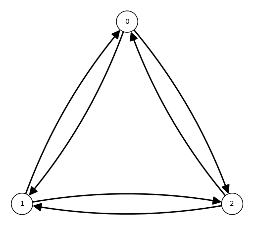
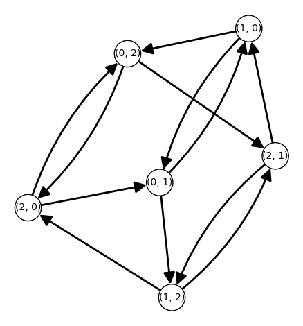
Figure 1: $K_{3}$ and its line digraph

Let $A(\operatorname{LD}(X))$ denote the $(0,1)$-adjacency matrix of $\operatorname{LD}(X)$. Let $R$ denote the arc-reversal matrix, that is, the permutation matrix on the arcs that maps $(a,b)$ to $(b,a)$. We define the transition matrix of the Grover walk on $X$ to be

$$U:=\frac{2}{k}A(\operatorname{LD}(X))-R.$$ (1)

While this definition assumes $X$ is regular, one can in fact define the Grover walk on any graph. Let $C$ be the matrix acting on ${\mathbb{C}}^{\mathrm{arcs}(X)}$, such that for each arc $(u,v)$, its characteristic vector is sent by $C$ to a linear combination of the characteristic vectors of all arcs leaving $u$:

$$Ce_{(u,v)}=\left(\frac{2}{\deg(u)}-1\right)e_{(u,v)}+\frac{2}{\deg(u)}\sum_{w\sim u,\,w\neq v}e_{(u,w)}.$$

This matrix $C$ is unitary and called the coin matrix. Given $R$ and $C$, the alternative definition of the transition matrix is simply $U=RC$ [8]. To see why this definition coincides with (1) when $X$ is regular, we introduce two more matrices, $D_{t}$ and $D_{h}$, whose rows are indexed by the vertices of $X$, and columns by the arcs of $X$:

$$(D_{t})_{u,ab}=\begin{cases}1,\quad u=a\\ 0,\quad\text{otherwise}\end{cases}$$

and

$$(D_{h})_{u,ab}=\begin{cases}1,\quad u=b\\ 0,\quad\text{otherwise}\end{cases}$$

We sometimes refer to $D_{t}$ as the tail-arc incidence matrix, and $D_{h}$ the head-arc incidence matrix. It is not hard to verity the following.

2.1 Lemma.

Let $X$ be a $k$-regular graph. The incidence matrices $D_{t}$ and $D_{h}$ satisfy the following identities.

1. $D_{t}R=D_{h}$

2. $D_{t}D_{t}^{T}=D_{h}D_{h}^{T}=kI$

3. $D_{t}D_{h}^{T}=D_{h}D_{t}^{T}=A(X)$

4. $D_{h}^{T}D_{t}=A(\operatorname{LD}(X))$       

Hence,

$$U =\frac{2}{k}A(\operatorname{LD}(X))-R$$

$$=\frac{2}{k}D_{h}^{T}D_{t}-R$$

$$=R\left(\frac{2}{k}D_{t}^{T}D_{t}-I\right),$$

where $\frac{2}{k}D_{t}^{T}D_{t}-I$ is precisely the coin matrix.

3 Distances in digraphs

Given a digraph $Y$, the distance from $a$ to $b$, denoted $\operatorname{dist}_{Y}(a,b)$, is the length of the shortest dipath in $Y$ from $a$ to $b$. Note that in general $\operatorname{dist}_{Y}(a,b)\neq\operatorname{dist}_{Y}(b,a)$.

There is a simple relation between the distances in a graph and the distances in its line digraph. Recall that for an undirected graph, we view each edge as a pair of opposite arcs.

3.1 Lemma.

Let $X$ be a digraph, and let $(a,b)$ and $(c,d)$ be two arcs of $X$. Then

$$\operatorname{dist}_{\operatorname{LD}(X)}((a,b),(c,d))=\begin{cases}\operatorname{dist}_{X}(c,b)-1,\quad\text{if }(a,b)=(c,d)\\ \operatorname{dist}_{X}(b,c)+1,\quad\text{otherwise}.\end{cases}$$

Proof. The case where $(a,b)$ coincides with $(c,d)$ is trivial. Suppose $(a,b)$ is different from $(c,d)$. If there is a dipath $u_{0}=b,u_{1},u_{2},\cdots,u_{m}=c$ in $X$ from $b$ to $c$, then $(a,u_{0}),(u_{0},u_{1}),(u_{1},u_{2}),\cdots,(u_{m},d)$ is a dipath in $\operatorname{LD}(X)$ from $(a,b)$ to $(c,d)$. This shows

$$\operatorname{dist}_{\operatorname{LD}(X)}((a,b),(c,d))\leq\operatorname{dist}_{X}(b,c)+1$$

Now, suppose $(a,u_{0}),(u_{0},u_{1}),(u_{1},u_{2}),\cdots,(u_{m},d)$ is a shortest dipath in $\operatorname{LD}(X)$ from $(a,b)$ to $(c,d)$. Then for any $i\neq j$, we have $u_{i}\neq u_{j}$, as otherwise we could have removed the portion from $(u_{i},u_{i+1})$ to $(u_{j-1},u_{j})$ to get a shorter dipath. Hence, $u_{0},u_{1},u_{2},\cdots,u_{m}$ is a dipath in $X$ from $b$ to $c$, and so

$$\operatorname{dist}_{X}(b,c)\geq\operatorname{dist}_{LD(X)}((a,b),(c,d))-1.$$

4 Distance regular graphs and their line digraphs

A graph is distance regular if for any two vertices $u$ and $v$ at distance $\ell$, the number of vertices at distance $i$ from $u$ and distance $j$ from $v$ is a constant $p_{ij}^{\ell}$, which depends only on the distances $i$, $j$ and $\ell$. The parameters $p_{ij}^{\ell}$ are called the intersection numbers.

Suppose our graph $X$ is distance regular of diameter $d$. Let $A_{i}=A(X_{i})$ denote the adjacency matrix of its $i$-th distance graph. It is well-known that

$$\{A_{0},A_{1},\ldots,A_{d}\}$$

forms an association scheme (see, for example, [4, Ch 12]). In particular, there are scalars $p_{r}(i)$, called the eigenvalues of the scheme, such that

$$A_{r}=p_{r}(0)A_{0}+p_{r}(1)A_{1}+\cdots+p_{r}(d)A_{d},$$

and scalars $q_{r}(i)$, called the dual eigenvalues of the scheme, such that

$$E_{r}=\frac{1}{|V(X)|}\left(q_{r}(0)A_{0}+q_{r}(1)A_{1}+\cdots+q_{r}(d)A_{d}\right).$$ (2)

Moreover, for any $i$ and $j$, the product $A_{i}A_{j}$ lies in the span of the scheme:

$$A_{i}A_{j}=\sum_{\ell=0}^{d}p_{ij}^{\ell}A_{\ell},$$

and $p_{ij}^{k}$’s are called the intersection numbers.

We can generalize distance regularity to digraphs. A digraph $Y$ is distance regular if for any two vertices $u$ and $v$ with $\operatorname{dist}_{Y}(u,v)=\ell$, the number of vertices $w$ such that $\operatorname{dist}_{Y}(u,w)=i$ and $\operatorname{dist}_{Y}(w,v)=j$ depends only on the distances $i$,$j$ and $\ell$, and we denote this number by $m_{ij}^{\ell}$.

Now, we are ready to show that the line digraph of a distance regular graph is distance regular.

4.1 Lemma.

Let $X$ be a distance regular graph. Let $Y=\operatorname{LD}(X)$ be its line digraph. Then $Y$ is a distance regular digraph. Moreover, for any $i$ and $j$, we have $m_{ij}^{\ell}=m_{ji}^{\ell}$.

Proof. Let $(a,b)$ and $(c,d)$ be two arcs of $X$. We count arcs $(x,y)$ that are at distance $i$ from $(a,b)$ and from which $(c,d)$ is at distance $j$.

We will prove the case where $i,j\geq 1$; the other cases follow from a similar argument. By Lemma 3.1, we are counting elements in the set

$$\Phi:=\{(x,y):\operatorname{dist}_{X}(b,x)=i-1,\operatorname{dist}_{X}(y,c)=j-1,\operatorname{dist}_{X}(x,y)=1\}.$$

On the other hand,

$$(A_{i-1}A_{1}A_{j-1})_{bc}=\sum_{x}\sum_{y}(A_{i-1})_{bx}(A_{1})_{xy}(A_{j-1})_{yc}=\left\lvert\Phi\right\rvert.$$

Since $X$ is distance regular, there are intersection numbers $p_{1,j-1}^{m}$ and $p_{i-1,m}^{\ell}$ such that

$$A_{i-1}A_{1}A_{j-1} =A_{i-1}\sum_{m}p_{1,j-1}^{m}A_{m}$$

$$=\sum_{\ell}\sum_{m}p_{i-1,m}^{\ell}p_{1,j-1}^{m}A_{\ell}.$$

Therefore, the size of $\Phi$ is a constant $m_{ij}^{\ell}$ that depends only on $i$, $j$ and $\ell$. By Lemma 3.1, $\ell$ is determined by the distance from $(a,b)$ to $(c,d)$. Finally, since $A_{i-1}$ commutes with $A_{j-1}$, we have $m_{ij}^{\ell}=m_{ji}^{\ell}$.       

Let $Y$ be a digraph. The $i$-th distance digraph of $Y$, denoted $Y_{i}$, has the same vertex set as $Y$, and vertex $a$ is adjacent to vertex $b$ in $Y_{i}$ if $\operatorname{dist}_{Y}(a,b)=i$. One consequence of Lemma 4.1 is that the $(0,1)$-adjacency matrices of the distance digraphs of $\operatorname{LD}(X)$ commute, if $X$ is distance regular. Moreover, we have a formula for these adjacency matrices.

4.2 Lemma.

Let $X$ be a distance regular graph. Let $A_{i}$ be the adjacency matrix of its $i$-th distance graph. Let $Y=\operatorname{LD}(X)$. Let $Y_{i}$ be the $i$-th distance digraph of $Y$. Then $A(Y_{0})=I$, $A(Y_{2})=D_{h}^{T}A_{1}D_{t}-I$, and for $i=1,3,\cdots,d+1$, $A(Y_{i})=D_{h}^{T}A_{i-1}D_{t}$.

Proof. Clearly, $A(Y_{0})=I$. The remaining statement is a direct translation of Lemma 3.1. Indeed, for $i=1,2\cdots,d$,

$$(D_{h}^{T}A_{i}D_{t})_{(a,b),(c,d)} =e_{(a,b)}^{T}D_{h}^{T}A_{i}D_{t}e_{(c,d)}$$

$$=e_{b}^{T}A_{i}e_{c}$$

$$=\begin{cases}1,\quad\text{if }\operatorname{dist}_{X}(a,b)=i.\\ 0,\quad\mathrm{otherwise}.\end{cases},$$

First assume $i=2,3,\cdots,d+1$. We see that $\operatorname{dist}_{X}(b,c)=i$ if and only if $(a,b)\neq(c,d)$ and

$$\operatorname{dist}_{\operatorname{LD}(X)}((a,b),(c,d))=\operatorname{dist}_{X}(b,c)+1=i+1,$$

from which it follows that $A(Y_{i+1})=D_{h}^{T}A_{i}D_{t}$. Now assume $i=1$. Then $\operatorname{dist}_{X}(b,c)=i$ if and only if $b$ and $c$ are adjacent. If $(a,b)\neq(c,d)$, then

$$\operatorname{dist}_{\operatorname{LD}(X)}((a,b),(c,d))=\operatorname{dist}_{X}(b,c)+1=i+1=2;$$

otherwise,

$$\operatorname{dist}_{\operatorname{LD}(X)}((a,b),(c,d))=\operatorname{dist}_{X}(b,c)-1=i-1=0.$$

Hence $A(Y_{2})+I=D_{h}^{T}A_{1}D_{t}$.       

Using Lemma 4.2, we can verify two properties of $A(Y_{i})$, one of which we have already seen.

4.3 Corollary.

Let $X$ be a distance regular graph. Let $Y=\operatorname{LD}(X)$. Let $Y_{i}$ be the $i$-th distance digraph of $Y$. Then the following statements hold.

1. $A(Y_{0}),A(Y_{1}),\cdots,A(Y_{d+1})$ sum to $J$.

2. $Y$ is distance regular.

Proof. We prove (i); the other statement follows similarly. By Lemma 4.2,

$$\sum_{i=0}^{d+1}A(Y_{i})=I+(D_{h}^{T}A_{0}D_{t})+(D_{h}^{T}A_{1}D_{t}-I)+\sum_{i=2}^{d}D_{h}^{T}A_{i-1}D_{t}$$

which reduces to $D_{h}^{T}JD_{t}$. Since each column of $D_{h}$ or $D_{t}$ has exactly one non-zero entry, we have $D_{h}^{T}JD_{t}=J$.       

Given a digraph $Y$, let $S(Y)$ denote its skew-adjacency matrix, that is,

$$S(Y)=A(Y)-A(Y)^{T}.$$

This represents an oriented graph, that is, a digraph with no symmetric pair of arcs. Note that $A(Y)$ and $A(Y)^{T}$ may not have disjoint supports, so the underlying oriented graph of $S(Y)$ may differ from $Y$. We illustrate this situation in Figure 2.

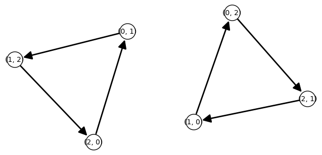
Figure 2: $\operatorname{LD}(K_{3})$ and the underlying oriented graph of $S(\operatorname{LD}(K_{3}))$

Two properties of $S(Y_{i})$ follow from Lemma 4.2 and Corollary 4.3.

4.4 Corollary.

Let $X$ be a $k$-regular distance regular graph. Let $Y_{i}$ be the $i$-th distance digraph of $\operatorname{LD}(X)$. The following statements hold.

1. $S(Y_{1}),S(Y_{2}),\cdots,S(Y_{d+1})$ sum to zero; in particular, they are linearly dependent.

2. For $i,j=1,2,\cdots,d+1$,

   $$S(Y_{i})S(Y_{j})=S(Y_{j})S(Y_{i}).$$

Proof. We have $S(Y_{0})=A(Y_{0})-A(Y_{0})^{T}=0$ and so

$$S(Y_{1})+S(Y_{2})+\cdots+S(Y_{d+1}) =\sum_{i=0}^{d+1}(A(Y_{i})-A(Y_{i})^{T})$$

$$=J-J^{T}$$

$$=0.$$

Also, for $i=1,2,\cdots,d+1$,

$$S(Y_{i})=D_{h}^{T}A_{i-1}D_{t}-D_{t}^{T}A_{i-1}D_{h}.$$

Since

$$A_{i-1}D_{t}D_{h}^{T}A_{j-1} =A_{i-1}D_{h}D_{t}^{T}A_{j-1}=A_{i-1}A_{1}A_{j-1}=A_{j-1}A_{1}A_{i-1},$$

$$A_{i-1}D_{t}D_{t}^{T}A_{j-1} =A_{i-1}D_{h}D_{h}^{T}A_{j-1}=kA_{i-1}A_{1}A_{j-1}=kA_{j-1}A_{1}A_{i-1},$$

it follows that $S(Y_{i})$ commutes with $S(Y_{j})$.       

5 Spectral decomposition

Let $X$ be a $k$-regular distance regular graph of diameter $d$. Recall that the transition matrix $U$ of the Grover walk on $X$ is

$$U=\frac{2}{k}A(\operatorname{LD}(X))-R=R\left(\frac{2}{k}D_{t}^{T}D_{t}-I\right),$$

In this section, we derive some properties of the eigenprojections of $U$.

We first cite a result from [15].

5.1 Theorem.

Every non-real eigenvalue of $U$ comes from an eigenvalue of $A(X)$. More specifically, let $\lambda$ be an eigenvalue of $A(X)$ that is neither $k$ nor $-k$. Let $E_{\lambda}$ be the orthogonal projection onto the $\lambda$-eigenspace of $X$. Suppose $\lambda=k\cos(\theta)$ for some real number $\theta$. Then $e^{i\theta}$ is an eigenvalue of $U$ with eigenprojection

$$F_{\theta_{+}}=\frac{1}{2k\sin^{2}(\theta)}(D_{t}-e^{i\theta}D_{h})^{T}E_{\lambda}(D_{t}-e^{-i\theta}D_{h}),$$

and $e^{-i\theta}$ is an eigenvalue of $U$ with eigenprojection

$$F_{\theta_{-}}=\frac{1}{2k\sin^{2}(\theta)}(D_{t}-e^{-i\theta}D_{h})^{T}E_{\lambda}(D_{t}-e^{i\theta}D_{h}).$$

As a consequence, for any non-real eigenvalue $e^{i\theta}$ of $U$, the difference $F_{\theta_{+}}-F_{\theta_{-}}$ is an imaginary scalar multiple of some real skew-symmetric matrix.

5.2 Corollary.

Let $\lambda$ be an eigenvalue of $A(X)$ that is neither $k$ nor $-k$. Let $E_{\lambda}$ be the orthogonal projection onto the $\lambda$-eigenspace of $X$. Suppose $\lambda=k\cos(\theta)$ for some real number $\theta$. Let $F_{\theta_{+}}$ and $F_{\theta_{-}}$ be the $e^{i\theta}$-eigenprojection and the $e^{-i\theta}$-eigenprojection, respectively. Then

$$F_{\theta_{+}}-F_{\theta_{-}}=\frac{i}{k\sin(\theta)}(D_{t}^{T}E_{\lambda}D_{h}-D_{h}^{T}E_{\lambda}D_{t}).$$

We now fix a $\lambda$ that satisfies the condition in Corollary 5.2, and set

$$S_{\lambda}:=D_{t}^{T}E_{\lambda}D_{h}-D_{h}^{T}E_{\lambda}D_{t}.$$

We show that if $X$ is distance regular, then $S_{\lambda}$ is a linear combination of the skew adjacency matrices of the distance digraphs of $\operatorname{LD}(X)$ , where the coefficients are differences of dual eigenvalues $q_{r}(i)$ defined in Equation (2).

5.3 Lemma.

Let $X$ be a distance regular graph on $n$ vertices of diameter $d$. Let $Y=\operatorname{LD}(X)$. Let $Y_{i}$ be the $i$-th distance digraph of $Y$. If $\lambda$ is the $r$-th eigenvalue of the corresponding association scheme, and $q_{r}(i)$’s are the dual eigenvalues, then

$$S_{\lambda}=\frac{1}{n}\sum_{i=1}^{d}(q_{r}(d)-q_{r}(i-1))S(Y_{i}).$$

Proof. Recall that

$$E_{r}=\frac{1}{n}\left(q_{r}(0)A_{0}+q_{r}(1)A_{1}+\cdots+q_{r}(d)A_{d}\right).$$

If $\lambda$ is the $r$-th eigenvalue in the association scheme, then $E_{\lambda}=E_{r}$ and

$$S_{\lambda} =D_{t}^{T}E_{r}D_{h}-D_{h}^{T}E_{r}D_{t}$$

$$=\frac{1}{n}\sum_{j=0}^{d}q_{r}(j)(D_{t}^{T}A_{j}D_{h}-D_{h}^{T}A_{j}D_{t})$$

$$=-\frac{1}{n}\sum_{j=0}^{d}q_{r}(j)S(Y_{j+1})$$

$$=-\frac{1}{n}\sum_{i=1}^{d+1}q_{r}(i-1)S(Y_{i})$$

$$=\frac{1}{n}\sum_{i=1}^{d}(q_{r}(d)-q_{r}(i-1))S(Y_{i}),$$

where the last equality follows from the fact that $S(Y_{1}),S(Y_{2}),\cdots,S(Y_{d+1})$ sum to zero.       

6 Factoring $U^{2}$

Every unitary matrix $U$ can be written as the exponential of some skew-Hermitian matrix: if

$$U=\sum_{r}e^{i\theta_{r}}F_{r}$$

is the spectral decomposition of $U$, then

$$U=\exp(iH),$$

where $H$ is a Hermitian matrix given by

$$H=\sum_{r}\theta_{r}F_{r}.$$

Now let $X$ be a $k$-regular graph, and $U$ the transition matrix of the Grover walk on $X$. The eigenvalues of $U$ are $\pm 1$ and some complex numbers $e^{\pm i\theta_{r}}$ that come in conjugate pairs. We may assume, without loss of generality, that each $\theta_{r}$ lies in $[0,\pi]$. Then there is a natural way to group the terms in $H$:

$$H=0\cdot F_{0}+\pi\cdot F_{\pi}+\sum_{r:0<\theta_{r}<\pi}\theta_{r}\cdot(F_{r}-{\mkern 2.0mu\overline{\mkern-2.0muF_{r}}}),$$

where $F_{0}$ is the $1$-eigenprojection, $F_{\pi}$ is the $(-1)$-eigenprojection, and $F_{r}$ is the $e^{i\theta_{r}}$-eigenprojection of $U$, respectively.

From Theorem 5.1 and Theorem 5.2 we see that, if $\theta_{r}\in(0,\pi)$, then $k\cos(\theta)$ is an eigenvalue of $A(X)$, and $F_{r}-{\mkern 2.0mu\overline{\mkern-2.0muF_{r}}}$ can be constructed from some eigenspace of $A(X)$. If $-1$ were not an eigenvalue of $U$, then $H$ would take a simpler form

$$H=\sum_{r:0<\theta_{r}<\pi}\theta_{r}(F_{r}-{\mkern 2.0mu\overline{\mkern-2.0muF_{r}}}),$$

which likely bears some combinatorial meaning. Unfortunately, the following result from [15] shows that $-1$ is always an eigenvalue for $U$.

6.1 Lemma.

Let $X$ be a $k$-regular graph on $n$ vertices. Then $(-1)$ is an eigenvalue of $U$, with multiplicity $nk/2-n+2$ if $X$ is bipartite, and $nk/2-n$ otherwise.       

The square of $U$ however may not have $-1$ as an eigenvalue. In fact, if $A(X)$ is invertible, then $\pm i$ are not eigenvalues of $A(X)$, and so $-1$ is not an eigenvalue of $U^{2}$. In this case, we have

$$U^{2}=\exp(iH),$$

where

$$H=2\sum_{r:0<\theta_{r}<\pi}\theta_{r}(F_{r}-{\mkern 2.0mu\overline{\mkern-2.0muF_{r}}}).$$

Our discussion in the last section shows that $H$ is a linear combination of the skew-adjacency matrices of the distance digraphs of $\operatorname{LD}(X)$.

6.2 Theorem.

Let $X$ be a distance regular graph with diameter $d$. Let $U$ be the transition matrix of the Grover walk on $X$. Let $Y_{j}$ be the $j$-th distance digraph of $\operatorname{LD}(X)$. If $A(X)$ is invertible, then there are real scalars $t_{1},t_{2},\ldots,t_{d}$ such that

$$U^{2}=\exp(t_{1}S(Y_{1}))\exp(t_{1}S(Y_{2}))\cdots\exp(t_{d}S(Y_{d})).$$

Moreover, if $n$ is the number of vertices in $X$, and $p_{r}(j)$’s and $q_{r}(j)$’s are the eigenvalues and dual eigenvalues of the association scheme, then

$$t_{j}=\frac{2}{n}\sum_{r:-k<p_{1}(r)<k}\frac{\arccos(p_{1}(r)/k)}{\sqrt{k^{2}-(p_{1}(r))^{2}}}(q_{r}(j-1)-q_{r}(d)).$$

Proof. We have

$$U^{2}=\exp(iH)$$

where

$$H=2\sum_{r:0<\theta_{r}<\pi}\theta_{r}(F_{r}-{\mkern 2.0mu\overline{\mkern-2.0muF_{r}}}).$$

By Lemma 5.3, for each eigenvalue $p_{1}(r)\in(-k,k)$,

$$S_{p_{1}(r)}=\frac{1}{n}\sum_{j=1}^{d}(q_{r}(d)-q_{r}(j-1))S(Y_{j}),$$

and so by Corollary 5.2,

$$H =2i\sum_{r:-k<p_{1}(r)<k}\frac{\arccos(p_{1}(r)/k)}{\sqrt{k^{2}-(p_{1}(r))^{2}}}(D_{t}^{T}E_{p_{1}(r)}D_{h}-D_{h}^{T}E_{p_{1}(r)}D_{t})$$

$$=\frac{2i}{n}\sum_{r:-k<p_{1}(r)<k}\frac{\arccos(p_{1}(r)/k)}{\sqrt{k^{2}-(p_{1}(r))^{2}}}\sum_{j=1}^{d}(q_{r}(d)-q_{r}(j-1))S(Y_{j}).$$

Finally, by Corollary 4.4, these skew-adjacency matrices $S(Y_{j})$ commute, so we can factor $U^{2}$ into the desired form.       

If we rewrite $\exp(t_{i}S(Y))$ in the above theorem as $\exp(it_{i}(iS(Y_{i})))$, then we have the transition matrix of a continuous-time quantum walk on an oriented graph, evaluated at time $t_{i}$. Thus, for a distance regular graph with diameter $d$ and invertible adjacency matrix, the Grover walk on it factors into at most $d$ continuous-time quantum walks on the distance digraphs of $\operatorname{LD}(X)$. In particular, a discrete-time quantum walk on $K_{n}$ is equivalent to a continuous-time quantum walk on its line digraph.

6.3 Corollary.

Let $U$ be the Grover walk on $K_{n}$. Then

$$U^{2}=\exp(tS(\operatorname{LD}(K_{n})))$$

where

$$t=\frac{2\arccos(1/(1-n))}{\sqrt{n^{2}-2n}}.$$

Proof. The association scheme for $K_{n}$ is

$$\{A_{0}=I,\quad A_{1}=J-I\},$$

with eigenprojections

$$E_{0}=\frac{1}{n}J,\quad E_{1}=I-\frac{1}{n}J,$$

eigenvalues

$$p_{0}(0)=p_{0}(1)=1,\quad p_{1}(0)=n-1,\quad p_{1}(1)=-1,$$

and dual eigenvalues

$$q_{1}(0)=q_{0}(1)=1,\quad q_{1}(0)=n-1,\quad q_{1}(1)=-1.$$

The result then follows from a direct calculation.       

The Grover walk on an invertible strongly regular graph factors into at most two continuous-time quantum walks. For the Petersen graph $P$, the factors of $U^{2}$ are continuous-time quantum walks on the oriented graphs shown in Figure 3.

Figure 3: Underlying oriented graphs of $S(\operatorname{LD}(P))$ and $S(\operatorname{LD}(P)_{2})$

Finally, we remark here that not all $d$ distance digraphs may show up in the factorization. For example, if $U$ is the Grover walk of the $3$-cube $Q_{3}$, and $Y_{2}$ is the second distance digraph of $\operatorname{LD}(Q_{3})$, then there is a scalar $t$ such that $U^{2}=\exp(tS(Y_{2}))$. It will be interesting to characterize distance regular graphs on which the discrete-time quantum walk factors into fewer than $d$ continuous-time quantum walks.

7 Implementing the search algorithm

We show how the aforementioned factorization allows us to implement some search algorithms using continuous-time quantum walks. To start, we introduce a quantum walk based search algorithm due to Shenvi, Kempe and Whaley [11]. Given a graph $X$ and a marked vertex $a$, the oracle, denoted $O_{a}$, is the diagonal matrix indexed by the arcs of $X$, such that

$$(O_{a})_{(u,v),(u,v)}=\begin{cases}-1,&\quad u=a,\\ 1,&\quad u\neq 1.\end{cases}$$

Assume $X$ is $k$-regular on $n$ vertices. The state space associated with $X$ is ${\mathbb{C}}^{n}\otimes{\mathbb{C}}^{k}$, the vector space of complex-valued functions on the arcs, and the oracle $O_{a}$ can be written as

$$O_{a}=(I-2E_{aa})\otimes I.$$

To find the marked vertex $a$, we apply the oracle $O_{a}$ and the transition matrix $U$ of the Grover walk alternately to the following initial state:

$$x_{0}=\frac{1}{\sqrt{nk}}{\bf 1}_{n}\otimes{\bf 1}_{k}.$$

Thus, at time $t$, the system is in state

$$x_{t}=(UO_{a})^{t}x_{0}.$$

If we measure at time $t$, the outcome will be an arc $(u,v)$ with probability

$$\left\lvert\langle x_{t},e_{(u,v)}\rangle\right\rvert^{2}.$$

We call the sum

$$\sum_{v\sim a}\left\lvert\langle x_{t},e_{(a,v)}\rangle\right\rvert^{2}$$

the success probability of finding the marked vertex at time $t$.

The well-known Grover’s search algorithm [7] is equivalent to finding a marked vertex using the above procedure - the underlying graph is a complete graph $K_{n}$ with a loop at each vertex, and the success probability is reasonably high at time $t=O(\sqrt{n})$.

While one walk step per oracle query seems standard in search algorithms, Wong and Ambainis [13] proposed a modification, where the algorithm takes multiple walk steps per oracle query. That is, the transition matrix in this algorithm is

$$U^{k}O_{a}$$

for some positive integer $k$. Thus, if $k$ is even and $X$ is an invertible distance regular graph, we can implement the walk steps $U^{k}$ using continuous-time quantum walks. As for the oracle query, note that $O_{a}$ has spectral decomposition

$$O_{a}=1\cdot((I-E_{aa})\otimes I)+(-1)\cdot(E_{aa}\otimes I),$$

and so

$$O_{a}=\exp(i\pi(E_{aa}\otimes I)).$$

The underlying graph of $E_{aa}\otimes I$ consists of isolated vertices, each representing an arc of $X$, and every vertex representing an outgoing arc of $a$ has a loop on it. Thus, we can implement $O_{a}$ by running a continuous-time quantum walk on this graph for the time period of $\pi$.

8 Generalization to association schemes, and future work

We have seen that for an invertible distance regular graph $X$, a discrete-time quantum walk on $X$ factors into continuous-time quantum walks on the distance digraphs of the line digraph of $X$. It will be interesting to translate properties on the discrete side, such as perfect state transfer, into properties on the continuous side, and vice versa.

In general, if the adjacency matrix of a graph $X$ is invertible and lies in the Bose Mesner algebra of some association scheme, then we have a similar factorization.

8.1 Theorem.

Let ${\mathcal{A}}=\{A_{0},A_{1},\ldots,A_{d}\}$ be an association scheme. Let $D_{t}$ and $D_{h}$ be the arc-tail and arc-head incidence matrices of $X_{1}$. For each $i=0,1,\cdots,d$, define a skew-symmetric $(1,-1)$-matrix by

$$S_{i}=D_{h}^{T}A_{i}D_{t}-D_{t}^{T}A_{i}D_{h}.$$

Then $S_{i}S_{j}=S_{j}S_{i}$.

Let $X$ be a graph whose adjacency is invertible and lies in the Bose Mesner algebra of ${\mathcal{A}}$. Let $U$ be the transition matrix of the Grover walk on $X$. Then there are real scalars $t_{1},t_{2},\ldots,t_{d}$ such that

$$U^{2}=\exp(t_{1}S_{1})\exp(t_{2}S_{2})\cdots\exp(t_{d}S_{d}).$$

Proof. The fact that $S_{i}$ commutes with $S_{j}$ follows from Lemma 2.1 and that $A_{0},A_{1},\ldots,A_{d}$ commute with each other.

For the second part, note that the Bose Mesner algebra of ${\mathcal{A}}$ has a basis $\{E_{0},E_{1},\ldots,E_{d}\}$ of idempotents. By the spectral decomposition of $U$ and Corollary 5.2, we see that $U^{2}=\exp(iH)$, where $H$ lies in

$$\mathrm{span}\{D_{t}^{T}E_{i}D_{h}-D_{h}^{T}E_{i}D_{t}:i=0,1,\cdots,d\},$$

that is,

$$\mathrm{span}\{D_{t}^{T}A_{i}D_{h}-D_{h}^{T}A_{i}D_{t}:i=0,1,\cdots,d\}.$$

When $X$ is distance regular, the matrix $S_{i}$ in the above theorem has a nice interpretation: it is the skew-adjacency matrix of the $i$-th distance digraph of the line digraph of $X$. In the more general situation, however, the relation between $S_{i}$ and $X$ has not been explored. It will be helpful to look into a few common association schemes, such as groups schemes, and study the “lift” of the Schur idempotents via the the arc-tail and arc-head incidence matrices.

9 Acknowledgment

The author would like to thank Ada Chan for her inspiring discussion, and David Roberson for bringing up the generalization to association schemes. The author acknowledges the support of the York Science Fellow program. The author thanks the anonymous referees for their valuable comments.

References

• [1] Dorit Aharonov, Andris Ambainis, Julia Kempe, and Umesh Vazirani, Quantum walks on graphs, Proceedings of the 33rd Annual ACM Symposium on Theory of Computing (2001), 50–59.
• [2] Ada Chan, Complex Hadamard matrices, instantaneous uniform mixing and cubes, Algebraic Combinatorics 3 (2020), no.Β 3, 757–774.
• [3] Ada Chan, Gabriel Coutinho, Christino Tamon, Luc Vinet, and Hanmeng Zhan, Quantum fractional revival on graphs, Discrete Applied Mathematics 269 (2019), 86–98.
• [4] Chris Godsil, Algebraic combinatorics, Chapman & Hall, 1993.
• [5]  , When can perfect state transfer occur?, Electronic Journal of Linear Algebra 23 (2012), no.Β 1, 877–890.
• [6] Chris Godsil and Krystal Guo, Quantum walks on regular graphs and eigenvalues, Electronic Journal of Combinatorics 18 (2011), Paper 165.
• [7] Lov Grover, A fast quantum mechanical algorithm for estimating the median, Proceedings of the 28th Annual ACM Symposium on the Theory of Computing (1996), 212–219.
• [8] Viv Kendon, Quantum walks on general graphs, International Journal of Quantum Information (2006), 791–805.
• [9] Norio Konno, Iwao Sato, and Etsuo Segawa, Phase measurement of quantum walks: Application to structure theorem of the positive support of the Grover walk, Electronic Journal of Combinatorics 26 (2019), no.Β 2, P2.26.
• [10] R.Β Portugal, R.Β Santos, T.Β Fernandes, and D.Β GonΓ§alves, The staggered quantum walk model, Quantum Information Processing 15 (2016), no.Β 1, 85–101.
• [11] Neil Shenvi, Julia Kempe, and KΒ Whaley, Quantum random-walk search algorithm, Physical Review A 67 (2003), no.Β 5, 52307.
• [12] Mario Szegedy, Quantum speed-up of Markov chain based algorithms, 45th Annual IEEE Symposium on Foundations of Computer Science (2004), 32–41.
• [13] ThomasΒ G. Wong and Andris Ambainis, Quantum search with multiple walk steps per oracle query, Physical Review A - Atomic, Molecular, and Optical Physics 92 (2015), no.Β 2, 022338.
• [14] Yusuke Yoshie, Periodicities of Grover Walks on Distance-Regular Graphs, Graphs and Combinatorics 35 (2019), no.Β 6, 1305–1321.
• [15] Hanmeng Zhan, An infinite family of circulant graphs with perfect state transfer in discrete quantum walks, Quantum Information Processing 18 (2019), no.Β 12, 1–26.