IIB matrix model: Extracting the spacetime points

Abstract

Assuming that the large-$N$ master field of the Lorentzian IIB matrix model has been obtained, we go through the procedure of how the coordinates of emerging spacetime points can be extracted. Explicit calculations with test master fields suggest that the genuine IIB-matrix-model master field may have a fine-structure that is essential for producing the spacetime points of an expanding universe.

I Introduction

The IIB matrix model IKKT-1997 ; Aoki-etal-review-1999 has been studied numerically in its Lorentzian version KimNishimuraTsuchiya2012 ; NishimuraTsuchiya2019 ; Hatakeyama-etal2020 . But how, conceptually, a classical spacetime emerges in Refs. IKKT-1997 ; Aoki-etal-review-1999 ; KimNishimuraTsuchiya2012 ; NishimuraTsuchiya2019 ; Hatakeyama-etal2020 was unclear.

It has been suggested, in App. B of the preprint version Klinkhamer2019-emergence-v6 of Ref. Klinkhamer2019-emergence-PTEP , that the large-$N$ master field must play a crucial role for the emergence of a classical spacetime. As a follow-up, Ref. Klinkhamer2020 presented an explicit (coarse-graining) procedure for extracting classical spacetime from the master field.

Here, we give some numerical results to illustrate the procedure of Ref. Klinkhamer2020 , as regards the extraction of the spacetime points (the extraction of a spacetime metric is more difficult and will not be discussed here). First, we consider a test master field with randomized entries on a band diagonal and, then, we consider a specially designed test master field with a deterministic fine-structure, which gives rise to multiple strands of spacetime that appear to fill out an expanding universe. This last type of test master field provides an existence proof that there can be master fields for which the procedure of Ref. Klinkhamer2020 produces more or less acceptable spacetime points.

II Test master fields

The discussion of the temporal test matrix is relatively simple, as the master field $\underline{\widehat{A}}^{\;0}$ is assumed to have been diagonalized and ordered by an appropriate global gauge transformation Klinkhamer2020 . This $N\times N$ traceless Hermitian test matrix is obtained as follows:

$$\underline{\widehat{A}}^{\;0}_{\text{\,test}} = \text{diag}\,\Big{[}\overline{\alpha}(1),\,\ldots\,,\,\overline{\alpha}(N)\Big{]}\,,$$ (1a)

$$\overline{\alpha}(i) = \widetilde{\alpha}(i)-\frac{1}{N}\;\left(\sum_{j=1}^{N}\widetilde{\alpha}(j)\right)\,,$$ (1b)

$$\widetilde{\alpha}(i) = \text{rand}\left[\frac{i-1}{N},\,\frac{i}{N}\right]\,,$$ (1c)

with $i\in\{1,\,\ldots,\,N\}$ and $\text{rand}\big{[}x,\,y\big{]}$ giving a uniform pseudorandom real number in the interval $[x,\,y]$.

Next, we construct a test master field $\underline{\widehat{A}}^{\;1}_{\text{\,test-1}}$ with a band-diagonal structure of width $\Delta N$ and average absolute values along the diagonal given by a parabola with approximate value $1$ halfway ($i\sim N/2$) and approximate value $2$ at the edges ($i=1$ and $i=N$). Specifically, this $N\times N$ traceless Hermitian matrix with bandwidth $\Delta N$ (assumed to be even) is obtained as follows:

$$\underline{\widehat{A}}^{\;1}_{\text{\,test-1}} = \frac{1}{2}\;\left(\overline{A}^{\;1}+\overline{A}^{\,1\;\dagger}\right)-\frac{1}{N}\;\text{tr}\,\left[\frac{1}{2}\;\left(\overline{A}^{\;1}+\overline{A}^{\,1\;\dagger}\right)\right]\,\makebox[2.58334pt][l]{$1$}{\rm l}_{\,N}\,,$$ (2a)

$$\left(\overline{A}^{\;1}\right)_{i,\,j} = \begin{cases}r_{\chi}\;\overline{x}^{\;1}(i)\,,&\text{for}\;j-\Delta N/2\leq i\leq j+\Delta N/2\,,\\[5.69054pt] 0\,,&\text{otherwise}\,,\end{cases}\,,$$ (2b)

$$r_{\chi} = (1-\chi)\;\text{rand}\big{[}-2,\,+2\big{]}+\chi\;\text{rand}\big{[}\pm 1\big{]}\,,$$ (2c)

$$\overline{x}^{\;1}(i) = 1+\left[\left(i-\frac{1}{2}\right)\frac{2}{N}-1\right]^{2}\,,$$ (2d)

$$\chi \in \{0,\,1\}\,,$$ (2e)

with $\makebox[2.58334pt][l]{$1$}{\rm l}_{\,N}$ the $N\times N$ identity matrix, indices $i$ and $j$ taking values in $\{1,\,\ldots,\,N\}$, $\text{rand}\big{[}x,\,y\big{]}$ defined below (1c), and $\text{rand}\big{[}\pm 1\big{]}$ giving $+1$ with probability $1/2$ and $-1$ with probability $1/2$.. The parameter $\chi$ distinguishes between a continuous or a discrete range for the randomized entries on the individual rows of the band diagonal of the matrix. The “expanding” behavior (2d), with a minimum at the halfway point, mimics the numerical results obtained in Refs. KimNishimuraTsuchiya2012 ; NishimuraTsuchiya2019 ; Hatakeyama-etal2020 , assuming that $\overline{x}^{\;1}$ corresponds to one of the “large” dimensions of the $3+6$ split. The numerical results of these last references may, in fact, give a rough approximation of the genuine IIB-matrix-model master field (especially interesting are the $N=128$ and $N=192$ matrices obtained in Ref. NishimuraTsuchiya2019 ).

The analysis in the sections below will start from the test-1 master field (1) and (2), but, later, will also consider a test-2 master field $\underline{\widehat{A}}^{\;1}_{\text{\,test-2}}$ with more structure. Roughly speaking, this test-2 master field again has a band-diagonal structure with parabolic behavior, but now there is also a finer modulation of $(2\,\Delta N)\times(2\,\Delta N)$ diagonal blocks, which alternatingly are reduced by a positive factor $\kappa<1$ or boosted by a positive factor $\lambda>1$, and a further modulation of $\Delta N\times\Delta N$ diagonal blocks, which alternatingly have $+1$ or $-1$ on the diagonal.

Assuming $N$, $\Delta N$, and $N/\Delta N\equiv L$ all to be even integers, this $N\times N$ traceless Hermitian test matrix is given by the following expression:

$$\underline{\widehat{A}}^{\;1}_{\text{\,test-2}} = \frac{1}{2}\;\left(\widetilde{A}^{\;1}+\widetilde{A}^{\,1\;\dagger}\right)-\frac{1}{N}\;\text{tr}\,\left[\frac{1}{2}\;\left(\widetilde{A}^{\;1}+\widetilde{A}^{\,1\;\dagger}\right)\right]\,\makebox[2.58334pt][l]{$1$}{\rm l}_{\,N}\,,$$ (3a)

$$\widetilde{A}^{\;1} = D_{\kappa\lambda}\cdot D_{\text{pm}}\cdot\overline{A}^{\;1}\,,$$ (3b)

$$D_{\kappa\lambda} = \text{diag}\big{[}\kappa,\,\ldots\,,\,\kappa,\,\lambda,\,\ldots\,,\,\lambda,\,\,\ldots\,,\,\lambda,\,\ldots\,,\,\lambda\big{]}\,,$$ (3c)

$$D_{\text{pm}} = \text{diag}\big{[}+1,\,\ldots\,,\,+1,\,-1,\,\ldots\,,\,-1,\,\,\ldots\,,\,-1,\,\ldots\,,\,-1\big{]}\,,$$ (3d)

$$\left(\overline{A}^{\;1}\right)_{i,\,j} = \begin{cases}\overline{r}_{\xi}\,\overline{x}^{\;1}(i)\,,&\text{for}\;j-\Delta N/2\leq i\leq j+\Delta N/2\,,\\[5.69054pt] 0\,,&\text{otherwise}\,,\end{cases}\,,$$ (3e)

$$\overline{r}_{\xi} = \text{rand}\big{[}1-\xi,\,1+\xi\big{]}\,,$$ (3f)

$$\overline{x}^{\;1}(i) = 1+\left[\left(i-\frac{1}{2}\right)\frac{2}{N}-1\right]^{2}\,,$$ (3g)

$$0 < \kappa\leq 1\leq\lambda\,,$$ (3h)

$$0 < \xi<1\,,$$ (3i)

with $i,\,j\in\{1,\,\ldots,\,N\}$ and $\text{rand}\big{[}x,\,y\big{]}$ defined below (1c). The real numbers $\kappa$ and $\lambda$ in (3c) are each repeated $2\,\Delta N$ times [making for $L/2$ diagonal $(2\,\Delta N)\times(2\,\Delta N)$ blocks] and the real numbers $+1$ and $-1$ in (3d) are each repeated $\Delta N$ times [making for $L$ diagonal $\Delta N\times\Delta N$ blocks].

The $\pm 1$ fine-structure of (3d) is inspired by the similar fine-structure of an exact “classical” solution with $\Delta N\sim 1$ found in App. A of Ref. Klinkhamer2019-emergence-PTEP . The raison d’$\,\hat{\text{e}}$tre of the $\kappa,\,\lambda$ fine-structure in (3c) will become clear in Sec. V. Remark also that the IIB-matrix-model variables are complex Hermitian, whereas the two test master fields of this section are real.

III Extraction procedure

The procedure for obtaining spacetime points from the master field has been outlined in Sec. IV of Ref. Klinkhamer2020 . The basic idea is to consider, in each of the ten matrices $\underline{\widehat{A}}^{\,\mu}$, the $K$ blocks of size $n\times n$ centered on the diagonal. Here, we assume that $N=K*n$, for positive integers $K$ and $n$, and that $\underline{\widehat{A}}^{\,0}$ has already been diagonalized and ordered by an appropriate global gauge transformation. The coordinates of the spacetime points are then obtained from the average of the eigenvalues in each $n\times n$ block. If the IIB-matrix-model master field $\underline{\widehat{A}}^{\,\mu}$ has a diagonal band width $\Delta N$, we expect that $n$ must be chosen to be approximately equal to $\Delta N$ or, better, significantly larger than $\Delta N$. Furthermore, it is possible to introduce a length scale $\ell$ into the IIB matrix model, as discussed in Ref. Klinkhamer2020 , so that the bosonic matrix variable $A^{\mu}$ carries the dimension of length, as does the corresponding master field $\underline{\widehat{A}}^{\,\mu}$. Throughout this article, we take length units which set $\ell=1$.

The test master field $\underline{\widehat{A}}^{\;0}_{\text{\,test}}$, as given by (1), then gives the following temporal coordinate:

$$\widehat{x}^{\;0}(\sigma)\equiv\widetilde{c}\;\widehat{t}(\sigma)=\frac{1}{n}\;\sum_{l=1}^{n}\,\overline{\alpha}_{(k-1)\,n+l}\,,$$ (4)

for $\sigma\equiv k/K\in(0,\,1]$ with $k\in\{1,\,\ldots,\,K\}$ and $K=N/n$. The velocity $\widetilde{c}$ in (4) will be set to unity in the following. The temporal coordinate $\widehat{t}^{\;1}(\sigma)$ takes values in the range $[-0.5,\,0.5]$.

Similarly, the test-1 master field $\underline{\widehat{A}}^{\;1}_{\text{\,test-1}}$, as given by (2), gives the following coordinate in one spatial dimension:

$$\widehat{x}^{\;1}(\sigma)=\frac{1}{n}\;\sum_{l=1}^{n}\,\left[\,\overline{\beta}^{\;1}\right]_{(k-1)\,n+l}\,,$$ (5)

for $\sigma\equiv k/K\in(0,\,1]$ and eigenvalues $\overline{\beta}^{\;1}_{i}$ of the $n\times n$ blocks along the diagonal in the $N\times N$ matrix (2). The same expression (5) gives a spatial coordinate from the test-2 master field (3).

Before we start with the explicit calculation of the spacetime points (4) and (5) from our test master fields, we have a few general remarks on the adopted coarse-graining procedure. In order to cover the $\Delta N$ band diagonal of the master field completely, it would perhaps be better to let the $n\times n$ blocks, with $n>\Delta N$, overlap halfway. But, then, there would be the problem of double-counting some of the information contained in the master field and, moreover, there would be no way to obtain a clear ordering of the extracted information with respect to time. For these reasons, we prefer to keep, in our exploratory analysis, the simple procedure of having the $n\times n$ blocks touch on the diagonal, without overlap: even though the $n\times n$ block eigenvalues are not perfect (some information from the master field has been lost), there is a clear ordering of the average (5) with respect to the coordinate time $t$ from (4).

IV Spacetime points from the test-1 master field

Now, choose fixed values of $N$ (assumed to be odd) and $\Delta N$ (assumed to be even) in the test master field $\widehat{A}^{\;1}_{\text{\,test-1}}$ from (2) for $\chi=0$. Then, for various choices of the block size $n$ (which must be odd, because $N$ has been assumed to be odd), the procedure from Sec. III gives the spatial coordinate $\widehat{x}^{\;1}(\sigma)$ from (5), for $\sigma\in(0,\,1]$. Numerical results are presented in the upper panel-quartet of Fig. 1. All numerical results reported in this paper were obtained with Mathematica 5.0 Wolfram1991 . See, in particular, Sec. 3.2.3 of Ref. Wolfram1991 for the use of pseudorandom numbers in Mathematica and Chap. 3 of Ref. Knuth1998 for a general discussion.

The calculation of the temporal coordinate is simpler, as the test master field $\underline{\widehat{A}}^{\;0}_{\text{\,test}}$ from (1) is already diagonal with explicit eigenvalues. The temporal coordinate $\widehat{t}(\sigma)$ follows from (4) for $\widetilde{c}=1$ and $\sigma\in(0,\,1]$. It turns out that $\widehat{t}$ is approximately linearly proportional to $\sigma$, as shown by the lower panel-quartet of Fig. 1. From these results we obtain $\widehat{x}^{\;1}\big{(}\,\widehat{t}\>\big{)}$, as shown by Fig. 3.

For completeness, we also show, in Fig. 3, the results with discrete values ($\chi=1$) on the rows of the band diagonal for $\Delta N=4$, where the role of the $\chi$ parameter has been explained in the sentence starting below (2e). Similar $n=3$ results have been obtained for $\Delta N=2$ and $\Delta N=6$.

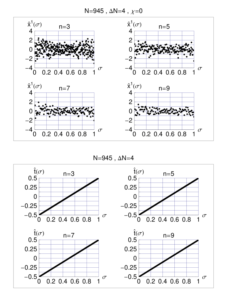
Figure 1: The spatial coordinate $\widehat{x}^{\;1}(\sigma)$, for $\sigma\in(0,\,1]$, is shown in the upper panel-quartet. This coordinate $\widehat{x}^{\;1}(\sigma)$ is obtained by the procedure of Sec. III applied to the test-1 master field $\widehat{A}^{\;1}_{\text{\,test-1}}$ as given by (2), for matrix size $N=3*5*7*9=945$, band-diagonal width $\Delta N=4$, and parameter $\chi=0$ to select a continuous range of values on the individual rows of the band diagonal of the matrix. The temporal coordinate $\widehat{t}^{\;1}(\sigma)$, obtained by applying the same procedure to the matrix (1), is shown in the lower panel-quartet. Eliminating $\sigma$ between $\widehat{x}^{\;1}(\sigma)$ and $\widehat{t}(\sigma)$ gives $\widehat{x}^{\;1}\big{(}\,\widehat{t}\>\big{)}$, which is shown in Fig. 3.

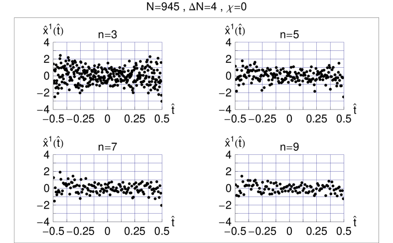
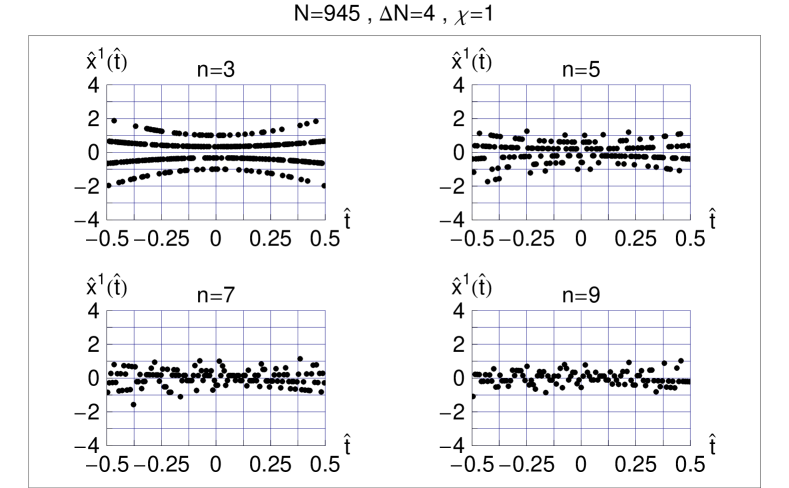
Figure 2: Behavior of $\widehat{x}^{\;1}$ versus $\widehat{t}$ from the test-1 results of Fig. 1.

Figure 3: Same as Fig. 3, but the test-1 master field (2) now has parameter $\chi=1$ to select a discrete range of values on the individual rows of the band diagonal of the matrix.

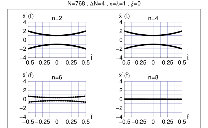
Figure 4: Behavior of $\widehat{x}^{\;1}$ versus $\widehat{t}\,$ from the test-2 master field (3), for $N=2^{8}*3=768$ and $\Delta N=4$, and with trivial modulation parameters, $\kappa=\lambda=1$, and vanishing randomization parameter, $\xi=0$.

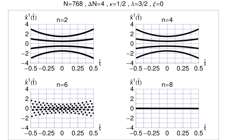
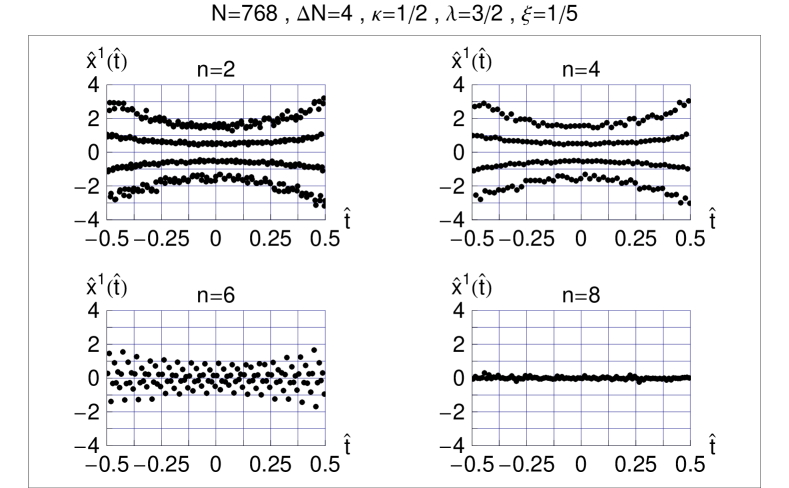
Figure 5: Same as Fig. 4, but now with nontrivial modulation parameters, $\kappa=1/2$ and $\lambda=3/2$.

Figure 6: Same as Fig. 6, but now with a nonvanishing randomization parameter, $\xi=0.2$.

V Spacetime points from the test-2 master field

The $n=3$ results of Fig. 3 perhaps show a point set expanding with time $|t|$, but it is not clear if a classical spacetime emerges with an expanding volume (at this moment, we do not have the metric distance between the points). In that sense, the $n=3$ results of Fig. 3 may be more promising, as they suggest four “strands” of spacetime separating from each other as $|t|$ increases (we are using “strand” in the meaning of a “strand of pearls”). Incidentally, a somewhat related pattern has been observed in Fig. 5 of Ref. Hatakeyama-etal2020 .

Returning to the strands of Fig. 3, the following question arises: is it at all possible to design a special master field $\underline{\widehat{A}}^{\;1}_{\text{\,special}}$, so that the procedure of Sec. III gives multiple strands of spacetime, which fill out an expanding universe?

The answer is affirmative and an example for up to four spacetime strands is given by the test-2 matrix (3). For $\kappa=\lambda=1$, we get two strands (Fig. 4) and, for $\kappa=1/2$ and $\lambda=3/2$, for example, we get four strands with $n=2$ and $n=4$ averaging (Figs. 6 and 6); the $n=6$ results of Fig. 6 even suggest the presence of six strands. It appears possible to get more than four (or six) spacetime strands by introducing even more parameters and structure along the diagonal of the test matrix.

The main open problem, now, is to obtain the emergent metric and to calculate the metric distances between points on a single strand and between points on different strands. At this moment, we have no solid results but only some speculative remarks. One speculative remark is that, for two strands extending in two “large” spatial dimensions, two “neighboring” points on a single strand may have a smaller metric distance than two “neighboring” points on different adjacent strands. Appendix A reports on a toy-model calculation which suggests such a result.

VI Discussion

In this somewhat technical paper, we have considered several test matrices and obtained tentative spacetime points by applying the procedure of Ref. Klinkhamer2020 to these matrices (an alternative procedure is presented in App. B). These test matrices have a band-diagonal structure, one being strictly diagonal to represent the time coordinate $t$ and another having a finite bandwidth $\Delta N$ to represent a typical spatial coordinate $x^{1}$ from a “large” dimension, whose average absolute value $|x^{1}|$ grows quadratically with $t$ (a behavior seen in the numerical results of Refs. KimNishimuraTsuchiya2012 ; NishimuraTsuchiya2019 ; Hatakeyama-etal2020 ). The hope is that these test matrices may help us to understand a possible fine-structure of the genuine IIB-matrix-model master field.

As a first step towards such an understanding, we have constructed the test-2 matrix from (3), which has a very special fine-structure to allow for the appearance of multiple “strands” of spacetime (Figs. 4–6). In fact, this understanding allows us to interpret the somewhat surprising $n=3$ and $n=5$ results of Fig. 3, which indicate the appearance of, respectively, four and six strands (with some good will, the $n=7$ results can be seen to hint at the presence of eight strands). The heuristic idea, now, is that the simple flip-flop behavior on each row of the matrix gives a repeating pattern if a sufficiently large number of rows is considered ($N\to\infty$). Preliminary numerical results extending the calculation of Fig. 3 appear to confirm the appearance of more than six strands.

Many questions remain as to the procedure for the extraction of the spacetime points, not to mention the spacetime metric. But even more important, at this moment, is to obtain a reliable approximation of the IIB-matrix-model master field, which may or may not display some form of fine-structure.

Appendix A Toy-model calculation of metric distances

In this appendix, we report on a toy-model calculation which extends a similar calculation presented in App. B of Ref. Klinkhamer2020 .

Start from the emergent inverse metric as given by (5.1) of Ref. Klinkhamer2020 (based on an earlier expression from Ref. Aoki-etal-review-1999 ):

$$g^{\mu\nu}(x)\sim\int_{\mathbb{R}^{10}}d^{10}y\;\langle\langle\,\rho(y)\,\rangle\rangle\;(x-y)^{\mu}\,(x-y)^{\nu}\;f(x-y)\;r(x,\,y)\,,$$ (6)

where $\langle\langle\,\rho(x)\,\rangle\rangle$ is the average density function of emergent spacetime points, $r(x,\,y)$ is the correlation function from these density functions, and $f(x-y)$ is a correlation function that appears in the effective action of a low-energy scalar degree of freedom; see Refs. Aoki-etal-review-1999 ; Klinkhamer2020 for further details.

Restrict (6) to two “large” spatial dimensions (with coordinates $x^{2}$ and $x^{3}$) and consider a simple setup in the $(x^{2},\,x^{3})$ plane with two finite bands $B_{+}$ and $B_{-}$ (Fig. 7),

$$B_{+} = \big{\{}(x^{2},\,x^{3})\,\big{|}\,x^{2}\in[-2,\,2]\;,\;x^{3}\in[+1-\Delta x/2,\,+1+\Delta x/2]\big{\}}\,,$$ (7a)

$$B_{-} = \big{\{}(x^{2},\,x^{3})\,\big{|}\,x^{2}\in[-2,\,2]\;,\;x^{3}\in[-1-\Delta x/2,\,-1+\Delta x/2]\big{\}}\,,$$ (7b)

$$0 < \Delta x/2<1\,,$$ (7c)

where the bands may be thought to arise from wiggly strands such as shown by the $n=4$ results of Fig. 6. The average density of emerging spacetime points is assumed to be nonvanishing only over these bands,

$$\langle\langle\,\rho(x)\,\rangle\rangle=\begin{cases}1/\ell^{10}\,,&\text{for}\;(x^{2},\,x^{3})\in B_{+}\cup B_{-}\,,\\[5.69054pt] 0\,,&\text{otherwise}\,,\end{cases}\,,$$ (8)

with $\ell$ the length scale of the IIB matrix model and all coordinates $x^{\mu}$ carrying the dimension of length, as discussed in Sec. III. The length units of the setup in Fig. 7 are assumed to correspond to $\ell=1$.

Next, introduce a symmetric cutoff on the integrals at $\pm 2$ and make two further simplifications,

$$f(x) = 1/\ell^{2}\,,$$ (9a)

$$r(x,\,y) = 1\,,$$ (9b)

with $\ell=1$ for the chosen length units. Note that the assumptions (9) perhaps make sense if the space patch considered is sufficiently small in physical units; see also the discussion below for another setup.

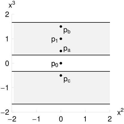
Figure 7: Setup for the toy-model calculation, where the shaded areas indicate the bands $B_{\pm}$ (centered on $x^{3}=\pm 1$ and having widths $\Delta x=4/3$) over which spacetime points emerge. Metric components at two points $p_{0}$ and $p_{1}$ are compared and metric distances between three further points $p_{a}$, $p_{b}$, and $p_{c}$ calculated.

It is, now, straightforward to calculate the inverse metric components $g^{22}$, $g^{33}$, and $g^{23}=g^{32}$ from (6) for two points $p_{0}$ and $p_{1}$ (Fig. 7) with the following coordinates:

$$(x^{2},\,x^{3})_{p_{0}} = (0,\,0)\,,$$ (10a)

$$(x^{2},\,x^{3})_{p_{1}} = (0,\,1)\,,$$ (10b)

so that point $p_{1}$ lies in the upper band $B_{+}$ and point $p_{0}$ between the bands $B_{+}$ and $B_{-}$. As the $y^{3}$ integral in (6) is elementary, we obtain immediately

$$0 < g^{33}(p_{0})<g^{33}(p_{1})\,,$$ (11a)

$$0 < g^{22}(p_{0})=g^{22}(p_{1})\,,$$ (11b)

$$0 = g^{23}(p_{0})=g^{23}(p_{1})\,.$$ (11c)

We actually need the metric $g_{\mu\nu}(x)$ for calculating the metric distances (from $ds^{2}=g_{\mu\nu}\,dx^{\mu}\,dx^{\nu}$) and we have the following inequalities and equalities from (11):

$$g_{33}(p_{0}) > g_{33}(p_{1})>0\,,$$ (12a)

$$g_{22}(p_{0}) = g_{22}(p_{1})>0\,,$$ (12b)

$$g_{23}(p_{0}) = g_{23}(p_{1})=0\,.$$ (12c)

The results (11) and (12) extend to other points $\overline{p}_{1}$ with $x^{2}=0$ lying in the band $B_{+}$ and other points $\overline{p}_{0}$ with $x^{2}=0$ lying between the bands $B_{+}$ and $B_{-}$. In fact, the metric component $g_{33}(x^{2},\,x^{3})$ at $x^{2}=0$ is a positive symmetric function of $x^{3}$ having a maximum at $x^{3}=0$ and dropping monotonically with $|x^{3}|$,

$$g_{33}(0,\,|x^{3}|)>g_{33}(0,\,|x^{3\,\prime}|)>0\,,\;\;\;\text{for }\;\;\;0<|x^{3}|<|x^{3\,\prime}|\,.$$ (13)

The results (12a) and (13) are definitely surprising, with a larger metric component $g_{33}$ in the “empty space” between the bands than in the bands themselves. These results trace back to the quadratic behavior of the $\mu=\nu=3$ integrand in (6), as there is no damping from the remaining factors $f(x-y)$ and $r(x,\,y)$, according to assumptions (9).

A different setup has (9a) replaced by, for example,

$$f(x)=\ell^{2}\big{/}\big{[}\ell^{4}+(x^{2})^{2}\big{]}\,,$$ (14)

with $x^{2}\equiv\eta_{\mu\nu}\,x^{\mu}\,x^{\nu}$, in terms of the “coupling constants” $\eta_{\mu\nu}$ from the Lorentzian IIB matrix model. In length units with $\ell=1$, the Ansatz (14) simply reads $f(x)=1/(1+x^{4})$. This alternative setup gives the inequality $g_{33}(p_{0})<g_{33}(p_{1})$, which corresponds to having a smaller metric component $g_{33}$ in the “empty space” between the bands than in the bands themselves. Moreover, the actual value of $g_{33}(p_{0})$ obtained from this setup with $f(x)=1/(1+x^{4})$ is generically larger than the value obtained from the original setup with $f(x)=1$. This larger value of $g_{33}$ is simply due to the reduction of the $\mu=\nu=3$ integrand (6) by the function $f(x)=1/(1+x^{4})$, making for a smaller value of $g^{33}$ and, hence, a larger value of $g_{33}$ (the same argument applies to the $g_{22}$ component). A straightforward calculation of the squared distance between the points $p_{0}$ and $p_{1}$ gives, in fact, a larger value from the setup with $f(x)=1/(1+x^{4})$ than from the setup with $f(x)=1$, all other assumptions being equal. Together with the above parenthetical remark on the $g_{22}$ component, we then find that the space patch from the setup with $f(x)=1/(1+x^{4})$ is larger than the space patch from the setup with $f(x)=1$.

Returning to the original setup with assumptions (9), we like to give an explicit example and take the following numerical value of the bandwidth:

$$\Delta x=4/3\,,$$ (15)

and consider the following three points $p_{a}$, $p_{b}$, and $p_{c}$ (Fig. 7) with coordinates:

$$(x^{2},\,x^{3})_{p_{a}} = (0,\,1/2)\,,$$ (16a)

$$(x^{2},\,x^{3})_{p_{b}} = (0,\,3/2)\,,$$ (16b)

$$(x^{2},\,x^{3})_{p_{c}} = (0,\,-1/2)\,,$$ (16c)

so that $p_{a}$ and $p_{b}$ lie on the single band $B_{+}$ and $p_{c}$ on the other band $B_{-}$. The coordinate distance between $p_{a}$ and $p_{b}$ equals the coordinate distance between $p_{a}$ and $p_{c}$. But, from (13), we obtain different metric distances between these two pairs of points:

$$0<d\left(p_{a},\,p_{b}\right)<d\left(p_{a},\,p_{c}\right)\,.$$ (17)

If all assumptions hold true (possibly for a relatively small region of spacetime), the result (17) would imply that two spatially-separated neighboring points on a single band have a smaller metric distance than two spatially-separated neighboring points on different adjacent bands.

Appendix B Fuzzy sphere and an alternative extraction procedure

B.1 Fuzzy-sphere matrices

The so-called fuzzy sphere $S_{2}^{N}$ provides a relatively simple example of noncommutative geometry; see two reviews Hoppe2002 ; Steinacker2011 for details and further references. An explicit realization of the corresponding three matrices is given by a particular irreducible representation of the Lie group $SU(2)$, characterized by a fixed integer or odd-half-integer quantum number $j$ and a variable quantum number $m$ ranging over $\{-j,\,-j+1,\,\ldots\,,\,j\}$:

$$\left(M^{a}\right)^{(j)}_{m,m^{\prime}} = \langle j,m^{\prime}|X^{a}|j,m\rangle\,,\quad\text{for}\quad a\in\{1,\,2,\,3\}\,,$$ (18a)

$$N = 2\,j+1\,,$$ (18b)

with the following definitions:

$$X^{1} = \left(X_{+}+X_{-}\right)/2\,,$$ (19a)

$$X^{2} = \left(X_{+}-X_{-}\right)/(2\,i)\,,$$ (19b)

$$X_{\pm} = X^{1}\pm i\,X^{2}\,,$$ (19c)

$$X^{3}\,|j,m\rangle = m\,|j,m\rangle\,,$$ (19d)

$$X_{+}\,|j,m\rangle = r_{+}\,|j,m+1\rangle\,,$$ (19e)

$$X_{-}\,|j,m\rangle = r_{-}\,|j,m-1\rangle\,,$$ (19f)

$$r_{\pm} \equiv \sqrt{(j\mp m)\,(j\pm m+1)}\,.$$ (19g)

In this way, we obtain three $N\times N$ matrices $M^{a}$, which satisfy the $su(2)$ Lie algebra

$$\left[M^{a},\,M^{b}\right]=i\,\epsilon_{abc}\,M^{c}\,,$$ (20)

with Levi–Civita symbol $\epsilon_{abc}$ (normalized as $\epsilon_{123}=1$), and which have the norm square

$$M^{1}\cdot M^{1}+M^{2}\cdot M^{2}+M^{3}\cdot M^{3} = C_{N}\,\makebox[2.58334pt][l]{$1$}{\rm l}_{N}\,,$$ (21a)

$$C_{N} \equiv \frac{1}{4}\,\left(N^{2}-1\right)\,.$$ (21b)

For later discussion, we explicitly give the traceless Hermitian matrices for $N=9\,$:

$$M^{3} = \left(\begin{array}[]{ccccccccc}-4&0&0&0&0&0&0&0&0\\ 0&-3&0&0&0&0&0&0&0\\ 0&0&-2&0&0&0&0&0&0\\ 0&0&0&-1&0&0&0&0&0\\ 0&0&0&0&0&0&0&0&0\\ 0&0&0&0&0&1&0&0&0\\ 0&0&0&0&0&0&2&0&0\\ 0&0&0&0&0&0&0&3&0\\ 0&0&0&0&0&0&0&0&4\\ \end{array}\right)\,,$$ (22j)

$$M^{1} = \left(\begin{array}[]{ccccccccc}0&{\sqrt{2}}&0&0&0&0&0&0&0\\ {\sqrt{2}}&0&\sqrt{7/2}&0&0&0&0&0&0\\ 0&\sqrt{7/2}&0&3/\sqrt{2}&0&0&0&0&0\\ 0&0&3/\sqrt{2}&0&{\sqrt{5}}&0&0&0&0\\ 0&0&0&{\sqrt{5}}&0&{\sqrt{5}}&0&0&0\\ 0&0&0&0&{\sqrt{5}}&0&3/\sqrt{2}&0&0\\ 0&0&0&0&0&3/\sqrt{2}&0&\sqrt{7/2}&0\\ 0&0&0&0&0&0&\sqrt{7/2}&0&{\sqrt{2}}\\ 0&0&0&0&0&0&0&{\sqrt{2}}&0\\ \end{array}\right)\,,$$ (22t)

$$M^{2} = i\,\left(\begin{array}[]{ccccccccc}0&{\sqrt{2}}&0&0&0&0&0&0&0\\ -{\sqrt{2}}&0&\sqrt{7/2}&0&0&0&0&0&0\\ 0&-\sqrt{7/2}&0&3/\sqrt{2}&0&0&0&0&0\\ 0&0&-3/\sqrt{2}&0&{\sqrt{5}}&0&0&0&0\\ 0&0&0&-{\sqrt{5}}&0&{\sqrt{5}}&0&0&0\\ 0&0&0&0&-{\sqrt{5}}&0&3/\sqrt{2}&0&0\\ 0&0&0&0&0&-3/\sqrt{2}&0&\sqrt{7/2}&0\\ 0&0&0&0&0&0&-\sqrt{7/2}&0&{\sqrt{2}}\\ 0&0&0&0&0&0&0&-{\sqrt{2}}&0\\ \end{array}\right)\,.$$ (22ad)

As it stands, the matrices $M^{a}$ from (18)–(19) are dimensionless. But they can be given the dimension of length if we add a length scale $\ell$ on the right-hand sides of (19d)–(19f) and (22). There is then a factor $1/\ell$ on the right-hand side of (20) and a factor $\ell^{2}$ on the right-hand side of (21a). Taking appropriate length units to set $\ell=1$, the above equations hold as given.

B.2 Alternative extraction procedure

The matrices of the fuzzy-sphere or, more generally, the matrices of noncommutative geometry may, at best, have an indirect relevance to the matrices of the IIB-matrix-model master field (see, e.g., Refs. Connes2019 ; Steinacker2019 for two recent reviews on noncommutative geometry). Here, we only intend to use the fuzzy-sphere matrices as one possible test bench for the extraction procedure of spacetime points. Recall that the extraction procedure is ultimately to be applied to the exact IIB-matrix-model master-field matrices.

For the fuzzy-sphere matrices (18)–(19) with $a=1$ or $a=2$, we note that the extraction procedure of Sec. III is unsatisfactory. The eigenvalues of the diagonal $n\times n$ blocks, for even $n\geq 2$ and $N$ an integer multiple of $n$, come in pairs of opposite values and the eigenvalues of the diagonal $n\times n$ blocks, for odd $n\geq 3$ and $N$ an integer multiple of $n$, come in pairs of opposite values or as eigenvalue zero. This implies that the averages (5) simply give zero (see below for an explicit example with $N=9$ and $n=3$).

But there are alternative procedures. One procedure is to consider again the adjacent (non-overlapping) $n\times n$ blocks along the diagonals of the gauge-transformed master-field matrices $\underline{\widehat{A}}^{\,\mu}$ (here, the matrices $M^{a}$), but now to randomly take from each block a single eigenvalue, making for the discrete points $\widetilde{x}^{\,\mu}_{k}$ (here, the points $\widetilde{x}^{\,a}_{k}$). Strictly speaking, the choice of eigenvalues is pseudorandom (cf. Sec. 3.5 of Ref. Knuth1998 ) and the procedure is really only valid in the limit $N\to\infty$. The details of this alternative extraction procedure are as follows.

Take $N=K\,n$ with positive integers $K$ and $n$. Then, denote the sets of eigenvalues of the $n\times n$ blocks for the $M^{1}$ matrix by

$$\mathcal{E}^{1}_{\text{all\>blocks}} = \Big{\{}\mathcal{E}^{1}_{1},\,\mathcal{E}^{1}_{2},\,\ldots\,,\,\mathcal{E}^{1}_{K}\Big{\}}\,,$$ (23)

$$\mathcal{E}^{1}_{k} = \Big{\{}\beta^{1}_{k,1},\,\beta^{1}_{k,2},\,\ldots\,,\,\beta^{1}_{k,n}\Big{\}}\,,$$ (24)

for $k\in\{1,\,2,\,\ldots\,,\,K\}$, and similarly for the matrices $M^{2}$ and $M^{3}$ (the matrix $M^{3}$ is diagonal and the eigenvalues are already known). As said, the procedure is to take a pseudorandom element of each set $\mathcal{E}^{a}_{k}$ :

$$\widetilde{x}^{\,a}_{k}=\beta^{a}_{k,\text{rand}[1,\,n]}/\sqrt{C_{N}}\,,$$ (25)

where “$\text{rand}[1,\,n]$” is a uniform pseudorandom integer from the set $\{1,\,2,\,\ldots\,,\,n\}$ and where a normalization factor has been included to facilitate the comparison for different values of $N$. The norm of each extracted spacetime point with coordinates $\widetilde{x}^{\,a}_{k}$, for $a\in\{1,\,2,\,3\}$ and $k\in\{1,\,2,\,\ldots\,,\,K\}$, is defined by

$$|\widetilde{x}_{k}|\equiv\sqrt{\left(\widetilde{x}^{\,1}_{k}\right)^{2}+\left(\widetilde{x}^{\,2}_{k}\right)^{2}+\left(\widetilde{x}^{\,3}_{k}\right)^{2}}\,.$$ (26)

Let us clarify the procedure by considering the explicit $9\times 9$ matrices from (22). Taking three $3\times 3$ blocks along the diagonals of these matrices then gives the following sets of eigenvalues:

$$\mathcal{E}^{3} = \Big{\{}\big{\{}-4,\,-3,\,-2\big{\}}\,,\big{\{}-1,\,0,\,1\big{\}}\,,\big{\{}2,\,3,\,4\big{\}}\Big{\}}\,,$$ (27a)

$$\mathcal{E}^{1} = \Big{\{}\left\{-{\sqrt{11/2}},{\sqrt{11/2}},0\right\},\left\{-{\sqrt{10}},{\sqrt{10}},0\right\},\left\{-{\sqrt{11/2}},{\sqrt{11/2}},0\right\}\Big{\}}\,,$$ (27b)

$$\mathcal{E}^{2} = \mathcal{E}^{1}\,.$$ (27c)

These results already show that the average eigenvalues vanish for all blocks of $M^{1}$ and $M^{2}$, so that the averaging procedure of Sec. III becomes ineffective. With a particular pseudorandom selection in the alternative procedure (25), we get from (27) three points with the following Cartesian coordinates and corresponding norms:

$$\widetilde{x}_{1} = \left\{0,\,0,\,-3/(2\sqrt{5})\right\}\,,\qquad\quad\quad\quad|\widetilde{x}_{1}|=3/(2\sqrt{5})\approx 0.670820\,,$$ (28a)

$$\widetilde{x}_{2} = \left\{-1/\sqrt{2},\,-1/\sqrt{2},\,0\right\}\,,\quad\quad\quad\;\;|\widetilde{x}_{2}|=1\,,$$ (28b)

$$\widetilde{x}_{3} = \left\{\sqrt{11/40},\,\sqrt{11/40},\,1/\sqrt{5}\right\}\,,\quad|\widetilde{x}_{3}|=\sqrt{3}/2\approx 0.866025\,.$$ (28c)

Results for larger values of $N$ are presented in Figs. 8–11. In each of these four figures, two block sizes $n$ are considered and most extracted points are relatively close to the unit sphere (see the respective bottom panels). Also we can identify several “strands” along the meridians (see the respective three-dimensional views of the northern and southern hemispheres), which are similar to the strands of Fig. 3 as discussed in Sec. V.

The explanation of the strands here is especially straightforward and instructive. Consider Figs. 8–9 for $n=2$, which clearly shows four strands. In this case, the eigenvalues of the $2\times 2$ blocks of $M^{1}$ and $M^{2}$ are pairs of opposite numbers and the pseudorandom selection procedure just picks the sign. For a fixed value of $|x^{3}|<1$, we then have four symmetric points in the four quadrants of the $(x^{1},\,x^{2})$ plane, which build the four strands as the $x^{3}$ slice is varied. For $n=4$ these four strands get somewhat “scattered.” The discussion is similar for the case of odd $n$ as shown in Figs. 10–11.

B.3 General remarks

The fuzzy-sphere matrices of Sec. B.1 have a perfectly regular structure (a dominant “fine-structure” in the terminology of Secs. II and VI), whereas the test matrices of Sec. II have a built-in scatter (randomness). This explains that the averaging procedure of Sec. III gives nonzero results for the scattered test matrices of Sec. II but not for the regular matrices of the fuzzy-sphere.

The alternative extraction procedure of Sec. B.2 carries in itself a large degree of randomness, so that nonzero results are obtained also from the regular fuzzy-sphere matrices (Figs. 8–11). Most likely, the alternative procedure will work equally well for the test matrices of Sec. II, as long as the matrix dimension $N$ is large enough for a fixed value of block dimension $n$.

A further issue is how well the $\text{O}(N/n)$ extracted points “fill-out” an emergent space manifold, here the sphere $S^{2}$. The four strands of the $n=2$ panels in Fig. 9 are not very successful in this respect, but the points of the $n=4$ panels in the same figure are perhaps somewhat better. In the same way, the $n=5$ panels in Fig. 11 may already cover the sphere reasonably well, apart from some “outlier” points with $|\widetilde{x}_{k}|\lesssim 0.7$.

In principle, it may be possible to obtain $\text{O}(N)$ points if we consider overlapping $n\times n$ blocks along the diagonals, but still randomly select a single eigenvalue from each block (overlapping blocks have also been considered in recent numerical work on the deformed Lorentzian IIB matrix model NishimuraTsuchiya2019 ).

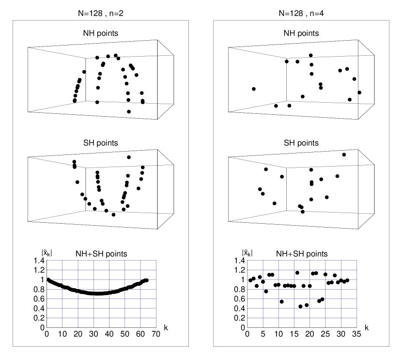
Figure 8: Fuzzy sphere $S_{2}^{N}$ for $N=2\,j+1=128$. The corresponding $N\times N$ matrices $M^{a}$ are defined by (18)–(19). An alternative extraction procedure, with block size $n=2$ (left) and $n=4$ (right), gives emergent spacetime points with coordinates $\widetilde{x}_{k}^{\>a}$, for $a\in\{1,\,2,\,3\}$ and $k=1,\,2\,\ldots\,,\,N/n$, as defined by (25). Shown are the points of the northern hemisphere (NH, $\widetilde{x}_{k}^{\>3}\geq 0$), the points of the southern hemisphere (SH, $\widetilde{x}_{k}^{\>3}<0$), and the modulus $|\widetilde{x}_{k}|$ for all points as defined by (26).

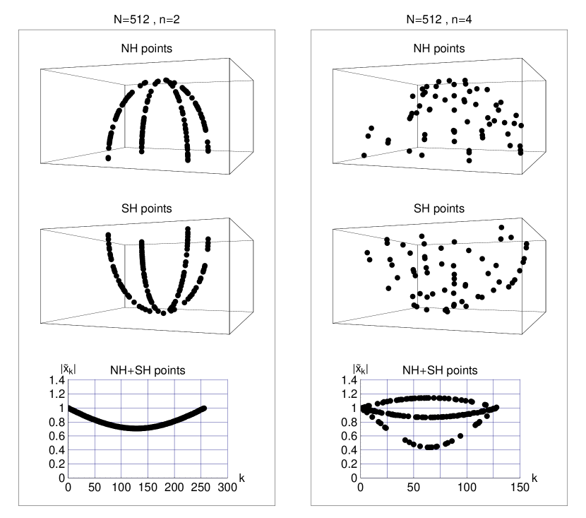
Figure 9: Same as Fig. 8, but now for $N=512$.

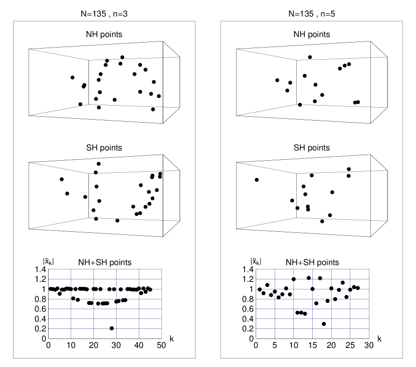
Figure 10: Same as Fig. 8, but now for $N=135$ and $n=3,\,5$.

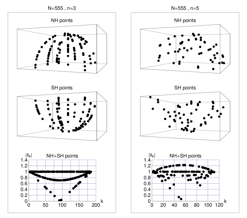
Figure 11: Same as Fig. 8, but now for $N=555$ and $n=3,\,5$.

References

- (1) N. Ishibashi, H. Kawai, Y. Kitazawa, and A. Tsuchiya, “A large- reduced model as superstring,” Nucl. Phys. B 498, 467 (1997), arXiv:hep-th/9612115.
- (2) H. Aoki, S. Iso, H. Kawai, Y. Kitazawa, A. Tsuchiya, and T. Tada, “IIB matrix model,” Prog. Theor. Phys. Suppl. 134, 47 (1999), arXiv:hep-th/9908038.
- (3) S.W. Kim, J. Nishimura, and A. Tsuchiya, “Expanding (3+1)-dimensional universe from a Lorentzian matrix model for superstring theory in (9+1)-dimensions,” Phys. Rev. Lett. 108, 011601 (2012), arXiv:1108.1540.
- (4) J. Nishimura and A. Tsuchiya, “Complex Langevin analysis of the space-time structure in the Lorentzian type IIB matrix model,” JHEP 1906, 077 (2019), arXiv:1904.05919.
- (5) K. Hatakeyama, A. Matsumoto, J. Nishimura, A. Tsuchiya, and A. Yosprakob, “The emergence of expanding space-time and intersecting D-branes from classical solutions in the Lorentzian type IIB matrix model,” Prog. Theor. Exp. Phys. 2020, 043B10 (2020), arXiv:1911.08132.
- (6) F.R. Klinkhamer, “On the emergence of an expanding universe from a Lorentzian matrix model,” preprint arXiv:1912.12229v6.
- (7) F.R. Klinkhamer, “On the emergence of an expanding universe from a Lorentzian matrix model,” Prog. Theor. Exp. Phys. 2020, 103B03 (2020), arXiv:1912.12229.
- (8) F.R. Klinkhamer, “IIB matrix model: Emergent spacetime from the master field,” Prog. Theor. Exp. Phys. 2021, 013B04 (2021), arXiv:2007.08485.
- (9) S. Wolfram, Mathematica: A System for Doing Mathematics by Computer, Second Edition (Addison–Wesley, Redwood City, CA, 1991).
- (10) D.E. Knuth, The Art of Computer Programming, Vol. 2, Seminumerical Algorithms, Third Edition (Addison–Wesley, Reading, Mass, 1998).
- (11) J. Hoppe, “Membranes and matrix models,” arXiv:hep-th/0206192.
- (12) H. Steinacker, “Non-commutative geometry and matrix models,” PoS QGQGS2011, 004 (2011), arXiv:1109.5521.
- (13) A. Connes, “Noncommutative geometry, the spectral standpoint,” arXiv:1910.10407.
- (14) H.C. Steinacker, “On the quantum structure of space-time, gravity, and higher spin in matrix models,” Class. Quant. Grav. 37, 113001 (2020), arXiv:1911.03162.