Implicit automata in typed $\lambda$-calculi II:
streaming transducers vs categorical semantics

Abstract.

We characterize regular string transductions as programs in a linear $\lambda$-calculus with additives. One direction of this equivalence is proved by encoding copyless streaming string transducers (SSTs), which compute regular functions, into our $\lambda$-calculus. For the converse, we consider a categorical framework for defining automata and transducers over words, which allows us to relate register updates in SSTs to the semantics of the linear $\lambda$-calculus in a suitable monoidal closed category.

To illustrate the relevance of monoidal closure to automata theory, we leverage this notion to give abstract generalizations of the arguments showing that copyless SSTs may be determinized and that the composition of two regular functions may be implemented by a copyless SST.

Our main result is then generalized from strings to trees using a similar approach. In doing so, we exhibit a connection between a feature of streaming tree transducers and the multiplicative/additive distinction of linear logic.

1. Introduction

We recently initiated [NP20] a series of works at the interface of programming language theory and automata. As the title suggests, the present paper is the second installment; it starts with an introduction to this research programme, meant to be accessible with a general computer science background (Section 1.1). After stating a main theorem, we shall argue, in two mostly independent subsections, that these connections between two fields that we investigate:

• are relevant to natural questions on the $\lambda$-calculus (Section 1.2);

• provide new conceptual insights into automata theory (Section 1.3).

Section 1.4 exposes some of our key technical ideas, stressing the role of category theory as a mediating language. A table of contents is provided after this introduction.

1.1. What is this all about?

1.1.1. From proofs-as-programs to implicit complexity

One of the central principles in the contemporary theory of programming languages is a close relationship between constructive logics and statically typed functional programming, known as the proofs-as-programs correspondence, also known as the formulae-as-types or Curry–Howard correspondence. The idea is that, in certain logical systems, proofs admit a “normalization procedure” that can be seen as the execution of a program. According to this analogy, a proof is thus a program, and the formula that it proves is the type of the program. A remarkable empirical fact is that this manifests as several concrete isomorphisms between (theoretical) languages and proof systems that were designed independently.

An important point is that termination on the programming side is highly desirable in this context since it entails consistency on the logical side. Take for instance the untyped $\lambda$-calculus, one of the models of computation that led to the birth of computability theory in the 1930s, nowadays used as a theoretical foundation for functional programming. It allows non-terminating programs. The simply typed $\lambda$-calculus adds a type system on top of it; one can then rule out this possibility of non-termination by only allowing well-typed programs, thus ensuring the consistency of the corresponding logical system (here, intuitionistic propositional logic) at the price of losing Turing-completeness.

Such a termination guarantee might even come with quantitative time complexity bounds. For instance, Hillebrand et al. [HKM96] show that programs in the simply typed $\lambda$-calculus operating over certain data encodings and returning booleans can compute all functions in the complexity class $\mathsf{ELEMENTARY}$ (i.e. those with a time complexity bounded by a tower of exponentials), and only those. This result illustrates the type-theoretic approach to implicit computational complexity, a well-established field concerned with machine-free characterizations of complexity classes via high-level programming languages. Many works in this area have taken inspiration from linear logic [Gir87] to design more sophisticated type systems, starting with two characterizations of polynomial time [GSS92, Gir98]. As another example, Linear Logic by Levels [BM10] also characterizes $\mathsf{ELEMENTARY}$ and admits a translation from the simply typed $\lambda$-calculus [GRV09].

1.1.2. Implicit automata

Let us consider strings over some finite alphabet as input. Functions mapping these strings to booleans are equivalent to sets of strings, and the latter are called languages. Complexity classes (of decision problems) are often defined as sets of languages, but such sets also arise in automata theory. A typical example is the class of regular languages, that can be defined by regular expressions or equivalently by finite automata (we assume here that the reader knows about those): usually, it is not considered a complexity class, although this statement is sociological rather than formal.

Our research programme aims to provide for automata what (type-theoretic) implicit complexity has done for complexity classes. A characterization of regular languages had already been obtained by Hillebrand and Kanellakis in the simply typed $\lambda$-calculus [HK96, Theorem 3.4]. Starting from this, we characterized [NP20] the smaller class of star-free languages by relying on a richer type system that supports so-called non-commutative types. As mentioned in [NP20, §7], some other results of this kind already exist, but not many; and as far as we know, the idea of “implicit automata” as a topic worthy of systematic investigation had not been put forth before in writing.

1.1.3. Transducers

Here, our goal is to go beyond languages and to consider string-to-string functions instead. There is a wide variety of classes of such functions that appear in automata theory, and several of them collapse to regular languages when we restrict them to a single output bit (this is the case for the so-called sequential functions, rational functions, regular functions… see the surveys [FR16, MP19]). In other words, many automata models that recognize regular languages are no longer equivalent when extended with the ability to produce an output string. Such automata with output are called transducers. We could therefore expect fine distinctions between the feature sets of various $\lambda$-calculi to be reflected in differences between the string functions that they can express.

Yet we only know of two precedents for string-to-string transduction classes captured using typed functional programming: sequential functions in a cyclic proof system [DP16] and polyregular functions in a $\lambda$-calculus with primitive data types [Boj18, §4]. Both are discussed further in the prequel paper [NP20, §7].

This brings us to our first main theorem:

Theorem 1.

A function $\Sigma^{*}\to\Gamma^{*}$ is $\lambda\ell^{\oplus\with}$-definable if and only if it is regular.

By “$\lambda\ell^{\oplus\with}$-definable”, we mean expressible in the $\lambda\ell^{\oplus\with}$-calculus (a system based on Intuitionistic Linear Logic) in the specific but mostly standard way described in Definition 2.3.3. As for regular functions, they are a well-studied class with many equivalent definitions, for instance two-way transducers or monadic second-order logic [EH01]. We may also point to several recent formalisms [AFR14, DGK18, BDK18] for regular functions using combinators as belonging to “implicit complexity for automata”, albeit not of the type-theoretic kind (implicit complexity is an umbrella term which traditionally also includes tools such as recursive function algebras or term rewriting).

1.2. Internal motivations from typed $\lambda$-calculi

We mentioned earlier a characterization of $\mathsf{ELEMENTARY}$ in the simply typed $\lambda$-calculus by Hillebrand et al. [HKM96]. It uses a somewhat unusual (though perfectly justified) representation for the inputs. The conventional choice would have been the Church encoding of strings. They are indeed the usual tool to represent all computable functions in the untyped $\lambda$-calculus, and in some terminating type systems, any “reasonable” function can still be programmed over these encodings (for example, this is the case for System F [Wad07]). But in the simply typed case, some earlier results by Statman had suggested a hopeless lack of expressiveness (see e.g. the discussion in [FLO83] after its Theorem 4.4.3.). Then Hillebrand and Kanellakis’s aforementioned result [HK96] showed that, surprisingly, one gets the class of regular languages by using Church-encoded strings in the simply typed $\lambda$-calculus!

Recently, the present paper’s first author reused their ideas in [Ngu19] to solve an open problem from “standard” implicit complexity, concerning a characterization of polynomial time by Baillot et al. [BDBRDR18] that makes use of Church encodings. The question was whether a certain feature (namely type fixpoints) was necessary for this result. It turns out [Ngu19] that when this feature is removed, the class of languages obtained is regular languages instead of $\mathsf{P}$.

The moral of the story, for us, is that the use of Church-encoded strings can lead naturally to connections with automata theory. Admittedly, this naturality judgment is inherently subjective. But concretely, it translates into a methodological commitment: we explore the expressiveness of typed $\lambda$-calculi that already exist (perhaps up to a few minor details), whereas it is usual in implicit complexity to engineer some (potentially ad-hoc) new type system to achieve desired complexity effects. Most of the time, the features of these preexisting $\lambda$-calculi have original motivations that are entirely unrelated to complexity or automata (for instance, the non-commutative types that we used in [NP20] originate from the study of natural language [Lam58] and the topology of proofs (see e.g. [Gir89, §II.9.])).

In the case of the simply typed $\lambda$-calculus, characterizing the definable string-to-string functions in the style of [HK96, Theorem 3.4] (again!) is in fact an old open problem (while a more restrictive notion of $\lambda$-definability is well understood [Zai87]). As we are not yet able to solve it, we instead tackle a version where linearity constraints have been added, resulting in Theorem 1. Recall that a function is said to be linear (in the sense of linear logic) when it uses its argument only once. The system that we use to express these constraints is Dual Intuitionistic Linear Logic [Bar96] with additive connectives (called here the $\lambda\ell^{\oplus\with}$-calculus).

1.3. Conceptual interest for (categorical) automata theory

This notion of linearity in programming language theory has a counterpart in the old theme of restricting the copying power of automata models (see e.g. [ERS80]). The latter is manifested in one of the possible definitions of the regular functions mentioned in Theorem 1: copyless streaming string transducers (SSTs) [AČ10]. An SST is roughly speaking an automaton whose internal memory consists of a state (in a finite set) and some string-valued registers, and its transitions are copyless when they compute new register values without duplicating the old ones.

Put this way, Theorem 1 seems unsurprising. But there is more going on behind the scenes. In particular, while it is trivial that the composition of two $\lambda\ell^{\oplus\with}$-definable functions is itself $\lambda\ell^{\oplus\with}$-definable, composing copyless SSTs requires intricate combinatorics as can be seen in [BC18, Chapter 13] for example. As it turns out, the tools developed in order to prove Theorem 1 also yield a clean proof of the closure of copyless streaming string transducers under composition, which it even generalizes using the language of category theory, see below.

Another subtlety comes from our extension of Theorem 1 to ranked trees:

Theorem 2.

Let ${\bf\Sigma}$ and ${\bf\Gamma}$ be ranked alphabets. A function $\mathbf{Tree}({\bf\Sigma})\to\mathbf{Tree}({\bf\Gamma})$ is $\lambda\ell^{\oplus\with}$-definable if and only if it is regular.

The class of regular tree functions is obtained by generalizing the definition for strings based on monadic second-order logic (MSO, see e.g. [BD20]). There is also an automata model adapting SSTs to trees, namely the bottom-up ranked tree transducers (BRTT) [AD17]. However, it is conjectured that some regular functions cannot be computed by copyless BRTTs. Instead, a more sophisticated linearity condition, called the single use restriction, is imposed on BRTTs in [AD17] in order to characterize the regular tree functions. The additional flexibility thus afforded, compared to copyless BRTTs, turns out to correspond directly to an important feature of linear type systems, namely the additive conjunction.

As a concrete manifestation of this correspondence, we conjecture that all tree functions definable in the $\lambda\kern-0.50003pt\mbox{ \hskip 5.00002pt{1 0 0.4 1} \hbox to0.0pt{\hss\leavevmode\hbox{\set@color\text{a}}} }$-calculus of our previous paper [NP20] can be computed by copyless BRTTs. This $\lambda\kern-0.50003pt\mbox{ \hskip 5.00002pt{1 0 0.4 1} \hbox to0.0pt{\hss\leavevmode\hbox{\set@color\text{a}}} }$-calculus does not contain the additive connectives $\with/\oplus$ of linear logic; to compensate, it has an affine type system, instead of a linear one (whence the   1 0 0.4 1 a ). We leave the proof of this fact for future work.

In the case of strings, single-use-restricted streaming string transducers are very close to copyless non-determinstic SSTs. (That additive connectives in linear logic have something to do with non-determinism has previously been observed in other settings, for instance in [MT03].) Their equivalence with copyless SSTs thus corresponds to a determinization theorem, that already has an indirect proof via MSO [AD11]. We provide here a direct construction, whose main technical ingredient is the “transformation forest” data structure applied to copyless SSTs in [BC18, Chapter 13] and reminiscent of the Muller–Schupp determinization [MS95] for automata over infinite words. Most importantly, this determinization result is again formulated in a general category-theoretic setting.

Together with the aforementioned analysis of the composition of SSTs, those are our two contributions to “categorical automata theory”. This kind of use of categories to understand the essence of various constructions on automata – such as determinization or minimization – and to generalize them to other settings has a long history, see for instance [vHKR⁺19] and the many references therein.

1.4. Transducers over monoidal closed categories

Another example of categorical automata theory is the work of Colcombet and Petrişan [CP17a, CP20] on minimization, whose direct relevance to us lies in the categorical framework for automata models that it introduces: objects serve as state spaces and morphisms as transitions. Our technical development takes place in a very similar framework.

• We first define a category $\mathcal{SR}$ that corresponds to single-state copyless SSTs.

• Since copylessness and the so-called single use restriction morally differ by the presence of the additive conjunction ‘$\with$’ of linear logic, we “add ‘$\with$’ freely” to achieve a similar effect: automata in the resulting category $\mathcal{SR}_{\with}$, although not identical to single-state single use restricted SSTs, are easily seen to be equally expressive.

• Finally, we perform another “completion” denoted $(-)_{\oplus}$ to incorporate a finite set of states, so that $\mathcal{SR}_{\oplus}$ (resp. $(\mathcal{SR}_{\with})_{\oplus}$) corresponds to usual – i.e. stateful – copyless (resp. single use restricted) SSTs. (Similar completions by certain colimits have been previously exploited [CP17b] within Colcombet and Petrişan’s framework.)

The linchpin on which the various results previously mentioned rely is:

Theorem 3.

$(\mathcal{SR}_{\with})_{\oplus}$ is a symmetric monoidal closed category (SMCC).

On the one hand, from the point of view of categorical automata theory, an SMCC provides a setting in which constructions relying on function spaces (i.e. internal homsets) can be carried out (this is typically the case when one exploits the finiteness of $Q^{Q}$ for any finite set of states $Q$). This is the case for our composition result, whose general version is stated over arbitrary SMCCs. While $(\mathcal{SR}_{\with})_{\oplus}$ is an SMCC, $\mathcal{SR}_{\oplus}$ is not, and this explains why composing copyless SSTs (that correspond to $\mathcal{SR}_{\oplus}$) directly is difficult: instead, a detour through $(\mathcal{SR}_{\with})_{\oplus}$ allows us to apply Theorem 3. This move from $\mathcal{SR}_{\oplus}$ to $(\mathcal{SR}_{\with})_{\oplus}$ is made possible by our abstract determinization argument, which itself relies on the existence of some (but not all) function spaces in $\mathcal{SR}_{\oplus}$.

On the other hand, for the programming language theorist, the notion of SMCC is an axiomatization of the denotational semantics for the “purely linear” fragment of our $\lambda\ell^{\oplus\with}$-calculus. We can therefore apply a semantic evaluation argument, following a long tradition in implicit complexity (cf. [HK96, Ter12]), to deduce Theorem 1 from Theorem 3; similarly, Theorem 2 follows from the monoidal closure of a category $(\mathcal{TR}_{\with})_{\oplus}$ for trees. (Semantics of linear logic have also been applied to higher-order recursion schemes, a topic at the interface with automata, in [Gre16, Mel17, CM19], as well as to the purely automata-theoretic Church synthesis problem in some publications [PR18, PR19] coauthored by the present paper’s third author.) That said, to create suitable conditions for semantic evaluation, a quite lengthy syntactic analysis is required, with the presence of positive connectives in the $\lambda\ell^{\oplus\with}$-calculus causing some complications.

At this point, we must mention the kinship of this $(\mathcal{SR}_{\with})_{\oplus}$ with one of the earliest denotational models of linear logic, the Dialectica categories [dP89] (originating as a categorical account of Gödel’s “Dialectica” functional interpretation [Göd58]). Composing the free finite coproduct completion $(-)_{\oplus}$ with its dual product completion $(-)_{\with}$ is indeed reminiscent of a factorization into free sums and free products of a generalized Dialectica construction [Hof11]. Thus, Theorem 3 holds for reasons similar to those for the monoidal closure of Dialectica categories (with a function space formula that resembles the interpretation of implication in [Göd58]). Such Dialectica-like structures have appeared in quite varied contexts in the past few years, such as lenses from functional programming and compositional game theory (see e.g. [Hed18, §4] for both), and, more in line with the topic of this paper, the aforementioned works on Church’s synthesis [PR18, PR19] (and a closely related work on automata over infinite trees [Rib20]).

To wrap up this introduction, let us mention that as a bridge between $\lambda\ell^{\oplus\with}$-definability and those automata models, we also define within our categorical framework a notion of transducer whose memory is made up of (purely linear) $\lambda\ell^{\oplus\with}$-terms. This idea of using linear $\lambda$-terms inside a transducer model also appears in a recent characterization of regular tree functions [GLS20].

2. Preliminaries

2.1. Notations & elementary definitions

2.1.1. Sets and categories

The cardinality of a set $X$ is written ${|X|}$. We sometimes consider a family $(x_{i})_{i\in I}$ as a map $i\mapsto x_{i}$, which amounts to treating $\prod_{i\in I}X_{i}$ as a dependent product. Consistently with this, we make use of the dependent sum operation

$$\sum_{i\in I}X_{i}=\{(i,x)\mid i\in I,\,x\in X_{i}\}$$

We (seldom) write numerals $n$ for the underlying sets $\{0,\ldots,n-1\}$ for conciseness.

Given a category $\mathcal{C}$, we write $\mathsf{Obj}(\mathcal{C})$ for its class of objects and $\mathsf{Hom}_{\mathcal{C}}\left(A,B\right)$ for the set of arrows (or morphisms) from $A$ to $B$ (for $A,B\in\mathsf{Obj}(C)$). The composition of two morphisms $f\in\mathsf{Hom}_{\mathcal{C}}\left(A,B\right)$ and $g\in\mathsf{Hom}_{\mathcal{C}}\left(B,C\right)$ is denoted by $g\circ f$. Following the traditional notations of linear logic, products and coproducts will be customarily written using ‘$\with$’ and ‘$\oplus$’ respectively – except in the category of sets where we use the notations ‘$\times$’ and ‘$+$’ as usual – and we reserve $\top$ for the terminal object. We sometimes use basic combinators such as $\left\langle-\right\rangle$/$[-]$ for pairing/copairing and $\pi_{i}$/${\sf in}_{i}$ for projections/coprojections. With these notations, recall that the binary coproduct of sets is the tagged union

$$X+Y=\{\mathsf{in}_{1}(x)\mid x\in X\}\cup\{\mathsf{in}_{2}(y)\mid y\in Y\}$$

The injection $\mathsf{in}_{1}/\mathsf{in}_{2}$ may be omitted by abuse of notation when it is clear from the context, that is, for $x\in X$, we allow ourselves to write $x$ for $\mathsf{in}_{1}(x)$ when it is understood that this refers to an element of $X+Y$.

Finally, if we are given a binary operation $\square$ over the objects of a category, we freely use the corresponding “$I$-ary” operation, with a notation of the form $\bigbox_{i\in I}A_{i}$, over families indexed by a finite set $I$. Concretely speaking, this depends on a fixed total order over $I=\{i_{1}<\ldots<i_{{|I|}}\}$ to unfold as $A_{i_{1}}\,\square\,(A_{i_{2}}\,\square\,(\ldots\,\square\,A_{i_{{|I|}}})\ldots)$ – for convenience, the reader may consider that a choice of such an order for every finite set is fixed once and for all for the rest of the paper. In practice, the particular order does not matter since we will deal with operations $\square\in\{\oplus,\with,\otimes,\dots\}$ that are symmetric in a suitable sense. Those operations also have units (i.e. identity elements), giving a canonical meaning to $\bigoplus_{i\in\varnothing}A_{i}$, $\bigwith_{i\in\varnothing}A_{i}$, etc.

Finally, as is usual when dealing with categories, we sometimes allow ourselves to implicitly use the axiom of choice for classes to pick objects determined by their universal properties to build functors (for instance, given an object $A$ in a category $\mathcal{C}$ with cartesian products, we shall speak of the functor $-\with A$ without first mentioning that a choice of cartesian products $X\with A$ exists for for every $X$ in $\mathcal{C}$). This is merely for convenience; the reader may check that in all of our concrete examples of interest, canonical choices can be made without appealing to choice.

2.1.2. Strings and ranked trees

Alphabets designate finite sets and are written using the variable names $\Sigma,\Gamma$. The set of strings (or words) over an alphabet $\Sigma$ is denoted by $\Sigma^{*}$. The concatenation of two strings $u,v\in\Sigma^{*}$ is written $uv$ (or sometimes $u\cdot v$ for clarity); recall that $\Sigma^{*}$ endowed with this operation is the free monoid over the set of generators $\Sigma$, and its identity element is the empty string $\varepsilon$. We write ${|w|}$ for the length of a word $w\in\Sigma^{*}$, and given a letter $c\in\Sigma$, the notation $|w|_{c}$ refers to the number of occurrences of $c$ in $w$.

Ranked alphabets are pairs $(\Sigma,\mathrm{ar})$ such that $\Sigma$ is an alphabet and the arity $\mathrm{ar}$ is a family of finite sets indexed by $\Sigma$; they are written using $\bf\Sigma,\Gamma$. We may write $\{a_{1}:A_{1},\;\ldots,\;a_{n}:A_{n}\}$ for the ranked alphabet $(\{a_{1},\ldots,a_{n}\},\mathrm{ar})$ with $\mathrm{ar}(a_{i})=A_{i}$.

Given a ranked alphabet $\bf\Sigma$, the set $\mathbf{Tree}({\bf\Sigma})$ of trees/terms over a ranked alphabet $\bf\Sigma$ is defined as usual: if $a$ is a letter of arity $X$ in $\bf\Sigma$ and $t$ a family of $\bf\Sigma$-trees, we write $a(t)$ for the corresponding tree. Examples of such trees are pictured in Figure 1.

Remark 4.

Given an alphabet $\Sigma$, define $\overline{\Sigma}$ to be the ranked alphabet $(\Sigma+\{\varepsilon\},\mathrm{ar})$ such that $\mathrm{ar}(\mathsf{in}_{1}(a))=\{*\}$ and $\mathrm{ar}(\mathsf{in}_{2}(\varepsilon))=\varnothing$. This gives a isomorphism $\mathbf{Tree}(\overline{\Sigma})\simeq\Sigma^{*}$, illustrated on the right of Figure 1.

 

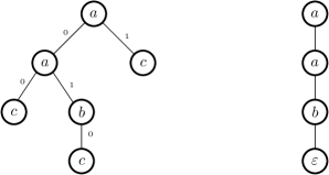
Figure 1. Graphical representations of the tree $a(a(c,b(c)),c)$ over the ranked alphabet $\{a:\{0,1\},\,b:\{0\},\,c:\varnothing\}$ (left) and of the word $aab\in\{a,b\}^{*}$ seen as an element of $\mathbf{Tree}(\overline{\{a,b\}})=\mathbf{Tree}({\{a:\{*\},\,b:\{*\},\,\varepsilon:\varnothing\}})$ (right).

2.2. Transducer models for regular functions over strings and trees

2.2.1. Strings

Let us first recall the machine model that provides our reference definition for regular functions: copyless streaming string transducers [AČ10] (SSTs). A SST is an automaton whose internal memory contains, additionally to its control state, a finite number of string-valued registers. It processes its input in a single left-to-right pass. Each time a letter is read, the contents of the registers may be recombined by concatenation to determine the new register values. Formally:

Fix a finite alphabet $\Gamma$. Let $R$ and $S$ be finite sets; we shall consider their elements to be “register variables”.

A $\Gamma$-register transition from $R$ to $S$ is a function $t:S\to(\Gamma+R)^{*}$. Such a transition is said to be copyless when for every $r\in R$, there is at most one occurrence of $\mathsf{in}_{2}(r)$ among all the words $t(s)$ for $s\in S$ (i.e. when $\sum_{s\in S}|t(s)|_{\mathsf{in}_{2}(r)}\leq 1$). We write $[R\to_{\mathcal{SR}(\Gamma)}S]$ for the set of copyless $\Gamma$-register transitions from $R$ to $S$, or $[R\to_{\mathcal{SR}}S]$ when $\Gamma$ is clear from context.

Let $t\in[R\to_{\mathcal{SR}(\Gamma)}S]$. For $x=(x_{r})_{r\in R}\in(\Gamma^{*})^{R}$ and $s\in S$, we denote by $(t^{\dagger}(x))_{s}\in\Gamma^{*}$ the word obtained from $t(s)$ by substituting every occurrence of a register variable $r\in R$ by the string $x_{r}$ – formally, by applying the morphism of free monoids $(\Gamma+R)^{*}\to\Gamma^{*}$ that maps $\mathsf{in}_{1}(c)$ to $c$ and $\mathsf{in}_{2}(r)$ to $x_{r}$. This defines a set-theoretic map $t^{\dagger}:(\Gamma^{*})^{R}\to(\Gamma^{*})^{S}$, describing how $t$ acts on tuples of strings.

For instance, $t:z\mapsto axby$ (where we omitted $\mathsf{in}_{1}/\mathsf{in}_{2}$) is in $[\{x,y\}\to_{\mathcal{SR}(\{a,b\})}\{z\}]$ (it is copyless since $x$ and $y$ appear only once), and $t^{\dagger}(x\mapsto b,\,y\mapsto aa)=(z\mapsto abbaa)$.

[[AČ10]] A (deterministic) copyless streaming string transducer (SST) with input alphabet $\Sigma$ and output alphabet $\Gamma$ is a tuple $\mathcal{T}=(Q,q_{0},R,\delta,i,o)$ where

• $Q$ is a finite set of states and $q_{0}\in Q$ is the initial state;

• $R$ is a finite set of registers;

• $\delta:\Sigma\times Q\to Q\times[R\to_{\mathcal{SR}(\Gamma)}R]$ is the transition function;

• $i\in[\varnothing\to_{\mathcal{SR}(\Gamma)}R]\cong(\Gamma^{*})^{R}$ describes the initial register values;

• $o:Q\to[R\to_{\mathcal{SR}(\Gamma)}\{\bullet\}]$ (where $\bullet$ is an arbitrary element) describes how to recombine the final values of the registers, depending on the final state, to produce the output.

(The SSTs that we consider in this paper are always copyless.)

The function $\Sigma^{*}\to\Gamma^{*}$ computed by $\mathcal{T}$ maps an input string $w=w_{1}\ldots w_{n}\in\Sigma^{*}$ to the output string $o(q_{n})^{\dagger}\circ t^{\dagger}_{n}\circ\ldots\circ t^{\dagger}_{1}\circ i^{\dagger}(\varnothing)\in\Gamma^{*}$ where

• the empty family $\varnothing$ is indeed the unique element of $(\Gamma^{*})^{\varnothing}$;

• the codomain $(\Gamma^{*})^{\{\bullet\}}$ of $o^{\dagger}(q_{n})$ is identified with $\Gamma^{*}$;

• the register transitions $(t_{i})_{1\leq i\leq n}$ and the final state $q_{n}\in Q$ are inductively defined, starting from the fixed initial state $q_{0}$, by $(q_{i},t_{i})=\delta(w_{i},q_{i-1})$.

The functions that can be computed by copyless SSTs are called regular string functions.

$$\small\begin{array}[]{rcl!{\hspace{15em}} l}(\Sigma\sqcup\{{\|}\})^{*}&\to&\Sigma^{*}\hfil\lx@intercol\hskip 135.00023pt&{(w_{i}\in\Sigma^{*},\;(\Sigma\sqcup\{\|\})^{*}\cong\Sigma^{*}(\|\Sigma^{*})^{*})}\\ w_{0}&\mapsto&\varepsilon\hfil\lx@intercol\hskip 135.00023pt\\ w_{0}\|\ldots\|w_{2k}&\mapsto&\lx@intercol\mathtt{reverse}(w_{2k-1})\mathtt{reverse}(w_{2k-3})\ldots\mathtt{reverse}(w_{1})w_{0}w_{2}\ldots w_{2k-2}\hfil\lx@intercol\\ w_{0}\|\ldots\|w_{2k+1}&\mapsto&\varepsilon\hfil\lx@intercol\hskip 135.00023pt\\ \end{array}$$

 

Figure 2. An informal depiction of a SST and the induced map $(\Sigma\sqcup\{\|\})^{*}\to\Sigma^{*}$.

Let us describe a simple copyless SST with $\Sigma=\Gamma$ and a single state, so that $\delta:\Sigma\to[R\to_{\mathcal{SR}}R]$. We take $R=\{x,y\}$; both $x$ and $y$ are initialized with the empty string $\varepsilon$, and the register transition $t_{c}=\delta(c)\in[R\to_{\mathcal{SR}}R]$ associated to $c\in\Sigma$ is $(x\mapsto xc,\,y\mapsto cy)$ (to be pedantic, one should write $(x\mapsto\mathsf{in}_{2}(x)\mathsf{in}_{1}(c),\,y\mapsto\mathsf{in}_{1}(c)\mathsf{in}_{2}(y))$). Then for $w=w[1]\ldots w[n]\in\Sigma^{*}$, we have:

$$t_{w[n]}^{\dagger}\circ\dots\circ t_{w[1]}^{\dagger}(x\mapsto\varepsilon,\,y\mapsto\varepsilon)=(x\mapsto w,\,y\mapsto\mathtt{reverse}(w))$$

If we take $o=xy$ (via the canonical isomorphism $[R\to_{\mathcal{SR}(\Gamma)}1]^{\{q\}}\cong(\Gamma+R)^{*}$), the function computed by the SST is $w\in\Sigma^{*}\mapsto w\cdot\mathtt{reverse}(w)$. Figure 2 shows a more sophisticated SST with two states and the associated regular function.

2.2.2. Trees as output

Let us briefly discuss the challenges that arise when extending this model to handle ranked trees instead of strings. We will revisit this material in more detail in Section 5.

The notion of regular tree-to-tree function is defined by generalizing the characterization of regular string functions by Monadic Second-Order Logic [EM99, BE00, EH01], in a way that is compatible with the above isomorphism. There are two orthogonal difficulties that have to be overcome to define a SST-like model for regular tree functions: one comes from producing trees as output, while the other comes from taking trees as input. Bottom-up ranked tree transducers (BRTTs) [AD17] (and the similar model of register tree transducers in [BD20, §4]) provide solutions for both.

String-to-tree regular functions require a modification of the kind of data stored in the registers of an SST. Tree-valued registers are not enough, for the following reasons: to recover the flexibility of string concatenation, one should be able to perform operations such as grafting the root of some tree to a leaf of another tree; but then the latter should be a tree with a distinguished leaf, serving as a “hole” waiting to be substituted by a tree. (This is fundamental in the theory of forest algebras, which proposes various counterparts for trees to the monoid of strings with concatenation, see [Boj].) By allowing both trees and “one-hole trees” as register values, with the appropriate notion of copyless register transition (cf. Section 5.3), one gets the copyless streaming string-to-tree transducers, whose expressive power corresponds exactly to the regular functions [AD17, Theorem 3.16].

2.2.3. Trees as inputs

To compute tree-to-tree regular functions, the first idea would be to blend the notion of copyless SST with the classical bottom-up tree automata. One would then get copyless bottom-up ranked tree transducers. However, this model is believed to be too weak to express all regular tree functions (even in the case of tree-to-string functions). An explicit counterexample is conjectured in [AD17, §2.3], in the case of regular functions on unranked trees; we adapt it here into a function from ranked trees to strings.

In the example below, for a ranked letter $a$ of arity $\mathbbl{2}=\{\triangleleft,\triangleright\}$, we use the abbreviation $a(t,u)$ for $a(\triangleleft\mapsto t,\,\triangleright\mapsto u)$.

[“Conditional swap”] Define $f:\mathbf{Tree}(\{a:\mathbbl{2},b:\mathbbl{2},c:\varnothing\})\to\{a,b,c\}^{*}$ by

$$f(a(t,u))=f(u)\cdot a\cdot f(t)\qquad f(t)=\mathtt{inorder}(t)\ \text{if $t$ doesn't match the previous pattern}$$

where $\mathtt{inorder}$ prints the nodes of $t$ following a depth-first in-order traversal. In other words, $f=\mathtt{inorder}\circ g$ where $g(a(t,u))=a(g(u),g(t))$ and $g(t)=t$ otherwise (i.e. when the root of $t$ is either $b$ or $c$).

Conjecture 5 (adapted from [AD17, §2.3]).

The above $f$ cannot be computed by a copyless BRTT.

One must then allow more register transitions than the copyless ones. This cannot be done haphazardly, for arbitrary register transitions would lead to a much larger class of functions than regular tree functions. Alur and D’Antoni call their relaxed condition [AD17] the single use restriction (it will only be formally defined in Section 5.4); the following single-state BRTT for $f$ provides a typical example of the new possibilities allowed.

[Non-copyless BRTT for conditional swap] Take $R=\{x,y\}$, initialized at the $c$-labeled leaves with $(x\mapsto c,\,y\mapsto c)$. At a subtree $a(u,v)$, we need to combine the registers $x_{\triangleleft},y_{\triangleleft}$ (resp. $x_{\triangleright},y_{\triangleright}$) coming from the left (resp. right) child $u$ (resp. $v$) to produce the values of the registers $x,y$ at this node: this is performed by a register transition

$$t_{a}\in[\{x_{\triangleleft},y_{\triangleleft},x_{\triangleright},y_{\triangleright}\}\to_{\mathcal{SR}}\{x,y\}]\qquad t_{a}(x)=x_{\triangleright}ax_{\triangleleft}\qquad t_{a}(y)=y_{\triangleleft}ay_{\triangleright}$$

The idea is that the register values produced by processing a subtree $u$ are $f(u)$ for $x$ and $\mathtt{inorder}(u)$ for $y$. The register transition for a $b$-labeled node is then $t_{b}(x)=t_{b}(y)=y_{\triangleleft}by_{\triangleright}$, reflecting the fact that $f(b(u,v))=\mathtt{inorder}(b(u,v))$.

This $t_{b}$ is not copyless since $y_{\triangleleft}$ occurs twice: once in $t_{b}(x)$ and once in $t_{b}(y)$. The observation at the heart of the single use restriction is that the values of $x$ and $y$ for a given subtree can never be combined in the same expression in the remainder of the BRTT’s run, so that allowing this duplication of $y_{\triangleleft}$ will never lead to having two copies of $y_{\triangleleft}$ inside the value of a single register. We will see much later in Example 5.4 that this BRTT is indeed single-use-restricted.

2.3. The $\lambda\ell^{\oplus\with}$-calculus, encodings of strings/trees, and definability of functions

2.3.1. Types & terms

We consider a linear $\lambda$-calculus which we dub the $\lambda\ell^{\oplus\with}$-calculus, based (via the Curry–Howard correspondence) on propositional intuitionistic linear logic with both multiplicative and additive connectives (IMALL) together with a base linear type $\mathbbl{o}$. The grammar of types is as follows:

$$\tau,\sigma\mathrel{::=}\mathbbl{o}\;|\;\tau\multimap\sigma\;|\;\tau\otimes\sigma\;|\;\mathbf{I}\;|\;\tau\to\sigma\;|\;\tau\with\sigma\;|\;\tau\oplus\sigma\;|\;\top\;|\;0$$

A typing context $\Psi$ is a finite set of declarations $x_{1}:\tau_{i},\ldots,x_{k}:\tau_{k}$ where the $x_{i}$ are pairwise distinct variables (which constitute the set of free variables of $\Psi$) and the $\tau_{i}$ are types. Typed $\lambda\ell^{\oplus\with}$-terms are given in Figure 3 along with the inductive definition of the typing judgment $\Psi;\;\Delta\vdash t:\tau$, where $\Psi$ and $\Delta$ are contexts (with disjoint sets of free variables), $\tau$ is a type and $t$ is a term. In such a judgment, $\Psi$ is called the non-linear context and $\Delta$ the linear context; the basic idea is that variables in $\Psi$ may be used arbitrarily many times, while those in $\Delta$ must be used exactly once. This is formally more restrictive than an affineness condition, where we would rather restrict variables in $\Delta$ to occur at most once in $t$.

In practice, $\lambda\ell^{\oplus\with}$ is not less expressive than its affine variant since it features additives: the basic idea is that the affineness can be encoded at the level of types by using the linear type $\tau\with\mathbf{I}$ instead of the affine type $\tau$ (as argued for instance in [Gir95, §1.2.1]).

The simply typed $\lambda$-calculus admits an embedding into $\lambda\ell^{\oplus\with}$. Conversely, there is a mapping from $\lambda\ell^{\oplus\with}$ to the simply typed $\lambda$-calculus with products and sums by “forgetting linearity” (and replacing the tensorial product eliminator ${\mathsf{let}}\;{x\otimes y}={t}\;{\mathsf{in}}\;{u}$ by the variant based on projections $u[\pi_{1}(t)/x,\pi_{2}(t)/y]$).

$$\begin{array}[]{c !{\quad} c}\dfrac{}{\Psi;\;x:\tau\vdash x:\tau}&\dfrac{}{\Psi,x:\tau;\;\cdot\vdash x:\tau}\\ \\ \dfrac{\Psi;\;\Delta,\;x:\tau\vdash t:\sigma}{\Psi;\;\Delta\vdash\lambda x.t:\tau\multimap\sigma}&\dfrac{\Psi;\;\Delta\vdash t:\tau\multimap\sigma\qquad\Psi;\;\Delta^{\prime\prime}\vdash u:\tau}{\Psi;\;\Delta,\;\Delta^{\prime}\vdash t\;u:\sigma}\\ \\ \dfrac{\Psi,\;x:\tau;\;\Delta\vdash t:\sigma}{\Psi;\;\Delta\vdash\lambda^{\oc}x.t:\tau\to\sigma}&\dfrac{\Psi;\;\Delta\vdash t:\tau\to\sigma\qquad\Psi;\;\cdot\vdash u:\tau}{\Psi;\;\Delta\vdash t\;u:\sigma}\\ \\ \dfrac{\Psi;\;\Delta\vdash t:\tau\qquad\Psi;\;\Delta^{\prime}\vdash u:\sigma}{\Psi;\;\Delta,\;\Delta^{\prime}\vdash t\otimes u:\tau\otimes\sigma}&\dfrac{\Psi;\;\Delta^{\prime}\vdash u:\tau\otimes\sigma\qquad\Psi;\;\Delta,x:\tau,y:\sigma\vdash t:\kappa}{\Psi;\;\Delta,\;\Delta^{\prime}\vdash{\mathsf{let}}\;{x\otimes y}={u}\;{\mathsf{in}}\;{t}:\kappa}\\ \\ \dfrac{}{\Psi;\;\cdot\vdash():\mathbf{I}}&\dfrac{\Psi;\;\Delta\vdash t:\mathbf{I}\qquad\Psi;\;\Delta^{\prime}\vdash u:\tau}{\Psi;\;\Delta,\;\Delta^{\prime}\vdash{\mathsf{let}}\;{()}={t}\;{\mathsf{in}}\;{u}:\tau}\\ \\ \\ \dfrac{\Psi;\;\Delta\vdash t:\tau\qquad\Psi;\;\Delta\vdash u:\sigma}{\Psi;\;\Delta\vdash\left\langle t,u\right\rangle:\tau\with\sigma}&\dfrac{\Psi;\;\Delta\vdash t:\tau\with\sigma}{\Psi;\;\Delta\vdash\pi_{1}(t):\tau}\qquad\dfrac{\Psi;\;\Delta\vdash t:\tau\with\sigma}{\Psi;\;\Delta\vdash\pi_{2}(t):\sigma}\\ \\ \\ \lx@intercol\hfil\dfrac{\Psi;\;\Delta\vdash t:\tau}{\Psi;\;\Delta\vdash\mathsf{in}_{1}(t):\tau\oplus\sigma}\qquad\dfrac{\Psi;\;\Delta\vdash t:\sigma}{\Psi;\;\Delta\vdash\mathsf{in}_{2}(t):\tau\oplus\sigma}\hfil\lx@intercol\\ \\ \lx@intercol\hfil\dfrac{\Psi;\;\Delta,x:\tau\vdash u:\kappa\qquad\Psi;\;\Delta,x:\tau\vdash v:\kappa\qquad\Psi;\;\Delta^{\prime}\vdash t:\tau\oplus\sigma}{\Psi;\;\Delta,\Delta^{\prime}\vdash{\mathsf{case}}(t,x.u,x.v):\kappa}\hfil\lx@intercol\\ \\ \dfrac{}{\Psi;\;\Delta\vdash\left\langle\right\rangle:\top}&\dfrac{\Psi;\;\Delta\vdash t:0}{\Psi;\;\Delta,\;\Delta^{\prime}\vdash{\mathsf{abort}}(t):\tau}\end{array}$$

Figure 3. Typing rules of $\lambda\ell^{\oplus\with}$.

$$\footnotesize\begin{array}[]{l !\; c !{\;\;} c}\text{$\beta$-equivalence}&(\lambda x.t)\;u\leavevmode\nobreak\ =_{\beta}\leavevmode\nobreak\ t[u/x]&(\lambda^{\oc}x.t)\;u\leavevmode\nobreak\ =_{\beta}\leavevmode\nobreak\ t[u/x]\\ &\pi_{1}(\left\langle t,u\right\rangle)\leavevmode\nobreak\ =_{\beta}\leavevmode\nobreak\ t&\pi_{2}(\left\langle t,u\right\rangle)\leavevmode\nobreak\ =_{\beta}\leavevmode\nobreak\ u\\ &{\mathsf{case}}(\mathsf{in}_{1}(t),x.u,x.v)\leavevmode\nobreak\ =_{\beta}\leavevmode\nobreak\ u[t/x]&{\mathsf{case}}(\mathsf{in}_{2}(t),x.u,x.v)\leavevmode\nobreak\ =_{\beta}\leavevmode\nobreak\ v[t/x]\\ &{\mathsf{let}}\;{x\otimes y}={t\otimes u}\;{\mathsf{in}}\;{v}\leavevmode\nobreak\ \leavevmode\nobreak\ =_{\beta}\leavevmode\nobreak\ \leavevmode\nobreak\ v[t/x][u/y]&{\mathsf{let}}\;{()}={()}\;{\mathsf{in}}\;{t}\leavevmode\nobreak\ =_{\beta}\leavevmode\nobreak\ t\\ \\ \text{$\eta$-equivalence}&\lambda x.t\;x\leavevmode\nobreak\ =_{\eta}\leavevmode\nobreak\ t&\lambda^{\oc}x.t\;x\leavevmode\nobreak\ =_{\eta}\leavevmode\nobreak\ t\\ &{\mathsf{let}}\;{x\otimes y}={t}\;{\mathsf{in}}\;{u[x\otimes y/z]}\leavevmode\nobreak\ \leavevmode\nobreak\ =_{\eta}\leavevmode\nobreak\ \leavevmode\nobreak\ u[t/z]&\left\langle\pi_{1}(t),\pi_{2}(t)\right\rangle\leavevmode\nobreak\ =_{\eta}\leavevmode\nobreak\ t\\ &{\mathsf{let}}\;{x\otimes y}={t}\;{\mathsf{in}}\;{v[u/z]}\leavevmode\nobreak\ =_{\eta}\leavevmode\nobreak\ v[{\mathsf{let}}\;{x\otimes y}={t}\;{\mathsf{in}}\;{u}/z]&x\leavevmode\nobreak\ =_{\eta}\leavevmode\nobreak\ \left\langle\right\rangle\\ &{\mathsf{let}}\;{()}={t}\;{\mathsf{in}}\;{u[()/z]}\leavevmode\nobreak\ \leavevmode\nobreak\ =_{\eta}\leavevmode\nobreak\ \leavevmode\nobreak\ u[t/z]\\ &{\mathsf{let}}\;{()}={t}\;{\mathsf{in}}\;{v[u/z]}\leavevmode\nobreak\ =_{\eta}\leavevmode\nobreak\ v[{\mathsf{let}}\;{()}={t}\;{\mathsf{in}}\;{u}/z]\\ &{\mathsf{case}}(t,x.u[\mathsf{in}_{1}(x)/z],y.u[\mathsf{in}_{2}(y)/z])\leavevmode\nobreak\ =_{\eta}\leavevmode\nobreak\ u[t/z]&{\mathsf{abort}}(t)\leavevmode\nobreak\ =_{\eta}\leavevmode\nobreak\ u\end{array}$$

Figure 4. Equations for $\lambda\ell^{\oplus\with}$-terms (relating terms that have matching types).

As usual, we identify $\lambda\ell^{\oplus\with}$-terms up to renaming of bound variables ($\alpha$-equivalence) and admit the standard definition of the capture-avoiding substitution. For the purpose of this paper, since we are not interested in the fine details of their operational semantics, we usually consider $\lambda\ell^{\oplus\with}$-terms up to ${\beta\eta}$-equivalence $=_{{\beta\eta}}$ as generated by the equations in Figure 4 and congruence. Note that those equations are implicitly typed and that typing is invariant under ${\beta\eta}$-equivalence.

Much like any $\lambda$-calculus, $\lambda\ell^{\oplus\with}$ can be seen as a programming language by considering a reduction relation $\to_{\beta\varepsilon}$, which happens to be included in $=_{\beta\eta}$. One property that we shall use is that $\lambda\ell^{\oplus\with}$ is normalizing, i.e., that the relation $\to_{\beta\varepsilon}$ is terminating. This allows to consider terms of very specific shape when working up to $\beta\eta$. While the argument is routine, we need this result, as well as a fine-grained understanding of the normal forms to discuss further preliminary syntactic lemmas, so we give an outline in Appendix B.

We now isolate an important class of types and terms for the sequel. We call a type purely linear if it does not have any occurrence of the ‘$\to$’ connective. A $\lambda\ell^{\oplus\with}$-term $t$ is also called purely linear if there is a typing derivation $\Psi;\;\Delta\vdash t:\tau$ where any type occurring must be purely linear.

Intuitively, purely linear terms are those which are not allowed to duplicate any arguments involving $\mathbbl{o}$. For any type derivation $\Psi;\;\Delta\vdash t:\tau$, if the types occurring in $\Psi$ and $\Delta$, as well as $\tau$, are purely linear, then so is $t$; this is a consequence of normalization.

2.3.2. Church encodings

In order to discuss string (and tree) functions in $\lambda\ell^{\oplus\with}$, we need to discuss how they are encoded. Recall that in the pure (i.e. untyped) $\lambda$-calculus, the canonical way to encode inductive types is via Church encodings. Such encodings are typable in the simply-typed $\lambda$-calculus. For instance, for natural numbers and strings over $\{a,b\}$, writing $\underline{w}$ for the Church encoding of $w$, we have

$$\begin{array}[]{clc}\mathrm{Nat}^{\oc}\leavevmode\nobreak\ =\leavevmode\nobreak\ (\mathbbl{o}\to\mathbbl{o})\to\mathbbl{o}\to\mathbbl{o}&&\mathrm{Str}^{\oc}_{\{a,b\}}\leavevmode\nobreak\ =\leavevmode\nobreak\ (\mathbbl{o}\to\mathbbl{o})\to(\mathbbl{o}\to\mathbbl{o})\to\mathbbl{o}\to\mathbbl{o}\\ \\ \underline{3}=\lambda^{\oc}s.\lambda^{\oc}z.s\;(s\;(s\;z))&&\underline{aab}=\lambda^{\oc}a.\lambda^{\oc}b.\lambda^{\oc}\varepsilon.a\;(a\;(b\;\varepsilon))\\ \end{array}$$

Conversely, one may show that any closed simply typed $\lambda$-term of type $\mathrm{Nat}^{\oc}$ (resp. $\mathrm{Str}^{\oc}_{\{a,b\}}$) is ${\beta\eta}$-equivalent to the Church encoding of some number (resp. string). In the rest of this paper, we will use a less common, but more precise $\lambda\ell^{\oplus\with}$-type for Church encodings of strings of trees, first introduced in [Gir87, §5.3.3].

Let $\Sigma$ be an alphabet. We define $\mathrm{Str}_{\Sigma}$ as $(\mathbbl{o}\multimap\mathbbl{o})\to\ldots\to(\mathbbl{o}\multimap\mathbbl{o})\to\mathbbl{o}\to\mathbbl{o}$ where there are ${|\Sigma|}$ occurrences of $\mathbbl{o}\multimap\mathbbl{o}$. Note in particular that thanks to the isomorphism $(A\with B)\to C\;\cong\;A\to B\to C$ (non-linear currying), we have

$$\mathrm{Str}_{\Sigma}\leavevmode\nobreak\ \leavevmode\nobreak\ \cong\leavevmode\nobreak\ \leavevmode\nobreak\ \left(\bigwith_{a\in\Sigma}(\mathbbl{o}\multimap\mathbbl{o})\right)\to\mathbbl{o}\to\mathbbl{o}$$

It can be checked that $\mathrm{Str}_{\Sigma}$ has the same (up to $\beta\eta$ equality) closed inhabitants as the usual $\mathrm{Str}^{\oc}_{\Sigma}$ presented above, but one should keep in mind that this choice is not entirely innocuous. It is in large part motivated by our main result (Theorem 1), which might no longer hold when taking $\mathrm{Str}^{\oc}_{\Sigma}$ instead of $\mathrm{Str}_{\Sigma}$.

This situation generalizes to trees. For instance, the Church encoding of the tree depicted in Figure 1 is $\lambda^{\oc}a.\lambda^{\oc}b.\lambda^{\oc}c.\;a\;(a\;c\;(b\;c))\;c\leavevmode\nobreak\ :\leavevmode\nobreak\ (\mathbbl{o}\to\mathbbl{o}\to\mathbbl{o})\to(\mathbbl{o}\to\mathbbl{o})\to\mathbbl{o}\to\mathbbl{o}$.

Given a ranked alphabet ${\bf\Sigma}=(\Sigma,\mathrm{ar})$, the $\lambda\ell^{\oplus\with}$ type $\mathrm{Tree}_{\bf\Sigma}$ is defined as

$$\mathrm{Tree}_{\bf\Sigma}\leavevmode\nobreak\ \leavevmode\nobreak\ =\leavevmode\nobreak\ \leavevmode\nobreak\ (\mathbbl{o}\multimap\ldots\multimap\mathbbl{o})\to\ldots\to(\mathbbl{o}\multimap\ldots\multimap\mathbbl{o})\to\mathbbl{o}$$

where there are ${|\Sigma|}$ top-level arguments, and, within the component corresponding to the letter $a\in\Sigma$, there are ${|\mathrm{ar}(a)|}$. In other words, we have the isomorphism

$$\mathrm{Tree}_{\bf\Sigma}\leavevmode\nobreak\ \leavevmode\nobreak\ \cong\leavevmode\nobreak\ \leavevmode\nobreak\ \left(\bigwith_{a\in\Sigma}(\mathbbl{o}^{\otimes\mathrm{ar}(a)}\multimap\mathbbl{o})\right)\to\mathbbl{o}$$

Remark 6.

The isomorphism of Remark 4 translates to an equality $\mathrm{Str}_{\Sigma}=\mathrm{Tree}_{\overline{\Sigma}}$.

Church encodings give a map from trees in $\mathbf{Tree}({\bf\Sigma})$ to $\lambda\ell^{\oplus\with}$-terms of type $\mathrm{Tree}_{\bf\Sigma}$ in the empty context. This map is in fact a bijection if terms are considered up to $\beta\eta$-equality: normalization of the $\lambda\ell^{\oplus\with}$-calculus enforces surjectivity, and one may use a set-theoretic semantics of $\lambda\ell^{\oplus\with}$ to build a left inverse (see the proof of Proposition 89 in the appendix for further details).

2.3.3. Computing with Church encodings

We are now ready to give our notion of computation for our string (and tree) functions. First, we need an operation of type substitution in $\lambda\ell^{\oplus\with}$, which allow to substitute an arbitrary type $\kappa$ for $\mathbbl{o}$.

$$\begin{array}[]{l@{~}c@{~}l!\qquad l@{~}c@{~}ll}\mathbbl{o}[\kappa]\hfil\leavevmode\nobreak\ &=\hfil\leavevmode\nobreak\ &\kappa&(\tau\multimap\sigma)[\kappa]\hfil\leavevmode\nobreak\ &=\hfil\leavevmode\nobreak\ &\tau[\kappa]\multimap\sigma[\kappa]&\qquad\ldots\end{array}$$

Type substitution extends in the obvious way to typing contexts as well, and even to typing derivations, so that

$$\Psi;\;\Delta\vdash t:\tau\qquad\Rightarrow\qquad\Psi[\kappa];\;\Delta[\kappa]\vdash t:\tau[\kappa]$$

In particular, it means that a Church encoding $t:\mathrm{Tree}_{\bf\Sigma}$ is also of type $\mathrm{Tree}_{\bf\Sigma}[\kappa]$ for any type $\kappa$. This ensures that the following notion of definable tree functions (strings being a special case) in the $\lambda\ell^{\oplus\with}$-calculus makes sense.

A function $f:\mathbf{Tree}({\bf\Sigma})\to\mathbf{Tree}({\bf\Gamma})$ is called $\lambda\ell^{\oplus\with}$-definable when there exists a purely linear type $\kappa$ together with a $\lambda\ell^{\oplus\with}$-term

$$\mathtt{f}\quad:\quad\mathrm{Tree}_{\bf\Sigma}[\kappa]\multimap\mathrm{Tree}_{\bf\Gamma}$$

such that $f$ and $\mathtt{f}$ coincide up to Church encoding; i.e., for every tree $t\in\mathbf{Tree}({\bf\Sigma})$

$$\underline{f(t)}\leavevmode\nobreak\ \leavevmode\nobreak\ =_{{\beta\eta}}\leavevmode\nobreak\ \leavevmode\nobreak\ \mathtt{f}\;\underline{t}$$

In particular, a string function $\Sigma^{*}\to\Gamma^{*}$ is $\lambda\ell^{\oplus\with}$-definable when the corresponding unary tree function $\mathbf{Tree}\left(\overline{\Sigma}\right)\to\mathbf{Tree}\left(\overline{\Gamma}\right)$ (cf. Remark 6) is $\lambda\ell^{\oplus\with}$-definable. Note that

$$\mathrm{Tree}_{\overline{\Sigma}}[\kappa]\multimap\mathrm{Tree}_{\overline{\Gamma}}\quad=\quad\mathrm{Str}_{\Sigma}[\kappa]\multimap\mathrm{Str}_{\Gamma}$$

Remark 7.

Once again, our set-up, summarized in Definition 2.3.3, is biased toward making our main theorem true; there are many non-equivalent alternatives which also make perfect sense. For instance, changing the following would be reasonable:

• allow $\kappa$ to be be arbitrary (i.e. to contain $\oc$) or with some restrictions.

• consider the non-linear arrow $\to$ instead of $\multimap$ at the toplevel.

• change the type of Church encodings (recall the distinction $\mathrm{Str}^{\oc}_{\Sigma}$/$\mathrm{Str}_{\Sigma}$).

Most of these alternatives share the good structural properties outlined below. Giving more automata-theoretic characterizations for those and comparing them lies beyond the scope of this paper, but would be interesting.

The two first choices above will turn out to have a clear operational meaning: the pure linearity of $\kappa$ corresponds to single-use-restricted assignment (as mentioned in the introduction), whereas the use of the linear function arrow ‘$\multimap$’ corresponds to the fact that a streaming tree transducer traverses its input in a single pass.

As our main theorems claim, $\lambda\ell^{\oplus\with}$-definable functions and regular functions coincide, so all our examples of regular functions can be coded in $\lambda\ell^{\oplus\with}$, as we show concretely below. The $\mathtt{reverse}$ function $\Sigma^{*}\to\Sigma^{*}$ from Example 2.2.1 is $\lambda\ell^{\oplus\with}$-definable. Supposing that we have $\Sigma=\{a_{1},\dots,a_{k}\}$, one $\lambda\ell^{\oplus\with}$-term that implements it is

$$\lambda s.\lambda^{\oc}a_{1}.\ldots\lambda^{\oc}a_{k}.\lambda^{\oc}\varepsilon.\;s\;(\lambda x.\lambda z.x\;(a_{1}\;z))\ldots(\lambda x.\;(a_{k}\;z))\;(\lambda x.x)\;\varepsilon\;:\;\mathrm{Str}_{\Sigma}[\mathbbl{o}\multimap\mathbbl{o}]\multimap\mathrm{Str}_{\Sigma}$$

The SST of Figure 2 is computed by a $\lambda\ell^{\oplus\with}$-term of type $\mathrm{Str}_{\Sigma\sqcup\{\|\}}\left[\tau\right]\multimap\mathrm{Str}_{\Sigma}$ with $\tau=\mathrm{Bool}\otimes((\mathbbl{o}\multimap\mathbbl{o})\with\mathbf{I})\otimes((\mathbbl{o}\multimap\mathbbl{o})\with\mathbf{I})$. Intuitively, $\mathrm{Bool}$ corresponds to the current state of the SST while each component $(\mathbbl{o}\multimap\mathbbl{o})\with\mathbf{I}$ corresponds to a register. Define the auxiliary terms $\delta:(\mathbbl{o}\multimap\mathbbl{o})\multimap\tau\multimap\tau$, $\delta_{\|}:\mathbbl{o}\multimap\tau\multimap\tau$ and $o:\mathbbl{o}\multimap(\tau\multimap\tau)\multimap\mathbbl{o}$ as

$$\footnotesize\begin{array}[]{ll}\begin{array}[]{l@{\;}l}\delta\leavevmode\nobreak\ =\leavevmode\nobreak\ \lambda a\;z.&\mathsf{let}\;(b,z^{\prime})\;=z\;\mathsf{in}\\ &\mathsf{let}\;(x,y)\;=z^{\prime}\;\mathsf{in}\\ &\mathsf{if}\;b\;\mathsf{then}\\ &\quad(\mathtt{tt},\left\langle\lambda u.\;\pi_{1}(x)\;(a\;u),{\mathsf{let}}\;{()}={\pi_{2}(y)}\;{\mathsf{in}}\;{\pi_{2}(x)}\right\rangle,y)\\ &\mathsf{else}\\ &\quad(\mathtt{ff},\left\langle\lambda u.\;a\;(\pi_{1}(x)\;u),{\mathsf{let}}\;{()}={\pi_{2}(y)}\;{\mathsf{in}}\;{\pi_{2}(x)}\right\rangle,y)\\ \end{array}\\ \\ \begin{array}[]{l@{\;}l}\delta_{\|}\leavevmode\nobreak\ =\leavevmode\nobreak\ \lambda z.&\mathsf{let}\;(b,z^{\prime})\;=z\;\mathsf{in}\\ &\mathsf{let}\;(x,y)\;=z^{\prime}\;\mathsf{in}\\ &\mathsf{if}\;b\;\mathsf{then}\\ &\quad(\mathtt{ff},\left\langle\lambda u.u,{\mathsf{let}}\;{()}={\pi_{2}(y)}\;{\mathsf{in}}\;{\pi_{2}(x)}\right\rangle,\left\langle\lambda v.\pi_{1}(y)\;(\pi_{1}(x)\;u),{\mathsf{let}}\;{()}={\pi_{1}(x)}\;{\mathsf{in}}\;{\pi_{2}(y)}\right\rangle)\\ &\mathsf{else}\\ &\quad(\mathtt{tt},\left\langle\lambda u.u,{\mathsf{let}}\;{()}={\pi_{2}(y)}\;{\mathsf{in}}\;{\pi_{2}(x)}\right\rangle,\left\langle\lambda v.\pi_{1}(x)\;(\pi_{1}(y)\;u),{\mathsf{let}}\;{()}={\pi_{1}(x)}\;{\mathsf{in}}\;{\pi_{2}(y)}\right\rangle)\\ \end{array}\\ \\ \begin{array}[]{l@{\;}l}o\leavevmode\nobreak\ =\leavevmode\nobreak\ \lambda\varepsilon\;z.&\mathsf{let}\;(b,z^{\prime})\;=z\;(\mathtt{tt},\left\langle\lambda u.u,()\right\rangle,\left\langle\lambda u.u\right\rangle)\;\mathsf{in}\\ &\mathsf{let}\;(x,y)\;=z^{\prime}\;\mathsf{in}\\ &\mathsf{let}\;()\;=\pi_{2}(x)\;\mathsf{in}\\ &\mathsf{if}\;b\;\mathsf{then}\\ &\quad\pi_{1}(y)\;\varepsilon\\ &\mathsf{else}\\ &\quad{\mathsf{let}}\;{()}={\pi_{2}(y)}\;{\mathsf{in}}\;{\varepsilon}\end{array}\\ \\ \hline\cr\end{array}$$

Figure 5. Auxiliary terms for Example 2.3.3 ($\mathtt{tt}=\mathsf{in}_{1}(())$, $\mathtt{ff}=\mathsf{in}_{2}()$ and $\mathsf{if}\;t\;\mathsf{then}\;u\;\mathsf{else}\;v$ is a notation for ${\mathsf{case}}(t,x.{\mathsf{let}}\;{()}={x}\;{\mathsf{in}}\;{u},y.{\mathsf{let}}\;{()}={y}\;{\mathsf{in}}\;{v})$).

Supposing that we have $\Sigma=\{a_{1},\ldots,a_{k}\}$, and that the letter $\|$ corresponds to the first constructor in the input string, the $\lambda\ell^{\oplus\with}$-definition is given by

$$\lambda s.\lambda^{\oc}a_{1}.\ldots\lambda^{\oc}a_{k}.\lambda^{\oc}\varepsilon.\;o\;(s\;\delta_{\|}\;(\delta\;a_{1})\;\ldots\;(\delta\;a_{k}))$$

where the terms $\delta$, $\delta_{\|}$ and $o$ are defined in Figure 5. Consider the ranked alphabet ${\bf\Sigma}=\{a:\mathbbl{2},b:\mathbbl{2},c:\varnothing\}$ (where $\mathbbl{2}=\{\triangleleft,\triangleright\}$) and the alphabet $\Gamma=\{a,b,c\}$. The conditional swap of Example 2.2.3 is $\lambda\ell^{\oplus\with}$-definable as a term of type

$$\mathrm{Tree}_{\bf\Sigma}[(\mathbbl{o}\multimap\mathbbl{o})\with(\mathbbl{o}\multimap\mathbbl{o})]\to\mathrm{Str}_{\Gamma}$$

reminiscent of the BRTT given in Example 5. Observe the use of an additive conjunction ‘$\with$’ (that is not of the form $(-\with\mathbf{I})$ meant to make data discardable), reflecting the fact that this BRTT is single-use-restricted but not copyless. To wit, setting $\tau=(\mathbbl{o}\multimap\mathbbl{o})\with(\mathbbl{o}\multimap\mathbbl{o})$ and assuming free variables $a,b:\mathbbl{o}\multimap\mathbbl{o}$, define the auxiliary terms

$$\begin{array}[]{lcll}\delta_{a}&=&\lambda l.\lambda r.\;\left\langle\pi_{1}(l)\circ a\circ\pi_{1}(r),\pi_{1}(r)\circ a\circ\pi_{1}(l)\right\rangle&:\tau\multimap\tau\multimap\mathbbl{o}\multimap\mathbbl{o}\\ \delta_{b}&=&\lambda l.\lambda r.\;(\lambda x.\left\langle x,x\right\rangle)\;(\pi_{1}(l)\circ b\circ\pi_{1}(r))&:\tau\multimap\tau\multimap\mathbbl{o}\multimap\mathbbl{o}\\ \end{array}$$

where $f\circ g$ stands for the composition $\lambda z.\;f\;(g\;z)$. The conditional swap is then coded as

$$\lambda t.\lambda^{\oc}a.\lambda^{\oc}b.\lambda^{\oc}c.\lambda^{\oc}\varepsilon.\;\pi_{2}\;(t\;\delta_{a}\;\delta_{b}\;(\lambda x.\;c\;x))\;\varepsilon$$

2.4. Monoidal categories and related concepts

Our use of category theory, while absolutely essential, stays at a fairly elementary level. We assume familiarity with the notions of category, functor, natural transformation, (cartesian) product and coproduct (and their nullary cases, terminal and initial objects), but not much more than that; the remaining categorical prerequisites are summed up here for convenience. The reader familiar with monoidal closed categories can safely skip directly to §2.4.3.

2.4.1. Monoidal categories, symmetry and functors

The idea of categorical semantics is to interpret the types of a programming language – in our case, the purely linear fragment of the $\lambda\ell^{\oplus\with}$-calculus – as objects, and the programs (terms) as morphisms. (A formal statement tailored to our purposes will be given later in Lemma 27.) In this perspective, the additive conjunction ‘$\with$’ of the $\lambda\ell^{\oplus\with}$-calculus is interpreted as a categorical cartesian product, while the additive disjunction ‘$\oplus$’ corresponds to a coproduct; this justifies our use of the notations $\with/\oplus$ for products/coproducts. We now define monoidal products, which are meant to interpret the multiplicative conjunction ‘$\otimes$’.

[[Mel09, Sections 4.1 to 4.4]] Let $\mathcal{C}$ be a category. A monoidal product $\otimes$ over $\mathcal{C}$ is given by the combination of

• a bifunctor $-\otimes-:\mathcal{C}\times\mathcal{C}\to\mathcal{C}$

• a distinguished object $\mathbf{I}$

• natural isomorphisms $\lambda_{A}:\mathbf{I}\otimes A\to A$ (left unitor), $\rho_{A}:A\otimes\mathbf{I}\to A$ (right unitor), and $\alpha_{A,B,C}:(A\otimes B)\otimes C\to A\otimes(B\otimes C)$ (associator) subject to the following coherence conditions:

Such a monoidal product is called symmetric if it comes with natural isomorphisms $\gamma_{A,B}:A\otimes B\to B\otimes A$ subject to the following coherences

In the sequel, we use the name (symmetric) monoidal category for a category $\mathcal{C}$ that comes equipped with a (symmetric) monoidal structure $\otimes,\mathbf{I},\ldots$. We write such structures $(\mathcal{C},\otimes,\mathbf{I})$ for short. Of course, if a category $\mathcal{C}$ has products $\with$ and a terminal object $\top$, then $(\mathcal{C},\with,\top)$ is a symmetric monoidal category, and similarly for coproducts and intial objects.

We shall sometimes need to refer to morphisms between monoidal categories, which are essentially functors together with natural transformations witnessing that the monoidal structure is preserved. [[Mel09, Section 5.1]] Let $(\mathcal{C},\otimes,\mathbf{I})$ and $(\mathcal{D},\widehat{\otimes},\widehat{\mathbf{I}})$ be two monoidal categories. A lax monoidal functor is given by a functor $F:\mathcal{C}\to\mathcal{D}$ together with natural transformations

$$m_{0}:\widehat{\mathbf{I}}\to F(\mathbf{I})\qquad\qquad\qquad m_{A,B}:F(A)\mathrel{\widehat{\otimes}}F(B)\to F(A\otimes B)$$

making the following diagrams commute.

      

A lax monoidal functor is called strong monoidal if the natural transformations $m_{0}$ and $m_{A,B}$ are isomorphisms.

Let us note that while every concrete instance of monoidal functor in the paper, save for the ultimate example in Appendix F, is also going to be a symmetric monoidal functor (i.e., satisfy additional coherence diagrams involving $\gamma$), we do not make use of that fact.

2.4.2. Function spaces

Our next definition concerns the categorical semantics of the linear function arrow ‘$\multimap$’. (Since we will only need a semantics for the purely linear fragment of the $\lambda\ell^{\oplus\with}$-calculus, we will not discuss the non-linear arrow ‘$\to$’ here.)

[[Mel09, Sections 4.5 to 4.7]] Let $(\mathcal{C},\otimes,\mathbf{I})$ be a (symmetric) monoidal category and $A,B\in\mathsf{Obj}(\mathcal{C})$. An internal homset from $A$ to $B$ is an object $A\multimap B\in\mathsf{Obj}(\mathcal{C})$ with a prescribed arrow $\mathrm{ev}_{A,B}:(A\multimap B)\otimes A\to B$ (the evaluation map) such that, for every other arrow $f:C\otimes A\to B$, there is a unique map $\Lambda(f)$ (called the curryfication of $f$) making the following diagram commute:

When there exists an internal homset for every pair objects in $\mathcal{C}$, we say that $(\mathcal{C},\otimes,\mathbf{I})$ is a (symmetric) monoidal closed category.

As for (co)products, internal homsets are determined up to unique isomorphism, so we may talk somewhat loosely about the internal homset later on. While we work with the universal property given in Definition 2.4.2 when the construction of an internal homset involves a bit of combinatorics, we will also sometimes use the following characterization.

Proposition 8.

The object $A\multimap B$ is an internal homset for $A,B\in\mathsf{Obj}(\mathcal{C})$ if and only if there is a family of isomorphisms

$$\mathsf{Hom}_{\mathcal{C}}\left(C\otimes A,\,B\right)\quad\cong\quad\mathsf{Hom}_{\mathcal{C}}\left(C,\,A\multimap B\right)$$

which is natural in the parameter $C$ varying contravariantly over $\mathcal{C}$ (in other words, if $\mathsf{Hom}_{\mathcal{C}}\left(-\otimes A,\,B\right)$ and $\mathsf{Hom}_{\mathcal{C}}\left(-,\,A\multimap B\right)$ are naturally isomorphic as functors $\mathcal{C}^{\mathrm{op}}\to{\sf Set}$).

Proof 2.1.

This is an instance of [ML98, Chapter III, Section 2, Proposition 1].

2.4.3. Affineness and quasi-affineness

Given a monoidal product $\otimes$, morphisms from $A$ to $A\otimes A$ need not exist in general; this accounts for the linearity constraints in $\lambda\ell^{\oplus\with}$. But monoidal categories do not incorporate the ability of register transitions in SSTs to discard the content of a register, a behavior more aligned with the affine $\lambda$-calculi. This notion thus plays a role in our development, so we discuss its incarnation in categorical semantics.

A (symmetric) monoidal category $(\mathcal{C},\otimes,\mathbf{I})$ is called affine if $\mathbf{I}$ is a terminal object of $\mathcal{C}$.

Most symmetric monoidal categories are not affine. However, there is a generic way of building an affine monoidal category from a monoidal category. Recall that if $\mathcal{C}$ is a category and $X$ is an object of $\mathcal{C}$, one may consider the slice category ${\left.\raisebox{1.99997pt}{$\mathcal{C}$}\middle/\raisebox{-1.99997pt}{$X$}\right.}$

• whose objects are morphisms $A\to X$ ($A\in\mathsf{Obj}(\mathcal{C})$),

• and such that $\mathsf{Hom}_{{\footnotesize{\left.\raisebox{1.59998pt}{$\mathcal{C}$}\middle/\raisebox{-1.59998pt}{$X$}\right.}}}\left(f:A\to X,\,g:B\to X\right)=\{h\in\mathsf{Hom}_{\mathcal{C}}\left(A,B\right)\mid g\circ h=f\}$.

If $\mathcal{C}$ has a monoidal structure $(\otimes,\mathbf{I})$, this structure can be lifted to ${\left.\raisebox{1.99997pt}{$\mathcal{C}$}\middle/\raisebox{-1.99997pt}{$\mathbf{I}$}\right.}$ by taking the identity $\mathbf{I}\to\mathbf{I}$ as the unit and

$$\left(\lx@xy@svg{\hbox{\raise 0.0pt\hbox{\kern 6.75pt\hbox{\ignorespaces\ignorespaces\ignorespaces\hbox{\vtop{\kern 0.0pt\offinterlineskip\halign{\entry@#!@&&\entry@@#!@\cr&\crcr}}}\ignorespaces{\hbox{\kern-6.75pt\raise 0.0pt\hbox{\hbox{\kern 0.0pt\raise 0.0pt\hbox{\hbox{\kern 3.0pt\raise 0.0pt\hbox{$\textstyle{A\ignorespaces\ignorespaces\ignorespaces\ignorespaces}$}}}}}}}\ignorespaces\ignorespaces\ignorespaces\ignorespaces{}{\hbox{\lx@xy@droprule}}\ignorespaces\ignorespaces\ignorespaces{\hbox{\kern 12.68748pt\raise 6.1111pt\hbox{{}\hbox{\kern 0.0pt\raise 0.0pt\hbox{\hbox{\kern 3.0pt\hbox{\hbox{\kern 0.0pt\raise-1.75pt\hbox{$\scriptstyle{f}$}}}\kern 3.0pt}}}}}}\ignorespaces{\hbox{\kern 30.75pt\raise 0.0pt\hbox{\hbox{\kern 0.0pt\raise 0.0pt\hbox{\lx@xy@tip{1}\lx@xy@tip{-1}}}}}}{\hbox{\lx@xy@droprule}}{\hbox{\lx@xy@droprule}}{\hbox{\kern 30.75pt\raise 0.0pt\hbox{\hbox{\kern 0.0pt\raise 0.0pt\hbox{\hbox{\kern 3.0pt\raise 0.0pt\hbox{$\textstyle{\mathbf{I}}$}}}}}}}\ignorespaces}}}}\ignorespaces\right)\otimes\left(\lx@xy@svg{\hbox{\raise 0.0pt\hbox{\kern 7.0434pt\hbox{\ignorespaces\ignorespaces\ignorespaces\hbox{\vtop{\kern 0.0pt\offinterlineskip\halign{\entry@#!@&&\entry@@#!@\cr&\crcr}}}\ignorespaces{\hbox{\kern-7.0434pt\raise 0.0pt\hbox{\hbox{\kern 0.0pt\raise 0.0pt\hbox{\hbox{\kern 3.0pt\raise 0.0pt\hbox{$\textstyle{B\ignorespaces\ignorespaces\ignorespaces\ignorespaces}$}}}}}}}\ignorespaces\ignorespaces\ignorespaces\ignorespaces{}{\hbox{\lx@xy@droprule}}\ignorespaces\ignorespaces\ignorespaces{\hbox{\kern 13.12952pt\raise 5.1875pt\hbox{{}\hbox{\kern 0.0pt\raise 0.0pt\hbox{\hbox{\kern 3.0pt\hbox{\hbox{\kern 0.0pt\raise-0.8264pt\hbox{$\scriptstyle{g}$}}}\kern 3.0pt}}}}}}\ignorespaces{\hbox{\kern 31.0434pt\raise 0.0pt\hbox{\hbox{\kern 0.0pt\raise 0.0pt\hbox{\lx@xy@tip{1}\lx@xy@tip{-1}}}}}}{\hbox{\lx@xy@droprule}}{\hbox{\lx@xy@droprule}}{\hbox{\kern 31.0434pt\raise 0.0pt\hbox{\hbox{\kern 0.0pt\raise 0.0pt\hbox{\hbox{\kern 3.0pt\raise 0.0pt\hbox{$\textstyle{\mathbf{I}}$}}}}}}}\ignorespaces}}}}\ignorespaces\right)\leavevmode\nobreak\ \leavevmode\nobreak\ =\leavevmode\nobreak\ \leavevmode\nobreak\ \left(\lx@xy@svg{\hbox{\raise 0.0pt\hbox{\kern 16.90448pt\hbox{\ignorespaces\ignorespaces\ignorespaces\hbox{\vtop{\kern 0.0pt\offinterlineskip\halign{\entry@#!@&&\entry@@#!@\cr&&\crcr}}}\ignorespaces{\hbox{\kern-16.90448pt\raise 0.0pt\hbox{\hbox{\kern 0.0pt\raise 0.0pt\hbox{\hbox{\kern 3.0pt\raise 0.0pt\hbox{$\textstyle{A\otimes B\ignorespaces\ignorespaces\ignorespaces\ignorespaces}$}}}}}}}\ignorespaces\ignorespaces\ignorespaces\ignorespaces{}{\hbox{\lx@xy@droprule}}\ignorespaces\ignorespaces\ignorespaces{\hbox{\kern 28.63657pt\raise 6.1111pt\hbox{{}\hbox{\kern 0.0pt\raise 0.0pt\hbox{\hbox{\kern 3.0pt\hbox{\hbox{\kern 0.0pt\raise-1.75pt\hbox{$\scriptstyle{f\otimes g}$}}}\kern 3.0pt}}}}}}\ignorespaces{\hbox{\kern 59.5836pt\raise 0.0pt\hbox{\hbox{\kern 0.0pt\raise 0.0pt\hbox{\lx@xy@tip{1}\lx@xy@tip{-1}}}}}}{\hbox{\lx@xy@droprule}}{\hbox{\lx@xy@droprule}}{\hbox{\kern 59.5836pt\raise 0.0pt\hbox{\hbox{\kern 0.0pt\raise 0.0pt\hbox{\hbox{\kern 3.0pt\raise 0.0pt\hbox{$\textstyle{\mathbf{I}\otimes\mathbf{I}\ignorespaces\ignorespaces\ignorespaces\ignorespaces}$}}}}}}}\ignorespaces\ignorespaces\ignorespaces\ignorespaces{}{\hbox{\lx@xy@droprule}}\ignorespaces\ignorespaces\ignorespaces{\hbox{\kern 87.4053pt\raise 6.11389pt\hbox{{}\hbox{\kern 0.0pt\raise 0.0pt\hbox{\hbox{\kern 3.0pt\hbox{\hbox{\kern 0.0pt\raise-1.74722pt\hbox{$\scriptstyle{\lambda_{\mathbf{I}}\leavevmode\nobreak\ =\leavevmode\nobreak\ \rho_{\mathbf{I}}}$}}}\kern 3.0pt}}}}}}\ignorespaces{\hbox{\kern 123.26276pt\raise 0.0pt\hbox{\hbox{\kern 0.0pt\raise 0.0pt\hbox{\lx@xy@tip{1}\lx@xy@tip{-1}}}}}}{\hbox{\lx@xy@droprule}}{\hbox{\lx@xy@droprule}}{\hbox{\kern 123.26276pt\raise 0.0pt\hbox{\hbox{\kern 0.0pt\raise 0.0pt\hbox{\hbox{\kern 3.0pt\raise 0.0pt\hbox{$\textstyle{\mathbf{I}}$}}}}}}}\ignorespaces}}}}\ignorespaces\right) \textstyle{A\ignorespaces\ignorespaces\ignorespaces\ignorespaces} \scriptstyle{f} \textstyle{\mathbf{I}} \textstyle{B\ignorespaces\ignorespaces\ignorespaces\ignorespaces} \scriptstyle{g} \textstyle{\mathbf{I}} \textstyle{A\otimes B\ignorespaces\ignorespaces\ignorespaces\ignorespaces} \scriptstyle{f\otimes g} \textstyle{\mathbf{I}\otimes\mathbf{I}\ignorespaces\ignorespaces\ignorespaces\ignorespaces} \scriptstyle{\lambda_{\mathbf{I}}\leavevmode\nobreak\ =\leavevmode\nobreak\ \rho_{\mathbf{I}}} \textstyle{\mathbf{I}} \textstyle{A\ignorespaces\ignorespaces\ignorespaces\ignorespaces} \scriptstyle{f} \textstyle{\mathbf{I}} \textstyle{B\ignorespaces\ignorespaces\ignorespaces\ignorespaces} \scriptstyle{g} \textstyle{\mathbf{I}} \textstyle{A\otimes B\ignorespaces\ignorespaces\ignorespaces\ignorespaces} \scriptstyle{f\otimes g} \textstyle{\mathbf{I}\otimes\mathbf{I}\ignorespaces\ignorespaces\ignorespaces\ignorespaces} \scriptstyle{\lambda_{\mathbf{I}}\leavevmode\nobreak\ =\leavevmode\nobreak\ \rho_{\mathbf{I}}} \textstyle{\mathbf{I}}$$

as the monoidal product. This gives rise to an affine monoidal structure over ${\left.\raisebox{1.99997pt}{$\mathcal{C}$}\middle/\raisebox{-1.99997pt}{$\mathbf{I}$}\right.}$, and a strong monoidal structure for the forgetful functor ${\sf{dom}}:{\left.\raisebox{1.99997pt}{$\mathcal{C}$}\middle/\raisebox{-1.99997pt}{$\mathbf{I}$}\right.}\to\mathcal{C}$.

In the converse direction, one can sometimes turn an object $A$ from $\mathcal{C}$ into one of ${\left.\raisebox{1.99997pt}{$\mathcal{C}$}\middle/\raisebox{-1.99997pt}{$\mathbf{I}$}\right.}$. This is the case when $A$ admits a cartesian product with $\mathbf{I}$, which may be written $A\with\mathbf{I}$ (note that if $\mathcal{C}$ is affine, $A$ itself is such a cartesian product). We are then led to consider the projection $\pi_{2}:A\with\mathbf{I}\to\mathbf{I}$ as an object of the slice category. A (symmetric) monoidal category $(\mathcal{C},\otimes,\mathbf{I})$ is called quasi-affine if every $A\in\mathsf{Obj}(\mathcal{C})$ has a cartesian product $A\with\mathbf{I}$ with the monoidal unit.

Remark 9.

We have a map $A\in\mathsf{Obj}(\mathcal{C})\mapsto\left(A\with\mathbf{I}\xrightarrow{\;\pi_{2}\;}\mathbf{I}\right)\in\mathsf{Obj}\left({\left.\raisebox{1.99997pt}{$\mathcal{C}$}\middle/\raisebox{-1.99997pt}{$\mathbf{I}$}\right.}\right)$ in any quasi-affine category, according to the above discussion. It turns out that it extends to a functor $J$ which embeds $\mathcal{C}$ into this affine slice category; moreover, $J$ is right adjoint to the forgetful functor ${\sf{dom}}$. The interested reader may even check (although we will not make use of this) that the existence of a right adjoint to ${\sf{dom}}$ is equivalent to quasi-affineness.

2.4.4. Monoids

Since we are interested in string transductions, the free monoids $\Sigma^{*}$ are going to make an appearance. Let us thus conclude this section by recalling the notion of monoid internal to a monoidal category.

[[Mel09, Section 6.1]] Given a monoidal category $(\mathcal{C},\otimes,\mathbf{I})$, an internal monoid (or a monoid object) is a triple $(M,\mu,\eta)$ where $M\in\mathsf{Obj}(\mathcal{C})$ and $\mu:M\otimes M\to M$, $\eta:\mathbf{I}\to M$ are morphisms making the following unitality and associativity diagrams commute

A useful example of this notion is the “internalization” of the monoid of endomorphisms of $A$ when $A$ is part of a monoidal closed category.

Proposition 10.

Let $(\mathcal{C},\otimes,\mathbf{I})$ be a monoidal category. Any internal homset $A\multimap A$ (with $A\in\mathsf{Obj}(C)$) that exists in $\mathcal{C}$ has an internal monoid structure $(A\multimap A,\;\eta,\;\mu)$ such that

$$\eta=\Lambda^{\prime}(\mathrm{id}_{A})\qquad\quad\mu\circ(\Lambda^{\prime}(f)\otimes\Lambda^{\prime}(g))\circ\lambda_{\mathbf{I}}=\Lambda^{\prime}(f\circ g)\quad\text{for $f,g\in\mathsf{Hom}_{\mathcal{C}}\left(A,A\right)$}$$

where $\Lambda^{\prime}:\mathsf{Hom}_{\mathcal{C}}\left(A,A\right)\xrightarrow{\,\sim\,}\mathsf{Hom}_{\mathcal{C}}\left(\mathbf{I},\,A\multimap A\right)$ is defined as $\Lambda^{\prime}:h\mapsto\Lambda(h\circ\lambda_{A})$ from the curryfication $\Lambda$ and the left unitor $\lambda_{A}$.

Proof 2.2 (Proof sketch).

One can define the monoid multiplication $\mu:(A\multimap A)\otimes(A\multimap A)\to(A\multimap A)$ as the curryfication $\mu=\Lambda(\mathsf{app2})$ of the morphism $\mathsf{app2}$ built by composing the sequence

$$((A\multimap A)\otimes(A\multimap A))\otimes A\xrightarrow{\alpha}(A\multimap A)\otimes((A\multimap A)\otimes A)\xrightarrow{\mathrm{id}\otimes\mathrm{ev}}(A\multimap A)\otimes A\xrightarrow{\mathrm{ev}}A$$

and check that it satisfies the coherence diagrams for internal monoids (that also involve the unit $\eta$ defined in the proposition statement) and the equation relating $\mu$ to $\Lambda^{\prime}$.

Let us conclude our categorical preliminaries on the following.

Proposition 11.

Let $(\mathcal{C},\otimes,\mathbf{I})$ be a monoidal category and let $M\with\mathbf{I}\in\mathsf{Obj}(C)$ be a cartesian product of some $M\in\mathsf{Obj}(C)$ with the monoidal unit $\mathbf{I}$. Suppose that $(M,\mu,\eta)$ is a monoid object. Then $M\with\mathbf{I}$ has an internal monoid structure defined by

$$\left\langle\mu\circ(\pi_{1}\otimes\pi_{1}),\;\lambda_{\mathbf{I}}\circ(\pi_{2}\otimes\pi_{2})\right\rangle\leavevmode\nobreak\ :\leavevmode\nobreak\ (M\with\mathbf{I})\otimes(M\with\mathbf{I})\to M\with\mathbf{I}\qquad\left\langle\eta,\mathrm{id}_{\mathbf{I}}\right\rangle\leavevmode\nobreak\ :\leavevmode\nobreak\ \mathbf{I}\to M\with\mathbf{I}$$

where $\pi_{1}:M\with\mathbf{I}\to M$ and $\pi_{2}:M\with\mathbf{I}\to\mathbf{I}$ are the projections and $\left\langle-,-\right\rangle$ is the pairing given by the universal property of the cartesian product.

Furthermore, this makes $\left(M\with\mathbf{I}\xrightarrow{\;\pi_{2}\;}\mathbf{I}\right)\in\mathsf{Obj}\left({\left.\raisebox{1.99997pt}{$\mathcal{C}$}\middle/\raisebox{-1.99997pt}{$\mathbf{I}$}\right.}\right)$ into a monoid object of ${\left.\raisebox{1.99997pt}{$\mathcal{C}$}\middle/\raisebox{-1.99997pt}{$\mathbf{I}$}\right.}$.

The routine verification of the required commutations of diagrams is left to the reader.

Remark 12.

Our applications of this proposition will take place in quasi-affine monoidal categories. For those, it admits a more conceptual proof: the right adjoint $J:{\left.\raisebox{1.99997pt}{$\mathcal{C}$}\middle/\raisebox{-1.99997pt}{$\mathbf{I}$}\right.}\to\mathcal{C}$ to the forgetful functor ${\sf{dom}}$ (cf. Remark 9) is lax monoidal, and therefore so is ${\sf{dom}}\circ J$ which maps $A$ to $A\with\mathbf{I}$ on objects; furthemore, the image of a monoid object by a lax monoidal functor is itself a monoid object in a canonical way [Mel09, Section 6.2].

3. Regular string functions in the $\lambda\ell^{\oplus\with}$-calculus

The goal of this section is to prove our main theorem pertaining to string functions.

See 1

To prove Theorem 1, we introduce a generalized notion of SST parameterized by a structure that we call a (string) streaming setting $\mathfrak{C}$, which is a structure whose main component is a category to be thought of as the collection of possible register transitions. From the point of view of expressiveness, $\mathfrak{C}$ can be thought of as a gadget delimiting a class of transition monoids which may be used for computations on top of finite structure of a $\mathfrak{C}$-SST. The reason why we use categories as parameters is to be able to bridge easily the usual notion of SST and the categorical semantics of $\lambda\ell^{\oplus\with}$ in a single framework.

In Section 3.1, we define our streaming settings and $\mathfrak{C}$-SSTs. We make the connections with usual SSTs and $\lambda\ell^{\oplus\with}$, in §3.2 and §3.3 respectively, through two distinguished streaming settings $\mathfrak{SR}$ and $\mathfrak{L}$. This allows to reframe Theorem 1 as the equivalence between $\mathfrak{SR}$-SSTs and single-state $\mathfrak{L}$-SSTs. Then, in Section 3.4, we study the free coproduct completion of categories $(-)_{\oplus}$, which readily extends to streaming settings. In particular, properties of $\mathfrak{SR}_{\oplus}$ are explored. Section 3.5 deals with the dual construction $(-)_{\with}$, the free product completion. A tight link between the expressiveness of $\mathfrak{C}_{\with}$-SSTs and non-deterministic $\mathfrak{C}$-SSTs is established. Section 3.6 then combines those results to study the composition $((-)_{\with})_{\oplus}$ of those two completions (which we describe as a direct construction $(-)_{\oplus\with}$), relying on the previous sections. In particular, it is shown that the category at the center of $\mathfrak{SR}_{\oplus\with}$ is a model of the purely linear fragment of $\lambda\ell^{\oplus\with}$. Finally, Section 3.7 briefly summarizes how to combine the results of the previous sections into a proof of Theorem 1.

3.1. A categorical framework for automata: streaming settings

We now introduce string streaming settings, which should be seen as a sort of memory framework for transducers iterating performing a single left-to-right pass over a word. This is the abstract notion that will allow us to generalize SSTs:

Let $X$ be a set. A string streaming setting with output $X$ is a tuple $\mathfrak{C}=(\mathcal{C},\text{{\raisebox{0.0pt}{\scalebox{1.0}[-1.0]{$\Bot$}}}},\Bot,{\llparenthesis-\rrparenthesis})$ where

• $\mathcal{C}$ is a category

• $\Bot$ and $\Bot$ are arbitrary objects of $\mathcal{C}$

• ${\llparenthesis-\rrparenthesis}$ is a set-theoretic map $\mathsf{Hom}_{\mathcal{C}}\left(\text{{\raisebox{0.0pt}{\scalebox{1.0}[-1.0]{$\Bot$}}}},\Bot\right)\to X$

Since the properties of the underlying category of a streaming setting will turn out to be the most crucial thing in the sequel, we shall abusively apply adjectives befitting categories to streaming settings, such as “affine symmetric monoidal” to streaming settings in the sequel.

The notion of streaming setting is a convenient tool motivated by our subsequent development rather than our primary object of study. A closely related framework in which some of our abstract results can be formulated is defined in [CP20] (see Remark 13).

For the rest of this section, we will refer to string streaming setting simply as streaming settings; we also fix two alphabets $\Sigma$ and $\Gamma$ for the rest of this section.

Let $\mathfrak{C}=(\mathcal{C},\text{{\raisebox{0.0pt}{\scalebox{1.0}[-1.0]{$\Bot$}}}},\Bot,{\llparenthesis-\rrparenthesis})$ be a streaming setting with output $X$. A $\mathfrak{C}$-SST with input alphabet $\Sigma$ and output $X$ is a tuple $(Q,q_{0},R,\delta,i,o)$ where

• $Q$ is a finite set of states and $q_{0}\in Q$

• $R$ is an object of $\mathcal{C}$

• $\delta$ is a function $\Sigma\times Q\to Q\times\mathsf{Hom}_{\mathcal{C}}\left(R,R\right)$

• $i\in\mathsf{Hom}_{\mathcal{C}}\left(\text{{\raisebox{0.0pt}{\scalebox{1.0}[-1.0]{$\Bot$}}}},R\right)$ is an initialization morphism

• $(o_{q})_{q\in Q}\in\mathsf{Hom}_{\mathcal{C}}\left(R,\Bot\right)^{Q}$ is a family of output morphisms – alternatively, we will sometimes consider it as a map $o:Q\to\mathsf{Hom}_{\mathcal{C}}\left(R,\Bot\right)$.

We write $\mathcal{T}:{\Sigma}^{*}\to_{\text{$\mathfrak{C}$-SST}}{X}$ to mean that $\mathcal{T}$ is a $\mathfrak{C}$-SST with input alphabet $\Sigma$ and output $X$ (the latter depends only on $\mathfrak{C}$).

The corresponding function ${\llbracket\mathcal{T}\rrbracket}:\Sigma^{*}\to X$ is then computed as for standard SSTs (cf. Definition 2.2.1): an input word $w$ generates a sequence of states $q_{0},\ldots,q_{{|w|}}\in Q$ and a sequence of morphisms $f_{i}:R\to R$ in $\mathcal{C}$, and the output is then ${\llparenthesis o_{q_{{|w|}}}\circ f_{{|w|}}\circ\dots\circ f_{1}\circ i\rrparenthesis}\in X$.

An important class of $\mathfrak{C}$-SSTs are those for which the set of states $Q$ is a singleton, significantly simplifying the above data. They are called single-state $\mathfrak{C}$-SSTs.

Remark 13.

Single-state $\mathfrak{C}$-SSTs are very close to the $\mathcal{C}$-automata over words defined by Colcombet and Petrişan [CP20, Section 3], or more precisely $(\mathcal{C},\text{{\raisebox{0.0pt}{\scalebox{1.0}[-1.0]{$\Bot$}}}},\Bot)$-automata with our notations. The main difference is that the latter’s output would juste be an element of $\mathsf{Hom}_{\mathcal{C}}\left(\text{{\raisebox{0.0pt}{\scalebox{1.0}[-1.0]{$\Bot$}}}},\Bot\right)$: there is no post-processing ${\llparenthesis-\rrparenthesis}$ to produce an output.

As for the addition of finite states, ultimately, it does not increase the framework’s expressive power: we shall see in Remark 35 that $\mathfrak{C}$-SSTs are equivalent to single-state SSTs over a modified category. We chose to incorporate states into our definition for convenience.

Let $\mathfrak{Set}_{X}=({\sf Set},\{\bullet\},X,{\llparenthesis-\rrparenthesis})$ where ${\llparenthesis-\rrparenthesis}$ is the canonical isomorphism between $\mathsf{Hom}_{{\sf Set}}\left(\{\bullet\},X\right)=X^{\{\bullet\}}$ and $X$. Then any function $\Sigma^{*}\to X$ can be “computed” by a single-state $\mathfrak{Set}_{X}$-SST by taking $R=\Sigma^{*}$. Let $\mathfrak{Finset}_{2}=({\sf FinSet},\{\bullet\},\{0,1\},{\llparenthesis-\rrparenthesis})$ with ${\llparenthesis-\rrparenthesis}$ the canonical isomorphism $\mathsf{Hom}_{{\sf FinSet}}\left(\{\bullet\},\{0,1\}\right)\cong\{0,1\}$. Single-state $\mathfrak{Finset}_{2}$-SST are essentially the usual notion of deterministic finite automata. Therefore, the functions they compute are none other than the indicator functions of regular languages. Consider the category $\mathcal{POL}{Q}$ whose objects are natural numbers, whose morphisms are tuples of multivariate polynomials over $\mathbb{Q}$ with matching arities (so that $\mathsf{Hom}_{\mathcal{POL}{Q}}\left(n,k\right)=(\mathbb{Q}[X_{1},\ldots,X_{n}])^{k}$) and where composition is lifted from the composition of polynomials in the usual way, making $\mathcal{POL}{Q}$ into a category with (strict) cartesian products. Then, taking $\mathfrak{Pol}{Q}=(\mathcal{POL}{Q},0,1,{\llparenthesis-\rrparenthesis})$ where ${\llparenthesis-\rrparenthesis}$ is the isomorphism identifying $\mathbb{Q}$ and polynomials without variables ($n=0$), we can recover the definition of polynomial automata from [BDSW17] as single-state $\mathfrak{Pol}{Q}$-SSTs. The core of a paper by Hines [Hin03] can be recast in our framework as saying that two-way automata are the same thing as single-state SSTs over a well-chosen streaming setting, whose underlying category is called $\mathsf{Int(pSet)}$ in [Hin03] (we will not give further details here). Recall that the transducer counterparts of these devices, namely two-way transducers, are among the characterizations of regular string functions [EH01].

Interestingly, this provides yet another connection with linear logic: this category $\mathsf{Int(pSet)}$ belongs to a family of techniques called “geometry of interaction” related to the game semantics of linear logic. As an example of recent application of such techniques to the interface between $\lambda$-calculus and automata, we refer to the work of Clairambault and Murawski [CM19] on higher-order recursion schemes. $\mathsf{Int(pSet)}$ is also close in spirit to the construction of free symmetric compact closed categories [KL80].

Given two streaming settings $\mathfrak{C}$ and $\mathfrak{D}$ with a common output set $X$, $\mathfrak{C}$-SSTs are said to subsume $\mathfrak{D}$-SSTs if for every $\mathfrak{D}$-SST $\mathcal{T}$ there is a $\mathfrak{C}$-SST $\mathcal{T}^{\prime}$ with ${\llbracket\mathcal{T}\rrbracket}={\llbracket\mathcal{T}^{\prime}\rrbracket}$. We say that $\mathfrak{C}$-SSTs and $\mathfrak{D}$-SSTs are equivalent if both classes subsume one another.

There is a straightforward notion of morphism of streaming settings with common output. Let $\mathfrak{C}=(\mathcal{C},\text{{\raisebox{0.0pt}{\scalebox{1.0}[-1.0]{$\Bot$}}}}_{\mathfrak{C}},\Bot_{\mathfrak{C}},{\llparenthesis-\rrparenthesis}_{\mathfrak{C}})$ and $\mathfrak{D}=(\mathcal{D},\text{{\raisebox{0.0pt}{\scalebox{1.0}[-1.0]{$\Bot$}}}}_{\mathfrak{D}},\Bot_{\mathfrak{D}},{\llparenthesis-\rrparenthesis}_{\mathfrak{D}})$ be streaming settings with the same output set $X$. A morphism of streaming settings is given by a functor $F:\mathcal{C}\to\mathcal{D}$ and $\mathcal{D}$-arrows $i:\text{{\raisebox{0.0pt}{\scalebox{1.0}[-1.0]{$\Bot$}}}}_{\mathfrak{D}}\to F(\text{{\raisebox{0.0pt}{\scalebox{1.0}[-1.0]{$\Bot$}}}}_{\mathfrak{C}})$ and $o:F(\Bot_{\mathfrak{C}})\to\Bot_{\mathfrak{D}}$ such that

$$\forall f\in\mathsf{Hom}_{\mathcal{C}}\left(\text{{\raisebox{0.0pt}{\scalebox{1.0}[-1.0]{$\Bot$}}}}_{\mathfrak{C}},\Bot_{\mathfrak{C}}\right),\,{\llparenthesis o\circ F(f)\circ i\rrparenthesis}_{\mathfrak{D}}={\llparenthesis f\rrparenthesis}_{\mathfrak{C}}$$

This notion is useful to compare the expressiveness of classes of generalized SSTs because of the following lemma.

Lemma 14.

If there is a morphism of streaming settings $\mathfrak{C}\to\mathfrak{D}$, then $\mathfrak{D}$-SSTs subsume $\mathfrak{C}$-SSTs and single-state $\mathfrak{D}$-SSTs subsume single-state $\mathfrak{C}$-SSTs.

Proof 3.1 (Proof sketch).

Given a $\mathfrak{C}$-SST $(Q,q_{0},R,\delta,i,(o_{q})_{q\in Q})$ (with the notations of Definition 3.1) and a morphism of streaming settings $(F:\mathcal{C}\to\mathcal{D},\;i^{\prime}:\text{{\raisebox{0.0pt}{\scalebox{1.0}[-1.0]{$\Bot$}}}}_{\mathfrak{D}}\to F(\text{{\raisebox{0.0pt}{\scalebox{1.0}[-1.0]{$\Bot$}}}}_{\mathfrak{C}}),\;o^{\prime}:F(\Bot_{\mathfrak{C}})\to\Bot_{\mathfrak{D}})$, one builds a $\mathfrak{D}$-SST that computes the same function as follows. The set of states and initial state are unchanged (so our proof applies both to the stateful and the single-state case). The memory object becomes $F(R)$, and the $\mathsf{Hom}_{\mathcal{C}}\left((,R\right),R)$ component of the transition $\delta$ function is passed through the functor $F$ to yield a $\mathfrak{D}$-morphism $F(R)\to F(R)$. The new initialization morphism is $F(i)\circ i^{\prime}$ and the new output morphisms are $(o^{\prime}\circ F(o_{q}))_{q\in Q}$.

Remark 15.

For any streaming setting $\mathfrak{C}$, the functor $\mathsf{Hom}_{\mathcal{C}}\left(\text{{\raisebox{0.0pt}{\scalebox{1.0}[-1.0]{$\Bot$}}}},-\right)$ is a morphism of streaming settings $\mathfrak{C}\to\mathfrak{Set}$ with $i=\mathrm{id}$ and $o={\llparenthesis-\rrparenthesis}_{\mathfrak{C}}$.

In the sequel, we will omit giving the morphisms $i:\top_{\mathcal{D}}\to F(\top_{\mathcal{C}})$ and $o:F(\Bot_{\mathcal{C}})\to\Bot_{\mathcal{D}}$ most of the time, as they will be isomorphisms deducible from the context. The one exception to this situation will be in Lemma 105.

3.2. The category $\mathcal{SR}(\Gamma)$ of $\Gamma$-register transitions

We now show that usual copyless SSTs are indeed an instance of our general notion of categorical SSTs. To do so we must arrange copyless register transitions (Definition 2.2.1) into a category: given $t\in[R\to_{\mathcal{SR}(\Gamma)}S]$ and $t^{\prime}\in[S\to_{\mathcal{SR}(\Gamma)}T]$, we must be able to compose them into $t^{\prime}\circ t\in[R\to_{\mathcal{SR}(\Gamma)}T]$. Moreover, this composition should be compatible with the action of register transitions on tuples of strings, i.e. the latter should be functorial: $(t^{\prime}\circ t)^{\dagger}=t^{\prime\dagger}\circ t^{\dagger}$.

[see e.g. [AFT12, Section C]] Let $t\in[R\to_{\mathcal{SR}(\Gamma)}S]$ and $t^{\prime}\in[S\to_{\mathcal{SR}(\Gamma)}T]$; recall that $t$ and $t^{\prime}$ are defined as maps between sets $t:S\to(\Gamma+R)^{*}$ and $t^{\prime}:T\to(\Gamma+S)^{*}$.

We define the composition of register transitions $t^{\prime}\circ_{\mathcal{SR}(\Gamma)}t:T\to(\Gamma+R)^{*}$ to be the set-theoretic composition $t^{\ddagger}\circ t^{\prime}$ where $t^{\ddagger}:(\Gamma+S)^{*}\to(\Gamma+R)^{*}$ is the unique monoid morphism extending the copairing of $\mathsf{in}_{1}$ and $t$ (i.e. $(\mathsf{in}_{1}(c)\mapsto\mathsf{in}_{1}(c),\,\mathsf{in}_{2}(s)\mapsto t(s)):\Gamma+S\to(\Gamma+R)^{*}$).

Proposition 16.

There is a category $\mathcal{SR}(\Gamma)$ (given a finite alphabet $\Gamma$ which we will often omit in the notation) whose objects are finite sets of registers, whose morphisms are copyless register transitions – $\mathsf{Hom}_{\mathcal{SR}(\Gamma)}\left(R,S\right)=[R\to_{\mathcal{SR}(\Gamma)}S]$ – and whose composition is given by the above definition. This means in particular that, with the above notations, $t^{\prime}\circ t\in[R\to_{\mathcal{SR}(\Gamma)}T]$, i.e. copylessness is preserved by composition. Furthermore:

• This category admits the empty set of registers as the terminal object: $\top=\varnothing$.

• The action of register transitions on tuples of strings gives rise to a functor $(-)^{\dagger}:\mathcal{SR}\to{\sf Set}$, with $X^{\dagger}=(\Gamma^{*})^{X}$ on objects.

The above proposition, which the interested reader may verify from the definitions, is merely a restatement using categorical vocabulary of properties that are already used in the literature on usual SSTs.

We write $\mathfrak{SR}(\Gamma)$ for the streaming setting $(\mathcal{SR}(\Gamma),\top=\varnothing,\Bot=\{\bullet\},{\llparenthesis-\rrparenthesis})$ where ${\llparenthesis-\rrparenthesis}:[\varnothing\to_{\mathcal{SR}(\Gamma)}\{\bullet\}]\to\Gamma^{*}$ is the canonical isomorphism $((\Gamma+\varnothing)^{*})^{\{\bullet\}}\cong\Gamma^{*}$.

Fact 17.

Standard copyless SSTs ${\Sigma}^{*}\to_{\text{SST}}{\Gamma}^{*}$ are the same thing as $\mathfrak{SR}$-SSTs $\Sigma^{*}\to\Gamma^{*}$.

Remark 18.

The functor $\mathsf{Hom}_{\mathcal{R}}\left(\top,-\right)$ mentioned in Remark 15 is, in the case of $\mathcal{R}$, naturally isomorphic to $(-)^{\dagger}$. Therefore, the latter can be extended to a morphism $\mathfrak{SR}\to\mathfrak{Set}$ of string streaming settings.

Proposition 19.

The category $\mathcal{SR}$ can be endowed with a symmetric monoidal structure, where the monoidal product $R\otimes S$ is the disjoint union of register sets $R+S$ and the unit is the empty set of registers. Since the latter is also the terminal object of $\mathcal{SR}$, this defines an affine symmetric monoidal category.

Note that given $t\in[R\to_{\mathcal{SR}(\Gamma)}S]$ and $t^{\prime}\in[T\to_{\mathcal{SR}(\Gamma)}U]$, there is only one sensible way to define a set-theoretic map $t\otimes t^{\prime}:U+S\to(\Gamma+(R+T))^{*}$. The above proposition states, among other things, that $t\otimes t^{\prime}\in[R+T\to_{\mathcal{SR}(\Gamma)}S+U]$. Checking this, as well as the requisite coherence diagrams for monoidal categories, is left to the reader.

Next, let us observe that $\{\bullet\}\in\mathsf{Obj}(\mathcal{SR})$, representing a single register, can be equipped with the structure of an internal monoid $(\{\bullet\},\mu_{\bullet},\eta_{\bullet})$ by setting

$$\eta_{\bullet}(\bullet)=\varepsilon\qquad\text{and}\qquad\mu_{\bullet}(\bullet)=\mathsf{in}_{2}(\mathtt{l})\mathsf{in}_{2}(\mathtt{r})\quad\text{where}\ \mathtt{l}=\mathsf{in}_{1}(\bullet)\ \text{and}\ \mathtt{r}=\mathsf{in}_{2}(\bullet)$$

so that $\mu_{\bullet}\in[\{\bullet\}\to_{\mathcal{SR}(\Gamma)}\{\bullet\}\otimes\{\bullet\}]$ has the codomain $\Gamma+(\{\bullet\}+\{\bullet\})=\Gamma+\{\mathtt{l,r}\}$ when considered as a map between sets. This internal monoid is the key to giving an inductive characterization of $\mathcal{SR}$. Given a string $w=w_{1}\ldots w_{n}\in\Gamma^{*}$, let us write $\widehat{w}\in[\varnothing\to_{\mathcal{SR}(\Gamma)}\{\bullet\}]$ for the register transition defined by the map $\widehat{w}:\bullet\mapsto\mathsf{in}_{1}(w_{1})\dots\mathsf{in}_{1}(w_{n})\in(\Gamma+\varnothing)^{*}$.

Theorem 20.

Let $(\mathcal{C},\otimes,\mathbf{I})$ be an affine symmetric monoidal category.

For any internal monoid $(M,\mu,\eta)$ of $\mathcal{C}$ and any family $(m_{c})_{c\in\Gamma}\in\mathsf{Hom}_{\mathcal{C}}\left(\mathbf{I},M\right)$ of morphisms, there exists a strong monoidal functor $F:\mathcal{SR}(\Gamma)\to\mathcal{C}$ such that:

• $F(\varnothing)=\mathbf{I}$, $F(\{\bullet\})=M$ and $F(\widehat{c})=m_{c}$ for every $c\in\Gamma$;

• $F(\mu_{\bullet})=\mu$ and $F(\eta_{\bullet})=\eta$ with the above definitions (implying that $F(\{\mathtt{l,r}\})=M\otimes M$);

• the isomorphisms $\mathbf{I}\to F(\varnothing)$ and $F(\{\bullet\})\otimes F(\{\bullet\})\to F(\{\bullet\}+\{\bullet\})$ that are part of the strong monoidal structure for $F$ are equal to $\mathrm{id}_{\mathbf{I}}$ and $\mathrm{id}_{M\otimes M}$ respectively.

Note that since $F$ is a monoidal functor, it transports the monoid object $(\{\bullet\},\mu_{\bullet},\eta_{\bullet})$ to a structure of internal monoid over $F(\{\bullet\})=M$ in a canonical way [Mel09, Section 6.2]. A fact that encapsulates the idea of the second item above – but which, strictly speaking, also depends on the third one – is that the result of this transport is precisely $(M,\mu,\eta)$.

Proof 3.2.

Although the intuition of the proof is simple, its execution involves a significant amount of bureaucracy; in particular, it manipulates canonical isomorphisms given by Mac Lane’s coherence theorem for symmetric monoidal categories [ML98, Section XI.1]. For this reason, we will only illustrate the idea here in the concrete case of the cartesian category of sets; the full proof can be found in Appendix E.

For $(\mathcal{C},\otimes,\mathbf{I})=({\sf Set},\times,\{*\})$, we can reformulate the data given in the statement as a monoid $M$ with a family of elements $(m_{c})_{c\in\Gamma}\in M^{\Gamma}$, that can be identified with functions $m_{c}:\{*\}\to M$ for $c\in\Gamma$. The functor that we build then maps an object $R$ – a finite set of registers – to the set $M^{R}$. The action on morphisms is best illustrated through an example: $(t:z\mapsto axby)\in[\{x,y\}\to_{\mathcal{SR}(\{a,b\})}\{z\}]$ (where $\mathsf{in}_{1}/\mathsf{in}_{2}$ are omitted) becomes the map $(u_{x},u_{y})\in M^{\{x,y\}}\mapsto m_{a}u_{x}m_{b}u_{y}\in M\cong M^{\{z\}}$. Note that when we apply this construction to $M=\Gamma^{*}$ with $m_{c}=c$, we recover the functor $(-)^{\dagger}:\mathcal{SR}(\Gamma)\to{\sf Set}$ from Proposition 16.

Remark 21.

Informally speaking, we think of $\mathcal{SR}(\Gamma)$ as the affine symmetric monoidal category freely generated by an internalization of the free monoid $\Gamma^{*}$. To truly express this, one would need to add to Theorem 20 the uniqueness of $F$ up to natural isomorphism. This would imply, among other things, that the morphisms of $\mathcal{SR}$ are inductively given by

• the identities $\mathrm{id}$

• the compositions

• the structural morphisms associated to the tensor product

• the unique morphism $\{\bullet\}\to\varnothing$

• canonical morphisms $\widehat{c}:\top\to\{\bullet\}$ for every individual letter $c\in\Gamma$

• a canonical morphism $\eta:\top\to\{\bullet\}$ corresponding to the empty word

• a multiplication morphism $\mu:\{\bullet\}\otimes\{\bullet\}\to\{\bullet\}$ corresponding to string concatenation.

However, we do not prove this inductive presentation, nor the uniqueness property, since they are not necessary for our purposes.

Since the monoid object structure of internal homsets (Proposition 10) has a somewhat explicit description, Theorem 20 admits a specialized and simplified formulation for affine symmetric monoidal closed categories. For our purposes, it will be useful to give a version that also applies in the quasi-affine case.

Corollary 22.

Let $(\mathcal{C},\otimes,\mathbf{I})$ be a quasi-affine symmetric monoidal closed category and $A$ be an object in $\mathcal{C}$. For any family $(f_{c})_{c\in\Gamma}\in\mathsf{Hom}_{\mathcal{C}}\left(A,A\right)^{\Gamma}$ of endomorphisms, there exists a strong monoidal functor $F:\mathcal{SR}(\Gamma)\to\mathcal{C}$ such that

$$F(\varnothing)=\mathbf{I}\qquad F(\{\bullet\})=(A\multimap A)\with\mathbf{I}\qquad\forall w\in\Gamma^{*},\;F(\widehat{w})=\left\langle\Lambda^{\prime}\left(f_{w[1]}\circ\dots\circ f_{w[n]}\right),\,\mathrm{id}_{\mathbf{I}}\right\rangle$$

where we use the notations $\widehat{(-)}$ from Theorem 20 and $\Lambda^{\prime}(-)$ from Proposition 10.

Our first application of this result will be to show in the next subsection that all regular functions are $\lambda\ell^{\oplus\with}$-definable. For this purpose, the level of abstraction that we are working with is unnecessary: it would suffice to encode copyless SSTs as $\lambda\ell^{\oplus\with}$-terms, a programming exercise that is not particularly difficult. But later, the generalized preservation theorem of Section 4.1 will apply Corollary 22 in its full generality.

Proof 3.3.

Proposition 10 gives a canonical internal monoid structure to $A\multimap A$, which by Proposition 11 can be lifted to a monoid object $((A\multimap A)\with\mathbf{I},\,\mu,\,\eta)$. For $f\in\mathsf{Hom}_{\mathcal{C}}\left(A,A\right)$, let $\Lambda^{\prime\prime}(f)=\left\langle\Lambda^{\prime}(f),\mathrm{id}_{\mathbf{I}}\right\rangle:\mathbf{I}\to(A\multimap A)\with\mathbf{I}$.

We apply Theorem 20 to the slice category ${\left.\raisebox{1.99997pt}{$\mathcal{C}$}\middle/\raisebox{-1.99997pt}{$\mathbf{I}$}\right.}$ – which satisfies the affineness assumption – with the internal monoid $\pi_{2}:(A\multimap A)\with\mathbf{I}\to\mathbf{I}$ (cf. Proposition 11 again) and the family $(\Lambda^{\prime\prime}(f_{c}))_{c\in\Gamma}$ (each $\Lambda^{\prime\prime}(f)$ is a morphism in the slice category from its unit $\mathrm{id}_{\mathbf{I}}$ to this $\pi_{2}$ since $\pi_{2}\circ\Lambda^{\prime\prime}(f)=\mathrm{id}_{\mathbf{I}}$). We compose the resulting functor $\mathcal{SR}\to{\left.\raisebox{1.99997pt}{$\mathcal{C}$}\middle/\raisebox{-1.99997pt}{$\mathbf{I}$}\right.}$ with the forgetful functor ${\sf{dom}}:{\left.\raisebox{1.99997pt}{$\mathcal{C}$}\middle/\raisebox{-1.99997pt}{$\mathbf{I}$}\right.}\to\mathcal{C}$ to get $F:\mathcal{SR}\to\mathcal{C}$ such that $F(\varnothing)=\mathbf{I}$ and $F(\{\bullet\})=(A\multimap A)\with\mathbf{I}$. As a composition of strong monoidal functors, $F$ is also strong monoidal. This takes care of all but one of the corollary’s conclusions.

For the remaining one, we need to do some preliminary work. First, let us recall two commuting diagrams below. The left one comes from the naturality of the family of (iso)morphisms $m_{R,S}:F(R)\otimes F(S)\to F(R+S)$ that make $F$ a (strong) monoidal functor, while the right one is among the coherence conditions in Definition 2.4.1.

      

Here, $m_{0}:\mathbf{I}\to F(\varnothing)$ is also part of the strong monoidal structure of $F$ and $u,v\in\Gamma^{*}$. The construction of Theorem 20 gives us $m_{0}=\mathrm{id}_{\mathbf{I}}$ and $m_{\{\bullet\},\{\bullet\}}=\mathrm{id}_{F(\{\bullet\}+\{\bullet\})}$; furthermore, we have $\varnothing+\varnothing=\varnothing$ and $\lambda_{\varnothing}=\mathrm{id}_{\varnothing}$ in $\mathcal{SR}$. Thus, in the end, we can combine the two equalities expressed by the above diagrams and simplify them to get

$$\forall u,v\in\Gamma^{*},\quad F(\widehat{u})\otimes F(\widehat{v})=F(\widehat{u}\otimes\widehat{v})\circ\lambda_{\mathbf{I}}$$

Theorem 20 also guarantees that $F(\mu_{\bullet})=\mu$, $F(\eta_{\bullet})=\eta$ and $F(\widehat{c})=\Lambda^{\prime\prime}(f_{c})$ for all $c\in\Gamma$. At the same time, by combining Propositions 10 and 11, one can derive

$$\eta=\Lambda^{\prime\prime}(\mathrm{id}_{A})\qquad\quad\mu\circ(\Lambda^{\prime\prime}(f)\otimes\Lambda^{\prime\prime}(g))\circ\lambda_{\mathbf{I}}=\Lambda^{\prime\prime}(f\circ g)\quad\text{for $f,g\in\mathsf{Hom}_{\mathcal{C}}\left(A,A\right)$}$$

We use all the above in a proof by induction of the desired conclusion.

• The base case is $F(\widehat{\varepsilon})=F(\eta_{\bullet})=\eta=\Lambda^{\prime\prime}(\mathrm{id}_{A})$ (indeed, $\widehat{\varepsilon}=\eta_{\bullet}=(\bullet\mapsto\varepsilon)$ by definition).

• For the inductive case, write any word of length $n+1$ in $\Gamma^{*}$ as $wc$ for $w\in\Gamma^{*}$ with ${|w|}=n$ and $c\in\Gamma$, and suppose that by induction hypothesis $F(\widehat{w})=\Lambda^{\prime\prime}\left(w\right)$. A direct computation of register transitions suffices to check that $\widehat{wc}=\mu_{\bullet}\circ(\widehat{w}\otimes\widehat{c})$. Then

  $$F(\widehat{wc}) =F(\mu_{\bullet})\circ F(\widehat{w}\otimes\widehat{c})=\mu\circ\left(F\left(\widehat{w}\right)\otimes F\left(\widehat{c}\right)\right)\circ\lambda_{\mathbf{I}}$$

  $$=\mu\circ\left(\Lambda^{\prime\prime}\left(f_{w[n]}\circ\dots\circ f_{w[1]}\right)\otimes\Lambda^{\prime\prime}\left(f_{c}\right)\right)\circ\lambda_{\mathbf{I}}=\Lambda^{\prime\prime}\left(f_{w[1]}\circ\dots\circ f_{w[n]}\circ f_{c}\right)$$

3.3. The syntactic category $\mathcal{L}$ of purely linear $\lambda\ell^{\oplus\with}$-terms

Now we relate our notion of generalized SSTs to the $\lambda\ell^{\oplus\with}$-calculus. If $\Gamma=\{b_{1},\ldots,b_{n}\}$ is an alphabet, call $\widetilde{\Gamma}$ the non-linear typing context

$$\widetilde{\Gamma}=(b_{1}:\mathbbl{o}\multimap\mathbbl{o},\,\ldots,\,b_{n}:\mathbbl{o}\multimap\mathbbl{o},\,\varepsilon:\mathbbl{o})$$

We call $\mathcal{L}(\widetilde{\Gamma})$ (or just $\mathcal{L}$ when $\Gamma$ is clear from the context) the category

• whose objects are purely linear $\lambda\ell^{\oplus\with}$ types;

• whose morphisms from $\tau$ to $\sigma$ are terms $t$ such that $\widetilde{\Gamma};\;\cdot\vdash t:\tau\multimap\sigma$, considered up to ${\beta\eta}$-equivalence;

• whose identity is given by $\lambda x.x$ and composition of $f$ and $g$ by $\lambda x.\;f\;(g\;x)$.

Remark 23.

In the definition of morphisms, represented by $\lambda\ell^{\oplus\with}$ terms, we only make a restriction on the types of the $\lambda\ell^{\oplus\with}$-terms. Because $\lambda\ell^{\oplus\with}$ is normalizing (Theorem 76), we could have further assumed the terms to be normal and thus, to only contain subterms whose types are also purely linear. Therefore, it makes sense to say that $\mathcal{L}(\tilde{\Gamma})$ is about the purely linear fragment of $\lambda\ell^{\oplus\with}$ augmented with (inert) constants from $\tilde{\Gamma}$.

Similarly, for the equivalence relation we use to actually define the homsets, we use the full ${\beta\eta}$-equivalence, which could, on the face of it, require to go oustide of the purely linear fragment of $\lambda\ell^{\oplus\with}$ to establish certain equalities (for instance, consider the rather artifical derivation $\lambda x.x=_{\beta\eta}\lambda x.(\lambda^{\oc}y.y)\;x=_{\beta\eta}\lambda x.x$). This is also unnecessary as it can be checked that the normalization argument relies on a reduction relation $\to_{\beta\varepsilon}$ which is confluent up to commutative conversions $\approx_{c}$ (Theorem 79); since both $\to_{\beta\varepsilon}$ and $\approx_{c}$ preserve the purely linear fragment, this is enough to conclude that we could ignore non-purely linear terms when defining $=_{\beta\eta}$ for the purely linear fragment.

$\mathcal{L}$ is a monoidal closed category with products and coproducts, which captures the expressiveness of purely linear $\lambda\ell^{\oplus\with}$-terms enriched with constants for the “empty word” and prepending letters of $\Gamma$ to the left of a “word” when regarding the type $\mathbbl{o}$ being regarded as the type of such words. This leads to the expected notion of streaming setting.

$\mathfrak{L}$ is the streaming setting $(\mathcal{L},\mathbf{I},\mathbbl{o},{\llparenthesis-\rrparenthesis}_{\mathfrak{L}})$ with output $\Gamma^{*}$ such that ${\llparenthesis t\rrparenthesis}_{\mathfrak{L}}=w$ if and only if $\lambda^{\oc}b_{1}.\ldots\lambda^{\oc}b_{n}.\;\lambda^{\oc}\varepsilon.\;t$ is ${\beta\eta}$-equivalent to the Church encoding of $w$ (this defines a total function because of Proposition 89).

Our interest in $\mathfrak{L}$ lies in the following lemma. (Recall that a $\mathfrak{C}$-SST is said to be single-state if its set of states is a singleton.)

Lemma 24.

A function $\Sigma^{*}\to\Gamma^{*}$ is computable by a single-state $\mathfrak{L}$-SSTs if and only if it is $\lambda\ell^{\oplus\with}$-definable in the sense of Definition 2.3.3.

To prove one direction of this equivalence, we need a technical lemma on $\lambda\ell^{\oplus\with}$-terms defining string functions. In order to state the lemma in the more general case of tree functions, so that it may be reused in Section 5, we extend the notation $\widetilde{\Gamma}$ above as follows: given a ranked alphabet ${\bf\Sigma}=\{a_{1}:A_{1},\;\ldots,\;a_{n}:A_{n}\}$ (recall the notation from §2.1), let

$$\widetilde{\bf\Sigma}=(a_{1}:\mathbbl{o}\multimap\ldots\multimap\mathbbl{o},\;\ldots,\;a_{n}:\mathbbl{o}\multimap\ldots\multimap\mathbbl{o})$$

where the type of $a_{i}$ has ${|A_{i}|}$ arguments (thus, it contains ${|A_{i}|}+1$ occurrences of $\mathbbl{o}$).

Lemma 25.

Let ${\bf\Sigma}=\{a_{1}:A_{1},\ldots,a_{n}:A_{n}\}$ and ${\bf\Gamma}=\{b_{1}:B_{1},\ldots,b_{k}:B_{k}\}$ be ranked alphabets such that there is some $A_{i}=\varnothing$ (i.e., $\mathbf{Tree}({\bf\Sigma})\neq\varnothing$). Up to ${\beta\eta}$-equivalence, every term of type $\mathrm{Tree}_{\bf\Sigma}[\kappa]\multimap\mathrm{Tree}_{\bf\Gamma}$ is of the shape

$$\lambda s.\lambda^{\oc}b_{1}.\ldots\lambda^{\oc}b_{k}.\;o\;(s\;d_{1}\;\ldots\;d_{n})$$

such that $o$ and the $d_{i}$ are purely linear $\lambda\ell^{\oplus\with}$-terms with no occurrence of $s$. In particular:

$$\widetilde{\bf\Gamma};\cdot\vdash o:\kappa\multimap\mathbbl{o}\qquad\qquad\widetilde{\bf\Gamma};\cdot\vdash d_{i}:\kappa\multimap\ldots\multimap\kappa$$

(with the type of $d_{i}$ having ${|B_{i}|}$ arguments).

We expend considerable effort in proving this lemma; some of it is spent on routine yet cumbersome bureaucracy, and some on actual technical subtleties. But since the obstacles are unrelated to the various conceptual points concerning automata and semantics that we wished to stress, we relegate the proof to Appendix C.

The idea is to analyze the shape of $\lambda\ell^{\oplus\with}$-terms in normal form. For this purpose, the naive notion of $\beta$-normal form, that is, the non-existence of $\beta$-reductions from a term, is inadequate because of the positive connectives $\otimes/\oplus$. We thus start by defining a better notion of normal form, that can be reached by combining $\beta$-reductions with applications of $\eta$-conversions to unlock new $\beta$-redexes. This is done in Appendix B, where we prove a normalization theorem. Appendix C then provides a lengthy case analysis of normal forms inhabiting the type $\mathrm{Tree}_{\bf\Sigma}[\kappa]\multimap\mathrm{Tree}_{\bf\Gamma}$ to establish Lemma 25.

Similar issues arise in the literature concerned with deciding $\beta\eta$-convertibility in $\lambda$-calculi with positive connectives (see [Sch16] for a comprehensive and pedagogical overview of this subject). In our case, we are interested in normal forms only because they lend themselves to syntactic analysis.

We can now use this to establish the equivalence between $\lambda\ell^{\oplus\with}$-definability and $\mathfrak{L}$-SSTs.

Proof 3.4 (Proof of Lemma 24).

Before beginning the proof, it should be noted that SSTs process strings from left to right while Church encodings work rather from right to left. This is not a big issue in the presence of higher-order functions.

$\left(\text{$\mathfrak{L}$-SST}\leavevmode\nobreak\ \subseteq\leavevmode\nobreak\ \lambda\ell^{\oplus\with}\right)\leavevmode\nobreak\ \leavevmode\nobreak\ \leavevmode\nobreak\ \leavevmode\nobreak\$ Given a $\mathfrak{L}$-SST $\mathcal{T}=(\{*\},*,\tau,\delta,i,o)$, $\delta$ may be regarded as family of $\lambda\ell^{\oplus\with}$ terms $(t_{a})_{a\in\Sigma}$ (with free variables in $\widetilde{\Gamma}$). Suppose that $\Sigma=\{a_{1},\ldots,a_{k}\}$ and recall that Example 7 provides a $\lambda\ell^{\oplus\with}$-term $\mathtt{rev}:\mathrm{Str}_{\Sigma}[\mathbbl{o}\multimap\mathbbl{o}]\multimap\mathrm{Str}_{\Sigma}$ implementing the reversal of its input string. ${\llbracket\mathcal{T}\rrbracket}$ is implemented by the following $\lambda\ell^{\oplus\with}$-term of type $\mathrm{Str}_{\Sigma}[\tau\multimap\tau]\multimap\mathrm{Str}_{\Gamma}$:

$$\lambda s.\;\lambda^{\oc}b_{1}.\;\ldots\;\lambda^{\oc}b_{n}.\;\lambda^{\oc}\varepsilon.\;o\;(\mathtt{rev}\;s\;t_{a_{1}}\ldots t_{a_{k}}\;(i\;()))$$

$\left(\lambda\ell^{\oplus\with}\leavevmode\nobreak\ \subseteq\leavevmode\nobreak\ \text{$\mathfrak{L}$-SST}\right)\leavevmode\nobreak\ \leavevmode\nobreak\ \leavevmode\nobreak\ \leavevmode\nobreak\$ Given a term of type $\mathrm{Str}_{\Sigma}[\tau]\multimap\mathrm{Str}_{\Gamma}$, by Lemma 25, it is ${\beta\eta}$-equivalent to

$$\lambda s.\;\lambda^{\oc}b_{1}.\;\ldots\;\lambda^{\oc}b_{n}.\;\lambda^{\oc}\varepsilon.\;t\;(s\;u_{1}\;\ldots\;u_{k}\;v)$$

where $t$, $v$ and the $u_{i}$ are some terms typable in $\widetilde{\Gamma}$. The underlying string function is computed by the $\mathfrak{L}$-SST

$$\mathcal{T}=(\{*\},*,\tau\multimap\tau,\delta,\lambda x.x,\lambda f.o\;(f\;i))$$

where $\delta(a_{i},*)=(*,\lambda g.\lambda x.a_{i}\;(g\;x))$.

Lemma 24 therefore enables us to reframe Theorem 1 as statement comparing the expressiveness of single-state $\mathfrak{L}$-SSTs and $\mathfrak{SR}$-SSTs. This motivates our abstract development focused on comparing the expressiveness of various $\mathfrak{C}$-SSTs.

Toward this goal, we shall construct morphisms of streaming settings from and to $\mathfrak{L}$. One of them is straightforward using our previous technical development.

Lemma 26.

There is a morphism of streaming settings $\mathfrak{SR}\to\mathfrak{L}$.

We build this morphism using the generic construction of Corollary 22. Again, this is not strictly necessary; see Lemma 59 for a sketch of a “manual” definition of such a morphism in the case of trees. But Corollary 22 is needed for other purposes anyway (Section 4.1) and gives us the correctness proof almost “for free”.

Proof 3.5.

We first give the construction of the underlying functor. First, note that $\mathcal{L}$ has all cartesian products and internal homsets, given by the syntactic connectives on types with the same notations. Thus, it is symmetric monoidal closed and quasi-affine; we can therefore apply Corollary 22 to the base type $\mathbbl{o}$, regarded as an object of $\mathcal{L}$, and to the family of endomorphisms $(\widetilde{\Gamma};\;\cdot\vdash c:\mathbbl{o}\multimap\mathbbl{o})_{c\in\Gamma}\in\mathsf{Hom}_{\mathcal{L}}\left(\mathbbl{o},\mathbbl{o}\right)^{\Gamma}$. (Indeed, by definition, every letter $c\in\Gamma$ serves as a variable $c$ given the type $\mathbbl{o}\multimap\mathbbl{o}$ in the typing context $\widetilde{\Gamma}$.) This gives us $F:\mathcal{SR}\to\mathcal{L}$ such that $F(\varnothing)=\mathbf{I}$, $F(\{\bullet\})=(\mathbbl{o}\multimap\mathbbl{o})\with\mathbf{I}$ and

$$\forall w\in\Gamma^{*},\quad F(\widehat{w})\;=_{\beta\eta}\;\lambda z.\;{\mathsf{let}}\;{()}={z}\;{\mathsf{in}}\;{\left\langle(\lambda x.\,w_{1}\,(w_{2}\,\ldots(w_{n}\,x)\ldots)),\;()\right\rangle}$$

Since $\text{{\raisebox{0.0pt}{\scalebox{1.0}[-1.0]{$\Bot$}}}}_{\mathfrak{SR}}=\varnothing$ and $\text{{\raisebox{0.0pt}{\scalebox{1.0}[-1.0]{$\Bot$}}}}_{\mathfrak{L}}=\mathbf{I}$, we can simply take $i=\mathrm{id}_{\mathbf{I}}:\text{{\raisebox{0.0pt}{\scalebox{1.0}[-1.0]{$\Bot$}}}}_{\mathfrak{L}}\to F(\text{{\raisebox{0.0pt}{\scalebox{1.0}[-1.0]{$\Bot$}}}}_{\mathfrak{SR}})$ as part of our morphism of streaming settings. The map $o:F(\Bot_{\mathfrak{SR}})\to\Bot_{\mathfrak{L}}$ is more interesting. Since $\Bot_{\mathfrak{SR}}=\{\bullet\}$ and $\Bot_{\mathfrak{L}}=\mathbbl{o}$, we can see that $o$ must be a $\lambda\ell^{\oplus\with}$-term of type $((\mathbbl{o}\multimap\mathbbl{o})\with\mathbf{I})\multimap\mathbbl{o}$ in the context $\widetilde{\Gamma}$. The choice that works is $o=\lambda p.\;\pi_{1}(p)\;\varepsilon$ (recalling that $(\varepsilon:\mathbbl{o})\in\widetilde{\Gamma}$ stands for the empty string). Proving that ${\llparenthesis o\circ F(\widehat{w})\circ i\rrparenthesis}_{\mathfrak{L}}={\llparenthesis\widehat{w}\rrparenthesis}_{\mathfrak{SR}}$ for any $w\in\Gamma^{*}$ is merely a matter of performing $\beta\eta$-conversions starting from the above equation on $F(\widehat{w})$; we leave this to the reader. Since every $f\in\mathsf{Hom}_{\mathcal{SR}}\left(\text{{\raisebox{0.0pt}{\scalebox{1.0}[-1.0]{$\Bot$}}}},\Bot\right)$ is of the form $f=\widehat{w}$ for some $w\in\Gamma^{*}$, this suffices to show that $(F,i,o)$ fits the definition of a morphism of streaming settings.

However, note that this does not alone tells us that $\mathfrak{SR}$-SSTs are subsumed by $\lambda\ell^{\oplus\with}$, as Lemma 24 only allows us to use single-state $\mathcal{L}$-SSTs. To circumvent this, we will later prove that a streaming setting with coproducts allows to simulate state with single-state SSTs, thus completing a proof of the easier direction of Theorem 1.

In order to build morphisms from $\mathfrak{L}$ to other streaming settings, we shall make use of the following:

Lemma 27.

Let $\mathfrak{C}$ be a streaming setting $(\mathcal{C},\mathbf{I},\Bot,{\llparenthesis-\rrparenthesis})$ whose underlying category $\mathcal{C}$ is symmetric monoidal closed with monoidal unit $\mathbf{I}$. Suppose that $\mathcal{C}$ additionally has chosen finite products and coproducts. Let $(f_{b})_{b\in\Gamma}$ be a family of morphisms $\mathsf{Hom}_{\mathcal{C}}\left(\Bot,\Bot\right)^{\Gamma}$ and $e\in\mathsf{Hom}_{\mathcal{C}}\left(\text{{\raisebox{0.0pt}{\scalebox{1.0}[-1.0]{$\Bot$}}}},\Bot\right)$ a distinguished morphism such that ${\llparenthesis e\rrparenthesis}$ is the empty word and, for every $g\in\mathsf{Hom}_{\mathcal{C}}\left(\text{{\raisebox{0.0pt}{\scalebox{1.0}[-1.0]{$\Bot$}}}},\Bot\right)$, we have ${\llparenthesis f_{b}\circ g\rrparenthesis}=b{\llparenthesis g\rrparenthesis}$ (that is, $f_{b}$ acts by concatenating the single-letter word $b$ on the left).

Then there is a canonical morphism $\mathfrak{L}\to\mathfrak{C}$ of streaming settings. Moreover the underlying functor is strong monoidal for $\oplus$, $\with$, $\otimes$ and preserves $\multimap$.

Without spelling out the details, this Lemma essentially states that $\mathcal{L}$ is initial among symmetric monoidal closed categories with products and coproducts. We do not offer a proof of this statement, which we consider folklore. The interested reader may find a similar development in [Bie94, Chapter 4] for the case of $\mathcal{L}(\varnothing)$ (i.e., where the $\lambda\ell^{\oplus\with}$-terms have no free variables). Let us note that, because of the specific way we defined $\mathcal{L}$, Remark 23, showing the conservativity of the congruence $=_{\beta\eta}$ of $\lambda\ell^{\oplus\with}$ over the purely linear fragment should be the first step in this proof. This is because the notion of symmetric monoidal closed category does not require the existence of an exponential modality $\oc$, and thus, all the equations in the initial symmetic monoidal closed category with products and coproducts should only satisfy those equations mentioning those constructs.

3.4. The free coproduct completion (or finite states)

3.4.1. Definition and basic properties

We give here an elementary definition of “the” free finite coproduct completion of categories $\mathcal{C}$ and some of its basic properties. The construction consists essentially in considering finite families of objects of $\mathcal{C}$ as “formal coproducts” (equivalently, one could use finite lists as in [Gal20, Definition 3]).

Let $\mathcal{C}$ be a category. The free finite coproduct completion $\mathcal{C}_{\oplus}$ is defined as follows:

• An object of $\mathcal{C}_{\oplus}$ is a pair $(U,(C_{u})_{u\in U})$ consisting of a finite set $U$ and a family of objects of $\mathcal{C}$ over $U$. We write those as formal sums $\bigoplus_{u\in U}C_{u}$ in the sequel.

• A morphism from $\bigoplus_{u\in U}C_{u}\to\bigoplus_{v\in V}C_{v}$ is a $U$-indexed family of pairs $(v_{u},g_{u})_{u\in U}$ with $v_{u}\in V$ and $g_{u}:C_{u}\to C_{v_{u}}$ in $\mathcal{C}$. In short,

  $$\mathsf{Hom}_{\mathcal{C}_{\oplus}}\left(\bigoplus_{u\in U}C_{u}\text{{\Huge{,}}}\;\bigoplus_{v\in V}C_{v}\right)\;=\;\prod_{u\in U}\sum_{v\in V}\mathsf{Hom}_{\mathcal{C}}\left(C_{u},C_{v}\right)$$

• The identity at object $\bigoplus_{u\in U}C_{u}$ is the family $(u,\mathrm{id}_{C_{u}})_{u\in U}$. Given two composable maps

  $$(w_{v},h_{v})_{v\in V}:\bigoplus_{v\in V}C_{v}\to\bigoplus_{w\in W}C_{w}\qquad\qquad\text{and}\qquad\qquad(v_{u},g_{u})_{u\in U}:\bigoplus_{u\in U}C_{u}\to\bigoplus_{v\in V}C_{v}$$

  the composite is defined to be the family

  $$(w_{v_{u}},h_{v_{u}}\circ g_{u}):\bigoplus_{u\in U}C_{u}\to\bigoplus_{w\in W}C_{w}$$

There is a full and faithful functor $\iota_{\oplus}:\mathcal{C}\to\mathcal{C}_{\oplus}$ taking an object $C\in\mathsf{Obj}(\mathcal{C})$ to the one-element family $\bigoplus_{1}C\in\mathsf{Obj}(\mathcal{C}_{\oplus})$. Objects lying in the image of this functor will be called basic objects of $\mathcal{C}_{\oplus}$. The formal sum notation reflects that families $\bigoplus_{u\in U}C_{u}$ should really be understood as coproducts of those basic objects $C_{u}$. More generally, it is straightforward to check that, for any finite set $I$ and family $\bigoplus_{u\in U_{i}}C_{u}$ over $i\in I$, canonical coproducts in $\mathcal{C}_{\oplus}$ can be computed as follows

$$\bigoplus_{i\in I}\bigoplus_{u\in U_{i}}C_{i,u}\quad=\quad\bigoplus_{(i,u)\in\sum_{i\in I}U_{i}}C_{i,u}$$

As advertised, this is a free finite coproduct completion in the following sense: for any functor $F:\mathcal{C}\to\mathcal{D}$ to a category $\mathcal{D}$ with finite coproducts, there is an extension $\widetilde{F}:\mathcal{C}_{\oplus}\to\mathcal{D}$ preserving finite coproducts making the following diagram commute:

and it is unique up to unique natural isomorphism under those conditions.

Finally, suppose that we are a monoidal structure on $\mathcal{C}$. Then, it is possible to extend it to a monoidal structure over $\mathcal{C}_{\oplus}$ in a rather canonical way: we require that $\otimes$ distributes over $\oplus$, i.e., that $A\otimes(B\oplus C)\cong(A\otimes B)\oplus(A\otimes C)$. Formally speaking, we set

$$\left(\bigoplus_{u\in U}C_{u}\right)\otimes\left(\bigoplus_{v\in V}C_{v}\right)\quad=\quad\bigoplus_{(u,v)\in U\times V}C_{u}\otimes C_{v}$$

If $\mathbf{I}$ is the unit of the tensor product in $\mathcal{C}$, then the basic object $\bigoplus_{1}\mathbf{I}$ is taken to be the unit of the tensor product in $\mathcal{C}_{\oplus}$. An affine symmetric monoidal structure on $\mathcal{C}$ can be lifted in a satisfactory manner to this new tensor product (in particular $\iota_{\oplus}(\top)$ is still a terminal object).

The following property, which is arguably obvious from the definition of $\mathcal{C}_{\oplus}$, will turn out to be quite important later.

Proposition 28.

For any $A,B\in\mathsf{Obj}(\mathcal{C}_{\oplus})$, there is a natural isomorphism

$$\mathsf{Hom}_{\mathcal{C}_{\oplus}}\left(\iota_{\oplus}(-),A\oplus B\right)\quad\cong\quad\mathsf{Hom}_{\mathcal{C}_{\oplus}}\left(\iota_{\oplus}(-),A\right)+\mathsf{Hom}_{\mathcal{C}_{\oplus}}\left(\iota_{\oplus}(-),B\right)$$

Remark 29.

Compare with the following natural isomorphism, which holds for any category $\mathcal{D}$ and $A,B\in\mathsf{Obj}(\mathcal{D})$:

$$\mathsf{Hom}_{\mathcal{D}}\left(A\oplus B,-\right)\quad\cong\quad\mathsf{Hom}_{\mathcal{D}}\left(A,-\right)\times\mathsf{Hom}_{\mathcal{D}}\left(B,-\right)$$

In fact, this characterizes the coproduct of $A$ and $B$. Just like Proposition 8, this is an instance of a general equivalence between universal properties and natural bijections involving homsets.

3.4.2. Conservativity over affine monoidal settings

First, note that the coproduct completion can be lifted at the level of streaming settings.

Given a streaming setting $\mathfrak{C}=(\mathcal{C},\text{{\raisebox{0.0pt}{\scalebox{1.0}[-1.0]{$\Bot$}}}},\Bot,{\llparenthesis-\rrparenthesis}_{\mathcal{C}})$, define $\mathfrak{C}_{\oplus}$ as the tuple

$$(\mathcal{C}_{\oplus},\iota_{\oplus}(\text{{\raisebox{0.0pt}{\scalebox{1.0}[-1.0]{$\Bot$}}}}),\iota_{\oplus}(\Bot),{\llparenthesis-\rrparenthesis}_{\mathcal{C}_{\oplus}})$$

where ${\llparenthesis-\rrparenthesis}_{\mathcal{C}_{\oplus}}$ is obtained by precomposing the canonical isomorphism (recalling that $\iota_{\oplus}$ is full and faithful)

$$\mathsf{Hom}_{\mathcal{C}_{\oplus}}\left(\iota_{\oplus}(\text{{\raisebox{0.0pt}{\scalebox{1.0}[-1.0]{$\Bot$}}}}),\iota_{\oplus}(\Bot)\right)\cong\mathsf{Hom}_{\mathcal{C}}\left(\text{{\raisebox{0.0pt}{\scalebox{1.0}[-1.0]{$\Bot$}}}},\Bot\right)$$

Before moving on, let us make the following definition: an object $A$ in a monoidal category $(\mathcal{C},\otimes,\mathbf{I})$ is said to have unitary supportif there exists a map $\mathbf{I}\to A$. This is quite useful in affine categories for transductions, as it ensures the following.

Lemma 30.

Let $\mathcal{C}$ be a symmetric affine monoidal category. Then, for any pair of finite families $(C_{u})_{u\in U}$ and $(C_{v})_{v\in V}$ of objects of $\mathcal{C}$ such that all $C_{u}$ and $C_{v}$ have unitary support, we have a $U\times V$-indexed family of embeddings

$$\mathtt{padwithjunk}_{u,v}:\mathsf{Hom}_{\mathcal{C}}\left(C_{u},C_{v}\right)\;\to\;\mathsf{Hom}_{\mathcal{C}}\left(\bigotimes_{u\in U}C_{u}\text{{\Huge{,}}}\;\bigotimes_{v\in V}C_{v}\right)$$

The basic idea behind Lemma 30 can be pictured using string diagrams as in Figure 6: a morphism $C_{u}\to C_{v}$ can be pictured as a single string, which is to be embedded in a diagram with $U$-many inputs and $V$-many outputs. The fact that $\mathcal{C}$ is affine allows us to cut all input strings for $u^{\prime}\neq u$ using a weakening node, and unitary support allow us to create some “junk” strings with no input to connect to those $v^{\prime}\neq v$. This might fail for arbitrary symmetric affine monoidal categories: take for instance the category of finite sets and surjections between them, with the coproduct as a monoidal product.

 

Figure 6. $\mathtt{padwithjunk}_{D,B}:\mathsf{Hom}_{\mathcal{C}}\left(D,C\right)\to\mathsf{Hom}_{\mathcal{C}}\left(A\otimes B\otimes C\otimes D,A\otimes B\otimes C\otimes D\right)$

We are now ready to state our first theorem asserting that, in those favorable circumstances, coproduct completions do not give rise to more expressive SSTs.

Theorem 31.

Let $\mathfrak{C}$ be an affine symmetric monoidal streaming setting where all objects $C$ such that $\mathsf{Hom}_{\mathcal{C}}\left(\text{{\raisebox{0.0pt}{\scalebox{1.0}[-1.0]{$\Bot$}}}},C\right)\neq\varnothing\neq\mathsf{Hom}_{\mathcal{C}}\left(C,\Bot\right)$ have unitary support.

$\mathfrak{C}$-SSTs are equivalent to $\mathfrak{C}_{\oplus}$-SSTs.

Proof 3.6.

Since $\iota_{\oplus}$ extends to a morphism of streaming settings, $\mathfrak{C}_{\oplus}$-SSTs subsume $\mathfrak{C}$-SSTs.

Conversely, let $\mathcal{T}=\left(Q,q_{0},\bigoplus_{u\in U}C_{u},\delta,i,o\right)$ be a $\mathfrak{C}_{\oplus}$-SST with input $\Sigma^{*}$ and $C_{u}$ basic objects. Then, we construct a $\mathfrak{C}$-SST

$$\mathcal{T}^{\prime}=\left(Q\times U,\;(q_{0},u_{0}),\;\bigotimes_{u\in U}C_{u},\;\delta^{\prime},\;i_{u_{0}},\;o^{\prime}\right)$$

such that ${\llbracket\mathcal{T}\rrbracket}={\llbracket\mathcal{T}^{\prime}\rrbracket}$. We define successively $(u_{0},i_{u_{0}})$, $\delta^{\prime}$ and $o^{\prime}$.

• We have $i\in\mathsf{Hom}_{\mathcal{C}_{\oplus}}\left(\iota_{\oplus}(\top),\bigoplus_{i\in I}C_{i}\right)$ which can be rewritten as a factorization

  for some $u_{0}\in U$ (the $i_{u}$ for $u\neq u_{0}$ are taken arbitrarily thanks to the assumption that the $C_{u}$ have unitary support). This $u_{0}$ is the second component of the initial state of $\mathcal{T}^{\prime}$.

• We set $\delta^{\prime}(a,(q,u))=(q^{\prime},\alpha_{u}(f^{\prime}))$ if $\delta(a,q)=(q^{\prime},f^{\prime})$, where

  $$(\alpha_{u})_{u\in U}\;:\;\prod_{u\in U}\left[\mathsf{Hom}_{\mathcal{C}_{\oplus}}\left(\bigoplus_{u\in U}C_{u}\text{{\Huge{,}}}\;\bigoplus_{u\in U}C_{u}\right)\to\mathsf{Hom}_{\mathcal{C}_{\oplus}}\left(\bigotimes_{u\in U}C_{u}\text{{\Huge{,}}}\;\bigotimes_{u\in U}C_{u}\right)\right]$$

  is defined by taking the pointwise composite of

  $$\begin{array}[]{lrccc}&{\widetilde{\alpha}_{u}}:&\displaystyle\mathsf{Hom}_{\mathcal{C}_{\oplus}}\left(\bigoplus_{u\in U}C_{u}\text{{\Huge{,}}}\;\bigoplus_{u^{\prime}\in U}C_{u^{\prime}}\right)&\rightarrow&\displaystyle\sum_{u^{\prime}\in U}\mathsf{Hom}_{\mathcal{C}_{\oplus}}\left(C_{u},C_{u^{\prime}}\right)\\ &\beta_{u}:&\displaystyle\sum_{u^{\prime}\in U}\mathsf{Hom}_{\mathcal{C}_{\oplus}}\left(C_{u},C_{u^{\prime}}\right)&\rightarrow&\displaystyle U\times\mathsf{Hom}_{\mathcal{C}_{\oplus}}\left(\bigotimes_{u\in U}C_{u}\text{{\Huge{,}}}\;\bigotimes_{u\in U}C_{u}\right)\\ &\pi:&\displaystyle U\times\mathsf{Hom}_{\mathcal{C}_{\oplus}}\left(\bigotimes_{u\in U}C_{u}\text{{\Huge{,}}}\;\bigotimes_{u\in U}C_{u}\right)&\rightarrow&\displaystyle\mathsf{Hom}_{\mathcal{C}_{\oplus}}\left(\bigotimes_{u\in U}C_{u}\text{{\Huge{,}}}\;\bigotimes_{u\in U}C_{u}\right)\end{array}$$

  where $\widetilde{\alpha}_{u}$ is obtained by evaluating its input $f\in\prod_{u\in U}\sum_{u^{\prime}\in U}\mathsf{Hom}_{\mathcal{C}_{\oplus}}\left(C_{u},C_{u^{\prime}}\right)$ at $u$, $\beta_{u}={\sum_{u^{\prime}}\mathtt{padwithjunk}_{u,u^{\prime}}}$ (with $\mathtt{padwithjunk}$ given as per Lemma 30) and $\pi$ taken to be the second projection.

• Finally, we set $o^{\prime}(q,u)\in\mathsf{Hom}_{\mathcal{C}}\left(\bigotimes_{v\in U}C_{v},\Bot\right)$ to $\widetilde{o}_{u}\in\mathsf{Hom}_{\mathcal{C}}\left(C_{u},\Bot\right)$ precomposed with the projection $\pi_{u}\in\mathsf{Hom}_{\mathcal{C}}\left(\bigotimes_{v\in U}C_{v},C_{u}\right)$.

To conclude, one can check by induction that ${\llbracket\mathcal{T}\rrbracket}(w)={\llbracket\mathcal{T}^{\prime}\rrbracket}(w)$ for every $w\in\Sigma^{*}$.

Corollary 32.

$\mathfrak{SR}_{\oplus}$-SSTs are equivalent to $\mathfrak{SR}$-SSTs.

Proof 3.7.

All objects of $\mathcal{SR}$ have unitary support via an induction: tensor with the map $\varepsilon:\mathbf{I}\to\Gamma^{*}$ corresponding to the empty word at the recursive step.

3.4.3. State-dependent memory SSTs

The free coproduct completion encourages us to define the notion of state-dependent memory SST, generalizing usual copyless SSTs as follows: instead of taking a single object $C\in\mathsf{Obj}(\mathcal{C})$ as an abstract infinitary memory, we allow to take a family $(C_{q})_{q\in Q}\in\mathsf{Obj}(\mathcal{C})^{Q}$ indexed by the states of the SST. A state-dependent memory $\mathfrak{C}$-SST (henceforth abbreviated sdm-$\mathfrak{C}$-SST or sdmSST when $\mathfrak{C}$ is clear form context) with input $\Sigma^{*}$ is a tuple $(Q,q_{0},\delta,(C_{q})_{q\in Q},i,o)$ where

• $Q$ is a finite set of states

• $q_{0}\in Q$ is some initial state

• $\displaystyle\delta:\Sigma\to\prod_{q\in Q}\sum_{r\in Q}\mathsf{Hom}_{\mathcal{C}}\left(C_{q},C_{r}\right)$ is a transition function

• $i\in\mathsf{Hom}_{\mathcal{C}}\left(\text{{\raisebox{0.0pt}{\scalebox{1.0}[-1.0]{$\Bot$}}}},C_{q_{0}}\right)$ is the initialization morphism

• $o\in\prod_{q\in Q}\mathsf{Hom}_{\mathcal{C}}\left(C_{q},\Bot\right)$ is the output family of morphism

In the sequel, we shall often use sdmSSTs because we find them convenient to give more elegant constructions that produce little “junk”, as is encoded in Lemma 30. They essentially give the full power of coproducts in any given situation as shown below.

Lemma 33.

Let $\mathfrak{C}$ be a streaming setting. State-dependent memory $\mathfrak{C}$-SSTs are exactly as expressive as $\mathfrak{C}_{\oplus}$-SSTs.

Proof 3.8 (Proof sketch).

Given a $\mathfrak{C}_{\oplus}$-SST $\left(Q,q_{0},\bigoplus_{u\in U}C_{u},\delta,i,o\right)$ where $i(*)={\sf in}_{u_{0}}(i^{\prime})$ one may check that the following sdm-$\mathfrak{C}$-SST computes the same function:

$$\left(Q\times U,(q_{0},u_{0}),(C_{u})_{(q,u)\in Q\times U},\delta^{\prime},i^{\prime},(o(q)_{u})_{(q,u)\in Q\times U}\right)$$

where $\delta^{\prime}(a)_{q,u}=((r,u^{\prime}),f)$ if and only if $\delta(a,q)=(r,v)$ and $v_{u}=(u^{\prime},f)$.

Conversely, letting $(Q,q_{0},(C_{q})_{q\in Q},\delta,i,o)$ be a sdm-$\mathfrak{C}$-SST, an equivalent $\mathfrak{C}_{\oplus}$-SST is given by $(Q,q_{0},\bigoplus_{q\in Q}C_{q},\delta^{\prime},{\sf in}_{q_{0}}(i),o^{\prime})$, where it is sufficient to define $o^{\prime}(q)$ as $(o_{q})_{q}$ and to ensure that if $\delta^{\prime}(a,q)=(r,(r_{q^{\prime}},f_{q^{\prime}})_{q^{\prime}\in Q})$, then $\delta(a)_{q}=(r,f_{q})$ and $r_{q}=r$. This can be done.

Finally, let us remark that the notions of single-state, “normal” and state-dependent memory $\mathfrak{C}$-SSTs coincide if $\mathfrak{C}$ has all coproducts.

Lemma 34.

If $\mathfrak{C}$ is a streaming setting with coproducts, single-state $\mathfrak{C}$-SSTs are as expressive as general $\mathfrak{C}$-SSTs and sdm-$\mathfrak{C}$-SSTs.

Proof 3.9.

Take a sdmSST $(Q,q_{0},(C_{q})_{q\in Q},\delta,i,o)$ to the single-state SST

$$\left(\{\bullet\},\,\bullet,\,\bigoplus_{q\in Q}C_{q},\,\delta^{\prime},\,{\sf in}_{q_{0}}\circ i,\,[o(q)]_{q\in Q}\right)$$

where $\delta^{\prime}$ is defined from $\delta$ through the maps

Remark 35.

The comparison between single-state, standard and state-dependent memory $\mathfrak{C}$-SSTs can be summed up in terms of completion with the following “equalities”:

$$\mathfrak{C} \mathfrak{C}_{\oplus\mathrm{const}} \mathfrak{C} \mathfrak{C}_{\oplus}$$-SSTs   =   single-state -SSTs            sdm--SSTs   =   single-state -SSTs

where $\mathfrak{C}_{\oplus\mathrm{const}}$ designates the following restriction of $\mathfrak{C}_{\oplus}$: the category $\mathcal{C}_{\oplus}$ is restricted to the full subcategory $\mathcal{C}_{\oplus\mathrm{const}}$ whose objects are constant formal sums $\bigoplus_{i\in I}C$ for some $C\in\mathsf{Obj}(\mathcal{C})$.

3.4.4. Some function spaces in $\mathcal{SR}_{\oplus}$

Now we study $\mathcal{SR}_{\oplus}$ in some more detail. This category is unfortunately not able to interpret even the $\otimes/\multimap$ fragment of $\lambda\ell^{\oplus\with}$, because, like $\mathcal{SR}$, it lacks internal homsets $A\multimap B$ for every pair $(A,B)\in\mathsf{Obj}(\mathcal{SR}_{\oplus})^{2}$. However, they exist when $A$ lies in the image of $\iota_{\oplus}$. It will turn out to be very useful later on.

Now we reframe a useful technical argument, typically made when dealing with determinization and composition of standard copyless SSTs to obtain the internal homsets we desire. The core of this argument (sketched in [BC18, p.206-207]) is that register transitions may be effectively coded using a combination of state and a larger set of registers. Here, the intuition is that the free coproduct completion allows the category $\mathcal{SR}_{\oplus}$ to integrate all the features of the additional finite set of states provided by the SSTs.

Lemma 36.

Let $R,S\in\mathsf{Obj}(\mathcal{SR})$. There is an internal homset $\iota_{\oplus}(R)\multimap\iota_{\oplus}(S)$ in $\mathcal{SR}_{\oplus}$.

In Example 3.4.4, we work through the proof below in a concrete case.

Proof 3.10.

First, recall that $\iota_{\oplus}$ is full and faithful, and that it is thus pertinent to focus our preliminary analysis on morphisms in $\mathcal{SR}$. Recall that a register transition $f:R\to S$, which is a set-theoretical map $S\to(\Gamma+R)^{*}$ where for every $r\leq R$, $\sum_{s\in S}|f(s)|_{\mathsf{in}_{2}(r)}\leq 1$ (i.e., it is copyless). Consider the map $(\Gamma+R)^{*}\to R^{*}$ erasing the letters of $\Gamma$. Then, the image of the induced map $p:\mathsf{Hom}_{\mathcal{SR}}\left(R,S\right)\to[S\to R^{*}]$ is clearly finite because of copylessness. In fact, letting ${\sf LO}(X)$ be the set of all total orders over some set $X$, we have an isomorphism between the image of $\mathsf{Hom}_{\mathcal{SR}}\left(R,S\right)$ under $p$ and the following dependent sum

$$\mathcal{O}(R,S)\qquad=\qquad\sum_{\hat{f}:R\rightharpoonup S}\prod_{s\in S}{\sf LO}(\hat{f}^{-1}(s))$$

The intuition is that $\hat{f}$ tracks where register variables in $R$ get affected and the additional data encode in which order they appear in an affectation. Once this crucial finitary information $(\hat{f},(<_{s})_{s\in S})$ is encoded in the internal homset using coproducts, it only remains to recover the information we erased with $p$, i.e. what words in $\Gamma^{*}$ located between occurrences of register variables. This information cannot be bounded by the size of $R$ and $S$, but the number of intermediate words can; we may index them by $S+{\sf{dom}}(\hat{f})$.

Putting everything together, it means that we take

$$\iota_{\oplus}(R)\multimap\iota_{\oplus}(S)\qquad=\qquad\bigoplus_{(\hat{f},<)\in\mathcal{O}(R,S)}\iota_{\oplus}(S+{\sf{dom}}(\hat{f}))$$

Now, we need to define the evaluation map $\mathrm{ev}_{R,S}:[\iota_{\oplus}(R)\multimap\iota_{\oplus}(S)]\otimes\iota_{\oplus}(R)\to\iota_{\oplus}(S)$. Recall that the tensor distributes over $\oplus$, so we really need to exhibit $\mathrm{ev}_{R,S}$ in

$$\mathsf{Hom}_{\mathcal{SR}_{\oplus}}\left(\bigoplus_{(\hat{f},<)}\iota_{\oplus}(S+{\sf{dom}}(\hat{f})+R)\text{{\Huge{,}}}\;\iota_{\oplus}(S)\right)\leavevmode\nobreak\ \leavevmode\nobreak\ \cong\leavevmode\nobreak\ \leavevmode\nobreak\ \prod_{(\hat{f},<)}\mathsf{Hom}_{\mathcal{SR}}\left(S+{\sf{dom}}(\hat{f})+R\text{{\Huge{,}}}\;S\right)$$

where the indices $(\hat{f},<)$ ranges over $\mathcal{O}(R,S)$ on both sides. Call $\mathrm{ev}_{R,S,\hat{f},<}$ the corresponding family of $\mathcal{SR}$-morphisms, whose members are set-theoretic maps $S\to(S+{\sf{dom}}(\hat{f})+R)^{*}$. Calling $\{r_{1},\ldots,r_{k}\}$ the subset of ${\sf{dom}}(\hat{f})$ ordered by $r_{1}<\ldots<r_{k}$, we set

$$\mathrm{ev}_{R,S,\hat{f},<}(s)\leavevmode\nobreak\ \leavevmode\nobreak\ =\leavevmode\nobreak\ \leavevmode\nobreak\ {\sf in}_{0}(s){\sf in}_{2}(r_{1}){\sf in}_{1}(r_{1})\ldots{\sf in}_{2}(r_{k}){\sf in}_{1}(r_{k})$$

This concludes the definition of $\mathrm{ev}$. We now leave checking that this satisfies the required universal property to the reader.

Let us illustrate this construction in a simple case. Consider the following register transition for the concrete base alphabet $\{a,b\}$ and register names $x,y,z,u,r,s$:

$$\begin{array}[]{lcl}r&\leftarrow&zaxabyaa\\ s&\leftarrow&bab\\ \end{array}$$

Up to the evident isomorphism $\{x,y,z,u\}\cong\{x\}\otimes\{y,z,u\}$, this determines a morphism $f\in\mathsf{Hom}_{\mathcal{SR}}\left(\{x\}\otimes\{y,z,u\},\{r,s\}\right)$. Let us describe the unique map $\Lambda(f)$ in

$$\mathsf{Hom}_{\mathcal{SR}_{\oplus}}\left(\iota_{\oplus}(\{x\}),\;\iota_{\oplus}(\{y,z,u\})\multimap\iota_{\oplus}(\{r,s\})\right)\cong\sum_{\hat{f},<}\mathsf{Hom}_{\mathcal{SR}}\left(\{x\},\{r,s\}+{\sf{dom}}(\hat{f})\right)$$

such that $\mathrm{ev}\circ(\Lambda(f)\otimes\mathrm{id})=f$. On its first component, we set $\hat{f}(y)=\hat{f}(z)=r$ and leave it undefined on $u$; as for the order, we set $z<_{r}y$. The last component corresponds to the register transition $h$ depicted below on the left, where, for legibility, we write $\bf r,s,z$ and $\bf y$ for $\mathsf{in}_{1}(r),\mathsf{in}_{1}(s),\mathsf{in}_{2}(z)$ and $\mathsf{in}_{2}(y)$. Using the same notations, we also display on the right the relevant component of $\mathrm{ev}_{\{y,z,u\},\{r,s\},\hat{f},<}\in\mathsf{Hom}_{\mathcal{SR}}\left((\{r,s\}+\{z,y\})+\{z,y\},\{r,s\}\right)$, so that the reader may convince themself that the composite $\mathrm{ev}_{\{y,z,u\},\{r,s\},\hat{f},<}\circ(h\otimes\mathrm{id}_{\{y,z,u\}})$ is indeed $f$.

$$\begin{array}[]{lcl}{\bf r}&\leftarrow&\varepsilon\\ {\bf z}&\leftarrow&axab\\ {\bf y}&\leftarrow&aa\\ {\bf s}&\leftarrow&bab\\ \end{array}\qquad\qquad\begin{array}[]{lcl}r&\leftarrow&\mathsf{in}_{1}({\bf r})\;{\bf y}\;\mathsf{in}_{1}({\bf y})\;{\bf z}\;\mathsf{in}_{1}({\bf z})\\ s&\leftarrow&\mathsf{in}_{1}({\bf s})\\ \end{array}$$

Lemma 36 can be extended to define internal homsets $\iota_{\oplus}(R)\multimap C$ for arbitrary $C\in\mathsf{Obj}(\mathcal{SR}_{\oplus})$ through the natural isomorphism of Proposition 28. However, extending this to all homsets (i.e. allowing any object of $\mathcal{SR}_{\oplus}$ in the left-hand side) seems impossible: the lack of products prevents us from doing so.

3.5. The product completion (or non-determinism)

The above point (among others) leads us to study the free finite product completion of streaming settings. As for coproducts, we first discuss the categorical construction before turning to the expressiveness. Here, the situation is more intricate as it turns out that sdm-$\mathfrak{C}_{\with}$-SSTs of interest will roughly have the power of non-deterministic sdm-$\mathfrak{C}$-SSTs. We make that connection precise.

Thankfully, a determinization theorem for usual copyless SSTs, i.e. $\mathfrak{SR}$-SSTs, exists in the literature [AD11] (the proof in the given reference is indirect and goes through monadic second-order logic). It could be applied without difficulty to show that non-determinism does not increase the power of sdm-$\mathfrak{SR}$-SSTs.

To keep the exposition self-contained and illustrate our framework, we give in Section 4.2 a direct determinization argument generalized to our setting by using, crucially, the concept of internal homsets (and Lemma 36 for the desired application).

3.5.1. Definition and basic properties

The product completion can, of course, be defined as the dual of the coproduct completion. Let $\mathcal{C}$ be a category. Its free finite product completion is $\mathcal{C}_{\with}=((\mathcal{C}^{\mathrm{op}})_{\oplus})^{\mathrm{op}}$.

While conceptually immaculate, this definition merits a bit of unfolding. The objects of $\mathcal{C}_{\with}$ are still finite families $(C_{x})_{x\in X}$ – in this context, we write them as formal products $\bigwith_{x\in X}C_{x}$. As for homsets, we have the dualized situation

$$\mathsf{Hom}_{\mathcal{C}_{\with}}\left(\bigwith_{x\in X}C_{x}\text{{\Huge{,}}}\;\bigwith_{y\in Y}C_{y}\right)\quad\cong\quad\prod_{y\in Y}\sum_{x\in X}\mathsf{Hom}_{\mathcal{C}_{\with}}\left(C_{x},C_{y}\right)$$

We also a full and faithful functor $\iota_{\with}:\mathcal{C}\to\mathcal{C}_{\with}$ with a similar universal property as for the coproduct completion.

As with the coproduct completion, one may want to produce a tensor product in $\mathcal{C}_{\oplus}$ if the underlying category $\mathcal{C}$ has one. The very same recipe can be applied: we define the tensor so that the distributivity $A\otimes(B\with C)\cong(A\otimes B)\with(A\otimes C)$ holds.

$$\left(\bigwith_{x\in X}C_{x}\right)\otimes\left(\bigwith_{y\in Y}C_{y}\right)\quad=\quad\bigwith_{(x,y)\in X\times Y}C_{x}\otimes C_{y}$$

Remark 37.

One might be disturbed by this distributivity of $\otimes$ over $\with$, which goes against the non-linear intuition of thinking of $\with$ and $\otimes$ as “morally the same”. This feeling may also be exacerbated by the familiar iso

$$\mathsf{Hom}_{\mathcal{SR}_{\oplus}}\left(\top,R\otimes S\right)\cong\mathsf{Hom}_{\mathcal{SR}_{\oplus}}\left(\top,R\right)\times\mathsf{Hom}_{\mathcal{SR}_{\oplus}}\left(\top,S\right)$$

This indeed becomes false when going from $\mathcal{SR}$ to $\mathcal{SR}_{\with}$. The useful mnemonic here (which is untrue for pure LL!) is that the multiplicative connective distributes over both additive connectives in the same way.

Remark 38.

While $\mathcal{C}_{\with}$ inherits a monoidal product from $\mathcal{C}$ much like with the coproduct completion, it does not preserve the affineness of monoidal products. The product completion indeed adds a new terminal object, namely the empty family, which can never be isomorphic to the singleton family $\iota_{\with}(\top)$. More generally, $\iota_{\with}$ preserves colimits rather than limits.

It is also straightforward to extend the product completion at the level of streaming settings $\mathfrak{C}\mapsto\mathfrak{C}_{\with}$.

3.5.2. Relationship with non-determinism

At this juncture, our goal is to prove the equivalence between sdm-$\mathfrak{SR}_{\with}$-SSTs and sdm-$\mathfrak{SR}$-SSTs. One direction is trivial; for the other, we actually prove that sdm-$\mathfrak{SR}_{\with}$-SSTs are subsumed by sdm-$\mathfrak{SR}_{\oplus}$-SSTs.

This result involves some non-trivial combinatorics. We prove it via uniformization of non-deterministic sdm-$\mathfrak{SR}$-SSTs, a mild generalization of determinization.

Our non-deterministic devices make finitely branching choices, following the case of the usual non-deterministic SSTs [AD11, Section 2.2]. To express this, we use the notation $\mathcal{P}_{<\infty}(X)$ for the set of finite subsets of a set $X$. (Note that if $Q$ is some finite set of states, we have the simplification $\mathcal{P}(X)=\mathcal{P}_{<\infty}(X)$.)

Let $\mathfrak{C}$ be streaming setting with output $X$. A non-deterministic sdm-$\mathfrak{C}$-SST with input $\Sigma^{*}$ and output $X$ is a tuple $\left(Q,I,(C_{q})_{q\in Q},\Delta,i,o\right)$ where

• $Q$ is a finite set of states and $I\subseteq Q$

• $(C_{q})_{q\in Q}$ is a family of objects of $\mathcal{C}$

• $\Delta$ is a finite transition relation: $\displaystyle\Delta\in\mathcal{P}_{<\infty}\left(\Sigma\times\sum_{(q,r)\in Q^{2}}\mathsf{Hom}_{\mathcal{C}}\left(C_{q},C_{r}\right)\right)$

• $i\in\displaystyle\prod_{q_{0}\in I}\mathsf{Hom}_{\mathcal{C}}\left(\top,C_{q_{0}}\right)$ is a family of input morphisms

• $o\in\displaystyle\prod_{q\in Q}(\mathsf{Hom}_{\mathcal{C}}\left(C_{q},\Bot\right)+1)$ is a family of partial output morphisms

A partial sdm-$\mathfrak{C}$-SST $(Q,q_{0},(C_{q})_{q\in Q},\delta,i,o)$ has the same definition as a (deterministic) sdm-$\mathfrak{C}$-SST (Definition 3.4.3), except for the output $o$, which is allowed to be partial, just as in the last item above.

By transposing the usual notion of run of a non-deterministic finite automaton, one sees that a non-deterministic sdm-$\mathfrak{C}$-SST $\mathcal{T}$ gives rise to a function ${\llbracket\mathcal{T}\rrbracket}:\Sigma^{*}\to\mathcal{P}_{<\infty}(X)$ (for an input alphabet $\Sigma$ and output set $X$). Similarly, a partial sdm-$\mathfrak{C}$-SST $\mathcal{T}^{\prime}$ is interpreted as a partial function ${\llbracket\mathcal{T}\rrbracket}:\Sigma^{*}\rightharpoonup X$.

Remark 39.

In line with Remark 35, we may describe non-deterministic sdm-$\mathfrak{C}$-SSTs as single-state (deterministic) SSTs over an enriched streaming setting.

Let $\mathfrak{C}=(\mathcal{C},\text{{\raisebox{0.0pt}{\scalebox{1.0}[-1.0]{$\Bot$}}}}_{\mathfrak{C}},\Bot_{\mathfrak{C}},{\llparenthesis-\rrparenthesis}_{\mathfrak{C}})$, with output $X$. We first define the category $\mathsf{NFA}(\mathcal{C})$:

• its objects consist of a finite set $Q$ with a family $(C_{q})_{q\in Q}\in\mathsf{Obj}(\mathcal{C})^{Q}$;

• its morphisms are $\displaystyle\mathsf{Hom}_{\mathsf{NFA}(\mathcal{C})}\left((C_{q})_{q\in Q},(C^{\prime}_{r})_{r\in R}\right)=\mathcal{P}_{<\infty}\left(\sum_{(q,r)\in Q\times R}\mathsf{Hom}_{\mathcal{C}}\left(C_{q},C_{r}\right)\right)$

• the composition of morphisms extends that of binary relations:

  $$\varphi\circ\psi=\{(q,\,s,\,f\circ g)\mid(q,\;r,\;f:C_{q}\to C^{\prime}_{r})\in\varphi,\;(r,\;s,\;g:C^{\prime}_{r}\to C^{\prime\prime}_{s})\in\psi\}$$

To lift this to a construction $\mathsf{NFA}(\mathfrak{C})$ on streaming settings, we take:

• $\text{{\raisebox{0.0pt}{\scalebox{1.0}[-1.0]{$\Bot$}}}}_{\mathsf{NFA}(\mathfrak{C})}$ and $\Bot_{\mathsf{NFA}(\mathfrak{C})}$ are the $\{\bullet\}$-indexed families containing respectively $\text{{\raisebox{0.0pt}{\scalebox{1.0}[-1.0]{$\Bot$}}}}_{\mathfrak{C}}$ and $\Bot_{\mathfrak{C}}$, so that $\mathsf{Hom}_{\mathsf{NFA}(\mathcal{C})}\left(\text{{\raisebox{0.0pt}{\scalebox{1.0}[-1.0]{$\Bot$}}}}_{\mathsf{NFA}(\mathfrak{C})},\Bot_{\mathsf{NFA}(\mathfrak{C})}\right)=\mathcal{P}_{<\infty}\left(\{(\bullet,\bullet)\}\times\mathsf{Hom}_{\mathcal{C}}\left(\text{{\raisebox{0.0pt}{\scalebox{1.0}[-1.0]{$\Bot$}}}}_{\mathfrak{C}},\Bot\mathfrak{C}\right)\right)$

• ${\llparenthesis\varphi\rrparenthesis}_{\mathsf{NFA}(\mathfrak{C})}=\{{\llparenthesis f\rrparenthesis}_{\mathfrak{C}}\mid(\bullet,\bullet,f)\in\varphi\}\subseteq X$, so that the output set of a $\mathsf{NFA}(\mathfrak{C})$-SST is $\mathcal{P}_{<\infty}(X)$.

There is a slight mismatch between the above definition of non-deterministic sdm-$\mathfrak{C}$-SSTs and single-state $\mathsf{NFA}(\mathfrak{C})$-SSTs: in the latter, two distinct input (resp. output) morphisms may correspond to the same initial (resp. final) state. However, the former can encode such situations by enlarging the set of states (to keep it finite, the use of $\mathcal{P}_{<\infty}(-)$ in the definitions is crucial).

One can also give an analogous account of partial sdm-$\mathfrak{C}$-SSTs; we leave the interested reader to work out the details.

Coming back to our main point, we now state the slight variation of the determinization theorem for copyless SSTs [AD11] that fits our purposes. Given an arbitrary function $F:X\to\mathcal{P}(Y)$, we say that $f:X\rightharpoonup Y$ uniformizes $F$ if and only if ${\sf{dom}}(f)=X\setminus F^{-1}(\varnothing)$ and $\forall x\in{\sf{dom}}(f).\;f(x)\in F(x)$.

Theorem 40.

For every non-derministic $\mathfrak{SR}$-SSTs $\mathcal{T}$ with input $\Sigma^{*}$, there exists a partial deterministic $\mathfrak{SR}$-SST $\mathcal{T}^{\prime}$ such that ${\llbracket\mathcal{T}^{\prime}\rrbracket}$ uniformizes ${\llbracket\mathcal{T}\rrbracket}$.

We now show that studying the uniformization property between classes of sdmSSTs parameterized by streaming setting $\mathfrak{C}$ and $\mathfrak{D}$ is morally the same as comparing the expressiveness of sdm-$\mathfrak{C}_{\with}$-SSTs and sdm-$\mathfrak{D}$-SSTs.

Lemma 41.

Non-deterministic sdm-$\mathfrak{C}$-SSTs are uniformizable by partial sdm-$\mathfrak{D}$-SSTs if and only if sdm-$\mathfrak{D}$-SSTs subsume sdm-$\mathfrak{C}_{\with}$-SSTs.

Proof 3.11.

First, let us assume that sdm-$\mathfrak{C}$-SSTs uniformize sdm-$\mathfrak{D}$-SSTs and let

$$\mathcal{T}\;=\;\left(Q,q_{0},(A_{q})_{q\in Q},\delta,i,o\right)\qquad\text{with}\qquad A_{q}\;=\;\bigwith_{x\in X_{q}}C_{q,x}$$

be a $\mathfrak{C}_{\with}$-SST with input $\Sigma$. We first define a non-deterministic sdm-$\mathfrak{C}$-SST $\mathcal{T}^{\prime}$ by setting

$$\begin{array}[]{c}\mathcal{T}^{\prime}=\left(I+Q^{\prime},I,(C_{p(m)})_{m\in I+Q^{\prime}},\Delta,i^{\prime},o^{\prime}\right)\\ \\ \end{array}$$

$$\begin{array}[]{c}\begin{array}[]{lcl}Q^{\prime}&=&\sum_{q\in Q}X_{q}\\ I&=&\sum_{x\in X_{q_{0}}}\{f\mid i_{*}=(x,f)\}\end{array}\qquad\qquad\begin{array}[]{lrcl}p:&I+Q^{\prime}&\to&Q^{\prime}\\ &\mathsf{in}_{1}(x,f)&\mapsto&(q_{0},x)\\ &\mathsf{in}_{2}(q,x)&\mapsto&(q,x)\\ \end{array}\end{array}$$

$$\begin{array}[]{c}i^{\prime}_{\mathsf{in}_{1}(x,f)}=f\qquad\qquad o^{\prime}_{m}=\mathsf{in}_{1}\left(\pi_{2}\left((o_{\pi_{1}(p(m))})_{\pi_{2}(p(m))}\right)\right)\end{array}$$

$$\begin{array}[]{c}\begin{array}[]{lcl}\Delta&=&\left\{(a,((m,\mathsf{in}_{2}(r,y)),f)_{m})\left|\begin{array}[]{llcl}\lx@intercol\forall(x,q)\in Q^{\prime}.\forall m\in p^{-1}(x,q).\hfil\lx@intercol\\ &\pi_{1}(\delta(a)_{q})&=&r\\ \wedge&\pi_{2}(\delta(a)_{q})_{y}&=&(x,f)\end{array}\right.\right\}\\ \\ \end{array}\end{array}$$

Taking $\mathcal{T}^{\prime\prime}$ to be a sdm-$\mathfrak{D}$-SST uniformizing $\mathcal{T}^{\prime}$, we have $\{-\}\circ{\llbracket\mathcal{T}^{\prime\prime}\rrbracket}={\llbracket\mathcal{T}^{\prime}\rrbracket}=\{-\}\circ{\llbracket\mathcal{T}\rrbracket}$, so we are done.

For the converse, assume that sdm-$\mathfrak{D}$-SSTs subsume sdm-$\mathfrak{C}_{\with}$-SSTs and suppose we have some non-deterministic sdm-$\mathfrak{C}$-SST $\mathcal{T}=(Q,I,(A_{q})_{q\in Q},\Delta,i,o)$ to uniformize. Fix a total order $\preceq$ over the morphisms of $\mathcal{C}$ occurring in $\Delta$ (recall that there are finitely many of them). Consider a partial deterministic sdm-$\mathfrak{C}_{\with}$-SST $\mathcal{T}^{\prime}$ obtained from $\mathcal{T}$ by a powerset construction

$$\mathcal{T}^{\prime}\;\quad=\;\left(\mathcal{P}(Q),\;I,\;\left(\bigwith_{r\in R}A_{r}\right)_{R\subseteq Q},\;\delta,\;i,\;o^{\prime}\right)$$

$$\text{where}\leavevmode\nobreak\ \delta(a)_{R}\leavevmode\nobreak\ \leavevmode\nobreak\ =\leavevmode\nobreak\ \leavevmode\nobreak\ (S,(r_{s},f_{s})_{s\in S})\quad\text{if and only if}\quad\forall s\in S\leavevmode\nobreak\ \left[\begin{array}[]{ll}(a,((r_{s},s),f_{s}))\in\Delta\\ \forall g.(a,((r_{s},s),g))\in\Delta\Rightarrow f_{s}\preceq g\end{array}\right.$$

and $o^{\prime}_{R}=o\upharpoonright r$ for some arbitrary $r$ such that the right hand-side is defined; if there is no such $r$, $o^{\prime}_{R}$ is undefined and we call $R$ a dead set of states. By padding $o^{\prime}$ with some arbitrary values on such dead states, we may extend $\mathcal{T}^{\prime}$ to a non-partial deterministic $\mathfrak{C}$-SST $\mathcal{T}^{\prime\prime}$ so that ${\llbracket\mathcal{T}^{\prime}\rrbracket}\subseteq{\llbracket\mathcal{T}^{\prime\prime}\rrbracket}$. We may then consider a sdm-$\mathfrak{D}$-SST $\mathcal{T}^{\prime\prime\prime}=(Q^{\prime},q_{0},(D_{q})_{q\in Q^{\prime}},\delta,i^{\prime\prime},o^{\prime\prime})$ such that ${\llbracket\mathcal{T}^{\prime}\rrbracket}(w)={\llbracket\mathcal{T}^{\prime\prime}\rrbracket}(w)={\llbracket\mathcal{T}^{\prime\prime\prime}\rrbracket}$ for $w\in{\sf{dom}}({\llbracket\mathcal{T}^{\prime}\rrbracket})$. This $\mathcal{T}^{\prime\prime\prime}$ is almost our uniformizer; we only need to restrict the domain of its output function. This can be achieved by adding a $\mathcal{P}(Q)$ component to the state space corresponding to the set of states reached by $\mathcal{T}$ and forcing the output function to be undefined if this component contains a dead set of states.

Putting Lemma 41 together with Theorem 40 yields the desired result.

Theorem 42.

sdm-$\mathfrak{SR}_{\with}$-SSTs are subsumed by sdm-$\mathfrak{SR}$-SSTs.

We also provide a direct self-contained proof of the following statement generalizing Theorem 42.

Theorem 43.

Let $\mathfrak{C}$ and $\mathfrak{D}$ be streaming settings such that there is a morphism of streaming settings $\mathfrak{C}\to\mathfrak{D}$, whose underlying functor is $F:\mathcal{C}\to\mathcal{D}$. Assume further that $\mathcal{D}$ carries a symmetric monoidal affine structure and has internal homsets $F(C)\multimap F(C^{\prime})$ for every pair of objects $C,C^{\prime}\in\mathsf{Obj}(\mathcal{C})$.

Then, sdm-$\mathfrak{C}_{\with}$-SSTs are subsumed by sdm-$\mathfrak{D}$-SSTs.

Let us check that our technical development until now allows deriving Theorem 42 from the above result. We instantiate $\mathfrak{C}=\mathfrak{SR}$ and $\mathfrak{D}=\mathfrak{SR}_{\oplus}$, with the functor $\iota_{\oplus}:\mathcal{SR}\to\mathcal{SR}_{\oplus}$. We have already seen that $\mathcal{SR}_{\oplus}$ is a symmetric monoidal affine category. The assumption on internal homsets is exactly Lemma 36. The theorem then tells us that sdm-$\mathfrak{SR}_{\with}$-SSTs are subsumed by sdm-$\mathfrak{SR}_{\oplus}$-SSTs, and the latter are no more expressive than sdm-$\mathfrak{SR}$-SSTs by Corollary 32.

Note that, conversely, Theorem 42 also implies Theorem 40 through Lemma 41. Therefore, while Theorem 40 is a variant of the previously known determinization of copyless SSTs, we generalized it in a more abstract setting. Our main contribution is identifying the notion of internal homsets as one of the key components which make the direct determinization proof (that does not appear in [AD11], but might be part of the folklore, see e.g. [BC18, Problem 139 (p. 226)]) work. The proof itself is thus rather unsuprising, but rather involved, so we postpone it to Subsection 4.2.

3.6. The $\oplus\with$-completion (a Dialectica-like construction)

We now consider the composition of the coproduct completion with the product completion $(\mathcal{C}_{\with})_{\oplus}$. Unraveling the formal definition and distributing sums and products at the right spots, we define an isomorphic category $\mathcal{C}_{\oplus\with}$ which is a bit less cumbersome to manipulate in practice.

Theorem 44.

Given an arbitrary category $\mathcal{C}$, there is an isomorphism of categories (not just an equivalence) between $(\mathcal{C}_{\with})_{\oplus}$ and the category $\mathcal{C}_{\oplus\with}$ defined below.

• The objects of $\mathcal{C}_{\oplus\with}$ are triples $(U,(X_{u})_{u},(C_{u,x})_{(u,x)})$ where $U$ is a finite set, $(X_{u})_{u\in U}$ is a family of finite sets and $C_{u,x}$ is a family of objects of $\mathcal{C}$ indexed by $(u,x)\in\sum_{u\in U}X_{u}$. We drop the first index $u$ when it is determined by $x\in X_{u}$ from context and write those objects $\bigoplus_{u\in U}\bigwith_{x\in X_{u}}C_{x}$ for short.

• Its homsets are defined as

  $$\mathsf{Hom}_{\mathcal{C}_{\oplus\with}}\left(\bigoplus_{u\in U}\bigwith_{x\in X_{u}}C_{x}\text{{\Huge{,}}}\;\bigoplus_{v\in V}\bigwith_{y\in Y_{v}}C_{y}\right)\quad=\quad\prod_{u\in U}\sum_{v\in V}\prod_{y\in Y_{v}}\sum_{x\in X_{u}}\mathsf{Hom}_{\mathcal{C}}\left(C_{x},C_{y}\right)$$

• Its identities are maps

  $$\begin{array}[]{c@{}c@{}c@{}c@{}c@{}c@{}c@{}cl}\displaystyle\prod_{u\in U}&&\displaystyle\sum_{u^{\prime}\in U}&&\displaystyle\prod_{x^{\prime}\in X_{u}}&&\displaystyle\sum_{x\in X_{u^{\prime}}}&&\mathsf{Hom}_{\mathcal{C}}\left(C_{x},C_{,x^{\prime}}\right)\\ \\ u&\mapsto&\big{[}u&,&\big{(}x&\mapsto&(x&,&\mathrm{id}_{C_{x}})\big{)}\big{]}\end{array}$$

• Composition is defined as in Figure 7. The interesting steps of this computation are those involving $v$ and $y$; since they are similar, let us focus on $v$. A map of the form

  $$\begin{array}[]{c@{}c@{}c@{}c@{}c@{}c@{}c@{}c@{}c@{}c}\displaystyle\prod_{v\in V}A_{v}&\quad\times&\quad\displaystyle\sum_{v\in V}&\;B_{v}&\quad\longrightarrow&\quad\displaystyle\sum_{v\in V}&\;A_{v}&\;\times&\;B_{v}\\ \\ (a_{v})_{v\in V}&\quad,&(v^{\prime},&b)&\quad\mapsto&(v^{\prime},&(a_{v^{\prime}}&\;,&b))\end{array}$$

  is applied. This makes the two $\mathcal{C}_{\oplus\with}$-morphisms interact (an interaction represented in Remark 46 below as a move in a game): the $v^{\prime}$ provided by the right one selects $a_{v^{\prime}}$ among all the possibilities $(a_{v})_{v}$ proposed by the left one.

Proof 3.12.

By mechanical unfolding of the definitions.

 

Figure 7. Composition in $\mathcal{C}_{\oplus\with}$ ($-\in-$ are omitted from indices)

Remark 45.

The reader may notice that composition in $\mathcal{C}_{\oplus\with}$ is very similar to the interpretation of cuts in Gödel’s Dialectica interpretation [Göd58] and/or composition in categories of polynomial functors [GK13, MvG18]. This intuition can be made formal. In particular, see [Hof11] for a decomposition of a general version of the categorical Dialectica construction into free completions with simple sums and products. In our context, the completion with simple coproducts would be the $(-)_{\oplus\mathrm{const}}$ of Remark 35; conversely, a “dependent Dialectica” could be defined in the fibrational setting of [Hof11] analogously to our $(-)_{\oplus\with}$-completion by removing the simplicity restriction.

Remark 46.

For the uninitiated, it can be helpful to compute this completion on the trivial category $\mathbbl{1}$ with one object and only its identity morphism. In this case, objects consists of a pair of a finite set $U$ together with a family $(X_{u})_{u\in U}$ of finite sets that can be regarded as a two-move sequential game (with no outcome) between player $\oplus$ and $\with$: first $\oplus$ plays some $u\in U$ and then $\with$ plays some $x\in X_{u}$. One can then consider simulation games between $(U,(X_{u})_{u})$ (the “left hand-side”) and $(V,(Y_{v})_{v})$ (the “right hand-side”) proceeding as follows:

• first, $\with$ plays some $u\in U$ on the left • then, $\oplus$ plays some $v\in V$ on the right • $\with$ answers with some $y\in Y_{v}$ on the right • finally $\oplus$ answers with $x\in X_{u}$ on the left.

$$\begin{array}[]{l| l @{~}c@{~} ll l @{~}c@{~} @{~}c}&U\hfil\leavevmode\nobreak\ &,\hfil\leavevmode\nobreak\ &(X_{u})_{u}&\to&V,\hfil\leavevmode\nobreak\ &(Y_{v})_{v}\hfil\leavevmode\nobreak\ \leavevmode\nobreak\ \\ \hline\cr\with&u\hfil\leavevmode\nobreak\ &\hfil\leavevmode\nobreak\ &&&\hfil\leavevmode\nobreak\ &\hfil\leavevmode\nobreak\ \leavevmode\nobreak\ \\ \oplus&\hfil\leavevmode\nobreak\ &\hfil\leavevmode\nobreak\ &&&v\hfil\leavevmode\nobreak\ \\ \with&\hfil\leavevmode\nobreak\ &\hfil\leavevmode\nobreak\ &&&\hfil\leavevmode\nobreak\ &y\hfil\leavevmode\nobreak\ \leavevmode\nobreak\ \\ \oplus&\hfil\leavevmode\nobreak\ &\hfil\leavevmode\nobreak\ &x\\ \end{array}$$

Morphisms in $\mathbbl{1}_{\oplus\with}$ are $\oplus$-strategies in such games. Identities correspond to copycat strategies and composition is (a simple version) of an usual scheme in game semantics. As for $\mathcal{C}_{\oplus\with}$, one may consider that once this simulation game is played, $\oplus$ needs to provide a datum in some $\mathsf{Hom}_{\mathcal{C}}\left(C_{x},C_{y}\right)$ which depends on the outcome of the game.

We write $\iota_{\oplus\with}:\mathcal{C}\to\mathcal{C}_{\oplus\with}$ for the (full and faithful) embedding sending an object $C$ to the one-element family $\bigoplus_{1}C$. As the coproduct completion preserves limits, it means that $\mathcal{C}_{\oplus\with}$ always boasts both binary cartesian products and coproducts. Concretely, products are computed using the distributivity of products over coproducts

$$\bigwith_{i\in I}\bigoplus_{j\in J_{i}}A_{j}\quad\cong\quad\bigoplus_{f\in\prod_{i\in I}J_{i}}\bigwith_{i\in I}A_{f(i)}$$

If $\mathcal{C}$ has a symmetric monoidal structure $(\otimes,\mathbf{I})$, the lifting is computed in $\mathcal{C}_{\oplus\with}$ as

$$\bigotimes_{i\in I}\leavevmode\nobreak\ \leavevmode\nobreak\ \bigoplus_{u\in U_{i}}\leavevmode\nobreak\ \leavevmode\nobreak\ \bigwith_{x\in X_{u}}\leavevmode\nobreak\ \leavevmode\nobreak\ C_{x}\qquad=\qquad\bigoplus_{f\in\prod\limits_{i\in I}U_{i}}\leavevmode\nobreak\ \leavevmode\nobreak\ \bigwith_{g\in\prod\limits_{i\in I}X_{i,f(i)}}\leavevmode\nobreak\ \leavevmode\nobreak\ \bigotimes_{i\in I}\leavevmode\nobreak\ \leavevmode\nobreak\ C_{g(i)}$$

3.6.1. The monoidal closure theorem

Recall from the introduction that a result of central importance in this paper is the fact that the category $(\mathcal{SR}_{\with})_{\oplus}$ is symmetric monoidal closed (Theorem 3). This will be a consequence of the general property below.

Theorem 47.

Let $(\mathcal{C},\otimes,\mathbf{I})$ be a symmetric monoidal category. Assume that its coproduct completion $\mathcal{C}_{\oplus}$ admits internal homsets $\iota_{\oplus}(A)\multimap\iota_{\oplus}(B)$ for every $A,B\in\mathsf{Obj}(\mathcal{C})$. Then its Dialectica-like completion $\mathcal{C}_{\oplus\with}$ is monoidal closed.

Indeed, since Lemma 36 gives us precisely the assumption on internal homsets in the above statement for $\mathcal{C}=\mathcal{SR}$, we immediately get:

Corollary 48 (equivalent to Theorem 3).

$\mathcal{SR}_{\oplus\with}$ is monoidal closed.

$$\begin{array}[]{l}\mathsf{Hom}_{\mathcal{C}_{\oplus\with}}\left(A\otimes B,C\right)\\ \begin{array}[]{lcl@{\kern 0em}c}&=&{\displaystyle\mathsf{Hom}_{\mathcal{C}_{\oplus\with}}\left(\left[\bigoplus_{w\in W}\bigwith_{z\in Z_{w}}\iota_{\oplus\with}(A_{z})\right]\otimes\left[\bigoplus_{u\in U}\bigwith_{x\in X_{u}}\iota_{\oplus\with}(B_{x})\right]\text{{\Huge{,}}}\;\bigoplus_{v\in V}\bigwith_{y\in Y_{v}}\iota_{\oplus\with}(C_{y})\right)}\hfil\kern 0.0pt\\ &=&{\displaystyle\mathsf{Hom}_{\mathcal{C}_{\oplus\with}}\left(\bigoplus_{(w,u)\in W\times U}\bigwith_{(z,x)\in Z_{w}\times X_{u}}\iota_{\oplus\with}(A_{z}\otimes B_{x})\text{{\Huge{,}}}\;\bigoplus_{v\in V}\bigwith_{y\in Y_{v}}\iota_{\oplus\with}(C_{y})\right)}\hfil\kern 0.0pt\\ &\cong&{\displaystyle\prod_{w\in W}\prod_{u\in U}\sum_{v\in V}\prod_{y\in Y_{v}}\sum_{z\in Z_{w}}\sum_{x\in X_{u}}\mathsf{Hom}_{\mathcal{C}_{\oplus\with}}\left(\iota_{\oplus\with}(A_{z})\otimes\iota_{\oplus\with}(B_{x})\text{{\Huge{,}}}\;\iota_{\oplus\with}(C_{y})\right)}\hfil\kern 0.0pt\\ &\cong&{\displaystyle\prod_{w\in W}\prod_{u\in U}\sum_{v\in V}\prod_{y\in Y_{v}}\sum_{z\in Z_{w}}\sum_{x\in X_{u}}\mathsf{Hom}_{\mathcal{C}_{\oplus\with}}\left(\iota_{\oplus\with}(A_{z})\text{{\Huge{,}}}\;\iota_{\with}^{\oplus}(\iota_{\oplus\with}(B_{x})\multimap\iota_{\oplus\with}(C_{y}))\right)}\hfil\kern 0.0pt\\ &\cong&{\displaystyle\prod_{w\in W}\prod_{u\in U}\sum_{v\in V}\prod_{y\in Y_{v}}\sum_{z\in Z_{w}}\mathsf{Hom}_{\mathcal{C}_{\oplus\with}}\left(\iota_{\oplus\with}(A_{z})\text{{\Huge{,}}}\;\bigoplus_{x\in X_{u}}\iota_{\with}^{\oplus}(\iota_{\oplus\with}(B_{x})\multimap\iota_{\oplus\with}(C_{y}))\right)}\hfil\kern 0.0pt&\text{\raisebox{20.00003pt}{$(\dagger)$}}\\ &\cong&{\displaystyle\prod_{w\in W}\prod_{u\in U}\sum_{v\in V}\prod_{y\in Y_{v}}\mathsf{Hom}_{\mathcal{C}_{\oplus\with}}\left(\bigwith_{z\in Z_{w}}\iota_{\oplus\with}(A_{z})\text{{\Huge{,}}}\;\bigoplus_{x\in X_{u}}\iota_{\with}^{\oplus}(\iota_{\oplus\with}(B_{x})\multimap\iota_{\oplus\with}(C_{y}))\right)}\hfil\kern 0.0pt&\text{\raisebox{20.00003pt}{$(\heartsuit)$}}\\ &\cong&{\displaystyle\prod_{w\in W}\prod_{u\in U}\sum_{v\in V}\mathsf{Hom}_{\mathcal{C}_{\oplus\with}}\left(\bigwith_{z\in Z_{w}}\iota_{\oplus\with}(A_{z})\text{{\Huge{,}}}\;\bigwith_{y\in Y_{v}}\bigoplus_{x\in X_{u}}\iota_{\with}^{\oplus}(\iota_{\oplus\with}(B_{x})\multimap\iota_{\oplus\with}(C_{y}))\right)}\hfil\kern 0.0pt\\ &\cong&{\displaystyle\prod_{w\in W}\prod_{u\in U}\mathsf{Hom}_{\mathcal{C}_{\oplus\with}}\left(\bigwith_{z\in Z_{w}}\iota_{\oplus\with}(A_{z})\text{{\Huge{,}}}\;\bigoplus_{v\in V}\bigwith_{y\in Y_{v}}\bigoplus_{x\in X_{u}}\iota_{\with}^{\oplus}(\iota_{\oplus\with}(B_{x})\multimap\iota_{\oplus\with}(C_{y}))\right)}\hfil\kern 0.0pt&\text{\raisebox{20.00003pt}{$(\dagger)$}}\\ &\cong&{\displaystyle\prod_{w\in W}\mathsf{Hom}_{\mathcal{C}_{\oplus\with}}\left(\bigwith_{z\in Z_{w}}\iota_{\oplus\with}(A_{z})\text{{\Huge{,}}}\;B\multimap C\right)}\hfil\kern 0.0pt\\ &\cong&\mathsf{Hom}_{\mathcal{C}_{\oplus\with}}\left(A,B\multimap C\right)\hfil\kern 0.0pt\\ \end{array}\\ \\ \hline\cr\end{array}$$

Figure 8. Monoidal closure of $\mathcal{C}_{\oplus\with}$ (Theorem 47).

Let us now sketch how the proof of Theorem 47 goes. To this end, assume that we have $A=\bigoplus_{u\in U}\bigwith_{x\in X_{u}}\iota_{\oplus\with}(A_{x})$ and $B=\bigoplus_{v\in V}\bigwith_{y\in Y_{v}}\iota_{\oplus\with}(B_{y})$ be objects of $\mathcal{C}_{\oplus\with}$ and assume that we have internal homsets $\iota_{\oplus\with}(A_{x})\multimap\iota_{\oplus\with}(B_{y})$ for every $(u,x)\in\sum_{u\in U}X_{u}$ and $(v,y)\in\sum_{v\in V}Y_{v}$. Let

$$\iota_{\with}^{\oplus}:\mathcal{C}_{\oplus}\to\mathcal{C}_{\oplus\with}\quad\text{such that}\quad\iota_{\oplus\with}=\iota_{\with}^{\oplus}\circ\iota_{\oplus}$$

be the full and faithful embedding be obtained by applying the universal property of $\mathcal{C}_{\oplus}$ to the coproduct-preserving functor $\iota_{\oplus\with}$. The linear arrow $A\multimap B$ can then be defined as follows

$$A\multimap B\quad=\quad\bigwith_{u\in U}\bigoplus_{v\in V}\bigwith_{y\in Y_{v}}\bigoplus_{x\in X_{u}}\iota_{\with}^{\oplus}(\iota_{\oplus}(A_{x})\multimap\iota_{\oplus}(B_{y}))$$

It is clear that this is meant to mimick the definition of $\mathsf{Hom}_{\mathcal{C}_{\oplus\with}}\left(-,-\right)$ by substituting external hom, products and coproducts with internal ones, as is customary with Dialectica. To show that $B\multimap-$ is right adjoint to $-\otimes B$, one may directly establish that we have an isomorphism of homsets

$$\mathsf{Hom}_{\mathcal{C}_{\oplus\with}}\left(A\otimes B,C\right)\cong\mathsf{Hom}_{\mathcal{C}_{\oplus\with}}\left(A,B\multimap C\right)$$

natural in $A$ using the recipe of Figure 8. Unmarked steps follow from definitions or standard abstract nonsense (characterization of internal (co)products in terms of external ones). The two $(\dagger)$ steps involve instances of the isomorphism

$$\sum_{i\in I}\mathsf{Hom}_{\mathcal{C}_{\oplus\with}}\left(\bigwith_{x\in X}\iota_{\oplus\with}(Z_{x})\text{{\Huge{,}}}\;D_{i}\right)\leavevmode\nobreak\ \leavevmode\nobreak\ \cong\leavevmode\nobreak\ \leavevmode\nobreak\ \mathsf{Hom}_{\mathcal{C}_{\oplus\with}}\left(\bigwith_{x\in X}\iota_{\oplus\with}(Z_{x})\text{{\Huge{,}}}\;\bigoplus_{i\in I}D_{i}\right)$$

which holds for any family $(Z_{x})_{x\in X}$ of objects of $\mathcal{C}$ and family $(D_{i})_{i\in I}$ of objects of $\mathcal{C}_{\oplus\with}$. This is a formal computation corresponding to the tail end of Proposition 28, which applies because of the equivalence $\mathcal{C}_{\oplus\with}\cong\left(\mathcal{C}_{\with}\right)_{\oplus}$.

The most subtle step, labelled with $(\heartsuit)$, necessitates a more detailed computation that relies crucially on the fact that $\iota_{\with}^{\oplus}(\iota_{\oplus}(A_{x})\multimap\iota_{\oplus}(B_{y}))$ is $\with$-free. This can be regarded as a generic isomorphism for arbitrary families of objects $(E_{u})_{u\in U}$ and $(Z_{x})_{x\in X}$ of $\mathcal{C}$

$$\mathsf{Hom}_{\mathcal{C}_{\oplus\with}}\left(\bigwith_{x\in X}\iota_{\oplus\with}(Z_{x}),\bigoplus_{u\in U}\iota_{\oplus\with}(E_{u})\right)\quad\cong\quad\sum_{x\in X}\mathsf{Hom}_{\mathcal{C}_{\oplus\with}}\left(Z_{x},\bigoplus_{u\in U}\iota_{\oplus\with}(E_{u})\right)$$

which is easy to compute explicitly.

In addition to checking that there is a chain of isomorphisms as per Figure 8, it should also be checked that they are natural in $A$. This requires identifying precisely what presheaves over $\mathcal{C}_{\oplus\with}$ are involved at every step and arguing that the maps are indeed natural. This is not necessarily so straightforward, so we offer a more detailed proof of Theorem 47 in Appendix D.

3.7. Proof of the main result on strings

We can now give the proof of Theorem 1, which can be summarized as the equality

$$\text{$\lambda\ell^{\oplus\with}$-definable}\leavevmode\nobreak\ \leavevmode\nobreak\ =\leavevmode\nobreak\ \leavevmode\nobreak\ \text{$\mathfrak{SR}$-SSTs}$$

thanks to Fact 17. We start with the consequences of our syntactic analysis

$$\text{$\lambda\ell^{\oplus\with}$-definable}\;\underset{\overset{\uparrow}{\text{Lemma\leavevmode\nobreak\ \ref{lem:lamlsst}}}}{=}\;\text{single-state $\mathfrak{L}$-SSTs}\;\underset{\overset{\uparrow}{\text{Lemma\leavevmode\nobreak\ \ref{lem:coprod-whatever}}}}{=}\;\text{$\mathfrak{L}$-SSTs}$$

reducing our goal to

$$\text{$\mathfrak{L}$-SSTs}\leavevmode\nobreak\ \leavevmode\nobreak\ =\leavevmode\nobreak\ \leavevmode\nobreak\ \text{$\mathfrak{SR}$-SSTs}$$

For the above equality, the right-to-left inclusion is simpler than its converse: the existence of a morphism of streaming settings from $\mathfrak{SR}$ to $\mathfrak{L}$ (Lemma 26) entails that $\mathfrak{L}$-SSTs subsume $\mathfrak{SR}$-SSTs (by Lemma 14). (Were we only interested only proving that regular functions are $\lambda\ell^{\oplus\with}$-definable, our setting would be a complete overkill.)

On the other hand, the other direction mobilizes almost the whole development. First, our semantic evaluation argument combines Lemma 27 with Corollary 48 to get

$$\text{$\mathfrak{L}$-SSTs}\leavevmode\nobreak\ \leavevmode\nobreak\ \subseteq\leavevmode\nobreak\ \leavevmode\nobreak\ \text{$\mathfrak{SR}_{\oplus\with}$-SSTs}$$

We then finish proving Theorem 1 with automata-theoretic considerations:

$$\text{$\mathfrak{SR}_{\oplus\with}$-SSTs}\;\underset{\overset{\uparrow}{\text{Lemma\leavevmode\nobreak\ \ref{lem:sdmSST-oplus}}}}{=}\;\text{sdm-$\mathfrak{SR}_{\with}$-SSTs}\;\underset{\overset{\uparrow}{\text{Theorem\leavevmode\nobreak\ \ref{thm:with-reg-conservativity}}}}{=}\;\text{sdm-$\mathfrak{SR}$-SSTs}$$

$$\text{sdm-$\mathfrak{SR}$-SSTs}\;\underset{\overset{\uparrow}{\text{Corollary\leavevmode\nobreak\ \ref{cor:oplus-sst-reg-conservative}}}}{=}\;\text{$\mathfrak{SR}_{\oplus}$-SSTs}\;\underset{\overset{\uparrow}{\text{Lemma\leavevmode\nobreak\ \ref{lem:coprod-whatever}}}}{=}\;\text{$\mathfrak{SR}$-SSTs}$$

4. Some transducer-theoretic applications of $\mathfrak{C}$-SSTs and internal homsets

This section is devoted to showing that the notion of monoidal closure can be used to give a satisfying self-contained description of two important transformations of usual streaming string transducers, both of which are not entirely straightforward: the composition of two copyless SSTs and the uniformization of non-deterministic copyless SSTs.

We take advantage of our abstract setting to give proofs for categorical generalizations of those two statements, similarly in spirit to the generalized minimization argument found in [CP20]. The specialized theorem then follows easily from previous theorems in our developments having to do with monoidal closure, especially Theorem 47 and Lemma 36.

The ideas behind our arguments are not new; our main goal is to vindicate the view that the notion of internal homset is the key to showing those results, even if it does not appear explicitly in previous arguments.

4.1. On closure under precomposition by regular functions

First, let us recall right off the bat that the closure under composition of functions definable by copyless streaming string transducers follows from our main result on strings (Theorem 1) together with basic considerations on typed $\lambda$-calculi (see e.g. [NP20, Lemma 2.8] that applies mutatis mutandis to the $\lambda\ell^{\oplus\with}$-calculus) that entail the closure under composition of $\lambda\ell^{\oplus\with}$-definable functions. However, note that Theorem 1 relies on the syntactic analysis of Lemma 25, which is arguably a non-trivial result about the $\lambda\ell^{\oplus\with}$-calculus (as demonstrated by the size of Appendices B and C, which are both necessary to prove it).

The argument we give in this section circumvents that difficulty and does not appeal to Theorem 1 nor to Lemma 25. That said, it still shares some (non-syntactic) ingredients with our proof of Theorem 1, namely:

• the monoidal closure and quasi-affineness (see below) of $\mathcal{SR}_{\oplus\with}$;

• the fact that $\mathfrak{SR}_{\oplus\with}$-SSTs are no more expressive than $\mathfrak{SR}$-SSTs.

These results still require substantial developments – indeed, this composition property is quite non-trivial as mentioned in the introduction – but bypass the need of mentioning the $\lambda\ell^{\oplus\with}$-calculus.

Beyond this simplification, the main advantage of our approach here is that we get a more general theorem, that applies to many streaming settings; in particular, the final output does not have to be a string. Without further ado, let us state it.

Theorem 49.

Let $\mathfrak{C}$ be a string streaming setting with output set $X$. Suppose that the underlying category $\mathcal{C}$ is symmetric monoidal closed and quasi-affine. Furthermore, let us assume that $\text{{\raisebox{0.0pt}{\scalebox{1.0}[-1.0]{$\Bot$}}}}_{\mathfrak{C}}$ is equal to the monoidal unit $\mathbf{I}$.

Then for any $f:\Gamma^{*}\to X$ computed by some $\mathfrak{C}$-SST, and any regular $g:\Sigma^{*}\to\Gamma^{*}$, the function $f\circ g:\Sigma^{*}\to X$ is computed by some (stateful) $\mathfrak{C}$-SST. In other words, the class of functions defined by $\mathfrak{C}$-SSTs is closed under precomposition by regular functions.

Before proving the above theorem, let us check that it entails known preservation and composition properties.

Corollary 50.

Let $L\subseteq\Gamma^{*}$ be a regular language and $g:\Sigma^{*}\to\Gamma^{*}$ be a regular function. Then the language $g^{-1}(L)\subseteq\Sigma^{*}$ is regular.

Proof 4.1.

That $L$ is regular is equivalent to its indicator function $\chi_{L}:\Gamma^{*}\to\{0,1\}$ being computed by some single-state $\mathfrak{Finset}_{2}$-SST, see Example 13. The underlying category of finite sets is cartesian closed, and the monoidal structure given by a cartesian product is automatically symmetric and affine. According to Theorem 49, $\chi_{L}\circ g$ can therefore be computed by some $\mathfrak{Finset}_{2}$-SST. Observing that the category of finite sets has coproducts, and applying Lemma 34, we even have a single-state $\mathfrak{Finset}_{2}$-SST for $\chi_{L}\circ g$. Finally, the latter is none other than the indicator function of $g^{-1}(L)$.

Corollary 51.

Let $f:\Gamma^{*}\to\Delta^{*}$ and $g:\Sigma^{*}\to\Gamma^{*}$ be regular functions. Then $f\circ g$ is also a regular function.

Proof 4.2.

This is just the application of Theorem 49 to $\mathfrak{SR}_{\oplus\with}$-SSTs – indeed, we saw at the very end of Section 3 that the functions computed by $\mathfrak{SR}_{\oplus\with}$-SSTs are exactly the regular functions. By Theorem 3 / Corollary 48, the underlying category $\mathcal{SR}_{\oplus\with}$ is symmetric monoidal closed. Finally, $\mathcal{SR}_{\oplus\with}$ is quasi-affine since it has all cartesian products by construction.

We now come to the proof of this generalized preservation theorem.

Proof 4.3 (Proof of Theorem 49).

We give below a proof assuming that $f$ is defined by some single-state $\mathfrak{C}$-SST (but beware: the $\mathfrak{C}$-SST computing $f\circ g$ will still be stateful!). The general case can be applied by considering the streaming setting $\mathfrak{C}_{\oplus\mathrm{const}}$-SST, as was briefly mentioned in Remark 35, and using the fact that single-state $\mathfrak{C}_{\oplus\mathrm{const}}$-SSTs, stateful $\mathfrak{C}_{\oplus\mathrm{const}}$-SSTs and stateful $\mathfrak{C}$-SSTs are equally expressive. We leave it to the reader to check that the symmetric monoidal structure and the cartesian products in $\mathcal{C}$ can be lifted to $\mathcal{C}_{\oplus\mathrm{const}}$, making this generalization possible.

Therefore, we may assume without loss of generality that $f$ is computed by a single-state $\mathfrak{C}$-SST $T_{f}=(\{\bullet\},A_{f},\delta_{f},i_{f},o_{f})$ where $A_{f}$ is an object of $\mathcal{C}$ and

$$\delta_{f}:\Gamma\to\mathsf{Hom}_{\mathcal{C}}\left(A_{f},A_{f}\right)\qquad i_{f}\in\mathsf{Hom}_{\mathcal{C}}\left(\text{{\raisebox{0.0pt}{\scalebox{1.0}[-1.0]{$\Bot$}}}},A_{f}\right)\qquad o_{f}\in\mathsf{Hom}_{\mathcal{C}}\left(A_{f},\Bot\right)$$

Let $T_{g}=(Q,q_{0},R_{g},\delta_{g},i_{g},o_{g})$ be an usual copyless SST (i.e., a $\mathcal{SR}$-SST) computing the regular function $g$, where $Q$ and $R_{g}$ are finite sets and

$$q_{0}\in Q\qquad\delta_{g}:\Sigma\times Q\to Q\times[R_{g}\to_{\mathcal{SR}}R_{g}]$$

$$i_{g}\in[\varnothing\to_{\mathcal{SR}}R_{g}]\qquad o_{g}:Q\to[R_{g}\to_{\mathcal{SR}}\{\bullet\}]$$

We will write $A=A_{f}$ and $R=R_{g}$ for short.

We want to build from this data a $\mathfrak{C}$-SST $T$ defining $f\circ g$. Since $\mathcal{C}$ is quasi-affine and symmetric monoidal closed, we can apply Corollary 22 to the object $A\multimap A$ and to a family of morphisms $(\widetilde{\delta_{f}}(c))_{c\in\Gamma}\in\mathsf{Hom}_{\mathcal{C}}\left(A\multimap A,\;A\multimap A\right)^{\Gamma}$ that will be defined later. This gives us a functor $F_{\delta_{f}}:\mathcal{SR}\to\mathcal{C}$, enjoying various properties that will be progressively recalled, which is at the heart of our construction.

The set of states of our new $\mathfrak{C}$-SST $T$ is $Q$, with initial state $q_{0}$, and its memory object is $F_{\delta_{f}}(R)$. The initialization morphism is defined as $i=F_{\delta_{f}}(i_{g})\in\mathsf{Hom}_{\mathcal{C}}\left(\mathbf{I},F_{\delta_{f}}(R)\right)$ – we use the assumption $\text{{\raisebox{0.0pt}{\scalebox{1.0}[-1.0]{$\Bot$}}}}=\mathbf{I}$, and the fact that $F_{\delta_{f}}(\varnothing)=\mathbf{I}$ (by Corollary 22). The transition function is

$$\begin{array}[]{c@{}c@{}c@{}c@{}c@{}c@{}c@{}c}\delta:&\quad\Sigma&\;\times&\;Q&\quad\longrightarrow&Q&\times&\quad\mathsf{Hom}_{\mathcal{C}}\left(F_{\delta_{f}}(R),F_{\delta_{f}}(R)\right)\\ \\ &\quad c&\;,&q&\quad\mapsto&\quad\pi_{1}(\delta_{g}(c,q))&,&F_{\delta_{f}}(\pi_{2}(\delta_{g}(c,q)))\end{array}$$

Finally, using $j_{f}:F_{\delta_{f}}(\{\bullet\})\to A$ to be defined later, we take as our new output function

$$o:q\in Q\mapsto o_{f}\circ j_{f}\circ F_{\delta_{f}}(o_{g}(q))\in\mathsf{Hom}_{\mathcal{C}}\left(F_{\delta_{f}}(R),\Bot\right)$$

Let us now sketch the verification that this defines the intended function $f\circ g:\Sigma^{*}\to X$. In the process, we will fill the missing definitions to make everything work out.

Let $w=w_{1}\ldots w_{n}\in\Sigma^{*}$ be an input string. The sequence $q_{0},\ldots,q_{n}\in Q$ of states visited by both $T_{g}$ and $T$ when fed this input is obtained by $q_{i+1}=\pi_{1}(\delta_{g}(w_{i},q_{i}))$ from the initial $q_{0}$. By definition of the output of $T_{g}$, we have:

$$\widehat{g(w)}\quad=\quad o_{g}(q_{n})\circ\pi_{2}(\delta_{g}(w_{n},q_{n-1}))\circ\dots\circ\pi_{2}(\delta_{g}(w_{1},q_{0}))\circ i_{g}$$

where $\widehat{g(w)}\in[\varnothing\to_{\mathcal{SR}(\Gamma)}\{\bullet\}]$ corresponds to $g(w)\in\Gamma^{*}$ (cf. Theorem 20) and the ‘$\circ$’ denotes a composition of register transitions (i.e. of $\mathcal{SR}$-morphisms). Similarly, the output $T(w)$ of the $\mathfrak{C}$-SST $T$ that we built on the input $w$ is defined as

$$T(w)\quad=\quad{\llparenthesis o(q_{n})\circ F_{\delta_{f}}(\pi_{2}(\delta_{g}(w_{n},q_{n-1})))\circ\dots\circ F_{\delta_{f}}(\pi_{2}(\delta_{g}(w_{1},q_{0})))\circ i\rrparenthesis}$$

which, by unfolding the definitions of $o$ and $i$, applying the functoriality of $F_{\delta_{f}}$ and comparing with the previous equality, one can simplify into

$$T(w)\quad=\quad{\llparenthesis o_{f}\circ j_{f}\circ F_{\delta_{f}}\!\left(\widehat{g(w)}\right)\rrparenthesis}$$

It is now time to define $j_{f}\in\mathsf{Hom}_{\mathcal{C}}\left(F_{\delta_{f}}(\{\bullet\}),A\right)$. To do so, let us first introduce

$$\mathsf{appto}(\varphi)\;:\;B\multimap C\xrightarrow{\;\sim\;}(B\multimap C)\otimes\mathbf{I}\xrightarrow{\;\mathrm{id}\otimes\varphi\;}(B\multimap C)\otimes B\xrightarrow{\;\mathrm{ev}\;}C$$

where the last arrow is the evaluation map $\mathrm{ev}_{B,C}$, for any $B,C\in\mathsf{Obj}(\mathcal{C})$ and $\varphi:\mathbf{I}\to B$. An useful property, whose verification we leave to the reader, is

$$\mathsf{appto}(\varphi)\circ\Lambda^{\prime}(\psi)\quad=\quad\psi\circ\varphi\qquad\text{for any}\ \psi:B\to C$$

where $\Lambda^{\prime}:\mathsf{Hom}_{\mathcal{C}}\left(B,C\right)\xrightarrow{\sim}\mathsf{Hom}_{\mathcal{C}}\left(\mathbf{I},\,B\multimap C\right)$ is defined in Proposition 10. We then take

$$j_{f}\;:\;F_{\delta_{f}}(\{\bullet\})\xrightarrow{\;\pi_{1}\;}(A\multimap A)\multimap(A\multimap A)\xrightarrow{\;\mathsf{appto}(\Lambda^{\prime}(\mathrm{id}_{A}))}A\multimap A\xrightarrow{\;\mathsf{appto}(i_{f})\;}A$$

where $\pi_{1}$ is the left projection from $F_{\delta_{f}}(\{\bullet\})=((A\multimap A)\multimap(A\multimap A))\with\mathbf{I}$ (this equality is guaranteed by Corollary 22) and $i_{f}$ is the initialization morphism of $T_{f}$. Using the equation

$$F_{\delta_{f}}\!\left(\widehat{g(w)}\right)\quad=\quad\left\langle\Lambda^{\prime}\left(\widetilde{\delta_{f}}(g(w)_{1})\circ\dots\circ\widetilde{\delta_{f}}(g(w)_{m})\right),\;\mathrm{id}_{\mathbf{I}}\right\rangle\quad\text{where}\ m={|g(w)|}$$

coming from Corollary 22, we then have

$$j_{f}\circ F_{\delta_{f}}\!\left(\widehat{g(w)}\right)\quad=\quad\mathsf{appto}(i_{f})\circ\widetilde{\delta_{f}}(g(w)_{1})\circ\dots\circ\widetilde{\delta_{f}}(g(w)_{m})\circ\Lambda^{\prime}(\mathrm{id}_{A})$$

Next, we define $\widetilde{\delta_{f}}(c)=\Lambda(\mathrm{ev}_{A,A}\circ(\mathrm{id}_{A\multimap A}\otimes\delta_{f}(c)))\in\mathsf{Hom}_{\mathcal{C}}\left(A\multimap A,\;A\multimap A\right)$ for $c\in\Gamma$. In other words, $\widetilde{\delta_{f}}(c)$ is the curryfication of

$$(A\multimap A)\otimes A\xrightarrow{\;\mathrm{id}\otimes\delta_{f}(c)\;}(A\multimap A)\otimes A\xrightarrow{\;\mathrm{ev}\;}A$$

One can then check that $\widetilde{\delta_{f}}(c)\circ\Lambda^{\prime}(\psi)=\Lambda^{\prime}(\psi\circ(\delta_{f}(c)))$ for any $\psi:A\to A$. Putting everything together, we finally have

$$T(w) ={\llparenthesis o_{f}\circ\mathsf{appto}(i_{f})\circ\widetilde{\delta_{f}}(g(w)_{1})\circ\dots\circ\widetilde{\delta_{f}}(g(w)_{m})\circ\Lambda^{\prime}(\mathrm{id}_{A})\rrparenthesis}$$

$$={\llparenthesis o_{f}\circ\mathsf{appto}(i_{f})\circ\Lambda^{\prime}(\delta_{f}(g(w)_{m})\circ\dots\circ\delta_{f}(g(w)_{1}))\rrparenthesis}$$

$$={\llparenthesis o_{f}\circ\delta_{f}(g(w)_{m})\circ\dots\circ\delta_{f}(g(w)_{1})\circ i_{f}\rrparenthesis}$$

and this final expression is precisely the definition of the output of $T_{f}$ on $g(w)$. Since $T_{f}$ computes $f$, we end up with $T(w)=f(g(w))$, as we wanted.

To conclude this section, let us note that an analogous result for precomposition by regular tree functions can be shown by leveraging the results of Section 5; we leave it as an exercise. An important subtlety: since the presence of the additive conjunction is important to compute regular tree functions (as we stressed in the introduction), one must consider tree streaming settings whose underlying categories have finite cartesian products (which entails quasi-affineness).

4.2. Uniformization through monoidal closure

We recall below the categorical uniformization theorem that we used in Section 3.5 and provide its proof. See 43

Recall that according to Lemma 41, the conclusion amounts to saying that non-deterministic sdm-$\mathfrak{C}$-SSTs are uniformizable by partial sdm-$\mathfrak{D}$-SSTs.

Proof 4.4.

We do not prove the statement in excruciating details, but provide key formal definitions so that a reader familiar with a modicum of automata theory and category theory should be able to reconstitute a fully formal argument with ease. Let us stress once again that all of the combinatorics may be regarded as adaptation of known arguments.

The argument is based on a notion of transformation forest, a name that we borrow from [BC18, Chapter 13] for an extremely similar concept. This gadget is also reminiscent of trees used in determinization procedures like the Muller-Schupp construction for automata over $\omega$-words [MS95] (another exposition can be found in [BC18, Chapter 1]), and of the sharing techniques used in the original paper on SSTs [AČ10, §5.2]. In determinization procedures, this constitutes an elaboration of powerset constructions recalling not only reachable states, but also crucial information on how those states are reached. Here, the vertices $v$ of such forests will be labelled by objects $C_{v}$ of $\mathcal{C}$ and each edge $(u,v)$ will be correspond to a “register containing a value of type $F(C_{u})\multimap F(C_{v})$”.

We decompose this proof sketch in three parts: first, we introduce transformation forests, their semantic interpretation as families of maps in $\mathcal{D}$; we explain how they may be composed and that maps in $\mathcal{C}_{\with}$ may be regarded as depth-1 transformation forests. Then, we explain how to reduce the size of transformation forests in a sound way (this is the crucial part ensuring that the resulting sdm-$\mathfrak{D}$-SSTs will have finitely many states). Finally, we explain how to put all of this together to uniformize sdm-$\mathfrak{C}$-SSTs.

4.2.1. Transformation forests and their semantics

A transformation forest is defined as a tuple $\mathcal{F}=(V,E,O,(C_{v})_{v\in V})$ where

• $V$ is a non-empty finite set of vertices

• $E\subseteq V^{2}$ is a set of directed edges, pointing from parents to children

• $O$ is a non-empty subset of $V$ which we cal the set of output nodes

• every $C_{v}$ is an object of $\mathcal{C}$

When a transformation forest $\mathcal{F}$ is fixed, we call $I_{\mathcal{F}}$ its set of roots (which we may sometimes input nodes; we drop the subscript when there is no ambiguity). Given a transformation forest $\mathcal{F}=(V,E,(v_{o})_{o\in O},(C_{v})_{v\in V})$, we assign the following object of $\mathcal{D}$:

$$\mathrm{Ty}(\mathcal{F})\quad=\quad\bigotimes_{(u,v)\in E}F(C_{u})\multimap F(C_{v})$$

An example of a transformation forest $\mathcal{F}$ and a computation of its type $\mathrm{Ty}(\mathcal{F})$ is pictured in Figure 9.

 

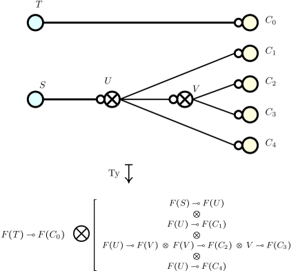
Figure 9. A transformation forest $\mathcal{F}:T\with S\to\displaystyle\bigwith_{i=0}^{4}C_{i}$  ($S,T,U,V,C_{0},\ldots,C_{4}\in\mathsf{Obj}(\mathcal{C})$).

To guide the intuition, one may note that there is an embedding of a set of suitable labellings of the forest $\mathcal{F}$ into $\mathsf{Hom}_{\mathcal{D}}\left(\top,\mathrm{Ty}(\mathcal{F})\right)$.

We will now call abusively the input of $\mathcal{F}$ the object $A=\bigwith_{i\in I}C_{i}$ and the output $B=\bigwith_{o\in O}C_{o}$; we write $\mathcal{F}:A\to B$ in the sequel. The justification for this notation is that there is a family of maps

$${\llbracket\mathcal{F}\rrbracket}\;\in\;\prod_{o\in O}\sum_{i\in I}\mathsf{Hom}_{\mathcal{D}}\left(\mathrm{Ty}(\mathcal{F}),F(C_{i})\multimap F(C_{o})\right)$$

obtained by internalizing the composition of morphisms along branches of $\mathcal{F}$, which we call the semantics of $\mathcal{F}$.

We also note that this allow to interpret arbitrary $\mathcal{C}_{\with}$ morphisms: such a morphism $f:A\to B$ can be mapped to a pair $(\mathrm{Grph}(f),\widehat{f})$ consisting of

• a depth-1 transformation forest $\mathrm{Grph}(f):\bigwith_{i\in I}C_{i}\to\bigwith_{o\in O}C_{o}$ (an example is depicted in Figure 10)

• a morphism $\widehat{f}\in\mathsf{Hom}_{\mathcal{D}}\left(\top,\mathrm{Ty}(\mathcal{F})\right)$

so that, if $f=(i_{o},\alpha_{o})_{o\in O}$, we have ${\llbracket\mathrm{Grph}(f)\rrbracket}_{o}\circ\widehat{f}=(i_{o},\Lambda(\alpha_{o}\circ\rho^{-1}))$.

 

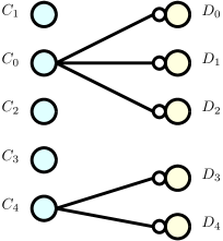
Figure 10. A depth-$1$ transformation forest.

Given two forests $\mathcal{F}:A\to B$ and $\mathcal{F}^{\prime}:B\to C$, there is a composition $\mathcal{F}^{\prime}\circ\mathcal{F}$ obtained by gluing the input nodes of $\mathcal{F}^{\prime}$ along the output nodes of $\mathcal{F}$. A crucial point is that the semantics of the composite ${\llbracket-\rrbracket}$ may be computed as follows

$${\llbracket\mathcal{F}^{\prime}\circ\mathcal{F}\rrbracket}(o)\;=\;\left({\llbracket\mathcal{F}\rrbracket}_{1}({\llbracket\mathcal{F}^{\prime}\rrbracket}_{1}(o^{\prime})),{\llbracket\mathcal{F}^{\prime}\rrbracket}_{2}(o^{\prime})\circ{\llbracket\mathcal{F}\rrbracket}_{2}({\llbracket\mathcal{F}^{\prime}\rrbracket}_{1})\right)$$

4.2.2. Reducing transformation forests

We now introduce two elementary transformations $\mathcal{F}\mapsto\mathcal{F}^{\prime}$ over transformation forests, together with associated morphisms $\mathrm{Ty}(\mathcal{F})\to\mathrm{Ty}(\mathcal{F}^{\prime})$:

• Pruning: if $v\in V_{\mathcal{F}}$ is a leaf which is not an output node in the forest $\mathcal{F}:A\to B$, call $\mathrm{prune}(\mathcal{F},v):A\to B$ the forest obtained by removing $v$ and adjacent edges from $\mathcal{F}$.

  This induces a canonical map

  $${prune}(v):\mathrm{Ty}(\mathcal{F})\to\mathrm{Ty}(\mathrm{prune}(\mathcal{F},v))$$

  by using the weakening maps on the components corresponding to the deleted edges.

• Contraction: If there is a vertex $v$ with a unique child $c$ and a (unique) parent $p$ in the forest $\mathcal{F}:A\to B$, call $\mathrm{contract}(\mathcal{F},v):A\to B$ the forest obtained by replacing the edges $(p,v)$ and $(v,c)$ with a single edge $(p,c)$ and removing $v$.

  There is a canonical map

  $${contract}(v):\mathrm{Ty}(\mathcal{F})\to\mathrm{Ty}(\mathrm{contract}(\mathcal{F},v))$$

  induced by the internal composition map

  $$\mathsf{Hom}_{\mathcal{D}}\left([F(C_{p})\multimap F(C_{v})]\otimes[F(C_{v})\multimap F(C_{c})],F(C_{p})\multimap F(C_{c})\right)$$

The auxiliary maps ${prune}$ and ${contract}$ operations are compatible with the semantic map ${\llbracket\cdot\rrbracket}$ in the sense that for every $o\in O$ and suitable vertices $u,v$ of $\mathcal{F}$ , we have

$$i=\pi_{1}({\llbracket\mathcal{F}\rrbracket}(o))=\pi_{1}({\llbracket\mathrm{prune}(\mathcal{F},u)\rrbracket}(o))=\pi_{1}({\llbracket\mathrm{contract}(\mathcal{F},v)\rrbracket}(o))$$

and the following diagrams commute in $\mathcal{D}$

Consider the rewrite system $\leadsto$ over forests $\mathcal{F}:A\to B$ induced by those two operations, and call $\leadsto^{=}$ its reflexive closure and $\leadsto^{*}$ the transitive closure of $\leadsto^{=}$. It can be shown that the reflexive closure $\leadsto^{=}$ satisfies the diamond lemma, i.e., that for every $\mathcal{F},\mathcal{F}^{\prime}$ and $\mathcal{F}^{\prime\prime}$ such that $\mathcal{F}\leadsto^{=}\mathcal{F}^{\prime}$ and $\mathcal{F}\leadsto^{=}\mathcal{F}^{\prime\prime}$, there exists $\mathcal{F}^{\prime\prime\prime}$ such that $\mathcal{F}^{\prime}\leadsto^{=}\mathcal{F}^{\prime\prime\prime}$ and $\mathcal{F}^{\prime\prime}\leadsto^{=}\mathcal{F}^{\prime\prime\prime}$. This ensures that $\leadsto$ is confluent. Furthermore, given a rewrite $\mathcal{F}\leadsto^{*}\mathcal{F}^{\prime}$, there is a map $\mathrm{Ty}(\mathcal{F})\to\mathrm{Ty}(\mathcal{F}^{\prime})$ obtained by composing maps ${prune}(v)$ and ${contract}(v)$ (and identities for trivial rewrites $\mathcal{F}\leadsto^{*}\mathcal{F}$). It can be shown that this map does not depend on the rewrite path. This is done first by arguing that if we have a rewrite square for $\leadsto^{=}$, the associated diagram in $\mathcal{D}$ is commutative, and then proceed by induction over the rewrite paths using the diamond lemma.

$$\lx@xy@svg{\hbox{\raise 0.0pt\hbox{\kern 7.8039pt\hbox{\ignorespaces\ignorespaces\ignorespaces\hbox{\vtop{\kern 0.0pt\offinterlineskip\halign{\entry@#!@&&\entry@@#!@\cr&\\&\\}}}\ignorespaces{\hbox{\kern-6.2639pt\raise 0.0pt\hbox{\hbox{\kern 0.0pt\raise 0.0pt\hbox{\hbox{\kern 3.0pt\raise 0.0pt\hbox{$\textstyle{\mathcal{F}\ignorespaces\ignorespaces\ignorespaces\ignorespaces\ignorespaces\ignorespaces\ignorespaces\ignorespaces}$}}}}}}}\ignorespaces\ignorespaces\ignorespaces{}\ignorespaces\ignorespaces{\hbox{\lx@xy@drawsquiggles@}}\ignorespaces{\hbox{\kern 66.24939pt\raise 0.0pt\hbox{\hbox{\kern 0.0pt\raise 0.0pt\hbox{\lx@xy@tip{1}\lx@xy@tip{-1}}}}}}\ignorespaces\ignorespaces{\hbox{\lx@xy@drawsquiggles@}}\ignorespaces{\hbox{\lx@xy@drawsquiggles@}}\ignorespaces\ignorespaces\ignorespaces{}\ignorespaces\ignorespaces{\hbox{\lx@xy@drawsquiggles@}}\ignorespaces{\hbox{\kern 0.0pt\raise-26.99998pt\hbox{\hbox{\kern 0.0pt\raise 0.0pt\hbox{\lx@xy@tip{1}\lx@xy@tip{-1}}}}}}\ignorespaces\ignorespaces{\hbox{\lx@xy@drawsquiggles@}}\ignorespaces{\hbox{\lx@xy@drawsquiggles@}}{\hbox{\kern 66.24939pt\raise 0.0pt\hbox{\hbox{\kern 0.0pt\raise 0.0pt\hbox{\hbox{\kern 3.0pt\raise 0.0pt\hbox{$\textstyle{\mathcal{F}^{\prime}\ignorespaces\ignorespaces\ignorespaces\ignorespaces}$}}}}}}}\ignorespaces\ignorespaces\ignorespaces{}\ignorespaces\ignorespaces{\hbox{\lx@xy@drawsquiggles@}}\ignorespaces{\hbox{\kern 73.28328pt\raise-26.99998pt\hbox{\hbox{\kern 0.0pt\raise 0.0pt\hbox{\lx@xy@tip{1}\lx@xy@tip{-1}}}}}}\ignorespaces\ignorespaces{\hbox{\lx@xy@drawsquiggles@}}\ignorespaces{\hbox{\lx@xy@drawsquiggles@}}{\hbox{\kern-7.8039pt\raise-38.38885pt\hbox{\hbox{\kern 0.0pt\raise 0.0pt\hbox{\hbox{\kern 3.0pt\raise 0.0pt\hbox{$\textstyle{\mathcal{F}^{\prime\prime}\ignorespaces\ignorespaces\ignorespaces\ignorespaces}$}}}}}}}\ignorespaces\ignorespaces\ignorespaces{}\ignorespaces\ignorespaces{\hbox{\lx@xy@drawsquiggles@}}\ignorespaces{\hbox{\kern 64.7094pt\raise-38.38885pt\hbox{\hbox{\kern 0.0pt\raise 0.0pt\hbox{\lx@xy@tip{1}\lx@xy@tip{-1}}}}}}\ignorespaces\ignorespaces{\hbox{\lx@xy@drawsquiggles@}}\ignorespaces{\hbox{\lx@xy@drawsquiggles@}}{\hbox{\kern 64.7094pt\raise-38.38885pt\hbox{\hbox{\kern 0.0pt\raise 0.0pt\hbox{\hbox{\kern 3.0pt\raise 0.0pt\hbox{$\textstyle{\mathcal{F}^{\prime\prime\prime}}$}}}}}}}\ignorespaces}}}}\ignorespaces\qquad\qquad\begin{array}[]{c}\\ \\ \\ \longmapsto\end{array}\qquad\qquad\lx@xy@svg{\hbox{\raise 0.0pt\hbox{\kern 17.80391pt\hbox{\ignorespaces\ignorespaces\ignorespaces\hbox{\vtop{\kern 0.0pt\offinterlineskip\halign{\entry@#!@&&\entry@@#!@\cr&\\&\\}}}\ignorespaces{\hbox{\kern-16.26392pt\raise 0.0pt\hbox{\hbox{\kern 0.0pt\raise 0.0pt\hbox{\hbox{\kern 3.0pt\raise 0.0pt\hbox{$\textstyle{\mathrm{Ty}(\mathcal{F})\ignorespaces\ignorespaces\ignorespaces\ignorespaces\ignorespaces\ignorespaces\ignorespaces\ignorespaces}$}}}}}}}\ignorespaces\ignorespaces\ignorespaces\ignorespaces{}{\hbox{\lx@xy@droprule}}\ignorespaces{\hbox{\kern 76.24939pt\raise 0.0pt\hbox{\hbox{\kern 0.0pt\raise 0.0pt\hbox{\lx@xy@tip{1}\lx@xy@tip{-1}}}}}}{\hbox{\lx@xy@droprule}}{\hbox{\lx@xy@droprule}}\ignorespaces\ignorespaces\ignorespaces\ignorespaces{}{\hbox{\lx@xy@droprule}}\ignorespaces{\hbox{\kern 0.0pt\raise-29.49998pt\hbox{\hbox{\kern 0.0pt\raise 0.0pt\hbox{\lx@xy@tip{1}\lx@xy@tip{-1}}}}}}{\hbox{\lx@xy@droprule}}{\hbox{\lx@xy@droprule}}{\hbox{\kern 76.24939pt\raise 0.0pt\hbox{\hbox{\kern 0.0pt\raise 0.0pt\hbox{\hbox{\kern 3.0pt\raise 0.0pt\hbox{$\textstyle{\mathrm{Ty}(\mathcal{F}^{\prime})\ignorespaces\ignorespaces\ignorespaces\ignorespaces}$}}}}}}}\ignorespaces\ignorespaces\ignorespaces\ignorespaces{}{\hbox{\lx@xy@droprule}}\ignorespaces{\hbox{\kern 93.28331pt\raise-29.49998pt\hbox{\hbox{\kern 0.0pt\raise 0.0pt\hbox{\lx@xy@tip{1}\lx@xy@tip{-1}}}}}}{\hbox{\lx@xy@droprule}}{\hbox{\lx@xy@droprule}}{\hbox{\kern-17.80391pt\raise-40.88885pt\hbox{\hbox{\kern 0.0pt\raise 0.0pt\hbox{\hbox{\kern 3.0pt\raise 0.0pt\hbox{$\textstyle{\mathrm{Ty}(\mathcal{F}^{\prime\prime})\ignorespaces\ignorespaces\ignorespaces\ignorespaces}$}}}}}}}\ignorespaces\ignorespaces\ignorespaces\ignorespaces{}{\hbox{\lx@xy@droprule}}\ignorespaces{\hbox{\kern 74.70941pt\raise-40.88885pt\hbox{\hbox{\kern 0.0pt\raise 0.0pt\hbox{\lx@xy@tip{1}\lx@xy@tip{-1}}}}}}{\hbox{\lx@xy@droprule}}{\hbox{\lx@xy@droprule}}{\hbox{\kern 74.70941pt\raise-40.88885pt\hbox{\hbox{\kern 0.0pt\raise 0.0pt\hbox{\hbox{\kern 3.0pt\raise 0.0pt\hbox{$\textstyle{\mathrm{Ty}(\mathcal{F}^{\prime\prime\prime})}$}}}}}}}\ignorespaces}}}}\ignorespaces \textstyle{\mathcal{F}\ignorespaces\ignorespaces\ignorespaces\ignorespaces\ignorespaces\ignorespaces\ignorespaces\ignorespaces} \textstyle{\mathcal{F}^{\prime}\ignorespaces\ignorespaces\ignorespaces\ignorespaces} \textstyle{\mathcal{F}^{\prime\prime}\ignorespaces\ignorespaces\ignorespaces\ignorespaces} \textstyle{\mathcal{F}^{\prime\prime\prime}} \textstyle{\mathrm{Ty}(\mathcal{F})\ignorespaces\ignorespaces\ignorespaces\ignorespaces\ignorespaces\ignorespaces\ignorespaces\ignorespaces} \textstyle{\mathrm{Ty}(\mathcal{F}^{\prime})\ignorespaces\ignorespaces\ignorespaces\ignorespaces} \textstyle{\mathrm{Ty}(\mathcal{F}^{\prime\prime})\ignorespaces\ignorespaces\ignorespaces\ignorespaces} \textstyle{\mathrm{Ty}(\mathcal{F}^{\prime\prime\prime})} \textstyle{\mathcal{F}\ignorespaces\ignorespaces\ignorespaces\ignorespaces\ignorespaces\ignorespaces\ignorespaces\ignorespaces} \textstyle{\mathcal{F}^{\prime}\ignorespaces\ignorespaces\ignorespaces\ignorespaces} \textstyle{\mathcal{F}^{\prime\prime}\ignorespaces\ignorespaces\ignorespaces\ignorespaces} \textstyle{\mathcal{F}^{\prime\prime\prime}} \textstyle{\mathrm{Ty}(\mathcal{F})\ignorespaces\ignorespaces\ignorespaces\ignorespaces\ignorespaces\ignorespaces\ignorespaces\ignorespaces} \textstyle{\mathrm{Ty}(\mathcal{F}^{\prime})\ignorespaces\ignorespaces\ignorespaces\ignorespaces} \textstyle{\mathrm{Ty}(\mathcal{F}^{\prime\prime})\ignorespaces\ignorespaces\ignorespaces\ignorespaces} \textstyle{\mathrm{Ty}(\mathcal{F}^{\prime\prime\prime})}$$

Defining the size of a forest as its number of vertices, it is clear that $\mathrm{prune}(\mathcal{F},u)$ and $\mathrm{contract}(\mathcal{F},v)$ have size strictly less than $\mathcal{F}$, so the rewrite system is also terminating. With confluence, it means that for every forest $\mathcal{F}:A\to B$, there is a unique forest $\mathrm{reduce}(\mathcal{F}):A\to B$ such that $\mathcal{F}\leadsto^{*}\mathrm{reduce}(\mathcal{F})$ and there is no $\mathcal{F}^{\prime}$ such that $\mathrm{reduce}(\mathcal{F})\leadsto\mathcal{F}^{\prime}$. We call $\mathrm{reduce}(\mathcal{F})$ the normal form of $\mathcal{F}$; a forest $\mathcal{F}$ is called normal if $\mathrm{reduce}(\mathcal{F})=\mathcal{F}$. By the discussion above, there are canonical maps $reduce_{\mathcal{F}}:\mathrm{Ty}(\mathcal{F})\to\mathrm{Ty}(\mathrm{reduce}(\mathcal{F}))$ coming from rewrites.

 

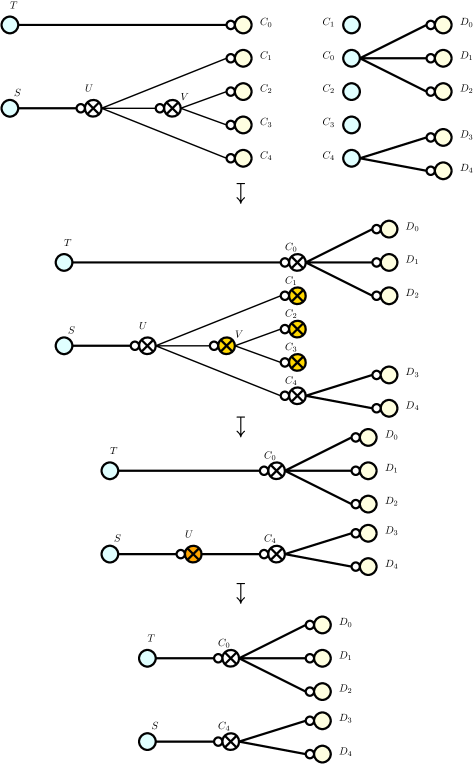
Figure 11. An example of composing normal transformation forests, where first the usual composition and then two big steps of reduction, corresponding respectively to pruning and contracting, are carried out in succession.

The last important thing to note is that, if the input $A=\bigwith_{i\in I}C_{i}$ and output $B=\bigwith_{o\in O}C_{o}$ are fixed, up to isomorphism, there are finitely many normal forests $\mathcal{F}:A\to B$ as their size is bounded by $2({|I|}+{|O|})$. We write $\mathrm{NF}\left({A},{B}\right)$ for a finite set of representative for all normal forests $A\to B$, and given $\mathcal{F}\in\mathrm{NF}\left({B},{C}\right)$ and $\mathcal{F}^{\prime}\in\mathrm{NF}\left({A},{B}\right)$, we write $\mathcal{F}\circ_{\mathcal{N}}\mathcal{F}^{\prime}$ for the unique forest in $\mathrm{NF}\left({A},{C}\right)$ which is isomorphic to $\mathrm{reduce}(\mathcal{F}\circ\mathcal{F}^{\prime})$; an example of the full computation of a $\mathcal{F}\circ_{\mathcal{N}}\mathcal{F}^{\prime}$ is given in Figure 11. Similarly, we assume that $\mathrm{Grph}(f)\in\mathrm{NF}\left({A},{B}\right)$ for every morphism $f\in\mathsf{Hom}_{\mathcal{C}_{\with}}\left(A,B\right)$.

4.2.3. Putting everything together

Let $\mathcal{T}=\left(Q,q_{0},\left(A_{q}\right)_{q\in Q},\delta,i,o\right)$ be a sdm-$\mathfrak{C}_{\with}$-SST with input $\Sigma^{*}$. We define the sdm-$\mathfrak{D}$-SST

$$\mathcal{T}^{\prime}\leavevmode\nobreak\ \leavevmode\nobreak\ =\leavevmode\nobreak\ \leavevmode\nobreak\ \left(\sum_{q\in Q}\mathrm{NF}\left({A_{q_{0}}},{A_{q}}\right),(q_{0},\mathrm{Grph}(\mathrm{id})),(\mathrm{Ty}(\mathcal{F}))_{q,\mathcal{F}},\delta^{\prime},i^{\prime}o^{\prime}\right)$$

where

$$\begin{array}[]{c}\displaystyle\delta^{\prime}\leavevmode\nobreak\ \leavevmode\nobreak\ :\leavevmode\nobreak\ \leavevmode\nobreak\ \Sigma\to\prod_{q,\mathcal{F}}\sum_{r,\mathcal{F}^{\prime}}\mathsf{Hom}_{\mathcal{D}}\left(\mathrm{Ty}(\mathcal{F}),\mathrm{Ty}(\mathcal{F}^{\prime})\right)\\ \\ \displaystyle i^{\prime}\in\mathsf{Hom}_{\mathcal{D}}\left(\text{{\raisebox{0.0pt}{\scalebox{1.0}[-1.0]{$\Bot$}}}},\mathrm{Grph}(\mathrm{id})\right)\qquad\qquad o^{\prime}\in\prod_{q,\mathcal{F}}\mathsf{Hom}_{\mathcal{D}}\left(\mathrm{Ty}(\mathcal{F}),\Bot\right)\end{array}$$

are given as follows, assuming that $A_{q}=\displaystyle\bigwith_{x\in X_{q}}C_{q,x}$

$$\begin{array}[]{|c@{\qquad}|@{\qquad}c|}\hline\cr\delta^{\mathcal{D}}(a)_{q,\mathcal{F}}&o^{\prime}_{q,\mathcal{F}}\\ \hline\cr&\\ \lx@xy@svg{\hbox{\raise 0.0pt\hbox{\kern 66.84872pt\hbox{\ignorespaces\ignorespaces\ignorespaces\hbox{\vtop{\kern 0.0pt\offinterlineskip\halign{\entry@#!@&&\entry@@#!@\cr\\\\\\\\\\\\\\}}}\ignorespaces{\hbox{\kern-3.0pt\raise 0.0pt\hbox{\hbox{\kern 0.0pt\raise 0.0pt\hbox{\hbox{\kern 3.0pt\raise 0.0pt\hbox{$\textstyle{}$}}}}}}}{\hbox{\kern-16.26392pt\raise-35.0pt\hbox{\hbox{\kern 0.0pt\raise 0.0pt\hbox{\hbox{\kern 3.0pt\raise 0.0pt\hbox{$\textstyle{\mathrm{Ty}(\mathcal{F})\ignorespaces\ignorespaces\ignorespaces\ignorespaces}$}}}}}}}\ignorespaces\ignorespaces\ignorespaces\ignorespaces{}{\hbox{\lx@xy@droprule}}\ignorespaces\ignorespaces\ignorespaces{\hbox{\kern 0.0pt\raise-55.0pt\hbox{{}\hbox{\kern 0.0pt\raise 0.0pt\hbox{\hbox{\kern 3.0pt\hbox{\hbox{\kern 0.0pt\raise-1.28406pt\hbox{$\scriptstyle{\sim}$}}}\kern 3.0pt}}}}}}\ignorespaces{\hbox{\kern 0.0pt\raise-64.5pt\hbox{\hbox{\kern 0.0pt\raise 0.0pt\hbox{\lx@xy@tip{1}\lx@xy@tip{-1}}}}}}{\hbox{\lx@xy@droprule}}{\hbox{\lx@xy@droprule}}{\hbox{\kern-24.04172pt\raise-75.0pt\hbox{\hbox{\kern 0.0pt\raise 0.0pt\hbox{\hbox{\kern 3.0pt\raise 0.0pt\hbox{$\textstyle{\top\otimes\mathrm{Ty}(\mathcal{F})\ignorespaces\ignorespaces\ignorespaces\ignorespaces}$}}}}}}}\ignorespaces\ignorespaces\ignorespaces\ignorespaces{}{\hbox{\lx@xy@droprule}}\ignorespaces\ignorespaces\ignorespaces{\hbox{\kern 0.0pt\raise-95.33943pt\hbox{{}\hbox{\kern 0.0pt\raise 0.0pt\hbox{\hbox{\kern 3.0pt\hbox{\hbox{\kern 0.0pt\raise-3.31946pt\hbox{$\scriptstyle{\widehat{\delta^{\mathcal{C}_{\with}}(a)_{q}}\otimes\mathrm{id}}$}}}\kern 3.0pt}}}}}}\ignorespaces{\hbox{\kern 0.0pt\raise-103.8211pt\hbox{\hbox{\kern 0.0pt\raise 0.0pt\hbox{\lx@xy@tip{1}\lx@xy@tip{-1}}}}}}{\hbox{\lx@xy@droprule}}{\hbox{\lx@xy@droprule}}{\hbox{\kern-60.16817pt\raise-115.67888pt\hbox{\hbox{\kern 0.0pt\raise 0.0pt\hbox{\hbox{\kern 3.0pt\raise 0.0pt\hbox{$\textstyle{\mathrm{Ty}(\mathrm{Grph}(\delta^{\mathcal{C}_{\with}}(a)_{q}))\otimes\mathrm{Ty}(\mathcal{F})\ignorespaces\ignorespaces\ignorespaces\ignorespaces}$}}}}}}}\ignorespaces\ignorespaces\ignorespaces\ignorespaces{}{\hbox{\lx@xy@droprule}}\ignorespaces\ignorespaces\ignorespaces{\hbox{\kern 0.0pt\raise-136.35776pt\hbox{{}\hbox{\kern 0.0pt\raise 0.0pt\hbox{\hbox{\kern 3.0pt\hbox{\hbox{\kern 0.0pt\raise-1.28406pt\hbox{$\scriptstyle{\sim}$}}}\kern 3.0pt}}}}}}\ignorespaces{\hbox{\kern 0.0pt\raise-145.17886pt\hbox{\hbox{\kern 0.0pt\raise 0.0pt\hbox{\lx@xy@tip{1}\lx@xy@tip{-1}}}}}}{\hbox{\lx@xy@droprule}}{\hbox{\lx@xy@droprule}}{\hbox{\kern-48.77925pt\raise-157.03664pt\hbox{\hbox{\kern 0.0pt\raise 0.0pt\hbox{\hbox{\kern 3.0pt\raise 0.0pt\hbox{$\textstyle{\mathrm{Ty}(\mathrm{Grph}(\delta^{\mathcal{C}_{\with}}(a)_{q})\circ\mathcal{F})\ignorespaces\ignorespaces\ignorespaces\ignorespaces}$}}}}}}}\ignorespaces\ignorespaces\ignorespaces\ignorespaces{}{\hbox{\lx@xy@droprule}}\ignorespaces\ignorespaces\ignorespaces{\hbox{\kern 0.0pt\raise-177.71552pt\hbox{{}\hbox{\kern 0.0pt\raise 0.0pt\hbox{\hbox{\kern 3.0pt\hbox{\hbox{\kern 0.0pt\raise-2.43056pt\hbox{$\scriptstyle{reduce}$}}}\kern 3.0pt}}}}}}\ignorespaces{\hbox{\kern 0.0pt\raise-186.53662pt\hbox{\hbox{\kern 0.0pt\raise 0.0pt\hbox{\lx@xy@tip{1}\lx@xy@tip{-1}}}}}}{\hbox{\lx@xy@droprule}}{\hbox{\lx@xy@droprule}}{\hbox{\kern-66.84872pt\raise-198.3944pt\hbox{\hbox{\kern 0.0pt\raise 0.0pt\hbox{\hbox{\kern 3.0pt\raise 0.0pt\hbox{$\textstyle{\mathrm{Ty}(\mathrm{reduce}(\mathrm{Grph}(\delta^{\mathcal{C}_{\with}}(a)_{q})\circ\mathcal{F}))\ignorespaces\ignorespaces\ignorespaces\ignorespaces}$}}}}}}}\ignorespaces\ignorespaces\ignorespaces\ignorespaces{}{\hbox{\hbox{\kern 1.0pt\raise 0.0pt\hbox{\lx@xy@droprule}}\hbox{\kern-1.0pt\raise 0.0pt\hbox{\lx@xy@droprule}}}}\ignorespaces{}{\hbox{\hbox{\kern 1.0pt\raise 0.0pt\hbox{\lx@xy@droprule}}\hbox{\kern-1.0pt\raise 0.0pt\hbox{\lx@xy@droprule}}}}{\hbox{\hbox{\kern 1.0pt\raise 0.0pt\hbox{\lx@xy@droprule}}\hbox{\kern-1.0pt\raise 0.0pt\hbox{\lx@xy@droprule}}}}{\hbox{\kern-29.63785pt\raise-240.00327pt\hbox{\hbox{\kern 0.0pt\raise 0.0pt\hbox{\hbox{\kern 3.0pt\raise 0.0pt\hbox{$\textstyle{\mathrm{Ty}(\delta^{\mathrm{NF}}(a)_{q,\mathcal{F}})}$}}}}}}}\ignorespaces}}}}\ignorespaces&\lx@xy@svg{\hbox{\raise 0.0pt\hbox{\kern 70.90828pt\hbox{\ignorespaces\ignorespaces\ignorespaces\hbox{\vtop{\kern 0.0pt\offinterlineskip\halign{\entry@#!@&&\entry@@#!@\cr\\\\\\\\\\\\\\\crcr}}}\ignorespaces{\hbox{\kern-16.26392pt\raise 0.0pt\hbox{\hbox{\kern 0.0pt\raise 0.0pt\hbox{\hbox{\kern 3.0pt\raise 0.0pt\hbox{$\textstyle{\mathrm{Ty}(\mathcal{F})\ignorespaces\ignorespaces\ignorespaces\ignorespaces}$}}}}}}}\ignorespaces\ignorespaces\ignorespaces\ignorespaces{}{\hbox{\lx@xy@droprule}}\ignorespaces\ignorespaces\ignorespaces{\hbox{\kern 0.0pt\raise-20.0pt\hbox{{}\hbox{\kern 0.0pt\raise 0.0pt\hbox{\hbox{\kern 3.0pt\hbox{\hbox{\kern 0.0pt\raise-1.75pt\hbox{$\scriptstyle{f}$}}}\kern 3.0pt}}}}}}\ignorespaces{\hbox{\kern 0.0pt\raise-29.5pt\hbox{\hbox{\kern 0.0pt\raise 0.0pt\hbox{\lx@xy@tip{1}\lx@xy@tip{-1}}}}}}{\hbox{\lx@xy@droprule}}{\hbox{\lx@xy@droprule}}{\hbox{\kern-43.84996pt\raise-40.0pt\hbox{\hbox{\kern 0.0pt\raise 0.0pt\hbox{\hbox{\kern 3.0pt\raise 0.0pt\hbox{$\textstyle{{F(C_{q_{0},x_{0}})}\multimap{F(C_{q,x})}\ignorespaces\ignorespaces\ignorespaces\ignorespaces}$}}}}}}}\ignorespaces\ignorespaces\ignorespaces\ignorespaces{}{\hbox{\lx@xy@droprule}}\ignorespaces\ignorespaces\ignorespaces{\hbox{\kern 0.0pt\raise-60.0pt\hbox{{}\hbox{\kern 0.0pt\raise 0.0pt\hbox{\hbox{\kern 3.0pt\hbox{\hbox{\kern 0.0pt\raise-1.28406pt\hbox{$\scriptstyle{\sim}$}}}\kern 3.0pt}}}}}}\ignorespaces{\hbox{\kern 0.0pt\raise-69.5pt\hbox{\hbox{\kern 0.0pt\raise 0.0pt\hbox{\lx@xy@tip{1}\lx@xy@tip{-1}}}}}}{\hbox{\lx@xy@droprule}}{\hbox{\lx@xy@droprule}}{\hbox{\kern-57.27356pt\raise-80.0pt\hbox{\hbox{\kern 0.0pt\raise 0.0pt\hbox{\hbox{\kern 3.0pt\raise 0.0pt\hbox{$\textstyle{({F(C_{q_{0},x_{0}})}\multimap{F(C_{q,x})})\otimes\text{{\raisebox{0.0pt}{\scalebox{1.0}[-1.0]{$\Bot$}}}}\ignorespaces\ignorespaces\ignorespaces\ignorespaces}$}}}}}}}\ignorespaces\ignorespaces\ignorespaces\ignorespaces{}{\hbox{\lx@xy@droprule}}\ignorespaces{\hbox{\kern 0.0pt\raise-109.5pt\hbox{\hbox{\kern 0.0pt\raise 0.0pt\hbox{\lx@xy@tip{1}\lx@xy@tip{-1}}}}}}{\hbox{\lx@xy@droprule}}{\hbox{\lx@xy@droprule}}{\hbox{\kern-66.18327pt\raise-120.0pt\hbox{\hbox{\kern 0.0pt\raise 0.0pt\hbox{\hbox{\kern 3.0pt\raise 0.0pt\hbox{$\textstyle{({F(C_{q_{0},x_{0}})}\multimap{F(C_{q,x})})\otimes F(\text{{\raisebox{0.0pt}{\scalebox{1.0}[-1.0]{$\Bot$}}}})\ignorespaces\ignorespaces\ignorespaces\ignorespaces}$}}}}}}}\ignorespaces\ignorespaces\ignorespaces\ignorespaces{}{\hbox{\lx@xy@droprule}}\ignorespaces\ignorespaces\ignorespaces{\hbox{\kern 0.0pt\raise-140.0pt\hbox{{}\hbox{\kern 0.0pt\raise 0.0pt\hbox{\hbox{\kern 3.0pt\hbox{\hbox{\kern 0.0pt\raise-1.6789pt\hbox{$\scriptstyle{\mathrm{id}\otimes F(i_{x_{0}})}$}}}\kern 3.0pt}}}}}}\ignorespaces{\hbox{\kern 0.0pt\raise-149.5pt\hbox{\hbox{\kern 0.0pt\raise 0.0pt\hbox{\lx@xy@tip{1}\lx@xy@tip{-1}}}}}}{\hbox{\lx@xy@droprule}}{\hbox{\lx@xy@droprule}}{\hbox{\kern-70.90828pt\raise-160.0pt\hbox{\hbox{\kern 0.0pt\raise 0.0pt\hbox{\hbox{\kern 3.0pt\raise 0.0pt\hbox{$\textstyle{({F(C_{q_{0},x_{0}})}\multimap{F(C_{q,x})})\otimes F(C_{q_{0},x_{0}})\ignorespaces\ignorespaces\ignorespaces\ignorespaces}$}}}}}}}\ignorespaces\ignorespaces\ignorespaces\ignorespaces{}{\hbox{\lx@xy@droprule}}\ignorespaces\ignorespaces\ignorespaces{\hbox{\kern 0.0pt\raise-180.0pt\hbox{{}\hbox{\kern 0.0pt\raise 0.0pt\hbox{\hbox{\kern 3.0pt\hbox{\hbox{\kern 0.0pt\raise-1.50694pt\hbox{$\scriptstyle{\mathrm{ev}}$}}}\kern 3.0pt}}}}}}\ignorespaces{\hbox{\kern 0.0pt\raise-189.5pt\hbox{\hbox{\kern 0.0pt\raise 0.0pt\hbox{\lx@xy@tip{1}\lx@xy@tip{-1}}}}}}{\hbox{\lx@xy@droprule}}{\hbox{\lx@xy@droprule}}{\hbox{\kern-18.45834pt\raise-200.0pt\hbox{\hbox{\kern 0.0pt\raise 0.0pt\hbox{\hbox{\kern 3.0pt\raise 0.0pt\hbox{$\textstyle{F(C_{q,x})\ignorespaces\ignorespaces\ignorespaces\ignorespaces}$}}}}}}}\ignorespaces\ignorespaces\ignorespaces\ignorespaces{}{\hbox{\lx@xy@droprule}}\ignorespaces\ignorespaces\ignorespaces{\hbox{\kern 0.0pt\raise-220.0pt\hbox{{}\hbox{\kern 0.0pt\raise 0.0pt\hbox{\hbox{\kern 3.0pt\hbox{\hbox{\kern 0.0pt\raise-1.75pt\hbox{$\scriptstyle{F(o^{\mathcal{C}})}$}}}\kern 3.0pt}}}}}}\ignorespaces{\hbox{\kern 0.0pt\raise-229.5pt\hbox{\hbox{\kern 0.0pt\raise 0.0pt\hbox{\lx@xy@tip{1}\lx@xy@tip{-1}}}}}}{\hbox{\lx@xy@droprule}}{\hbox{\lx@xy@droprule}}{\hbox{\kern-15.33334pt\raise-240.0pt\hbox{\hbox{\kern 0.0pt\raise 0.0pt\hbox{\hbox{\kern 3.0pt\raise 0.0pt\hbox{$\textstyle{F(\Bot)\ignorespaces\ignorespaces\ignorespaces\ignorespaces}$}}}}}}}\ignorespaces\ignorespaces\ignorespaces\ignorespaces{}{\hbox{\lx@xy@droprule}}\ignorespaces{\hbox{\kern 0.0pt\raise-268.58334pt\hbox{\hbox{\kern 0.0pt\raise 0.0pt\hbox{\lx@xy@tip{1}\lx@xy@tip{-1}}}}}}{\hbox{\lx@xy@droprule}}{\hbox{\lx@xy@droprule}}{\hbox{\kern-7.53471pt\raise-278.41666pt\hbox{\hbox{\kern 0.0pt\raise 0.0pt\hbox{\hbox{\kern 3.0pt\raise 0.0pt\hbox{$\textstyle{\Bot}$}}}}}}}\ignorespaces}}}}\ignorespaces\\ \hline\cr\end{array} \textstyle{\mathrm{Ty}(\mathcal{F})\ignorespaces\ignorespaces\ignorespaces\ignorespaces} \scriptstyle{\sim} \textstyle{\top\otimes\mathrm{Ty}(\mathcal{F})\ignorespaces\ignorespaces\ignorespaces\ignorespaces} \scriptstyle{\widehat{\delta^{\mathcal{C}_{\with}}(a)_{q}}\otimes\mathrm{id}} \textstyle{\mathrm{Ty}(\mathrm{Grph}(\delta^{\mathcal{C}_{\with}}(a)_{q}))\otimes\mathrm{Ty}(\mathcal{F})\ignorespaces\ignorespaces\ignorespaces\ignorespaces} \scriptstyle{\sim} \textstyle{\mathrm{Ty}(\mathrm{Grph}(\delta^{\mathcal{C}_{\with}}(a)_{q})\circ\mathcal{F})\ignorespaces\ignorespaces\ignorespaces\ignorespaces} \scriptstyle{reduce} \textstyle{\mathrm{Ty}(\mathrm{reduce}(\mathrm{Grph}(\delta^{\mathcal{C}_{\with}}(a)_{q})\circ\mathcal{F}))\ignorespaces\ignorespaces\ignorespaces\ignorespaces} \textstyle{\mathrm{Ty}(\delta^{\mathrm{NF}}(a)_{q,\mathcal{F}})} \textstyle{\mathrm{Ty}(\mathcal{F})\ignorespaces\ignorespaces\ignorespaces\ignorespaces} \scriptstyle{f} \textstyle{{F(C_{q_{0},x_{0}})}\multimap{F(C_{q,x})}\ignorespaces\ignorespaces\ignorespaces\ignorespaces} \scriptstyle{\sim} \textstyle{({F(C_{q_{0},x_{0}})}\multimap{F(C_{q,x})})\otimes\text{{\raisebox{0.0pt}{\scalebox{1.0}[-1.0]{$\Bot$}}}}\ignorespaces\ignorespaces\ignorespaces\ignorespaces} \textstyle{({F(C_{q_{0},x_{0}})}\multimap{F(C_{q,x})})\otimes F(\text{{\raisebox{0.0pt}{\scalebox{1.0}[-1.0]{$\Bot$}}}})\ignorespaces\ignorespaces\ignorespaces\ignorespaces} \scriptstyle{\mathrm{id}\otimes F(i_{x_{0}})} \textstyle{({F(C_{q_{0},x_{0}})}\multimap{F(C_{q,x})})\otimes F(C_{q_{0},x_{0}})\ignorespaces\ignorespaces\ignorespaces\ignorespaces} \scriptstyle{\mathrm{ev}} \textstyle{F(C_{q,x})\ignorespaces\ignorespaces\ignorespaces\ignorespaces} \scriptstyle{F(o^{\mathcal{C}})} \textstyle{F(\Bot)\ignorespaces\ignorespaces\ignorespaces\ignorespaces} \textstyle{\Bot} \textstyle{\mathrm{Ty}(\mathcal{F})\ignorespaces\ignorespaces\ignorespaces\ignorespaces} \scriptstyle{\sim} \textstyle{\top\otimes\mathrm{Ty}(\mathcal{F})\ignorespaces\ignorespaces\ignorespaces\ignorespaces} \scriptstyle{\widehat{\delta^{\mathcal{C}_{\with}}(a)_{q}}\otimes\mathrm{id}} \textstyle{\mathrm{Ty}(\mathrm{Grph}(\delta^{\mathcal{C}_{\with}}(a)_{q}))\otimes\mathrm{Ty}(\mathcal{F})\ignorespaces\ignorespaces\ignorespaces\ignorespaces} \scriptstyle{\sim} \textstyle{\mathrm{Ty}(\mathrm{Grph}(\delta^{\mathcal{C}_{\with}}(a)_{q})\circ\mathcal{F})\ignorespaces\ignorespaces\ignorespaces\ignorespaces} \scriptstyle{reduce} \textstyle{\mathrm{Ty}(\mathrm{reduce}(\mathrm{Grph}(\delta^{\mathcal{C}_{\with}}(a)_{q})\circ\mathcal{F}))\ignorespaces\ignorespaces\ignorespaces\ignorespaces} \textstyle{\mathrm{Ty}(\delta^{\mathrm{NF}}(a)_{q,\mathcal{F}})} \textstyle{\mathrm{Ty}(\mathcal{F})\ignorespaces\ignorespaces\ignorespaces\ignorespaces} \scriptstyle{f} \textstyle{{F(C_{q_{0},x_{0}})}\multimap{F(C_{q,x})}\ignorespaces\ignorespaces\ignorespaces\ignorespaces} \scriptstyle{\sim} \textstyle{({F(C_{q_{0},x_{0}})}\multimap{F(C_{q,x})})\otimes\text{{\raisebox{0.0pt}{\scalebox{1.0}[-1.0]{$\Bot$}}}}\ignorespaces\ignorespaces\ignorespaces\ignorespaces} \textstyle{({F(C_{q_{0},x_{0}})}\multimap{F(C_{q,x})})\otimes F(\text{{\raisebox{0.0pt}{\scalebox{1.0}[-1.0]{$\Bot$}}}})\ignorespaces\ignorespaces\ignorespaces\ignorespaces} \scriptstyle{\mathrm{id}\otimes F(i_{x_{0}})} \textstyle{({F(C_{q_{0},x_{0}})}\multimap{F(C_{q,x})})\otimes F(C_{q_{0},x_{0}})\ignorespaces\ignorespaces\ignorespaces\ignorespaces} \scriptstyle{\mathrm{ev}} \textstyle{F(C_{q,x})\ignorespaces\ignorespaces\ignorespaces\ignorespaces} \scriptstyle{F(o^{\mathcal{C}})} \textstyle{F(\Bot)\ignorespaces\ignorespaces\ignorespaces\ignorespaces} \textstyle{\Bot}$$

Figure 12. Definition of $\delta^{\mathcal{D}}(a)_{q,\mathcal{F}}$ and $o^{\prime}_{q,\mathcal{F}}$.

• Notice that $\mathrm{Ty}(\mathrm{Grph}(\mathrm{id}))=\bigotimes_{x\in X_{q_{0}}}F(C_{q_{0},x})\multimap F(C_{q_{0},x})$; we simply take the constant map corresponding to the $X_{q_{0}}$-fold tensor of $\Lambda(\mathrm{id}_{C_{q_{0},x}})$ for $i^{\prime}$.

• Fix $a\in\Sigma$ and recall that $\delta(a)$ is a family of pairs

  $$(\delta^{Q}(a)_{q},\delta^{\mathcal{C}_{\with}}(a)_{q})_{q\in Q}\leavevmode\nobreak\ \leavevmode\nobreak\ \in\leavevmode\nobreak\ \leavevmode\nobreak\ \prod_{q\in Q}\sum_{r\in Q}\mathsf{Hom}_{\mathcal{C}_{\with}}\left(A_{q},A_{r}\right)$$

  $\delta^{\prime}$ is then defined by the equation

  $$\delta^{\prime}(a)_{q,\mathcal{F}}\leavevmode\nobreak\ \leavevmode\nobreak\ =\leavevmode\nobreak\ \leavevmode\nobreak\ \left(\left(\delta^{Q}(a)_{q},\delta^{\mathrm{NF}}(a)_{q,\mathcal{F}}\right),\delta^{\mathcal{D}}(a)_{q,\mathcal{F}}\right)$$

  where we set $\delta^{\mathrm{NF}}(a)_{q,\mathcal{F}}=\mathrm{Grph}(\delta^{\mathcal{C}_{\with}}(a)_{q})\circ_{\mathcal{N}}\mathcal{F}$ and $\delta^{\mathcal{D}}(a)_{q,\mathcal{F}}$ is obtained as in Figure 12

• Finally, for $q,\mathcal{F}$ ranging over states of $\mathcal{T}^{\prime}$, we define $o^{\prime}_{q,\mathcal{F}}$. Recall that $\mathcal{F}$ determines a canonical family

  $${\llbracket\mathcal{F}\rrbracket}\in\prod_{x\in X_{q}}\sum_{x_{0}\in X_{q_{0}}}\mathsf{Hom}_{\mathcal{D}}\left(\mathrm{Ty}(\mathcal{F}),F(C_{q_{0},x_{0}})\multimap F(C_{q,x})\right)$$

  First, as $\Bot^{\mathfrak{C}_{\with}}=\iota_{\with}(\Bot^{\mathfrak{C}})$, note that there is a unique $x\in X_{q}$ such that $o_{q}=(x,o^{\mathcal{C}})_{*}$ for some $o^{\mathcal{C}}\in\mathsf{Hom}_{\mathcal{C}}\left(C_{q,x},\Bot^{\mathfrak{C}}\right)$. Writing the pair ${\llbracket\mathcal{F}\rrbracket}_{x}$ as $(x_{0},f)$, $o^{\prime}_{q,\mathcal{F}}$ is depicted in Figure 12.

We omit the proof that ${\llbracket\mathcal{T}\rrbracket}={\llbracket\mathcal{T}^{\prime}\rrbracket}$ by induction over the length of an input word. While spelling it out may be a bit notation-heavy, there is no particular difficulty considering the remarks above linking ${\llbracket-\rrbracket}$, the composition of transformation forests and their normal forms.

5. Regular tree functions in the $\lambda\ell^{\oplus\with}$-calculus

The goal of this section is now to prove our main theorem for tree functions (that we recall below), extending the case of strings (Theorem 1).

See 2

To prove this theorem, we follow a similar approach as in Section 3.

Remark 52.

While the result on strings follows as a corollary of Theorem 2, this relies on the equivalence between regular string functions and regular tree functions when strings are regarded as particular trees. Given that we start from transducer-based characterization of these notions, this means that we would use e.g. [AD17, Theorem 3.16-3.17], which are themselves non-trivial results.

We thus first define a generalized notion of bottom-up ranked tree transducers (BRTT) parameterized by a notion of tree streaming setting.

Let $X$ be a set. A tree streaming setting with output $X$ is a tuple $\mathfrak{C}=(\mathcal{C},\otimes,\mathbf{I},\Bot,{\llparenthesis-\rrparenthesis})$ where

• $(\mathcal{C},\otimes,\mathbf{I})$ is a symmetric monoidal category

• $\Bot$ is an object of $\mathcal{C}$

• ${\llparenthesis-\rrparenthesis}$ is a set-theoretic map $\mathsf{Hom}_{\mathcal{C}}\left(\mathbf{I},\Bot\right)\to X$

This notion essentially differs by asking that the underlying category be equipped with a symmetric monoidal product, which is used in defining the semantics of $\mathfrak{C}$-BRTTs. The tensor product is used to fit the branching structure of trees and $\mathbf{I}$ is used for terminal nodes (so there is no need of a distinguished initial object $\Bot$ as in string streaming settings).

Let $\mathfrak{C}=(\mathcal{C},\otimes,\mathbf{I},\Bot,{\llparenthesis-\rrparenthesis})$ be a tree streaming setting with output $X$. A $\mathfrak{C}$-BRTT with input (ranked) alphabet $\bf\Sigma$ and output $X$ is a tuple $(Q,R,\delta,o)$ where

• $Q$ is a finite set of states

• $R$ is an object of $\mathcal{C}$

• $\delta$ is a function $\displaystyle\prod_{a\in\Sigma}\left(Q^{\mathrm{ar}(a)}\to Q\times\mathsf{Hom}_{\mathcal{C}}\left(\bigotimes_{\mathrm{ar}(a)}R\text{{\Huge{,}}}\;R\right)\right)$

• $o\in\mathsf{Hom}_{\mathcal{C}}\left(R,\Bot\right)$ is an output morphism

Its semantics is a set-theoretic map $\mathbf{Tree}({\bf\Sigma})\to X$ defined as follows: writing $\delta_{Q}(a,(t_{i})_{i\in\mathrm{ar}(a)})$ for $\pi_{1}(\delta(a,(t_{i})_{i\in\mathrm{ar}(a)}))$ and $\delta_{\mathcal{C}}(a,(t_{i})_{i\in\mathrm{ar}(a)})$ for $\pi_{2}(\delta(a,(t_{i})_{i\in\mathrm{ar}(a)}))$, define auxiliary functions $\delta^{*}_{Q}:\mathbf{Tree}({\bf\Sigma})\to Q$ and $\delta^{*}_{\mathcal{C}}:\mathbf{Tree}({\bf\Sigma})\to\mathsf{Hom}_{\mathcal{C}}\left(\mathbf{I},R\right)$ by iterating $\delta$:

$$\begin{array}[]{lcl}\delta_{Q}^{*}\left(a\left((t_{i})_{i\in\mathrm{ar}(a)}\right)\right)&\leavevmode\nobreak\ \leavevmode\nobreak\ =\nobreak\leavevmode\nobreak\leavevmode&\delta_{Q}\left(a,(\delta^{*}_{Q}(t_{i}))_{i\in\mathrm{ar}(a)}\right)\\ \delta_{\mathcal{C}}^{*}\left(a\left((t_{i})_{i\in\mathrm{ar}(a)}\right)\right)&\leavevmode\nobreak\ \leavevmode\nobreak\ =\nobreak\leavevmode\nobreak\leavevmode&\displaystyle\delta_{\mathcal{C}}\left(a,(\delta^{*}_{Q}(t_{i}))_{i\in\mathrm{ar}(a)}\right)\circ\left(\bigotimes_{i\in\mathrm{ar}(a)}\delta^{*}_{\mathcal{C}}(t_{i})\right)\circ\varphi_{\mathrm{ar}(a)}\end{array}$$

where $\varphi_{\mathrm{ar}(a)}$ is the unique isomorphism $\mathbf{I}\xrightarrow{\,\sim\,}\bigotimes_{i\in\mathrm{ar}(a)}\mathbf{I}$ generated by the associator and unitors of $(\mathcal{C},\otimes,\mathbf{I})$. The output function ${\llbracket\mathcal{T}\rrbracket}:\mathbf{Tree}({\bf\Sigma})\to X$ is defined as ${\llbracket\mathcal{T}\rrbracket}={\llparenthesis o\circ\delta^{*}_{\mathcal{C}}\rrparenthesis}$.

Remark 53.

Strictly speaking, we do not need the monoidal product to be symmetric for the notion to make sense, but it would require using a fixed order over the input ranked alphabet $\bf\Sigma$. Although one could choose an arbitrary total order over $\bf\Sigma$, different orders might define different classes of functions $\mathbf{Tree}({\bf\Sigma})$ when the monoidal product is not symmetric. This is why we work in symmetric monoidal categories.

As with string streaming settings, it is convenient to define a notion of morphism of tree streaming settings to compare the expressiveness of classes of BRTTs.

Let $\mathfrak{C}=(\mathcal{C},\mathbf{I}_{\mathcal{C}},\otimes_{\mathcal{C}},\Bot_{\mathcal{C}},{\llparenthesis-\rrparenthesis}_{\mathfrak{C}})$ and $\mathfrak{D}=(\mathcal{D},\mathbf{I}_{\mathcal{D}},\otimes_{\mathcal{C}},\Bot_{\mathcal{D}},{\llparenthesis-\rrparenthesis}_{\mathfrak{D}})$ be tree streaming settings with output $X$. A morphism of tree streaming settings is given by a lax monoidal functor $F:(\mathcal{C},\otimes_{\mathcal{C}},\mathbf{I}_{\mathcal{C}})\to(\mathcal{D},\otimes_{\mathcal{D}},\mathbf{I}_{\mathcal{D}})$ and a $\mathcal{D}$-arrow $o:F(\Bot_{\mathcal{C}})\to\Bot_{\mathcal{D}}$ such that, for every $f\in\mathsf{Hom}_{\mathcal{C}}\left(\text{{\raisebox{0.0pt}{\scalebox{1.0}[-1.0]{$\Bot$}}}}_{\mathcal{C}},\Bot_{\mathcal{C}}\right)$, we have

$${\llparenthesis o\circ F(f)\circ i\rrparenthesis}_{\mathcal{D}}={\llparenthesis f\rrparenthesis}_{\mathcal{C}}$$

where $i:\mathbf{I}_{\mathcal{D}}\to F(\mathbf{I}_{\mathcal{C}})$ is obtained as part of the lax monoidal functor structure over $F$.

Observe that we do not require those functors to commute with the symmetry morphisms for the monoidal products, as promised in Section 2.4. This is consistent with the fact that the symmetries are not really involved in computing the image of a tree by a $\mathfrak{C}$-BRTT, according to Remark 53: it is only their mere existence that matters.

Lemma 54.

If there is a morphism of tree streaming settings $\mathfrak{C}\to\mathfrak{D}$, then $\mathfrak{D}$-BRTTs subsume $\mathfrak{C}$-BRTTs.

Proof 5.1.

Let us give the proof for single-state BRTTs; the proof for general BRTTs would be notationally heavier but not much more insightful. Suppose that we have some single-state $\mathfrak{C}$-BRTT $\mathcal{T}=(R,\delta,o)$ – where we leave the only state implicit and regard the transition function $\delta$ and output function $o$ as elements of $\prod_{a\in\Sigma}\mathsf{Hom}_{\mathcal{C}}\left(\bigotimes_{\mathrm{ar}(a)}R\text{{\Huge{,}}}\;R\right)$ and $\mathsf{Hom}_{\mathcal{C}}\left(R,\Bot\right)$ respectively – and that the morphism under consideration is composed of a lax monoidal functor $F:\mathcal{C}\to\mathcal{D}$ and a $\mathcal{D}$-arrow $o^{\prime}:F(\Bot_{\mathcal{C}})\to\Bot_{\mathcal{D}}$.

Since $F$ is lax monoidal, we have a family of natural transformations

$$m_{I,A}\leavevmode\nobreak\ :\leavevmode\nobreak\ \leavevmode\nobreak\ \leavevmode\nobreak\ \leavevmode\nobreak\ \bigotimes_{I}F(A)\leavevmode\nobreak\ \leavevmode\nobreak\ \longrightarrow\leavevmode\nobreak\ \leavevmode\nobreak\ F\left(\bigotimes_{I}A\right)$$

where $I$ ranges over all finite sets and $A$ over objects of $\mathcal{C}$; this family is compatible with the associators and unitors in $\mathcal{C}$ and $\mathcal{D}$. Furthermore, $m_{\varnothing,A}:\mathbf{I}\to F(\mathbf{I})$ is the same for all $A\in\mathsf{Obj}(C)$, so we shall abbreviate it as $m_{\varnothing}$.

We claim that ${\llbracket\mathcal{T}\rrbracket}={\llbracket\mathcal{T}^{\prime}\rrbracket}$, where $\mathcal{T}^{\prime}$ is the single-state $\mathfrak{D}$-BRTT $(F(R),\delta^{\prime},o^{\prime}\circ F(o))$ with the same typing conventions and $\delta^{\prime}_{a}=F(\delta_{a})\circ m_{\mathrm{ar}(a),R}$. Let us prove this. To do so we first consider the iterations of the transition functions

$$\delta^{*}:\mathbf{Tree}({\bf\Sigma})\to\mathsf{Hom}_{\mathcal{C}}\left(\mathbf{I},R\right)\qquad\text{and}\qquad\delta^{\prime*}:\mathbf{Tree}({\bf\Sigma})\to\mathsf{Hom}_{\mathcal{D}}\left(\mathbf{I},F(R)\right)$$

and show that $\delta^{\prime*}(t)=F(\delta(t))\circ m_{\varnothing}$ by induction over $t\in\mathbf{Tree}({\bf\Sigma})$. So suppose that $t=a((u_{x})_{x\in\mathrm{ar}(a)})$ and that the inductive hypothesis holds (this also takes care of the base case: when $\mathrm{ar}(a)=\varnothing$, the inductive hypothesis is vacuous). In such a case, let us show that each face in the following diagram commutes (where all tensor products have arity $\mathrm{ar}(a)$):

Faces (a) and (f) commute by definition of iterated transition functions and face (e) corresponds to the definition of $\delta^{\prime}$. Face (d) commutes because of the naturality of $m_{-,-}$ and face (b) because of its compatibility with associators. Finally, face (c) corresponds to the inductive hypothesis. Therefore, the topmost and bottommost paths coincide, so we have $\delta^{\prime*}(t)=F(\delta(t))\circ m_{\varnothing}$, which concludes our inductive argument. We can then conclude since we have, for every tree $t$,

$$\begin{array}[]{lcll}{\llbracket\mathcal{T}^{\prime}\rrbracket}(t)&=&{\llparenthesis o^{\prime}\circ F(o)\circ(\delta^{\prime*}(t))\rrparenthesis}_{\mathfrak{D}}&\text{by definition}\\ &=&{\llparenthesis o^{\prime}\circ F(o)\circ F(\delta^{*}(t))\circ m_{\varnothing}\rrparenthesis}_{\mathfrak{D}}&\text{inductive argument}\\ &=&{\llparenthesis o^{\prime}\circ F(o\circ\delta^{*}(t))\circ m_{\varnothing}\rrparenthesis}_{\mathfrak{D}}&\text{by functoriality}\\ &=&{\llparenthesis o\circ(\delta^{*}(t))\rrparenthesis}_{\mathfrak{C}}&\text{since $(F,o^{\prime})$ is part of a morphism $\mathfrak{C}\to\mathfrak{D}$}\\ &=&{\llbracket\mathcal{T}\rrbracket}(t)&\text{by definition}\\ \end{array}$$

From now on, we may omit the “tree” in when discussing streaming settings.

As for SSTs, linearity is an important concept for traditional BRTTs over ranked alphabets. Rather than starting from the category corresponding exactly to usual BRTTs, we will first study a more convenient, albeit less expressive, streaming setting based on the idea of trees with multiple holes. For this, it will be convenient to introduce the notion of multicategory, which is essentially a notion of category where morphisms are allowed to have multiple input objects. We will thus first devote Section 5.1 to some preliminaries describing how to (freely) generate affine monoidal categories from multicategories.

After spelling out the universal properties that will allow us to easily define functors and a quick review of the generalization of the results of Section 3.4 pertaining to coproduct completions in Section 5.2, we present a basic multicategory of registers $\mathcal{TR}^{\mathrm{m}}$ containing “trees with holes” in Section 5.3, and the corresponding streaming setting $\mathfrak{TR}$ on top of a category $\mathcal{TR}$. The usual restriction to registers containing “trees with at most one hole” is also discussed and shown to be no less expressive thanks to our basic results on the coproduct completion. Then, we explain how the usual notion of BRTT presented in [AD17] can be shown to have the same expressiveness as $\mathfrak{TR}_{\with}$-BRTTs in Section 5.4.

Finally, in Section 5.5, we show that $\mathcal{TR}_{\oplus}$ has internal homsets $\iota_{\oplus}(R)\multimap\iota_{\oplus}(S)$ and conclude that $\mathcal{TR}_{\oplus\with}$ is monoidal-closed. We conclude the proof of Theorem 2 in Section 5.7.

For the rest of this part, we fix a ranked alphabet $\bf\Gamma$ so that we may focus on outputs contained in $\mathbf{Tree}({\bf\Gamma})$, much like we focussed on outputs in some fixed $\Gamma^{*}$ before.

5.1. Multicategorical preliminaries

This section is devoted to spelling out the formal definition of the notion of multicategory that we use in the sequel, and their relation to symmetric affine monoidal category. While technically necessary for the sequel, it is rather dry and should maybe only be skimmed over at first reading.

A (weak symmetric) multicategory $\mathcal{M}$ consists of

• a class of objects $\mathsf{Obj}(\mathcal{M})$

• a class of multimorphisms going from pairs $(I,(A_{i})_{i\in I})$ of a finite index set $I$ and a family $(A_{i})_{i\in I}$ of objects to objects $B$. We omit the first component of the source and write $\mathsf{Hom}_{\mathcal{M}}\left((A_{i})_{i\in I},B\right)$ for the set of these multimorphisms.

• for every object $A$, a distinguished identity multimorphism $\mathrm{id}_{A}\in\mathsf{Hom}_{\mathcal{M}}\left((A)_{*\in 1},A\right)$.

• for every set-theoretic map $f:I\to J$, families $(A_{i})_{i\in I}$, $(B_{j})_{j\in J}$ and object $C$, a composition operation

  $$\begin{array}[]{ccccl}\mathsf{Hom}_{\mathcal{M}}\left((B_{j})_{j\in J},C\right)&\times&\left[\prod_{j\in J}\mathsf{Hom}_{\mathcal{M}}\left((A_{i})_{i\in f^{-1}(j)},B_{j}\right)\right]&\longrightarrow&\mathsf{Hom}_{\mathcal{M}}\left((A_{i})_{i\in I},C\right)\\ \alpha&,&(\beta_{j})_{j\in J}&\longmapsto&\alpha*_{f}\beta\end{array}$$

• for every bijection $\sigma:I^{\prime}\to I$ between finite sets, a family of actions

  $$\sigma^{*}:\mathsf{Hom}_{\mathcal{M}}\left((A_{i})_{i\in I},B\right)\to\mathsf{Hom}_{\mathcal{M}}\left((A_{\sigma(i^{\prime})})_{i^{\prime}\in I^{\prime}},B\right)$$

  correspond to reindexing along symmetries.

Furthermore, the above data is required to obey the following laws.

• The identity morphism be a neutral for composition: for any $\alpha\in\mathsf{Hom}_{\mathcal{M}}\left((A_{i})_{i\in I},B\right)$,

  $$\mathrm{id}_{B}*_{!}(\alpha)_{*\in 1}\quad=\quad\alpha\quad=\quad\alpha*_{\mathrm{id}_{I}}(\mathrm{id}_{A_{i}})_{i\in I}$$

• Composition is associative: for any finite sets $I,J$ and $K$, functions $f:K\to J$ and $g:J\to I$, families of objects $(A_{k})_{k\in K}$, $(B_{j})_{j\in J}$, $(C_{i})_{i\in I}$, $D$ and families of morphisms

  $$\begin{array}[]{l}\alpha\in\prod_{j\in J}\mathsf{Hom}_{\mathcal{M}}\left((A_{k})_{k\in f^{-1}(j)},B_{j}\right)\\ \beta\in\prod_{i\in I}\mathsf{Hom}_{\mathcal{M}}\left((B_{j})_{j\in g^{-1}(i)},C_{i}\right)\\ \gamma\in\mathsf{Hom}_{\mathcal{M}}\left((C_{i})_{i\in I},D\right)\end{array}$$

  the following equation holds

  $$\gamma*_{g}\left(\beta*_{f}\alpha\right)=\left(\gamma*_{g\upharpoonright f^{-1}(j)}\beta\right)_{j}*_{f}\alpha$$

• Permutations act functorially: for any $(A_{i})_{i\in I}$, $B$ and bijections $\sigma:I^{\prime}\to I$ and $\sigma^{\prime}:I^{\prime\prime}\to I^{\prime}$, the following commute

  and $\mathrm{id}_{I}^{*}:\mathsf{Hom}_{\mathcal{M}}\left((A_{i})_{i\in I},B\right)\to\mathsf{Hom}_{\mathcal{M}}\left((A_{i})_{i\in I},B\right)$ is the identity.

• Composition is compatible with permutations: for every commuting square

  in ${\sf FinSet}$ such that the vertical arrows be bijections, note in particular that for every $i\in I$, there is a bijection $\sigma_{i}:g^{-1}(I^{\prime})\to f^{-1}(I)$; we thus require that

  $$\alpha*_{f}\left(\beta_{j\in f^{-1}(i)}\right)_{i\in I}\quad=\quad\sigma^{*}(\alpha)*_{g}\left(\sigma_{i}^{*}\left(\beta_{j\in f^{-1}(i)}\right)\right)_{i\in I}$$

  for every suitable $\alpha$ and $\beta_{j}$s.

Every symmetric monoidal category $\mathcal{C}$ can be mapped to a multicategory $\mathcal{C}_{\mathrm{mcat}}$ by taking

$$\mathsf{Hom}_{\mathcal{C}_{\mathrm{mcat}}}\left((A_{i})_{i\in I},B\right)\quad=\quad\mathsf{Hom}_{\mathcal{C}}\left(\bigotimes_{i\in I}A_{i}\text{{\Huge{,}}}\;B\right)$$

We may make this map functorial, provided we equip the class of multicategories and the class of symmetric monoidal categories with categorical structures.

Given two weak multicategories $\mathcal{M}$ and $\mathcal{N}$, a functor $F:\mathcal{M}\to\mathcal{N}$ consists of maps of objects $F:\mathsf{Obj}(\mathcal{M})\to\mathsf{Obj}(\mathcal{N})$ and of multimorphisms

$$F\leavevmode\nobreak\ :\leavevmode\nobreak\ \mathsf{Hom}_{\mathcal{M}}\left((A_{i})_{i\in I},B\right)\leavevmode\nobreak\ \longrightarrow\leavevmode\nobreak\ \mathsf{Hom}_{\mathcal{N}}\left((F(A_{i}))_{i\in I},F(B)\right)$$

such that $F(\mathrm{id}_{A})=\mathrm{id}_{F(A)}$, $F\left(\alpha*_{f}\left(\beta_{j}\right)_{j\in f^{-1}(i)}\right)=F(\alpha)*_{f}(F(\beta_{j}))_{j\in f^{-1}(i)}$ and $F(\sigma*(\alpha))=\sigma^{*}(F(\alpha))$ for all suitable objects, index sets, set-theoretic functions and morphisms.

Definition 5.1 gives a class of arrows for a large category $\sf MCat$ of multicategories. Calling $\sf Aff$ the category whose objects are symmetric affine monoidal categories and morphisms are strong monoidal functors, the map $\mathcal{C}\to\mathcal{C}_{\mathrm{mcat}}$ extends to a functor $\sf Aff\to\sf MCat$. We are now interested in the inverse process of generating freely a symmetric affine monoidal category out of a weak multicategory.

Let $\mathcal{M}$ be a weak multicategory. The free affine symmetric monoidal category generated by $\mathcal{M}$ is the category $\mathcal{M}_{\mathrm{aff}}$ such that

• objects are pairs $(I,(A_{i})_{i\in I})$ of a finite set $I$ and a family of objects of $\mathcal{M}$; write $\bigotimes_{i\in I}A_{i}$ for such objects.

• morphisms $\bigotimes_{i\in I}A_{i}\to\bigotimes_{j\in J}B_{j}$ are pairs $(f,(\alpha_{j})_{j\in J})$ where $f$ is a partial function $I\rightharpoonup J$ and $\alpha_{j}$ is a $\mathcal{M}$ multimorphism $(A_{i})_{i\in f^{-1}(J)}\to B_{j}$.

• identities $\bigotimes_{i\in I}A_{i}\to\bigotimes_{i\in I}A_{i}$ are the pairs $(\mathrm{id}_{I},(\mathrm{id}_{A_{i}})_{i\in I})$.

• the composition of

  $$(f,(\alpha_{j})_{j\in J}):\bigotimes_{i\in I}A_{i}\to\bigotimes_{j\in J}B_{j}\leavevmode\nobreak\ \leavevmode\nobreak\ \text{and}\leavevmode\nobreak\ \leavevmode\nobreak\ (g,(\beta_{k})_{k\in K}):\bigotimes_{j\in J}B_{j}\to\bigotimes_{k\in K}C_{k}$$

  is $\left(g\circ f,\left(\beta_{k}*\left(\alpha_{j}\right)_{j\in g^{-1}(k)}\right)_{k\in K}\right)$.

For any bijection $\sigma:I^{\prime}\to I$, we have canonical isomorphisms $\bigotimes_{i\in I}A_{i}\to\bigotimes_{i\in I}A_{\sigma(i)}$. We take the binary tensor product to be

$$\left(\bigotimes_{i\in I}A_{i}\right)\otimes\left(\bigotimes_{j\in J}B_{j}\right)\leavevmode\nobreak\ \leavevmode\nobreak\ =\leavevmode\nobreak\ \leavevmode\nobreak\ \bigotimes_{x\in I+J}\left\{\begin{array}[]{ll}A_{i}&\text{if $x=\mathsf{in}_{1}(i)$}\\ B_{j}&\text{if $x=\mathsf{in}_{2}(j)$}\\ \end{array}\right.$$

and the unit to be the terminal object, which is the nullary family $\bigotimes_{\varnothing}$. The associator and symmetries are induced by the isomorphisms $(I+J)+K\cong I+(J+K)$ and $I+J\cong J+I$ respectively, and the units by $I+\varnothing\cong I\cong\varnothing+I$. The axioms of weak symmetric multicategories then imply that this indeed endows $\mathcal{M}_{\mathrm{aff}}$ with a symmetric affine monoidal structure. We skip checking the details.

5.2. The coproduct completion

Similarly as for strings, the coproduct completion of a category induces a map $\mathfrak{C}\mapsto\mathfrak{C}_{\oplus}$ over tree streaming settings. Furthermore, expressiveness of $\mathfrak{C}$ and $\mathfrak{C}_{\oplus}$ remain the same under similar hypotheses as Theorem 31.

Theorem 55.

Let $\mathfrak{C}$ be a tree streaming setting whose monoidal product is affine and such that all objects of the underlying category have unitary support. Then, $\mathfrak{C}$-BRTTs and $\mathfrak{C}_{\oplus}$-BRTTs are equi-expressive.

The proof is an unsurprising adaptation of the one of Theorem 31. We leave it to the interested reader. Similarly, we define the notion of a state-dependent memory $\mathfrak{C}$-streaming tree transducer (sdm-$\mathfrak{C}$-BRTT), which can be shown to be as expressive as sdm-$\mathfrak{C}_{\oplus}$-BRTT. We only state the definition and the generalization of Lemma 33, whose proof we defer to the interested reader.

A $\mathfrak{C}$-state-dependent memory BRTT with input $\mathbf{Tree}({\bf\Sigma})$ is a tuple $(Q,\delta,(C_{q})_{q\in Q},o)$ where

• $Q$ is a finite set of states

• $(C_{q})_{q\in Q}$ is a $Q$-indexed family of objects of $\mathcal{C}$

• $\displaystyle\delta\in\left[\prod_{a\in\Sigma}\prod_{q\in Q^{\mathrm{ar}(a)}}\sum_{r\in Q}\mathsf{Hom}_{\mathcal{C}}\left(\bigotimes_{x\in\mathrm{ar}(a)}C_{q(x)},C_{r}\right)\right]$ is a transition function

• $\displaystyle o\in\prod_{q\in Q}\mathsf{Hom}_{\mathcal{C}}\left(C_{q},\Bot\right)$ is the output family of morphisms

Lemma 56.

Let $\mathfrak{C}$ be a streaming setting. State-dependent memory $\mathfrak{C}$-BRTTs are as expressive as $\mathfrak{C}_{\oplus}$-BRTTs.

5.3. The combinatorial multicategory $\mathcal{TR}^{\mathrm{m}}$

We are now ready to give a smooth definition of a category of register transition for trees, generalizing Proposition 16. As announced, we find it more convenient to first give a multicategory $\mathcal{TR}^{\mathrm{m}}$ and then move to monoidal categories by taking $\mathcal{TR}=(\mathcal{TR}^{\mathrm{m}})_{\mathrm{aff}}$. We then discuss the restriction consisting of limiting the number of holes in the tree expressions stored in register to at most one and show that it is not limiting.

• Recall that we regard ranked alphabets $\bf R$ as pairs $(R,\mathrm{ar})$ where $R$ is a finite set of letters and $(\mathrm{ar}(a))_{a\in R}$ is a family $R\to{\sf FinSet}$ of arities. Given two ranked alphabets $\bf R$ and $\bf S$, we suggestively write $\bf R\otimes\bf S$ for the ranked alphabet $(R+S,[\mathrm{ar},\mathrm{ar}])$. Given a finite set $U$, call $\mathcal{O}(U)$ the ranked alphabet $(U,(\varnothing)_{u\in U})$ consisting of ${|U|}$-many terminal letters and $\mathcal{I}(U)$ for the ranked alphabet consisting of a single letter of arity $U$. Given a ranked alphabet ${\bf\Sigma}=(\Sigma,\mathrm{ar})$ and a subset $X\subseteq\Sigma$, we write ${\bf\Sigma}\upharpoonright X$ for the restriction $(X,\mathrm{ar}\upharpoonright X)$.

5.3.1. Definition of $\mathcal{TR}$

Before giving the definition of $\mathcal{TR}^{\mathrm{m}}$, we first need to make formal a notion of trees with linearly many occurrences of certain constructors. Let $\bf R$ be a ranked alphabet. We define the set $\mathbf{LTree}_{\bf\Gamma}({\bf R})$ of $\bf R$-linear trees as the set of $({\bf\Gamma}\otimes{\bf R})$-trees $\mathbf{Tree}({\bf\Gamma}\otimes{\bf R})$ such that all constructors of $\bf R$ appear exactly once.

Define $\mathcal{TR}^{\mathrm{m}}({\bf\Gamma})$ (abbreviated $\mathcal{TR}^{\mathrm{m}}$ in the sequel) as the multicategory

• whose class of objects $\mathsf{Obj}(\mathcal{TR}^{\mathrm{m}})$ is ${\sf FinSet}$.

• whose class of multimorphisms from $(A_{i})_{i\in I}$ to $B$ is the set of linear trees over the joint alphabet $(I,A)\otimes\mathcal{O}(B)$ (recall that $(I,A)$ can formally be regarded as a ranked alphabet: its set of letters is $I$ and the arity of $i\in I$ is $A(i)=A_{i}$).

  $$\mathsf{Hom}_{\mathcal{TR}^{\mathrm{m}}}\left((A_{i})_{i\in I},B\right)\quad=\quad\mathbf{LTree}_{\bf\Gamma}((I,A)\otimes\mathcal{O}(B))$$

• whose composition operations are given by substitution: given a map $f:I\to J$ and multimorphisms

  $$t\in\mathbf{LTree}_{\bf\Gamma}((J,B)\otimes\mathcal{O}(C))\qquad\text{and}\qquad u\in\prod_{j\in J}\mathbf{LTree}_{\bf\Gamma}((f^{-1}(j),(A_{i})_{i})\otimes\mathcal{O}(B_{j}))$$

  the composite $t*_{f}u$ is defined by recursion over $t$:

  • if $t=a((t^{\prime}_{k})_{k})$ for some $a=\mathsf{in}_{1}(b)$ with $b\in\Gamma$ or $a=\mathsf{in}_{2}(\mathsf{in}_{2}(c))$ for $c\in C$, then

    $$t*_{f}u=a((t^{\prime}_{k}*_{f}u)_{k})$$

  • otherwise $t=\mathsf{in}_{2}(\mathsf{in}_{1}(j))((t^{\prime}_{b})_{b\in B_{j}})$ with $j\in J$ and $t^{\prime}_{b}$ in some $\mathbf{LTree}_{\bf\Gamma}((J_{b},B_{b})\otimes\mathcal{O}(C_{j}))$ for $\bigcup_{b\in B_{j}}J_{b}=J\setminus\{j\}$, $B_{b}=B\upharpoonright J_{b}$ and $\bigcup_{b\in B_{j}}C_{b}=C$. In such a case, we set

    $$t*_{f}u=u_{j}[(t^{\prime}_{b}*_{\mathrm{id}_{J_{b}}}(u_{j^{\prime}})_{j^{\prime}\in J_{b}})/b]_{b\in B_{j}}$$

    where $[-/-]_{-\in-}$ denotes the more usual substitution of leaves by subtrees (recall that every $b\in B$, and a fortiori $B_{j}$ has arity $\varnothing$).

While the definition of composition of multimorphisms in $\mathcal{TR}^{\mathrm{m}}$ looks daunting, we claim it is rather natural. Figure 13 depicts the composition $\alpha*_{f}(\beta_{x})_{x\in\{t,u\}}$ with

$$\alpha=t(a(u(c()),*()),c())\qquad\beta_{t}=a(x(p(),b(q())),y())\quad\text{and}\quad\beta_{u}=z(c(),r(),c())$$

 

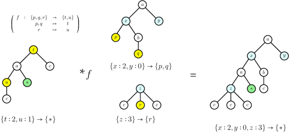
Figure 13. Composition of some multimorphisms of $\mathcal{TR}^{\mathrm{m}}$.

We now set $\mathcal{TR}=(\mathcal{TR}^{\mathrm{m}})_{\mathrm{aff}}$; while objects of $(\mathcal{TR}^{\mathrm{m}})_{\mathrm{aff}}$ are supposed to be families of finite sets $(A_{i})_{i\in I}$, in the sequel, we sometimes identify them with the ranked alphabets $(I,A)$ in $\mathcal{TR}$ for notational convenience. As such, the notation ${\bf R}\otimes{\bf S}$ corresponds to the expected tensorial product in $\mathcal{TR}$.

We are now ready to define our first tree streaming setting.

$\mathfrak{TR}$ is the tree streaming setting $(\mathcal{TR},\otimes,\top,\mathcal{I}(\varnothing),{\llparenthesis-\rrparenthesis})$, where ${\llparenthesis-\rrparenthesis}$ is the canonical isomorphism $\mathsf{Hom}_{\mathcal{TR}}\left(\top,\mathcal{I}(\varnothing)\right)\cong\mathsf{Hom}_{\mathcal{TR}^{\mathrm{m}}}\left(()_{\varnothing},\varnothing\right)\cong\mathbf{LTree}_{\bf\Gamma}(\varnothing)\cong\mathbf{Tree}({\bf\Gamma})$ (where $()_{\varnothing}$ is the empty family).

Call $\mathcal{TR}^{\mathrm{m},\leq 1}$ the full submulticategory of $\mathcal{TR}^{\mathrm{m}}$ whose objects are empty or singleton sets, and $\mathcal{TR}^{\leq 1}\cong\mathcal{TR}^{\mathrm{m},\leq 1}_{\mathrm{aff}}$ to be the corresponding full subcategory of $\mathcal{TR}$. The monoidal structure of $\mathcal{TR}$ restricts to $\mathcal{TR}^{\leq 1}$ without any difficulty, and that $\mathcal{I}(\varnothing)$ is an object of $\mathcal{TR}^{\leq 1}$. This means that $\mathfrak{TR}$ has a restriction to a streaming setting $\mathfrak{TR}^{\leq 1}$.

While $\mathfrak{TR}^{\leq 1}$ turns out to be more elementary and a good building block toward the definition of usual BRTTs, it is easier to show the monoidal closure of $\mathfrak{TR}_{\oplus\with}$ than $\mathfrak{TR}^{\leq 1}$. Thankfully, it turns out that the expressiveness of BRTTs over $\mathfrak{TR}$ and $\mathfrak{TR}^{\leq 1}$ is the same.

For one direction, there is a morphism $\mathfrak{TR}^{\leq 1}\to\mathfrak{TR}$ corresponding to the embedding $\mathcal{TR}^{\leq 1}\to\mathcal{TR}$. For the other direction, we exploit Theorem 55. The proof involves some combinatorics, but nothing surprising as it amounts to the classical decomposition of multi-hole trees into families of single-hole trees as found in e.g. [AD17, §3.5].

Lemma 57.

There is a morphism of streaming settings $\mathfrak{TR}\to\mathfrak{TR}^{\leq 1}_{\oplus}$.

Proof 5.2 (Proof sketch).

We focus on giving enough ingredients to define the underlying (strong) monoidal functor $F:\mathcal{TR}\to\mathcal{TR}^{\leq 1}_{\oplus}$, which is going to preserve $\Bot$ (i.e., we will have $F(\mathcal{I}(\varnothing))\cong\iota_{\oplus}(\mathcal{I}(\varnothing))$).

Rather than giving a direct explicit construction of $F$ (which is rather tedious over morphisms), we obtain it as a composition of two strong monoidal functors: the strong monoidal embedding $\iota_{\oplus}:\mathcal{TR}\to\mathcal{TR}_{\oplus}$ and a functor $R:\mathcal{TR}_{\oplus}\to\mathcal{TR}^{\leq 1}_{\oplus}$ right adjoint to the inclusion $I:\mathcal{TR}^{\leq 1}_{\oplus}\to\mathcal{TR}_{\oplus}$.

$I$ is strong symmetric monoidal. Therefore, by [Mel09, Proposition 14, Section 5.17], once we construct $R$ right adjoint to $I$, it comes equipped with a canonical lax monoidal structure. Furthermore, since we want $I\dashv R$, we can use the implicit characterization of adjoints given in [ML98, item (iv), Theorem 2, Section IV.1]: to define $R$, it suffices to give the value of $R\left(A\right)$ for every object $A\in\mathsf{Obj}(\mathcal{TR}_{\oplus})$ and counit maps $\epsilon_{A}:I(R(A))\to A$ such that, for every object $B\in\mathsf{Obj}(\mathcal{TR}^{\leq 1}_{\oplus})$ and map $h\in\mathsf{Hom}_{\mathcal{TR}_{\oplus}}\left(I(B),A\right)$, there is a unique $\widetilde{h}\in\mathsf{Hom}_{\mathcal{TR}^{\leq 1}_{\oplus}}\left(R(A),B\right)$ such that the following diagram commutes

So we only need to define $R(A)$ and $\epsilon_{A}$ to obtain our functor $R$; once those are defined, we leave checking that the universal property holds to the reader. We first focus on the case where $A=\iota_{\oplus}(\mathcal{I}(U))$ for some finite set $U$. Recall that a single-letter alphabet $\mathcal{I}(U)$, when seen as an object of $\mathcal{TR}$, should be should be intuitively regarded as a register containing a tree with $U$-many holes. If ${|U|}\leq 1$, we may simply take $R(\iota_{\oplus}(\mathcal{I}(U)))=\iota_{\oplus}(\mathcal{I}(U))$. Otherwise, ${|U|}\geq 2$ and $\mathcal{I}(U)$ is not an object $\mathcal{TR}^{\leq 1}$; in that case, we use the following recursive definition

$$R(\iota_{\oplus}(\mathcal{I}(U)))\leavevmode\nobreak\ \leavevmode\nobreak\ \leavevmode\nobreak\ =\leavevmode\nobreak\ \leavevmode\nobreak\ \leavevmode\nobreak\ \mathcal{I}(1)\leavevmode\nobreak\ \leavevmode\nobreak\ \otimes\leavevmode\nobreak\ \leavevmode\nobreak\ \bigoplus\limits_{b\in\Gamma}\bigoplus\limits_{\begin{subarray}{c}f:U\to\mathrm{ar}(b)\\ \text{nonconstant}\end{subarray}}\bigotimes\limits_{x\in\mathrm{ar}(b)}R(\iota_{\oplus}(\mathcal{I}(f^{-1}(x))))$$

Note that this definition is well-founded because the function $f$ in the second sum is taken to be non constant, so that ${|f^{-1}(x)|}<{|U|}$ for every $x$. While this suffices as a definition of $R(\iota_{\oplus}(\mathcal{I}(U)))$, this might be a bit opaque without having the definition of $\epsilon_{R(\iota_{\oplus}(\mathcal{I}(U)))}$. Before giving that, let us attempt to give an intuitive rationale behind this definition: there is an isomorphism

$$\mathsf{Hom}_{\mathcal{TR}^{\leq 1}_{\oplus}}\left(\top,R(\iota_{\oplus}(\mathcal{I}(U)))\right)\cong\mathbf{LTree}_{\bf\Gamma}(U)$$

which can be nicely pictured, provided we actually compute recursively $R(\iota_{\oplus}(\mathcal{I}(U)))$ and spell out a normal form

$$R(\iota_{\oplus}(\mathcal{I}(U)))\leavevmode\nobreak\ \leavevmode\nobreak\ \leavevmode\nobreak\ \cong\leavevmode\nobreak\ \leavevmode\nobreak\ \leavevmode\nobreak\ \bigoplus_{t\in{\bf PT}(U)}\bigotimes_{n\in N(t)}A_{n}$$

with all $A_{n}=\mathcal{I}(\varnothing)$ or $A_{n}\cong\mathcal{I}(1)$. It is always possible to build a suitable set ${\bf PT}(U)$ simply because all objects of $\mathcal{TR}^{\leq 1}_{\oplus}$ have this shape, but an intuitive definition of what one might call a set of partitioning trees over $U$ is also possible for $\bf PT$, and $N(t)$ would then correspond to the nodes of the trees. We skip defining this notion formally, but note that the announced bijection would then match trees with $U$-many holes with pairs $(t,(u_{i})_{i\in N(t)})$ of a partitioning tree $t$ and a family of trees with at most one-hole $(u_{i})_{i\in N(t)}$. This bijective correspondence is pictured in Figure 14.

 

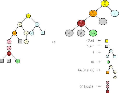
Figure 14. Decomposition of a multi-hole tree $\mathbf{LTree}_{\{a:2,b:1,c:0,d:3\}}(\{x,y,z,t\})$ as a tuple consisting of a partitioning tree and trees with at most one hole.

Now, we define $\epsilon_{R(\iota_{\oplus}(\mathcal{I}(U)))}\in\mathsf{Hom}_{\mathcal{TR}^{\leq 1}_{\oplus}}\left(I(R(\iota_{\oplus}(\mathcal{I}(U)))),\iota_{\oplus}(\mathcal{I}(U))\right)$, by induction over the size of $U$. If ${|U|}\leq 1$, we take $\epsilon_{R(\iota_{\oplus}(\mathcal{I}(U)))}:\iota_{\oplus}(\mathcal{I}(U))\to\iota_{\oplus}(\mathcal{I}(U))$ to be the identity. Otherwise, we need to define a map

$$g_{U}\leavevmode\nobreak\ \leavevmode\nobreak\ :\leavevmode\nobreak\ \leavevmode\nobreak\ I\left(\bigoplus_{b\in\Gamma}\bigoplus_{\begin{subarray}{c}f:U\to\mathrm{ar}(b)\\ \text{nonconstant}\end{subarray}}\bigotimes_{x\in\mathrm{ar}(b)}R(\iota_{\oplus}(\mathcal{I}(f^{-1}(x))))\right)\leavevmode\nobreak\ \leavevmode\nobreak\ \longrightarrow\leavevmode\nobreak\ \leavevmode\nobreak\ \iota_{\oplus}(\mathcal{I}(U))$$

or, equivalently, a family of $\mathcal{TR}_{\oplus}$-maps indexed by $b\in\Gamma$ and $f:U\to\mathrm{ar}(b)$ non-constant

$$g_{b,f}\leavevmode\nobreak\ \leavevmode\nobreak\ :\leavevmode\nobreak\ \leavevmode\nobreak\ \bigotimes_{x\in\mathrm{ar}(b)}I(R(\iota_{\oplus}(\mathcal{I}(f^{-1}(x)))))\leavevmode\nobreak\ \leavevmode\nobreak\ \longrightarrow\leavevmode\nobreak\ \leavevmode\nobreak\ \iota_{\oplus}(\mathcal{I}(U))$$

By the induction hypothesis, we have a family of $\mathcal{TR}_{\oplus}$-maps $(g_{x})_{x\in\mathrm{ar}(b)}$

$$g_{x}\leavevmode\nobreak\ \leavevmode\nobreak\ :\leavevmode\nobreak\ \leavevmode\nobreak\ I(R(\iota_{\oplus}(\mathcal{I}(f^{-1}(x)))))\leavevmode\nobreak\ \leavevmode\nobreak\ \longrightarrow\leavevmode\nobreak\ \leavevmode\nobreak\ \iota_{\oplus}(\mathcal{I}(f^{-1}(x)))$$

We define $g_{b,f}$ as the composite

$$\bigotimes_{x\in\mathrm{ar}(b)}I(R(\iota_{\oplus}(\mathcal{I}(f^{-1}(x)))))\leavevmode\nobreak\ \xrightarrow{\leavevmode\nobreak\ \leavevmode\nobreak\ \bigotimes_{x}g_{x}\leavevmode\nobreak\ \leavevmode\nobreak\ }\leavevmode\nobreak\ \displaystyle\bigotimes_{x\in\mathrm{ar}(b)}\iota_{\oplus}(\mathcal{I}(f^{-1}(x)))\leavevmode\nobreak\ \xrightarrow{\leavevmode\nobreak\ \leavevmode\nobreak\ \overline{b}\leavevmode\nobreak\ \leavevmode\nobreak\ }\leavevmode\nobreak\ \iota_{\oplus}(\mathcal{I}(U))$$

where $\overline{b}$ is obtained from the map of $\mathcal{TR}^{\mathrm{m}}$ which intuitively takes a family $(t_{x})_{x\in\mathrm{ar}(b)}$ of trees into a single tree $b((t_{x})_{x\in\mathrm{ar}(b)})$ (officially, the tree $b((*)_{x\in\mathrm{ar}(b)})\in\mathbf{LTree}_{\bf\Gamma}(\mathcal{O}(U))$.

Now, $R$ is defined on objects of the shape $\iota_{\oplus}(\mathcal{I}(U))$, as well as $\epsilon$, so we need to extend this to the whole category $\mathcal{TR}_{\oplus}$. Recall that every object $A$ of $\mathcal{TR}_{\oplus}$ can be written as $A=\bigoplus_{v\in V}\bigotimes_{j\in J_{u}}\iota_{\oplus}(\mathcal{I}(U_{j}))$. In the end, the functor $R$ is expected to be strong monoidal, and we may force it to preserve coproducts, so we set

$$R(A)\leavevmode\nobreak\ \leavevmode\nobreak\ =\leavevmode\nobreak\ \leavevmode\nobreak\ \bigoplus_{v\in V}\bigotimes_{j\in J_{u}}R(\iota_{\oplus}(\mathcal{I}(U_{j})))\qquad\qquad\qquad\epsilon_{A}\leavevmode\nobreak\ \leavevmode\nobreak\ =\leavevmode\nobreak\ \leavevmode\nobreak\ \bigoplus_{v\in V}\bigotimes_{j\in J_{u}}\epsilon_{\iota_{\oplus}(\mathcal{I}(U_{j}))}$$

5.3.2. Relationship to $\lambda\ell^{\oplus\with}$

Recall that if ${\bf\Gamma}=\{a_{1}:A_{1},\ldots,a_{k}:A_{k}\}$ is an output alphabet, we call $\widetilde{\bf\Gamma}$ the context $a_{1}:\mathbbl{o}\multimap\ldots\multimap\mathbbl{o},\ldots,a_{k}:\mathbbl{o}\multimap\ldots\multimap\mathbbl{o}$ where the type of $a_{i}$ has ${|A_{i}|}$ arguments. Definition 3.3 provides us with a suitable affine monoidal closed category $\mathcal{L}(\widetilde{\bf\Gamma})$, which we still call $\mathcal{L}$ when $\widetilde{\bf\Gamma}$ is clear from context. Since we have a monoidal product, we may easily adapt Definition 3.3 to get a tree streaming setting $\mathfrak{L}$. Then we may relate $\lambda\ell^{\oplus\with}$-definability to (single-state) $\mathfrak{L}$-BRTT.

Lemma 58.

Computability by single-state $\mathfrak{L}$-BRTTs and $\lambda\ell^{\oplus\with}$-definability are equivalent for functions $\mathbf{Tree}({\bf\Sigma})\to\mathbf{Tree}({\bf\Gamma})$.

Proof 5.3 (Proof idea).

This is proven in a similar way as Lemma 24, based on the syntactic Lemma 25. The proof is even more straightforward as there is no mismatch between the processing of trees by BRTTs and $\lambda\ell^{\oplus\with}$-terms working with Church encodings, contrary to SSTs for strings (which operate top-down rather than bottom-up when regarding strings as trees).

We can now notice that $\mathfrak{L}$-BRTTs are more expressive than $\mathcal{TR}^{\leq 1}$-BRTTs thanks to the notion of streaming setting morphisms, much like with strings (this generalizes Lemma 26).

Lemma 59.

There is a morphism of streaming settings $\mathfrak{TR}\to\mathfrak{L}$.

Proof 5.4 (Proof sketch).

Let us focus on the underlying functor $F:\mathcal{TR}\to\mathcal{L}$. For objects (which are finite sets), we put

$$F\left(\bigotimes_{i\in I}U_{i}\right)=\bigotimes_{i\in I}\left(\left(\mathbbl{o}^{\otimes U_{i}}\multimap\mathbbl{o}\right)\with\mathbf{I}\right)$$

A multimorphism $f\in\mathsf{Hom}_{\mathcal{TR}^{\mathrm{m}}}\left((U_{i})_{i\in I},V\right)$ is an element of $\mathbf{LTree}_{\bf\Gamma}\left(\left(\bigotimes_{i\in I}\mathcal{I}(U_{i})\right)\otimes\mathcal{O}(V)\right)$ which has a Church encoding $\underline{f}$ which has a type isomorphic to $\bigotimes_{i\in I}\left(\mathbbl{o}^{\otimes{U_{i}}}\multimap\mathbbl{o}\right)\multimap\mathbbl{o}$, and thus embeds into $F\left(\bigotimes_{i\in I}U_{i}\right)$ through well-typed term $\iota$. We take $F(f_{\mathrm{aff}})=\lambda x.\iota\;\underline{f}$, and extend this definition to arbitrary morphisms $(f,(\alpha_{j})_{j}):\bigotimes_{i\in I}U_{i}\to\bigotimes_{j\in J}V_{j}$ in $\mathcal{TR}$ by first using the second projection $\pi_{2}$ to restrict to the case where ${\sf{dom}}(f)=I$, and then by piecing together the $F((\alpha_{j})_{\mathrm{aff}})$.

Corollary 60.

There is a morphism of streaming settings $\mathfrak{TR}_{\oplus\with}\to\mathfrak{L}$.

Proof 5.5 (Proof idea).

Starting from Lemma 59, we have a functor $\mathcal{TR}\to\mathcal{L}$. Since $\mathcal{L}$ has all products and coproducts, the universal properties of the $(-)_{\with}$ and $(-)_{\oplus}$ completion yield a functor $F:\mathcal{TR}_{\oplus\with}\to\mathcal{L}$. The monoidal structure of the initial functor $\mathcal{TR}\to\mathcal{L}$ can be lifted accordingly. For any finite family of objects $(((A_{k})_{k\in K_{j}})_{j\in J_{i}})_{i\in I}$ sitting in a symmetric monoidal closed category with products and coproducts, there are canonical morphisms

$$\left(\bigoplus_{u\in U}\bigwith_{x\in X_{u}}A_{x}\right)\otimes\left(\bigoplus_{v\in V}\bigwith_{v\in Y_{v}}B_{y}\right)\leavevmode\nobreak\ \leavevmode\nobreak\ \longrightarrow\leavevmode\nobreak\ \leavevmode\nobreak\ \bigoplus_{(u,v)\in U\times V}\bigwith_{(x,y)\in X_{u}\times Y_{v}}A_{x}\otimes B_{y}$$

which are not isomorphisms in general, but constitute the non-trivial part of the lax monoidal structure of $F$; $m^{0}:\mathbf{I}\to F(\mathbf{I})$ is actually the identity.

5.4. $\mathfrak{TR}_{\with}$-BRTTs coincide with regular functions, via coherence spaces

We define a streaming setting $\mathfrak{TR}^{\incoh}$ and its restriction $\mathfrak{TR}^{\incoh,\leq 1}$ (with respective underlying categories $\mathcal{TR}^{\incoh}$, $\mathcal{TR}^{\incoh,\leq 1}$) so that $\mathfrak{TR}^{\incoh,\leq 1}$-BRTTs coincide with Alur and D’Antoni’s notion of single-use-restricted BRTT [AD17], which they showed to characterize regular tree functions. We then show that there are morphisms of streaming settings $\mathfrak{TR}_{\with}\to\mathfrak{TR}^{\incoh}\to\mathfrak{TR}_{\with}$ and thus establish that $\mathfrak{TR}_{\with}$-BRTTs capture exactly regular tree functions.

Much like $\mathcal{TR}$, the category $\mathcal{TR}^{\incoh}$ is obtained by applying a generic construction to $\mathcal{TR}^{\mathrm{m}}$, taking weak symmetric multicategories to symmetric affine monoidal categories. In particular, objects of $\mathcal{TR}^{\incoh}$ will consist of formal tensor products of objects of $\mathcal{TR}^{\mathrm{m}}$. The main difference is that morphisms of $\mathcal{TR}^{\incoh}$ will induce a dependency relation $D\subseteq I\times J$ over indexing sets, rather than a partial function $J\rightharpoonup I$. This corresponds to a relaxation of the copylessness condition. However, objects of $\mathcal{TR}^{\incoh}$ will also be equipped with a conflict relation $\incoh$ over their indexed sets, and $D$ will be required to satisfy a linearity constraint. Calling $\coh$ the dual coherence relation such that $x\coh y$ is equivalent to $x=y\vee\neg(x\incoh y)$, if we have $(i,j)\in D$ and $(i^{\prime},j^{\prime})\in D$, the linearity constraint enforces

$$j\coh_{J}j^{\prime}\leavevmode\nobreak\ \leavevmode\nobreak\ \Rightarrow\leavevmode\nobreak\ \leavevmode\nobreak\ i\coh_{I}i^{\prime}\qquad\text{and}\qquad i\incoh_{I}i^{\prime}\leavevmode\nobreak\ \leavevmode\nobreak\ \Rightarrow\leavevmode\nobreak\ \leavevmode\nobreak\ j\incoh_{J}j^{\prime}$$

This corresponds to the single use restriction imposed on BRTTs [AD17, §2.1], whose introduction was motivated in Section 2.2.3. The BRTT that we gave for the “conditional swap” function in Example 5 is single-use-restricted according to the above by taking its two registers (i.e. objects of $\mathcal{TR}^{\mathrm{m}}$) to be in conflict. But as our choice of notation and vocabulary suggests, this is also related to the category of (finite) coherence spaces, the first denotational model of linear logic [Gir87] (predated by a similar semantics for system F [Gir86]). As far as we know, this observation is new (the conflict relation is denoted by $\mathbf{\eta}$ in [AD17], while $\incoh$ comes from the linear logic literature). The coherence semantics of the linear $\lambda$-calculus has been used in particular by Gallot, Lemay and Salvati [GLS20] to analyze a top-down tree transducer model containing linear $\lambda$-terms. Unlike them, we do not use coherence spaces as a semantics here; what happens here is much closer the use of a coherence/conflict relation to handle additive connectives – we will indeed show a connection with the $\with$-completion – in proof nets, see [Gir96, Appendix A.1] and [HH16].

[see e.g. [Gir95, §2.2.3]] A coherence space $I$ is a pair $(\|I\|,\coh_{I})$ of a set $\|I\|$, called the web, and a binary reflexive symmetric relation $\coh_{I}$ over $\|I\|$ called the coherence relation. As usual, given a coherence relation $\coh$, we write $\incoh$ for the dual defined by $i\incoh i^{\prime}\Leftrightarrow(i=i^{\prime}\vee\neg(i\coh i^{\prime}))$. Finite coherence spaces are those coherence spaces whose webs are finite. A linear map of coherence spaces $f:I\to J$ is a relation $f\subseteq\|I\|\times\|J\|$ such that, whenever $(i,j)\in f$ and $(i^{\prime},j^{\prime})\in f$, we have

$$i\coh_{I}i^{\prime}\leavevmode\nobreak\ \leavevmode\nobreak\ \Rightarrow\leavevmode\nobreak\ \leavevmode\nobreak\ j\coh_{J}j^{\prime}\qquad\text{and}\qquad j\incoh_{J}j^{\prime}\leavevmode\nobreak\ \leavevmode\nobreak\ \Rightarrow\leavevmode\nobreak\ \leavevmode\nobreak\ i\incoh_{I}i^{\prime}$$

Note that these are the converse implications of those stated above for BRTTs.

The diagonal $\{(i,i)\mid i\in\|I\|\}$ is a linear map $I\to I$ and the relational composition of two linear maps $I\to J\to K$ is again a linear map, so that we have a category ${\sf FinCoh}$ whose objects are coherence spaces and morphisms are linear maps.

${\sf FinCoh}$, equipped with the tensorial product

$$(\|I\|,\coh_{I})\otimes(\|J\|,\coh_{J})=(\|I\|\times\|J\|,\coh_{I}\times\coh_{J})$$

and dualizing object $(1,1\times 1)$, is a well-studied $*$-autonomous category with cartesian products and coproducts. The latter may be defined pointwise as

$$(\|I\|,\coh_{I})\oplus(\|J\|,\coh_{J})=(\|I\|+\|J\|,\;\coh_{I\oplus J})$$

where $\coh_{I\oplus J}$ is the smallest relation such that

$$\mathsf{in}_{1}(i)\coh_{I\oplus J}\mathsf{in}_{1}(i^{\prime})\ \;\text{when}\ \;i\coh_{I}i^{\prime}\qquad\text{and}\qquad\mathsf{in}_{2}(j)\coh_{I\oplus J}\mathsf{in}_{2}(j^{\prime})\ \;\text{when}\ \;j\coh_{J}j^{\prime}$$

Dualizing an object corresponds to moving from $\coh$ to $\incoh$, i.e. $(\|I\|,\coh_{I})^{\bot}=(\|I\|,\incoh_{I})$, and the product is $I\with J=(I^{\bot}\oplus J^{\bot})^{\bot}$.

With this in mind, we can describe how to turn a multicategory into an affine monoidal category where monoidal products may be indexed by coherence spaces. The construction has a vague family resemblance with the coherence completion of categories introduced by Hu and Joyal [HJ99], but appears to have quite different properties.

Let $\mathcal{M}$ be a weak symmetric multicategory. We define $\mathcal{M}_{\mathrm{coh}}$ to be the category

• whose objects are pairs $(X,(R_{x})_{x\in\|X\|})$ where $X$ is a finite coherence space and $(R_{x})_{x\in\|X\|}$ a family of objects of $\mathcal{M}$. We suggestively write them $\bigodot_{x\in X}R_{x}$.

• whose morphisms

  $$(f,(\alpha_{y})_{y\in\|Y\|})\in\mathsf{Hom}_{\mathcal{M}_{\mathrm{coh}}}\left(\bigodot_{x\in X}R_{x},\bigodot_{y\in Y}S_{y}\right)$$

  are pairs consisting of a linear map $f\in\mathsf{Hom}_{{\sf FinCoh}}\left(Y,X\right)$ and a family of multimorphisms $\alpha_{y}\in\mathsf{Hom}_{\mathcal{M}}\left((R_{x})_{x\in f(y)},S_{y}\right)$.

• whose identities are pairs $(\mathrm{id}_{X},(\mathrm{id}_{R_{x}})_{x\in\|X\|})$.

• where the composition of

  $$(f,(\alpha_{y})_{y\in\|Y\|})\in\mathsf{Hom}\left(\bigodot_{x\in X}R_{x},\bigodot_{y\in Y}S_{y}\right)\leavevmode\nobreak\ \leavevmode\nobreak\ \text{and}\leavevmode\nobreak\ \leavevmode\nobreak\ (g,(\beta_{z})_{z\in\|Z\|})\in\mathsf{Hom}\left(\bigodot_{y\in Y}S_{y},\bigodot_{z\in Z}T_{z}\right)$$

  is $(f\circ g,(\beta_{z}*(\alpha_{y})_{y\in g(z)})_{z\in Z})$.

We set $\mathcal{TR}^{\incoh}=(\mathcal{TR}^{\mathrm{m}})_{\mathrm{coh}}$ and $\mathcal{TR}^{\incoh,\leq 1}$ to be its full subcategory consisting of objects $\bigodot_{x\in X}A_{x}$ where each $A_{x}$ is either empty or a singleton (so that $\mathcal{TR}^{\incoh,\leq 1}$ is isomorphic to $(\mathcal{TR}^{\mathrm{m},\leq 1})_{\mathrm{coh}}$).

Proposition 61.

BRTTs over the restricted tree streaming setting $\mathfrak{TR}^{\incoh,\leq 1}$ compute exactly the regular tree functions.

Proof 5.6.

By virtue of being equivalent to Alur and D’Antoni’s notion of single-use-restricted BRTT [AD17]. We point the reader to Appendix A for a self-contained definition of those not involving categories, and leave it as an exercise to formally match those two descriptions. Although [AD17] and our Appendix A only consider BRTTs over binary trees, the proof of equivalence between the latter and regular tree functions goes through macro tree transducers (with regular look-ahead and single use restriction) which are known to compute regular functions for trees over arbitrary ranked alphabets [EM99], so everything can be made to work out with arbitrary arities in the end.

This being done, the remainder of this section does not depend on $\mathcal{TR}^{\mathrm{m}}$; the arguments apply to any weak symmetric multicategory $\mathcal{M}$ and designated object $\Bot\in\mathsf{Obj}(\mathcal{M})$.

Accordingly, fix such an $\mathcal{M}$ and a $\Bot$ for the remainder of this section. Fix also a set $O$ and a map ${\llparenthesis-\rrparenthesis}:\mathsf{Hom}_{\mathcal{M}}\left((\cdot)_{\varnothing},\Bot\right)\to O$.

Proposition 62.

$\mathcal{M}_{\mathrm{coh}}$ has a terminal object, given by the unique family over the empty coherence space, and can be equipped with a symmetric monoidal affine structure $(\otimes,\top)$ where

$$\left(\bigodot_{i\in I}A_{i}\right)\otimes\left(\bigodot_{j\in J}B_{j}\right)\leavevmode\nobreak\ \leavevmode\nobreak\ =\leavevmode\nobreak\ \leavevmode\nobreak\ \bigodot_{x\in I\with J}\left\{\begin{array}[]{ll}A_{i}&\text{if $x=\mathsf{in}_{1}(i)$}\\ B_{j}&\text{if $x=\mathsf{in}_{2}(j)$}\\ \end{array}\right.$$

and $I\with J$ designates the cartesian product in ${\sf FinCoh}$.

Proof 5.7.

Left to the reader. Strictly speaking, later developments will depend on the precise structure itself and not merely on its existence, but there is a single sensible choice of bifunctorial action and structural morphisms making the above a monoidal product.

Remark 63.

To start making sense of the use of the cartesian product of ${\sf FinCoh}$, there is a useful analogy with $\mathcal{M}_{\mathrm{aff}}$ here. There is a projection functor $\mathcal{M}_{\mathrm{aff}}\to{\sf PartFinSet}$ where ${\sf PartFinSet}$ is the category of finite sets and partial functions. The tensorial product of $\mathcal{M}_{\mathrm{aff}}$ required a coproduct at the level of indices. Here, we have a projection functor $\mathcal{M}_{\mathrm{coh}}\to{\sf FinCoh}^{\mathrm{op}}$, and we again use a coproduct at the level of indices (which becomes a product due to the contravariance).

We call $\mathfrak{M}_{\mathrm{aff}}$ the tree streaming setting based on $\mathcal{M}_{\mathrm{aff}}$, $\Bot$ and ${\llparenthesis-\rrparenthesis})$, and $\mathfrak{M}_{\mathrm{coh}}$ the corresponding tree streaming setting based on $\mathcal{M}_{\mathrm{coh}}$.

Proposition 64.

There is a full and faithful strong monoidal functor $\mathcal{M}_{\mathrm{aff}}\to\mathcal{M}_{\mathrm{coh}}$ extending to a morphism of streaming setting $\mathfrak{M}_{\mathrm{aff}}\to\mathfrak{M}_{\mathrm{coh}}$.

Proof 5.8.

Call $F$ this functor, and, for any set $I$, write $\Delta$ for the functor ${\sf PartFinSet}\to{\sf FinCoh}$ taking a set $I$ to the discrete coherence space $\Delta(I)=(I,\{(i,i)\mid i\in I\})$. Note that we have $\Delta(I)^{\bot}=(I,I\times I)$, which may be regarded as the codiscrete coherence space generated by $I$. On objects of $\mathcal{M}_{\mathrm{aff}}$, we define $F$ as

$$F\left(\bigotimes_{i\in I}A_{i}\right)=\bigodot_{i\in\Delta(I)^{\bot}}A_{i}$$

For morphisms $(f,(\alpha_{j})_{j\in J})\in\mathsf{Hom}_{\mathcal{M}_{\mathrm{aff}}}\left(\bigotimes_{i\in I}A_{i},\bigotimes_{j\in J}B_{j}\right)$, we set

$$F(f,(\alpha_{j})_{j\in J})=(\{(j,i)\mid j=f(i)\},(\alpha_{j})_{j\in J})$$

It is rather straightforward to check that $F$ is indeed full, faithful and strong monoidal, and the extension to a morphism $\mathfrak{M}_{\mathrm{aff}}\to\mathfrak{M}_{\mathrm{coh}}$ is immediate.

Proposition 65.

$\mathcal{M}_{\mathrm{coh}}$ also has cartesian products, which may be defined as

$$\left(\bigodot_{i\in I}A_{i}\right)\with\left(\bigodot_{j\in J}B_{j}\right)\leavevmode\nobreak\ \leavevmode\nobreak\ =\leavevmode\nobreak\ \leavevmode\nobreak\ \bigodot_{x\in I\oplus J}\left\{\begin{array}[]{ll}A_{i}&\text{if $x=\mathsf{in}_{1}(i)$}\\ B_{j}&\text{if $x=\mathsf{in}_{2}(j)$}\\ \end{array}\right.$$

(The proof is left to the reader.) Therefore, we can extend Proposition 64:

Corollary 66.

There is a functor $E:(\mathcal{M}_{\mathrm{aff}})_{\with}\to\mathcal{M}_{\mathrm{coh}}$ that is full, faithful and lax (but not strong) monoidal, extending to a morphism of streaming settings $(\mathfrak{M}_{\mathrm{aff}})_{\with}\to\mathfrak{M}_{\mathrm{coh}}$.

In the following proof and the rest of this section, we write explicitly $\mathbf{I}_{\mathrm{coh}}$ for the monoidal unit of $\otimes$ in $\mathcal{M}_{\mathrm{coh}}$ and ${\mathbf{I}_{\mathrm{aff}}}_{\with}$ for the unit in $(\mathcal{M}_{\mathrm{aff}})_{\with}$.

Proof 5.9 (Proof idea).

The universal property of the free product completion defines $E$ as the unique product-preserving functor extending the functor of Proposition 64. It remains to equip it with a lax monoidal functor structure. The map $m^{0}:\mathbf{I}_{\mathrm{coh}}\to E({\mathbf{I}_{\mathrm{aff}}}_{\with})$ is an obvious isomorphism, while the natural transformation $m^{2}_{A,B}:E(A)\otimes E(B)\to E(A\otimes B)$ can be obtained via the canonical map

$$\left(\bigwith_{i\in I}A_{i}\right)\otimes\left(\bigwith_{j\in J}B_{j}\right)\to\bigwith_{(i,j)\in I\times J}A_{i}\otimes B_{j}$$

in $\mathcal{M}_{\mathrm{coh}}$ (it exists in all monoidal categories with products).

We can now go the other way around.

Lemma 67.

There is a strong monoidal functor $\mathcal{M}_{\mathrm{coh}}\to(\mathcal{M}_{\mathrm{aff}})_{\with}$, which extends to a morphism of streaming settings $\mathfrak{M}_{\mathrm{coh}}\to(\mathfrak{M}_{\mathrm{aff}})_{\with}$.

Proof 5.10.

For a coherence space $(\|X\|,\coh_{X})$, write $\mathrm{Cl}(X)\subseteq\mathcal{P}(X)$ the set of cliques of $X$

$$\mathrm{Cl}(X)\leavevmode\nobreak\ \leavevmode\nobreak\ =\leavevmode\nobreak\ \leavevmode\nobreak\ \{S\in\mathcal{P}(X)\mid\forall x\;y\in S.\;x\coh_{X}y\}$$

We now define the functor $F:\mathcal{M}_{\mathrm{coh}}\to(\mathcal{M}_{\mathrm{aff}})_{\with}$ on objects as

$$F\left(\bigodot_{x\in X}A_{x}\right)\leavevmode\nobreak\ \leavevmode\nobreak\ =\leavevmode\nobreak\ \leavevmode\nobreak\ \bigwith_{S\in\mathrm{Cl}(X)}\bigotimes_{x\in S}A_{x}$$

As for morphisms, first recall that a morphism $(R,\alpha)\in\mathsf{Hom}_{\mathcal{M}_{\mathrm{coh}}}\left(\bigodot_{x\in X}A_{x},\bigodot_{y\in Y}B_{y}\right)$ consists of a linear map $R\in\mathsf{Hom}_{{\sf FinCoh}}\left(Y,X\right)$ and a family

$$(\alpha_{y})_{y\in\|Y\|}\in\prod_{y\in\|Y\|}\mathsf{Hom}_{\mathcal{M}}\left((A_{x})_{(y,x)\in R},B_{y}\right)$$

We set out to define

$$F(R,\alpha)\in\mathsf{Hom}_{(\mathcal{M}_{\mathrm{aff}})_{\with}}\left(F\left(\bigotimes_{x\in S}A_{x}\right),F\left(\bigotimes_{y\in S^{\prime}}B_{y}\right)\right)$$

recalling that

$$\begin{array}[]{l}\displaystyle\mathsf{Hom}_{(\mathcal{M}_{\mathrm{aff}})_{\with}}\left(F\left(\bigotimes_{x\in S}A_{x}\right),F\left(\bigotimes_{y\in S^{\prime}}B_{y}\right)\right)\\ \\ \hskip 100.00015pt=\leavevmode\nobreak\ \leavevmode\nobreak\ \displaystyle\prod_{S^{\prime}\in\mathrm{Cl}(Y)}\sum_{S\in\mathrm{Cl}(X)}\sum_{f:S\rightharpoonup S^{\prime}}\prod_{y\in S^{\prime}}\mathsf{Hom}_{\mathcal{M}}\left((A_{x})_{x\in f^{-1}(x)},B_{y}\right)\end{array}$$

So fixing $S^{\prime}\in\mathrm{Cl}(Y)$ and recall that $R$ being linear means that we have

$$(y,x)\in R\wedge(y^{\prime},x)\in R\qquad\Rightarrow\qquad\left\{\begin{array}[]{lcll}y\coh_{Y}y^{\prime}&\Rightarrow&x\coh_{X}x^{\prime}&(1)\\ x=x^{\prime}&\Rightarrow&y\incoh_{Y}y^{\prime}&(2)\\ \end{array}\right.$$

In particular, $(1)$ implies that $\{x\in\|X\|\mid(y,x)\in R\}$ is a clique; we take that to be $S$. $(2)$, and the fact that $y\coh_{Y}y^{\prime}\wedge y\incoh_{Y}y^{\prime}\Rightarrow y=y^{\prime}$, imply that $R$ determines a (total) function $S\rightharpoonup S^{\prime}$, which we take to be $f$. Finally, once $y\in S^{\prime}$ is fixed, we pick the component $\alpha_{y}$ to complete the definition, which makes sense as $f^{-1}(y)=\{x\in S\mid(y,x)\in R\}=\{x\in\|X\|\mid(y,x)\in R)\}$. This completes the definition of $F(R,\alpha)$; we leave checking functoriality to the reader.

Now, we turn to defining a morphism of streaming setting $\mathfrak{M}_{\mathrm{coh}}\to(\mathfrak{M}_{\mathrm{aff}})_{\with}$ from $F$. To this end, we must first equip $F$ with a lax monoidal structure, that is to define $(\mathcal{M}_{\mathrm{aff}})_{\with}$-maps

$$m^{0}:{\mathbf{I}_{\mathrm{aff}}}_{\with}\to F(\mathbf{I}_{\mathrm{coh}})\quad\;m^{2}:F\left(\bigodot_{x\in X}A_{x}\right)\otimes F\left(\bigodot_{y\in Y}B_{y}\right)\to F\left(\left[\bigodot_{x\in X}A_{x}\right]\otimes\left[\bigodot_{y\in Y}B_{y}\right]\right)$$

satisfying the relevant coherence diagrams. We do not check them here, but indicate how to build those two maps. $m^{0}$ arises as an obvious isomorphism $F(\mathbf{I}_{\mathrm{coh}})\cong\mathbf{I}_{\mathrm{aff}}$. $m^{2}$ is also an isomorphism, which may be computed as per Figure 15.

$$F\left(\bigodot_{x\in X}A_{x}\right)\otimes F\left(\bigodot_{y\in Y}B_{y}\right)\qquad \cong\qquad\left(\bigwith_{S\in\mathrm{Cl}(X)}\bigotimes_{x\in S}A_{x}\right)\otimes\left(\bigwith_{S^{\prime}\in\mathrm{Cl}(Y)}\bigotimes_{y\in S^{\prime}}B_{y}\right)$$

$$\cong\qquad\bigwith\limits_{\begin{subarray}{c}S\in\mathrm{Cl}(X)\\ S^{\prime}\in\mathrm{Cl}(Y)\end{subarray}}\left(\bigotimes_{x\in X}A_{x}\right)\otimes\left(\bigotimes_{y\in Y}B_{y}\right)$$

$$\cong\qquad\bigwith_{S\in\mathrm{Cl}(X\with Y)}\bigotimes_{z\in S}C_{z}$$

$$\cong\qquad F\left(\bigodot_{z\in X\with Y}C_{z}\right)$$

$$\cong\qquad F\left(\left(\bigodot_{x\in X}A_{x}\right)\otimes\left(\bigodot_{y\in Y}B_{y}\right)\right)$$

Figure 15. The main structural natural isomorphism making the functor $\mathcal{M}_{\mathrm{coh}}\to(\mathcal{M}_{\mathrm{aff}})_{\with}$ strong monoidal, writing $A_{x}$ for $C_{\mathsf{in}_{1}(x)}$ and $B_{y}$ for $C_{\mathsf{in}_{2}(y)}$.

Finally, there is a canonical isomorphism $F(\Bot)\cong\Bot$ which allows to complete the definition of the morphism $\mathfrak{M}_{\mathrm{coh}}\to(\mathfrak{M}_{\mathrm{aff}})_{\with}$.

We thus conclude this section by first specializing the above to the case $\mathcal{M}=\mathcal{TR}^{\leq 1}$, and then making a final tangential observation.

Lemma 68.

There are morphisms of streaming settings $\mathfrak{TR}^{\leq 1}_{\with}\to\mathfrak{TR}^{\incoh,\leq 1}\to\mathfrak{TR}^{\leq 1}_{\with}$. In particular, $\mathfrak{TR}^{\leq 1}_{\with}$-BRTTs compute exactly the regular functions.

Remark 69.

One idea that one could take from Hu and Joyal’s coherence completion [HJ99] – but that we do not explore further here – is to look at objects whose indexing coherence spaces are (up to isomorphism) generated from singletons by the $\with/\oplus$ operations of ${\sf FinCoh}$. (Those are called “contractible” in [HJ99, Section 4], and considering coherence spaces as undirected graphs, this corresponds to the classical notion of cograph in combinatorics.)

In the case of the coherence completion of some category $\mathcal{C}$, the full subcategory spanned by such objects turns out to be the free completion of $\mathcal{C}$ under finite products and coproducts (which differs from our $(-)_{\oplus\with}$ in not making ‘$\with$’ distribute over ‘$\oplus$’); this is formalized as a universal property in [HJ99, Theorem 4.3]. In the same vein, we conjecture that the full subcategory of $\mathcal{M}_{\mathrm{coh}}$ consisting of cograph-indexed objects – that is, of objects that are generated from those of $\mathcal{M}$ by means of the operations $\otimes/\with$ in $\mathcal{M}_{\mathrm{coh}}$ – is in some way the free affine symmetric monoidal category with products generated by the multicategory $\mathcal{M}$.

5.5. $\mathcal{TR}_{\oplus\with}$ is monoidal closed

Now, we consider the category $\mathcal{TR}_{\oplus\with}$ in the context of trees. Much like with strings, this category is symmetric monoidal monoidal closed with finite products and coproducts, which makes it an ideal target to compile $\lambda\ell^{\oplus\with}$-terms. This structure over $\mathcal{TR}_{\oplus\with}$ is obtained in the same way as for strings: the monoidal product over $\mathcal{TR}$ is defined as distributing over formal sums and products and the usual products and coproducts are created by the $(-)_{\oplus\with}$ completion. Similarly, monoidal closure can be obtained in a generic way once we show that the objects coming from $\mathcal{TR}$ have internal homsets $\mathcal{TR}_{\oplus}$ (echoing Lemma 36). This section is mostly dedicated to proving this fact, whose proof relies on decomposing linear trees in a similar way as in Lemma 57.

Lemma 70.

For any two objects $\bf R$ and $\bf S$ of $\mathcal{TR}$, there is an internal hom $\iota_{\oplus}(\bf R)\multimap\iota_{\oplus}(\bf S)$ in $\mathcal{TR}_{\oplus}$.

Proof 5.11.

First, we treat the special case where ${\bf S}=\mathcal{I}(U)$ for some finite set $U$. To make sense of the definition of $\iota_{\oplus}({\bf R})\multimap\iota_{\oplus}(\mathcal{I}(U))$ it is helpful to notice that it will ultimately induce an isomorphism

$$\mathsf{Hom}_{\mathcal{TR}_{\oplus}}\left(\top,\iota_{\oplus}({\bf R})\multimap\iota_{\oplus}(\mathcal{I}(U))\right)\cong\mathsf{Hom}_{\mathcal{TR}}\left({\bf R},\mathcal{I}(U)\right)\cong\mathbf{LTree}_{\bf\Gamma}({\bf R}\otimes\mathcal{O}(U))$$

so, recalling that objects of $\mathcal{TR}_{\oplus}$ are of the shape $\bigoplus_{i\in I}\bigotimes_{j\in J_{i}}\mathcal{I}(V_{j})$ for $V_{j}$ being finite sets, the operational intuition is that one may code trees with “holes with arity” into some bounded finitary data (which we may informally call a partitioning tree) plus finitely many trees containing holes “without arity”; this bijection is pictured in Figure 16.

 

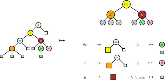
Figure 16. Decomposition of a map of $\mathsf{Hom}_{\mathcal{TR}(\{a:2,b:1,c:0\})}\left(\{x:3,y:3\},\mathcal{I}(7)\right)$ (which is defined as $\mathbf{LTree}_{\{a:2,b:1,c:0\}}(\{x:3,y:3\}\otimes\mathcal{O}(7))$) as a tuple consisting of a partitioning tree and trees without the letters $x$ and $y$.

As with Lemma 57, we will not use this as our official definition for the internal homset, but rather use the following recursive definition:

• If ${\bf R}=\top$, set $\iota_{\oplus}({\bf R})\multimap\iota_{\oplus}(\mathcal{I}(U))\leavevmode\nobreak\ =\leavevmode\nobreak\ \iota_{\oplus}(\mathcal{I}(U))$.

• Otherwise, define $\iota_{\oplus}({\bf R})\multimap\iota_{\oplus}(\mathcal{I}(U))$ as

  $$\bigoplus_{U=V\uplus W}\iota_{\oplus}(\mathcal{I}(V+1))\otimes\left(\bigoplus_{b\in{\bf\Gamma}}\left({\bf R}\multimap_{b}\mathcal{I}(W)\right)\oplus\bigoplus_{r\in R}\left({\bf R}\multimap_{r}\mathcal{I}(W)\right)\right)\\ \\$$

  where ${\bf R}\multimap_{r}\mathcal{I}(W)$ and ${\bf R}\multimap_{b}\mathcal{I}(W)$ are auxiliary definitions which correspond to the following situations (recalling that morphisms can be regarded as trees):

  • $\iota_{\oplus}(\mathcal{I}(V+1))\otimes\left({\bf R}\multimap_{r}\mathcal{I}(W)\right)$ correspond to morphisms such that there is a unique minimal path leading from the root to a node labelled by a letter in $R$, and that letter is $r$. The second component ${\bf R}\multimap_{r}\mathcal{I}(W)$ is meant to include the immediate subtrees of that node while the first $\iota_{\oplus}(\mathcal{I}(V+1))$ contains the tree where a nullary node labeled is inserted instead of that node. The combination of both these data and $r$ allows to recover the original morphism.

  • $\bigoplus_{b\in{\bf\Gamma}}\iota_{\oplus}(\mathcal{I}(V+1))\otimes{\bf R}\multimap_{b}\mathcal{I}(W)$ correspond to all the other morphisms. In such a case there is a topmost node labelled by some letter $b$ of $\bf\Gamma$ with which has at least two distinct immediate subtrees which have at least one node of $R$ each. Similarly to the first subcase, ${\bf R}\multimap_{b}\mathcal{I}(W)$ is intended to include the immediate subtrees of that node labeled by $b$ while $\iota_{\oplus}(\mathcal{I}(V+1))$ contains the tree where a nullary node labeled is inserted instead of that node. The combination of these data and $b$ allows to recover the original morphism.

  Their formal definition is as follows:

  $$\begin{array}[]{*4{>{\displaystyle}l}}&{\bf R}\multimap_{b}\mathcal{I}(W)&=&\bigoplus\limits_{\begin{subarray}{c}f:W\to\mathrm{ar}(b)\\ g:R\to\mathrm{ar}(b)\\ g\text{ nonconstant}\end{subarray}}\bigotimes\limits_{x\in\mathrm{ar}(\Gamma)}\iota_{\oplus}({\bf R}\upharpoonright g^{-1}(x))\multimap\iota_{\oplus}(f^{-1}(x))\\ \\ &{\bf R}\multimap_{r}\mathcal{I}(W)&=&\bigoplus\limits_{\begin{subarray}{c}f:W\to\mathrm{ar}(r)\\ g:R\setminus\{r\}\to\mathrm{ar}(r)\end{subarray}}\bigotimes\limits_{x\in\mathrm{ar}(r)}\iota_{\oplus}({\bf R}\upharpoonright g^{-1}(x))\multimap\iota_{\oplus}(f^{-1}(x))\end{array}$$

  Note that the definitions of $\iota_{\oplus}({\bf R})\multimap\iota_{\oplus}(\mathcal{I}(U))$, ${\bf R}\multimap_{b}\mathcal{I}(W)$ and ${\bf R}\multimap_{r}\mathcal{I}(W)$ mutually depend on one another. Still this is is well-defined as the definitions of ${\bf R}\multimap_{b}\mathcal{I}(W)$ and ${\bf R}\multimap_{r}\mathcal{I}(W)$ only require $\iota_{\oplus}({\bf S})\multimap\iota_{\oplus}(\mathcal{I}(V))$ for ${\bf S}$ strictly smaller than ${\bf R}$.

We now describe the associated evaluation map

$$\mathrm{ev}_{{\bf R},\mathcal{I}(U)}\leavevmode\nobreak\ \leavevmode\nobreak\ :\leavevmode\nobreak\ \leavevmode\nobreak\ (\iota_{\oplus}({\bf R})\multimap\iota_{\oplus}(\mathcal{I}(U)))\otimes{\bf R}\leavevmode\nobreak\ \leavevmode\nobreak\ \longrightarrow\leavevmode\nobreak\ \leavevmode\nobreak\ \mathcal{I}(U)$$

also by recursion over $\bf R$.

• If ${\bf R}=\top$, it is the identity.

• Otherwise, we need to provide maps

  $$\left(\mathcal{I}(V+1)\otimes\left(\bigoplus_{b\in{\bf\Gamma}}\left({\bf R}\multimap_{b}\mathcal{I}(W)\right)\oplus\bigoplus_{r\in R}\left({\bf R}\multimap_{r}\mathcal{I}(W)\right)\right)\right)\otimes{\bf R}\leavevmode\nobreak\ \leavevmode\nobreak\ \longrightarrow\leavevmode\nobreak\ \leavevmode\nobreak\ \mathcal{I}(U)$$

  for every decomposition $U=V\uplus W$, the intuition being that $\mathcal{I}(V+1)$ is a context containing the top of the tree corresponding to the function we want to apply. Therefore, once we provide a map

  $$\left(\bigoplus_{b\in{\bf\Gamma}}\left({\bf R}\multimap_{b}\mathcal{I}(W)\right)\oplus\bigoplus_{r\in R}\left({\bf R}\multimap_{r}\mathcal{I}(W)\right)\right)\otimes{\bf R}\leavevmode\nobreak\ \leavevmode\nobreak\ \longrightarrow\leavevmode\nobreak\ \leavevmode\nobreak\ \mathcal{I}(W)$$

  we may post-compose it with $\mathcal{I}(V+1)\otimes\mathcal{I}(W)\to\mathcal{I}(V+W)\cong\mathcal{I}(V\uplus W)=\mathcal{I}(U)$ to define $\mathrm{ev}_{{\bf R}\multimap\mathcal{I}(U)}$. Recalling that $\otimes$ distributes over $\oplus$, it suffices to provide specialized maps

  $$\mathrm{ev}^{b}_{{\bf R},\mathcal{I}(W)}:{\bf R}\multimap_{b}\mathcal{I}(W)\otimes{\bf R}\to\mathcal{I}(W)\quad\text{and}\quad\mathrm{ev}^{r}_{{\bf R},\mathcal{I}(W)}:{\bf R}\multimap_{r}\mathcal{I}(W)\otimes{\bf R}\to\mathcal{I}(W)$$

  for $b\in\Gamma$ and $r\in R$, which we describe now.

  • For $\mathrm{ev}^{b}_{{\bf R},\mathcal{I}(W)}$, it suffices to define a family of $\mathcal{TR}$-maps indexed by $f:W\to\mathrm{ar}(b)$ and $g:R\to\mathrm{ar}(b)$ with $g$ non-constant

    $$\left(\bigotimes_{x\in\mathrm{ar}(\Gamma)}({\bf R}\upharpoonright g^{-1}(x))\multimap\mathcal{I}(f^{-1}(x))\right)\otimes{\bf R}\leavevmode\nobreak\ \leavevmode\nobreak\ \longrightarrow\leavevmode\nobreak\ \leavevmode\nobreak\ \mathcal{I}(W)$$

    Recall that $b$ can be seen as tree constructor and induces a canonical map

    $$\overline{b}\leavevmode\nobreak\ \leavevmode\nobreak\ :\leavevmode\nobreak\ \leavevmode\nobreak\ \bigotimes_{x\in\mathrm{ar}(b)}\mathcal{I}(f^{-1}(x))\leavevmode\nobreak\ \leavevmode\nobreak\ \longrightarrow\leavevmode\nobreak\ \leavevmode\nobreak\ \mathcal{I}(W)$$

    Using the induction hypothesis, we have evaluation maps

    $$\left(({\bf R}\upharpoonright g^{-1}(x))\multimap\mathcal{I}(f^{-1}(x))\right)\otimes({\bf R}\upharpoonright g^{-1}(x))\leavevmode\nobreak\ \leavevmode\nobreak\ \longrightarrow\leavevmode\nobreak\ \leavevmode\nobreak\ \mathcal{I}(W)$$

    We can then compose $\overline{b}$ with the product of those maps over $x\in\mathrm{ar}(b)$ and then the isomorphism ${\bf R}\cong\bigotimes_{x\in\mathrm{ar}(b)}{\bf R}\upharpoonright f^{-1}(x)$ to conclude the definition of $\mathrm{ev}^{b}_{{\bf R},\mathcal{I}(W)}$.

  • For $\mathrm{ev}^{r}_{{\bf R},\mathcal{I}(W)}$, it suffices to define a family of $\mathcal{TR}$-maps indexed by $f:W\to\mathrm{ar}(r)$ and $g:R\setminus\{r\}\to\mathrm{ar}(r)$

    $$\left(\bigotimes_{x\in\mathrm{ar}(\Gamma)}({\bf R}\upharpoonright g^{-1}(x))\multimap\mathcal{I}(f^{-1}(x))\right)\otimes{\bf R}\leavevmode\nobreak\ \leavevmode\nobreak\ \longrightarrow\leavevmode\nobreak\ \leavevmode\nobreak\ \mathcal{I}(W)$$

    By exploiting the isomorphism ${\bf R}\cong\mathcal{I}(\mathrm{ar}(r))\otimes\bigotimes_{x\in\mathrm{ar}(r)}({\bf R}\upharpoonright g^{-1}(x))$ and using the inductive hypothesis as in the previous case, we obtain a map

    $$\left(\bigotimes_{x\in\mathrm{ar}(\Gamma)}({\bf R}\upharpoonright g^{-1}(x))\multimap\mathcal{I}(f^{-1}(x))\right)\otimes{\bf R}\leavevmode\nobreak\ \leavevmode\nobreak\ \longrightarrow\leavevmode\nobreak\ \leavevmode\nobreak\ \displaystyle\mathcal{I}(\mathrm{ar}(r))\otimes\bigotimes_{x\in\mathrm{ar}(r)}\mathcal{I}(f^{-1}(x))$$

    and we may conclude by post-composing by the map

    $$\mathcal{I}(\mathrm{ar}(r))\otimes\bigotimes_{x\in\mathrm{ar}(r)}\mathcal{I}(f^{-1}(x))\to\mathcal{I}(W)$$

    which is induced by the depth-$2$ tree whose root corresponds to the first component, whose children correspond to the successive elements of $\bigotimes_{x\in\mathrm{ar}(r)}\mathcal{I}(f^{-1}(x))$ and other leaves are in $W$.

While the definition is a bit wordy, there is then little difficulty in checking that this yields the expected universal property.

One needs then to extend the definition for the general case where $\bf S$ is not necessarily $\mathcal{I}(U)$; this is done using a similar approach as for strings, by using a coproduct over partial maps $R\rightharpoonup S$ tracking which letter of the input participates in which letter of the output, and employing the particular case where there is one letter in the output

$$\iota_{\oplus}({\bf R})\multimap\iota_{\oplus}({\bf S})\leavevmode\nobreak\ \leavevmode\nobreak\ =\leavevmode\nobreak\ \leavevmode\nobreak\ \bigoplus_{f:R\rightharpoonup S}\bigotimes_{s\in S}\iota_{\oplus}({\bf R}\upharpoonright f^{-1}(s))\multimap\iota_{\oplus}(\mathcal{I}(\mathrm{ar}(s)))$$

The evaluation function can then be extended and the universal property accordingly lifted to the more general case.

The above lemma tells us that $\mathcal{TR}_{\oplus\with}$ satisfies the premises of Theorem 47, hence:

Theorem 71.

The category $\mathcal{TR}_{\oplus\with}$ has cartesian products, coproducts and a symmetric monoidal closed structure.

Remark 72.

Given the close relationship between the constructions $((-)_{\mathrm{aff}})_{\with}$ and $(-)_{\mathrm{coh}}$, it seems plausible that $(\mathcal{TR}_{\mathrm{coh}})_{\oplus}$ could be monoidal closed (we know that it has products, coproducts and a symmetric monoidal structure). We leave this question to further work.

In other words, $\mathcal{TR}_{\oplus\with}$ provides a categorical semantics for the purely linear fragment of the $\lambda\ell^{\oplus\with}$-calculus. Concretely, by a suitable adaptation of Lemma 27 to tree streaming settings, we finally have:

Corollary 73.

There is a morphism of streaming settings $\mathfrak{L}\to\mathfrak{TR}_{\oplus\with}$.

5.6. Preservation properties of finite completions

We have now proven all of the combinatorial results leading to the main theorem for trees. At this stage, we only need to make explicit a few preservation properties of the completions $(-)_{\oplus}$ and $(-)_{\with}$. We only state the minimal requirements that we need to proceed.

Lemma 74.

Let $\square\in\{\oplus,\with,\oplus\with\}$ and $\mathfrak{C},\mathfrak{D}$ be streaming settings. Then if there is a morphism $\mathfrak{C}\to\mathfrak{D}$, there is also a morphism $\mathfrak{C}_{\square}\to\mathfrak{C}_{\square}$.

Proof 5.12 (Proof idea).

Let us only discuss the case $\square=\oplus$ and assume that we have a streaming setting morphism whose underlying lax monoidal functor is $F:\mathcal{C}\to\mathcal{D}$. Then we consider $F_{\oplus}:\mathcal{C}_{\oplus}\to\mathcal{D}_{\oplus}$ defined using the universal property of $\mathcal{C}_{\oplus}$ from the functor $\iota_{\oplus}\circ F:\mathcal{C}\to\mathcal{D}_{\oplus}$ such that

$$F_{\oplus}\left(\bigoplus_{u\in U}\iota_{\oplus}(C_{u})\right)\leavevmode\nobreak\ \leavevmode\nobreak\ =\leavevmode\nobreak\ \leavevmode\nobreak\ \bigoplus_{u\in U}\iota_{\oplus}(F(C_{u}))$$

so that $F_{\oplus}$ inherits a lax monoidal structure from $F$ by lifting the relevant maps functorially. For instance, we have $\iota_{\oplus}(\mathbf{I})\to\iota_{\oplus}(F(\mathbf{I}))=F_{\oplus}(\mathbf{I})$ for the unit. We leave checking the coherence diagram, the case of the binary tensor to the reader, as well as checking that the rest of the structure of morphisms of streaming settings lift accordingly.

Lemma 75.

Let $\mathfrak{C}$ be a streaming setting. Then there are morphisms of streaming settings $\mathfrak{C}_{\oplus\with}\to(\mathfrak{C}_{\oplus})_{\oplus\with}$ and $(\mathfrak{C}_{\oplus})_{\oplus\with}\to\mathfrak{C}_{\oplus\with}$.

Proof 5.13 (Proof idea).

The first morphism can be obtained using Lemma 74 with the morphism of streaming setting $\mathfrak{C}\to\mathfrak{C}_{\oplus}$ corresponding to $\iota_{\oplus}$. The second morphism can be written as a composite

where $(\mathfrak{Dist}_{\mathfrak{C}})_{\oplus}$ is obtained from a morphism $\mathfrak{Dist}_{\mathfrak{C}}:(\mathfrak{C}_{\oplus})_{\with}\to(\mathfrak{C}_{\with})_{\oplus}$ by Lemma 74. $\mathfrak{Dist}_{\mathfrak{C}}$ itself is built from a functor $D_{\mathcal{C}}:(\mathcal{C}_{\oplus})_{\with}\to(\mathcal{C}_{\with})_{\oplus}$ defined on object following the mantra “products distribute over coproducts”.

$$D_{\mathcal{C}}\left(\bigwith_{x\in X}\iota_{\with}\left(\bigoplus_{u\in U_{x}}\iota_{\oplus}(C_{x,u})\right)\right)\leavevmode\nobreak\ \leavevmode\nobreak\ =\leavevmode\nobreak\ \leavevmode\nobreak\ \bigoplus_{F\in\prod_{x}U_{x}}\iota_{\oplus}\left(\bigwith_{x\in X}\iota_{\with}(C_{x,u})\right)$$

On the other hand, the functor $M:\mathcal{C}$ which is part of $\mathfrak{Mu}_{\mathfrak{C}}$ is obtained by using the universal property of $(-)_{\oplus}$ so that

$$M\left(\bigoplus_{u\in U}\iota_{\oplus}\left(\bigoplus_{v\in V}\iota_{\oplus}(C_{u,v})\right)\right)\leavevmode\nobreak\ \leavevmode\nobreak\ =\leavevmode\nobreak\ \leavevmode\nobreak\ \bigoplus_{(u,v)}\iota_{\oplus}(C_{u,v})$$

5.7. Proof of the main result on trees

We can now give the proof of Theorem 2, which can be summarized as the string of equalities

$$\begin{array}[]{lcl@{\quad}l}\lambda\ell^{\oplus\with}&=&\text{single-state $\mathfrak{L}$-BRTTs}&\text{\small by Lemma\leavevmode\nobreak\ \ref{lem:lamlbrtt}}\\ &=&\text{single-state $\mathfrak{TR}^{\incoh,\leq 1}_{\oplus}$-BRTTs}&(\dagger)\\ &=&\text{$\mathfrak{TR}^{\incoh,\leq 1}$-BRTTs}&\text{\small by Theorem\leavevmode\nobreak\ \ref{thm:oplus-brtt-conservative}}\\ &=&\text{regular tree functions}&\text{\small by Proposition\leavevmode\nobreak\ \ref{prop:brtt-regular}}\end{array}$$

Note that applying Theorem 55 in the last step requires that objects of $\mathcal{TR}^{\incoh,\leq 1}$ have unitary support, which is easily checked for output alphabets ${\bf\Gamma}$ containing at least one letter of arity $\varnothing$. It remains to justify step $(\dagger)$, i.e., that single-state $\mathfrak{L}$-BRTTs and $\mathfrak{TR}^{\incoh,\leq 1}_{\oplus}$-BRTTs are equi-expressive. By Lemma 54, it suffices to have morphisms of streaming settings both ways $\mathfrak{L}\leftrightarrow\mathfrak{TR}^{\incoh,\leq 1}_{\oplus}$ to conclude. They may be obtained as the following composites (where we leave implicit the uses of Lemma 74 and some easily inferrable steps).

6. Conclusion & further work

We have proven that the tree (and string) functions definable at type $\mathrm{Tree}_{\bf\Sigma}[A]\multimap\mathrm{Tree}_{\bf\Gamma}$ in the $\lambda\ell^{\oplus\with}$-calculus correspond exactly to regular functions. To prove the non-trivial left-to-right inclusion, we used a syntactic lemma for $\lambda\ell^{\oplus\with}$-terms allowing to compile those terms into a kind of transducer model using purely linear $\lambda\ell^{\oplus\with}$-terms as its memory ($\mathfrak{L}$-BRTTs). We then showed in a principled way that those transducers are equivalent to the more standard single-use-restricted Bottom-up Ranked Tree Transducers (expressed as $\mathfrak{TR}^{\incoh,\leq 1}$-BRTTs in our framework) which capture regular tree functions. Along the way, we revisited a few results on string transducers under the light of our categorical framework, exhibiting some points of convergence with our semantics for $\lambda\ell^{\oplus\with}$-terms.

There are a number of ways one could plan on expanding this work. We list some of the most relevant problems, regarding the definable functions between strings and trees in various $\lambda$-calculi, that we expect could be tackled using similar methods or minor variations of our setting.

Removing the additive connectives

$\lambda\ell^{\oplus\with}$ features the additive connectives $\oplus$ and $\with$ (as well as the relevant units $0$ and $\top$). A natural question is whether all regular functions are still encodable if we remove access to those connectives and use the $\lambda\kern-0.50003pt\mbox{ \hskip 5.00002pt{1 0 0.4 1} \hbox to0.0pt{\hss\leavevmode\hbox{\set@color\text{a}}} }$-calculus, an affine version of $\lambda\ell^{\oplus\with}$ without those connectives; for strings, this is first half of [NP20, Claim 6.2].

In a sense, we went further than that in showing that $\lambda\ell^{\oplus\with}$-definable functions are regular, since it can be checked that all $\lambda\kern-0.50003pt\mbox{ \hskip 5.00002pt{1 0 0.4 1} \hbox to0.0pt{\hss\leavevmode\hbox{\set@color\text{a}}} }$-definable string-to-string functions are also $\lambda\ell^{\oplus\with}$-definable. However, we did not give evidence for the converse direction, as our encoding of states of BRTTs use the additive connectives. We believe this can be remedied by leveraging our previous work on encoding sequential transducers [NP20, Sections 4-5] (that relies on the highly non-trivial Krohn-Rhodes theorem).

As for functions taking trees as input, we suspect that the $\lambda\kern-0.50003pt\mbox{ \hskip 5.00002pt{1 0 0.4 1} \hbox to0.0pt{\hss\leavevmode\hbox{\set@color\text{a}}} }$-calculus is strictly less expressive than copyless BRTTs ($\mathfrak{TR}$-BRTTs) – in fact, that $\lambda\kern-0.50003pt\mbox{ \hskip 5.00002pt{1 0 0.4 1} \hbox to0.0pt{\hss\leavevmode\hbox{\set@color\text{a}}} }$-terms are even unable to recognize all regular tree languages. We expect that this can be shown by interpreting purely affine $\lambda\kern-0.50003pt\mbox{ \hskip 5.00002pt{1 0 0.4 1} \hbox to0.0pt{\hss\leavevmode\hbox{\set@color\text{a}}} }$-terms into (a variant of) the geometry of interaction semantics mentioned in Example 18. Our intent is to deduce from this that $\lambda\kern-0.50003pt\mbox{ \hskip 5.00002pt{1 0 0.4 1} \hbox to0.0pt{\hss\leavevmode\hbox{\set@color\text{a}}} }$-definable languages can be recognized by tree-walking automata – which are indeed a natural extension to trees of the two-way automata from Example 18 – and some regular tree languages are known to be unrecognizable by such devices [BC08].

Anecdotally, we show in Appendix F that removing the additive disjunction ‘$\oplus$’ from the $\lambda\ell^{\oplus\with}$-calculus while keeping the additive conjunction ‘$\with$’ does not affect the definability of tree functions. While this is a routine application of a continuation-passing-style transformation, the nice thing is that it can be entirely carried out at the level of streaming settings.

Dropping commutativity

The second half of [NP20, Claim 6.2] raised the issue of definable string-to-string transductions in the $\lambda\wp$-calculus, the restriction of the $\lambda\kern-0.50003pt\mbox{ \hskip 5.00002pt{1 0 0.4 1} \hbox to0.0pt{\hss\leavevmode\hbox{\set@color\text{a}}} }$-calculus to a non-commutative multiplicative structure. By analogy with the main result of [NP20], which was that $\lambda\wp$-definable languages are star-free (i.e. first-order definable) while $\lambda\kern-0.50003pt\mbox{ \hskip 5.00002pt{1 0 0.4 1} \hbox to0.0pt{\hss\leavevmode\hbox{\set@color\text{a}}} }$ defines regular languages, the natural guess is that they correspond to first-order regular functions. We expect non-commutative typing to translate into a planarity condition in the above-mentioned category of diagrams (close to a free (non-symmetric) compact-closed category [KL80]).

The situation with trees looks more delicate, although trying to compare the expressiveness of the $\lambda\wp$-calculus with the functional combinators described in [BD20] might be a good starting point.

Duplicating the input

Going to higher complexities, but without escalating to the towers of exponentials definable in the simply-typed $\lambda$-calculus, one natural question is: how expressive are $\lambda\ell^{\oplus\with}$-terms of type $\mathrm{Tree}_{\bf\Sigma}[\kappa]\to\mathrm{Tree}_{\bf\Gamma}$, for purely linear $\kappa$? We expect that this problem could be tackled by reusing our semantic interpretation of purely linear $\lambda\ell^{\oplus\with}$-terms together with a suitable refinement of Lemma 25. Concerning the case of strings, our current conjecture is that the expressible functions have polynomial growth and form a strict subclass of polyregular functions [Boj18, BKL19].

Semantic interpretation of exponentials

One frustrating aspect of our approach is that we need to rely on the normalization of $\lambda\ell^{\oplus\with}$-terms and a special-purpose syntactic lemma to dissect the term under consideration and extract the relevant purely linear subterms before being able to go to semantic interpretations and more high-level arguments. The reason behind this is that our semantics does not interpret the non-linear arrow ‘$\to$’ or, equivalently, a version of the exponential modality ‘$\oc$’ of linear logic. It might be more pleasant to have more general semantic settings with those features that still allow us to show our characterizations. Furthermore, such a setting would be necessary if we hope to tackle the question of the expressiveness of functions $\mathrm{Tree}_{\bf\Sigma}[A]\to\mathrm{Tree}_{\bf\Sigma}$ for general $A$ using semantic tools (this last variant of the problem is equivalent to the setting of the simply-typed $\lambda$-calculus without linearity constraints).

Appendix A Alur and D’Antoni’s Bottom-Up Ranked Tree Transducers

We give here a self-contained definition of the notion of BRTT corresponding to regular tree functions, as they were designed in [AD17]. Since the paper [AD17] is mainly concerned with transducers over unranked trees, the information concerning the definition of BRTTs is spread over its sections 2.1, 3.7 and 3.8. We restrict here to binary trees (as in [AD17, Sections 3.7 and 3.8]) and avoid using multicategories.

[[AD17, p. 31:36]] The set $\mathrm{BinTree}(\Sigma)$ of binary trees over the alphabet $\Sigma$, and the set $\partial\mathrm{BinTree}(\Sigma)$ of one-hole binary trees are generated by the respective grammars

$$T,U::=\lceil\cdot\rceil\mid a\lceil T,U\rceil\quad(a\in\Sigma)\qquad\qquad T^{\prime},U^{\prime}::=\square\mid a\lceil T^{\prime},U\rceil\mid a\lceil T,U^{\prime}\rceil\quad(a\in\Sigma)$$

That is, $\mathrm{BinTree}(\Sigma)$ consists of binary trees whose leaves are all equal to $\langle\rangle$ and whose nodes are labeled with letters in $\Sigma$. As for $\partial\mathrm{BinTree}(\Sigma)$, it contains trees with exactly one leaf labeled $\square$ instead of $\lceil\cdot\rceil$. This “hole” $\square$ is intended to be substituted by a tree: for $T^{\prime}\in\partial\mathrm{BinTree}(\Sigma)$ and $U\in\mathrm{BinTree}(\Sigma)$, $T^{\prime}[U]$ denotes $T^{\prime}$ where $\square$ has been replaced by $U$. [[AD17, p. 31:40]] The binary tree expressions ($E,F$ below, forming the set $\mathrm{ExprBT}(\Sigma,V,V^{\prime})$) and one-hole binary tree expressions ($E^{\prime},F^{\prime}$ below, forming the set $\mathrm{Expr}\partial\mathrm{BT}(\Sigma,V,V^{\prime})$) over the variable sets $V$ and $V^{\prime}$ are generated by the grammar (with $x\in V$, $x^{\prime}\in V^{\prime}$ and $a\in\Sigma$)

$$E,F::=\lceil\cdot\rceil\mid x\mid a\lceil E,F\rceil\mid E^{\prime}[F]\qquad E^{\prime},F^{\prime}:=\square\mid x^{\prime}\mid a\lceil E^{\prime},F\rceil\mid a\lceil E,F^{\prime}\rceil\mid E^{\prime}[F^{\prime}]$$

Given $\rho:V\to\mathrm{BinTree}(\Sigma)$ and $\rho^{\prime}:V^{\prime}\to\partial\mathrm{BinTree}(\Sigma)$, one defines $E(\rho,\rho^{\prime})\in\mathrm{BinTree}(\Sigma)$ for $E\in\mathrm{ExprBT}(\Sigma)$ and $E^{\prime}(\rho,\rho^{\prime})\in\partial\mathrm{BinTree}(\Sigma)$ for $E\in\mathrm{Expr}\partial\mathrm{BT}(\Sigma)$ in the obvious way.

[[AD17, §3.7]] Let us fix an input alphabet $\Gamma$ and output alphabet $\Sigma$. The set of register assignments over two disjoint sets $R,R^{\prime}$, whose elements are called registers, is

$$\mathcal{A}(\Sigma,R,R^{\prime})=\mathrm{ExprBT}(\Sigma,R_{\triangleleft\triangleright},R^{\prime}_{\triangleleft\triangleright})^{R}\times\mathrm{Expr}\partial\mathrm{BT}(\Sigma,R_{\triangleleft\triangleright},R^{\prime}_{\triangleleft\triangleright})^{R^{\prime}}\quad\text{where}\ R_{\triangleleft\triangleright}=R\times\{\triangleleft,\triangleright\}$$

A register tree transducer consists of a finite set $Q$ of states with an initial state $q_{I}\in Q$, two disjoint finite sets $R,R^{\prime}$ of registers, a transition function $\delta:Q\times Q\times\Gamma\to Q\times\mathcal{A}(\Sigma,R,R^{\prime})$ and an output function $F:Q\to\mathrm{ExprBT}(\Sigma,R,R^{\prime})$. To each tree $T\in\mathrm{BinTree}(\Gamma)$, it associates inductively a configuration $\mathrm{Conf}(T)\in Q\times\mathrm{BinTree}(\Sigma)^{R}\times\partial\mathrm{BinTree}(\Sigma)^{R^{\prime}}$:

• The base case is $\mathrm{Conf}(\lceil\cdot\rceil)=(q_{I},(r\mapsto\lceil\cdot\rceil),(r^{\prime}\mapsto\square))$.

• When $\mathrm{Conf}(T)=(q_{\triangleleft},\rho_{\triangleleft},\rho^{\prime}_{\triangleleft})$, $\mathrm{Conf}(U)=(q_{\triangleright},\rho_{\triangleright},\rho^{\prime}_{\triangleright})$ and $\delta(c,q_{\triangleleft},q_{\triangleright})=(q,(\varepsilon,\varepsilon^{\prime}))$, we set $\mathrm{Conf}(c\lceil T,U\rceil)=(q,(r\mapsto\varepsilon(r)(\rho,\rho^{\prime})),(r^{\prime}\mapsto\varepsilon^{\prime}(r^{\prime})(\rho,\rho^{\prime})))$ where $\rho(r,d)=\rho_{d}(r)$ for $(r,d)\in R\times\{\triangleleft,\triangleright\}$ and similarly for $\rho^{\prime}$.

The function defined by the transducer is $T\in\mathrm{BinTree}(\Gamma)\mapsto F(q_{\mathrm{fin}}(T))(\rho_{\mathrm{fin}}(T),\rho^{\prime}_{\mathrm{fin}}(T))$ where $(q_{\mathrm{fin}}(T),\rho_{\mathrm{fin}}(T),\rho^{\prime}_{\mathrm{fin}}(T))=\mathrm{Conf}(T)$ (recall that $F$ is the output function).

Figure 17. First few steps of the run of the bottom-up ranked tree transducer of Figure 17 over a tree whose alphabet of node labels is $\Sigma=\{{\color[rgb]{0,0,1}\bullet},{\color[rgb]{1,0,0}\bullet}\}\cong\{a,b\}$.
The configuration at each subtree is represented by two boxes; the top (resp. bottom) box displays the contents of $r_{1}$ (resp. $r_{2}$). (The single state is omitted from the visual representation of the configuration.)

[illustrated by Figure 17] Let us consider a transducer over the alphabets $\Gamma=\Sigma=\{a,b\}$, with a single state ($|Q|=1$) and two registers, both tree-valued (so $R=\{r_{1},r_{2}\}$ and $R^{\prime}=\varnothing$). This simplifies the transition function $\delta$ into a function $\Gamma\to\mathrm{ExprBT}(\Sigma,R_{\triangleleft\triangleright},\varnothing)^{R}$ – equivalently, we will consider $\delta:\Gamma\times R\to\mathrm{ExprBT}(\Sigma,R_{\triangleleft\triangleright},\varnothing)$.

We take $\delta(c,r_{1})=c\lceil(r_{1})_{\triangleleft},(r_{1})_{\triangleright}\rceil$ and $\delta(c,r_{2})=c\lceil(r_{2})_{\triangleright},(r_{2})_{\triangleleft}\rceil$ for $c\in\{a,b\}$, where $r_{\triangleleft}$ is a notation for $(r,\triangleleft)\in R_{\triangleleft\triangleright}=R\times\{\triangleleft,\triangleright\}$. If we write $\hat{r}_{i}(T)$ ($i\in\{1,2\}$) for the contents of the register $r_{i}$ at the end of a run of the transducer on $T\in\mathtt{BT}(\Gamma)$, then this $\delta$ translates into:

$$\hat{r}_{1}(c\lceil T,U\rceil)=c\lceil\hat{r}_{1}(T),\hat{r}_{1}(U)\rceil\qquad\hat{r}_{2}(c\lceil T,U\rceil)=c\lceil\hat{r}_{2}(U),\hat{r}_{2}(T)\rceil\qquad(c\in\{a,b\})$$

And the initial condition is $\hat{r}_{1}(\lceil\cdot\rceil)=\hat{r}_{2}(\lceil\cdot\rceil)=\lceil\cdot\rceil$. Therefore $\hat{r}_{1}(T)=T$ and $\hat{r}_{2}(T)$ is $T$ “mirrored” by exchanging left and right; let us write $\hat{r}_{2}(T)=\mathtt{reverse}(T)$.

The output function $F$ is also simplified into an expression in $\mathrm{ExprBT}(\Sigma,R,\varnothing)$. By taking $F=a\lceil r_{1},r_{2}\rceil$, we define a transducer computing the regular function $T\mapsto a\lceil T,\mathtt{reverse}(T)\rceil$.

To characterize regular functions, a condition must be imposed on the register assignments: the single use restriction. It is not intrinsic and depends on an additional piece of data, namely a conflict relation between the registers. [[AD17, §2.1]] A conflict relation is a binary reflexive and symmetric relation.

An expression $E\in\mathrm{ExprBT}(\Sigma,V,V^{\prime})\cup\mathrm{Expr}\partial\mathrm{BT}(\Sigma,V,V^{\prime})$ is said to be consistent with a conflict relation $\incoh$ over $V\cup V^{\prime}$ when each variable in $V\cup V^{\prime}$ appears at most once in $E$, and for all $x,y\in V\cup V^{\prime}$, if $x\neq y$ and $x\incoh y$, then $E$ does not contain both $x$ and $y$.

A register assignment $(\varepsilon,\varepsilon^{\prime})\in\mathcal{A}(\Sigma,R,R^{\prime})$ is single use restricted with respect to a conflict relation $\incoh$ over $R\cup R^{\prime}$ when:

• all $\varepsilon(r)$ for $r\in R$ and all $\varepsilon^{\prime}(r^{\prime})$ for $r^{\prime}\in R^{\prime}$ are consistent with $\incoh$;

• if $x_{1},x_{2},y_{1},y_{2}\in R\cup R^{\prime}$, $x_{1}\incoh x_{2}$ and, for some $d\in\{\triangleleft,\triangleright\}$, $(x_{1},d)$ appears in $(\varepsilon\cup\varepsilon^{\prime})(y_{1})$ and $(x_{2},d)$ appears in $(\varepsilon\cup\varepsilon^{\prime})(y_{2})$, then $y_{1}\incoh y_{2}$ (note that this includes the case $x_{1}=x_{2}$).

A bottom-up ranked tree transducer (BRTT) is a register tree transducer $(Q,q_{I},R,R^{\prime},\delta,F)$ endowed with a conflict relation $\incoh$ on $R\cup R^{\prime}$, such that $F(q)$ is consistent with $\incoh$ and all register assignments in the image of $\delta$ are single use restricted w.r.t. $\incoh$.

A regular tree function is a function computed by a BRTT.

When the conflict relation is trivial (i.e. coincides with equality), we say that the BRTT is copyless. We also say that a register tree transducer is copyless if it becomes a BRTT when endowed with a trivial conflict relation.

Appendix B Normalization of the $\lambda\ell^{\oplus\with}$-calculus

This section is devoted to proving that the $\lambda\ell^{\oplus\with}$-calculus is strongly normalizing. What it means is that any $\lambda\ell^{\oplus\with}$-term $t$ admitting a typing derivation $\Psi;\;\Delta\vdash t:A$ can be shown to be $\beta\eta$-equivalent to a normal term $u$. The notion of normal ($\mathrm{NF}$) and neutral ($\mathrm{NE}$) are defined via the typing system presented in Figure 20. The intuition is that a normal term cannot be $\beta$-reduced further, and that neutral terms substituted in normal terms produce terms that stay normal.

The purpose of this section is to show that any typed term $t$ can be turned into a normal term $t^{\prime}$ of the same type via a sequence of $\beta$-reductions. Because $\lambda\ell^{\oplus\with}$ features positive type constructors $\otimes$ and $\oplus$, the reality is not quite so straightforward: it is not sufficient to $\beta$-reduce a term to reach a normal form. In certain circumstances, one must additionally use $\eta$-conversion to make certain $\beta$-redexes appear and proceed with the computation of normal terms. This difficulty is rather well-known in the context of $\lambda$-calculus extended with coproducts [Lin07, ADHS01, Sch16]. However we are not aware of a text treating exactly $\lambda\ell^{\oplus\with}$ (e.g., incorporating additives, a native $\otimes$ and units), so we include a proof using reducibility candidates along the lines of [RR97, Appendix A.1].

To describe said reducibility candidates, we first need to give an oriented version of $\beta\eta$-equality. The $\beta$-reduction relation $\to_{\beta}$ is obtained by closing the relations given in Figure 18 by congruence. We write $\to_{\beta}^{*}$ for the reflexive transitive closure relation. Much like with $=_{\beta}$, we assume that terms related by $\to_{\beta}$ have the same type in the same context.

$$\begin{array}[]{l !\; c !{\;\;} c}\text{$\beta$-redexes}&(\lambda x.t)\;u\leavevmode\nobreak\ \to_{\beta}\leavevmode\nobreak\ t[u/x]&(\lambda^{\oc}x.t)\;u\leavevmode\nobreak\ \to_{\beta}\leavevmode\nobreak\ t[u/x]\\ &\pi_{1}(\left\langle t,u\right\rangle)\leavevmode\nobreak\ \to_{\beta}\leavevmode\nobreak\ t&\pi_{2}(\left\langle t,u\right\rangle)\leavevmode\nobreak\ \to_{\beta}\leavevmode\nobreak\ u\\ &{\mathsf{case}}(\mathsf{in}_{1}(t),x.u,x.v)\leavevmode\nobreak\ \to_{\beta}\leavevmode\nobreak\ u[t/x]&{\mathsf{case}}(\mathsf{in}_{2}(t),x.u,x.v)\leavevmode\nobreak\ \to_{\beta}\leavevmode\nobreak\ v[t/x]\\ &{\mathsf{let}}\;{x\otimes y}={t\otimes u}\;{\mathsf{in}}\;{v}\leavevmode\nobreak\ \leavevmode\nobreak\ \to_{\beta}\leavevmode\nobreak\ \leavevmode\nobreak\ v[t/x][u/y]&{\mathsf{let}}\;{()}={()}\;{\mathsf{in}}\;{t}\leavevmode\nobreak\ \to_{\beta}\leavevmode\nobreak\ t\\ \\ \end{array}$$

Figure 18. $\beta$-redexes.

As it is not the case that every typable term $\beta$-reduces to a normal form, we need to describe another set of reduction rules which involve $=_{\eta}$. Those extrusion rules are listed in Figure 19; we also write $\to_{\varepsilon}$ for the congruence closure of the relation described there. While the number of cases is daunting, it should be remarked that these rules are obtained mechanically by considering the nesting of an eliminator for a positive type (i.e., the ${\mathsf{let}}\;{\cdot}={\cdot}\;{\mathsf{in}}\;{\cdot}$ constructions ($\otimes,\mathbf{I}$), ${\mathsf{case}}$ ($\oplus$) and ${\mathsf{abort}}$ ($0$)) within another eliminator (the aforementioned constructions plus function application ($\to,\multimap$) and projections $\pi_{1},\pi_{2}$ ($\with$)). For a more careful discussion of (a subset) of these rules, we point the reader to [Sch16, Section 3.3]. We write $\to_{\varepsilon}^{*}$ for the reflexive transitive closure of $\to_{\varepsilon}$, $\to_{\beta\varepsilon}$ for the union of $\to_{\varepsilon}$ and $\to_{\beta}$ and $\to_{\varepsilon}$, and $\to_{\beta\varepsilon}^{*}$ for its reflexive transitive closure. With these notations, we can state the finer version of the normalization theorem for $\lambda\ell^{\oplus\with}$.

Theorem 76.

For every term term $t$ such that $\Psi;\;\Delta\vdash t:\tau$, there exists $t^{\prime}$ such that $t\to_{\beta\varepsilon}^{*}t^{\prime}$ and $\Psi;\;\Delta\vdash_{\mathrm{NF}}t^{\prime}:\tau$.

Before embarking on the definitions of the reducibility candidates and the proof of Theorem 76 itself, we first make a couple of observations relating $\to_{\beta\varepsilon}^{*}$ and $=_{\beta\eta}$.

Lemma 77.

Suppose that we terms $t$ and $t^{\prime}$ with matching types and that $t\to_{\beta\varepsilon}t^{\prime}$. Then, we have $t=_{\beta\eta}t^{\prime}$. Furthermore if $t$ is normal, so is $t^{\prime}$. Similarly, if $t$ is neutral, so is $t^{\prime}$.

Lemma 78.

If $t$ is normal, then there is no $t^{\prime}$ such that $t\to_{\beta}t^{\prime}$.

$$\begin{array}[]{c}\footnotesize\text{Nested $\otimes/\mathbf{I}$ eliminator}\\ \\ \begin{array}[]{rcl}\footnotesize({\mathsf{let}}\;{p}={t}\;{\mathsf{in}}\;{u})\;v&\to_{\varepsilon}&{\mathsf{let}}\;{p}={t}\;{\mathsf{in}}\;{(u\;v)}\\ \pi_{i}({\mathsf{let}}\;{p}={t}\;{\mathsf{in}}\;{u})&\to_{\varepsilon}&{\mathsf{let}}\;{p}={t}\;{\mathsf{in}}\;{\pi_{i}(u)}\\ {\mathsf{let}}\;{q}={{\mathsf{let}}\;{p}={t}\;{\mathsf{in}}\;{u}}\;{\mathsf{in}}\;{v}&\to_{\varepsilon}&{\mathsf{let}}\;{p}={t}\;{\mathsf{in}}\;{{\mathsf{let}}\;{q}={u}\;{\mathsf{in}}\;{v}}\\ {\mathsf{abort}}({\mathsf{let}}\;{p}={t}\;{\mathsf{in}}\;{u})&\to_{\varepsilon}&{\mathsf{let}}\;{p}={t}\;{\mathsf{in}}\;{{\mathsf{abort}}(u)}\\ {\mathsf{case}}({\mathsf{let}}\;{p}={t}\;{\mathsf{in}}\;{u},x.v,y.w)&\to_{\varepsilon}&{\mathsf{let}}\;{p}={t}\;{\mathsf{in}}\;{{\mathsf{case}}(u,x.v,y.w)}\\ \end{array}\\ \\ \footnotesize\text{Nested $0$ eliminator}\\ \\ \begin{array}[]{rcl}\footnotesize{\mathsf{abort}}(t)\;u&\to_{\varepsilon}&{\mathsf{abort}}(t)\\ \pi_{i}({\mathsf{abort}}(t))&\to_{\varepsilon}&{\mathsf{abort}}(t)\\ {\mathsf{let}}\;{p}={{\mathsf{abort}}(t)}\;{\mathsf{in}}\;{u}&\to_{\varepsilon}&{\mathsf{abort}}(t)\\ {\mathsf{abort}}({\mathsf{abort}}(t))&\to_{\varepsilon}&{\mathsf{abort}}(t)\\ {\mathsf{case}}({\mathsf{abort}}(t),x.u,y.v)&\to_{\varepsilon}&{\mathsf{abort}}(t)\\ \end{array}\\ \\ \footnotesize\text{Nested $\oplus$ eliminator}\\ \\ \begin{array}[]{r@{~}c@{~}l}\footnotesize{\mathsf{case}}(t,x.u,y.v)\;w\leavevmode\nobreak\ &\to_{\varepsilon}\hfil\leavevmode\nobreak\ &{\mathsf{case}}(t,x.u\;w,y.v\;w)\\ \pi_{i}({\mathsf{case}}(t,x.u,y.v))\leavevmode\nobreak\ &\to_{\varepsilon}\hfil\leavevmode\nobreak\ &{\mathsf{case}}(t,x.\pi_{i}(u),y.\pi_{i}(v))\\ {\mathsf{let}}\;{p}={{\mathsf{case}}(t,x.u,y.v)}\;{\mathsf{in}}\;{w}\leavevmode\nobreak\ &\to_{\varepsilon}\hfil\leavevmode\nobreak\ &{\mathsf{case}}(t,x.{\mathsf{let}}\;{p}={u}\;{\mathsf{in}}\;{w},y.{\mathsf{let}}\;{p}={v}\;{\mathsf{in}}\;{w})\\ {\mathsf{abort}}({\mathsf{case}}(t,x.u,y.v))\leavevmode\nobreak\ &\to_{\varepsilon}\hfil\leavevmode\nobreak\ &{\mathsf{case}}(t,x.{\mathsf{abort}}(u),y.{\mathsf{abort}}(v))\\ {\mathsf{case}}({\mathsf{case}}(t,x.u,y.v),x^{\prime}.u^{\prime},y^{\prime}.v^{\prime})\leavevmode\nobreak\ &\to_{\varepsilon}\hfil\leavevmode\nobreak\ &{\mathsf{case}}(t,x.{\mathsf{case}}(u,x^{\prime}.u^{\prime},y^{\prime}.v^{\prime}),y.{\mathsf{case}}(v,x^{\prime}.u^{\prime},y^{\prime}.v^{\prime}))\\ \end{array}\\ \\ \end{array}$$

Figure 19. The extrusion relation $\to_{\varepsilon}$ ($i=1,2$ and $p,q$ are patterns $()$ or $z\otimes z^{\prime}$).

$$\begin{array}[]{c !\; c}{\dfrac{\Psi;\;\Delta\vdash_{\mathrm{NE}}t:\tau}{\Psi;\;\Delta\vdash_{\mathrm{NF}}t:\tau}}\\ \\ \dfrac{}{\Psi;\;x:\tau\vdash_{\mathrm{NE}}x:\tau}&\dfrac{}{\Psi,x:\tau;\;\cdot\vdash_{\mathrm{NE}}x:\tau}\\ \\ \begin{array}[]{c}\dfrac{\Psi;\;\Delta,\;x:\tau\vdash_{\mathrm{NF}}t:\sigma}{\Psi;\;\Delta\vdash_{\mathrm{NF}}\lambda x.t:\tau\multimap\sigma}\\ \\ \dfrac{\Psi,\;x:\tau;\;\Delta\vdash_{\mathrm{NF}}t:\sigma}{\Psi;\;\Delta\vdash_{\mathrm{NF}}\lambda^{\oc}x.t:\tau\to\sigma}\end{array}&\dfrac{\Psi;\;\Delta\vdash_{\mathrm{NE}}t:\tau\multimap\sigma\qquad\Psi;\;\Delta^{\prime}\vdash_{\mathrm{NF}}u:\tau}{\Psi;\;\Delta,\;\Delta^{\prime}\vdash_{\mathrm{NE}}t\;u:\sigma}\\ \\ \dfrac{\tiny\Psi;\;\Delta\vdash_{\mathrm{NF}}t:\tau\qquad\Psi;\;\Delta^{\prime}\vdash_{\mathrm{NF}}u:\sigma}{\Psi;\;\Delta,\;\Delta^{\prime}\vdash_{\mathrm{NF}}t\otimes u:\tau\otimes\sigma}&\dfrac{\tiny\Psi;\;\Delta^{\prime}\vdash_{\mathrm{NE}}t:\tau\otimes\sigma\qquad\Psi;\;\Delta,\;x:\tau,\;y:\sigma\vdash_{X}u:\kappa}{\Psi;\;\Delta,\;\Delta^{\prime}\vdash_{X}{\mathsf{let}}\;{x\otimes y}={t}\;{\mathsf{in}}\;{u}:\kappa}\\ \\ \dfrac{}{\Psi;\;\cdot\vdash_{\mathrm{NF}}():\mathbf{I}}&\dfrac{\Psi;\;\Delta^{\prime}\vdash_{\mathrm{NE}}t:\mathbf{I}\qquad\Psi;\;\Delta\vdash_{X}u:\kappa}{\Psi;\;\Delta,\;\Delta^{\prime}\vdash_{X}{\mathsf{let}}\;{()}={t}\;{\mathsf{in}}\;{u}:\kappa}\\ \\ \\ \dfrac{\Psi;\;\Delta\vdash_{\mathrm{NF}}t:\tau\qquad\Psi;\;\Delta\vdash_{\mathrm{NF}}u:\sigma}{\Psi;\;\Delta\vdash_{\mathrm{NF}}\left\langle t,u\right\rangle:\tau\with\sigma}&\dfrac{\Psi;\;\Delta\vdash_{\mathrm{NE}}t:\tau\with\sigma}{\Psi;\;\Delta\vdash_{\mathrm{NE}}\pi_{1}(t):\tau}\qquad\dfrac{\Psi;\;\Delta\vdash_{\mathrm{NE}}t:\tau\with\sigma}{\Psi;\;\Delta\vdash_{\mathrm{NE}}\pi_{2}(t):\sigma}\\ \\ \\ \dfrac{\Psi;\;\Delta\vdash_{\mathrm{NF}}t:\tau}{\Psi;\;\Delta\vdash_{\mathrm{NF}}\mathsf{in}_{1}(t):\tau\oplus\sigma}&\dfrac{\Psi;\;\Delta\vdash_{\mathrm{NF}}t:\sigma}{\Psi;\;\Delta\vdash_{\mathrm{NF}}\mathsf{in}_{2}(t):\tau\oplus\sigma}\\ \\ \\ \lx@intercol\hfil\dfrac{\Psi;\;\Delta\vdash_{\mathrm{NE}}t:\sigma\oplus\tau\qquad\Psi;\;\Delta^{\prime},\;x:\sigma\vdash_{X}u:\kappa\qquad\Psi;\;\Delta^{\prime},\;y:\tau\vdash_{X}v:\kappa}{\Psi;\;\Delta,\;\Delta^{\prime}\vdash_{X}{\mathsf{case}}(t,x.u,y.v):\kappa}\hfil\lx@intercol\\ \\ \dfrac{}{\Psi;\;\Delta\vdash_{\mathrm{NF}}\left\langle\right\rangle:\top}&\dfrac{\Psi;\;\Delta\vdash_{\mathrm{NE}}t:0}{\Psi;\;\Delta,\;\Delta^{\prime}\vdash_{\mathrm{NE}}{\mathsf{abort}}(t):\tau}\\ \\ \\ \end{array}$$

Figure 20. Normal forms for $\lambda\ell^{\oplus\with}$-terms ($\vdash_{\mathrm{NF}}$ for normal forms and $\vdash_{\mathrm{NE}}$ for neutral forms and $X\in\{\mathrm{NE},\mathrm{NF}\}$).

Both of these Lemmas are proved by straightforward induction on the relations $\to_{\beta}$ and $\to_{\beta\varepsilon}$.

Another crucial ingredient is the confluence of the reduction relation $\to_{\beta\varepsilon}$ (or Church-Rosser property). Alas, this does not hold for syntactic equality (up to $\alpha$-equivalence. However, it holds up to commuting conversions, an equivalence relation $\approx_{c}$ inductively defined by the clauses in Figure 21 and closure under congruence. We merely state the confluence property that we will use.

Theorem 79.

If we have $t\to^{*}_{\beta\varepsilon}u$ and $t\to^{*}_{\beta\varepsilon}v$, then there exists $u^{\prime}$ and $v^{\prime}$ such that $u\to^{*}_{\beta\varepsilon}u^{\prime}$, $v\to^{*}_{\beta\varepsilon}v^{\prime}$ and $u^{\prime}\approx_{c}v^{\prime}$.

A first observation is these are compatible with $=_{\beta\eta}$ and that neutral and normal term are preserved by commutative conversions.

Lemma 80.

If $t\approx_{c}t^{\prime}$, then $t=_{\beta\eta}t^{\prime}$.

Lemma 81.

If $t$ is neutral (resp. normal) and $t\approx_{c}t^{\prime}$, then $t^{\prime}$ is also neutral (resp. normal).

$$\begin{array}[]{c}\begin{array}[]{rcl}\footnotesize{\mathsf{let}}\;{q}={u}\;{\mathsf{in}}\;{{\mathsf{let}}\;{p}={t}\;{\mathsf{in}}\;{v}}&\approx_{c}&{\mathsf{let}}\;{p}={t}\;{\mathsf{in}}\;{{\mathsf{let}}\;{q}={u}\;{\mathsf{in}}\;{v}}\\ {\mathsf{let}}\;{p}={t}\;{\mathsf{in}}\;{{\mathsf{abort}}(u)}&\approx_{c}&{\mathsf{abort}}({\mathsf{let}}\;{p}={t}\;{\mathsf{in}}\;{u})\\ {\mathsf{let}}\;{p}={t}\;{\mathsf{in}}\;{{\mathsf{case}}(u,x.v,y.w)}&\approx_{c}&{\mathsf{case}}(u,x.{\mathsf{let}}\;{p}={t}\;{\mathsf{in}}\;{v},y.{\mathsf{let}}\;{p}={t}\;{\mathsf{in}}\;{w})\\ {\mathsf{case}}(u,x.{\mathsf{abort}}(t),y.{\mathsf{abort}}(v))&\approx_{c}&{\mathsf{abort}}({\mathsf{case}}(u,x.t,y.v))\\ \end{array}\\ \\ \begin{array}[]{c}{\mathsf{case}}(t,x.{\mathsf{case}}(u,x^{\prime}.v,y^{\prime}.w),y.{\mathsf{case}}(u,x^{\prime}.v^{\prime},y^{\prime}.w^{\prime}))\\ \approx_{c}\\ {\mathsf{case}}(u,x^{\prime}.{\mathsf{case}}(t,x.v,y.v^{\prime}),y^{\prime}.{\mathsf{case}}(t,x.w,y.w^{\prime}))\\ \end{array}\\ \end{array}$$

Figure 21. Commutative conversions $\approx_{c}$ ($p,q$ are patterns $()$ or $z\otimes z^{\prime}$ and both sides are assumed to be well-scoped).

We can now turn to the definition of the reducibility candidates, where we write $t\to^{*}_{\beta\varepsilon}\approx_{c}t^{\prime}$ when there is some $t^{\prime\prime}$ such that $t\to^{*}_{\beta\varepsilon}t^{\prime\prime}$ and $t^{\prime\prime}\approx_{c}t^{\prime}$ hold.

Define a judgment $\Psi;\;\Delta\models t:\tau$ by induction over the type $\tau$ as follows:

• for $\tau=\mathbbl{o},\mathbf{I},0$ or $\top$, we have $\Psi;\;\Delta\models t:\tau$ if and only if there is $t^{\prime}$ such that $t\to^{*}_{\beta\varepsilon}t^{\prime}$ and $\Psi;\;\Delta\vdash_{\mathrm{NE}}t^{\prime}:\tau$

• $\Psi;\;\Delta\models t:\tau\multimap\sigma$ holds if and only if

  • there is $t^{\prime}$ such that $t\to^{*}_{\beta\varepsilon}t^{\prime}$ and $\Psi;\;\Delta\vdash_{\mathrm{NF}}t^{\prime}:\tau\multimap\sigma$

  • for every $u,\Delta^{\prime}$ such that $\Psi;\;\Delta^{\prime}\models u:\tau$, we have $\Psi;\;\Delta,\;\Delta^{\prime}\models t\;u:\sigma$

• $\Psi;\;\Delta\models t:\tau\to\sigma$ holds if and only if

  • there is $t^{\prime}$ such that $t\to^{*}_{\beta\varepsilon}t^{\prime}$ and $\Psi;\;\Delta\vdash_{\mathrm{NF}}t^{\prime}:\tau\to\sigma$

  • for every $u$ such that $\Psi;\;\cdot\models u:\tau$, we have $\Psi;\;\Delta\models t\;u:\sigma$

• $\Psi;\;\Delta\models t:\tau\otimes\sigma$ holds if and only if

  • there is $t^{\prime}$ such that $t\to^{*}_{\beta\varepsilon}t^{\prime}$ and $\Psi;\;\Delta\vdash_{\mathrm{NF}}t^{\prime}:\tau\otimes\sigma$

  • if there are $t_{1},t_{2}$ such that and $t\to^{*}_{\beta\varepsilon}t_{1}\otimes t_{2}$, then there are $\Delta_{1}$ and $\Delta_{2}$ such that $\Delta=\Delta_{1},\Delta_{2}$ and

    $$\Psi;\;\Delta_{1}\models t_{1}:\tau\qquad\text{and}\qquad\Psi;\;\Delta_{2}\models t_{2}:\sigma$$

• $\Psi;\;\Delta\models t:\tau\with\sigma$ holds if and only if

  • there is $t^{\prime}$ such that $t\to^{*}_{\beta\varepsilon}t^{\prime}$ and $\Psi;\;\Delta\vdash_{\mathrm{NF}}t^{\prime}:\tau\with\sigma$

  • $\Psi;\;\Delta\models\pi_{1}(t):\tau$

  • $\Psi;\;\Delta\models\pi_{2}(t):\sigma$

• $\Psi;\;\Delta\models t:\tau\oplus\sigma$ holds if and only if

  • there is $t^{\prime}$ such that $t\to^{*}_{\beta\varepsilon}t^{\prime}$ and $\Psi;\;\Delta\vdash_{\mathrm{NF}}t^{\prime}:\tau\oplus\sigma$

  • if there is $u$ such that $t\to^{*}_{\beta\varepsilon}\approx_{c}\mathsf{in}_{1}(u)$, then $\Psi;\;\Delta\models u:\tau$

  • if there is $v$ such that $t\to^{*}_{\beta\varepsilon}\approx_{c}\mathsf{in}_{2}(v)$, then $\Psi;\;\Delta\models v:\sigma$

The set of terms $t$ such that $\Psi;\;\Delta\models t:\tau$ constitutes our set of reducibility candidates at type $\tau$ in the context $\Psi;\;\Delta$. They are defined in such a way that if $\Psi;\;\Delta\models t:\tau$, then there is $t^{\prime}$ such that $t\to^{*}_{\beta\varepsilon}t^{\prime}$ and $\Psi;\;\Delta\vdash_{\mathrm{NF}}t^{\prime}:\tau$. We shall be able to conclude this section if we show an adequacy lemma stating that every typable term lies in a reducibility candidate. Before doing that, we first need a couple of stability properties: closure under anti-reduction, and the fact that every neutral term lies in a reducibility candidate.

Lemma 82.

If $t$ is a neutral term, then $t$ cannot be $\beta\eta$-equivalent to one of the following

$$\lambda x.u\qquad\lambda^{\oc}x.u\qquad(u,v)\qquad u\otimes v\qquad\langle\rangle\qquad()\qquad\mathsf{in}_{1}(u)\qquad\mathsf{in}_{2}(u)$$

Proof B.1.

Trivial case-analysis.

Theorem 83.

Suppose that $\Psi;\;\Delta\models t^{\prime}:\tau$. Then the following hold:

• There exists $t^{\prime\prime}$ such that $t^{\prime}\to^{*}_{\beta\varepsilon}t^{\prime\prime}$ and $\Psi;\;\Delta\vdash_{\mathrm{NF}}t^{\prime\prime}:\tau$.

• If we have $t\to^{*}_{\beta\varepsilon}t^{\prime}$, then we also have $\Psi;\;\Delta\models t:\tau$.

• If $\Psi;\;\Delta\vdash_{\mathrm{NE}}t:\tau$, then $\Psi;\;\Delta\models t:\tau$.

• If $t^{\prime}\approx_{c}t^{\prime\prime}$, then $\Psi;\;\Delta\models t^{\prime\prime}:\tau$.

• If $t^{\prime}\to^{*}_{\beta\varepsilon}t^{\prime\prime}$, then we also have $\Psi;\;\Delta\models t^{\prime\prime}:\tau$.

Proof B.2.

The first point can be proven via an easy case analysis on $\tau$ that we skip. The second point we may prove by induction over $\tau$; let us sketch a few representative cases:

• If $\tau$ is $\mathbbl{o}$, $0$, $\mathbf{I}$ or $\top$, this is immediate.

• Suppose that $\tau\leavevmode\nobreak\ =\leavevmode\nobreak\ \sigma\multimap\kappa$ and that $t\to^{*}_{\beta\varepsilon}t^{\prime}$. By definition of $\models$ at $\tau\multimap\kappa$, there is some normal $t^{\prime\prime}$ such that $t^{\prime}\to^{*}_{\beta\varepsilon}t^{\prime\prime}$, so we also have $t\to^{*}_{\beta\varepsilon}t^{\prime\prime}$ by transitivity. Now suppose that we are given some $u$ and $\Delta^{\prime}$ such that $\Psi;\;\Delta^{\prime}\models u:\tau$. By definition, we have $\Psi;\;\Delta,\;\Delta^{\prime}\models t^{\prime}\;u:\kappa$. Using the induction hypothesis at $\kappa$ and the fact that $t\;u\to^{*}_{\beta\varepsilon}t^{\prime}\;u$, we thus have that $\Psi;\;\Delta,\;\Delta^{\prime}\models t\;u:\kappa$. We can thus conclude that $\Psi;\;\Delta\models t:\kappa$.

• Suppose that $\tau\leavevmode\nobreak\ =\leavevmode\nobreak\ \sigma\oplus\kappa$ and that $t\to^{*}_{\beta\varepsilon}t^{\prime}$. By definition of $\models$, there is some normal $t^{\prime\prime}$ such that $t^{\prime}\to^{*}_{\beta\varepsilon}t^{\prime\prime}$, so we also have $t\to^{*}_{\beta\varepsilon}t^{\prime\prime}$ by transitivity. Now if we have $u$ (resp. $v$) such that $t\to_{\beta\varepsilon}^{*}\approx_{c}\mathsf{in}_{1}(u)$ (resp. $\mathsf{in}_{2}(v)$), then, thanks to confluence (Theorem 79) we also have $t^{\prime}\to^{*}_{\beta\varepsilon}\approx_{c}\mathsf{in}_{1}(u)$ (resp. $\mathsf{in}_{2}(v)$), so we have $\Psi;\;\Delta\models u:\sigma$ (resp. $\Psi;\;\Delta\models u:\kappa$) by definition. Therefore, we may conclude that $\Psi;\;\Delta\models t:\sigma\oplus\kappa$.

The third point is also proved via a straightforward induction over $\tau$ by leveraging Lemma 82. The last two points follow from induction over $\tau$ combined with Theorem 79 and Lemma 81.

Corollary 84.

If $x$ is a variable of type $\tau$ in either $\Psi$ or $\Delta$, we have $\Psi;\;\Delta\models x:\tau$.

Proof B.3.

Immediate as variables are neutral.

Lemma 85.

Suppose that we have $\Psi;\;\Delta\vdash_{\mathrm{NE}}t:\tau\otimes\sigma$ and $\Psi;\;\Delta^{\prime},x:\tau,y:\sigma\models u:\kappa$. Then we have $\Psi;\;\Delta,\;\Delta^{\prime}\models{\mathsf{let}}\;{x\otimes y}={t}\;{\mathsf{in}}\;{u}:\kappa$.

Similarly, if $\Psi;\;\Delta\vdash_{\mathrm{NE}}t:\tau\oplus\sigma$, $\Psi;\;\Delta^{\prime},x:\tau\models u:\kappa$ and $\Psi;\;\Delta^{\prime},y:\sigma\models u^{\prime}:\kappa$, we have $\Psi;\;\Delta,\Delta^{\prime}\models{\mathsf{case}}(t,x.u,y.u^{\prime}):\kappa$.

Finally, if $\Psi;\;\Delta\vdash_{\mathrm{NE}}t:\mathbf{I}$ and $\Psi;\;\Delta^{\prime}\models u:\kappa$, we also have $\Psi;\;\Delta,\;\Delta^{\prime}\models{\mathsf{let}}\;{()}={t}\;{\mathsf{in}}\;{u}:\kappa$.

Proof B.4.

By induction over $\kappa$.

Theorem 86 (Adequacy).

Suppose that we have a non-linear context $\Psi\leavevmode\nobreak\ =\leavevmode\nobreak\ x_{1}:\sigma_{1},\;\ldots,\;x_{k}:\sigma_{k}$, a linear context $\Delta\leavevmode\nobreak\ =\leavevmode\nobreak\ a_{1}:\tau_{1},\ldots,\;a_{n}:\tau_{n}$ and a term $v$ such that $\Psi;\;\Delta\vdash v:\kappa$ for some type $\kappa$. Further, assume that $\Psi^{\prime},\Delta^{\prime}_{1},\ldots,\Delta^{\prime}_{n}$ and terms $t_{1},\ldots t_{k},u_{1},\ldots,u_{n}$ such that $\Psi^{\prime};\;\cdot\models t_{i}:\sigma_{i}$ for $1\leq i\leq k$ and $\Psi^{\prime};\;\Delta^{\prime}_{j}\models u_{j}:\tau_{j}$ for $1\leq j\leq n$. Then we have

$$\Psi^{\prime};\;\Delta^{\prime}_{1},\ldots,\;\Delta^{\prime}_{n}\models v[t_{1}/x_{1},\ldots,t_{k}/x_{k},u_{1}/a_{1},\ldots,u_{n}/a_{n}]:\kappa$$

Proof B.5.

The proof goes by induction over the typing derivation $\Psi;\;\Delta\vdash v:\kappa$; we sketch a few representative subcases below. To keep notations short, we write $\gamma$ (respectively $\delta$) instead of the sequence of assignments $t_{1}/x_{1},\ldots,t_{k}/x_{k}$ (respectively $u_{1}/a_{1},\ldots,u_{n}/a_{n}$) and $\Delta^{\prime}=\Delta^{\prime}_{1},\ldots,\;\Delta^{\prime}_{n}$.

• If the last rule used in an axiom, the conclusion is immediate.

• If the last rule used is a linear function application

  $$\dfrac{\Psi;\;\Delta_{1}\vdash v:\kappa\multimap\kappa^{\prime}\qquad\Psi;\;\Delta_{2}\vdash v^{\prime}:\kappa}{\Psi;\;\Delta_{1},\;\Delta_{2}\vdash v\;v^{\prime}:\kappa^{\prime}}$$

  with $\delta_{1},\delta_{2}$ and $\Delta^{\prime\prime}_{1},\;\Delta^{\prime\prime}_{2}$ the obvious decomposition of $\delta$ and $\Delta^{\prime}$, the induction hypothesis yields

  $$\Psi^{\prime};\;\Delta^{\prime\prime}_{1}\models v[\gamma,\delta_{1}]:\kappa\multimap\kappa^{\prime}\qquad\text{and}\qquad\Psi^{\prime};\;\Delta^{\prime\prime}_{2}\models v^{\prime}[\gamma,\delta_{2}]:\kappa$$

  By definition of $\models$ for type $\kappa\multimap\kappa^{\prime}$, we thus have $\Psi^{\prime};\;\Delta^{\prime}\models v[\gamma,\delta_{1}]\;v^{\prime}[\gamma,\delta_{2}]:\kappa^{\prime}$, so we may conclude.

• The case of non-linear function application is entirely analogous.

• If the last rule is the typing of a linear $\lambda$-abstraction

  $$\dfrac{\Psi;\;\Delta,\;c:\kappa\vdash v:\kappa^{\prime}}{\Psi;\;\Delta\vdash\lambda c.v:\kappa\multimap\kappa^{\prime}}$$

  by the inductive hypothesis, we have $\Psi^{\prime};\;\Delta^{\prime},\Delta^{\prime\prime}\vdash v[\gamma,\delta,v^{\prime}/c]:\kappa^{\prime}$ for any $v^{\prime}$ and $\Delta^{\prime\prime}$ such that $\Psi^{\prime};\;\Delta^{\prime\prime}\models v^{\prime}:\kappa$. We can prove the conjunct defining $\Psi^{\prime};\;\Delta^{\prime}\models(\lambda c.v)[\gamma,\delta]:\kappa\multimap\kappa^{\prime}$ as follows:

  • First, by taking $\Delta^{\prime\prime}=c:\kappa$ (Corollary 84), we obtain that there exists some $v^{\prime\prime}$ such that $v[\gamma,\delta]\to^{*}_{\beta\varepsilon}v^{\prime\prime}$ and $\Psi;\;\Delta,\;c:\kappa\vdash_{\mathrm{NF}}v^{\prime\prime}:\kappa^{\prime}$. Therefore we have $\lambda c.v[\gamma,\delta]\to^{*}_{\beta\varepsilon}\lambda c.v^{\prime}$ and $\Psi;\;\Delta\vdash_{\mathrm{NF}}\lambda c.v^{\prime}:\kappa\multimap\kappa^{\prime}$.

  • Then, assume we have some $v^{\prime}$ and $\Psi;\;\Delta^{\prime\prime}\models v^{\prime}:\kappa$, so that we have $\Psi^{\prime};\;\Delta^{\prime},\Delta^{\prime\prime}\vdash v[\gamma,\delta,v^{\prime}/c]:\kappa^{\prime}$ by the inductive hypothesis. Because

    $$(\lambda c.v)[\gamma,\delta]\;v^{\prime}=(\lambda c.v[\gamma,\delta])\;v^{\prime}\to_{\beta}v[\gamma,\delta,v^{\prime}/c]$$

    we may apply Theorem 83 to conclude that $\Psi^{\prime};\;\Delta^{\prime},\;\Delta^{\prime\prime}\models(\lambda c.v)[\gamma,\delta]\;v^{\prime}:\kappa^{\prime}$

• The case of the non-linear $\lambda$-abstraction for $\to$ is similar.

• If the last rule applied is an introduction of $\otimes$,

  $$\dfrac{\Psi;\;\Delta_{1}\vdash t:\tau\qquad\Psi;\;\Delta_{2}\vdash u:\sigma}{\Psi;\;\Delta_{1},\;\Delta_{2}\vdash t\otimes u:\tau\otimes\sigma}$$

  call $\delta_{1},\delta_{2}$ the splitting of $\delta$ according to the decomposition $\Delta=\Delta_{1},\;\Delta_{2}$. The induction hypothesis yields

  $$\Psi^{\prime};\;\Delta^{\prime}_{1}\models t[\gamma,\delta_{1}]:\tau\qquad\text{and}\qquad\Psi^{\prime};\;\Delta^{\prime}_{2}\models u[\gamma,\delta_{2}]:\sigma$$

  By definition it means that we have normal terms $t^{\prime}$ and $u^{\prime}$ such that $t[\gamma,\delta_{1}]\to^{*}_{\beta\varepsilon}t^{\prime}$ and $u[\gamma,\delta_{2}]\to^{*}_{\beta\varepsilon}u^{\prime}$, so $(t\otimes u)[\gamma,\delta]\to^{*}_{\beta\varepsilon}t\otimes u^{\prime}$. Now suppose that we have $(t\otimes u)[\gamma,\delta]\to_{\beta\varepsilon}^{*}\approx_{c}t^{\prime\prime}\otimes u^{\prime\prime}$. It is not difficult to check (by induction over the length of the reductions $\to_{\beta\varepsilon}^{*}$ and derivation of $\approx_{c}$) that we have $t[\gamma,\delta_{1}]\to_{\beta\varepsilon}^{*}\approx_{c}t^{\prime\prime}$ and $u[\gamma,\delta_{2}]\to_{\beta\varepsilon}^{*}\approx_{c}u^{\prime\prime}$. So by Theorem 83, we have that $\Psi;\;\Delta_{1}\models t^{\prime\prime}:\tau$ and $\Psi;\;\Delta_{2}\models u^{\prime\prime}:\sigma$,so we may conclude.

• If the last rule applied is an elimination of $\otimes$

  $$\dfrac{\Psi;\;\Delta_{1}\vdash u:\tau\otimes\sigma\qquad\Psi;\;\Delta_{2},x:\tau,y:\sigma\vdash t:\kappa}{\Psi;\;\Delta_{1},\;\Delta_{2}\vdash{\mathsf{let}}\;{x\otimes y}={u}\;{\mathsf{in}}\;{t}:\kappa}$$

  with $\delta_{1},\delta_{2}$ the obvious decomposition of $\delta$ along $\Delta_{1},\;\Delta_{2}$, the induction hypothesis applied to the first premise yields $\Psi^{\prime};\;\Delta^{\prime}_{1}\models u[\gamma,\delta_{1}]:\tau\otimes\sigma$. In particular, this means we have $u[\gamma,\delta_{1}]\to_{\beta\varepsilon}^{*}u^{\prime}$ such that $\Psi^{\prime};\;\Delta^{\prime}_{1}\vdash_{\mathrm{NF}}u^{\prime}:\tau\otimes\sigma$. By Theorem 83, it suffices to show that ${\mathsf{let}}\;{x\otimes y}={u^{\prime}}\;{\mathsf{in}}\;{t[\gamma,\delta_{2}]}\to_{\beta\varepsilon}^{*}v$ such that $\Psi^{\prime};\;\Delta^{\prime}_{1},\;\Delta^{\prime}_{2}\models v:\kappa$ to conclude. We do so by going by induction over the judgment $\Psi^{\prime};\;\Delta^{\prime}_{1}\vdash_{\mathrm{NF}}u^{\prime}:\tau\otimes\sigma$.

  • If we have $\Psi^{\prime};\;\Delta^{\prime}_{1}\vdash_{\mathrm{NE}}u^{\prime}:\tau\otimes\sigma$, then we may use the outer inductive hypothesis $\Psi^{\prime};\;\Delta^{\prime}_{2},\;x:\tau,\;y:\sigma\models t[\gamma,\delta_{2}]:\kappa$ and apply Lemma 85.

  • If we have $u^{\prime}={\mathsf{let}}\;{x^{\prime}\otimes y^{\prime}}={u^{\prime\prime}}\;{\mathsf{in}}\;{u^{\prime\prime\prime}}$, applying the induction hypothesis, we have some $v$ such that

    $${\mathsf{let}}\;{x\otimes y}={u^{\prime\prime\prime}}\;{\mathsf{in}}\;{t[\gamma,\delta_{2}]}\to_{\beta\varepsilon}^{*}v\qquad\text{and}\qquad\Psi^{\prime};\;\Delta^{\prime},x^{\prime}:\tau^{\prime},y^{\prime}:\sigma^{\prime}\models v:\kappa$$

    We may thus conclude using the sequence of reductions

    $$\begin{array}[]{rll}{\mathsf{let}}\;{x\otimes y}={{\mathsf{let}}\;{x^{\prime}\otimes y^{\prime}}={u^{\prime\prime}}\;{\mathsf{in}}\;{u^{\prime\prime\prime}}}\;{\mathsf{in}}\;{t[\gamma,\delta_{2}]}&\to_{\varepsilon}&{\mathsf{let}}\;{x^{\prime}\otimes y^{\prime}}={u^{\prime\prime}}\;{\mathsf{in}}\;{{\mathsf{let}}\;{x\otimes y}={u^{\prime\prime\prime}}\;{\mathsf{in}}\;{t[\gamma,\delta_{2}]}}\\ &\to_{\beta\varepsilon}^{*}&{\mathsf{let}}\;{x^{\prime}\otimes y^{\prime}}={u^{\prime\prime}}\;{\mathsf{in}}\;{v}\end{array}$$

    and Lemma 85

  • We proceed similarly if $u^{\prime}={\mathsf{case}}(u^{\prime\prime},x^{\prime}.u^{\prime\prime\prime},y^{\prime}.u^{\prime\prime\prime\prime})$, ${\mathsf{let}}\;{()}={u^{\prime\prime}}\;{\mathsf{in}}\;{u^{\prime\prime\prime}}$ or $\pi_{i}(u^{\prime\prime})$.

  • Finally, if $u^{\prime}=u^{\prime\prime}\otimes u^{\prime\prime\prime}$, we apply the outer induction hypothesis with the substitution $\gamma,\delta_{2},u^{\prime\prime}/x,u^{\prime\prime\prime}/y$ to conclude.

Proof B.6 (Proof of Theorem 76).

Instantiate Theorem 86 in the case of a trivial substitution ($t_{i}=x_{i}$ and $u_{j}=a_{j}$) using Corollary 84 and conclude with Theorem 83.

Appendix C Proof Lemma 25 (on $\lambda\ell^{\oplus\with}$-terms defining tree functions)

Write $\sqsubseteq_{+}$ for the least preorder relation over $\lambda\ell^{\oplus\with}$ types satisfying the following for every types $\tau$ and $\sigma$

$$\tau,\sigma\sqsubseteq_{+}\tau\otimes\sigma\quad\tau,\sigma\sqsubseteq_{+}\tau\oplus\sigma\quad\tau,\sigma\sqsubseteq_{+}\tau\with\sigma\quad\sigma\sqsubseteq_{+}\tau\multimap\sigma\quad\sigma\sqsubseteq_{+}\tau\to\sigma$$

We say that $\tau$ is a strictly positive subtype of $\sigma$ whenever $\tau\sqsubseteq_{+}\sigma$.

A context $\Psi;\;\Delta$ is called consistent if there is no term $t$ such that $\Psi;\;\Delta\vdash t:0$.

Lemma 87.

A context $\Psi;\;\Delta$ is inconsistent if and only if there is a neutral term $t$ such that $\Psi;\;\Delta\vdash_{\mathrm{NE}}t:0$.

Furthermore, if $\Psi;\;\Delta\vdash_{\mathrm{NE}}t:\tau$, the last typing rule applied has one premise $\Psi^{\prime};\;\Delta^{\prime}\vdash_{\mathrm{NE}}u:\tau^{\prime}$ and $\Psi;\;\Delta$ is consistent, then so is $\Psi^{\prime};\;\Delta^{\prime}$.

Proof C.1.

The first point is an easy corollary of Theorem 76. The second point follows from a case analysis, using the following facts:

• If $\Psi,\;\Psi^{\prime};\;\Delta,\;\Delta^{\prime}$ is consistent, then so is $\Psi;\;\Delta$.

• If $\Psi;\;\Delta,\;\Delta^{\prime}$ is consistent and $\Psi;\;\Delta^{\prime}\vdash t:\tau$, then $\Psi;\;\Delta,\;x:\tau$ is consistent.

Lemma 88.

If $\Psi;\;\Delta$ is consistent and $\Psi;\;\Delta\vdash_{\mathrm{NE}}t:\tau$, then there is a variable in $\Psi;\;\Delta$ of type $\sigma$ with $\tau\sqsubseteq_{+}\sigma$.

Proof C.2.

By induction on the judgement $\Psi;\;\Delta\vdash_{\mathrm{NE}}t:\tau$.

• If the last rule applied was a variable lookup. Ψ;   x : τ⊢_NEx : τ Ψ, x : τ;   ⋅⊢_NEx : τ then the conclusion immediately follows.

• The more interesting cases are those of the elimination rules for $\multimap$, $\otimes$ and $\with$. Ψ;   Δ⊢_NEt : τ⊸σ  Ψ;   Δ’ ⊢_NFu : τΨ;   Δ,   Δ’ ⊢_NEt   u : σ Ψ;   Δ’ ⊢_NEt : τ⊗σ  Ψ;   Δ,   x : τ,   y : σ⊢_NEu : κΨ;   Δ,   Δ’ ⊢_NElet   x ⊗y = t   in   u : κ Ψ;  Δ⊢_NEt : τσΨ;   Δ⊢_NEπ_1(t) : τ Ψ;  Δ⊢_NEt : τσΨ;   Δ⊢_NEπ_2(t) : σ Ψ;   Δ⊢_NEt : σ⊕τ  Ψ;   Δ’,   x : σ⊢_NEu : κ  Ψ;   Δ’,   y : τ⊢_NEv : κΨ;   Δ,   Δ’ ⊢_NEcase(t,x.u,y.v) : κ Ψ;   Δ’ ⊢NEt : I  Ψ;   Δ⊢Xu : κΨ;   Δ,   Δ’ ⊢Xlet   () = t   in   u : κ Ψ;   Δ⊢NEt : 0Ψ  Δ⊢NEabort(t) : τ The treatment of $\with$ and $\mathbf{I}$ is rather straightforward and $0$ is ruled out because $\Psi;\;\Delta$ is assumed to be consistent, so we only explain the inductive step for $\multimap$, $\otimes$ and $\oplus$.

  • If the last rule applied is the elimination of a linear arrow

    $$\dfrac{\Psi;\;\Delta\vdash_{\mathrm{NE}}t:\tau\multimap\sigma\qquad\Psi;\;\Delta^{\prime}\vdash_{\mathrm{NF}}u:\tau}{\Psi;\;\Delta,\;\Delta^{\prime}\vdash_{\mathrm{NE}}t\;u:\sigma}$$

    then the induction hypothesis applied to the first premise means that there is a variable $x$ in $\Psi;\;\Delta$ of type $\kappa$ such that $\tau\multimap\sigma\sqsubseteq_{+}\kappa$, and we may conclude since $\sigma\sqsubseteq_{+}\tau\multimap\sigma$.

  • If the last rule applied is the elimination of a tensor product

    $$\dfrac{\Psi;\;\Delta^{\prime}\vdash_{\mathrm{NE}}t:\tau\otimes\sigma\qquad\Psi;\;\Delta,\;x:\tau,\;y:\sigma\vdash_{\mathrm{NE}}u:\kappa}{\Psi;\;\Delta,\;\Delta^{\prime}\vdash_{\mathrm{NE}}{\mathsf{let}}\;{x\otimes y}={t}\;{\mathsf{in}}\;{u}:\kappa}$$

    then the induction hypothesis applied to the first premise yields a variable $z$ in $\Psi;\;\Delta,\;x:\tau,\;y:\sigma$ of type $\zeta$ with $\kappa\sqsubseteq_{+}\zeta$. If $z\notin\{x,y\}$, then $z$ occurs in $\Psi;\;\Delta$ and we may conclude. Otherwise, suppose that $z=x$; applying the induction hypothesis to the second premise, we know that $\tau\otimes\sigma\sqsubseteq_{+}\tau\sqsubseteq_{+}\zeta^{\prime}$ for a $\zeta^{\prime}$ being the type of some variable in $\Delta^{\prime}$ or a $\zeta^{\prime}=\oc\zeta^{\prime\prime}$ with $\zeta^{\prime\prime}$ being the type of some variable in $\Psi$. Therefore, we may conclude since ${\kappa}\sqsubseteq_{+}{\tau}\sqsubseteq_{+}{\tau\otimes\sigma}\sqsubseteq_{+}{\zeta^{\prime}}$. The case of $z=y$ is treated similarly.

• If the last rule applied is the elimination of a coproduct

  $$\dfrac{\Psi;\;\Delta\vdash_{\mathrm{NE}}t:\sigma\oplus\tau\qquad\Psi;\;\Delta^{\prime},\;x:\sigma\vdash_{\mathrm{NE}}u:\kappa\qquad\Psi;\;\Delta^{\prime},\;y:\tau\vdash_{\mathrm{NE}}v:\kappa}{\Psi;\;\Delta,\;\Delta^{\prime}\vdash_{\mathrm{NE}}{\mathsf{case}}(t,x.u,y.v):\kappa}$$

  then, by the inductive hypothesis applied to the second premise, there is $\zeta$ with $\kappa\sqsubseteq_{+}\zeta$ such that

  1. either there is a variable in $\Psi;\;\Delta^{\prime}$ with type $\zeta$

  2. or $\zeta=\sigma$.

  In the first case, we may directly conclude. Otherwise, the induction hypothesis applied to the first premise states that there is $\zeta^{\prime\prime}$ with $\sigma\oplus\tau\sqsubseteq_{+}\zeta^{\prime\prime}$ so that $\zeta^{\prime\prime}$ is a type of some variable in $\Psi$ or $\Delta$. Hence, we have $\kappa\sqsubseteq_{+}\sigma\sqsubseteq_{+}\sigma\oplus\tau\sqsubseteq_{+}\zeta^{\prime\prime}$ and we may conclude.

Proposition 89.

Fix a ranked alphabet ${\bf\Sigma}$. The map $t\mapsto\underline{t}$ taking trees $t\in\mathbf{Tree}({\bf\Sigma})$ to their Church encodings is a bijection.

Proof C.3 (Proof of Proposition 89).

For the sake of this proof, let us assume that ranked alphabets $\bf\Sigma$ are ordered. Recall that if $t\in\mathbf{Tree}({\bf\Sigma})$, we write $\underline{t}:\mathrm{Tree}_{\bf\Sigma}$ for its Church encoding. When $\Sigma=\{a_{1},\ldots,a_{k}\}$, $\underline{t}$ has shape $\lambda^{\oc}a_{1}.\ldots.\lambda^{\oc}a_{k}.t^{\circ}$. for some neutral term $t^{\circ}$. Let us adopt this notation for a map $t\mapsto t^{\circ}$, mapping trees $t$ to terms $\widetilde{\bf\Sigma};\;\cdot\vdash t^{\circ}:\mathbbl{o}$, and let us abbreviate the sequence of $\lambda$-abstractions $\lambda^{\oc}a_{1}.\ldots.\lambda^{\oc}a_{k}.$ as $\lambda^{\oc}{\bf\Sigma}$ for arbitrary (ordered) ranked alphabets $\bf\Sigma$.

We use those conventions to show that the map $t\mapsto\underline{t}$ is surjective (where it is understood that the codomain consists of terms up to $\beta\eta$-equivalence.

Lemma 90.

Fix a ranked alphabet $\widetilde{\bf\Sigma}$. For every typed normal term $u$, we have

1. if $\widetilde{\bf\Sigma};\;\cdot\vdash_{\mathrm{NF}}u:\mathbbl{o}$, then there is $t\in\mathbf{Tree}({\bf\Sigma})$ such that $u=t^{\circ}$.

2. if $\widetilde{\bf\Sigma};\;\cdot\vdash_{\mathrm{NE}}u:\mathbbl{o}\multimap\ldots\multimap\mathbbl{o}$ where the type of $u$ has $k$ arguments, then there exists $a\in\Sigma$, a list of trees $t_{1},\ldots,t_{{|\mathrm{ar}(a)|}-k}\in\mathbf{Tree}({\bf\Sigma})$ such that $u=a\;t_{1}^{\circ}\;\ldots\;t_{{|\mathrm{ar}(a)|}-k}^{\circ}$.

Proof C.4.

We proceed by induction over the typing judgment of the normal form $u$. Many cases are easily seen to not arise (typically, constructor for various datatypes). Most eliminators can also be ignored because of Lemma 88. For instance, suppose $u={\mathsf{case}}(v,x.w,y.w^{\prime})$. Then it would means that we had some $\widetilde{\bf\Sigma};\;\cdot\vdash_{\mathrm{NE}}v:\tau\oplus\sigma$ for some $\tau,\sigma$, but that cannot be the case as $\tau\oplus\sigma$ is never a strictly positive subtype of some $\mathbbl{o}\multimap\ldots\multimap\mathbbl{o}$.

As a consequence, there are only two cases of interest: the variable case and (linear) function application.

• If $u$ is a variable of type $\mathbbl{o}$, then the first result (and, as a consequence, the second) result is immediate: $u$ is the Church encoding of a tree with a single leaf. If it is a variable of type $\mathbbl{o}\multimap\ldots\multimap\mathbbl{o}$, the first claim is vacuously true and the second is also immediate.

• If $u$ is a function application $v\;w$, then we have that $\widetilde{\bf\Sigma};\;\cdot\vdash_{\mathrm{NE}}v:\mathbbl{o}\multimap\ldots\multimap\mathbbl{o}$ in both cases. So we may apply the inductive hypothesis to obtain some $a\in\Sigma$ and trees $t_{1},\ldots,t_{l}$ such that $v=a\;t_{1}^{\circ}\;\ldots\;t_{l}^{\circ}$. We also have that $\widetilde{\bf\Sigma};\;\cdot\vdash_{\mathrm{NF}}:w:\mathbbl{o}$, so we have some tree $t_{l+1}$ such that $w=_{\beta\eta}t_{l+1}^{\circ}$. Altogether, we thus have $u=a\;t_{1}^{\circ}\;\ldots\;t_{l+1}^{\circ}$ as expected of the second item. If the first item is not vacuously true, we have that $l+1={|A|}$, and thus, $a\;t_{1}^{\circ}\;\ldots\;t_{l+1}^{\circ}=(a(t_{1},\ldots,t_{l+1}))^{\circ}$ as required.

Given two ordered ranked alphabets ${\bf\Sigma}$ and ${\bf\Gamma}$, write ${\bf\Sigma}\otimes{\bf\Gamma}$ for the ordered ranked alphabet with letters $\Sigma+\Gamma$ determined by $\mathsf{in}_{1}(a)<\mathsf{in}_{2}(b)$ for $a\in\Sigma$, $b\in\Gamma$ and where the order is lifted from ${\bf\Sigma}$ and ${\bf\Gamma}$ otherwise.

Lemma 91.

Fix ranked alphabets ${\bf\Sigma},{\bf\Gamma}$. If we have $\widetilde{\bf\Sigma};\;\cdot\vdash u:\mathrm{Tree}_{\bf\Gamma}$, then there exists some $t\in\mathbf{Tree}({\bf\Sigma}\otimes{\bf\Gamma})$ such that $u=_{\beta\eta}\lambda^{\oc}{\bf\Gamma}.t^{\circ}$.

Proof C.5.

First, we use Theorem 76 to suppose that $u$ is under normal form, and we proceed by induction over the size of ${\bf\Gamma}$. If it is empty, then the result follows from the first item of Lemma 90. Otherwise ${\bf\Gamma}={\bf S}\otimes{\bf\Gamma^{\prime}}$ for some singleton alphabet ${\bf S}$ with letter $b$. Then, a quick case analysis shows that, as in Lemma 90, most cases can be ignored due to the typing of $u$, and because of considerations based on Lemma 88. There is only one interesting case which is the non-linear $\lambda$-abstraction.

$$\dfrac{\widetilde{\bf\Sigma},\;\widetilde{\bf S};\;\cdot\vdash v:\mathrm{Tree}_{\bf\Gamma}}{\widetilde{\bf\Sigma};\;\cdot\vdash\lambda^{\oc}b.v:\mathrm{Tree}_{\bf S\otimes\bf\Gamma}}$$

We may apply the induction hypothesis as $\widetilde{{\bf\Sigma}\otimes{\bf S}}=\widetilde{\bf\Sigma},\widetilde{\bf S}$ and get that $u=_{\beta\eta}\lambda^{\oc}b.v=\lambda^{\oc}b.\lambda^{\oc}{\bf\Gamma}.t^{\circ}=\lambda^{\oc}{\bf S}\otimes{\bf\Gamma}.t^{\circ}$.

By instantiating this latest lemma with ${\bf\Gamma}$ empty, we can thus deduce that the map $t\mapsto\underline{t}$ is surjective. We may also show that it is injective by exhibiting a left-inverse map, using a semantic interpretation of $\lambda\ell^{\oplus\with}$ into ${\sf Set}$: with ${\bf\Sigma}$ fixed, use the cartesian-closed structure and coproducts to interpret $\lambda\ell^{\oplus\with}$ with the interpretation of $\mathbbl{o}$ being $\mathbf{Tree}({\bf\Sigma})$. This yields a map from terms $t:\mathrm{Tree}_{\bf\Sigma}$ to set-theoretic functions $(\mathbf{Tree}({\bf\Sigma})\to\ldots\to\mathbf{Tree}({\bf\Sigma}))\to\ldots\to\mathbf{Tree}({\bf\Sigma})$, where the arguments correspond to the arity of tree constructors; feed the actual constructors to this function to recover a tree in $\mathbf{Tree}({\bf\Sigma})$.

It is straightforward to check that this map is indeed a left inverse of $t\mapsto\underline{t}$, by induction over $t$. Hence the map $t\mapsto\underline{t}$ is bijective.

Lemma 92.

Let $\tau=\kappa_{1}\to\ldots\to\kappa_{k}\to\kappa^{\prime}$ be a type and $s$ a distinguished variable of type $\tau$. Let $\bf\widetilde{\Sigma}$ be a ranked alphabet such that ${\bf\widetilde{\Sigma}};\;s:\tau$ is consistent. Then, if there is $k^{\prime}<k$ such that ${\bf\widetilde{\Sigma}};\;s:\tau\vdash_{\mathrm{NE}}t:\kappa_{k^{\prime}+1}\to\ldots\to\kappa_{k}\to\kappa$, there are also terms $d_{1},\ldots,d_{k^{\prime}}$ such that

$$t=_{\beta\eta}s\;d_{1}\;\ldots\;d_{k^{\prime}}\quad\text{and}\quad{\bf\widetilde{\Sigma}};\;\cdot\vdash_{\mathrm{NF}}d_{i}:\kappa_{i}\qquad\text{for $i\in\{1,\ldots,k^{\prime}\}$}$$

Proof C.6.

By induction over $k^{\prime}$. Note that $t$ being neutral is essential here.

Lemma 93.

Let $\tau=\kappa_{1}\to\ldots\to\kappa_{k}\to\kappa^{\prime}$ be a type with $\kappa^{\prime}$ purely linear and $s$ a distinguished variable of type $\tau$. Let $\bf\widetilde{\Sigma}$ be a ranked alphabet such that ${\bf\widetilde{\Sigma}};\;s:\tau$ is consistent and $t$ be a term such that ${\bf\widetilde{\Sigma}};\;s:\tau\vdash_{\mathrm{NE}}t:\sigma$ for some $\sigma$ such that $\sigma\sqsubseteq_{+}\kappa^{\prime}$ or of the shape $\mathbbl{o}\multimap\ldots\multimap\mathbbl{o}$. Then, there are terms $o$, $d_{1}$, …, $d_{k}$ such that $t=_{\beta\eta}o\;(s\;d_{1}\;\ldots\;d_{k})$ and

$${\bf\widetilde{\Sigma}};\;\cdot\vdash o:\kappa^{\prime}\multimap\sigma\qquad\qquad{\bf\widetilde{\Sigma}};\;\cdot\vdash_{\mathrm{NF}}d_{i}:\kappa_{i}\quad\text{for $i\in\{1,\ldots,k\}$}$$

Proof C.7.

We proceed by induction over a derivation of ${\bf\widetilde{\Sigma}};\;s:\tau\vdash_{\mathrm{NE}}t:\sigma$. Note that to apply the induction hypothesis, we need to ensure that every context under consideration is consistent. We keep this check implicit as it always follows from Lemma 87.

• If the last rule applied is a variable lookup, then the term in question must be $s$ itself. Furthermore, we must have $k=0$, so we may simply take $o=\lambda x.x$ to conclude.

• If the last rule considered is the following instance of the application rule

  $$\dfrac{{\bf\widetilde{\Sigma}};\;s:\tau\vdash_{\mathrm{NE}}t:\sigma^{\prime}\multimap\sigma\qquad{\bf\widetilde{\Sigma}};\;\cdot\vdash_{\mathrm{NF}}u:\sigma^{\prime}}{{\bf\widetilde{\Sigma}};\;s:\tau\vdash_{\mathrm{NE}}t\;u:\sigma}$$

  then, by Lemma 88 (applied on the first premise), it means that we have

  $$\text{either}\leavevmode\nobreak\ \leavevmode\nobreak\ \sigma^{\prime}\multimap\sigma\sqsubseteq_{+}\tau\qquad\text{or}\leavevmode\nobreak\ \leavevmode\nobreak\ \sigma\multimap\sigma^{\prime}=\mathbbl{o}\multimap\ldots\multimap\mathbbl{o}$$

  In the first case, we can further see that $\sigma^{\prime}\multimap\sigma\sqsubseteq_{+}\kappa^{\prime}$, so in both cases the induction hypothesis can be applied to the first premise to yield some $o^{\prime}$ and $d_{1},\ldots,d_{k}$ such that $o^{\prime}\;(s\;d_{1}\ldots d_{k})=_{\beta\eta}t$, and we may set $o=\lambda s.\;o^{\prime}\;s\;u$ to conclude.

• If the last rule considered is the following instance of the application rule

  $$\dfrac{{\bf\widetilde{\Sigma}};\;s:\tau\vdash_{\mathrm{NE}}t:\sigma^{\prime}\to\sigma\qquad{\bf\widetilde{\Sigma}};\;\cdot\vdash_{\mathrm{NF}}u:\sigma^{\prime}}{{\bf\widetilde{\Sigma}};\;s:\tau\vdash_{\mathrm{NE}}t\;u:\sigma}$$

  then, by Lemma 88 (applied on the first premise), it means that we have

  $$\text{either}\leavevmode\nobreak\ \leavevmode\nobreak\ \sigma^{\prime}\to\sigma\sqsubseteq_{+}\tau\qquad\text{or}\leavevmode\nobreak\ \leavevmode\nobreak\ \sigma\to\sigma^{\prime}=\mathbbl{o}\multimap\ldots\multimap\mathbbl{o}$$

  The second alternative is absurd, and the first leads to $\sigma=\kappa^{\prime}$ and $\sigma^{\prime}=\kappa_{k}$. Therefore, we may apply Lemma 92 to get terms $d_{1},\ldots,d_{k-1}$ in normal form such that $t=_{\beta\eta}s\;d_{1}\;\ldots\;d_{k-1}$. We then set $d_{k}$ to be $u$ and $o$ to be the identity to conclude.

• If the last rule considered is the other instance of the application rule

  $$\dfrac{{\bf\widetilde{\Sigma}};\;\Delta\vdash_{\mathrm{NE}}t:\sigma^{\prime}\multimap\sigma\qquad\widetilde{\bf\Sigma};\;\Delta^{\prime},\;s:\tau\vdash_{\mathrm{NF}}u:\sigma^{\prime}}{\widetilde{\bf\Sigma};\;\Delta,\;\Delta^{\prime},\;s:\tau\vdash_{\mathrm{NE}}t\;u:\sigma}$$

  by Lemma 88 applied to the first premise, we know that $\sigma^{\prime}=\mathbbl{o}$. Therefore, we may apply the induction hypothesis to the second premise to obtain $d_{1},\ldots,d_{k}$ and $o^{\prime}$ such that $u=_{\beta\eta}o^{\prime}\;(s\;d_{1}\;\ldots\;d_{k})$, in which case, $t\;u=_{\beta\eta}(\lambda x.\;t\;(o\;x))\;(s\;d_{1}\;\ldots\;d_{k})$. We conclude by setting $o=\lambda z.\;t\;(o^{\prime}\;z)$.

• If the last rule considered is the following instance of the elimination of tensor products

  $$\dfrac{{\bf\widetilde{\Sigma}};\;s:\tau\vdash_{\mathrm{NE}}t:\zeta_{1}\otimes\zeta_{2}\qquad{\bf\widetilde{\Sigma}};\;x_{1}:\zeta_{1},\;x_{2}:\zeta_{2}\vdash_{\mathrm{NE}}u:\sigma}{{\bf\widetilde{\Sigma}};\;s:\tau\vdash_{\mathrm{NE}}{\mathsf{let}}\;{x\otimes y}={t}\;{\mathsf{in}}\;{u}:\sigma}$$

  then, by the induction hypothesis (which is applicable because of Lemma 88), there are $d_{1},\ldots,d_{k}$ and $o^{\prime}$ such that $t=_{\beta\eta}o^{\prime}\;(s\;d_{1}\;\ldots\;d_{k})$, in which case, we conclude by setting $o=\lambda z.\;{\mathsf{let}}\;{x\otimes y}={o^{\prime}\;z}\;{\mathsf{in}}\;{u}$.

• The last rule considered cannot be the following instance of the elimination of tensor products

  $$\dfrac{{\bf\widetilde{\Sigma}};\;\cdot\vdash_{\mathrm{NE}}t:\zeta_{1}\otimes\zeta_{2}\qquad{\bf\widetilde{\Sigma}};\;s:\tau,\;x_{1}:\zeta_{1},\;x_{2}:\zeta_{2}\vdash_{\mathrm{NE}}u:\sigma}{{\bf\widetilde{\Sigma}};\;s:\tau\vdash_{\mathrm{NE}}{\mathsf{let}}\;{x\otimes y}={t}\;{\mathsf{in}}\;{u}:\sigma}$$

  as Lemma 88 would require that $\zeta_{1}\otimes\zeta_{2}$ be a strictly positive subtype of some $\mathbbl{o}\multimap\ldots\multimap\mathbbl{o}$.

• If the last rule considered types a projection

  $$\dfrac{{\bf\widetilde{\Sigma}};\;s:\tau\vdash_{\mathrm{NE}}t:\sigma_{1}\with\sigma_{2}}{{\bf\widetilde{\Sigma}};\;s:\tau\vdash_{\mathrm{NE}}\pi_{i}(t):\sigma_{i}}$$

  then the induction hypothesis yields terms $o^{\prime}$ and $d_{1},\ldots,d_{k}$ such that $t=_{\beta\eta}o^{\prime}\;(s\;d_{1}\ldots d_{k})$. We may set $o=\lambda z.\;\pi_{i}(o^{\prime}\;z)$ to conclude.

• If the last rule applied is an elimination of a coproduct

  $$\dfrac{{\bf\widetilde{\Sigma}};\;s:\tau\vdash_{\mathrm{NE}}t:\zeta_{1}\oplus\zeta_{2}\qquad{\bf\widetilde{\Sigma}};\;x:\zeta_{1}\vdash_{\mathrm{NE}}u:\sigma\qquad{\bf\widetilde{\Sigma}};\;y:\zeta_{2}\vdash_{\mathrm{NE}}v:\sigma}{{\bf\widetilde{\Sigma}};\;\cdot\vdash_{\mathrm{NE}}{\mathsf{case}}(t,x.u,y.v):\sigma}$$

  then, the induction hypothesis (applicable because of Lemma 88) yields terms $o^{\prime}$ and $d_{1},\ldots,d_{k}$ such that $t=_{\beta\eta}o^{\prime}\;(s\;d_{1}\ldots d_{k})$. We may set $o=\lambda z.\;{\mathsf{case}}(o^{\prime}\;z,x.u,y.v)$ to conclude.

• The last rule applied cannot be one of the following instances of the elimination of a coproduct because of Lemma 88 applied to the first premise:

  $$\dfrac{{\bf\widetilde{\Sigma}};\;\cdot\vdash_{\mathrm{NE}}t:\zeta_{1}\oplus\zeta_{2}\qquad{\bf\widetilde{\Sigma}};\;s:\tau,\;x:\zeta_{1}\vdash_{X}u:\sigma\qquad{\bf\widetilde{\Sigma}};\;y:\zeta_{2}\vdash_{X}v:\sigma}{{\bf\widetilde{\Sigma}};\;s:\tau\vdash_{X}{\mathsf{case}}(t,x.u,y.v):\sigma}$$

  $$\dfrac{{\bf\widetilde{\Sigma}};\;\cdot\vdash_{\mathrm{NE}}t:\zeta_{1}\oplus\zeta_{2}\qquad{\bf\widetilde{\Sigma}};\;\;x:\zeta_{1}\vdash_{X}u:\sigma\qquad{\bf\widetilde{\Sigma}};\;s:\tau,\;y:\zeta_{2}\vdash_{X}v:\sigma}{{\bf\widetilde{\Sigma}};\;s:\tau\vdash_{X}{\mathsf{case}}(t,x.u,y.v):\sigma}$$

• If the last rule applied is an elimination of $\mathbf{I}$

  $$\dfrac{{\bf\widetilde{\Sigma}};\;s:\tau\vdash_{\mathrm{NE}}t:\mathbf{I}\qquad{\bf\widetilde{\Sigma}};\;\cdot\;\vdash_{\mathrm{NE}}u:\sigma}{{\bf\widetilde{\Sigma}};\;\cdot\;\vdash_{\mathrm{NE}}{\mathsf{let}}\;{()}={t}\;{\mathsf{in}}\;{u}:\sigma}$$

  then, the induction hypothesis (applicable because of Lemma 88) yields terms $o^{\prime}$ and $d_{1},\ldots,d_{k}$ such that $t=_{\beta\eta}o^{\prime}\;(s\;d_{1}\ldots d_{k})$. We may set $o=\lambda z.\;{\mathsf{let}}\;{()}={o^{\prime}\;z}\;{\mathsf{in}}\;{u}$ to conclude.

• The last rule applied cannot be one of the other instances of $\mathbf{I}$ because of Lemma 88.

• Finally, since the context under consideration are assumed to be consistent, the last rule applied cannot be an elimination of $0$.

Lemma 94.

Let ${\bf\Sigma}$ and ${\bf\Gamma}$ be ranked alphabets. If the context ${\bf\widetilde{\Gamma}};\;s:\mathrm{Tree}_{\bf\Sigma}[\kappa]$ is inconsistent, then $\mathbf{Tree}({\bf\Sigma})=\varnothing$.

Proof C.8.

Let us write ${\llbracket-\rrbracket}$ for a semantic interpretation of $\lambda\ell^{\oplus\with}$ types as (classical) propositions following the usual type/proposition mapping (i.e., ${\llbracket\tau\multimap\sigma\rrbracket}={\llbracket\tau\to\sigma\rrbracket}={\llbracket\tau\rrbracket}\Rightarrow{\llbracket\sigma\rrbracket}$, ${\llbracket\tau\otimes\sigma\rrbracket}={\llbracket\tau\with\sigma\rrbracket}={\llbracket\tau\rrbracket}\wedge{\llbracket\sigma\rrbracket}$, ${\llbracket 0\rrbracket}=\bot$, …) and such that

$${\llbracket\mathbbl{o}\rrbracket}\leavevmode\nobreak\ \leavevmode\nobreak\ \Leftrightarrow\leavevmode\nobreak\ \leavevmode\nobreak\ \mathbf{Tree}({\bf\Gamma})\neq\varnothing$$

It is easy to check that, under the usual conjunctive interpretation of contexts, if $\Psi;\;\Delta\vdash t:\tau$, then ${\llbracket\Psi\rrbracket}\wedge{\llbracket\Delta\rrbracket}\Rightarrow{\llbracket\tau\rrbracket}$ holds. Further, our choice for ${\llbracket\mathbbl{o}\rrbracket}$ means that ${\llbracket\bf\widetilde{\Gamma}\rrbracket}$ holds, so, if our context ${\bf\widetilde{\Gamma}};\;s:\mathrm{Tree}_{\bf\Sigma}[\kappa]$ is inconsistent, $\neg{\llbracket\mathrm{Tree}_{\bf\Sigma}[\kappa]\rrbracket}$ holds. Now, assume that $\mathbf{Tree}({\bf\Sigma})$ has an inhabitant $t$. There is a corresponding Church encoding $\underline{t}$ of type $\mathrm{Tree}_{\bf\Sigma}$, which has also type $\mathrm{Tree}_{\bf\Sigma}[\kappa]$. Hence, ${\llbracket\mathrm{Tree}_{\bf\Sigma}[\kappa]\rrbracket}$ also holds, leading to a contradiction.

Proof C.9 (Proof of Lemma 25).

Assume that we have a closed $\lambda\ell^{\oplus\with}$-term $t$ of type $\mathrm{Tree}_{\bf\Sigma}[\kappa]\multimap\mathrm{Tree}_{\bf\Gamma}$ with $\mathbf{Tree}({\bf\Sigma})\neq\varnothing$, so that we may safely assume ${\bf\widetilde{\Gamma}};\;s:\mathrm{Tree}_{\bf\Sigma}[\kappa]$ to be consistent. By $\eta$-expansion, we have is of the shape

$$t=_{\beta\eta}\lambda w.\lambda^{\oc}b_{1}.\ldots\lambda^{\oc}b_{k}.t\;w\;b_{1}\ldots b_{k}$$

and ${\bf\widetilde{\Gamma}};\;s:\mathrm{Tree}_{\bf\Sigma}[\kappa]\vdash t\;w\;b_{1}\ldots b_{k}:\mathbbl{o}$. By normalization of $\lambda\ell^{\oplus\with}$, there is $t^{\prime}$ such that

$$t^{\prime}=_{\beta\eta}t\;w\;b_{1}\ldots b_{k}\qquad\text{and}\qquad{\bf\widetilde{\Gamma}};\;s:\mathrm{Tree}_{\bf\Sigma}[\kappa]\vdash_{\mathrm{NF}}t^{\prime}:\mathbbl{o}$$

For the latter, note that an easy case analysis shows that every (open) term of type $\mathbbl{o}$ is in fact neutral, so we may conclude by applying Lemma 93 and the fact that $=_{\beta\eta}$ is a congruence over terms.

Appendix D Proof of Theorem 47 (monoidal closure)

Here we give a detailed proof of Theorem 47 by establishing a tensor/hom adjunction

$$\mathsf{Hom}_{\mathcal{C}_{\oplus\with}}\left(C\otimes A,B\right)\cong\mathsf{Hom}_{\mathcal{C}_{\oplus\with}}\left(C,A\multimap B\right)$$

natural in $C$. While we will not devote too much space to checking naturality down to low-level details, we have attempted to break down this verification into manageable chunks. In particular, our notations are going to stress the functoriality of the various intermediate expressions in our computation. Some lemmas will be useful for this.

Lemma 95.

We can lift every functor $F:\mathcal{C}^{\mathrm{op}}\to{\sf Set}$ to a functor $\langle\with\rangle F:(\mathcal{C}_{\with})^{\mathrm{op}}\to{\sf Set}$ such that for $(C_{i})\in\mathsf{Obj}(C)^{I}$,

$$\langle\with\rangle F\left(\bigwith_{i\in I}C_{i}\right)\quad=\quad\sum_{i\in I}F(C_{i})$$

and in such a way that if $F,G:\mathcal{C}^{\mathrm{op}}\to{\sf Set}$ are naturally isomorphic, so are $\langle\with\rangle F$ and $\langle\with\rangle G$.

Proof D.1.

Since $(\mathcal{C}_{\with})^{\mathrm{op}}=(\mathcal{C}^{\mathrm{op}})_{\oplus}$ by duality, the existence of $\langle\with\rangle F$ is simply the universal property of the coproduct completion! Concretely, consider a morphism

$$f=\displaystyle\left(\varphi_{f}:I\to J,\;\left(f_{i}:C^{\prime}_{\varphi_{f}(i)}\to C_{i}\right)_{{i\in I}}\right)\in\mathsf{Hom}_{\mathcal{C}_{\with}}\left(\bigwith_{j\in J}C^{\prime}_{j}\text{{\Huge{,}}}\;\bigwith_{i\in I}C_{i}\right)$$

Its functorial image is given by

$$\langle\with\rangle F(f)\quad:\quad(i,x)\in\sum_{i\in I}F(C_{i})\quad\mapsto\quad(\varphi_{f}(i),F(f_{i})(x))\in\sum_{j\in J}F(C^{\prime}_{j})$$

Using this explicit expression, one can check that if $\eta_{X}:F(X)\xrightarrow{\;\sim\;}G(X)$ is a natural isomorphism (for $X$ varying over $\mathcal{C}^{\mathrm{op}}$), then

$$(i,x)\in\sum_{i\in I}F(C_{i})\quad\mapsto\quad(i,\eta_{C_{i}}(x))\in\sum_{i\in I}G(C_{i})$$

defines a natural isomorphism between $\langle\with\rangle F$ and $\langle\with\rangle G$.

Lemma 96.

We can lift every functor $F:(\mathcal{C}_{\with})^{\mathrm{op}}\to{\sf Set}$ to $\langle\oplus\rangle F:(\mathcal{C}_{\oplus\with})^{\mathrm{op}}\to{\sf Set}$ in such a way that if $F,G:(\mathcal{C}_{\with})^{\mathrm{op}}\to{\sf Set}$ are naturally isomorphic, so are $\langle\oplus\rangle F$ and $\langle\oplus\rangle G$, and with the action on objects

$$\langle\oplus\rangle F\left(\bigoplus_{u\in U}\bigwith_{x\in X_{u}}C_{x}\right)\quad=\quad\prod_{u\in U}F\left(\bigwith_{x\in X_{u}}C_{x}\right)$$

Proof D.2.

Write $\mathcal{C}_{\oplus\with}\cong\mathcal{D}_{\oplus}$ with $\mathcal{D}=\mathcal{C}_{\with}$. The statement is a special case of a property that works for any category $\mathcal{D}$; analogously (and dually) to the previous lemma, it corresponds to the universal property of the product completion.

Before we can state the next lemma, we first need a few definitions. Let

$$\iota_{\with}^{\oplus}:\mathcal{C}_{\oplus}\to\mathcal{C}_{\oplus\with}\quad\text{such that}\quad\iota_{\oplus\with}=\iota_{\with}^{\oplus}\circ\iota_{\oplus}$$

be the full and faithful embedding be obtained by applying the universal property of $\mathcal{C}_{\oplus}$ to the coproduct-preserving functor $\iota_{\oplus\with}$. Furthermore, the isomorphism $\mathcal{C}_{\oplus\with}\cong(\mathcal{C}_{\with})_{\oplus}$ entails the existence of another full and faithful functor

$$\iota^{\prime}_{\oplus}:\mathcal{C}_{\with}\to\mathcal{C}_{\oplus\with}\quad\text{such that}\quad\iota_{\oplus\with}=\iota^{\prime}_{\oplus}\circ\iota_{\with}$$

corresponding to the canonical embedding $\mathcal{D}\to\mathcal{D}_{\oplus}$ for $\mathcal{D}=\mathcal{C}_{\with}$. Both those functors have straightforward explicit constructions, whose actions on objects are

$$\iota_{\with}^{\oplus}\left(\bigoplus_{i\in I}C_{i}\right)\quad=\quad\bigoplus_{i\in I}\bigwith_{j\in\{*\}}C_{i}\qquad\qquad\iota^{\prime}_{\oplus}\left(\bigwith_{i\in I}C_{i}\right)\quad=\quad\bigoplus_{j\in\{*\}}\bigwith_{i\in I}C_{i}$$

(where the (co)product notation is syntactic sugar for indexed families).

Lemma 97.

For any $D\in\mathsf{Obj}(\mathcal{C}_{\oplus})$, there is a natural isomorphism (with domain $\mathcal{C}_{\with}$)

$$\mathsf{Hom}_{\mathcal{C}_{\oplus\with}}\left(\iota^{\prime}_{\oplus}(-),\iota^{\oplus}_{\with}(D)\right)\quad\cong\quad\langle\with\rangle\left[\mathsf{Hom}_{\mathcal{C}_{\oplus}}\left(\iota_{\oplus}(-),D\right)\right]$$

Proof D.3.

Let $\displaystyle C=\bigwith_{i\in I}C_{i}$ and $\displaystyle D=\bigoplus_{k\in K}D_{k}$ for $C_{i},D_{k}\in\mathsf{Obj}(\mathcal{C})$. By definition,

$$\mathsf{Hom}_{\mathcal{C}_{\oplus}}\left(\iota^{\prime}_{\oplus}(C),\iota_{\with}^{\oplus}(D)\right) =\prod_{p\in\{*\}}\sum_{k\in K}\prod_{q\in\{*\}}\sum_{i\in I}\mathsf{Hom}_{\mathcal{C}}\left(C_{i},D_{k}\right)$$

$$\cong\sum_{i\in I}\sum_{k\in K}\mathsf{Hom}_{\mathcal{C}}\left(C_{i},D_{k}\right)$$

$$\cong\sum_{i\in I}\mathsf{Hom}_{\mathcal{C}_{\oplus}}\left(\iota_{\oplus}(C_{i}),D\right)$$

This establishes the isomorphism for each object of $\mathcal{C}_{\with}$. The naturality condition can be recast as the commutation of the following diagram:

Fortunately, it can be checked from the definition of composition in $\mathcal{C}_{\oplus}$ and $\mathcal{C}_{\oplus\with}$ that both paths in this diagrams denote the same map, namely $(i,k,h)\mapsto(\varphi_{f}(i),k,h\circ f_{i})$.

Proof D.4 (Proof of Theorem 47).

Let $A,B,C\in\mathsf{Obj}(\mathcal{C}_{\oplus\with})$. By definition, we can write

$$A=\displaystyle\bigoplus_{u\in U}\bigwith_{x\in X_{u}}A_{x}\qquad B=\displaystyle\bigoplus_{v\in V}\bigwith_{y\in Y_{v}}B_{y}\qquad C=\displaystyle\bigoplus_{w\in W}\bigwith_{z\in Z_{w}}C_{z}$$

where $A_{x},B_{y},C_{z}\in\mathsf{Obj}(\mathcal{C})$. Using the definition of $\otimes$ in $\mathcal{C}_{\oplus\with}$ and of $\mathsf{Hom}_{\mathcal{C}_{\oplus\with}}\left(-,-\right)$,

$$\mathsf{Hom}_{\mathcal{C}_{\oplus\with}}\left(C\otimes A,B\right) ={\displaystyle\mathsf{Hom}_{\mathcal{C}_{\oplus\with}}\left(\bigoplus_{(w,u)\in W\times U}\bigwith_{(z,x)\in Z_{w}\times X_{u}}C_{z}\otimes A_{x}\text{{\Huge{,}}}\;\bigoplus_{v\in V}\bigwith_{y\in Y_{v}}B_{y}\right)}$$

$$={\displaystyle\prod_{w,u}\sum_{v\in V}\prod_{y\in Y_{v}}\sum_{z,x}\mathsf{Hom}_{\mathcal{C}}\left(C_{z}\otimes A_{x},\;B_{y}\right)}$$

$$\cong{\displaystyle\prod_{w\in W}\prod_{u\in U}\sum_{v\in V}\prod_{y\in Y_{v}}\sum_{x\in X_{u}}\sum_{z\in Z_{w}}\mathsf{Hom}_{\mathcal{C}}\left(C_{z}\otimes A_{x},\;B_{y}\right)}$$

Using the operators from Lemmas 95 and 96, the last expression above can be turned into a functor in $C$, and the isomorphism is then natural in $C$, that is:

$$\mathsf{Hom}_{\mathcal{C}_{\oplus\with}}\left(-\otimes A,B\right)\quad\cong\quad\langle\oplus\rangle\left[\prod_{u\in U}\sum_{v\in V}\prod_{y\in Y_{v}}\sum_{x\in X_{u}}\langle\with\rangle\left[\mathsf{Hom}_{\mathcal{C}}\left(-\otimes A_{x},\;B_{y}\right)\right]\right]$$

(Any reader who is not convinced that rearranging the indexing of sums/products is innocuous with respect to the morphisms in $\mathcal{C}_{\oplus\with}$ can check the naturality by a brute-force computation.)

For any $A^{\prime},B^{\prime}\in\mathsf{Obj}(\mathcal{C})$, we have a sequence of natural isomorphisms

$$\mathsf{Hom}_{\mathcal{C}}\left(-\otimes A^{\prime},B^{\prime}\right) \cong\mathsf{Hom}_{\mathcal{C}_{\oplus}}\left(\iota_{\oplus}(-\otimes A^{\prime}),\iota_{\oplus}(B^{\prime})\right)$$

$$\cong\mathsf{Hom}_{\mathcal{C}_{\oplus}}\left(\iota_{\oplus}(-)\otimes\iota_{\oplus}(A^{\prime}),\iota_{\oplus}(B^{\prime})\right)$$

$$\cong\mathsf{Hom}_{\mathcal{C}_{\oplus}}\left(\iota_{\oplus}(-),\iota_{\oplus}(A^{\prime})\multimap\iota_{\oplus}(B^{\prime})\right)$$

by using the strong monoidality and full faithfulness of $\iota_{\oplus}$ as well as the assumption on internal homsets in $\mathcal{C}_{\oplus}$. Lemma 95 allows us to lift natural isomorphisms through $\langle\with\rangle$; combined with Lemma 97, this gives us

$$\langle\with\rangle\left[\mathsf{Hom}_{\mathcal{C}}\left(-\otimes A^{\prime},B^{\prime}\right)\right] \cong\langle\with\rangle\left[\mathsf{Hom}_{\mathcal{C}_{\oplus}}\left(\iota_{\oplus}(-),\iota_{\oplus}(A^{\prime})\multimap\iota_{\oplus}(B^{\prime})\right)\right]$$

$$\cong\mathsf{Hom}_{\mathcal{C}_{\oplus\with}}\left(\iota^{\prime}_{\oplus}(-),\iota^{\oplus}_{\with}(\iota_{\oplus}(A^{\prime})\multimap\iota_{\oplus}(B^{\prime}))\right)$$

Let us introduce the abbreviation $A^{\prime}\rightrightarrows B^{\prime}=\iota_{\with}^{\oplus}(\iota_{\oplus}(A^{\prime})\multimap\iota_{\oplus}(B^{\prime}))$. Using Proposition 28 and the dual of Remark 29 for products, we have

$$\mathsf{Hom}_{\mathcal{C}_{\oplus\with}}\left(-\otimes A,B\right) \cong\langle\oplus\rangle\left[\prod_{u\in U}\sum_{v\in V}\prod_{y\in Y_{v}}\sum_{x\in X_{u}}\mathsf{Hom}_{\mathcal{C}_{\oplus\with}}\left(\iota^{\prime}_{\oplus}(-)\text{{\Huge{,}}}\;A_{x}\rightrightarrows B_{y}\right)\right]$$

$$\cong\langle\oplus\rangle\left[\prod_{u\in U}\sum_{v\in V}\prod_{y\in Y_{v}}\mathsf{Hom}_{\mathcal{C}_{\oplus\with}}\left(\iota^{\prime}_{\oplus}(-)\text{{\Huge{,}}}\;\bigoplus_{x\in X_{u}}A_{x}\rightrightarrows B_{y}\right)\right]$$

$$\cong\;\cdots$$

$$\cong\langle\oplus\rangle\left[\mathsf{Hom}_{\mathcal{C}_{\oplus\with}}\left(\iota^{\prime}_{\oplus}(-)\text{{\Huge{,}}}\;\overbrace{\bigwith_{u\in U}\bigoplus_{v\in V}\bigwith_{y\in Y_{v}}\bigoplus_{x\in X_{u}}A_{x}\rightrightarrows B_{y}}^{A\multimap B}\right)\right]$$

To conclude, it suffices to show that the last functor in the above computation is naturally isomorphic to $\mathsf{Hom}_{\mathcal{C}_{\oplus\with}}\left(-,A\multimap B\right)$. The isomorphism can seen as an instance of the universal property of the coproduct, cf. Remark 29 which unfortunately only states naturality in the “wrong” argument for our purposes. The remaining naturality condition can be verified routinely; we leave it to the reader.

Appendix E Proof of Theorem 20 (building functors from $\mathcal{SR}$)

Let us fix a an symmetric monoidal category $(\mathcal{C},\otimes,\mathbf{I})$ with an internal monoid $(M,\mu,\eta)$. We call the functors built from the monoidal structure on $\mathcal{C}$ “tensorial functors” since the monoidal product $\otimes$ is sometimes called a tensor product. They play a central role in our proof and are more precisely defined as follows. The tensorial expressions over a finite indexing set $I$ are freely inductively generated as follows:

• $\mathbf{I}$ is a tensorial expression over $\varnothing$;

• $i$ is a tensorial expression over $\{i\}$;

• if $e,e^{\prime}$ are tensorial expressions over $I$ and $I^{\prime}$ respectively, with $I\cap I^{\prime}=\varnothing$, then $(e\otimes e^{\prime})$ is a tensorial expression over $I\cup I^{\prime}$.

In other words, a tensorial expression over $I$ is a binary tree whose leaves are labeled either by $\mathbf{I}$ or by $i\in I$, such that each element $i$ appears exactly once.

A tensorial expression $e$ over $I$ induces a functor $F_{e}:\mathcal{C}^{I}\to\mathcal{C}$ in an obvious way. The functors thus obtained are called tensorial functors. A tensorial functor $F_{e}:\mathcal{C}^{I}\to\mathcal{C}$ is ordered when $I$ is endowed with the total order that corresponds to the infix order on the $I$-labeled leaves of the expression $e$.

Of course, the basic intuition is that over a given totally ordered indexing set, two ordered tensorial functors express “the same thing” up to inessential bracketing, while two unordered tensorial functors should be morally the same “up to permutation”. This is expressed formally as a natural isomorphism between functors, but Mac Lane’s coherence theorem gives us something stronger: the natural isomorphisms can be chosen canonically.

Theorem 98 (Coherence for symmetric monoidal categories [ML98, §XI.1 (Theorem 1)]).

There exists a map that sends each triple $(I,e,e^{\prime})$, where $I$ is a finite set and $e,e^{\prime}$ are tensorial expressions over $I$, to a natural isomorphism from the tensorial functor $F_{e}$ to $F_{e^{\prime}}$, which we call a canonical isomorphism, such that:

• identities, associators, unitors and symmetries are canonical isomorphisms, i.e. are in the image of this map;

• composing the image of $(I,e,e^{\prime})$ by this map with the image of $(I,e^{\prime},e^{\prime\prime})$ yields the image of $(I,e,e^{\prime\prime})$ – in other words, canonical isomorphisms are closed under composition;

• canonical isomorphisms are also closed under monoidal product.

If $F,G:\mathcal{C}^{I}\to\mathcal{C}$ are ordered tensorial functors for the same total order on $I$, the construction of the canonical isomorphism between $F$ and $G$ works in any monoidal category, not necessarily symmetric. Indeed, general monoidal categories enjoy a coherence theorem of their own [ML98, §VII.2], which involves its own canonical isomorphisms; thanks to the uniqueness clauses in the coherence theorems with and without symmetry, one can check that the two notions of canonical isomorphism coincide for ordered tensorial functors. The ordered case is important for us because even though our monoidal category is symmetric, the internal monoid $(M,\mu,\eta)$ that we are given need not be commutative. What the axioms for monoid objects do state, however, is a suitable form of associativity, a consequence of which is that $n$-ary products are somehow “independent of bracketing”. Formally speaking: To any tensorial expression $e$, we associate an “$e$-fold monoid multiplication” morphism $\mu^{(e)}:F_{e}((M)_{i\in I})\to M$ inductively:

$$\mu^{(\mathbf{I})}=\eta\qquad\mu^{(i)}=\mathrm{id}\ \text{for}\ I=\{i\}\qquad\mu^{(e\otimes e^{\prime})}=\mu\circ\left(\mu^{(e)}\otimes\mu^{(e^{\prime})}\right)$$

Theorem 99 (General associativity law [ML98, §VII.3]).

Let $I$ be a totally ordered finite set, $F_{e},F_{e^{\prime}}:\mathcal{C}^{I}\to\mathcal{C}$ be two ordered tensorial functors and $\Xi:F_{e}\Rightarrow F_{e^{\prime}}$ be their canonical natural isomorphism. Then $\mu^{(e)}=\mu^{(e^{\prime})}\circ\Xi_{\vec{M}}$ where $\vec{M}=(M)_{i\in I}$.

We find it convenient to work directly with tensorial functors in the rest of this appendix, leaving the tensorial expressions that define them implicit. Therefore, we write $\mu^{(F)}$ instead of $\mu^{(e)}$ when $F=F_{e}$; strictly speaking, two expressions could define the same functor for accidental reasons, but for our purposes, the right choice of $e$ can always be inferred from the context. Similarly, we shall speak of the canonical isomorphism between two tensorial functors $\mathcal{C}^{I}\to\mathcal{C}$. In accordance with Section 2.1, we write

$$\bigotimes_{i=1}^{n}Y_{i}=(\dots(Y_{1}\otimes Y_{2})\otimes\dots)\otimes Y_{n}\qquad M^{\otimes n}=\bigotimes_{i=1}^{n}M$$

and this will be used to define ordered tensorial functors. Furthermore, for each finite set $I$, we fix an arbitrary choice of tensorial functor $\bigotimes_{i\in I}(-):\mathcal{C}^{I}\to\mathcal{C}$, and denote by $\bigotimes_{i\in I}Y_{i}$ the image of $(Y_{i})_{i\in I}$ by this functor.

After these general preliminaries, let us focus on the specific study of the category $\mathcal{SR}(\Gamma)$ for a fixed finite alphabet $\Gamma$.

For $t\in[R\to_{\mathcal{SR}}R^{\prime}]$ – recall that this implies $t:R^{\prime}\to(\Gamma+R)^{*}$, let $\partial(t)\subseteq R$ be the set of register variables that do not occur in any $t(r^{\prime})$ for $r^{\prime}\in R^{\prime}$.

Given $w\in(\Gamma+R)^{*}$, we write

$$\bigotimes_{r\looparrowleft w}Y_{r}\;=\;\bigotimes_{i=1}^{{|w|}}\begin{cases}\mathbf{I}&\text{when}\ w[i]\in\mathsf{in}_{1}(\Gamma)\\ Y_{r}&\text{when}\ w[i]=\mathsf{in}_{2}(r)\ \text{for}\ r\in R\end{cases}\qquad\text{and}\qquad M^{\looparrowleft w}\;=\;\bigotimes_{r\looparrowleft w}M$$

Lemma 100.

For $t\in[R\to_{\mathcal{SR}}R^{\prime}]$, we have a canonical isomorphism

$$\bigotimes_{r\in R}Y_{r}\quad\cong\quad\bigotimes_{r\in\partial(t)}Y_{r}\otimes\bigotimes_{r^{\prime}\in R^{\prime}}\bigotimes_{r\looparrowleft t(r^{\prime})}Y_{r}$$

Proof E.1.

To apply Mac Lane’s coherence theorem, we just have to check that the right-hand side defines a tensorial functor with indexing set $R$. This amounts to the equality

$$R=\partial(t)\cup\bigcup_{r^{\prime}\in R^{\prime}}\{r\mid\exists i.\,t(r^{\prime})[i]=\mathsf{in}_{2}(r)\}$$

where, to ensure that no index in $R$ is repeated, the union must be disjoint and the letters of $t(r^{\prime})$ that are in $\mathsf{in}_{2}(R)$ must all be distinct. Those conditions are consequences of copylessness, while the equality itself is essentially the definition of $\partial(t)$.

We are now in a position to build the functor promised in Theorem 20. Following the statement of this theorem, we fix a family of morphisms $(m_{c})\in\mathsf{Hom}_{\mathcal{C}}\left(\mathbf{I},M\right)^{\Gamma}$, and assume that $(\mathcal{C},\otimes,\mathbf{I})$ is affine. Thus, we may write $\left\langle\right\rangle_{A}:A\to\mathbf{I}$ for the terminal morphism from $A$, omiting the subscript $A$ when it can be inferred from the context.

We define a map on objects $F:R\in\mathsf{Obj}(\mathcal{SR})\mapsto M^{\otimes R}\in\mathsf{Obj}(\mathcal{C})$.

As for morphisms, given a register transition $t\in[R\to_{\mathcal{SR}}R^{\prime}]$, we set $F(t)$ to be

$$F(R)=M^{\otimes R}\xrightarrow{\;\sim\;}M^{\otimes\partial(t)}\otimes\bigotimes_{r^{\prime}\in R^{\prime}}\bigotimes_{i=1}^{{|t(r^{\prime})|}}X_{r^{\prime},i}\xrightarrow{\;\left\langle\right\rangle\otimes\widetilde{F}(t)\;}\mathbf{I}\otimes M^{\otimes R^{\prime}}\xrightarrow{\;\sim\;}M^{\otimes R^{\prime}}=F^{\prime}(R)$$

where the left arrow instantiates the canonical isomorphism of Lemma 100, with

$$X_{r^{\prime},i}=\begin{cases}\mathbf{I}&\text{when}\ t(r^{\prime})[i]\in\mathsf{in}_{1}(\Gamma)\\ M&\text{otherwise, i.e.}\ t(r^{\prime})[i]\in\mathsf{in}_{2}(R)\end{cases}\qquad\text{so that}\qquad\bigotimes_{i=1}^{{|t(r^{\prime})|}}X_{r^{\prime},i}=M^{\looparrowleft t(r^{\prime})}$$

and in the middle arrow, $\left\langle\right\rangle:M^{\otimes\partial(t)}\to\mathbf{I}$ is the terminal morphism and

$$\widetilde{F}(t)=\bigotimes_{r^{\prime}\in R^{\prime}}\left(\widetilde{F}(t)_{r^{\prime}}:\bigotimes_{i=1}^{{|t(r^{\prime})|}}X_{r^{\prime},i}\xrightarrow{\;\;\bigotimes_{i}f_{r^{\prime},i}\;\;}\bigotimes_{i=1}^{{|t(r^{\prime})|}}M=M^{\otimes{|t(r^{\prime})|}}\xrightarrow{\;\;\mu^{({|t(r^{\prime})|})}\;\;}M\right)$$

where for $i\in\{1,\ldots,{|t(r^{\prime})|}\}$, we pick

$$f_{r^{\prime},i}=\begin{cases}m_{c}&\text{when}\ t(r^{\prime})[i]=\mathsf{in}_{1}(c)\ \text{for}\ c\in\Gamma\\ \mathrm{id}_{M}&\text{otherwise, i.e.}\ t(r^{\prime})[i]\in\mathsf{in}_{2}(R)\end{cases}$$

(recall that $m_{c}:\mathbf{I}\to M$ is the prescribed functorial image, by the $F$ that we are defining, of the register transition $\widehat{c}\in[\varnothing\to_{\mathcal{SR}}\{\bullet\}]$).

The tedious part in proving Theorem 20 is checking that the above definition works.

Proposition 101.

The operation $F$ introduced in Definition E is a functor.

Figure 22. The commutativity of the outer square of this diagram establishes Proposition 101. The text in the inner squares explains why they commute; the proof text for Proposition 101 defines $N$ and gives further justifications (in particular for the existence of the canonical isomorphisms denoted by $\xrightarrow{\;\sim\;}$).

Proof E.2.

Let $t\in[R\to_{\mathcal{SR}}R^{\prime}]$ and $t^{\prime}\in[R^{\prime}\to_{\mathcal{SR}}R^{\prime\prime}]$; we want to reason on $F(t^{\prime})\circ F(t)$ to show that it is equal to $F(t^{\prime}\circ t)$. Beware: we write $t^{\prime}\circ t$ for composition of (copyless) register transitions in the category $\mathcal{SR}$, and will employ the notation $t(r^{\prime})$ for set-theoretic application ($t:R^{\prime}\to(\Gamma+R)^{*}$), but we do not have $(t^{\prime}\circ t)(r^{\prime})=t^{\prime}(t(r^{\prime}))$ – indeed, the two sides of the equality are not even well-defined for $r^{\prime}\in R^{\prime}$! Since $t^{\prime}\circ t$ is in $[R\to_{\mathcal{SR}}R^{\prime\prime}]$, it is a set-theoretic map $R^{\prime\prime}\to(\Gamma+R)^{*}$.

To prove this, we first reduce our goal to Lemma 102, and then prove that lemma. The reduction is given by the commutative diagram of Figure 22 (with $N$ to be defined later). Indeed, while the morphism on the top is $F(t^{\prime})\circ F(t)$, the one defined by the three other sides of the outermost square is

$$M^{\otimes R}\xrightarrow{\;\sim\;}M^{\otimes\partial(t^{\prime}\circ t)}\otimes\bigotimes_{r^{\prime\prime}\in R^{\prime\prime}}M^{\looparrowleft(t^{\prime}\circ t)(r^{\prime\prime})}\xrightarrow{\;\left\langle\right\rangle\otimes\widetilde{F}(t^{\prime}\circ t)\;}\mathbf{I}\otimes M^{\otimes R^{\prime\prime}}\xrightarrow{\;\sim\;}M^{\otimes R^{\prime\prime}}$$

thanks to the closure of canonical isomorphisms of tensorial functors under composition. Since these canonical isomorphisms are also unique, we can equate that with the expression for $F(t^{\prime}\circ t)$ given in Definition E, hence $F(t^{\prime})\circ F(t)=F(t^{\prime}\circ t)$.

The main justifications that are missing from Figure 22 are the commutation of one square treated in Lemma 102, and the existence of the various canonical isomorphisms involved. The ones in the right column are just unitors, so let us focus on the left column.

• The top left isomorphism is an instance of Lemma 100.

• The next one (skipping the equality) is provided by Lemma 102.

• Then the penultimate one is just the inverse of an associator (see Section 2.4), of the form

  $$\alpha^{-1}_{A,B,C}\;:\;A\otimes(B\otimes C)\;\to\;(A\otimes B)\otimes C$$

• Finally, the last one reduces to $M^{\otimes\partial(t)}\otimes N\cong M^{\otimes\partial(t^{\prime}\circ t)}$.

To prove the latter, we must first clarify it by defining $N$ consistently with Lemma 102:

$$N=\bigotimes_{r^{\prime}\in\partial(t^{\prime})}M^{\looparrowleft t(r^{\prime})}$$

We then see that the canonical isomorphism that we are looking for is the instantiation to the constant family $(M)_{r\in\partial(t^{\prime}\circ t)}$ of the following natural isomorphism in $Y_{r}$ for $r\in\partial(t^{\prime}\circ t)$:

$$\bigotimes_{r\in\partial(t)}Y_{r}\;\otimes\;\bigotimes_{r^{\prime}\in\partial(t^{\prime})}\bigotimes_{r\looparrowleft t(r^{\prime})}Y_{r}\quad\cong\quad\bigotimes_{r\in\partial(t^{\prime}\circ t)}Y_{r}$$

This is a consequence of an elementary combinatorial fact:

$$\partial(t)\cup\bigcup_{r^{\prime}\in\partial(t^{\prime})}\{r\mid\exists i\in\{1,\ldots,{|t(r^{\prime})|}\}.\;t(r^{\prime})[i]=\mathsf{in}_{2}(r)\}\quad=\quad\partial(t^{\prime}\circ t)$$

Informally speaking, this means that a register is thrown away by $t^{\prime}\circ t$ if and only if is either thrown away by $t$, or used by $t$ to compute a value that is then discarded by $t^{\prime}$. Furthermore, thanks to copylessness, the union is disjoint and for each $r$ in the union over $r^{\prime}\in\partial(t^{\prime})$, there is a single $(r^{\prime},i)$ such that $t(r^{\prime})[i]=\mathsf{in}_{2}(r)$; those properties are necessary to get the natural isomorphism. We leave a formal proof of this combinatorial identity to the reader.

This being done, all that remains to conclude our proof is to show Lemma 102 below.

Lemma 102.

The diagram of Figure 23 commutes, with the following definitions:

$$N=\bigotimes_{r^{\prime}\in\partial(t^{\prime})}M^{\looparrowleft t(r^{\prime})}\qquad O_{r^{\prime\prime}}=\bigotimes_{r^{\prime}\looparrowleft t^{\prime}(r^{\prime\prime})}M^{\looparrowleft t(r^{\prime})}\qquad\psi_{r^{\prime\prime}}=\bigotimes_{r^{\prime}\looparrowleft t^{\prime}(r^{\prime\prime})}\widetilde{F}(t)_{r^{\prime}}$$

Figure 23. Lemma 102 defines $N$, $O_{r^{\prime\prime}}$, and $\psi_{r^{\prime\prime}}$, and proves that this diagram commutes.

Proof E.3.

In addition to the information already given in Figure 23, there are two things to justify about this figure: the top-left naturality square, and the commutativity of the bottom square. Let us tackle the former. Recall that Lemma 100 gives us the canonical isomorphism

$$\bigotimes_{r^{\prime}\in R^{\prime}}Y_{r^{\prime}}\quad\cong\quad\bigotimes_{r^{\prime}\in\partial(t^{\prime})}Y_{r^{\prime}}\;\otimes\;\bigotimes_{r^{\prime\prime}\in R^{\prime\prime}}\bigotimes_{r^{\prime}\looparrowleft t^{\prime}(r^{\prime\prime})}Y_{r^{\prime}}$$

which is natural in $Y_{r^{\prime}}$ for $r^{\prime}\in R^{\prime}$. By instantiating with $Y_{r^{\prime}}=M^{\looparrowleft t(r^{\prime})}$, we get

$$\bigotimes_{r^{\prime}\in R^{\prime}}M^{\looparrowleft t(r^{\prime})}\quad\cong\quad\bigotimes_{r^{\prime}\in\partial(t^{\prime})}M^{\looparrowleft t(r^{\prime})}\;\otimes\;\bigotimes_{r^{\prime\prime}\in R^{\prime\prime}}\bigotimes_{r^{\prime}\looparrowleft t^{\prime}(r^{\prime\prime})}M^{\looparrowleft t(r^{\prime})}\quad=\quad N\otimes\bigotimes_{r^{\prime\prime}\in R^{\prime\prime}}O_{r^{\prime\prime}}$$

by definition of $N$ and $O_{r^{\prime\prime}}$. Hence the vertical canonical isomorphism at the top left of Figure 23; as for the top middle, it is the instantiation of the same natural isomorphism with $Y_{r^{\prime}}=M$, as already observed in Definition E. To make the top-left square a naturality square, we should then have

$$(\ldots)\otimes\bigotimes_{r^{\prime\prime}\in R^{\prime\prime}}\psi_{r^{\prime\prime}}\quad=\quad\bigotimes_{r^{\prime}\in\partial(t^{\prime})}\widetilde{F}(t)_{r^{\prime}}\;\otimes\;\bigotimes_{r^{\prime\prime}\in R^{\prime\prime}}\bigotimes_{r^{\prime}\looparrowleft t^{\prime}(r^{\prime\prime})}\widetilde{F}(t)_{r^{\prime}}$$

which is indeed the case with our definition of $\psi_{r^{\prime\prime}}$.

Our next and final task is the commutativity of the bottom square of Figure 23. Thanks to the bifunctoriality of $\otimes$, it reduces to a simpler commutative diagram:

$$\lx@xy@svg{\hbox{\raise 0.0pt\hbox{\kern 41.79822pt\hbox{\ignorespaces\ignorespaces\ignorespaces\hbox{\vtop{\kern 0.0pt\offinterlineskip\halign{\entry@#!@&&\entry@@#!@\cr&\\\crcr}}}\ignorespaces{\hbox{\kern-41.79822pt\raise 0.0pt\hbox{\hbox{\kern 0.0pt\raise 0.0pt\hbox{\hbox{\kern 3.0pt\raise 0.0pt\hbox{$\textstyle{\displaystyle O_{r^{\prime\prime}}=\bigotimes_{r^{\prime}\looparrowleft t^{\prime}(r^{\prime\prime})}M^{\looparrowleft t(r^{\prime})}\ignorespaces\ignorespaces\ignorespaces\ignorespaces\ignorespaces\ignorespaces\ignorespaces\ignorespaces}$}}}}}}}\ignorespaces\ignorespaces\ignorespaces\ignorespaces{}{\hbox{\lx@xy@droprule}}\ignorespaces\ignorespaces\ignorespaces{\hbox{\kern-13.7778pt\raise-19.88469pt\hbox{{}\hbox{\kern 0.0pt\raise 0.0pt\hbox{\hbox{\kern 3.0pt\hbox{\hbox{\kern 0.0pt\raise-1.83438pt\hbox{$\textstyle{\sim}$}}}\kern 3.0pt}}}}}}\ignorespaces{\hbox{\kern 0.0pt\raise-33.20273pt\hbox{\hbox{\kern 0.0pt\raise 0.0pt\hbox{\lx@xy@tip{1}\lx@xy@tip{-1}}}}}}{\hbox{\lx@xy@droprule}}{\hbox{\lx@xy@droprule}}\ignorespaces\ignorespaces\ignorespaces\ignorespaces{}{\hbox{\lx@xy@droprule}}\ignorespaces\ignorespaces\ignorespaces{\hbox{\kern 60.92503pt\raise 8.10318pt\hbox{{}\hbox{\kern 0.0pt\raise 0.0pt\hbox{\hbox{\kern 3.0pt\hbox{\hbox{\kern 0.0pt\raise-2.60318pt\hbox{$\textstyle{\widetilde{F}(t^{\prime})_{r^{\prime\prime}}\circ\psi_{r^{\prime\prime}}}$}}}\kern 3.0pt}}}}}}\ignorespaces{\hbox{\kern 127.15648pt\raise 0.0pt\hbox{\hbox{\kern 0.0pt\raise 0.0pt\hbox{\lx@xy@tip{1}\lx@xy@tip{-1}}}}}}{\hbox{\lx@xy@droprule}}{\hbox{\lx@xy@droprule}}{\hbox{\kern 127.15648pt\raise 0.0pt\hbox{\hbox{\kern 0.0pt\raise 0.0pt\hbox{\hbox{\kern 3.0pt\raise 0.0pt\hbox{$\textstyle{M}$}}}}}}}{\hbox{\kern-21.63464pt\raise-45.20271pt\hbox{\hbox{\kern 0.0pt\raise 0.0pt\hbox{\hbox{\kern 3.0pt\raise 0.0pt\hbox{$\textstyle{\displaystyle M^{\looparrowleft(t\circ t^{\prime})(r^{\prime\prime})}\ignorespaces\ignorespaces\ignorespaces\ignorespaces}$}}}}}}}\ignorespaces\ignorespaces\ignorespaces{}\ignorespaces\ignorespaces{\hbox{\lx@xy@drawline@}}\ignorespaces\ignorespaces\ignorespaces{\hbox{\kern 57.77655pt\raise-28.50021pt\hbox{{}\hbox{\kern 0.0pt\raise 0.0pt\hbox{\hbox{\kern 3.0pt\hbox{\hbox{\kern 0.0pt\raise-2.60318pt\hbox{$\textstyle{\quad\widetilde{F}(t^{\prime}\circ t)_{r^{\prime\prime}}}$}}}\kern 3.0pt}}}}}}\ignorespaces{\hbox{\kern 127.15648pt\raise-2.79587pt\hbox{\hbox{\kern 0.0pt\raise 0.0pt\hbox{\lx@xy@tip{1}\lx@xy@tip{-1}}}}}}\ignorespaces\ignorespaces{\hbox{\lx@xy@drawline@}}\ignorespaces{\hbox{\lx@xy@drawline@}}\ignorespaces}}}}\ignorespaces\qquad\text{for}\ r^{\prime\prime}\in R^{\prime\prime} \textstyle{\displaystyle O_{r^{\prime\prime}}=\bigotimes_{r^{\prime}\looparrowleft t^{\prime}(r^{\prime\prime})}M^{\looparrowleft t(r^{\prime})}\ignorespaces\ignorespaces\ignorespaces\ignorespaces\ignorespaces\ignorespaces\ignorespaces\ignorespaces} \textstyle{\sim} \textstyle{\widetilde{F}(t^{\prime})_{r^{\prime\prime}}\circ\psi_{r^{\prime\prime}}} \textstyle{M} \textstyle{\displaystyle M^{\looparrowleft(t\circ t^{\prime})(r^{\prime\prime})}\ignorespaces\ignorespaces\ignorespaces\ignorespaces} \textstyle{\quad\widetilde{F}(t^{\prime}\circ t)_{r^{\prime\prime}}} \textstyle{\displaystyle O_{r^{\prime\prime}}=\bigotimes_{r^{\prime}\looparrowleft t^{\prime}(r^{\prime\prime})}M^{\looparrowleft t(r^{\prime})}\ignorespaces\ignorespaces\ignorespaces\ignorespaces\ignorespaces\ignorespaces\ignorespaces\ignorespaces} \textstyle{\sim} \textstyle{\widetilde{F}(t^{\prime})_{r^{\prime\prime}}\circ\psi_{r^{\prime\prime}}} \textstyle{M} \textstyle{\displaystyle M^{\looparrowleft(t\circ t^{\prime})(r^{\prime\prime})}\ignorespaces\ignorespaces\ignorespaces\ignorespaces} \textstyle{\quad\widetilde{F}(t^{\prime}\circ t)_{r^{\prime\prime}}}$$

Let $r^{\prime\prime}\in R^{\prime\prime}$. To show that this indeed commutes, we start by writing out $\widetilde{F}(t^{\prime})_{r^{\prime\prime}}\circ\psi_{r^{\prime\prime}}$ as

$$\bigotimes_{r^{\prime}\looparrowleft t^{\prime}(r^{\prime\prime})}M^{\looparrowleft t(r^{\prime})}\xrightarrow{\;\bigotimes_{r^{\prime}}\widetilde{F}(t)_{r^{\prime}}\;}M^{\looparrowleft t^{\prime}(r^{\prime\prime})}=\bigotimes_{j=1}^{{|t^{\prime}(r^{\prime\prime})|}}X^{\prime}_{r^{\prime\prime},j}\xrightarrow{\;\bigotimes_{j}f^{\prime}_{r^{\prime\prime},j}\;}M^{\otimes{|t^{\prime}(r^{\prime\prime})|}}\xrightarrow{\;\mu^{({|t^{\prime}(r^{\prime\prime})|})}\;}M$$

where, analogously to the $X_{r^{\prime},i}$ and $f_{r^{\prime},i}$ involved in the definition of $\widetilde{F}(t)_{r^{\prime}}$, we take

$$(X^{\prime}_{r^{\prime\prime},j},\;(f^{\prime}_{r^{\prime\prime},j}:X^{\prime}_{r^{\prime\prime},j}\to M))=\left\{\begin{array}[]{lll}(\mathbf{I},&\!\!\!m_{c})&\text{when}\ t^{\prime}(r^{\prime\prime})[j]=\mathsf{in}_{1}(c)\ \text{for}\ c\in\Gamma\\ (M,&\!\!\!\mathrm{id}_{M})&\text{otherwise, i.e.}\ t^{\prime}(r^{\prime\prime})[j]\in\mathsf{in}_{2}(R^{\prime})\end{array}\right.$$

The leftmost arrow in the above sequence is how we defined $\psi_{r^{\prime\prime}}$ in the lemma statement, while the composition of the two others equals $\widetilde{F}(t^{\prime})_{r^{\prime\prime}}$ by definition.

To manipulate this, let us introduce a new notation:

$$\bigotimes^{\mathtt{foldMap}}_{w}f\quad=\quad\bigotimes_{i=1}^{|w|}f(w_{i})\qquad\text{for}\ w=w_{1}\dots w_{n}\ \text{and}\ f\ \text{a function}$$

Note that in general, this may lead to monoidal products with repeated factors: there is no a priori guarantee that this defines a tensorial functor. The function $f$ will often be expressed as a copairing using the following notation:

$$f:\begin{cases}\mathsf{in}_{1}(y)&\!\!\!\mapsto f_{1}(y)\\ \mathsf{in}_{2}(z)&\!\!\!\mapsto f_{2}(z)\end{cases}\quad\iff\quad f:x\in Y+Z\mapsto\begin{cases}f_{1}(y)&\text{when}\ x=\mathsf{in}_{1}(y)\ \text{for}\ y\in Y\\ f_{2}(z)&\text{when}\ x=\mathsf{in}_{2}(z)\ \text{for}\ z\in Z\end{cases}$$

In the case that we are interested in right now, we have by functoriality of $\otimes$:

$$\widetilde{F}(t^{\prime})_{r^{\prime\prime}}\circ\psi_{r^{\prime\prime}}\;=\;\mu^{({|t^{\prime}(r^{\prime\prime})|})}\circ\bigotimes^{\mathtt{foldMap}}_{t^{\prime}(r^{\prime\prime})}\begin{cases}\mathsf{in}_{1}(c)&\!\!\!\!\mapsto m_{c}\\ \mathsf{in}_{2}(r^{\prime})&\!\!\!\!\mapsto\widetilde{F}(t)_{r^{\prime}}=\mu^{({|t(r^{\prime})|})}\circ\displaystyle\bigotimes_{t(r^{\prime})}^{\mathtt{foldMap}}\begin{cases}\mathsf{in}_{1}(a)&\!\!\!\!\mapsto m_{a}\\ \mathsf{in}_{2}(r)&\!\!\!\!\mapsto\mathrm{id}_{M}\end{cases}\end{cases}$$

To simplify this, we introduce the following tensorial functor:

$$L_{r^{\prime\prime}}((Y_{p})_{p\in P_{r^{\prime\prime}}})\quad=\quad\bigotimes_{j=1}^{{|t^{\prime}(r^{\prime\prime})|}}\begin{cases}\qquad\;\,Y_{j,1}&\text{when}\ t^{\prime}(r^{\prime\prime})[j]\in\mathsf{in}_{1}(\Gamma)\\ \displaystyle\bigotimes_{i=1}^{{|t(r^{\prime})|}}Y_{j,i}&\text{when}\ t^{\prime}(r^{\prime\prime})[j]=\mathsf{in}_{2}(r^{\prime})\end{cases}$$

$$\text{where}\qquad P_{r^{\prime\prime}}\quad=\quad\sum_{j=1}^{{|t^{\prime}(r^{\prime\prime})|}}\begin{cases}\{1\}&\text{when}\ t^{\prime}(r^{\prime\prime})[j]\in\mathsf{in}_{1}(\Gamma)\\ \{1,\ldots,{|t(r^{\prime})|}\}&\text{when}\ t^{\prime}(r^{\prime\prime})[j]=\mathsf{in}_{2}(r^{\prime})\end{cases}$$

(using the dependent sum operation, cf. Section 2.1, so that $P_{r^{\prime\prime}}\subset\mathbb{N}^{2}$). There is a unique total order on $P_{r^{\prime\prime}}$ that makes $L_{r^{\prime\prime}}$ into an ordered tensorial functor: the lexicographical order inherited from $\mathbb{N}^{2}$. Thus, we may meaningfully speak of $\mu^{(L_{r^{\prime\prime}})}:L_{r^{\prime\prime}}((M)_{p\in P_{r^{\prime\prime}}})\to M$, the $L_{r^{\prime\prime}}$-ary monoid multiplication, whose inductive definition leads to:

$$\mu^{(L_{r^{\prime\prime}})}\quad=\quad\mu^{({|t^{\prime}(r^{\prime\prime})|})}\circ\bigotimes^{\mathtt{foldMap}}_{t^{\prime}(r^{\prime\prime})}\begin{cases}\mathsf{in}_{1}(c)&\!\!\!\mapsto\mu^{(1)}=\mathrm{id}_{M}\\ \mathsf{in}_{2}(r^{\prime})&\!\!\!\mapsto\mu^{({|t(r^{\prime})|})}\end{cases}$$

Now that this is defined, we can state the following equation, that directly follows by functoriality from the previous expressions of $\widetilde{F}(t^{\prime})_{r^{\prime\prime}}\circ\psi_{r^{\prime\prime}}$ and of $\mu^{(L_{r^{\prime\prime}})}$:

$$\widetilde{F}(t^{\prime})_{r^{\prime\prime}}\circ\psi_{r^{\prime\prime}}\quad=\quad\mu^{(L_{r^{\prime\prime}})}\circ\bigotimes^{\mathtt{foldMap}}_{t^{\prime}(r^{\prime\prime})}\begin{cases}\mathsf{in}_{1}(c)&\!\!\!\!\mapsto\quad m_{c}\\ \mathsf{in}_{2}(r^{\prime})&\!\!\!\!\mapsto\displaystyle\bigotimes_{t(r^{\prime})}^{\mathtt{foldMap}}\begin{cases}\mathsf{in}_{1}(a)&\!\!\!\!\mapsto m_{a}\\ \mathsf{in}_{2}(r)&\!\!\!\!\mapsto\mathrm{id}_{M}\end{cases}\end{cases}$$

For the next step, recall that by Definition 3.2, $(t^{\prime}\circ t)(r^{\prime\prime})=t^{\ddagger}(t^{\prime}(r^{\prime\prime}))$ (which is not $t^{\prime}(t(r^{\prime\prime}))$, as previously emphasized, since this ‘$\circ$’ is composition in $\mathcal{SR}(\Gamma)$), where $t^{\ddagger}$ is the morphism of free monoids such that $t^{\dagger}(\mathsf{in}_{1}(c))=\mathsf{in}_{1}(c)$ and $t^{\dagger}(\mathsf{in}_{2}(r^{\prime}))=t(r^{\prime})$. Thus, the $j$-th term of the dependent sum above is equal to $\{1,\ldots,{|t^{\dagger}(t^{\prime}(r^{\prime\prime})[j])|}\}$, and from the morphism property

$$(t^{\prime}\circ t)(r^{\prime\prime})=t^{\ddagger}(t^{\prime}(r^{\prime\prime}))=t^{\ddagger}(t^{\prime}(r^{\prime\prime})[1])\cdot\ldots\cdot t^{\ddagger}(t^{\prime}(r^{\prime\prime})[{|t^{\prime}(r^{\prime\prime})|}])$$

we obtain an bijection $\xi_{r^{\prime\prime}}:P_{r^{\prime\prime}}\xrightarrow{\sim}\{1,\ldots,(t^{\prime}\circ t)(r^{\prime\prime})\}$ such that for all $(j,i)\in P_{r^{\prime\prime}}$,

$$(t^{\prime}\circ t)(r^{\prime\prime})[\xi(j,i)]=t^{\ddagger}(t^{\prime}(r^{\prime\prime})[j])[i]\\ =\begin{cases}\mathsf{in}_{1}(c)&\text{when}\ t^{\prime}(r^{\prime\prime})[j]=\mathsf{in}_{1}(c)\\ t(r^{\prime})[i]&\text{when}\ t^{\prime}(r^{\prime\prime})[j]=\mathsf{in}_{2}(r^{\prime})\end{cases}$$

Thanks to this, we have

$$\widetilde{F}(t^{\prime})_{r^{\prime\prime}}\circ\psi_{r^{\prime\prime}}\;=\;\mu^{(L_{r^{\prime\prime}})}\circ L_{r^{\prime\prime}}\left(\left(\begin{cases}m_{c}&\text{when}\ (t^{\prime}\circ t)(r^{\prime\prime})[\xi(p)]=\mathsf{in}_{1}(c)\ \text{for}\ c\in\Gamma\\ \mathrm{id}_{M}&\text{otherwise, i.e.}\ (t^{\prime}\circ t)(r^{\prime\prime})[\xi(p)]\in\mathsf{in}_{2}(R)\end{cases}\right)_{p\in P_{r^{\prime\prime}}}\right)$$

It is not hard to see that the bijection $\xi$ is monotone (taking the lexicographical order on $P_{r^{\prime\prime}}$ as we did earlier). Therefore, the natural isomorphism

$$\Xi_{(Y_{p})_{p\in P_{r^{\prime\prime}}}}:L\left((Y_{p})_{p\in P_{r^{\prime\prime}}}\right)\xrightarrow{\;\sim\;}\bigotimes_{k=1}^{{|(t^{\prime}\circ t)(r^{\prime\prime})|}}Y_{\xi^{-1}(k)}$$

induced by $\xi$ is a canonical isomorphism of ordered tensorial functors (i.e. it only uses associators and unitors, not symmetries). Thus, we may apply the general associativity law for internal monoids (Theorem 99): $\mu^{(L_{r^{\prime\prime}})}=\mu^{({|(t^{\prime}\circ t)(r^{\prime\prime})|})}\circ\Xi$ (we omit the subscript of $\Xi$ for convenience). By naturality of $\Xi$, we then have

$$\widetilde{F}(t^{\prime})_{r^{\prime\prime}}\circ\psi_{r^{\prime\prime}}\quad=\quad\mu^{({|(t^{\prime}\circ t)(r^{\prime\prime})|})}\;\circ\;\left(\bigotimes_{(t^{\prime}\circ t)(r^{\prime\prime})}^{\mathtt{foldMap}}\begin{cases}\mathsf{in}_{1}(c)&\!\!\!\mapsto m_{c}\\ \mathsf{in}_{2}(r)&\!\!\!\mapsto\mathrm{id}_{M}\end{cases}\right)\;\circ\;\Xi$$

By definition, this is equal to $\widetilde{F}(t^{\prime}\circ t)\circ\Xi$, which is what we needed to conclude the proof.

Proposition 103.

The functor $F$ is strong monoidal.

Proof E.4.

From the definition, we immediately get

$$F(R+R^{\prime})=M^{\otimes(R+R^{\prime})}\cong M^{\otimes R}\otimes M^{\otimes R^{\prime}}=F(R)\otimes F(R^{\prime})$$

as an instance of a canonical isomorphism

$$\bigotimes_{x\in R+R^{\prime}}Y_{x}\quad\cong\quad\bigotimes_{r\in R}Y_{\mathsf{in}_{1}(r)}\otimes\bigotimes_{r^{\prime}\in R^{\prime}}Y_{\mathsf{in}_{2}(r^{\prime})}$$

which is natural in $Y_{x}$ for $x\in R+R^{\prime}$. One can then verify that this family of isomorphisms $F(R+R^{\prime})\cong F(R)\otimes F(R^{\prime})$ is natural in $R$ and $R^{\prime}$.

To finish proving Theorem 20, it suffices to carry out some short explicit computations to check that this functor $F$ satisfies the claimed equalities. We leave this to the reader.

Appendix F Equivalence with $\lambda\ell^{\with}$-definable tree functions

One natural question is whether of Theorems 1 and 2 for variations of $\lambda\ell^{\oplus\with}$. Indeed, we expect that for strings, the equivalence between $\lambda\ell^{\oplus\with}$-definability and regular functions still holds if we forbid $\oplus$ and $\with$ in the former (see our discussion in [NP20, Claim 6.2]). We do not attempt to prove this here, as we expect this would require a notable development exploiting the Krohn-Rhodes theorem. However, calling $\lambda\ell^{\with}$ the restriction of $\lambda\ell^{\oplus\with}$ forbidding the use of sum types, we have a straightforward proof of the following.

Theorem 104.

Tree and string functions definable in $\lambda\ell^{\with}$ are exactly the regular functions.

Of course, since $\lambda\ell^{\oplus\with}$ is more expressive than $\lambda\ell^{\with}$, one inclusion follows from our main theorems. The converse can be done at the level of streaming settings, by first considering the analogue of $\mathcal{L}$ and $\mathfrak{L}$ for $\lambda\ell^{\with}$ and using a trick reminiscent of continuation passing style transformation [Rey93] in order to simulate coproducts with a combination of products and higher-order functions.

We do not spell out the full details of this proof, but give the key lemmas, both in the case of strings and trees.

Lemma 105.

Let $\mathfrak{C}$ be a symmetric monoidal closed string streaming setting with products such that $\Bot$ is the monoidal unit. There is a streaming setting morphism $\mathfrak{C}_{\oplus}\to\mathfrak{C}$.

Proof F.1.

First note that the “negation” $N(C)=C\multimap\Bot$ is a contravariant functor $\mathcal{C}\to\mathcal{C}^{\mathrm{op}}$ and that the coproduct completion $(-)_{\oplus}$ is itself functorial over ${\sf Cat}$. We thus define the underlying functor $NN:\mathcal{C}_{\oplus}\to\mathcal{C}$ of our streaming setting morphism as a composite

where the middle arrow is obtained with by the universal property of the free completion (recall that products of $\mathcal{C}$ become coproducts of $\mathcal{C}^{\mathrm{op}}$). On objects we thus have

$$N\quad:\qquad\bigoplus_{u\in U}C_{u}\quad\longmapsto\quad\left(\bigwith_{u\in U}C_{u}\multimap\Bot\right)\multimap\Bot$$

The map $i:\mathbf{I}\to\iota_{\oplus}((\mathbf{I}\multimap\Bot)\multimap\Bot)$ is induced by the transposition of the evaluation map $\Lambda(\mathrm{ev}\circ\gamma)$ and $o:\iota_{\oplus}((\Bot\multimap\Bot)\multimap\Bot)\to\Bot$ is the evaluating of its argument on the constant map $\tilde{\mathrm{id}}:\mathbf{I}\to\Bot\multimap\Bot$. To check that this triple is indeed a morphism of streaming settings, it suffices to prove that the following diagram commutes in $\mathcal{C}$ for any $f\in\mathsf{Hom}_{\mathcal{C}}\left(\mathbf{I},\Bot\right)$:

Unravelling the defininition of $N(N(f))$, this follows from the elementary equational properties of symmetric monoidal categories.

Lemma 106.

Let $\mathfrak{C}$ be a symmetric monoidal closed tree streaming setting with products such that $\Bot$ is the monoidal unit. There is a streaming setting morphism $\mathfrak{C}_{\oplus}\to\mathfrak{C}$.

Proof F.2 (Proof idea).

The underlying functor $NN$ is exactly the same. To complete the construction in the case of trees, one needs to append a suitable lax monoidal structure to $NN$, that is, maps

with $m^{1}_{A,B}$ natural in $A$ and $B$ and such that the diagrams in [Mel09, Section 5.1] commute; we only sketch the definitions of those maps. For $m^{0}:\mathbf{I}\to((\mathbf{I}\multimap\Bot)\multimap\Bot)$, we may take the usual $\Lambda(\mathrm{ev}\circ\gamma)$. As for $m^{2}_{-,-}$ for the objects $\bigoplus_{i\in I}A_{i}$ and $\bigoplus_{j\in J}B_{j}$, it should be a map

$$\left(\left(\bigwith_{i}A_{i}\multimap\Bot\right)\multimap\Bot\right)\otimes\left(\left(\bigwith_{j}B_{j}\multimap\Bot\right)\multimap\Bot\right)\longrightarrow\left(\left(\bigwith_{i,j}A_{i}\otimes B_{j}\multimap\Bot\right)\multimap\Bot\right)$$

There are two distinct options one might take, which intuitively correspond to the two intuitive way of proving $\neg\neg A\otimes\neg\neg B\vdash\neg\neg(A\otimes B)$ in linear logic; one can proceed for instance with the one which is biased towards the left.

References

- [AČ10] Rajeev Alur and Pavol Černý. Expressiveness of streaming string transducers. In Kamal Lodaya and Meena Mahajan, editors, IARCS Annual Conference on Foundations of Software Technology and Theoretical Computer Science, FSTTCS 2010, December 15-18, 2010, Chennai, India, volume 8 of LIPIcs, pages 1–12. Schloss Dagstuhl - Leibniz-Zentrum für Informatik, 2010. doi:10.4230/LIPIcs.FSTTCS.2010.1.
- [AD11] Rajeev Alur and Jyotirmoy V. Deshmukh. Nondeterministic streaming string transducers. In Luca Aceto, Monika Henzinger, and Jirí Sgall, editors, Automata, Languages and Programming - 38th International Colloquium, ICALP 2011, Zurich, Switzerland, July 4-8, 2011, Proceedings, Part II, volume 6756 of Lecture Notes in Computer Science, pages 1–20. Springer, 2011. doi:10.1007/978-3-642-22012-8_1.
- [AD17] Rajeev Alur and Loris D’Antoni. Streaming Tree Transducers. Journal of the ACM, 64(5):1–55, August 2017. doi:10.1145/3092842.
- [ADHS01] Thorsten Altenkirch, Peter Dybjer, Martin Hofmann, and Philip J. Scott. Normalization by evaluation for typed lambda calculus with coproducts. In 16th Annual IEEE Symposium on Logic in Computer Science, Boston, Massachusetts, USA, June 16-19, 2001, Proceedings, pages 303–310. IEEE Computer Society, 2001. doi:10.1109/LICS.2001.932506.
- [AFR14] Rajeev Alur, Adam Freilich, and Mukund Raghothaman. Regular combinators for string transformations. In Proceedings of the Joint Meeting of the Twenty-Third EACSL Annual Conference on Computer Science Logic (CSL) and the Twenty-Ninth Annual ACM/IEEE Symposium on Logic in Computer Science (LICS) - CSL-LICS ’14, pages 1–10, Vienna, Austria, 2014. ACM Press. doi:10.1145/2603088.2603151.
- [AFT12] Rajeev Alur, Emmanuel Filiot, and Ashutosh Trivedi. Regular Transformations of Infinite Strings. In 2012 27th Annual IEEE Symposium on Logic in Computer Science, pages 65–74, Dubrovnik, Croatia, June 2012. IEEE. doi:10.1109/LICS.2012.18.
- [Bar96] Andrew Barber. Dual Intuitionistic Linear Logic. Technical report ECS-LFCS-96-347, LFCS, University of Edinburgh, 1996. URL: http://www.lfcs.inf.ed.ac.uk/reports/96/ECS-LFCS-96-347/.
- [BB85] Corrado Böhm and Alessandro Berarducci. Automatic synthesis of typed -programs on term algebras. Theoretical Computer Science, 39:135–154, January 1985. doi:10.1016/0304-3975(85)90135-5.
- [BC08] Mikołaj Bojańczyk and Thomas Colcombet. Tree-walking automata do not recognize all regular languages. SIAM Journal on Computing, 38(2):658–701, 2008. doi:10.1137/050645427.
- [BC18] Mikołaj Bojańczyk and Wojciech Czerwiński. An automata toolbox. Lecture notes for a course at the University of Warsaw, 2018. URL: https://www.mimuw.edu.pl/~bojan/paper/automata-toolbox-book.
- [BD20] Mikołaj Bojańczyk and Amina Doumane. First-order tree-to-tree functions. In Holger Hermanns, Lijun Zhang, Naoki Kobayashi, and Dale Miller, editors, LICS ’20: 35th Annual ACM/IEEE Symposium on Logic in Computer Science, Saarbrücken, Germany (online conference), July 8-11, 2020, pages 252–265. ACM, 2020. doi:10.1145/3373718.3394785.
- [BDBRDR18] Patrick Baillot, Erika De Benedetti, and Simona Ronchi Della Rocca. Characterizing polynomial and exponential complexity classes in elementary lambda-calculus. Information and Computation, 261:55–77, August 2018. doi:10.1016/j.ic.2018.05.005.
- [BDK18] Mikołaj Bojańczyk, Laure Daviaud, and Shankara Narayanan Krishna. Regular and First-Order List Functions. In Proceedings of the 33rd Annual ACM/IEEE Symposium on Logic in Computer Science - LICS ’18, pages 125–134, Oxford, United Kingdom, 2018. ACM Press. doi:10.1145/3209108.3209163.
- [BDSW17] Michael Benedikt, Timothy Duff, Aditya Sharad, and James Worrell. Polynomial automata: Zeroness and applications. In 2017 32nd Annual ACM/IEEE Symposium on Logic in Computer Science (LICS), pages 1–12, Reykjavik, Iceland, June 2017. IEEE. doi:10.1109/LICS.2017.8005101.
- [BE00] Roderick Bloem and Joost Engelfriet. A Comparison of Tree Transductions Defined by Monadic Second Order Logic and by Attribute Grammars. Journal of Computer and System Sciences, 61(1):1–50, August 2000. doi:10.1006/jcss.1999.1684.
- [Bie94] Gavin M. Bierman. On Intuitionistic Linear Logic. Technical report UCAM-CL-TR-346, University of Cambridge, Computer Laboratory, August 1994. URL: http://citeseerx.ist.psu.edu/viewdoc/download?doi=10.1.1.114.588&rep=rep1&type=pdf.
- [BKL19] Mikołaj Bojańczyk, Sandra Kiefer, and Nathan Lhote. String-to-String Interpretations With Polynomial-Size Output. In Christel Baier, Ioannis Chatzigiannakis, Paola Flocchini, and Stefano Leonardi, editors, 46th International Colloquium on Automata, Languages, and Programming (ICALP 2019), volume 132 of Leibniz International Proceedings in Informatics (LIPIcs), pages 106:1–106:14. Schloss Dagstuhl–Leibniz-Zentrum fuer Informatik, 2019. doi:10.4230/LIPIcs.ICALP.2019.106.
- [BM10] Patrick Baillot and Damiano Mazza. Linear Logic by Levels and Bounded Time Complexity. Theoretical Computer Science, 411(2):470–503, January 2010. doi:10.1016/j.tcs.2009.09.015.
- [Boj] Mikołaj Bojańczyk. Algebra for trees. To appear in the Handbook of Automata Theory. URL: https://www.mimuw.edu.pl/~bojan/papers/treealgs.pdf.
- [Boj18] Mikołaj Bojańczyk. Polyregular functions, 2018. arXiv:1810.08760.
- [CM19] Pierre Clairambault and Andrzej S. Murawski. On the Expressivity of Linear Recursion Schemes. In Peter Rossmanith, Pinar Heggernes, and Joost-Pieter Katoen, editors, 44th International Symposium on Mathematical Foundations of Computer Science (MFCS 2019), volume 138 of Leibniz International Proceedings in Informatics (LIPIcs), pages 50:1–50:14. Schloss Dagstuhl–Leibniz-Zentrum fuer Informatik, 2019. doi:10.4230/LIPIcs.MFCS.2019.50.
- [CP17a] Thomas Colcombet and Daniela Petrişan. Automata and minimization. ACM SIGLOG News, 4(2):4–27, May 2017. doi:10.1145/3090064.3090066.
- [CP17b] Thomas Colcombet and Daniela Petrişan. Automata in the Category of Glued Vector Spaces. In Kim G. Larsen, Hans L. Bodlaender, and Jean-Francois Raskin, editors, 42nd International Symposium on Mathematical Foundations of Computer Science (MFCS 2017), volume 83 of Leibniz International Proceedings in Informatics (LIPIcs), pages 52:1–52:14. Schloss Dagstuhl–Leibniz-Zentrum fuer Informatik, 2017. doi:10.4230/LIPIcs.MFCS.2017.52.
- [CP20] Thomas Colcombet and Daniela Petrişan. Automata Minimization: a Functorial Approach. Logical Methods in Computer Science, 16(1), March 2020. doi:10.23638/LMCS-16(1:32)2020.
- [DGK18] Vrunda Dave, Paul Gastin, and Shankara Narayanan Krishna. Regular Transducer Expressions for Regular Transformations. In Proceedings of the 33rd Annual ACM/IEEE Symposium on Logic in Computer Science - LICS ’18, pages 315–324, Oxford, United Kingdom, 2018. ACM Press. doi:10.1145/3209108.3209182.
- [DJR18] Luc Dartois, Ismaël Jecker, and Pierre-Alain Reynier. Aperiodic String Transducers. International Journal of Foundations of Computer Science, 29(05):801–824, August 2018. doi:10.1142/S0129054118420054.
- [dP89] Valeria C. V. de Paiva. The Dialectica categories. In John W. Gray and Andre Scedrov, editors, Contemporary Mathematics, volume 92, pages 47–62. American Mathematical Society, Providence, Rhode Island, 1989. doi:10.1090/conm/092/1003194.
- [DP16] Henry DeYoung and Frank Pfenning. Substructural proofs as automata. In Atsushi Igarashi, editor, Programming Languages and Systems - 14th Asian Symposium, APLAS 2016, Hanoi, Vietnam, November 21-23, 2016, Proceedings, volume 10017 of Lecture Notes in Computer Science, pages 3–22, 2016. doi:10.1007/978-3-319-47958-3_1.
- [EH01] Joost Engelfriet and Hendrik Jan Hoogeboom. MSO definable string transductions and two-way finite-state transducers. ACM Transactions on Computational Logic, 2(2):216–254, April 2001. doi:10.1145/371316.371512.
- [EM99] Joost Engelfriet and Sebastian Maneth. Macro Tree Transducers, Attribute Grammars, and MSO Definable Tree Translations. Information and Computation, 154(1):34–91, October 1999. doi:10.1006/inco.1999.2807.
- [ERS80] Joost Engelfriet, Grzegorz Rozenberg, and Giora Slutzki. Tree transducers, L systems, and two-way machines. Journal of Computer and System Sciences, 20(2):150–202, 1980. doi:10.1016/0022-0000(80)90058-6.
- [FLO83] Steven Fortune, Daniel Leivant, and Michael O’Donnell. The Expressiveness of Simple and Second-Order Type Structures. Journal of the ACM, 30(1):151–185, January 1983. doi:10.1145/322358.322370.
- [FR16] Emmanuel Filiot and Pierre-Alain Reynier. Transducers, Logic and Algebra for Functions of Finite Words. ACM SIGLOG News, 3(3):4–19, August 2016. doi:10.1145/2984450.2984453.
- [FR21] Emmanuel Filiot and Pierre-Alain Reynier. Copyful streaming string transducers. Fundamenta Informaticae, 178(1-2):59–76, January 2021. doi:10.3233/FI-2021-1998.
- [Gal20] Zeinab Galal. A profunctorial scott semantics. In Zena M. Ariola, editor, 5th International Conference on Formal Structures for Computation and Deduction, FSCD 2020, June 29-July 6, 2020, Paris, France (Virtual Conference), volume 167 of LIPIcs, pages 16:1–16:18. Schloss Dagstuhl - Leibniz-Zentrum für Informatik, 2020. doi:10.4230/LIPIcs.FSCD.2020.16.
- [Gir86] Jean-Yves Girard. The system F of variable types, fifteen years later. Theoretical Computer Science, 45:159–192, January 1986. doi:10.1016/0304-3975(86)90044-7.
- [Gir87] Jean-Yves Girard. Linear logic. Theoretical Computer Science, 50(1):1–101, January 1987. doi:10.1016/0304-3975(87)90045-4.
- [Gir89] Jean-Yves Girard. Towards a geometry of interaction. In J. W. Gray and A. Scedrov, editors, Categories in Computer Science and Logic, volume 92 of Contemporary Mathematics, pages 69–108. American Mathematical Society, Providence, RI, 1989. Proceedings of a Summer Research Conference held June 14–20, 1987. doi:10.1090/conm/092/1003197.
- [Gir95] Jean-Yves Girard. Linear logic: its syntax and semantics. In Jean-Yves Girard, Yves Lafont, and Laurent Regnier, editors, Advances in Linear Logic, volume 222 of London Mathematical Society Lecture Notes, pages 1–42. Cambridge University Press, 1995. doi:10.1017/CBO9780511629150.002.
- [Gir96] Jean-Yves Girard. Proof-nets: The parallel syntax for proof-theory. In Logic and Algebra, pages 97–124. Marcel Dekker, 1996.
- [Gir98] Jean-Yves Girard. Light Linear Logic. Information and Computation, 143(2):175–204, June 1998. doi:10.1006/inco.1998.2700.
- [GK13] Nicola Gambino and Joachim Kock. Polynomial functors and polynomial monads. In Mathematical Proceedings of the Cambridge Philosophical Society, volume 154, pages 153–192. Cambridge University Press, 2013. doi:10.1017/S0305004112000394.
- [GLS20] Paul Gallot, Aurélien Lemay, and Sylvain Salvati. Linear high-order deterministic tree transducers with regular look-ahead. In Javier Esparza and Daniel Král’, editors, 45th International Symposium on Mathematical Foundations of Computer Science, MFCS 2020, August 24-28, 2020, Prague, Czech Republic, volume 170 of LIPIcs, pages 38:1–38:13. Schloss Dagstuhl - Leibniz-Zentrum für Informatik, 2020. doi:10.4230/LIPIcs.MFCS.2020.38.
- [Göd58] Kurt Gödel. Über eine bisher noch nicht benützte Erweiterung des finiten Standpunktes. Dialectica, 12(3-4):280–287, 1958. doi:10.1111/j.1746-8361.1958.tb01464.x.
- [Gre16] Charles Grellois. Semantics of linear logic and higher-order model-checking. PhD thesis, Université Paris 7, April 2016. URL: https://tel.archives-ouvertes.fr/tel-01311150/.
- [GRV09] Marco Gaboardi, Luca Roversi, and Luca Vercelli. A By-Level Analysis of Multiplicative Exponential Linear Logic. In Mathematical Foundations of Computer Science 2009, Lecture Notes in Computer Science, pages 344–355. Springer, Berlin, Heidelberg, August 2009. doi:10.1007/978-3-642-03816-7_30.
- [GSS92] Jean-Yves Girard, Andre Scedrov, and Philip J. Scott. Bounded linear logic: a modular approach to polynomial-time computability. Theoretical Computer Science, 97(1):1–66, April 1992. doi:10.1016/0304-3975(92)90386-T.
- [Hed18] Jules Hedges. Morphisms of open games. In Sam Staton, editor, Proceedings of the Thirty-Fourth Conference on the Mathematical Foundations of Programming Semantics, MFPS 2018, Dalhousie University, Halifax, Canada, June 6-9, 2018, volume 341 of Electronic Notes in Theoretical Computer Science, pages 151–177, 2018. doi:10.1016/j.entcs.2018.11.008.
- [HH16] Dominic Hughes and Willem Heijltjes. Conflict nets: Efficient locally canonical MALL proof nets. In Proceedings of the 31st Annual ACM/IEEE Symposium on Logic in Computer Science (LICS), 2016, pages 437–446, New York, U. S. A., July 2016. ACM. doi:10.1145/2933575.2934559.
- [Hin03] Peter Hines. A categorical framework for finite state machines. Mathematical Structures in Computer Science, 13(3):451–480, 2003. doi:10.1017/S0960129503003931.
- [HJ99] Hongde Hu and André Joyal. Coherence completions of categories. Theoretical Computer Science, 227(1):153–184, September 1999. doi:10.1016/S0304-3975(99)00051-1.
- [HK96] Gerd G. Hillebrand and Paris C. Kanellakis. On the Expressive Power of Simply Typed and Let-Polymorphic Lambda Calculi. In Proceedings of the 11th Annual IEEE Symposium on Logic in Computer Science, pages 253–263. IEEE Computer Society, 1996. doi:10.1109/LICS.1996.561337.
- [HKM96] Gerd G. Hillebrand, Paris C. Kanellakis, and Harry G. Mairson. Database Query Languages Embedded in the Typed Lambda Calculus. Information and Computation, 127(2):117–144, June 1996. doi:10.1006/inco.1996.0055.
- [Hof11] Pieter Hofstra. The dialectica monad and its cousins. In Bradd Hart, Thomas Kucera, Anand Pillay, Philip Scott, and Robert Seely, editors, Models, Logics, and Higher-Dimensional Categories: A Tribute to the Work of Mihály Makkai, volume 53 of CRM Proceedings and Lecture Notes. American Mathematical Society, Providence, Rhode Island, September 2011. doi:10.1090/crmp/053.
- [KL80] Gregory M. Kelly and Miguel L. Laplaza. Coherence for compact closed categories. Journal of pure and applied algebra, 19:193–213, 1980. doi:10.1016/0022-4049(80)90101-2.
- [Lam58] Joachim Lambek. The mathematics of sentence structure. The American Mathematical Monthly, 65(3):154–170, 1958. URL: http://www.jstor.org/stable/2310058.
- [Lin07] Sam Lindley. Extensional rewriting with sums. In Simona Ronchi Della Rocca, editor, Typed Lambda Calculi and Applications, 8th International Conference, TLCA 2007, Paris, France, June 26-28, 2007, Proceedings, volume 4583 of Lecture Notes in Computer Science, pages 255–271. Springer, 2007. doi:10.1007/978-3-540-73228-0_19.
- [Mel09] Paul-André Melliès. Categorical semantics of linear logic. In Interactive models of computation and program behaviour, volume 27 of Panoramas et Synthèses, pages 1–196. Société Mathématique de France, 2009. URL: https://www.irif.fr/~mellies/papers/panorama.pdf.
- [Mel17] Paul-André Melliès. Higher-order parity automata. In 2017 32nd Annual ACM/IEEE Symposium on Logic in Computer Science (LICS), pages 1–12, Reykjavik, Iceland, June 2017. IEEE. doi:10.1109/LICS.2017.8005077.
- [ML98] Saunders Mac Lane. Categories for the Working Mathematician (2nd edition. Graduate Texts in Mathematics. Springer, 1998.
- [MP19] Anca Muscholl and Gabriele Puppis. The Many Facets of String Transducers. In Rolf Niedermeier and Christophe Paul, editors, 36th International Symposium on Theoretical Aspects of Computer Science (STACS 2019), volume 126 of Leibniz International Proceedings in Informatics (LIPIcs), pages 2:1–2:21. Schloss Dagstuhl–Leibniz-Zentrum fuer Informatik, 2019. doi:10.4230/LIPIcs.STACS.2019.2.
- [MS95] David E. Muller and Paul E. Schupp. Simulating alternating tree automata by nondeterministic automata: New results and new proofs of the theorems of Rabin, McNaughton and Safra. Theoretical Computer Science, 141(1–2):69 – 107, 1995. doi:10.1016/0304-3975(94)00214-4.
- [MT03] Harry G. Mairson and Kazushige Terui. On the computational complexity of cut-elimination in linear logic. In Carlo Blundo and Cosimo Laneve, editors, Theoretical Computer Science, 8th Italian Conference, ICTCS 2003, Bertinoro, Italy, October 13-15, 2003, Proceedings, volume 2841 of Lecture Notes in Computer Science, pages 23–36. Springer, 2003. doi:10.1007/978-3-540-45208-9_4.
- [MvG18] Sean K. Moss and Tamara von Glehn. Dialectica models of type theory. In Proceedings of the 33rd Annual ACM/IEEE Symposium on Logic in Computer Science, LICS 2018, Oxford, UK, July 09-12, 2018, pages 739–748. ACM Press, 2018. doi:10.1145/3209108.3209207.
- [Ngu19] Lê Thành Dũng Nguyễn. On the Elementary Affine Lambda-Calculus with and Without Fixed Points. Electronic Proceedings in Theoretical Computer Science, 298:15–29, August 2019. In Proceedings DICE-FOPARA 2019. doi:10.4204/EPTCS.298.2.
- [nLa20] nLab authors. Semicartesian monoidal category. http://ncatlab.org/nlab/show/semicartesian%20monoidal%20category, March 2020. Revision 24.
- [NP19] Lê Thành Dũng Nguyễn and Pierre Pradic. From normal functors to logarithmic space queries. In Christel Baier, Ioannis Chatzigiannakis, Paola Flocchini, and Stefano Leonardi, editors, 46th International Colloquium on Automata, Languages and Programming (ICALP 2019), volume 132 of Leibniz International Proceedings in Informatics (LIPIcs), pages 123:1–123:15. Schloss Dagstuhl–Leibniz-Zentrum fuer Informatik, 2019. doi:10.4230/LIPIcs.ICALP.2019.123.
- [NP20] Lê Thành Dũng Nguyễn and Pierre Pradic. Implicit automata in typed -calculi I: aperiodicity in a non-commutative logic. In Artur Czumaj, Anuj Dawar, and Emanuela Merelli, editors, 47th International Colloquium on Automata, Languages, and Programming, ICALP 2020, July 8-11, 2020, Saarbrücken, Germany (Virtual Conference), volume 168 of LIPIcs, pages 135:1–135:20. Schloss Dagstuhl - Leibniz-Zentrum für Informatik, 2020. doi:10.4230/LIPIcs.ICALP.2020.135.
- [PR18] Pierre Pradic and Colin Riba. LMSO: A Curry-Howard Approach to Church’s Synthesis via Linear Logic. In Proceedings of the 33rd Annual ACM/IEEE Symposium on Logic in Computer Science, LICS ’18, pages 849–858, New York, NY, USA, 2018. ACM. doi:10.1145/3209108.3209195.
- [PR19] Pierre Pradic and Colin Riba. A dialectica-like interpretation of a linear MSO on infinite words. In Mikołaj Bojańczyk and Alex Simpson, editors, Foundations of Software Science and Computation Structures - 22nd International Conference, FOSSACS 2019, volume 11425 of Lecture Notes in Computer Science, pages 470–487. Springer, 2019. doi:10.1007/978-3-030-17127-8_27.
- [Rey93] John C. Reynolds. The discoveries of continuations. LISP and Symbolic Computation, 6(3):233–247, Nov 1993. doi:10.1007/BF01019459.
- [Rib20] Colin Riba. Monoidal-closed categories of tree automata. Mathematical Structures in Computer Science, 30(1):62–117, January 2020. doi:10.1017/S0960129519000173.
- [RR97] Simona Ronchi Della Rocca and Luca Roversi. Lambda calculus and intuitionistic linear logic. Studia Logica, 59(3):417–448, 1997. doi:10.1023/A:1005092630115.
- [Sch16] Gabriel Scherer. Which types have a unique inhabitant? : Focusing on pure program equivalence. PhD thesis, Paris Diderot University, France, 2016. URL: https://tel.archives-ouvertes.fr/tel-01309712.
- [Ter12] Kazushige Terui. Semantic Evaluation, Intersection Types and Complexity of Simply Typed Lambda Calculus. In 23rd International Conference on Rewriting Techniques and Applications (RTA’12), pages 323–338, 2012. doi:10.4230/LIPIcs.RTA.2012.323.
- [Til87] Bret Tilson. Categories as algebra: An essential ingredient in the theory of monoids. Journal of Pure and Applied Algebra, 48(1):83–198, September 1987. doi:10.1016/0022-4049(87)90108-3.
- [vHKR+19] Gerco van Heerdt, Tobias Kappé, Jurriaan Rot, Matteo Sammartino, and Alexandra Silva. Tree automata as algebras: Minimisation and determinisation. In Markus Roggenbach and Ana Sokolova, editors, 8th Conference on Algebra and Coalgebra in Computer Science, CALCO 2019, June 3-6, 2019, London, United Kingdom, volume 139 of LIPIcs, pages 6:1–6:22. Schloss Dagstuhl - Leibniz-Zentrum für Informatik, 2019. doi:10.4230/LIPIcs.CALCO.2019.6.
- [Wad07] Philip Wadler. The Girard–Reynolds isomorphism (second edition). Theoretical Computer Science, 375(1-3):201–226, May 2007. doi:10.1016/j.tcs.2006.12.042.
- [Zai87] Marek Zaionc. Word operation definable in the typed -calculus. Theoretical Computer Science, 52(1):1–14, January 1987. doi:10.1016/0304-3975(87)90077-6.