Assessing long-range contributions to the charge asymmetry of ion adsorption at the air-water interface

Abstract

Anions generally associate more favorably with the air-water interface than cations. In addition to solute size and polarizability, the intrinsic structure of the unperturbed interface has been discussed as an important contributor to this bias. Here we assess quantitatively the role that intrinsic charge asymmetry of water’s surface plays in ion adsorption, using computer simulations to compare model solutes of various size and charge. In doing so, we also evaluate the degree to which linear response theory for solvent polarization is a reasonable approach for comparing the thermodynamics of bulk and interfacial ion solvation. Consistent with previous works on bulk ion solvation, we find that the average electrostatic potential at the center of a neutral, sub-nanometer solute at the air-water interface depends sensitively on its radius, and that this potential changes quite nonlinearly as the solute’s charge is introduced. The nonlinear response closely resembles that of the bulk. As a result, the net nonlinearity of ion adsorption is weaker than in bulk, but still substantial, comparable to the apparent magnitude of macroscopically nonlocal contributions from the undisturbed interface. For the simple-point-charge model of water we study, these results argue distinctly against rationalizing ion adsorption in terms of surface potentials inherent to molecular structure of the liquid’s boundary.

Counter to expectations from conventional theories of solvation, there is a large body of both computational and experimental evidence indicating that small ions can adsorb to the air-water interface.Jungwirth and Tobias (2006); Netz and Horinek (2012); Otten et al. (2012); Mucha et al. (2005); Petersen et al. (2005); Piatkowski et al. (2014); Verreault, Hua, and Allen (2012); Liu et al. (2004); Baer and Mundy (2011) Implications across the biological, atmospheric and physical sciences have inspired efforts to understand the microscopic driving forces for ions associating with hydrophobic interfaces in general.Ben-Amotz (2016); Noah-Vanhoucke and Geissler (2009); Arslanargin and Beck (2012); Baer et al. (2014); Beck (2013); dos Santos and Levin (2013); Levin (2009); Levin, dos Santos, and Diehl (2009); McCaffrey et al. (2017); Ou et al. (2013); Ou and Patel (2013); Caleman et al. (2011) A particular emphasis has been placed on understanding ion specificity, i.e., why some ions exhibit strong interfacial affinity while others do not. Empirical trends indicate that ion size and polarizability are important factors, as could be anticipated from conventional theory. More surprisingly, the sign of a solute’s charge can effect a significant bias, with anions tending to adsorb more favorably than cations.

Here we examine the microscopic origin of this charge asymmetry in interfacial ion adsorption. We specifically assess whether the thermodynamic preference can be simply and generally understood in terms of long-range biases that are intrinsic to an aqueous system surrounded by vapor. By “long-range” and “nonlocal” we refer to macroscopically large scales, i.e., collective forces that are felt at arbitrarily long distance. Such a macroscopically long-range bias is expected from the air-water interface due to its average polarization, and by some measures the bias is quite strong. By contrast, “local” contributions comprise the entire influence of a solute’s microscopic environment, including electrostatic forces from molecules that are many solvation shells away – any influence that decays over a sub-macroscopic length scale.

The importance of macroscopically nonlocal contributions has been discussed extensively in the context of ion solvation in bulk liquid water, which we review in Sec. I as a backdrop for interfacial solvation. The notion that such contributions strongly influence charge asymmetry of solvation at the air-water interface has informed theoretical approaches and inspired criticism of widely used force fields for molecular simulation.Baer et al. (2012); Levin and dos Santos (2014) A full understanding of their role in interfacial adsorption, however, is lacking.

In the course of this study, we will also evaluate the suitability of dielectric continuum theory (DCT) to describe the adsorption process. DCT has provided an essential conceptual framework for rationalizing water’s response to electrostatic perturbations. But a more precise understanding of its applicability is needed, particularly for the construction of more elaborate models (e.g., with heterogeneous polarizability near interfacesLoche et al. (2018, 2020); Schlaich, Knapp, and Netz (2016)) and for the application of DCT to evermore complex (e.g., nanoconfined Fumagalli et al. (2018); Bocquet (2020)) environments.

I Charge asymmetry in bulk liquid water

Our study of interfacial charge asymmetry is strongly informed by previous work on the solvation of ions in bulk liquid water. In this section we review important perspectives and conclusions from that body of work, as a backdrop for new results concerning ions at the air-water interface.

I.1 Distant interfaces and the neutral cavity potential

A difference in adsorption behaviors of anions and cations is foreshadowed by the fact that ion solvation in models of bulk liquid water is also substantially charge asymmetric. Born’s classic model for the charging of a solute captures the basic scale of solvation free energies, as well as their rough dependence on a solute’s size.Latimer, Pitzer, and Slansky (1939) We will characterize the size of a solute by its radius $R$ of volume exclusion, the closest distance that a water molecule’s oxygen atom can approach without incurring a large energetic penalty. Contrary to Born’s result, computer simulations indicate that the sign of the charge of small ions can significantly influence their charging free energy $F_{\rm chg}(q,R)$ i.e., the work involved in reversibly introducing the solute’s charge $q$.Duignan et al. (2017a, b); Remsing and Weeks (2016); Bardhan, Jungwirth, and Makowski (2012); Hummer, Pratt, and García (1996); Rajamani, Ghosh, and Garde (2004); Lynden-Bell and Rasaiah (1997); Cox and Geissler (2018); Ashbaugh and Asthagiri (2008); Remsing and Weeks (2019) This dependence is most easily scrutinized for simple point charge (SPC) models of molecular interactions, where an ion’s charge can be varied independently of its other properties. In SPC/E water,Berendsen, Grigera, and Straatsma (1987) for instance, charging a solute roughly the size of fluoride ($R_{\rm F}\approx 0.317$ nm) has an asymmetry, $F_{\rm chg}(e,R_{\rm F})-F_{\rm chg}(-e,R_{\rm F})\approx 16$ kcal/mol, almost 30 times larger than thermal energy $k_{\rm B}T$. Here, $e$ is the magnitude of an electron’s charge.

The ultimate origin of charge asymmetry in liquid water is of course the inequivalent distribution of positive and negative charge in a water molecule itself. On average, the spatial distribution of positive and negative charge is uniform in the bulk liquid, but any breaking of translational symmetry will manifest the distinct statistics of their fluctuating arrangements. A neutral, solute-sized cavity in water, for example, experiences an immediate environment in which solvent molecules have a nonvanishing and spatially varying net orientation. The internal charge distributions of these oriented solvent molecules generate a nonzero electric potential at the center of the cavity, whose sign and magnitude are not simple to anticipate. By our characterization, this electrostatic bias is local in origin – the total contribution of molecules beyond a distance $r$ from the cavity decays to zero as $r$ increases.

The inequivalent spatial distribution of positive and negative charge in water can generate spatially nonlocal biases as well, effects that extend over arbitrarily large distances. Any point in the bulk liquid is macroscopically removed from the physical boundaries of the liquid phase (e.g., interfaces with a coexisting vapor phase), but those distant boundaries may nonetheless impact the thermodynamics of bulk ion solvation. This expectation stems from a textbook result of electrostatics: an infinitely extended (or completely enclosing) dipolar surface, with polarization pointing along the surface normal, generates a discontinuity in electric potential. This voltage offset does not decay with distance from the interface, and thus meets our criterion for macroscopic nonlocality. A two-dimensional manifold of polarization density is certainly a crude caricature of a liquid-vapor interface, but for a polar solvent whose orientational symmetry is broken at its boundaries, a similarly long-range potential from the interface is expected to bias the solvation of charged solutes, even macroscopically deep inside the liquid phase.

The average electric potential $\phi_{\rm neut}$ at the center of a neutral cavity, which we call the “neutral cavity potential”, sums these local and extremely nonlocal contributions. The former depends on the cavity’s size (or more generally on the geometry of the solute represented by the cavity). The latter, interfacial contribution should, by contrast, be insensitive to such microscopic details, since the distant surface is unperturbed by the solute. The net electrostatic bias from these two sources can be straightforwardly calculated in computer simulations, not only for SPC models but also with ab initio approaches.Beck (2013); Remsing et al. (2014); Duignan et al. (2017a, b) Fig. 1 shows $\phi_{\rm neut}(R)$ for cavities in bulk liquid SPC/E water (properly referenced to vapor following Ref. 37). Negative potentials of a few hundred mV, varying by nearly a factor of two as $R$ grows from 0.2 nm to 1 nm, echo results of previous studies.Ashbaugh (2000) Distinguishing quantitatively between local and nonlocal contributions to $\phi_{\rm neut}$, however, is surprisingly confounding, even for the exceedingly strict definition of nonlocality considered here.

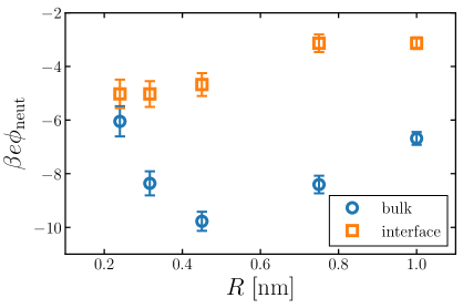
Figure 1: The average electric potential $\phi_{\rm neut}$ at the center of a neutral cavity varies considerably with the cavity’s radius $R$. Moreover, this dependence differs for the solute at $z=z_{\rm liq}$ (“bulk”) and $z=z_{\rm int}$ (“interface”). The error bars indicate 95% confidence intervals.

One strategy to remove local contributions from $\phi_{\rm neut}$ is to consider the limit $R=0$. In this extreme case the probe – in effect a neutral, non-volume excluding solute – does not break translational symmetry and induces no structural response. Given the lack of local structure, the presumably nonlocal quantity $\phi_{\rm neut}(0)=\phi_{\rm surf}$ is often called the “surface potential”. Lacking volume exclusion, however, this probe explores the liquid phase uniformly, including even the interior of solvent molecules where electrostatic potentials can be very large. A disturbing ambiguity results: The value of $\phi_{\rm surf}$ can be sensitive to modifications of a solvent model that have no impact on the solvation of any volume-excluding solute. Refs. 39 and 41 illustrate this issue vividly, constructing ‘smeared shell’ variants of SPC models with identical solvation properties but very different values of $\phi_{\rm surf}$. This variation in surface potential corresponds to differences in the so-called Bethe potential, which is discussed further in the Supporting Information (SI).

A related, and somewhat more molecular, approach to isolating the electrostatic bias from a distant phase boundary is to sum contributions to $\phi_{\rm neut}$ only from molecules that reside in the interfacial region. For a macroscopic droplet of liquid water, one could classify each molecule in a given configuration as either interfacial or bulk based on its position relative to the interface. The restricted sum

$$\phi_{\rm d}=\left\langle\sum_{j\in{\rm interface}}^{N}\sum_{\alpha}\frac{q_{\alpha}}{|{\bf r}_{j\alpha}|}\right\rangle$$ (1)

could then be considered as a macroscopically long-ranged, surface-specific component of $\phi_{\rm surf}$ that is appropriately insensitive to a solvent molecule’s internal structure. Here ${\bf r}_{j\alpha}$ denotes the position of site $\alpha$ in molecule $j$, whose charge is $q_{\alpha}$, relative to the center of the droplet. $\phi_{\rm d}$ depends significantly, however, on the way molecules are notionally divided between surface and bulk. This dependence, which has been demonstrated previously, Åqvist and Hansson (1998); Kastenholz and Hünenberger (2006) we calculate explicitly and generally in the SI. Written in the form

$$\phi_{\rm d}=-4\pi\int_{z_{\rm liq}}^{z_{\rm vap}}\!dz\,P(z)$$

where $P(z)$ is the solvent dipole density at a displacement $z$ from the interface, it reveals $\phi_{\rm d}$ as the well-known “dipole component” of the surface potential.Remsing et al. (2014); Remsing and Weeks (2019); Duignan et al. (2017a, b); Hünenberger and Reif (2011); Doyle, Shi, and Beck (2019); Horváth et al. (2013) Here, $z_{\rm liq}$ and $z_{\rm vap}$ indicate points within the bulk liquid and bulk vapor, respectively.

For SPC/E water, a surface/bulk classification in Eq. 1 based on the position of a water molecule’s center of charge gives a value $\phi_{\rm d}^{\rm center}=-40$ mV that differs from an oxygen atom-based classification, $\phi_{\rm d}^{\rm O}=240$ mV, even in sign. Because water molecules are not point particles, there is no unique way to define an interfacial population, and as a result no unique value of $\phi_{\rm d}$, though attempts have been made to define an optimal choice.Kastenholz and Hünenberger (2006) And because molecules near the liquid’s boundary are not strongly oriented on average, the range of plausible values for $\phi_{\rm d}$ is as large as their mean.

The ambiguities plaguing interpretations of $\phi_{\rm surf}$ and $\phi_{\rm d}$ are one and the same. Indeed, if we consider an interfacial population of charged sites rather than intact molecules, then $\phi_{\rm surf}$ and $\phi_{\rm d}$ become equal. (When defining an interface of intact molecules, $\phi_{\rm surf}$ and $\phi_{\rm d}$ differ by the so-called Bethe potential, whose analogous ambiguity is described in SI.) $\phi_{\rm neut}$ has been characterized as a two-interface quantity,Remsing et al. (2014); Harder and Roux (2008); Beck (2013); Arslanargin and Beck (2012); Doyle, Shi, and Beck (2019); Horváth et al. (2013) combining the bias $\phi_{\rm d}$ from the distant solvent-vapor interface together with the remaining “cavity” bias $\phi_{\rm c}=\phi_{\rm neut}-\phi_{\rm d}$ from the local solute-solvent interface. From the perspective we have described, these two interfaces are not truly separable, even if a macroscopic amount of isotropic bulk liquid intervenes between them – they must be defined consistently, and the manner of definition substantially influences the change in electrostatic potential at each interface. This is not to say that such a decomposition cannot be useful. Indeed, for computationally demanding ab initio approaches it can be convenient to consider local and nonlocal contributions to $\phi_{\rm neut}$ such that, in a first step, $\phi_{\rm c}$ can be obtained from relatively small simulations of the bulk under periodic boundary conditions. The effects of $\phi_{\rm d}$ can then be accounted for in a subsequent step involving simulations of the neat air-water interface. Such an approach was used to good effect in Ref. 30 to calculate the solvation free energy of LiF. Nonetheless, this still amounts to an arbitrary choice of dividing surface,Duignan et al. (2017a); Remsing et al. (2014); Remsing and Weeks (2019) making it challenging to assign a physical interpretation to $\phi_{\rm d}$ and $\phi_{\rm c}$ individually. Different, and equally plausible, ways of partitioning molecules can give different impressions of the two interfaces. Only the sum $\phi_{\rm neut}=\phi_{\rm c}+\phi_{\rm d}$ is unambiguous.

Establishing an absolute electrostatic bias on the bulk liquid environment due to a distant interface is thus highly problematic for water. A direct scrutiny of this nonlocal contribution, based on the fundamentally ambiguous potential $\phi_{\rm d}$, is untenable. Instead, we assess the relative importance of local and nonlocal biases by comparing the solvation properties of different ions. Local contributions can depend sensitively on features like solute size $R$ and charge $q$, while macroscopically nonlocal contributions cannot. Long-range influence of the interface might therefore be clarified by dependence of the neutral cavity potential on $R$. In particular, dominance by the distant liquid-vapor interface would imply weak variation of $\phi_{\rm neut}$ with solute size, which influences only microscopically local structure. The solute size-dependence shown in Fig. 1 does not support such a dominance. Growing the cavity from $R=0.24$ nm to $0.5$ nm lowers $\phi_{\rm neut}$ by roughly 100 mV, followed by an increasing trend for larger cavities. As emphasized in Refs. 30 and 41, the role of local charge asymmetry is far from negligible over this range of solute size.

It is tempting to expect the large-$R$ behavior of $\phi_{\rm neut}$ to reveal a strictly interfacial component, since local forces attenuate in magnitude when solvent molecules cannot approach the probe position closely. As others have noted,Remsing et al. (2014); Ashbaugh (2000) however, neutral cavities larger than $R=1$ nm induce a solvent environment with the basic character of the air-water interface.Chandler (2005) In the limit of large $R$, drying at the solute-solvent interface will generate a cavity potential that cancels the oppositely oriented distant interface with the vapor phase, yielding $\phi_{\rm neut}\approx 0$. This asymptotic cancellation should begin for nanoscale cavities, though effects of local interface curvature may cause $\phi_{\rm neut}$ to decay slowly towards zero. Judging from our results, there is no intermediate plateau value of $\phi_{\rm neut}$ that could reasonably be assigned to a single liquid-vapor interface.

I.2 Solvation thermodynamics and the asymmetry potential

The difficulty of uniquely identifying a surface dipole component of $\phi_{\rm neut}$ notwithstanding, the relevance of such neutral probe quantities for ion solvation thermodynamics has also been thoroughly examined.Duignan et al. (2017a, b); Remsing and Weeks (2016); Hummer, Pratt, and García (1996); Beck (2013); Ben-Amotz (2016); Rajamani, Ghosh, and Garde (2004); Shi and Beck (2013); Doyle, Shi, and Beck (2019); Remsing and Weeks (2019); Pollard and Beck (2016); Asthagiri, Pratt, and Ashbaugh (2003); Horváth et al. (2013); Pratt (1992) As an essential thermodynamic measure of solvation, we examine the free energy change $F_{\rm solv}(q,R)$ when a solute ion is removed from dilute vapor and added to the liquid phase. This change could be evaluated along any reversible path that transfers the solute between phases, and different paths can highlight different aspects of solvent response. For studying charge asymmetry, a particularly appealing path first creates a neutral, solute-sized cavity in the liquid, with reversible work $F_{\rm cav}(R)$. The second step, whose free energy change $F_{\rm chg}(q,R)$ was discussed above, introduces the solute’s charge.Netz and Horinek (2012) The charge asymmetry of interest compares solvating a cation and anion of the same size; since $F_{\rm cav}$ is insensitive to the solute’s charge, its contribution to $F_{\rm solv}=F_{\rm cav}+F_{\rm chg}$ cancels in the difference

$$F_{\rm solv}(q,R)-F_{\rm solv}(-q,R) = F_{\rm chg}(q,R)-F_{\rm chg}(-q,R)$$ (2)

$$\equiv 2q\psi(q,R)$$ (3)

Eq. 3 defines an asymmetry potential $\psi$, an analogue of $\phi_{\rm neut}$ that accounts for solvent response.

The connection between $\psi(q,R)$ and $\phi_{\rm neut}$ can be made precise through a cumulant expansion of $F_{\rm chg}$ in powers of $q$,Kubo (1962); Hummer, Pratt, and García (1996); Beck (2013); Ben-Amotz (2016); Rajamani, Ghosh, and Garde (2004)

$$F_{\rm chg}(q,R)=q\langle\phi_{\rm solv}\rangle_{0}-\frac{\beta q^{2}}{2}\langle(\delta\phi_{\rm solv})^{2}\rangle_{0}+\mathcal{O}(q^{3}),$$ (4)

where $\langle\cdots\rangle_{0}$ denotes a canonical average in the presence of a neutral solute-sized cavity, $\phi_{\rm solv}$ is the fluctuating electric potential at the center of the cavity due to the surrounding solvent (so that $\phi_{\rm neut}=\langle\phi_{\rm solv}\rangle_{0}$), and $\delta\phi_{\rm solv}=\phi_{\rm solv}-\phi_{\rm neut}$. The $\mathcal{O}(q^{2})$ term in Eq. 4 describes linear response of the solvent potential $\phi_{\rm solv}$ to the solute’s charging. This response, which could be captured by a Gaussian field theory à la DCT, is charge symmetric by construction. The asymmetry potential $\psi(q,R)=\phi_{\rm neut}(R)+\mathcal{O}(q^{2})$ is therefore equivalent to $\phi_{\rm neut}$ within linear response.

Previous work has demonstrated that water’s response to charging sub-nanometer cavities is significantly nonlinear.Remsing and Weeks (2016); Bardhan, Jungwirth, and Makowski (2012); Hummer, Pratt, and García (1996); Lynden-Bell and Rasaiah (1997); Cox and Geissler (2018); Shi and Beck (2013); Hirata, Redfern, and Levy (1988); Grossfield (2005); Duignan et al. (2017b); Loche et al. (2018) In $\psi(q,R)$ the breakdown of linear dielectric behavior is evidenced by deviations away from the limiting value $\psi(0,R)=\phi_{\rm neut}(R)$. Fig. 2a shows our numerical results for the asymmetry potential as a function of $q$ for solutes in bulk liquid SPC/E water. For large solutes ($R\gtrsim 0.5$ nm), the variation of $\psi$ is modest as $q$ increases from 0 to $e$. For smaller cavities, linear response theory fails dramatically, in that charge asymmetry changes many-fold as the solute is charged. In the case of a fluoride-sized solute, the asymmetry at full charge ($e\psi(e,R_{\rm F})\approx 26k_{\rm B}T$) is qualitatively different than in linear response ($e\phi_{\rm neut}(R_{\rm F})\approx-8k_{\rm B}T$). For SPC models of bulk liquid water, the ultimate electrostatic bias in solvating cations and anions of this size clearly cannot be attributed to the innate environment of a neutral cavity, much less to the structure of a distant interface. Ab initio molecular dynamics studies have reached a similar conclusion.Duignan et al. (2017b)

SPC simulations of bulk liquid water indicate that the nonlinearity of solvent response to solute charging has a step-like character:Hummer, Pratt, and García (1996); Lynden-Bell and Rasaiah (1997); Bardhan, Jungwirth, and Makowski (2012) For one range of solute charge ($q<q_{\rm c}$), the susceptibility $d\langle\phi_{\rm solv}\rangle_{q}/dq$ is approximately constant. In the remaining range ($q\geq q_{\rm c}$), $d\langle\phi_{\rm solv}\rangle_{q}/dq$ is also nearly constant, but with a different value. Piecewise linear response (PLR) models inspired by this observation give a broadly reasonable description of bulk solvation thermodynamics throughout the entire range $-e<q<+e$. In our discussion of ion adsorption below, we will assess the suitability of a PLR model for interfacial solvation as well.

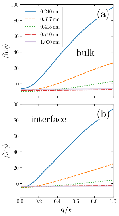
Figure 2: Ion solvation in water is both asymmetric and non-linear, as quantified by the asymmetry potential $\psi(q,R;z)$. Results are shown for solutes (a) in the bulk liquid, and (b) near the air-water interface, spanning ranges of charge $0<q\leq e$ and solute size $0.24\leq R\leq 1.0$ nm (see legend). Both in the bulk and at the interface, $\psi<0$ for small $q$, indicating that weakly charged cations are more favorably solvated than anions. For the smaller solutes, $\psi$ increases with $q$, a signature of non-linear response. Anions consequently become more favorably solvated at large $q$. For the larger solutes ($R=0.75$ nm and $R=1.0$ nm) the solvent response is approximately linear, as reflected by the weak dependence of $\psi$ on $q$.

II Charge asymmetry in ion adsorption

In bulk liquid water, an electric potential from its bounding interfaces cannot be unambiguously identified. Even the sign of the bias generated by a liquid-vapor interface is unclear. Moreover, the nonlinear local response to solute charging can exert a bias on ion solvation that significantly outweighs the charge asymmetry due to distant interfaces.

Solvation within the interfacial environment is hardly less complex, juxtaposing the fluctuating intermolecular arrangements of bulk water together with broken symmetry and the microscopic shape variations of a soft boundary. It is thus unlikely that complications described in Sec. I for bulk liquid are much eased in the interfacial scenario. We should not expect, for example, that the neutral cavity potential for a solute positioned near the interface will be dominated by a simple nonlocal contribution. Nor should we expect the accuracy of linear response approximations to be greatly improved, such that $\phi_{\rm neut}$ is predictive of charge asymmetric solvation.

The adsorption of an ion to the interface, however, concerns the difference in solvation properties of bulk and interfacial environments. To the extent that nonlinear response and local structuring at the interface are similar to those in bulk liquid, their effects may cancel, or at least significantly offset, in the thermodynamics of adsorption. Our main results concern this possibility of cancellation, which would justify regarding macroscopically nonlocal contributions to $\phi_{\rm neut}$ as the basic origin of charge asymmetry in ion adsorption.

We begin by establishing that biases on solvation at the interface are complicated in ways that qualitatively resemble biases in bulk. As before, we consider solutes with a range of sizes and charges, now positioned at the liquid’s boundary (illustrated in Fig. 3a). The free energies and potentials defined in Sec. I for bulk solution now acquire dependence on the Cartesian coordinate $z$ that points perpendicular to the mean surface. SI shows the detailed location $z_{\rm int}$ we designate as adsorbed for each ion. In all cases $z_{\rm int}$ lies near the Gibbs dividing surface, where the solvent density falls to half its bulk value. The larger solutes occupy considerable volume, so that the solvent density profile in our finite simulation cell changes noticeably with their height $z$. A precise interfacial solute location is therefore difficult to justify. When neutral and located near $z_{\rm int}$, however, these nanometer-size solutes tend to deform the instantaneous phase boundary,Willard and Chandler (2010); Vaikuntanathan and Geissler (2014); Vaikuntanathan et al. (2016) just as they induce local drying in bulk solution.Chandler (2005) This response essentially fixes their location relative to the instantaneous interface, so that their solvation properties should be fairly insensitive to the choice of $z_{\rm int}$.

The neutral cavity potential for interfacial solutes is shown in Fig. 1. As was observed for the bulk liquid, $\phi_{\rm neut}$ is consistently negative over the range $R=0.24$ nm to $R=1$ nm but varies significantly with solute size. In this case the potential increases nearly monotonically with $R$, though the values of $\phi_{\rm neut}(0.75\,{\rm nm})$ and $\phi_{\rm neut}(1\,{\rm nm})$ are statistically indistinguishable within our sampling. Just as for bulk liquid, we expect $\phi_{\rm neut}$ to vanish in the limit $R\rightarrow\infty$. Here, drying at the surface of very large solutes effects a distortion of the liquid-vapor interface that places the probe (located at the cavity’s center) distinctly in the vapor phase. Judging from our results, the asymptotic approach to this limit is quite slow for interfacial solutes. Nonetheless, $\phi_{\rm neut}$ changes by nearly 40% over the range of $R$ considered, emphasizing the importance of local, solute-dependent contributions. As concluded for the bulk solvent, macroscopically nonlocal potentials arising from orientational structure of the air-water interface do not dominate the charge asymmetry experienced by neutral solutes at $z_{\rm int}$.

The response to charging a solute at the air-water interface is strongly nonlinear, to a degree comparable with bulk response. A similarly important role of nonlinear response at interfaces has been reported previously.Loche et al. (2018); Noah-Vanhoucke and Geissler (2009) The resulting $q$-dependent charge asymmetry closely resembles bulk behavior, as quantified by the asymmetry potential $\psi(q,R;z)$, whose dependence on solute position we now make explicit. Fig. 2b shows simulation results for $\psi(q,R;z_{\rm int})$ for SPC/E water. On the scale that $\psi$ changes as $q$ increases from 0 to $e$, the charging response in bulk liquid and at the interface are nearly indistinguishable by eye. This close similarity suggests that the predominant source of nonlinearity lies in aspects of local response which are not so different in the two environments.

Comparing $\psi(q,R;z_{\rm int})$ with $\psi(q,R;z_{\rm liq})$, and $\phi_{\rm neut}(R;z_{\rm int})$ with $\phi_{\rm neut}(R;z_{\rm liq})$, gives a sense for features of solvation that most strongly shape ion adsorption. Similarities point to aspects of solvent structure and response which are largely unchanged when an ion moves to the interface. These contributions may be important for solvation in an absolute sense, but their cancellation indicates a weak net influence on adsorption thermodynamics.

For all values of $R$ we considered, $\phi_{\rm neut}$ is less negative at $z_{\rm int}$ than at $z_{\rm liq}$. In the simplest conception of the liquid’s boundary as a layer of nonzero dipole density, one would expect the nonlocal component of $\phi_{\rm neut}$ to attenuate steadily in magnitude as a solute moves from the liquid phase into the interfacial region, and then vanish as the solute enters vapor. Whether this rough picture is consistent with the observed shift in $\phi_{\rm neut}$ depends on the sign of the nonlocal potential $\phi_{\rm d}$. Unfortunately this sign is uncertain, as described in Sec. I, due to the intrinsic ambiguity in dividing molecules between bulk and surface regions. Ref. 41 calculated a positive dipole component of the surface potential, $\phi_{\rm d}=+260$ mV. Within the simple continuum picture, this value suggests a downward shift in $\phi_{\rm neut}$ as $z$ increases from $z_{\rm liq}$ to $z_{\rm int}$, in contrast to our simulation results. A different partitioning scheme, however, can give $\phi_{\rm d}<0$, suggesting an upward shift, as we observe in simulation.

Although the direction of change in $\phi_{\rm neut}$ might be anticipated from the sign of $\phi_{\rm d}$, the magnitude of this shift varies considerably with solute size. For $R=0.24$ nm, $|\phi_{\rm neut}|$ is reduced by about 15% when the cavity is placed at the interface. For $R=0.415$ nm the reduction is greater than 50%. This variation cannot arise from nonlocal biases, which are insensitive to the size or charge of a solute. A distinct, macroscopically nonlocal contribution could manifest as a nonzero asymptotic value of $\Delta_{\rm ads}\phi_{\rm neut}=\phi_{\rm neut}(R;z_{\rm int})-\phi_{\rm neut}(R;z_{\rm liq})$ at intermediate $R$; according to our data, if such a limit exists it occurs for solutes larger than 1 nm.

The similarity between the asymmetry potentials $\psi(q,R)$ for solutes in the bulk and at the interface offers some hope that complicating factors of nonlinear response cancel out in the adsorption process. The extent of this cancellation is quantified by an adsorption asymmetry potential

$$\Delta_{\rm ads}\psi(q,R) =\psi(q,R;z_{\rm int})-\psi(q,R;z_{\rm liq}),$$ (5)

$$=(2\beta q)^{-1}\ln{\left[{\rho_{\rm int}(-q,R;\rho_{\rm bulk})\over\rho_{\rm int}(+q,R;\rho_{\rm bulk})}\right]},$$ (6)

where $\rho_{\rm int}$ is the average number density of a solute at $z=z_{\rm int}$, given its concentration $\rho_{\rm bulk}$ in bulk solution. Eq. 6 highlights the direct relationship between $\Delta_{\rm ads}\psi(q,R)$ and the relative adsorption propensities of cations and anions: For dilute solutes with opposite charge, equal size, and equal bulk concentration, $\exp{[2\beta q\Delta_{\rm ads}\psi(q,R)]}$ directly indicates the enhancement of anions over cations at the interface, as shown in Figs. 3 and 4. From the preceding discussion of the asymmetry potential itself, it is clear that $\Delta_{\rm ads}\psi(q\to 0,R)=\Delta_{\rm ads}\phi_{\rm neut}$. The full dependence of $\Delta_{\rm ads}\psi$ on $q$ thus incorporates the adsorption behavior of the neutral cavity potential as well as the corresponding solvent response to charging. Our numerical results for $\Delta_{\rm ads}\psi(q,R)$ are the central contribution of this paper.

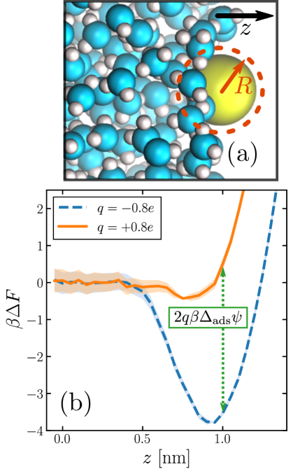
Figure 3: The propensity for an ion to adsorb to the air-water interface depends strongly on the sign of its charge. (a) Snapshot of an iodide-sized anion ($R=0.415$ nm) at the interface. The system comprises a free-standing slab of liquid water surrounded on either side by its vapor. (Only one of the two interfaces is shown.) The $z$ direction is indicated by the arrow. The size of the solute is depicted schematically by the dashed circle. (b) Potential of mean force $\Delta F$ as a function of ion position $z$, for a solute charge $q=+0.8e$ (solid orange) and $q=-0.8e$ (dashed blue). The anion adsorbs much more strongly to the interface than the cation for this solute size. The dotted green line indicates the connection between these free energy profiles and the adsorption asymmetry potential in Eq. 6.

The adsorption asymmetry potential $\Delta_{\rm ads}\psi(q,R)$, as determined from simulations of the SPC/E model, are plotted as a function of $q$ in Fig. 4 for several values of $R$. For the smaller solutes, the scale on which $\Delta_{\rm ads}\psi$ changes upon charging is dramatically smaller than the asymmetry potentials themselves. Nonlinear solvent response in these cases cancels substantially in the process of adsorption, but by no means completely. Despite the partial cancellation, $\Delta_{\rm ads}\psi$ still varies by more than 100 mV as $q$ increases from 0 to $e$, comparable in magnitude to $\phi_{\rm d}$ and $\phi_{\rm neut}$. For $R=0.24$ nm and $R=0.317$ nm, this variation is sufficient to change even the sign of $\Delta_{\rm ads}\psi$, and therefore to change the sense of charge bias: Small monovalent cations “adsorb” more favorably to the air-water interface than do anions of the same size. In this size range, however, the adsorbed state is unstable relative to the fully solvated ion in bulk solvent unless $q$ is very small in magnitude.

As was previously observed for bulk solvation, we find that the response to charging a solute at the air-water interface, while nonlinear on the whole, is roughly piecewise linear. Deviations from piecewise linearity are generally stronger in the interfacial case. It is therefore less straightforward to parameterize an interfacial piecewise linear response model, i.e., to identify a crossover charge $q_{\rm c}$ at which the susceptibility $d\langle\phi_{\rm solv}\rangle_{q}/dq$ changes discontinuously. The SI presents plausible choices for $q_{\rm c}$ and these limiting susceptibilities for our three smallest solutes, from which adsorption asymmetry potentials $\Delta_{\rm ads}\psi^{\rm(PLR)}$ can be readily computed. The resulting PLR predictions are plotted in Fig. 4b. Two basic features of our simulation results are accurately captured by this phenomenological description. Specifically, (i) for small solute charge, $\Delta_{\rm ads}\psi$ is an approximately constant or modestly increasing function of $q$, and (ii) a more strongly decreasing trend of $\Delta_{\rm ads}\psi$ follows for larger $q$. Nearly quantitative agreement can be obtained for an iodide-sized solute, $R=0.415$ nm. Smaller solutes exhibit a more complicated charge dependence that lies beyond a simple PLR description. We note that this test of PLR is a demanding one, given the small scale of $\Delta_{\rm ads}\psi$ relative to $\psi(q,R;z_{\rm int})$ and $\psi(q,R;z_{\rm liq})$ individually. To the extent that PLR is a successful caricature, these results suggest that the adsorption charge asymmetry at full charging ($q=e$) derives from a combination of features of solvent response, including an interface-induced shift in the crossover charge $q_{\rm c}$ at which the character of linear response changes. The neutral cavity potential $\phi_{\rm neut}$ figures into this combination as well, but by no means does it dominate for these solute sizes.

For the larger solutes we examined, the nonlinearity of solvent response to charging is not pronounced, either in bulk liquid or at the interface. The difference in nonlinearity of these environments is necessarily also not large, with $e\Delta_{\rm ads}\psi$ changing by less than $k_{\rm B}T$ over the range $q=0$ to $q=e$. This small variation is comparable in scale to those of $\psi(q,R;z_{\rm int})$ and $\psi(q,R;z_{\rm liq})$ themselves. Judged on that scale, the cancellation of nonlinear response is in fact less complete for $R=0.75$ nm than for smaller solutes. As we have discussed, cavities with $R\gtrsim 1$ nm depress the instantaneous interface significantly, effectively placing them in the vapor phase even when $z$ coincides with the Gibbs dividing surface. When such a solute is endowed with sufficient charge, wetting will occur at its surface, eventually raising the interface to effectively move the solute into the liquid phase. This solvent response, which originates in the physics of phase separation, is intrinsically nonlinear. For large $R$, a solute charge well in excess of $e$ is required to fully induce this structural change, but at the nanoscale it may manifest as an incipient nonlinearity for $q\approx e$.

In summary, the adsorption asymmetry potential $\Delta_{\rm ads}\psi$ depends significantly on solute size $R$ and charge $q$. Neither of these sensitivies can arise from intrinsic orientational bias at the neat air-water interface. Long-range electrostatic forces from oriented molecules at the liquid’s boundary, which contribute importantly to surface potentials like $\phi_{\rm surf}$ and $\phi_{\rm d}$, are inherently unaffected by the presence, size, or charge of a sufficiently distant solute. These results highlight the importance of local solvent structure and response for charge asymmetry in interfacial ion adsorption, and they highlight the danger of inferring solvation thermodynamics from ion-free quantities such as $\phi_{\rm surf}$ and $\phi_{\rm d}$.

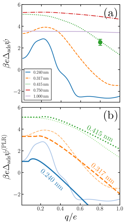
Figure 4: Linear response theory cannot faithfully describe the differences between adsorption profiles of sub-nanometer anions and cations, as demonstrated in (a) by variations in adsorption asymmetry potential $\Delta_{\rm ads}\psi$ with both $R$ and $q$. For the smallest solutes ($R\lesssim 0.4$ nm), $\Delta_{\rm ads}\psi$ even changes sign as $q$ increases. In this size range, fully charged cations are more abundant at the interface than anions (with the same bulk concentration). At larger $R$, solutes with $q=-e$ adsorb more strongly than those with $q=+e$. As the solute diameter approaches $R=1$ nm, nonlinear response during the charging process becomes much less pronounced. Values of $R$ are indicated in the legend. (b) A PLR model (heavy lines) predicts $\Delta_{\rm ads}\psi$ is initially flat, followed by a steady decrease as $q$ increases. This qualitatively captures the simulation data (light lines), although it fails to capture the leveling off at large $q$ seen for $R=0.240$ nm and $0.317$ nm.

III Discussion and Conclusions

In this study, we set out to understand whether or not charge asymmetry in interfacial ion adsorption could be understood in terms of macroscopically long-ranged, collective forces intrinsic to water. For ion solvation in bulk, difficulties in unambiguously determining such long-ranged contributions were already apparent from previous results. Building on that work, our results show that for SPC models of water such a simple mechanistic picture is inadequate for interfacial solvation as well. In addition to the difficulties in partitioning molecules between ‘near’ and ‘distant’ interfaces, complex nonlinear response also underlies substantial shortcomings of trying to rationalize ion adsorption from surface potentials that characterize biases of the undisturbed air-water interface. The nonlinearities in $F_{\rm chg}(q,R)$ for bulk and interfacial environments, while similar, are sufficiently different that the process of adsorption is also substantially nonlinear. A compelling inference of adsorption tendencies from intrinsic properties of the undisturbed liquid and its interface with vapor requires information that is more subtle than an average electric potential and macroscopic dielectric susceptibility. As highlighted by the potential distribution theorem,Widom (1982) this information can in principle be gleaned from equilibrium statistics of the undisturbed solvent. But in terms of fluctuations in electric potential, it involves high-order correlations whose physical meaning is not transparent.

In previous work we developed and tested finite size corrections for computer simulations of interfacial ion solvation.Cox and Geissler (2018) Based on DCT, these corrections proved to be quite accurate even for simulation unit cells with nanometer dimensions. Our conclusion that DCT is a faithful representation of aqueous polarization response down to nanometer length scales is reinforced by the results of this paper. In particular, when charging a solute of diameter $R=1$ nm, solvent response on an absolute scale is linear to a very good approximation, both in bulk liquid and at the interface. The results of Figs. 2 and 4, however, also indicate that 1 nm marks the validity limit of linear response. When charging a cavity with $R=0.75$ nm, nonlinear contributions to charge asymmetry are quantitatively important; for smaller solutes such nonlinear contributions become not just important but instead dominant. In passing, we note that even for the larger solutes, a significant charge asymmetry persists, both for bulk solvation and for adsorption to the interface. This persistent bias weighs against the basis of the tetra-phenyl arsonium/tetra-phenyl borate (‘TATB’) extrathermodynamic assumption, an issue that has also been raised by others.Duignan, Baer, and Mundy (2018); Pollard and Beck (2018); Scheu et al. (2014); Remsing and Weeks (2019)

The highly simplified description of molecular interactions in SPC models is certainly a crude approximation to real microscopic forces. But the specific ion effects it exhibits cannot be ascribed simply to an errant surface potential. Indeed, discrepancies between models in potentials such as $\phi_{\rm d}$ (whose definition requires an arbitrary convention), $\phi_{\rm surf}$ (which pertains to a solute that does not exclude volume), or even $\phi_{\rm neut}$ (which for subnanometer solutes does not account for the strong asymmetry of solvent response) are not greatly alarming. $\phi_{\rm surf}$ and $\phi_{\rm d}$ can vary significantly among different models, but they do not weigh on ion solvation thermodynamics in a direct way, either in bulk liquid or at the air-water interface. (This does not contradict their use for computing $F_{\rm chg}$ once a choice for partitioning molecules between the interface and bulk has been made.) By contrast, trends in $F_{\rm solv}$ and $\Delta_{\rm ads}\psi$ at full charging reflect on essential microscopic mechanisms that underlie specific ion adsorption. SPC models may be best viewed as caricatures of a disordered tetrahedral network, with intrinsic charge asymmetry due to the distinct geometric requirements of donating and accepting hydrogen bonds. These essential features of liquid water are often associated with nonlinear response in solvation.Maroncelli and Fleming (1988); Skaf and Ladanyi (1996); Geissler and Chandler (2000) By implicating nonlinearities of precisely this kind as sources of ion-specific adsorption properties, our results support the use of SPC models as a physically motivated test bed for exploring the microscopic basis of surprising trends in interfacial solvation. Conversely, our results underscore the limitations of DCT and notions of long-ranged contributions from unperturbed interfaces, which do not describe essential local aspects of the chemical physics underlying ion adsorption and its charge asymmetry. The consequences of this shortcoming are likely to be exacerbated in confined geometries. Work to move beyond standard DCT approaches is an active area of research (e.g. Refs. 24; 25; 26; 69) and it is hoped that the results presented in this study will help to guide future theoretical developments.

IV Methods

All simulations used the SPC/E water model;Berendsen, Grigera, and Straatsma (1987) solutes were represented as Lennard-Jones (LJ) spheres with a central charge $q$. The SHAKE algorithm was used to maintain a rigid water geometry.Ryckaert, Ciccotti, and Berendsen (1977) Periodic boundary conditions were imposed in all three Cartesian directions, with the liquid phase spanning two directions in a slab geometry. Long-range Coulomb interactions were summed using the particle-particle particle-mesh Ewald method.Hockney and Eastwood (1988); Kolafa and Perram (1992) A spatially homogeneous background charge was included to maintain electroneutrality and thus guarantee finite electrostatic energy. For solute sizes $R<0.75$ nm, the system comprised 266 water molecules with simulation cell dimensions $2\times 2\times 4.5$ nm³. For $R\geq 0.75$ nm the simulation cell size was $3.5\times 3.5\times 8.5$ nm³ and we used 1429 water molecules. Solvent density profiles that indicate the interfacial location $z_{\rm int}$ for each solute are given in the SI. A time step of 1 fs was used for all simulations. A temperature of 298 K was maintained using Langevin dynamics,Dünweg and Paul (1991); Schneider and Stoll (1978) as implemented in the LAMMPS simulation package,Plimpton (1995) which was used throughout.

Due to the long range of Coulomb interactions, ion solvation in polar solvents has important contributions even from distant solvent molecules. Thermodynamic estimates from molecular simulations are thus subject to substantial finite size effects, which have been the focus of many studies.Hummer, Pratt, and García (1996); Figueirido, Del Buono, and Levy (1997); Hummer, Pratt, and García (1997); Hünenberger and McCammon (1999); Hummer, Pratt, and García (1998) In Ref. 37 we showed for liquid water in a periodic slab geometry that values of $\phi_{\rm neut}$ depend on simulation box size in a slowly decaying but predictable way. The limit of infinitely separated periodic images can thus be obtained with a simple finite size correction, which amounts to referencing electric potential values to the vapor phase. We have applied this correction to all potentials reported in this paper. The potential of mean force $\Delta F(q,R;z)$ for ions in periodic liquid slabs are, by contrast, nearly independent of simulation cell size for $z\leq z_{\rm int}$.Cox and Geissler (2018)

To compute $\Delta F(q,R;z)$, we followed the same procedure as outlined in Ref. 18, namely umbrella sampling and histogram reweighting with MBAR.Shirts et al. (2007) To calculate $\psi(q,R;z)$ for a given choice of $R$ and $z$, simulations were performed with $q/e=-1.0,-0.9,\ldots,+0.9,\textrm{ and }+1.0$. This spacing of $q$ values allows for ample overlap among probability distributions $P_{q}\big{(}\phi_{\rm solv}\big{)}$ of the electrostatic potential at the center of the solute (Fig. S10). For $R\leq 0.415$ nm statistics were obtained from trajectories 5 ns in duration. For $R=0.75$ nm and $1.0$ nm, trajectories varied between $2.8$ ns and $5.0$ ns. Using the MBAR algorithm, results from the entire range of solute charge were combined to determine the neutral cavity distribution $P_{0}(\phi_{\rm solv})$ over a correspondingly broad range of $\phi_{\rm solv}$. $F_{\rm chg}$ was computed by averaging $\exp(-\beta q\phi_{\rm solv})$ according to the distribution $P_{0}(\phi_{\rm solv})$, as prescribed by Widom’s potential distribution theorem,Widom (1982)

$$e^{-\beta F_{\rm chg}}=\int\!\mathrm{d}\phi_{\rm solv}\,P_{0}\big{(}\phi_{\rm solv}\big{)}e^{-\beta q\phi_{\rm solv}}$$ (7)

The integral in Eq. 7 was performed numerically.

Supporting Information

This document contains a detailed account of the issues faced when trying to isolate contributions to $\phi_{\rm neut}$ from local and distant sources. Also given are solvent density profiles $\rho(z)$ in the presence of the neutral solute for the different systems studied, and the position of the solute at the interface is indicated in each instance. Solute-solvent radial distribution functions $g(r)$ are shown for $q=-e$, $0$ and $+e$ with the solute in the center of the slab. Details underlying the piecewise linear response model are also presented. A brief description of how $P_{0}(\phi_{\rm solv})$ is obtained is given.

S1 Electrostatic contributions from near and far

The challenge of identifying and interpreting a potential drop across the liquid-vapor interface can be viewed as an issue of partitioning molecules between distinct regions of space.

Consider a macroscopic droplet of liquid bounded by an interface $S$ with the vapor phase (as illustrated in Fig. S1). The origin of our coordinate system lies deep within the bulk liquid phase. We will aim to calculate the average electric potential $\langle\phi\rangle$ at the origin, distinguishing contributions of molecules that are far from the probe (including those at the phase boundary) from those that lie nearer the origin. Specifically, we will divide the two populations at an imaginary surface $B$ that is also deep within the bulk liquid. We will take $B$ to be distant enough from the origin that liquid structure on this surface is bulk in character, even if the microscopic vicinity of the origin is complicated by a solute’s excluded volume.

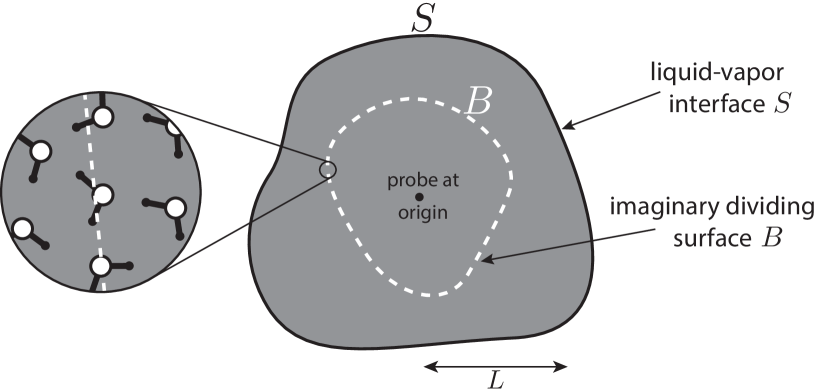
Figure S1: Sketch of a macroscopic droplet of liquid (shaded region at right) surrounded by dilute vapor. The two phases contact at a macroscopically smooth interface $S$. The surface $B$ within the droplet is a mathematical device to isolate the electrostatic contribution of molecules residing near the phase boundary $S$. The droplet’s overall scale $L$ is a macroscopic distance. A magnified view of a microscopic region straddling $B$ is shown at left. Molecules intersected by $B$ (dashed white line) could reasonably be assigned to either the near (inside $B$) or far (outside $B$) domains.

S1.1 Partitioning schemes

The vast majority of molecules in the droplet are unambiguously located either outside $B$ (“far”) or inside $B$ (“near”). A tiny fraction straddle the surface $B$. In the case of water this could involve a molecule’s oxygen atom lying on one side of $B$, while its hydrogen atoms lie on the other. One division scheme (an M-scheme) would judge the molecule’s location based on the O atom; another M-scheme might base the classification on the molecule’s center of charge. A still different scheme (a P-scheme) could divide the molecule in two, with some pieces “near” and other pieces “far”. (The M-scheme and the P-scheme are well known in the literature. See e.g. Ref. Kastenholz and Hünenberger, 2006.) The total potential $\phi$ at the probe site is not sensitive to which of these schemes is chosen. But its contributions $\phi_{\textrm{near}}$ and $\phi_{\textrm{far}}$ from atoms/molecules in the near and far regions are sensitive, in an offsetting way.

Let’s first treat the M scheme, with the molecule’s near/far classification based on the position $\mathbf{r}^{(0)}$ of some site within the molecule (say, its O atom). The average far-field potential in this case is

$$\langle\phi_{\textrm{far}}^{\textrm{M}}\rangle=N\int_{\textrm{outside $B$}}d\mathbf{r}\int d\mathbf{\Omega}\,p(\mathbf{r},\mathbf{\Omega})\sum_{\alpha}{q_{\alpha}\over|\mathbf{r}+\Delta\mathbf{r}_{\alpha}(\mathbf{\Omega})|},$$ (S1)

where $N$ is the total number of molecules in the droplet and $\alpha$ indexes charged sites within each molecule. Here, $p(\mathbf{r},\mathbf{\Omega})=\langle\delta(\mathbf{r}-\mathbf{r}^{(0)})\delta(\mathbf{\Omega}-\mathbf{\Omega}^{(0)})\rangle$ is the joint probability distribution of a molecule’s position (i.e., $\mathbf{r}^{(0)}$) and intramolecular configuration $\mathbf{\Omega}^{(0)}$ (specified relative to the reference position $\mathbf{r}^{(0)}$, as indicated by the superscript). By $\Delta\mathbf{r}_{\alpha}=\mathbf{r}_{\alpha}-\mathbf{r}^{(0)}$ we denote the displacement of charge $q_{\alpha}$ from the reference point $\mathbf{r}^{(0)}$. This intramolecular displacement is entirely determined by $\mathbf{\Omega}^{(0)}$.

For the P-scheme, each charge $\alpha$ contributes to $\phi_{\textrm{far}}^{\textrm{P}}$ if $\mathbf{r}_{\alpha}$ lies outside $B$. The corresponding far-field potential is

$$\langle\phi_{\textrm{far}}^{\textrm{P}}\rangle = N\sum_{\alpha}\int_{\textrm{outside $B$}}d\mathbf{r}\int d\mathbf{\Omega}\,p_{\alpha}(\mathbf{r},\mathbf{\Omega}){q_{\alpha}\over|\mathbf{r}|}$$ (S2)

$$= N\sum_{\alpha}\int_{\textrm{outside $B$}}d\mathbf{r}\int d\mathbf{\Omega}\,p(\mathbf{r}-\Delta\mathbf{r}_{\alpha},\mathbf{\Omega}){q_{\alpha}\over|\mathbf{r}|}$$ (S3)

where $p_{\alpha}(\mathbf{r},\mathbf{\Omega})$ is the joint probability distribution for site position $\mathbf{r}_{\alpha}$ and intramolecular configuration of a solvent molecule. In Eq. S3 we have made use of the connection

$$p_{\alpha}(\mathbf{r},\mathbf{\Omega}) = \langle\delta(\mathbf{r}-\mathbf{r}_{\alpha})\delta(\mathbf{\Omega}-\mathbf{\Omega}^{(0)})\rangle=\langle\delta(\mathbf{r}-\Delta\mathbf{r}_{\alpha}-\mathbf{r}^{(0)})\delta(\mathbf{\Omega}-\mathbf{\Omega}^{(0)})\rangle$$ (S4)

$$= p(\mathbf{r}-\Delta\mathbf{r}_{\alpha}(\mathbf{\Omega}),\mathbf{\Omega})$$ (S5)

between the distributions $p$ and $p_{\alpha}$.

S1.2 Multipole expansion

Since the entire “far” region is macroscopically distant from the origin, small-$\Delta\mathbf{r}_{\alpha}$ expansions of $|\mathbf{r}+\Delta\mathbf{r}_{\alpha}|^{-1}$ and $p(\mathbf{r}-\Delta\mathbf{r}_{\alpha},\mathbf{\Omega})$ are well justified. These yield

$$\sum_{\alpha}{q_{\alpha}\over|\mathbf{r}+\Delta\mathbf{r}_{\alpha}|}=\left(\sum_{\alpha}q_{\alpha}\Delta\mathbf{r}_{\alpha}\right)\cdot\nabla{1\over r}+{1\over 2}\left(\sum_{\alpha}q_{\alpha}\Delta\mathbf{r}_{\alpha}\Delta\mathbf{r}_{\alpha}\right):\nabla\nabla{1\over r}+\ldots$$ (S6)

and

$$\sum_{\alpha}q_{\alpha}p(\mathbf{r}-\Delta\mathbf{r}_{\alpha},\mathbf{\Omega})=-\nabla\cdot\sum_{\alpha}q_{\alpha}\Delta\mathbf{r}_{\alpha}p(\mathbf{r},\mathbf{\Omega})+{1\over 2}\nabla\nabla:\sum_{\alpha}q_{\alpha}\Delta\mathbf{r}_{\alpha}\Delta\mathbf{r}_{\alpha}p(\mathbf{r},\mathbf{\Omega})+\ldots$$ (S7)

where we have omitted leading terms proportional to $\sum_{\alpha}q_{\alpha}$, which vanish by molecular charge neutrality. When carried through subsequent calculations, terms beyond quadrupole order in these expansions would vanish due either to symmetry or to the macroscopic scale of the droplet.

Defining dipole and quadrupole densities as

$$\mathbf{m}(\mathbf{r})=N\int d\mathbf{\Omega}\,p(\mathbf{r},\mathbf{\Omega})\sum_{\alpha}q_{\alpha}\Delta\mathbf{r}_{\alpha}$$ (S8)

and

$$\mathbf{Q}(\mathbf{r})={N\over 2}\int d\mathbf{\Omega}\,p(\mathbf{r},\mathbf{\Omega})\sum_{\alpha}q_{\alpha}\Delta\mathbf{r}_{\alpha}\Delta\mathbf{r}_{\alpha}$$ (S9)

we can write

$$\langle\phi_{\textrm{far}}^{\textrm{M}}\rangle=\int_{\textrm{outside $B$}}d\mathbf{r}\left(\mathbf{m}(\mathbf{r})\cdot\nabla{1\over r}+\mathbf{Q}(\mathbf{r}):\nabla\nabla{1\over r}+\ldots\right)$$ (S10)

and

$$\langle\phi_{\textrm{far}}^{\textrm{P}}\rangle=\int_{\textrm{outside $B$}}d\mathbf{r}{1\over r}\left(-\nabla\cdot\mathbf{m}(\mathbf{r})+\nabla\nabla:\mathbf{Q}(\mathbf{r})+\ldots\right)$$ (S11)

Integrating by parts, and noting that $\mathbf{m}(\mathbf{r})$ and $\nabla:\mathbf{Q}(\mathbf{r})$ vanish both on $B$ and at infinity,

$$\langle\phi_{\textrm{far}}^{\textrm{P}}\rangle = \int_{\textrm{outside $B$}}d\mathbf{r}\left(\mathbf{m}(\mathbf{r})\cdot\nabla{1\over r}-\left(\nabla{1\over r}\right)\cdot\big{(}\nabla\cdot\mathbf{Q}(\mathbf{r})\big{)}\right)$$ (S12)

$$= \int_{\textrm{outside $B$}}d\mathbf{r}\left(\mathbf{m}(\mathbf{r})\cdot\nabla{1\over r}-\nabla\cdot\left(\nabla{1\over r}\cdot\mathbf{Q}(\mathbf{r})\right)+\mathbf{Q}(\mathbf{r}):\nabla\nabla{1\over r}\right)$$ (S13)

Using the divergence theorem,

$$\langle\phi_{\textrm{far}}^{\textrm{P}}\rangle=\langle\phi_{\textrm{far}}^{\textrm{M}}\rangle-\int_{B}d\mathbf{R}\,\,\hat{\mathbf{n}}(\mathbf{R})\cdot\left(\nabla{1\over R}\cdot\mathbf{Q}(\mathbf{R})\right)$$ (S14)

where $\mathbf{R}$ is a point on $B$ and $\hat{\mathbf{n}}(\mathbf{R})$ is the corresponding local inward-pointing normal vector. Since $B$ lies within the bulk liquid, where the average quadrupole density $\mathbf{Q}_{\textrm{liq}}$ is isotropic, $\mathbf{Q}(\mathbf{r})=\mathbf{I}\,(\textrm{Tr}\mathbf{Q}_{\textrm{liq}}/3)$ everywhere on this surface. As a result,

$$\langle\phi_{\textrm{far}}^{\textrm{P}}\rangle = \langle\phi_{\textrm{far}}^{\textrm{M}}\rangle+{\textrm{Tr}\mathbf{Q}_{\textrm{liq}}\over 3}\int_{\textrm{inside $B$}}d\mathbf{r}\nabla^{2}{1\over r}$$ (S15)

$$= \langle\phi_{\textrm{far}}^{\textrm{M}}\rangle-{4\pi\over 3}\textrm{Tr}\mathbf{Q}_{\textrm{liq}}$$ (S16)

These two measures of the far-field potential are thus different. Moreover, the quadrupole trace that determines this difference depends on the choice of $\mathbf{r}^{(0)}$. This ambiguity is a well-known feature of the so-called Bethe potential $-{(4\pi/3)}\textrm{Tr}\mathbf{Q}_{\textrm{liq}}$ Hünenberger and Reif (2011); Remsing et al. (2014); Duignan et al. (2017b); Kathmann et al. (2011); Remsing and Weeks (2019); Doyle, Shi, and Beck (2019).

S1.3 Dipole surface potential

To simplify the result for $\langle\phi_{\textrm{far}}^{\textrm{M}}\rangle$, note that $\mathbf{Q}(\mathbf{r})$ is isotropic everywhere outside $B$, except in the microscopic vicinity of $S$. In the bulk regions of the far domain, we then have $\mathbf{Q}(\mathbf{r}):\nabla\nabla r^{-1}\propto\delta(\mathbf{r})=0$. The final term in Eq. S10 therefore has nonzero contributions only from a thin shell whose volume is proportional to $L^{2}$, where $L$ is the macroscopic scale of the droplet. Since $\nabla\nabla r^{-1}\sim L^{-3}$ in this shell, the quadrupolar contribution to $\langle\phi_{\textrm{far}}^{\textrm{M}}\rangle$ has a negligible magnitude, $L^{-1}$. As a result,

$$\langle\phi_{\textrm{far}}^{\textrm{M}}\rangle=\int_{\textrm{outside $B$}}d\mathbf{r}\,\mathbf{m}(\mathbf{r})\cdot\nabla{1\over r}$$ (S17)

This integral similarly has nonzero contributions only from a microscopically thin shell of broken symmetry, centered on the phase boundary $S$. Since the macroscopic surface is very smooth on this scale, and because the average dipole density points normal to the locally planar interface, the far-field potential may be written

$$\langle\phi_{\textrm{far}}^{\textrm{M}}\rangle=\int_{S}d\mathbf{R}\int dz\,m_{\perp}(z)\,\hat{\mathbf{n}}(\mathbf{R})\cdot\nabla{1\over r},$$ (S18)

where $\mathbf{R}$ is the point on $S$ nearest to $\mathbf{r}$, the coordinate $z=(\mathbf{r}-\mathbf{R})\cdot\hat{\mathbf{n}}(\mathbf{R})$ is the perpendicular displacement from the liquid-vapor interface, $\hat{\mathbf{n}}(\mathbf{R})$ is the outward-pointing normal of $S$, and $m_{\perp}(z)\hat{\mathbf{n}}(\mathbf{R})$ is the average dipole field at $\mathbf{r}$. Neglecting contributions of $\mathcal{O}(z/L)$, we may replace $r^{-1}$ by $R^{-1}$, and easily evaluate the surface integral, yielding

$$\langle\phi_{\textrm{far}}^{\textrm{M}}\rangle=-4\pi\int_{z_{\textrm{liq}}}^{z_{\textrm{vap}}}dz\,m_{\perp}(z),$$ (S19)

where the integral is performed in the direction from liquid ($z_{\textrm{liq}}<0$) to vapor ($z_{\textrm{vap}}>0$). For the case of a perfectly planar interface, this result is a familiar component of the surface potential, identified by Remsing et al. as the surface dipole contribution Remsing et al. (2014); Remsing and Weeks (2019). As they note, its value depends on the reference position $\mathbf{r}^{(0)}$ defining the molecular reference frame. In our calculation this dependence arises from the way molecules are classified relative to the dividing surface $B$.

S1.4 Near-field potential

In evaluating $\langle\phi_{\textrm{far}}\rangle$, we have made no assumptions about the liquid’s structure near the probe. If the origin lies inside a solute’s excluded volume, then the near-field potential is complicated by the microscopically heterogeneous arrangement of solvent molecules in its vicinity. If, however, the probe is simply a point within the isotropic bulk liquid, then $\langle\phi_{\textrm{near}}\rangle$ can be easily determined.

For a probe that resides in uniform bulk liquid, $\mathbf{m}(\mathbf{r})=0$ and $\mathbf{Q}(\mathbf{r})=\mathbf{Q}_{\textrm{liq}}$ everywhere inside $B$. In the P-scheme we can conclude immediately from the analogue of Eq. S11 that $\langle\phi_{\textrm{near}}\rangle=0$. In the M-scheme we have

$$\langle\phi_{\textrm{near}}^{\textrm{M}}\rangle=\int_{\textrm{inside $B$}}d\mathbf{r}\,{\textrm{Tr}\mathbf{Q}_{\textrm{liq}}\over 3}\,\nabla^{2}{1\over r}=-{4\pi\over 3}\textrm{Tr}\mathbf{Q}_{\textrm{liq}}$$ (S20)

In either case the total potential sums to

$$\langle\phi\rangle = \langle\phi_{\textrm{near}}^{\textrm{M}}\rangle+\langle\phi_{\textrm{far}}^{\textrm{M}}\rangle$$ (S21)

$$= \langle\phi_{\textrm{near}}^{\textrm{P}}\rangle+\langle\phi_{\textrm{far}}^{\textrm{P}}\rangle$$ (S22)

$$= -4\pi\int_{z_{\textrm{liq}}}^{z_{\textrm{vap}}}dz\,m_{\perp}(z)-{4\pi\over 3}\textrm{Tr}\mathbf{Q}_{\textrm{liq}}$$ (S23)

These calculations of local and nonlocal contributions to the mean electrostatic potential resemble previous developments of surface potential in many ways Wilson, Pohorille, and Pratt (1989); Beck (2013); Remsing et al. (2014); Duignan et al. (2017b); Remsing and Weeks (2019); Arslanargin and Beck (2012); Doyle, Shi, and Beck (2019); Horváth et al. (2013). Ours are somewhat more general than standard calculations, in that we do not require a specific shape of the liquid domain. (The standard development presumes an idealized geometry of the liquid phase e.g. planar interface or spherical droplet, and integrates the resulting 1-dimensional Poisson equation.) More interestingly, it places the ambiguities surrounding surface potential in an easily conceived context: The electrostatic bias of an interface is not well defined because there is no unique way to assign molecules to that interface. Any attempt to do so carries an arbitrariness that (in the case of water) is comparable in magnitude to the apparent surface potential itself.

S2 Solvent density profiles and solute-solvent radial distribution functions

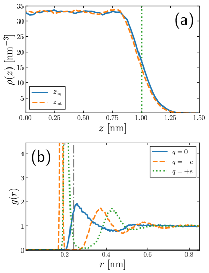
Figure S2: (a) Average solvent density $\rho(z)$, plotted as a function of the coordinate $z$ perpendicular to the liquid-vapor interface, with the solute ($R=0.240$ nm) located in the bulk ($z_{\rm liq}=0$ nm, solid blue line), and at the interface ($z_{\rm int}=1$ nm, dashed orange line). The dotted green line is drawn at $z=z_{\rm int}$. Only half ($z>0$ nm) of the solvent profile is shown. (b) Radial distribution function $g(r)$, plotted as a function of the distance $r$ between the solute’s center and the oxygen atom of a water molecule, with the solute at $z=z_{\rm liq}$ with $q=-e$, $0$, and $+e$. The vertical dot-dashed gray line is drawn at $r=R$.

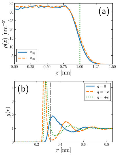
Figure S3: (a) $\rho(z)$ with the solute ($R=0.317$ nm) located in the bulk ($z_{\rm liq}=0$ nm, solid blue line), and at the interface ($z_{\rm int}=1$ nm, dashed orange line). The dotted green line is drawn at $z=z_{\rm int}$. Only half ($z>0$ nm) of the profile is shown. (b) $g(r)$ with the solute at $z=z_{\rm liq}$ with $q=-e$, $0$, and $+e$. The vertical dot-dashed gray line is drawn at $r=R$.

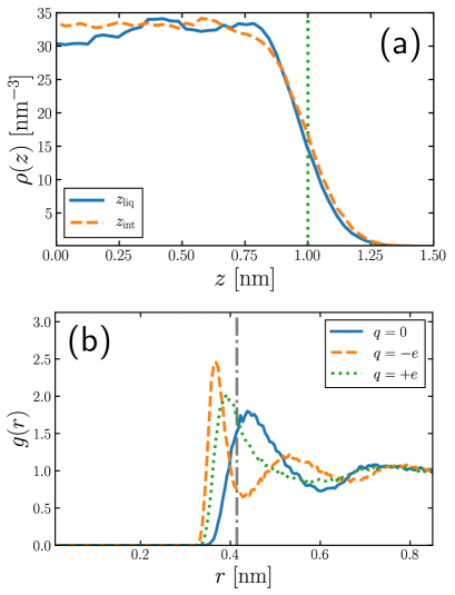
Figure S4: (a) $\rho(z)$ with the solute ($R=0.415$ nm) located in the bulk ($z_{\rm liq}=0$ nm, solid blue line), and at the interface ($z_{\rm int}=1$ nm, dashed orange line). The dotted green line is drawn at $z=z_{\rm int}$. Only half ($z>0$ nm) of the profile is shown. (b) $g(r)$ with the solute at $z=z_{\rm liq}$ with $q=-e$, $0$, and $+e$. The vertical dot-dashed gray line is drawn at $r=R$.

Figure S5: (a) $\rho(z)$ with the solute ($R=0.75$ nm) located in the bulk ($z_{\rm liq}=0$ nm, solid blue line), and at the interface ($z_{\rm int}=1.75$ nm, dashed orange line). The dotted green line is drawn at $z=z_{\rm int}$. Only half ($z>0$ nm) of the profile is shown. (b) $g(r)$ with the solute at $z=z_{\rm liq}$ with $q=-e$, $0$, and $+e$. The vertical dot-dashed gray line is drawn at $r=R$.

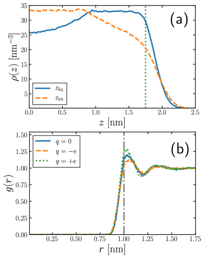
Figure S6: (a) $\rho(z)$ with the solute ($R=1.0$ nm) located in the bulk ($z_{\rm liq}=0$ nm, solid blue line), and at the interface ($z_{\rm int}=1.75$ nm, dashed orange line). The dotted green line is drawn at $z=z_{\rm int}$. Only half ($z>0$ nm) of the profile is shown. (b) $g(r)$ with the solute at $z=z_{\rm liq}$ with $q=-e$, $0$, and $+e$. The vertical dot-dashed gray line is drawn at $r=R$.

S3 Evaluating piecewise linear response

S3.1 Outline

Here we present details of the piecewise linear response (PLR) model discussed in the main article. The PLR model is based on the observation that solvent response to charging a solute is linear for both anions and cations, but differs between the two cases Hummer, Pratt, and García (1996); Lynden-Bell and Rasaiah (1997); Bardhan, Jungwirth, and Makowski (2012). In such a model, the average electrostatic potential due to the solvent at the center of a charged cavity can be written as

$$\langle\phi_{\rm solv}\rangle_{q}=\begin{cases}\phi_{\rm neut}-\beta q\langle(\delta\phi_{\rm solv})^{2}\rangle_{+}\qquad&\text{($q\geq q_{\rm c}$)}\\ \phi_{\rm neut}-\beta q\langle(\delta\phi_{\rm solv})^{2}\rangle_{-}-\beta q_{\rm c}\left[\langle(\delta\phi_{\rm solv})^{2}\rangle_{+}-\langle(\delta\phi_{\rm solv})^{2}\rangle_{-}\right]\qquad&\text{($q<q_{\rm c}$)},\end{cases}$$ (S24)

where $q_{\rm c}$ is the value of the ‘crossover charge’ between the two linear regimes, $\langle(\delta\phi_{\rm solv})^{2}\rangle_{+}$ is the variance of $\phi_{\rm solv}$ for $q\geq q_{\rm c}$, and $\langle(\delta\phi_{\rm solv})^{2}\rangle_{-}$ is the variance of $\phi_{\rm solv}$ for $q<q_{\rm c}$. (As written, it is implicitly assumed that $q_{\rm c}\leq 0$, as suggested by simulations.) Let us define $J=\left[\langle(\delta\phi_{\rm solv})^{2}\rangle_{+}-\langle(\delta\phi_{\rm solv})^{2}\rangle_{-}\right]$. $F_{\rm chg}$ is then,

$$F_{\rm chg}(q)=\begin{cases}q\phi_{\rm neut}-\frac{\beta q^{2}}{2}\langle(\delta\phi_{\rm solv})^{2}\rangle_{+}\qquad&\text{($q\geq q_{\rm c}$)}\\ q\phi_{\rm neut}-\frac{\beta q^{2}}{2}\langle(\delta\phi_{\rm solv})^{2}\rangle_{-}-\beta J\left(qq_{c}-\frac{q_{c}^{2}}{2}\right)\qquad&\text{($q<q_{\rm c}$)},\end{cases}$$ (S25)

and $\psi$ is,

$$\psi(q)=\begin{cases}\phi_{\rm neut}\qquad&\text{($q\leq|q_{\rm c}|$)}\\ \phi_{\rm neut}-\frac{\beta J}{4q}(q-|q_{c}|)^{2}\qquad&\text{($q>|q_{\rm c}|$)}.\end{cases}$$ (S26)

In general, $\phi_{\rm neut}$, $q_{\rm c}$ and $J$ will depend upon solute size, and whether or not the solute is located in bulk or at the interface.

S3.2 Results

Figures S7, S8 and S9 show $\langle\phi_{\rm solv}\rangle_{q}$ vs $q$ for $R=0.240\,{\rm nm},0.317\,{\rm nm}$ and $0.415$ nm, respectively, both for the solute in bulk and at the interface. Note that these results have not been corrected for the finite size of the simulation cell: we will correct $\phi_{\rm neut}$ for finite size effects when computing $\Delta_{\rm ads}\psi^{\rm(PLR)}$, where other finite size effects largely cancel Cox and Geissler (2018). For $R=0.317$ nm and $R=0.415$ nm we can see that PLR is broadly reasonable for the solute in bulk, but some small deviations are seen. These deviations are more pronounced when the solute is at the interface. For $R=0.240$ nm, the above PLR model breaks down at large negative $q$, but it remains reasonable for smaller values of the absolute charge. By fitting straight lines to the anion and cation response, we can obtain values for $q_{\rm c}$, $\langle(\delta\phi_{\rm solv})^{2}\rangle_{+}$ and $\langle(\delta\phi_{\rm solv})^{2}\rangle_{-}$. The results from using these in Eq. S26 to compute $\Delta_{\rm ads}\psi^{\rm(PLR)}$ are presented in Fig. 4b in the main article. Results for $R=0.75$ nm and $R=1$ nm are not shown because, while anion and cation response do still differ, the degree of nonlinearity is much less on an absolute scale than for the smaller solutes. This makes it challenging to reliably obtain $q_{\rm c}$.

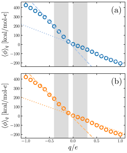
Figure S7: $\langle\phi_{\rm solv}\rangle_{q}$ vs $q$ for $R=0.240$ nm with the solute located (a) in bulk and (b) at the interface. The dashed and dotted lines show linear fits to the left and right shaded regions, respectively.

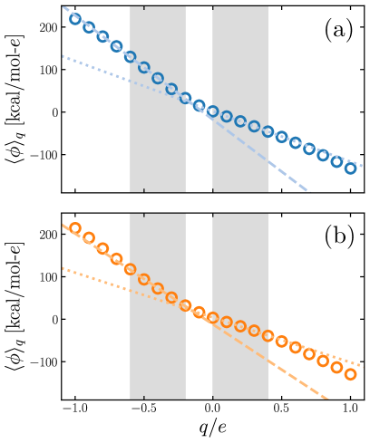
Figure S8: $\langle\phi_{\rm solv}\rangle_{q}$ vs $q$ for $R=0.317$ nm with the solute located (a) in bulk and (b) at the interface. The dashed and dotted lines show linear fits to the left and right shaded regions, respectively.

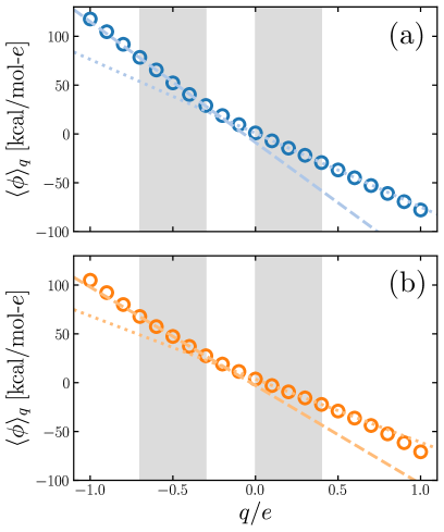
Figure S9: $\langle\phi_{\rm solv}\rangle_{q}$ vs $q$ for $R=0.415$ nm with the solute located (a) in bulk and (b) at the interface. The dashed and dotted lines show linear fits to the left and right shaded regions, respectively.

S4 Constructing $P_{0}(\phi_{\rm solv})$

In order to compute $F_{\rm chg}(q)$ from Eq. 7, we require $P_{0}(\phi_{\rm solv})$, the probability distribution of $\phi_{\rm solv}$. For the range of $q$ of interest, i.e. $-1\leq q/e\leq 1$, sampling $P_{0}$ directly (in the absence of solute charge) would yield grossly insufficient data in the extreme wings of the distribution. Instead, we obtain $P_{0}$ by histogram reweighting using MBAR Shirts et al. (2007). As an illustration, Fig. S10 (a) shows probability distributions $P_{q}(\phi_{\rm solv})$ of $\phi_{\rm solv}$ at the center of the solute ($R=0.240$ nm) with different values of $q$. Using data from simulations across the full range of $q$, we then construct $P_{0}(\phi_{\rm solv})$, as shown in Fig. S10 (b).

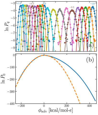
Figure S10: (a) $P_{q}(\phi_{\rm solv})$ for $q/e=-1.0,-0.9,\ldots,0.0,\ldots,0.9,1.0$ with $R=0.240$ nm. Solid lines indicate normalized Gaussian distributions and are included as a guide to the eye. (b) $P_{0}(\phi_{\rm solv})$ reconstructed from the set of $P_{q}$ using MBAR Shirts et al. (2007) (solid line). The dashed line indicates a normalized Gaussian distribution with mean and variance obtained from the simulation at $q/e=0$. Note that finite size corrections have not been applied to these plots.