Two-sample hypothesis testing for latent distance graphs with unknown link functions

Abstract

We propose a valid and consistent test for the hypothesis that two latent distance random graphs on the same vertex set have the same generating latent positions, up to some unidentifiable similarity transformations. Our test statistic is based on first estimating the edge probabilities matrices by truncating the singular value decompositions of the averaged adjacency matrices in each population and then computing a Spearman rank correlation coefficient between these estimates. Experimental results on simulated data indicate that the test procedure has power even when there is only one sample from each population, provided that the number of vertices is not too small. Application on a dataset of neural connectome graphs showed that we can distinguish between scans from different age groups while application on a dataset of epileptogenic recordings showed that we can discriminate between seizure and non-seizure events.

Keywords: Graph inference; Latent distance graphs model; Two-sample hypothesis testing.

1 Introduction

In recent years, the increasing popularity of network data in diverse fields has spurred significant developments in many theoretical and applied research related to random graph models and their statistical inference [Erdős and Rényi, 1960, Hoff et al., 2002, Handcock et al., 2007, Wasserman and Pattison, 1996, Holland et al., 1983, Airoldi et al., 2008, Karrer and Newman, 2011]. A significant amount of literature on statistical inference for random graphs has focused on estimation [Chatterjee, 2015, Xu, 2018, Olhede and Wolfe, 2014] and community detection; see [Abbe, 2017] and the references therein for a survey of recent progresses on community detection.

In contrasts, the problem of graph comparisons or two-sample hypothesis testing on random graphs has not been as well studied in statistics. Graph comparisons are widely used in neuroscience, with two prominent approaches. One approach advocates comparing the edges directly as a collection of paired $t$-tests [Zalesky et al., 2010] while the other proposes to compare graph-theoretic measures such as the clustering coefficient, path length, and their ratio [Rubinov and Sporns, 2010, He et al., 2008, Humphries and Gurney, 2008]. These two approaches, while useful, have their own disadvantages. In particular, the pairwise comparison of edges views a network on $n$ vertices as a collection of $n(n-1)/2$ edges and ignores any underlying network structure or topology. The use of graph-theoretic measures, meanwhile, implicitly assumes that a graph can be reasonably summarized by a few graph invariants. It is, however, not a priori clear which invariants are appropriate and oftentimes a graph invariant is chosen due to its computational cost, e.g., number of triangles versus general cliques. Finally, neither of these approaches consider the statistical implications in term of validity and consistency of the test procedures.

In statistics literature, several methods have been investigated recently. [Ginestet et al., 2017] derived a central limit theorem for the sample Fréchet mean of combinatorial graph Laplacians and built a Wald-type two-sample test statistic. [Ghoshdastidar et al., 2020] proposed to compare the underlying graph-generating distributions with a test statistic based on differences of the estimated edge-probability matrices with respect to the spectral or Frobenius norms. [Ghoshdastidar and von Luxburg, 2018] further developed a test statistic via extreme eigenvalues of a scaled and centralized matrix as motivated by the Tracy-Widom law. The aforementioned literature generally does not assume any specific generative model for the observed graphs. For example, [Ginestet et al., 2017] only assumes that the vertices are aligned while [Ghoshdastidar et al., 2020] and [Ghoshdastidar and von Luxburg, 2018] only require conditional independence of edges. There is then an inherent tradeoff between generality of the generative model and specificity of the theoretical results; indeed, for these models, a graph on $n$ vertices could require $n(n-1)/2$ parameters for the pairwise edge probabilities. To address the potential need for estimating these parameters, [Ginestet et al., 2017] assume that the number of graphs is reasonably large compared to the number of vertices, while the necessary conditions for consistency of the test statistics in [Ghoshdastidar et al., 2020] and [Ghoshdastidar and von Luxburg, 2018] are quite complex.

Various popular generative graph models such as the stochastic block model, latent space model and their variants, have also been actively studied in the context of two-sample testing problems. Stochastic block model graphs, first introduced by [Holland et al., 1983], assume that vertices are partitioned into several unobserved blocks and the probability of connection is a function of block membership. Under this model, [Li and Li, 2018] studied the problem of testing the differences of block memberships and constructed test statistic via singular subspace distance. The notion of hidden communities in stochastic blockmodel graphs can be generalized to yield latent space model graphs or graphons [Hoff et al., 2002, Bollobas et al., 2007, Lovász, 2012]. In the latent space model each vertex $v_{i}$ is associated with a latent position $x_{i}\in\mathbb{R}^{d}$ and, conditioned on the latent positions of these vertices, the edges are independent Bernoulli random variables with mean $p_{ij}=f(x_{i},x_{j})$ where $f$ is a symmetric link function. A special case of a latent space model is the notion of a generalized random dot product graph [Young and Scheinerman, 2007, Rubin-Delanchy et al., 2017] wherein $f(x_{i},x_{j})=\langle x_{i},x_{j}\rangle$ for some inner product or bilinear form $\langle\cdot,\cdot\rangle$. Random dot product graphs include, as a special case, stochastic blockmodel graphs and its degree-corrected and mixed-membership variants, and furthermore, any latent position graphs can be represented as a random dot product graph with a fixed dimension $d$ or be approximated arbitrarily well by a random dot product graph with growing $d$. For the random dot product graphs, [Tang et al., 2017a] considered the two-sample problem of determining whether or not two graphs on the same vertex set have the same generating latent positions or have generating latent positions that are scaled or diagonal transformations of one another; [Tang et al., 2017b] studied a related problem wherein the graphs can have different vertex sets with possibly differing numbers of vertices. Another special case of the latent space model specifies that $f$ is the logit link function and for this choice of $f$, [Durante et al., 2018] developed a Bayesian procedure for testing group differences in the network structure that also relies on a low-rank representation of the latent positions together with edge-specific latent covariates.

The appeal, and consequently power and utility, of the latent space formulation for two-sample testing stems from the fact that a $n$ vertices graph can be parameterized by the $n\times d$ matrix of latent positions $\{x_{i}\}$; this is, when $n\gg d$, a considerable reduction in the number of parameters compared to the $n(n-1)/2$ edge probabilities. This reduction, however, is possible only if the $\{x_{i}\}$ can be estimated accurately, and this is generally done by assuming that $f$ is known; e.g., $f$ is a bilinear form [Tang et al., 2017a, Tang et al., 2017b] or the logistic function [Durante et al., 2018].

We consider in this paper another two-sample testing problem for latent position graphs, but, in contrasts to existing works we neither assume that the link function $f$ is known nor that it need to be the same between the two-samples. More specifically, we consider the class of latent distance random graphs wherein we assume that $f(x_{i},x_{j})=h(\|x_{i}-x_{j}\|)$ for some unknown non-increasing function $h$ that could differ between the two samples. It is not a priori clear that the latent positions are even identifiable; we show subsequently that the latent positions are identifiable up to a similarity transformation.

The problem is of significant theoretical and practical interest because of the following reasons. The first is that many of the currently studied two-sample testing problems have test statistics that are constructed using the difference of adjacency matrices or the estimated edge probability matrices. Since we assume the link function is unknown and possibly different, this commonly used method is no longer valid. As we will clarify later, even when we know that the link functions are of the same form, they may still depend on unknown parameters that are different between the two samples, and thus we have different edge-probability matrices which cannot be compared directly. The second reason is that, due to the non-identifiability of latent positions, our test procedures allow for more flexible comparisons than just whether or not the two latent positions are exactly the same, i.e., our tests are for equality up to general similarity transformation which includes any transformation that preserves the ordering of pairwise distances.

Our test procedure, even after accounting for all this complex source of non-identifiability, is quite simple. We estimate the edge probabilities matrices by truncating the singular value decomposition of the averaged adjacency matrices in each population and then compute our test statistic as the Spearman rank correlation between these estimates. Significance values are obtained either via a permutation test when the number of samples from each population is moderate, or via a bootstrapping scheme in the case when there are only one or two samples in each population.

2 Methodology

We first recall the definition of latent distance random graphs [Hoff et al., 2002].

Definition 1 (Latent Distance Random Graphs).

Let $h$ be a monotone decreasing function from $\mathbb{R}$ to $[0,1]$ and assume $h(0)=1$ for identifiability. Let $n,d\geq 1$ be given and let $X=[x_{1}\mid\dots\mid x_{n}]^{\top}$ be a $n\times d$ matrix with rows $x_{i}\in\mathbb{R}^{d}$. A $n\times n$ adjacency matrix $A$ is said to be an instance of a latent distance random graph with latent position $X$ and sparsity parameter $\rho\in(0,1]$ if $A$ is a symmetric, hollow matrix whose upper triangular entries $a_{ij},i<j$ are conditionally independent Bernoulli random variables with $\mathrm{pr}(a_{ij}=1)=\rho h(\|x_{i}-x_{j}\|)$, i.e., the likelihood of $A$ given $X$ is

$$\mathrm{pr}(A|X)=\prod_{i<j}\left\{\rho h(\|{x}_{i}-{x}_{j}\|)\right\}^{a_{ij}}\left\{1-\rho h(\|{x}_{i}-{x}_{j}\|)\right\}^{1-a_{ij}}.$$

The graphs we study are undirected, unweighted and loop-free. Given two adjacency matrices $A$ and $B$ for a pair of random latent distance graphs on the same set of vertices, we will propose a valid, consistent test to determine whether the two generating latent positions are equal up to similarity transformation, e.g., scaling and orthogonal transformation.

Generally speaking, the link functions are unknown. Even when the specific form of the link functions are known, there could still be unknown parameters. For example, the original latent space model of [Hoff et al., 2002] uses the logistic function, i.e.,

$$h(\|{x}_{i}-{x}_{j}\|)=\frac{\exp(\alpha-\beta\|{x}_{i}-{x}_{j}\|)}{1+\exp(\alpha-\beta\|{x}_{i}-{x}_{j}\|)},$$

where $\alpha\in\mathbb{R}$ and $\beta>0$. Other alternatives were discussed in [Raftery, 2017]. [Gollini and Murphy, 2016] replaced the Euclidean distance by the squared distance to allow higher edge-probability for close points. [Rastelli et al., 2016] replaced the logistic function by a Gaussian kernel

$$h(\|{x}_{i}-{x}_{j}\|)=\gamma\exp\left(-\frac{\|{x}_{i}-{x}_{j}\|^{2}}{2\phi}\right),$$

where $\gamma\in[0,1]$ and $\phi>0$. Even if the link functions of networks to be compared are known and in the same form, it is still reasonable for them to have different parameters, such as $\alpha,\beta$ in the logistic function and $\gamma,\phi$ in the Gaussian function. Furthermore, even when the link functions are the same with exactly identical parameters, if the latent positions are similar up to an unknown similarity transformation then the edge-probability matrices are not equal and cannot be compared directly. We are thus motivated to consider the following two-sample hypothesis testing problem.

Let $X,Y\in\mathbb{R}^{n\times d}$. We define the edge-probability matrices $P=(p_{ij})\in\mathbb{R}^{n\times n}$ where $p_{ij}=h(\|{x}_{i}-{x}_{j}\|)$ and $Q=(q_{ij})\in\mathbb{R}^{n\times n}$ where $q_{ij}=g(\|{y}_{i}-{y}_{j}\|)$. The link functions $h$ and $g$ are unknown and possibly different. We shall assume, for identifiability, that $h(0)=g(0)=1$. Given $A_{1},...,A_{m}$ and $B_{1},...,B_{m}$ generated from latent distance random graphs with latent positions $X$ and $Y$ respectively, where $m\geq 1$, the two-sample testing problem is defined formally as

$$H_{0}:X=sYW+1t^{\top}\text{ for some $s\in\mathbb{R}$, orthogonal $W\in\mathbb{R}^{d\times d}$, ${t}\in\mathbb{R}^{d}$ against}$$

$$H_{a}:X\neq sYW+1t^{\top}\text{ for any $s\in\mathbb{R}$, orthogonal $W\in\mathbb{R}^{d\times d}$, ${t}\in\mathbb{R}^{d}$}.$$

The above null hypothesis captures the notion that two latent positions are the same up to similarity transformations.

Our test procedure starts by estimating the edge-probability matrices using a singular value thresholding procedure. More specifically, we compute $\bar{A}=m^{-1}\sum_{i}A_{i}$ and let $\hat{P}$ be the best rank-$K$ approximation of $\bar{A}$ with respect to the Frobenius norm, i.e., $\hat{P}$ is obtained by computing the singular value decomposition of $\bar{A}$ and keeping only the $K$ largest singular values and corresponding singular vectors. The estimate $\hat{Q}$ of $Q$ is constructed similarly. Singular value thresholding procedures have been actively studied in [Chatterjee, 2015] and [Xu, 2018]. As discussed in [Xu, 2018], the choice of dimension $K$ can be determined by a threshold $\tau=c_{0}(n\rho)^{1/2}$ where $c_{0}$ is a universal constant strictly larger than $4$ in the case of $n\rho\gg\log(n)$ and strictly larger than $2$ in the case of $n\rho\gg\log^{4}(n)$. For our simulation and real data analysis, we frequently set $K$ to a fixed value or choose $K$ using the dimension selection procedure of [Zhu and Ghodsi, 2006].

Since the link function is assumed to be monotone in latent distance random graphs, under the null hypothesis, the ordering of the entries in the two edge-probability matrices should be the same, i.e., $p_{ij}\leq p_{k\ell}$ if and only if $q_{ij}\leq q_{k\ell}$. Thus, several rank-based or order-based methods can be used to construct similar test statistic, including Kendall’s $\tau$ coefficient, Spearman’s rank correlation coefficient, non-metric multidimensional scaling and isotonic regression. There are, however, important computational or theoretical challenges for some of these methods. In particular, Kendall’s $\tau$ is computationally intensive with $O(n^{4})$ time complexity where $n$ is the number of vertices. An approximation for Kendall’s $\tau$ with $O(n^{2}\log n)$ complexity has been developed but its impact on the theoretical properties of the resulting test statistic is unknown. Non-metric multidimensional scaling is also computationally intensive as it is generally formulated as a non-convex problem with multiple local minima and thus one is not guaranteed to find the global minimum. Using isotonic regression, we can consider $p_{ij}=f(q_{ij})$ and test whether the function $f$ is monotone, but the corresponding theory in the case where the predictor variable is noisy has not been well-studied.

We thus propose a test statistic defined using Spearman’s rank correlation coefficient, which is computationally efficient with $O(n^{2})$ complexity. That is,

$$T_{n}(\hat{P},\hat{Q}) =\frac{\mathrm{cov}\{R(\hat{P}),R(\hat{Q})\}}{\hat{\sigma}\{R(\hat{P})\}\hat{\sigma}\{R(\hat{Q})\}},$$ (2.1)

where $R(\hat{P})\in\mathbb{R}^{n\times n}$ and $R(\hat{Q})\in\mathbb{R}^{n\times n}$ are symmetric matrices whose entries are the ranks of the corresponding entries in $\hat{P}$ and $\hat{Q}$, $\mathrm{cov}\{R(\hat{P}),R(\hat{Q})\}$ is the sample covariance of these ranks, and $\hat{\sigma}\{R(\hat{P})\}$ and $\hat{\sigma}\{R(\hat{Q})\}$ are the standard deviations. Given the significance level $\alpha\in(0,1)$, the rejection region $\mathcal{R}$ for the test statistic $T_{n}$ is $\mathcal{R}=\left\{t|\text{ $p$-value}(t)<\alpha\right\}$, where $\text{$p$-value}(t)$ can be determined either via a permutation test or via a bootstrapping procedure as described in Algorithm 1. When the number of samples from each population is moderately large then both methods should perform well. If the number of samples is small, or even in the case when there is only a single network observation for each population, then the bootstrap could be more robust.

Input: Two adjacency matrices $A,B\in\mathbb{R}^{n\times n}$. Number of bootstrap replications $N$.

1. Apply universal singular value thresholding on $A$ and $B$ to get $\hat{P}$ and $\hat{Q}$.

2. Calculate test statistic as $t^{*}:=T_{n}(\hat{P},\hat{Q})$.

For $k=1,...,N$, repeat steps 3, 4 and 5:

1. Generate $A_{1}^{(k)}=\left(a_{1,ij}^{(k)}\right)_{n\times n}$, $A_{2}^{(k)}=\left(a_{2,ij}^{(k)}\right)_{n\times n}$, $B_{1}^{(k)}=\left(b_{1,ij}^{(k)}\right)_{n\times n}$ and $B_{2}^{(k)}=\left(b_{2,ij}^{(k)}\right)_{n\times n}$ as

   $$a_{1,ij}^{(k)}\overset{i.i.d}{\sim}\text{Bernoulli}(\hat{p}_{ij}),\quad a_{2,ij}^{(k)}\overset{i.i.d}{\sim}\text{Bernoulli}(\hat{p}_{ij}),$$

   $$b_{1,ij}^{(k)}\overset{i.i.d}{\sim}\text{Bernoulli}(\hat{q}_{ij}),\quad b_{2,ij}^{(k)}\overset{i.i.d}{\sim}\text{Bernoulli}(\hat{q}_{ij}).$$

2. Apply universal singular value thresholding on the bootstrapped adjacency matrices to get $\hat{P}_{1}^{(k)}$, $\hat{P}_{2}^{(k)}$, $\hat{Q}_{1}^{(k)}$ and $\hat{Q}_{2}^{(k)}$.

3. Calculate test statistic as $t_{P}^{(k)}:=T_{n}\left(\hat{P}_{1}^{(k)},\hat{P}_{2}^{(k)}\right)$ and $t_{Q}^{(k)}:=T_{n}\left(\hat{Q}_{1}^{(k)},\hat{Q}_{2}^{(k)}\right)$

4. Calculate the $p$-value as

   $$\text{$p$-value}=\min\left[\max\left\{\frac{1}{N}\sum_{k=1}^{N}I\left(t^{*}<t_{P}^{(k)}\right),\frac{1}{N}\sum_{k=1}^{N}I\left(t^{*}<t_{Q}^{(k)}\right)\right\},1\right].$$

Output: $p$-value of the proposed testing procedure.

Algorithm 1 Bootstrap

3 Main Results

We now establish the main theoretical properties of the proposed test procedure as the number of vertices $n$ increases. We will assume that the number of graphs $m$ in each sample, is bounded; thus, for ease of exposition, we set $m=1$ throughout. The case when $m\rightarrow\infty$ with increasing $n$ is considerably simpler and is thus ignored.

We start by introducing several mild assumptions on the link functions $h$ and $g$ and the latent positions $\{x_{i}\}_{i=1}^{n}$ and $\{y_{i}\}_{i=1}^{n}$.

Assumption 1.

As $n\to\infty$, for any $\epsilon>0$, there exists $\delta>0$ such that $[0,1)$ can be partitioned into the union of intervals of the form $[(k-1)\delta,k\delta)$ for $k=1,...,\lceil 1/\delta\rceil$, such that, for any $k$, one of the following two conditions holds almost surely:

1. Either the number of $ij$ pairs with $i<j$ and $p_{ij}\in[(k-1)\delta,k\delta)$ is at most $n(n-1)\epsilon/2$.

2. Or if the number of $ij$ pairs with $i<j$ and $p_{ij}\in[(k-1)\delta,k\delta)$ exceeds $n(n-1)\epsilon/2$, then they are all equal for $p_{ij}\in[(k-1)\delta,k\delta)$.

Assumption 2.

Define

$$\hat{\sigma}\{R(P)\}=\Bigl{[}\tbinom{n}{2}^{-1}\sum_{i<j}\Bigl{\{}R(p_{ij})-\tbinom{n}{2}^{-1}\sum_{i<j}R(p_{ij})\Bigr{\}}^{2}\Bigr{]}^{1/2}$$

as the sample variance for the ranks of the entries in $P$. Define $\hat{\sigma}\{R(Q)\}$ similarly. Then as $n\rightarrow\infty$, $\hat{\sigma}\{R(P)\}=\Omega(n^{2})$ and $\hat{\sigma}\{R(Q)\}=\Omega(n^{2})$ almost surely.

Assumption 3.

The link functions $h$ and $g$ are fixed with $n$ and both are infinitely differentiable. The latent positions $x_{i}\in U\subset\mathbb{R}^{d}$and $y_{i}\in V\subset\mathbb{R}^{d}$ for some fixed compact sets $U$ and $V$ that do not depend on $n$.

Assumption 4.

There exists a constant $C$ not depending on $n$ such that, as $n$ increases, the sparsity parameter $\rho\in(0,1]$ satisfies $n\rho\geq C\log n$.

Remark 1.

We now explain the rationale behind the above assumptions.

1. Assumption 1 prevents the setting where a large number of latent positions concentrate around a single point $x_{0}$ with increasing $n$ but that these points are not equal to $x_{0}$. If this happens then the values of the $p_{ij}$ for this collection of points would be almost identical but their ranks are substantially different. For example, suppose there are $cn$ points around a small neighbourhood of $x_{0}$. Then the $p_{ij}$ for the $cn(cn-1)/2$ pairs in this neighbourhood will all be approximately $h(0)$. The rank of the smallest and the largest of these $p_{ij}$ could, however, differ by $cn(cn-1)/2$. Assumption $1$ arises purely because we do not assume anything about a generative model for the latent positions $\{x_{i}\}$. Indeed, if the latent positions $x_{i}$ are independent and identically distributed samples from some distribution $F$, then for any point $x_{0}$, either $F$ has an atom at $x_{0}$ which will then force $p_{ij}=c$ for some constant $c$ whenever $x_{i}=x_{j}=x_{0}$. Otherwise, if $F$ is non-atomic at $x_{0}$ then the proportion of points $x_{i}$ with $\|x_{i}-x_{0}\|\leq\delta$ will converge to $0$ as $\delta\rightarrow 0$.

2. Assumption 2 complements Assumption 1 and prevents the ranks of the entries of $P$ and $Q$ from being degenerate. Suppose, for example, that there are $n-o(n)$ points located at a certain position ${x}_{0}$. In this case, $\hat{\sigma}\{R(P)\}=o(n^{2})$. The problem of testing whether $X$ is equal to $Y$ up to a similarity transformation can thus be reduced to consider only the subgraphs induced by these $o(n)$ points. We can then apply the test procedure in this paper, assuming that these induced subgraphs can be found efficiently. The problem of identifying these subgraphs is, however, outside the scope of our current investigation.

3. Assumption 3 restricts the smoothness of the link functions. This is done entirely for ease of exposition. The assumption can easily be relaxed as it only affects the accuracy of the universal singular value thresholding procedure used in estimating edge-probability, which in turn affects the convergence rate of the test statistic. More specifically, suppose the link function $h$ belongs to a Hölder class or Sobolev class with index $\omega$. Then Theorem 1 of [Xu, 2018] implies that

   $$\frac{1}{n^{2}}\|\hat{P}-P\|_{F}^{2}=O_{p}\left((n\rho)^{-\frac{2\omega}{2\omega+d}}\right).$$

   The convergence rate of our test statistic will then depends on $\omega$ and is thus slower than the convergence rate for infinitely differentiable link functions as given in Corollary 1.

4. Assumption 4 is identical to that used in [Xu, 2018]. We restrict the sparsity of the observed graphs in order to guarantee that the singular value thresholding estimates $\hat{P}$ and $\hat{Q}$ are accurate estimates of $P$ and $Q$.

With the above assumptions in place, we now show that the test statistic $T_{n}$ constructed using appropriately discretized versions of the estimated edge probabilities matrices $\hat{P}$ and $\hat{Q}$ is, asymptotically, the same as that constructed using the true $P$ and $Q$. The need for discretizing the entries of $\hat{P}$ and $\hat{Q}$ is due mainly to the fact that the estimates $\{\hat{p}_{ij}\}$ and $\{\hat{q}_{ij}\}$ are inherently noisy. Suppose for example that $p_{ij}=0.1$ for all $ij$ pairs. Then $R(p_{ij})\equiv\{n(n-1)/2+1\}/2$, the average of the ranks in $\{1,...,n(n-1)/2\}$. However, because of the estimation error, the $\hat{p}_{ij}$ might contain numerous distinct values like $\{0.101,0.102,...\}$ and thus $\sum_{i<j}\{R(p_{ij})-R(\hat{p}_{ij})\}^{2}$ can be quite large even though the estimates $\hat{p}_{ij}$ are all approximately equal to the true $p_{ij}$. We are thus motivated to consider a more robust estimator obtained by discretizing the $\{\hat{p}_{ij}\}$, i.e., let $\eta>0$ and define the $\eta$-discretization of $\hat{p}_{ij}$ as

$$\tilde{p}_{ij}=\left\lceil\frac{\hat{p}_{ij}}{\eta}\right\rceil\times\eta.$$

Recall the above example. By letting $\eta=0.01$, we have $\tilde{p}_{ij}=0.1$ provided that $\mid\hat{p}_{ij}-0.1\mid\leq 0.01$ and hence the ranks of these $\tilde{p}_{ij}$ are the same. We emphasize that while this discretization step simplifies the subsequent theory considerably, it is not essential in real data analysis as we can always choose $\eta$ sufficiently small so that $\tilde{p}_{ij}$ is arbitrarily close to $\hat{p}_{ij}$.

Theorem 3.1.

Assume Assumptions 1–4 hold. Then for sufficiently large $n$,

$$T_{n}(\tilde{P},\tilde{Q})-T_{n}(P,Q)=o_{p}(1).$$

Here $\tilde{P}$ and $\tilde{Q}$ are the $\eta$-discretization of $\hat{P}$ and $\hat{Q}$ with $(\eta^{2}\rho)^{-1}=o(n)$ as $n\rightarrow\infty$.

Theorem 3.1 indicates that $T_{n}(\tilde{P},\tilde{Q})-T_{n}(P,Q)$ converges to $0$ as $n\rightarrow\infty$. There are, however, instances in which we are interested in the rate of convergence of $T_{n}(\tilde{P},\tilde{Q})-T_{n}(P,Q)$ to $0$. We derive the rate of convergence under the following more restrictive version of Assumption 1.

Assumption 5.

There exists a constant $c>0$ independent of $\delta$ such that for $k=1,\dots,\lceil 1/\delta\rceil$,

$$\mid\{(i,j):p_{ij}\in[(k-1)\delta,k\delta]\}\mid\leq c\cdot\delta\tbinom{n}{2}.$$

Corollary 1.

Under the conditions in Theorem 3.1 and Assumption 5, we have

$$T_{n}(\tilde{P},\tilde{Q})-T_{n}(P,Q)=O_{p}(\epsilon^{1/2}),$$

where $(\epsilon^{2}\rho)^{-1}=o(n)$.

Assumption 5 allows us to set $\eta=\epsilon=c\delta$ in the proof of Theorem 3.1, thereby yielding the convergence rate of $O_{p}(\epsilon^{1/2})$ in Corollary 1. If the conditions in Assumption 5 are not satisfied then there is, a priori, no explicit relationship between $\eta$ and $\epsilon$ other than that $\epsilon\to 0$ as $\eta\to 0$.

If the null hypothesis is true then $T_{n}(P,Q)=1$ and hence, from Theorem 3.1, we have $T_{n}(\tilde{P},\tilde{Q})\rightarrow 1$ almost surely as $n\rightarrow\infty$. A natural question then is whether or not $T_{n}(\tilde{P},\tilde{Q})\rightarrow 1$ also indicates that the matrix of latent positions $X$ is close, up to some similarity transformation, to the matrix of latent positions $Y$ ? To address this question we shall assume that the sequences of latent positions $\{x_{i}\}_{i=1}^{n}$ and $\{y_{i}\}_{i=1}^{n}$ satisfy the following denseness conditions as $n\rightarrow\infty$.

Assumption 6.

Let $U\subset\mathbb{R}^{d}$ and $V\subset\mathbb{R}^{d}$ be non-empty, bounded and connected sets. Let $\Omega_{n}=\{{x}_{1},...,{x}_{n}\}\subset U$ and $\Xi_{n}=\{y_{1},y_{2},\dots,y_{n}\}\subset V$. Then $\lim_{n\rightarrow\infty}\Omega_{n}$ and $\lim_{n\rightarrow\infty}\Xi_{n}$ are dense in $U$ and $V$, respectively. Furthermore, for any $\epsilon>0$ there exist $\delta_{U}=\delta_{U}(\epsilon)>0$ and $\delta_{V}=\delta_{V}(\epsilon)>0$ depending on $\epsilon$ such that

$$n^{-1}\liminf|B(x,\epsilon)\cap\Omega_{n}|\geq\delta_{U},\qquad\text{for all $x\in U$},$$

$$n^{-1}\liminf|B(y,\epsilon)\cap\Xi_{n}|\geq\delta_{V},\qquad\text{for all $y\in V$}.$$

Here $B(x,\epsilon)$ denote the ball of radius $\epsilon$ centered at $x$.

Assumption 6 is a regularity condition for the minimum number of latent positions $\{x_{i}\}$ and $\{y_{i}\}$ in any arbitrarily small, but non-vanishing subset of $U$ and $V$. In particular, Assumption 6 prevents the setting where, as $n\rightarrow\infty$, the sequence of latent positions $\{x_{i}\}_{i=1}^{n}$ is dense in $U$, but that, for any sufficiently large $n$, all except $o(n)$ of these $\{x_{i}\}$ are concentrated at some fixed $K$ points $\nu_{1},\dots\nu_{K}\in U$, i.e., the denseness of the $\{x_{i}\}_{i=1}^{n}$ is due to a vanishing fraction of the points. While the removal of these $o(n)$ points from both $\{x_{i}\}$ and $\{y_{i}\}$ does not change the convergence $T_{n}(P,Q)$ to $1$, it will lead to very different geometry for the remaining latent positions. In summary, as we only require $T_{n}(P,Q)\rightarrow 1$, Assumption 6 guarantees that the removal of any $o(n)$ points from the $\{x_{i}\}$ and $\{y_{i}\}$ does not substantially change the geometry of the remaining points, especially since the removal of any $o(n)$ points does not change the convergence of $T_{n}(P,Q)$.

The following result showed that if $X$ and $Y$ satisfy the conditions in Assumption 6 and $T_{n}(P,Q)\rightarrow 1$ as $n\rightarrow\infty$ then the Frobenius norm distance between $X$ and some similarity transformation of $Y$ is of order $o(n^{1/2})$. Since there are $n$ rows in $X$ and $Y$, this indicates that for any arbitrary but fixed $\epsilon>0$, the number of rows $i$ such that $\|X_{i}-sWY_{i}-t\|\geq\epsilon$ is of order $o(n)$ as $n$ increases. That is to say, almost all rows of $X$ are arbitrarily close to the corresponding rows of some similarity transformation of $Y$.

Theorem 3.2.

Suppose that, as $n\rightarrow\infty$, the latent positions $X$ and $Y$ satisfy Assumption $1$ through $4$ together with Assumption $6$. If $T_{n}(P,Q)\to 1$ as $n\to\infty$ then there exists $s\in\mathbb{R}$, orthogonal matrix $W\in\mathbb{R}^{d\times d}$ and $t\in\mathbb{R}^{d}$ such that

$$\|X-sYW-1t^{\top}\|_{F}=o(n^{1/2}).$$

The detailed proofs of Theorem 3.1 and Theorem 3.2 are given in the supplementary materials.

We finally discuss the consistency of our test procedure. Since, as $n$ increases, the dimension of our latent positions and the associated edge probabilities matrices also increases, we shall define consistency of our test procedure in the context of a sequence of hypothesis tests.

Definition 2 (Consistency).

Let $(X_{n},Y_{n})_{n\in\mathbb{N}}$ be a given sequence of latent positions, where $X_{n}$ and $Y_{n}$ are both in $\mathbb{R}^{n\times d}$. A test statistic $T_{n}$ and associated rejection region $\mathcal{R}$ to test the hypothesis

$$\begin{split}&H_{0}:X=sYW+1t^{\top}\text{ for some $s\in\mathbb{R}$, orthogonal $W\in\mathbb{R}^{d\times d}$, ${t}\in\mathbb{R}^{d}$ against}\\ &H_{a}:X\neq sYW+1t^{\top}\text{ for any $s\in\mathbb{R}$, orthogonal $W\in\mathbb{R}^{d\times d}$, ${t}\in\mathbb{R}^{d}$}.\end{split}$$

is a consistent, asymptotically level $\alpha$ test if for any $\epsilon>0$, there exists $n_{0}=n_{0}(\epsilon)$ such that:

1. If $n>n_{0}$ and $H_{a}^{n}$ is true, then $\mathrm{pr}(T_{n}\in\mathcal{R})>1-\epsilon$.

2. If $n>n_{0}$ and $H_{0}^{n}$ is true, then $\mathrm{pr}(T_{n}\in\mathcal{R})\leq\alpha-\epsilon$.

Theorem 3.3.

Let $\{X_{n}\}_{n\geq 1}$ and $\{Y_{n}\}_{n\geq 1}$ be two sequences of matrices of latent positions for the latent position graphs with link functions $g$ and $h$, respectively. Suppose that, as $n\rightarrow\infty$, these latent positions and associated link functions satisfy Assumptions $1$ through $4$ together with Assumption $6$. For each fixed $n$, consider the hypothesis test in Definition 2 for the $X_{n}$ and $Y_{n}$. Define the test statistic $T_{n}(\tilde{P},\tilde{Q})$ as in Eq.(2.1). Let $\alpha\in(0,1)$ be given. If the rejection region is $\mathcal{R}=\{t\in\mathbb{R}:t<C\}$ for some constant $C\leq 1$, then there exists an $n_{0}=n_{0}(\alpha,\epsilon)\in\mathbb{N}$ such that for all $n\geq n_{0}$, the test procedure with $T_{n}$ and the rejection region $\mathcal{R}$ is an at most level $\alpha$ test, that is, if the null hypothesis $H_{0}$ is true, then $\mathrm{pr}(T_{n}\in\mathcal{R})\leq\alpha-\epsilon$. Denote by

$$d_{n}=\min_{s,W,t}\|X_{n}-sY_{n}W-1t^{\top}\|_{F}$$

the minimum Frobenius norm distance, up to some similarity transformation, between $X_{n}$ and $Y_{n}$. Then the test procedure is consistent in the sense of Definition 2 over this sequence of latent positions if, as $n\rightarrow\infty$, $\liminf n^{-1/2}d_{n}I\{d_{n}>0\}>0$ where $I(\cdot)$ is the indicator function.

Remark 2.

In Theorem 3.3, $\alpha$ need not depend on $C$ since we have not derived a non-degenerate limiting distribution for our test statistic. Theorem 3.3 indicates that, for sufficiently large $n$, our test procedure has power arbitrarily close to $1$ whenever the minimum Frobenius norm distance between $X_{n}$ and any similarity transformation of $Y_{n}$ is of order $\Omega(n^{1/2})$. Thus, roughly speaking, the test procedure has power converging to $1$ if there does not exists a similarity transformation mapping the rows of $X_{n}$ to that of $Y_{n}$; see the discussion prior to the statement of Theorem 3.2.

4 Simulations

4.1 General Procedure

We first summarize the setup and general procedure used for generating the empirical distributions of our test statistic.

1. For $i=1,...,n$ and $j=1,2$, generate $x_{ij}\overset{iid}{\sim}N(0,1)$ and form $X=(x_{ij})\in\mathbb{R}^{n\times 2}$.

2. We set different $Y$ for null and alternative hypotheses:

   • Under $H_{0}$: Set $Y=(1+\epsilon)X$.

   • Under $H_{a}$: Set $Y=X+Z$ where $Z=(z_{ij})\in\mathbb{R}^{n\times 2}$ and $z_{ij}\overset{iid}{\sim}N(0,\epsilon)$ independent from $x_{ij}$.

3. The edge-probability matrices based on $X$ and $Y$ are respectively defined as $P=(p_{ij})\in\mathbb{R}^{n\times n}$ and $Q=(q_{ij})\in\mathbb{R}^{n\times n}$, where

   $$p_{ij}=h({x}_{i},{x}_{j}) =\exp(-\|{x}_{i}-{x}_{j}\|^{2}),\qquad q_{ij}=g({y}_{i},{y}_{j}) =\exp(-\|{y}_{i}-{y}_{j}\|^{2}/4).$$

4. Generate the corresponding adjacency matrices $A$ and $B$ as $A_{ii}=B_{ii}=0$ for $i=1,...,n$ and $A_{ij}=\text{Bernoulli}(\rho p_{ij})$, $B_{ij}=\text{Bernoulli}(\rho q_{ij})$ for $i,j=1,...,n$ and $i\neq j$.

5. Apply universal singular value thresholding on $A$ and $B$ to get the estimates of $P$ and $Q$ as $\hat{P}$ and $\hat{Q}$.

6. Calculate the test statistic $T_{n}(\hat{P},\hat{Q})$.

7. Repeat (d)-(f) 100 times or use other resampling techniques to get the empirical distribution of $T_{n}(\hat{P},\hat{Q})$.

4.2 Experiments

We first show that our proposed test procedure exhibits power for small and moderate values of $n$ in Simulation 1. We then study the performance of the permutation test and bootstrap procedure in Simulation 2. Finally we compare our test procedure with another procedure that is based on non-metric embedding of the adjacency matrices. An additional simulation on sparsity and its effects on our test procedure is included in the supplementary materials.

Simulation 1: Power. This simulation is designed to investigate power of the proposed test as the number of vertices vary and for different settings of the latent positions. Set $K=3$ in the singular value thresholding procedure, sparsity level $\rho=1$, $n\in\{50,100,200,500,1000\}$ and significant level $\alpha=0.05$. Recall the two settings of latent positions are

• $M_{1}$: $Y=(1+\epsilon)X$.

• $M_{2}$: $Y=X+Z$ where $Z=(z_{ij})\in\mathbb{R}^{n\times 2}$ and $z_{ij}\overset{iid}{\sim}N(0,\epsilon)$ independent from $x_{ij}$.

Set $\epsilon\in\{0,0.02,0.1,0.2,0.5\}$ and note that the null hypothesis is true under $M_{1}$ for all values of $\epsilon$. In contrast, the null hypothesis is true under $M_{2}$ if and only if $\epsilon=0$. The power for different settings, reported in Table 1, is calculated based on the empirical distribution generated by the procedure outlined in Section 4.1.

Table 1: Power of the proposed test ($\alpha=0.05$).

Setting	$n$	$\epsilon=0$	$\epsilon=0.02$	$\epsilon=0.1$	$\epsilon=0.2$	$\epsilon=0.5$
$M_{1}$	50	0.05	0.04	0.02	0	0
	100	0.05	0.04	0	0	0
	200	0.05	0.02	0	0	0
	500	0.05	0	0	0	0
	1000	0.05	0	0	0	0
$M_{2}$	50	0.05	0.35	1	1	1
	100	0.05	1	1	1	1
	200	0.05	1	1	1	1
	500	0.05	1	1	1	1
	1000	0.05	1	1	1	1

According to Table 1, our testing procedure is valid. As $M_{1}$ satisfies the null hypothesis, the power of the proposed test is approximately $0$. While the test appears to be slightly conservative, this is due mainly to the fact that the edge-probability matrices for the two samples are quite different when $\epsilon>0$, e.g., when $\epsilon=0.1$ and $n=50$ the average edge density for the two populations are 0.23 and 0.40. This difference impacts the finite-sample estimation $\hat{P}$ and $\hat{Q}$ and the resulting test statistic $T_{n}(\hat{P},\hat{Q})$. The test procedure also exhibits power even for small values of $\epsilon$ and moderate values of $n$, e.g., for the setting $M_{2}$ we see that the empirical power of the proposed test is $1$ except for $\epsilon=0.02$ and $n=50$ where the difference between the latent positions is miniscule and the sample size is small.

Simulation 2: Permutation test and bootstrap. Simulation 1 simply resampled data from the distribution under the null hypothesis. This is appropriate in simulation studies but does not yield a valid test procedure in practice. To get a valid test procedure, we consider other resampling techniques. This simulation is designed to understand the performance of permutation test and bootstrap procedure in our test. We set $K=3$ in the singular value thresholding procedure and set the sparsity level $\rho=1$. The latent positions are set to be $Y=X+Z$ where $Z=(z_{ij})\in\mathbb{R}^{n\times 2}$ and $z_{ij}\overset{iid}{\sim}N(0,\epsilon)$ and $\epsilon\in\{0,0.02,0.1,0.2,0.5,1\}$.

For the permutation test, each sample consists of 100 adjacency matrices from that population. We apply discretization on the estimated edge-probability matrices with $\eta=0.05$. Meanwhile for the bootstrap test, each sample consists of a single graph from that population.

Table 2: Power of 100 replications of 1000 Permutation Test ($\alpha=0.05$).

$n$	$\epsilon=0$	$\epsilon=0.02$	$\epsilon=0.1$	$\epsilon=0.2$	$\epsilon=0.5$	$\epsilon=1$
100	0	0	1	1	1	1
200	0	0	1	1	1	1
500	0	0	1	1	1	1

Table 3: Power of 100 replications of 1000 Bootstrapping ($\alpha=0.05$).

$n$	$\epsilon=0$	$\epsilon=0.02$	$\epsilon=0.1$	$\epsilon=0.2$	$\epsilon=0.5$	$\epsilon=1$
20	0.11	0.12	0.26	0.44	0.67	0.87
50	0	0.01	0.25	0.58	1	1
100	0.01	0	0.97	1	1	1
200	0	0.43	1	1	1	1

Tables 2 and 3 show that the permutation test and the bootstrapping procedure both exhibit power even for small values of $n$, provided that the discrepancy between the latent positions as captured by $\epsilon$ is not too small. Indeed, even though both approaches are conservative for $n\geq 100$, the power of the test is approximately $1$ for all $\epsilon\geq 0.1$.

Simulation 3: Comparison with non-metric multidimensional scaling. We next perform a simulation study to compare our test procedure with the test procedure in [Hu, 2019] that is based on embedding the adjacency matrices via non-metric multidimensional scaling. More specifically, given a $n\times n$ weighted adjacency matrix $A$ and an embedding dimension $d$, non-metric multidimensional scaling seeks to find a collection of points $x_{1},\dots,x_{n}$ in $\mathbb{R}^{d}$ such that the pairwise distances between the $\{x_{i}\}$ best preserve the pairwise ordering among the entries of $A$, i.e., $\|x_{i}-x_{j}\|\leq\|x_{k}-x_{\ell}\|$ if and only if $a_{ij}\geq a_{k\ell}$; see Chapter 8 of [Borg and Groenen, 2005] for a more detailed overview of non-metric embedding. Given the two collection of graphs, the test procedure in [Hu, 2019] first embed the sample means for each collection using non-metric multidimensional scaling. This yields two $n\times d$ matrices $\hat{X}$ and $\hat{Y}$. The test statistic is given by the Procrustes error $T(\hat{X},\hat{Y})=\min\|\hat{X}-s\hat{Y}W-1t^{\top}\|_{F}$ where the minimum is over all scalar $s\in\mathbb{R}$, orthogonal matrix $W\in\mathbb{R}^{d\times d}$ and vector $t\in\mathbb{R}^{d}$.

Table 4 compares the finite-sample performance of the two test procedures for graphs generated using the same settings as that of Tables 2. Table 4 indicates that our test procedure is substantially more powerful than the non-metric embedding test procedure, e.g., compare the power of the two procedures for $\epsilon\leq 0.2$.

Table 4: Power of the proposed test and non-metric multidimensional scaling ($\alpha=0.05$).

$n$	Method	$\epsilon=0$	$\epsilon=0.02$	$\epsilon=0.1$	$\epsilon=0.2$	$\epsilon=0.5$	$\epsilon=1$
20	Proposed test	0.05	0.09	0.44	0.98	1	1
	Non-metric embedding	0.05	0.09	0.11	0.70	0.61	0.86
50	Proposed test	0.05	0.92	1	1	1	1
	Non-metric embedding	0.05	0.24	0.35	0.50	0.98	1
100	Proposed test	0.05	1	1	1	1	1
	Non-metric embedding	0.05	0.10	0.19	0.28	0.70	1
200	Proposed test	0.05	1	1	1	1	1
	Non-metric embedding	0.05	0.06	0.11	0.14	0.51	1

5 Empirical Studies

5.1 Application 1: connectome data across life span

In this application, we are interested in determining whether the structural brain networks of healthy individuals change across their life span. We used a dataset from [Faskowitz et al., 2018] where each network represents connections between $131$ brain regions of interest and the edges are constructed based on the number of streamlines connecting these regions. There are in total $622$ networks. The age for each of the $622$ subjects ranges from $7$ to $85$ years old.

To conduct two-sample comparison, we divide the sample into 3 subgroups according to the subjects’ ages, i.e., a young-adult group with ages in $[18,35]$, a middle-aged group with ages in $(35,56]$ and an old-adult group with ages in $(56,85]$. The sample sizes for each subgroup are $171$, $173$ and $207$ graphs, respectively. The number of vertices in each graph is $131$ and the average edge densities for the middle-age and old-adult groups are $0.89$ and $0.95$ that of the young-adult group, respectively.

We then construct pairwise two-sample comparisons between these three age groups. The associated $p$-values and empirical distributions of the test statistics for the various null hypotheses are obtained by permutation test and are illustrated in Figure 1. We apply universal singular value thresholding with dimension $K=3$ chosen according to a dimension selection algorithm in [Zhu and Ghodsi, 2006].

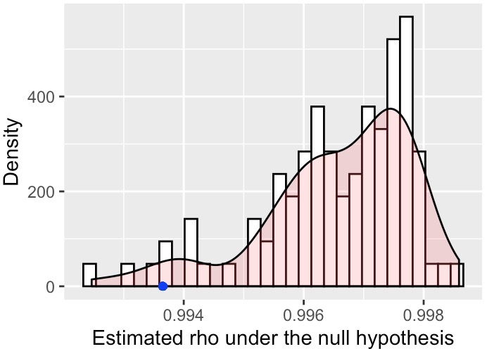
(a) $H_{0}:\textbf{X}_{\text{Young}}=\textbf{X}_{\text{Mid}}$.
$T_{n}=0.9937$ and $p$-value is 0.04.

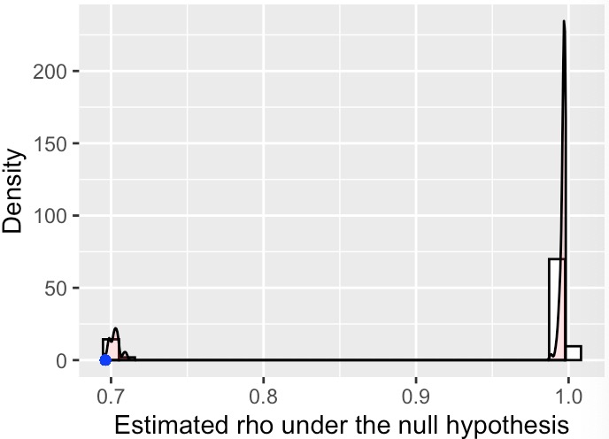
(b) $H_{0}:\textbf{X}_{\text{Mid}}=\textbf{X}_{\text{Old}}$.
$T_{n}=0.6963$ and $p$-value is 0.01.

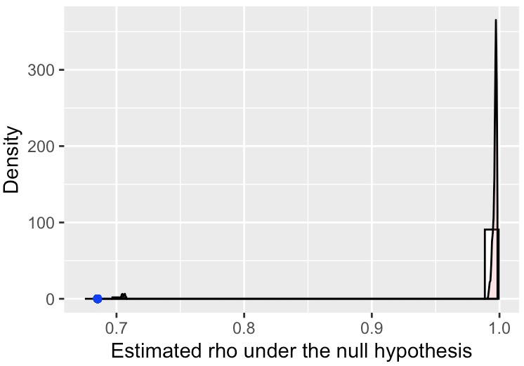
(c) $H_{0}:\textbf{X}_{\text{Young}}=\textbf{X}_{\text{Old}}$.
$T_{n}=0.6851$ and $p$-value is 0.

Figure 1: Density Plot of Estimated Test Statistic Under Different $H_{0}$.

The $p$-values given in Figure 1 are marginal $p$-values and had not been corrected for multiple comparisons. Applying Bonferroni correction with significance level $0.05/3\approx 0.017$, we fail to reject the null hypothesis that there is no difference between the young and the middle-aged group; the value of the test statistic for this comparison is $T\approx 0.994$. In contrasts, we reject the null hypothesis for the comparison of young against old and the comparison of middle-aged against old. The histograms in Figure 1 also indicate that the empirical distribution of the permutation test statistic for comparing young and the middle-aged group is tightly concentrated at $1$, once again suggesting that these two groups are quite similar.

5.2 Application 2: epileptogenic data on recording region and brain state

The second application is on networks constructed from epileptogenic recordings of patients with epileptic seizure [Andrzejak et al., 2001]. The data is available from UCI Machine Learning Repository (http://archive.ics.uci.edu/ml/datasets.php). There are $500$ subjects whose brain activity was recorded, with the epileptogenic recording of each person being divided into $23$ one-second snapshots containing $178$ time points. The data is arranged as a matrix with $23\times 500=11500$ rows and $178$ columns. The $11500$ observations are classified into five classes; these classes are numbered from $1$ through $5$ and correspond to recordings with seizure activity, an area with tumour, a healthy brain area, subject with eyes open and subject with eyes closed. It was noted in [Andrzejak et al., 2001] that all subjects whose recordings are classified as classes $2$ through $5$ are subjects who did not have epileptic seizure and that only subjects in class $1$ have epileptic seizure. Most analysis of this data have thus been binary classification, namely discriminating class $1$ with epileptic seizure against the rest.

We constructed networks by thresholding the autocorrelation matrices of the epileptogenic data using a procedure similar to that in [Ghoshdastidar and von Luxburg, 2018]. Each class is randomly divided into four parts with equal size. We then compute the autocorrelation matrices for each part and set the diagonal elements to be 0. Unweighted adjacency matrices are then obtained by thresholding the largest $10\%$ of the correlation entries to $1$ with the remaining entries being $0$. The above steps result in $20$ adjacency matrices, with $4$ from each class. Each adjacency matrix corresponds to a graph on $n=178$ vertices.

We then compare, using our test procedure, the graphs from class $1$ against the graphs from class $j\geq 2$. The results are summarized in Table 5. The $p$-values in the table are calculated using permutation test. We see from Table 5 that class $1$ is significantly different from the remaining classes and that this difference is not too sensitive to the choice of dimension $K$ in the singular value thresholding step.

Table 5: $p$-values for epileptogenic correlation networks.

$K$	$A_{1}$ vs $A_{1}$	$A_{1}$ vs $A_{2}$	$A_{1}$ vs $A_{3}$	$A_{1}$ vs $A_{4}$	$A_{1}$ vs $A_{5}$
2	0.80	0.99	0.12	0.04	0.01
3	0.80	0.72	0.01	0.00	0.29
4	0.79	0.01	0.00	0.04	0.01
5	0.88	0.01	0.00	0.00	0.01
6	0.80	0.04	0.00	0.01	0.02
7	0.94	0.03	0.00	0.01	0.02
8	0.83	0.05	0.00	0.00	0.03

6 Discussions

In summary, the test statistic constructed based on universal singular value thresholding and Spearman’s rank correlation coefficient yields a valid and consistent test procedure for testing whether two latent distance random graphs on the same vertex set have the similar generating latent positions. A few related questions will be left for future research.

Firstly, for the two-sample hypothesis test we study, one can also develop test statistics using other techniques, for example, isotonic regression. As we briefly introduced in Section 2, when the null hypothesis is true then there exists a monotone function $f$ such that $p_{ij}=f(q_{ij})$. Thus, given graphs from the latent distance model, we can first estimate $\hat{P}$ and $\hat{Q}$ and then fit a regression model of the form $\hat{p}_{ij}=f(\hat{q}_{ij})+\epsilon_{ij}$ for some nonparametric function $f$. The two-sample testing problem can then be reformulated as testing for whether $f$ is monotone. It appears, however, that testing for monotonicity against a general alternative is still an open problem in nonparametric regression.

The second question concerns the rate of convergence of our test statistic and the class of alternatives for which the test procedure is consistent against. In particular Theorem 3.3 shows that the test procedure is consistent for class of alternatives where the distance between the collections of latent positions diverges with rate $\Omega(n^{1/2})$. Relaxing this condition will require careful analysis of the estimation error in the singular value thresholding procedure as well as convergence rate for non-metric embedding.

Finally, the critical region for our test procedures are determined using resampling methods such as permutation test or bootstrapping graphs from the estimated edge probabilities. The validity of these resampling techniques are justified by the empirical simulation studies as well as real data analysis. Nevertheless, our test procedure could be more robust if we are able to derive the limiting distribution of the test statistic and thereby obtain approximate critical values. We surmise, however, that this will be a challenging problem. Indeed, while the limiting variance and distribution of Spearman’s rank correlation in the case of independent and identically distributed data are well known, see e.g., [Kendall, 1948] and [Ruymgaart et al., 1972], the entries in our estimates $\hat{P}$ and $\hat{Q}$ are not independent, and furthermore the original entries of $P$ and $Q$ are not identically distributed.

7 Supplementary

This supplementary file contains proofs of the theoretical results in the main paper and an additional simulation experiment.

7.1 Proofs

In this section, we will show the detailed proof of Theorem 3.1 and 3.2. Before that, let us recall the necessary notations and assumptions given in Section 3 of the main paper.

Notations. Let $n$ be the number of vertices. $P\in\mathbb{R}^{n\times n}$ is the binary symmetric edge-probability matrix. $R(P)$ is a symmetric matrix measuring ranks corresponding to $P$. Denote universal singular value thresholding estimated edge-probability matrix as $\hat{P}$. For $\eta>0$ and $(\eta^{2}\rho)^{-1}=o(n)$, we define the discretization as $\tilde{p}_{ij}=\left\lceil\hat{p}_{ij}/\eta\right\rceil\times\eta$. Let $\|\cdot\|_{F}$ be the Frobenius norm.

Assumptions. We made several required assumptions as follows.

1. As $n\to\infty$, for any $\epsilon>0$, there exists $\delta>0$ such that $[0,1)$ can be partitioned into the union of intervals of the form $[(k-1)\delta,k\delta)$ for $k=1,...,\lceil 1/\delta\rceil$, such that, for any $k$, one of the following two conditions holds almost surely:

   1. Either the number of $ij$ pairs with $i<j$ and $p_{ij}\in[(k-1)\delta,k\delta)$ is at most $n(n-1)\epsilon/2$.

   2. Or if the number of $ij$ pairs with $i<j$ and $p_{ij}\in[(k-1)\delta,k\delta)$ exceeds $n(n-1)\epsilon/2$, then they are all equal for $p_{ij}\in[(k-1)\delta,k\delta)$.

2. Define $\hat{\sigma}\{R(P)\}=\Bigl{[}{n\choose 2}^{-1}\sum_{i<j}\Bigl{\{}R(p_{ij})-{n\choose 2}^{-1}\sum_{i<j}R(p_{ij})\Bigr{\}}^{2}\Bigr{]}^{1/2}$ and $\hat{\sigma}\{R(Q)\}$ similarly. It holds that $\hat{\sigma}\{R(P)\}=\Omega(n^{2})$ and $\hat{\sigma}\{R(Q)\}=\Omega(n^{2})$.

3. The link functions $h$ and $g$ are infinitely many times differentiable.

4. Every edge is observed independently with probability $\rho\in(0,1]$, where there exists a positive constant $C$ such that $n\rho\geq C\log n$.

5. There exists a constant $c>0$ independent of $\delta$ such that $|\{(i,j):p_{ij}\in[(k-1)\delta,k\delta]\}|\leq c\cdot\delta{\tbinom{n}{2}}$.

6. Let $U\subset\mathbb{R}^{d}$ and $V\subset\mathbb{R}^{d}$, be bounded and connected sets. Let $\Omega_{n}=\{{x}_{1},...,{x}_{n}\}\subset U$ and $\Xi_{n}=\{y_{1},y_{2},\dots,y_{n}\}\subset V$. Then $\lim_{n\rightarrow\infty}\Omega_{n}$ is dense in $U$ and $\lim_{n\rightarrow\infty}\Xi_{n}$ is dense in $V$. Furthermore, for any $\epsilon>0$ there exists $\delta_{U}=\delta_{U}(\epsilon)>0$ and $\delta_{V}=\delta_{V}(\epsilon)>0$ such that

   $$n^{-1}\liminf|B(x,\epsilon)\cap\Omega_{n}|\geq\delta_{U},\qquad\text{for all $x\in U$}.$$

   $$n^{-1}\liminf|B(y,\epsilon)\cap\Xi_{n}|\geq\delta_{V},\qquad\text{for all $y\in V$}.$$

   Here $B(x,\epsilon)$ denote the ball of radius $\epsilon$ around $x\in\mathbb{R}^{d}$.

We now prove Theorem 3.1.

Theorem 3.1 Assume Assumptions 1–4 hold. Then for sufficiently large $n$,

$$T_{n}(\tilde{P},\tilde{Q})-T_{n}(P,Q)=o_{p}(1).$$

Here $\tilde{P}$ and $\tilde{Q}$ are the $\eta$-discretization of $\hat{P}$ and $\hat{Q}$ with $(\eta^{2}\rho)^{-1}=o(n)$ as $n\rightarrow\infty$.

of Theorem 3.1.

From Theorem 1 in [Xu, 2018], along with the conditions in Assumptions 3 and 4, we have

$$\|\hat{P}-P\|^{2}_{F}=O_{p}\Bigl{\{}\frac{n\log^{d}(n\rho)}{\rho}\Bigr{\}},$$ (7.1)

where $d$ is the dimension of latent positions. Let $\eta>0$ be such that $(\eta^{2}\rho)^{-1}=o(n)$. Define $S=\Bigl{\{}(i,j):|\hat{p}_{ij}-p_{ij}|>\eta\Bigr{\}}$. Then by (7.1), we have

$$|S|=O\Bigl{[}n\Bigl{\{}\log^{d}(n\rho)\Bigr{\}}/(\eta^{2}\rho)\Bigr{]}=o(n^{2}).$$

Recall that our test statistic, using the true $P$ and $Q$, is

$$T_{n}(P,Q) =\frac{\mathrm{cov}\{R(P),R(Q)\}}{\hat{\sigma}\{R(P)\}\hat{\sigma}\{R(Q)\}},$$

where

$$\mathrm{cov}\{R(P),R(Q)\} =\tbinom{n}{2}^{-1}\sum_{i,j}R(p_{ij})R(q_{ij})-\Bigl{\{}\tbinom{n}{2}^{-1}\sum_{i,j}R(p_{ij})\Bigr{\}}\times\Bigl{\{}\tbinom{n}{2}^{-1}\sum_{i,j}R(q_{ij})\Bigr{\}},$$

$$\hat{\sigma}\{R(P)\} =\Bigl{[}\tbinom{n}{2}^{-1}\sum_{i,j}\Bigl{\{}R(p_{ij})-\tbinom{n}{2}^{-1}\sum_{i,j}R(p_{ij})\Bigr{\}}^{2}\Bigr{]}^{1/2},$$

$$\hat{\sigma}\{R(Q)\} =\Bigl{[}\tbinom{n}{2}^{-1}\sum_{i,j}\Bigl{\{}R(q_{ij})-\tbinom{n}{2}^{-1}\sum_{i,j}R(q_{ij})\Bigr{\}}^{2}\Bigr{]}^{1/2}.$$

The test statistic $T_{n}(\tilde{P},\tilde{Q})$ using the discretized estimates is defined analogously. We then have

$$\begin{split}T_{n}(\tilde{P},\tilde{Q})-T_{n}(P,Q)&=\frac{\mathrm{cov}\{R(\tilde{P}),R(\tilde{Q})\}}{\hat{\sigma}\{R(\tilde{P})\}\hat{\sigma}\{R(\tilde{Q})\}}-\frac{\mathrm{cov}\{R(P),R(Q)\}}{\hat{\sigma}\{R(P)\}\hat{\sigma}\{R(Q)\}}\\ &=\underbrace{\frac{\mathrm{cov}\{R(\tilde{P}),R(\tilde{Q})\}-\mathrm{cov}\{R(P),R(Q)\}}{\hat{\sigma}\{R(\tilde{P})\}\hat{\sigma}\{R(\tilde{Q})\}}}_{\text{Part I}}\\ &+\underbrace{\mathrm{cov}\{R(P),R(Q)\}\Bigl{[}\frac{1}{\hat{\sigma}\{R(\tilde{P})\}\hat{\sigma}\{R(\tilde{Q})\}}-\frac{1}{\hat{\sigma}\{R(P)\}\hat{\sigma}\{R(Q)\}}\Bigr{]}}_{\text{Part II}}.\end{split}$$

We control Part I and Part II via the following two lemmas.

Lemma 1.

Under assumptions 1,3 and 4, for any $\epsilon>0$, there exists a positive constant $C$ such that

$$\Bigl{|}\sum_{i<j}R(\tilde{p}_{ij})\sum_{i<j}R(\tilde{q}_{ij})-\sum_{i<j}R(p_{ij})\sum_{i<j}R(q_{ij})\Bigr{|}\leq Cn^{8}\epsilon.$$

Lemma 2.

Under assumptions 1,3 and 4, for any $\epsilon>0$, there exists a positive constant $C$ such that

$$\Bigl{|}\hat{\sigma}^{2}\{R(\tilde{P})\}-\hat{\sigma}^{2}\{R(P)\}\Bigr{|}\leq Cn^{4}\epsilon.$$

Suppose Lemma 1 and 2 are valid then we can complete the proof of Theorem 3.1. Lemma 1 is used to control the numerator in each part while Lemma 2 is for the denominator. For any $\epsilon>0$, we have $\mathrm{cov}\{R(\tilde{P}),R(\tilde{Q})\}-\mathrm{cov}\{R(P),R(Q)\}=O_{p}(n^{4}\epsilon)$ by Lemma 1 and $\hat{\sigma}\{R(\tilde{P})\}=\hat{\sigma}\{R(P)\}+O_{p}(n^{2}\epsilon^{1/2})$ by Lemma 2. Under Assumption 2, $\hat{\sigma}\{R(P)\}=\Omega(n^{2})$. Thus, it holds that $\hat{\sigma}\{R(\tilde{P})\}=\Omega_{p}(n^{2})$. Similarly, $\hat{\sigma}\{R(\tilde{Q})\}=\Omega_{p}(n^{2})$. Therefore, we have

$$\text{Part I}=\frac{\mathrm{cov}\{R(\tilde{P}),R(\tilde{Q})\}-\mathrm{cov}\{R(P),R(Q)\}}{\hat{\sigma}\{R(\tilde{P})\}\hat{\sigma}\{R(\tilde{Q})\}}=O_{p}({\epsilon}^{1/2}).$$

Then,

$$\text{Part II}= \mathrm{cov}\{R(P),R(Q)\}\Bigl{[}\frac{1}{\hat{\sigma}\{R(\tilde{P})\}\hat{\sigma}\{R(\tilde{Q})\}}-\frac{1}{\hat{\sigma}\{R(P)\}\hat{\sigma}\{R(Q)\}}\Bigr{]}$$

$$\leq \hat{\sigma}\{R(P)\}\hat{\sigma}\{R(Q)\}\frac{\hat{\sigma}\{R(P)\}\hat{\sigma}\{R(Q)\}-\hat{\sigma}\{R(\tilde{P})\}\hat{\sigma}\{R(\tilde{Q})\}}{\hat{\sigma}\{R(\tilde{P})\}\hat{\sigma}\{R(\tilde{Q})\}\hat{\sigma}\{R(P)\}\hat{\sigma}\{R(Q)\}}$$

$$= \frac{\hat{\sigma}\{R(P)\}\hat{\sigma}\{R(Q)\}-\hat{\sigma}\{R(\tilde{P})\}\hat{\sigma}\{R(\tilde{Q})\}}{\hat{\sigma}\{R(\tilde{P})\}\hat{\sigma}\{R(\tilde{Q})\}}$$

$$= \frac{\Bigl{[}\hat{\sigma}\{R(P)\}-\hat{\sigma}\{R(\tilde{P})\}\Bigr{]}\hat{\sigma}\Bigl{\{}R(Q)\Bigr{]}+\hat{\sigma}\{R(\tilde{P})\}\Bigl{[}\hat{\sigma}\{R(Q)\}-\hat{\sigma}\{R(\tilde{Q})\}\Bigr{]}}{\Omega_{p}(n^{4})}$$

$$= \frac{O_{p}(n^{2}\epsilon^{1/2})O(n^{2})+\Bigl{\{}O_{p}(n^{2}\epsilon^{1/2})+O(n^{2})\Bigr{\}}O_{p}(n^{2}\epsilon^{1/2})}{\Omega_{p}(n^{4})}$$

$$= \frac{2O_{p}(n^{2}\epsilon^{1/2})O(n^{2})+O_{p}(n^{4}\epsilon)}{\Omega_{p}(n^{4})}=O_{p}({\epsilon}^{1/2}).$$

Combining the above bounds yields

$$T_{n}(\tilde{P},\tilde{Q})-T_{n}(P,Q)=O_{p}({\epsilon}^{1/2}).$$

Since $\epsilon>0$ is arbitrary, we have $T_{n}(\tilde{P},\tilde{Q})-T_{n}(P,Q)=o_{p}(1)$ as desired. ∎

We now prove Lemmas 1 and 2. The proof of Lemma 1 depends on the following result.

Lemma 3.

Under assumptions 1,3 and 4, for any $\epsilon>0$, there exists a positive constant $C$ such that

$$\Bigl{|}\sum_{i<j}\Bigl{\{}R(\tilde{p}_{ij})R(\tilde{q}_{ij})-R(p_{ij})R(q_{ij})\Bigr{\}}\Bigr{|}\leq Cn^{6}\epsilon.$$

of Lemma 3.

Our proof is based on bounding $|R(\tilde{p}_{rs})-R(p_{rs})|$ and $|R(\tilde{q}_{rs})-R(q_{rs})|$. First consider pairs $(i,j)\notin S$. Since $|\hat{p}_{ij}-p_{ij}|\leq\eta$ and $|\tilde{p}_{ij}-\hat{p}_{ij}|\leq\eta$, we have $|\tilde{p}_{ij}-p_{ij}|\leq 2\eta$. Now suppose that $\tilde{p}_{ij}\leq x$. Then $p_{ij}\leq x+2\eta$. We therefore have

$$|\{(i,j):\tilde{p}_{ij}\leq x\}|\leq|\{(i,j):p_{ij}\leq x+2\eta\}|,\quad|\{(i,j):\tilde{p}_{ij}<x\}|\geq|\{(i,j):p_{ij}<x-2\eta\}|.$$

Thus, for a given pair $(r,s)\notin\mathcal{S}$, we have

$$R(\tilde{p}_{rs}) \leq|\{(i,j):\tilde{p}_{ij}\leq\tilde{p}_{rs}\}|\leq|\{(i,j):p_{ij}\leq\tilde{p}_{rs}+2\eta\}|\leq|\{(i,j):p_{ij}\leq p_{rs}+4\eta\}|$$

$$\leq R(p_{rs})+5\tbinom{n}{2}\epsilon.$$

A similar argument shows, for $(r,s)\not\in\mathcal{S}$,

$$R(\tilde{p}_{rs}) \geq|\{(i,j):\tilde{p}_{ij}<\tilde{p}_{rs}\}|\geq|\{(i,j):p_{ij}<\tilde{p}_{rs}-2\eta\}|\geq|\{(i,j):p_{ij}<p_{rs}-4\eta\}|$$

$$=|\{(i,j):p_{ij}\leq p_{rs}-4\eta\}|-|\{(i,j):p_{ij}=p_{rs}-4\eta\}|$$

$$\geq R(p_{rs})-4\tbinom{n}{2}\epsilon-\tbinom{n}{2}\epsilon=R(p_{rs})-5\tbinom{n}{2}\epsilon.$$

Therefore, for $(r,s)\notin S$ and any $\epsilon>0$, we have

$$|R(\tilde{p}_{rs})-R(p_{rs})|\leq 5\tbinom{n}{2}\epsilon.$$ (7.2)

A similar argument yields

$$|R(\tilde{q}_{rs})-R(q_{rs})|\leq 5\tbinom{n}{2}\epsilon.$$ (7.3)

By applying (7.2) and (7.3), for $(i,j)\notin S$ and any $\epsilon>0$, it holds that

$$\Bigl{|}R(\tilde{p}_{ij})R(\tilde{q}_{ij})-R(p_{ij})R(q_{ij})\Bigr{|}$$

$$\leq\Bigl{|}R(\tilde{p}_{ij})-R(p_{ij})\Bigr{|}R(q_{ij})+\Bigl{|}R(\tilde{q}_{ij})-R(q_{ij})\Bigr{|}R(p_{ij})+\Bigl{|}R(\tilde{p}_{ij})-R(p_{ij})\Bigr{|}\Bigl{|}R(\tilde{q}_{ij})-R(q_{ij})\Bigr{|}$$

$$\leq 5\tbinom{n}{2}\epsilon\times R(q_{ij})+5\tbinom{n}{2}\epsilon\times R(p_{ij})+25\tbinom{n}{2}^{2}\epsilon^{2}.$$

Now consider $(i,j)\in S$. Then by assumption 3 and 4,

$$\sum_{(i,j)\in S}\Bigl{|}R(\tilde{p}_{ij})R(\tilde{q}_{ij})-R(p_{ij})R(q_{ij})\Bigr{|}\leq O_{p}(|S|\cdot n^{4})=o_{p}(n^{6}).$$

Therefore, for any $1\leq i<j\leq n$, there exists a positive constant $C$ such that

$$\Bigl{|}\sum_{1\leq i<j\leq n}R(\tilde{p}_{ij})R(\tilde{q}_{ij})-R(p_{ij})R(q_{ij})\Bigr{|}$$

$$\leq\sum_{(i,j)\notin S}\Bigl{|}R(\tilde{p}_{ij})R(\tilde{q}_{ij})-R(p_{ij})R(q_{ij})\Bigr{|}+\sum_{(i,j)\in S}\Bigl{|}R(\tilde{p}_{ij})R(\tilde{q}_{ij})-R(p_{ij})R(q_{ij})\Bigr{|}$$

$$\leq 5\tbinom{n}{2}\epsilon\sum_{(i,j)\notin S}R(p_{ij})+5\tbinom{n}{2}\epsilon\sum_{(i,j)\notin S}R(q_{ij})+25\tbinom{n}{2}^{3}\epsilon^{2}+o_{p}(n^{6})$$

$$\leq Cn^{6}\epsilon$$

as desired. ∎

of Lemma 1.

By (7.2) and (7.3),

$$\Bigl{|}\sum_{(i,j)\notin S}R(\tilde{p}_{ij})\sum_{(i,j)\notin S}R(\tilde{q}_{ij})-\sum_{(i,j)\notin S}R(p_{ij})\sum_{(i,j)\notin S}R(q_{ij})\Bigr{|}$$

$$\leq \Bigl{|}\sum_{(i,j)\notin S}R(\tilde{p}_{ij})-\sum_{(i,j)\notin S}R(p_{ij})\Bigr{|}\sum_{(i,j)\notin S}R(q_{ij})+\Bigl{|}\sum_{(i,j)\notin S}R(\tilde{q}_{ij})-\sum_{(i,j)\notin S}R(q_{ij})\Bigr{|}\sum_{(i,j)\notin S}R(p_{ij})$$

$$+\Bigl{|}\sum_{(i,j)\notin S}R(\tilde{p}_{ij})-\sum_{(i,j)\notin S}R(p_{ij})\Bigr{|}\Bigl{|}\sum_{(i,j)\notin S}R(\tilde{q}_{ij})-\sum_{(i,j)\notin S}R(q_{ij})\Bigr{|}$$

$$\leq \sum_{(i,j)\notin S}\Bigl{|}R(\tilde{p}_{ij})-R(p_{ij})\Bigr{|}\sum_{(i,j)\notin S}R(q_{ij})+\sum_{(i,j)\notin S}\Bigl{|}R(\tilde{q}_{ij})-R(q_{ij})\Bigr{|}\sum_{(i,j)\notin S}R(p_{ij})$$

$$+\sum_{(i,j)\notin S}\Bigl{|}R(\tilde{p}_{ij})-R(p_{ij})\Bigr{|}\sum_{(i,j)\notin S}\Bigl{|}R(\tilde{q}_{ij})-R(q_{ij})\Bigr{|}$$

$$= 10{\tbinom{n}{2}}^{2}\epsilon\cdot O(n^{4})+25{\tbinom{n}{2}}^{4}\epsilon^{2}\leq Cn^{8}\epsilon.$$

For $(i,j)\in S$, under assumption 3 and 4, it holds that

$$\Bigl{|}\sum_{(i,j)\in S}R(\tilde{p}_{ij})\sum_{(i,j)\in S}R(\tilde{q}_{ij})-\sum_{(i,j)\in S}R(p_{ij})\sum_{(i,j)\in S}R(q_{ij})\Bigr{|}\leq O_{p}(|S|^{2}n^{4})=o_{p}(n^{8}).$$

Therefore, for $1\leq i<j\leq n$ and any $\epsilon>0$, there exists a positive constant $C$ such that

$$\Bigl{|}\sum_{i<j}R(\tilde{p}_{ij})\sum_{i<j}R(\tilde{q}_{ij})-\sum_{i<j}R(p_{ij})\sum_{i<j}R(q_{ij})\Bigr{|}\leq Cn^{8}\epsilon.$$

∎

of Lemma 2.

By (7.2), for $(i,j)\notin S$ and any $\epsilon>0$, we have

$$\sum_{(i,j)\notin S}\Bigl{|}R^{2}(\tilde{p}_{ij})-R^{2}(p_{ij})\Bigr{|} \leq 2\sum_{(i,j)\notin S}\Bigl{|}R(\tilde{p}_{ij})-R(p_{ij})\Bigr{|}R(p_{ij})+\sum_{(i,j)\notin S}\Bigl{|}R(\tilde{p}_{ij})-R(p_{ij})\Bigr{|}^{2}$$

$$\leq 10{\tbinom{n}{2}}\epsilon\cdot\sum_{(i,j)\notin S}R(p_{ij})+25{\tbinom{n}{2}}^{3}\epsilon^{2}$$

$$=10{\tbinom{n}{2}}\epsilon\cdot O(n^{4})+25{\tbinom{n}{2}}^{3}\epsilon^{2}=Cn^{6}\epsilon.$$ (7.4)

Consider $(i,j)\in S$. Similarly, by assumption 3 and 4, it holds that

$$\sum_{(i,j)\in S}\Bigl{|}R^{2}(\tilde{p}_{ij})-R^{2}(p_{ij})\Bigr{|} \leq 2\sum_{(i,j)\in S}\Bigl{|}R(\tilde{p}_{ij})-R(p_{ij})\Bigr{|}R(p_{ij})+\sum_{(i,j)\in S}\Bigl{|}R(\tilde{p}_{ij})-R(p_{ij})\Bigr{|}^{2}$$

$$=O_{p}(|S|n^{4})=o_{p}(n^{6}).$$ (7.5)

Thus, combining (7.1) and (7.1), for $1\leq i<j\leq n$ and any $\epsilon>0$, there exists $C>0$ such that

$$\sum_{i<j}\Bigl{|}R^{2}(\tilde{p}_{ij})-R^{2}(p_{ij})\Bigr{|}\leq Cn^{6}\epsilon.$$ (7.6)

Following the similar procedure of deriving (7.6), it is easy to show for any $\epsilon>0$, there exists $C>0$ such that

$$\Bigl{|}\Bigl{\{}{\tbinom{n}{2}}^{-1}\sum_{i<j}R(\tilde{p}_{ij})\Bigr{\}}^{2}-\Bigl{\{}{\tbinom{n}{2}}^{-1}\sum_{i<j}R(p_{ij})\Bigr{\}}^{2}\Bigr{|}\leq Cn^{4}\epsilon.$$ (7.7)

By (7.6) and (7.7), for any $\epsilon>0$, there exists a positive constant $C$ such that

$$\Bigl{|}{\tbinom{n}{2}}^{-1}\sum_{i<j}\Bigl{\{}R(\tilde{p}_{ij})-\sum_{i<j}R(\tilde{p}_{ij})\Bigr{\}}^{2}-{\tbinom{n}{2}}^{-1}\sum_{i<j}\Bigl{\{}R(p_{ij})-{\tbinom{n}{2}}^{-1}\sum_{i<j}R(p_{ij})\Bigr{\}}^{2}\Bigr{|}$$

$$\leq {\tbinom{n}{2}}^{-1}\sum_{i<j}\Bigl{|}R^{2}(\tilde{p}_{ij})-R^{2}(p_{ij})\Bigr{|}+\Bigl{|}\Bigl{\{}{\tbinom{n}{2}}^{-1}\sum_{i<j}R(\tilde{p}_{ij})\Bigr{\}}^{2}-\Bigl{\{}{\tbinom{n}{2}}^{-1}\sum_{i<j}R(p_{ij})\Bigr{\}}^{2}\Bigr{|}$$

$$\leq Cn^{4}\epsilon.$$

∎

Then we will prove Theorem 3.2, which requires the following lemma.

Lemma 4.

Given $X=({x}_{1},...,{x}_{n})^{\top}\in\mathbb{R}^{n\times d}$ and $Y=({y}_{1},...,{y}_{n})^{\top}\in\mathbb{R}^{n\times d}$. Define $P=(p_{ij})\in\mathbb{R}^{n\times n}$ and $Q=(q_{ij})\in\mathbb{R}^{n\times n}$, where $p_{ij}=h(\|{x}_{i}-{x}_{j}\|)$ and $q_{ij}=g(\|{y}_{i}-{y}_{j}\|)$ for some monotone decreasing functions $h,g$ from $\mathbb{R}$ onto $\mathbb{R}$. Under Assumption 3 and 6, if $\lim_{n\to\infty}T_{n}(P,Q)=1$ then there exists a sequence of monotone increasing functions $f_{n}$ from $\mathbb{R}$ onto $\mathbb{R}$ such that, as $n\to\infty$,

$$\max_{i,j}\Bigl{|}\|{y}_{i}-{y}_{j}\|-f_{n}\Bigl{(}\|{x}_{i}-{x}_{j}\|\Bigr{)}\Bigr{|}\rightarrow 0.$$

of Lemma 4.

Since $T_{n}(P,Q)\rightarrow 1$, for any $\epsilon>0$ there exists a universal constant $C$ and a $n_{0}=n_{0}(\epsilon)$ such that if $n\geq n_{0}$ then the number of pairs $\{i,j\}$ with $|R(p_{ij})-R(q_{ij})|\geq\tbinom{n}{2}\epsilon$ is at most $C\tbinom{n}{2}\epsilon$. Let $\mathcal{S}$ be the set of pairs satisfying

$$|R(p_{ij})-R(q_{ij})|<\tbinom{n}{2}\epsilon.$$ (7.8)

Define rank functions normalized by ${n\choose 2}$ as $\tilde{R}_{p},\tilde{R}_{q}:[0,1]\mapsto[0,1]$. We can rewrite (7.8) as

$$\Bigl{|}\tilde{R}_{q}\Bigl{\{}g(\|{y}_{i}-{y}_{j}\|)\Bigr{\}}-\tilde{R}_{p}\Bigl{\{}h(\|{x}_{i}-{x}_{j}\|)\Bigr{\}}\Bigr{|}<C\epsilon.$$

According to Assumption 3, $\tilde{R}_{q}\circ g$ is uniformly continuous. Thus, for all $\{i,j\}\in\mathcal{S}$,

$$\|{y}_{i}-{y}_{j}\| \in\Bigl{[}g^{-1}\circ\tilde{R}_{q}^{-1}\Bigl{\{}\tilde{R}_{p}\circ h(\|{x}_{i}-{x}_{j}\|)\pm C\epsilon\Bigr{\}}\Bigr{]}$$

$$\in\Bigl{[}g^{-1}\circ\tilde{R}_{q}^{-1}\Bigl{\{}\tilde{R}_{p}\circ h(\|{x}_{i}-{x}_{j}\|)\Bigr{\}}\pm\epsilon_{1}\Bigr{]},$$

where $\epsilon_{1}>0$ depends on $g^{-1}\circ\tilde{R}_{q}^{-1}$, $C$ and $\epsilon$. Also, $\epsilon_{1}\rightarrow 0$ as $\epsilon\rightarrow 0$ due to the uniform continuity of $\tilde{R}_{q}\circ g$. Define a sequence of functions $f_{n}=g^{-1}\circ\tilde{R}_{q}^{-1}\circ\tilde{R}_{p}\circ h$. We then have, for all $\{i,j\}\in\mathcal{S}$,

$$\max_{i,j}\Bigl{|}\|{y}_{i}-{y}_{j}\|-f_{n}\Bigl{(}\|{x}_{i}-{x}_{j}\|\Bigr{)}\Bigr{|}\to 0,$$

as $n\to\infty$.

We next consider the pairs $\{i,j\}\not\in\mathcal{S}$. Suppose first that there exists a pair $\{k,\ell\}\in\mathcal{S}$ such that both $R(p_{ij})-R(p_{k\ell})\leq\tbinom{n}{2}\epsilon$ and $R(q_{ij})-R(q_{k\ell})\leq\tbinom{n}{2}\epsilon$. Then by the continuity and monotonicity of $f_{n}$, we have

$$\|y_{i}-y_{j}\|\in\Bigl{(}\|y_{k}-y_{\ell}\|\pm C\epsilon_{1}\Bigr{)}\subset\Bigl{(}f(\|x_{k}-x_{\ell}\|\pm\epsilon)\pm C\epsilon_{1}\Bigr{)}$$

and by taking $\epsilon$ (and hence $\epsilon_{1}$) sufficiently small, we have

$$\|y_{i}-y_{j}\|-f_{n}(\|x_{i}-x_{j}\|)\rightarrow 0$$

as $n\rightarrow\infty$.

It remains to consider the pairs $\{i,j\}\not\in\mathcal{S}$ such that either $|R(p_{ij})-R(p_{k\ell})|\geq\tbinom{n}{2}\epsilon$ for all $\{k,\ell\}\in\mathcal{S}$ or that $|R(q_{ij})-R(q_{k\ell})|\geq\tbinom{n}{2}\epsilon$ for all $\{k,\ell\}\in\mathcal{S}$. Suppose $|R(p_{ij})-R(p_{k\ell})|\geq\tbinom{n}{2}\epsilon$ for all $\{k,\ell\}\in\mathcal{S}$. Then there exists a $\delta>0$ such that for all $i^{\prime},j^{\prime}$, if

$$\|x_{i^{\prime}}-x_{i}\|\leq\delta,\quad\|x_{j^{\prime}}-x_{j}\|\leq\delta$$

then $|R(p_{i^{\prime}j^{\prime}})-R(p_{ij})|\leq\tbinom{n}{2}\epsilon$, i.e., we have $\{i^{\prime},j^{\prime}\}\not\in\mathcal{S}$. That is to say, points $x_{i^{\prime}}$ “close” to $x_{i}$ and $x_{j^{\prime}}$ “close“ to $x_{j}$ will have distance $\|x_{i^{\prime}}-x_{j^{\prime}}\|$ “close” to $\|x_{i}-x_{j}\|$ and hence the ranks of $p_{i^{\prime}j^{\prime}}$ and $p_{ij}$ are “close”. Assumption 6 then implies that number of points in $B(x_{i},\delta)$ is of order $\Omega(n)$ as $n\rightarrow\infty$ and since $|\mathcal{S}^{c}|$ has at most $C\tbinom{n}{2}\epsilon$ elements, the vertex covering number for $\mathcal{S}^{c}$ is of order $O(n\epsilon^{1/2})$ as $n\rightarrow\infty$. We can then remove these vertices from consideration. We repeat the same procedure for $Q$.

In summary, if $T_{n}(P,Q)\rightarrow 1$ then there is a subset of $\mathcal{T}$ rows of both $X$ and $Y$ such that $|\mathcal{T}|=n-O(n\epsilon^{1/2})$ and

$$\|y_{i}-y_{j}\|-f_{n}(\|x_{i}-x_{j}\|)\rightarrow 0,\quad i,j\in\mathcal{T}.$$

As $\epsilon>0$ is arbitrary, we can have $|\mathcal{T}|=n-o(n)$ for sufficiently large $n$.

Once again, by Assumption $6$, any sequence of $n-o(n)$ elements $\{x_{i}\colon i\in\mathcal{T}\}$ will be dense in $U$ as $n\rightarrow\infty$, and the corresponding $\{y_{i}\colon i\in\mathcal{T}\}$ will be dense in $V$. We therefore have,

$$\max_{ij}\Bigl{|}\|y_{i}-y_{j}\|-f_{n}(\|x_{i}-x_{j}\|)\Bigr{|}\longrightarrow 0$$

as $n\rightarrow\infty$ as desired.

∎

Theorem 3.2 Under Assumption 3 and 6, if $T_{n}(P,Q)\to 1$ as $n\to\infty$, it holds that there exists $s\in\mathbb{R}$, orthogonal $W\in\mathbb{R}^{d\times d}$ and ${t}\in\mathbb{R}^{d}$ such that

$$\|X-sYW-1t^{\top}\|_{F}=o(n^{1/2}).$$

of Theorem 3.2.

Let $\phi_{n}:\Xi_{n}\mapsto\Omega_{n}\subset\mathbb{R}^{d}$ be a function with values in a bounded set $\Omega_{n}=\{{x}_{1},...,{x}_{n}\}$. Let $\Xi=\lim_{n\rightarrow\infty}\Xi_{n}$.

Now take ${y}_{i},{y}_{j},{y}_{k}\in\Xi$ such that $\|{y}_{i}-{y}_{j}\|<\|{y}_{i}-{y}_{k}\|$. By definition, there is $m$ such that ${y}_{i},{y}_{j},{y}_{k}\in\Xi_{m}$. Therefore, by Lemma 4, for any $0<\epsilon\leq(\|{y}_{i}-{y}_{k}\|-\|{y}_{i}-{y}_{j}\|)/2$, there exists a $m^{\prime}\geq m$ such that $f_{n}(\|\phi_{n}({y}_{i})-\phi_{n}({y}_{j})\|)\leq f_{n}(\|\phi_{n}({y}_{i})-\phi_{n}({y}_{k})\|)$ for any $n\geq m^{\prime}$. Since $f_{n}\colon\mathbb{R}\mapsto\mathbb{R}$ is an increasing function, we have $\|\phi_{n}({y}_{i})-\phi_{n}({y}_{j})\|\leq\|\phi_{n}({y}_{i})-\phi_{n}({y}_{k})\|$ for any $n\geq m^{\prime}$.

By Lemma 2 in [arias2017some], since $\Xi_{n}\subset\mathbb{R}^{d}$ is finite and $\phi_{n}:\Xi_{n}\mapsto\Omega_{n}\subset\mathbb{R}^{d}$, where $\Omega_{n}$ is bounded, there is $N\subset\mathbb{N}$ infinite such that $\phi({y}_{i})=\lim_{n\in N}\phi_{n}({y}_{i})$ exists for all ${y}_{i}\in\Omega=\cup_{n=1}^{\infty}\Omega_{n}$.

Passing to the limit along $n\in N$ where $N$ is infinite and $N\subset\mathbb{N}$, we obtain $\|\phi({y}_{i})-\phi({y}_{j})\|\leq\|\phi({y}_{i})-\phi({y}_{k})\|$. Hence, $\phi$ is weakly isotonic on $\Omega$ and by Theorem 1 in [arias2017some], there exists a similarity transformation that coincides with $\phi$ on $\Omega$. That is, there exists constant $s>0$, orthogonal matrix $W\in\mathbb{R}^{d\times d}$ and constant vector ${t}\in\mathbb{R}^{d}$ such that as $n\to\infty$, for all pairs $(i,j)$ with $1\leq i<j\leq n$,

$$\|{x}_{i}-sW{y}_{i}-{t}\|\to 0.$$

We therefore have

$$0\leq n^{-1/2}\|X-sYW-1t^{\top}\|_{F} =\Bigl{(}n^{-1}\sum_{i=1}^{n}\|{x}_{i}-sW{y}_{i}-{t}\|^{2}\Bigr{)}^{1/2}$$

$$\leq\max_{i}\|{x}_{i}-s{y}_{i}W-{t}\|\to 0$$

as desired. ∎

7.2 Additional Simulation Study

Simulation 4: Sparsity. This simulation is designed to investigate the the influence of sparsity of networks. Set dimension of embedding $K=3$, sparsity level $\rho$ satisfying $\rho=(\gamma\log{n})/n$ where $\gamma\in\{3,5\}$, $n\in\{100,200,500,1000\}$ and significant level $\alpha=0.05$. The latent positions are set to be $Y=X+Z$ where $Z=(z_{ij})\in\mathbb{R}^{n\times 2}$ and $z_{ij}\overset{iid}{\sim}N(0,\epsilon)$ and $\epsilon\in\{0,0.02,0.1,0.2,0.5,1\}$.

Table 6: Power of the proposed test under different sparsity levels ($\alpha=0.05$).

$\rho$	$n$	$\epsilon=0$	$\epsilon=0.02$	$\epsilon=0.1$	$\epsilon=0.2$	$\epsilon=0.5$	$\epsilon=1$
$\frac{3\log{n}}{n}$	100	0.05	0.15	0.29	0.37	0.88	0.97
	200	0.05	0.15	0.01	0.64	0.96	1
	500	0.05	0.29	0.50	0.92	1	1
	1000	0.05	0.06	0.46	0.94	1	1
$\frac{5\log{n}}{n}$	100	0.05	0.05	0.14	0.59	0.87	1
	200	0.05	0.01	0.35	0.26	1	1
	500	0.05	0.07	0.33	1	1	1
	1000	0.05	0.24	1	1	1	1

Table 6 illustrates the performance of our test under different sparsity levels. Overall, it performs quite well especially in the mild sparse case with $\rho\geq 5$. When the network becomes more sparse ($\rho=3$), the proposed test is not stable in the case with minor difference ($\epsilon\leq 0.1$) while it becomes much better and more robust as the difference is relatively larger ($\epsilon\geq 0.5$) , for example, it has power 1 when $n$ is 500.

References

- [Abbe, 2017] Abbe, E. (2017). Community detection and stochastic block models: recent developments. The Journal of Machine Learning Research, 18(1):6446–6531.
- [Airoldi et al., 2008] Airoldi, E. M., Blei, D. M., Fienberg, S. E., and Xing, E. P. (2008). Mixed membership stochastic blockmodels. Journal of Machine Learning Research, 9(Sep):1981–2014.
- [Andrzejak et al., 2001] Andrzejak, R. G., Lehnertz, K., Mormann, F., Rieke, C., David, P., and Elger, C. E. (2001). Indications of nonlinear deterministic and finite-dimensional structures in time series of brain electrical activity: Dependence on recording region and brain state. Physical Review E, 64(6):061907.
- [Bollobas et al., 2007] Bollobas, B., Janson, S., and Riordan, O. (2007). The phase transition in inhomogeneous random graphs. Random Structure and Algorithms, 31:3–122.
- [Borg and Groenen, 2005] Borg, I. and Groenen, P. J. F. (2005). Moderm multidimensional scaling: Theory and Applications. Springer, 2nd edition.
- [Chatterjee, 2015] Chatterjee, S. (2015). Matrix estimation by universal singular value thresholding. The Annals of Statistics, 43(1):177–214.
- [Durante et al., 2018] Durante, D., Dunson, D. B., and Vogelstein, J. T. (2018). Bayesian inference and testing of group differences in brain networks. Bayesian Analysis, 13(1):29–58.
- [Erdős and Rényi, 1960] Erdős, P. and Rényi, A. (1960). On the evolution of random graphs. Publications of the Mathematical Institute of the Hungarian Academy of Sciences, 5(1):17–60.
- [Faskowitz et al., 2018] Faskowitz, J., Yan, X., Zuo, X.-N., and Sporns, O. (2018). Weighted stochastic block models of the human connectome across the life span. Scientific Reports, 8(1):1–16.
- [Ghoshdastidar et al., 2020] Ghoshdastidar, D., Gutzeit, M., Carpentier, A., and von Luxburg, U. (2020+). Two-sample hypothesis testing for inhomogeneous random graphs. The Annals of Statistics.
- [Ghoshdastidar and von Luxburg, 2018] Ghoshdastidar, D. and von Luxburg, U. (2018). Practical methods for graph two-sample testing. In Advances in Neural Information Processing Systems 31, pages 3019–3028.
- [Ginestet et al., 2017] Ginestet, C. E., Li, J., Balachandran, P., Rosenberg, S., Kolaczyk, E. D., et al. (2017). Hypothesis testing for network data in functional neuroimaging. The Annals of Applied Statistics, 11(2):725–750.
- [Gollini and Murphy, 2016] Gollini, I. and Murphy, T. B. (2016). Joint modeling of multiple network views. Journal of Computational and Graphical Statistics, 25(1):246–265.
- [Handcock et al., 2007] Handcock, M. S., Raftery, A. E., and Tantrum, J. M. (2007). Model-based clustering for social networks. Journal of the Royal Statistical Society: Series A (Statistics in Society), 170(2):301–354.
- [He et al., 2008] He, Y., Chen, Z., and Evans, A. (2008). Structural insights into aberrant topological patterns of large-scale cortical networks in alzheimer’s disease. Journal of Neuroscience, 28(18):4756–4766.
- [Hoff et al., 2002] Hoff, P. D., Raftery, A. E., and Handcock, M. S. (2002). Latent space approaches to social network analysis. Journal of the American Statistical Association, 97(460):1090–1098.
- [Holland et al., 1983] Holland, P. W., Laskey, K. B., and Leinhardt, S. (1983). Stochastic blockmodels: First steps. Social Networks, 5(2):109–137.
- [Hu, 2019] Hu, X. (2019). Graphs comparison with application in neuroscience. PhD thesis, Indiana University.
- [Humphries and Gurney, 2008] Humphries, M. D. and Gurney, K. (2008). Network ‘small-world-ness’: a quantitative method for determining canonical network equivalence. PLoS ONE, 3(4).
- [Karrer and Newman, 2011] Karrer, B. and Newman, M. E. J. (2011). Stochastic blockmodels and community structure in networks. Physical Review E, 83(10):016107.
- [Kendall, 1948] Kendall, M. G. (1948). Rank correlation methods. Griffin.
- [Li and Li, 2018] Li, Y. and Li, H. (2018). Two-sample test of community memberships of weighted stochastic block models. arXiv preprint arXiv:1811.12593.
- [Lovász, 2012] Lovász, L. (2012). Large networks and graph limits. American Mathematical Society.
- [Olhede and Wolfe, 2014] Olhede, S. C. and Wolfe, P. J. (2014). Network histograms and universality of blockmodel approximation. Proceedings of the National Academy of Sciences, 111(41):14722–14727.
- [Raftery, 2017] Raftery, A. E. (2017). Comment: Extending the latent position model for networks. Journal of the American Statistical Association, 112(520):1531–1534.
- [Rastelli et al., 2016] Rastelli, R., Friel, N., and Raftery, A. E. (2016). Properties of latent variable network models. Network Science, 4(4):407–432.
- [Rubin-Delanchy et al., 2017] Rubin-Delanchy, P., Cape, J., Tang, M., and Priebe, C. E. (2017). A statistical interpretation of spectral embedding: the generalised random dot product graph. arXiv preprint at http://arxiv.org/abs/1709.05506.
- [Rubinov and Sporns, 2010] Rubinov, M. and Sporns, O. (2010). Complex network measures of brain connectivity: uses and interpretations. Neuroimage, 52(3):1059–1069.
- [Ruymgaart et al., 1972] Ruymgaart, F. H., Shorack, G. R., and van Zwet, W. R. (1972). Asymptotic normality of nonparametric tests for independence. Annals of Mathematics Statistics, 43:1122–1135.
- [Tang et al., 2017a] Tang, M., Athreya, A., Sussman, D. L., Lyzinski, V., Park, Y., and Priebe, C. E. (2017a). A semiparametric two-sample hypothesis testing problem for random graphs. Journal of Computational and Graphical Statistics, 26(2):344–354.
- [Tang et al., 2017b] Tang, M., Athreya, A., Sussman, D. L., Lyzinski, V., Priebe, C. E., et al. (2017b). A nonparametric two-sample hypothesis testing problem for random graphs. Bernoulli, 23(3):1599–1630.
- [Wasserman and Pattison, 1996] Wasserman, S. and Pattison, P. (1996). Logit models and logistic regressions for social networks: I. an introduction to markov graphs and p. Psychometrika, 61(3):401–425.
- [Xu, 2018] Xu, J. (2018). Rates of convergence of spectral methods for graphon estimation. In Proceedings of the th International Conference on Machine Learning, pages 5433–5442.
- [Young and Scheinerman, 2007] Young, S. J. and Scheinerman, E. R. (2007). Random dot product graph models for social networks. In International Workshop on Algorithms and Models for the Web-Graph, pages 138–149. Springer.
- [Zalesky et al., 2010] Zalesky, A., Fornito, A., and Bullmore, E. T. (2010). Network-based statistic: identifying differences in brain networks. Neuroimage, 53(4):1197–1207.
- [Zhu and Ghodsi, 2006] Zhu, M. and Ghodsi, A. (2006). Automatic dimensionality selection from the scree plot via the use of profile likelihood. Computational Statistics and Data Analysis, 51:918–930.