Kink Moduli Spaces – Collective Coordinates Reconsidered

Abstract

Moduli spaces – finite-dimensional, collective coordinate manifolds – for kinks and antikinks in $\phi^{4}$ theory and sine-Gordon theory are reconsidered. The field theory Lagrangian restricted to moduli space defines a reduced Lagrangian, combining a potential with a kinetic term that can be interpreted as a Riemannian metric on moduli space. Moduli spaces should be metrically complete, or have an infinite potential on their boundary. Examples are constructed for both kink-antikink and kink-antikink-kink configurations. The naive position coordinates of the kinks and antikinks sometimes need to be extended from real to imaginary values, although the field remains real. The previously discussed null-vector problem for the shape modes of $\phi^{4}$ kinks is resolved by a better coordinate choice. In sine-Gordon theory, moduli spaces can be constructed using exact solutions at the critical energy separating scattering and breather (or wobble) solutions; here, energy conservation relates the metric and potential. The reduced dynamics on these moduli spaces accurately reproduces properties of the exact solutions over a range of energies.

I Introduction

In field theory one often encounters particle-like solitons Ra1 ; DJ ; MS . We consider here the kink-solitons in Lorentz-invariant theories in one space dimension, and will focus on the well-known examples of $\phi^{4}$ and sine-Gordon kinks. Because they are topologically distinct from the vacuum field, these kinks are stable, and they can move at any speed less than the speed of light (1 in our units). The energy of a kink at rest is its mass, and each kink has an associated antikink with the same mass, obtained by spatial reflection. A kink and antikink can coexist dynamically in the vacuum sector of the theory, but because they attract, there is no static kink-antikink solution.

The fundamental distinction between field dynamics and particle dynamics is that fields have infinitely many degrees of freedom, whereas particles have finitely many. The finitely many degrees of freedom of solitons are known as collective coordinates, or moduli – a concise nomenclature derived from pure mathematics that we use here in the context of kinks and antikinks. It remains an interesting challenge to construct a finite-dimensional approximation to the field dynamics – a reduced dynamics on moduli space – that adequately describes kink-antikink dynamics. In this paper we aim for an improved understanding of these moduli spaces and their geometry. Our models combine a Riemannian metric on moduli space with a potential energy function. Such models are not new. Generally, the moduli space is a curved, finite-dimensional submanifold of the infinite-dimensional field configuration space, the space of all (static) field configurations at a given instant satisfying the boundary conditions for finite energy, and in the desired topological sector. The field theory has a kinetic term, quadratic in time derivatives of the field and positive definite, that defines an (infinite-dimensional) metric. Restricting this to time-dependent fields moving through moduli space (i.e., static field configurations with time-dependent moduli) gives a positive-definite expression quadratic in time derivatives of the moduli, defining a metric on moduli space. The field theory potential energy (which includes the field gradient term) restricts to a potential energy on moduli space. The reduced dynamics on moduli space is defined by the Lagrangian that combines this metric and potential. This is a natural Lagrangian system in the sense of Arnol’d Arn .

In naive models of particle dynamics, based on Newton’s equations, the kinetic terms define a Euclidean metric on the space of positions, and the potential alone is responsible for generating forces and particle scattering. By contrast, for certain types of soliton, usually in more than one space dimension, there are no static forces between solitons; these are the solitons of Bogomolny (or BPS) type Bo . Examples are abelian Higgs vortices at critical coupling JT and non-abelian Yang–Mills–Higgs monopoles Ma8 . Here, there is a canonically-defined moduli space of static $N$-soliton solutions (solitons and antisolitons never occur simultaneously), on which there is a Riemannian metric defined by the field theory kinetic terms. The potential energy is a constant proportional to the topological charge, having no effect, so the dynamics on moduli space depends on the metric alone and the motion is along geodesics at constant speed Ma1 ; AH ; Sam . This is usually a good approximation to the soliton dynamics in the field theory, provided the motion is not highly relativistic. The geodesic motion can be nontrivial, and result in soliton scattering over a wide range of angles. There are also examples of solitons close to those of Bogomolny type, for example, vortices close to critical coupling. The potential is then non-zero but small, and modifies the geodesic motion on moduli space. In the examples of kink-antikink dynamics that we study here, the metric on the moduli space is not Euclidean, and the potential energy is not small. The metric and potential play equally important roles.

For kinks and antikinks, there is no canonically-defined moduli space. However, basic principles can be learned from the Bogomolny examples. First, the moduli space should be a metrically complete submanifold of field configuration space, or the potential should be infinite on any boundary. If not, a dynamical trajectory can reach the boundary in finite time, and it is unclear what happens next. Second, the moduli space should be smoothly embedded in the field configuration space, otherwise the moduli space motion cannot smoothly approximate the true field dynamics. Apparent singularities in the moduli space metric sometimes occur, but these can be resolved by a better choice of coordinates, as we will show.

In Section 2 we introduce the notion of moduli space dynamics in $\phi^{4}$ theory, and illustrate it with the simple example of single kink motion. A static kink interpolates between the two vacuum field values $\pm 1$, and has the simple form $\phi(x)=\tanh(x-a)$, where $a$ is the modulus representing the position of the kink. The antikink with position $a$ is $\phi(x)=-\tanh(x-a)$, and is the reflection of the kink. In the moduli space dynamics, $a$ becomes a function of time $t$. We defer discussion of kink-antikink dynamics in $\phi^{4}$ theory until Section 4, because it is relatively complicated.

Instead, in Section 3 we consider sine-Gordon (sG) theory, and construct a moduli space model for kink-antikink dynamics there. As sG theory is exactly integrable, we can compare the moduli space dynamics with the known exact solutions, for both kink-antikink scattering and the lower-energy sG breathers, which can be interpreted as bounded kink-antikink motion. We show that having a non-trivial metric on the moduli space is important. A model with only a potential energy depending on the kink-antikink separation is less successful. We also investigate kink-antikink-kink dynamics, where again an exact solution is known. One feature of sG theory is that for each kink and antikink we need just one collective coordinate. Our models do not identically reproduce the behaviour of the exact solutions because the field configurations we use do not vary as the soliton speeds change – the solitons do not Lorentz contract. The modelling is therefore non-relativistic in character, and yet it can cope quite well with kinks and antikinks close to annihilation, a fundamentally relativistic process, where the initial rest energy of the solitons converts entirely into kinetic energy.

In Section 4 we return to the kinks and antikinks in non-integrable $\phi^{4}$ field theory. There are field configurations with a string of well-separated, alternating kinks and antikinks along the spatial line, whose field value varies between close to $-1$ and $+1$. A kink and antikink are in some sense identical particles, because of this forced alternation. There have been numerous studies of kink-antikink dynamics in $\phi^{4}$ theory, starting with the pioneering work of Sug ; Mosh ; CSW and others; for a review, see KG . Because the field dynamics is complicated, it is difficult to devise an approximate dynamics with a finite number of moduli, modelling the kinks and antikinks as particles.

The simplest model for a kink and antikink would have just two degrees of freedom, their positions. However, it is well known that in $\phi^{4}$ theory, a kink has an internal vibrational degree of freedom – a shape mode – because the linearised field equation in the kink background has one localised field vibration mode whose frequency is below the continuum of radiation modes that can disperse to spatial infinity. More sophisticated models therefore allow the kink and antikink to have two degrees of freedom each, allowing for transfer of energy between the positional dynamics and the shape modes. Moduli space dynamics conserves energy and doesn’t account for the conversion of energy into radiation. Nevertheless, it can clarify the mechanism by which energy is transferred in and out of the shape modes, and by coupling the moduli to other field modes, the mechanism and timing of the production of radiation may be better understood.

It is recognised that some finite-dimensional models of $\phi^{4}$ kink-antikink dynamics have had problems. The manifold on which the finite-dimensional dynamics takes place has not always been complete, and if complete then unsuitable coordinates have sometimes been chosen. Problems tend to occur when the kink and antikink are close together and about to annihilate. We will show here that these problems can be resolved. It might be thought that the problems are intrinsic – that the notion of kink and antikink as separate objects is bound to fail when they are about to annihilate. However this is not the case. Field simulations in $\phi^{4}$ theory show that in a collision of a kink and antikink, after rather dramatic behaviour while they are close together, they can emerge relatively unscathed and separate to infinity with limited transfer of energy to radiation. Even if they completely annhilate into radiation, this can be a relatively slow process.

There are some rather simple formulae for kink-antikink field configurations in $\phi^{4}$ theory that have been proposed previously, and we will use these together with some variants. The basic formula is simply to add (superpose) the exact static kink solution to the exact antikink. A field shift by a constant is needed to satisfy the boundary conditions. We will also consider the extension of this formula, due to Sugiyama Sug , where the shape modes for the kink and the antikink are included, with arbitrary amplitudes. We resolve the problem of the null-vector that can occur here, noted by Takyi and Weigel TW . A further, novel variant introduces a weight factor multiplying the usual kink and antikink profiles. The aim is not to add further moduli, but to more accurately model the field dynamics when the kink and antikink are close to annihilating.

We will also consider, in Section 5, the configurations of $\phi^{4}$ kinks and antikinks that occur in the recently proposed iterated kink equation MOW . The $n$th iterate $\phi_{n}$ provides a moduli space of dimension $n$ for a total of $n$ kinks and antikinks. Iterated kinks do not allow for the usual shape mode deformations, but do allow for arbitrary kink positions, and smoothly allow a kink and antikink to pass through the vacuum configuration. The kink-antikink configurations $\phi_{2}$ are weighted superpositions of the usual kink and antikink, and this is part of the motivation for introducing weight factors.

In Section 6 we study spatially-antisymmetric kink-antikink-kink configurations in $\phi^{4}$ theory, using a naive superposition of profiles, a weighted superposition of profiles, and solutions $\phi_{3}$ in the iterated kink scheme. These field configurations differ, although they agree when the two kinks are well separated from the central antikink. We quantitatively compare these three descriptions.

One remarkable discovery, seen here in several guises, is that the moduli space dynamics in the kink-antikink and kink-antikink-kink sectors must sometimes be interpreted as particle motion where the particle positions scatter from real to imaginary values. (In detail, this depends on whether there are weight factors or not.) This is a curious extension of the well-known 90-degree scattering in head-on collisions of higher-dimensional topological solitons, including vortices SR ; Sam , monopoles AH and Skyrmions AM2 . Two such solitons approaching each other symmetrically along the $x$-axis, say, collide smoothly at the origin and emerge back-to-back along the $y$-axis. For the 3-dimensional solitons, the scattering plane is determined by the initial conditions, e.g., the relative orientation of Skyrmions. In a $\phi^{4}$ kink-antikink collision, the incoming positions are $-a$ and $a$, with $a$ approaching zero. After the collision, the positions are $i{\tilde{a}}$ and $-i{\tilde{a}}$, with ${\tilde{a}}$ real and increasing from zero. The field remains real. As ${\tilde{a}}$ increases further, the potential energy becomes large, and at some point the motion stops and reverses. The relevant moduli space is not complete unless one allows $a$ to become imaginary, and this is because the good coordinate is really $a^{2}$, which can become negative. 90-degree scattering is possible in the complex plane of the position coordinate $a$ because of the identity of the kinks, and the symmetry of the field configuration under interchange of $a$ and $-a$.

II Moduli Spaces in $\phi^{4}$ Theory

The manifold and metric structure of the infinite-dimensional $\phi^{4}$ field configuration space is quite simple. We recall it here and describe how it can be used to construct the metric on a finite-dimensional moduli space of fields. We then apply this formalism to the basic example of the moduli space of a single kink. This is an opportunity to fix conventions and notation before tackling kink-antikink and kink-antikink-kink fields.

The Lagrangian of $\phi^{4}$ theory in one spatial dimension is

$$L=\int_{-\infty}^{\infty}\left(\frac{1}{2}{\dot{\phi}}^{2}-\frac{1}{2}\phi^{\prime 2}-\frac{1}{2}(1-\phi^{2})^{2}\right)\,dx\,,$$ (1)

where $\phi(x,t)$ is a real field taking arbitrary values. An overdot denotes a time derivative, and a prime denotes a spatial derivative. The Euler–Lagrange field equation is the nonlinear Klein–Gordon equation

$$\ddot{\phi}-\phi^{\prime\prime}-2(1-\phi^{2})\phi=0\,.$$ (2)

The Lagrangian can be split into positive definite kinetic and potential terms as $L=T-V$, where $T$ just involves the integral of ${\dot{\phi}}^{2}$, and the remaining terms contribute to $V$. The splitting of kinetic from gradient terms hides the theory’s Lorentz invariance, but this seems to be necessary to obtain a moduli space dynamics for kinks.

The theory has two vacua, $\phi=\pm 1$, and we restrict attention to finite-energy field configurations that approach vacuum field values at spatial infinity. There are four topologically distinct sectors. One is the vacuum sector where $\phi\to-1$ as $x\to\pm\infty$; the vacuum itself is $\phi(x)=-1$ for all $x$. Another is the kink sector, where $\phi\to\mp 1$ as $x\to\mp\infty$. There is a second vacuum sector and an antikink sector which are similar.

Field configuration space is an infinite-dimensional affine space, a space modelled on a linear space but having no canonical origin. In the vacuum sector, one can express any field configuration as $\phi(x)=-1+\chi(x)$ where $\chi\to 0$ as $x\to\pm\infty$. The shifted fields $\chi$ can be linearly combined, which explains the affine structure.

For static fields, the field equation (2) has the first integral

$$\phi^{\prime}=1-\phi^{2}\,.$$ (3)

The constant of integration is chosen so that a solution can satisfy the vacuum boundary conditions $\phi\to\pm 1$ at spatial infinity, and the sign choice for the square root ensures the solutions are kinks rather than antikinks. The kink solutions are

$$\phi(x;a)=\tanh(x-a)$$ (4)

where $a$, the further constant of integration, is arbitrary. $a$ represents the position of the kink centre, where $\phi=0$. $a$ is the modulus of the solution, and the moduli space of kink solutions is the real line. The kink sector of field configuration space is again an affine space, because the generic configuration in this sector can be written as $\phi(x)=\tanh(x)+\chi(x)$, where $\chi$ has the same decay properties as before, so different field configurations $\chi$ can be linearly combined. We have chosen the kink centred at the origin as the origin of the affine space, but this is just a choice.

Each sector of field configuration space has a natural, infinite-dimensional Euclidean metric. The squared distance between configurations $\phi_{1}$ and $\phi_{2}$ is

$$s^{2}=\int_{-\infty}^{\infty}(\phi_{2}(x)-\phi_{1}(x))^{2}\,dx\,.$$ (5)

The integrand is also the squared difference of $\chi$ fields, which shows that the metrics in the vacuum and kink sectors are essentially the same. Note the need for spatial integration. By considering field configurations with infinitesimal separation, $\phi$ and $\phi+\delta\phi$, we obtain the (Euclidean) Riemannian metric on configuration space

$$\delta s^{2}=\int_{-\infty}^{\infty}(\delta\phi(x))^{2}\,dx\,.$$ (6)

Any moduli space is a finite-dimensional submanifold of field configuration space, where the configurations $\phi(x;{\bf y})$ depend on finitely many moduli (collective coordinates) $y^{i}$, denoted jointly as ${\bf y}$. Varying the moduli, we have the field variation

$$\delta\phi(x;{\bf y})=\frac{\partial\phi}{\partial y^{i}}(x;{\bf y})\,\delta y^{i}\,.$$ (7)

The Riemannian metric restricted to the moduli space can therefore be written as $\delta s^{2}=g_{ij}({\bf y})\,\delta y^{i}\,\delta y^{j}$, where, from eq.(6), we see that

$$g_{ij}({\bf y})=\int_{-\infty}^{\infty}\frac{\partial\phi}{\partial y^{i}}(x;{\bf y})\frac{\partial\phi}{\partial y^{j}}(x;{\bf y})\,dx\,.$$ (8)

This key formula is used to define the metric on moduli spaces of kinks and antikinks, and allows one to study if the moduli space is metrically complete, and whether the coordinates have been well chosen. Generally, the moduli space is curved if it is more than 1-dimensional. From (8) we infer that the kinetic energy for a field evolution $\phi(x;{\bf y}(t))$ restricted to the moduli space is

$$T=\frac{1}{2}g_{ij}({\bf y}){\dot{y}}^{i}{\dot{y}}^{j}\,,$$ (9)

as $\dot{\phi}=\frac{\partial\phi}{\partial y^{i}}{\dot{y}}^{i}$.

For the 1-dimensional moduli space of a single kink, $\phi(x;a)=\tanh(x-a)$, the metric is $\delta s^{2}=g(a)\,\delta a^{2}$ where

$$g(a)=\int_{-\infty}^{\infty}\left(\frac{\partial\phi}{\partial a}(x;a)\right)^{2}\,dx\,.$$ (10)

The derivative with respect to $a$ can be traded for (minus) the derivative with respect to $x$, so

$$g(a)=\int_{-\infty}^{\infty}\phi^{\prime 2}(x;a)\,dx\,,$$ (11)

which is independent of the position $a$ of the kink. This integral equals the mass $M$ (the total potential energy $V$) of the kink, a result that generalises to any type of scalar kink in a Lorentz-invariant theory in one dimension. This is because

$$V=\int_{-\infty}^{\infty}\left(\frac{1}{2}\phi^{\prime 2}+\frac{1}{2}(1-\phi^{2})^{2}\right)\,dx$$ (12)

is minimised in its topological sector by the kink, and in particular is minimised under a spatial rescaling of the kink profile. The latter property implies that the two integrals contributing to $V$ are equal, and therefore $V$ equals the integral of $\phi^{\prime 2}$. For the $\phi^{4}$ kink, $V=M=\frac{4}{3}$ and therefore $g(a)=\frac{4}{3}$.

The kinetic energy of a single kink, having a time-dependent modulus $a(t)$, is therefore $\frac{1}{2}M\dot{a}^{2}=\frac{2}{3}{\dot{a}}^{2}$, the standard non-relativistic kinetic energy of a moving particle. As the potential energy is a constant, the reduced Lagrangian is

$$L_{\rm red}=\frac{2}{3}{\dot{a}}^{2}\,.$$ (13)

The equation of motion is ${\ddot{a}}=0$, and the kink moves with constant velocity. There is no Lorentz contraction of the kink, and its speed is not constrained to be less than the speed of light.

Metrically, the single kink moduli space is the real line with its Euclidean metric scaled by a constant factor. $a$ is a good coordinate, because the metric $g(a)=M$ is everywhere positive. We will see examples later where a moduli space metric appears not to be positive definite, but becomes so with a better choice of coordinates.

III Sine-Gordon Theory

A laboratory where we can test our ideas is the sine-Gordon (sG) field theory PSk where the exact multi-soliton solutions are known. The sG Lagrangian is

$$L=\int_{-\infty}^{\infty}\left(\frac{1}{2}{\dot{\phi}}^{2}-\frac{1}{2}{\phi^{\prime}}^{2}-(1-\cos\phi)\right)dx\,.$$ (14)

Its field equation,

$${\ddot{\phi}}-\phi^{\prime\prime}+\sin\phi=0\,,$$ (15)

has static kink (soliton) solutions

$$\phi(x;a)=4\arctan(e^{x-a})$$ (16)

interpolating between $0$ and $2\pi$. The antikink is $\phi(x;a)=-4\arctan(e^{x-a})$, interpolating between $0$ and $-2\pi$. Both the kink and antikink have mass $M=8$.

In the moduli space dynamics, a single moving kink is modelled by

$$\phi(x,t)=4\arctan(e^{x-a(t)})$$ (17)

and the reduced Lagrangian is $L_{\rm red}=\frac{1}{2}M{\dot{a}}^{2}=4{\dot{a}}^{2}$. Like a $\phi^{4}$ kink, an sG kink moves at constant velocity.

III.1 Kink-antikink dynamics in sine-Gordon theory

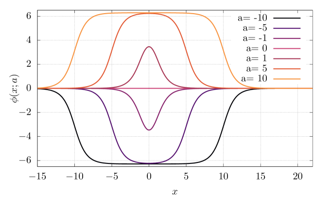
Figure 1: Examples of the naive superposition of the sG kink and antikink (19).

The naive superposition of a kink centred at $-a$ and an antikink centred at $a$ is

$$\phi(x;a)=4\arctan(e^{x+a})-4\arctan(e^{x-a})\,.$$ (18)

Applying the tangent subtraction formula to $\frac{1}{4}\phi$, this becomes

$$\phi(x;a)=4\arctan\left(\frac{\sinh(a)}{\cosh(x)}\right)\,,$$ (19)

where $a$ takes any real value. This is our moduli space of kink-antikink sG field configurations. For $a\gg 0$ there is a kink on the left and antikink on the right, and $\phi$ is positive; for $a\ll 0$ the kink and antikink are exchanged and $\phi$ is negative. When $a=0$, the configuration is the vacuum $\phi=0$. Configurations for various values of $a$ are shown in Fig. 1.

To model kink-antikink dynamics (both scattering and periodic solutions, i.e., breathers) we treat $a(t)$ as a time-dependent modulus, substitute (19) into the field theory Lagrangian (14) and integrate, thereby obtaining a reduced Lagrangian on moduli space of the general form

$$L_{\rm red}=\frac{1}{2}g(a)\,\dot{a}^{2}-V(a)\,.$$ (20)

The kinetic term of the field theory gives the moduli space metric

$$g(a)=16\left(1+\frac{2a}{\sinh(2a)}\right)$$ (21)

and the remaining terms give the moduli space potential

$$V(a)=16\left[1-\frac{1}{2\cosh^{2}(a)}\left(1+\frac{2a}{\sinh(2a)}\right)\right]\,.$$ (22)

Note that the metric and potential satisfy

$$\frac{1}{2\cosh^{2}(a)}\,g(a)+V(a)=16\,,$$ (23)

a relation that we will explain below. For large $a$, $g(a)\sim 16$ and $V(a)\sim 16-32e^{-2a}$, from which one can derive the well-known static force between an sG kink and antikink at large separation $2a$.

The time-dependence of the modulus $a$ can be found starting from the first integral of the equation of motion derived from (20),

$$\frac{1}{2}g(a)\,\dot{a}^{2}+V(a)=E\,,$$ (24)

and then integrating once more. Both $V$ and the conserved energy $E$ include the rest masses of the kink and antikink, so the critical energy separating scattering solutions from breathers is $E=16$. The motion on moduli space is implicitly given by

$$\pm(t-t_{0})=\int\sqrt{\frac{g(a)}{2(E-V(a))}}\,da\,,$$ (25)

and can be calculated numerically.

Before presenting the solutions, let us recall the analogous exact solutions of sine-Gordon theory. The breather solution

$$\phi(x,t)=-4\arctan\left(\frac{\sqrt{1-\omega^{2}}\sin(\omega t)}{\omega\cosh(\sqrt{1-\omega^{2}}\,x)}\right)$$ (26)

has frequency $\omega$ in the range $(0,1)$ and energy

$$E=16\sqrt{1-\omega^{2}}\,.$$ (27)

This solution exactly matches (19) if we ignore the shape-changing factor $\sqrt{1-\omega^{2}}$ in $\cosh(\sqrt{1-\omega^{2}}\,x)$ and say that the breather has modulus dynamics given by

$$\sinh(a(t))=-\frac{\sqrt{1-\omega^{2}}\sin(\omega t)}{\omega}\,.$$ (28)

The kink-antikink scattering solution is the analytic continuation of the breather, when the frequency becomes imaginary. Setting $\omega=iq$ in (26), with $q$ real, we obtain the solution

$$\phi(x,t)=-4\arctan\left(\frac{\sqrt{1+q^{2}}\sinh(qt)}{q\cosh(\sqrt{1+q^{2}}\,x)}\right)\,.$$ (29)

The reparametrisation $v=q/\sqrt{1+q^{2}}$ leads to the more standard form of the scattering solution

$$\phi(x,t)=-4\arctan\left(\frac{\sinh(\gamma vt)}{v\cosh(\gamma x)}\right)\,,$$ (30)

where $\gamma=1/\sqrt{1-v^{2}}$ is the usual Lorentz factor and $\gamma v=q$. This describes a kink and antikink that approach each other with velocities $v$ and $-v$, having total energy $E=16\gamma=16\sqrt{1+q^{2}}$. By ignoring the Lorentz contraction factor $\gamma$ in $\cosh(\gamma x)$, we identify the exact scattering solution as having modulus dynamics

$$\sinh(a(t))=-\frac{\sinh(\gamma vt)}{v}\,.$$ (31)

The asymptotic form of the solution, for large negative $t$ and $x$, is the incoming kink

$$\phi(x,t)\sim 4\arctan(e^{\gamma(x-vt)-\log v})\,,$$ (32)

and the outgoing kink (with field value shifted down by $2\pi$) has the opposite positional shift.

Particularly relevant is the exact sG solution with the critical energy $E=16$,

$$\phi(x,t)=-4\arctan\left(\frac{t}{\cosh(x)}\right)\,,$$ (33)

which can be regarded either as a scattering solution where the initial incoming velocities have decreased to zero, or as a breather of infinite period, where the kink and antikink reach spatial infinity with zero velocity. It evolves precisely through the configurations in our moduli space, with

$$\sinh(a(t))=-t\,.$$ (34)

Equation (34) also solves the equation of motion for $a(t)$ on the moduli space, because a solution of the field equation, being a stationary point of the action for unconstrained field variations, is automatically a stationary point of the action for a smoothly embedded set of constrained fields (the fields in the moduli space), provided the Lagrangian of the constrained problem is the restriction of the Lagrangian of the unconstrained problem, as here. This has an interesting consequence. Differentiating (34), we see that $\cosh(a(t))\,{\dot{a}}=-1$, and substituting this into the energy conservation equation (24) we derive the relation (23) between the metric and potential on moduli space.

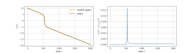
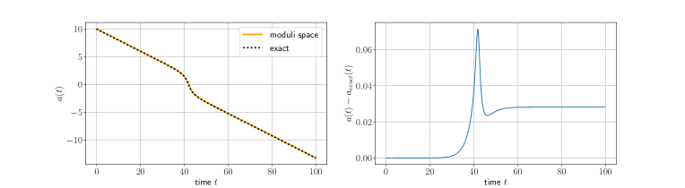
Figure 2: Comparison of the dynamics of the modulus $a$ derived from the moduli space evolution (25), with the exact nonrelativistic solution (35). The small difference is shown magnified on the right. Here the initial kink velocity is $v=0.01$ (upper panels) and $v=0.2$ (lower panels).

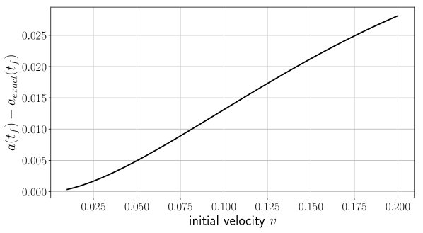
Figure 3: Difference between the asymptotic value of the modulus $a$ derived from the moduli space evolution (25), and from the exact nonrelativistic solution (35), as a function of velocity. Here $t_{f}=100$.

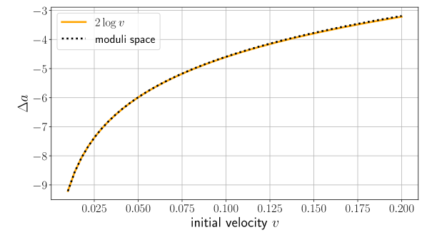
Figure 4: The positional shift $\Delta a$ in a kink-antikink collision derived from the moduli space evolution (25), compared with the exact nonrelativistic result $2\log v$.

Let us now investigate the accuracy of the moduli space dynamics above and below the critical energy $E=16$. If $E>16$ then $a\to\mp\infty$ as $t\to\pm\infty$ and there is kink-antikink scattering. The kink effectively passes through the antikink. In Fig. 2 we compare the moduli space evolution of $a(t)$ according to (25) (solid line) with the nonrelativistic version of the exact evolution (31) (dotted line),

$$\sinh(a(t))=-\frac{\sinh(vt)}{v}\,.$$ (35)

The agreement is very good. There is a very small discrepancy that grows with the velocity, shown in Fig. 3. In Fig. 4 we show the positional shift of $a$ away from a linear evolution in time, due to the collision. The solid line represents the exact, nonrelativistic shift

$$\Delta a=2\log v\,,$$ (36)

while the dotted line is our numerical result from the moduli space dynamics. The agreement is again striking.

If $E<16$ then $a$ oscillates in the moduli space dynamics between turning points $\pm a_{\rm max}$ (where the kinetic energy vanishes) given by

$$V(\pm a_{\rm max})=16\left[1-\frac{1}{2\cosh^{2}(a_{\rm max})}\left(1+\frac{2a_{\rm max}}{\sinh(2a_{\rm max})}\right)\right]=E\,.$$ (37)

This motion corresponds to a breather. Its period, as a function of $a_{\rm max}$, is

$$\sqrt{2}\int_{-a_{\rm max}}^{a_{\rm max}}\sqrt{\frac{g(a)}{V(a_{\rm max})-V(a)}}\,da\,,$$ (38)

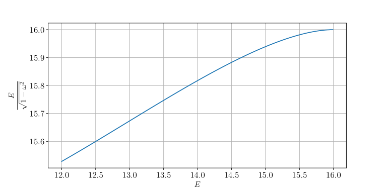
Figure 5: $E/\sqrt{1-\omega^{2}}$ vs. $E$ for the periodic solutions of the moduli space dynamics.

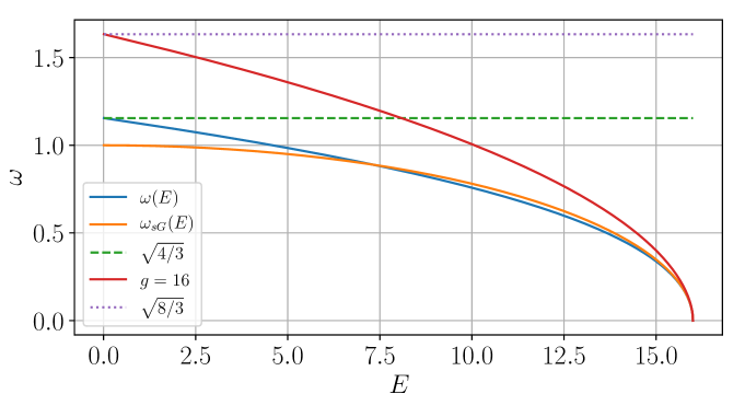
Figure 6: Frequency vs. energy for the sine-Gordon breather, $\omega_{\rm sG}(E)$, and for the periodic solutions of the moduli space dynamics, $\omega(E)$. The upper curve (red) shows the moduli space result if the metric coefficient is fixed at its asymptotic value $g=16$.

and the frequency $\omega$ is $2\pi$ divided by this. In Fig. 5 we plot $E/\sqrt{1-\omega^{2}}$ for the moduli space dynamics, and compare with the ratio $16$ for the exact sG breather. The ratios agree as the energy $E$ approaches $16$ (i.e., as $a_{\rm max}\to\infty$). In Fig. 6 we plot $\omega$ against $E$ for the exact breather and for the oscillating solutions in the moduli space over a larger range. Again the agreement is good, especially as $E\to 16$. The agreement is substantially worse if the variation of the metric $g$ with $a$ is ignored in the moduli space dynamics (i.e., if it is fixed to its asymptotic value $g=16$). This is also shown.

Note that the exact breather’s frequency approaches $1$ as its amplitude goes to zero, whereas in the moduli space dynamics the limiting frequency is $\sqrt{\frac{4}{3}}$. The difference is because the moduli space dynamics uses a field profile of constant width, whereas the exact breather gets arbitrarily broad. The broadening can be interpreted as the analytic continuation of the Lorentz contraction of a colliding kink and antikink, and is ignored in the moduli space approach.

III.2 Kink-antikink-kink dynamics in sine-Gordon theory

The kink-antikink-kink analogue of the naive superposition of a kink and antikink in sine-Gordon theory is

$$\phi(x;b)=4\arctan(e^{x+b})-4\arctan(e^{x})+4\arctan(e^{x-b})\,.$$ (39)

To simplify, we have restricted attention to configurations that are (anti)symmetric in $x$, in the sense that $\phi(-x)=2\pi-\phi(x)$. Using the tangent addition formula

$$\tan(\alpha+\beta+\gamma)=\frac{\tan(\alpha)+\tan(\beta)+\tan(\gamma)-\tan(\alpha)\tan(\beta)\tan(\gamma)}{1-\tan(\alpha)\tan(\beta)-\tan(\alpha)\tan(\gamma)-\tan(\beta)\tan(\gamma)}$$ (40)

we can rexpress (39) as

$$\phi(x;b)=4\arctan\left(\frac{(2\cosh(b)-1)e^{x}+e^{3x}}{1+(2\cosh(b)-1)e^{2x}}\right)\,.$$ (41)

This configuration is symmetric in $b$, and $2\cosh(b)-1$ is nowhere less than $1$. When $b=0$ it becomes a single kink.

For these kink-antikink-kink configurations, the derivative $\frac{\partial\phi}{\partial b}$ vanishes at $b=0$, so the metric coefficient $g(b)$ on the moduli space vanishes there too. The moduli space is incomplete. This problem is resolved by extending to the set of configurations

$$\phi(x;\mu)=4\arctan\left(\frac{\mu e^{x}+e^{3x}}{1+\mu e^{2x}}\right)\,,$$ (42)

where $\mu$ takes any real value greater than $-1$. For large positive $\mu$ we have a chain of kink, antikink and kink, and for $\mu=1$ a single kink. When $\mu=0$ the configuration is a compressed kink $\phi(x)=4\arctan(e^{3x})$, and when $\mu$ is negative the kink is compressed further and acquires bumps outside the usual range of field values $[0,2\pi]$. The bumps extend down to $-\pi$ and up to $3\pi$ as $\mu\to-1$, and the configuration is asymptotically a half-antikink on the left (interpolating between 0 and $-\pi$), a compressed double-kink in the middle (interpolating between $-\pi$ and $3\pi$) and another half-antikink on the right (interpolating between $3\pi$ and $2\pi$). Examples of these configurations are plotted in Fig. 7.

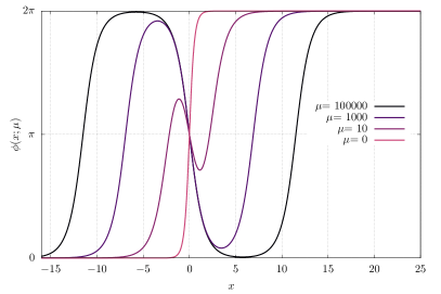
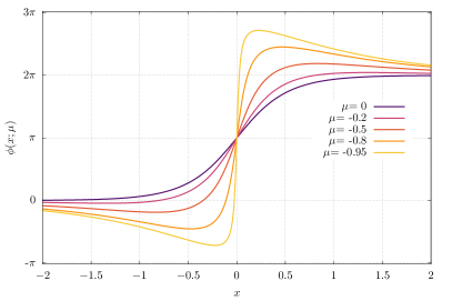
Figure 7: Examples of kink-antikink-kink configurations (42).

The metric on this moduli space, in terms of $\mu$, is

$$g(\mu)=\frac{16}{(\mu-1)(\mu+3)}\left[1-\frac{4}{(\mu+1)\sqrt{(\mu-1)(\mu+3)}}\mbox{arccoth}\left(\frac{1+\mu}{\sqrt{(\mu-1)(\mu+3)}}\right)\right]\,.$$ (43)

It is smooth and positive definite, but becomes singular as $\mu\to-1$. The metric and potential are shown in Fig. 9 (left panel). The dynamics on the moduli space gives a reasonably good description of symmetric kink-antikink-kink motion in sG theory.

However the exact sG kink-antikink-kink solutions involve somewhat different field configurations. There is an analogue of a breather solution in this sector CQS ,

$$\phi(x,t)=4\arctan\left(\frac{(1+\beta)e^{x}+(1-\beta)e^{x+2\beta x}-2\beta e^{\beta x}\cos(\alpha t)}{(1-\beta)+(1+\beta)e^{2\beta x}-2\beta e^{x+\beta x}\cos(\alpha t)}\right)\,,$$ (44)

where the parameters $\alpha$ and $\beta$ must satisfy $\alpha^{2}+\beta^{2}=1$. This solution has frequency $\alpha$ and its amplitude depends on $\beta$. When $\alpha\to 1$ and $\beta\to 0$ it reduces to a static single kink, and for small $\beta$ it is known as a wobbling kink, or wobbler.

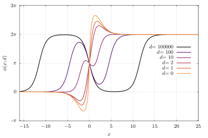
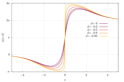
Figure 8: Examples of kink-antikink-kink configurations (46).

We are interested in the opposite limit, where $\alpha\to 0$ and $\beta\to 1$. Taking this limit carefully, one finds the analogue of the critical breather with infinite period, the solution

$$\phi(x,t)=4\arctan\left(\frac{(1+2t^{2}+2x)e^{x}+e^{3x}}{1+(1+2t^{2}-2x)e^{2x}}\right)\,.$$ (45)

This has energy $E=24$, and approaches a configuration with an infinitely separated kink, antikink and kink at rest as $|t|\to\infty$.

Notice that because of the terms $2x$ in formula (45), the field differs at all times from the configurations (42). We therefore define a variant moduli space with configurations

$$\phi(x;d)=4\arctan\left(\frac{(d+2x)e^{x}+e^{3x}}{1+(d-2x)e^{2x}}\right)\,.$$ (46)

The solution (45) moves precisely through this moduli space, but only along the half-line $d\geq 1$. For the same reason as before, we need $d$ to extend through zero to negative real values to have a metrically complete moduli space, and to accommodate dynamics with energy greater than 24. The allowed range is again $d>-1$, because the configuration approaches an infinitely steep double-kink sandwiched between two half-antikinks as $d\to-1$. Bumps occur here for positive and negative values of $d$, see Fig. 8.

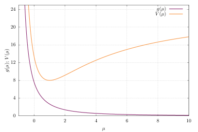
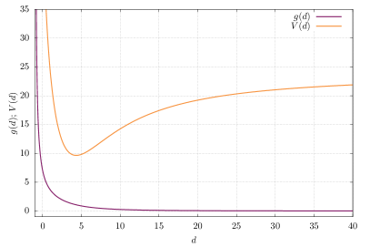
Figure 9: The moduli space metric $g$ and potential $V$ for the kink-antikink-kink configurations (42) (left) and (46) (right).

The metric $g(d)$ and potential $V(d)$ on the variant moduli space can be calculated in the usual way and are plotted in Fig. 9 (right panel). Because the exact solution (45) moves precisely through this moduli space, $g$ and $V$ are related. Combining the energy equation for the moduli space motion at $E=24$,

$$\frac{1}{2}g(d)\,{\dot{d}}^{2}+V(d)=24\,,$$ (47)

with the time-dependence $d(t)=1+2t^{2}$, implying that ${\dot{d}}^{2}=16t^{2}=8(d-1)$, we obtain the relation

$$4g(d)(d-1)+V(d)=24\,.$$ (48)

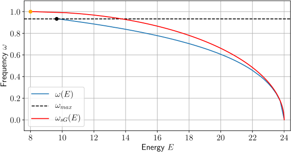
Figure 10: Frequency vs. energy for the sine-Gordon wobbler, $\omega_{\rm sG}(E)$, and for periodic motion on the variant moduli space, $\omega(E)$.

Motion on the variant moduli space with energy $E$ less than 24 gives a good approximation to the wobbler. In Fig. 10 we plot frequency vs. energy, $\omega_{\rm sG}(E)$, for the exact wobbler and for its moduli space approximation $\omega(E)$. The curves agree quite well both for wobblers of small amplitude, and for large wobblers, where the constituent solitons move further apart and the oscillating field stays close to the exact solution (45). Also, having extended the moduli space to negative $d$, we can model a symmetrical collision of two incoming kinks with an antikink, with energy greater than 24. The exact solutions describing collisions can be derived from eq.(44) by allowing $\beta$ to be greater than $1$ and $\alpha$ imaginary, and they are well approximated by the moduli space dynamics.

This completes our discussion of moduli space dynamics for kinks and antikinks in sine-Gordon theory. Having a nontrivial metric and potential on the moduli space improves on the results obtained using Newtonian dynamics and the asymptotic kink-antikink force. We now return to $\phi^{4}$ theory.

IV Kink-Antikink Moduli Spaces in $\phi^{4}$ Theory

In this section we discuss more than one moduli space for kink-antikink configurations in $\phi^{4}$ theory. We clarify their global geometry, and how to choose coordinates. Kink-antikink dynamics has been much studied, see e.g. Sug ; Mosh ; CSW ; KG ; no-force ; PLTC , and only one of our moduli spaces is novel.

IV.1 Naive superposition of kink and antikink

The naive superposition of a kink and antikink is a field configuration of the form

$$\phi(x;a)=\tanh(x+a)-\tanh(x-a)-1\,.$$ (49)

For large or modest positive values of $a$ this represents a kink centred at $-a$ and an antikink at $a$. The field is symmetric in $x$, and the centre of mass is at the origin. The field shift by $-1$ is a little awkward, but essential to satisfy the boundary condition $\phi\to-1$ as $x\to\pm\infty$. Note that $\chi(x)=\tanh(x+a)-\tanh(x-a)$ is a linear field of the type we mentioned earlier, approaching zero at spatial infinity.

The configurations (49), possibly modified to give the kink and antikink some velocity, have often been used before, for example as initial data in numerical simulations of kink-antikink collisions. By calculating the potential energy or the energy-momentum tensor for $a\gg 0$, one can find the force between a well-separated kink and antikink.

The space of configurations $\phi(x;a)$ is a candidate 1-dimensional moduli space for a kink-antikink pair with their centre of mass fixed. The modulus $a$ runs along the real line IR. When $a$ is positive, the kink is on the left and the antikink on the right. When $a=0$, the configuration is exactly the vacuum $\phi=-1$. As $a$ becomes negative, the configuration $\phi(x;a)$ is less familiar, but note that $\tanh(x+a)-\tanh(x-a)$ is antisymmetric in $a$ so as $a$ passes through zero, the kink and antikink in some sense pass through each other. For $a$ large and negative, the field interpolates from $-1$ to $-3$ close to $x=a$ and back to $-1$ near $x=-a$. Configurations for various values of $a$ are shown in Fig. 11 (left panel).

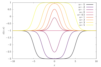
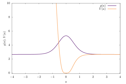
Figure 11: Left: Naive superposition of a $\phi^{4}$ kink and antikink for several values of the modulus $a$. Right: The corresponding moduli space metric and potential.

The potential energy $V(a)$ for field configurations of the form (49) is

$$V(a)=\frac{8}{3}\frac{17+24a+9(-1+8a)e^{4a}-9e^{8a}+e^{12a}}{(-1+e^{4a})^{3}}\,.$$ (50)

It sharply distinguishes positive and negative $a$. For $a\gg 0$ the energy $V$ is approximately $\frac{8}{3}$, twice the kink mass, whereas for $a\ll 0$ it is dominated by the interval of length $2|a|$ where $\phi\approx-3$ and the energy density is approximately $32$; here, $V$ grows linearly with $|a|$. Dynamically there is no reason for $\phi$ to prefer a value close to $-3$, so the field configurations that occur in kink-antikink collisions, even at high speed, are probably never close to configurations with large negative $a$ in this moduli space. $V$ has its minimum at $a=0$, where the configuration is the vacuum.

To find the metric $g(a)$ on the moduli space, we need the derivative with respect to $a$,

$$\frac{\partial\phi}{\partial a}(x;a)=\frac{1}{\cosh^{2}(x+a)}+\frac{1}{\cosh^{2}(x-a)}\,.$$ (51)

This function is non-zero for all $a$, and symmetric in $a$. Integrating its square, following eq.(8), we find

$$g(a)=\frac{8}{\sinh^{2}(2a)}\left(-1+\frac{2a}{\tanh{2a}}\right)+\frac{8}{3}\,.$$ (52)

The metric $g(a)$ and potential $V(a)$ are plotted in Fig. 11 (right panel). Only the metric is symmetric.

It is simple to calculate $g(0)$. $\phi(x;a)$ has the Taylor expansion for $a\approx 0$,

$$\phi(x;a)=-1+\frac{2a}{\cosh^{2}(x)}+O(a^{3})\,.$$ (53)

We call the function $\frac{1}{\cosh^{2}(x)}$ a bump, so the field changes from having a positive bump to a negative bump (around $\phi=-1$) as $a$ changes from positive to negative. At $a=0$, $\frac{\partial\phi}{\partial x}=\frac{2}{\cosh^{2}(x)}$, so

$$g(0)=\int_{-\infty}^{\infty}\frac{4}{\cosh^{4}(x)}\,dx=\frac{16}{3}\,,$$ (54)

eight times the gradient contribution to the kink mass $M$, and therefore equal to $4M$.

In summary, the moduli space of the naive kink-antikink superposition is metrically complete, and motion through this moduli space represents a kink and antikink passing through each other smoothly from positive to negative separation. The reduced Lagrangian on moduli space is

$$L_{\rm red}=\frac{1}{2}g(a)\,{\dot{a}}^{2}-V(a)\,,$$ (55)

and the equation of motion has the first integral

$$\frac{1}{2}g(a)\dot{a}^{2}+V(a)=E\,.$$ (56)

In a kink-antikink collision, $a$ decreases from a positive value and passes through zero, then stops at a maximal negative value determined by energy conservation, and returns to a positive value. While $a$ is negative the field has a negative bump. The time taken for this bounce process can be estimated by solving the equation of motion for $a$. However, numerical exploration of the field equation for $\phi$ shows that this moduli space is too simple to capture important features of kink-antikink dynamics. Most importantly, there is transfer of energy from the positional motions of the kink and antikink into shape mode oscillations. This can lead to multiple oscillations of $a$ before the kink and antikink emerge, or to kink-antikink annihilation. The next moduli space therefore includes the shape mode.

IV.2 Including the shape mode

A single kink, with profile $\phi(x)=\tanh(x)$, has a small-amplitude shape mode of oscillation

$$\phi(x,t)=\tanh(x)+A(t)\frac{\sinh(x)}{\cosh^{2}(x)}\,,$$ (57)

where $A(t)$ oscillates harmonically with frequency ${\sqrt{3}}$. This discrete frequency is below the frequencies of continuum radiation modes which start immediately above 2. Large amplitude oscillations of $A$ are not exact solutions of the field equation. Energy is converted into radiation through a nonlinear process, and $A$ slowly decays.

Configurations of a single kink, including this mode, are

$$\phi(x;a,A)=\tanh(x-a)+A\frac{\sinh(x-a)}{\cosh^{2}(x-a)}\,.$$ (58)

The moduli space is 2-dimensional, with coordinates $a$ and $A$ both taking values in all of IR. As the derivatives of $\phi$ with respect to $a$ and $A$ are both non-zero functions, and linearly independent, the metric is positive definite. Its explicit form is

$$g_{aa}=\frac{4}{3}+\frac{\pi}{2}A+\frac{14}{15}A^{2}\,,\quad g_{aA}=0\,,\quad g_{AA}=\frac{2}{3}\,.$$ (59)

Thus $a$ and $A$ are globally good coordinates. The moduli space dynamics describes a kink that oscillates indefinitely while also moving at a steady mean velocity.

A set of field configurations for a kink at $-a$ and an antikink $a$ that includes this mode for each of them is

$$\phi(x;a,A)=\tanh(x+a)-\tanh(x-a)+A\left(\frac{\sinh(x+a)}{\cosh^{2}(x+a)}-\frac{\sinh(x-a)}{\cosh^{2}(x-a)}\right)-1\,.$$ (60)

Again, the moduli space is 2-dimensional with coordinates $a$ and $A$. The centre of mass is fixed at the origin, and the amplitudes of the shape modes are correlated so that $\phi$ is symmetric in $x$. This restricted set of fields is adequate for initial kink-antikink data having the symmetry. The more general set of field configurations where the shape mode amplitudes are independent was introduced by Sugiyama Sug and has been investigated by Takyi and Weigel TW and others.

For a well-separated kink-antikink pair, it is clear that $a$ and $A$ are good coordinates. $a$ can be positive or negative, and the shape mode usefully allows a change of shape of both kink and antikink. However, at $a=0$ there is a problem, because the shape modes cancel out and $A$ fails to be a good coordinate. The derivatives of $\phi$ with respect to $a$ and $A$ need to be non-zero and linearly independent functions for the metric on moduli space to be positive definite (in these coordinates). This requirement is not satisfied at $a=0$ because the derivative with respect to $A$ is zero. This problem was noted by Takyi and Weigel as a null-vector problem.

The problem has a simple resolution by a change of coordinates. Replace $A$ by $\frac{B}{f(a)}$ where $f(a)$ is any antisymmetric function of $a$ that is linear for small $a$. The linear behaviour near $a=0$ is important to remove the apparent metric singularity, and allow for a smooth field evolution through $a=0$, but otherwise the choice of $f$ is arbitrary. A change of $f$ corresponds to a change in the coordinate $B$, but the moduli space geometry is invariant. One could choose $f(a)=a$ but we prefer $f(a)=\tanh(a)$, as $B$ is then the amplitude of the shape mode, up to a sign, for large $|a|$. The moduli space of field configurations is now

$$\phi(x;a,B)=\tanh(x+a)-\tanh(x-a)+\frac{B}{\tanh(a)}\left(\frac{\sinh(x+a)}{\cosh^{2}(x+a)}-\frac{\sinh(x-a)}{\cosh^{2}(x-a)}\right)-1\,,$$ (61)

and the function of which $B$ is the coefficient has a smooth, non-zero limit as $a\to 0$. Using the Taylor expansion or equivalently l’Hôpital’s rule, one finds for small $a$ the leading terms

$$\phi(x;a,B)\approx 2a\frac{1}{\cosh^{2}(x)}+2B\left(\frac{2}{\cosh^{3}(x)}-\frac{1}{\cosh(x)}\right)-1\,.$$ (62)

As $a$ and $B$ are coefficients of distinct non-zero functions, the moduli space is non-singular in these coordinates and has a smooth metric. More generally, $a$ and $B$ are globally good coordinates, taking values in all of IR.

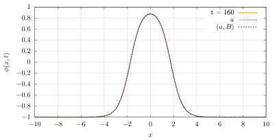
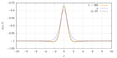
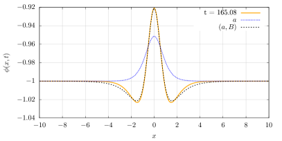
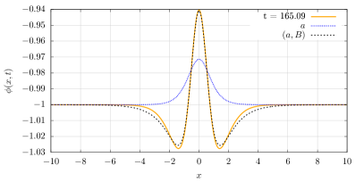
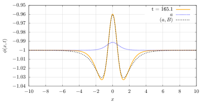
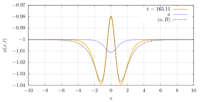
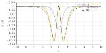
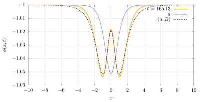
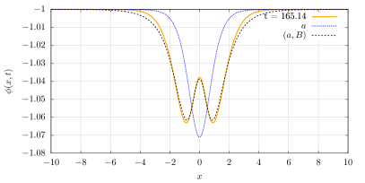
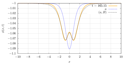
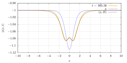
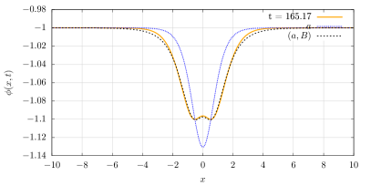
Figure 12: Dynamical kink-antikink field configurations in $\phi^{4}$ theory (solid orange), with best fits to the 1-dimensional ($a$, fine dotted blue) and 2-dimensional moduli space configurations ($(a,B)$, coarse dotted black).

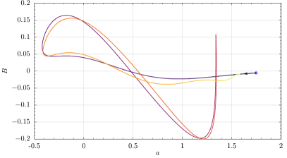
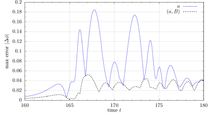
Figure 13: Kink-antikink scattering in $\phi^{4}$ theory. Left: Phase plot for the fitted moduli $(a,B)$. The arrow indicates the initial point and colours denote passing time. Right: Maximal field difference $|\Delta\phi|$ between the true dynamical field $\phi(x,t)$ and the closest moduli space configuration.

The metric on the Sugiyama moduli space has been calculated by Pereira et al. PLTC , using contour integration to evaluate the integrals. It should not be difficult to recalculate the metric on the 2-dimensional subspace of configurations (61), using the coordinates $a$ and $B$. The spatial integrals defining the metric coefficients are not affected, but need to be combined differently. Including distinct amplitudes for the two shape modes adds no further difficulties, because there is no additional null-vector when the shape modes centred at $-a$ and $a$ are added rather than subtracted.

We have found that kink-antikink dynamics in $\phi^{4}$ field theory follows a trajectory through this 2-dimensional moduli space quite well. We have evolved a kink and antikink starting nearly at rest at a large separation, with initial velocity $v=0.05$, and have matched the field configuration at each time $t$ to the configuration in the moduli space with the smallest maximal difference in field value $\phi$, thereby determining a trajectory $(a(t),B(t))$ in moduli space. The true dynamical configuration and the moduli space configuration are shown in Fig. 12 at various times close to the first collision. Also shown is the closest configuration in the naive moduli space with the single modulus $a$ – the fit is clearly less good. The $(a,B)$ trajectory is plotted in Fig. 13, left panel, for $0\leq t\leq 200$. It is smooth even though $a$ passes through zero a couple of times, because of the use of the new coordinate $B$. The maximal field difference is shown in Fig. 13, right panel. It is very small for all $t$ provided the 2-dimensional moduli space is used. What remains to be investigated is whether this trajectory is approximately reproduced by the moduli space dynamics for $a$ and $B$. Calculating the metric and potential on the 2-dimensional moduli space (and also their derivatives) and solving for the dynamics is challenging and will be reported elsewhere.

IV.3 Weighted kink-antikink configurations

Here we discuss a variant of the naive kink-antikink superposition, where the kink and antikink profiles are given a weight that depends on their separation. The weight allows for the kink to be modified by the nearby presence of the antikink, and vice versa. The field configurations now have the form

$$\phi(x;a)=\tanh(a)(\tanh(x+a)-\tanh(x-a))-1\,.$$ (63)

We do not include the shape modes here, although their inclusion would be straightforward. The choice of weight function $\tanh(a)$ is motivated by the identity

$$\tanh(a)(\tanh(x+a)-\tanh(x-a))-1=\frac{c-\cosh^{2}(x)}{c+\cosh^{2}(x)}\,,$$ (64)

where $c=\sinh^{2}(a)$; conveniently, the expression on the right hand side occurs in the iterated kink scheme MOW that we review in the next section. The identity is verified by writing

$$\tanh(x+a)-\tanh(x-a)=\frac{\sinh(x+a)\cosh(x-a)-\cosh(x+a)\sinh(x-a)}{\cosh(x+a)\cosh(x-a)}\,,$$ (65)

and then using hyperbolic analogues of trigonometrical addition and double angle formulae.

For large positive $a$, the weighted superposition agrees with the naive superposition. Curiously, it also agrees for small positive $a$, because to leading order the weighted superposition is $\phi=\frac{2a^{2}}{\cosh^{2}(x)}-1$ whereas the naive superposition is $\phi=\frac{2a}{\cosh^{2}(x)}-1$. The field configurations have the same form, with a positive bump, but the parameter $a$ has changed its meaning. For intermediate $a$, the configurations are slightly different, no matter how the parameters are matched.

However, the moduli spaces of naive and weighted superpositions are metrically quite different as $a$ approaches zero, and if one attempts to extend beyond here. Recall that the naive superposition can be extended smoothly to negative $a$, and the positive bump becomes a negative bump. On the other hand, the weighted superposition (63) is symmetric in $a$, so its moduli space is completely covered by $a$ in the range $0\leq a<\infty$. This moduli space has a boundary at $a=0$ and is geodesically incomplete, because $\phi$ depends quadratically on $a$ for small $a$, so

$$\frac{\partial\phi}{\partial a}=O(a)$$ (66)

and the metric coefficient is $g(a)=O(a^{2})$. $a$ is not a good coordinate near $a=0$ for the weighted superposition, but $c=\sinh^{2}(a)$ is a better coordinate, as $c\approx a^{2}$ for small $a$, and in terms of $c$ the metric coefficient is $g(c)=O(1)$. This can be verified directly using the expression on the right hand side of (64). A motion in which $a$ evolves smoothly from positive through zero to negative is not acceptable dynamically. (It is like the motion of a particle along a line that stops and reverses, even though no force acts.) Instead, a motion where $c$ evolves smoothly through zero is acceptable.

The natural range of $c$ is the interval $(-1,\infty)$, as $\phi$ has a singularity at $x=0$ when $c=-1$. When $c<0$, the field configuration has a negative bump with a different shape from the bump that occurs for negative $a$ in the naive kink-antikink superposition. The identity (64) is still valid for $c<0$ if suitably interpreted. $a$ becomes imaginary, so let us write $a=i{\tilde{a}}$ with ${\tilde{a}}$ positive. (We will comment further on the signs of $a$ and ${\tilde{a}}$ below.) Recall the relations

$$\sinh(i{\tilde{a}})=i\sin({\tilde{a}})\,, \sin(i{\tilde{a}})=i\sinh({\tilde{a}})\,,$$

$$\cosh(i{\tilde{a}})=\cos({\tilde{a}})\,, \cos(i{\tilde{a}})=\cosh({\tilde{a}})\,.$$ (67)

Therefore, $c=-\sin^{2}({\tilde{a}})$ for negative $c$, and we can express the weighted superposition of kink and antikink (63) as

$$\phi(x;{\tilde{a}})=i\tan({\tilde{a}})(\tanh(x+i{\tilde{a}})-\tanh(x-i{\tilde{a}}))-1\,.$$ (68)

This expression is real, and symmetric in ${\tilde{a}}$. Use of the subtraction formula for the $\tanh$ function leads back to the formula for $\phi$ in terms of $c$.

The interpretation of (68) is that the kink and antikink have imaginary positions $\pm i{\tilde{a}}$. The moduli space is well defined in terms of $c$ and motion through $c=0$ is unproblematic, but it corresponds to a 90-degree scattering of the positions of the kink and antikink. Such scattering is familiar in the dynamics of solitons in higher dimensions, for example for vortices and monopoles, where the scattering occurs in a real 2-dimensional plane. Here, remarkably, the scattering occurs in the complex plane of the 1-dimensional kink position parameter $a$. This type of scattering is only possible because the sign of $a$ is not fixed. The kink and antikink are initially located on the real axis at $-a$ and $a$, but because of the weight factor, there is no effect if $a$ is replaced by $-a$. The kink and antikink later appear on the imaginary axis at ${\tilde{a}}$ and $-{\tilde{a}}$, and note that because the amplitude $i\tan({\tilde{a}})$ is imaginary, the kink and antikink cannot now be distinguished. Therefore the scattering does not break the reflection symmetries of the complexified $a$-plane. A pair of points scatters from the real to the imaginary axis, in the same way that the algebraic roots of $z^{2}=c$ scatter as $c$ passes through zero along the real axis.

The moduli space with coordinate $c$ is geodesically complete, for $c$ extending to $-1$. This could be verified by calculating the metric factor $g(c)$, but is easier to see as follows. The limiting (singular) field configuration is

$$\phi(x;c=-1)=-1-\frac{2}{\sinh^{2}(x)}\,,$$ (69)

whereas $\phi(x;c=0)=-1$. In the field configuration space, the squared distance (5) between these configurations is the integral of $\frac{4}{\sinh^{4}(x)}$, but this is divergent. The distance in the moduli space between $c=0$ and $c=-1$ (which is not a straight path in field configuration space, so not shorter) is therefore also infinite.

In summary, the moduli space of a superposed weighted kink and antikink is an interesting alternative to the more familiar moduli space of the naive superposition. For this new moduli space to be geodesically complete, one must allow for the kink and antikink to scatter in the complexified plane of their positions $a$ and $-a$. However the field remains real, and in terms of the modulus $c$ the field just transitions from having a positive bump to a negative bump as $c$ passes through zero. Further investigation is needed to see if this moduli space is better than the moduli space of the naive superposition for modelling kink-antikink dynamics in the full field theory. It is almost certainly necessary to include shape modes in either case.

V Iterated Kinks

In this section we briefly review the iterated kink equation that was introduced by three of the present authors in MOW . It is a sequence of ODEs,

$$\frac{d\phi_{n}}{dx}=-(1-\phi_{n}^{2})\phi_{n-1}\,,\quad n=1,2,3,\dots\,,$$ (70)

where we fix $\phi_{0}(x)=-1$. For all $n$ we impose the boundary condition $\phi_{n}(x)\to-1$ as $x\to-\infty$. The equations are solved sequentially, and one can stop at any $n$. We will only discuss the solutions in any detail up to $n=3$. For odd (even) $n$, the generic solution $\phi_{n}$ approaches $+1$ ($-1$) as $x\to\infty$. For odd $n$, we therefore impose the boundary condition $\phi_{n}(x)\to+1$ as $x\to\infty$; then the solution always lies between $-1$ and $+1$. For even $n$, the solutions are essentially of two types: a solution either lies between $-1$ and $+1$, or is everywhere less than $-1$. These types are separated by the constant solution $\phi_{n}(x)=-1$. As each equation of the iterated kink sequence is of first order, its solution has one constant of integration. If we retain all of these, the $n$th iterate $\phi_{n}$ depends on $n$ arbitrary constants – the moduli of the $n$th iterate. For even $n$, the constant solution $\phi_{n}(x)=-1$ lies in the interior of the moduli space.

The iterated kink equation is a systematic extension of the idea of a kink equation with impurity $\chi(x)$ BPS-imp ; BPS-susy ; Solv

$$\frac{d\phi}{dx}=-(1-\phi^{2})\chi(x)\,,$$ (71)

which in turn is a generalisation of the basic first order ODE for a $\phi^{4}$ kink or antikink, $\frac{d\phi}{dx}=\pm(1-\phi^{2})$.

The iterated kink solutions are interesting because a large part of the moduli space of the $n$th iterate consists of field configurations with $n$ alternating kinks and antikinks at arbitrary separations (starting with a kink on the left). Other parts of the moduli space consist of configurations where a kink-antikink pair, or more than one pair, have approached each other to form a bump. The moduli space of the $n$th iterate therefore usefully describes configurations of $n$ kinks and antikinks. However these configurations do not incorporate the standard shape mode deformations of a kink or antikink.

We conjecture that each of these moduli spaces has a positive definite metric and is metrically smooth and geodesically complete, almost everywhere. We have not proved this, but it is clearly true for $n=1$ and $n=2$, and the numerical study for $n=3$ and $n=4$ reported in MOW indicates that the partial derivatives of the field $\phi_{n}(x)$ with respect to all moduli are almost everywhere non-zero and linearly independent. The exceptional points in moduli space are the constant configurations $\phi_{n}(x)=-1$, for even $n$, where a rigid translation has no effect. We will focus on the relative motion of kinks, so this problem with translations does not occur.

Let us now recall the first few iterates. For $n=1$, we have the standard $\phi^{4}$ kink equation, with solution $\phi_{1}(x;a)=\tanh(x-a)$. The moduli space is the real line with its Euclidean metric. For $n=2$, the field $\phi_{1}$ acts as an impurity. As $a$ shifts, the solution $\phi_{2}$ simply shifts with it. Let us therefore ignore this translational modulus, and assume that $\phi_{1}(x)=\tanh(x)$. Then one expression for the solutions $\phi_{2}$ is

$$\phi_{2}(x;c)=\frac{c-\cosh^{2}(x)}{c+\cosh^{2}(x)}\,.$$ (72)

These configurations, which appeared in Section 4, are non-singular for $-1<c<\infty$, and are illustrated in ref.MOW . Note that for $c>0$, $\phi_{2}$ is between $-1$ and $+1$; for $c=0$, $\phi_{2}(x)=-1$; and for $-1<c<0$, $\phi_{2}$ is everywhere less than $-1$. The moduli space has no metric singularity at $c=0$.

The third iterate $\phi_{3}(x)$ is obtained from the second iterate $\phi_{2}$ by integrating the relevant ODE. We will only consider the solutions that are antisymmetric in $x$, although the general solution with broken reflection symmetry is known and illustrated in MOW . The only modulus is then $c$, arising from $\phi_{2}$. The antisymmetric solutions $\phi_{3}(x;c)$ are kink-antikink-kink configurations when $c$ is large, having an antikink at the origin and kinks at equal separation on either side. As $c$ approaches zero and becomes negative, the kinks approach and annihilate the antikink, leaving a single kink modified by a variant of the shape mode. In the next section we look at the moduli space of these configurations in more detail.

VI Kink-Antikink-Kink Moduli Spaces in $\phi^{4}$ Theory

Here we investigate three candidate moduli spaces for kink-antikink-kink configurations in $\phi^{4}$ theory, antisymmetric in $x$. Each moduli space is 1-dimensional.

VI.1 Naive superposition of kink, antikink and kink

An obvious choice for a kink-antikink-kink configuration is the generalisation of the naive kink-antikink superposition,

$$\phi(x;b)=\tanh(x+b)-\tanh(x)+\tanh(x-b)\,.$$ (73)

The modulus $b$ parametrises the positions of the two kinks, and the antikink is at the origin. $\phi(x;b)$ is symmetric in $b$. For positive $b$ we have an equally spaced chain of kink, antikink and kink. The kinks approach the antikink as $b\to 0$, and at $b=0$ merge to form the standard single kink at the origin. For negative $b$ this process reverses, so the moduli space is really just the half-line with $b$ non-negative.

The metric on the moduli space depends on the derivative with respect to $b$,

$$\frac{\partial\phi}{\partial b}(x;b)=\left(\frac{1}{\cosh^{2}(x+b)}-\frac{1}{\cosh^{2}(x-b)}\right)\,.$$ (74)

This is antisymmetric in $b$ and vanishes at $b=0$. The resulting metric is

$$g(b)=\frac{2}{3}\,\frac{-24b\cosh(2b)+9\sinh(2b)+\sinh(6b)}{\sinh^{3}(2b)}\,,$$ (75)

and also vanishes at $b=0$. The metric on the half-line is therefore not complete and $b$ is not globally a good coordinate. However, this problem is resolved by extending the moduli space.

Usefully, the field superposition (73) is (minus) the product of the iterated configuration $\phi_{2}$, given by (72), and a kink at the origin $\phi_{1}(x;0)=\tanh(x)$,

$$\phi(x;b)=-\left(\frac{\sinh^{2}(b)-\cosh^{2}(x)}{\sinh^{2}(b)+\cosh^{2}(x)}\right)\tanh(x)=-\phi_{2}(x;c)\phi_{1}(x;0)\,,$$ (76)

where $c=\sinh^{2}(b)$ and is therefore non-negative for real $b$. $c$ is a better choice for the modulus, as we can straightforwardly extend the moduli space to negative values of $c$, although this requires $b$ to be extended to imaginary values $b=i\tilde{b}$, with $\tilde{b}$ positive. Then $c=-\sin^{2}(\tilde{b})$, so the range of $\tilde{b}$ is $0\leq\tilde{b}<\frac{1}{2}\pi$. The new field configurations are more compressed than the standard kink at the origin. $\phi(x;{\tilde{b}})$ becomes not only steeper as $\tilde{b}$ grows, but also acquires negative and positive bumps outside the range of field values $[-1,1]$ as $\tilde{b}$ approaches $\frac{1}{2}\pi$. These bumps are produced by the large negative bump in $\phi_{2}$ for $c$ approaching $-1$.

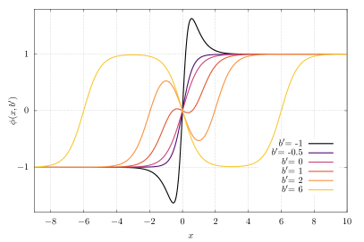
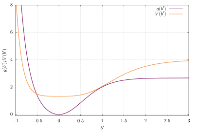
Figure 14: Naive superposition of kink, antikink and kink. Left: Profiles for several values of the extended modulus $b^{\prime}$. Right: The moduli space metric and potential.

At $c=-1$ the potential energy is infinite, so in a dynamical kink-antikink-kink motion $c$ decreases, stops before it reaches $-1$, and increases again. In the complex plane of the modulus $b$, there is 90-degree scattering during a kink-antikink-kink collision, which occurs in reverse as the motion reverses. From the perspective of the naive superposition, the kinks scatter but the antikink remains at rest at the origin. In Fig. 14 we plot the field configurations as well as the metric and potential on moduli space as a function of $b$. We show these for the real and imaginary ranges of $b$ simultaneously by introducing a new real coordinate $b^{\prime}$ defined by

$$b^{\prime}=\left\{\begin{array}[]{cl}b&\text{for}\;\;b\in[0,\infty)\\ -\tilde{b}&\text{for}\;\;\tilde{b}\in\left[0,\frac{1}{2}\pi\right)\,.\end{array}\right.$$ (77)

Note that, under the replacement $b\to i\tilde{b}$, the metric (75) acquires an additional minus sign to compensate $\dot{b}^{2}$ being negative in the kinetic part of the Lagrangian. There is not a genuine sign problem, and the metric is positive if $c$ is used as the coordinate.

VI.2 Iterated kink-antikink-kink

The iterated kink scheme gives an alternative moduli space of kink-antikink-kink configurations. Iterating the $\phi_{2}$ solution, with its modulus $c$, we obtain the $\phi_{3}$ solution

$$\phi_{3}(x;c)=\tanh\left(x-2\sqrt{\frac{c}{1+c}}\mbox{ arctanh}\left(\sqrt{\frac{c}{1+c}}\tanh(x)\right)\right)\,.$$ (78)

There is no further modulus derived from the constant of integration because we select antisymmetric configurations with equal kink-antikink-kink spacings. The formula (78) is valid for all $c>-1$, even though the square root is imaginary if $c<0$. $\phi_{3}$ is the standard kink for $c=0$, and is a compressed kink for negative $c$, becoming infinitely steep as $c\to-1$. So $\phi_{3}$ is qualitatively similar to the naive superposition with $b$ continued to imaginary values, but here the field value is always confined to $[-1,1]$, and does not have bumps. These field configurations are shown in Fig. 15.

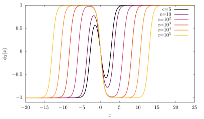
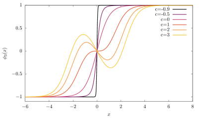
Figure 15: Iterated $\phi_{3}$ solution for several values of the modulus $c$.

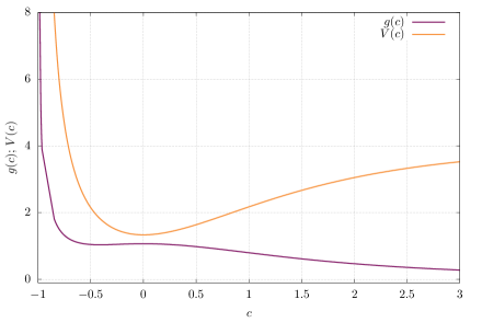
Figure 16: Moduli space metric $g(c)$ and the potential $V(c)$ for the iterated $\phi_{3}$ solutions.

The metric $g(c)$ on this moduli space, together with the potential $V(c)$, are shown in Fig. 16. $g(c)$ is positive so $c$ is a good coordinate. In particular,

$$\frac{\partial\phi_{3}}{\partial c}(x;c=0)=-2\frac{\sinh(x)}{\cosh^{3}(x)}\,,$$ (79)

which gives $g(0)=\frac{16}{15}$. The moduli space is still incomplete, with boundary at $c=-1$, but this does not matter as $V$ is infinite here. For example, the squared distance (5) between the standard kink $\phi_{3}(x;c=0)$ and the boundary configuration $\phi_{3}(x;c\to-1)$ is $s^{2}=2(-1+\ln 4)$.

VI.3 Weighted superposition of kink-antikink-kink

Recall that the kink-antikink configuration $\phi_{2}$ can be expressed exactly as a weighted superposition of kink and antikink, so it could be interesting to find a moduli space of weighted kink-antikink-kink configurations. A general formula introducing a weight $\Lambda(b)$ is

$$\phi(x;b)=\Lambda(b)\tanh(x+b)+(1-2\Lambda(b))\tanh(x)+\Lambda(b)\tanh(x-b)\,.$$ (80)

This configuration is antisymmetic in $x$ and satisfies the vacuum boundary conditions. The naive superposition has $\Lambda=1$, but allowing non-constant $\Lambda$ could be an improvement.

The weighted superposition is quite close to the iterated kink solution $\phi_{3}(x;c)$ for a suitable choice of $b$ and $\Lambda(b)$ in terms of $c$. For $c$ negative, $b$ becomes imaginary and we again introduce the extended modulus $b^{\prime}$. In Fig. 17 we plot the optimal $b$ and $\Lambda(b)$, found using a least squares fit of $\phi(x;b)$ to $\phi_{3}(x;c)$. For large $c$, the kinks are well-separated from the antikink, so $\Lambda\approx 1$ and $b\approx\log(4c)$. When $c$ is close to zero, the best fit is with $b\approx\sqrt{\frac{7c}{3}}$ and $\Lambda=\frac{3}{7}$. Strictly speaking, $\Lambda$ is indeterminate when $c=0$, but these values of $b$ and $\Lambda$ give the best fit nearby, giving an exact fit up to quadratic order in $c$ in the Taylor expansion of $\phi_{3}(x;c)$. $\Lambda$ decreases towards zero as $c$ approaches $-1$. Here $\phi_{3}$ approaches a step function, and the fit is not very good.

These weighted kink-antikink-kink superpositions with numerically determined coefficients are probably not very useful, especially since they are close to the iterated kink configurations $\phi_{3}$. More interesting could be a moduli space of configurations obtained using a suitable analytic formula for the weight $\Lambda(b)$.

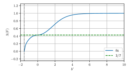
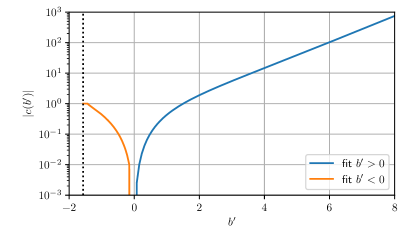
Figure 17: Left: $\Lambda(b^{\prime})$. Right: $c(b^{\prime})$.

VII Conclusions

We have constructed a number of moduli spaces – collective coordinate manifolds – for field configurations of kink and antikink solitons in both $\phi^{4}$ theory and sine-Gordon (sG) theory. These are smooth, finite-dimensional submanifolds of the infinite-dimensional field configuration spaces. Only in parts of the moduli space do the moduli correspond to the real positions of the kinks and antikinks as separated particles. The moduli have a different interpretation when a kink and antikink annihilate and produce a bump in the field, or when a kink-antikink-kink configuration turns into a compressed single kink. For the $\phi^{4}$ kinks we have incorporated an amplitude for the shape mode oscillation (the discrete, normalisable kink oscillation mode whose frequency is below the continuum). For kink-antikink and also kink-antikink-kink configurations, we have assumed a spatial reflection symmetry to simplify the analysis.

By restricting the field theory Lagrangian to field configurations evolving through moduli space, we obtain, through spatial integration, a reduced Lagrangian with kinetic and potential terms on moduli space, whose equation of motion is an ODE. The coefficient matrix of the kinetic term is interpreted as a Riemannian metric on moduli space. (In several of our examples there is just one modulus and the metric is a single function.) A guiding principle is that this metric should be either metrically complete, so that free geodesic motion does not reach any boundary in finite time, or metrically incomplete but with a potential that is infinite at the boundary, so that no dynamical trajectory reaches it.

For a single kink in $\phi^{4}$ or sG theory, there is a 1-dimensional moduli space, with modulus the kink position (centre) $a$. The metric is Euclidean and the potential constant, so kink motion is at constant velocity. Shape mode oscillations of the $\phi^{4}$ kink can also be accommodated. Moduli space dynamics is a fundamentally non-relativistic approximation, so the kink is not Lorentz contracted.

The simplest moduli space for kink-antikink dynamics in $\phi^{4}$ theory is obtained using a naive superposition of the kink and antikink, with the centres at $-a$ and $a$ respectively. The modulus $a$ runs from $-\infty$ to $\infty$ and the moduli space is complete. An interesting alternative moduli space uses a weighted kink-antikink superposition. When the weight factor is $\tanh(a)$, the configurations are identical to those occurring in the iterated kink scheme MOW . This observation is useful, because the moduli space in terms of $a$ is now incomplete. The reason is that the weighted configurations are symmetric in $a$, so the moduli space is just the half-line $a\geq 0$, bounded by the vacuum configuration ($a=0$) where the kink and antikink annihilate. On the other hand, the iterated kink configuration has a different modulus $c=\sinh^{2}(a)$ that extends through $0$ down to $-1$. The extended moduli space in terms of $c$ is complete. Motion in this moduli space allows the kink and antikink to approach from large separation, smoothly pass through the vacuum configuration, stop at a configuration with a negative bump, and bounce back. In terms of the original position modulus $a$ – just a change of coordinate – there has been scattering from real to imaginary values and back, although the field remains real. This remarkable 90-degree scattering of the complexified position coordinate $a$ is reminiscent of the real 90-degree scattering that occurs for several types of soliton in two or three spatial dimensions.

We have also reconsidered the well-known moduli space that includes the shape modes of the $\phi^{4}$ kink and antikink (still preserving a reflection symmetry). This was introduced by Sugiyama Sug , and studied by a number of authors, including Takyi and Weigel TW , who clarified details of the metric structure but also reported a null-vector problem – a zero in the metric. We have shown here that this null-vector is an artifact of the coordinate choice, and disappears if the shape mode amplitude $A$ is replaced by $B=A/\tanh(a)$ (the denominator could be any function linear in $a$ near $a=0$).

In the sG case, the moduli space of naive kink-antikink superpositions consists, surprisingly, of the same field configurations that occur in the exact kink-antikink solution at the critical energy $16$ separating kink-antikink scattering solutions from breathers. Using the energy conservation law for the exact solution, we obtain a nice relation between the metric and potential on this moduli space (which provides a useful check on the calculations). The moduli space is complete, and we have shown that the dynamics on it gives a good approximation to the exact scattering and breather solutions with energies above and below $16$. This relies on comparing the frequency vs. energy relations for the exact breathers and for the approximate breathers modelled by moduli space dynamics, and comparing the exact positional shift that occurs in kink-antikink scattering with the moduli space approximation to this.

We have also considered kink-antikink-kink moduli spaces, where the two kinks are equidistant from the antikink at the origin. The moduli space of two naively superposed kinks and an antikink allows the kinks to approach and annihilate the antikink, leaving a single kink. However this moduli space is incomplete, and needs to be extended to allow the single kink to become more compressed (steeper). We have proposed how to do this, both in $\phi^{4}$ and sG theory. The kink position coordinates are imaginary in this extension, although the field again remains real. The resulting moduli spaces are still incomplete, having a boundary configuration that is a step function – an infinitely steep kink that is only a finite distance from a smooth kink. However, the step function has infinite potential energy, so the dynamics on moduli space does not reach the boundary.

In the sG case there is an exact solution having critical energy 24 separating the kink-antikink-kink scattering solutions from the wobbling kink solutions. Its configurations define a useful alternative moduli space, but this moduli space is again incomplete and has to be extended to accommodate dynamics with energy larger than 24. This is another example where the metric and potential are simply related.

We have reported preliminary tests of the 2-dimensional moduli space approximation to (reflection-symmetric) kink-antikink dynamics in $\phi^{4}$ theory, using our improved coordinate for the shape mode amplitude, but more remains to be done. The field equation, a PDE, has been solved numerically, and we have shown that the field evolution is close to a motion through the moduli space. $\phi^{4}$ theory is more complicated than sG theory, because of the shape modes and because of the radiation emitted. Despite much work in this area for more than 40 years KG , various largely technical difficulties have arisen in attempts to match the field dynamics of kinks and antikinks to finite-dimensional moduli space models of the dynamics. In this paper we have clarified the geometry and full extent of various moduli spaces. This should lead to an improved treatment of the dynamics on them, and to a deeper understanding of the interesting and complicated phenomena observed in kink-antikink interactions.

References

- (1) R. Rajaraman, Solitons and Instantons, Amsterdam, Elsevier Science, 1982.
- (2) P. G. Drazin and R. S. Johnson, Solitons: An Introduction, Cambridge University Press, 1989.
- (3) N. Manton and P. Sutcliffe, Topological Solitons, Cambridge University Press, 2004.
- (4) V. I. Arnol’d, Mathematical Methods of Classical Mechanics, New York Berlin, Springer, 1978.
- (5) E. B. Bogomolny, The stability of classical solutions, Sov. J. Nucl. Phys. 24, 449 (1976).
- (6) A. Jaffe and C. Taubes, Vortices and Monopoles, Boston, Birkhäuser, 1980.
- (7) N. S. Manton, The force between ’t Hooft-Polyakov monopoles, Nucl. Phys. B126, 525 (1977).
- (8) N. S. Manton, A remark on the scattering of BPS monopoles, Phys. Lett. B110, 54 (1982).
- (9) M. F. Atiyah and N. J. Hitchin, The Geometry and Dynamics of Magnetic Monopoles, Princeton University Press, 1988.
- (10) T. M. Samols, Vortex scattering, Commun. Math. Phys. 145, 149 (1992).
- (11) T. Sugiyama, Kink-antikink collisions in the two-dimensional model, Prog. Theor. Phys. 61, 1550 (1979).
- (12) M. Moshir, Soliton-antisoliton scattering and capture in theory, Nucl. Phys. B185, 318 (1981).
- (13) D. K. Campbell, J. F. Schonfeld and C. A. Wingate, Resonance structure in kink-antikink interactions in theory, Physica D9, 1 (1983).
- (14) P. G. Kevrekidis, and R. H. Goodman, Four decades of kink interactions in nonlinear Klein-Gordon models: A crucial typo, recent developments and the challenges ahead, https://dsweb.siam.org/The-Magazine/All-Issues/acat/1/archive/102019; [arXiv:1909.03128].
- (15) I. Takyi and H. Weigel, Collective coordinates in one-dimensional soliton model revisited, Phys. Rev. D94, 085008 (2016).
- (16) N. S. Manton, K. Oles and A. Wereszczynski, Iterated kinks, JHEP 1910, 086 (2019).
- (17) E. P. S. Shellard and P. J. Ruback, Vortex scattering in two dimensions, Phys. Lett. B209, 262 (1988).
- (18) M. F. Atiyah and N. S. Manton, Geometry and kinematics of two Skyrmions, Commun. Math. Phys. 153, 391 (1993).
- (19) J. K. Perring and T. H. R. Skyrme, A model unified field equation, Nucl. Phys. 31, 550 (1962).
- (20) S. Cuenda, N. R. Quintero and A. Sánchez, Sine-Gordon wobbles through Bäcklund transformations, Disc. Cont. Dyn. Sys. - S 4, 1047 (2011).
- (21) C. Adam, K. Oles, T. Romanczukiewicz and A. Wereszczynski, Kink-antikink scattering in the model without static intersoliton forces, Phys. Rev. D101, 105021 (2020).
- (22) C. F. S. Pereira, G. Luchini, T. Tassis and C. P. Constantinidis, Some novel considerations about the collective coordinates approximation of the scattering of kinks, arXiv:2004.00571 (2020).
- (23) C. Adam, T. Romanczukiewicz and A. Wereszczynski, The model with the BPS preserving defect, JHEP 1903, 131 (2019).
- (24) C. Adam, J. Queiruga and A. Wereszczynski, BPS soliton-impurity models and supersymmetry, JHEP 1907, 164 (2019).
- (25) C. Adam, K. Oles, J. Queiruga, T. Romanczukiewicz and A. Wereszczynski, Solvable self-dual impurity models, JHEP 1907, 150 (2019).